Download nov18-96 ADAS Bulletin

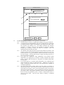
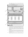
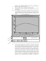
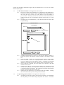
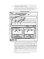
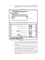
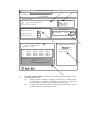
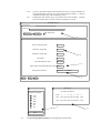
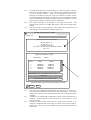
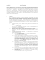
nov18-96
ADAS Bulletin
Five new programs are ready. Two ADAS series 1 data entry and verification programs are operational.
These are ADAS102, for entry and interpolation of electron impact excitation data, and ADAS103 for
entry of dielectronic recombination data. They follow the same broad design principles as other codes
in ADAS series 1. ADAS302, for interrogation of ion/atom collision data, completes the programs
from series 3. Finally ADAS402, for interrogation of iso-nuclear master files, and ADAS404 for
conversion of isoelectronic master files to isonuclear master files completes ADAS series 4. Note that
the old IBM ADAS403 code has been subsumed in ADAS404 for the moment. A more sophisticated
treatment will be released in the future.
1.
ADAS102
This is a program for examination of electron collision rate coefficient data from external
sources and for its interpolation to different temperatures for permanent storage in the ADAS
database. There is no central ADAS data class associated with input to this program, since
new data is entered by hand in the program. However a mechanism is provided for storage and
retrieval of the output from the ADAS102 analysis. The output from a case may be stored in
an archive file. Such files are present only on the user’s own space. Storage is sequential with
an index.
1.1.
1.2.
1.3.
Remember to ensure you have a defaults directory allocated. This should have the
pathway
/..../uid/adas/defaults
where uid is your user identifier. The defaults directory records the parameters you
set the last time you ran each ADAS code.
Move to the directory in which you wish ADAS created output text file (paper.txt is
the default) and graphic files (e.g. graph.ps if a postscript file) to be placed.
Initiate ADAS, move to the series 1 menu and click on the second button to activate
ADAS102.
The archive selection window appears first. It is slightly different in operation than
the usual file selection window.
1.3.1. The recommended root path for user archiving for ADAS102 analysis is
/..../uid/adas/arch102/
which may be edited in the usual manner.
1.3.2. Click the appropriate button at a) for opening an old archive file, starting a
new archive file or ignoring archiving. In the first case, the usual file display
window shows existing archive files from which selection may be made. The
selected file is displayed in the selection window. In the second case, the file
display window is the same, but the selection window is editable for entry of
a new archive file name. Remember to press the return key on the
keyboard to record an entered value.
1.3.3. The capability is given for reworking or re-displaying the results of an earlier
analysis stored in an archive file. At b) click on the Refresh from archive
button. Then give the Archive index number. The selected data will be used
as the default data in the subsequent processing and output windows.
Archiving is strictly sequential. A new analysis is simply appended at the
end of the archive file and the index updated. These is no data replacement
or substitution.
1.3.4. Clicking on the Browse Index button displays the index list for the selected
archive file. The possibility of browsing the index appears in the subsequent
main window also.
1.3.5. Clicking the Done button moves you forward to the next window. Clicking
the Cancel button takes you back to the previous window
ADAS102 INPUT
Data root
/home/summers/adas/arch102/
Edit Path Name
Old Archive
New Archive
No Archive
Refresh from Archive
a)
Archive Index Number
b)
dhb95fe_001.dat
. .
dhb95fe_001.dat
.
Archive File
Browse Index
1.4.
Cancel
Done
The processing options window has the appearance shown below
1.4.1. The button Browse Index at a) again allows display of the archive index list.
1.4.2. As described in the ADAS Manual, four types of collisional rate coefficients
are allowed, namely 1-dipole, 2-non-dipole, 3-spin change and 4-other. Enter
the transition type number at b). For dipole transitions the transition
probability is required. Either the line strength (S), absorption oscillator
strength (f) or Einstein A-value (A) forms are accepted. Click the
appropriate button and enter the value.
1.4.3. At c) details of the upper and lower levels of the transition are entered. The
energies of levels are measured upwards from the lowest level of the ion.
Click on the Select energy form button to indicate which units are being used
for these energies. Note that full statistical weights (including spin parts in
the case of terms) are required.
1.4.4. User input rate coefficients, input temperatures and required output
temperatures are displayed at d) with the currently selected units shown
below. Click the Edit table button to ‘drop down’ the ADAS Table Editor
for data input.
1.4.5. If an archive data set is opened, input temperatures, rate coefficients and
output temperature values are filled from this. Otherwise the fields are
empty. Pressing the Default Temperature values button inserts a default set
of output temperatures.
1.4.6. The ADAS Table Editor window follows the same pattern of operation as
described previously. Note however the fairly wide selection of units in
which data can be entered. This is to ease the problem of unit conversion for
data from the general literature. Click on the buttons for the units with which
you wish to work. The program internally converts to the temperature in
Kelvin and the rate parameter Upsilon. If data is returned from archive it
will be in these forms. Click the Done button if editing is completed
satisfactorily.
ADAS102 PROCESSING OPTIONS
Data file name : /home/summers/adas/arch102/dhb95fe_001.dat
Browse Index
Nuclear Charge:
26.00
Transition Type:
1
Transition Probability: 5.40E+10
a)
Form:
f
S
Lower Level
1
Stat. Wt. :
Index :
9.0
Stat. Wt. :
Level Energy : 0.347841
c)
Select Energy Form :
INDEX
1
2
3
4
5
6
7
8
A
Upper Level
b)
Index :
18.00
Ion Charge:
4
9.0
Level Energy : 8.705277
cm-1
Rydbergs
Input Temp.
Input Coefft.
Output Temp.
1.000E+00
2.000E+00
5.000E+00
1.000E+01
2.000E+01
5.000E+01
1.000E+02
2.000E+02
1.000E+00
2.000E+00
5.000E+00
1.000E+01
2.000E+01
5.000E+01
1.000E+02
2.000E+02
1.000E+05
2.000E+05
3.000E+05
4.000E+05
7.000E+05
8.000E+05
1.000E+06
2.000E+06
Input Temp. units : Reduced. Input Rate Coefft.: Upsilon . Output Temp. units :
Edit Table
d)
Default Temperature values
Edit the processing options data and press Done to proceed
Cancel
1.4.7.
1.5.
Done
Clicking the Done button causes the next output options window to be
displayed. Remember that Cancel takes you back to the previous window.
The Escape to Menu icon is also available for a quick exit at the bottom left
hand corner.
The output options window follows the same pattern as ADAS101. It is more
complex than the generality of ADAS programs and is shown below
1.5.1. There is a choice of method for examination and display of the input data.
At a), click either the ADAS Analysis Option which corresponds to the JET
analysis or the Burgess Analysis Option. The latter is an implementation of
the technique developed by Alan Burgess which is popular in astrophysics.
The sub-window at b) varies depending on this choice. Make the appropriate
choices at b), c), d) and e) in the ADAS case or at b’), c’) and d’) in the
Burgess case. The manual gives more details of how these options operate.
ADAS102 OUTPUT OPTIONS
Data File Name : /home/summers/adas/arch102/dhbfe_001.dat
Browse Index
ADAS Analysis Option
Burgess Analysis Option
a)
Optimisation Level :
b)
Bad Point Option :
1
2
Optimisation Option :
On
On
Off
Dipole X-sect. Fitting :
Ratio
Off
Difference
c)
d)
e)
Graphical Output
Graph Title
Default Device
Post-script
Figure 1
Upsilon Graph Scaling
Ratio Graph Scaling
X-min :
X-max :
X-min :
X-max :
Y-min :
Y-max :
Y-min :
Y-max :
Post-script
HP-PCL
HP-GL
f)
Enable Hard Copy
Replace
g)
File name : graph.ps
Text Output
Replace
Default file name
File name : graph.ps
Cancel
Done
C-value
b')
Insert Non-dipole Point at Infinity :
Y-value :
c')
d')
1.5.2.
1.5.3.
Two graphs are presented. The first is a scaled comparative graph for
assessing the rate coefficient data and making adjustments if appropriate.
The second graph displays the final Upsilons at the user’s temperatures.
Make the required choices of graph scaling and axes choices at f) for the
comparative graph and at g) for the Upsilon graph.
The comparative graph is displayed in the Graph Editor window as shown
below. The graph displays the scaled input values as circles with a spline
drawn through these tabular points in the ADAS analysis option case. In the
Burgess analysis option case, the spline is drawn through the special five
knot points (on the vertical lines) which are distinquished. The points can be
modified by using the buttons b) beneath the graph in association with the
mouse. In the Burgess analysis option case, the knot points may only be
moved vertically and a special button is present for this case. Also in the
Burgess case the parameter ‘C’ can be varied to seek an optimum fit. This is
done with the slider at a).
ADAS : GRAPH EDITOR
*UDSK (GLWRU 506 (
Adjust C-value
Move Knot
a)
b)
1.80
Move Point
Insert Point by Value :
Delete Pt.
Add X-Pt.
Cancel
Print
Add Pt.
X-val :
Click to Insert
Y-val :
c)
Refresh
Print
Done
Help
Done
d)
1.5.4.
To move a point, click the Move Point button. Then use the left mouse
button to pick and drag a point to a new position. Note that the x-ordering of
points should be maintained although not forced by the editor. Each point
has a small active zone around it for picking by the mouse. Terminate point
moving operations by pressing the right mouse button. To delete a point,
click the Delete Pt. button. Then click the left mouse button with the pointer
over the point to be deleted. Terminate point deletion operations by pressing
the right mouse button. To add a new point in the x-ordered position
between two existing points, click the Add X-Pt. button. Then click the left
mouse button with the pointer at the position where the new point is to be
inserted. Terminate point insertion operations by pressing the right mouse
button. For completeness, the capability for adding a point anywhere is
given although physically unreasonable. The operation is slightly different.
Click the Add Pt. button. With the left mouse button pick a point after which
you wish the new point added. Press the leftt mouse button with the pointer
1.5.5.
1.5.6.
1.5.7.
2.
at the insertion point. Multiple insertions may be made by continuing to
click the left mouse button. Click the right mouse button to terminate this
particular insertion. Press the right mouse button a second time to terminate
insertion operations.
To insert a point by value use sub-window c).
The buttons at d) provide the usual Cancel, Print and Done options. In
addition the Help button displays some information on using the graph
editing facilities. The original data and graph can be restored by clicking the
Refresh button. Note that after leaving the graph editor window with the
Done button, the modified and or additional points replace the original user
input data. Note that with the ADAS analysis option, if any points are
modified, the program cycles back to the Output Options window for
reanalysis. With the Burgess analysis option, movement only of the spline
knots does not force reanalysis.
The Upsilon graph is displayed after graph editing. There is no option to
modify this output graph. The graph may be printed, using the Print button.
If the results of the analysis are acceptable and to be archived, click the
Archive button.
ADAS103
This is a program for examination of total zero-density dielectronic recombination coefficient
data from external sources and its interpolation to different temperatures. There is no central
ADAS data class associated with input to this program, since new data is entered by hand in
the program. However a mechanism is provided for storage and retrieval of the output from
the ADAS103 analysis. The output from a case may be stored in an archive file. Such files
are present only on the user’s own space. Storage is sequential with an index.
2.1.
2.2.
2.3.
2.4.
Remember to ensure you have a defaults directory allocated. This should have the
pathway
/..../uid/adas/defaults
where uid is your user identifier. The defaults directory records the parameters you
set the last time you ran each ADAS code.
Move to the directory in which you wish ADAS created output text file (paper.txt is
the default) and graphic files (e.g. graph.ps if a postscript file) to be placed.
Initiate ADAS, move to the series 1 menu and click on the third button to activate
ADAS103.
The archive selection window appears first. It is slightly different in operation than
the usual file selection window.
2.4.1. The recommended root path for user archiving for ADAS103 analysis is
/..../uid/adas/arch103/
which may be edited in the usual manner.
2.4.2. Click the appropriate button at a) for opening an old archive file, starting a
new archive file or ignoring archiving. In the first case, the usual file display
window shows existing archive files from which selection may be made. The
selected file is displayed in the selection window. In the second case, the file
display window is the same, but the selection window is editable for entry of
a new archive file name. Remember to press the return key on the
keyboard to record an entered value.
2.4.3. The capability is given for reworking or re-displaying the results of an earlier
analysis stored in an archive file. At b) click on the Refresh from archive
button. Then give the Archive index number. The selected data will be used
as the default data in the subsequent processing and output windows.
Archiving is strictly sequential. A new analysis is simply appended at the
end of the archive file and the index updated. These is no data replacement
or substitution.
2.4.4. Clicking on the Browse Index button displays the index list for the selected
archive file. The possibility of browsing the index appears in the subsequent
main window also.
2.4.5.
Clicking the Done button moves you forward to the next window. Clicking
the Cancel button takes you back to the previous window
ADAS103 INPUT
Input Archive File
Data root
/home/summers/adas/arch103/
Edit Path Name
Old Archive
New Archive
No Archive
Refresh from Archive
Archive Index Number
a)
new
. .
new
.
b)
Archive File
Browse Index
2.5.
Cancel
Done
The processing options window has the appearance shown below
2.5.1. The button Browse Index remains available at the top of the window to
display the archive index list.
2.5.2. ADAS103 follows the usual pattern of ADAS series 1 codes in that it seeks
to match an approximate form to the input data as an aid to interpolation.
Also the optimised approximate form is useable in its own right. ADAS103
is complex in that two approximate forms are used, namely the Burgess
General Formula and the Burgess General Program. Parameters are
required to prepare both forms. Details are in the ADAS User Manual.
2.5.3. At a), the primary data on the nuclear and initial and final ion charges are
entered. The parameters to the right at b) are concerned with the Burgess
General Program and obtaining a reasonable approximation to the
dielectronic capture to the lowest accessible level. The Effective principal
quantum number entry allows its energy to be precise and therefore ensures
correct low temperature behaviour. The Phase space occupation factor
makes allowance for equivalent electrons in the lowest accessible level.
2.5.4. The entries at c) pertain to the recombining (parent) ion transitions or ‘core
transitions’. The parent transitions are treated in up to two groups which can
be separately scaled. Usually the so called ‘∆n=0’ and ‘∆n>0’ division is
made. Click on the Group button to show the transitions in the selected
group in the table window below. There are two adjustable parameters for
each group, namely a mean energy displacement (designed to improve
temperature behaviour of the fit) and Mean scale factor to improve the
absolute fit. Click on Edit Table to bring up the ADAS Table Editor widget
in the usual manner.
2.5.5. Each parent core transition is represented by the initial and final orbital
quantum numbers of the active electron together with initial and final
statistical weights of the parent states. Then the core transition energy
(Rydberg energy units) and oscillator strength are given. The last two entries
are associated with optimising the Burgess General Program fit with a ‘Bethe
approx. adjustment factor’ Corfac and a ‘secondary autoionisation cut-off’,
Ncut. Set these to 0.0 and 1000 if unfamiliar with the program. More detail
is in the ADAS User Manual.
ADAS103 PROCESSING OPTIONS
Data file name : /home/summers/adas/arch103/new.dat
Browse Index
Nuclear charge z0
2.20E+01
Lowest accessible level params. for diel. recomb. :
2
Principal quantum number
Initial ion charge z1 2.10E+01
Final ion charge z
2.00E+01
No. of core transition groups : 1
a)
Initial mean energy disp.
Effective principal quantum number 1.973E+00
Phase space occupation factor
Group
0.75
INDEX NI LI WI NJ LJ WJ
1
1 0 2.0 2
1 6.0
2
1
0.75
2
Mean scale factor
0.75
EIJ(RYD) TR. PROB. CORFAC NCUT
3.655E+02 0.41600
0.0000
1000
Edit Table
c)
INDEX
1
2
3
4
5
6
7
8
Input Temp.
Input Coefft.
Output Temp.
1.000E+05
2.000E+05
5.000E+05
1.000E+06
2.000E+06
5.000E+06
1.000E+07
2.000E+07
5.530E-15
3.710E-15
1.400E-14
2.500E-14
7.230E-14
1.240E-13
1.200E-13
1.010E-13
1.000E+05
2.000E+05
3.000E+05
4.000E+05
7.000E+05
8.000E+05
1.000E+06
2.000E+06
d)
Input Temp. units : K.
Input Rate Form :Diel (zero e-dens. rate). Output Temp. units : K .
Edit Table
Default Temperature values
Edit the processing options data and press Done to proceed
e)
Cancel
2.5.6.
2.5.7.
2.5.8.
2.5.9.
Done
User input temperatures, rate coefficients and required output temperatures
are entered at d) with the currently selected units shown below at e). Click
the Edit table button to ‘drop down’ the ADAS Table Editor for data input.
If an archive data set is opened, temperature, rate coefficients and output
temperature values are filled from this. Otherwise the fields are empty.
Pressing the Default Temperature values button inserts a default set of output
temperatures.
The ADAS Table Editor window follows the same pattern of operation as
described previously. Note however the fairly wide selection of units in
which data can be entered. This is to ease the problem of unit conversion for
data from the general literature. Click on the buttons for the units with which
you wish to work.
Clicking the Done button causes the next output options window to be
displayed. Remember that Cancel takes you back to the previous window.
b)
2.6.
The Escape to Menu icon is also available for a quick exit at the bottom left
hand corner.
The output options window is shown below.
2.6.1. Since ADAS103 manipulates both the Burgess General Fomula and Burgess
General Program there is a number choices on optimising strategy and graph
display. The primary options are at a) and are mostly presented as choices
on ‘drop-down’ menus. Select FIT TO FORMULA to match the general
program to the general formula otherwise FIT TO INPUT DATA. Select
independently Optimise Burgess formula fit and Optimise general program
fit.
2.6.2. An editable ratio graph will be presented first. At a), select Graph to edit.
The choice here implies whether you plan to assess source data and possibly
make adjustments with respect to the Burgess formula or Burgess program.
ADAS103 OUTPUT OPTIONS
Data file name : /home/summers/adas/arch103/new
Browse Index
Options :
Select :
FIT TO FORMULA
Optimise Burgess formula fit ?
a)
Graph to edit : Burgess fomula
Switch to bad point distribution ?
Optimise general formula fit ?
Select Device
Post-script
Graphical Output
Graph Title
Figure 1
Graphic scaling parameter
b)
Post-script
HP-PCL
HP-GL
0.00
Recomb. Coefft. Graph Scaling
Ratio Graph Scaling
X-min :
X-max :
X-min :
X-max :
Y-min :
Y-max :
Y-min :
Y-max :
c)
Enable Hard Copy
Replace
File name : graph.ps
Text Output
Replace
Default file name
File name : paper.txt
Cancel
2.6.3.
2.6.4.
2.6.5.
Done
The Switch to bad point distribution is usually made retrospectively if the the
displayed interpolating spline on the editable graph shows severe
‘overshoot’. The switch is to a’safe’ linear interpolation.
Two graphs are presented. The first is a comparative ratio graph for
assessing the rate coefficient data and making adjustments if appropriate.
The second graph displays the recombination rate coefficients at the user’s
temperatures.
At b) select Graphical Output and insert a Graph Title. The latter appears as
the index entry if you save the results of your analysis to archive. A graphic
scaling parameter should be entered. This allows some movement in the x-
d)
direction on the comparative display along the lines of the Burgess ‘C
parameter’. Zero is a good initial choice.
Make the required choices of graph scaling and axes choices at c) for the
ratio graph and at d) for the recombination coefficient graph.
After making your choices on hard copy and text output click Done to show
the ratio graph.
The ratio graph is displayed in the Graph Editor window as shown below.
The graph displays the ratio of input rate coefficient to approximate form as
circles with a spline drawn through these tabular points. The points can be
modified by using the buttons a) beneath the graph in association with the
mouse.
2.6.6.
2.6.7.
2.6.8.
ADAS : GRAPH EDITOR
FINAL RATIO PLOT USING BURGESS FORMULA
LOG10(RATIO)
1/(1+A*SCEXP*EMEAN/KTE)
Move a Point
Delete a Point
Insert Point by Value :
Add X-Point
Add Anywhere
X-val :
Click to Insert
Y-val :
a)
b)
Cancel
Refresh
Print
Done
Help
Done
c)
2.6.9.
To move a point, click the Move a Point button. Then use the left mouse
button to pick and drag a point to a new position. Note that the x-ordering of
points should be maintained although not forced by the editor. Each point
has a small active zone around it for picking by the mouse. Terminate point
moving operations by pressing the right mouse button. To delete a point,
click the Delete a Point button. Then click the left mouse button with the
pointer over the point to be deleted. Terminate point deletion operations by
pressing the right mouse button. To add a new point in the x-ordered
position between two existing points, click the Add X-Point button. Then
click the left mouse button with the pointer at the position where the new
point is to be inserted. Terminate point insertion operations by pressing the
right mouse button. For completeness, the capability for adding a point
anywhere is given although physically unreasonable. The operation is
2.6.10.
2.6.11.
2.6.12.
2.6.13.
2.6.14.
slightly different. Click the Add Anywhere button. With the left mouse
button pick a point after which you wish the new point added. Press the left
mouse button with the pointer at the insertion point. Multiple insertions may
be made by continuing to click the left mouse button. Click the right mouse
button to terminate this particular insertion. Press the right mouse button a
second time to terminate insertion operations.
To insert a point by value use sub-window b).
The buttons at c) provide the usual Cancel and Done options. In addition the
help button displays some information on using the graph editing facilities.
The original data and graph can be restored by clicking the Refresh button.
Note that after leaving the graph editor window with the Done button, the
modified and or additional points replace the original user input data. Note
that, if any points are modified, the program cycles back to the Output
Options window for reanalysis.
Click Done to display the final graphical output. The window appearance is
as shown below.
Both the ratio plot and the final plot of recombination coefficients may be
displayed at a). at b), click Show Plot 1 for the ratio plot and Show Plot 2 for
the recombination coefficient plot.
To store the results in the archive file, click Archive. To make a hard copy
of the graph, click Print.
ADAS103: GRAPHICAL OUTPUT
DIELECTRONIC COEFFICIENT GRAPH
ADAS
: ADAS RELEASE : ADAS93 V1.9 PROGRAM : ADAS103 V1.1 DATE: 18/12/96
FILE
: /HOME/SUMMERS/ADAS/ARCH103/NEW
KEY
: (FULL AND DASHED LINES - CALCULATED FORMS) ( CROSSES - SPLINE FIT)
$/) &0A 6(&A =
(
(
(
(
a)
(
(
(
Print
(
(
7(.=A
Archive
Print
Show
PrintPlot 1
Show
PrintPlot 2
Cancel
Done
b)
3.
ADAS302
This code interrogates selected ion/atom collision cross-sections (‘qia’) files of type adf02.
The cross-section is extracted for collision by a secondary ion with a primary (neutral). The
data is interpolated at selected collision energies. The usual minimax polynomial fit, graph
and tabular outputs are available. Additionally Maxwell averaged rate coefficients (over
primary and secondary temperature ranges) may be obtained and a ‘tia‘ file of very similar
form to adf14 output.
3.1.
The file selection window has the appearance shown below
3.1.1. Data root a) shows the full pathway to the appropriate data subdirectories.
Click the Central Data button to insert the default central ADAS pathway to
the correct data type. Click the User Data button to insert the pathway to
your own data. Note that your data must be held in a similar file structure to
central ADAS, but with your identifier replacing the first adas, to use this
facility.
3.1.2. The Data root can be edited directly. Click the Edit Path Name button first
to permit editing.
ADAS302 INPUT
Input Dataset
Data root /export/home/adas/adas/adf02/
Central data
User data
Edit Path Name
a)
ionatom/h.dat
c)
KGDW
KHGDW
'DWD )LOH
b)
Browse Comments
3.1.3.
3.1.4.
3.1.5.
3.1.6.
3.1.7.
3.2.
Cancel
Done
Available sub-directories are shown in the large file display window b).
Scroll bars appear if the number of entries exceed the file display window
size.
Click on a name to select it. The selected name appears in the smaller
selection window c) above the file display window. Then its sub-directories
in turn are displayed in the file display window. Ultimately the individual
datafiles are presented for selection. Datafiles all have the termination .dat.
Once a data file is selected, the set of buttons at the bottom of the main
window become active.
Clicking on the Browse Comments button displays any information stored
with the selected datafile. It is important to use this facility to find out what
is broadly available in the dataset. The possibility of browsing the comments
appears in the subsequent main window also.
Clicking the Done button moves you forward to the next window. Clicking
the Cancel button takes you back to the previous window
The processing options window has the appearance shown below
3.2.1. An arbitrary title may be given for the case being processed. For information
the full pathway to the dataset being analysed is also shown. The button
Browse comments a) again allows display of the information field section at
the foot of the selected dataset, if it exists.
The output data extracted from the datafile, in the case of ADAS302, an ionatom collision cross-section, may be fitted with a polynomial. This is as a
function of energy. Clicking the Fit polynomial button g) activates this. The
accuracy of the fitting required may be specified in the editable box. The
value in the box is editable only if the Fit Polynomial button is active
3.2.2.
$'$6 352&(66,1* 237,216
7LWOH IRU 5XQ
'DWD )LOH 1DPH H[SRUWKRPHDGDVDGDVDGILRQDWRPKGDW
%URZVH &RPPHQWV
3RO\QRPLDO )LWWLQJ
)LW 3RO\QRPLDO
9DOXH g)
,1'(;
3ULPDU\
VSHFLHV
+
b)
a)
6HOHFW 'DWD %ORFN
6HFRQGDU\ 5HDFWLRQ
VSHFLHV
W\SH
&
(;&
3OHDVH HQWHU WKH UHDFWDQW PDVV QXPEHUV
3ULPDU\ 6HFRQGDU\ c)
d)
6HOHFW (QHUJLHV IRU 2XWSXW )LOH
2XWSXW &ROOLVLRQ (QHUJLHV
,1'(;
2XWSXW
(
,QSXW
(
6HOHFW 7HPSHUDWXUHV IRU 7,$ )LOH
2XWSXW 7HPSHUDWXUHV
e)
,1'(;
2XWSXW
H
,QSXW
(
c)
(QHUJ\ 8QLWV H9DPX
(GLW 7DEOH
'HIDXOW (QHUJ\ 9DOXHV
&DQFHO
7HPSHUDWXUH 8QLWV H9 3ULPDU\
(GLW 7DEOH
'HIDXOW 7HPSHUDWXUH 9DOXHV
(GLW WKH SURFHVVLQJ RSWLRQV GDWD DQG SUHVV 'RQH WR FRQWLQXH
'RQH
f)
3.2.3.
3.2.4.
Available cross-sections in the data set are displayed in the cross-section list
display window at b). This is a scrollable window using the scroll bar to the
right of the window. Click anywhere on the row for a cross-section to select
it. The selected cross-section appears in the selection window just above the
cross-section list display window. Note that the original definition of
ADAS data format adf02 has become out-dated and inconsistent with
that of state selective charge transfer data of type adf24. adf02 has been
re-defined accordingly. The older data format remains compatible with the
interrogation but the information on Primary species, Secondary Species and
Reaction type is not available in the display window and is replaced by ‘*’.
The data set content can still be picked up with the Browse Comments
button.
For production of rate coefficients, the primary and secondary specie
isotopic mass numbers are required. Enter these at c)
3.2.5.
3.2.6.
3.2.7.
3.2.8.
3.2.9.
3.2.10.
3.2.11.
3.2.12.
3.2.13.
3.3.
To obtain an output text file of the interpolated cross-section at chosen
energies click the button at d). Your settings of collision energy (output) are
shown in the energy display window c). The energy values at which the
cross-sections are stored in the datafile (input) are also shown for
information.
The program recovers the output energies you used when last executing the
program. Pressing the Default Energy Values button inserts a default set of
energies equal to the input energies.
The Energy Values are editable. Click on the Edit Table button if you wish
to change the values.
Note that you can work in a choice of energy units, namely eV/amu, atomic
velocity units or cm s-1.
To obtain an output ‘tia’ file of Maxwell averaged ion-atom rate coefficients
click the button at e). Your settings of temperature (output) are shown in the
temperature display window. The energy values at which the cross-sections
are stored in the datafile (input) are also shown for information.
The program recovers the output temperatures you used when last executing
the program. Pressing the Default Temperatures Values button f) inserts a
default set of temperatures equal to the input energies.
The Temperature Values are editable. Click on the Edit Table button if you
wish to change the values.
Note that you can work in a choice of temperature units. ADAS302 creates a
two-dimensional array of thermal ion-atom rate coefficients from the selected
cross-section. The same set of temperatures is used for both donor and
receiver.
At the base of the window, the icon for Exit to Menu is present. This quits
the program and returns you to the ADAS series 3 menu. Remember that
Done takes you forward to the next screen while Cancel takes you back to
the previous screen.
The output options window appearance is shown below
3.3.1. As in the previous window, the full pathway to the file being analysed is
shown for information at a). Also the Browse comments button is available.
3.3.2. Graphical display is activated by the Graphical Output button b). This will
cause a graph to be displayed following completion of this window. When
graphical display is active, an arbitrary title may be entered which appears on
the top line of the displayed graph. By default, graph scaling is adjusted to
match the required outputs. Press the Explicit Scaling button to allow
explicit minima and maxima for the graph axes to be inserted. Activating
this button makes the minimum and maximum boxes editable.
3.3.3. Hard copy is activated by the Enable Hard Copy button c). The File name
box then becomes editable. If the output graphic file already exists and the
Replace button has not been activated, a ‘pop-up’ window issues a warning.
3.3.4. A choice of output graph plotting devices is given in the Device list window.
Clicking on the required device selects it. It appears in the selection window
above the Device list window.
3.3.5. At d) the Text Output button activates writing to a text output file. The file
name may be entered in the editable File name box when Text Output is on.
The default file name ‘paper.txt’ may be set by pressing the button Default
file name. A ‘pop-up’ window issues a warning if the file already exists and
the Replace button has not been activated.
3.3.6. At e) output of the ‘tia’ file may be enabled. The Default file name and
Replace options are set up at the first pass through this window. Note that
the actual output is deferred. This is to allow processing of further crosssections so that a complete ‘tia’ file for applications may be built up in one
session. The TIA file is written on exiting ADAS302 and is placed by
default in your /pass directory
$'$6 287387 237,216
'DWD )LOH 1DPH H[SRUWKRPHDGDVDGDVDGILRQDWRPKGDW
%URZVH &RPPHQWV
a)
*UDSKLFDO 2XWSXW
6HOHFW 'HYLFH
*UDSK 7LWOH
3RVW VFULSW
3RVW VFULSW
([SOLFLW VFDOLQJ
b)
+33&/
;PLQ
;PD[
<PLQ
<PD[
(QDEOH +DUG &RS\
)LOH 1DPH +3*/
5HSODFH
JUDSKSV
c)
7H[W 2XWSXW
)LOH 1DPH 5HSODFH
'HIDXOW )LOH 1DPH
SDSHUW[W
d)
7,$ &RHIIW )LOH
)LOH 1DPH 5HSODFH
'HIDXOW )LOH 1DPH
WF[RXWSDVV
1% 2QO\ ZKHQ \RX H[LW $'$6 ZLOO 7,$ RXWSXW EH VHQW WR WKLV ILOH
&DQFHO
3.3.7.
3.3.8.
4.
e)
'RQH
The graph is displayed in a following Graphical Output window.
At the base of the window, the icon for Exit to Menu is present. This quits
the program and returns you to the ADAS series 3 menu. Remember that
Done takes you forward to the next screen while Cancel takes you back to
the previous screen.
ADAS402
The program interrogates condensed iso-nuclear master files of ADAS data format adf11.
They fall into two types, standard and partial, depending whether metastable states are
distinquished and treated along with ground states or if only ground states themselves are
addressed. We call the two cases also the metastable resolved and metastable unresolved
pictures. Data classes include free electron recombination coefficients (ACD), electron impact
ionisation coefiicients (SCD), charge exchange recombination coefficients (CCD),
recombination-bremsstrahlung power coefficients (PRB), charge exchange power coefficients
(PRC), low level excitation line power coefficients (PLT), metatsable cross-coupling
coefficients (XCD) and parent metastable cross-coupling coefficients (QCD). All these
coefficients are effective coefficients in the (generalised) collisional-radiative sense. Note that
adf11 files are stored by iso-nuclear sequence and so a particular file may have data for several
members of an iso-nuclear sequence. More details are given in the ADAS User Manual
,chap5-02.
4.1.
Move to the directory in which you wish any ADAS created files to appear. These
include the output text file produced after executing any ADAS program (paper.txt is
the default) and the graphic file if saved (e.g. graph.ps if a postscript file). Inititate
ADAS and move to the series 4 menu. Select ADAS402.
4.2.
The file selection window appears first and is illustrated below. Its operation is
somewhat more elaborate than the standard one.
4.2.1.
adf11 is the appropriate format for use by the program ADAS402 (ADAS
User Manual, appxb-11). Your personal data of this type should be held in a
similar file structure to central ADAS, but with your identifier replacing the
first adas.
ADAS402 INPUT
Data root /home/adas/adas/adf11/
Edit Path Name
User data
Central data
acd85/acd85_ar.dat
..
acd85_al.dat
Data File acd85_ar.dat
acd85_c.dat
acd85_ca.dat
a)
Search for iso-nuclear master file from details :-
Select iso-nuclear master collisional-dielectronic class
ACD
:
Radiated power filter (blank for none)
Member prefix (blank for none)
Year of data
Type of master file
:
Browse Comments
Search
:
:
Specify partial type code
:
1
Cancel
93
:
Iso-nuclear element symbol
Partial
Parent index
b)
:
Default year (if required)
93
:
:
Recombined ion index
be
Resolved
:
1
Done
d)
4.2.2.
4.2.3.
4.2.4.
There are very many data sets of type adf11 grouped by year, element and
data class. A search strategy is available based on initial identification of an
group of files of particular year and type and then conventional selection
from the group list. The initial search is directed at b), c) and d) and final
selection at a).
Available data sets are shown in the file display window a). Selection is
made by clicking on the appropriate name whereupon it appears in the
selection window above. Buttons are present to set the data root to that of
the Central data or to your personal User data (provided it is in ADAS
organisation. Alternatively the ‘data root’ may be edit explicitly.
For dataset search, select the iso-nuclear master class first at b). A dropdown menu is offered. The radiated power data classes (PLT, PRB and
PRC) can include the attenuation due to an energy filter. Enter the filter if
required. At this stage only a very limited amount of filtered power data has
been placed on the workstation database. The naming convention is defined
in the adf11 specification.
c)
4.2.5.
4.3.
At c) enter the two-digit year number of the data required at Year of data . A
Default year may be entered which will be used if there is no data of the
required class in the Year of data.
4.2.6. Two allow further distinction of data within the same year, a prefix can be
used within the dataset name structure (eg. acd93r_<prefix>_o.dat). Enter
this if required at Member prefix.
4.2.7. Enter the Iso-nuclear sequence symbol. at c).
4.2.8. There are two primary organisations of adf11 data, Standard (ionisation stage
to ionisation stage) and Partial (metastable to metastable). Specific dataset
selection is completed by selecting the type required in the drop-down menu
at Type of master file.
4.2.9. Initiate the search for the required dataset sub-list by clicking Search at d).
4.2.10. Within the Partial type of organisation, true metastable to metastable
subdivided data is called Resolved. Stage to stage data can be written into
the Partial type of structure and is then called Unresolved. This un-necessary
duplication is because of a historical precedent in IBM-ADAS at JET. Select
as required in the drop-down menu at Specify partial type code.
4.2.11. Finally within the Resolved type enter the particular metastable to metastable
sought at Parent index and Recombined ion index. Note that the items
selected at 4.2.8 and 4.2.9 are only used when the dataset is opened at the
Processing Options stage.
4.2.12. Clicking on the Browse Comments button displays any information stored
with the selected datafile. It is important to use this facility to find out what
has gone into the dataset and the attribution of the dataset. The possibility of
browsing the comments appears in the subsequent main window also.
4.2.13. Clicking the Done button moves you forward to the next window. Clicking
the Cancel button takes you back to the previous window.
The processing options window has the appearance shown above
4.3.1. Data file information is given at a) and iso-nuclear sequence information at
b).
4.3.2. A particular charge state of the iso-nuclear sequence is selected at c). This is
by entering any one of the three fields, namely, element nuclear charge
(nuclear charge number or symbol), recombining ion charge or recombined
ion charge. Remember to press Return after entering a value in an
editable window.
4.3.3. The extracted data is interpolated by a cubic spline to the selected ion and
user temperature/density pairs for graphical display and tabular output.
Additionally a polynomial approximation may obtained by making the
appropriate selections at d).
4.3.4. The selection of temperature and density pairs for data output (Output) are
made at f). The source data is held in two-dimensional arrays, that is as a
function of electron temperature and electron density. The source (Input)
values are also shown at f). The table may be edited by clicking on the Edit
Table button.. The ADAS Table Editor window is then presented with usual
set of editing operations available.
4.3.5. The displayed graph of the interpolated coefficient as a function of electron
temperature also shows some additional curves from the dataset for
comparison. These additional curves are drawn directly from the dataset and
are not interpolated. Thus they must be at fixed electron density. Specify the
Approximate density to be extracted at e). The nearest fixed density in the
dataset will be used for the comparative curves.
4.3.6. Clicking the Done button causes the next output options window to be
displayed. Remember that Cancel takes you back to the previous window.
The Escape to Menu icon is also available for a quick exit at the bottom left
hand corner.
ADAS402 PROCESSING OPTIONS
b)
a)
Title for run :
Data File Name :
/disk2/adas/adas/adf11/acd85/acd85_ar.dat
Browse Comments
Data file information :-
Iso-nuclear sequence info :-
Class
: ACD - Recombination coefficients
Year
: 85
File type : Partial - Unresolved
Symbol
: Be
Number of electrons :4
1st (upper) index :1
2nd (lower) index :2
Please input the following charge information :Element nuclear charge
z0 :
Recombining ion charge
z1
:
6
Recombined ion charge
z
:
5
Polynomial Fitting
18
Fit Polynomial
value % :
10
c)
Select Output Temperature / Density pairs
d)
Approximate density to be extracted :
Temperature & Density Values
Temperature
Density
cm^-3
Index
Output
Input
Output
1
2
3
4
1.000E+00
2.000E+00
5.000E+00
1.000E+00
1.000E+00
2.000E+00
5.000E+00
1.000E+01
1.000E+12
1.000E+12
1.000E+12
1.000E+12
Input
1.000E+11
2.000E+11
5.000E+11
1.000E+12
(Dataset closest to the above
value will be selected)
Temperature Units : eV Density Units : cm-3
Edit Table
e)
Default Temperature / Density Values
Cancel
Done
f)
4.4.
The Output options window is shown below. Broadly it follows the pattern of other
ADAS interrogation codes.
4.4.1. Graphical output is enabled by clicking on the button at a). Default scaling
of graphs may be over-ridden by appropriate selections at b). Hard copy
may be enabled at c) with the type of output device selected at d).
4.4.2. As usual a line printer text output file summarising the interrogation may be
produced. Make the required selections at e).
ADAS402 OUTPUT OPTIONS
Data file name : /export/home/adas/adas/adf11/acd85/acd85_ar.dat
Browse comments
Graphical Output
Graph Title
Default Device
Post-script
Figure 1
a)
Explicit Scaling
X-min :
X-max :
Y-min :
Y-max :
Post-script
HP-PCL
HP-GL
d)
b)
Enable Hard Copy
Replace
File name : graph.ps
c)
Text Output
Replace
Default file name
File name : paper.txt
Cancel
Done
e)
5.
ADAS404
The program implements a conversion of collisional-dielectronic data for iso-electronic
sequences of ADAS data format adf10 (iso-electronic master files) to data for an iso-nuclear
sequence, that is for a specific element, of data format adf11 (iso-nuclear master files).
ADAS404 can handle both stage to stage (Standard) and metastable to metastable (Partial)
forms. Also it permits contraction from the Partial form in the adf10 input datasets to Standard
form in the adf11 output datasets. ADAS404 merges the actions of two codes (ADAS403 and
ADAS404) in IBM-ADAS. It is anticipated that ADAS404 will be supplanted in the future by
a more advanced code allowing ‘flexible partitioning’ between Resolved and Unresolved data
in iso-nuclear master files.
5.1.
5.2.
Move to the directory in which you wish the standard ADAS created files to appear.
For ADAS404 this is only the output text file produced after executing any ADAS
program (paper.txt is the default). Initiate ADAS404 from the program selection
menus in the usual manner.
The file selection window appears first as illustrated below.
5.2.1. ADAS404 may access many datasets during its operation. Buttons are
present at a) to set the data root to that of the Central data or to your
personal User data (provided it is in ADAS organisation. Alternatively the
‘data root’ may be edit explicitly.
5.2.2. at b) identify the iso-nuclear sequence by its Nuclear charge and the range
of (contiguous) ions of the sequence to be included by Lowest ion charge
and Highest ion charge.
5.2.3. Identify the primary adf10 dataset source by specifying Year of data and
File prefix.
5.2.4. Select the iso-nuclear master collisional-dielectronic classes to be produced
by clicking on the button at c). A pop-up selection widget appears as at c’).
Click on the boxes for the classes desired. The boxes darken when selected.
5.2.5. Specify the mapping required by selecting appropriately from the drop-down
menu at File types for extraction.
5.2.6.
5.2.7.
Click on the Search button at the bottom left corner to check availability of
the adf10 datasets necessary for your requested adf11 outputs. A pop-up
information widget shows the availability as at e’).
Clicking the Done button moves you forward to the next window. Clicking
the Cancel button takes you back to the previous Series 4 menu.
ADAS404 INPUT
Path for iso-electronic input files :
Data root
Central data
User data
Edit Path Name
a)
Nuclear charge Z0 (<50)
Lowest ion charge ZE1
Highest ion charge ZE2
:
:
:
b)
Year of data
:
File prefix (blank for none)
:
c)
Select master collisional-dielectronic classes Select
:
File types for extraction :
Search
Cancel
Standard --> Standard
d)
Done
Files found
Iso-electronic element
Make your selection
ACD
SCD
CCD
Class
n
c
b
be
li
he
h
ACD
YES YES YES YES YES YES
YES
SCD
YES YES YES YES YES YES
YES
PRB
PRC
PLT
PLS
c')
e')
Done
5.3.
The processing options window has the appearance shown below
5.3.1.
5.3.2.
5.3.3.
It follows the usual pattern except that there is a choice of graphs to display.
Thus the fractional abundances, power functions and contribution functions
are all of potential interest. Click on the appropriate button at (a).
Generally, we find that on the first one or two occasions we wish to see the
fractional abundances and powers but then have a more sustained interested
in the contribution function shapes and their location in temperature. All the
graphs are provided as a function of electron temperature.
The window presented at (b) depends on the graph choice above. The
default scaling may be over-ridden and explicit values for the graph limits
entered.
The extracted data is interpolated by a cubic spline to the required ions and
user temperatures and densities for tabular output only.
ADAS404 PROCESSING OPTIONS
a)
Title for run :
Input iso-electronic file information
Nuclear charge : 6
Ion charges : 0 - 5
File classes : ACD SCD
File types : Partial resolved -> Partial resolved
Year : 93
Temperature & Density Values
Temperature
Index
Output
1
2
3
4
1.000E+00
2.000E+00
5.000E+00
1.000E+00
Density
Output
1.000E+12
1.000E+12
1.000E+12
1.000E+12
Temperature Units : eV Density Units : cm-3
Edit Table
Default Temperature / Density Values
Edit the processing options data and press Done to proceed
Cancel
5.3.4.
5.3.5.
5.3.6.
Done
The selection of temperatures and densities pairs for output are made at b).
The table may be edited by clicking on the Edit Table button.. The ADAS
Table Editor window is then presented with usual set of editing operations
available.
A default set of temperatures and densities suited to fusion applications is
available. Click the Default Temperature/Density Values button to insert
these in the table.
Clicking the Done button causes the next output options window to be
displayed. Remember that Cancel takes you back to the previous window.
The Escape to Menu icon is also available for a quick exit at the bottom left
hand corner.
b)
5.4.
The output options window is shown below.
5.4.1. Information is again given of the processing to be done at a). Note that there
is no graphical output from ADAS404.
5.4.2. Specify at b) the directory where you wish the iso-nuclear master files
output by the program to be placed.
5.4.3. As usual a line printer text output file summarising the interrogation may be
produced. Make the required selections at c).
5.4.4. Clicking the Done button causes the calculation to commence. Remember
that Cancel takes you back to the previous window. The Escape to Menu
icon is also available for a quick exit without execution.
5.4.5. Before the program executes, it provides a pop-up warning widget specifying
the datasets it will create, as at d). A further pop-up widget, shown at e), is
displayed while the program is executing.
ADAS404 OUTPUT OPTIONS
Input iso-electronic file information
Nuclear charge : 6
Ion charges : 0 - 5
File classes : ACD SCD
File types : Partial resolved -> Partial resolved
Year : 93
a)
Directory for iso-nuclear master file output :
/home/summers/adas/pass
b)
Text Output
Replace
Default file name
File name : paper.txt
c)
Cancel
Done
WARNING !
The following adf11 format files will be created :
/home/summers/adas/adf11/pass/acd404.pass
/home/summers/adas/adf11/pass/scd404.pass
d)
ADAS404
Creating adf11 files for adf10 data.
Please wait
e)
6.
7.
The above programs have been released but have received limited testing so far. Please notify
us of any problems.
This completes the translation phase of the ADAS Project. That is the primary conversion of
IBM-ADAS to Unix workstation IDL-ADAS. Over the next year we wish to make the
programs work for us in fusion and astrophysics and harden them as problems appear. Also
we shall be focussing strongly on development and growth of the database. We are calling this
the maintenance and development phase of the ADAS Project. To these ends we have
8.
9.
established and are establishing further research collaborations with workers at participant
laboratories in the ADAS project. ADAS provides the working tool in these activities.
In support of these ADAS related activities, David Brooks ([email protected]) is
handling astrophysical applications. He is based at Strathclyde University funded by
Rutherford-Appleton Laboratory. Martin O’Mullane ([email protected]) is handling fusion
applications. He is based at JET Joint Undertaking and is jointly funded by JET and the
ADAS Project. We are appointing a full time programmer with two-thirds of his time
dedicated to ADAS maintenance. He will take up post shortly and will be based at Strathclyde
University ([email protected]). Note the move of the central ADAS support programmer
to Strathclyde University from Rutherford-Appleton Laboratory. Please bear with us as we get
this new arrangement into action.
The bulletins, notifications of releases, release notes etc. will continue as before.
H. P. Summers
15 Dec 1996