Download WestPro Plus Manual - Russell Labs Site Hosting

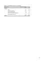
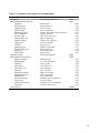
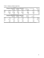
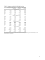
WestProPlus: A Stochastic Spreadsheet
Program for the Management of All-Aged
Douglas-fir/Western Hemlock Forests in the
Pacific Northwest
Jingjing Liang, Joseph Buongiorno, and Robert A. Monserud
Authors
Jingjing Liang is a Research Associate and Joseph Buongiorno is the Class of 1933 Bascom
Professor and John N. McGovern WARF Professor, Department of Forest Ecology and
Management, University of Wisconsin-Madison, 1630 Linden Drive, Madison, WI 53706;
Robert A. Monserud is a research forester, U.S. Department of Agriculture, Forest Service,
Pacific Northwest Research Station, 620 SW Main St., Suite 400, Portland, OR 97205.
2
Abstract
Liang, Jingjing; Buongiorno, Joseph; Monserud, Robert A. 2006. WestProPlus: a spreadsheet
program for the management of all-aged Douglas-fir/western hemlock forests in the
Pacific Northwest.
WestProPlus is an add-in program developed to work with Microsoft Excel® to simulate the
growth and management of all-aged Douglas-fir/western hemlock stands in Oregon and
Washington. Its built-in growth model was calibrated from 2,706 permanent plots in the
Douglas-fir/western hemlock forest type in Oregon and Washington. Stands are described by the
number of trees per acre in each of 19 2-inch diameter classes in four species groups: Douglasfir, other shade-intolerant species, western hemlock, and other shade-tolerant species.
WestProPlus allows managers to predict stand development by year and for many
decades from a specific initial state. The simulations are stochastic, based on bootstrapping of the
disturbances observed on the permanent plots between inventories. Users can choose cutting
regimes by specifying the interval between harvests (cutting cycle) and a target distribution of
trees remaining after harvest. A target distribution can be a reverse-J-shaped distribution or any
other desired distribution. Diameter-limit cuts can also be simulated. Tabulated and graphic
results show diameter distributions, basal area, volumes by log grade, income, net present value,
and indices of stand diversity by species and size.
This manual documents the program installation and activation, provides suggestions for
working with Excel®, and gives background information on WestProPlus’s models. It offers a
comprehensive tutorial in the form of two practical examples that explain how to start the
program, enter simulation data, execute a simulation, compare simulations, and plot summary
statistics.
Keywords: WestProPlus, simulation, growth model, Douglas-fir, western hemlock, management,
economics, ecology, diversity, wood quality, risk.
Contents
1. Introduction.........................................................................................................................................1
What Is WestProPlus?.......................................................................................................................................1
Why Simulate This Type of Stand?..................................................................................................................2
How Does WestProPlus Work?.........................................................................................................................3
What Is in This Manual?...................................................................................................................................3
2. Getting Started.....................................................................................................................................4
System Requirements........................................................................................................................................4
Loading WestProPlus.........................................................................................................................................4
Unloading WestProPlus.....................................................................................................................................6
3. Using WestProPlus..............................................................................................................................6
WestProPlus Input.............................................................................................................................................6
BDq Calculator .................................................................................................................................................8
Storing Data and Retrieving Stored Data ......................................................................................................9
Running Simulations.........................................................................................................................................9
4. Example: Simulating BDq Management Regimes.........................................................................10
Simulation Parameters....................................................................................................................................11
Running Simulations ......................................................................................................................................13
Simulation Output ..........................................................................................................................................14
Comparison of BDq Selection Regimes ........................................................................................................26
Troubleshooting WestProPlus..............................................................................................................29
Acknowledgments..................................................................................................................................30
Metric Equivalents................................................................................................................................31
Literature Cited.....................................................................................................................................32
Appendix 1—WestProPlus Plot Data..................................................................................................36
Appendix 2—Growth-and-Yield Model..............................................................................................42
Appendix 3—Log Grade Equations....................................................................................................45
Appendix 4—Stochastic Stumpage Price and Interest Rate Models................................................48
1) Assumes 0.012 ft3/Mbf. ....................................................................................................................49
Appendix 5—Definition of Diversity of Tree Species and Size..........................................................50
Glossary..................................................................................................................................................51
1
1. Introduction
The WestProPlus User’s Manual is intended to help forest managers predict the effects of management,
or lack thereof, on stand growth, productivity, income, wood quality, diversity of species, and diversity
of tree size. The WestProPlus User’s Manual documents background, instruction, and additional
suggestions for using the WestProPlus program. The next section explains how to install WestProPlus
on your computer and provides a description of the input data, as well as instructions for loading and
saving these data, running simulations, and saving the results. Examples of applications in simulating
management regimes are given. If you are new to WestProPlus, it will be useful to run these examples
while reading the manual. We included answers to some common questions. Appendices cover the
growth equations, volume equations, and log grade equations of WestProPlus, and the data used to
calibrate these equations.
The WestProPlus software and all the sample spreadsheets can be downloaded online from
http://www.forest.wisc.edu/facstaff/buongiorno/ .
What Is WestProPlus?
WestProPlus is a computer program to predict the development of all-aged Douglas-fir/western
hemlock forests in the Pacific Northwest. With this program, various management regimes can be
considered, and their outcomes can be quickly predicted. WestProPlus is a successor of WestPro
(Ralston et al. 2003). WestProPlus has the following features compared to WestPro:
1) Extensions of the database from 66 uneven-aged plots to 2,706 all-aged plots, covering most
of the Douglas-fir/western hemlock type in Oregon and Washington (App. 1).
2) Expansion of species groups from two (softwoods, hardwoods) to four (Douglas-fir, other
shade-intolerant, western hemlock, other shade-tolerant).
1
3) Calibration of an improved growth model, with particular attention to the effect of stand
diversity on growth, mortality, and recruitment (Liang et al. 2005a).
4) Introduction of log grade equations to predict the effects of management on wood quality.
5) Recognition of risk and uncertainty in stand growth, timber prices, and interest rates.
Three other deterministic relatives of WestProPlus (CalPro, NorthPro, and SouthPro) already
exist for California mixed conifer forests (Liang et al. 2004a), northern hardwoods in Wisconsin and
Michigan (Liang et al. 2004b), and for loblolly pine in the Southern United States (Schulte et al. 1998),
respectively. We have used our experience with these programs to further simplify the data input and
the program output to increase WestProPlus’ usefulness for practitioners.
Why Simulate This Type of Stand?
Douglas-fir/western hemlock (Pseudotsuga menziesii/Tsuga heterophylla) forests in the Pacific
Northwest are very productive. They were harvested heavily during the late 1800s and early 1900s, at
an unsustainable rate (Curtis and Carey 1996). Consequently, although they vary highly in composition
and structure Douglas-fir/western hemlock forests are mostly in early seral stages (Barbour and
Billings 1988).
Douglas-fir wood is valued for its superior mechanical properties, making it most useful in
building and construction (Barbour and Kellogg 1990). Western hemlock is another important
commercial species. It is shade tolerant yet fast growing, deer and elk browse it, and hemlock trees are
a part of the esthetics of western forests (Burns and Honkala 1990).
Even-aged silviculture is prevalent in managed Douglas-fir forests. There has been little
tendency to adopt uneven-aged (selection) management (Emmingham 1998) despite its attractive
features (Hansen et al. 1991; Guldin 1996). This seems to be due to a lack of experience with unevenaged management, and scarcity of data regarding its effects compared to even-aged systems.
2
WestProPlus helps predict the development of Douglas-fir-western hemlock stands with various
types of silviculture. Some of the examples in this manual suggest that effective uneven-aged
management of Douglas-fir/western hemlock forests can be profitable while maintaining stands with
high diversity of tree species and size.
How Does WestProPlus Work?
WestProPlus predictions are based on a stochastic version of a multispecies, site- and densitydependent matrix growth model (Liang et al. 2005a, App. 2), coupled with log grade model (App. 3),
stochastic stumpage price and interest rate models (App. 4). To run WestProPlus, you specify an initial
stand state, define a management policy by target stand state, and cutting cycle. The program predicts
economic and ecological effects of the policy, with a sequence of random numbers to simulate
stochastic shocks in stand growth, timber prices, and interest rates.
As you change policy, WestProPlus repeats the same sequence of random numbers to simulate
stochastic stand growth, timber prices, and interest rates. Using the same string of random numbers
facilitates comparison of management policies. A new string of random numbers may also be generated
by quitting WestProPlus and loading it again (see section 2).
What Is in This Manual?
The next section explains how to install WestProPlus on your computer and provides a description of
the input data, as well as instructions for loading and saving these data, running simulations, and
saving the results. Examples of applications in simulating uneven-aged management regimes are given.
We included answers to some common questions. Appendices cover the equations involved in
WestProPlus, and the data used to calibrate these equations. The manual assumes that you are familiar
with the basics of Microsoft Excel®. All the spreadsheets shown in this manual are screenshots from
the Excel® 2003.
3
2. Getting Started
System Requirements
You need the following hardware and software to operate WestProPlus:
A computer (PC) with at least 128 megabytes of random access memory (RAM)
Microsoft® Windows® 98, 2000, Me, XP, or Windows NT™ 41
Microsoft® Excel® 97 or above
A free copy of the WestProPlus software downloaded from
http://www.forest.wisc.edu/facstaff/buongiorno/, or from the authors through
[email protected].
Loading WestProPlus
To install the program for the first time:
1. Insert the diskette containing WestProPlus.xla into your computer, or download it from the
Web site to your local disk and go to step 3.
2. Select the WestProPlus.xla icon and copy it onto your hard disk. For your convenience, you
may save it in a new folder named WestProPlus, e.g., C:\WestProPlus\WestProPlus.xla.
3. Open Microsoft® Excel® and START A NEW WORKBOOK.
4. Under the Tools menu, select Add-ins. In the add-ins dialogue box, select Browse and choose
WestProPlus.xla from its location on your hard disk. Click OK.
5. Return to the Tools menu. WestProPlus is now the last item in the menu. Select WestProPlus
and click OK in the title box.
The use of trade or firm names in this publication is for reader information and does not imply endorsement by the U.S.
Department of Agriculture of any product or service.
1
4
6. The WestProPlus menu should now be in the Excel® menu bar.
Until you uninstall it, WestProPlus will be a permanent option in the Tools menu of Excel®. You can
load the program by selecting WestProPlus in the Tools menu. This will add WestProPlus to the
Excel® menu, and the input data worksheet (fig. 1) will appear.
Figure 1—Input data worksheet.
There are three sample workbooks at http://www.forest.wisc.edu/facstaff/buongiorno/ with the
input data worksheets corresponding to the examples in section 4 of this paper. By copying the data
from these worksheets into your input data worksheet you will be able to run these examples with
WestProPlus.
5
Unloading WestProPlus
To finish working with WestProPlus, choose the command Quit under the WestProPlus menu. The
WestProPlus menu will disappear, but the current worksheets will stay in the Excel® window until you
close them.
To remove the WestProPlus menu and uninstall the program:
1. Quit WestProPlus.
2. Under the Tools menu, select Add-ins. Deselect WestProPlus to remove the title from the addins list.
3. Close the Excel® window.
3. Using WestProPlus
WestProPlus Input
The input data worksheet (fig.1) contains all the information needed by the program. Cells with
question marks require numeric entries, except that initial timber prices are optional. WestProPlus
converts numeric entries to one or two decimal places. Before running a simulation, WestProPlus
checks all your entries and will prompt you to fix any improper input data.
In figure 1, the four rows labeled “initial state” contain the initial number of trees per acre in
the stand (at time zero), by species groups and by 2-in diameter classes. WestProPlus recognizes four
species groups: Douglas-fir, other shade-intolerant species, western hemlock, and other shade-tolerant
species (App. 1, table 3).
The four rows labeled “target state” contain the number of trees per acre that should remain
after harvest, by species group and diameter class. A target entry of zero instructs WestProPlus to
harvest all trees in that category. When the number of trees in the stand exceeds the target value, the
6
harvest is the difference between the available trees and the target; otherwise the harvest is zero. You
can avoid harvesting in any species group and size class by entering a very high target, e.g., 10,000.
You can enter the initial and target states by hand or with the BDq calculator described below.
WestProPlus measures time in years. All simulations start at time zero and last for the “Length
of the simulation.” The “Year of first harvest” may be set at any nonnegative integer value. The
“Length of cutting cycle”, i.e., the interval between harvests, must be at least 1 year. To simulate stand
growth without harvest, set the “Year of the first harvest” to a value greater than the “Length of the
simulation.”
The “Re-entry cost” represents cost of doing a harvest, in dollars per acre, independent of the
volume harvested. The cost of timber sale preparation and administration would be part of a typical reentry cost.
The “Site Productivity”, measured by mean annual increment, describes the wood-growing
capacity of a site. It is defined as the increment in volume of a timber stand averaged over the period
between age zero and the age at which mean annual increment reaches its maximum value (Hanson et
al. 2002). If you do not enter any value for Site Productivity, WestProPlus assumes that the site
productivity is 150 ft3/ac/yr, the average site productivity in the 2,706 permanent plots in Washington
and Oregon used to calibrate the growth equations of WestProPlus. The site productivity should be
between 10 to 300 ft3/ac/yr, the range of the data.
The “Site Index” was measured by the average total height of the dominant and codominant
trees at 50 years of age (Hanson et al. 2002). WestProPlus uses site index to predict log grade. The site
index should be between 30 and 99, the range of the data.
The “Interest Rate” represents the initial interest rate. Starting from this initial value,
WestProPlus generates a sequence of yearly stochastic interest rates. These interest rates are used to
calculate the net present value of each harvest, and the cumulative net present value.
7
The “Initial Timber Prices” are the initial stumpage prices by log grade and species group.
These entries are optional. If you leave these cells blank, WestProPlus will generate random initial
prices. Starting from these initial values, WestProPlus generates a sequence of stochastic prices (App.
4).
BDq Calculator
A BDq distribution is a tree distribution, by diameter class, defined by a stand basal area (B), a
maximum and minimum tree diameter (D), and a q-ratio (q), the ratio of the number of trees in a given
diameter class to the number of trees in the next larger class. You can use the BDq calculator (Schulte
et al. 1998) to define the target state or the initial state with a BDq distribution.
To use the BDq calculator, click on the BDq calculator icon in the input data worksheet. Use
the arrow buttons to set the stand basal area (ft2/ac), the q-ratio, the minimum and the maximum
diameters (in); click the Calculate button (fig. 2).
Figure 2—The BDq Distribution Calculator window.
The example in figure 2 shows the number of trees by diameter class that would give a basal
area of 120 ft2/ac with trees of diameters from 3 to 33 inches and a q-ratio of 1.3 for the Douglas-fir
trees in the initial stand state. You can copy the resulting stand distribution to the input data worksheet
8
as the initial distribution or as the target distribution for a species group by selecting the destination
and clicking the Copy button on the BDq calculator (fig. 2).
Storing Data and Retrieving Stored Data
After entering data in the Input Data worksheet, you can save this worksheet for later use. You should
save your work frequently to avoid losing data. It is advisable to save the work in a particular folder to
facilitate locating the file in the future.
To run several simulations (e.g., to examine the effects of changing some of the parameters)
you may find it efficient to work with previously saved input data. To retrieve the data, choose the File
→ Open command in Excel® to open your saved file or double click on the file icon.
Running Simulations
After completing the input data worksheet or retrieving a previously saved one, you are ready to run a
simulation. To run WestProPlus, make sure that the WestProPlus menu is in the Excel® menu bar. If
not, click WestProPlus under the Tools menu to activate WestProPlus. You can then run the simulation
by choosing Run in the WestProPlus menu.
Each WestProPlus simulation generates the following worksheets and charts:
A TreesPerAcre worksheet: The number of trees by species and diameter class for each
simulated year.
A Basal Area worksheet: The basal area by species and timber size, for each simulated year.
A Volume worksheet: The volume in stock by log grade, for each simulated year.
A Products worksheet: The physical output and the financial return from the harvests
throughout the simulation.
9
A Diversity worksheet: Shannon’s species diversity indices and size diversity indices for each
year of the simulation.
A Diversity chart: A plot of Shannon’s indices of species and size diversity over time.
A Species BA chart: A stacked area chart showing the development of stand basal area by
species group over time.
A Size BA chart: A stacked area chart showing the development of stand basal area by timber
size over time.
A Volume chart: A stacked area chart showing the development of volume in stock by log
grade over time.
To compare various management regimes, save the output worksheets immediately after
running a simulation. Otherwise WestProPlus will overwrite the previous results every time you run a
new simulation.
All the data in the output worksheets are protected and you cannot change them. To see how
results change with different input data, change the input data worksheet and rerun the simulation.
4. Example: Simulating BDq Management Regimes
In this example, we performed simulations of selection regimes based on the basal-area-diameter-qratio (BDq) principle. For a given initial state, we changed the q-ratio of the target stand state, and
interpreted the results in terms of effects on economic returns, productivity, tree diversity, wood
quality, and stand structure. We concentrate on the q-ratio because it is the main effect in most unevenaged management criteria (Liang et al. 2005b).
10
Simulation Parameters
The simulations were for 200 years, with cutting cycles of 10 years. The initial stand state was the
average distribution of the 2,706 permanent plots used in calibrating the growth equations of
WestProPlus (fig. 3). Composition by number of trees was 34% Douglas-fir, 30% other shadeintolerant species, 20% western hemlock, and 16% other shade-tolerant species. The average site
productivity was 150 ft3/ac/yr and the average 50-year site index was 90 ft.. The first harvest started at
year 1. The fixed cost of re-entry was set at $254/ac, the estimated cost of preparing and administering
timber sales in the state of Washington (Ralston et al. 2003). The initial interest rate was set at 3.8% per
year, the yield of AAA bonds net of inflation, from 1970 to 2004 (U.S. Government Printing Office,
2005). The initial stumpage prices came from Oregon stumpage prices in 2005 (Log Lines 2005, table
8).
80
Douglas-fir
Other shade-intolerant species
Western hemlock
Other shade-tolerant species
Trees/a
60
40
20
0
4
8
12
16
20
24
28
Diameter (in)
32
36
40
Figure 3—Initial stand state.
The three alternative target distributions are shown in figure 4. They all assumed a maximum
diameter of 40 in. for all species. The basal area was kept the same in the three alternatives, 87 ft2/ac in
total (Miller and Emmingham 2001), consisting of 30 ft2/ac of Douglas-fir, 26 ft2/ac of other shadeintolerant species, 17 ft2/ac of western hemlock, and 14 ft2/ac of other shade-tolerant species. The q11
ratio was set at 1.2, 1.4, or 1.8. Higher q values kept more trees in the smaller diameter classes relative
to the large (fig. 4).
Figure 4—Target distribution of trees by species groups and diameter class for the BDq regime used here.
Figure 5 shows the BDq calculator set to produce the target state for Douglas-fir trees with
basal area of 30 ft2/ac, maximum diameter of 40 in., and q-ratio of 1.2. Clicking on the Calculate
button produces the number of trees by size class.
Figure 5—BDq Distribution Calculation dialog box.
To copy the distribution of Douglas-fir to the Input Data worksheet, select the option box
corresponding to Douglas-fir Target Distribution and click on the Copy button. Figure 6 shows the
Input Data worksheet for the above BDq selection regime with q=1.2.
12
Figure 6—Input Data worksheet for the BDq selection regime with 87 ft2/ac residual basal area, 40 in.
maximum diameter, q=1.2, and ten years cutting cycle.
Running Simulations
Upon running a simulation, WestProPlus will replace any old tables and charts with new ones. For this
reason, you should save the workbook after each simulation. To run a series of simulations, load the
input data for the first management regime, run the simulation, save your outcome, and proceed to load
and run the second management regime. You can then compare the data on economic return, various
ecological criteria, and wood quality for different regimes. To that end, comparative charts and tables
can be built with Excel® from the WestProPlus output worksheets.
13
Simulation Output
The simulation outcomes of the forgoing BDq selection are displayed in tables and charts. They are
located in the same workbook as the Input Data worksheet. The following results are for the initial
condition and BDq management specified by the input data in figure 6.
TreesPerAcre worksheet— This worksheet (fig. 7) shows the number of trees per acre, by species and
diameter class, for each year of simulation. Scrolling to the right reveals the tree distribution for other
species. The underlined numbers are the year of harvest, and the number of trees per acre after the
harvest.
Basal Area Worksheet—This worksheet (fig. 8) shows, for each simulated year, the total stand basal
area, the stand basal area by species group, and the stand basal area by timber size category: poles
(trees from 5 to 11 inches DBH), small sawtimber (trees from 11 to 15 inches DBH), medium
sawtimber (trees from 15 to 21 inches DBH), and large sawtimber (trees 21 inches DBH and larger).
Underlined numbers show the year of harvest and the basal areas just after harvest, and the first row
represents the average basal area.
Volume worksheet— This worksheet (fig. 9) shows the volume in stock by log grade. The log grade
equations used by WestProPlus are described in appendix 3. The underlined numbers represent the year
of harvest and the volume per acre just after the harvest, and the first row represents the average
volume.
14
Products Worksheet—The upper part of the products worksheet (fig. 10) shows data for each harvest:
basal area cut, volume harvested by log grade, gross income, predicted net present value (NPV) of the
current harvest, the total (cumulative) NPV, and the initial stock value. The log grade equations, and
the stochastic stumpage price model and interest rate model used by WestProPlus are described in
appendix 3 and 4.
The lower part of the products worksheet shows the average annual cut and the average stock in
terms of basal area and volume by log grade. It also displays the average species diversity and size
diversity.
The results show that with this particular BDq selection and a 10-year cutting cycle, the average
yield over 200 years would be 71.06 ft3/ac/yr, for a net present value of $16378.33/ac. This is the value
of the land and initial trees, under this management. It suggests that this regime would be economically
efficient. Because the value of the initial trees was $11959.13/ac, the present value of the return from
land and initial trees would exceed the initial investment in trees.
Diversity Worksheet—The diversity worksheet (fig. 11) shows Shannon’s indices of species group
diversity and tree size diversity for each simulated year (see App. 5 for the definitions of Shannon’s
diversity). The underlined data show the year of harvest and the values of the diversity indices just
after harvest. The boldfaced values represent the average diversity indices of all years.
Diversity Chart—The Diversity Chart (fig. 12) displays the evolution of Shannon’s indices over time.
The results show that the effect of stochasticity in forest growth is greater than the effect of harvests on
the species and size diversity.
15
Species BA Chart—This chart (fig. 13) shows the development of basal area by species throughout the
simulation period. The chart shows the sharp decrease of total basal area is due to the periodic harvests.
It also suggests that in the long run this management would sustain all four species groups in the stand.
Timber Size BA Chart—This chart (fig. 14) shows the development of basal area by timber size
throughout the simulation. It excludes the basal area of trees smaller than poles (less than 5 inches in
diameter). The results suggest that all the four size groups would remain present in the stand for 200
years. The basal area of large sawtimber would tend to increase over time with this management.
Volume Chart—This chart (fig. 15) shows the development of volume in stock by log grade
throughout the simulation period. The chart suggests that all log grades would continue to be present in
the stand. The stock of peeler, and #1 Sawmill logs tended to increase slightly over time under this
management.
16
Figure 7—TreePerAcre worksheet for the BDq selection regime with 87 ft2/ac residual basal area, 40 in.
maximum diameter, q=1.2, and ten years cutting cycle.
17
Figure 8—Basal Area worksheet for the BDq selection regime with 87 ft2/ac residual basal area, 40 in.
maximum diameter, q=1.2, and ten years cutting cycle.
18
Figure 9—Volume worksheet for the BDq selection regime with 87 ft2/ac residual basal area, 40 in. maximum
diameter, q=1.2, and ten years cutting cycle.
19
Figure 10—Products worksheet for the BDq selection regime with 87 ft2/ac residual basal area, 40 in.
maximum diameter, q=1.2, and ten years cutting cycle.
20
Figure 11—Diversity worksheet for the BDq selection regime with 87 ft2/ac residual basal area, 40 in.
maximum diameter, q=1.2, and ten years cutting cycle.
21
Figure 12—Diversity chart for the BDq selection regime with 87 ft2/ac residual basal area, 40 in. maximum
diameter, q=1.2, and ten years cutting cycle.
22
Figure 13—Species Basal Area chart for the BDq selection regime with 87 ft2/ac residual basal area, 40 in.
maximum diameter, q=1.2, and ten years cutting cycle.
23
Figure 14—Timber Size BA chart for the BDq selection regime with 87 ft2/ac residual basal area, 40 in.
maximum diameter, q=1.2, and ten years cutting cycle.
24
Figure 15—Volume chart for the BDq selection regime with 87 ft2/ac residual basal area, 40 in. maximum
diameter, q=1.2, and ten years cutting cycle.
25
Comparison of BDq Selection Regimes
As an example of how WestProPlus can be used to compare managements, follow the steps below to
compare BDq selection regimes with a ten-year cutting cycle, 87 ft2/ac residual basal area, 40 in.
maximum diameter, and a q-ratio of 1.2, 1.4, or 1.8:
1) Load WestProPlus, fill in, and save three input data worksheets corresponding to the three qratios,
2) Run a simulation for each input data worksheet and record the total net present value ($/ac),
productivity (ft3/ac/yr), average stand diversity of tree species and size, average basal area, and
average percent of peeler logs from the products worksheet (fig. 10),
3) Keep the three input data worksheets active on the desktop and quit WestProPlus (see
section 2),
4) Reload WestProPlus (see section 2) and go to step 2 to start a new replication.
WestProPlus did three simulations in step 2 for the three regimes with the same string of
random numbers to compare the regimes efficiently, while steps 3 and 4 generate a new string of
random numbers for another replication.
An example of ten replications is in table 1. There was a strong positive effect of q-ratio on the
productivity (fig. 16), because more large trees were cut with higher q-ratios. As smaller trees were left
on the stand, higher q-ratio leads to significantly lower percentage of peelers, and lower tree size
diversity. Here, we have detected little or no effect of q-ratio on the other criteria with only ten
replications. More replications with more initial states suggest that as the q-ratio increases, NPV
increases, species diversity decreases, and basal area increases (Liang et al. 2005b).
26
Table 1—Simulation results of the three BDq selection regimes with different q-ratios
NPV ($/ac)
q=1.4
19443
12551
11049
11689
13045
14463
29217
7337
14459
20924
Replication
1
2
3
4
5
6
7
8
9
10
q=1.2
14133
10375
9572
9349
9710
11153
20804
5917
12656
17656
1
2
3
4
5
6
7
8
9
10
Species diversity
q=1.2
q=1.4
1.33
1.32
1.33
1.34
1.33
1.34
1.32
1.32
1.32
1.32
1.31
1.33
1.32
1.32
1.32
1.34
1.34
1.35
1.33
1.33
q=1.8
32168
21600
18441
20079
21939
23201
50303
14764
22195
33917
Productivity (ft3/ac/yr)
q=1.2
q=1.4
69.25
83.12
80.55
99.61
69.77
92.43
71.76
89.23
73.08
92.42
76.51
90.17
73.6
97.06
66.73
85.69
78.26
96.83
71.53
86.81
q=1.8
117.18
141.09
141.28
129.14
137.2
128.73
155.06
132.58
136.24
127.95
q=1.8
1.33
1.32
1.34
1.32
1.3
1.32
1.31
1.33
1.35
1.33
q=1.2
2.85
2.85
2.85
2.85
2.86
2.86
2.86
2.85
2.86
2.85
Size diversity
q=1.4
2.79
2.78
2.77
2.78
2.78
2.79
2.77
2.79
2.78
2.78
q=1.8
2.43
2.42
2.39
2.42
2.4
2.42
2.39
2.41
2.42
2.4
Percentage of peeler
q=1.2
q=1.4
q=1.8
1
0.29
0.23
0.17
2
0.3
0.22
0.17
3
0.3
0.22
0.16
4
0.31
0.22
0.16
5
0.29
0.22
0.16
6
0.32
0.23
0.16
7
0.29
0.22
0.16
8
0.31
0.22
0.17
9
0.29
0.22
0.16
10
0.3
0.22
0.16
Note: Except for NPV, all data are averages over 200 years.
Average basal area (ft2/ac)
q=1.2
q=1.4
q=1.8
75.8
79.2
74
79.6
88.5
86
74.4
86.5
85.4
74.3
83.8
79.2
77.9
86.2
82.9
73.4
81.8
79.4
76.5
88.7
91.5
73.9
83.4
84.5
79.6
87.1
81.3
74
81.7
79.2
27
40000
NPV($/a)
150
120
30000
90
20000
60
10000
30
0
0
1.2
1.5
productivity (ft3/a/y)
1.4
q-ratio
1.8
Species diversity
1.2
3
1.4
q-ratio
1.8
1.4
q-ratio
1.8
1.4
q-ratio
1.8
Size diversity
2.8
1.4
2.6
2.4
1.3
2.2
1.2
2
1.2
0.4
1.4
q-ratio
1.8
% of peeler
1.2
90
0.3
80
0.2
70
0.1
Basal area
(ft2/a)
60
1.2
1.4
q-ratio
1.8
1.2
Figure 16—Mean and standard error of the management criteria over 10 replications for different q-ratios,
other things being held constant.
28
Troubleshooting WestProPlus
Why can’t I open WestProPlus?
First, make sure you have the latest version of WestProPlus(2005). Check our website:
http://www.forest.wisc.edu/facstaff/buongiorno/ for updates.
Set your Excel® macro security level to Medium. You can change the level at Tools→ Macro→
Security. After setting the macro security level to Medium, each time you load WestProPlus, a
security warning message window will pop up, and you should select Enable Macros (fig. 17).
Figure 17—Microsoft® Excel® Security Warning Window against Macro viruses.
WestProPlus does not insert a new input data worksheet. What can I do?
Before inserting a new input data worksheet, WestProPlus checks to see if there is a worksheet named
Input Data already open. If there is one, WestProPlus will not generate a new input data worksheet. To
get a new input data worksheet, close all Excel® windows and reopen WestProPlus.
Why is there no BDq calculator in the example worksheets?
29
The example workbooks contain only the input data. After you have installed WestProPlus, the BDq
calculator icon will appear in the new input data worksheet. At that point, you can copy data from the
example workbooks into the input data worksheet.
Why is the BDq calculator not working?
WestProPlus must be open to use the BDq calculator. To use the BDq calculator on a previously saved
input data worksheet, WestProPlus must be in the Excel® menu bar.
Why can’t I copy all the content from the example worksheet to the input data worksheet?
All the cells of the input data worksheet are protected except those that need entries (marked with ?
marks). Copy only the data from the example worksheet and paste them to the corresponding locations
in the input data worksheet.
For further assistance, or to send us your comments, please contact us through [email protected].
Acknowledgments
We thank Dean Parry, Karen Waddell, and Susan Stevens Hummel for assistance with the data. The
research leading to this program was supported, in part, by the USDA Forest Service, Pacific
Northwest Research Station, by USDA-CSREES grant 2001-35108-10673, and by the School of
Natural Resources, University of Wisconsin-Madison. The authors take sole responsibility for any
error or omission.
30
Metric Equivalents
When you know:
inches (in)
feet (ft)
square feet (ft2)
square feet per acre (ft2/ac)
cubic feet (ft3)
cubic feet per acre (ft3/ac)
Multiply by:
0.3937
0.3048
0.0929
4.3562
35.3147
14.2913
To find:
centimeters (cm)
meters (m)
square meters (m2)
square meters per hectare (m2/ha)
cubic meters (m3)
cubic meters per hectare (m3/ha)
31
Literature Cited
Barbour, M.G.; Billings, W.D. 1988. North American Terrestrial Vegetation. Cambridge University
Press, Cambridge, UK. 421p.
Barbour, R.J.; Kellogg, R.M. 1990. Forest management and end-product quality: a Canadian
perspective. Can. J. For. Res. 20: 405–414.
Barbour, R.J.; Parry, D.L. 2001. Log and lumber grades as indicators of wood quality in 20- to 100year-old Douglas-fir trees from thinned and unthinned stands. General Technical Report 510, USDA
Forest Service, Pacific Northwest Research Station, Portland. 22 p.
Burns, R.M.; Honkala, B.H. (tech. coords.) 1990. Silvics of North America: 1. Conifers. USDA Agric.
Handb. 654. 675 p.
Curtis, R.O.; Carey, A.B. 1996. Managing Economic and Ecological Values in Douglas-Fir Forests. J.
For. 94: 1-7, 35-37.
Efron, B.; Tibshirani, R.J. 1994. An Introduction to the Bootstrap. CRC Press, Boca Raton, FL. 456 p.
Emmingham, W. 1998. Uneven-aged management in the Pacific Northwest. J. For. 96(7): 37-39
Guldin, J.M. 1996. The role of uneven-aged silviculture in the context of ecosystem management. W. J.
Appl. For. 11(1): 4-12.
32
Hanson, E.J. ; Azuma, D.L.; Hiserote, B.A. 2002. Site index equations and mean annual increment
equations for the Pacific Northwest Research Station Forest Inventory and Analysis, 1985-2001. Res.
Note PNW-RN-533. Portland, OR: U.S. Department of Agriculture, Forest Service, Pacific Northwest
Research Station. 24 p.
Hansen, A.J.; Spies, T.A.; Swanson, F.J.; Ohmann, J.L. 1991. Conserving biodiversity in managed
forests: lessons from natural forests. BioScience 41(6): 382-292.
Hiserote, B.; Waddell, K. 2003. The PNW-FIA integrated database user guide. A database of forest
inventory information for California, Oregon and Washington, V 1.3. FIA PNW Station, Portland,
Oregon. 10 p.
Liang, J.; Buongiorno, J.; Monserud R.A. 2005a. Growth and yield of all-aged Douglas-fir/western
hemlock forest stands: a matrix model with stand diversity effects. Can. J. For. Res. 35(10): 23692382.
Liang, J.; Buongiorno, J.; Monserud R.A. 2005b. Bootstrap simulation and response surface
optimization of management regimes for Douglas-fir/western hemlock stands. For. Sci. (In review).
Liang, J.; Buongiorno, J.; Monserud R.A. 2004a. CalPro: A spreadsheet program for the management
of California mixed-conifer stands. USDA Forest Service, Pacific Northwest Research Station, General
Technical Report PNW-GTR-619. 32p.
33
Liang, J.; Buongiorno, J.; Kolbe, A.; Schulte, B. 2004b. NorthPro: a spreadsheet program for the
management of uneven-aged northern hardwood stands. Madison, WI: University of WisconsinMadison, Department of Forest Ecology and Management. 36 p.
Miller, M.; Emmingham, B. 2001. Can selection thinning convert even-aged Douglas-fir stands to
uneven-aged structures? Western Journal of Applied Forestry 16(1): 35-43.
Northwest Log Rules Advisory Group. 1998. Official log scaling and grading rules. 8th ed. Eugene, OR.
48 p.
Oregon Department of Forestry. 2005. Quarterly Douglas-fir stumpage prices online: http:// www. odf.
state. or. us.
Ralston, R.; Buongiorno, J.; Schulte, B.; Fried, J. 2003. WestPro: a computer program for simulating
uneven-aged Douglas-fir stand growth and yield in the Pacific Northwest. Gen. Tech. Rep. PNW-GTR574. Portland, OR: U.S. Department of Agriculture, Forest Service, Pacific Northwest Research
Station. 25 p.
Schulte, B.; Buongiorno, J.; Lin, C.R.; Skog, K. 1998. SouthPro: a computer program for managing
uneven-aged loblolly pine stands. Gen. Tech. Rep. FPL-GTR-112. Madison, WI: U.S. Department of
Agriculture, Forest Service, Forest Products Laboratory. 47 p.
34
Stevens, J.A.; Barbour, R.J. 2000. Managing the stands of the future based on the lessons of the past:
estimating western timber species product recovery by using historical data. USDA For. Serv. Res.
Note PNW-RN-528. 9 p.
U.S. Government Printing Office [US GPO]. 2005. Economic report of the President. Washington, DC.
335 p.
35
Appendix 1—WestProPlus Plot Data
The data to calibrate the stand growth model used by WestProPlus came from the PNW-FIA Integrated
Database (Version 1.2) (Hiserote and Waddell, 2003), specifically, the part of the database that
combines information from four different forest inventories (FIAEO, FIAWO, FIAEW, FIAWW)
conducted by the USDA Forest Service between 1988 and 2000.
The 2,706 plots used in calibrating WestProPlus had all been classified in the Douglasfir/western hemlock forest type, they had been measured at two successive inventories, and they were
located in Oregon and Washington west of 120° in longitude (fig. 18). This area includes the Coast
Range and the Cascades Range of western Washington and Oregon, as well as the Klamath region of
southwestern Oregon. About 80% of the plots were on private land, and most of the remaining 20%
were on lands belonging to the States of Oregon or Washington (table 2). U.S. Federal lands (e.g.,
National Forests, National Parks, and Bureau of Land Management forests) are not included in this
database.
The trees were categorized into four species classes (table 3): Douglas-fir, other shadeintolerant species, western hemlock, and other shade-tolerant species (Barbour and Billings 1988). Red
alder (Alnus rubra) and ponderosa pine (Pinus ponderosa) were the most abundant shade-intolerant
species other than Douglas-fir. Western redcedar (Thuja plicata) and bigleaf maple (Acer macrophyllum)
were the most abundant shade-tolerant species other than western hemlock (table 3). Within each
species, trees were grouped into nineteen 2 in. diameter classes, from 3 to 5 in. up to 40 in. and above.
The plot characteristics are summarized in table 4. The theoretical maximum species diversity
is ln(4)=1.39, and the maximum size diversity is ln(19)=2.94, occurring when all the basal area is
equally distributed in all 4 species classes and 19 size classes, respectively. There was a 0.90
correlation between the diversity by species group, used here, and the diversity by individual species.
The average recruitment was highest for Douglas-fir and other shade-intolerant trees (table 4).
36
The individual tree data (table 5) show that, on average, Douglas-fir trees had the highest
diameter growth rate, and lowest mortality rate. Other shade-tolerant species had the highest single tree
gross volume. Although the time between measurements was short, averaging a decade, there was
much difference in trees and stand conditions between plots. It is this cross-sectional variation that
allows inferring how stands would grow in very different conditions that might arise in space and over
long time periods.
Figure 18—Geographic distribution of the FIA plots used to calibrate the growth and yield model.
37
Table 2—Distribution of plots by ownership
Ownership
Number of plots
Private
2136
Public
State
438
Local Government
67
Other federal owner
29
Bureau of Land Management
20
National Park Service
16
Total
2706
%
78.9
16.2
2.5
1.1
0.7
0.6
100.0
38
Table 3—Frequency of tree species in all sample plots
Common Name
Douglas-fir
Other Shade-intolerant Species
Red alder
Ponderosa pine
Lodgepole pine
Western larch
Black cottonwood
Pacific madrone
Incense-cedar
Oregon white oak
Western juniper
Oregon ash
Noble fir
Quaking aspen
Western white pine
Sugar pine
Jeffrey pine
Western hemlock
Other Shade-tolerant Species
Western redcedar
Bigleaf maple
Grand fir
Sitka spruce
Pacific silver fir
White fir
Mountain hemlock
Engelmann spruce
Subalpine fir
Port-Orford-cedar
Pacific yew
Alaska yellowcedar
Redwood
All the species
Scientific Name
Pseudotsuga menziesii
%
41.27
24.07
Alnus rubra
10.85
7.10
1.94
0.92
0.72
0.63
0.44
0.42
0.26
0.25
0.18
0.15
0.14
0.05
0.01
Pinus ponderosa
Pinus contorta
Larix occidentalis
Populus balsamifera ssp.trichocarpa
Arbutus menziesii
Calocedrus decurrens
Quercus garryana
Juniperus occidentalis
Fraxinus latifolia
Abies procera
Populus tremuloides
Pinus monticola
Pinus lambertiana
Pinus jeffreyi
Tsuga heterophylla
18.80
15.86
Thuja plicata
5.88
3.09
2.09
1.44
1.32
0.94
0.42
0.34
0.17
0.12
0.03
0.02
0.01
Acer macrophyllum
Abies grandis
Picea sitchensis
Abies amabilis
Abies concolor
Tsuga mertensiana
Picea engelmannii
Abies lasiocarpa
Chamaecyparis lawsoniana
Taxus brevifolia
Chamaecyparis nootkatensis
Sequoia sempervirens
100.00
39
Table 4—Summary statistics for plot data
Trees/ac
Douglas-fir Other shade
Western Other shadeSite Productivity Inter inventory
Basal area
intolerant
hemlock
tolerant
(ft3 /ac/yr)
(yr)
(ft2 /ac)
Mean
119.01
86.38
62.42
56.79
41.24
149.59
10.53
S.D.
74.23
121.74
105.75
119.63
87.59
72.17
0.90
Max
418.66
1246.45
1982.99
1223.36
1056.16
300.00
23.00
Min
2.40
0.00
0.00
0.00
0.00
10.00
9.00
n
2706
2706
2706
2706
2706
2706
2706
Recruitment (tree/ac/yr)
Species
Size
Douglas-fir Other shade
Western Other shade
diversity
diversity
intolerant
hemlock
tolerant
Mean
2.22
1.55
1.34
1.01
0.54
1.65
4733.54
S.D.
7.32
6.35
5.67
4.48
0.39
0.63
3588.06
Max
103.87
165.25
96.76
96.37
1.38
2.76
22122.76
Min
0.00
0.00
0.00
0.00
0.00
0.00
28.15
n
2706
2706
2706
2706
2706
2706
2706
Note: Level variables are at the time of the first inventory, recruitment is between the two inventories.
40
Table 5—Summary statistics for individual tree data
Douglas-fir Other shadeWestern Other shadeintolerant
hemlock
tolerant
Diameter (in)
Mean
15.28
12.01
12.97
16.06
S.D.
8.39
6.33
7.69
10.69
Max
81.81
51.42
68.37
119.90
Min
1.57
1.57
1.57
1.57
N
23161
11831
11612
8900
Diameter growth (in/yr)
Mean
0.28
0.18
0.23
0.23
S.D.
0.17
0.14
0.15
0.17
Max
5.50
6.47
3.77
3.33
Min
0.00
-0.11
0.00
-0.45
n
23161
11831
11612
8900
-1
Mortality Rate (y )
Mean
0.003
0.006
0.003
0.004
S.D.
0.016
0.023
0.017
0.019
Max
0.111
0.111
0.111
0.111
Min
0.000
0.000
0.000
0.000
n
23838
12650
12007
9295
3
Volume (ft /tree)
Mean
77.69
39.55
61.09
83.34
S.D.
99.59
51.91
90.41
154.33
Max
1986.80
790.70
1353.26
5826.92
Min
0.35
0.35
0.35
0.00
n
23161
11831
11612
8900
Note: Diameter and volume are at the time of the first inventory, diameter growth and mortality rate are
between the two inventories.
41
Appendix 2—Growth-and-Yield Model
The growth model of WestProPlus has the following form (Liang et al., 2005a):
yt
1
Gy t
r ut
(1)
1
where yt=[yijt] is the number of trees per unit area of species group i, and diameter class j, at time t. i=1
for Douglas fir, 2 for other shade intolerant species, 3 for western hemlock, and 4 for other shadetolerant species. The matrix G and the vector r are defined as:
a i1
bi 1
G1
G2
G
,G i
G3
G4
r
r1
r2
r3
r4
,
ri
a i2
⋱
⋱
bi,17
ai,18
bi ,18
ai,19
ri
0
⋮
0
where aij is the probability that a tree of species i and diameter class j stays alive and in the same
diameter class between t and t+1, bij is the probability that a tree of species i and diameter class j stays
alive and grows into diameter class j+1, and ri is the number of trees of species group i recruited in the
smallest diameter class between t and t+1, with a time period of one year. The vector ut+1 represents the
stochastic part of growth. ut+1 is bootstrapped each year from the set of vector differences between the
observed and the deterministically predicted stand state, for each of the 2,706 plots in Oregon and
Washington (Liang et al. 2005b). The bij probability is equal to the annual tree diameter growth, gij
(in/yr), divided by the width of the diameter class. Diameter growth is a function of tree diameter Dj
(in), stand basal area B (ft2/ac), site productivity Q (ft3/ac/yr), tree species diversity Hs, and tree size
diversity Hd.
42
g1 j
0.3094 0.0124 D j
0.0001D 2j
0.0010B 0.0007Q 0.0259 H s
0.0955H d
g2j
0.2403 0.0038 D j
0.0001D 2j
0.0007 B 0.0005Q 0.0278H s
0.0273H d
g3 j
0.3553 0.0148D j
0.0003D 2j
0.0010B 0.0002Q 0.0098H s
0.0689 H d
g4j
0.2304 0.0081D j
0.0001D 2j
0.0008 B 0.0005Q 0.0506H s
0.0568H d
The expected recruitment ri (trees/ac/yr) of species i is represented by a Tobit model:
(βi xi /
ri
i )βi x i
i
(βi x i /
i)
with:
β1 x1
8. 8824 0.1211B 0.0971N1
β2 x 2
β3 x 3
9.5715 0.0773B 0.0975 N 2
12.508 0.0872 B 0.0926 N 3
0.0058Q 3.4070H s
0.0190Q 5.9506 H s
2.4200 H d
4.0100 H d
β4 x 4
13.987 0.0700B 0.0924 N 4
0.0209Q 3.2546 H s
0.9200 H d
0.0227Q 4.5033H s
where Ni is the number of trees per acre in species group i; Φ and
2.7500H d
are respectively the standard
normal cumulative and density functions, and the standard deviations of the residuals are, σ1 =9.5366,
σ2 =9.0863, σ3 =11.0664, σ4 =9.3270.
The probability of tree mortality per year, mij, is a species-dependent probit function of tree size
and stand state:
m1
m2
m3
m4
1
10.5
1
10.5
1
10.5
1
10.5
( 2.1103 0.0905 D j
0.0012 D j
2
0.0019 B 0.0014Q 0.0059 H s
0.5110 H d )
( 1.4063 0.0519 D j
0.0010 D 2j
0.0012 B 0.0010Q 0.0022 H s
0.1411 H d )
( 3.1746 0.1057 D j
0.0019 D j
2
0.0036B 0.0016Q 0.3252 H s
0.4192 H d )
( 1.5188 0.0236 D j
0.0002 D j
2
0.0010 B 0.0021Q 0.2721H s
0.3528 H d )
The probability that a tree stays alive and in the same size class from t to t+1 is, then:
aij=1-bij-mij
43
The expected single tree volume vij (ft3) is a species-dependent function of tree and stand
characteristics:
v1 j
0.01712 0.00013D j
0.00001D 2j
0.00161B 0.01174 Q 0.00350 H s
0.00092 H d
v2 j
0.01536 0.00004 D j
0.00000 D 2j
0.00054 B 0.00691Q 0.00038H s
0.00100H d
v3 j
0.01294 0.00016 D j
0.00001D 2j
0.00087 B 0.00416Q 0.00185 H s
0.00145H d
v4 j
0.00392 0.00019 D j
0.00000 D 2j
0.00105B 0.00584Q 0.00692 H s
0.00035 H d
44
Appendix 3—Log Grade Equations
The equation to predict log grade were calibrated with data from 3,378 logs in the USFS Product
Recovery Database (Stevens and Barbour 2000). The logs are classified into five grade categories,
according to their diameter, branch size, growth rate, and minimum length (Barbour and Parry 2001,
Northwest Log Rules Advisory Group 1998). For WestProPlus, the logs were divided into the four
species groups recognized by the growth model (App. 2).
In addition to the log grade, the diameter of the logs was known for all species groups. The
database also contains information on the stands from which the logs were taken. However, for
Douglas-fir and western hemlock, only the tree diameter D (in) and the site index S (ft) influenced log
grade significantly (Liang et al. 2005b).
The log grade was predicted with a logistic regression and a nominal response variable:
ln
ijl
il
ilD
D
ilS
S
ijm
where πijl/πijm was the ratio between the probability of log grade l (l=1, 2, …, m-1), and log grade m,
for species i and diameter class j. The parameters, βil, of the log grade equation for Douglas-fir and
western hemlock are in table 6. For both species, log grade was higher for larger trees on less
productive sites.
There was no data on stand characteristics for other shade-tolerant and shade-intolerant species,
and no systematic relation was observed between grade and diameter for these species groups.
WestProPlus uses the observed percentages of total volume by log grade for each diameter class, and
assumes that they are constant (table 7).
45
Table 6—Estimation results of the nominal-logistic equations of log grade
Dependent Independent
Coefficient
SE
P
variable
variable
Douglas-fir
π1/ π4
Constant
2.91
1.20
0.02
D
0.02
0.00
0.00
S
-0.33
0.10
0.00
π3/ π4
Constant
1.66
1.43
0.25
D
0.02
0.00
0.00
S
-0.33
0.13
0.03
Western hemlock
π1/ π4
Constant
-8.94
4.28
0.04
D
0.16
0.02
0.00
S
-1.33
0.50
0.03
π2/ π4
Constant
-8.37
4.04
0.04
D
0.14
0.02
0.00
S
-1.00
0.43
0.07
π3/ π4
Constant
-5.90
1.59
0.00
D
0.10
0.01
0.00
S
-0.43
0.13
0.00
πl=probability of log grade l (no Douglas-fir log was observed of grade 2, grade 5 was not observed
for both species),
D=tree diameter,
S=site index,
P =level at which the effect of the control variable would be just significant.
46
Table 7—Percentage of timber volume by log grade (I through V) and size for the shadeintolerant species except Douglas-fir, and the shade-tolerant species except western hemlock.
Diameter
(in)
4
6
8
10
12
14
16
18
20
22
24
26
28
30
32
34
36
38
40
Other shade-intolerant species (%)
I
II
III
IV
V
0
0
0
0
0
0
0
0
0
0
0
0
0
100
0
0
20
0
80
0
0
24
0
76
0
0
23
10
66
0
0
16
59
25
0
0
20
69
7
4
0
16
78
6
0
0
21
79
0
0
0
14
77
4
5
6
27
64
3
0
7
33
58
2
0
19
43
36
2
0
21
43
29
0
7
13
69
13
0
6
0
70
20
0
10
0
40
60
0
0
0
75
25
0
0
Other shade-tolerant species (%)
I
II
III
IV
V
0
0
0
0
0
0
30
0
58
12
0
30
0
66
4
0
37
0
61
1
0
35
0
64
1
0
33
12
55
0
0
28
50
20
2
0
36
47
16
1
0
36
48
11
4
0
29
60
9
2
0
37
50
11
2
1
26
66
6
1
1
40
52
6
1
1
32
56
7
4
3
42
50
5
0
0
44
52
4
0
0
44
48
8
0
8
62
31
0
0
0
43
50
0
7
47
Appendix 4—Stochastic Stumpage Price and Interest Rate Models
The stumpage price model in WestProPlus (Liang et al. 2005b) was calibrated with quarterly stumpage
prices of Douglas-fir grade I logs from 1977 to 2003 in Oregon (Oregon Department of Forestry,
2005). The following autoregressive-moving average model was used to represent quarterly price
changes:
Pt
1
0.60 Pt
0.05et
et
1
(3)
where Pt and Pt-1 were stumpage prices at quarter t and quarter t-1, respectively, and et was a whitenoise residual error. The parameters were estimated from the data with the Box-Jenkins method.
WestProPlus simulates stochastic price series with this model by bootstrapping, i.e., by drawing
randomly with replacement at each step t a pair of shocks et and et+1 from the residuals obtained by
fitting model (3) to the data.
The initial price of Douglas-fir grade I logs is equal to that entered by the user (fig. 1), or
lacking this, it is bootstrapped from the prices observed from 1977 to 2003. With bootstrapped initial
prices, the mean predicted stumpage prices of Douglas-fir grade I logs and its standard error over 500
replications of 100-year simulations had a slight positive trend over time, but it was not statistically
significant.
The price of logs of other grades than grade I is calculated according to the relative prices
entered by the user (fig. 1), or lacking this, according to the relative prices in table 8. In either case, the
relative prices are constant over time.
The annual rate of return of AAA bonds from 1970 to 2004 (U.S. Government Printing Office,
2005) was used as the interest rate. WestProPlus uses an autoregressive model of interest rates:
rt
1
0.72 0.81rt
t
(4)
48
where rt was the interest rate at year t, and εt was the white-noise residual. WestProPlus
simulates stochastic interest rates by bootstrapping: at each step t, a shock was drawn randomly with
replacement from the sample of the residuals obtained by fitting the model to the data. With
bootstrapped initial interest rate, the mean predicted interest rate over 500 simulations showed no trend
over time.
Table 8—Stumpage prices ($/ft3)1 in Oregon by log grade and species group in 2005 (Log Lines
2005)
Log
Grade
I
II
III
IV
V
Douglas-fir
9.18
5.58
5.22
4.68
0.60
Other Shadeintolerant Species Western hemlock
6.60
3.30
6.48
3.24
5.28
2.94
4.50
2.46
0.60
0.60
Other Shadetolerant Species
7.80
7.50
7.50
7.50
0.78
1) Assumes 0.012 ft3/Mbf.
49
Appendix 5—Definition of Diversity of Tree Species and Size
WestProPlus uses Shannon’s index to measure the stand diversity in terms of tree species (how
uniformly trees are distributed across species groups), and timber size classes. WestProPlus measures
the presence of trees in a class by their basal area, which gives more weight to larger trees.
The tree species diversity is defined in WestProPlus as:
m
H species
i 1
yi
y
ln i
y
y
where yi is the basal area of trees of species group i per acre, and y is total basal area. In WestProPlus,
m = 4 (there are four species groups). The tree species diversity has a maximum value of ln(4) = 1.39,
when basal area is equally distributed in the four species groups, and a minimum value of zero when all
trees are in the same species group.
Similarly, tree size diversity is:
H size
n
j 1
yj
y
ln
yj
y
where yj is the basal area of trees in diameter class j per acre. In WestProPlus, n = 19 diameter classes.
The tree size diversity has a maximum ln(19) = 2.94 when basal area is equally distributed in all 19
diameter classes, and a minimum of zero when all trees are the same diameter class.
50
Glossary
BA chart—A WestProPlus-generated chart showing, for a selected range of years, the per acre basal area of
softwoods, hardwoods, and the whole stand.
BDq distribution—A tree distribution, by diameter class, defined by a stand basal area (B), a maximum and
minimum tree diameter (D), and a q-ratio (q), the ratio of the number of trees in a given diameter class to
the number of trees in the next larger class.
bootstrap method—When used in stochastic simulations, this technique simulates random variables by
sampling randomly (with replacement) from actual observations of the variable, rather than from an
assumed distribution. See Efron and Tibshirani 1994 for the details.
cutting cycle—The number of years between successive harvests. For two-cut silvicultural systems, this is the
number of years between the two harvests.
diameter class—One of 19 2-in diameter at breast height (DBH) categories used by WestProPlus to classify
trees by size. Diameter classes range from 4 to 40+ inches, with each class denoted by its midpoint
diameter. Diameter class 4 is for trees with diameters from 3 to less than 5 inches. The 40+ inch class is
for all trees 39 inches in diameter and larger.
Diversity chart—A WestProPlus-generated chart showing changes in the Shannon index of species or size
diversity over a selected range of years.
initial stand state—The number of live trees per acre, by species and size, at the start of a simulation.
input data worksheet—A worksheet to enter the data for running a WestProPlus simulation.
Log grade— An estimate of the type and quality of lumber recovered when the log is sawed.
Microsoft® Excel® add-in—A command, function, or software program that runs within Microsoft® Excel®
and adds special capabilities. WestProPlus is an add-in.
net present value (NPV)—The net revenue discounted to the present.
preharvest stand state—The number of live trees per acre, by species and size, immediately before a harvest.
Products worksheet—A WestProPlus output worksheet that shows, for each harvest, the basal area cut, the
volume of poles and sawtimber removed by species group, the gross income generated, and the net present
value of the harvest, as well as the total net present value of the stand and its mean annual production in
terms of basal area cut and volumes harvested, on a per acre basis.
pole-size trees—Trees suitable for the production of poletimber but too small to produce saw logs. In
WestProPlus, these include trees from 5 to less than 11 inches.
re-entry costs—Costs per acre associated with each harvest that are not reflected in the stumpage prices.
These may include, e.g., the added expense of marking the stand for single-tree selection or controlling
hardwood competition.
51
sawtimber—Trees suitable for the production of saw logs. WestProPlus’s marking guides recognize three
classes of sawtimber trees:
(1) Small sawtimber—Trees with diameters of 11 to less than 15 inches.
(2) Medium sawtimber—Trees with diameters of 15 to less than 21 inches.
(3) Large sawtimber—Trees with diameters of 21 inches or larger.
Setup File worksheet—A worksheet to store WestProPlus setup files. It is typically hidden.
Setup Files—Collections of related input data that are stored together on a Setup File worksheet. Setup Files
may contain data for initial stand states, target stand states, cutting cycle parameters, stumpage prices, or
fixed costs, and may be used in varying combinations as input for WestProPlus simulations.
site index—The average height of a stand’s dominant and codominant trees at age 50 years.
size diversity—The diversity of tree diameter classes as measured by the Shannon index. With 19 diameter
classes, size diversity reaches its maximum value of 2.94 when the basal area or number of trees is
distributed evenly among the diameter classes.
species diversity—The diversity of species groups as measured by the Shannon index. With four species
classes, species diversity reaches its maximum value of 1.39 when the basal area or number of trees is
distributed evenly among the species groups.
species groups—The four categories used by WestProPlus to classify trees by species. For a complete list of
species, see Liang et al. 2005a.
Douglas-fir—Pseudotsuga menziesii.
Other shade-intolerant species—Including Alnus rubra, Pinus ponderosa, Pinus contorta, etc.
Western hemlock— Tsuga heterophylla.
Other shade-tolerant species—Including Thuja plicata, Acer macrophyllum, Abies grandis, etc.
stumpage prices—Prices paid to a landowner for standing timber.
target stand state—The desired number of live trees per acre in each species group and diameter class after a
harvest.
total net present value—The sum of all discounted revenues minus the sum of all discounted costs.
workbook—The workbook is the normal document or file type in Microsoft® Excel®. A workbook is the
electronic equivalent of a three-ring binder. Inside workbooks you will find sheets, such as worksheets and
chart sheets.
worksheet—Most of the work you do in Excel® will be on a worksheet. A worksheet is a grid of rows and
columns. Each cell is the intersection of a row and a column and has a unique address, or reference.
52