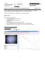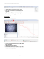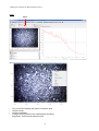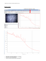
1
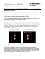
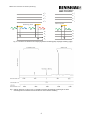
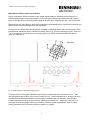
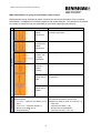
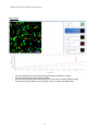
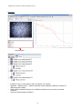
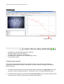
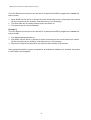
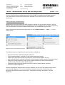
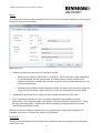
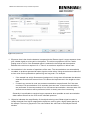
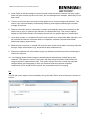
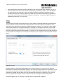
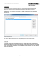
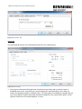
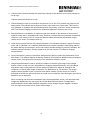
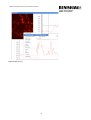
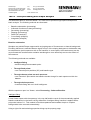
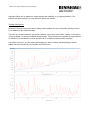
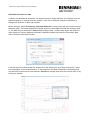
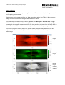
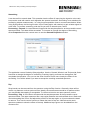
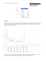
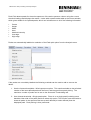
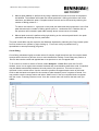
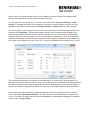
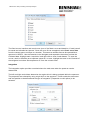
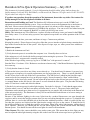
Renishaw InVia Quick Operation Summary—July 2015
This document is frequently updated—if you feel information should be added, please indicate that to the
facility manager (currently Prof. Kit Umbach, [email protected], Thurston 114, office and cell: 607-216-8872).
All procedures are subject to change.
If you have any questions about the operation of the instrument, do not take any risks—first contact the
facility manager: he has his cell phone with him at all times.
Reservations and Enabling on Coral: The Renishaw InVia Raman microscope is on the CCMR Coral
equipment reservation and enabling system. Users are allowed to reserve the instrument for as much time as
they need. However users who reserve time and do not cancel it in advance will be charged; abuse of the
reservation system can result in suspension of CCMR facility privileges. You can access Coral either from your
laptop or from the Coral computer in Bard B47, to which you will be given access.
Safety: This instrument uses Class IIIb lasers, so please be alert to the safety issues you learned in the EH&S
laser safety course. Use of laser safety eyewear is not required except in the case of the operation of the 532 nm
laser.
Logbook: Record the date, your name, and hours of usage. Comment on problems.
Keeping lab orderly: Please dispose of any glass slides that you use into the red plastic sharps container that is
kept on the floor near the base of the system. Also dispose of wipes, tape, etc. when you are done with them.
Steps to run system:
1) Enable the instrument on Coral.
2) Verify that main power is on and that the computer is on. Normally these are left on.
If the main power is off, check with facility manager before turning the system on. The computer can be
rebooted if needed—no password is currently needed.
If the Windows logon dialog comes up, log on as “CCMR-User” with password “ccmruser”.
Start the Wire 4.1 software. Pick “Reference un-referenced motors only” if the Motor Reference Options dialog
box comes up.
3) Verify that the shutter is closed.
4) Turn on the lasers you wish to use if they are not already on. You should wait 10 minutes if you need very
stable power or frequency; for a quick measurement you can begin right away. There is a switch (labeled L1)
for the 785 nm laser on the side of the InVia spectrometer. The 488 nm laser (which has the blue fiber optic
connected to the laser output) has a key on the power supply. It must be turned to “Start” and held there
momentarily for the laser to be started. Do not adjust the power knob on the 488 nm laser power supply! There
is a manual shutter on the 488, but it is left open so as not to disturb the fiber optics. The procedure for turning
on the 532 nm laser is at the end of this document.
5) Set the Leica microscope up for white light imaging. Put in the 5x objective. Verify that the upper mirror
selection wheel is set to 2 and the lower mirror selection wheel is set to 1. The power on the white light
illuminator can be turned up to whatever level is appropriate for you sample (this is the wheel at the bottom left
of the microscope body). The illuminator is always left on and should be turned down to its lowest setting at
the end of your session.
Because of the different lighting in the room, light from the overhead fluorescents can enter through the
eyepieces and be seen in the imaging camera when you are not looking through the eyepieces. To eliminate this
problem, there is a rod on the left hand side of the trinocular with three positions—when it is pulled all the way
out, then the eyepieces are blocked and the light from the sample only goes to the camera. It should be left in
the middle position for use of both the eyepieces and camera. When using white light imaging, pulling the rod
out is optional. However you should pull the rod out when aligning the system with the lasers and taking
Raman spectra. You should also turn off the room lights for sensitive measurements.
Video Camera: The video camera should be set to not have auto-gain. This means that in white light you may
need to adjust the white light intensity using the dial on the lower left of the microscope base to get the best
white light image. In normal operation, you should not need to change the settings for the microscope camera.
If for some reason you need to increase the gain on the camera (or if the computer has not opened the video
camera) follow the instructions below. If you do need to change the settings, then you MUST restore them to
their original settings before you end your session on the microscope. The original settings are on the desktop
in a file “Video_Settings.” Failure to restore to the original settings will result in a usage charge—repeated
failures could result in restrictions on your access to the Raman microscope.
If Wire software does not open the Video Camera: Under View, choose Live Video. If you cannot see the
sample well. then you can turn on AutoGain—right click when the mouse is in the field of view of the video
camera, then choose Video Properties, then VideoSource tab, then CaptureFilterProperties, then in the Image
Controls window, check on Full Auto. As mentioned above, please restore the video settings back to where
they were originally when you are through with your session.
6) Place the Si reference sample underneath the objective and focus on the Si using white light. Rotate in
increasingly higher power objectives until you have the 100x in place. You can use the regular 50x objective
but because of some absorption due to coatings on the objective, the signal strength with the 50x will be lower
than with the 100x, most noticeably with the 488 nm laser. If you are imaging powders, liquids, foils, or fibers,
you should use the 50x long working distance objective (which is a different objective from the regular 50x
objective) and requires a short training--do not use the 50x long working distance objective without first getting
this training from the facility manager.
Remember that rotating the coarse and fine focus knobs counterclockwise (towards the
user) moves the microscope stage down.
7) For Raman imaging, switch the upper mirror selection wheel to 1 and the lower mirror selection wheel to 2.
Pull out the camera selection rod on the upper left side of the microscope trinocular to the fully out position,
which ensures that no light gets to the eyepieces.
8) DO NOT LOOK THROUGH THE EYEPIECE FROM THIS POINT ONWARD—USE THE CCD
CAMERA IMAGE ON THE SOFTWARE!
9) The only manual adjustment of hardware you need to make in the spectrometer are the three lenses and the
pinhole—do not touch the filters! The lenses that need changing when you go to a different laser are the
A2,B2,C2 (for 488 and 532 nm) and A1,B1,C1 (for 785 nm) lenses. The pinhole should be in for 785 nm
operation and out for 488 and 532 nm operation.
The Rayleigh filters are on a motorized rotating panel and will be put in place automatically when you choose
the laser using the menus along the bottom of the main software panel (there is an icon that looks like a laser
spot), either “SM 488 nm Raman” for the 488 nm or “785 nm edge” for the 785 nm or “SM 532 nm ULF
Raman” for the ultra-low frequency Rayleigh filter operating with the 532 nm laser. If you want to use the 532
nm laser for high-speed, large area imaging, see the facility manager about manually replacing the 488 nm
Rayleigh filter with a 532 nm Rayleigh edge filter.
You also need to pick a grating in software. For 488 excitation, pick the 2400 l/mm grating using the pull down
menu at the bottom of the main software panel. For 785 excitation, pick the 1200 l/mm grating using the pull
down menu. For 532 nm ULF filter operation, choose the 2400 l/mm grating. For high-speed imaging with the
532 nm laser, you can use either the 2400 l/mm grating or manually replace that grating with a 600 l/mm
grating (see the facility manager for additional training on changing the filters manually, high-speed imaging
and using the ULF).
10) Open the shutter. If you get an error box “Warning: Interlock relays are disabled” check that the
spectrometer door is locked tight. Then hit “Retry” in the error box. At that point it is possible that the 785 nm
laser needs to be restarted if that is the laser you are using—close the shutter and open it again to restart the 785
nm laser.
11) Bring the power up to about 50% or 100%, make sure you have picked the SLOWEST speed on the
trackball control and use the fine focus ring on the microscope track ball to sharpen the image of the laser.
Adjust the fine focus ring in small steps or you risk crashing the objective into the sample.
12) Under the “Measurement” pull-down menu on the top menu bar, pick “New Spectral Acquisition”. Take a
static spectrum at the wavelength you want to use. At 785 nm that you should take the alignment spectrum at
100% power; at 100% you should see 10,000 counts for a 1 second acquisition time. At 100% power for 488
nm, counts are at 7,000 for a 1 second acquisition time.
If you are not getting these counts, you will need to first manually align the laser beam position to be at the
center of the crosshair box in the video image. This is done with the “Manual Beamsteer” option in the pulldown menu on the top menu bar under “Tools”.
When using Manual Beamsteer, Only use the left set of arrows when steering the beam manually.
After centering the beam, use AutoAlign (goto “Tools>AutoAlign>Align” ) for the CCD and the slits. Do no
use AutoAlign for the laser position—use it only for the CCD and slits after you have manually aligned the
laser position.
As indicated above, before using Manual Beamsteer, set up and run a measurement. Anytime you use Manual
Beamsteer, you should then do Align CCD Area followed by Auto Align Slit (Optimise).
Important Warning on AutoAlign CCD: the AutoAlign CCD will give you “Initial” and “Final” values of the
pixels on the CCD where the system will collect the Raman scattered light. These pixels should be in the range
from 15 to 30 for 488 nm and 1 to 15 for 785 nm. Sometimes the routine makes an error and gives as a final
value a range of pixels that is far from the initial. If this happens, do not accept the results—revert and just use
the initial values.
If after doing these things, the counts are less than 50% of the expected values, please make a note in the
logbook.
For the 785 nm laser, the spot is defined by a pinhole. The pinhole is manual and needs to be left in for 785 and
moved to the out position for 488 and 532 nm operation. For those of you who want more signal with 785 nm,
you can leave the pinhole out so that your sample is illuminated by the full beam profile of the laser, which is a
line—however you will lose spatial resolution and the facility manager will need to show you how adjust the
CCD area to take full advantage of this extra power.
13) From the Tools menu, pick “Calibration>Quick Calibration” to ensure that the spectral calibration of the
instrument is correct.
14) Rotate out 100x and place your sample onto the microscope stage. Proceed with your sample measurement.
More information on setting up measurements is available in the photocopied Renishaw documents and via the
Help files of the Wire software.
15) Shutdown: Put the 5x objective into place, lower the microscope stage, remove your sample, put the mirror
selection wheels into the position for White Light imaging, turn down the intensity of the micrsoscope halogen
illuminator with the dial at the lower left of the micrsoscope base, exit the Wire software, turn off whatever
laser you are using, exit Coral.
Operating Tips:
When you are setting up a new measurement and are in the “Acquisition” tab, there is an option “Restore
instrument state on completion.” Check this option. This will bring the power to whatever level you have set it
to manually after the measurement is done. You can also choose the option of closing the shutter after the
measurement to avoid overexposing light-sensitive samples.
The origin of the mapping stage can be reset to zero by picking “Choose Origin” under the “Live Video” pull
down menu along the top menu bar.
Be careful about making sure that confocality is set to “Standard” and not to “High” in the Range tab in the
Measurement Setup window.
We have changed the sign convention for the z-stage position: more negative now means deeper into sample
(same as moving stage up)
Turning the 532 nm laser on
Make sure the 532 nm laser cooling fan is turned on at the terminal strip (you should be able to hear the fan,
but do not reach in to check the fan at the laser because you may disturb the optics).
Put on laser safety goggles.
Start the laser software on computer; the software is called “Cobolt Monitor”
Pull down the File menu and choose “Connect”
Click on the radio button “Set Power”
Set laser power level in software to 40 mW.
Click on the “Restart” button in the software.
Turn on the power key to laser.
The message box on the right hand side of the Cobolt Monitor software window should quickly highlight in
blue the “Warming Up” message. If it is stuck on the “Waiting for Key” message, turn the key off, wait 20
seconds, hit “Restart” and turn the key back on.
Wait until the message box shows “Completed” highlighted in blue.
Remove safety goggles.
You can adjust the laser power with the software from that point on. If you adjust the power above 100 mW,
put the laser goggles on whenever the shutter is open.
Turning off 532 nm laser.
Turn the power key on the laser off.
Turn down the power in the software.
Disconnect the laser from the Cobolt software.
Wait 2 minutes and turn off the 532 nm laser cooling fan at the terminal strip.
Exit the laser software.
Installing Wire 4.1 on your computer
You can get Wire 4.1 from the desktop on the new computer—the folder is called “Wire 4.1 CD” (it is also
available to Cornell users as a zipped file at https://cornell.box.com/s/gxy4pkeo2od1bdukdx3d). Copy this
folder to your memory stick and follow the instructions in the file “Wire Install Notes” that is in the “Wire 4.1
CD” folder. Be especially careful to copy the “Wire 4.1 CD” to your desktop—do not try to install from the
memory stick directly. You do not need to uninstall Wire 3.4.
Help File
The user guide is on the desktop as “User Guide.chm” and is also available at
http://www.ccmr.cornell.edu/raman
Storing Data
ALL data should be stored on the Users folder on the D: drive in a folder with your netID as its name—there is
a shortcut on the desktop to this Users folder. I have transferred all user folders dating from 2013 and later from
the old User folder to the new User folder. If you need to get to your data or measurement settings from the old
computer, let me know.
No longer will any data files on the desktop or on the system drive be tolerated—they will be deleted. You
must put your data onto the Users folder on the D: drive.
Data Formats
Renishaw now uses a new data format (wdf) instead of wxd. This format cannot be read by Wire 3.4. However
all the data that you took with Wire 3.4 as wxd files can be read by Wire 4.1. So if you want to view the data
you take with Wire 4.1, you can either save your data as txt files, in which case you can use Wire 3.4 or Wire
4.1 or other programs to view the data, or you need to install Wire 4.1 on a Windows 7 machine to view the wdf
files. According to Renishaw, Wire 4.1 is not going to function with XP or with Windows 8 but some users
have been able to install Wire 4.1 on Windows 8 machines, so you can give it a try.
Raman Users,
Occasionally the Raman system has problems with very low counts on the Si or you are seeing
the laser as a line instead of a spot.
This might occur because of a system crash, after which a dialog box comes up and you are asked to
“re-reference the motors.” Then the optics might start out in a “bad” position where some of the light is
blocked as it passes toward the Rayleigh filter. So after re-reterencing, even if you don’t see a laser
beam on the sample, just run a measurement and the optics position should correct itself. If it looks
like the optics on the linefocus motor are staying in a "bad" position after you run a measurement
follow the procedure below.
1)
2)
3)
4)
From the Tools menu, choose “Reference Motors”
Choose “Reference selected motors” and highlight in the list to the left ONLY “Linefocus motor”
Click on “OK”
Go through the following process below for moving the optics to “Good”
To move the wheel to the GOOD position, first choose the laser “785 nm Linefocus” if you are
using 785 nm or “SM 488 nm Raman Linefocus” if you are using 488 nm. This will move the
wheel to close to the WORST position. Then choose the laser “Multi-Line Fiber Raman”. This
should rotate the wheel to the GOOD position. Open the spectrometer door and check the
wheel position. If it is not in the GOOD position, close the door, and choose the “Linefocus”
laser setting you used before , and then try again “Multi-Line Fiber Raman”. Repeat until the
wheel is in the GOOD position. Then pick the laser your normally use. If this repeatedly fails,
then start the entire process with the other linefocus laser setting than you started with.
!
!
!
GOOD
BAD
!
VERY BAD
WORST
Renishaw plc
Spectroscopy Products Division
Old Town, Wotton-under-Edge,
Gloucestershire GL12 7DW
United Kingdom
Tel
Fax
Email
+44 (0) 1453 524524
+44 (0) 1453 523901
[email protected]
www.renishaw.com
TM001 - Introduction to Raman spectroscopy
WiRE™ 4.0
What is Raman scattering?
Raman scattering is named after the Indian scientist C.V. Raman who discovered the effect in
1928. If light of a single colour (wavelength) is shone on a material, most scatters off with no
change in the colour of the light (Rayleigh scattered light). However a tiny fraction of the light
(normally about 1 part in 10 million) is scattered with a slightly different colour (Raman scattered).
This light changes colour because it exchanges energy with vibrations in the material. This makes
Raman scattering an excellent tool for probing vibrations in materials.
The aim of Raman spectroscopy is to analyse the Raman scattered light and infer from it as much
as possible about the chemistry and structure of the material.
More on Raman scattering
Scattering occurs when an electromagnetic wave encounters a molecule, or passes through a
lattice. When light encounters a molecule, the vast majority of photons (>99.999%) are elastically
scattered; this Rayleigh scattering has the same wavelength as the incident light. However, a small
proportion (<0.001%) will undergo inelastic (or Raman) scattering where the scattered light
undergoes a shift in energy; this shift is characteristic of the species present in the sample. This
process is shown in in Figure 1.
Before Raman scattering
After Raman scattering
Molecule vibrating
Molecule
Laser
excitation
Raman
scattering
Fig. 1. Schematic diagram of the Raman effect
Figure 2 illustrates the transitions accompanying Rayleigh and Raman scattering. The electric field
of the incident light distorts the molecule’s electron cloud, causing it to undergo electronic
transitions to a higher energy ‘virtual state’; not a true quantum mechanical state of the molecule.
Raman scattering results in the release of a scattered photon with different energy to the incident
photon; the difference in energy is equal to the vibrational transition, ΔE. The relative intensity of
stoeks ans anti-Stokes lines at room temperature is shown in Figure 3.
-1-
TM001-02-A Introduction to Raman spectroscopy
v’3
v’2
v’1
v’0
v’3
v’2
v’1
v’0
Virtual energy level
Virtual energy levels
hvi
hvs = hvi - ΔE
hvi
hvs = hvi + ΔE
ΔE
v3
v2
v1
v0
hvi
hvs = hvi
Fig. 2. The electronic transitions accompanying Raman scattering (left), Rayleigh scattering (right)
Fig. 3. Raman spectrum of silicon (514 nm excitation) showing the Rayleigh scattering at the laser
wavelength and the Stokes and anti-Stokes line of the Raman scattering
2
v3
v2
v1
v0
TM001-02-A Introduction to Raman spectroscopy
What does a Raman spectrum look like?
Figure 4 shows the Raman spectra of two carbon based species, diamond and polystyrene. In
Raman spectroscopy we are interested in how much the scattered light differs from the incident
light, so the spectrum is normally plotted against the difference between the two - the Raman shift.
Diamond has one main Raman band only because the tetrahedral lattice is symmetrical and all the
carbon atoms and connecting bonds are equivalent.
Polystyrene has different functional groups consisting of differing atoms and bond strengths. Each
Raman band represents either a discrete function group (e.g. C-H from benzyl group at ~3200 cm1
) or a combining of small groups into a larger group (e.g. C6H5R breathing mode from benzyl
group at ~1000 cm-1).
Diamond
Fig. 4. Raman spectra of diamond and polystyrene
The bottom axis of the graph represents the energy of the Raman shift (measured in cm-1) and
may be plotted right-to-left or vice versa. A value of 0 cm-1 would indicate that no energy has been
exchanged with the sample and the incident light is scattered with no change in wavenumber.
Carbon-hydrogen bonds give rise to Raman bands around 3000 cm-1, due to the small mass of
hydrogen and resulting high frequency vibrations. Peaks at lower wavenumber relate to lower
energy vibrations such as those of bonds to carbon or oxygen.
3
TM001-02-A Introduction to Raman spectroscopy
What information can you get from Raman spectroscopy?
Raman bands can be analysed to obtain chemical and structural information for the material
identification, investigation of material properties and spatial analysis. The table below illustrates
the variety of results that can be obtained from point and mapping measurements.
Band parameter
Univariate
Characteristic
Raman
frequencies
Information
Identification
(material composition)
Compare
characteristic
Raman
frequencies
Differentiation
Intensity
variation with
changing
polarisation
Crystallographic orientation
Variation in
absolute /
relative
intensity
Absolute / relative concentration
Variation in
Raman band
width
Crystallinity;
Temperature
Variation in
Raman band
position
Stress state
Multiple spectra
Any of the above parameters applied to
Any of the above information in conjunction
multiple spectra:
with different dimensions such as time,
• Univariate – based on raw data or curve temperature, distance, area, and volume, e.g.
fitting.
• Thickness
• Multivariate – algorithm based e.g.
(Intensity with depth – 1D)
DCLS, PCA, MCR-ALS or
• Domain size and distribution
TM
EmptyModelling .
(Intensity with area – 2D / 3D)
Table 1. Information obtainable from analysis of different Raman band parameters.
4
TM001-02-A Introduction to Raman spectroscopy
Raman spectroscopy obtains such information by probing the vibrational states of materials.
Renishaw’s inVia can also be used for photoluminescence (PL) measurements, which is a
competing effect to Raman. PL is typically much stronger in intensity and is a function of the
electronic states of the material. The PL effect can sometimes provide an unwanted broad
background that can mask the Raman bands. However, PL measurements can also provide useful
complementary information on material properties such as conjugation, structural vacancy, and
atomic substitutions.
What does a micro-Raman instrument usually consist of?
It usually consists of:
•
•
•
•
•
•
A monochromatic light source (normally a laser)
A means of shining the light on the sample and collecting the scattered light (often this is a
microscope)
A means of filtering out all the light except for the tiny fraction that has been Raman scattered
(often holographic ‘notch’ or dielectric ‘edge’ filters)
A device (such as a diffraction grating) for splitting the Raman scattered light into component
wavelengths, i.e. a spectrum.
A light-sensitive device for detecting this light (normally a CCD camera)
A computer to control the instrument and the motors and analyse and store the data
Figure 5 shows the layout of Renishaw’s inVia Reflex Raman microscope, with all the key
components highlighted.
Research grade Leica
microscope
Auto excitation
wavelength
switching
Auto
confocality
control
Ultra-high
precision multiple
grating stage
Auto view/Raman
changeover
Auto calibration
Auto performance
verification
UV capability
Raman imaging
capability
Near-excitation filter
capability
Wavelength
optimized
laser beam control
Class 1 laser safe
enclosure
Flexible sample
handling
Auto alignment
optimization
Safety interlock
control
Fig. 5. Renishaw’s inVia Reflex Raman microscope
5
Renishaw plc
Spectroscopy Products Division
Old Town, Wotton-under-Edge,
Gloucestershire GL12 7DW
United Kingdom
Tel
Fax
Email
+44 (0) 1453 524524
+44 (0) 1453 523901
[email protected]
www.renishaw.com
TM002 – Introduction to WiRE and System start-up
WiRE™ 4.0
The aim of this module is to provide a general overview of the WiRE software, and detail the
correct procedure for Raman microscope, laser, PC, and software start-up.
Please note that this module is a guide and not a complete protocol.
WiRE software
WiRE software is designed to:
• Control Renishaw Raman instruments
• View the sample
• Control data collection parameters
• View data
• Provide processing functions to improve data
• Provide analysis options to determine information from Raman data
• Enable data and results to be printed and exported for analysis / reporting
Architecture of the WiRE software
Menu and toolbar
Menu and toolbar
-1-
TM002-02-A Introduction to WiRE and System start-up
•
•
•
•
Toolbar buttons offer shortcuts to menu items
Right click on the toolbar to control which groups
are shown.
Right click on a group to control the individual
buttons which are shown
The toolbar contents is configurable for different
users who log on to the PC
Sample review
Sample review
•
•
•
•
Controls the view of the sample on the video (white
light, and/or laser)
Aids focussing onto the sample
Opens/closes the instrument shutter for laser entry
into the instrument
Controls the laser – grating – detector configuration
used for new measurements
2
TM002-02-A Introduction to WiRE and System start-up
Video
Video
•
•
•
•
Turn on/off and change the type of crosshair used
View the axes
View the scalebat
Change the properties fo the video display including
brightness, contrast and exposure time
3
TM002-02-A Introduction to WiRE and System start-up
Spectrum viewer
Window with spectrum viewer
•
•
•
View and control the spectrum, or spectra
Control the view (add labels)
4
View processing and analysis operations
TM002-02-A Introduction to WiRE and System start-up
Map review
•
•
•
•
View the individual or combined white light image and Raman images
View spectra from different image locations
Review how spectra have been analysed in conjunction with the Raman image
Access the look up table to control image colour, contrast and brightness
5
TM002-02-A Introduction to WiRE and System start-up
Navigator
The Navigator
•
•
•
•
•
•
Enables control of what data is open and where it is viewed
Windows – Measurement - Viewers and data housed together (different viewers for
different types of data)
Measurement enables identical (or modified) conditions to be used for new data
collection
Access to experimental conditions
Control of spectra from multi-files
Saving of spectra, profiles and images
6
TM002-02-A Introduction to WiRE and System start-up
Notification area
Notification area
• Progress bar indicating data acquisition progress
• File signing when using 21 CFR pt 11
• Sample location within video (XYZ values)
• XY spectrum co-ordinates or XYi Raman image values
• Laser interlock status
• Instrument active indicators
• Access to experimental conditions
• Controlsystem
of spectra
from multi-files
Complete
start-up
• Saving of spectra, profiles and images
This procedure assumes all electrical components relating to the use of the inVia Raman
microscope are switched off initially, and that the user has suitable knowledge of Renishaw’s
WiRE 4 software.
1. Turn on the system using the main on/off power button situated to the right hand side of the
instrument. (the CCD camera will take ~ 20 minutes to cool to its operating temperature).
2. Turn on the desired laser(s), and ensure all keys and switches are correctly set (please refer
to the laser user manual for individual laser start-up procedures)
7
TM002-02-A Introduction to WiRE and System start-up
3. The laser interlocks will not be activated until the WiRE 4 software has been opened. From
point of lasing each laser requires at least 30 minutes to reach optimal pointing and power
stability.
4. Turn on the PC, and run the WiRE 4 programme.
5. The software will prompt for a position check of the relevant motors.
6. Choose the ‘Reference un-referenced motors only’ option, and click on ‘OK’.
Partial system start-up
Typically some of the components will already be on when the system is to be used, and therefore
the start-up procedure should be modified accordingly.
The following is an example of how the system might usually be found, and the correct procedure,
in this case, to complete the initial start-up.
Example 1
The inVia Raman microscope is on, and the PC is on and the WiRE 4 programme is open. All
lasers are off.
1. Clear all data and windows from WiRE 4 (checking that no unsaved data is further required).
2. Turn on the appropriate laser(s).
3. Wait for the required time period for the optimum laser stability to be reached.
Example 2
8
TM002-02-A Introduction to WiRE and System start-up
The inVia Raman microscope is on, and the PC is on and the WiRE 4 programme is closed. All
lasers are on.
1. Open WiRE 4 (there will be no prompt for motor referencing as the current state of the motors
will be recognised by the software, and referencing is not necessary).
2. The laser state will not change and all lasers will remain on.
3. The system can be used immediately.
Example 3
The inVia Raman microscope is on, and the PC is on and the WiRE 4 programme is closed. All
lasers are off.
1. Turn on the appropriate laser(s).
2. Run WiRE 4 (there will be no prompt for motor referencing as the current state of the motors
will be recognised by the software, and referencing is not necessary).
3. Wait for the required time period for the optimum laser stability to be reached.
Having powered up all the system components, and waited for stability to be reached, the system
is now ready to be configured.
9
Renishaw plc
Spectroscopy Products Division
Old Town, Wotton-under-Edge,
Gloucestershire GL12 7DW
United Kingdom
Tel
Fax
Email
+44 (0) 1453 524524
+44 (0) 1453 523901
[email protected]
www.renishaw.com
TM004 – Measurement set-up and data acquistion
WiRE™ 4.0
The aim of this module is to detail the correct use of WiRE 4 to enable spectral data collection
using the different measurement parameters available in conjunction with the inVia Raman
microscope.
Defining the type of measurement
Measurements are used within the WiRE software to define the type of data collection. Several
different types of measurement may be available to the user, depending on the exact configuration
of the inVia Raman microscope. Measurements which are unavailable are greyed out.
New measurements are accessed using either the menu (Measurement……New……), or the
toolbar arrow.
Figure 1 Toolbar new measurement access
Figure 2 Menu new measurement access
The different types of measurements which may be available are:
•
•
•
•
•
•
•
Spectral acquisition (standard spectral collection)
Filter image acquisition (collection of filter spectra and filter images)
Depth series acquisition (spectral collection at varying sample depths, Z only)
Map image acquisition (spectral collection at varying lateral sample positions and depth slices)
StreamLine image acquisition (high speed spectral collection at varying lateral sample
positions with a minimised laser power density)
StreamLineHR (high speed spectral collection at varying lateral sample positions)
StreamLineHR 3D acquisition
When the appropriate measurement has been selected, the set-up of that measurement will be
automatically displayed. This module details the standard set-up tabs, consistently used
throughout the different measurement types. These tabs are Range, Acquisition, File and
Advanced.
-1-
TM004-02-A Measurement set-up and data acquisition
Range
The Range tab covers the basic settings for the scan such as the laser and grating to be used, and
the type of scan to be performed.
Figure 3 Range tab
1. Grating scan type gives the option for two types of scan.
•
Static covers a range of about 200 cm-1 to 500 cm-1 either side of the centre, depending
on the wavelength and the grating used. The desired centre can be entered in the
Spectrum range box. A static scan is quicker to perform than an extended scan, but only
covers a limited range.
•
Extended (SynchroScan) scans between the upper and lower limits entered in Spectrum
range, and is used when a static scan will not cover the required wavenumber range.
2. Configuration allows the user to select the laser, grating and detector to be used.
3. The Confocality box allows the user to choose between high and standard confocal
performance. The confocality defines the sample volume that signal is collected from. Using
the High confocality option reduces this volume increasing the spatial resolution but also
reducing the total Raman signal
Note the instrument is always confocal due to the optical layout. High confocal mode is not
available in line focus or StreamLine imaging configurations.
Acquisition
The Acquisition tab allows the user to alter scan conditions such as the exposure time and laser
power to be used.
2
TM004-02-A Measurement set-up and data acquisition
Figure 4 Acquisition tab
1. Exposure time is the time the detector is exposed to the Raman signal. Longer exposure times
give a better signal-to-noise ratio in the spectra. The minimum exposure time for a static
grating scan is 0.02 s. If the Extended option is selected in the Range tab the exposure
defaults to the minimum required: 10 s. There is no maximum exposure in either case.
2. Accumulations is the number of repetitions of the scan. The accumulations are automatically
co-added, to produce spectra with better signal-to-noise ratios. Using several accumulations of
a short scan can be preferable to performing one long scan. For example:
•
•
If the sample has a high fluorescence background, a long scan will saturate the detector,
whereas several short scans will not. This allows an improvement in the single-to-noise
ratio.
If cosmic ray removal is used, two extra accumulations are performed. So if the scan
consists of 10 accumulations of 10 seconds, then two extra 10 second accumulations
are performed. If the scan consists of one 100 second accumulation, then two extra 100
second accumulations will be performed, which is clearly more time consuming.
Generally it is preferable to conduct longer exposures when possible as each accumulation
adds readout noise from the CCD to the collected spectrum.
3. Objective indicates the magnification of the objective being used. Better signal-to-noise is
usually obtained from higher magnification objectives, as they give a higher power density at
the sample. The box is greyed-out. The value reflects the value set in the Sample Review
window.
3
TM004-02-A Measurement set-up and data acquisition
4. Laser Power is the percentage of maximum laser power that will be used for the scan. Higher
power will give a better signal-to noise ratio, but can damage some samples, depending on the
laser used.
5. Cosmic ray removal removes random sharp peaks due to cosmic background radiation. The
cosmic rays are eliminated by automatically obtaining three spectra and taking the median
average of the three.
6. Restore instrument state on completion is used to automatically restore the instrument to the
state it was in prior to collection (as defined in the Sample Review). This function applies
largely to inVia Reflex Raman microscopes where there is a greater degree of motorisation.
7. Close laser shutter on completion forces the laser shutter to be closed after data collection, and
will override the Restore instrument state on completion checkbox (recommended when
performing imaging experiments).
8. Minimise laser exposure on sample will close the laser shutter when data is not being collected
during a single measurement (e.g. temperature ramp measurement)
9. Response calibration will collect data using a pre-defined transmission profile normalising the
instrument response.
10. Live imaging allows Raman images to be defined and subsequently viewed during data
collection. This feature is used in conjunction with Map image acquisition and StreamLine
image acquisition measurements only. This option requires the user to know the expected
changes within the Raman data or have pre-collected reference spectra of specific
components. (PCA and MCR-ALS options are not possible with Live imaging).
File
The File tab covers options for automatically saving the data. Either insert a filename or browse to
a folder.
Figure 5 File tab
4
TM004-02-A Measurement set-up and data acquisition
1. Autosave file saves the file to the file specified in File name directly after collection. Its use is
recommended, as it removes the risk of losing data by forgetting to save it. The next dataset
will overwrite the first unless the Auto increment checkbox is selected. Checking the Auto
increment function will force the data to be saved each time this measurement is performed.
The format will be filename, filename0, filename1, filename2…unless the original filename is
appended numerically, e.g. filename1.
Timing
The Timing tab consists of two main functions: time series and sample bleaching measurements.
The Time series measurement allows multiple spectra, with same instrument conditions, to be
acquired with an identical period of time elapsing between each one. This function may be useful
to monitor the lifetime of a biological sample, for example, by its Raman spectrum. Set the total
number of spectra to be acquired in the first box ('Number of acquisitions') and the interval in the
second ('Time series measurement settings'). A ‘profile’ can be created at the end of the sequence
from the data. For example, the intensity at one frequency in the spectrum with acquisition number
(time).
Figure 6 Timing tab
Sample bleaching, also called photobleaching or photoquenching, is a phenomenon whereby
fluorescence is observed to decrease simply by the having the laser incident on the sample. There
are various mechanisms that part contribute all or in part to this effect. Setting a value in the box
exposes the sample with the laser for a set time before the spectrum is acquired. The period of
time may range from seconds to tens of minutes and will be sample and laser dependent.
Software triggering is only required in special cases using external hardware.
5
TM004-02-A Measurement set-up and data acquisition
Temperature
The temperature series measurement tab is only available when suitable heating/freezing
temperature stages have been installed with the appropriate WiRE feature permission.
By default, the ‘use’ check box is unchecked. To activate the temperature series parameters,
check the box.
Figure 7 Temperature tab
See module TM22 for instructions on the set up of temperature series measurements.
FocusTrack
To maintain the laser focus for spectral acquisition, for example, during time, temperature and
mapping measurements, you may use the FocusTrack function. Refer to module TM6 for guidance
notes. The 'Focustrack' tab allows the user to enable this function and specify how often it is used
during the measurement.
6
TM004-02-A Measurement set-up and data acquisition
Figure 8 FocusTrack tab
Advanced
The advanced tab covers more specialised options for the measurement.
Figure 9 Advanced tab
1. Scan type is used when Extended scan is selected in the Range tab to select the type of
extended scan to use. SynchroScan is recommended for most applications, as it does not
contain the artefacts present in stitched scans. The Step option is included for samples that are
very strong Raman scatters and might saturate the detector if the SynchroScan option, which
requires a minimum 10 second exposure, is used.
7
TM004-02-A Measurement set-up and data acquisition
2. Camera Gain switches between the sensitivity settings of the detector, and should usually be
set to high.
Camera Speed should be set to low
3. Pinhole allows the user to set whether the pinhole is In or Out. The pinhole may improve the
beam profile. The pinhole can be used to convert a line laser into a spot laser. This function
only operates on systems with a motorised pinhole. Its primary uses are in those instruments
with True Raman imaging and where the automated alignment functions are set up.
4. Binning allows the co-addition of adjacent signal from pixels on the detector to improve the
signal-to-noise ratio in extended scans only. However, excessive binning reduces the spectral
resolution. Use values of 2 or 3 unless the Raman bands are naturally broad when larger
values can be used. The default value is 1.
5. Laser focus controls the use of the beam expander. 0% indicates the laser is tightly focussed,
while 100 % indicates it is completely defocused by the beam expander. Defocusing reduces
the power density at the sample, and so can reduce sample damage in sensitive samples, but
reduces spectral resolution. Values greater than 0% are used for True Raman imaging
measurements.
6. Input polarisation is used in instruments with polarising filters to select the polarisation of the
laser beam. The different Raman scattering response of a sample to different laser polarisation
can be useful in assigning the symmetry of the vibrational modes involved.
7. Image capture allows the user to specify the capture of a white light image of the sample
before or after, or both for time, temperature or mapping measurements by using the Mode
drop-down menu. Delay sets the time the camera is allowed to adjust its settings to the
conditions, so that a good image is obtained. The default time is 2.5 seconds. The image
capture feature applies to both inVia and inVia Reflex models. On the former, the user is
prompted to switch the optics such that an image can be collected, then back again such that a
spectrum can be acquired.
When reviewing one-dimensional datasets (time and temperature series), the acquired video
images are displayed in the top right frame of the Map Review window. If images were
acquired (before and/or after) spectral acquisition, these images may be toggled / selected
from the right-click context menu (Show video image…).
8
TM004-02-A Measurement set-up and data acquisition
Figure 10 Map Review
9
Renishaw plc
Spectroscopy Products Division
Old Town, Wotton-under-Edge,
Gloucestershire GL12 7DW
United Kingdom
Tel
Fax
Email
+44 (0) 1453 524524
+44 (0) 1453 523901
[email protected]
www.renishaw.com
TM012 - Data processing and simple analysis
WiRE™ 4.0
This document aims to show the WiRE™ 4.0 user how to process single spectra and perform
basic analysis. The following methods are discussed:
•
•
•
•
•
•
•
Baseline subtraction (processing)
Arithmetic functions on data (processing)
Smoothing (processing)
Zapping (processing)
Peak Pick (analysis)
Curve-fitting (analysis)
Integration (analysis)
Baseline subtraction
Samples may exhibit Raman spectra with varying degrees of fluorescence or thermal background.
Providing that there is sufficient Raman signal ‘on top’ of the sloping background, the baseline may
be subtracted to yield a spectrum with a ‘flat’ baseline. In some cases, the measurement can be
re-performed with an alternative excitation wavelength to more effectively remove the effects of
fluorescence.
The following methods are available:
•
Intelligent fitting
– default intelligent automated option
•
Through fixed points
– user controls point positions (XY) and baseline type
•
Through chosen points on each spectrum
– user controls X point which the baseline travels through for each spectrum within the
dataset
•
Through whole spectrum
– Automatic fitting with no in-built intelligence
With the spectrum open in a Viewer, select Processing…Subtract Baseline.
Intelligent fitting
A new Viewer opens with the spectrum in the top half and the result of the automatically applied
baseline subtraction in the lower half. By default the ‘Intelligent fitting’ baseline is applied with a
polynomial value of 11. This method is Renishaw patented and enables simple or complex
backgrounds to be removed automatically.
Using a right click and selecting properties brings up the property page:
TM012-02-A Data processing and simple analysis
Here the polynomial order can be adjusted if a better fit is needed. The context menu also enables
exclude regions to be added to the spectrum. Excluded regions do not contribute to the fitting of
the baseline.
TM012-02-A Data processing and simple analysis
Intelligent fitting can be applied to single spectra and multifiles (e.g. mapping dataset). The
baseline will automatically ‘fit’ each spectrum within the multifile.
Through fixed points
Selecting ‘Through fixed points’ as the fitting mode enables the user to manually specify points in
XY to determine the baseline shape.
The user can choose between ‘polynomial’ (and the order) and ‘cubic spline’ options. Cubic spline
is only available if 2 points are added (4 total points). This method can be applied to single spectra
or multifiles, but the baseline is fixed and will not ‘fit’ to different spectra within multifiles.
It is useful to zoom in, by left-clicking and dragging in either window, and adjusting the points
added in the top window by moving them with the mouse.
TM012-02-A Data processing and simple analysis
Through chosen points on each spectrum
Selecting ‘Through chosen points on each spectrum’ as the fitting mode enables the user to
manually add points (vertical lines) to the spectrum which are fixed to the data.
The user can choose between ‘polynomial’ (and the order) and ‘cubic spline’ options. Cubic spline
is only available if 2 points are added (4 total points).
This method can be applied to single spectra or multifiles. When applying to a multifile, common X
positions where no Raman bands are present should be found. The baseline will optimise based
on the X position for each spectrum within the dataset.
TM012-02-A Data processing and simple analysis
Through whole spectrum
Selecting ‘Through whole spectrum’ automatically fits a defined polynomial order through the entire
spectrum.
The context menu enables exclude regions to be added to the spectrum. Excluded regions do not
contribute to the fitting of the baseline.
This method can be applied to single spectra or multifiles, and is a less intelligent equivalent to the
recommended intelligent fitting option.
Accepting a correction
When you are satisfied with the correction, either select Accept from the context menu or close
the window, upon which, there will be a prompt asking if you want to keep the correction.
To save the change to your file use the File…Save or Save as option from WiRE.
TM012-02-A Data processing and simple analysis
Arithmetic functions on data
A variety of mathematical operations can be performed on single data files. For example, you can
add files together or subtract one from another. It can be an effective method of subtracting a
background spectrum or filter ripple profile.
With a file open, select Processing…Spectral Arithmetic. A new viewer will open, split into three
separate areas. The upper displays the sample spectrum, the middle will show the ‘auxiliary’ data,
i.e. the data file you would like to add/subtract/multiply by/etc., and the lower region will show the
result spectrum. Use the Spectral Arithmetic Properties window to browse for the auxiliary data
and to select the arithmetic function.
It can be useful to multiply either the sample file or the auxiliary file by a factor so that the Y axes
are comparable. In the example below, 1* the sample file has been used and 2* the background
correction file used to remove the baseline. Accept the change either from the context menu or by
closing the window.
TM012-02-A Data processing and simple analysis
Image arithmetic
A special case of arithmetic is performing functions on Raman image data, i.e. images created
from mapping measurements.
Ratio images can be generated form the ‘Map generation’ option (see TM014). More complex
image arithmetic is performed using the data arithmetic option.
The initial image is loaded into the viewer (data tab of the Navigator...derived data…..right
click….. load dataset). Under Processing…Data arithmetic, select auxiliary data (image) by
browsing for the mapping measurement wxd file, then selecting the image from the drop down in
‘Use derived data’. Use the value boxes to adjust the Data and Auxiliary scaling.
The format (image or surface) and LUTs of each image (initial, auxiliary and result) can be
adjusted from the context menu (View…View mode and…LUT control). Accept or reject the
result image.
Image 1
Auxiliary
image
Result
image
(Image 1
divided by
auxillary)
TM012-02-A Data processing and simple analysis
Smoothing
It can be useful to smooth data. This operation has the effect of improving the signal to noise ratio
but must be used with caution as it degrades the spectral resolution. Smoothing is no substitute for
performing a better measurement, i.e. using longer acquisition times or more accumulations. When
using SynchroScan, the binning function can be used (again, with caution) to gain a better signal to
noise ratio. To perform smoothing, with the file you wish to smooth open, select
Processing…Smooth. A new window will open with the sample spectrum at the top and the result
spectrum below. This data will be smoothed. To increase or change the degree of smoothing,
select Properties from the context menu to see the Smooth Properties window.
The application uses a Savitsky-Golay algorithm. Use the ‘Smooth Window’ and ‘Polynomial Order’
functions to change the degree of smoothing. Pressing ‘Apply’ performs the change and ‘OK’
completes the operation. You can use the zoom function to see more closely the effect of the
smoothing. You will be asked if you want to accept the resulting smoothed spectrum.
Zap
Stray bands can be removed from the spectrum using the Zap function. Generally, these will be
cosmic ray features or other spurious lines. Ideally, the measurement would be re-performed but
you may decide that zapping is acceptable. To remove a band on an open spectrum, select
Processing…Zap. A new viewer will open with the sample spectrum at the top and the result
spectrum below. The upper spectrum has a zap region between two vertical black lines. Grab each
vertical bounding line in turn and adjust the position of the zap region so it just encloses the band
to remove. Then use the zoom function to isolate the band to zap out. Notice that the result
spectrum updates to show the effect of the zap. Additional zap regions can be added from the
context menu.
TM012-02-A Data processing and simple analysis
Peak Pick
Peak pick is a quick and simple method to label band positions on a spectrum and enable these to
be printed out together. To initiate peak picking select Analysis > Peak pick, or click the Peak pick
button on the Analysis toolbar.
Note that it may be necessary to maximise the window containing the active spectrum in order to
see the peak results table window, depending on where it is currently docked.
TM012-02-A Data processing and simple analysis
Peak Pick detects peaks for the active spectrum of the active spectrum viewer using the current
threshold settings and displays the results. It also adds a peak results table to the current window,
which gives details for the picked peaks, which can include some or all of the following information.
•
•
•
•
•
•
•
Centre
Height
Width
Area
Absolute intensity
Low edge
High edge
Peaks are automatically labelled on selection of the Peak pick option from the Analysis menu.
If the peaks are not suitably labelled the following methods can be used to add or remove the
labels:
1. Use the Autoset thresholds > Whole spectrum option. This sets thresholds so that a limited
number of the best-defined peaks will be found, and then performs peak picking. The
maximum number of peaks can be set on the Automatic Thresholding tab.
2. Use Autoset thresholds > Single peak option. Zoom-in on a single peak (including some
baseline either side of the peak) and then select this option. This function sets thresholds to
locate all peaks in the spectrum that are as well defined (or better defined) than the
displayed peak. Peak picking is then performed.
TM012-02-A Data processing and simple analysis
3. Manual peak addition is performed by using a double left mouse click close to the peak to
be labelled. The software will locate the closest peak with 3 falling point either side of the
maximum and label this peak. Complete manual control can be achieved by reducing the
number of falling points to 1.
To reduce this value to 1, right click on the peak pick table and select properties. In the find
peak tab reduce the number of falling points option to 1 and select OK. A double click on
the spectrum will now add a peak label exactly where mouse cursor is located.
4. Manual peak removal is performed by right clicking on the relevant peak label in the peak
pick table and selecting remove peak label
The peak result table may be copied to the Windows clipboard by selecting the Copy results option
from its context menu (shown by right-clicking it). From here it may be pasted into e.g.
spreadsheet or word-processing programs.
Curve-fitting
Curve-fitting calculates highly accurate values for simple, single bands but also for complex band
systems where there may be two, three or more bands that overlap. Curve-fitting can produce a
.wxc file that can be saved and applied later to a spectrum or set of mapped data.
To fit a curve to a band or series of bands, select Analysis…Curve fit to open the Curve fit
window, zoom in to a region that contains the band and some baseline data either side. A baseline
may be added automatically between the end points of the spectrum. This can be used, or
removed via the context menu. Use the mouse to position the approximate centre of the band.
Click to add the band and repeat for the centres of other bands if part of a system of bands. You
may need to use the context menu and select ‘Add Curves’ if the curve symbol does not appear
with the cursor. Pressing ‘Remove curve’ from the context menu will remove the last node you
added.
TM012-02-A Data processing and simple analysis
Select ‘Start Fit’ from the context menu to fit the added curves to the data. The algorithm will
perform many iterations until the best fit has been achieved.
You can save the curve fit file as a *.wxc from the context menu (Curve parameters….Save
curves). To reapply this saved curve ‘template’, perhaps to a similar sample, start the curve fit
application and use the context menu (Curve parameters…Load curves) and then ‘Start fit’.
You can modify or make changes to the curve fit using the Curve Fit Properties window from the
context menu Properties. This provides greater control over the fitting process instead of the
automatic parameters that are usually used. For example, you can choose to fix a band centre
instead of letting it ‘float’ during the curve fit, or apply limits to parameters. This can be useful for
complex band shapes. Curves can also be named, different types of baseline can be used or the
curve type can be defined. Use the ‘Curve Fit’, ‘Curves’ and ‘Baseline’ tabs to adjust the curve fit.
The context menu allows the truncation of the fitted region on zooming (Fit viewed region). It is
generally beneficial to have this ticked. If this is not active then the baseline form and height will be
somewhat dependent upon other bands that are present throughout the whole spectral range. It
may be necessary to re-apply the baseline on zooming, as its original position will be persisted.
A curve-fitting procedure produces a table of data; the columns are selected from the context
menu of the table (Show/hide columns). The table lists the various parameters for each of the
curves. The data in the table can be copied and pasted into a spreadsheet package, for example
(context menu, Copy results).
TM012-02-A Data processing and simple analysis
The fitted curves, baseline and result curve (sum of the fitted curves and baseline, if used) can all
be saved and reloaded as ‘spectra’. Once the curve fit has completed, select Save curve data
from the context menu and save to a location. This saves a multifile that can be opened like a
spectrum in WiRE 3. Use the Data tab in the Navigator and expand the branches to show the
Collected data. Highlight each ‘acquisition’ and right click to show ‘Load dataset’. To save the
curves, result, or baseline as a separate ‘spectrum’ or trace, highlight the trace in the View tab of
the navigator and select ‘Save spectrum as’ from the context menu.
Integration
The integration option provides a method where the total area under the spectrum can be
determined.
The left and right vertical bars determine the region which is being analysed within the spectrum.
The properties are selected by using a right click on the spectrum. These enable the exact start
and end position to be defined and the type of integration (Trapezoid or cubic spline) to be
selected.
TM012-02-A Data processing and simple analysis
Trapezoid calculates the area between adjacent points using a trapezium drawn between the
points and the x-axis.
Cubic spline approximates the spectrum with local cubic polynomial models and uses integration to
get an estimate for the area between adjacent points.
In each case the result is the sum of areas across all pairs of points in the region