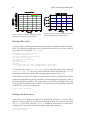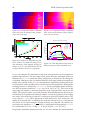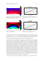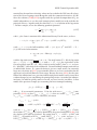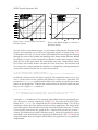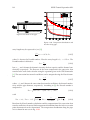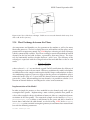
1
NM-SESES Multiphysics Software for Computer Aided Engineering Tutorial Version September 2012 Written by: J. Borth T. Graf T. Hocker E. Lang B. Neuenschwander B. Ruhstaller G. Sartoris H. Schwarzenbach NM Numerical Modelling GmbH Böhnirainstrasse 12 CH-8800 Thalwil Switzerland http://www.nmtec.ch mail://[email protected] Copyright, 1996 by NM Numerical Modelling GmbH. This work is subject to copyright. All rights are reserved, whether the whole or part of the material is concerned, specifically the rights of reprinting, reuse of illustrations, translation, broadcasting, reproduction or storage in data banks. Duplication of this publication or parts thereof is permitted in connection with reviews, personal or scholarly usage. Permission for use must be obtained, in writing, from NM . NM reserves the right to make changes in specifications at any time without notice. The information furnished by NM in this publication is believed to be accurate, however no responsibility is assumed for its use, nor for any infringement of patents or other rights of third parties resulting from its use. No license is granted under any patents, trademarks or other rights of NM . The author, NM Numerical Modelling GmbH, makes no representations, express or implied, with respect to this documentation or the software it describes, including without limitations, any implied warranties of merchantability or fitness for a particular purpose, all of which are expressly disclaimed. The author NM , its licensees, distributors and dealers shall in no event be liable for any indirect, incidental or consequential damages. NM wishes to record its gratitude to the numerous individuals that contributed, either through discussions, proposals, support or testing, to the development of this project. In particular, we wish to thank Prof. Dr. Edoardo Anderheggen who has over many years supported the design and development of SESES. The following institutions supported the authors during the initial development of SESES: Swiss Federal Institute of Technology in Zürich, the Commission for Technology and Innovation of the Swiss Federal Government and Landis & Gyr Zug. Contents Introduction 5 1 Getting Started 8 1.1 The SESES Environment . . . . . . . . . . . . . . . . . . . . . . . . . . . . 1.2 Building Your First Model . . . . . . . . . . . . . . . . . . . . . . . . . . . 12 1.3 Graphical Visualization . . . . . . . . . . . . . . . . . . . . . . . . . . . . . 15 1.4 Animation . . . . . . . . . . . . . . . . . . . . . . . . . . . . . . . . . . . . 16 1.5 Preprocess Mesh Definition . . . . . . . . . . . . . . . . . . . . . . . . . . 17 1.6 Algebraic Mesh Definition . . . . . . . . . . . . . . . . . . . . . . . . . . . 19 1.7 Non-Linear Algorithms . . . . . . . . . . . . . . . . . . . . . . . . . . . . 26 1.8 Continuation Methods . . . . . . . . . . . . . . . . . . . . . . . . . . . . . 31 1.9 External Post Processing and Controlling . . . . . . . . . . . . . . . . . . 34 2 Application Examples 8 38 2.1 Thermal strain . . . . . . . . . . . . . . . . . . . . . . . . . . . . . . . . . . 38 2.2 Designing a Hall Sensor . . . . . . . . . . . . . . . . . . . . . . . . . . . . 39 2.3 Electrothermally Driven Cantilever Microactuator . . . . . . . . . . . . . 43 2.4 Heat Conduction in a Cylindrical Stick . . . . . . . . . . . . . . . . . . . . 45 2.5 Image Acquisition in Scanning Probe Microscopy . . . . . . . . . . . . . 52 2.6 Cross Talk and Telegraphy . . . . . . . . . . . . . . . . . . . . . . . . . . . 55 2.7 Variable Gap Sensor . . . . . . . . . . . . . . . . . . . . . . . . . . . . . . 57 2.8 Modeling of a micro-reed switch . . . . . . . . . . . . . . . . . . . . . . . 60 2.9 Skin and Proximity Effect . . . . . . . . . . . . . . . . . . . . . . . . . . . 66 2.10 Steel Hardening . . . . . . . . . . . . . . . . . . . . . . . . . . . . . . . . . 71 2.11 Eddy Current Repulsion . . . . . . . . . . . . . . . . . . . . . . . . . . . . 74 3 4 SESES Tutorial September 2012 2.12 The total and reduced formulation of magnetostatic . . . . . . . . . . . . 77 2.13 The scalar and vector formulation of magnetostatic . . . . . . . . . . . . 81 2.14 Eddy currents in a linear system . . . . . . . . . . . . . . . . . . . . . . . 88 2.15 Preconditioning eddy current systems . . . . . . . . . . . . . . . . . . . . 97 2.16 Harmonic Analysis of a Piezoelectric Crystal . . . . . . . . . . . . . . . . 104 2.17 Longitudinally Diode Pumped Composite Laser Rod . . . . . . . . . . . 110 2.18 Thin-Disk Laser . . . . . . . . . . . . . . . . . . . . . . . . . . . . . . . . . 118 2.19 Thermo Optically Self-Compensated Amplifier . . . . . . . . . . . . . . . 126 2.20 Shells or Thin mechanical structures . . . . . . . . . . . . . . . . . . . . . 131 2.21 Plasticity Models . . . . . . . . . . . . . . . . . . . . . . . . . . . . . . . . 136 2.22 Necking of a circular bar . . . . . . . . . . . . . . . . . . . . . . . . . . . . 141 2.23 Stamping and mechanical contacts . . . . . . . . . . . . . . . . . . . . . . 149 2.24 Continuous casting of steel . . . . . . . . . . . . . . . . . . . . . . . . . . 157 2.25 Hagen-Poiseuille Model of Viscous Laminar Flow . . . . . . . . . . . . . 163 2.26 Blasius Plate Flow At Zero Incidence . . . . . . . . . . . . . . . . . . . . . 165 2.27 Microfluidic Mixing in a Straight Channel . . . . . . . . . . . . . . . . . . 168 2.28 Heat Transfer and Natural Convection in a Closed Cavity . . . . . . . . . 174 2.29 Calorimetric Flow Sensor . . . . . . . . . . . . . . . . . . . . . . . . . . . 180 2.30 Flow Around a Circular Cylinder . . . . . . . . . . . . . . . . . . . . . . . 186 2.31 Developing pipe flow with heat transfer . . . . . . . . . . . . . . . . . . . 191 2.32 Hot Spots in a Tubular Reactor . . . . . . . . . . . . . . . . . . . . . . . . 195 2.33 Effective Transport Parameters from Volume Averaging . . . . . . . . . . 200 2.34 Heat Exchange between Air Flows . . . . . . . . . . . . . . . . . . . . . . 204 2.35 A first model of a SOFC fuel cell . . . . . . . . . . . . . . . . . . . . . . . 206 2.36 A planar 2D+1D SOFC model . . . . . . . . . . . . . . . . . . . . . . . . . 210 Introduction Computer Aided Engineering (CAE) focuses on the application of physical-mathematical-numerical models to solve real-world multiphysics engineering problems. The past decade has been a period of rapid progress for CAE. The area of possible applications has been expanded and numerical methods have become increasingly sophisticated and adapted to exploit the available computational power of modern microprocessors. In particular, nowadays CAE-methods play a key role in the industrial product development process and help to • Speed-up the development cycle of products. • Optimize the product performance. • Develop a thorough understanding of the underlying physical-chemical processes. • Visualize device functionality not accessible through experiments. • Support the decision making process at different product development stages. • Eliminate potential failures and identify pitfalls. In general, the design of a physical-mathematical-numerical model for the solution of an engineering multiphysics problem by CAE tools is a creative and often challenging task. For practical applications, simple recipes usually do not exist. Rather, it is the combination of physical insight, a sound basis in mathematics and last but not least comprehensive modeling experience that leads to the correct model and strategies for model validation, respectively. Often a problem can be described by a network model on a high level of abstraction. However, when it comes to understand the physical behavior and properties of system components, the modeling approach is often expressed by formulating governing equations consisting of the following parts. • Conservation Laws: Exist for quantities such as mass, number of molecules, electrical charge, momentum and energy. Conservation laws are universal, i.e. they are independent of the materials considered and they always need to be satisfied. As an example, the conservation laws in fluid mechanics are the mass and momentum balances, of which former is also known as the continuity equation. In thermodynamics, the energy and entropy balances additionally come into play. These balance equations are also known as the first and second laws of thermodynamics. 5 6 SESES Tutorial September 2012 • Material Laws: Balance equations by themselves are insufficient for a complete problem description, i. e. they usually contain more unknowns than available equations. Furthermore, they often contain unknowns such a flux-quantities that cannot be directly measured. However, it turns out that further relationships exist between these unknowns, i. e., they are not independent of each other. These relationships are called material laws or constitutive equations. As the name suggests, they do not hold universally, but only for particular materials or material classes, such as the class of ideal gases or the class of incompressible fluids. • Boundary Conditions: Are required to cut-off a model, i. e. to separate the modeling domain from its surroundings. The number of boundary conditions required is determined by the degree (highest derivative) of the governing equations involved. Often, the solution strongly depends on the chosen boundary conditions and an improper choice may render the results useless, irrespective of the numerical accuracy. Using the wrong boundary conditions means that the model is incorrect or its connection to the exterior world is not correctly specified. Combining these ingredients together, we obtain a coupled system of governing equations belonging almost exclusively to the class of partial differential equations (PDEs). In light of the specific geometries and boundary conditions that appear in realistic problems and the complexity of material laws, it is no surprise that analytical solutions to these problems can rarely be found. This in turn, motivates the use of numerical tools. In particular, the SESES software package allows for the numerical simulation of complex physical problems in various fields of applications as • Micro-Opto-Electro-Mechanical systems. • Magnetic field and eddy current simulations. • Piezoelectric actuators and sensors. • Electrochemical processes (fuel cells, batteries). • Microfluidics (microreactors, membranes, flow sensors). • Thermal transport by convection, conduction and radiation. • Semiconductor devices. Almost all of these equations can be coupled and solved together thus allowing the modeling and analysis of complex multiphysics problems. A rather complex example for an application of SESES is the numerical simulation of fuel cells, where the NavierStokes equations, the kinetics of the electro-chemical reactions and heat generation are all coupled together. The major effects here are the production and consumption of species and heat on the one hand and the separation of charges across the electrochemical double layer at the triple phase boundary on the other hand. This conversion process from chemical into thermal and electric energy strongly couples the different transport phenomena. The syntax requirements for the input files, the numerical methods and the physical models for the different application fields are described in detail in the SESES user SESES Tutorial September 2012 7 manual. While the user manual serves as reference for everyday use, this tutorial represents a step-by-step introduction to solve design and optimization problems. The basic concepts are explained with the help of typical application examples. Several selected SESES features and postprocessing techniques, allowing the information obtained with the numerical simulation to be passed to other applications, such as Matlab or Excel, will also be illustrated. Thus, the reader of this tutorial will learn how to use SESES to solve engineering problems by describing them in mathematical terms (modeling), executing the numerical calculations (simulating), analyzing the data in a useful format (postprocessing) and how to generate new designs (optimizing). Chapter 1 Getting Started In this chapter, the reader will learn the basics of SESES. We will start by reviewing the SESES environment and after presenting some basic strategies for multiphysics modeling, a first example is presented to check a correct running environment. Although the example is not thoroughly explained, it serves as an introduction on how to use the SESES Front End program, how to run a numerical computation and how to visualize numerical results. Afterwards, we will present a second example in more detail by explaining the meaning of the input statements used to describe the modeling problem as well as the statements required to compute and display numerical solutions. We then continue to review the basics of SESES by presenting and explaining with simple examples the most common features that a user frequently applies when solving engineering problems. As an example, we review how to define algebraically a mesh of finite elements or how to solve non-linear governing equations. However, for a complete review of all available features and possibilities, the user manual should be consulted. 1.1 The SESES Environment Fig. 1.1 shows a schematic overview of the simulation environment. The basic concepts, the Front End and the computational Kernel programs are thoroughly documented in the manual, here they will be briefly discussed and illustrated with an example. The Seses and SesesSetUp files are input files and for convenience, they may all be defined in a single container file. The modeling problem is specified inside the initial section of the Seses file, while numerical computations, data extraction, post-processing and similar tasks are specified in the command section. In the optional SesesSetUp file, settings of the Front End program are stored. The Data files contain the simulation data used to visualize numerical results. Please note, that the use of an input container file has the advantage that it can be either processed by the Front End program or executed as a script file or passed as argument to the Kernel program in a command-line fashion without invoking the Front End. The Front End program is an interactive GUI program for the definition and visualization of simulation domains, finite element meshes and numerical results. Within this 8 SESES Tutorial September 2012 9 Figure 1.1: Schematic overview of the SESES simulation environment. application, it is possible to edit the input file, to graphically construct a 2D mesh , to start a simulation in the background and to visualize numerical results, as shown in the Fig. 1.3, 1.4, 1.5. The computational Kernel program is a batch oriented program reading the input file and generating results by sending information to the output stream or by writing data files. Modeling Strategy We briefly discuss here the solution approach common to many design and optimization problems. The numerical modeling process can be subdivided into the following tasks: • Geometry Specification: The geometrical domain relevant to the problem must be identified. Check if geometrical symmetries exist that allow a reduction of the computational effort. • Physical Model Specification: Identify the governing equations relevant to the problem. Check if the governing equations and their variables are coupled among each other. If yes, decide on the solution algorithms. • Calculation: Launch the calculation and inspect the convergence and accuracy of the results. For validation, check if similar but simpler problems with analytical solutions exist. • Postprocessing: Post-process the numerical results for data extraction and visualization. • Optimization: Modify the problem specification in order to find a design leading to improved device performances. This solution approach is reflected in the structure of the input file. Namely, the initial section is structured in parts as follows: 10 SESES Tutorial September 2012 • Parameter definition: Parameters can be defined for use in the material laws and geometry definitions. • Material definition: Materials are defined by specifying material laws and parameters that are responsible for the physical properties. • Geometry definition: The problem geometry and dimension is specified. • Material mapping: Materials are assigned to local or global domains of the defined geometry. • Boundary condition (BC) definition: The boundary conditions for the problem domain need to be specified which basically consider the interactions with the outside world i.e. where no modeling is performed. • Minimum Refinement Level: The refinement level selects the number of refinement steps starting from the initially coarse mesh. A minimum refinement level can be set. The command section contains the following important parts: • Solution procedure: The computation of numerical solutions. • Accuracy: Adaptively refine the computational mesh to obtain solutions with enough accuracy. • Post-processing: Writing of computed fields into a graphics data file Data for visualization inside the Front End program and generation of relevant data for further post-processing tasks. This typical structure of the input files is displayed with the help of comments in the tutorial examples included within the distribution. The input files are written in an input description language whose keywords are highlighted in blue and comments in violet inside the text editor. In case of syntax errors, the first invalid input line is highlighted in red. For detailed informations on the input syntax, please consult the manual explaining the syntax requirements with the help of railway diagrams. Starting the Front End program The Front End program can be launched by clicking the executables g2d or g3d inside a browser or by entering in a shell the command g2d <file> or g3d <file> with an optional file name. If the input file is not specified, you can open one by selecting button. However, if the associations for the file endings .s2d, .s3d and the open the executables g2d, g3d are set appropriately, the most common way to start the Front End program is by clicking on the input file inside a browser. To illustrate the navigation, simulation and visualization, we shall next consider a simulation example of a lake with a dam. The situation is depicted in Fig. 1.2 and the input file is found at example/Dam.s2d. For this problem, we want to compute and visualize the mechanical stress and displacement in the 2D cross-section of the dam SESES Tutorial September 2012 11 Figure 1.2: Schematic overview of the introductory example of a dam exposed to the water pressure of a lake. Figure 1.3: The Front End program showing the dam example example/Dam.s2d. caused by the water pressure of the lake. Upon opening the input file, the Front End program will look like Fig. 1.3, showing the mesh geometry of the problem with a legend of assigned materials on the lower left corner. Viewing and Editing the Input We may want to inspect the content of the input file, namely the problem description and commands for the solution algorithm, by starting the text editor with the edit button has shown in Fig. 1.4. Within the editor, syntax highlighting causes syntax keywords to appear in blue, comments delimited by (∗ and ∗) in violet and the remaining text in black. The syntax examples in this tutorial, however, are reproduced without syntax highlighting. The input file of our first example is a container file starting with cat > Seses <<EOF ending with Finish EOF and defining the input file. Optionally, a similar section defining the input SesesSetUp file may follow containing settings for the Front End program. The input container file ends with a section only used when the input file is used as a shell script. Here the Kernel k2d is started to run the simulation. ### Running Seses k2d Starting a Calculation and Viewing the Results Rather than walking through all the details of this example, we proceed by commenting how to compute and display numerical results. Regardless of the active graphics or text mode, pressing the run button will start the calculation. We may now return 12 Figure 1.4: The text editor of the Front End program. The input file is displayed with syntax highlighting causing keywords to appear in blue and comments in violet. SESES Tutorial September 2012 Figure 1.5: Graphical visualization within the Front End pogram showing the computed mechanical displacement. to the graphics mode as displayed in Fig. 1.3, by pressing the graphics button . Here the geometry of the 2D problem is displayed. The boundary of the dam with the lake water is on the left-hand side, whereas the basis of the dam is at the bottom of the figure. The content of the graphics window is updated manually by pressing the right mouse button or the graphics button or automatically by enabling automatic updates with the button . In the graphics mode, we can now inspect the computed fields by mapping the field values to the problem geometry. This visualization is launched with opening up a panel showing a list of computed fields available the field control for display, see Fig. 1.5. Select the DRAW toggle and either the mechanical displacement DISP or the stress STRESS in the choice menu. After selecting the field DISP , the graphics window will look like Fig. 1.5. The cross-section of the dam is now colored according to the displacement values with the color legend given on the right side of the figure. Optionally, one can select the ADD DISP option causing the calculated displacement itself to be applied to the geometry. However, the mechanical displacement is negligible small relative to the dimensions of the dam so that to visualize the deformation, one has to choose a multiplicative factor of ca. 1000 with the DISP FAC: dialog. If the field STRESS is selected for visualization, then the graph reveals that the highest stress occurs at the lower left corner of the the dam, which faces the water. You may wish to rerun this simulation with different parameters. For instance, find out which parameter values can be modified to give a mechanical displacement that is no longer negligible but leads to a significant distortion of the dam geometry due to the water pressure of the lake. 1.2 Building Your First Model In the example of the previous section, the reader was introduced to navigating in the Front End program and running a simulation. In the next introductory example SESES Tutorial September 2012 13 Figure 1.6: Illustration of the electrostatics problem for which a SESES simulation is being built and its representation in SESES. found at example/ElStatTip.s2d, we will walk through the process of building a complete model, i.e. of writing an input file. We will document on how to implement the approach discussed in the section about the modeling strategy. For this purpose, let us consider a 2D dielectric domain with two electrical contacts where an electrical bias is applied to. Our model shall correspond to the cross-section of a tip near a substrate surface at ambient air conditions, both contacted electrically as in the tunneling mode of a scanning probe microscopes, see Fig. 1.6. We wish to calculate the electrical potential and the corresponding electric field, denoted by the SESES keywords Phi and Efield, respectively. We start our problem specification by writing the initial section of input file, which has the same structure as explained in the previous example. Although the syntax statements may follow in arbitrary order, we will consistently use the sequence introduced in the earlier section about the modeling strategy. Since we will not define parameters for this example, the first statement is the definition of the material between the tip and the sample surface, namely air MaterialSpec Air Equation ElectroStatic Parameter EpsIso 1 We name our material Air and specify it as a dielectric material with an isotropic dielectric permittivity EpsIso of value 1 as in vacuum and correspondingly enable the electrostatic equation computing the potential field Phi. The unknown Phi is called a degree-of-freedom field, in short a dof-field. Next, we define a 2D domain consisting of a mesh with 2 × 2 macro elements with the statements QMEI 2 1E-6 QMEJ 2 1E-6 The QMEI and QMEJ keywords are followed by the number of elements in the rectangular mesh in x and y direction, respectively, and the size of each mesh element in these directions. The syntax is QMEI n dx with n being the number of elements and dx the size of each element. Frequently one defines the total length parameter xlen and substitutes xlen/n for dx. Moreover, the SESES Tutorial September 2012 14 rectangular mesh can be transformed to other geometries with the help of mathematical maps and the Coord statement. Since we defined a simple and coarse mesh with only 4 elements but expect the electrostatic potential to vary strongly, for instance near the tip, we choose a mesh refinement level of 3 with the statement MinimumRL 3 Therefore, each macro element is subdivided 3 times such that each original element is replaced by 8 × 8 elements. In order to specify the electrical contacts, we define the mathematical boundary conditions (BC) with the BC statement as follows BC Tip BC Substrate 1 0 JType 1 Dirichlet Phi 1 V 0 2 IType 2 Dirichlet Phi 0 V We name our boundary conditions Tip and Substrate. To define the BC geometry we use the keywords JType and IType to state that a mesh segment between 2 mesh nodes in j- and i-direction is specified, respectively. For instance for the horizontal Substrate, we specify the starting node (0, 2) and a length of 2 in the i-direction thus defining a boundary segment between the nodes (0, 2) and (2, 2). Among the different types of BCs, we select here the Dirichlet BC allowing to prescribe the value of a dof-field on the boundary. For applying an electrical bias of 1 V between the contacts, we therefore use Dirichlet Phi 1 V at the Tip and Dirichlet Phi 0 V at the Substrate. The Finish statement tells the parser to stop reading the initial section of the input file. We now proceed with the command section in which the solution method is specified. The statement Solve Stationary asks for the stationary rather than unstationary solution to be computed. Since we solve for the single dof-field Phi and the problem is linear no other statements are required to compute a solution. Lastly, we can export the computed dof-field Phi and the electrical field Efield obtained from the relation EΦ = −∇Φ to the graphics data file Data with the statement Dump Phi Efield In summary, we have generated the following input container file and once read by the Front End program, it will display the picture in Fig. 1.6. cat > Seses <<EOF MaterialSpec Air Equation ElectroStatic Parameter EpsIso 1 QMEI 2 1E-6 QMEJ 2 1E-6 MinimumRL 3 BC Tip 1 0 JType 1 Dirichlet Phi 1 V BC Substrate 0 2 IType 2 Dirichlet Phi 0 V Finish Solve Stationary Dump Phi Efield Finish EOF k2d SESES Tutorial September 2012 15 Figure 1.7: Calculated electrostatic potential and electric field upon application of a bias of 1 V between tip and substrate. The electric field is displayed with absolute values and arrows indicating the direction. A simulation is started by pressing the run button . Runtime information will be displayed in the standard output and for this example the graphics data file Data will be generated. We may now investigate the simulation results by switching to and opening the field control panel the graphics mode with the graphics button with the button . Selecting the DRAW toggle and the electrostatic field Phi in the choice menu generates the content of Fig. 1.7. Obviously, the electrostatic potential transforms gradually between the two BC segments. In addition, we may also want to inspect the electric field by selecting Efield. The vector field direction can be visualized by selecting the ON ELEMENT option in the dot control . Note that the vector field direction is always perpendicular to the equipotential field lines and the highest electric field is located at the end of the tip facing the substrate surface. However, the value at the endpoint of the tip is strongly mesh dependent since for this simple model, the electric field is singular at this point. 1.3 Graphical Visualization Although the SESES manual describes the Front End GUI program in details, for a beginner it is not always straightforward to find out the actions and doings required to visualize something. We have already presented some examples on how to display numerical fields so that here we mainly discuss how to choose a view, which is a task independent from the displayed content. For a 2D domain, this is not all that difficult since the default view shows the whole domain at once. However, for a 3D domain, this is not generally the case and one typically wishes to adjust the viewing angle and look from behind, look inside a device or limit the view for very complex structures. This will be explained in the following and the user is advised to open some 3D examples for practice and follow the instructions to quickly get acquainted with the tools. For a 3D visualization, one of the most important tools is the capability to choose another viewing position i.e. to rotate or to move the displayed object. For this task or . By moving the mouse while keeping the one has to select the toggle button 16 SESES Tutorial September 2012 Figure 1.8: Illustration of some graphical visualization tools available in the Front End program. Rotating and reducing the mesh domain to be displayed (left), cutting through the mesh domain along an arbitrary plane (middle) and zooming (right). first button pressed, you change either the viewing angle or the viewing position and you can quickly toggle between both choices by pressing the second button. In order to look inside a 3D domain, there is the possibility to make a planar 3D-cut of the domain. This is done by selecting the toggle button and pressing the first mouse button to define the origin of the cutting plane. While keeping the mouse button pressed, you change the normal of the plane by moving the mouse and you shift the plane along its normal with the mouse wheel. To reset the 3D-cut view, just press the mouse button on a point not on the displayed object. There are two possibilities to restrict the view. The first and most common one is to use the mouse wheel to zoom in and out. To reset the zoom, press once the reset button . A second possibility to restrict the view is given by selecting a subdomain of the macro element mesh. This is done by clicking on the domain button which opens a control panel to select combinations of user defined domains. These tools for selecting a view are summarized in Fig. 1.8. Once you have found a proper view, you can save the settings by pressing the state button which opens up a control panel and then press the button STORE STATE . Each time you double click on the reset button , your default settings will be restored. If you press the button WRITE STATE , your settings will be written in the SesesSetUp file and restored each time you newly start the Front End program. 1.4 Animation The Front End program offers the possibility to display animated sequences of numerical results. A prerequisite for an animation is a graphics file with multiple data slots. A slot is the data written in a single write operation and multiple slots are defined by appending data to a previously created file. Any type of numerical result can be animated supposed the data has been written to a graphics file. The choice of the independent parameter that effectively changes its value during animation is left to the user. For example, it may be the time or some other freely defined parameter. Animation is typically used to quickly visualize the changes in the numerical solution due to different parameter values. In the example example/ParamStudy.s2d a SESES Tutorial September 2012 17 Figure 1.9: Construction process for meshes with local refinement and circular shapes. sequence of calculations is performed using different values of the pressure from 0 to PMax. For each computed solution, a write operation is performed to write the values of temperature, displacement and stress fields to the graphics data file Data. The relevant input lines are the following Define Press = 1 (* pressure (MPa) *) Dump AtStep 1 Temp Disp Stress Solve Stationary ForSimPar Press At 0 Step PMax/10#9 Note, that the sequence of these statements does matter. In particular, the statement Dump AtStep 1 ... to write the data for each computed solution must be defined prior computing solutions with the Solve ... statement. When viewing the results of our example in the draw window, an animation can be selected by choosing the ANIMATION option when one of the Temp, Disp or Stress field has been selected for visualization. A scrollbar is also available to go through the individual calculated data slots. 1.5 Preprocess Mesh Definition Mesh generation is an important task and sometimes also a time consuming task, performed either with a preprocessing-static or algebraic-dynamic approach. For complex geometries and if the domain’s shape is given and not part of the modeling problem, the preprocessing method is generally preferred. Here with the help of the builtin 2D mesh builder or another CAD and FE preprocessing tool, one creates a static mesh which is imported afterwards. For an external preprocessor, one can use the convenience routine ReadMesh to import unstructured meshes defined by the common 18 SESES Tutorial September 2012 element-node data format. In this section, we shortly present useful tips when working with the built-in 2D mesh builder. You can experiment with its functionality and basic geometrical shapes with the example found at example/MeshBuilder.s2d and shown in Fig. 1.9. As a rule of thumb try to use a divide and conquer approach to construct the mesh, it is faster. As first example, since meshes are quickly refined, it is better to start working with coarse meshes. Secondly, since single mesh pieces are quickly joined together, try to exploit symmetries and start with one-quarter or one-half geometries. With cut&paste, mirroring and joining operations, the complete geometry is then quickly obtained. We want to apply these simple rules for constructing meshes with local refinement and with a circular shape. The construction process is shown in Fig. 1.9 from left to right. As first, by selecting the insert task , a rectangular quad with just few macro elements is defined. Start drawing the quad with a double click defining the first boundary node, the other boundary nodes are defined by a single click and the last boundary node with a final double click. If something goes wrong, click on the undo button or press of the ctrl-z key combination and start again. As second, some nodes need to be moved at the correct position. Either with the insert task or and option , click and hold down the first mouse button to with the affine task select a node and drag it to its new position. As next, one has to join together macro element edges to define more generic shapes than simple quads. With the join task and the join always option , click and hold down the first mouse button on a edge and drag it over the edge to be joined until a snap takes place. Correctly joined edges are marked afterwards with a thick blue line. Be sure that edges drawn with a thick red line are just shown on the boundary and not inside the mesh. In this latter case, the two macro elements with a common thick red edge have not been joined and therefore the two macro elements are not topological neighbors, but there is a split hole in-between. To create a mesh with local refinement as shown in the first three rows of Fig. 1.9, one applies recursively the constructed mesh. As first the mesh is duplicated by copy&paste. Within the insert task or the affine task and move option , select the mesh to be copied and either click the copy and paste buttons or press the ctrl-c and ctrl-b key combinations. The paste operation places the buffered object more or less at the actual pointer position. The copied mesh is automatically selected and you can move it at the correct position by picking and dragging one of its edges or nodes. As second, a macro element is deleted in the copied mesh and the original mesh is inserted in the created hole or indentation. Macro elements are deleted within or whenever no task is enabled by selecting the the insert task , the affine task macro element followed by a click of the cut button or by pressing the ctrl-x key combination. To insert the original mesh in the created hole or indentation, with the join task and join fit option , select the boundary to be joined, then pick one of its edge and drag it over the corresponding edge of the hole or indentation until a snap takes place. An automatic fitting of the inserted mesh is performed here. Again be sure that that just edges on the boundary are drawn with a thick red line are, otherwise click on the internal red edge to join it with its neighbor. To create a mesh with a circular shape, one has first to define a NURBS curve with the curve task . This button is also a pulldown menu allowing the select the initial SESES Tutorial September 2012 19 drawing of a Bézier or NURBS curve. Due to symmetries, we just draw 90◦ arcs so that only two controlling points are necessary here. These are the starting and end arc points which are defined with a double click. By default these two points are connected by a straight line and to define a circular arc, open the arc panel and set an angle of 90◦ . Be sure you have selected a NURBS and not a Bézier curve, since this latter cannot exactly represents a circular arc. If not the case, select the two controlling points and apply the rational segment option . After a curve has been defined, one has to attach macro element nodes to the curve. With the attach task , pick a macro element node, drag it over the curve until a snap takes place and move the node along the curve at the correct position. Attached nodes are marked afterwards with a thick blue point. At the end one can quickly perform a uniform refinement with the split task . Select the whole mesh and pick a single edge of the selection. These simple shapes are easily combined together to form more complex meshes. Here, it is better to work with unrefined and coarse meshes and to perform the uniform refinement just as last operation on the whole mesh. The construction process is almost the same as for the basic shapes. With copy&paste operations, selections are duplicated and with the join task combined together. Here, you may first need to mirror the duplication along the x- or y-axis before joining, which is done by affine task and the affine panel . 1.6 Algebraic Mesh Definition If the computational domain is non-constant and for example if its shape should be optimized, then working with a mesh constructed by a preprocessor is not well suited, since such meshes are hardly modified afterwards. For an automatic search of the optimum, better suited is to have a functional dependency of the domain’s shape from some free parameters. For this algebraic method, the computational domain is constructed functionally with the help of the QMEI, QMEJ and QMEK statements defining an initial rectangular mesh and followed by a sequence of Coord statements defining geometrical maps for the node coordinates. The maps are defined by a functional expression of the latest node coordinates represented by the built-in variables x,y,z and the subdomain where the geometrical map is applied. Although this algebraic method is very flexible, one first needs to know the actual node coordinates and secondly the search of the proper geometrical map is not always a simple task. Here, several rectangular blocks of macro elements can be defined, individually transformed and later joined together with the statement JoinME to form a complex geometry. This is often more convenient than defining just one huge rectangular block and by deleting macro elements with the DeleteME statement. Some 2D examples In this section, we present some simple examples of defining 2D meshes with the help of geometrical maps. In the first example, we start with a rectangular mesh of dimension lx∗ly and of nx∗ny elements. We then translate a subdomain in the left half of our domain along the x-axis and rotate a subdomain of the right half about the SESES Tutorial September 2012 20 Figure 1.11: Manual mesh diFigure 1.10: A mesh created with two Coord statements to mensioning according to a geperform a rotation and a translation and a DeleteME stateometrical sequence. ment to create the void space. angle angle with two Coord statements. A void space is created by deleting some elements with the DeleteME statement. Our final mesh is shown in Fig. 1.10 and it has been created with the statements Define angle=PI/10 QMEI nx=8 (lx=20)/nx QMEJ ny=4 (ly=10)/ny Coord x+1 y block(1 2 1 2) Coord lx/2 + cos(angle)*(x-lx/2) - sin(angle)*(y-ly/2) ly/2 + sin(angle)*(x-lx/2) + cos(angle)*(y-ly/2) DeleteME block(5, 7, 1, 3) block(5 7 1 3) Our next example illustrates a mesh defined using a function to adjust the width of neighboring elements according to a geometrical sequence. We first start by defining a 1D mesh nx × 1 with elements of side length 1. For domain x-coordinate x ∈ (0, nx), we then change its value according to the function Φ(x) x := Φ(x) = 10(1 − exp(−x log(2)) for x ≥ nx/2 10(1 − exp((−nx + x) log(2)) for x < nx/2 with the statements QMEI nx=20 1 (* nx must be even *) QMEJ ny=1 20 Coord 10*(1-exp(-x*log(2))) y block(0 nx/2-1 0 ny) Coord 10*(1+exp((-nx+x)*log(2))) y block(nx/2+1 nx 0 ny) The resulting mesh is shown in Fig. 1.11. This type of mesh dimensioning with large variations in the element size is used when one knows in advance that a high density of elements is required somewhere to accurately compute solutions. Although an experienced user may easily locate these critical regions, as for example around corners, tips and boundary layers, this information is not always available or simply the task to devise suitable element meshes may be clumsy. Therefore one generally resorts to automatic procedures to create computational meshes as will be illustrated in some examples of this tutorial. SESES Tutorial September 2012 21 Figure 1.12: Example of the 2D geometrical maps with bump and sphere. Predefined geometrical maps The flexibility of algebraic approach defining geometrical maps to change the initial rectangular shape is counterbalanced by the fact that one has to find the proper map to obtain the shape of choice. To simplify this task and for commonly used geometries, the standard distribution provides the include file Homotopic.sfc defining several useful geometrical maps. For instance, this file contains the definition of a rotation function called rot and rotating mesh elements about the origin. Thus, in the input file of the example of Fig. 1.10, one may simply use the statements Include "Homotopic.sfc" Coord x+1 y block(1 2 1 2) Coord (lx,ly)/2+rot(x-lx/2,y-ly/2,angle) block(5 7 1 3) to obtain the same geometry. The next example is a little more involved and uses the function bump for graded translation on the first 10 × 10 block and the function sphere on the second 10× 10 block to create the shapes of Fig. 1.12 with the following statements Include "Homotopic.sfc" QMEI 10 dx=1.1 QMEJ 10 dy=1.1 Coord coord+(1,2)*bump(x,1*dx,4*dx,6*dx,9*dx,1) *bump(y,1*dy,4*dy,6*dy,9*dy,1) block(Block 0) QMEI Start 12 10 dx=0.9 QMEJ Start 1 10 dy=0.9 Coord sphere(coord,5*dx+12,5*dy+1,1) block(Block 1) In the remainder of this section, we will describe the actions of some functions defined inside Homotopic.sfc and apply them to a 3D rectangular 10×10×10 macro element mesh. These are the statements to start with Include "Homotopic.sfc" QMEI 10 1 QMEJ 10 1 QMEK 10 1 The mesh distortion is then performed with the Coord statement and the functions of Homotopic.sfc. It is surprising, that with only a few well defined functions combined together, many different geometries are easily obtained. SESES Tutorial September 2012 22 Figure 1.13: Direct scaling, rotation with rot and combination with affine. Translating, rotating and scaling These geometric maps are generally directly defined using the available vector algebra once the translation vectors, the rotation matrices and the scaling factors are known and so the role of Homotopic.sfc is limited to provide utility functions to easily define rotation matrices. In particular, the function Routine double rot[T1](double val[T1],double alpha,double axis[T1]) defines a rotation of the vector val around the axis axis of angle alpha and returns the rotated vector. The rotation axis does not need to be a normalized vector. If the rotation is not with respect to the origin, then one calls rot by first subtracting the rotation point which is again added after the call. This is done by the function affine for the rotation center cen with an additional single scaling of the coordinates by fac as follows Routine double affine[T1](double val[T1],double cen[T1],double fac[T1], double alpha, double axis[T1]) { return cen+rot((val[0]-cen[0])*fac[0], (val[1]-cen[1])*fac[1], (val[2]-cen[2])*fac[2],alpha,axis); } Direct scaling and first example of Fig. 1.13: Coord 10.0+(x-10.0)*0.7,8.5+(y-8.5)*1.8,+1.5+(z-1.5)*1.2 block(8 10 8 10 0 10) Rotation with rot and second example of Fig. 1.13: Coord rot(coord-(9,9,0),PI/8,0,0,1)+(9,9,0) block(8 10 8 10 0 8) Affine map with affine and third example of Fig. 1.13: Coord affine(coord,5,5,0.5, 0.4,0.8,1, PI/4,0,0,1) block(4 6 4 6 0 7) SESES Tutorial September 2012 23 Gradual mapping It is sometimes useful to gradually apply a geometric map in order to obtain smooth results and for this purpose simple shape functions are required. We have defined the ramp function Routine double ramp(double val,double type) as the function R(ν) with R((−∞, 0]) = 0, R([1, ∞)) = 1 and otherwise continuous between on [0, 1] with the degree of smoothness determined by the parameter type. With this function, we can define the bump function Routine double bump(double val,double v[4],double type) as B(ν) = R((ν − ν0 )/(ν1 − ν0 ))(1 − R((ν − ν2 )/(ν3 − ν2 ))) with values B((−∞, ν0 ] ∪ [ν3 , ∞)]) = 0, B([ν1 , ν2 ]) = 1 and the previous ramp behavior between [ν0 , ν1 ] and [ν1 , ν2 ]. This bump function is typically used to apply a full map within the interval [ν1 , ν2 ] but only gradually in the intervals [ν0 , ν1 ], [ν2 , ν3 ] and not at all outside [ν0 , ν3 ]. A last useful shape function is the following double triangle function, zero outside [−1, 1], antisymmetric with respect to the origin and with the maximum of 1 at vmax Routine double triangle(double val,double vmax) { double aval=abs(val); return (val<0?-1:1)*(aval<vmax?aval/vmax:aval<1?(1-aval)/(1-vmax):0); } which is used to define the function Routine double dilat(double val,double c,double sc,double sm,double d) { return val+(d-sc)*triangle((val-c)/sm,sc/sm); } The dilat function leaves the point c and region outside the interval [c − sm, c + sm] invariant, it maps this interval onto itself and the points c ± sc are moved to c ± d and it is typically used to construct pyramidal geometries. Shifting and stretching with bump and first example of Fig. 1.14: Coord coord+(1.5,1,-3)*bump(x,1,4,6,9,1)*bump(y,1,4,6,9,1)* bump(z,-1,0,9,10,1) block(1 9 1 9 0 10) Shifting and stretching with dilat and second example of Fig. 1.14: Coord x,dilat(y,5,5,4,x/2+0.5),dilat(z,5,5,4,x/2+0.5) 1 Shifting and stretching with dilat and third example of Fig. 1.14: Macro ZD { ((z-1)/8*3+2) } Coord dilat(x,0, 5,4.9,@ZD),dilat(y,0, 5,4.9,@ZD),z Coord dilat(x,0, 5,4.9,@ZD),dilat(y,10,5,4.9,@ZD),z Coord dilat(x,10,5,4.9,@ZD),dilat(y,0, 5,4.9,@ZD),z Coord dilat(x,10,5,4.9,@ZD),dilat(y,10,5,4.9,@ZD),z DeleteME block(4,6,0,10,1,9)||block(0,10,4,6,1, 9) block(0 block(0 block(6 block(6 4 4 10 10 0 6 0 6 4 10 4 10 1 1 1 1 9) 9) 9) 9) SESES Tutorial September 2012 24 Figure 1.14: Gradual shifting and stretching. Spherical geometries The basic function used to define spherical geometries is given by Routine double sphere[T1](double val[T1],double cen[T1],double mp) which gradually maps any cube surface centered at cen into its in-sphere depending on the morphing parameter mp. If mp = 0 the cube surface is left unchanged and for mp = 1 we obtain the in-sphere. To obtain a ball centered at cen, just apply this function to a whole cube centered at the same point with mp = 1. The next function Routine double spheremix[T1](double val[T1],double cen[T1],double rs, double rq,double type) uses the function sphere with a non-constant morphing parameter to gradually maps cube surfaces into in-spheres. For rs<rq, if the half-side of the cube is larger than rq, the cube surface is left invariant and for values less than rs, you will get exact spheres so that you actually obtain a ball in a cube. For rs>rq, the role is reversed and you obtain a cube in a ball. The parameter type determines the ramp used to gradually apply the morphing parameter. A cube is gradually transformed with respect to the x-coordinate, first example of Fig. 1.15: Coord sphere(coord,5,5,5,x/10) 1 A ball in a cube, second example of Fig. 1.15: Coord spheremix(coord,5,5,5,2,4,2) block(1 9 1 9 1 9) A cube in a ball, third example of Fig. 1.15: Coord spheremix(coord,5,5,5,3,2,1) block(1 9 1 9 1 9) Cylindrical geometries The cylindrical maps are equivalent to the 2D spherical maps and for each sphere function there are three x, y, or z versions corresponding to the yz-, xz-, xy-planes SESES Tutorial September 2012 25 Figure 1.15: Sphere examples with sphere and spheremix. Figure 1.16: Cylindrical geometries with cylx,cyly,cylz. where the 2D sphere functions are applied. Since no new concepts are meet here, we limit ourself in giving application examples with function calls and graphical output. First example of Fig. 1.16: Coord cylx(coord,5,5,1) block(2 7 0 10 0 10) Second example of Fig. 1.16: Coord cyly(coord,5,5,0.5) block(1 9 3 10 1 9) Third example of Fig. 1.16: Coord cylz(coord,5,5,1) block(0 10 5 10 0 10) DeleteME block(2, 8, 5, 8, 0, 10) First example of Fig. 1.17: Coord cylxmix(coord,5,5,3,5,2) 1 Second example of Fig. 1.17: Coord cylymix(coord,5,5,3,5,2) 1 Third example of Fig. 1.17: SESES Tutorial September 2012 26 Figure 1.17: Cylindrical geometries with cylxmix,cylymix,cylzmix. Figure 1.18: Cylindrical geometries with cylxmix,cylymix,cylzmix. Coord Coord Coord Coord Coord cylzmix(coord,5,5,1,2,2) cylzmix(coord,5,5,5,2,2) cylzmix(coord,5,5,5,2,2) cylzmix(coord,5,5,5,2,2) cylzmix(coord,5,5,5,2,2) 1 block(0 block(8 block(3 block(3 2 10 7 7 0 0 0 8 10 10 2 10 0 0 0 0 10) 10) 10) 10) First example of Fig. 1.18: Coord cylxmix(coord,5,5,5,2,1) 1 Second example of Fig. 1.18: Coord cylymix(coord,5,5,5,2,1) block(0 10 4 10 0 10) Third example of Fig. 1.18: Coord cylzmix(coord,5,5,5,2,1) block(0 10 0 10 0 7) 1.7 Non-Linear Algorithms This section illustrates some of the available features when solving non-linear problems. A linear problem is solved in one single step by finding the solution to the linear system of equations obtained when discretizing the governing equations. Non-linear SESES Tutorial September 2012 27 problems, instead, are generally solved iteratively based on the solutions of single linear steps. Although for very large linear systems, iterative methods may as well be used to find their solutions, in the sequent we will consider the linear step as a black box and we will focus on the non-linear iteration. We start the discussion with the example example/NonLin.s2d and the simple linear 1D thermal problem for the temperature T (x) ∇.(κ∇T ) = 1 with x ∈ (0, 1) and T (0) = T (1) = 0 . The analytical solution for a heat conductivity of κ = 1 is simple T = x2 /2 − x/2. A solution to this problem is computed with the statement Solve Stationary. Before computing the solution, we have added a print statement to improve the understanding of the textual output. Write "@@@ Solving for the first Solve Stationary time:" The output for this solution step will be something similar to Solving for the first time: AbsResid.Temp=9.64e-02 After printing our label, during the solution step the program writes the L2 -norm of the residuals or out-of-balance values for the temperature equation we are solving for. Since SESES identifies our thermal equation as linear, a single linear step is performed. By repeating the solution step a second time, one obtains Solving for the second time: Solving for the third time: AbsResid.Temp=1.71e-16 AbsResid.Temp=2.10e-16 The values of the residual norm depends on internal scaling factors of the governing equations and so a priori its absolute value may not say much. However, in this example, we see that when solving the for second and third time, the value is almost 15 orders of magnitude smaller than the first time and it does not change much with the third step. With the second and third step, the temperature value is already the solution of the governing equation and so the residuals are numerically zero. Due to the limited size of the number representation in computer memory, a numerical zero is almost never an algebraic zero and must always be interpreted with respect to numerical values being computed. The machine precision ǫ is defined as the largest number such that 1 + ǫ = 1 holds and for common applications we have ǫ ≈ 10−15 which explains the drop of 15 orders of magnitude in the residual norm between the first and second solution step. The convergence behavior can also be characterized with respect to increment norms i.e. the change in the numerical solution. Increment norms have the advantages to be easier to interprete since their reflect the change of the independent variables solved for and not the dependent out-of-balance values of the governing equations. We therefore repeat the previous example, by printing the L2 -increment norm. Solve Init Convergence { write(" Write "@@@ Solving for Solve Stationary Write "@@@ Solving for Solve Stationary Write "@@@ Solving for Solve Stationary AbsIncr.Temp=%.2e\n",AbsIncr.Temp); return 1; } the first time:" the second time:" the third time:" 28 SESES Tutorial September 2012 As first step, we initialize again to zero the solution in order to destroy the previously computed one. Then we substitute the default printing statement displaying the residual norm with a statement printing the incremental norm of the temperature. This is done by defining a user convergence criterion and by embedding a call to the write function. Since the problem is still linear, the criterion always returns 1 meaning unconditional convergence. As last, we solve as before three times and obtain the following output. Solution newly initialized @@@ Solving for the first time: @@@ Solving for the second time: @@@ Solving for the third time: AbsIncr.Temp=1.86e+00 AbsIncr.Temp=6.60e-16 AbsIncr.Temp=1.77e-16 The numerical behavior is the same as before, but now we can state that the temperature is computed up to a precision of 10−15 . This is the precision of the numerical solution when solving the discretized governing equations, which is by far much smaller than the precision with respect to the exact analytical solution of the governing equation. Now that we have acquainted some feeling on norm values for numerical solutions of the linear thermal problem, we change its character and turn it into a non-linear problem. Here, we define the thermal conductivity to be a function of the temperature κ = κ(T ) = 1 + T and try to compute a solution. MaterialSpec Silicon Parameter KappaIso 1+Temp W/(m*K) Convergence (* restore default *) Write "@@@ Solving the non-linear problem:\n" Solve Stationary After restoring the default convergence criterion, this time the output will be something similar to @@@ Solving the non-linear problem: AbsResid.Temp=8.73e-01 AbsResid.Temp=5.52e-02 . . . AbsResid.Temp=1.26e-04 AbsResid.Temp=6.58e-05 AbsResid.Temp=3.41e-05 AbsResid.Temp=1.77e-05 @@@@ SESES SOFT ERROR: Coupled (Newton-Raphson) loop did not converge SESES recognizes the new problem to be non-linear and so it automatically starts a Newton’s iteration consisting of linear solution steps. The convergence of the residual norm is low and since after 15 steps the convergence criterion is not fulfilled, the Newton’s algorithm gives up and returns. The coupled Newton’s algorithm, however, converges in the vicinity of a solution quadratically but only if the derivatives of the residual equations with respect to the solution are available. For this problem, we have specified the heat conductivity to be a function of the temperature, but SESES is not designed to figure out the derivative. Actually with some programming effort it would be possible to obtain the derivative either in analytical form or numerically by difference. However, the former method is rather complex and may result in long and complex analytical expressions to evaluate while the latter may be numerically unstable. For these reasons, we do not try to obtain the derivative from the function SESES Tutorial September 2012 29 itself but the user should specify the derivative in order to get the correct convergence behavior. We thus provide the derivative and try to solve again the non-linear thermal problem. MaterialSpec Silicon Parameter KappaIso D_Temp 1+Temp,1 W/(m*K)-W/(m*K*K) Write "@@@ Solving with exact derivative:\n" Solve Stationary This time we obtain a quadratic convergence behavior. @@@ Solving with exact derivative: AbsResid.Temp=9.64e-02 AbsResid.Temp=8.73e-01 AbsResid.Temp=2.06e-01 AbsResid.Temp=3.42e-02 AbsResid.Temp=1.61e-03 AbsResid.Temp=3.74e-06 AbsResid.Temp=1.56e-11 The default convergence criterion is a value of 10−6 for the residual norm and whenever the norm value is less than this tolerance, the Newton’s iteration is successfully ended. This convergence criterion, however, can be specified as a function of any computable norm and the actual iteration number nIter. Since for our thermal problem an accuracy of ≈ 10−2 K for the temperature may be considered as acceptable, we solve again by setting the new convergence criterion. We also visualize the convergence rate by using the built-in function quot to obtain the quotient of the function value in the previous iteration Write "@@@ Solving with reduced accuracy:\n" Convergence { write(" Step %2.0f AbsIncr.Temp=%e Rate=%e\n" nIter,AbsIncr.Temp,quot(AbsIncr.Temp)); return AbsIncr.Temp<1.E-2; } Solve Stationary For our reduced accuracy requirement, only 5 solution steps are now required. @@@ Solving with reduced accuracy: Step 1 AbsIncr.Temp=1.855581e+00 Step 2 AbsIncr.Temp=8.451505e-01 Step 3 AbsIncr.Temp=3.025883e-01 Step 4 AbsIncr.Temp=5.419181e-02 Step 5 AbsIncr.Temp=1.994451e-03 Rate=inf Rate=4.554640e-01 Rate=3.580289e-01 Rate=1.790942e-01 Rate=3.680355e-02 The effort required to solve a non-linear problem based on the full solution of linearized problems is the number of iteration times the almost constant effort to solve a single linear problem. Even for weak non-linear problems, the number of iterations required is generally in the order of 5 to 10 which makes the solution of non-linear problems computationally much more expensive. However, by changing the approach of solving the underlying linear problems, one can effectively solve at least weakly non-linear problems with little more effort than a single linear one. For optimized algorithms, the total effort is then determined by the character of the non-linearity. Devising optimized algorithms principally differs whether we are using a direct or an iterative linear solver. We present here a speed-up method based on the utilization of a direct linear solver which is also the solver used per default. However, methods are also available for iterative linear solvers. The general property of direct solvers is that the cost of solving a second linear system with the same matrix as the first system but a different right-hand-side vector can be done with much less effort then when 30 SESES Tutorial September 2012 solving for the first time. This is because the numerical factorization of the system matrix is by far much more expensive than the final backward-forward substitution which has to be done for each different right-hand-side vector. In the first computed non-linear example, we have seen that with a wrong derivative the convergence rate of Newton’s algorithm is slow and generally linear but the iteration may soon or later converges towards the convergence criterion. Fast algorithms are therefore obtained by updating the derivative and its inverse just when the convergence rate is slow and this implies avoiding factorizing the system matrix. We just keep the matrix computed in one of the previous steps. At each linear iteration step, we just update the residual values and this only implies changing the right-hand-side vector of the linear system to be solved. In SESES, this behavior is achieved by defining fast-increments meaning that the linear system matrix of the previous step is not to be changed. In order for this example to converge by computing the derivative just in the first step, we need to cut the increments in the first step. In general, the increments computed by the Newton algorithm far from the solution are overestimated and can easily lead to divergence. In this example, by taking just one third of their values with setincr(Incr/3), divergence in the following steps is avoided. After the first step, we specify for 100 times the computation of fast increments with ReuseFactoriz and again we are forced to divide their values by 4 in order to avoid divergence. Although some tricks were necessary to avoid divergence, the algorithm converges with a slow rate but each single step is fast since the linear system matrix is factorized just in the first step. Write "@@@ Solving with fast increments:\n" Convergence { write(" Step %2.0f AbsIncr.Temp=%e Rate=%e\n" nIter,AbsIncr.Temp,quot(AbsIncr.Temp)); return AbsResid.Temp<1.E-15; } Increment setincr(Incr/3) ReuseFactoriz setincr(Incr/4) #100 Solve Stationary For this small 1D example running very fast, the speed-up when using fast increments is not clearly identifiable, but for 2D and 3D large problems it will. @@@ Solving with fast increments: Step 1 AbsIncr.Temp=1.855581e+00 Step 2 AbsIncr.Temp=2.489984e-01 Step 3 AbsIncr.Temp=5.581262e-02 . . . Step 25 AbsIncr.Temp=4.052745e-15 Step 26 AbsIncr.Temp=2.515550e-15 Step 27 AbsIncr.Temp=1.509828e-15 Rate=inf Rate=1.341889e-01 Rate=2.241485e-01 Rate=3.768345e-01 Rate=6.207028e-01 Rate=6.001977e-01 From the output, we see that the derivative computed in the first step is good enough to reach convergence although with a slow rate and by cutting the increments. If the convergence rate is too slow or if divergence shows up, then one has to update again the derivative. It is possible to do it on a static base by specifying the computation of, for example, once standard increment followed by three times fast-increments and by repeating this cycle. However, it is also possible to do it dynamically with the help of increment control. Write "@@@ Solving with increment control:\n" Increment Standard setincr(Incr/3) ReuseFactoriz Control quot(AbsResid.Temp)>0.1?1:0 Standard Control -1 Solve Stationary SESES Tutorial September 2012 31 Tip Displacement Cylindrical roof under pressure 0.18 0.16 0.14 0.12 0.1 0.08 0.06 0.04 0.02 0 0 Figure 1.19: A cylindrical roof under pressure. 2 4 6 8 10 Pressure Load 12 14 16 Figure 1.20: Load-displacement curve for the cylindrical roof under pressure load. In the first step of this example, we compute standard increments and divide them by 3 to reduce initial overshooting. We then define fast increments and if the convergence rate falls below 0.1, we update again the derivative by performing a full linear step. This is achieved with the Control statement allowing to jump back and forth between the different increment directives. The first increment directive Standard setincr(Incr/3) is executed just once at the beginning, then the second directive ReuseFactoriz takes place and the control function is evaluated to eventually jump to another directive. Here, if the convergence rate is below 0.1, we jump to the next directive Standard which performs a full linear step and jumps back to the second directive. @@@ Solving with increment control: Step 1 AbsIncr.Temp=1.855581e+00 Step 2 AbsIncr.Temp=2.489984e-01 Step 3 AbsIncr.Temp=1.545840e-01 Step 4 AbsIncr.Temp=1.635748e-02 Step 5 AbsIncr.Temp=5.149250e-03 Step 6 AbsIncr.Temp=3.002182e-05 Step 7 AbsIncr.Temp=3.765816e-07 Step 8 AbsIncr.Temp=4.923727e-09 Step 9 AbsIncr.Temp=6.560768e-11 Step 10 AbsIncr.Temp=8.815400e-13 Step 11 AbsIncr.Temp=1.189537e-14 Step 12 AbsIncr.Temp=5.359217e-16 Rate=inf Rate=1.341889e-01 Rate=6.208232e-01 Rate=1.058161e-01 Rate=3.147948e-01 Rate=5.830330e-03 Rate=1.254360e-02 Rate=1.307479e-02 Rate=1.332480e-02 Rate=1.343654e-02 Rate=1.349385e-02 Rate=4.505298e-02 From the output, we can see the speed-up in the convergence rate as soon as we perform a full linear step updating the derivative and its inverse. 1.8 Continuation Methods This section illustrates some of features available in SESES when computing families of solutions depending on user parameter. We will go through the discussion by presenting the example example/ContMethod.s2d of a cylindrical roof under a pressure load from above as displayed in Fig. 1.19. We will compute different solutions for different values of the applied pressure on the roof, i.e. a family of solutions parameterized by the pressure representing our simulation parameter. We assume longitudinal invariance of the mechanical structure so that beam elements can be used and we perform the analysis in a small strains but large displacements framework. This results in a non-linear problem that must be solved for each applied load. By zero load, 32 SESES Tutorial September 2012 we have zero mechanical displacements and by increasing the load the roof starts to bend inwards. By further increasing the load, we reach the snap-through point characterized by the fact that locally no other solution exists for higher values of the load. If we want to find solutions with still larger displacements, we have to reduce the load but we also have to avoid turning back on our solution path. At this limit point, the mechanical structure becomes instable and will snap-through the next stable solution with the same load value. We will not perform here a dynamic analysis, but limit ourself to compute static solutions, although some of them may be unstable. We will see how limit points are hard to pass by and present methods to successfully compute the load-displacement curve. Without discussing the details of non-linear mechanical models, not so important for an understanding of this example, the input file defines the roof geometry, material properties and models to enable a non-linear mechanical analysis and the pressure load as a boundary condition. To compute a family of solutions depending on the pressure load, we define the global variables load and control, but for the moment we will just consider the first one in order to specify a pressure load with the help of the Pressure BC. The definition of a global variable, let us choose its value before computing a solution. Therefore we start computing some solutions for values of load=1,2,3,4,5. Write "@@@ Computing solutions for different loads\n" Convergence (AbsIncr.Disp<1.E-12)?1: (nIter>=15)?failure("Too many iterations"):0 Solve Stationary ForSimPar load At 0 Step 1#5 Since the mechanical displacement is mainly in the vertical direction and the problem is non-linear, we have chosen the convergence criterion solely based on the convergence of the vertical displacement and a maximal number of 15 iterations. In the Solve Stationary statement, we select the simulation parameter load and define 5 steps with an increment of one. Six different solutions will be computed starting with a null value of the pressure load. For this non-linear problem, the derivative of the residual equations with respect to the unknowns representing the displacement field are computed exactly, so that the Newton iteration converges quadratically. We may apply the techniques presented in the previous section using fast-increments to speed-up the computation, but here we present another method using a predictor-corrector technique. When a family of solution is computed with respect to a parameter and the dependency is smooth, one can use a Taylor expansion to approximate a solution for a new value of the parameter. This predicted solution is then corrected by starting the non-linear solution algorithm. Since we are closer to the solution less iterations are required and a speed-up is obtained. Actually Taylor expansions are not practical to use since they require the derivatives of the solution with respect to the parameter. Therefore, they are commonly replaced by polynomial or rational extrapolation close related to Taylor expansions and continued fractions. By repeating the previous solution and enabling extrapolation we effectively perform less iterations. Write "@@@ Computing predicted solutions\n" Solve Init Extrapolation Rat_2_2 Solve Stationary ForSimPar load At 0 Step 1/2#10 SESES Tutorial September 2012 33 In this example, we have used quite a high degree of rational extrapolation in order to reduce the computational cost at the expense of increased memory requirements needed to store the computed solutions. However, there are many examples, where high degree extrapolation is not better than low degree and can even be detrimental and this is especially true for polynomial extrapolation. The pressure load of load=5 is not large enough to reach the snap-through state, therefore we may decide to increase further the load and compute additional steps. Write "@@@ Computing further solutions\n" Extrapolation NoExtrapolation Solve Stationary Skip Step 1/2#10 Since at the actual value of the simulation parameter load=5, the solution has already been computed in the last solution step, we use the Skip option to skip computing again this solution. At the pressure load of load=7, Newton’s algorihtm slows down and needs much more initial iterations to reach the basin of quadratic convergence. At the load of load=8, it does not converge anymore and the solution process is stopped. As discussed previously, no solutions exist for this pressure load close to the actual computed solution. Since many mechanical structures, due to their limited elasticity, do not survive a dynamical snap-through process, knowing the maximal value of the pressure is equivalent to determine the ultimate collapse point. We may combine here the impossibility to find solutions with a try&error technique to determine the maximal load. This method is expensive and not optimal from a computational point of view, but it is easy and simple to use. We approach the maximal load by below with an adaptive incremental procedure. As soon as a solution is successfully computed we increment the load, otherwise we restart the computation with a smaller incremental step. The step length will converges toward zero and when small enough we stop the computation. Write "@@@ Computing limit point by try&error\n" Convergence (AbsIncr.Disp<1.E-12)?1: (nIter>5||isnan(AbsIncr.Disp))?failure(""):0 Solve Stationary At 6 Step 0.5, step#100 Failure step<1E-3?0:step/2 Within the convergence criterion, we set the failure criterion for Newton’s algorithm as a maximal of 5 iterations and at the same time we catch NaN values showing up in the displacement norm. With the Solve Stationary statement and the Failure option, we set the response directive whenever a failure condition is meet inside Newton’s algorithm. If the case, the incremental step of the pressure load is halved and if less than 10−3 we stop. By conveniently changing the simulation parameter and predicting the solution, it may be possible to pass the limit point and reaches the snap-through point. However, it is not easy to follow the path in the unstable region since by reducing the simulation parameter one generally turns back on the solution path. In order to easily obtain the displacement-load curve, one has to let making the changes of the simulation parameter to load control algorithms. Here, the simulation parameter becomes a dependent and thus controlled variable and a new independent variable must be introduced together with an additional equation connecting the solution, the load and the new independent controlling variable. The additional equation determines the type of load control applied and a common choice is spherical or cylindrical load control. The 34 SESES Tutorial September 2012 change of solution and load together with a proper norm definition must be the same as the change of the new controlling variable. Load control is not only used to compute and pass limit points, but also in general as replacement for simple continuation methods. Load control has the property to stabilize the continuation methods and so larger steps can be taken. Load control methods require the derivative of the residual equations with respect to the simulation parameter begin controlled. In SESES, this derivative is by default computed by numerical difference, it can be computed exactly but then must be defined explicitely. For this example, the default difference algorithm works nicely, but there may be times where an exact definition is necessary. In order to use load control, a second simulation parameter, playing the role of the new independent variable, must be defined and used similarly and in replacement of the simulation parameter without load control. In our example, the new simulation parameter is control. This parameter will control the length of each new step by considering displacement and load together. Write "@@@ Computing with load control\n" Solve Init Dump AtStep 1 Disp Write AtStep 1 File "plot" Text "%f " load Lattice point "%f\n" -Disp.Y Convergence { double ok=(AbsIncr.Disp<1.E-12); write(" AbsIncr.Disp=%.2e\n",AbsIncr.Disp); if (ok) write(" @load %f control %f\n",load,control); return ok; } Increment Standard ReuseFactoriz #3 LoadControl Spherical(FacIncr 1E3/sqrt(2); Predic step; load) Extrapolation Quadratic Define load=0 Solve Stationary ForSimPar control Step 5#25 By running this example, we first start all over again and so we reinitialize the displacement to zero with Solve Init and the pressure load with Solve Define load=0. We write data for graphical visualization and to display the displacementload curve of Fig. 1.20. Under load control, the user specifies the controlling variable control, whereas the changes of the controlled pressure load load are made by the load control algorithm. In order to follow the changes of the pressure load, we print its value at the end of each solution step together with the Convergence statement. The load control algorithm is specified with the Increment LoadControl statement and the Spherical function corresponds to spherical load control. This function requires the specification of the parameter load to be controlled, a scaling factor FacIncr for weighting the contribution of displacement and load with respect to the step length of control and a prediction function Pred for the controlled parameter used to speed-up the computation. 1.9 External Post Processing and Controlling This section illustrates how SESES can be interfaced with other software tools to analyze or visualize simulation data or to control numerical computations. First, a general method for exporting the numerical data is presented and then examples for postprocessing the data with mathematical and plotting tools, including Mathematica and Gnuplot are given. We also discuss how to create an external control system with Mat- SESES Tutorial September 2012 35 Lab that uses feedback from simulation results and launches SESES in batch mode in order e.g. to automate the search for an optimized design. Let us first discuss how to store simulation data in a multicolumn ASCII format for subsequent import in other software tools. We shall illustrate this with the cantilever microactuator example example/ElThermMech.s2d. Analogous to the previous example discussed in the context of animation, we run a Solve Stationary statement with the sweep specification for the parameter cur according to Solve Stationary ForSimPar cur At 0.005 Step 0.005#4 Here we compute five solutions starting with a current of 5 mA and with increments of 5 mA. For plot post-processing, we want to create a column table with the current values in the first column, the x- and y-displacement of the cantilever tip in the second and third column and in the last column the average temperature of the device. The first table row is reserved for a comment and the vertical size of the table is given by the number of solution steps i.e. the number of different current values. These are the statements used to create our table and they must be defined before the Solve statement. Lattice tip node(nx ny/2) Write File "curve" Text "#current (A)\tx-displacement (m)\ty-displacement (m) temp (K)\n" Write AtStep 1 File "curve" Append Text "%.3f\t" cur Lattice tip "%.3e\t%.3e\t" Disp.X Disp.Y Text "%.3f\n" integrate(Temp)/integrate(1) Solve Stationary ForSimPar cur At 0.005 Step 0.005#4 In order to obtain the displacement values at the tip, we have first to define a lattice where numerical fields can be evaluated. We do this with the Lattice statement followed by the lattice name and the lattice points, here a single point located at the cantilever tip. To write the first comment line to our data file named curve, we use the Write statement followed by a format string and the output file specification. Within the string, we use the tabulator \t and the newline character \n. At each value of the swept current, we append to the output file the value of the current, of the displacements Disp.X Disp.Y at the tip and the averaged temperature. The average value is computed with the built-in function integrate. The format strings "%.3f\t" and "%.3e\t" following the Text and Lattice keywords specify floating point (f) and engineering (e) notation, respectively, with a precision of three digits. As column separator, we choose the tabulator \t. The generated file curve reads #current (A) x-displacement (m) 0.005 3.879e-08 1.316e-06 0.010 1.552e-07 5.265e-06 0.015 3.491e-07 1.185e-05 0.020 6.206e-07 2.106e-05 0.025 9.697e-07 3.290e-05 y-displacement (m) temp (K) 303.281 313.125 329.531 352.499 382.030 and may now be used for plotting with third-party software. Another popular file format for data is the comma-separated format with the suffix .csv for the MS Excel application. To generate such a format, one just needs to use a comma instead of a tabulator inside the format string. 36 Figure 1.21: Plot of the microactuator tip displacement data generated by Gnuplot. SESES Tutorial September 2012 Figure 1.22: Plot of the microactuator tip displacement generated by Mathematica. Plotting with Gnuplot Gnuplot is a freely distributed scientific plotting software available for Linux and Windows. The following commands can be entered interactively in the Gnuplot mode or be pasted in the settings file script.gnu. set terminal postscript color 20 set output "curveplot.ps" set title "Cantilever Microactuator" set xlabel "current (A)" set ylabel "displacement (m)" set xzeroaxis set yrange [0:4e-5] set grid plot "curve" using 1:2 title "x-displacement" with lines,\ "curve" using 1:3 title "y-displacement" with lines A PostScript file named curveplot.ps is then created by running the command gnuplot script.gnu. Here the second and third column of the data file curve is plotted against the first column. The resulting graph is shown in Fig. 1.21. SESES allows to specify the content of a command line to be executed in line with the numerical computations so that it is possible to launch postprocessing tasks as soon as the numerical data is available. The command line can extend over multiple lines with the help of the backslash escape character. To launch the previous plotting command within SESES, one uses the statement System gnuplot script.gnu Plotting with Mathematica Mathematica is a mathematical software by Wolfram Research Inc. useful for linear algebra, analysis, graphical visualization and programming. The content of our data file curve can be read with the ReadList command and stored in a Mathematica variable of the same name and plotted with the following statements. file = OpenRead["curve"]; Skip[file, String]; SESES Tutorial September 2012 37 curve = ReadList[file, Number, RecordLists -> True]; Close[file]; ListPlot[Map[{#[[1]], #[[2]]} &, curve], Frame -> True, PlotJoined -> True, FrameLabel -> {"current (A)", "displacement (m)"}, PlotLabel -> "Cantilever Microactuator", PlotStyle -> Hue[1], GridLines -> Automatic, DefaultFont->"Helvetica"] The Skip command skips the first line of the data file that contains comments, i.e. the columns labels. With the ListPlot command, the plot shown in Fig. 1.22 is generated. Controlling with Matlab Matlab is a mathematical software tool by MathWorks Inc. addressed to scientists and engineers for both mathematical calculations and communication to measurement instrumentation. Here, we shall discuss how to create an external control system with Matlab that uses simulation results obtained by launching the SESES kernel in batch mode. The most straight forward approach is to write to and read from intermediate SESES files. Within Matlab we can generate a file named MatLab 2 SESES to be loaded by SESES with an Include statement, afterwards we run the SESES calculation and let SESES write a result file SESES 2 MatLab to be read by Matlab. The Matlab code for our simple interaction example reads as follows. clear all; close all; % Transferring some data to SESES par=-0.5; fid=fopen(’MatLab_2_SESES’,’w’); fprintf(fid,’Define par = %20.12e \n’,par); fclose(fid); % Invoke SESES dos (’.../k2d example.s2d’); % Read the SESES results fid1=fopen(’SESES_2_MatLab’,’r’) res = fscanf(fid1,’%s’) fclose(fid1) eval(res); Comment lines in Matlab start with %. To invoke a command line statement, Matlab provides the command dos. At the end of the above example, the simulation results are read from the file SESES 2 MatLab and evaluated within Matlab. With the help of such an approach it is possible, for instance by using optimization code available within Matlab, to implement a search for input values producing an optimized result. Such optimization algorithms may be helpful whenever systematic parameter sweeps are too time consuming and possibly not independent of each other. This simple approach has the drawback that a new instance of SESES is stared each time. If may not be so and with the help of e.g. named pipes, it is possible to write some simple code implementing a master-slave communication channel to be compiled into dynamical libraries and to be loaded both by Matlab and SESES. Chapter 2 Application Examples In this chapter, we present collected SESES examples ranging from single field linear problems to more complex multiphysics non-linear coupled problems. All examples discussed here are found in the examples directory of the distribution and can be run without any SESES license. This allows the user to visualize all numerical results by its own and to verify or eventually criticize our assertions. All examples are explicitely kept small in size in order to run on commonly used PC hardware. 2.1 Thermal strain In this example example/ThermStrain.s2d, we present a 2D thermal induced mechanical displacement by focusing on setting up the boundary conditions. An isotropic material with induced thermal strain is characterized by the Poisson ratio ν, Young modulus E and the coefficient of thermal expansion α. In this example, a cube of side length ℓ = 1 m with α = 17×10−6 , ν = 0.3, E = 200×109 N/m2 will be subjected to a temperature change of dT = 14 K. By restricting the free expansion on portion of the boundaries, a stress s will be produced in the material. For the unidirectional case, this behavior can be characterized by the following equations e= ∆ℓ = α dT , ℓ s=E ∆ℓ = Ee . ℓ In our example, we constrain the displacement on three side faces of the cube as shown in Fig. 2.1. The material of the left edge is not allowed to move up or down i.e. the ymovement is clamped, the bottom edge is not allowed to move in the x-direction and the right edge cannot move in the y-direction. These boundary conditions have the following consequences. The top left corner is free to move in the x-direction and the top right corner can freely move in the y-direction. The lower left corner is very limited in its movement in both directions. In this corner, we expect the largest total stress. Fig. 2.2-2.3 show the x- and y-displacement, respectively, whereas Fig. 2.4 shows the absolute displacement. An enlargement factor, in our case 200, needs to be set to visualize the small displacements. When displaying the stress field, one observes the largest stress in the lower left corner as predicted. The stress field matches the strain field in the following sense: small strain ≡ large restriction ≡ large stress. 38 SESES Tutorial September 2012 Figure 2.1: Three boundary conditions for thermal expansion. Figure 2.3: The y-displacement. Most values are negative, which corresponds to an upward displacement. The top right corner shows the largest value. 39 Figure 2.2: The x-displacement. The values are negative everywhere and the top left corner shows the largest value. Figure 2.4: The displacement visualized in sito using an enlargement factor of 200. Alternatively one can select other boundary conditions. As an example one can fix the cube so that it can freely expand and no stress is induced. In conclusion, starting the simulation with very simple, preliminary models helps to get an intuitive understanding of the physics behind the problem considered. 2.2 Designing a Hall Sensor This example presents the design and optimization of a Hall sensor device. The Hall sensor consists of a rectangular silicon Hall sensor element as displayed in Fig. 2.5. The sensor is manufactured with a 3 micron CMOS process. Two voltage contacts are placed on two opposite sides and an external voltage is applied to induce a current flow. The silicon device is properly doped to act as a resistor. On their way through the device, the charge carriers are deflected in an external magnetic field by SESES Tutorial September 2012 40 Figure 2.6: Geometry and contacts of the modeled Hall sensor. Figure 2.5: Hall sensor layout with J0 : sensor current, Bz : outer magnetic field in z-direction and UHall : measured Hall voltage. the Lorentz force and accumulate on the lateral sides. By placing two contacts on the lateral sides, a potential difference can be measured called Hall voltage. The lateral Hall contacts are usually realized with highly doped thin adjacent regions to achieve optimum Ohmic contact behavior. The modeling of our Hall device starts by posing the problem in mathematical terms. Physical models of varying complexity and degree of sophistication are available. Here we use a simple single carrier model able to correctly characterize the device electrically. The semiconductor drift-diffusion model or even more complex models may be used but do not necessarily improve the results for this Hall device. The single carrier model is based on the solution of the current conservation law for the current density J ∇ · J = 0 for x ∈ Ω . The material law for charge transport is given by q 0 µe n e (−∇φ − µe ∇φ × B) , J= 1 + µe 2 B 2 (2.1) (2.2) with q0 the elementary charge, φ the electric potential, B the outer magnetic field, µe the charge carrier mobility and ne the carrier density. We assume here the carrier density to be equal to the doping concentration. For our Hall device, the domain boundary ∂Ω is partitioned according to the electrical contacts ∂Ω = ∂ΩN ∪ ∂ΩH1 ∪ ∂ΩH2 ∪ ∂ΩC1 ∪ ∂ΩC2 , with ∂ΩC1 ,C2 the two current contacts, ∂ΩH1 ,H2 the two Hall contacts and ∂ΩN the remaining boundary. On ∂ΩN no electric current is flowing out of the device, on ∂ΩC1 ,C2 the potential is given and on the Hall contact ∂ΩH1 ,H2 the potential is floating, constant and no current is flowing. This physical situation is represented mathematically by the following BCs J · n|∂ΩN = 0 , φ|∂ΩC1 = 0 , (2.3) φ|∂ΩC2 = Vapplied , R ∂ΩH ,H J · dn = 0 and φ|∂ΩH1 ,H2 = const . 1 2 SESES Tutorial September 2012 41 From the theory of boundary value problems, the governing equation (2.1), together with the material law (2.2) and the BCs (2.3) is a well posed problem with a unique solution for the electric potential φ. For an ideal Hall plate of infinite length with a vanishing Hall contact width, the Hall voltage is a function of the current density J0 and the magnetic field Bz according to UHall = µe Bz Vapplied b J0 Bz b . = q0 ne a (2.4) For a real device, we have to consider the finite device length a and contact width w as given in Fig. 2.6. A possible optimization goal would be the requirement that the discrepancy of the measured Hall voltage be less than 10% of the ideal case by choosing the device length a as small as possible. Another important optimization step is the minimization of the offset Hall voltage relevant for the device precision. This is the Hall voltage measured when the external magnetic field is zero Bz = 0 and is determined by slightly misaligned Hall contacts introduced by the CMOS fabrication process. Other studies requiring a 3D model may include the influence of the device thickness or a magnetic field B not orthogonal to the sensor plane. In the following, we will limit ourselves to a 2D model and obtain the device characteristics as function of the geometric parameters as device length, device width, contact dimension and contact misalignment. The SESES input file for this Hall sensor problem can be found at example/Hall Sensor.s2d. The geometry of the device and the definition of the contacts is shown in Fig. 2.6. The device is fully parameterized with the help of user variables. Define width length cont_w misalign bfield mobil vapplied = = = = = = = 5 20.0 2.0 0.2 1 0.1265 1 (* (* (* (* (* (* (* um *) um *) um *) um *) Tesla *) m**2/(V*s) *) V *) The governing equation (2.1) and the material law (2.2) are selected by defining material Silicon as follows MaterialSpec Silicon Equation OhmicCurrent Enable Parameter SigmaUns HallRes(SigmaIso Q0*1.0e24*mobil S/m; BfieldZ bfield T; MobHall mobil m**2/(V*s)) SIunit The BCs for the voltage and Hall contacts (2.3) correspond to Dirichlet and Floating BCs. BC BC BC BC Volt1 Volt2 Hall1 Hall2 0 nx nx0 nx0 0 0 0 ny JType JType IType IType ny ny nx1 nx1 Dirichlet Dirichlet Floating Floating Psi Psi Psi Psi 0 V vapplied V 0 A 0 A This single field boundary value problem is linear with respect to the dof-field Psi and a solution is computed by selecting an automatic mesh refinement as shown in Fig. 2.7. For a non-vanishing magnetic field or a misalignment, the solution is singular at the corner of the Hall contacts. Here the automatic mesh refinement would SESES Tutorial September 2012 42 Figure 2.7: Adaptively refined computational mesh showing field singulariries at the contact’s corners. Figure 2.8: Example of a calculated electrostatic potential field in the Hall sensor. never stop to refine due to the singularities. However, the local singular behavior has little influence on the overall device performances and we can stop refining around the singularities. In practice, refinement of singularities is characterized by a small number of new elements each time we refine and the parameter MinFractionElmt is used to stop refinement when the fraction of new and actual elements undergoes the given limit. Store AtStep 1 CurrentAver(Continuous 1;FreeOnRef)=Current Remesh AtStep 1 MaxNoElmt 20000 MinFractionElmt 0.05 Refine ErrPsi(epsilon) Global Solve Stationary The figure of merit for the Hall sensor is the Hall-voltage which is written to the output together with some model parameters. Write "Magnetic field "Misalignment "Hall ideal "Hall voltage %e %e %e %e T\n" um\n" V\n" V\n" bfield misalign mobil*bfield*vapplied*width/length Hall1.Psi.Shift-Hall2.Psi.Shift Here are some results obtained by running SESES for different parameter values. The discrepancy of the Hall voltage with the ideal case is of ca. 25% which can be reduced by augmenting the length-width ratio. With a misalignment of just 0.2 µm, we have an offset Hall voltage almost as large as for no misalignment and a magnetic field of 1 T. Magnetic field Misalignment Hall ideal Hall voltage 1.000000e+00 0.000000e+00 3.162500e-02 2.455195e-02 T um V V Magnetic field Misalignment Hall ideal Hall voltage 0.000000e+00 2.000000e-01 0.000000e+00 1.880438e-02 T um V V Magnetic field Misalignment Hall ideal Hall voltage 1.000000e+00 2.000000e-01 3.162500e-02 4.333158e-02 T um V V The electrostatic potential field Psi corresponding to the calculation with the third parameter set is plotted in Fig. 2.8. SESES Tutorial September 2012 Figure 2.9: A double layer cantilever heated by a current flow. 43 Figure 2.10: Computed temperature with the hottest spot at the cantilever’s tip. 2.3 Electrothermally Driven Cantilever Microactuator This example presents the modeling of a cantilever heated by a resistor as displayed in Fig. 2.9. By applying a voltage between the contacts V0 and Vapplied a current will flow in the aluminum layer and Joule’s heat dissipation will heat up the cantilever. Due to mismatch in the thermal expansion coefficients of the aluminum and silicon layer, the thermal induced strain will bend the cantilever. This example is not a proper real example, but serves the purposes of explaining the modeling of a multiple field coupled problem. Is it kept as simple a possible, so that we just perform a 2D simulation and use the bare minimum of details. The SESES input file for this cantilever problem can be found at example/ElTherm Mech.s2d. In a first step we define the material properties for bulk silicon. For this material we are going to compute the temperature and the mechanical displacement but since bulk silicon is an insulator no current flow is computed. The isotropic thermal induced strain is defined with the parameter AlphaIso of the the built-in LinElastIso defining a linear isotropic elastic law. The thermal strain is made a function of the temperature, we assume it vanishes at the environment temperature of 300 K and is a linear function of the temperature, i.e. we use a first order approximation for the thermal strain. MaterialSpec Equation Parameter Parameter Silicon ThermalEnergy Elasticity Enable KappaIso 150.0 W/(m*K) StressOrtho LinElastIso(Emodule 190 GPa; PoissonR 0.3; AlphaIso 2.3e-6*(Temp-300)) SIunit The cantilever is a thin structure and care must be taken when computing the mechanical displacement since low order finite elements do not perform well. Two options are available here, either one uses higher order finite elements or special structural elements for beams and shells. We follow the second approach and define a new material SiliconShell inheriting from Silicon all physical properties but using shell elements of type ElasticShellJ to compute the mechanical displacement. Actually since we are solving a 2D problem, the elements will be beam elements. MaterialSpec SiliconShell From Silicon Equation ElasticShellJ Enable SESES Tutorial September 2012 44 Next we define the material properties of the aluminum layer. For this conducting material we solve also for the electric field responsible for heating the cantilever. The dissipated Joule’s is defined as the source of thermal heat with the statement Parameter Heat JouleHeat. The mismatch in the thermal expansion coefficient with respect to silicon of one order of magnitude induces a large inhomogeneous thermal strain causing the cantilever to bend if the temperature is not 300 K. Since the aluminum layer is a thin layer, we use here the same finite elements used for the thin silicon layer. In a real structure, we may not use aluminum as resistor, otherwise large dissipation will be found at the connecting wires. We may still use aluminum for its large expansion coefficient but electrically insulated from a doped silicon channel acting as resistor. MaterialSpec Equation Parameter Parameter Parameter Parameter AluShell From Silicon ThermalEnergy OhmicCurrent ElasticShellJ Enable Heat JouleHeat() W/m**3 KappaIso 235.0 W/(m*K) SigmaIso 2.1e5 S/cm StressOrtho LinElastIso(Emodule 69 GPa; PoissonR 0.333; AlphaIso 2.3E-5*(Temp-300)) SIunit The device is defined as a stack of two thin layers made of silicon and aluminum attached to a bulk of silicon material. Define cur=0.01 (* for one um depth *) nx0=4 nx1=4 nx=nx0+nx1 ny0=4 ny1=4 ny=ny0*2+ny1 QMEI nx0 50/nx0 nx1 300/nx1 QMEJ ny0 50/ny0 ny1 10/ny1 ny0 Coord coord*1E-6 1 DeleteME block(nx0, nx, DeleteME block(nx0, nx, Material AluShell block(nx0, nx, Material SiliconShell block(nx0, nx, 50/ny0 0, ny-ny0, ny0, ny0+1, ny0) ny) ny0+1) ny-ny0) The BCs fix mechanically the bulk silicon material and embed it in a thermal bad at 300 K. Two electrical contacts are defined at the extremes of the aluminum layer and the total amount of current is prescribed. This value is to be considered for a default device’s depth of 1 m. For this device, the source of heat is the dissipated Joule’s heat in the aluminum layer and the sink of heat is represented by the thermal bad attached to the bulk silicon. Black body radiation all along the device’s boundary is also a sink of heat and may be defined with a Neumann BC, but due to the limited temperature variation can be neglected. BC Plus nx ny0 JType 1 Floating Psi -cur*1E6 A BC Minus nx0 ny0 JType 1 Dirichlet Psi 0 V BC Support 0 0 JType ny 0 0 IType nx 0 ny IType nx Dirichlet Disp 0,0 m Dirichlet Temp 300 K Although this example involves a coupled computation with the thermal, electric and mechanical fields, a closer analysis shows that the coupling scenario is unidirectional and the fields can be computed sequentially. If the electric conductivity of aluminum is considered independent from the temperature and the mechanical displacement, the electric potential can be exactly computed in a first step without knowledge of the other fields. Note that if this assumption is reasonable for aluminum, it may not hold for semiconductors where the electric conductivity can be strongly temperature’s dependent. Analogously, if the thermal conductivity is independent from the displacement, the temperature can be exactly computed as a second step. Here, we use the SESES Tutorial September 2012 45 Figure 2.11: Computed mechanical displacement (left) and strain (right) in the cantilever. electric field computed in the first step to evaluate the Joule’s heat. Electric potential and temperature are then used in a third step to compute the mechanical displacement. In this problem, however, we just use the temperature to evaluate the thermal strain, the electric potential is only used in the second step. To compute a solution with the least amount of time, we therefore define three blocks solving for the potential, temperature and displacement fields. The system automatically detects that all three blocks define linear equations and so no block convergence criteria must be defined and a single block iteration will be done. When multiple blocks are defined, the default solution behavior is to solve each block once and then exit which will correctly solve our unidirectional coupling problem. BlockStruct Block Psi Block Temp Block Disp Solve Stationary When solving for the mechanical displacements, SESES will additionally solves for the mechanical rotations within the shell elements defined for the thin cantilever, whereas for the bulky part, we use standard displacement volume elements. At the interface between these two types of elements, additional kinematical constraint equations must be satisfied among the various mechanical dofs, but they are set automatically so that the mechanical rotations are somewhat hidden to the user except for the specification of Dirichlet BCs. For illustration of the results, the temperature field Temp can be displayed together with the mechanical displacement as shown in Fig. 2.10. The hottest spot is at the outermost region of the cantilever, while the greatest heat flux is located at the anchor of the cantilever. The displacement and strain fields are shown in Fig. 2.11. 2.4 Heat Conduction in a Cylindrical Stick Heat issues are of common interest since they occur in many distinct application fields and in general are the result of coupled effects. Thus it is worthwhile to consider a basic heat problem here in order to get familiar with the relevant simulation concepts. Let us consider a cylindrical aluminum stick of total length 125 cm and a diameter of 4 cm being cooled at one end and heated by a gas burner at the other end. For an overview of the experimental setup see Fig. 2.12. Essentially, the elongated geometry SESES Tutorial September 2012 46 Figure 2.12: Sketch of the horizontal aluminum stick heated on the right and water cooled on the left side. Figure 2.13: 2D model for the heated stick with cooling on the left and heating on the right. of the stick suggests a simplification to a 1D problem and so we will first present an analytical solution to a simplified 1D problem. As a next step, heat radiation loss at the stick surface is considered and an analytical solution method is proposed. Then a model for a 2D case and lastly a 3D case are calculated in order to refine the simulation results and make them comparable to experimental data of the stick in transient and steady-state. Analytical model in 1D In one dimension, the heat equation reads d2 T dT −κ 2 = q, dt dx with T the temperature, κ the heat conductivity, q the heat density rate, cp the specific heat capacity and ρ the specific density. As a first approach let us consider the stationary equation with a heat loss proportional to the local temperature cp ρ d2 T = −α(T − Tref ) , (2.5) dx2 with α a phenomenological heat loss coefficient. As boundary conditions, we choose −κ T (0) = Tref and F (L) = h , (2.6) with Tref the temperature of the cooling water at x = 0, F = −κ∇T the heat flux and h a measure of the heating power at x = L. The general solution is a particular solution to the inhomogeneous equation that we simply choose as TI = Tref plus the homogeneous solution which can be found with the help of the Ansatz TH (x) = Ceλx . Back substitution yields the characteristic polynomial and the general form r α 2 → TH (x) = C1 eλ+ x + C2 eλ− x , (2.7) κλ − α = 0 → λ± = ± κ with the two coefficients C1 and C2 determined by the boundary conditions (2.6). At x = 0, we obtain C2 = −Cp 1 = −C and since dT /dx = h/κ at x = L, we find C = h/(κλ2 cosh(λL)) with λ = α/κ. The solution to (2.5)-(2.6) is therefore T (x) = TI (x) + TH (x) = Tref + h sinh(λx) . 2κλ cosh(λL) (2.8) The larger the heat transfer coefficient α the stronger the temperature profile deviates from the linear solution obtained for α → 0. In other words, α determines the curvature of the temperature profile. SESES Tutorial September 2012 47 Building a 2D model for the heated stick We shall start with a 2D model of the heated stick which will be used to calculate the time-dependent temperature at selected points as well as complete temperature profiles. The input file can be found at example/HeatStick.s2d. These calculations will be compared to measurement data acquired at the slots indicated in Fig. 2.12. The mesh of the 2D model is shown in Fig. 2.13. In order to get accurate simulation results, one needs to consider heat loss by radiation and convective transport apart from the cooling and heating boundary conditions mentioned above in (2.6). In heat problems, it is common to introduce a phenomenological heat transfer coefficient α as the proportionality factor between the heat change and the temperature difference with respect to a reference point of temperature Tref dQ = αA(T − Tref ) , dt (2.9) with A being the surface area. The transfer coefficients for convection can be derived tabulated figures of merit that depend on the specific geometry and surrounding material. In the section discussing a 3D model, we will also introduce heat radiation and consider a realistic value for the heat transfer coefficient. In our model heat transfer is defined with the following statements BC Transfer OnChange 1 OnBC Heating Disable OnBC Cooling Disable Neumann Temp D_Temp tcoeff*(-refTmp+Temp),tcoeff W/m**2-W/(m**2*K) with the reference temperature refTmp. We note that since the Neumann BC depends on the temperature itself, one needs to supply the derivative of the temperature dof field with the D Temp statement in order to enable a successful Newton’s algorithm. The cooling conditions enforced with water flow through the left end of the heated stick is implemented with a simple Dirichlet boundary condition BC Cooling 0 0 JType 1 Dirichlet Temp refTmp K The heat source located at the right end of the stick is defined as follows BC Heating nx-5 1 IType 1 Neumann Temp -(time<=toff?heaterflux:0) W/(cm**2) (* time-dep. heating *) where a (test?true:false) statement was constructed to implement switching off the heat source after the time toff. The duration of the time-dependent simulation is set with the parameter period and the turn-off time toff is set to half this time interval. The time-dependent simulation is defined with the statement Dump AtStep 1 Temp(Title ("TIME=%g\n",time)) TempDiff(Title ("TIME=%g\n",time)) Solve Unstationary At 0 Step period/npts Until period The first line above makes sure that the temperature and heat flux fields are stored in the Data file at each time step. For a heating parameter of h = 160 W/cm2 some time-dependent temperature fields during heating are shown in Fig. 2.14. The lowermost distribution corresponds to the steady state. In Fig. 2.15 some temperature fields during cooling t > toff are shown. Note that the color scale is normalized for each instance in time and therefore cannot be compared directly. SESES Tutorial September 2012 48 Figure 2.14: Temperature fields at different times after turn-on during heating (temperature scale not shown). Figure 2.15: Temperature fields at different times after turn-off during cooling (temperature scale not shown). Temperature Transients at 4 Positions T10 exp T21 exp T31 exp T41 exp T10 sim 2D T21 sim 2D T31 sim 2D T41 sim 2D 300 temperature (K) 250 200 150 100 50 0 Figure 2.16: Steady-state temperature profile in the stick for two distinct heating powers and simulations with adjusted heating parameter h (W/m2 ). The prediction by the 1D analytical model is shown for comparison. 50 100 time (min) 150 200 Figure 2.17: Time-dependent temperature at different positions on the aluminum stick. Let us now compare the simulation results with measured data sets of temperature profiles and transients. For this purpose four points along the aluminum stick were defined with Lattice statements whose temperature is written to a file during the calculation. Moreover a line was defined along the stick along which the temperature profile was recorded. In Fig. 2.16, two measurements with distinct heating intensities are shown that can be reproduced successfully by our 2D simulation by adjusting the heating parameter h, denoted by heaterflux. For the simulation shown in this figure, the heat transfer coefficient tcoeff was set to 100 W/(m2 K). This value seems quite large but includes a correction factor due to the reduced surface area in the 2D model. The reduced surface area results from the 2D model dimensions that were determined by the requirement of identical volume as in the real geometry, thus leading to a surface area smaller by a factor of 11 with respect to the real cylinder surface. The exact value of tcoeff will be discussed in more detail in the next section on a 3D model of the heated stick. In addition, the analytical solution of (2.8) is also plotted. The factor of sinh representingpthe heating intensity was adjusted. By contrast, the prefactor in the argument, λ = α/κ where α corresponds to our parameter tcoeff, was calculated as 0.021 cm−1 using α = 10 W/(m3 K) and κ = 235 W/(m K). Keeping the simulation parameters fixed, we can now consider the time-dependent SESES Tutorial September 2012 49 Heating Temperature Profiles vs Time 350 250 200 100 min, exp 110 min, exp 120 min, exp 130 min, exp 140 min, exp 100 min, sim 2D 110 min, sim 2D 120 min, sim 2D 130 min, sim 2D 140 min, sim 2D 300 250 temperature (K) 300 temperature (K) Heating Temperature Profiles vs Time 350 10 min, exp 20 min, exp 30 min, exp 40 min, exp 90 min, exp 10 min, sim 2D 20 min, sim 2D 30 min, sim 2D 40 min, sim 2D 90 min, sim 2D 150 200 150 100 100 50 50 0 0 0 20 40 60 distance (cm) 80 100 120 Figure 2.18: Time-dependent temperature profiles during heating. 0 20 40 60 distance (cm) 80 100 120 Figure 2.19: Time-dependent temperature profiles during cooling. temperature at 4 selected points on the stick, denoted by T10, T21, T31, T41. The transient behavior is shown in Fig. 2.17 during a 200 minute time window. The heat source was switched off after 100 minutes. Fig. 2.17 exhibits good agreement between measurement and simulation during the heating cycle. However, after turn-off the temperature drops significantly faster in the simulation. In addition we can compare the time-dependent temperature profiles during heating as well as cooling. The former is shown in Fig. 2.18. The data plotted in constant time increments demonstrates that the heat conduction is fast initially but slows down when approaching steady state. Building a 3D Model for the heated stick In the previous 2D approach, we have achieved satisfactory agreement with measurement data by assuming convective heat transfer only and by adjusting the two parameters heating intensity heaterflux and the transfer coefficient tcoeff. The former adjusts the resulting temperature scale and the latter the curvature of the temperature profile. With the optimum value tcoeff=100, the data is reproduced nicely. However, a closer look into the heat transfer literature reveals that typical values for α are around 5 to 20 W/(m2 K). In particular, the convective heat transfer coefficient is determined by the Nusselt number Nu through α = Nu κ/d where d is the characteristic length scale, in our case the cylinder diameter. For horizontal cylinders, the Nusselt number is given by #2 " 0.387 Ra0.167 , (2.10) Nu = 0.6 + 0.563 )0.296 (1 + ( 0.559 Pr ) where both the Prandtl number Pr and the Rayleigh number Ra depend on material parameters of the surrounding air. For our geometry the convective heat transfer coefficient is calculated as 10.1 W/(m2 K). We note that this value is in good agreement with the value of 100 W/(m2 K) used in the 2D model if the surface reduction factor is considered. We shall now keep this value fixed and in addition consider heat transfer by radiation. The Stephan-Boltzmann radiation law states dQ 4 = ǫσA(T 4 − Tref ), dt (2.11) SESES Tutorial September 2012 50 z x y Alu Cooling Heating Figure 2.20: 3D SESES Model of the heated stick shown from below with cooling on the right and heating on the left. Figure 2.21: Example of calculated temperature distribution in 3D assuming both convective and radiative heat transfer. where we have introduced the Stephan-Boltzmann constant σ and the emissivity ǫ. The emissivity is a unitless material parameter between 0 and 1 and for a given material varies depending on the surface quality such as the roughness. For aluminum a typical value above room temperature is 0.25. The new heat transfer boundary condition considering both convective and radiative loss thus reads BC Transfer OnChange 1 Neumann Temp D_Temp tcoeff*(-refTmp+Temp)+sigma*eps*(-(refTmp**4)+Temp**4), tcoeff+sigma*eps*4*Temp**3 W/m**2-W/(m**2*K) As for the geometry, a 3D model is derived with only minor corrections from the 2D one. For our cylindrical stick, we keep the x-axis parallel to the stick and choose the z-axis perpendicular to x and y. By use of the cylinder homotopy routine we can thus define the 3D stick geometry and the resulting geometry is illustrated in Fig. 2.20. QMEI nx xlen/nx QMEJ ny ylen/ny QMEK nz=ny (zlen=ylen)/ny Coord cylx(coord,ylen/2,zlen/2,1)*1E-2 1 With the heat flux now chosen as 60 W/m2 , we calculate the stationary distribution shown in Fig. 2.21. The heated spot on the stick is pointing upward in this figure. With the refined 3D model, we expect the data to be reproduced more accurately which is confirmed in the comparison of Fig. 2.22. The curvature of the temperature profile is now matched more closely to the measured data. Note that the temperature drops at distances exceeding 102.5 cm since the stick is heated at this location. As for the transient behavior, the 3D model gives comparable results as the 2D model, see Fig. 2.23. With the 3D model the temperature decay is matched somewhat closer. The last simulation aspect to be discussed here is the thermal expansion resulting from the heat distribution calculated above. For this purpose the thermal expansion coefficient AlphaIso and the displacement field Disp needs to be defined and enabled, respectively. The following statement inserted in the command section defining the calculation sequence is also required. BlockStruct Block Temp Block Disp To fix the cooled left end of the aluminum stick, we set the x-component of the displacement field to zero in the boundary condition SESES Tutorial September 2012 Figure 2.22: Comparison of the 3D simulation results with the previously shown temperature profile data. Figure 2.24: Calculation of the displacement due to thermal expansion in the aluminum stick. 51 Figure 2.23: Comparison of the 3D simulation results with the previously shown transient data. Figure 2.25: Calculation of the displacement profile in x-direction due to thermal expansion. BC Cooling 0 0 0 JKType ny nz Dirichlet Temp refTmp K Dirichlet Disp.X 0 m The resulting total elongation of the stick is the value of the displacement field xcomponent at the right end of the stick. For our example with h = 60 W/(m2 K) and an expansion coefficient of AlphaIso = 2.310−5 K−1 , we get an elongation of 3 mm. The displacement profile is shown in Fig. 2.25 and is essentially the integral of the temperature profile times the expansion coefficient. From the solution of the simple 1D analytical model (2.8), one would thus predict a hyperbolic cosine function for this x-displacement profile. In conclusion we have demonstrated the use of SESES to model the temperature distribution and thermal expansion in a heated aluminum stick by considering both convective and radiative heat loss. The simulation results were compared successfully with experimental data in transient and steady state. 52 SESES Tutorial September 2012 Figure 2.27: Illustration of image acquisition artefact in scanning probe microscopy. Figure 2.26: Schematic overview of a scanning probe microscope (SPM) showing the detection principle for measuring the tip sample interaction. 2.5 Image Acquisition in Scanning Probe Microscopy In scanning probe microscopy (SPM) a tiny and sharp tip scans across a surface while the tip-sample interaction is monitored. The signal of this interaction allows the sequential construction of an image of the sample surface to be investigated. Two distinct operating principles for scanning are used: constant-height and constant-distance. In the former principle, the tip height is kept constant and the varying signal is recorded. In contrast, for the constant-distance mode an electronic feedback loop adjusts the z-position to ensure constant tip-sample distance and the z-position is recorded. The most common measurement principles of the tip-sample interaction are the atomic force employed in atomic force microscopy (AFM) and the electronic tunneling current used in scanning tunneling microscopy (STM). In this tutorial example, the operation of SPMs shall be simulated in order to illustrate the different operating principles and the limitations for the lateral resolution. In particular, a virtual experiment with a sample surface shall be carried out in order to study the acquired surface image with regards to the tip geometry. In mathematical terms, the acquired image is the convolution of the tip geometry and the surface topography. With simplified models we shall calculate the electrostatic field between a metallic tip and a conducting sample surface and interprete this quantity as a measure of the resulting tunneling current. In a real STM experiment the geometry of the tip is not that critical since the tunneling current depends exponentially on the tip-sample distance. Thus, the outermost atoms of the metallic tip maintain the tunneling current and are thus responsible for the lateral resolution. A schematic overview of the scanning probe setup is shown in Fig. 2.26. In most commercial SPM setups, the tip holder is kept fixed while a piezo moves the sample relative to the tip in order to scan the sample surface. A method for simulating the surface scan and the dependence of the tip geometry will be discussed next. SESES Tutorial September 2012 53 Figure 2.28: Left: 2D simulation domain of sinusoidal tip and surface. Right: Calculated electrostatic potential distribution between tip and sample. Numerical model of a tip-sample geometry In the introductory example of the first chapter Chapter 1 Getting Started a simplified SPM geometry with a vertical line segment as tip and a flat sample surface, both defined as boundary condition of an electrostatics problem, was presented. As a first refinement to that two-dimensional model, the example example/SpmSine.s2d defines the tip geometry as well as the sample surface with a sinusoidal function. Since both the tip and the surface contour are assumed perfectly conductive, it suffices to implement the medium in between them as the modeling domain. In particular, we may start with a single rectangular macro element and just change the upper (tip) and lower (substrate) domain boundary by applying a sine function to distort the regular geometry. The result is shown in Fig. 2.28 together with an example of a computed electrostatic potential. Let us now consider a unidirectional scan across the surface during which we shall record the electric field at the tip end. We can perform such a scan by moving the substrate in x-direction relative to the tip. A simulation parameter xoff was introduced for this purpose. The command section of the input file thus reads as follows. Dump AtStep 1 Phi Efield Write File "tip_1Dscan_s"@@{tshape}"n"@@{nsteps}".txt" Text "speriod=%.2f sheight=%.2f tshape=%.2f theight=%.2f\n" speriod sheight tshape theight "xoff (nm) Efield (V/m) Phi (V)\n" Write AtStep 1 File "tip_1Dscan_s"@@{tshape}"n"@@{nsteps}".txt" Append Lattice tip "%.3e %.3e %.3e\n" xoff*lx Efield Phi Solve Stationary ForSimPar xoff At 0 Step 0.01#nsteps The file name contains the tip shape parameter tshape and the number of incremental scan steps nsteps. The 3-column data file obtained can now be plotted with Gnuplot. In scanning probe experiments the acquired images are subject to artefacts caused by the non-ideal tip geometry. In general the acquired signal is a convolution of the tip geometry and the substrate topography. This effect is schematically shown in Fig. 2.27 in a constant-distance acquisition mode. Depending on the sharpness of the tip, the acquired image reveals more or less structure of the surface topography. The simplest simulation scan is performed in constant-height mode. The shape of the tip can be SESES Tutorial September 2012 54 Figure 2.29: Simulation of the image acquisition artefact caused by non-ideal tip shape with d the width of the tip. Figure 2.30: Plot of the calculated tip-sample interaction using exported 2D simulation data. Contour lines are drawn in the xyprojection plane. varied by the tshape parameter. For a small tshape parameter the tip is sharp and the resulting field correspondingly high. Thus, if the electric field is taken as a measure for the substrate topography, one gets a stronger apparent topography modulation. This effect is shown in Fig. 2.29 for three different tshape values. As a next step, we discuss the extension example/SpmSine.s3d of the above model to 3D in order to perform a 2D surface scan in constant-height acquisition mode. The 2D geometry has been extended to 3D in a simple way. The shape of the tip is chosen rotation symmetric around the z-axis, its radial shape is determined by a cosine function and its lateral xy-position has been parameterized with two user parameters xoff and yoff. The solution procedure is as before, but since with the ForSimPar parameter sweep option of the Solve Stationary statement only one parameter can be swept, we have used two preprocessor nested loops and the statement Define to update the simulation variables xoff and yoff as follows For i From 0 To nsteps { For j From 0 To nsteps { Define xoff=@i*sweep*lx/nsteps, yoff=@j*sweep*ly/nsteps Solve Stationary Write File "tip_2Dscan.txt" Append Lattice tip "%.3e %.3e %.3e\n" xoff yoff Efield } (* separates data blocks for gnuplot *) Write File "tip_2Dscan.txt" Append "\n" } At the end of the inner loop we add a line feed to the data file in order to separate row data. The exported simulation data is easily visualized using the Gnuplot software and the necessary files and commands are also included in the example. The resulting graph for a 2D scan within a 400 × 400 nm2 region is shown in Fig. 2.30. SESES Tutorial September 2012 55 Figure 2.31: Circuit diagram of the voltage U (x, t) and current J(x, t) along a wire. 2.6 Cross Talk and Telegraphy Electric signals running along parallel wires cross talk to each other, i.e. part of the signal in one wire is transferred to the other wire. The phenomenon might be conductive, capacitive or inductive in nature and is treated in text books under the name of equation of telegraphy. Fig. 2.31 shows the situation and the analytical description is summarized by the following equations ∂U ∂J U (x, t) − U (x + dx, t) = RJ(x, t)dx + L ∂J(x,t) ∂t dx → − ∂x = RJ + L ∂t , J(x, t) − J(x + dx, t) = GU (x, t)dx + (x,t) C ∂U∂t dx → − ∂J ∂x = GU + C ∂U ∂t (2.12) , with U, J the voltage and current along the wire and R, L, G, C the resistance, inductance, conductance and capacity pro unit of length of the wire. Combining (2.12) together, we arrive at the following equation of telegraphy for the voltage U ∂2U ∂2U ∂U + (LC) 2 . = (RG)U + (RC + LG) 2 ∂x ∂t ∂t The solutions are damped, harmonic waves propagating along the cable with the damping constant γ 2 = (R + iωL)(G + iωC) and impedance p Z(ω) = U (ω)/J(ω) = (R + iωL)/(G + iωC) . (2.13) In this tutorial example example/CrossTalk.s2d, we are going to compute the capacity C and the inductance L for two ideal cylindrical parallel wires and compare the values with analytical results. In doing this, we also briefly present the theory of transversal modes in transmission lines. The conductive cross talk is not considered, since we assume perfect electrical insulation between the wires, i.e. G = 0. The ideal case is characterized by ideal conductors with R = 0, where the current is flowing over the surface of the wires. Therefore the current flow in the wires does not need to be considered and the damping caused by the physical non-zero value of R does not enter the computation of L and C. For this ideal case, we are therefore left to solve the Maxwell’s eqs. in the free space surrounding the wires where all currents and charges are zero. Non-zero currents and charges will just show up just at the surface of the wires. In signal theory and for linear systems, it is customary to perform a harmonic analysis, where the participating fields have complex values and the time dependency is taken to be of the form (•)(t) = (•) exp(iωt). For this setup, the Maxwell’s Eqs. read ∇.B = 0 , ∇.E = 0 , ∇ × E + iωB = 0 , ∇ × B − iωµ0 ǫ0 E = 0 . (2.14) SESES Tutorial September 2012 56 The particularity of transmission lines with two or more wires compared to waveguides with one single wire, is that for the former a signal can be transmitted at any frequency, whereas for the latter there is a cutoff frequency below the one no signal can pass through. The modes with zero cutoff frequency are transversal modes, so called TEM modes, where the longitudinal components of E and B are zero i.e. Ez = Bz = 0 and just for these modes we seek here solutions of (2.14). Because of the z-invariance, we may as well consider the z-dependency to be of the form (.)(z) = (.) exp(ikz) and construct general z-dependent solutions by superposition of these spatial modes. With these assumptions and the property µ0 ǫ0 = 1/c2 , the Maxwell’s Eqs. (2.14) yield the dispersion law k = w/c and result in the equations [1, 2] ∂Ey ∂Ex ∂Ey ∂Ex + = 0, − = 0 , cBy = −Ex , cBx = Ey , ∂x ∂y ∂x ∂y (2.15) i.e. the magnetic field B is given by the rotating clockwise the electric field E by 90◦ , the electric field E = −∇Φ is given by solving the 2D Poisson equation ∇.∇Φ = 0 and the signals are transmitted with light velocity c. We now want to compute the inductance L and capacity C for our transmission from the solution of (2.15) in order to obtain the impedance (2.13). From the definition of C and L we have Q = CV and ∂V /∂z = L∂J/∂t resulting in V = cLJ with Q the total charge, J the total current and V the potential on the surface of one wire when the second one is grounded. The total charge Q and current J are given by the surface integrals Z Z Q = ǫo ∂Ωwire E.n ds , J = µ−1 o B.t ds , (2.16) ∂Ωwire with n the outward normal and t the unit tangent to the boundary ∂Ωwire . But since the magnetic field is a rotation of the electric field times c, we actually have J = cQ. The product of inductance and capacity is therefore a constant LC = 1/c2 independent from the wire’s shape and the impedance is given by Z(ω) = r RC + iω/c2 . iωC 2 Following [3], for two parallel cylindrical wires, the exact value of the capacity is given by πℓǫo C= , (2.17) log dr with ǫo = 8.85×10⁻¹² C2 /(Nm2 ), ℓ the length of wire, d the distance between the wires and r the wire’s radius. Results and Conclusion In the initial section of the input file, we define the two wires of radius r = 0.1 m separated by a distance of d = 2 m together with the surrounding air. To solve for the electro static problem (2.15) , we enable the equation ElectroStatic and set the value of the electric potential to 0 V and 1 V on both wires. The value of the potential SESES Tutorial September 2012 Figure 2.32: Electro scalar potential Phi between two charged cables. 57 Figure 2.33: Electric field absolute value |E|. on the exterior boundary should be set to represent an infinite domain and a homogeneous Neumann BC is the preferred choice. Fig. 2.32-Fig. 2.33 show the computed potential and electric field distribution. The total charge (2.16) on the wire is computed with the statement Write "Charge %e (%e)\n" Wire1.Phi.Flux,-integrate(Bound Wire1; Dfield.X*Normal.X+Dfield.Y*Normal.Y) whereas the first value being computed internally over residual assembling is generally more precise than the second one computed by direct integration. From the charge, we obtain a capacity of C = 8.08 pF compared to the analytical value (2.17) of C = 9.3 pF. It is possible to compute the inductance and capacitance of more complex structures following the procedures discussed above and so the impedance Z according to (2.13). Using the EddyHarmonic model, it is also possible to include the effects of frequency dependency of material laws and thus to model non-ideal transmission lines. Once the dispersion relation is know for the full spectrum, we may as well perform a spectral analysis on e.g. rectangular shaped signals and follow their dispersive evolution when traveling along the line. References [1] D. J. G RIFFITHS, Introduction to electrodynamics, Prentice-Hall Inc., 1989. [2] J. D. J ACKSON , Classical Electrodynamics, John Wiley & Sons, 1999. [3] H ORST K UCHLIN, Taschenbuch der Physik. 2.7 Variable Gap Sensor The physical principle of variable gap magnetic sensors is based on the variation of an air gap within a magnetic circuit. These sensors may be realized by winding a coil on SESES Tutorial September 2012 58 Figure 2.34: Example of a variable gap sensor. Figure 2.35: Angle sensor system. a C-shaped magnetic core as shown in Fig. 2.34. A displacement change of a magnetic armature leads to a change in the inductance L of the coil and therefore the electric impedance can be used as a measure for the armature displacement. Variable gap sensors show some advantages in the measurement of small displacements. They are highly sensitive with a resolution of less than 1 nm [1] and the maximum non-linearity typically is given as 0.5% [2]. They are used for non-contact applications and can be used to measure angles in a form as shown in Fig. 2.35 with a rotating disk of variable thickness. In this example, simple formulas for estimating the inductance of the angle sensor as a function of design parameters are derived followed by a comparison with more precise finite element models considering scattering effects within the air gap. Estimating the magnetic inductance For induction phenomena, the displacement current term ∂t D within the Maxwell’ equations can be neglected, hence to estimate the inductance L, we can work with the Maxwell’ equations ∇ × H = jcond and ∇ × E + ∂t B = 0. By considering an oriented surface F with boundary ∂F and normal n, their integral form after application of Stoke’s theorem reads Z I Z I ∂ B · dn . (2.18) E · ds = − jcond · dn and H · ds = ∂t F ∂F F ∂F By considering the surface F = A as shown in Fig. 2.36, from the first integral in (2.18), we obtain I I N I = H · ds = µ−1 B · ds , (2.19) ∂A ∂A with N the number of coil windings and I the coil’s current. The normal component of the magnetic induction B is continuous across the boundary between air and magnetic material, hence to a first order we can assume |B| to be constant along the closed path ∂A resulting in d(α) h − d(α) lcore + + . N I ≈ |B|core µcore µdisk µ0 with h , d(α) as defined in Fig. 2.36 and lcore the lenght of the magnetic core with large permittvity µcore . By considering the surface F = Score to be a section of the core and SESES Tutorial September 2012 59 Figure 2.36: Simply connected simulation domain Ω without currents. Figure 2.37: Magnetic field around disk. that here the induction field B due to the high permittivity is almost constant, from the second integral in (2.18), we obtain I d(α) h − d(α) −1 dI ∂B lcore 2 ≈ −N Score + , + E · ds ≈ −N Score U =N ∂t µcore µdisk µ0 dt ∂Score with U the induced coil’s voltage. Since the inductance L is defined by the relation U = −L dI/dt, we have d(α) h − d(α) −1 lcore + L ≈ N 2 Score + . (2.20) µcore µdisk µ0 Numerical model The hand formula (2.20) for the inductance L has been derived by considering the induction field |B| to be constant along the integration path ∂A, see Fig. 2.36. Within the air gap, see Fig. 2.37, this may be a crude approximation and therefore for comparison purposes, a numerical model is developed including 2D scattering effects within the air gap. The input file for this example can be found at example/AngSens.s3d. The shaded simply connected 2D computational domain Ω = Ωcore ∪ Ωdisk ∪ Ωair shown in Fig. 2.36 is chosen such that there is no current j = 0 and therefore ∇ × H = 0 holds in Ω. This condition implies the existence of a scalar magnetic potential φ in Ω with H = ∇φ. Together with the Maxwell’s equation ∇.B = 0, we obtain the Poisson equation ∇.(µ∇φ) = 0 to be solved with µ = µcore in core Ωcore , µ = µdisk in the disk Ωdisk and µ = µ0 in the air Ωair . On the two surfaces ∂Ω ∩ Ωcore = ∂Ω0 ∪ ∂Ω1 , we set Dirichlet BCs with constant values of φ = 0 and φ = ∆ a free parameter. On ∂Ω−(∂Ω0 ∪∂Ω1 ) we use homogenous Neumann BCs with B · n = 0. This problem is solved with 2nd order elements by enabling the equation MagnetoStatic2 requiring the definition of the material parameter Mue.Val defining the relative permittivity µ/µ0 and by setting the above Dirichlet BCs for the dof-field MagnPot. By splitting the evaluation of (2.19) in two parts, with the contribution from the core as before, but now with a numerical contribution from our computational domain Ω, SESES Tutorial September 2012 60 we have NI= c lcore Z ∂A∩Ωc H · ds + Z ∂A∩Ω ∇φ · ds = |B|core c lcore + ∆. µcore with the length of the core outside the computational domain. The value |B|core can by approximated by the average Z −1 −1 |B|core ≈ Score B · dn = Score F(∆) , ∂Ω1 with F(∆) the BC flux directly available as SESES output. Due to the linearity of −1 µ−1 lc F(1) + 1)∆ and the problem, we have F(∆) = F(1)∆ so that N I = (Score core core evaluation of the second integral in (2.18) now yields d U = −N dt Z d∆ B · dn = −N F(1) = −N 2 F(1) dt Score −1 c F(1) lcore dI +1 , Score µcore dt resulting in the inductance 2 L = N Score c Score lcore + µcore F(1) −1 . It is apparent that the relative error between both approximations of L tends to zero with lcore → ∞ and so we limit ourselves by comparing the different terms within the denominator c ) Score (lcore − lcore d(α) h − d(α) R= + + , F(1) µcore µdisk µ0 where a value of R = 1 implies equivalency. From the textual output generated by running the example, it is apparent that with a value of R ≈ 0.5 the scattering of the magnetic field in the air cannot be neglected and that by rotating the disk, this large error is also not constant. Formula (2.20) is therefore a crude approximation and it is also expected that a 3D simulation will further improve the value of L considerably. References [1] P. K RITSCHKER , T. G AST, Inductive Cross-Anchor Detector with High Resolution, Technisches Messen 49, No. 2, pp. 43-49, 1982. [2] J. P. B ENTLEY, Principles of Measurements Systems, New York Longman Inc. 1983. 2.8 Modeling of a micro-reed switch Micro-reed relays with a magnetostatic operating principle were further miniaturized during the last years. These electrical switches provide the galvanic separation of the control and load circuit, so they are of special interest in micro system engineering SESES Tutorial September 2012 Figure 2.38: Detail view of a micro-reed relay. Components manufactured according to this process are 2 × 1.4 × 0.75 mm3 in size. 61 Figure 2.39: Schematic drawing of a micro-reed relay, [3]. applications [1]. Magnetostatic sensors are particularly valuable for portable applications because they require little energy or space, they are sealed and can withstand high mechanical stresses. The reed switches currently found on the market are made of two ferromagnetic overlapping metal blades placed in a glass tube [2]. One of the blades is fixed to the substrate and the other one is free to bend down and to touch the fixed blade in order to close the contact, see Fig. 2.38-2.39. The magnetic and mechanical forces acting on the bendable lamella are shown in Fig. 2.40. The mechanical force Fmech is represented by the flat surface, it is a linear function of the contact distance and it does not depend on the magnetic field. The magnetic force Fmag is a nonlinear function of the contact distance and the magnetic field. Both forces are at the intersection of both surfaces in equilibrium. If the magnetic force drops below the value at the point 3, then the relay opens and enters the new equilibrium state as indicated by point 4. If the external magnetic field is increased and exceeds the value at point 1, then the relay closes again. The mobile lamella snatches down and the new equilibrium state is indicated by point 2. An optimal relay is characterized by a low value of the magnetic field necessary for closing the contact. The switching hysteresis is represented by the path along the points 1, 2, 3 and 4 and for a reliable operation of the relay, it is important for the hysteresis not to be too small in order to prevent a flutter of the contact at the time of switching. Mathematical model For this micro-reed relay, the mathematical model is represented by the magnetostatic equations obtained from the Maxwell’s equations with the assumptions of stationarity, zero charges and zero electrical fields. The equations to be solved for the magnetic field B and H-field are given by ∇.B = 0 , ∇ × H = J0 , with J0 a given external current. If we assume that no electrical current flows in the lamellas, then J0 = 0 since no current flows in vacuum. The relation ∇ × H = 0 SESES Tutorial September 2012 62 Figure 2.40: Magnetic force and mechanical force as function of the contact distance and the magnetic field B. expresses the fact that the H-field can now be given as the gradient of a magnetic potential H = −∇Θ and by using the constitutive relation B = µH, a Poission equation for the magnetic potential Θ is left to be solved ∇.(µ0 µr ∇Θ) = 0 , (2.21) with µ = µ0 µr (H), µ0 the vacuum permeability and µr = µr (H) the relative permeability in general a non-linear function of H = |H|. For this switch, we are mainly interested in the magnetostatic forces acting on the lamella responsible for turning on/off the switch and two methods are available here. The first method is based on computing the magnetic energy inside in the domain Ω given by Z E(B)dV , (2.22) W = Ω with E(B) the magnetic energy density [4] E(B) = Z B 0 H(B ′ ) · dB′ . (2.23) Let d represents the distance between the lamellas and view this value as an independent parameter. The energy becomes a function of this parameter W = W (d) and for small changes d′ = d + δd, we can write to a first order W (d′ ) = W (d) + (∂W )/(∂d)δd. The change in energy (∂W )/(∂d)δd can now be interpreted as the work done by the total force acting on the lamellas times the displacement and so F =− ∂W , ∂d (2.24) SESES Tutorial September 2012 63 B-Field (T) B-H curve 0.9 0.8 0.7 0.6 0.5 0.4 0.3 0.2 0.1 0 0 Figure 2.41: Ring coil with air gap. 200 400 600 H-Field (A/m) 800 1000 Figure 2.42: Saturation of the magnetic field B for large values of the H-field. can be interpreted as the component of this force along the displacement. This method requires to compute two solutions for small different values of d and obtains the force by numerical difference of the magnetic energy. If the magnetic energy density E(B) is too complex to compute, there is an alternative based on computing the B- and H-field only. Taking the derivative of (2.22)-(2.23), we obtain R R ∆W = H(B) · ∆B dV + Ω E(B) ∆dV (2.25) Ω R R 1 = ΩL H(B) · ∆B dV + ∆ Ω/ΩL 2 H · B dV . (2.26) Since the parameter d changes the domain’s shape, we have to consider also the possible change in the integration domain, formally denoted by ∆dV . It seems that still we need to know the energy density E(B), however, we may well assume that the ferromagnetic material just undergoes rigid body deformations without mechanical strain and therefore ∆dV = 0 on the lamella’s domain ΩL . Just in vacuum Ω/ΩL there is a change in the domain, but there we have E(B) = H · B/2. The second method is based on Maxwell’s stress tensor, it is more general and allows to compute the mechanical tractions on any portion of the lamella boundary whereas the first method just yields total forces for a given and prescribed displacement. It is therefore possible to perform a coupled magnetostatic-mechanical analysis and to follow in details the dynamic of the switch process. The magnetic force per unit volume in the ferromagnetic material is J × B = (∇ × H) × B, integration over the lamella’s volume ΩL , application of Gauss theorem and after some algebra, we obtain Z Z τ · dn , (2.27) J × B dV = F= ΩL ∂ΩL with τij = (Bi Hj − 1/2δij B · H) the Maxwell stress tensor for the magnetostatic case and a scalar permeability. The total force acting on a lamella is now given by a surface integral over the lamella boundary ∂ΩL and therefore the term τ ·n with n the outward normal can be interpreted as the mechanical tractions acting locally on the surface. It is to be noted that if only the total force is of interest, then the volume ΩL can be taken as any volume around the lamella, since in vacuum J = 0 and ∇.τ = 0 and therefore the integral’s value is invariant. It is possible to get a rough estimate of the magnetic force by considering a magnetic ring core of cross-section A, length L and with an air gap of d, see Fig. 2.41. By dis- SESES Tutorial September 2012 64 carding all volume effects and by considering just the fields along the centerline of the torus, from the relation ∇.B = 0 follows a constant magnetic field B = |B| along this line. In order to compute the magnetic force, we need to consider the magnetic energy as function of the air gap d. The volume of the ferromagnetic material is constant and since B is constant as well, the magnetic energy stored in the ferromagnetic material does not depend on d. The only contribution stems from the magnetic energy stored in the air gap which is given by Wgap = d A B 2 /(2µ0 ) and derivative with respect to d as of (2.22) yields the force Fmag = AB 2 /(2µ0 ). This force grows quadratically in B but just for small B values since afterwards volume and saturation effects will limit the growth, as schematically shown in Fig 2.40. Numerical model We present here some numerical results for the micro-reed relay and the SESES input file can be found at example/MicroRelay.s3d. Most of the Initial section is concerned with the construction of the macro element mesh for the relay and vacuum region. For the ferromagnetic material, we use the material law B(H) = H Hµasim (µinit − µasim ) + Bsat µinit , H (µinit − µasim ) + Bsat (2.28) with Bsat the magnetic field value where saturation starts to act and µinit, µasim the slopes of the B-H-curve for zero and ∞-values ∂B(H) ∂B(H) = µinit and lim = µasim . H→∞ ∂H H→0 ∂H lim For this model shown in Fig. 2.42 for Bsat = 0.88 T, µinit = 12000 and µasim = 1, we can easily obtain the inverse relation H = H(B) and the energy density integral (2.23) in analytical form. In SESES this material law is defined through the material param−1 B(H) and its logarithmic eter Mue, requiring the relative permeability µr = µ−1 0 H −1 derivative H ∂µr /∂H. The relay is embedded in a homogeneous external magnetic field with only a z-component and so on the bottom face of the rectangular domain we set the magnetic potential Θ to zero and on the top face we prescribe the magnetic field Bz which may be done with either a Neumann or a Floating BC. To compute the force on the relay with the surface integral (2.27), we define the boundary of the bendable lamella with the statements BC SurfaceReed Restrict material(Vacuum) OnChange BC SurfaceCheck Restrict material(Vacuum) OnChange material(ReedL) material(Vacuum) It is important to use the Restrict option to only select the boundary part external to the lamella, since it is in the vacuum region that we want to perform the numerical integration. The second boundary SurfaceCheck selects the whole vacuum’s boundary and it is used to check the accuracy of the surface integral. We end up the Initial section by defining postprocessing routines for computing the Maxwell’s stress tensor and magnetic energy density. In the Command section we define the solution algorithm and post-processing tasks. The ferromagnetic material law is non-linear and so we set up a non-default convergence criterion to stop Newton’s algorithm and to speed-up the computation we reuse SESES Tutorial September 2012 65 the factorized linear system for six consecutive linear steps. Fig. 2.43 shows a solution of the magnetic potential and the magnetic field is shown in Fig. 2.44. Afterwards we compare several methods to obtain the magnetic force acting on the bendable lamella. The first method is the Maxwell’s stress tensor method of (2.27), the second method is a numerical improvement of the first one and can be used whenever the integrand function is divergence free, which is always the case for the Maxwell’s stress tensor in vacuum. The third method is the energy method of (2.24) requiring the magnetic energy density (2.23) and the fourth and fifth methods are the energy methods of (2.25)(2.26). All energy methods require a second solution computed for a slight change of the distance parameter. The fourth method requires to backup the magnetic field and volume weights used for numerical integration and the numerical integration must be self-programmed with the help of the built-in routine traverse. The fifth method is a hybrid between the third and fourth methods and does not require to backup the volume weights since in vacuum we work with the magnetic energy density. Solve Stationary Define Force0=integrate(Bound SurfaceReed; MagnTraction()) Force1=residual( Bound SurfaceReed; MagnStress()) ZeroC0=integrate(Bound SurfaceCheck; MagnTraction()) ZeroC1=residual(Bound SurfaceCheck; MagnStress()) Energy0=integrate(MagnEnergy()) Energy1=integrate(Domain material(Vacuum); MagnEnergyLin()) Store BfieldBack=Bfield, WeightBack=VolWeight Solve Stationary ForSimPar LDisp At LDisp+LEps Write " Bexternal = %e\n LDisp = %e um\n" BExt LDisp " ForceStress0 = %E N Accuracy = %E\n" Force0[2], ZeroC0[2] " ForceStress1 = %E N Accuracy = %E\n" Force1[2], ZeroC1[2] " ForceEnergy0 = %E N\n" 1E6*(Energy0-integrate(MagnEnergy()))/LEps " ForceEnergy1 = %E N\n" { ForceZ=traverse(MagnDeltaEnergy()); return 1E6*ForceZ/LEps; } " ForceEnergy2 = %E N\n" { ForceZ=Energy1-integrate(Domain material(Vacuum); MagnEnergyLin()) +traverse(Domain !material(Vacuum); MagnDeltaEnergyMat()); return 1E6*ForceZ/LEps; } The accuracy of the stress tensor methods can be approximately obtained by integrating the divergence free integrand over the vacuum surface SurfaceCheck. The results for a single run are as follows ForceStress0 ForceStress1 ForceEnergy0 ForceEnergy1 ForceEnergy2 = = = = = 1.073258E-06 1.402041E-06 1.432143E-06 1.432908E-06 1.428980E-06 N Accuracy = 7.838263E-08 N Accuracy = -6.623098E-08 N N N The most inaccurate method is generally the first one, whereas the third, fourth and fifth methods are in general the most accurate and stable ones, they all should give the same results up to some numerical cancellation. The discrepancy here is caused by the fact the our deformation is not actually a truly rigid body deformation since some lamella’s elements are actually streched. The second method is quite close to the energy methods but in general tends to give lower force values. References [1] J. S CHIMKAT, Grundlagen und Modelle zur Entwicklung und Optimierung von SESES Tutorial September 2012 66 Figure 2.44: Computed magnetic field B Figure 2.43: Numerical solution for the magnetic with arrows indicating the direction and intensity around the lamellas. scalar potential Θ. Silizium-Mikrorelay, Dissertation, Technische Universität Berlin, FB Maschinenbau und Produktionstechnik, 1996. [2] URL: http://www.asulab.ch/de/composants de.html [3] F. G UEISSAZ , D. P IGUET, The microreed, an ultra-small passive MEMS magnetic proximity sensor designed for portable applications, Proceedings of the 14th IEEE International Conference on Micro Electro Mechanical Systems, MEMS 2001, Interlaken, Switzerland, January 2001. [4] J. D. J ACKSON , Classical Electrodynamics, John Wiley & Sons, 1999. 2.9 Skin and Proximity Effect Skin and proximity effect belong to the class of eddy current problems in electromagnetism where time dependent magnetic fields induce electrical currents in conducting wires. For an AC driven current in a wire, the harmonic magnetic field generates eddy currents but with opposite direction of the driving one so that the current tends to flow within a thin layer at the surface of the wire. This is the classical skin effect and it is dissipative in nature so that the wire effective resistance is larger than the one for a DC current and grows with the square root of the frequency. Due to the reduced current flow, the inductance of the wire will be smaller at higher frequencies. When multiple wires are close together as for example in a coil, on each wire acts the skin effect, but it is also true that the magnetic field created by each wire will reduce the current flow in the other wires. This disturbance is called proximity effect due to the fact that the wires are close together and they disturb each other. The proximity effect is also dissipative in nature, but differently from the skin effect the effective resistance of the wire grows quadratically with the frequency and it is dominant at low frequencies. As an example, already at audio frequencies, resonant circuits with high quality factors need to consider effective resistance values for coils. In this example, we are SESES Tutorial September 2012 67 going to investigate the skin and proximity effect in wires and coils and from finite element computations derive effective values for resistance and inductance. For a single straight wire, a 2D computation is well suited, but for coils an exact analysis would require a 3D computation. This is still a very expensive operation, but if one is ready to accept a small analysis error then valid 2D formulations are available and will be presented. General Theory Starting from the Maxwell’s equations, one arrives at the eddy current equations by assuming zero displacement currents ∂t D = 0, which for good conductors are typically small and therefore can be neglected. For an harmonic analysis at a fixed frequency, we may use the complex notation with a time dependency of the form (.)(t) = (.)eiωt , which save us from directly integrating the governing equation with respect to time. Within the conducting wire, we have the material law J = σE and by considering a homogeneous conductivity σ, from the property ∇.J = 0, we obtain ∇.E = 0. With these assumptions and for a 2D domain, one then derives the following governing equations ∇µ−1 ∇Az − iωσAz + J0z = 0 , (2.29) with A = (0, 0, Az ) the vector potential to be computed and J0 = (0, 0, J0z ) the driving external current both complex quantities. The resulting magnetic field is given by B = ∇ × A and the electric field by E = −∂t A = −iωA. The effective current has only a non-zero z-component J = (0, 0, Jz ) given by Jz = J0z − iωσAz . (2.30) Let us assume we want to compute the skin effect on a straight circular wire of radius r0 , a problem with a known analytical solution, see [1]. We start by fixing the frequency ω, choose a large enough 2D domain Ω to represent the whole plane and define in the middle the cross section of the wire with a constant conductivity of σ. On the boundary ∂Ω, we apply BCs that best represent an infinite domain and on the wire we apply a driving harmonic electrical field E0 eiωt constant over the cross section. Without loss of generality, we may assume E0 to be real. For a wire length of ℓ, the applied voltage at the wire ends will be V = ℓE0 eiωt which is also constant over the cross section. The impedance of the wire is given by Z = V /I with I the total wire current computed by the integrals Z Z Z −1 µ−1 ∇Az · dn . (2.31) µ B · dl = Jz dA = I= wire ∂wire ∂wire By splitting the real and imaginary parts of Z(ω) = R(ω) + iωL(ω), we obtain the effective resistance R(ω) and inductance L(ω) both depending on the frequency ω R= ℓ E0 ℑ(Ie−iωt ) ℓ E0 ℜ(Ie−iωt ) , ωL = − . |I|2 |I|2 (2.32) For a single wire, one knows in advance that the inductance per unit of length is infinite and a computation just yields the value of R whereas L grows with the logarithm SESES Tutorial September 2012 68 of the computational domain size. In general and for 2D computations, just for a system of straight wires with a total zero current is the inductance finite. Therefore for a single wire, one is limited at computing the internal inductance by excluding the contribution from the free space. This is also easily done analytically. Substitution of (2.30) into (2.29) and by considering rotational symmetry, we obtain the Bessel’s eq. (∂r2 + r −1 ∂r + α2 )Jz = 0 with α2 = −iωµ0 σ. The solutions are Bessel’s functions and with the BC Jz (r0 ) = σE0 eiωt , we have Jz = σE0 X (−1)m ( x )2m J0 (αr) iωt 2 e with J0 (x) = . J0 (αr0 ) (m!)2 m≥0 Computing the integral (2.31) and insertion into (2.32) yields the values √ J0 (αr0 ) √ J0 (αr0 ) ℓ ℓ R = −√ ℜ ℑ , ωL = − √ , (2.33) −i ′ −i ′ J0 (αr0 ) J0 (αr0 ) 2πr0 σδ 2πr0 σδ p with δ = 2/(ωµ0 σ) the skin depth and J0′ the derivative of J0 . The DC values are R = ℓ/(πσr02 ) and L = µ0 /(8π). Now that we have seen how to compute resistance and inductance values of a straight wire, we want to do the same for an air coil with N -windings. Here the matter is a little bit more involved since only 3D computations can truly compute the magnetic field in a coil, however, these computations are too expensive for our purposes and we therefore look for valid 2D alternatives. The main idea is to consider the coil as a rotational symmetric structure by neglecting the spiral nature of the wire and by considering the windings as separate independent wires. In doing this, we assume each wire to be a ring carrying the same total current I = I0 eiωt . The solution of our coil problems then consists in determining which cross sectional electric field E0i eiωt need to be applied in each wire i = 1 . . . N so that the wire current is equal to I. Differently from before, we now prescribe the driving current instead of the voltage and without loss of generality we may assume I0 to be real. If we assume the driving electric field E0i to be constant over the i-th wire cross section then to a first order approximation the total voltage can be expressed as a sum of path integrals along the center of the rings with radius Ri V = 2π N X Ri E0i eiωt . (2.34) i=1 Clearly by taking another path within the rings other results are obtained since the path length is different. This is slightly incorrect and a better model is to consider the driving voltage V0i eiωt constant on a wire cross section instead of the electric field E0i eiωt which results in an electric field E0i = V0i /(2πr) inversely proportional to the radius coordinate r. So the native variables to be determined are now the wire driving potentials V0i and the question remains how to compute them ? Since the whole formulation is linear, the eddy currents induced by a wire into the other ones add linearly with all other contributions and the fields V0i can be obtained by solving the following N -problems. For each i-th problem with i = 1 . . . N , set the following probe voltage V0ij = δij on each wire j = 1 . . . N and compute the resulting wire current Gij for j = 1 . . . N . The potential fields V0j to be applied to obtain the current SESES Tutorial September 2012 69 I0 in each wire are then given by solving the complex linear system of equations with the conductance matrix G N X Gij V0j = I0 for i = 1 . . . N , (2.35) j=1 and effective resistance and inductance are computed as R= I0−1 N X i=1 ℜ(V0i ) , ωL = I0−1 N X i=1 ℑ(V0i ) . (2.36) Numerical Results In a first example example/Skin.s2d, we compute the internal resistance and inductance of a straight circular copper wire for a frequency range of 0 − 25 kHz. The skin effect will limit the current approximately to a layer of thickness δ which need to be resolved by the computational mesh. For copper, we have σ = 56×106 s/m, resulting in δ ≈ 0.4 mm at 25 kHz. Having defined the geometry and a fine enough mesh near to the boundary, we enable the equation EddyHarmonic for eddy harmonic analysis. The driving voltage is applied by defining the external current Current0.Z as J0 = σE0 within the wire. At the wire boundary, the current should be J0 at any frequency resulting in homogeneous Dirichlet BCs for the dof-fields Az and iAz. We define the frequency as a simulation parameter frequency and compute several solutions in our frequency range with the statement Solve Stationary ForSimPar Omega Skip Step 1 Omega**0.95 Until 25000*2*PI At each solution step, we compute the total current (2.31), resistance and inductance after (2.32) which are plotted in Fig. 2.45 together with the analytical values (2.33). Write AtStep 1 "f=%e Hz, I=(%9.2e,%9.2e)=%9.2e A, R=%9.2e Ohm, L=%9.2e H\n" { double c[2]=integrate(Current.Z,iCurrent.Z); c2=(c[0]*c[0]+c[1]*c[1]); return Omega/(2*PI),c,sqrt(c2),c[0]/c2,-c[1]/(c2*Omega); } In a second example example/Proxi.s2d, we compute an air coil with N -windings at the single frequency ω = 2π × 100 kHz. The finite element mesh is constructed automatically starting from generic parameters like the number of wires, the wire diameter and the free space between the wires. Because the wire diameter is small with respect to the skin depth, we do not need to construct a finer mesh around the inner wire boundary. The construction of the mesh is the most complex part of this example and the other definitions are similar to the previous example, except that here we have to define the rotational symmetry. Around the coil, we have a cladding of free space which ideally should extent to infinity and on its boundary we have to set BCs for the dof-fields Az and iAz. Here we use the built-in function Infinity as replacement for homogeneous Neumann or Dirichlet BCs which better models an infinite domain. For this built-in to work properly, we have defined the coordinate origin in the middle SESES Tutorial September 2012 70 5.0e-08 R-computed L-computed R-analytic L-analytic Resistance (Ohm) 2.2e-03 2.0e-03 1.8e-03 4.5e-08 4.0e-08 3.5e-08 1.6e-03 3.0e-08 1.4e-03 2.5e-08 1.2e-03 1.0e-03 2.0e-08 8.0e-04 1.5e-08 6.0e-04 0 5000 10000 15000 20000 Inductance (H) 2.4e-03 1.0e-08 25000 Frequency (Hz) Figure 2.45: Internal resistance and inductance values of a straight circular wire compared with analytical values. of the left side. On the symmetry axis, the proper BCs are homogeneous Dirichlet. In a series of N -linear problems, we set up the complex conductance matrix Gij in order to compute the driving voltages V0j . In order to easily apply the driving voltages, we have defined for each wire a corresponding domain of definition Wire<i> with i = 0 . . . N − 1 which are also used to compute the integral (2.31) for the wire current. For j To nWind-1 { MaterialSpec Coil Parameter Current0.Z domain(Wire@j)*sigma/(2*PI*x) A/m**2 Solve Stationary Define { For i To nWind-1 { VAL=integrate(Domain domain(Wire@{i}); Current.Z,iCurrent.Z); MAT[@{2*nWind*(2*i+0)+2*j+0}]= VAL[0]; MAT[@{2*nWind*(2*i+0)+2*j+1}]=-VAL[1]; MAT[@{2*nWind*(2*i+1)+2*j+0}]= VAL[1]; MAT[@{2*nWind*(2*i+1)+2*j+1}]= VAL[0]; } } } From the library NmBlas.dll, we use the routine InvMatDotVec to solve the linear system (2.35) with the conductance matrix stored in the global variable MAT and to obtain the driving voltages stored in SOL. This library is supplied together with the SESES binaries and its source code is available for reference in the include directory. Since SESES just works with real numbers, the conductance matrix MAT has actually a dimension of 2N × 2N and solution SOL and right-hand side vector RHS a dimension of 2N . The complex matrix inversion is simply obtained by storing instead of the single complex coefficient Gij , the 2 × 2 real matrix ℜGij −ℑGij ℑGij ℜGij and for a complex vector component vi , the two real components (ℜvi , ℑvi ). Define { double R=0, wL=0; InvMatDotVec(MAT,RHS,SOL); For i To nWind-1 { write("Driving voltage[%.0f]=(%e %e) V\n", @i,SOL[@{2*i}],SOL[@{2*i+1}]); R=R+SOL[@{2*i}]; wL=wL+SOL[@{2*i+1}]; } write("R=%e Ohm, L=%e H\n",R, wL/(2*PI*frequency)); } The effective resistance and inductance are given by (2.36) as the sum of the real and imaginary part of the driving voltages, since our computations are done with I0 = 1. SESES Tutorial September 2012 71 These values are written to the output together with the single driving voltages for each wire and the following is the result. Driving voltage[0]=(2.006826e-02 9.018853e-03) Driving voltage[1]=(2.001835e-02 9.859638e-03) Driving voltage[2]=(2.006826e-02 9.018853e-03) Driving voltage[3]=(2.214240e-02 1.120095e-02) Driving voltage[4]=(2.214240e-02 1.120095e-02) Driving voltage[5]=(2.431755e-02 1.057987e-02) Driving voltage[6]=(2.425840e-02 1.153813e-02) Driving voltage[7]=(2.431755e-02 1.057987e-02) R=1.773332e-01 Ohm, L=1.320940e-07 H V V V V V V V V For visualization purposes in a final linear step, we compute the solution when all driving voltages V0j act together. MaterialSpec Coil Parameter Current0.Z ( For i To nWind-1 { SOL[@{2*i+0}]*domain(Wire@{i})+ } 0)*sigma/(2*PI*x) A/m**2 Parameter iCurrent0.Z ( For i To nWind-1 { SOL[@{2*i+1}]*domain(Wire@{i})+ } 0)*sigma/(2*PI*x) A/m**2 Solve Stationary Although we solve several linear problems, the frequency is constant and so the linear system matrix. The linear problems just differ in a different right-hand side vector so that if we use a direct solver the linear matrix need to be factorized just once at the beginning. Keeping the factorized matrix in memory is done by defining the following statement at the beginning. Increment ReuseFactoriz As result, the time expenditure required to solve the N -linear problems is almost the same as to solve a single problem. Clearly if the number N of windings is large, then a large amount of finite elements are required to spatially resolve each wire which therefore is the major limiting factor. References [1] S. R AMO , J. R. W HINNERY, T. electronics, Wiley, 1994. VAN D UZER, Fields and waves in communication 2.10 Steel Hardening Steel can be thermally treated to change and give it important properties as hardness, softness or to remove internal stresses generated by fabrication processes. Many treatments are available which include normalizing, anealing, hardening and tempering. Normalizing and anealing involve heating the steel above its critical temperature value, followed by holding this temperature for some time and a final cooling. This is done to remove internal stresses or to soften the steel. By anealing, the steel is slowly cooled in the furnace, whereas by normalization the cooling process takes place in the 72 Figure 2.46: Computational mesh locally adapted to resolve the boundary layer. SESES Tutorial September 2012 Figure 2.47: Heat boundary layer induced by the skin effect. air. Hardening involves heating the steel to its normalizing temperature followed by a rapid cooling in a fluid as oil or water. In this way, the steel becomes very hard but also brittle. By tempering the steel is reheated to remove the brittleness created by the hardening process. If a furnace with controlled temperature is generally used for these thermal treatments, for small volumes an alternative is represented by a coil with AC current surrounding the steel object to be treated. By induction, eddy currents are generated and their power dissipation will heat up the steel. From a numerical model as presented here, one can expect to answer questions as the temperature distribution in the steel, the dynamic behavior or the ability to optimize the coil geometry towards some given design goals. In this example, in order to reduce the complexity and to avoid 3D computations, we are going to assume rotational symmetry of the steel object and steady state conditions. Due to the elicity of the wire windings, this symmetry never holds for the coil, so that we make use of the proximity approximation as discussed and applied in the previous example. The computation of the eddy currents is done in the same way, hence we quickly review this matter and mainly present the thermal problem. To solve the eddy current problem, we assume an harmonic excitation and a linear system, therefore allowing us to work with complex variables and fields all with an implicit time dependency of eiωt with ω the harmonic frequency. By the rotational symmetry, we use cylinder coordinates (ρ, φ, z) and the problem consists in computing the azimuthal component Aφ of the vector potential A given a driving electric field Eφ0 . The current is then given by jφ = σEφ = σ(Eφ0 + Eφind ) with Eφind = −∂t Aφ = −iωAφ the induced electric field and σ the electric conductivity. By symmetry, the other vector components of A, E, j are all zero. For a coil with N -winding, by neglecting their elicity, we consider separately the N -rings and for each ring we assume a constant voltage on each radial cross section. Hence for generic applied voltages Vi along the whole circumference with i = 1 . . . N the wire index, approximately on each wire cross-section 0 = V /(2πρ). These fields induce currents and we have the driving electric field Eφi i R the wire currents are given by evaluating the integrals Ii = Ωi jφ dA over the wire SESES Tutorial September 2012 73 cross-sections Ωi . However, a consistent solution is first given when there is the same current in each wire thus constraining the possible values of Vi . Such a solution can be computed by first solving N -problems with j = 1 . . . N the problem index and driving potentials Vij = δij where δij is the Kronecker’s symbol. By post evaluating the wire currents Gij , the driving potentials Vj to be applied for an overall consistent current P in each wire of I are given by solving the linear system N j=1 Gij Vj = I. By assuming the electric conductivity σ to be independent from the temperature, once we have solved the eddy current problem, we can compute the temperature by defining the heat source as the Joule’s dissipated heat. For a time harmonic analysis, this heat source is given by time averaging the real parts of current density jφ eiωt and electric field Eφ eiωt over a harmonic cycle T = 2πω −1 . By considering that RT RT RT T −1 0 cos(ωt) sin(ωt)dt = 0 and T −1 0 cos(ωt)2 dt = T −1 0 sin(ωt)2 dt = 1/2, we obtain RT q = T −1 0 ℜ(jφ eiωt ) · ℜ(Eφ eiωt ) dt RT = T −1 0 (ℜjφ cos(ωt) − ℑjφ sin(ωt)) · (ℜEφ cos(ωt) − ℑEφ sin(ωt))dt = (ℜjφ · ℜEφ + ℑjφ · ℑEφ )/2 = hjφ , Eφ i , where as last we have used the definition ha, bi = (ℜaℜb + ℑaℑb)/2. As one would expect, the total dissipated heat in the wires and in the steel is the nothing else than R R P ! the supplied AC power W = Ω3D qdV = 2π Ω qρ dA = hI, V i with V = N i=1 Vi . In −1 fact, the solution of the eddy problem ∇×µ ∇×A = j with Coulomb gauge ∇.A = 0 and rotational symmetry implies solving the scalar equation ∇2 · ρ−1 µ−1 ∇2 ρAφ = −jφ with ∇2 = (∂ρ , ∂z ), so that for the induced electric field Eφind we have R W = 2π Ω hjφ , Eφind iρ dA R = −2πω RΩ h∇2 · ρ−1 µ−1 ∇2 ρAφ , iAφ iρ dA = −2πω RΩ [(∇2 · ρ−1 µ−1 ∇2 ρℜAφ )(ρℑAφ ) − (∇2 · ρ−1 µ−1 ∇2 ρℑAφ )(ρℜAφ )]dA = −2πω R∂Ω µ−1 [(∇2 ρℜAφ )(ℑAφ ) − (∇2 ρℑAφ )(ℜAφ )] · dn +2πω RΩ ρ−1 µ−1 [(∇2 ρℜAφ )(∇2 ρℑAφ ) − (∇2 ρℑAφ )(∇2 ρℜAφ )]dA = −2πω ∂Ω µ−1 [(∇2 ρℜAφ )(ℑAφ ) − (∇2 ρℑAφ )(ℜAφ )] · dn = 0 , since the last boundary integral is zero by the symmetric choice of boundary conditions. Hence for the total dissipation, we obtain R W = RΩ hjφ , Eφ i(2πρ)dA = Ω hjφ , (Eφ0 + Eφind )i(2πρ)dA R = Ω hjφ , (Eφ0 2πρ)idA PN R PN = i=1 Ωi hjφ , Vi idA = i=1 hI, Vi i = hI, V i . A steady thermal problem is solved to compute the temperature of the steel. The temperature of the surrounding air and wires is not considered, instead at the interface between steel and air we use the linear mixed boundary condition F · n = α(T − Tair ) with F the thermal flux and n the normal to the boundary. The coefficient α includes here thermal radiation and heat transfer to the surrounding air with an ambient temperature of Tair . This mixed BC is enough to stabilize the thermal problem thus making it unique solvable. This example is found at example/Hardening.s2d. The computational mesh has been constructed with the built-in mesh generator and is shown in Fig. 2.46. Due to the SESES Tutorial September 2012 74 Figure 2.48: Drawing of the metal sheet fabrication. Figure 2.49: 40 kHz alternating current of 50 A in the four copper turns give rise to a ditch in the liquid metal. The metal ditch radius is 0.5 cm deep, to be compared with (2.37). rotational symmetry, the left edge of the domain must be located at x = 0. Further, it is important to correctly resolve the boundary layer caused by the skin effect as shown in Fig. 2.47 for the dissipated heat. The problem is defined in a way that given the coil current I ∈ C, we solve the consistent eddy problem to compute the coil voltage V ∈ C which is followed by the thermal computation. On the output, as show below, CURRENT-WIRE0=(3.000000e+02,1.439329e-11) CURRENT-WIRE1=(3.000000e+02,2.026934e-11) CURRENT-WIRE2=(3.000000e+02,2.239964e-11) CURRENT-WIRE3=(3.000000e+02,2.508244e-12) TOT-DISSP-HEAT-0=7.8354381554594045e+02 W TOT-DISSP-HEAT-1=7.8354381554478482e+02 W A A A A we check the consistency condition for the current I on each wire and that the computationRof the total dissipated heat can indeed be computed either by the relation W = 2π Ω qρdA or W = hI, V i which are equivalent to machine accuracy. 2.11 Eddy Current Repulsion The fabrication of thin metal sheets by solidification of the liquid metal between rotating cylinders has not attained industrial production yet. Fig. 2.48 shows the idea of the sheet fabrication. For a successful industrial production, several technical problems have to be surmounted. One such problem is the confinement of the liquid metal at both ends of the cylinders. Eddy current forces have been suggested to prevent the leak of the liquid metal at the end of the cylinders. Experimental studies indicate SESES Tutorial September 2012 75 Air Copper Metal Infinity NM SESES Figure 2.50: Two dimensional model of the experimental situation. Figure 2.51: Finite element mesh for the circular rod and surrounding. large repulsion forces between a liquid metal bath and a copper rod subject to alternating current. Fig. 2.49 demonstrates the electromagnetic repulsion between liquid bismuth-tin and a copper rod carrying 40 kHz AC current. The ditch in the liquid is about 0.5 cm deep. For a half cylinder shaped ditch in the liquid with the dimensions r = 0.5 cm and ℓ = 1 m and the density ρ = 8700 kg/m 3 we calculate after Archimedes principle a buoyancy force of m 1 Fbuoyancy = ρ ( r 2 πℓ) 9.81 2 = 3.4 N . 2 s (2.37) To expand the experimental data to different excitation frequencies and currents, the following model calculations have been performed. The result of (2.37) will serve for validation of the computations. The repulsion principle and its SESES model could then be applied to design the turns of a coil, which prevents the leak of the liquid metal at the end of the rotating cylinders in Fig. 2.48. Implementation of the Model A two dimensional model is used to describe the experimental situation of Fig. 2.50. The input file example/Repulsion.s2d is divided in four parts. The first part comprises the definition of parameters and dimensions, as well as the material properties. In particular, the magnitude of the electrical field in the rod along the z-axis is specified with the copper properties. The electrical field is given as the quotient of the maximum DC current, that copper can stand and the DC conductivity of copper. To vary the total current, the value of the electrical field can be increased by a factor CurrCorr. In order to resolve details of the conductor and its close surrounding, the mesh has been additionally refined in the central region via the parameter nn. Note the distinction between logic coordinates (integer numbers) and absolute coordinates (real dimensions). This distinction is important for the geometrical transformation in part two. Part two defines the mesh and the geometry, as well as the minimum refinement level for calculation. The homotopic transformation of the rectangular geometry SESES Tutorial September 2012 76 Jfield [A/m**2]:Norm Az [V*s/m] 1.4E+08 7.1E-06 1.3E+08 5.6E-06 1.3E+08 4.1E-06 1.2E+08 2.5E-06 1.1E+08 1.0E-06 1.1E+08 -5.3E-07 9.9E+07 -2.1E-06 9.2E+07 -3.6E-06 8.5E+07 -5.1E-06 7.8E+07 -6.7E-06 7.1E+07 -8.2E-06 6.4E+07 -9.7E-06 5.7E+07 -1.1E-05 5.0E+07 -1.3E-05 4.3E+07 -1.4E-05 3.5E+07 -1.6E-05 2.8E+07 -1.7E-05 2.1E+07 -1.9E-05 1.4E+07 -2.1E-05 7.1E+06 -2.2E-05 1.5E-05 -2.4E-05 time 0 time 0 Figure 2.52: Left: skin effect at 40 kHz AC excitation. Only the outer shell of the copper rod carries current. Right: magnetic field lines in the vicinity of the copper rod at 40 kHz alternating electrical field. of the copper rod and its close surrounding to a spherical geometry is optional. The effect of the statements Include "Homotopic.sfc" Coord sphere(coord,(ax2+ax3)/2,(ay2+ay3)/2,1) block(nx1 nx4 ny1 ny4) is shown in Fig. 2.51. In part three, the space is filled with material and the boundary conditions are defined. The vector potential A is chosen to be zero at the domain’s boundary. This implies that no magnetic field lines cross the boundary. Finally part four is the command section and performs the FEM computations and prepares the graphical visualization of the results. The total force on the rod as well as the total electrical current in the rod are computed as integral of output fields and displayed. Discussion and Validation of the Data The left of Fig. 2.52 shows the skin effect of 40 kHz alternating current through the rod. A total current of 50 A yields the magnetic field lines in the right of Fig. 2.52. SESES calculates an induced electromagnetic force of ≈ 1.28 N on the rod. This value is smaller than the estimated buoyancy force of 3.4 N given by (2.37). However nor the exact current through the rod, nor the detailed shape and dimensions of the ditch in the liquid metal are well known. The difference between the computed and estimated repulsion force is therefore not surprising. Fig. 2.53 plots the exponential current decay as a function of the rod penetration depth. The penetration length has been calculated with (2.38). SESES also calculates an exponential current decay, however with a superimposed oscillation, see Fig. 2.53. The origin of this oscillation is not yet clear. For sure it is not influenced by mesh refinement. d(ω) = r 2 = µ0 σ ω r 1.2566×10⁻⁶ 2 = 0.33 mm . · 5.7×107 · 40×103 · 2π (2.38) SESES Tutorial September 2012 77 Figure 2.53: Skin effect for 40 kHz AC current in the copper rod is plotted as a function of the penetration depth. The computed data is compared with the analytical expression of the skin effect. 2.12 The total and reduced formulation of magnetostatic In electrical machineries as well as in many sensors and micro devices one is often interested in computing magnetostatic forces caused by the flowing of time-constant electrical currents J0 which by the Biot-Savart’s law generate an induction field B and by Lorentz’s law forces on moving charged particles. The starting point for computing magnetostatic forces is therefore the knowledge of the magnetic induction B. For efficiency reasons, this magnetostatic problem is generally solved numerically by computing either a total or a reduced magnetostatic potential Θ determining the B-field by differentiation. The most generic formulation is based on computing the reduced potential Θred , however, it may be that the problem to be solved is numerically unstable and strongly affected by numerical cancellation so that one has to resort to a formulation combining together both the reduced and total magnetic potential. It is exactly this combination of potentials which makes the problem a little bit involved and this contribution aims to clarify this situation. We start with the formulation of the magnetostatic problem characterized by solving the subset of the Maxwell equations ∇.B = 0, ∇ × H = J0 , (2.39) for the induction field B, the magnetic field H and for a given external time-constant current J0 having the property ∇.J0 = 0. Induction and magnetic fields are assumed to be related by the constitutive relationship B = µH with µ the permeability. In order to have a numerically attractive formulation, we would like to solve this problem by computing a single scalar potential, which however, requires an irrotational i.e. curlfree governing equation which is not yet the case for (2.39). For the moment, lets assume we are working in empty space Ω = R3 with µ = µ0 = 4π × 10−7 Vs/m. Then the solution for the H-field in (2.39) is well known and given by the Biot-Savart integral Z J0 (y) × (x − y) 1 dVy . (2.40) HBS (x) = 4π R3 |x − y|3 78 SESES Tutorial September 2012 The major idea behind the magnetostatic reduced formulation is to split the H-field in two parts H = H0 + H1 , one consisting of the known Biot-Savart integral H0 = HBS having the property ∇ × H0 = J0 and the irrotational part H1 to be computed by a scalar formulation and taking into account material and bounded domains effects. In fact, for the H1 -field we now have ∇ × H1 = 0 so that a reduced magnetic scalar potential Θred can be defined with H1 = −∇Θred and insertion into ∇.B yields a Laplace equation ∇.(µ∇Θred − µH0 ) = 0 , (2.41) to be solves for Θred on a domain Ω. The term reduced formulation originates from the fact that the magnetic potential Θred only determines the irrotational part H1 = −∇Θred of the H-field and a total formulation is present whenever the magnetic potential fully determine the magnetic field H = −∇Θtot which automatically implies J0 = 0 within Ω. In this latter case, the excitation of external currents must be included within the BCs on ∂Ω when solving for Θtot . A total formulation can always be turned into a reduced one by defining H0 as the Biot-Savart field of the current J0 external to the domain Ω thus eventually simplifying the setting of BCs. Let us get acquainted a little bit with both the reduced and total formulations and for a case with J0 = 0 let present an analytical solution. The problem we are going to investigate consists of a ball of radius rb and permeability µ = µ0 µrel immersed in a constant magnetic field of H0 = ez × 1 A/m generated by external currents. The solution for either the total Θ̃tot or reduced Θ̃red potential is given by µ − 1 3 −3 rel z r |x| for |x| ≥ rb µrel + 2 b and Θ̃tot = Θ̃red − z . (2.42) Θ̃red = µ −1 rel z for |x| ≤ rb µrel + 2 Since ∇.∇z = 0 and ∇.∇z|x|−3 = 0, we have ∇.∇Θ̃tot = 0 and Θ̃tot is indeed a magnetostatic solution if the normal component of B and the tangential component of H are continuous on the sphere |x| = rb . Using spherical coordinates with |x| = ρ and z = ρ cos(θ), for a generic function g = f (ρ) cos(θ) we have ∇.g = ∂ρ f (ρ) cos(θ)eρ + f (ρ)ρ−1 sin(θ)eθ . With H = −∇Θ̃tot , we see that the tangential component H × n = H · eθ is continuous if Θ̃tot is continuous and the normal component B · n = B · eρ is continuous if µ∂ρ Θ̃tot is continuous which is indeed the case. Since within the ball |x| ≤ rb both the B- and H-fields are constant, even for a non-linear permeability µrel = µrel (|H|) is Θ̃tot a solution provided |H| is a solution of equation |H| = (µrel (|H|) − 1)/(µrel (|H|) + 2). This solution is rotational symmetric and the accompagning SESES example can be found at example/TotRedFormul.s2d. In order to compare the numerical solution with the exact analytical one, we use exact BCs. For the total formulation, we just set a Dirichlet value of Θ̃tot on ∂Ω and for the reduced formulation, we set the Dirichlet value Θ̃red and define the H0 -field as ez × 1 A/m by specifying the material parameter Hfield0. For moderately values of µrel ≥ 1 both formulations yields the same results and convergence with respect to mesh refinement is according to the theory i.e. for first and 2nd order when using H 1 (Ω) conformal elements selected with the equation statement MagnetoStatic or MagnetoStatic2. Even for very large values of µrel , the total formulation is very stable, however, not the reduced one. The problem lies in the cancellation of the terms µ∇Θred − µH0 within SESES Tutorial September 2012 79 the divergence operator of (2.41) and this shortcoming will be even more pronounced for non-linear problems with µ = µ(|H|). For computing this analytical solution, the obvious result is to use the total formulation, however, in practice seldomly we have J0 = 0 on all Ω and a reduced formulation is therefore required. The solution to this dilemma is given by combining both the reduced and total formulations and by noting that in empty space and generally also in conductors we have µrel = 1 whereas for the magnetic materials with µrel ≫ 1, we generally have J0 = 0. However, the reduced formulation with µrel = 1 is not at all critical and yields stable numerical results so that we can continue to use it, just within the magnetic material we have to use the total formulation thus avoiding the before mentioned problem related to numerical cancellation. In order to proceed, we split our domain in two parts Ω = Ωred ∪ Ωtot , assume J0 = 0 on Ωtot and first compute the reduced magnetic potential Θred in all Ω. Within Ωtot and because J0 = 0, the H0 -field is a gradient field and so locally there exists a potential field Θ0 with H0 = −∇Θ0 . If we additionally assume the domainSΩtot to be simply connected or has simply connected components Ωitot with Ωtot = i Ωitot , we can write Z H0 · dγ , (2.43) Θ0 (x) = γ(x xi ) with xi , x ∈ Ωitot and γ(x summary, we can write xi ) any path on Ωitot joining x to the fixed point xi . In ∇.(µ∇Θred − µH0 ) = ∇.(µ∇Θred + µ∇Θ0 ) = ∇.µ∇Θtot = 0 ∇.(µ∇Θred − µH0 ) = 0 for for x ∈ Ωtot , x ∈ Ωred , and since the H0 -field is generally the Biot-Savart field of (2.40), the potential Θ0 is also a well-known function of the problem. Now let us drop the subscripts red and tot on the magnetic potential Θ, then we have to solve the equations ∇.µ∇Θ = 0 ∇.(µ∇Θ − µH0 ) = 0 for for x ∈ Ωtot , x ∈ Ωred , which are equivalent to the previous ones if at the interface boundary ∂Ωinter = Ωred ∩ Ωtot , we assume the magnetic potential Θ is a double valued function and undergoes a jump of Θ0 expressing the difference between a total and reduced formulation. The point here is that from a numerical point of view is quite simple to apply a well defined jump on an internal boundary when computing a scalar potential and in doing so we can easily combine the total and reduced magnetostatic formulation. For our analytical example, we have Θ0 = −z and this value can be used as a jump value on the sphere |x| = rb if one want to solve for the total formulation within the ball and a reduced one outside. When defining a jump BC, we can decide on which side of the jump the dof-values are defined, so that on the other side their values are obtained by adding the jump value. Since within the sphere the magnetic potential tends to be flat, it is better to define here the dofs which in our example is done by BC jump Restrict material(Sphere) OnChangeOf 3 4*material(Sphere)+material(Air) In a general case, the value of the jump Θ0 to be prescribed at the interface boundary ∂Ωinter is not known analytically but must be evaluated numerically. We can directly SESES Tutorial September 2012 80 Figure 2.54: The magnetic potential for the analytic solution of (2.42) computed with the total, reduced and total-reduced formulation. arrive at an expression for Θ0 by inserting (2.40) into (2.43) and thus obtaining an integral expression for this Biot-Savart potential as a function of the external current J0 . This is indeed possible and the resulting expression is given in the SESES manual. However, its numerical evaluation is rather delicate and error prone and therefore its usage is discouraged. A better approach is obtained by considering that the value of the jump Θ0 on ∂Ωinter is a potential field on Ωtot satisfying the Laplace equation ∇.H0 = −∇.∇Θ0 = 0 and having the Neumann BCs H0 · n on ∂Ωinter . Fixing the value of Θ0 on a single point of each simply connected component of Ωtot makes the solution of this problem unique. Therefore in practice the solution of the magnetostatic problem with a reduced and total formulation is generally preceeded by the computation of the jump Θ0 by solving a linear Laplace problem. The solution of Θ0 at ∂Ωinter is then stored in memory with the help of a boundary user field jumppot and used as a jump value when solving for the reduced-total formulation which is done in our example by BC jump Neumann MagnPot Normal.Y*MUE0*mue T BC fix Dirichlet MagnPot 0 A Solve Init Solve Stationary Store jumppot=MagnPot BC jump Jump MagnPot -jumppot A All these four approaches, i.e. total, reduced, total-reduced with Biot-Savart potential as jump and total-reduced with jump computation by a Laplace problem are computed by the given SESES example. The magnetic potential solution is displayed in Fig. (2.54) and the example reports the maximal numerical error of the solution. The magnetic potential is computed accurately by all formulations, however, for values of µ ≥ 1015 , the reduced formulation wrongly computes the H- and B-field within the ball. Rel. Perm. 1.000000e+25 Total MagnPot-error Reduced MagnPot-error Tot-Red-0 MagnPot-error Tot-Red-1 MagnPot-error 5.581309e-02 8.527405e-01 5.581309e-02 6.601821e-01 Bfield-error Bfield-error Bfield-error Bfield-error 2.474931e-01 1.081236e+11 2.474931e-01 2.805619e+00 3.233611e+00 9.095459e+10 3.233611e+00 5.698386e+00 One can argue that so large permeability values never show up in practice and indeed this total-reduced formulation is generally not required in the case of a large but constant permeability. However, this may be a necessity whenever we have a non-linear material law µ = µ(|H|). SESES Tutorial September 2012 81 For large problems, even when the permeability µ does not cause numerical instabilities, for practical reasons one also resorts to this reduced-total formulation. The reason is that for a given current J0 , the computation Biot-Savart integral (2.40) has to be performed at each integration point of each element belonging to the meshing of Ω and this is a very CPU intensive computation which is better avoided. And indeed this is possible if one chooses Ωred as the minimal domain containing the support of J0 and so that Ωtot = Ω/Ωred is simply connected. Then H0 and thus the Biot-Savart integral must only be evaluated within Ωred and on ∂Ωinter . 2.13 The scalar and vector formulation of magnetostatic The magnetostatic solution of Maxwell’s equation is an important topic in the design and development of electrical machineries driven by magnetostatic forces. Basically this problem formulation computes on a domain Ω ⊂ R3 the magnetic induction B and the magnetic field H starting from a given time-constant current J0 having the property ∇.J0 = 0 and a given permeability µ specifying the material law B = µH. It is interesting to know, that this static model may also be used to find low frequency approximations of the computational more expensive time-dependent eddy current model and therefore good optimized solution algorithms are of large interest. The magnetostatic model can either be solved by computing a scalar or a vector potential, both determining the magnetic field by differentiation and both having their drawbacks and advantages. However, a considerable increase in flexibility is first obtained by combining both formulations thus allowing to devise better optimized solution algorithms. Here, the price to pay is a more complex problem specification and this contribution aims at explaining the different available choices. The scalar formulation is generally the preferred one, but has the drawback that one cannot directly specify the current source J0 . Instead, one has first to define the associated Biot-Savart field Z J0 (y) × (x − y) 1 dVy , (2.44) HBS (x) = 4π R3 |x − y|3 and then solve the equation ∇.(µ∇Θred − µHBS ) = 0 , (2.45) for the reduced scalar potential Θred with B = µ(HBS − ∇Θred ). Rare are the circumstances when the Biot-Savart field HBS is known analytically and so one has to evaluate the integral (2.44) numerically which may be critical and imprecise for x ∈ supp(J0 ). Also this integral over the volume of supp(J0 ) has to be evaluated on many points of Ω, generally taken as the element integration points of the mesh, which therefore can be computationally quite expensive. Another drawback of the scalar formulation is its instability for non-linear material laws µ = µ(|H|) stemming from the subtraction of the term µHBS in (2.45), forcing the user to combine a total and reduced potential formulation. These drawbacks are partially eliminated by the vector formulation solving the equation ∇ × µ−1 ∇ × A = J0 + ∇ × H0 , (2.46) 82 SESES Tutorial September 2012 for the vector potential A with B = ∇ × A. The additional numerical work required to compute the vector field A instead of a scalar field Θred is compensated by the fact that one has more flexibility and one can directly specify the current J0 . This requires an element mesh fine enough to have a good approximation of the current J0 within Ω, but the previous Biot-Savart approach by defining J0 = 0 and H0 = HBS is still available. This vector formulation is also the one required when computing approximations of the time-dependent eddy-current model, since it requires the Afield on supp(J0 ). Mixing the scalar and vector formulation By choosing a domain Ωvec with supp(J0 ) ⊂ Ωvec and assuming Ωvec ⊂⊂ Ω then on Ωfree = (Ω/Ωvec )◦ where the current is vanishing J0 = 0, we do not necessarily have to compute the Biot-Savart field HBS . In fact, the reduced formulation can be replaced by computing the total scalar potential Θtot with H = −∇Θtot and by solving the Laplace equation ∇.µ∇Θtot = 0 . (2.47) Both the reduced formulation in Ωvec and total formulation in Ωfree can be coupled and solved together by defining proper interface BCs on ∂Ωvec . Here however our major intent is to get rid of the Biot-Savart field and therefore on Ωvec we do not solve for the reduced potential Θred but for the vector potential A. In doing this several questions arise. • We need to define interface BCs on ∂Ωvec connecting the scalar formulation on Ωfree and the vector formulation on Ωvec . • Since the domain Ωfree is generally not simply connected, the potential Θtot is generally not a function but a multi-valued function. • What about uniqueness and accuracy of the coupled solution ? The answer to the first question is obtained from the Maxwell’s equations requiring the normal component of B and the tangential component of H to be continuous. Let n be the normal to the boundary ∂Ωvec between the current domain Ωvec with B = ∇ × A and H = µ−1 ∇ × A and the free space domain Ωfree with B = µH and H = H0 − ∇Θtot . The equality of the normal component B · n of B gives µ(H0 − ∇Θtot ) · n = (∇ × A) · n and the one of the tangential component H × n of H gives (H0 − ∇Θtot ) × n = (µ−1 ∇ × A) × n or (µ−1 ∇ × A − H0) × n = −∇Θtot × n. Following the SESES manual, these conditions are satisfied by setting the following Neumann BCs (∇ × A) · n for Θtot , (2.48) −∇Θtot × n for A . In order to solve our linear problem with a single linear step, also the correct derivatives should be specified for these interface BCs. It is interesting to note that both Neumann BCs together may result in a global symmetric contribution. Let Hi (x) and Hi (x) be the shape functions associated with the SESES Tutorial September 2012 83 P P dof-fields Θ and A, i.e. we have Θ = i Hi Θi and A = i Hi Ai with Θi and Ai the unknowns of the problem to be solved. The residual contributions of both Neumann BCs (2.48) are given by R RiA = − ∂Ωvec Hi · (∇Θ × n) dA R = − ∂Ωvec (Hi × ∇Θ) · n dA and RiΘ = = (Stoke) = = R H (∇ × A) · n dA R∂Ωvec i [∇ × (Hi A) − ∇Hi × A] · n dA ∂Ωvec R R (H A) · ds − ∂Ωvec ∇Hi × A · n dA ∂∂Ω R vec i − ∂Ωvec ∇Hi × A · n dA since the condition Ωvec ⊂⊂ Ω implies ∂∂Ωvec = ∅. Therefore these two linear contributions are given by =− X Θj RiΘ = − X Aj RiA j Z (Hi × ∇Hj ) · n dA (2.49) ∂Ωvec Z (∇Hi × Hj ) · n dA (2.50) ∂Ωvec and j and are seen to be anti-symmetric. This fact may be used to symmetrize the linear system, however, if iterative solvers are used, the convergence rate may be slower than solving non-symmetric matrices which, however, per default have positive semidefinite diagonal blocks. The answer to the second question is two folds. The most simple one is to avoid at the beginning a non-simply connected domain by choosing an enlarged domain Ωvec and thus getting closer to a full vector formulation with Ωvec = Ω. The second one is given by selecting surface cuts Ci , i = 1 . . . N in Ωfree so that the domain Ωsimple = Ωfree /∪i Ci is simply connected and therefore Θtot is a simple function on Ωsimple. On each cut Ci , one then defines a possible constant jump ∆i for the potential Θtot determined as follow. For a point on Ci , let be γi a path in Ωsimple joining this point. By applying Stoke’s theorem on any surface Si with boundary ∂Si = γi , we have Z Si J0 · dn = Z Si ∇ × H · dn (Stoke) = Z γi H · dl = − Z γi ∇Θtot · dl = −∆i , and so the constant ∆i is given by the total current crossing the surface Si ∩ Ωvec . Since ∇.J0 = 0 in Ω and ∇ × H = 0 in Ωfree , we see that the jump value ∆i is actually invariant with respect to the choice of Ci , γi and Si . Further, although the potential has a jump, the physical field H = −∇Θtot is well defined on Ωfree. Since this example is not meant to be a mathematical treatise on existence, uniqueness and approximation error of solutions, the third question is answered by doing numerical experiments. 84 SESES Tutorial September 2012 Preprocessing Basically, we want to compute solutions without the need to evaluate the Biot-Savart integral (2.44) and therefore on Ωvec we solve for the vector formulation (2.46) and the current J0 needs to be specified fulfilling the solenoidal condition ∇.J0 = 0. For simple geometrical shapes, one may look for analytical expressions, but this approach is generally avoided for the following reasons. As first, the user needs to construct a FE mesh with good approximation properties with respect to J0 and at the end one does not really know which are the discretized current values. Secondly, nothing can be said about the discretized solenoidal property which generally does not hold anymore. Now since the mesh must be in anyway adapted to the geometrical shape of supp(J0 ), on this mesh the preferred way is to compute the current numerically instead of specifying it analytically. The first reason is that this preprocessor step is generally much faster then the magnetostatic solution itself, since one just needs to solve the current flow model on the domain supp(J0 ). Secondly, since the current is computed by a numerical model, the meaning of the property ∇.J0 = 0 at the discrete level is well defined, although it only holds in a weak form. Therefore the problem specification starts by defining the domain supp(J0 ) to compute the current defined by the material law J0 = σE with σ the electric conductivity and E the static electric field. In the electrostatic, we have ∇ × E = 0 and so we can define the electric potential Ψ with E = −∇Ψ and from ∇.J0 we are left to solve the Laplace equation ∇.(σ∇Ψ) = 0 by choosing BCs for Ψ i.e. the applied voltage at the electrical contacts. Model specification When solving the vector formulation (2.46) in SESES, we have the choice of either using the nodal elements of H(Ω)3 or the edge elements of H(curl, Ω). Edge elements directly discretize the curl-curl operator of (2.46) which has a large null-space and so without an additional fixing reducing the number of redundant dofs, the discretized linear system is singular. In order to have solutions, the right-hand-side must be consistent and must lie in the image space of the linear map, a failure condition detected e.g. by the non-convergence of iterative linear solvers. For edge elements, this implies that the current computed by the preprocessing step must be first projected on a welldefined functional space and at the present this rather technical step must be done by the user. On the other side, the usage of nodal elements with the correct choice of BCs results in a regular linear system. These elements should not be used when on some regions the permeability is different from µ0 , since they enforce an unphysical continuity of A. This will not be the case for our example and also we like the possibility to have unique solutions in order to work with a robust direct linear solver, an appreciated feature when doing numerical experiments on small sized problems. Therefore in this example, we are going to use nodal elements for the discretization of A and a direct solver, but we will notice the necessary changes when using an iterative solver. The SESES input file for this example can be found at example/ScalVecFormul .s3d. The Initial section is divided in two parts, the first one defining the geometry. The user has to define the ME domain VectorJ representing supp(J0 ) and where the electrical current J0 is computed by the electrostatic model. In addition, the user SESES Tutorial September 2012 85 defines the ME domain Vector used either to make the remaining domain Ωfree simply connected or as a cladding layer around supp(J0 ). This domain is then added to VectorJ to form the domain Ωvec where we solve for the vector formulation (2.46) with nodal elements. For large problems requiring an iterative solver, you should use edge elements instead. With the macro NWIRE, the user defines the number of closed wires and for each i-wire, i = 1 . . . NWIRE one needs to define four ME domains CutLJ<i>, CutRJ<i>, CutLP<i>, CutRP<i>. The intersection of the first two domains defines the wire’s cut-section where we apply the driving electrostatic voltage and measure the current, the intersection of last two must defines the cut surface used to apply a possible magnetostatic potential jump. Finally the macro bcGround must specify a grounding point for each wire. If other current configurations are chosen, then just this geometry section needs to be changed. In the second part of the Initial section, we define the three materials VectorJ, Vector, Scalar, we declare the element field current0 to store the current computed in the preprocessing step and define the BCs. The material VectorJ is used to compute the electrostatic current J0 and has a non-zero conductivity of σ = 5.8×10⁷ A/(V ∗ m). In the materials VectorJ, Vector we will use the vector formulation (2.46) and in Scalar, the scalar one (2.47). On the domain boundary ∂Ω, we define both the scalar and vector potential to be zero. With the macro bcGround, we define all wire’s grounding points and for each wire together with some logical ME operations, we define a one-sided boundary to apply a jump BC of 1 V for the electrostatic potential Ψ. Again with logical ME operations, we define the two one-side boundaries of ∂Ωvec used to define the interface Neumann BCs of (2.48). For the magnetostatic potential Θ, we have Macro A_DOT_N__DA(A) { ((@A[0]*Normal[0]+@A[1]*Normal[1]+@A[2]*Normal[2]),Normal) } BC bc1 Restrict material(Vector)+material(VectorJ) OnChangeOf 2 3*material(Scalar)+material(Vector)+material(VectorJ) Neumann MagnPot D_Bfield SetAlways { return @A_DOT_N__DA( Bfield)*(-1); } SIunit Symmetric Linear HideFlux The value of ∇ × A is not available as a model parameter to specify the BC value but this is nothing else as B which is therefore used for the specification. This interface BC is a linear function of the computed primary field A and therefore it is important to correctly specify the field-derivative in order to get the solution in a single linear step. So for the numerical BC, we specify the value B·n together with the B-field derivatives given by n. The additional minus sign with respect to (2.48) has to do with a change of sign of the normal n and the following technicality. For a boundary surface defined inside the computational domain Ω, we have the choice on which side we want to evaluate the BC value which is done by defining a one-sided BC boundary. Since the vector potential A is not defined within the domain Ωfree of the scalar formulation, we are forced to define and evaluate the BC on the other side inside Ωvec . However, here the magnetostatic potential Θ is undefined and the default behavior will not set this BC value expect if using the additional option SetAlways. Generic Neumann BCs with derivatives are considered as generic non-linear functions of the primary fields yielding non-symmetric matrices to be solved. The Linear option just asserts the linearity of the BC thus helping SESES to select the correct solution algorithm and the Symmetric option asserts the symmetry of the resulting matrix. From (2.49)-(2.50), SESES Tutorial September 2012 86 Figure 2.55: The computational domains Ωvec solving for the vector potential A. we know that the overall contributions from the interface BCs are anti-symmetric, although the single element contributions are not. In order to have an overall symmetric system and thus less computational work, the following symmetrization is possible. The linear system arising from this scalar-vector formulation can be characterized by the following block structure A Θ A A D . (2.51) Θ −D T B The diagonal blocks A, B are symmetric positive definite matrices stemming from the discretization of the vector and scalar potentials A, Θ. The coupling between both formulations is uniquely defined by the D matrix stemming from the interface BCs (2.49)-(2.50). By changing the sign of the second block row, we obtain a symmetric matrix and this is accomplished with the following statement GlobalSpec Parameter MagnPotEqScaling -1 This symmetrization just works for a direct solver, but may lead to an unacceptable slow down of an iterative solver and therefore is not used per default and must to be enabled. In a similar way, we define the second interface Neumann BCs for A Macro A_CROSS_N__DA(A) { ((@A[1]*Normal[2]-@A[2]*Normal[1]), 0, Normal[2],-Normal[1], (@A[2]*Normal[0]-@A[0]*Normal[2]),-Normal[2], 0, Normal[0], (@A[0]*Normal[1]-@A[1]*Normal[0]), Normal[1],-Normal[0], 0) } BC bc2 Restrict material(Scalar) OnChangeOf 2 3*material(Scalar)+material(Vector)+material(VectorJ) Neumann Afield D_MagnPotGrad SetAlways @A_CROSS_N__DA(MagnPotGrad) SIunit Symmetric Linear HideFlux The Command section solves the preprocessing step to compute the current J0 and various magnetostatic formulations to compute the magnetic induction B. Numerical results In order to compare the numerical solutions, we use a large empty space µ = µ0 as our domain Ω so that for given a current J0 , the solution is given by the Biot-Savart integral (2.44). The integral is computed by the built-in routine BiotSavart by evaluating the integrand at the integration points of supp(J0 ) so that the result is just accurate for points outside supp(J0 ). Fig. 2.55 shows the five computational domains Ωvec used SESES Tutorial September 2012 87 Figure 2.56: The magnetic field Euclidian norm |B| at the wire’s boundary and on its interior together with directional cones. 1.6e+05 Biot-Savart Case 1 Case 2 Case 3 Case 4 Case 5 1.4e+05 H-field (A/m) 1.2e+05 1.0e+05 8.0e+04 6.0e+04 4.0e+04 2.0e+04 0.0e+00 0 2 4 6 Z-coord (mm) 8 10 Figure 2.57: The z-component of the magnetic induction H along the symmetry axis. for the vector formulation. The domain size for the vector formulation only decreases from left to right and so the computational cost, but the whole domain Ω as well as the finite mesh and J0 are identical in all five cases. The first case uses a full vector formulation Ω = Ωvec without scalar magnetic potential. The second and third cases use a cladding layer around supp(J0 ). The second and the fourth cases enlarge the domain Ωvec to be simply connected. The third and fifth cases do not have a simply connected domain Ωfree and require a jump definition for the magnetostatic potential. The value is available as BC characteristics from the solution of the electrostatic problem and is stored in the global variable bcCurrent@i specifying the jump BC value by the statement For i From 1 To @NWIRE { Write "Current%.0f=%e A\n" @i, bcCurrent@[email protected] } Fig. 2.56 shows the magnetic induction around ∂Ωvec and on the wire’s interior. Since we are in empty space, the magnetic induction is continuous and so for a more precise representation, we have used a smoothing procedure averaging the contribution from neighbor elements. All five cases yield very similar results. Fig. 2.57 shows the zcomponent of H along the symmetry axis through the wire’s center. Here one sees that the most precise formulation is the full vector formulation which is also the most expensive to compute when using a direct solver. We end these numerical experiments by noting, that among all five models just the first one results in a regular linear system. You may check this fact by setting the variable displaymatcond and thus running some Maple code on the linear system matrix written to the file /tmp/mat by the statement Info LinearMatrix Format "%.17e " MatrixFile "/tmp/mat" HideBC SESES Tutorial September 2012 88 When using both the scalar and vector formulation, there are excess of dofs at the interface ∂Ωvec which are not eliminated internally. In this case, the direct solver is still capable of computing the correct solution, but attention since this may not always be the case as for example when just computing an half, quarter or eighth of this symmetric solution. Also do not except the same symmetry for the vector potential A, which however must be the case for B and H. 2.14 Eddy currents in a linear system The numerical characterization of a system of conductors, wires or coils with timevarying currents is in the industrial developing cycle an important topic and may be used to characterize e.g. inductive proximity sensors. For many problems of interest, the geometry is truly 3D so that 2D models cannot be used and numerical expensive 3D computations have to be done. However, by assuming a system with a linear response, the analysis performed within the context of linear theory simplifies the problem at hand. Further, if just the low frequency range is of interest, we will show some valid approximations to additionally reduce the computational work. Therefore let Ω be a domain of R3 and assume in Ω we have N closed and disjoint conductors Ωm ⊂ Ω, Ωm ∩ Ωn = ∅ for m 6= n and m, n = 1 . . . N . Just within the conductor domain Ωwire = ∪m Ωm , we have a non-zero conductivity. For time-varying currents up to some upper limit frequency, the eddy current model represents a valid submodel of Maxwell’s equation, see [1] for a mathematical background, which is given by solving the following equations in Ω ∇.B = 0 , ∇ × E + ∂t B = 0 , ∇ × H = J = σE , (2.52) with E, H, B the electric, magnetic and induction field, σ, µ the conductivity and permeability and the material laws B = µH, J = σE. By taking the divergence of ∇ × H = J, we also have ∇.J = 0. In order to simplify a little bit the matter and so the computational work too, we assume a linear dynamical system. Since the above equations are all linear with respect to the electro-dynamical fields, this implies linear material laws and thus conductivity σ and permeability µ can only be functions of the coordinates. For the numerical solution of the above equations, several formulations are available and the one adopted in SESES is based on the computation of the vector R potential A and the time-integral Ψ = Ψ dt of the scalar potential Ψ as primary fields. In this case, we have B = ∇ × A, −∇Ψ = E + ∂t A and the following equations are left to solve ∇ × µ−1 ∇ × A + ∂t (σA + σ∇Ψ) = 0 , ∂t ∇.(σA + σ∇Ψ) = 0 , (2.53) although the second one is implied by the first one by taking the divergence. In practice, when one has to apply voltages and measuring currents or doing the reverse, the wires are not closed in Ω since they need to be connected to external measuring equipment. From a numerical point of view, however, we may assume ideal contacts where the measuring equipment has no influence on the system. In order to define ideal contacts, for each conductor Ωm , m = 1 . . . N , we select a generic cross-section + , C − being the two distinct oriented surfaces of C . We then allow the Cm with Cm m m SESES Tutorial September 2012 89 potential Ψ to have a constant jump in its value when crossing this surface. The jump value is given by the path integral Vm = + Ψ(Cm ) − − Ψ(Cm ) Z =− γm ∇Ψdl = Z (E + ∂t A)dl , (2.54) γm + − at the same point. with γm any directional path in Ωm joining the surfaces Cm Cm The invariance of Vm from the choice of Cm is given by the fact that a constant jump of Ψ does not change the gradient E = −∇Ψ. Since there is no current flowing through the conductor boundary ∂Ωm and by considering ∇.J = 0 together with Gauss’s theorem, we see that the computation of the conductor current Im is also invariant from the choice of Cm . However, we have to consider the correct side in order to get the correct sign and by the above choice of Vm , we have Im = Z + Cm J · dn . (2.55) It is customary to study the dynamic of a linear system by using the complex notation for all involved fields, with the real part representing the physical value and by assuming a harmonic time-dependency of the form exp(iωt) which is always implied and for conciseness not written explicitely. At each harmonic frequency ω, our lin~ = Z(ω)I~ and ear system is fully characterized by the impedance matrix Z(ω) with V N ~ , I~ ∈ C being the voltage and current values at the contacts. From (2.54), we see that V at low frequencies ω → 0, the impedance has a constant real part and an imaginary part linear in ω, showing the inductive character of the system. Therefore the complex impedance is also written in the following form, splitting the real and imaginary parts into a resistance matrix R and inductance matrix L Z(ω) = R(ω) + iωL(ω) . (2.56) Since the equations (2.52) are uniquely solvable, the impedance matrix is regular and can be inverted. Therefore for numerical computations, we have the free choice in ~ or I~ as independent variables but even a mix would be possible. selecting either V Because we solve for the primary fields A and Ψ = Ψ/(iω), here the most convenient way is to compute the admittance matrix Y (w) = Z(w)−1 by choosing the contact voltages as independent variables which are specified by setting Dirichlet and jump BCs for Ψ. The choice of the contact currents as independent variables is not so convenient in this formulation, although possible. We then solve N -problems m = 1 . . . N by selectively setting the value Vm = 1 on each conductor Ωm and Vn = 0 on all other ones Ωn , n = 1 . . . N, m 6= n and then compute the N -current values in the conductors by (2.55), yielding each time the m-column of Y (w). In general the computation of eddy currents is delicate, although the equations to be solved are linear. In particular, at high frequencies one has to pay attention to have a good mesh resolution in the conductors, since by the skin effect, the current tends to flow just beneath the p conductor surface. For a planar conductor, the current skin depth is given by δ = 2/µωσ and since in our example we are going to use a copper wire cross-section of 1 mm with σ = 5.8×10⁷ A/(V m) and just few elements, we see that our numerical example will work up to ωmax ≈ 10 kHz. SESES Tutorial September 2012 90 Low frequency approximation ~ · For our system of conductors, the time-averaged energy dissipation W =< ℜV ~ · ℜZ(ω)|I|/2 ~ ~ | · ℜY (ω)|V~ |/2 is just determined by the real part of ℜI~ >t = |I| = |V the impedance or admittance matrix. Since by a Taylor expansion of Z(ω) or Y (ω) at ω = 0, the real linear term in ω is missing, at low frequencies the energy dissipation is a quadratic function of ω. If one is just interested in this quadratic term or in general, in the first few Taylor coefficients of Z(ω) or Y (ω), these values may be computed in a less expensive way than using the classical approach of computing several eddy model solutions. We first note that for ω = 0, the eddy model (2.52) decouples into the electrostatic and magnetostatic formulations of Maxwell’s equation and as a consequence, the computation of the Taylor coefficients, always involves real and smaller linear problems to be solved with respect to a complex coupled solution of (2.53). For our formulation, the most convenient approach is to compute the admittance matrix Y (w) and so we are looking for its Taylor’s approximation Y (ω) = X ∂ωp Y (0) p≥0 ω2 ωp = Y0 + Y1 ω + Y2 + ... p! 2 (2.57) with Yp = ∂ωp Y (0) and which is based on computing the Taylor’s coefficients of the conductor current (2.55) Z Z p p σ∂ωp E(0) · dn . (2.58) ∂ω J(0) · dn = ∂ω Im (0) = + Cm + Cm Up to the second order, the impedance Z(ω) = Y (ω)−1 is related to (2.57) by Z(ω) = Y0−1 − Y0−1 Y1 Y0−1 ω + [2Y0−1 (Y1 Y0−1 )2 − Y0−1 Y2 Y0−1 ] ω2 + ... 2 (2.59) The governing equations determining the derivatives ∂ωp E(0) in (2.58) are obtained by taking the ω-derivatives in (2.52) ∇ × (∂ωp E(0) + i p ∂ωp−1 A(0)) = 0 , ∇ × µ−1 ∇ × ∂ωp A(0) = σ∂ωp E(0) . (2.60) These equations build-up a recursion of linear problems with the property that the two linear matrices involved are always the same, we just have different right-hand sides. The recursion starts by computing E(0) and solves the electrostatic problem ∇ × E(0) = 0 , ∇.σE(0) = 0 or ∇.σ∇Ψ(0) = 0 , (2.61) for the potential Ψ(0). Since the domains Ωn , n = 1 . . . N are disjoint, we actually have to solve N -linear problems for the scalar potential Ψn (0) in each domain Ωn . From (2.58), the Y (0) matrix of (2.57) is a diagonal matrix given by Z σEn (0) · dn . (2.62) Y (0)nn = + Cn The next step in the recursion computes A(0) and solves the magnetostatic problem ∇ × µ−1 ∇ × A(0) = J(0) , ∇.A(0) = 0 , (2.63) SESES Tutorial September 2012 91 P P with the current J(0) = J (0) = n n n σEn (0) computed by (2.61). By linearity, P we have A(0) = n An (0) with An (0) the solution of (2.63) with source term Jn (0) instead of J(0). The major difference with (2.61) is that each singular problem for An (0) has to be solved in Ω and not just in Ωn . Without giving a proof, this magnetostatic solution can be used to compute the inductance matrix L(ω) of (2.56) at ω = 0 which is actually the magnetostatic inductance L determining the energy W . By assuming B = 0 on ∂Ω, we have Z Z Z Z 1 1 1 1 H·B= H·∇×A= ∇×H·A = J·A W = 2 Ω Z 2 Ω 2 Ω 2 Ω (2.64) 1X 1X Jm · An = = Lmn Im In , 2 m,n Ωm 2 m,n with Lmn 1 = Im In Z Ωm An (0) · Jm (0) dV . (2.65) The next term in the recursion (2.60) computes ∂ω E(0) and solves ∇ × (∂ω E(0) + iA(0)) = 0 , ∇.σ∂ω E(0) = 0 , P with the vector potential A(0) = n An (0) computed in (2.63). The source term iA(0) is pure imaginary and so the solution ∂ω E(0) as well. Therefore, we define the real scalar field Φ with i∂ω E(0) = −∇Φ + A(0) determined by solving in each conductor Ωn the real equation ∇.(σ∇Φ − σA(0)) = 0 . (2.66) P By linearity, we have ∂ω E(0) = n ∂ω En (0) with ∂ω En (0) given by solving (2.66) with source term σAn (0) instead of σA(0). The solution of this problem is very close to the electrostatic problem (2.61) and in fact we have the same linear matrices. From (2.58), the ∂ω Y (0) matrix of (2.57) is pure imaginary and reads Z σ∂ω En (0) · dn . ∂ω Y (0)mn = + Cm To compute the next coefficient ∂ω2 Y (0), we need to solve for ∂ω A(0), a problem similar to the magnetostatic problem (2.63) and for ∂ω2 E(0), a problem similar to (2.66) but just with other source terms. And so on for each additional Taylor’s coefficient of Y (ω) which are alternatively real and imaginary. Model specification When solving the eddy current model (2.53) in SESES, we have to take a decision, either to use H(Ω)3 or H(curl, Ω) conformal elements, the former also known as nodal elements and the latter as edge elements. The edge elements are the natural framework when working with the curl-curl operator of (2.53), since they do not enforce the normal component of the vector field to be continuous and differently from nodal elements, they are well suited to model sharp corners and sharp discontinuous material laws, see [2, 4]. However, the eddy current formulation cannot be gauged with 92 SESES Tutorial September 2012 Figure 2.58: View of the two coils geometry. Figure 2.59: The computational domain showing the finite elements just on material boundaries. edge elements and the linear system to be solved is singular. If the equations are assembled in a consistent manner, this is not a drawback for iterative solvers. However, the convergence rate is strongly influenced by the frequency, the electric conductivity, the shape of the elements and optimization techniques used to reduce the number of unknowns, e.g. symmetrization and the removal of the electric potential in the conductors with constant conductivity. Therefore when using edge elements, the success of the method is basically given by the convergence rate of the iterative solver and the availability of a good preconditioner. On the other side, nodal elements suffer from an inferior matrix conditioning, but the formulation based on nodal elements is gauged and so the linear system to be solved is regular. Here a robust direct solver can eventually be used for not too large problems with the advantage that optimizations reducing the number of unknowns but not the accuracy will directly result in a speedup and that the time-expenditure does not change by varying the frequency ω. For this example, we have chosen a numerically robust formulation with nodal elements and a direct solver so that one has to be careful when extending this problem with regions of high permeability µ ≫ µ0 . When solving the eddy model (2.53) for a constant conductivity, we see that Ψ ≡ 0 is a valid solution enforcing the Coulomb gauge ∇.A = 0 and so removing the electric potential Ψ from the solution process will speed-up the computation. Although it is not possible anymore to specify the driving voltage at the wire contact, an alternative is available. In a preprocessor step, one solves the electrostatic problem (2.61) by applying the driving voltage and the computed current J0 is used to define a stiffcontribution to the current J = σE + J0 . If the electric potential is removed from the solution, then it is also possible to symmetrize the linear P system, thus obtaining a further speed-up. Given the field approximation Ah = i Hi Ai with Hi the real shape functions and Ai ∈ C the complex unknowns, for nodal shape functions one solves SESES Tutorial September 2012 93 the complex linear equations Z Ri = [(∇ × Hi )µ−1 · (∇ × Ah ) + µ−1 ∗ (∇.Hi )(∇.Ah ) + iσωHi · Ah ]dV = 0 , (2.67) Ω with µ∗ a constant average of µ on Ω. By splitting real and imaginary parts and by assuming µ is real, we have the following real linear system ℜA ℑA ℜA A −B ℑA B , A (2.68) R −1 −1 Rwith the blocks Aij = Ω [(∇ × Hi )µ · (∇ × Hj ) + µ∗ (∇.Hi )(∇.Hj )]dV and Bij = Ω σωHi · Hj dV being symmetric matrices. This global non-symmetric matrix with positive-definite diagonal blocks is the default assembled matrix, but we see that if we change the sign of the second row block, a symmetric matrix is left to be solved. Although we can apply these two optimization techniques to our example, our advice is to keep the electric potential, otherwise there is no exact current conservation within the conductors and the computed admittance or impedance matrices are in general far less precise. In particular, the low frequency approximation does not agree with a Taylor expansion of the discrete eddy current model. The input file for this model can be found at example/Eddy.s3d. The initial section is divided in two parts, in the first one we have the geometry definition. One defines here the number of wires with the macro NWIRE and for each i-wire, the three domains Wire<i>, CutLeft<i>, CutRight<i> and a macro Corner<i>. The domain Wire<i> defines the wire itself. The domains CutLeft<i>, CutRight<i> are used to define a wire cut-section in order to apply a potential jump and to compute the current. The cut-section must be defined by the intersection of the two domains. The macro Corner<i> must define a point within the wire and is used to ground the potential at that point. This geometry section is the only one which needs to be changed in case of other geometrical choices. For this example, we have chosen a simple geometry with two coils as displayed in Fig.2.58-2.59. The second part of the initial section constructs the computational domain and define two materials Wire, AirEddy. The Wire material is the copper conductor with a conductivity of σ = 5.8×10⁷ A/(V m). Solving the harmonic eddy formulation (2.53) with nodal elements is done by defining the material equation EddyCurrentHarmonic Nodal. The AirEddy material is defined for solving (2.53) outside the conductors, where we have σ = 0. Here, we can assume Ψ ≡ 0 and therefore we select the material equation EddyFreeHarmonicNodal not solving for the electric potential Ψ. The problem description is concluded by defining BCs. To compute the electric potential, we define for each wire a point BC to fix and ground the potential and a section where we apply a potential jump. This is the most neutral method to apply a driving voltage, since it does not define any equipotential surface within the wire. At the exterior boundary ∂Ω, we define the Dirichlet BC A = 0 representing an infinitely extended domain. The command section solves several linear problems in order to compute the impedance matrix (2.56) and the low frequency approximation (2.59). Coefficients of the linear system matrix (2.68) which are known in advance to be always zero are not defined 94 SESES Tutorial September 2012 within the sparse matrix format used by the linear solver. However, the zeroness of many matrix coefficients actually depend on the user specifications in which case they are always defined independently from their numerical value. In our case, the material AirEddy has a zero conductivity σ = 0, so that the off-diagonal block matrix B of (2.68) has many zero entries. This default behavior is important for non-linear problems, since the sparse format is build once at the beginning of the non-linear block solution and here it is inconvenient to make the format dependent on the zeroness of the coefficients in the first iteration, which may not be zero in later iterations. For our example, however, we just solve linear problems and so it is safe to remove all zero or numerical close-to-zero coefficients from the matrix which are detected when building the sparse matrix. This non-default behavior is obtained with the statement LinearSolver CoeffCutOff 0 which results in some speed-up. However, the most important speed-up is obtained by keeping the factorized matrix when solving a sequence of linear problems with an invariant matrix. The admittance matrix is computed by solving N -problems and by applying separately in each wire a driving voltage. For the same frequency ω, a closer look shows that the linear matrix obtained by discretizing (2.53) is unchanged and we just have different right-hand side vectors. Therefore, the most expensive numerical operation of factorizing the system matrix must be done only once and the N -problems are then solved by performing N -backward-forward substitutions which are by far less expensive, see [5]. This non-default behavior is enabled with the statement Increment ReuseFactoriz which tries, whenever meaningful, to reuse a previously factorized matrix. As first, we compute the low frequency approximation by solving an alternate sequence of electrostatic (2.66) and magnetostatic (2.63) problems with the help of the following command procedures. Procedure double SolveElectroStatic() { MaterialSpec Wire Equation EddyFreeNodal Disable OhmicCurrent Enable BlockStruct Block OhmicCurrent ReuseMatrix electromat Solve Stationary For m From 1 To @NWIRE { Define CUR[@m-1][email protected] } Store current1(DofField Afield Psi; IpFrom FIELD)=Current } Procedure double SolveMagnetoStatic() { MaterialSpec Wire Equation EddyFreeNodal Enable OhmicCurrent Disable MaterialSpec AirEddy Equation EddyFreeNodal Enable BlockStruct Block EddyFree ReuseMatrix magnetomat Solve Stationary Store current1(DofField Afield Psi; IpFrom FIELD)=Afield*SigmaIso } For both problems, the source term is an initial current and is defined by the material parameters MaterialSpec Wire Parameter Current0 current1 A/m**2 Parameter Current00 current1 A/m**2 SESES Tutorial September 2012 95 We use here the element field current1 as link between both formulations. At the end of the electrostatic problem, we store in current1 the computed current J and at the end of the magnetostatic problem, we store the value of σA. This is a necessity, since when solving e.g. the electrostatic problem by enabling the material equation OhmicCurrent, afterwards the value of A from the previous magnetostatic solution is lost. Since we solve alternatively two different linear problems, the option ReuseFactoriz discussed above will not work here, since it requires the same block matrix. However, we can use the back-storage of block matrices enabled with the option ReuseMatrix <name>. Here at the beginning of a block solution, the back stored matrix <name> is loaded in memory and stored back at the end of the block solution so that the ReuseFactoriz option will work again. The matrix back-storage can be released with the statement Misc ReleaseMatrix The sequence of linear problems starts with the electrostatic problem (2.61) computing in one single step all wire currents Jm (0), m = 1 . . . N . All these initial currents are required later on to compute the inductance matrix L(0) by the energy method (2.65) and therefore they are stored in the element field current0. Afterwards, for each single wire, we solve the sequence of electro- and magneto-static problems. We compute here the admittance matrix (2.57) up to the second order and from (2.59) we obtain the resistance R(0) and inductance L(0) matrices at ω = 0. After the first magnetostatic solution, we can compute L(0) by the energy method (2.65) but the volume integral (2.64) over Ω may be used as well. From the residual equations (2.67) together with Ah = 0 on ∂Ω, it is possible to show that the same numerical values are obtained, but just if we exactly have ∇.Ah = 0, which is not generally the case. These resistance and inductance matrices can also be obtained by solving the eddy current model (2.53) at very low frequencies. A frequency value of ω = 0 cannot be used, but the problem is stable with respect to ω → 0 and so we use ω = 2π ×10−15 Hz. The result is that up to machine precision, the two computed resistance matrices are the same as well as the three inductance matrices. The eddy current problem is solved with the statements For n From 1 To @NWIRE { BC v@n Jump iVint -1/Frequency V*s Natural Vint Solve Stationary Define For m From 1 To @NWIRE { (ADM[@{2*@NWIRE*(m-1)+2*(n-1)+0}],ADM[@{2*@NWIRE*(m-1)+2*(n-1)+1}])= (* residual(Bound v@m;Current,iCurrent) *) ([email protected],[email protected]) } BC v@n Natural iVint } For each wire, we set the driving voltage of 1 V, solve the linear system and compute the N -wire currents yielding each time, one column of the admittance matrix. Since we solve for the time-integrated electric potential Ψ = Ψ/(iω), a jump BC value of −1/ω is used for the dof-field iVint. It is a must to use the BC characteristics for the dof-fields Vint, iVint to compute the conductor currents (2.55) or a valid alternative is given by the built-in function residual, however, one should not directly evaluate boundary integrals. This is the only available method, if one removes the electric SESES Tutorial September 2012 3.00e-05 1.08e-08 1.06e-08 1.04e-08 1.02e-08 1.00e-08 9.80e-09 0 20 40 60 80 9.60e-09 100 1.09e-09 R01 L01 2.50e-05 1.09e-09 2.00e-05 1.08e-09 1.50e-05 1.08e-09 1.00e-05 1.07e-09 5.00e-06 1.07e-09 0.00e+00 0 20 Frequency (kHz) 40 60 80 Inductance L01 (H) 1.10e-08 R00 L00 Inductance L00 (H) 2.10e-03 2.00e-03 1.90e-03 1.80e-03 1.70e-03 1.60e-03 1.50e-03 1.40e-03 1.30e-03 1.20e-03 1.10e-03 1.00e-03 Resistance R01 (Ohm) Resistance R00 (Ohm) 96 1.06e-09 100 Frequency (kHz) Figure 2.60: Resistance and inductance matrix coefficients up to ω = 2π ×105 Hz. 1.00e-03 9.50e-04 9.00e-04 8.50e-04 8.00e-04 0 2 4 6 Frequency (kHz) 8 2.00e-05 1.20e-04 R01 R01-approx X01 X01-approx 0.00e+00 -2.00e-05 1.00e-04 8.00e-05 -4.00e-05 6.00e-05 -6.00e-05 4.00e-05 -8.00e-05 2.00e-05 -1.00e-04 -1.20e-04 0 2 4 6 8 Reactance X01 (Ohm) 1.05e-03 1.00e-03 9.00e-04 8.00e-04 7.00e-04 6.00e-04 5.00e-04 4.00e-04 3.00e-04 2.00e-04 1.00e-04 0.00e+00 10 Resistance R01 (Ohm) R00 R00-approx X00 X00-approx 1.10e-03 Reactance X00 (Ohm) Resistance R00 (Ohm) 1.15e-03 0.00e+00 10 Frequency (kHz) Figure 2.61: Resistance and reactance matrix coefficients compared with a second order low frequency approximation. potential Ψ from the solution process and the disappointing observation is that e.g. the three presented methods to compute the inductance matrix at ω = 0 will then give different results with up to 20% discrepancies. Up to machine precision, the computed resistance R and inductance L matrices of the impedance (2.56) are symmetric and Fig. 2.60 shows the R00 , R01 and L00 , L01 coefficients for a frequency sweep up to ωmax = 2π ×105 Hz. Fig. 2.61 shows a perfect agreement with the resistance R00 = ℜZ00 , R01 = ℜZ00 and reactance X00 = ℑZ00 , X01 = ℑZ01 coefficients compared with the values obtained from a second order approximation of the admittance Y (ω) = Z(ω)−1 . References [1] H. A MARI , A. B UFFA , J. C. N ÉD ÉLEC, A justification of eddy currents model for the Maxwell equations, SIAM J. Appl. Math., Vol. 60, No. 5, pp. 1805-1823, 2000. [2] O. B ÍR Ó, Edge element formulations of eddy current problems, Comput. Methods. Appl. Mech. Engrg., No. 169, pp. 391-405, 1999. [3] O. B ÍR Ó , A. VALLI, The Coulomb gauged vector potential formulation for the eddycurrent problem in general geometry: Well-posedness and numerical approximation, Comput. Methods. Appl. Mech. Engrg., No. 196, pp. 1890-1904, 2007. [4] P. M ONK, Finite element methods for Maxwell’s equations, Oxford University Press, 2003. [5] G. H. G OLUB , C. F. VAN L OAN, Matrix computations, 2nd edition, The John Hopkins University Press, 1989. SESES Tutorial September 2012 97 2.15 Preconditioning eddy current systems The modeling of multiphysics systems leads to the successive solution of generally large but sparsely filled linear systems of equations. To solve these linear equations, one has the choice between a direct solver based on a LU-factorization and requiring a fixed amount of memory and floating point operations or an iterative solver requiring a fixed amount of memory but running an iteration loop up to a satisfactory convergence criterion is reached. Here the convergence rate depends on the condition number ρ = |λmax /λmin |, with λmin and λmax the extreme eigenvalues of the system matrix. For ρ = 1, we have the identity matrix and our linear system is easily solved, but for increasing values ρ > 1, the matrix departs from the identity matrix and the convergence rate slows down. Iterative solvers requires the storage of the system matrix and some additional working vectors to run, whereas direct solvers requires much more memory since many zero coefficients of the initial sparse system matrix become non-zero during the factorization. For 3D applications, the memory and computational requirements are generally too large for direct solvers to be used and so one has to resort to iterative solvers. Quite some iterative solvers can be found in numerical libraries and used out of the box, however, they do not generally converge at a satisfactory rate or may even diverge and therefore are not robust as direct solvers. This problem can be partially overcome by preconditioning the linear system, i.e. by solving a similar system much closer to the identity matrix in order to increase the convergence rate and thus the robustness of the solution process. Clearly in order to be effective, the associated similar system must be computed in a cheap way and one major drawback is that optimized and very effective preconditioners are problem dependent and need to be investigated and found for each application. But also within a single application, the best known preconditioner may not be very robust and the convergence rate may heavily depend on material parameters and the shape of the elements both having a strong impact on the condition of the linear system. In this example, we are going to study preconditioning techniques available for solving the harmonic eddy current problem both with nodal and edge elements. This model is obtained from the Maxwell’s equations by dropping the displacement current term, by using the time dependency (•)(t) = (•)eiωt , complex field values, the linear material laws J = σE and B = µH and is given by ∇.B = 0 , ∇ × E + iωB = 0 , ∇ × µ−1 B = J0 + σE , (2.69) with σ the electric conductivity, µ the permeability, ω the frequency and J0 a possible stiff driving current. From the property ∇.B = 0, we can define the vector potential A with B = ∇ × A. From the second equation in (2.69), we obtain the integrability condition ∇ × (E + iωA) = 0 for the scalar potential Ψ with −∇Ψ = E + iωA. For a piecewise constant conductivity σ, one can show that it makes sense to assume a globally zero scalar potential Ψ = 0 so that one is left with the single linear equation ∇ × µ−1 ∇ × A + iωσA = J0 , (2.70) to be solved for the complex vector potential A. Since we have dropped the computation of the scalar potential Ψ, the stiff current J0 is generally used as the driving source for the magnetic field. On a domain Ω ⊂ R3 with conductors Ωm , m = 1 . . . N SESES Tutorial September 2012 98 where σ(Ωm ) = const and σ(Ω/∪m Ωm ) = 0, in a preprocessing step we apply voltages to the conductors resulting in quasi-static stiff currents J0 . For ω > 0, we then have additional eddy currents J = J0 + σE = J0 − iωσA induced by the time-dependent magnetic field B = ∇ × A. When solving the eddy current problems in SESES, we have to take a decision, either to use (H 1 (Ω))3 or H(curl, Ω) conformal elements to approximate the vector potential A, the former also known as nodal elements and the latter as edge elements. Then, from a weak formulation associated with the PDEs (2.70) and by plugging nodal or edge shape functions, we obtain a complex symmetric linear system of equations to be solved whose solution give us A. The pro and contra of both finite element types have already been discussed in the Example 2.14 and here we just remind that with nodal elements, the system matrix is regular, but singular for edge elements if somewhere in the domain Ω we have σ = 0. Although it would be natural to use a complex linear solver to solve for the complex vector potential A, in a multiphysics environment where several real and complex dof-fields may be computed simultaneously in a coupled manner, the most general solver is a real solver and complex dof-fields are simply split in a real and imaginary part. This approach can double the memory usage but from a numerical point of view is equivalent to a complex solution. In particular, since the linear system obtained is complex symmetric, as explained in the Example 2.14, it is possible to obtain a symmetric real system of the form S= A B B −A , (2.71) with A, B symmetric real matrices. For symmetric matrices, the iterative solver of choice is the conjugate gradient method. In exact arithmetic and for positive definite matrices, it converges in at most N -step with N the size of the system [1, 2, 3]. Our real symmetric matrix (2.71) is not positive definite, but has pairs of real eigenvalues of opposite sign, since if (λ, (x, y)) is an eigenpair of S, then also (−λ, (y, −x)). Despite this fact, for our application the conjugate gradient generally converges smoothly, but stalling cannot be excluded and in general the chances of failure can be reduced with a good preconditioner. We document here some numerical tests done with the model found at example/ EddyPrecond.s3d, a simple voltage-driven rectangular coil as displayed in Fig. 2.62. The electrical conductivity is σ = 5.8×10⁷ A/(Vm) and the driving voltage is applied as stiff current J0 computed in a preprocessing step with the OhmicCurrent model. The current is stored in a user field cur0 used to define the material parameter iCurrent0. The eddy current problem is then solved using the equations EddyFree HarmonicNodal or EddyFreeHarmonic for nodal and edge elements. The typical streamlines for the computed magnetic field are given in Fig. 2.63. In this example, we want to study the impact of the frequency and the element shape on the performance of the iterative solver. Therefore, the example is parameterized so as to freely change the frequency w and the slenderness α = length/width of the rectangular elements forming the coil. Iterative solvers generally work both for regular and singular systems, if these latter have a solution. For regular matrices, the condition number ρ gives us a first impression how good iterative solvers will work, not however for singular matrices since SESES Tutorial September 2012 99 Figure 2.62: View of the single coil geometry. Frequency ω 1 1 102 102 104 104 Slenderness α 1 100 1 100 1 100 Figure 2.63: Streamlines of the real part of the magnetic field ℜ B. # Iter-No P. 86 21540 92 29591 162 31597 # Iter-Diag P. 86 4554 92 5235 160 5887 #Iter-ILU(0) P. 14 81 16 84 10 84 Table 2.1: Number of solver iterations to reduce the residual by a factor of 10−8 , as function of the frequency ω, slenderness factor α and for no, diagonal or the ILU(0) preconditioner. The system matrix of size 19074 is for first order nodal elements. SESES Tutorial September 2012 100 10000 4500 4000 3500 3000 2500 2000 1500 1000 500 0 1000 100 Figure 2.64: Condition number of the system matrix as function of the frequency w and slenderness factor α. 10250 200 150 1.0e+06 Slenderness 100 1.0e+04 50 1.0e+00 1.0e+02 Frequency here we always have ρ = ∞. For not too many elements, the condition number can be computed in reasonable time so that for this example its computation is valuable in determining how strongly badly shaped elements and the frequency can impact on the convergence rate. Fig. 2.64 shows the condition number as function of these two parameters, one sees that badly shaped elements strongly worsen the condition number as well as the frequency for good shaped elements. Table 2.1 lists in the third column, the number of iterations required for the conjugate gradient to converge when working on the unamended system matrix of dimension 19074 and by requiring a reduction of the initial residual by a factor of 10−8 . One can see a close correlation between the condition number and the number of required iterations to converge. For large linear systems, a number of iteration larger than a few percent of the matrix dimension can be considered as a slow convergence. The problem of the slow convergence for large condition numbers can be overcome by preconditioning the original linear system Sx = b which is multiplied left and right with the preconditioning matrices Pleft , Pright yielding the new system −1 x) = b′ with S ′ = Pleft SPright and b′ = Pleft b . S ′ (Pright (2.72) The idea is for the preconditioning matrices to build a good approximation of the inverse, i.e. to have S ′ ≈ Id. We then apply the iterative solver to the system S ′ x′ = b′ and since for the new condition number we have ρ(S ′ ) ≈ 1, we expect a fast convergence. Since iterative solvers are generally initialized with x = 0, we do not have to −1 x and at the end after having perform the initial operation with the inverse x′ = Pright ′ computed the solution x , we obtain our solution as x = Pright x′ . This preconditioning technique is quite general, but clearly the success lies in the availability of cheap preconditioner matrices Pleft , Pright and a good approximation property S ′ ≈ Id. Running an iterative solver directly on a linear system obtained by the discretization of some PDES should never be done. Instead, one should always use a diagonal preconditioner which is very cheap to compute, does not require additional memory and is always superior than no preconditioner at all. The preconditioner is given by SESES Tutorial September 2012 101 p Pleft = Pright = D with D a diagonal matrix defined by Dii = |Sii |−1 and has the only requirement |Sii | = 6 0 which is always satisfied when discretizing PDEs. In our example, Table 2.1 shows quite an improvement for this diagonal preconditioner, but although this preconditioner can help, it is still not very robust and we have a large variation on the number of iterations necessary to reach convergence. Another very popular preconditioner is the incomplete LU factorization without fillin, in short notation ILU(0). It is defined as left preconditioner Pleft = ILU(0) with Pright = Id. On a copy of the system matrix S, one performs the LU-factorization by discarding the fill-in, i.e. if a coefficient of the spare matrix S is zero, it will be zero also in the factorized form S = LU ≈ ILU(0). One knows that for an M-matrix, the incomplete LU-factorization cannot fail [1], i.e. we will never get a zero pivot, but the discretization of PDEs does not always yield M-matrices. Since the amount of fill-in in the LU-factorization is dependent on the ordering of the equations, permutation of the matrix can have a strong impact on the effectiveness of the ILU(0) preconditioner. In our example, for nodal elements the system matrix is not an M-matrix, but we are lucky and the ILU(0) preconditioner works quite well for first order elements with good convergence rates for reasonable slenderness factors and frequencies, but only if the real and imaginary dofs of a complex dofs are clustered together in the global ordering of the dofs. Without this clustering, the ILU(0) preconditioner easily fails and this is also the case when starting e.g. from an initial Cuthill McKee ordering and by widely and randomly permuting the dofs but by keeping the pairs together. In summary for first order nodal elements we have found a robust preconditioner, it is very good in reducing the convergence’s dependency on the frequency and we just have a noticeable dependency from the slenderness factor, see Table 2.1. The convergence rate is so good that the problems to be solved are generally bounded by the large memory requirements and not by the computational time. This is also true in view of the fact that the solution time can be further reduced by parallelization and multigrid methods, technologies not discussed here. For nodal elements of second order and the ILU(0) preconditioner, the dependency on the convergence rate from the frequency is again low but much more pronounced for the slenderness factor with an impressive slow down, here an example for ω = 1. α # Iter. 1 17 10 29 20 34 30 46 40 77 50 263 60 643 70 1838 As next we present a speed-up method similar to a two-cycle multigrid method, based on the robustness of the ILU(0) preconditioner for first order nodal elements. If we have some additional memory at our disposal, we can apply a technique known as auxiliary preconditioning, where we use the solution obtained with first order elements to precondition the system of second order elements. On the same mesh and with the same BCs, one can show that the system matrices Sfirst , S2nd , obtained with element of first and second order are related by S2nd = ΠSfirst ΠT with Π a prolongation matrix which is easily computed numerically. The left preconditioner is then −1 T defined as Pleft = ΠSfirst Π and its application yields −1 T Π ΠSfirst ΠT . Pleft S2nd = ΠSfirst (2.73) SESES Tutorial September 2012 102 Freq. ω 1 1 102 102 104 104 Slend. α 1 100 1 100 1 100 Pre 1-Post 0 24(>500) >500(>500) 22(272) >500(>500) >500(>500) >500(>500) Pre 0-Post 1 8(13) 94(125) 8(15) 94(125) >500(>500) 94(125) Pre 1-Post 1 6(12) 67(93) 6(15) 67(93) 18(17) 67(95) Pre 2-Post 2 5(12) 48(75) 5(14) 48(75) 13(15) 48(80) Table 2.2: Number of solver iterations to reduce the residual by a factor of 10−8 , as function of the frequency ω, slenderness factor α and number of pre- and post-smoothing cycles. The system matrix of size 72318 is for second order nodal elements and it is preconditioned by the auxiliary preconditioner based on first order nodal elements. The auxiliary system of size 19074 is solved either with an exact LU or an ILU(0) preconditioner (value in parenthesis). By considering the fact ΠT Π ≈ Id, we then have Pleft S2nd ≈ Id. The theory is actually a little bit more involved and in this form the method does not yet work. Before or after applying Pleft , one has to smooth the high frequencies of the numerical error in the solution not seen by the element of first order and here the numerical approach is exact the same as for multigrid methods. The classical smoother is the Gauss-Seidel method, an iterative solver with less performance than the conjugate gradient but with excellent smoothing properties [1]. In general, the smoother should also converge if used as an iterative solver, but for this application where the system matrix is not positive definite nor an M-matrix, the Gauss-Seidel solver promptly diverges. As smoother cannot be used either and the fix is to apply the Gauss-Seidel smoother to the original complex symmetric system. This can also be done on the real system by applying a 2 × 2 block Gauss-Seidel smoother mimicking the complex algebra. The SESES approach to auxiliary preconditioning for this example is as follows. One first assemble and backstore the system matrix for first order elements Sfirst under the name firstorder as well as the prolongation matrix Π with name proj. MaterialSpec Wire Equation EddyFreeHarmonicNodal Enable MaterialSpec AirEddy Equation EddyFreeHarmonicNodal Enable BlockStruct Block EddyFreeHarmonicNodal ReuseMatrix nodal1 LinearSolver None Reordering ComplexCluster Solve Stationary Misc Matrix(Afield; FirstTo2ndOrder; proj) In a second step, one assembles and solves the system for the second order elements by enabling the auxiliary preconditioner composed by some pre- and post- complex Gauss-Seidel smoothing cycles, the auxiliary system matrix firstorder, prolongation matrix proj and the choice of a solver for the auxiliary system. MaterialSpec Wire Equation EddyFreeHarmonicNodal2 Enable MaterialSpec AirEddy Equation EddyFreeHarmonicNodal2 Enable BlockStruct Block EddyFreeHarmonicNodal LinearSolver CG InfoIter 0 DiagPrecond Disable Reordering ComplexCluster ConvergSolver (SITER=nSolverIter)*0+NormR<1.0E-8*NormR0 MaxIter 500 Preconditioner Auxiliary(PreSmooth 2; PostSmooth 2; ComplexSmoother; Projector Afield.proj,iAfield.proj; Matrix nodal1; Precond ILU(*ILU LU*)) Solve Init Solve Stationary −1 can be solved either exactly, inexactly with a nested iterThe auxiliary problem Sfirst ative solver and its own preconditioner or inexactly by just applying once the auxil- SESES Tutorial September 2012 103 iary preconditioner. We point out that if a nested iterative solver is used, the auxiliary solution is inexact and non-constant and the CG algorithm may not work well anymore. A generalized CG algorithm with additional orthogonalization steps for a non-constant preconditioner matrix can be used to fix the problem, but by our experience, this is not generally required. Smoothing plays an important role as given in Table 2.2, where we have solved the auxiliary problem both with an exact LU and (inexact) ILU(0) preconditioner and a variable number of pre- and post-smoothing cycles performed before and after solving the auxiliary problem. By applying a sufficient number of pre- and post-smoothing cycles, the number of iterations needed to reach convergence is similar as for first order nodal elements. However, smoothing is quite an expensive numerical operation with each symmetric Guass-Seidel cycle being equivalent to two matrix-vector multiplications but not easily parallelized. A single pre- and post-smoothing cycle looks to be an optimum. For edge elements we have not yet found a robust preconditioner as for nodal elements of first order. The major reason is that since the system matrix S is singular, the incomplete factorization generally fails. This unfavorable situation can be in part saved by adding a small constant in the diagonal before performing the incomplete factorization. This amendment, should be done on the diagonally scaled matrix i.e. after diagonal preconditioning and the value of 0.05 seems to be an optimum. However, the overall performance and robustness is poor, but get better with increasing frequency. The really bad performance at low frequencies may have its origin on a light inconsistent right-hand side, which is generally the case for ω = 0 and a given stiff current. This failure should be further investigated and a consistent right-hand side should be enforced by finding a field H0 with ∇ × H0 = J0 and using the term ∇ × H0 in the dicretization instead of the stiff current J0 , [4] The good numerical results obtained for first order nodal elements and the ILU(0) preconditioner can be again used to precondition the system matrix obtained for edge elements with the auxiliary preconditioning method exposed above. The only difference is that we do not change the order of the finite element approximation, but the type i.e. from edge elements to nodal elements. The ingredients are all the same, just the prolongation matrix is different and here Π represents the interpolation between nodal and edge elements. This auxiliary preconditioner suffers as the previous auxiliary one whenever we have badly shaped elements and has the same poor performance at low frequencies as the above ILU(0) preconditioner with diagonal shift. We have used here a variant of the auxiliary preconditioner presented in [5, 6], since this latter fails for the case σ = 0 and although mathematically quite reliable, on the overall these two auxiliary preconditioners are generally inferior to the simple ILU(0) preconditioner with diagonal shift. References [1] Y. S AAD, Iterative Methods for Sparse Linear Systems, SIAM, 2003. [2] W. H ACKBUSCH, Iterative Solution of Large Sparse Systems of Equations, Applied Mathematical Sciences, 95, Springer Verlag, 1994. SESES Tutorial September 2012 104 [3] H. A. VAN DER V ORST, Iterative Krylov Methods for Large Linear Systems, Cambridge University Press, 2003. [4] Z. R EN, Influence of the R.H.S. on the Convergence Behaviour of the Curl-Curl Equation, IEEE Trans. Magn, Vol. 32, No. 3, pp 655-658, 1996. [5] R. H IPTMAIR , J, X U, Nodal auxiliary space preconditioning in H(curl) and H(div) spaces, SIAM J. Numer. Anal., Vol. 45, No. 6, pp 2483-2509, 2007. [6] R. H IPTMAIR , J, X U, Auxiliary space preconditioning for edge elements, IEEE Trans. Magn, Vol. 44, No. 6, pp 938-941, 2008. 2.16 Harmonic Analysis of a Piezoelectric Crystal Piezoelectric crystals find a broad application in technology, from LC oscillators to sensors for pressure, force, acceleration as well as transducers and actuators for ultrasonic applications. The piezoelectric effect is a small physical effect coupling together electric field and mechanical strain. Due to its small perturbation of the state at rest, an analysis based on linear system theory is a good framework which is generally performed in the time Fourier space i.e. the system is fully characterized by determining its response to an external harmonic excitation over the full spectral range. In this example, we present the fundamentals of the impedance theory for piezoelectric crystals together with a computational example. Impedance of a piezoelectric crystal Let us assume the crystal to be at rest and in a unstressed state. By applying a pressure somewhere on the crystal surface, a stress state is induced, mechanical displacements are generated and charges are transported to the contacts. Due to the small magnitude of the displacements, a linear theory for the governing equations can be used. If u is the mechanical displacement and φ the electric potential in the crystal, then we have the following local relations between mechanical and electrical fields s = C · ε(u) − gT · E , D = g · ε(u) + ǫ ·E, (2.74) with E = ∇φ the electric field, D the dielectric displacement field, ε(u) = ((∇u)T + ∇u)/2 the linearized strain tensor, u the displacement, s the stress tensor, ǫ the dielectric permittivity tensor, C the elasticity tensor and g the piezoelectric tensor. The governing equations of a dynamical mechanical system are in the linear theory of small displacements given by ρü + γ u̇ = ∇.s + f , with ρ the mass density, f the body force and γ a phenomenological damping factor proportional to the velocity u̇. By considering a vanishing body force and electric bulk charge, we have to solve the coupled equations ρü + γ u̇ ∇.s ρü + γ u̇ u = or = D2 , (2.75) 0 ∇.D 0 φ SESES Tutorial September 2012 105 with D2 a differential second order operator acting on the solution (u, φ). In order to get a solution of (2.75) for the material laws (2.74) and a harmonic voltage applied to an electric contact, we use a technique based on the decomposition into homogeneous eigen solutions and an inhomogeneous stationary solution, which prevent us from explicitly integrating (2.75) with respect to the time. As first step, we look for solutions of (2.75) with a time harmonic dependency of the form exp(iωn t) by using uniquely homogeneous BCs for the mechanical and electrical problem and by considering γ = 0. Insertion of the generic solution (un (x), φn (x))T exp(iωn t) into (2.75) leads to the solution of the following eigen problem D2 un φn + ωn2 ρun 0 = 0, (2.76) which has eigen solutions (un , φn , ωn2 ), i = 1 . . . ∞ with positive eigenvalues ωn2 forming a base in the solution space of D2 . By choosing the orthogonality relation with the density ρ as weight, we can therefore write Z ρum · un dV = δmn . (2.77) < um , un >= Ω It is to be noted, that the electric eigen solutions do no enter this orthogonality relation. As second step, les us compute the following inhomogeneous solution D2 u0 φ0 = 0, (2.78) with the same type of BCs as before but with possibly inhomogeneous values. In particular, we assume the driving voltage to have a value of 1 V. A solution proposal satisfying the same BCs of the inhomogeneous solution, but now with a driving voltage of V0 exp(iωt) can be given in the form u φ = u0 φ0 iωt V0 e + X xn (t) n un φn , (2.79) with the time-dependent modal participation coefficients xn to be determined. After inserting the proposal (2.79) into R (2.75), taking the scalar product with um , assuming the cross coupling coefficients Ω γun · um dV to be zero for m 6= n, we arrive at the equations for the xn ẍn + γn ẋn + ωn2 xn = V0 eiωt (Λn ω 2 − iγn ω) , (2.80) with Λn =< u0 , un >= ω2 ωn2 Z Ω ε(u0 ) · s(un )dV and γn = Z Ω γun · un dV . (2.81) The time-dependent solutions for the coefficients xn are then given by xn (t) = V0 (Λn ω 2 − iγn ω)yn (ω)eiωt with yn (ω) = (ωn2 − ω 2 ) − iωγn . (ωn2 − ω 2 )2 + (ωγn )2 (2.82) SESES Tutorial September 2012 106 The piezo crystal is generally characterized by its impedance Z(ω) = V (ω)/I(ω) = V (ω)/Q̇(ω) with V the voltage, I the current and Q the charge at the contact which is given by the surface integral Z Z (ǫ · E + g · ε(u)) · dn , (2.83) D · dn = − Q=− ∂Ω0 ∂Ω0 with n the outward normal to the surface. If we denote by α0 and αn the charge of the inhomogeneous stationary solution and of the eigen solutions, then the contact’s charge is given by Q = V0 α0 eiωt + ∞ X αn xn (t) = V0 α0 eiωt + V0 ∞ X n=1 n=1 αn (Λn ω 2 − iγn ω)yn (ω)eiωt . In the appendix, we prove the equivalency αn = ωn2 Λn and therefore the impedance for the piezo crystal is given by Z(ω)−1 = iω(α0 + ∞ X α2 ω 2 ( n 2 − iγn αn ω)yn (ω)) . ωn n=1 (2.84) In summary, in order to compute the impedance for the piezo crystal, one has first to compute the inhomogeneous solution yielding the charge α0 . Then one computes a representative number of eigenpairs of the coupled system (2.76) and for each pair one evaluates either the volume integrals Λn or the surface integral αn . With the specification of the empirical damping constants γn , the impedance (2.84) is fully specified and can be plotted. Near to a resonance frequency ω ≈ ωn , in (2.84) we may just keep the dominating n-th term. By considering ω/ωn ≈ 1 and a zero damping γn = 0, the electric impedance is given by an equivalent circuit with an LC series in parallel with a capacitor C0 and −2 values C0 = α0 , L = α−2 n , LC = ωn . The impedance is therefore given by Z(ω) = 1 iωC0 (LC)−1 − ω 2 C+C0 2 LCC0 − ω = ωn2 − ω 2 1 . iωα0 ω 2 + α2n − ω 2 n α0 Computational example In this example, we are going to compute the resonance frequency spectra of a PZT5A piezoceramic disk as published in [1] and the SESES input file can be found at example/PiezoDisk.s2d. The paper also presents the same impedance theory, although from the computational finite element point of view. In a first step, we define the material PZT5A. For this material, we have to enable the computation of the displacement field and electric field, as well as the activation of the piezoelectric model. For this analysis quadratic elements are best suited. In the definition of the material parameters from the literature, one has to pay attention at the different direction of the polarization axis. Since we are performing a rotational symmetric computation, we have also to specify the material parameters for the azimuthal direction, i.e. the ones normal to the computational domain. SESES Tutorial September 2012 107 MaterialSpec PZTA5 Equation Elasticity2 ElectroStatic2 Enable Model PiezoElectric Enable In a second step, we define a simple geometry, fix the structure mechanically and define two electric contacts where the external voltage is applied. Because the electric contacts are placed at the top and bottom of the disk, the disk is symmetric with respect to the middle plane and only such modes can be exited. Therefore is enough to compute half of the disk. The modeling starts by defining a coupled block structure both for the inhomogeneous and the eigen solutions BlockStruct Block Phi Disp Afterwards we compute the coupled inhomogeneous solution with the potential set to zero on one contact and to 1 V on the other one Solve Stationary Write "alpha0=%e\n" apply.Phi.Flux and compute the total charge α0 at the contact. This charge is nothing else than the SESES contact characteristic and can be accessed with the built-in symbol apply.Phi. Flux. To compare the values of the αn and Λn constants, we store the displacement u0 and strain ε(u0 ) fields under the name of Disp0 and Strain00, that otherwise would be lost by computing subsequent solutions. Store Disp0=Disp Store Strain00=Strain Because the electric solution does not participate in norming the solution, it is important to start the eigen solver with a zero electric solution and therefore we initialize everything to zero after computing the inhomogeneous solution. BC apply Dirichlet Phi Solve Init 0 V Afterwards one computes a representative number of eigenpairs Solve EigenProblem nPair npair=48 Precision 1E-30 and for each computed eigenpair, we write to the output the value of the mechanical frequency and the αn values computed with three different integral methods. Note that in computing the domain integral, we have to consider the rotational symmetry and that this postprocessing related to the mechanical modes, must be defined before computing the eigenpairs and it will be applied to each computed eigenpair. Write AtStep 1 Text "[%-2.0f] frequency=%10.3e Hz alpha=%10.3e %10.3e %10.3e\n" eigennum+1, sqrt(eigenvalue)/2/PI apply.Phi.Flux 2*PI*integrate(@MechEne(Strain00,Stress)*x) 2*PI*integrate(@ScalP(Disp0,Disp)*x)*eigenvalue The results are obtained in the form [1 ] [2 ] [3 ] ... [46] [47] [48] frequency= 4.956e+04 Hz alpha= 2.282e+01 frequency= 1.281e+05 Hz alpha= 2.076e+01 frequency= 2.016e+05 Hz alpha= 2.069e+01 2.282e+01 2.076e+01 2.069e+01 2.282e+01 2.076e+01 2.069e+01 frequency= 1.184e+06 Hz alpha= 9.316e+00 frequency= 1.211e+06 Hz alpha= 3.597e+00 frequency= 1.222e+06 Hz alpha= 1.326e+00 9.316e+00 3.597e+00 1.326e+00 9.315e+00 3.596e+00 1.325e+00 SESES Tutorial September 2012 108 100 Impedance (dB) 80 60 40 20 0 -20 0 200 400 600 800 1000 1200 1400 Frequency (kHz) Figure 2.65: The impedance |Z(ω)| for the PZT5A disk of [1] without damping. The first 10 frequencies well agree with the ones published in [1], with the higher ones being close within a few percent. The cause is to be found in a too coarse mesh used by [1] and our results well agree with the precise computations done by [2]. The first two versions of the αn values are the same but just if a small enough precision Precision 1E-30 is selected when computing the eigenpairs. This value is generally smaller than the one required to achieve the same precision within the eigen frequencies and with respect to this precision the more stable value is the second one. The small discrepancy of the third version for high eigenvalues has origin in a low order integration scheme not suitable for quadratic elements and all three values are the same by increasing the accuracy of the integral’s evaluation. Simultaneously to the generation of the above output, we also create the plot file Plot with the analytical value of the impedance (2.84) for zero damping used to create Fig.2.65. Analytical solution In this section we present a 1D analytical solution and assume the piezo disc to have a thickness L along the z-axis and use the material laws s = E ∂z u + g ∂z φ and D = g ∂z u − ǫ ∂z φ with E the Young’s module, g the piezoelectric coupling coefficient and ǫ the dielectric constant. The governing equations (2.77) reduce now to the simple form ∂z s = ρü and ∂z D = 0 and we look for a solution with a clamped mechanical BC u(0) = 0 at z = 0, a stress free BC s(L) = 0 at z = L, a grounded potential φ(0) = 0 at z = 0 and a time harmonic driving potential φ(L) = V0 eiωt at z = L. A straightforward computation shows that the solution is given by ! sin (λ z) ǫ u g sin (λ L)+νL V0 eiωt , (2.85) = sin (λ z)+νz φ sin (λ L)+νL with λ2 = (ρ/α)ω 2 , α = E + g2 /ǫ, ν = −λ cos (λ L) (1 + ǫE/g2 ) and the electric impedance reads L λ (1 + ǫE V0 eiωt g 2 ) − tan(λ L) = . Z(ω) = −iω D iω ǫ λ (1 + ǫE ) g2 (2.86) We may of course compute the same solution using the inhomogeneous and eigen solutions decomposition as described previously. The eigen solutions un (z)eiωn t for the SESES Tutorial September 2012 109 homogeneous BCs u(0) = 0, s(L) = 0 and φ(0) = φ(L) = 0 are computed by solving the equation α∂z2 un + ωn2 ρun = 0. The generic solution reads un = k0 cos (λn z) + k1 sin (λn z) with λ2n = (ρ/α)ωn2 . The potential φn is found from the condition D = const and reads φn = g/ǫun + k2 z + k3 . By applying the homogeneous BCs, we obtain un sin (λn z) , = An g z φn ǫ (sin (λn z) − L sin (λn L)) with λn , n = 1 . . . ∞ the positive solutions of the equation (1 + ǫE )λn L − tan(λn L) = 0 . g2 The constants An are p choosen so that the functions are orthonormal < un , um >= δnm and so An = 1/ < sin (λn z), sin (λn z) >. The inhomogeneous solution with BCs u(0) = 0, s(L) = 0 , φ(0) = 0 and φ(L) = 1 is given by z u0 −g/E , (2.87) = 1 φ0 L so that by considering zero damping, the solution (2.79) is given by # " X ∞ ω 2 < u0 , un > un u u0 V0 eiω t , = + φn φ φ0 ωn2 − ω 2 (2.88) n=1 and the impendance by L V0 eiωt = Z(ω) = −iω D iω !−1 ∞ X ω2 g2 , +ǫ−g < u0 , un > An sin(λn L) 2 − ω2 E ω n n=1 which is the same as (2.86) although this is not easily seen except for the case ω = 0. Appendix We want to prove here the equivalency of αn = ωn2 Λn . We first note that if we solve R BC otherwise, then we have Rfor ∇.F = 0 in Ω using a Dirichlet BC on ∂Ω0 and natural ∇f · FdV = 0 for any function f zero on ∂Ω since 0 Ω ∂Ω f F · dn = 0. From (2.78), T we are actually solving ∇.(C · ε(u0 )R− g · E0 ) = 0 and ∇.(ǫ · E0 + g · ε(u0 )) = 0 and therefore for fR = un we have Ω ε(un ) · (C · ε(u0 ) − gT · E0 )dV = 0 and for f = φn we obtain Ω En · (ǫ · E0 + g · ε(u0 ))dV = R0. Because φ0 = 1 on ∂Ω0 and ∇.((ǫ · En + g · ε(un )) = 0 on Ω, we can write αn = − ∂Ω0 (ǫ · En + g · ε(un ))φ0 · dn = R R R − Ω ∇.((ǫ · En + g · ε(unR))φ0 )dV = Ω (ǫ · En + g · ε(un )) · E0 dV = Ω (−En · g · ε(u0 ) + ε(un ) · C · ε(u0 ))dV = Ω s(un ) · ε(u0 )dV = ωn2 < un , u0 >= ωn2 Λn . References [1] N. G UO , P. C AWLEY, D. H ITCHINGS, The finite element analysis of the vibration characteristics of piezoelectric discs, Journal of Sound and Vibration, Vol. 159, pp 115-138, 1992. SESES Tutorial September 2012 110 [2] J. K OCBACH , P. L UNDE , M. V ESTRHEIM, Resonance frequency spectra with convergence tests for piezoceramic disks using the Finite Element Method, Acustica, Vol. 87, pp. 271-285, 2001. 2.17 Longitudinally Diode Pumped Composite Laser Rod The following examples deal with solid state laser devices. A good introduction into this field including set ups and pumping techniques is e.g. given in [1, 2, 3]. When a solid state laser crystal is optically pumped by flash lamps or diode lasers only a part of the pump light is converted to laser- or other radiation. The other parts acts as a veritable space resolved heat source leading to a spatially varying temperature distribution in the crystal. This temperature distribution will influence the laser behavior. The three main effects are • Thermal Dispersion: Due to the dependency of the refractive index of a material on the temperature, the laser beam may be disturbed by its travel through the crystal. • Deformation: Due to the temperature raise, the crystal will expand locally leading to deformation of the crystal surface. The deformed surfaces will have a lens like influence onto the laser beam traveling through the crystal. • Stress and strain: Based on the local deformation stress and strain will occur in the crystal. This may lead on the one hand to mechanical cracking of the crystal and on the other hand to stress induced birefringence. All these effects have a strong influence onto the behavior of a laser device by reducing the output power and the beam quality. Methods have to be found to reduce these effects as e.g. adequate resonator design, improved cooling techniques or compensation by external elements. Therefore a laser engineer must have the possibility to quantify the influence of different technical improvements onto these effects for estimating the laser performance during the development process. Unfortunately analytical solutions only exist for some special cases as uniform pumping [1]. For real devices, we have to resort to numerical methods. With SESES its possible to deduce both the distribution of temperature, stress, strain and crystal deformation and to quantify its influence by calculating the Optical Path Difference (OPD) and the birefringence. To start a numerical simulation, we have first to know the pump power distribution p(x) which acts at the same time as heat source in the crystal. To get the temperature distribution, the steady state heat transfer equation has to be solved by considering the cooling boundary conditions at the crystals surface. Here we are concerned with Newton’s law of heat transfer ∂T = h (TC − T |S ) , (2.89) κ ∂n S with κ the heat conductivity, TC the coolant temperature assumed to be constant, T |S the local crystal temperature on the surface S, n the local normal to the surface and h SESES Tutorial September 2012 111 Figure 2.67: OPDth integrated along different paths parallel to the laser beam axes as a function of the distance r to this axes. Figure 2.66: Lens like influence of a thermally loaded laser crystal onto a traveling plane phase front. the heat transfer coefficient [4]. This boundary condition includes the cases of constant boundary temperature (h → ∞), insulated boundaries (h → 0) and convective heat transfer (finite h). Based on the computed temperature distribution T (x), the local displacement field u(x) together with the corresponding stress tensor is calculated. As the local deformations are expected to be small, the two fields T (x) and u(x) can be treated as uncoupled. Optical Path Difference (OPD) The refractive index of a material depends on its temperature. This effect is known as thermal dispersion and the change of the refractive index ∆n as a function of the local temperature can be written as n − n0 = ∆n = ZT ∂n dT , ∂T (2.90) T0 with T0 the reference temperature where the refractive index n0 of the material is defined and ∂n/∂T the thermal dispersion coefficient. Because the speed of light in a material directly scales with the refractive index following c′ = c/n, a plane wave entering a thermally loaded crystal is disturbed during its travel through the crystal as shown in the upper part of Fig. 2.66. This situation can be compared to the phase front deformation caused by an ideal thin lens shown in the lower part of Fig. 2.66. A valuable means to quantify this phase front deformation is the OPD. Let us assume a homogenous material of length ℓ with the refractive index n0 . The time a light ray needs to travel through the crystal is given by ∆t = ℓ n0 . c Within the same time, the light would travel a distance of c ∆t = n0 ℓ in free space. We therefore call ℓopt = n0 ℓ the optical length of the material. In our case the refractive SESES Tutorial September 2012 112 index of the crystal depends on the local temperature and therefore varies along the beam path following (2.90). We call this the disturbed case and the corresponding optical length ℓ′opt . The difference between the disturbed and the undisturbed case ℓ′opt − ℓopt is the so called thermal OPD given by Zℓ Zℓ TZ(z) ∂n OPDth = ℓ′opt − ℓopt = ∆n(z) dz = dT dz . (2.91) ∂T 0 0 T0 This integral is evaluated along different paths parallel to the laser beam axes in the thermally loaded crystal, as shown in Fig. 2.67. This leads to the OPDth (r) as a function of the distance r to this axes. Another lens like effect, the end effect, is introduced by the bending of the front and back surface of the crystal. This influence is summarized in the end effect optical path difference OPDend and it is given by OPDend (r) = Zℓ 0 √ (n0 − 1) n · ε · n dz , (2.92) with ε the mechanical strain tensor and n the normal vector tangent to the integration path. In the case where the crystal surface acts at the same time as resonator mirror, the factor (n0 − 1) in (2.92) has to be replaced by n0 . The sum OPDtot = OPDth + OPDend can be compared to the OPDlens , produced by an ideal thin lens of focal length flens given by OPDlens (r) = OPD0 − r2 . 2flens (2.93) The thermal lensing effect including both the thermal dispersion and end effect OPD can in first order be described by the focal length of an averaged thermal lens. The value of the focal length is obtained from a parabolic least square fit, using (2.93), to the calculated OPDtot (r). Depending on the shape of the pump distribution, almost arbitrary OPD profiles are possible. Especially for longitudinal pumping the thermal load is very inhomogeneous and the radial dependence of the OPD is far from being parabolic. The focal length of the fitted lens is therefore not the same, whether the fit is performed over the whole rod radius or just over a part of it. For the reminder of this example, the fit was extended over one pump spot radius, as the laser beam is usually adjusted to meet its size. Fig. 2.68 shows this situation. Laser set up This example presents the simulation of a longitudinally diode pumped laser rod with undoped end-caps, used in novel laser devices. The SESES input file can be found at example/LongRod.s2d. Fig. 2.70 shows a X-folded resonator as it is used to realize diode pumping from both sides. The pumping radiation is focused through the two SESES Tutorial September 2012 113 Figure 2.68: Parabolic fit to the deduced OPDtot over the extent rfit . Figure 2.69: Nd:YAG laser rod with two undoped end caps. folding mirrors directly into both sides of the laser rod as shown in Fig. 2.71. The folding mirrors have to be dichroic coated, e.a. highly reflective for the laser wavelength and highly transmittive for the pump wavelength. The laser rod consists of a 1.1% Nd doped YAG center part and two undoped end-caps as shown in Fig. 2.69. Without end-caps, longitudinal pumping leads to high temperatures and stresses on the pumped surface going with a significant bending of it [5]. Undoped end-caps significantly reduce temperatures and stresses on the pumped surface and prevent surface bending. The heat source q(r, z) directly scales with the normalized but arbitrary shaped pump distribution p(r, z). In the present case of longitudinal pumping, the pump radiation is absorbed along the optical z-axes in the rod. Further, assuming the paraxial approximation, the absorbed part only depends on the distance z to the rod surface and the absorption coefficient α of the rod. These simplifications lead to the heat source q(r, z) = η P0 p(r, z) α e−αz , (2.94) with P0 the total incident pump power and η the fraction of pump power converted to heat here. In this example we consider η = 0.4. For a focused laser beam, the radius at the distance z from the beam waist w0 reads w(z) = w0 s 1+ M2 λ z π w02 n 2 , (2.95) with λ the pump beam wavelength, M 2 the beam quality factor and n the refractive index of the crystal. For simplicity, we assume the pump distribution to be Gaussian shaped so that p(r, z) reads 2r 2 2 exp − , p(r, z) = π w(z) w(z)2 with w(z) defined by (2.95). (2.96) SESES Tutorial September 2012 114 Figure 2.71: Pumping of the laser rod through the two folding mirrors. Figure 2.70: Laser rod in a x-folded resonator. Model Specification To keep the example as simple as possible, we perform a 2D rotational symmetric simulation which is enabled with the statement GlobalSpec Model AxiSymmetric Enable Afterwards some geometrical parameters for the laser rod are defined followed by the relevant pump beam parameters relating to the models (2.94), (2.95) and (2.96). Define P w0 M lambda ref alpha P_Max P_n conv = = = = = = = = = 20 0.250*mm 55 0.000809*mm 1.82 0.35/mm 20 10 0.4 (* (* (* (* (* (* (* (* (* pump power / W pump beam focus radius / m pump beam quality factor pump beam wavelength / m crystal refractive index crystal abs. coefficient / 1/m maximum pump power / W pump power steps fraction converted to heat *) *) *) *) *) *) *) *) *) It is mentioned here, that the pump power P denotes the power per pumped side of the crystal. The total pump power double side pumping therefore amounts 2P . In the present example, we will perform a parameter study with increasing pump power. The front and the back side of the rod are in contact with air, whereas the cylindrical surface is assumed to be directly cooled by water. The heat flow through the surface S of the rod defines the boundary condition. It is given by Newton’s law of heat transfer (2.89) and the corresponding parameters h and TC for water and air are defined as hair = 0.0015 hwat = 1.0 Tair = 293 Twat = 290 (* (* (* (* (* (* heat tr. coefficient to air in W/(cm**2*K) heat tr. coefficient to water in W/(cm**2*K) temperature of the surrounding air temperature of the cooling water *) *) *) *) *) *) The section OPD calculation concerns the parameters for the OPD evaluation. As shown in Fig. 2.67 the OPD has to be evaluated along predefined paths by calculating the integral (2.91) and equation (2.92). The number of paths parallel to the optical axis of the crystal is defined with the parameter nrOPD. These paths are equally spaced perpendicular to the axis from it to the distance rOPD. Each path starts at the longitudinal coordinate lOPD0, has a length of lOPD and contains nlOPD integration points for the OPD evaluation. SESES Tutorial September 2012 115 Next the material parameters of Nd:YAG (NdYAG) and undoped YAG (Cap) are specified. MaterialSpec Cap Equation ThermalEnergy Elasticity Enable Parameter StressOrtho LinElastIso(Emodule 307 GPa; PoissonR 0.3; AlphaIso -1.78e-6*(Temp-Tair)+1.65e-8*(Temp*Temp-Tair*Tair)) SIunit Parameter Refrac 1.82 Parameter KappaIso D_Temp 1.9e8/pow(log(5.33*Temp),7.14)-331e2/Temp, 331e2/(Temp*Temp)-(1.9e8*7.14)/ (Temp*pow(log(5.33*Temp),8.14)) W/(m*K)-W/(m*K**2) MaterialSpec NdYAG From Cap Parameter Heat conv*P*(Pump(x,y,w0,M,lambda,alpha,ref) + Pump(x,-y+l,w0,M,lambda,alpha,ref)) W/m**3 We start with YAG and since we model both for the temperature and the mechanical displacement, we have to enable their computation with the Equation statement. The heat conductivity κ and the thermal expansion δℓ/ℓ0 are functions of the temperature T and following [6] we use the models κ= and 331×102 W 1.9×10⁸ , − T mK2 (log(5.33 T )) 7.14 δℓ = −1.78×10⁻⁶ (T − T0 ) + 1.65×10⁻⁸ (T 2 − T02 ) , ℓ0 (2.97) (2.98) with [T ] = K. The parameters Emodule, PoissonR, and Refrac denote Young’s modulus E, the Poisson’s ratio ν and the refractive index n0 . The parameter DRefrac denotes the change of the refractive index ∆n as a function of the temperature following (2.90). Here, we assume the thermal dispersion ∂n/∂T to be a constant so that (2.90) can be rewritten as ∆n = (T − T0 )∂n/∂T . Next we define the Nd:YAG material as inheriting all properties from YAG and by additionally defining the heat source. The routine Pump is a user routine defined following (2.94), (2.95) and (2.96). The first call is for the pumping from the left side and the second call for the pump beam from the right side of the rod. We then build the macro element mesh and map two materials onto the macro element mesh. The thermal and mechanical boundary conditions are then next. The front and the back surface of the rod are in contact with air, defined by the boundary condition BC Air. The cylindrical surface of the rod is assumed to be in direct contact with the cooling water define by the boundary condition BC Water. As we have assumed a radial symmetric situation, the longitudinal axis of the crystal is automatically fixed for deformations in the radial direction. Further we assume the rod to be free to expand. Therefore we have only to fix one point of the rod for displacements in the longitudinal direction. Therefore we fix the point in the center of the rod by the boundary condition BC Fixed 0 nytot/2 JType 0 Dirichlet Disp.Y 0 m The command section of the input file starts with some settings concerning the used solver and desired information on the output stream during execution of the kernel program. Then several one-dimensional lattices for the OPD evaluation are defined with a For loop statement. Here we define straight lines along the pump lasing direction where the local OPD will be integrated. 116 SESES Tutorial September 2012 For k From 0 To nrOPD { Lattice OPD_@k Index i=0..nlOPD (@k*rOPD/nrOPD,lOPD0)+(0,lOPD)*i/nlOPD } The lattice names are numbered with the loop index k by OPD @k, afterwards follows the definition of the lattice index used to define the lattice points as equally distributed along the lattice line. The corresponding parameters nrOPD and nlOPD were previously defined in the initial section. Before starting the simulation, the field Temp has to be set to the temperature value of the surrounding air. Without the statement Solve Init Temp=Tair the SESES kernel will initialize the temperature to 0 K which is disadvantageous for the simulation time and convergence. The next section specifies the solution algorithm. In this example, we perform a parameter study for different pump powers and the solution procedure looks as follows For i From 1 To P_n { while (1) { Solve Stationary ForSimPar P At @i*P_Max/P_n Store StressAver(Continuous 1;FreeOnRef)=Stress, TempDiffAver(Continuous 1;FreeOnRef)=TempDiff Remesh Refine ErrTemp(TErr) Global Refine ErrDisp(MErr) Global if (REMESH) break; } Write File "OPD_"@@{i}".dat" Text For k From 0 To nrOPD { "X-coord %e OPDtherm %e OPDexpan %e OPDtot %e\n" @k*rOPD/nrOPD, res0=integrate(Lattice OPD_@k; 7.3e-6*(Temp-Tair)), res1=integrate(Lattice OPD_@k; Refrac*sqrt(Strain.YY*Strain.YY)), res0+res1 } Dump Temp Disp Stress If @i>1 { Append } } The two fields Temp and Disp are assumed bo be uncoupled and therefore they can be computed separately. For each field the corresponding BlockStruct and the automatic mesh refinement is set. Afterwards the field is calculated with the Solve Stationary statement. The corresponding pump power is set in the first Solve statement by the expression ForSimPar P. For each computed solution, we then integrate the local OPD on the defined lattices by computing the contributions OPDth , OPDend and their sum OPDtot = OPDth + OPDend . Finally, the mesh, the computed fields Temp and Disp and the derived field Stress are written to a data file for graphical visualization. Numerical Results We have performed a parameter study for pump powers up to 20 W per pumped side of the crystal in ten steps, with a pump beam waist radius of w0 = 250 µm and a M 2 factor of 55. The pump beam wavelength amounts to 809 nm, the absorption coefficient of the YAG crystal is 3.5 cm−1 and 40% of the pump power is assumed to be converted to heat. The corresponding heat distribution for a pump power of 20 W SESES Tutorial September 2012 117 Figure 2.72: Temperature distribution in the laser rod at a pump power of 20 W per side. The temperature scale is given in K. Figure 2.73: Maximum temperature in o C for the pump power range per side from 2 to 20 W. Figure 2.74: Distribution of the highest principal stress component. Figure 2.75: Maximum tensile stress in dependence of the pump power per side. per side is shown in Fig. 2.72. The maximum temperature is located inside the crystal and amounts to 150 o C. Fig. 2.73 shows this maximum temperature for the whole pump power range from 2 to 20 W. Despite the non-linear material parameter (2.97) the raise of the maximum temperature goes linear with the pump power. As mentioned at the beginning of this example, a too high stress may mechanically crack the crystal. The stress forms a second rank tensor. With suitable coordinate transformations the tensor can be diagonalized, i.e. the stress components are reduced to the principal stress components. Positive and negative values denote tensile and compressive stress, respectively. The largest positive value of the three remaining diagonal elements therefore denotes the maximum tensile stress, which is a valuable indicator for thermal crystal damage. Typical fracture limits for Nd:YAG are reported in the literature and confirmed by the author to range from 130 to 260 MPa. Fig. 2.74 shows the distribution of the highest principal stress component. It is obvious the the inner part of the rod is under compression whereas the outer part is under tension. The maximum tensile stress is located on the rod axes at the surfaces of the crystal. Fig. 2.75 shows this maximum tensile stress as a function of the pump power. It raises with the pump power up to about 100 MPa at 20 W per side, which is below the fracture limit. Due to the non linear thermal expansion (2.98) the maximum tensile stress shows a small nonlinearity with respect to the pump power per side. The focal length of the averaged thermal lens, following (2.93), is deduced from the 118 SESES Tutorial September 2012 Figure 2.76: Focal length of the averaged thermal lens as a function of the pump power per side. Dots indicates the values obtained from the OPD data whereas the solid line represents the hyperbolic least quare fit to this data. OPD-data and plotted in Fig. 2.76. The figure indicates that the focal length of the averaged thermal lens has a hyperbolic dependence on the pump power of the form fav = Fsp /Ppump with Fsp the specific focal length. For this example, the specific focal length is Fsp = 615 mmW. References [1] W. K OECHNER, Solid-State Laser Engineering, Springer-Verlag, 5th Ed., pp. 407468, 1999. [2] T H . H ALLER , H.U. S CHWARZENBACH , G. S TEINER, Finite Element Model Based Product Development with NM SESES, Orell Füssli Verlag AG, pp. 71-102, 2002. [3] J. E ICHLER , H.J. E ICHLER, Laser, Springer-Verlag, 3rd Ed., 1998. [4] W. K OECHNER, Absorbed Pump Power, Thermal Profile and Stresses in a cw Pumped Nd:YAG Crystal, Appl. Opt., Vol. 9, No. 6, pp. 1429-1434, 1970. [5] R. W EBER , B. N EUENSCHWANDER , M. M AC D ONALD , M.B. R OOS , H.P. W E BER , Cooling Schemes for Longitudinally Diode Laser-Pumped Nd:YAG Rods, IEEE J.Quantum Electron., Vol. 34, No. 6, pp. 1046-1053, 1998. [6] D.C.B ROWN, Nonlinear Thermal and Stress Effects and Scaling Behavior of YAG Slab Amplifiers, IEEE J. Quantum Electron., Vol. 34, No. 12, pp. 2393-2402, 1998. 2.18 Thin-Disk Laser Most diode pumped solid state lasers (DPSSL) suffer from strong thermal lensing effects, especially at high pump powers. The strong thermal lens is mainly induced by high radial temperature gradients normal to the optical axis in the laser crystal. A very efficient way to overcome this drawback is offered by the thin-disk laser concept. SESES Tutorial September 2012 Figure 2.77: Optical scheme of a simple thin-disk laser with quasi longitudinal pumping of the crystal. 119 Figure 2.78: Representation of the electric field E in direction of the principal axes of the refractive index ellipsoid Eo and Ee . There, a crystal disk with a thickness smaller than the diameter of the disk is mounted with one of its faces on a heat think, see Fig. 2.77 which is high-reflectivity (HR) coated for both the laser and the pump wavelength. Therefore the excess heat is removed via this face. If we assume a large heat transfer coefficient over the hole area, a temperature field will be established in the crystal with the isotherms essentially normal to the optical axis resulting in significantly reduced temperature gradients in this direction. The disk can efficiently be pumped by laser diodes in a quasi-longitudinal scheme. To increase the absorbtion of the pump radiation for a given thickness, multiple passes of pump radiation through the disk must be used. This disk fits into the resonator as an end mirror or as folding mirror. The design is suitable for lasers in the power range of several watts to kilowatts. The power can be scaled by increasing the pumped diameter of the disk at constant pump power density and/or by using more than one disk. By employing the appropriate resonators and efficient cooling technologies, it is possible to achieve a high beam quality and a high efficiency simultaneously. This design is particularly well suited for quasi-three-level systems such as Yb:YAG, because a low mean temperature and a high pump power density are necessary for efficient operation. Therefore Yb:YAG was chosen as the preferred active medium but the thin-disk concept is also suitable for a variety of other laser materials as e.g. Nd:YAG, Nd:YVO4 and Tm:YAG. Recently the thin-disk lasers of very high beam quality band high output powers became industrial available. More literature about this concept can be found in [1, 2, 3]. In the present example, we will explore the benefits of the thin-disk laser concept and will analyze the stress induced birefringence called photo-elasticeffect. Birefringence Birefringence is an involved matter and therefore we abstain from a detailed description, an introduction into this subject can be found in [4, 5]. Here we focus mainly on the effect of birefringence induced depolarization. Fig. 2.78 shows the situation of a linear polarized plane wave entering a depolarizing element. The refractive index SESES Tutorial September 2012 120 Figure 2.80: Depolarization by birefringence. The entrance wave is linear polarized whereas the exit wave shows elliptic polarization. Figure 2.79: Set-up to analyze depolarization. is not uniform and is represented by an ellipsoid with the principle axes o and e. In general, these principle axes do not coincide with the x- and y- axis of the laboratory system. The electric field vector E can be represented by its components Eo and Ee in directions of the principle axes of the ellipsoid. The refractive indices no and ne for these two components are different, and one component of the field vector E is retarded with respect to the other when passing through this element. Therefore, depending on no and ne and the thickness of this element the polarization of this wave is changed. When not a special thickness is chosen (λ/2 or λ/4 plate), the wave is elliptically polarized after this element, see Fig. 2.80. The field vector of this exit wave decomposes into a component in the primary direction Epol and into the perpendicular component Edepol . The latter gives the amount of the wave which is depolarized by the element. Anisotropic laser crystals as e.g. Nd:YLF show a natural birefringence, in contrast to isotropic crystals as Nd:YAG. This situation changes when the crystal is heated. The thermal expansion leads to stresses and a local deformation of the crystals lattice which leads to spatially varying stress induced birefringence, called photoelastic effect [6]. The optical anisotropic activity of a material is generally described by the dielectric impermeability tensor B0 which is the inverse of the permittivity tensor ǫ. If the medium is isotropic, we then have B0 = n−2 0 Id with n0 the refractive index. Under a deformation given by the strain ε, the dielectric impermeability is changed due to the photoelastic effect according to [6] B = B0 + P · ε , (2.99) with P the photoelastic tensor. To investigate the depolarization effects of strain induced birefringence, we follow the change of a plane wave E0 (z) exp(−i(ωt − kz)) traveling in the z-direction which to a first order is given by 2πi −1/2 ∂E0 (z) = (B − n0 Id) . ∂z λ (2.100) This equation is then integrated along the ray path and this is done by the postprocessing routine ApplyPol for a small increment of dz. The observation of the depolarized part of a linear polarized plane wave, traveling through a pumped rod, is one possibility to analyze stress induced birefringence. The SESES Tutorial September 2012 121 Figure 2.81: Top and side view of the crystal lattice axis (a, b, and c) in case of a [1,1,1] cut cubic crystal. Figure 2.82: Macro element mesh after application of the cylz routine. set-up is schematically shown in Fig. 2.79. A horizontal polarized plane wave enters the pumped rod. Inside the rod the polarization is locally disturbed. After passing the rod, a vertical polarizer transmits only the depolarized part of the wave, which is observed on the screen. With SESES, the photo-elastic effect can be calculated and an additional post-processing leads to the pattern of depolarized light as observed on the screen in Fig. 2.79. To quantify this effect, its useful to calculate the relative amount of depolarized light in a circle of radius r whose center is on the axis. Model Specification The file example/ThinDisk.s3d starts by defining some geometry parameters of the thin-disk device with Yb:YAG as active material. We then define the cooling parameters represented by the heat transfer coefficients to air and water hair and hwat as well as the absolute temperatures Tair and Twat . As we have chosen Yb:YAG, a quasi-three-level system, as active material, only 15 % of the pump power is assumed to be converted to heat. Furthermore, since we use a thin-disk, we take benefit of the approximation that the pump power density is constant along the direction of the optical axis. As we assume a radial symmetric pump distribution here, we only have to specify the total absorbed pump power and the pump spot radius w0 P conv = 1.0E-3 = 100 = 0.15 (* pump beam focus radius / m (* Pump power (W) (* fraction converted to heat *) *) *) For isotropic material behavior and for the photo-elastic effect, we have to specify the orientation of the crystal lattice with vectors a, b and c relative to the lab system. Yb:YAG is a cubic crystal and is normally [1,1,1] cut. With z being the optical axis, we will obtain the situation as shown in Fig. 2.81 in top- and side-view. In SESES we only have to specify the x-, y- and z-components of the lattice vectors a and b, the vector c is computed internally. From Fig. 2.81, we see that the z-component of a and b are equal and given by r 1 az = bz = . (2.101) 3 p The length of all axes in the top view of Fig. 2.81 equals 2/3 and we obtain for the x- SESES Tutorial September 2012 122 and y-components ax ay r 2 cos(α) , = r3 2 sin(α) , = 3 2 cos(α + β) , r3 2 = sin(α + β) . 3 bx = by r (2.102) For simplicity, we chose α = 0 and define alpha beta ax ay az bx by bz = = = = = = = = 0*PI/180 (* angle between Projection of a and x*) 120*PI/180 (* Angle between Projection of a and b*) sqrt(2.0/3.0)*cos(alpha) sqrt(2.0/3.0)*sin(alpha) sqrt(1.0/3.0) sqrt(2.0/3.0)*cos(alpha+beta) sqrt(2.0/3.0)*sin(alpha+beta) sqrt(1.0/3.0) After the defintion of the relevant problem parameters, we construct the mesh shown in Fig. 2.82 and define the material properties. For Yb:YAG the photo-elastic coefficients are not reported in the literature. We therefore use the values of the well probed material Nd:YAG because the coefficients will mainly be given by the host material YAG. These values are defined with respect to the crystal lattice whose orientation is given by the vectors (2.101) and (2.102) and are to be transformed to the global system with the built-in function TransformT4. Parameter Photo TransformT4( T.XXXX -0.029; T.YYYY -0.029; T.ZZZZ -0.029; T.XXYY 0.0091; T.YYZZ 0.0091;T.XXZZ 0.0091; T.XYXY -0.0615;T.YZYZ -0.0615; T.XZXZ -0.0615; aDir ax,ay,az; bDir bx,by,bz) The laser is pumped by choosing a homogeneous pumped cylinder distribution with radius w0 Parameter Heat conv*P/(w0*w0*PI*d_Disk)*(sqrt(x*x+y*y)<w0?1:0) W/m**3 As boundary condition, we assume the back surface of the copper heat sink to be in contact with the cooling water and fixed to mechanical elongations; all other surfaces are in contact with air and are free to expand. As final step of the initial sectin, we define a routine to integrate eq. (2.100). The routine’s input is a polarization state RePol, ImPPol and the output is this state after the wave has traveled from the points p0 to p. What we are actually doing is the computation of the exponential function 2πi −1/2 (B − n0 Id)dz E(z) E(z + dz) = exp λ with the help of a spectral decomposion of B. In the first part of the command section, we define the lattices on which the OPD and the birefringence has to be determined. The lattices are equally spaced in a square with the lower left corner at (−ropd , −ropd ) and the upper right corner at (ropd , ropd ). Every lattice starts on the back surface of the disk at the z-coordinate dcopper + dindium and ends on the front surface of the disk with its direction parallel to the optical axis. The number of integration points for all lattices is given by nopd . The used parameters nrOPD, rOPD and nOPD are defined in the initial section. SESES Tutorial September 2012 123 For i From 0 To nrOPD { For j From 0 To nrOPD { Lattice OPD_@{i}_@{j} Index m=0..nOPD (rOPD*(@i*2/nrOPD-1),rOPD*(@j*2/nrOPD-1),d_copper+d_indium) +(0,0,d_Disk)*m/nOPD } } The next block defines the solution procedure where we first solve for the temperature Temp and then for the displacement Disp. Finally we write out the temperature-, the heat-flux, the displacement- and the stress-field. Convergence 1 BlockStruct Block Temp Block Disp Solve Stationary Dump Temp TempDiff Disp Stress In the last part of the command section, we compute for all lattices the optical path difference (OPD) and the stress induced depolarization. Write Text "OPD X-coord Y-coord OPDtherm OPDend OPDtot " Text "Re(Ex) Re(Ey) Im(Ex) Im(Ey)\n" For i From 0 To nrOPD { For j From 0 To nrOPD { Text "" Pol=(1,0,0,0), f=0, p0=zero Lattice OPD_@{i}_@{j} "" f?Pol=ApplyPol(p0,coord,Pol):Pol,p0=coord,f=1 Text "(%.0f,%.0f) " @i,@j Text "%9.2e %9.2e %9.2e %9.2e %9.2e " rOPD*(@i*2/nrOPD-1),rOPD*(@j*2/nrOPD-1),integrate(Lattice OPD_@{i}_@{j}; DRefrac,Refrac*sqrt(Strain.ZZ*Strain.ZZ), DRefrac+Refrac*sqrt(Strain.ZZ*Strain.ZZ)) } Text "%9.2e %9.2e %9.2e %9.2e\n" Pol } Numerical results For this simulation, we have chosen an absorbed pump power of 100 W and a pump spot radius of 1 mm. The temperature distribution in the thin-disk is shown in Fig. 2.83. The maximum temperature, localized in the center of the disks front surface, amounts about 92 0 C. As we can easily see, the temperature gradients in the center part of the disk are really into the direction of the optical axis. The temperature gradient becomes strongly radial in the border range of the pumped region. This fact is also confirmed by the direction of the heat flow, shown in Fig. 2.84. In the center part of the disk the direction of the heat flow is parallel to the optical axis and in the border range the direction of the heat flow becomes more and more radially. The temperature raise on a radial straight line, starting in the center of the disk and located on the front and back surface and in the middle of the disk, are shown in Fig. 2.85. The corresponding curves are very flat up to a radius of about 0.75 mm which corresponds to 3/4 of the pump spot radius. From a radius of 0.75 mm to 1.5 mm they drop significantly down and are again flat for higher radii. Therefore we can expect a very weak thermal lensing in the central part of the disk up to a radius of 0.75 mm. The optical path difference (OPD) induced by the thermal dispersion and the end effect is shown in Fig. 2.86. As expected, the OPD is very flat up to r = 0.75 mm. 124 Figure 2.83: Temperature distribution in the disk and its central, pumped with 100 W. The maximum temperature amounts about 92 o C. Figure 2.85: Temperature raise on radial straight lines starting in the center of the disk. The lines are located on the front and back surface and in the middle of the disk. SESES Tutorial September 2012 Figure 2.84: Heat flow in the central part of the disk. The cones denote the direction of the heat flow. Figure 2.86: Optical path difference (OPD) induced by the thermal dispersion (blue) and the end effect (red). SESES Tutorial September 2012 125 The corresponding focal lengths of the averaged thermal lens are fth = 29.1 m and fend = 11.7 m which is definitively extremely weak. Even when we deduce the focal length of the averaged thermal lens over a radius of 1.25 mm the values rest weak with fth = 12.6 m and fend = 5.2 m. Lets last have a look onto the stress induced birefringence by checking the amount of local depolarization of a light ray following the corresponding lattice. As the lattices are equally spaced in a square we get from this depolarized part the information about the local depolarization of a homogenous beam traveling through the disk, see Fig. 2.78. The result, with the well known Maltese cross, is shown in Fig. 2.87. We can see, that depolarization is almost not existing inside the pump spot area and becomes much higher outside. We can determine the relative amount of depolarization in a homogenous beam of radius r as follows. We summarize the relative depolarization of each lattice inside the beam cross section and divide the obtained result by the number of lattices inside this cross section. When we perform this for a varying radius r we obtain the relative amount of depolarization as a function of the beam radius r. A laser beam in the resonator passes the disk twice, because the back surface of the disk acts as high reflecting mirror. Therefore we have to use a double forth and back path to estimate the real depolarization of the disk. If the resonator contains polarizing elements, this relative amount of depolarization can be interpreted as the depolarization loss of the disk for this kind of resonators. The obtained result is shown in Fig. 2.88. As we can see, the depolarization losses are extremely low in the range of 0.01 % − 0.05 %. When we chose a beam radius smaller than 0.75 mm, the depolarization loss only amounts to 0.002 % whereas the highest loss of 0.05 % is obtained for a beam with radius r = 1.5 mm. In summary we can say, that the thin-disk-laser represents a laser concept which can really overcome the drawback of high radial temperature gradients. We have obtained an extremely weak thermal lensing and almost no depolarization losses. The thindisk-laser concept is therefore very promising for the future. References [1] K. C ONTAG , M. K ARSZEWSKI , C HR . S TEVEN , A. G IESEN , H. H ÜGEL, Theoretical modeling and experimental investigations of the diode-pumped thin-disk Yb:YAG laser, Quantum Electronics 29, pp. 697-703, 1999. [2] A. G IESEN , H. H ÜGEL , A. V OSS , K. W ITTIG , U. B RAUCH , H. O POWER, Scalable concept for diode-pumped high-power solid-state lasers, Appl. Phys. B 58, pp. 365372, 1994. [3] C. S TEWEN , M. L ARIONOV, A. G IESEN , K. C ONTAG, Yb:YAG thin disk laser with 1 kW output power. [4] E. H ECHT, Optics, Addison-Wesley publishing company, pp. 282-26, 2nd Ed., 1987. [5] B. E. A. S ALEH, Fundamentals of Photonics, pp. 210-234, John Wiley & SonsInc., 1991. 126 SESES Tutorial September 2012 Figure 2.88: Depolarization loss of the disk for a homogenous beam of radius r passing the disk forth and back. Figure 2.87: Depolarized part of a plane wave traveling through the disk. The grey dotted circle indicates the pump spot. [6] J. F. N YE, Physical properties of crystals, Clarendon Press, Oxford, 1993. 2.19 Thermo Optically Self-Compensated Amplifier The thermally induced lens in a laser rod is by far the most critical issue in the development of high-power solid state lasers and limits the output power of lasers with good beam quality (M 2 ≈ 10 . . . 20) to a narrow power range. In the last example, we have presented the thin-disk-laser design which is well suited to overcome this drawback. But this design is limited to quasi-longitudinal-pumping requiring high quality diode pump modules and beam shaping optics. The pump radiation has to pass the disk several times to guarantee a high absorbed part of the pump power in the thin disk. In practice this is realized by a special and costly pump optics. Furthermore the maximum pump power per disk is limited and for high power lasers two ore more disks have to be used in one and the same resonator. The scaling of this design to higher output powers requires therefore an additional effort. In contrast the scalability of transversal diode pumped rods is much easier. In principal we only have to increase the length of the laser rod and the pump modules. Also the requirements to the beam quality of the pump modules and the beam shaping optics are much lower. Therefore transversal diode pumping represents still attractive design for high power solid state lasers. In the present example we will introduce a new and very promising transversally diode pumped laser design with an internal compensation of the thermally induced lens. The design bases on the idea to take advantage of the thermal effects themselves and to use a heated optical element as a compensating element [1, 2]. The thermal lens in a rod is evoked by the temperature dependent refractive index of the laser gain medium which mainly shows a positive thermal dispersion. In contrast some selected SESES Tutorial September 2012 127 Figure 2.90: Simulated device consisting of two laser rods and the compensating thin disk. Figure 2.89: Scheme of a thermo optically self-compensating amplifier with a compensating thin disk placed between two transversally pumped laser rods. glasses, liquids and curing gels show a negative thermal dispersion, whose modulus may be two magnitudes higher than for the laser gain medium. Let us cut a transversally pumped laser rod into two parts and place between them a thin disk of such a material, then this disk will quite exactly adopt the radial temperature distribution of the rod. The negative thermal dispersion in the disk leads to a negative thermal lens which will be much stronger than the ones in the two parts of the rod. Therefore such a thin disk of suitable thickness should be able to mainly compensate the thermally induced lens of the pumped rod. To guarantee a good contact of the thin disk and the two parts of the laser rod on the whole surfaces, the most advantageous materials are liquids or curing gels. Fig. 2.89 shows a scheme of this set up, called Thermo Optically Self-Compensating Amplifier (TOSCA). The thin compensating disk is placed adjacent between two laser rods. The main part of the rods and the compensating disk, in case of a non hygroscopic material, are in direct contact with the flowing cooling water and are transversally pumped pumped through this cooling water. For simplicity, we will assume that the compensating disk shows no absorption at the pump wavelength. Model Specification With the present example example/Tosca.s2d, we will perform a parameter study to obtain the optimal thickness of the thin compensating disk for a set of given geometrical and pump parameters, where for simplicity we will perform just a rotational symmetric simulation. Fig. 2.90 shows the simulated device consisting of two rods and the compensating thin disk. The outer rod parts of the length ℓuc are in contact with the mount, see Fig. 2.89 and are therefore not directly cooled by water. Adjacent, we have two parts of length ℓcup which are directly cooled by water but not pumped by diode radiation. The disk with thickness lcp is located between the two pumped rod parts of length ℓp . These geometrical parameters together with the rod radius r are defined at the beginning of the input file. Define l_uc = 1.0E-3 l_cup = 2.0E-3 l_p = 20.0E-3 r = 2.0E-3 nl_cp = 4 nl_uc = 1 nl_cup = 1 nl_p = 10 nr = 5 (* (* (* (* uncooled length / m cooled and unpumped length / m pumped length / m rod radius / m *) *) *) *) SESES Tutorial September 2012 128 l_cpmin = 0.6E-3 l_cpmax = 1.3E-3 n_l_cp = 3 (* minimum length of compensator / m *) (* maximum length of compensator / m *) (* #steps in length of compensator *) For the parameter study, we have also to define the minimum and maximum thickness of the compensating disk ℓcp min and ℓcp max , as well as the number of parameter steps nℓ cp . This section is followed by the definition of the element dimensions, coordinates, node numbers of the mesh in the direction of the optical y-axis. As default value for the thickness of the compensating thin disk we set 1 mm. This value will be automatically changed during the parameter study. After the definition of the cooling, refinement and OPD parameters, we start with the specification of the pump distribution. In the case of transversal pumping, we usually specify the total absorbed pump power per length dP/dy from which the fraction conv (40% in case of Nd:YAG) is converted to heat. Inside the rod, we assume a parabolic shaped pump distributionsee of the type dP = pc (1 − a r 2 ) , dV with pc the pump power density on the optical axis and a a decreasing factor, see Fig. 2.91. If at the distance R along the rod’s radius, the power density drops to η pc (we use here η = 0.5), then we have a = (1 − η)/R2 . The integrated pump power density in a cross-section of the rod equals the pump power per length dP/dy so that we have Z2π ZR dP dP dP dy r dr dϕ = ⇒ pc = . pc dA dy π R2 1+η 2 0 0 The corresponding laser pump values are then defined as parameters. dP_dy conv eta p_c = = = = 10 0.4 0.5 dP_dy*2/(PI*r*r*(1+eta)) (* (* (* (* pump power per length / W/mm *) fraction of power converted to heat*) power drop at radius *) power density on rod axes *) As we have a unpumped- and pumped Nd:YAG part, we define the two materials UP NdYAG and P NdYAG. MaterialSpec UP_NdYAG Equation ThermalEnergy Elasticity Enable Parameter StressOrtho LinElastIso(Emodule 307 GPa; PoissonR 0.3; AlphaIso alpha(Tair)) SIunit Parameter Refrac 1.82 Parameter DRefrac (7.3e-6)*(Temp-Tair) Parameter KappaIso D_Temp kappa() Dkappa() W/(m*K)-W/(m*K**2) MaterialSpec P_NdYAG From UP_NdYAG Equation ThermalEnergy Elasticity Enable Parameter Heat conv*p_c*(1-(1-eta)*x*x/(r*r)) W/m**3 For the pumped part, we only have to add the heat distribution, therefore we derive the material P NdYAG from UP NdYAG and additively define the heat distribution. We further assume Sylgard 184 as compensator material and dedfine the following material properties. MaterialSpec Compensator Equation ThermalEnergy Elasticity Enable Parameter Refrac 1.43 Parameter DRefrac (-3.0e-4)*(Temp-Tair) Parameter KappaIso 0.15 W/(m*K) Parameter StressOrtho LinElastIso(Emodule 20 kPa; PoissonR 0.45; AlphaIso 0.25e-4*(Temp-Tair)) SIunit SESES Tutorial September 2012 129 After the definition of the material properties, we define the mesh and maps the materials to to mesh. QMEI nr (r/nr) QMEJ ny1 (dy1/ny1) ny5 (dy5/ny5) ny2 (dy2/ny2) ny6 (dy6/ny6) ny3 (dy3/ny3) ny7 (dy7/ny7) CoordNonConst Coord x y+(y-y3)*(l_cp-1) block(0 nxtot Coord x y+l_cp-1 block(0 nxtot ny4 (dy4/ny4) nny3 nny4-1) nny4 nytot) The Coord statements are introduced due to the varying thickness ℓcp of the compensating disk which enforces a redefinition of the mesh for each solution step. As thermal boundary condition, we assume the uncooled part as well as the front and back surface of the rod to be in contact with air. The cooled part is of course in contact with water. For the mechanical fixation, we assume the uncooled part, where the mount is located, to be fixed for radial elongations and due to symmetry, we fix longitudinal elongations in the center of the rod, see Fig. 2.89. As last part of the initial section, we define the rotational symmetry with the statement GlobalSpec Model AxiSymmetric Enable We start the command section with the definition of the information in the output stream and the used solver Info Refine HideBC LinearSolver NonSymmetric and define the lattices on which the OPD has to be calculated. For k From 0 To nr_OPD { Lattice OPD_@k Index m=0..d_OPD (@k*r_OPD/nr_OPD,0)+(0,@l_OPD)*m/d_OPD } We then initialize the temperature field with the air temperature. Solve Init Temp=Tair We ingrain the solution procedure into a loop to perform the parameter study. For each solution step, the automatic mesh refinement algorithm is used for the temperature and the displacement field. At the first Solve Stationary statement the corresponding thickness of the compensating disk is set by the ForSimPar statement. Afterwards the fields Temp and Disp are calculated using the adaptive mesh refinement algorithm and written out together with the Stress field. Finally the OPD is calculated and written out to the file OPD i.dat. while (1) { Store StressAver(Continuous 1;FreeOnRef)=Stress, TempDiffAver(Continuous 1;FreeOnRef)=TempDiff Remesh Refine ErrTemp(TErr) Global Refine ErrDisp(MErr) Global Solve Stationary ForSimPar l_cp At l_cpmin+@i*(l_cpmax-l_cpmin)/n_l_cp if (REMESH) break; } Dump Temp Disp Stress If @i>0 { Append } Write File "OPD_"@@i".dat" Text "r\t OPDtherm\t OPDend\t OPDtot\n" For k From 0 To nr_OPD { "%12.8e\t %12.8e\t %12.8e\t %12.8e\n" @k*r_OPD/nr_OPD, integrate(Lattice OPD_@k; DRefrac,(Refrac-1)*sqrt(Strain.YY*Strain.YY), DRefrac+(Refrac-1)*sqrt(Strain.YY*Strain.YY)) } 130 Figure 2.91: Radial pump power density profile. SESES Tutorial September 2012 Figure 2.92: Temperature distribution in the center region of the device. The temperatures decreases in the compensating disk, especially in the outer part. This decrease is more pronounced in the case of thicker disks. Numerical results We perform the simulation for a Nd:YAG rod of r = 2 mm radius, a pumped length of ℓp = 20 mm, a cooled and unpumped length of ℓcup = 2 mm and an uncooled length of ℓuc = 1 mm. We vary the thickness of the compensating disk in 0.1 mm steps from 0.6 mm up to 1.3 mm. The absorbed pump power per length amounts 10 W/mm which corresponds to total pump power of 400 W. Fig. 2.92 shows the temperature distribution in the center part of the device for thicknesses of the compensating disk of 0.6 mm and 1.3 mm. We can see that, especially in the outer parts of the rod, the temperature distribution of the laser rods is not exactly transferred into the compensating disk and decreases in the disk. This deviation becomes more pronounced for thicker disks. From this we can expect, that the compensation of the thermal lens will not be optimal in the outer part of the device. This assumption is confirmed by the OPD’s, as shown in Fig. 2.93. The curvature of the OPD near the optical axis is concave for small thicknesses of the disk and becomes convex when the thickness is increased. Therefore we have first a positive focal length of the thermal lens which becomes subsequent negative with increasing thickness of the disk. For suitable thicknesses of the disk, the OPD near the optical axis is almost constant and the thermal lens in this range therefore vanishes. The OPD in the outer part of the device is not influenced by the compensating disk, this is due to the fact the the outer part of the disk adopts the temperature of the cooling water as we have previously seen in Fig. 2.92. From the OPD data we can determine the focal length of the averaged thermal lens by a parabolic fit. The fit was performed over the extension from r = 0 to r = 1.5 mm and the corresponding results are shown in Fig. 2.94. The dioptric power of the averaged thermal lens has a linear dependence from the thickness of the compensating disk. The linear regression to this data leads to the optimal thickness of the compensating element of dopt = 0.86 mm, for a dioptric power of 0. In summary, the thermo optically self-compensated amplifier is a very promising de- SESES Tutorial September 2012 Figure 2.93: OPD distributions as a function of the thickness of the compensating disk. 131 Figure 2.94: Dioptric power of the averaged thermal lens as a function of the thickness of the compensating disk (dots) and the corresponding linear fit (solid line). sign. It overcomes the drawback of strong thermal lensing and takes benefit of the easy to manage and not costly technique of transversal diode pumping. In addition the design rests easy scalable for higher output powers and is therefore very interesting for industrial application. References [1] T H . G RAF, E. W YSS , M. R OTH , H.P. W EBER, Laser resonator with balanced thermal lens, Optics Communication, Vol. 190, pp. 327-331, 2001. [2] E. W YSS , M. R OTH , T H . G RAF, H.P. W EBER, Thermo Optical Compensation Methods for High-Power Lasers, IEEE J.Q.E, Vol. 38, No. 12, pp. 1620-1628, 2002. 2.20 Shells or Thin mechanical structures A shell is a curved thin-walled mechanical structure capable of supporting large loads. This property stems from its curved nature and the ability to distribute internal transverse loads towards in-plane loads at the edges of the shell. Shells are pervasive in nature and as artefacts and include skulls, aortic valves, blood vessels, domes, silos, tubes, cans, car bodies, balloons, etc. Because of their overall presence, many mechanical simulations will then actually deal with shell structures. A priori one may think this task being as simple as performing a mechanical simulation based upon the discretization of the 3D governing equations of continuum mechanics by some standard finite elements. However, this approach does not always work well when the mechanical structure is shallow in one of the three directions, since low order finite elements are numerically unstable here and solutions are affected by large errors, an effect known as numerical locking. When numerical locking appears, the displacement are underestimated and the stress is overestimated, i.e. the mechanical structure is by far more stiff than in reality. The main reason of this failure is that thin mechanical structures tend to bend and the resulting displacement is a third order function of 132 SESES Tutorial September 2012 the coordinates, badly approximated by first or low order finite elements. Because the analytical solution of the 3D continuum mechanical equations is seldom possible, except for some trivial cases, there has always been interest in obtaining more tractable governing equations by model reduction. For shell structures and based on physical sounded arguments stemming from the shallowness hypothesis, one can make kinematic assumptions on the solution. The most prominent one is that straight vertical fibers in the undeformed configuration, remain straight during any deformation. By considering the now constrained displacement, integration of the balance laws in the transverse direction yields shell models and as particular cases plate and beam models. With this approach, many analytical solutions have been obtained, see for example [10] for linear axis-symmetric shells of revolution. Numerical methods for shells may use the underlying shell models for their discretization. At the present time, these shell models are mostly linear models where the displacement just enters linearly into the governing equations. Among the most prominent models, we have the linear model of Koiter for thin shells with zero transverse shear strain and the linear Nagadi model for thick shells, [2, 5, 6]. For numerical applications, the Koiter model is used to a less extent, since it requires finite elements for the Sobolov space (H 1 (Ω))2 × H 2 (Ω). Here the main drawback is that finite elements with continuous derivatives as required by H 2 (Ω) are not easily constructed. Instead, the Nagadi model requires finite element approximations in the standard Sobolov space (H 1 (Ω))5 . Here similarly as for the discretization of the native 3D mechanical formulation, standard finite elements for H 1 (Ω) are subject to numerical locking. However, stable and locking free finite elements have been discovered for the particular cases of plates [7, 3] and shells in the bending dominated state [4]. This stability is asserted by proving the convergence rate to be independent from the thickness of the shell. Even assuming that stable finite element based on the Nagadi shell model will be sometimes discovered thus paving the way for robust numerical simulations of shells, their usage for practical applications is somewhat limited. As first, just the geometric linear case is generally considered, so that for large displacements, these linear shell elements need to be amended e.g. by a corotational formulation not free of disadvantages, see [8]. Secondly the kinematic behind the Nagadi model assumes a vanishing transverse normal stress and no change in the shell thickness during the deformation. As a result generic 3D material laws need to be amended for shells and mechanical contacts on the upper and lower shell surfaces are not easily modeled numerically. The engineering community is therefore pursing another approach to shell modeling than the applied mathematical community which uses shell kinematic models. The approach is based on the discretization of the native 3D non-linear continuum formulation and by trying to fix first or low order finite elements to avoid numerical locking. This trend started with the reduced integration approach [11] and the mixed MITC plate elements [1] and has been further developed into what has become a solid-shell approach. These finite elements just use displacement degree-of-freedoms at the top and bottom of the shell, from the external point of view they are the same as standard (H 1 (Ω))3 solid elements but they are inherently anisotropic in the transverse direction which is assumed to be shallow. The shallowness hypothesis is used to fix the various locking numerical behaviors. The main advantage of this approach is that we can use the same 3D material laws and the same boundary conditions as for solid elements. SESES Tutorial September 2012 133 Figure 2.95: Shell displacements for snap-through and warp solutions. Numerical example For the solution of mechanical problems, SESES offers the choice between first and 2nd order solid elements and the solid-shell elements of [9], all ones either for the geometric linear and non-linear formulation and with generic 3D material laws. For a practitioner is therefore of interest to know the range of applicability and properties of the various finite elements, topics discussed together with the SESES file found at example/ConicalShell.s3d modeling a conical shell. The shell is an axissymmetric shell of revolution, with isotropic linear material laws and with loads applied symmetrically. We use the geometric non-linear model allowing large displacements to be computed. The shell is shallow in the topological K-direction so that the three type of finite elements are easily selected by specifying either the Elasticity, Elasticity2 or ElasticShellSingleK equation model. Although the problem formulation is fully symmetric with respect to the axis of rotation, non-linear solutions may not be necessarily symmetric as for warp deformations breaking the symmetry, so that a reduced 2D axis-symmetric approach only computing symmetric solutions is not followed here. However, to reduce a little bit the numerical work, we just compute a quarter of the 3D shell by applying symmetric BCs on the virtual cuts. In doing so, we cannot compute solutions with half-symmetry. The bottom of the shell is fixed but can freely rotate on the bottom edge and on the top we apply an increasing vertical downward traction. All three types of finite elements just use Lagrange displacement degree-of-freedoms, therefore the BCs are independent of the element type. The conical shell starts to deform inward and after a while it approaches an unstable snap-through region, see first row of Fig. 2.95. In a dynamical simulation, the shell will snap-through and will start oscillating around the next stable solution. For stationary computations, however, solutions around this turning point can only be computed with the help of a load control algorithm. The particularity of this instability is that increasing displacements are characterized by decreasing loads. By just changing the load, we cannot pass the turning point, since by decreasing the load we go back on the path of already computed solutions. Load control algorithms are devised to pass these points, since they use another solution’s parameter than the load, typically something related to the norm of the computed displacement. A brief overview is given in the Section 1.7 Non-Linear Algorithms. By further increasing the displacement, we arrive SESES Tutorial September 2012 134 6e+08 4e+08 load (N) 2e+08 0 -2e+08 Elasticity2(RL=1) ElasticShellSingleK(RL=0) Elasticity(RL=1) Elasticity(RL=0) -4e+08 -6e+08 0 0.2 0.4 0.6 0.8 1 1.2 1.4 1.6 displacement (m) Figure 2.96: Applied load versus displacement L∞ -norm for various finite elements and refinement levels. at a bifurcation point where warp deformations show up, see second row of Fig. 2.95. At the present time, no robust algorithms are implemented to pass bifurcation points and so it is a matter of luck if we can pass these singular points and on which solution branch we land afterwards. In particular, the warp solutions of Fig. 2.95 have been computed with first order solid elements. As a rule of thumbs, low order elements with few degree-of-freedoms are more robust when solving non-linear problems and in this case they can easily jump over the singularity. This is not the case for the 2nd order solid elements or the solid-shell elements with many internal degree-offreedoms. The geometry of the conical shell is easily defined as well as the definition of the linear isotropic elastic law and BCs. To use a load control algorithm, we need to specify the derivative of the global residuals with respect to the load parameter, in our case the pressure load. By default, a difference method is implemented to compute this derivative, however, in our example the load is applied as a Neumann Pres BCs which enters linearly into the formulation. In this special case, as alternative to the numerical difference, there is the possibility to exactly specify the derivative. One has to define a second Neumann Pres1 BCs, with a value representing the derivative with respect to the load parameter. The boundary for this second BC is not used and can be empty. BC Press 0 0 0 IKType nx nz Neumann Disp (0,0,load) Pa BC Press1 Neumann Disp (0,0,1) Pa Disable The declaration of the exact derivative is done by associating both BCs with the statement Increment DR_DSimPar Linear(BC Press.Press1) The family of solutions computed by the load control algorithm is shown in Fig. 2.96 up to the first warp solution with the applied load as function of the displacement L∞ -norm. A reference solution has been computed with second order elements and a homogeneous refinement level of 1 and the other curves are for solid-shell and first order solid elements with a homogeneous refinement level of 0 and 1. The solid-shell elements are in very good agreement with the most precise solution and the first order SESES Tutorial September 2012 135 solid elements are not so dramatically worse. This is not so a critical example for numerical locking since the elements are well shaped and the shell is rather thick. However, first order elements are by far less performant as soon as the thickness/size ratio of the elements is getting worse. The solid-shell elements specified by the equation ElasticShellSingleK always use displacement degree-of-freedom defined just at the top and bottom of the shell independently from the number of elements defined through the thickness. Therefore, the time spent within the linear solver is the same as when using first order solid elements with a single element through the thickness, which is the cheapest way to compute a solution. However, the overall solution time is larger since solid-shell elements are more expensive to assemble. If not tremendously slow, the time spent to compute elements is in general of little concern since it grows linearly with the number of elements and therefore for large problems, the linear solver time will always dominate the overall solution time. References [1] K. J. B ATHE, Finite Element Procedures, Prentice Hall-International, 1996. [2] M. B ERNADOU, Finite Element Methods for Thin Shell Problems, Wiley, 1996. [3] D. C HAPELLE , R. S TENBERG, An optimal low-order locking free finite element method for Reissner-Mindlin plates, Mathematical Models and Methods in Applied Science, Vol. 8, No. 3, pp. 407-430, 1998. [4] D. C HAPELLE , R. S TENBERG, Stabilized finite element formulations for shells in a bending dominated state, SIAM J. Numer. Anal., Vol. 36, No. 1, pp. 32-73, 1998. [5] D. C HAPELLE , K. J. B ATHE, The Finite Element Analysis of Shells-Fundamentals, Springer, 2003. [6] P. G. C IARLET, T. L I , E DS ., Differential geometry : theory and applications, Series in contemporary applied mathematics CAM 9, World Scientific, 2008, [7] R. D URAN , A. G HIOLDI , N. W OLANSKI, A finite element method for the MindlinReissner plate model, SIAM J. Numer. Anal., Vol. 28, No. 4, pp. 1004-1014, 1991. [8] C. A. F ELIPPA , B. H AUGEN, A unified formulation of small-strain corotational finite elements: I. Theory, Comput. Methods Appl. Mech. Engrg. Vol. 194, pp. 22852335, 2005. [9] S. K LINKEL , F. G RUTTMANN , W. WAGNER, A robust non-linear solid shell element based on a mixed variational formulation, Comput. Methods Appl. Mech. Engrg., 195, pp. 179-201, 2006. [10] G. M ÁRKUS, Theorie und Berechnung rotationssymmetrischer Bauwerke, WernerVerlag, 1976. [11] O. C. Z IENKIEWICZ , R. L. TAYLOR , J. M. T OO, Reduced integration technique in general analysis of plates and shells, Int. J. Numer. Meth. Engng., Vol. 3, pp. 275290, 1971. 136 SESES Tutorial September 2012 2.21 Plasticity Models Plasticity theory plays an important role in metal forming and geophysics, where simple linear elastic laws cannot correctly reproduce mechanical deformations. Even for infinitesimal strains, plastic models are non-linear, they depend on the history of the deformations and may be on the overall quite involved, for an overview see e.g. [1][2]. Since SESES accepts general non-linear elastic laws with the possibility to use user defined element fields to implement the history dependency, a possible approach to plasticity is to define models of interest within template files and use them on demand. Although the generic user does not need to understand the model set-up and the details of plasticity theory, this approach has the advantage that one clearly see what the models are doing and how they are written so that small adaptations and extensions are readily implemented. In this example, we will discuss such an approach and comment the steps required to define commonly used plasticity models for infinitesimal strains. In particular, we will compute the 2D example of J2 -flow with plane strain presented in [3]. Because the SESES input is very basic, actually one has to specify the stress and its derivatives with respect to the infinitesimal strain, there is quite some work involved before ending up modeling a plastic flow, which however shows the flexibility of such an approach. General Theory Plastic models are a particular class of hypoelastic models which are an extension of elastic models. Within an infinitesimal theory of small displacements, an elastic model consists in defining the stress s as a function of the linearized strain ε = (∇u + (∇u)T )/2 with u the mechanical displacement. The extension to a hypoelastic model consists in specifying a stress flow ṡ instead of s which introduces a time dependency and the need for a time integration algorithm to be performed locally at each point. The time, however, it is a pseudo time and intended is a slow mechanical deformation where all inertial forces can be neglected. In this contribution, we will not discuss details related to a particular choice of the time integration algorithm nor of an automatic step selection, but we will use the implicit backward Euler algorithm with a fixed time step to be defined by the user. This algorithm is first order accurate, absolute stable and has been shown to be superior with respect to second order ones for several plasticity models. The basic assumptions used by phenomenological models of plasticity are that the strain ε = εe + εp can be decomposed in an elastic εe and plastic εp part, there is an energy function Ψ(εe , ξ) depending on the elastic strain εe and some additional internal strain variables ξ specifying the stress s = ∂εe Ψ and the internal stress variables q = −∂ξ Ψ together with a yield function f (s, q) ≤ 0 constraining the stress variables ˙ is defined as follow. If (s, q) and where the flow of the plastic strain variables (ε̇p , ξ) ˙ = 0, f (s, q) < 0 holds, we are in the elastic region and there is no plastic flow (ε̇p , ξ) p otherwise the plastic flow must maximize the plastic dissipation s · ε̇ + q · ξ̇. This maximum principle results in a yield function f being necessarily convex. Although quite abstract, this problem formulation is mathematically well sounded and existence/uniqueness properties of solutions can be proven for some models, [5]. The SESES Tutorial September 2012 137 above formulation is equivalent to the following Kuhn-Tucker equations where the independent variables are (ε, εp , ξ) ε̇p = λ̇∂s f , ξ̇ = λ̇∂q f with f λ̇ = 0 , λ̇ ≤ 0 . (2.103) This is clear since if f < 0 we must have λ̇ = 0 and so there is no plastic flow, otherwise if f = 0 the above equations are just the classical Lagrange equations for the maximum of a constrained functional. Let us apply the backward Euler algorithm to the eqs. (2.103) by performing a single step. The starting point is therefore a time tn with a know configuration of the independent variables (εn , εpn , ξn ) and a time step ∆t where we use the subscript n to specify a time function evaluated at tn . With the backward Euler algorithm, the solution for (ε̇pn+1 , q̇n+1 ) at tn+1 = tn + ∆t is computed by performing a single time step of length ∆t and using the time derivative evaluated at tn+1 . From (2.103), we therefore obtain the system of equations εpn+1 ξn+1 sn+1 qn+1 fn+1 fn+1 ∆λ ∆λ = = = = ≤ = ≥ εpn + ∆λ∂s fn+1 , ξn + ∆λ∂q fn+1 , ∂εe Ψ(εn+1 − εpn+1 , ξn+1 ) , −∂ξ Ψ(εn+1 − εpn+1 , ξn+1 ) , 0, 0, 0, (2.104) with fn+1 = f (sn+1 , qn+1 ) and ∆λ = λ̇∆T . The value of the strain εn+1 at the new time tn+1 is considered know and determined by incremented solution un+1 . The common procedure used to solve the system (2.104) is first to assume that the plastic flow does not change, i.e. ∆λ = 0 and from (2.104) we obtain the trial solution εpn+1 = εpn , ξn+1 = ξn , sn+1 = ∂εe Ψ(εn+1 − εpn , ξn ) , qn+1 = qn . (2.105) The important point here is that this solution satisfies fn+1 ≤ ftrial which is a property following from the convexity of the yield function f , see [3, 4]. Therefore since fn+1 ≤ 0, if ftrial ≤ 0, we must necessarily have ∆λ = 0 and our trial solution (2.105) is actually the right solution at tn+1 , otherwise we know that ∆λ > 0 and the unilateral constraint of (2.104) turns into simple a constraint and we have to find (εpn+1 , ξn+1 , sn+1 , qn+1 , ∆λ) so that εpn+1 = εpn + ∆λ∂s fn+1 , ξn+1 = ξn + ∆λ∂q fn+1 , sn+1 = ∂εe Ψ(εn+1 − εpn+1 , ξn+1 ) , (2.106) p qn+1 = −∂ξ Ψ(εn+1 − εn+1 , ξn+1 ) , fn+1 = 0 . For general plasticity models, this system of equations is solved with an iterative Newton’s algorithm generally started with the trial solution (2.105). J2 -Flow with isotropic/kinematic linear hardening For particular models, we can simplify the equations (2.106) and for linear models we can find a closed solution as done for the following J2 -flow example with hardening SESES Tutorial September 2012 138 which is valid for a 2D plane strain, 2D rotational symmetric and 3D analysis, not however for a 2D plane stress analysis. The energy function Ψ(εe , ξ) = Ψm (εe )+Ψp (ξ) generally splits in a mechanical and plastic part. For the mechanical part, we assume the most simple linear isotropic strain-stress law given by s = ∂ε Ψm (ε) = k tr(ε)Id + 2µdev(ε) , (2.107) with k, µ the bulk and shear modulus, tr(ε) = εii the trace of a tensor and dev(ε) = ε− tr(ε)Id/3 the deviator operator. For the plasticity model, we use the classical J2 -flow model with the von Mises yield function and isotropic/kinematic linear hardening q f (s, q) = |dev(s) − q1 | − 23 (σY − q2 ) , Ψp (ξ) = 31 H̄ξ12 + 12 K̄ξ22 , with ξ = (ξ1 , ξ2 ) and q = (q1 , q2 ), dev(q1 ) = 0 the strain-stress plastic variables and σY , H̄, K̄ three model’s constants. The von Mises yield function has the properties ∂q f = (−n, p 2 3 ) , ∂s f = n, with n = dev(s) − q1 , |dev(s) − q1 | which are readily verified and substitution into (2.104) yields the following equations εpn+1 ξn+1 sn+1 qn+1 fn+1 = = = = = εpn + ∆λnn+1 , p ξn + ∆λ(−nn+1 , 23 ) , k tr(εn+1 )Id + 2µ dev(εn+1 − εpn+1 ) , −( 32 H̄ξ1,n+1 , K̄ξ2,n+1 ) , 0. In order to obtain a solution to these equations, we note that the normal vector n to the yield surface f does not depend on any values at tn+1 except for the strain εn+1 which is a know quantity nn+1 = dev(strial ) − q1,n 2µ dev(εn+1 − εpn ) − q1,n = , p |2µ dev(εn+1 − εn ) − q1,n | |dev(strial ) − q1,n | with strial = k tr(εn+1 )Id + 2µ dev(εn+1 ) − 2µ εpn , the stress of the trial solution (2.105). This decoupling is a property of the von Mises yield function and does not hold for general models. A final evaluation of fn+1 = 0 yields the value of ∆λ q |dev(strial ) − q1,n | + 23 (σY − q2,n ) ftrial ∆λ = = . 2 2 2µ + 3 H̄ + 3 K̄ 2µ + 23 H̄ + 32 K̄ In summary, the stress to be defined as input to SESES is given by sn+1 = strial if ftrial < 0, otherwise by sn+1 = strial − 2µ ftrial nn+1 . 2µ + 23 H̄ + 32 K̄ SESES Tutorial September 2012 139 To obtain an optimal convergence behavior, we need further the derivative of the stress sn+1 with respect to the strain εn+1 . In order to keep the same notation, we compute here directional derivatives D(•)[a] with respect to a vector a. By noting the properties tr(dev(a)) = 0 and nn+1 · dev(a) = nn+1 · a, after some algebra we obtain Dεn+1 ftrial [a]) = 2µ nn+1 · a , Dεn+1 strial [a]) = k tr(a)Id + 2µ dev(a) , n+1 ·(nn+1 ·a) , Dεn+1 nn+1 [a]) = 2µ dev(a)−n |dev(strial )−q1,n | Dεn+1 sn+1 [a]) 2µ∆λ |dev(strial )−q1,n | )dev(a) ftrial |dev(strial )−q1,n | )nn+1 · (nn+1 = k tr(a)Id + 2µ (1 − 2 (1 − − 2µ+(2µ) 2 H̄+ 2 K̄ 3 3 (2.108) · a) . Defining the model Let us compute the plane strain perfect plastic example presented in [3]. The material 7 parameters are given p module Emod6 = 7×10 Pa, Poisson’s ratio ν = 0.2, p by Young’s yield stress σ̄Y = 2/3 σY = 2/3 × 0.24×10 Pa and zero hardening H̄ = K̄ = 0 so that we also have q = ξ = 0. The bulk and shear modulus are defined by k = Emod /(3(1 − 2ν)) = 3.888×10⁷ Pa and µ = Emod /(2(1 + ν)) = 2.916×10⁷ Pa. The SESES input file for this problem can be found at example/J2Flow.s2d. In a first step, we define an element field StrainP to store the plastic strain εp at each integration point and the global parameters BULK MOD, LAME MUE to define the bulk and shear modulus k, µ. ElmtFieldDef StrainP(DofField Disp)[T2Z] GlobalDef Const BULK_MOD Pa GlobalDef Const SHEAR_MOD Pa GlobalDef Const YIELD Pa We then define a routine PlasticStress to specify the material parameter Stress Law defining both the local stress and the derivative with respect to the strain. For this perfect plasticity example and ftrial > 0, the stress is given by sn+1 = k tr(εn+1 )Id + σ̄Y nn+1 , and from (2.108) we have the derivative Dεn+1 sn+1 [a] = k tr(a)Id + 2µσ̄Y dev(a) − nn+1 · (nn+1 · a) . |dev(strial ) − q1,n | At the end of this return mapping algorithm, we have to update the value of the plastic strain according to ftrial nn+1 . εpn+1 = εpn + 2µ If the step is elastic ftrial ≤ 0, we just define the isotropic and linear elastic law (2.107). The geometry and BCs are defined according to the reference. Numerical Results Before computing a solution, we must allocate the plastic strain field with the statement SESES Tutorial September 2012 140 Figure 2.97: Displacement, shear stress and yield region for a vertical displacement of 0.007 m. Store StrainP(RestoreOnFailure)=zero otherwise its value will always be zero. The BCs have been defined to be time dependent and the solution is computed in a series of stationary steps. The convergence of Newton’s algorithm is optimal, but differently from the reference we need far more steps to avoid divergence. However, by using linear extrapolation of the solutions with respect to the pseudo time Extrapolation Linear the number of steps can be reduced to 10. Fig. 2.97 shows the displacement u, shear stress sxy and yield region where f (s) = 0 holds for the solution at time t = 0.07 corresponding to a vertical displacement of the upper edge of 0.07 m with the bottom one being clamped in the vertical direction. An amplification factor of 20 has been used to visualize the displacement on the computational domain. References [1] J. L UBLINER, Plasticity Theory, Dover Publications, 2008. [2] A. S. K HAN , S. H UANG, Continuum Theory of Plasticity, John Wiley & Sons, 1995. [3] J.C. S IMO , T.J.R. H UGHES, Computational Inelasticity, Springer Verlag, 1998. [4] J.C. S IMO, Numerical Analysis and Simulation of Plasticity, Handbook of Numerical Analysis by P. G. Ciarlet and J. L. Lions, Vol. VI, North-Holland, 1998. [5] W. H AN , B.D. R EDDY, Plasticity, Mathematical Theory and Numerical Analysis, Springer-Verlag, 1999. SESES Tutorial September 2012 141 2.22 Necking of a circular bar In this example, we extend the previous infinitesimal elasto-plastic model to the finite strain case by considering the necking of a rod subjected to a large elongation. For deformations larger than 10 − 20%, the modeling of anisotropic plasticity is still an active research field and open questions still remain, whereas the isotropic case is much less controversial and is considered with this example. Here the theoretical framework may get quite involved and the reader is referenced to [1]-[3]-[4] for additional background informations. When modeling elasto-plasticity at finite strain, basically two different approaches are available. The first one is based on a priori additive decomposition of the strain rate into a plastic and elastic part combined with a hypoelastic law, whereas the second one is based on a multiplicative decomposition of the deformation gradient into a plastic and elastic part combined with a hyperelastic law. In the case of isotropy, both formulations can be shown to be equivalent. Historically the additive decomposition was the first to be developed and it is still widely used in commercial codes, whereas the multiplicative decomposition is considered more precise and better supported by physical arguments. In the following, we present the multiplicative approach for quasistationary elasto-plasticity in the form proposed by [5], where infinitesimal plastic models can be reused without changes and just some wrapper code interfacing the numerical solver is different. However, the important assumption of isotropy has to be made here, both for the elastic and plastic laws. In addition, we have a restriction on the form of the elastic law, which however does not hold, if one is ready to rewrite the infinitesimal plastic models. Isotropic plasticity at finite strain Let Ω ⊂ R3 be the domain of a body at rest. Under actions of some quasi-static external forces, the body deforms and so let φ : Ω → Ωφ = φ(Ω, t) be the unknown motion to be computed, F = ∂x/∂X the deformation gradient with X ∈ Ω a material point and x = φ(X, t) ∈ Ωφ a spatial point. In the multiplicative decomposition, one postulates F = Fe · Fp with Fe and Fp the elastic and plastic parts of the deformation gradient. The idea behind this decomposition is that for any small neighborhood Ux of x ∈ φ(X), by removing all tractions acting on ∂Ux we have an elastic relaxation into a stressfree configuration with a remaining irreversible plastic deformation Fp , a physical effect known as spring-back. The stress-free intermediate configuration is labeled Ω̄, however, since in general Fp nor Fe are gradients, we cannot define the stress-free configuration as Ω̄ = φp (Ω) with φ = φe ◦φp but just through the action of Fp or Fe . Let for the moment assume, there is no plastic deformation Fp = 0, then the whole elastoplastic formulation should turn into an elastic formulation with Ω̄ = Ω. We use here a generic hyperelastic law with the Cauchy stress s given by the derivative of an elastic potential. Although material and spatial points are connected by the diffeomorphism φ, the material description is required to formulate anisotropic material laws which however is not the case in our example. Here, the second Piola-Kirchhoff (P2K) stress −T ¯ S̄ = J¯ F−1 e ·s·Fe with J = det Fe is expressed by the derivative of an elastic potential w(Fe ) with respect to the elastic strain Fe . By considering objectivity, one necessarily has a dependency of the potential from the symmetric right Cauchy strain C̄ = FT e ·Fe and so we have S̄ = 2∂w/∂ C̄ = ∂w/∂ Ē with the Green-Lagrange strain defined by SESES Tutorial September 2012 142 Ē = (C̄ − Id)/2. If we further restrict our attention to isotropic materials, then the potential w can only be a function of the invariants of C̄ which for this example are taken to be their eigenvalues. Since C̄ is positive definite, the eigenvalues are and P real 2 positive and we can write the spectral decomposition in the form C̄ = i λi N̄i ⊗ N̄i with λi ∈ (0, ∞), λ2i the eigenvalues and N̄i the orthonormal eigenvectors. The potential can now be expressed in the functional form w = w(λi ). In order to evaluate material laws expressed with respect to principal values, quite some numerical work is involved in computing the eigenpair decomposition at every integration point and so it may seem over killing to use the spectral formulation for isotropic materials. However, as we will seen, this is the only additional step required to upgrade an infinitesimal plastic model to the finite strain case. For this goal, we introduce the log-strains εi = log(λi ) so that the stress is expressed by S̄ = 2 ∂w(λi ) X 1 ∂λ2 X τi = ∂λi w i = N̄i ⊗ N̄i , λi λ2i ∂ C̄ ∂ C̄ i i (2.109) with τi = ∂εi w. The push-forward of S̄ on Ωφ defines the Kirchhoff stress τ = Fe · S̄ · P T Fe = J s given by τ = i τi ni ⊗ ni with ni = Fe · N̄i /λi the orthonormal eigenvectors of τ . For a material description used here by the numerical algorithms, the Kirchhoff stress τ or the intermediate P2K stress S̄ is pulled-back on Ω from Ωφ or Ω̄ resulting in S= X τi Ni ⊗ Ni , λ2i i (2.110) with vectors Ni = λi F−1 · ni = F−1 p · N̄i not generally orthonormal anymore. In addition, we need a material description of the elasticity tensor ∂S/∂E, with respect to the material Green-Lagrange strain E. As shown in the appendix, for the intermediate configuration Ω̄, we have X τi λ2j − τj λ2i ∂ S̄ N̄i ⊗ N̄j ⊗ (N̄i ⊗ N̄j + N̄j ⊗ N̄i )+ = λ2 λ2 (λ2 − λ2j ) ∂ Ē i6=j i j i X ∂εj τi − 2τi δij N̄i ⊗ N̄i ⊗ N̄j ⊗ N̄j . λ2i λ2j i,j (2.111) By considering that the plastic strain Fp is frozen during the solution of a single timestep and does not depend upon E, the relation ∂S/∂E follows from the above one by a simple pull-back, i.e. by replacing the vectors N̄i with pulled-back ones Ni = F−1 p · N̄i . We now need to identify a quantity representing the plastic flow and to formulate a rate equation in the stress-free configuration Ω̄. By writing the spatial velocity gradient in the form l= ∂v −1 −1 = Ḟ · F−1 = Ḟe F−1 e + Fe · Ḟp · Fp · Fe = le + lp , ∂x −1 −1 with le = Ḟe F−1 e and lp = Fe · Ḟp · Fp · Fe , we may now identify the pull-back of lp given by L̄p = Ḟp · F−1 p as the plastic velocity gradient in Ω̄ where we have −1 −1 L̄ = F−1 e · l · Fe = Fe · Ḟe + Ḟp · Fp = L̄e + L̄p , SESES Tutorial September 2012 143 with L̄e = F−1 e · Ḟe the elastic velocity gradient in Ω̄. The rate of mechanical work or stress power in the spatial configuration is known to be P = s : l = s : sym(l). By just considering the plastic part with respect to the volume of Ω, we have −1 PΩp = Js : lp = Jtr(Fe · S̄ · FT e · Fe · L̄p · Fe ) = S̄ : (C̄ · L̄p ) = (C̄ · S̄) : L̄p . By the assumption of isotropy, from (2.109) we see that the tensors C̄ and S̄ are coaxial, therefore they commutes and the matrix C̄ · S̄ = S̄ · C̄ = (C̄ · S̄)T is symmetric. So for isotropy, the asymmetric part asym(L̄p ) = (L̄p − L̄T p )/2 does not dissipate and does not need to be specified. At this point we proceed as for the infinitesimal case, by expressing the plasticity law with respect to the stress-free configuration Ω̄. We assume there are some internal variables q and ξ related by a phenomenological law q = q(ξ) and that together with S̄, they uniquely determine the yield condition f (S̄, q) = 0 with f a phenomenological convex yield surface. By considering the model of associative plasticity based on the principle of maximal plastic dissipation, which is a generally accepted model for hardening materials without softening, the evolution of the plastic strain sym(C̄ · L̄p ) and internal variables ξ˙ is normal to the yield surface and we have the Kuhn-Tucker equations sym(C̄ · L̄p ) = λ̇ ∂f ∂f , ξ˙ = λ̇ , λ̇ ≥ 0 , f (S̄, q) ≤ 0 , λ̇f (S̄, q) = 0 , ∂q ∂ S̄ (2.112) with λ̇ the plastic multiplier to be determined by the additional consistency condition λ̇f˙(S̄, q) = 0. Since for isotropy C̄ and S̄ commutes, similarly we can obtain sym(C̄ · L̄T p ) = λ̇∂S̄ f and since asym(L̄p ) is unused, we can choose asym(L̄p ) = 0 in order to get sym(C̄ · L̄p ) = C̄ · L̄p and the property of C̄, L̄p , ∂S̄ f being three coaxial matrices. The push-forward of (2.112) gives lp = λ̇∂f /∂τ and if the yield surface is just a function of the deviatoric stress dev(τ ) with dev(•) = (•)− Idtr(•)/3 the deviator operator, then we have ∂f /∂τ = dev[∂f (dev(τ ))/∂dev(τ )] and so tr(Dp ) = λ̇tr(∂f /∂τ ) = 0. For a matrix A, we have the relation ∂ det(A)/∂A = det(A) · A−T and so the rate p of plastic volume is given by J˙p = (d/dt) det Fp = J p tr(Ḟp F−1 p ) = J tr(L̄p ) = p p p −1 J tr(Fe · L̄p · Fe ) = J tr(lp ) = J tr(Dp ) = 0 showing that yield surfaces of the form f (dev(τ )) have an isochoric plastic flow which is typical for metal plasticity. Before proceeding further, we have to decide which internal variables to use and as first we note that since the implementation is working with the displacement u = x − X as unknown, the total deformation F = Fe · Fp = ∂x/∂X is given as well as C = FT · F. In (2.112), the time derivative is directly associated with the internal variables ξ, so that it is natural to store and update ξ instead of q. For the plastic flow, the natural choice is to use Fp so that together with L̄p = Ḟp · F−1 p , we have Ḟp = λ̇C̄−1 · ∂f · Fp . ∂ S̄ (2.113) By considering the pull-back ∂f /∂ S̄ = FT e · ∂f /∂τ · Fe and the relation Ḟp = −Fp · (d/dt)F−1 · F we also have p p −1 (d/dt)F−1 · p = −λ̇F ∂f · F · F−1 p . ∂τ Another possible choice as internal variables for the plastic flow are the symmetric −1 tensors Cp = FT p · Fp or Cp which are independent from any rotation associated SESES Tutorial September 2012 144 with Fp . By considering the symmetry of C̄ and ∂f /∂ S̄, together with Ċp = −Cp · (d/dt)C−1 p · Cp , from (2.113) we have −1 −1 (d/dt)C−1 · p = −2λ̇Fp · sym(C̄ ∂f ! −1 ∂f · ) · F−T · F · C−1 p = −2λ̇F p , ∂τ ∂ S̄ (2.114) where the last equality just holds if we have sym(C̄−1 ·∂f /∂ S̄) = C̄−1 ·∂f /∂ S̄ or equivalently C̄−1 · ∂f /∂ S̄ = ∂f /∂ S̄ · C̄−1 . This is indeed the case for isotropy, where f (S̄) can only depend on the eigenvalues µi = τi /λ2i of the spectral representation (2.109) of S̄. The relation ∂f /∂ S̄ = (∂f /∂µi )N̄i ⊗ N̄i shows that S̄ and ∂f /∂ S̄ are coaxial and from (2.109), this is also the case for C̄−1 and S̄, therefore C̄−1 and ∂f /∂ S̄ are simultaneously diagonalizable and they commute. Several numerical algorithms are available to integrate (2.114) and it is important to note that they must all be formulated with respect to the fixed stress-free configuration Ω̄. By applying the first order implicit solution zn+1 = exp(an+1 )zn of ż(t) = a(t)z(t) on t ∈ [tn , tn+1 ] to (2.114), we obtain −1 −1 C−1 p,n+1 = Fn+1 · exp(−2∆λ∂τ fn+1 ) · Fn+1 · Cp,n . (2.115) Since det(exp(A)) = exp(tr(A)) holds for any matrix A, see [2], if the plastic flow is pressure insensitive f (τ ) = f (dev(τ ), then ∂τ f = dev(∂τ f ) and tr(dev(∂τ f )) = 0, so that there is exact numerical conservation of the plastic volume det(Fp ) = det(Cp )−1/2 . This condition is generally required on the onset for metal plasticity and it is the reason for using here the exponential approximation. Now that we have performed the time-integration, we can change the formulation to a spatial description, which is the preferred one to formulate the plastic laws. From the relation λ2i Fe · N̄i = Fe · C̄ · N̄i = T )·F · N̄ , we note that the elastic left Cauchy strain b = F ·FT = F·C−1 ·FT = (F e i e e p e e P e ·F 2 i λi ni ⊗ ni has the same eigenvalues of C̄ and is coaxial with τ . As for the infinitesimal case, for the time integration of the Kuhn-Tucker equations (2.112), we apply an operator split based on a first trial step followed by a return-to-yield step, for details see [5]. Let the deformation together with the internal variables (Fn , ξn , C−1 p,n ) be given at time tn together with a time step ∆t. At time tn+1 = tn +∆t, the deformation Fn+1 is known and we are therefore seeking (ξn+1 , C−1 p,n+1 ). If the trail principal stresses τtrail,i T computed with the eigenvalues λ2trial,i of the trial strain be,trial = Fn+1 · C−1 p,n · Fn+1 are −1 in the elastic range f (τtrail ) ≤ 0, then (Fn+1 , ξn+1 = ξn , C−1 p,n+1 = Cp,n ) is the solution at tn+1 . Otherwise we have to solve the following system to determine be,n+1 , ξn+1 and the plastic multiplier ∆λ = λ̇∆t be,n+1 = exp(−2∆λ∂τ fn+1 ) · be,trial , ξn+1 = ξn + ∆λ∂q fn+1 , fn+1 = f (τ (be,n+1 ), q(ξn+1 )) = 0 , −1 −T and update the new values of ξn+1 and C−1 p,n+1 = Fn+1 · be,n+1 · Fn+1 . At this point, we use the coaxiality of be , τ and ∂τ f stemming from the isotropy assumption to proceed further in the solution of the above equations. Let use the unbold notation τ , ε for the vectors τi and εi = log(λi ), i = 1 . . . 3. From the first equation, we see that be,n+1 is coaxial with be,trial and by taking the log on both sides, we are left with εn+1 = −∆λ∂τ fn+1 + εtrial , ξn+1 = ξn + ∆λ∂q fn+1 , fn+1 = f (τ (εn+1 ), q(ξn+1 )) = 0 , SESES Tutorial September 2012 145 which are formally equivalent to the equations of the infinitesimal case. If we do not consider the trivial equation for ξn+1 , we have to solve four equations for the unknowns ∆λ and εn+1 , generally solved by a Newton-Raphson algorithm. In order to compute the elasticity tensor in material coordinates (2.111), we need the derivatives ∂ε τ which in our case are actually ∂εtrial τ and are computed as follows. Let η be a component of εtrial , by defining Π = (τn+1 , qn+1 ), Σ = (−εn+1 , ξn+1 ), Σ0 = (−εtrial , ξn ), ∂f = (∂τ , ∂q )f and the matrix G by the relation ∂η Π = −G∂η Σ, the first two equations are given by Σ = ∆λ(∂f )T + Σ0 and by taking the η-derivative, we have G∂η Σ = Z((∂f )T ∂η ∆λ+∂η Σ0 ) with Z = G(1+∆λ∂ 2 f G)−1 = (G−1 +∆λ∂ 2 f )−1 . From fn+1 = 0, we obtain ∂η fn+1 = ∂f G∂η Σ = 0 and by contracting the previous value of G∂η Σ on the left with ∂f yields an equation for ∂η ∆λ and the final result is ∂η Π = −G∂η Σ = Z(∂f )T (∂f )Z ∂η Σ0 − Z∂η Σ0 , (∂f )Z(∂f )T with the derivatives ∂η τn+1 found in the first row. Since the relation q = q(ξ) is generally derived by a potential through differentiation, the matrix ∂ξ q is symmetric and so the matrices G and Z as well. The matrix G has a block diagonal format and if this is also the case for ∂ 2 f , then Z is block diagonal too. By letting Zτ , Zq be the two diagonal blocks of Z and since ∂η Σ0q = ∂η ξn = 0, we arrive at (∂τ f )T Zτ2 (∂τ f ) ∂τn+1 =− + Zτ . ∂εtrial (∂τ f )Zτ (∂τ f )T + (∂q f )Zq (∂q f )T (2.116) For our strain-driven formulation, we assume that at the beginning of a time-step −1 tn+1 , the data is given (Fn+1 , ξn , C−1 p,n ) and one looks for (Fn+1 , ξn+1 , Cp,n+1 ). However, we know from objectivity arguments, that material laws can only depends from right Cauchy strain C = FT · F and therefore a formulation working with the data (Cn+1 , ξn , C−1 p,n ) must be equivalent. The point here is that the strain C or E = (C − Id)/2 is always given when evaluating material laws, not necessarily the deformation gradient F, since numerically the symmetrized strain forms may not be directly obtained from F = ∂φ/∂X, but instead from internal variables. The eigen probT −1 · n = λ2 F−1 · n or T 2 −1 lem F · C−1 i i p · F · ni = λi ni is equivalent to Cp · F F · F i 2 2 C−1 p · C · Ni = λi Ni . Indeed the eigenvalues λi and eigenvectors Ni is all what is needed to evaluate any isotropic plastic laws, but now they are determined by a non-symmetric eigen problems. By considering that C−1 p is positive definite, the nu−0.5 merical work is at most doubled. One can compute Cp by spectral decomposition by running a first symmetric eigen-problem and then use C−0.5 to evaluate the second p −0.5 −0.5 2 symmetric eigen-problem Cp · C · Cp · N̆i = λi N̆i with Ni = C−0.5 · N̆i . The first p eigen-problem can also be replaced by a quadratically convergent Denman-Beavers and running a little bit faster. iteration directly computing C−0.5 p Numerical model Up to now the model has been kept quite general, the only assumptions have been made are that of a multiplicative decomposition of the deformation, isotropic material laws and the special choice of a first-order time-integration algorithm involving an exponential map. The plastic models need now to be implemented in SESES as a SESES Tutorial September 2012 146 material law for non-linear elasticity where one has to define the P2K stress S as function of the Green-Lagrange strain E together with the symmetric derivatives ∂S/∂E. Since the relations (2.110)-(2.111) together with the spectral decomposition of be are model independent, we see that each isotropic plastic model just needs to define the principal stresses τ together with the derivatives ∂τ /∂ε as function of the log-strains ε. For our example, we use the following quadratic potential X 1 X 2 w = λ( εi ) + µ( ε2i ) , 2 i (2.117) i with λ, µ the Lame’s constants of the infinitesimal theory. For the stress, we have X τ = ∂w/∂ε = λ( εi )(1, 1, 1)T + 2µε = (κ ONE + 2µ DEV)ε , (2.118) i with κ = λ + 2/3µ the bulk modulus, ONE = (1, 1, 1)(1, 1, 1)T and DEV = Id − (1/3)ONE or in tensor notation τ = X i τi ni ⊗ ni = Idκtr(ε) + 2µdev(ε) , (2.119) P with the log-strain tensor ε = i εi ni ⊗ ni . For small strains C̄ ≈ Id, the log-strain √ are εi = log(λi ) = log( 2νi + 1) ≈ νi with νi = (λ2i − 1)/2 the eigenvalues of the Green-Lagrange strain Ē = (C̄ − Id)/2 which is coaxial with C̄. Since λi ≈ 1, we have S̄ = Idλtr(Ē) + 2µĒ which is the standard St. Venant-Kirchhoff isotropic material law at infinitesimal strains. If a correct behavior is given at small strains, for extremely large ones, the choice of (2.117) is questionable, however, we have to consider that the appearance of yield will limit the elastic range. Because the stress (2.119) has the same form of the infinitesimal case, previous infinitesimal plastic models can be reused here without changes by just considering the principal log-strains ε instead of the infinitesimal ones. In order to quickly comes to an end, we reuse here the von Mises J2 -flow model of the previous example just accounting for linear isotropic hardening f (τ, q) = |DEV(τ )| − q 2 3 (σY − q) , q = −K̄ξ , with σY , K̄ two material parameters. If for the trial stress τtrial = τ (εtrial ) computed by (2.118), we have ftrial = f (τtrial, q) ≤ 0, then we return τn+1 = τtrial and ∂τn+1 /∂εtrial = κ ONE + 2µ DEV. Otherwise, we return τn+1 = τtrial − 2µ∆λn , ∂τn+1 ∆λ (2µ)2 = κ ONE + 2µ DEV − (2µ)2 (DEV − n nT ) − n nT , ∂εtrial τ̄ 2µ + 23 K̄ with ∆λ = ftrial /(2µ + 32 K̄), τ̄ = |DEV(τtrial )| and n = DEV(τtrial )/τ̄ . Clearly, the relation ∂τn+1 /∂εtrial may also be obtained by the general method of (2.116), but the algebra get a little bit involved. By noting that Gτ = κ ONE + 2µ DEV and DEV(τn+1 ) is parallel to DEV(τtrial ) with |DEV(τn+1 )| = τ̄ − 2µ∆λ, we have ∂τ f = DEV(τn+1 )/|DEV(τn+1 )| = nT and ∂τ2 f = |DEV(τn+1 )|−1 (Id − n nT )DEV = (τ̄ − SESES Tutorial September 2012 147 2µ∆λ)−1 (DEV − n nT ) giving Zτ 2µ∆λ(DEV − n nT ) = Gτ (Id Gτ ) = Gτ Id + τ̄ − 2µ∆λ 2µ∆λ ! = Gτ Id − (DEV − n nT ) τ̄ (2µ)2 ∆λ = κ ONE + 2µ DEV − (DEV − n nT ) , τ̄ + ∆λ∂τ2 f −1 −1 where we have used a non-trivial matrix identity to compute the inverse just holding for a vector n with the properties |n| = 1 and DEVn = n as here the case. Together with Zτ ∂τ f T = 2µn, ∂τ f Zτ ∂τ f T = 2µ and ∂q f Zq ∂q f T = 2/3K̄, the formula (2.116) yields the above result. This elastic-plastic law together with the computations of an axis-symmetric rod subjected to a large elongation and showing a typical necking behavior can be found at example/Necking.s2d. The value of the plastic deformation Fp is stored in the element field CpInvMOneEF in the form of C−1 p − Id, the shift with the unit matrix is used to avoid numerical cancellation at infinitesimal strains. The value of the equivalent plastic strain ξ is stored in the element field XiEF. The above relations τn+1 , ∂τn+1 /∂εtrial together with the conditional update of the internal variables are coded in the input routine J2FlowPrincipal, passed to the built-in routine ElastLogStrain taking care of the interfacing relationships (2.110)-(2.111). To this routine, we also pass the element field CpInvMOneEF used to compute the logarithmic strain εtrial,i = log(λi ) before calling our plastic model. The update of the plastic variables is done in the routine J2FlowPrincipal in the form of C−1 p,n+1 − Id = P −1 −T 2 Fn+1 · be,n+1 · Fn+1 − Id = i exp(2εn+1,i )/λi Ni ⊗ Ni − Id and ξn+1 = ξn + ∆λ. The updates are first stored in additional buffer element fields with suffix u, which are first copied into the permanent ones at the end of a successful solution step. In addition, we supply the routine J2FlowFiniteStrain which may be used as a replacement to the built-in call of ElastLogStrain. It shows in details all numerical operations done by ElastLogStrain and it is completely equivalent. This routine computes the spectral decomposition of be,trial , performs a call of our plastic model J2FlowPrincipal and implements the relations (2.110)-(2.111). The numerical point of interest is the possible numerical cancellation in (2.111) when computing the term (τi λ2j − τj λ2i )/(λ2i − λ2j ) with λi → λj . In this case, we use a symmetrized Hôpital’s rule given by λi ∂εj τj λj ∂εi τi ∂εi τj + τi + τj . + − 4λj 4λi 2 The geometrical setup of this example is quite simple, we define an axis-symmetric problem with a rectangular domain and set Dirichlet BCs on both ends of the rod to prescribe the elongation. We then compute solutions incrementally by increasing the displacement at the BCs with respect to a pseudo time and since the integration process is quite stable, small or large steps yield similar results. The necking breakdown is approached with a trial&error algorithm where the failure criterion is given by a slow convergence rate. If failure occurs, the step is repeated with a lower increment until the minimal value of 1×10⁻¹⁰ . Convergence { if (!finite(AbsIncr.Disp) || nIter>5) failure(""); SESES Tutorial September 2012 volume’s rate (log10) 148 Figure 2.98: The necking of a circular bar under large elongation, shown is one-half of the last converged solution. 8 6 4 2 0 -2 -4 -6 0 0.1 0.2 0.3 0.4 0.5 0.6 pseude-time Figure 2.99: The rate of volume’s change in logarithmic scale. else if (AbsIncr.Disp<1E-15) return 1; else return 0; write(""); } Solve Stationary Step 0.001,0.256,maxs=0.005, (step*1.2>maxs?maxs:step*1.2) Until 1 Failure { return step<1E-10?0:step/2; } The necking breakdown appears suddenly and without some sort of load control, numerical instabilities prevent any further computations. The instability is due to the rapid change in volume as shown by Fig. 2.99 where the displacement for the last converged solution is shown in Fig. 2.98. Appendix To avoid an overloaded bar notation, let consider Fp = Id and so Ni = N̄i . In order to first note that by coaxiality of S andPC = Id + 2E, we have S = P compute ∂S/∂E, we P 2 2 i Si Ni ⊗ Ni and C = i λi Ni ⊗ Ni with Si = τi /λi and i Ni ⊗ Ni = Id. The chain rule gives δS = (∂S/∂E) : δE = (∂S/∂E) : δ(C/2) so that by expressing the variations δS, δC with respect to the base Ni ⊗ Nj , we obtain ∂S/∂E with respect to the base Ni ⊗ Nj ⊗ Nk ⊗ Nl . Let ei be an orthonormal constant basis and write Ni = Q · ei with Q orthogonal, then Q·QT = Id or δQ·QT +Q·δQT = 0 and δQ = P −Q·δQT ·Q. As first, we develop δNi = δ(Q·ei ) = δQ·ei = −Q·δQT ·Q·ei = Ω·Ni = j Nj ⊗Nj ·Ω·Ni = P T j Ωji · Nj with Ω = −Q · δQ and Ωji = Nj · Ω · Ni and note that Ω is anti-symmetric T = Q·δQT ·Q·QT = Q·δQT = −Ω. As second, for some values α , since ΩT = −δQ·Q i P P P we develop α δ(N ⊗N ) = α (δN ⊗N +N ⊗δN ) = α Ω (N ⊗N +N ⊗ i i i i i i i i i ji j i i i i i,j P P Nj ) = i,j αj Ωij Ni ⊗ Nj + αi Ωji Ni ⊗ Nj = i,j;i6=j Ωij (αj − αi )Ni ⊗ Nj . We therefore P 2 P P 2 2 have δC ⊗ Ni = i (2λi δλi )Ni ⊗ P = δ i λi N i P PNi + i,j Ωij (λj − λi )Ni ⊗ Nj and δS = δ i Si Ni ⊗Ni = i,j (∂λj Si δλj )Ni ⊗Ni + i,j Ωij (Sj −Si )Ni ⊗Nj . By noting that Nj ⊗Nj : δC = 2λj δλj and for i 6= j we have (Ni ⊗Nj +Nj ⊗Ni ) : δC = 2Ωij (λ2j −λ2i ), we see that X Sj − Si ∂S X ∂λj Si Ni ⊗ Nj ⊗ (Ni ⊗ Nj + Nj ⊗ Ni ) , = Ni ⊗ Ni ⊗ Nj ⊗ Nj + ∂E λj λ2j − λ2i i,j i6=j resulting in (2.111) by considering Si = τi /λ2i . SESES Tutorial September 2012 149 Figure 2.100: Blisters created by deep-drawing of a laminate. References [1] T. B ELYTSCHKO , W.K. L IU , B. M ORAN, Nonlinear Finite Elements for Continua and Structures, John Wiley & Sons, 2000. [2] R. A. H ORN , C. R. J OHNSON, Topics in Matrix Analysis, Cambridge University Press, 1991. [3] J.C. S IMO , T.J.R. H UGHES, Computational Inelasticity, Springer Verlag, 1998. [4] J.C. S IMO, Numerical Analysis and Simulation of Plasticity, Handbook of Numerical Analysis by P. G. Ciarlet and J. L. Lions, Vol. VI, North-Holland, 1998. [5] J.C. S IMO, Algorithms for static and dynamic multiplicative plasticity that preserve the classical return mapping schemes of the infinitesimal theory, Comput. Methods in Appl. Mech. Engrg., Vol. 99, pp. 61-112, 1992. 2.23 Stamping and mechanical contacts There are several methods to shape an industrial mass product, one of them is by stamping a laminate made of a material showing a plastic behavior. The method is used to give cars their body shape, for the production of cooking pans, beer cans, blisters enclosing pharmaceutical pills as shown in Fig. 2.100, etc. Modeling the stamping or drawing process is an important task allowing precise statements to be made about the final product as the shape, thickness, stresses, points of rupture or delamination and so on. Important aspects of the modeling are the correct definition of the plastic material laws and of the mechanical contacts between the stamp and the underlying material. Since plastic laws are already discussed in other contributions, we focus here on the modeling of the mechanical contacts and start with a clamped thin laminate modeled by non-linear finite strain solid-shell elements together with a simple isotropic plastic law. To this initial configuration, we then add a moving stamp impressing a shape to the laminate. We assume here the drawing process does not SESES Tutorial September 2012 150 deform the stamp itself, the mechanical contacts just show up between the laminate and the stamp and the process is so slow that inertial forces can be neglected. These assumptions greatly simplify the solution of the problem, since the stamp’s rigid body geometry is a mere input parameter known at any time, there are no self-contacts to be considered and we need to solve a series of stationary solutions parameterized with respect to a pseudo-time parameter determining the movement of the stamp. The physics of mechanical contacts may be a complex matter and tribology is the science describing the interactions at the contact surface. However, for the ideal cases of a friction-less and sticky contact, the underlying physics is completely blended out and replaced by pure kinematic conditions. There are some practical interests in these two ideal situations, since they represent extreme cases with real contacts lying inbetween. For both cases, we have first the impenetrability condition of the bodies involved. Then, if this condition occurs, for the friction-less case both bodies at the contact surface glide without friction, for the sticky case they are as glued together. No other physical laws are used here and the simple specification combined with robust solution methods makes these ideal contacts appealing for first quantitative estimations. However, since in general the contact surface is unknown, its determination is part of the problem solution which turns even a linear mechanical problem into a non-linear one and generally it further slows down the convergence rate of non-linear problems. It is important to note that the usage of sticky contacts always results in a path dependent problem, not however so for friction-less contacts. In the following, we will just consider the more common case of friction-less contacts which are also more complex to implement numerically. At the base of any contact algorithms, there is a fast algorithm checking the impenetrability condition with the rigid-body, for every point x on the computational boundary where a mechanical contact has been enabled. If this condition is violated, the contact algorithm will then force the point x back on the rigid-body surface. To accomplish this task, one first computes the closest point projection on the rigid-body surface x0 formally defined so that the vector x − x0 is parallel to the surface normal n at x0 . In general this projection is not unique, however, it will be for points close enough to the surface, with an upper bound for the distance depending on the surface curvature. During the solution process and at each linear step, the friction-less contact algorithm will then force any invalid movement x to stay on the plane having normal n and passing through the point x0 which is represented by the linear kinematic constraint n · (x − x0 ) = 0 . (2.120) Since the projection values n and x0 will generally change at each iteration step, in order to compute correct derivatives, we also require from the closest point projection, the surface characterization at x0 in form of two orthonormal tangent vectors tα , |tα | = 1, α = 1, 2 with n = t1 × t2 and the two main curvature coefficients kα with respect to the tangent vectors. An exact algebraic or inexact penalty method are two possible choices to enforce these linear kinematic constraints. The algebraic method is more complex to implement than the penalty one, however, the penalty method is ill-conditioned in its solution is far less precise than the one of the exact approach. Both problems can be elegantly studied within a continuum formulation, without yet considering any numerical dis- SESES Tutorial September 2012 151 cretization of the governing equations, see [1, 2]. However, for simplicity and succinctness, we will assume the governing equations have already been discretized and we are looking for methods applying the contact conditions directly on the discretized form. Many discretizations of the governing equations of elasticity use pure displacement Lagrange FEs, where at some selected sampling points Xi , i = 1 . . . N , three degree-of-freedoms ui = u(Xi ) ∈ R3 determine the displacement u(X) at Xi . In turn, the set of sampling points is determined by the finite element mesh and the chosen degree of the approximation for u(X). Other FEs may add other dofs to determine the displacement, as for example rotational dofs for shell elements. Here the numerical implementation of contact algorithms will be more complex and not so general, so that it will be not considered here. Penalty method One advantage of the penalty approach to contact mechanics is that it does not necessarily require any modifications of the underlying finite element implementation and it is solely based on the specification of contact forces in form of tractions. By comparing the known stamp’s position with the actual computed displacements, as soon the impenetrability condition of both bodies is violated, the penalty method adds stiff forces T in the direction of the rigid-body normal n, in order to restore the impenetrability condition. Actually this latter condition can only be satisfied approximately and the degree of approximation is controlled by a penalty parameter. The dilemma is that the better the impenetrability approximation is, the worse is the ill-conditioness of the system to be solved and computing solutions will be slower and harder. For a generic boundary point x = X + u with rigid-body projection x0 , let δ be the actual value of penetration defined by δ = (x0 − x) · n. The penalty method defines the tractions as T = h(δ)n with h(δ) a stiff function having the properties h(δ ≤ 0) = 0 and h(δ ≥ 0) ≥ 0. A good working example is h(δ) = aδb with a ≫ 1 and b = 2. In order not to further slow down the non-linear solution process, we need to correctly specify the traction’s derivatives ∂u T with respect to the displacements u in order to assemble a global exact Jacobi matrix and to guarantee a quadratic convergence rate of the Newton iteration close to the solution. For this task, we need a second order approximation of the surface at x0 given by s(p1 , p2 ) = x0 + tα pα + nkα p2α /2 + O(|(p1 , p2 |3 ) , with free parameters pα and an implied sum over the indices α. The closest point projection of any point x close to x0 is approximately given by x̄0 (p1 , p2 ) = s(p1 , p2 ) with pα = (x − x0 ) · tα (1 + δkα )−1 + O(|x − x0 |2 ). By expressing the surface normal as n̄(p1 , p2 ) = = ∂p1 s × ∂p2 s (t1 + p1 k1 n) × (t2 + p2 k2 n) = |∂p1 s × ∂p2 s| |∂p1 s × ∂p2 s| n − pα kα tα t1 × t2 + p2 k2 t1 × n + p1 k1 n × t2 + p1 p2 k1 k2 n × n , = p |∂p1 s × ∂p2 s| 1 + p2α kα2 we have ∂pα n̄|pα =0 = −kα tα and by the chain rule ∂x n̄ = (∂pα n̄)(∂x pα ) = −kα /(1 + δkα )tα ⊗tα . In a similar way, we obtain ∂x x̄0 = (∂pα x̄0 )(∂x pα ) = −kα tα ⊗tα . It follows SESES Tutorial September 2012 152 that n̄ ⊗ ∂x (x̄0 , n̄) = 0 and therefore ∂n̄h(δ) ∂T = ∂u ∂x ∂n̄ ∂h ∂δ ∂n̄ ∂h ∂(x̄0 − x) · n h(δ) + n⊗ = h(δ) + n⊗ ∂x ∂δ ∂x ∂x ∂δ ∂x ∂h kα = − n ⊗ n − h(δ) tα ⊗ tα . (2.121) ∂δ 1 + δkα = This short presentation of the penalty method uses a continuum approach so that the tractions T actually define Neumann BCs for the elasticity equations. The underlying FE software will then integrate these tractions over the contact boundary and add the contributions to the dof-residual equations and map the traction derivatives to dofderivatives. This latter task will be more complex, if the FE discretization does not solely use displacement dofs. For FEs with just nodal displacement dofs, the above relations can be directly used to amend the nodal values at Xi . Here the tractions Ti = T(xi ) with xi = Xi + ui will be added to the right-hand side vector and the derivatives ∂Ti /∂ui to the matrix of the linearized system to be solved. The two methods yield slight different numerical results, which however can be compensated by a little change of the penalty parameter. To explain the ill-conditioness of the penalty approach, for simplicity let us consider the direct nodal approach for the boundary node Xi and associated three degree-offreedom ui with zero curvatures kα = 0. If δ > 0, in practice one adds the 3 × 3 matrix −n ⊗ n(∂δ h) as diagonal subblock at the row and columns associated with ui and h(δ)n on the right-hand side. If the normal n has just a single non-zero component e.g. n = ex , by just considering large values we have uix (∂δ h) = h(δ). This linear system with a single unknown is regular and its solution uix = −h(δ)/∂δ h dominates the global solution. Here the problem is not ill-conditioned at all since the penalty method is equivalent to setting a priori Dirichlet BCs for uix so that the penalty parameter can be chosen very very large resulting in an exact Dirichlet BCs. However, when n has at least two non-zero components, by considering large values in the global system, we have the singular linear system −n ⊗ n(∂δ h)ui = h(δ)n. It cannot be solved singularly, but has to be solved together with the global system. In this case, the problem is ill-conditioned and the value of the penalty cannot be chosen to large, otherwise the global solution is dominated by a singular system with infinitely many solutions. Algebraic method We shortly present an algebraic method to contact mechanics directly working on the nodal displacement dofs ui of the discretized equations. When the nodal movement xi = Xi + ui violates the impenetrability condition, the constraint equation (2.120) is added to the system and of the three degree-of-freedoms ui , one picks a slave and two masters. The slave is generally the one with the absolute largest coefficient of the normal n, we assume here |nz | ≥ |nx |, |ny | thus uiz is the slave degree-of-freedom and we have the additional equation uiz = n−1 z (n · x0 − n · Xi − nx uix − ny uiy ). Clearly adding any constraint equation to an already uniquely solvable linear system, make the system unsolvable. However, by considering that we are actually looking for solutions which are saddle points of a functional, adding constraint equations is perfectly legal and the method of the Lagrange multiplier tells us how to solve the new constrained SESES Tutorial September 2012 153 Figure 2.101: Rotational symmetric shape of the Figure 2.102: Radial shape consisting of upper and lower stamps. two lines and two parabolae and the four regions for point projection onto the basic shapes. system. This can be done by amending the native system with simple algebraic operations performed on the rows and columns of the assembled matrix. After solving the amended system, the linear constraint equations are fulfilled exactly. The solution of this exact formulation is robust, however, it suffers from the fact that once applied, we cannot say for sure if we have a contact point or not, i.e. if by releasing the glide constraint, the boundary point will violate or not the impenetrability condition. A brute force method will combinatorially turn-on and off all glide constraints upon reaching consistency with the impenetrability condition, an unfeasible approach. Much better is to check if the rigid-body sets the contact point under tension or compression. Just for compressive points we continue to apply the constraints, whereas for tensile ones we release them. At the end of the non-linear solution, all contact points must be compressive points and all other boundary points must not violate the impenetrability condition. The question arises how to know if a contact point is under compression or not, since at the discretization level the numerical stress is not at our disposal. However, we have the residual values Ri associated with the degree-of-freedoms ui . After a solution has been computed and thus after applying the contact constraints, the residual values are always zero Ri = 0. Therefore before amending the discretized equations for the glide constraints, the residual values represent the sum of all forces acting on the boundary point without considering the contacts. These residual values are concentrated force resulting from integrating over the domain the governing equations with various a priori unknown weighting factors. The absolute value is therefore of no meaning to us, not so its direction specifying the direction of the contact force acted by the rigid body. Closest Point Projection A general approach to rigid-body contacts consist in approximating the contact surface by low order multivariate polynomials which are then used to evaluate the closest point projection. If the normal should be a continuous function, the global approximation must be C 1 and for continuous curvatures C 2 -smoothness is required. This general approach is the simplest to apply from the user point of view, but a good ap- 154 SESES Tutorial September 2012 proximation is memory intensive and requires well designed search algorithms. In SESES, a C 2 -interpolation on a 2D tensor grid of 3D sampling points is available, but even with a very large number of points, the curvature values may not be very close to the exact values of an interpolated analytical function. This is due to the interpolating character which must be C 2 and exact at the sampling points. If the rigid-body surface is simple, then an analytical projection together with some well designed if-else statements can be a valid alternative providing exact values of the projection and surface characterization. In this contribution, we will present both approaches for a surface of revolution consisting of two piecewise linear segments and two parabolae with global C 1 -continuity as displayed in Figs. 2.101-2.102. The most difficult part of the analytical projection algorithm consists in computing the orthogonal projection to a generic 2D parabola F = (x, ax2 ) with x ∈ R, a > 0 and a generic point P = (Px , Py ). By symmetry, we can assume Px ≥ 0 and since for Px = 0 we always have the projection (0, 0), we can further assume Px > 0. The orthogonal projection is stated here as an orthogonality condition between the segment P − F and the tangent (d/dx)F as (P − F) · (d/dx)F = 0 and resulting in the cubic equation f (x) = 2a2 x3 + (1 − 2aPy )x − P x = 0. Since f (0) < 0 and f (+∞) = +∞, we always have a solution for x > 0. For (1 − 2aPy ) ≥ 0, we have (d/dx)f (x) ≥ 0 so that f is monotone and just a single solution exists. For (1 − 2aPy ) < 0, we have (d/dx)f (0) < 0 so that the other two solutions, if they exist, they are necessarily negatives. Therefore the projection for Px > 0 is unique. To find the single positive solution of f (x) = 0, we may use a simple Newton-Raphson iteration, but we have to avoid getting pclose to a possible local minimum (d/dx)f (x) = 0 for x > 0. Initialization with x0 = Py /a for Py > aPx2 and x0 = Px otherwise, always avoids this critical region and results in a robust monotone decreasing sequences xn+1 = xn −f (xn )/(d/dx)f (xn ) with f (xn+1 ) > 0, xn+1 < xn and xn+1 > 0. For this analytical example, we can define a unique projection for any point x = (x, y, z). By computing the radial value r = (x2 + y 2 )0.5 and depending on which region displayed in Fig. 2.102 the point (r, z) lies into, the point (r, z) is orthogonally projected onto the radial shape, either trivially for the line segments or with the algorithm presented above for the two parabola segments. The projection is always unique but is C 1 just for points close enough to the contact surface. Once the radial projection has been computed, we additionally need to provide the orthonormal triads of tangent vectors and normal, as well as the main curvatures. By parametrizing the surface as s(r, φ) = (r cos(φ), r sin(φ), g(r)) with g(r) the radial shape of Fig. 2.102, the two unnormalized tangent vectors are given by t1 = ∂r s = (cos(φ), sin(φ), ∂r g) and t2 = ∂φ s = (−r sin(φ), r cos(φ),p0). The normal is given by n = (t1 × t2 )/|t1 × t2 | = (− cos(φ)∂r g, − sin(φ)∂r g, 1)/ 1 + ∂r g2 . The tangent vectors are orthogonal and since (∂r ∂φ s) · n = 0, the main curvatures with respect to the normalized tangent vectors are given by k1 = ∂r2 s · n/|t1 |2 = ∂r2 g/(1 + (∂r g)2 )1.5 and k2 = ∂φ2 s · n/|t2 |2 = (∂r g)r −1 /(1 + (∂r g)2 )0.5 . Numerical model The numerical example of a blister forming process by deep-drawing of a elastoplastic laminate can be found at example/Laminate.s3d. Since the geometry of SESES Tutorial September 2012 155 Figure 2.103: Initial and intermediary deformations with final state showing the spring-back effect. Just half of the structure is shown. the model is rotational symmetric and the material laws used in this example are isotropic, a 2D rotational symmetric solution may do the job. However, we present a 3D problem formulation, since in practice anisotropic plastic laws are needed thus requiring 3D computations even for an initial symmetry of revolution. In addition realistic computations will also require contact with frictions, instead of friction-less ones as done in this example. An initial rectangular laminate clamped at its border is all what is needed as initial geometry, if the closest point projection is computed by the user. However, for a visual aid in the graphical representation, it is also useful to define the geometry of the rigid-body stamps by dummy MEs where no numerical equation is ever solved, see Fig. (2.103). An additional advantage is that one can right use the geometry of these dummy MEs to compute the closest point projection numerically. This projection is computed by the routine RigidIntersection, however, before calling it, one has to declare the rigid-bodies with the statement Misc RigidBody(StampDown Down, StampUp Up; Smooth) The values StampDown-StampUp are the block ME numbers for the two stamps and the Down-Up specifiers determine the contact surface of the hexahedral ME block. The Smooth option activates cubic interpolation so that normal, tangents and curvatures are continuous functions. In this example both the analytical and numerical approach are used and compared. For the former, a series of input routines ParabolaProj, Profile, StampCoord, StampProj is defined evaluating the projection as described previously. Typo errors in these user routines are not so easily discovered and within comments some additional testing code that has been used is provided. The selection of one of the two approaches is simply determined by the setting of a global variable. At the input’s beginning, we have defined routines to be used by the penalty and algebraic contact approach. Since they are pretty generic, they can be placed once inside some input files to be included. For the penalty method, the routine PenaltyContact is used to define the Neumann BCs and takes as input the data structure CONTACT 156 SESES Tutorial September 2012 specifying the closest point projection. This data needs to be set by the user or by calling the routine RigidIntersection. Other ramp functions than the quadratic one do not in general perform as well, so that the only free parameter for the penalty method is the rigidity factor defined by the constant RIGIDITY. For the algebraic method, we use the built-in BC routine Glide which applies the constraint equation (2.120) at any displacement dofs found at the BC surface. At the present time, the routine just implements constant constraints so that if the values of the normal n and n · x0 depends upon x, quadratic convergence of the Newton iteration cannot be guaranteed. Actually the routine applies the constraint just if one passes a non-zero value of the normal and this decision is taken by the routine AlgebraicContact, which similarly to PenaltyContact takes as input the data structure CONTACT. We enable the constraint whenever the condition |δi | ≤ 1×10⁻¹⁴ AND n · Ri ≥ 0 OR δi ≤ −1×10⁻¹⁴ is fulfilled with δi the distance of the boundary point xi to the contact surface and Ri the assembled residual forces at xi . If the boundary point was clamped on the contact surface on the previous iteration, then we have |δi | ≤ 1×10⁻¹⁴ and we release the lock just if at xi , we have a tensile residual force n · Ri ≥ 0. Further, we always enable the constraint, if the boundary point violates the impenetrability condition δi ≤ −1×10⁻¹⁴ . We use here the same isotropic plastic law of the example Necking of a circular bar which we refer for further explanations. For the discretization, we use non-linear solid-shell elements enabled with the equation ElasticShellSingleK and the model MechNonLin. Since these mixed FEs use internal variables and the Green-Lagrange strain used to evaluate material laws is not directly computed from the deformation gradient, the quasi-positivity condition > −1 of the Green-Lagrange strain eigenvalues is not given. The principal log-strain values cannot always be computed and NaN values may be returned. In general this just happen by taking too large steps, so that the condition of invalid log-strain values is checked within our material routine J2FlowPrincipal if (isnan(STRAIN[0])||isnan(STRAIN[1])||isnan(STRAIN[2])) failure("LOGSTRAIN"); For Nan log-strain values, a failure message is fired and the solution step will be repeated with a smaller step value. Friction-less contacts are path-independent and therefore do not destroy the symmetry of the system. In particular, the derivative of the traction (2.121) is symmetric so that the global system is symmetric as well. This condition is not detected automatically and therefore we use the declaration LinearSolver Symmetric to force a symmetric linear solver. We then solve a series of stationary problems by changing the position of one stamp and at each step a Newton iteration is performed up to convergence of the displacement’s increments, see Fig. (2.103). The step length is chosen adaptively based on the convergence rates of the Newton iteration. At the end of the inward movement, the stamp is retracted to its original position in order to observe the spring-back effect. We note that for this particular geometry and depending on the yield value for the plastic flow, the structure may buckle and our simple solution method may not be able to pass this singular point. For the penalty method, we have quadratic convergence, both with a closest-point projection computed analytically or by interpolation. In the latter case, a slight degra- SESES Tutorial September 2012 157 Figure 2.104: Steel casting machine made by Figure 2.105: Schematic view of steel castSMS Concast Zürich. ing. dation of the convergence is noticed. The algebraic contact approach does not work for this example. The problem lies in the sudden change of the constraint equations at each iteration, so that the global residual equations are not continuous. The Newton iteration gets stuck in a dead-lock cycle of opening and closing constraints and the convergence rate stales. The simple algorithm described above for enabling and disabling the constraints, which generally works well for a simple half-space rigidbody, needs to be amended. However, it is not clear if a robust method valid for any geometric form can be found. References [1] T. A. L AURSEN, Computational Contact and impact Mechanics, Springer, 2002. [2] T. A. W RIGGERS, Computational Contact Mechanics, Springer, 2007. 2.24 Continuous casting of steel The discover and the first production of steel started long time ago in Anatolia around the 15th century BC and todays we are approaching a worldwide production of a billion of tons p.a. Around 1930, Siegfired Junghans developed a continuous casting process for melted brass. Its application in the steel industry was advocated and pioneered by Irving Rossi who in 1954 founded in Zürich the Concast company, now part of the SMS group and a major supplier of steel casting machines. Since then, the continuous casting of steel in forms of billets, blooms and slabs has become the standard production process. From a hot furnace, the melt is transferred into a tundish reservoir allowing to continuously feed the casting machine. The melt is then drained into a water-cooled copper mold, where the hot metal directly in contact with the mold solidifies into a thin shell. Here, the mold may oscillates or may be lubricated in order to prevent sticking. The thin solidified shell acts as a containment for the melt inside the SESES Tutorial September 2012 158 now called strand. After exiting the mold, the strand is further cooled by water sprays and its movement is redirected and supported by rolls. The cooling and solidification process continues until the whole strand section solidifies and the strand can be cut into fixed lengths. The steel is still very ductile and can be further formed into its final shape by milling. Not only the chemical composition of the melt but the whole casting process has a strong impact on the quality of the steel. As first one has to avoid the breakout of the melt due to a broken shell at the exit of the mold, then a key point is the minimization of the residual stresses in the strand due to thermal strains and mechanical contacts by the rolls which may lead to cracks and so to a poor steel quality. Direct quality measurements in the production line are inherently difficult due to the high temperatures and the moving strand. Therefore there is a major interest for a numerical simulation of the casting process which should give qualitative answers on temperatures and stresses of the strand. We present here a numerical model for the continuous casting process from the exit of the mold up to the cut of the strand possessing the major ingredients of a full featured simulation. In particular, we use simplified material laws, simple support for mechanical contacts and a 2D modeling domain, but otherwise the model is pretty complete. As first we note that within or after the mold the melt in the strand can be a turbulent fluid due to the presence of magnetic stirrers. However, if we abstain ourself from such complex situations and if the strand does not get in mechanical resonance, the continuous casting of steel is a quasi-stationary or steady process with the shape, temperature and stresses of the strand at a given spatial point being constant in time and only during the start-up phase we have unsteady conditions. This initial phase may be modeled as well, but it is not done here. As second we note that we have to consider a coupled thermo-mechanical problem, however, due to the high temperatures and the large amount of convected thermal energy, the heat production due to mechanical inelastic deformations of the strand has little impact on the temperature and can be neglected. Therefore the coupling is one-directional, one has first to determine the temperature by solving the governing equation of energy transport and then with known temperature profiles, one solves the governing equation of elasticity to compute displacements and stresses. A correct computation of the temperature is important for the subsequent mechanical problem. The most challenging part here are correct values for the thermal conductivity and capacity, but otherwise the numerical solution of the convected thermal transport is robust and standard. In the following, we will not perform this step and instead we assume an unrealistic constant temperature of the strand. Let us start with a Eulerian or spatial view of the casting problem as customary when dealing with steady flow conditions. Momemtum conservation in spatial coordinates x ∈ Ω with Ω the domain representing the strand yields the governing equations ρDt v = ∇.s + f , (2.122) with ρ the mass density, v the velocity, s the stress, f the body force and Dt (•) = ∂t (•) + ∇(•) · v the material derivative. Steel at high temperatures is a visco-plastic material with an elastic and an inelastic response determined by a yield function f (s), where the elastic region is characterized by values f (s) < 0. Differently from plastic materials where we must have f (s) ≤ 0 and values f (s) > 0 are forbidden, for viscoplastic material values f (s) > 0 are permitted and the material will relax to the state SESES Tutorial September 2012 159 f (s) = 0 in a characteristic time. A common visco-plastic law is the following J2 -flow model s = ktr(ε)Id +p 2µ(dev(ε) − εp ) , f = |dev(s)| − 2/3σy , (2.123) n = dev(s)/|dev(s)| , 0 if f < 0 , Dt εp + (∇.v)εp = Πp = f n/τ if f ≥ 0 , with εp the plastic strain, k the bulk modulus, µ the shear modulus, τ a relaxation time, tr(εp ) = 0, dev(εp ) = εp , tr(ε) = εii the trace of a second order tensor and dev(ε) = ε − Idtr(ε)/3 the deviator operator. In the following we assume a constant yield stress σy and so we do not consider any kinds of hardening. Evaluating the material derivative Dt together with the assumption ∇.v = 0 and the steady condition ∂(•)/∂t = 0, yields the following system of PDEs ρ∇v · v = ∇ · s + f , ∇εp · v = Πp . (2.124) The first system determines the stress s and since the casting velocity is generally small, the term ρ∇v · v can be neglected. The second system determines the convected plastic strain εp , it is a system of first order hyperbolic PDEs coupled just by the righthand side Πp . The steady state condition implies that for Πp 6= 0 we must have v 6= 0, otherwise there is a contradiction. Our model formulation for continuous casting is almost complete, except that we still have a spatial formulation and we do not yet know where to solve the equations (2.124). In other words, we do not know the exact shape of the spatial domain Ω and therefore an Eulerian or spatial solution approach typical of fluid dynamics cannot be used. The matter is also a little bit more involved than for classical elasticity, where with the help of the Piola identity the spatial formulation is pushed-back to obtain a Lagrangian or material one with respect to a referential domain Ω0 . Due to the continuous flow, a steady solution of a material formulation with respect to an initial, stress-free referential system with particles at rest does not exist, since it would imply infinite deformations. Therefore, to be able computing steady solutions of (2.124), we need an Arbitrary Lagrange-Euler or ALE approach. There is nothing special about an ALE approach and everything boil down in the definition of a referential stress-free system with particles not necessarily at rest. This is the key point and the matter depends on the problem at hand. Therefore, we assume a stress-free strand at the exit of the mold and its free flow in space, with all mechanical loads turned off, will determine our initial reference system Ω0 . Due to the continuous flow, the shape of this initial domain Ω0 is generally straight but there are molds specially devised to give the strand an initial constant curvature. Knowing the stress-free referential system Ω0 , we can push-back the spatial formulation and start computing solutions by applying all mechanical loads present in the casting process to obtain the deformation φ : Ω0 → Ω = φ(Ω0 ) or equivalently the shape of the strand. Depending on the layout of the casting machine and especially for strands with initial curvature, the referential domain Ω0 and the spatial one Ω may not be close and large deformations φ will result. This fact complicates the numerical analysis a lot, since a geometric non-linear pushed-back formulation 160 SESES Tutorial September 2012 of the governing equation (2.124) needs to be used. However, with the assumption of small strains, the formulation can be simplified by considering that the several rolls of the casting machine set sharp bounds on the possible shape of the strand. In other words, from the geometrical layout of the rolls, we can make a good guess Ω1 on the final shape of the strand and we can assume Ω1 ≈ Ω. The deformation φ = φ0 + u now consist of a known contribution φ0 from the stress-free referential system to this initial-guess system φ0 : Ω0 → Ω1 = φ0 (Ω0 ) and an unknown but small displacement u : Ω1 → Ω = (x1 + u)(Ω1 ). Therefore, we are left to solve the same equations of (2.124) now in the initial-guess system Ω1 and with an additional initial strain ε0 = (∇φ0 + (∇φ0 )T )/2 − Id to be added to ε and representing the deformation φ0 : Ω0 → Ω1 = φ0 (Ω0 ). A possible solution approach for (2.124) consists in keeping the time derivative (∂/∂t)εp and by computing a series of mechanical solutions with the plastic strain εp directly evaluated by the method of characteristics until a steady solution emerges. The drawbacks are that convergence to the steady solution is slow and evaluating the characteristics works well for analytical functions, not however for discretized ones, expecially discontinuous ones. Here one needs some sort of artificial diffusion in upwinddownwind direction and a careful analysis for a stable evaluation since one has also to integrate the plastic strain rates. Another solution approach advocated here consists in defining the plastic strain εp as dof-fields and solve the steady transport equations ∇εp · v = Πp with stabilized finite elements. To find a solution of the non-linear system of equations (2.124), we can have a fully coupled algorithm solving all equations together or a uncoupled algorithm solving iteratively for the displacement u and the plastic strain εp . A priori, one cannot say which method will be faster, so we give all partial derivatives associated with material laws required for a coupled solution with optimal convergence rate. In our example, the body force f is a dead-load and so the following partial derivatives ∂(ε,εp ) Πp are required. SESES will then use in~ u, R ~ εp ) = 0 associated ternally these derivatives to solve the residual equations (R with the degrees-of-freedoms (~u, ε~p ) using a Newton-Raphson algorithm with exact ~ u, R ~ εp )/∂(~u, ε~p ). derivatives ∂(R In order to keep the same notation, we give here directional derivatives D(•)[a] with respect to a vector a. As first we note that since dev(ktr((ε)Id) = 0, we have ∂ε f n = −∂εp f n and, then by considering the property n · dev(a) = n · a, after some algebra we obtain Dεp s[a] = −2µ dev(a) , Dε s[a] = k tr(a)Id + 2µ dev(a) , −Dεp f [a] = Dε f [a] = 2µ n · dev(a) = 2µ n · a , , −Dεp n[a] = Dε n[a] = 2µ dev(a)−n·(n·a) |dev(s)| −Dεp f n[a] = Dε f n[a] = nDε f [a] + f Dε n[a] . Numerical model The numerical example of a 2D the steel casting machine can be found at example/ Casting.s2d. The mold gives the strand an initial curvature and rolls are placed so that the strand makes a turn of 90 degrees then straighten and proceeds horizontally, see Fig. 2.106. This shape defines the computational domain Ω1 . Without me- SESES Tutorial September 2012 Figure 2.106: The computational domain with mechanical contacts. Figure 2.108: Plastic strain component εp,xx . 161 Figure 2.107: The stress free referential domain obtained by turning-off all mechanical loads. The solution shows some residual stress. Figure 2.109: Trace of the stress tr(s) SESES Tutorial September 2012 162 chanical loads, the strand shape will be circular and to consider the bending forces straightening the strand, on the horizontal part of the domain, we define the strain εxx = (y − y0 )/R with R the radius of the strand and y0 the middle vertical position. By just fixing the strand at the exit of the mold, this initial strain with a nonlinear geometric formulation will result in a circular strand of constant curvature R, see Fig. 2.107. There are no predefined dof-fields for pure convected transport by a velocity v , therefore the dof-fields StrainP representing the plastic strain tensor εp must be declared with the statement ConvectDef StrainP[T2Z] Afterwards we define the material laws as discussed previously and BCs with a clamped strand at the exit of the mould and as crude approximation also in the presence of the rolls, which for simplicity are defined all along the straight zone. Here a slight improvement of the J2 -flow model Πp = f (|dev(s)|)n is used by considering a rate expressed in the form Πp = f (|dev(s)|, |εp |)n. This new form allows e.g. for isotropic hardening and the required derivatives Ds f , Dεp f readily follow from the two scalar ones D|dev(s)| f and D|εp | f which are returned together with the rate f (|dev(s)|) by the routine FlowRule. For the solution algorithm and the dof-fields u and εp , we can choose between a fully coupled or uncoupled algorithm, however, a coupled algorithm is generally required due to the stiffness of the system. This is mainly due to the fact that for a velocity v → 0 and if Πp 6= 0, then ∇εp → ∞ and the problem does not have a solution. In practice, smaller velocities will result in larger condition numbers of the linear system to be solved and for a fixed length floating point format, there is a velocity lower bound below the one no solutions can be computed. To improve the condition of the system, one should check that the linear mechanical solution without plastic rates should be smooth without any singularities in the stress. If the stress is singular, the plastic rates Πp are unbounded with strong gradients making the problem numerically ill-conditioned and very hard or even unsolvable. Fig. 2.106 shows for some arbitrary material parameters, the convected plastic strain component εp,xx . This solution is obtained by first computing the linear mechanical solution without plastic rates and then with a coupled algorithm by suddenly turningon the plastic rates. The plastic strain is always a continuous field due to the artificial diffusion introduced when solving the convected transport equations with H 1 (Ω) conformal finite elements. Fig. 2.109 shows the trace values of the stress. At the beginning of the straight zone, we have singular stress values which are then convected and smoothed down-wind. For a more realistic model, we have implemented the plastic rate as presented by [1]. This model is solved by setting the variable MODEL SIMPLE to zero and it is apparent that the solution is now much more hard to compute. The plastic rates are slowly turned-on by the homotopic parameter HOMOT and the solution is found at HOMOT → ∞. The step-length of HOMOT is chosen adaptively but due to the large and increasing system condition, the homotopic process stops long before. This is an example showing that singular stress values generate very stiff and ill-conditioned problems. SESES Tutorial September 2012 163 Figure 2.110: A rectangular flow channel. References [1] S. K ORIC , B. G. T HOMAS, Efficient thermo-mechanical model for solidification processes, Int. J. Numer. Meth. Engng., Vol. 66, pp. 1955-1989, 2006. 2.25 Hagen-Poiseuille Model of Viscous Laminar Flow To introduce the basics of fluid flow, we present the Hagen-Poiseuille flow in a straight channel as displayed in Fig. 2.110. This laminar viscous flow problem is one of the few known analytical solutions of the incompressible Navier-Stokes equations. The flow is characterized by a constant mass density ρ, a constant viscosity µ, an inlet/outlet at constant pressure Pin /Pout with zero tangential flow vy = 0 and no slip conditions v = 0 at the other boundaries. The 2D solution for an infinitely deep channel is given by the flow velocity v= (Pin − Pout ) W W 2 − 4x2 , x ∈ [− W 2 , 2 ], 8µL (2.125) with L the channel length and W the channel width. The total mass flow at the inlet/outlet correspond to the mass flow integral over the channel area M= Z W 2 −W 2 ρvdx = ρ(Pin − Pout )W 3 . 12µL (2.126) The SESES input file for this Hagen-Poiseuille problem can be found at example/ PoiseuilleFlow.s2d. The initial section starts with the definition of the channel dimensions, viscosity, density and pressure drop as user variables in order to parameterize the computation. These values correspond to an air flow channel of dimension 0.25 × 0.05 m2 Define length = width = visco = density = dp = massflow= 0.25 (* m *) 0.05 (* m *) 0.0008 (* Pa*s *) 1000 (* kg/m**3 *) 0.01 (* Pa *) density*dp*width*width*width/(12*visco*length) 164 SESES Tutorial September 2012 The simple rectangular channel geometry is defined with the next statements defining a macro element mesh of 25 × 10 elements QMEI Start -width/2 nx=5 width/nx QMEJ ny=4 length/ny The physical properties as well as the equations to be solved are defined with the next statements. Here, we have to solve for the incompressible Navier-Stokes equations and to define the viscosity as well as the mass density. The mass density ρ does not really enter the incompressible Navier-Stokes but it is used together with BCs and therefore must be defined. The parameter PressStab is the penalty parameter used to solve the mass conservation law. Since this equation is not an elliptic, it has been stabilized with a second order dissipative term in the pressure proportional to PressStab and its value should not be chosen too small or too large MaterialSpec Air Equation CompressibleFlow Enable Parameter Density.Val density kg/m**3 Parameter Viscosity visco Pa*s Parameter FlowStab zero Parameter PressPenalty 1e-6 s The defined material Air is then mapped on the whole domain with the statement Material Air 1 The next statements define the BCs as stated at the beginning. Since the solution only depends on the pressure drop, we define a value of 0 Pa on the outlet and the constant pressure drop dp at the inlet BC Inlet 0 0 IType nx Dirichlet Pressure dp Pa Dirichlet Velocity.X 0 m/s BC Outlet 0 ny IType nx Dirichlet Pressure 0 Pa Dirichlet Velocity.X 0 m/s BC NoSlip 0 0 JType ny nx 0 JType ny Dirichlet Velocity 0,0 m/s The next statements are part of the command section. Here the solution of the NavierStokes equations is defined with the dof-fields for the pressure p and velocity v computed all together in a single block. The Navier-Stokes equations are non-linear, however, the Hagen-Poiseuille we are solving is a linear problem and we just need to perform a single block iteration BlockStruct Block Pressure Velocity Convergence 1 Solve Stationary Since for the Hagen-Poiseuille problem the analytical solution is known, it is of interest to check the numerical error affecting the solution with the statement Write "Error for Velocity %e %e\n" maxvalue(Nodal;Velocity-(0,dp*(width*width-4*x*x)/(8*visco*length))) By starting the computation, the textual output will look similar to SESES Tutorial September 2012 165 > STATIONARY SOLUTION -> SOLVING AT time= 0.0000e+00 STEP 0 (0.000000e+00) FIELD: Pressure AbsResidNorm: 1.13e-10 FIELD: VelocityX AbsResidNorm: 0.00e+00 FIELD: VelocityY AbsResidNorm: 4.71e-06 <BC_data> <BC Name=Inlet Type=Basic> <Field= Pressure Flux= MassFlux TypeBC= Dirichlet > 0.500000002 kg/s <Field= VelocityX Flux= ForceX TypeBC= Dirichlet > -2.81167505e-16 N <BC Name=Outlet Type=Basic> <Field= Pressure Flux= MassFlux TypeBC= Dirichlet > -0.500000002 kg/s <Field= VelocityX Flux= ForceX TypeBC= Dirichlet > 4.96040282e-15 N <BC Name=NoSlip Type=Basic> <Field= VelocityX Flux= ForceX TypeBC= Dirichlet > -5.22497695e-15 N <Field= VelocityY Flux= ForceY TypeBC= Dirichlet > -0.0005 N </BC_data> File Data written The maximal error for VelocityX is 4.726968e-14 The maximal error for VelocityY is 1.950801e-13 From this output, we can see that the mass flow of 0.5 kg/s at the inlet/outlet differs from (2.126) by ca. 4%, the viscous flow exerts a total force of 0.0005 N on the channel and the accuracy of the velocity is close to machine accuracy. The precision of the velocity field seems surprising, if one considers the very limited number of used elements and the error affecting the total mass flow. This type of superconvergence is occasional and a little modification of the problem will remove it. For the Hagen-Poiseuille problem and from the relation (2.126), we see that the total mass flow and the pressure drop in the channel are equivalent for the problem specification. In practice, however, the pressure at the inlet/outlet is unknown, so that one prefer to specify the total mass flow. We can do this by a little amendment at the inlet BC, where instead of setting the pressure, we define the total mass flow BC Inlet IType 0 nx 0 Pressure Floating massflow kg/s VelocityX Dirichlet 0 m/s Differently from the previous case, the maximal error in the velocity is now about 4% and by changing the number of elements, you will see a linear convergence behavior. The dramatical drop in accuracy is due to the fact that finite elements used to discretize the Navier-Stokes equations cannot reproduce the quadratic solution (2.125), the relation (2.126) does not hold exactly and the superconvergence behavior is lost. 2.26 Blasius Plate Flow At Zero Incidence Due to the non-linearity of the stationary incompressible Navier-Stokes equations, ∇.v = 0 , ρ(v · ∇)v − µ∇2 v + ∇p = f , (2.127) with v the velocity, p the pressure, f the body forces, ρ, µ the constant density and viscosity, very few analytical solutions are known, see [1]. For small viscosities or large Reynolds numbers, it is well known that solutions are characterized by thin layers around boundaries. These layers can be studied by solving the simplified Prandtl boundary layer equations obtained by removing small terms after a dimensional analysis at large Reynolds numbers and solutions to these equations can be found e.g. in SESES Tutorial September 2012 166 1.2 1.2 1 1 velocity-u 0.8 0.8 0.6 0.6 v=1E-2 numeric. sol. v=1E-4 numeric. sol. v=1E-6 numeric. sol. v=1E-2 Blasius sol. v=1E-4 Blasius sol. v=1E-6 Blasius sol. 0.4 0.2 0 0.4 0.2 0 -0.2 0 0.1 0.2 0.3 0.4 -0.2 0.5 y-coord Figure 2.111: Velocity distribution for ν = 0.01 and computational mesh lo- Figure 2.112: Comparison of numerical and Blasius socally adapted to resolve the boundary lutions at x = 0.5 for the kinematic viscosities ν = 0.01, 10−4, 10−6 . layer. [1]. One of them is the 2D Blasius boundary layer flow over a flat plate at zero angle of incidence with respect to a uniform stream of velocity U∞ at infinity. Although just an approximation of the Navier-Stokes equations (2.127), this solution can be used to test and calibrate Navier-Stokes solvers, which is what we are going to present in this example. Without going into the details of the Prandtl boundary layer theory, the Blasius solution for a plate located along the x-axis can be obtained as follow. For the Blasius problem we have f = 0 and by assuming a priori ∂x p = 0, just the incompressibility condition ∂x u+∂y v = 0 and balance of momentum in x-direction u∂x u+v∂y u = ν(∂x2 u+∂y2 u) need to be solved together uin order to the obtain velocity v = (u, v) with ν = µ/ρ the kinematic viscosity. Within the thin boundary layer, we have ∂x2 u ≪ ∂y2 u and therefore the boundary layer approximation consists in neglecting the term ∂x2 u. The continuity equation is automatically satisfied by working with a stream function ψ(x, y) where we have u = ∂y ψ and v = −∂x ψ and hence we are left to solve the single equation ∂y ψ∂xy ψ − ∂x ψ∂y2 ψ = ν∂y3 ψ . Blasius found a separation of variables by introducing p √ the similarity variable η = y U∞ /(νx) and working with the Ansatz ψ(x, η) = U∞ νxf (η). By p considering the ′ new independent variables (x, η) substitution yields u = U∞ f , v = U∞ ν/(4x)(ηf ′ − f ) and 2 U∞ (f ′′ f + 2f ′′′ ) = 0 , 2x so that we are left to solve the Blasius equation f ′′ f + 2f ′′′ = 0 with the boundary conditions f (0) = f ′ (0) = 0 and f ′ (∞) = 1. The first two conditions represent the no-slip condition u = 0 on the plate and the last one the stream velocity u = (U∞ , 0) at infinity. Due to its non-linearity, this boundary value problem needs to be solved numerically, as done for example with the program Maple and the input below by considering η = 150 as infinity. INFITY:=150: ODE:=2*diff(f(e),e$3)+f(e)*diff(f(e),e$2)=0: SESES Tutorial September 2012 167 SOL:=dsolve({ODE,f(0)=0,D(f)(0)=0,D(f)(INFITY)=1},type=numeric,maxmesh=1024, approxsoln=[f(e)=e]): plots[odeplot](SOL,[e,diff(f(e),e)],e=0..5); Computations of the Blasius flow are done on a unit square domain for various kinematic viscosities and the input file can be found at example/BlasiusFlow.s2d. The boundary conditions for this incompressible solution are v = (1, 0) at x = 0 and y = 1 and v = (0, 0) at y = 0, on the point (1, 0) we fix the pressure p = 0 to avoid floating values. The boundary layer at x = 0 must be resolved by the grid in order to obtain the correct solutions therefore as shown in Fig. 2.111, we use a geometrically spaced mesh in the y-direction. By the setting of the boundary conditions, the velocity is discontinuous at (0, 0) and the pressure has a singularity there. Therefore to resolve this singularity we also use a geometrically spaced mesh along the x-direction. The numerical and the Blasius solutions for the x-velocity component on the line at x = 0.5 are compared in Fig. 2.112 for the kinematic viscosities ν = 0.01, 10−4 , 10−6 . For ν = 0.01, the numerical solution has a clear overshoot caused by the mass conservation and the setting of the BCs, however, the thickness of the boundary layer is for both solutions the same. The mesh is chosen so that for ν = 10−4 it can still resolve the boundary layer, not so for ν = 10−6 which is then given by the thickness of the first element. The drag on the plate of length l is given by integrating the shear stress component τxy Drag = b Z 0 l ′′ µ∂y u|y=0 dx = bµU∞ f (0) Z l 0 p ∂y ηdx = 2bρU∞ f ′′ (0) U∞ µl , with b the thickness of the plate and f ′′ (0) ≈ 0.33205733. The numerical values agree well with the analytical ones for thin boundary layers resolved by the computational mesh. The incompressible Navier-Stokes defined by the statement Equation IncompressibleFlow Enable uses residual-based stabilization to circumvent the various instabilities associated with a Galerkin discretization of the equations (2.127). In practice, to the residuals equations obtained by the classical unstable Galerkin discretization, one adds the integrals of the strong residuals weighted by special test functions. Since the strong residuals tends to zero, this stabilization method is consistent, however, the strong residuals can be freely scaled and therefore we always have free parameters to fit. A priori error analysis of the stabilized discretization schemes give us the order of magnitude of these parameters, however, a fine tuning is generally required for optimal numerical results. Here, the singularity at (0, 0) of the Blasius flow may be used to calibrate the incompressible Navier-Stokes solver. By refining the mesh around this singularity, the calibration is performed by defining the stabilization parameters through the material parameter FlowStab in order for a coarse mesh to have approximately the same solution and by minimizing over- or under-shooting for both the pressure and the velocity. The dependency of the stabilization parameters from the velocity v and viscosity µ is according to the theory [2], however, one needs to calibrate the constant scaling factors. The proposed values are also used by the default setting of FlowStab. 168 SESES Tutorial September 2012 References [1] H.S CHLICHTING , K. G ERSTEN, Boundary Layer Theory, Springer-Verlag, 8th Ed., 2000. [2] M. B RAACK , E. B URMAN , V. J OHN , G. L UBE, Stabilized finite element methods for the generalized Oseen problem, Comput. Methods Appl. Mech. Engrg, No.196, pp. 853-866, 2007. 2.27 Microfluidic Mixing in a Straight Channel Microfluidics – a part of the microsystems domain – is about flows of liquids and gases, single or multiphase, through microdevices fabricated by MEMS technology. In microfluidics, the ability to mix two or more fluids thoroughly and in a reasonable amount of time is fundamental to the creation of fully integrated on-chip microelectromechanical fluid processing systems. Effective mixing requires that the fluids be manipulated or directed so that the contact area between the fluids is increased and the distance over which diffusion must act is decreased to the point that complete mixing is achieved in an acceptable amount of time. In macroscopic devices this is generally done by using turbulence, three-dimensional flow structures or mechanical actuators. As MEMS devices are fabricated in a planar lithographic environment, design constraints mitigate against mechanical actuators or three-dimensional flow structures. Instead, innovative static mixing concepts are pursued to increase the mixing efficiency. The mixing efficiency of the classical T-junction mixer [2, 3], for example, can be increased using the multiple splitting of streams [1] or through the use of slanted wells [4]. Figure 2.113: Mixing of a fluid of species A with a fluid of species B in a straight channel. This tutorial discusses the ability of SESES to accurately predict mixing phenomena in microfluidic devices by considering the simplest possible design of a static mixer, i. e. a straight channel with two inlets as shown in Fig. 2.113 where a fluid of species A is mixed with a fluid of species B. Note that the transport of matter in the flow direction is mainly by convection, whereas diffusion is the transport mechanism in the cross-direction. We first present the stationary diffusion-convection equations for a binary mixture and solve them analytically for our geometry. Thereafter, a SESES model solving these equations by the Finite-Element (FE) method will be set up and the numerical results will be compared with the analytical solution. SESES Tutorial September 2012 169 Diffusion-Convection Equation Consider first the mass-balance for some species α ∂ρα + ∇.(ρα Wα ) = Πα , (2.128) ∂t with ρα = mα /V the partial mass-density, Wiα the local velocity and Πα the production (or consumption) rate of α, respectively [5]. Since in general, the transport of α happens by convection as well as by diffusion, we split Wiα into its diffusive and convective contributions. To specify the latter, consider the local mass-average velocity ν X ρα Wα , (2.129) ρ α=1 P with the total mixture density given by ρ = να=1 ρα and ν the number of species. Wα can now be expressed relative to W as Wα = W + Jα /ρα with Jα the diffusion-flux of α and its insertion into (2.128) leads to W= ∂ρα + ∇.(ρα W) + ∇.Jα = Πα . ∂t From irreversible thermodynamics, we know that Jα can be written as Jα = ν−1 X Bαβ β=1 T ∇.(µβ − µα ) , (2.130) (2.131) with µα and µβ the chemical potentials of species α and β and Bαβ a phenomenological coefficient [5]. Consider now the particular case of an isothermal, incompressible fluid mixture for which (T, ρ) = const. Then, the chemical potentials of all species are only functions of concentrations cα = ρα /ρ and Jα simplifies to Jα = − ν−1 X β=1 ρ Dαβ ∇.cβ , (2.132) with Dαβ the diffusion coefficient of α in β [5]. For a binary mixture of species A and B, we have ν = 2 and the diffusive flux JA follows from (2.132) as Pν JA = −ρ DAB ∇.cA = −DAB ∇.ρA . (2.133) Since α=1 Jα = 0, the diffusive flux of A is balanced by a reverse flux of B, i. e. JB = −JA . Taking into account (2.133), the mass-balance of A follows from (2.130) as ∂ρA + ∇.ρA W − DAB ∇2 ρA = Πα . (2.134) ∂t For mass transport under steady-state conditions and in the absence of any chemical reactions, eq. (2.134) further simplifies to ∇.ρA W = DAB ∇2 ρA . (2.135) By noting that for ρ = const the overall mass-balance reduces to ∇.W = 0, eq. (2.135) takes its final form as W · ∇ρA = DAB ∇2 ρA and division by ρ leads to the diffusionconvection equation in terms of concentrations W · ∇cA = DAB ∇2 cA . (2.136) SESES Tutorial September 2012 170 Diffusion-Convection Equation for a Plug Flow Consider a two-dimensional system in the Cartesian coordinates (x, y) and assume a straight fluid flow in x-direction with a uniform velocity Vx = const, i. e. a plug flow. In this case, eq. (2.136) simplifies to 2 ∂cA ∂ cA ∂ 2 cA = DAB + . (2.137) Vx ∂x ∂x2 ∂y 2 Now suppose the transport of A in x-direction is mainly by convection, the term ∂ 2 cA /∂x2 can then be neglected with the result that Vx ∂cA ∂ 2 cA = DAB . ∂x ∂y 2 (2.138) For convenience, we introduce the dimensionless length-variable ŷ ≡ y/Ly in the ydirection together with the abbreviation K≡ DAB , Vx L2y (2.139) so that (2.138) can be written as ∂ 2 cA ∂cA =K . ∂x ∂ ŷ 2 This equation subjected to the following BCs ∂cA 0 = 0, cA (x = 0, ŷ) = cA (ŷ), ∂ ŷ ŷ=0 (2.140) ∂cA = 0, ∂ ŷ ŷ=1 (2.141) represents a homogeneous boundary-value problem and can be solved by the method of separation of variables [6]. Inserting the Ansatz cA (x, ŷ) = Θ(x) Ψ(ŷ) into (2.140) leads to Ψŷŷ 1 Θx = = −m2 , (2.142) K Θ Ψ with m a constant and a particular solution for cA (x, ŷ) is given by 2 cA (x, ŷ) = e−K m x [C1 sin(m ŷ) + C2 cos(m ŷ)] . (2.143) 2 It follows from the BC (2.141b) that C1 e−K m x = 0, which leads to C1 = 0. Evaluation 2 of (2.141c) gives e−K m x C2 sin(m) = 0, which implies that m = 0, π, 2π, ... = i π with i = 0...∞. The general solution for cA (x, ŷ) then follows as the superposition of the particular solutions, cA (x, ŷ) = C2,0 + ∞ X 2 e−K (i π) x C2,i cos(i π ŷ) . (2.144) i=1 The coefficients C2,i with i = 0...∞ yet have to be adjusted to the BC (2.141a), i. e. they have to be determined from c0A (ŷ) = C2,0 + ∞ X i=1 C2,i cos(i π ŷ) . (2.145) SESES Tutorial September 2012 171 1 0.9 0.8 0.7 0.6 0.5 0.4 0.3 0.2 0.1 02 1 0.9 0.8 0.7 0.6 0.5 0.4 0.3 0.2 0.1 0 1.5 X-axis 1 0.5 01 0.8 0.6 0.2 0.4 0 Y-axis Figure 2.114: Predictions of (2.148) for the concentration field along the straight channel shown in Fig. 2.113 for K = 0.1 m−1 . Suppose c0A (ŷ) is given by the square pulse c0A (ŷ) = 1, 0 ≤ ŷ ≤ 1/2 , 0, 1/2 < ŷ ≤ 1 . (2.146) A Fourier-series analysis of c0A (ŷ) leads to C2,0 2 1 sin = and C2,i = 2 iπ iπ 2 , (2.147) and insertion of (2.147a) and (2.147b) into (2.144) gives the final result ∞ 1 X −K (i π)2 x 2 e sin cA (x, ŷ) = + 2 iπ i=1 iπ 2 cos(i π ŷ) . (2.148) Fig. 2.114 shows predictions of (2.148) for the concentrations along our straight channel. For the parameter value K = 0.1 m−1 chosen here, the initial square pulse is transformed into the uniform concentration of cA = 0.5 during a distance of about x = 2.0 m. Since the local cross-flow diffusion-flux is proportional to the local concentrationgradient, the homogenization process is much stronger at distances closer to the inlets. Model Specification The input file example/DiffusionDuct.s2d starts with the statement Species A B defining the names for the considered species. Next, the geometry is defined QMEI QMEJ nx=40 (lx=2.0)/nx ny=21 (ly=1.0)/ny followed by the statements SESES Tutorial September 2012 172 K = 0.1 (* K = D/(Vx*lyˆ2) in 1/m *) density = 1e3 (* kg/m**3 *) diffCoeff = 1.0e-9 (* m**2/s *) velocity = diffCoeff/(K*ly**2) (* m/s *) mmolA = 1E-3 (* kg/m**3 *) mmolB = 1E-3 (* kg/m**3 *) MaterialSpec m_Fluid Equation CompressibleFlow TransportA TransportB Enable Parameter Density.Val density kg/m**3 Parameter Mmol.A mmolA kg/mol Parameter Mmol.B mmolB kg/mol Parameter Diff { @DiagDiff2(diffCoeff*mmolA*mmolB,A,B) } SIunit Model TransConvDefined Enable Parameter Rate D_A D_B D_AGrad D_BGrad @CONVECTION2(Rate,A,B,Velocity*density) Material m_Fluid 1 to define and map the material m Fluid. On its domain, the Navier-Stokes equations are set up together with the species mass-balances. However, as will be discussed later, when the velocity profile and the average pressure are given, only the species mass-balances need to be solved. As last step, the inlet concentrations are defined as Dirichlet boundary conditions BC b_inlet1 BC b_inlet2 0 0 JType ny/2-1 Dirichlet A 1.0 Dirichlet B 0.0 0 ny/2 JType ny/2 Dirichlet A 0.0 Dirichlet B 1.0 Now that the initial section is complete, parameters that control the actual computation need to be given within the command section. First, we specify initial values for the relevant fields A, B, Pressure, Velocity.Y, and Velocity.X Solve Init A=0.5 B=0.5 Velocity=1?(velocity):(6*velocity*(y/ly-(y/ly)**2)),0 Note that for Velocity.X we allow for two different velocity distributions, either the homogeneous plug flow or the parabolic Hagen-Poiseuille flow. Next, we define the fields to be solved for using the BlockStruct statement, set convergence criteria and execute the actual calculation with Solve Stationary ConvergGlobal AbsIncr.A<1.E-12 && AbsIncr.B<1.E-12 BlockStruct Block A B Solve Stationary Finally, post-processing statements are added to write the concentrations at different cross-sections to external files. Numerical Results Fig. 2.115 shows the concentration fields as computed by SESES for the cases K = 0.1 and K = 0.01, respectively. One sees that the mixing efficiency decreases for smaller K-values. In Fig. 2.116, the same numerical results are compared with the analytical solution. In general, there is an excellent agreement between the two methods and the agreement becomes better for smaller K-values. The reason could be that in the derivation of (2.148), the diffusion-transport has been neglected in the x-direction, which is only valid when K ≪ 1. Fig. 2.117 shows again the numerical results for the plug flow but now compared with the results obtained for the parabolic HagenPoiseuille flow. Note that for a slit, the Hagen-Poiseuille profile is given by " 2 # y y Vx (y) = 6 Vaver , (2.149) − Ly Ly SIunit SESES Tutorial September 2012 173 Figure 2.115: Concentration fields in the straight channel for (left) K = 0.1, and (right) K = 0.01, as predicted from the SESES model. 1.0 0.8 0.6 0.4 0.2 0.0 0.0 K=0.01 0.001 0.1 0.5 1.0 2.0 0.8 Conc-A Conc-A 1.0 K=0.1 0.001 0.1 0.5 1.0 2.0 0.6 0.4 0.2 0.2 0.4 0.6 y (m) 0.8 1.0 0.0 0.0 0.2 0.4 0.6 0.8 1.0 y (m) Figure 2.116: Concentration profiles over different cross-sections along the straight channel shown in Fig. 2.113. The parameter values are (left) K = 0.1 and (right) K = 0.01, respectively. Comparison of the analytical results based on (2.148) (shown as the lines) with the SESES predictions (shown as the symbols). where Vaver represents the average velocity [7]. As expected, there is better mixing in the Hagen-Poiseuille compared to the plug flow case. However, for K = 0.1, the differences are rather small but become larger as K decreases. References [1] B. H E , B. J. B URKE , X. Z HANG , R. Z HANG , F. E. R EGNIER, A picoliter-volume mixer for microfluidic analytical systems, Analytical Chemistry, Vol. 73, No. 9, pp. 1942-1947, 2001. [2] A. E. K AMHOLZ , B. H. W EIGL , B. A. F INLAYSON , P. YAGER, Quantitative Analysis of Molecular Interaction in a Microfluidic Channel: The T-Sensor, Analytical Chemistry, Vol. 71, No. 23, pp. 5340-5347, 1999. [3] F. I SMAGILOV, D. R OSMARIN , P. J. A. K ENIS , D. T. C HIU , W. Z HANG , H. A. S TONE , G. M. W HITESIDES, Pressure-Driven Laminar Flow in Tangential Microchannels: an Elastomeric Microfluidic Switch Rustem, Analytical Chemistry, Vol. 73, No. 19, pp. 4682-4687, 2001. [4] T. J. J OHNSON , D. R OSS , L. E. L OCASCIO, Rapid Microfluidic Mixing, Analytical Chemistry, Vol. 74, No. 1, pp. 45-51, 2002. SESES Tutorial September 2012 174 1.0 K=0.1 0.001 0.1 0.5 1.0 2.0 Conc-A 0.8 0.6 0.4 0.2 0.0 0.0 0.2 0.4 0.6 0.8 1.0 y (m) Figure 2.117: Concentration profiles at different cross-sections for K = 0.1. Comparison of the already shown SESES results based on a plug flow (shown as the lines) with those based on a Hagen-Poiseuille flow (shown as the symbols). [5] I. M ÜLLER, Grundzüge der Thermodynamik, 3rd Ed., Springer, 2001. [6] M. N. Ö ZIŞIK, Boundary Value Problems of Heat Conduction, Dover-Reprint, 1989. [7] R. B. B IRD , W. E. S TEWART, E. N. L IGHTFOOT, Transport Phenomena, Wiley, 1960. 2.28 Heat Transfer and Natural Convection in a Closed Cavity Natural convection can be found nearly everywhere in nature. For example, the circulation of the earth atmosphere and the global wind systems are mainly driven by natural convection. In the presence of a gravity field, natural convection is initiated by density differences in liquids or gases. These differences may be due to the presence of different chemical species or due to temperature differences within the field of a pure fluid. Natural convection also is important in numerous technical applications. In engineering, natural convection plays e.g. an important role in the heating, ventilation, and air conditioning of buildings as well as in the field of solar energy. A well-known phenomena of natural convection can be found in living rooms where the air cools down at cold surfaces, mainly at the windows. Due to the buoyancy forces the cold air which is heavier than the warmer air in the room falls off to the floor. On the other hand, the cold air is heated up again at the warm inner walls and at the hot surfaces of the heating radiators. The interaction of heating (in the center) and cooling (at the windows) produces an air circulation in the room. Human beings perceive this air movement as a draught. Such a circulation can be found in any simple cavity where one side is heated and the other side is cooled. The flow pattern which is established can be seen from Fig. 2.118. The aim of this tutorial example is to develop a simple FE-model which reproduces natural convection flow patterns similar to the one shown in Fig. 2.118. To set up the model consider the two-dimensional cavity shown in Fig. 2.119. The cavity is heated from the left side with a temperature of Thot = 310 K and cooled from the right side with Tcold = 300 K. The width and the height of the cavity are chosen to be the same, i.e. h = s = 50×10−3 m. To analyze convective heat SESES Tutorial September 2012 175 Figure 2.118: Experimental investigation of the flow pattern in a cavity where an external temperature gradient is maintained [1]. Figure 2.119: Geometry and boundary conditions for the air filled cavity on which the presented SESES model is based; width s = 50×10−3 m, height h = 50×10−3 m and Ra = 1.08×10⁵ . transfer phenomena, dimensionless numbers can be derived from similarity considerations. These numbers characterize the type of flow field as well as the observed heat transfer. In the case of natural convection, three numbers, the Nusselt number, the Grashof number and the Prandtl number are sufficient to describe any situation [3]. The Nusselt number Nu is a dimensionless form of the heat transfer coefficient α defined as αL . (2.150) Nu = κ It relates α to its limiting value in the case of pure heat conduction κ/L where κ denotes the thermal conductivity and L is a characteristic length. The Grashof number Gr represents the relation between buoyancy forces and viscous forces. It can be interpreted as the Reynolds number in natural convection problems and is defined as Gr = g h3 ∆T . ν2 T (2.151) The parameter h is the characteristic length of the considered flow problem e.g. the height of a heated vertical wall. Furthermore, g is the gravity constant, ν is the kinematic fluid viscosity, T = Tfluid and ∆T = Twall − Tfluid is the external temperature gradient applied. Note that in the case of a cavity, the applied temperature difference is ∆T = Thot − Tcold . The third dimensionless number considered is the Prandtl number, Pr, which represents the ratio of the thickness of the hydrodynamic to the thermal boundary layer, µ cp ν . (2.152) Pr = = a κ Here µ, cp , and a represent the dynamic viscosity, the heat capacity, and the thermal diffusivity of the considered fluid, respectively. Note that for air, we have Pr ≈ 0.7. For natural convection problems, the heat transfer coefficient then can be expressed as Nu = Nu(Gr, Pr) . (2.153) SESES Tutorial September 2012 176 It turns out that the type of flow field observed depends on another dimensionless number, the so-called Rayleigh number Ra defined as the Grashof times the Prandtl number g h3 ∆T . (2.154) Ra = Gr Pr = νa T For Ra < 108 , the fluid flow is always laminar. Note that at the present time, flow simulations using SESES are restricted to laminar flow only. For setting up the problem, we therefore have to ensure that the applied temperature difference ∆T as well as the characteristic length h are chosen such that the condition Ra < 108 is fulfilled. For the situation of free convection at vertical walls, results from a large number of experiments were combined to derive the following empirical relationship (see VDIWärmeatlas [2]) i2 h Nu = 0.825 + 0.387 (Ra f1 )1/6 , (2.155) f1 = h 1 1+ i16/9 0.492 9/16 Pr . (2.156) To evaluate the accuracy of the obtained SESES simulation results, they will be compared with the above correlation. For this, to apply (2.155) to the cavity shown in Fig. 2.119, ∆T as it appears in (2.152) is defined as ∆T = (Thot − Tcold )/2. Setting up the problem To boot up the calculations in two different modes, the input file example/FreeConv.s2d starts by defining the control parameter TVAR. Define TVAR lsys0 nMax dT dlsys lsys Thot = = = = = = = 1 50*1e-3 3 1 15*1e-3 lsys0 TVAR?301:305 (* (* (* (* (* (* (* 1: variable temperature, 0: variable mesh *) minimum system dimension in m *) number of solutions *) temperature increments *) length increments in m *) system dimension in m *) hot plate temperature in K *) Using the mode TVAR = 1, the temperature Thot of the hot plate is raised in increments of dT. Similarly, for lVAR=0 , the system dimension lsys is raised in increments of dlsys. This allows one to increase the Ra number – which depends on both, the applied external temperature gradient, as well as on the system dimension – by small increments (see Section 2.28 for details). The temperature on the hot side starts with the value of 301 K in case of TVAR=1. The temperature is increased in 10 steps (nMax=10) by temperature increments of 1 K to its final value of 311 K. The temperature of the cold side remains unchanged and is specified through the parameter T0 which is defined in the section physical parameters. The procedure is similar in the case when the system dimensions are enlarged. There the initial system length of lsys=50*1e-3 m is increased in increments of dlsys=15*1e-3 m to its final value of 200*1e-3 m. The next paragraph deals with the system geometry. We consider a square domain with a minimum size of lsys0 and (nx,ny) macro element subdivisions in x- and ydirections. To be able to change the system size within a single SESES run to the size lsys, we apply a scaling transformation. SESES Tutorial September 2012 QMEI nx=10 lsys0/nx QMEJ ny=10 177 lsys0/ny CoordNonConst Coord coord*lsys/lsys0 1 (* scale by a factor of lsys/lsys0 *) We next specify the physical parameters of air. First, SESES routines are defined for the following properties of air: the heat capacity cp , the density ρ, the molar mass M , the shear viscosity µ and the thermal conductivity κ as well as its derivative with respect to temperature. As the reference state, air at a pressure of p0 = 105 Pa and a temperature of T0 = 300 K is considered. Since we only allow κ to vary with temperature, all other material functions are evaluated at T0 . The force vector in the momentum balance is identified with the gravity force f = ρ(0, g, 0)T acting in the y-direction. GlobalSpec (* global parameters *) Parameter AmbientTemp T0 K MaterialSpec fluid (* fluid parameters *) Equation CompressibleFlow ThermalEnergy Enable Parameter FlowStab zero Parameter Density IdealGas() SIunit Parameter Mmol M_AIR() kg/mol Parameter Viscosity Visco_AIR(T0) Pa*s Parameter KappaIso Kappa_AIR(T0) W/(K*m) Parameter Force D_Temp D_Pressure (* buoyance y-force *) { Force.X =0; Force.X_DTemp =0; Force.X_DPressure=0; Force.Y =Density.Val *gAccel; Force.Y_DTemp =Density.DTemp *gAccel; Force.Y_DPressure=Density.DPressure *gAccel; } SIunit Parameter ThermStab zero Parameter ThermConv Cp_AIR(T0)*Density.Val*Velocity W/(m**2*K) Parameter ThermConvDVelocity Cp_AIR(T0)*Density.Val J/(m**3*K) Before we can start our simulation, a complete set of boundary conditions must be defined. Since our simulation domain is the 2D cross-section through a closed box, no-slip boundary conditions are applied to all four boundaries BC zeroVelocity OnChange 1 Dirichlet Velocity 0,0 m/s (* zero velocities at boundaries *) In addition, the boundaries on the left/right are kept at the constant temperature of Thot/T0 BC hotPlate 0 0 JType ny Dirichlet Temp Thot K (* temperature left plate = Thot *) BC coldPlate nx 0 JType ny Dirichlet Temp T0 K (* temperature right plate = T0 *) Note that SESES uses Natural boundary conditions when nothing is specified otherwise. This means that the normal-component of the flux associated with a certain field variable is set to zero. Since we do not specify explicit thermal conditions for the upper and lower boundaries, this implies zero heat flux over these boundaries, which is consistent with the boundary conditions shown in Fig. 2.119. With the specification of the boundary conditions the initial section of the input file is now complete. SESES Tutorial September 2012 178 Computation and postprocessing The following section deals with the actual computation. The fields to be solved for are defined within a single Block, and convergence criteria are set. BlockStruct Block Pressure Velocity Temp Convergence (AbsIncr.Temp<1.E-8 && AbsIncr.Pressure<1.E-5 && AbsIncr.Velocity<1.E-10)?1: (nIter>=15)?failure("too many iterations"):0 As mentioned earlier, the calculations can be performed in two different modes, one where the temperature of the hot plate is raised in steps of dT (with TVAR = 1) and the other one where the system size is raised in steps of dlsys (with lVAR = 0). For each mode, separate instructions to control the calculations are defined to compute a stationary solution. Solve Init Temp=T0 Solve Stationary If TVAR { ForSimPar Thot Step dT Else { ForSimPar lsys Step dlsys Until T0+dT*nMax } Until lsys0+nMax*dlsys } For the analysis of the simulation results, we add a number of post-processing statements to write the desired information to external files. We first calculate the heatfluxes (per area) over the left and right boundaries, the resulting heat-transfer coefficient and Nusselt number, as well as the Prandlt and Grashof numbers. lm A = lsys = lm*1e-3 (* system dimension in m *) (* cross-section in mˆ2 *) qfluxC = coldPlate.Temp.Flux/A qfluxH = hotPlate.Temp.Flux/A alpha Nu = qfluxH/(Thot-T0) = alpha*lm/Kappa_AIR(T0) Pr Gr = Visco_AIR(T0)*Cp_AIR(T0)/Kappa_AIR(T0) (* Prandtl number *) = gAccel*pow(lm,3)*(Thot-T0)/(T0*pow(kinVisco,2)) Together with the material properties of air (already defined in the initial section), for each run, these results are then written to external properties files. Solution strategies As explained in the introduction, the dimensionless Rayleigh number, Ra, characterizes the flow regime that follows from exposing a fluid in a gravity field to an external temperature gradient. In our example where h = s = 50×10−3 m and ∆T = Thot − Tcold = 10 K, this yields a Rayleigh number of Ra = 1.08×10⁵ < 108 , i.e. a laminar flow field is achieved. If the height and width of the square cavity is enlarged to a value of h = s = 200×10−3 m, the Rayleigh number increase to Ra = 6.9×10⁶ , i.e., it is now much closer to the Ra number of Ra = 108 , where the transition between laminar and turbulent flow occurs. In an experiment, this would mean that any disturbances which might occur in the flow need some time to be dampened by viscous forces; eventually, these disturbances completely disappear. The numerical simulation shows a similar behavior. However, a simulation under these conditions is likely to fail. Convergence might not be achieved due to numerical errors which SESES Tutorial September 2012 179 will not be dampened out during the iteration process. If the simulation is initiated with the initial condition that the air is at rest (uini = vini = 0) and with a uniform temperature field of Tini = (Thot − Tcold )/2 the solution process will only be successful if the Ra number is significantly lower. In fact, the limit is around Ra = 105 . The convergence problems for higher Ra numbers can be overcome by starting the simulation from a previous, already converged solution. In this previous solution , the temperature and velocity distributions were obtained on the same computational domain, but for a smaller Ra number. There are two strategies to reduce the Ra number. The first is to start with a similar geometry which is scaled down so that the factor h3 in the expression for Ra is reduced. Alternatively, one starts with a smaller temperature difference ∆T between the hot and cold plates which also reduces the value for Ra. As mentioned, convergence may be achieved starting the simulation from air at rest for a Ra number of Ra < 105 . After finishing the first simulation with a low value, the Ra number has to be increased to its final value by enlarging the geometry or the temperature difference step by step. Comparison of SESES with CFX-TASCflow simulations and experimental verification Several results obtained from running the above described SESES file are shown in following graphs. In Fig. 2.120, the velocity distribution as obtained from the SESES simulation is compared with CFX-TASCflow [4] simulation results that were obtained under identical conditions. There flow field predictions of the two simulation-tools agree very well with each other. Note also that there is some similarity between the simulated flow field and the experimental one shown in Fig. 2.118. The same good agreement can be seen by comparing the temperature distributions obtained from SESES and CFX-TASCflow simulations, shown in Fig. 2.121. Finally Table 2.3 compares the values for the heat flux in horizontal direction obtained from the simulations with the calculated value as obtained from (2.155). Again, there is satisfying agreement between the different solutions. Figure 2.120: Calculated velocity field in cavity with SESES(left) and with CFX-TASCflow [4] (right) for Ra = 105 . SESES Tutorial September 2012 180 Figure 2.121: Calculated temperature field in cavity with SESES(left) and with CFX-TASCflow [4] (right) for Ra = 105 . Ra = 105 SESES 23.8 CFX-TASCflow [4] 23.7 VDI-Wärmeatlas [2] 21.0 W/m2 Table 2.3: Comparison of the horizontal heat flux qwall in W/m2 for Ra = 105 . References [1] S.J.M. L INTHORST, W.M.M. S CHINKEL , C.J. H OOGENDOORN, Flow Structure with Natural-Convection in Inclined Air-Filled Enclosures, Journal of Heat Transfer–Transactions of the ASME, Vol. 103, No. 3, pp. 535-539, 1981. [2] VDI-W ÄRMEATLAS, Berechnungsblätter für den Wärmeübergang, Hrsg.: Verein Deutscher Ingenieure, Springer-Verlag, 2002. [3] Y UNUS A. Ç ENGEL, Heat Transfer–A Practical Approach, Mc Graw Hill, 2003. [4] CFX-TASC FLOW, CFD-Tool, ANSYS Inc., Canonsburg PA (USA), http://wwwwaterloo.ansys.com/cfx/. 2.29 Calorimetric Flow Sensor In this tutorial example the operating principle of a calorimetric flow sensor and its implementation in SESES is discussed. Rather than focusing on the geometrical design of realistic flow sensors, we wish to illustrate a modeling method for this specific microfluidic device that relies on the solution of the heat conduction equation with forced convection. Many different physical principles for measuring flow are employed in practice 1 . For conductive fluids, an electromagnetic measuring principle based on the induced volt1 see, for instance, www.flowmeterdirectory.com SESES Tutorial September 2012 181 Figure 2.122: Geometry of a typical calorimetFigure 2.123: Simulation domain with the ric flow sensor. boundary conditions highlighted. Operation Mode Constant Power P Constant Temperature TH Characteristics ∆T2−1 = f (v0 ) Comments no temperature regulation necessary TH = f (v0 ) Application small fluid flows, gaseous media fluid flows ∆T2−1 = f (v0 ) small fluid flows temperature regulation P = f (v0 ) medium fluid flows fast response Table 2.4: Operating principles of the calorimetric flow sensor. age in a magnetic field is employed. For microfluidic systems, the calorimetric flow sensor principle is widely used. Such sensors contain a heater and two temperature sensors that are in good thermal contact with the flow channel volume, see Fig. 2.122. Typically, the sensor and heater pads are separated from the flow channel by a thin membrane. If the medium is at rest, a symmetric temperature distribution around the heater is expected and the two sensors, one upstream and one downstream from the heater location, measure identical temperatures. For non-zero flow rates, however, the temperature distribution is not symmetric any more. The difference of the two sensor temperatures is then proportional to, and therefore a measure of, the flow rate. The design of a specific sensor geometry will depend on the application of interest and the sensor electronics at hand. The simulations documented here allow for efficient sensor characterization prior to fabrication. In particular, a qualitative and quantitative understanding of sensor operation is enabled by the simulation. We attempt to illustrate what kind of questions might arise when developing a calorimetric flow sensor [1]. Table 2.4 gives an overview of the operating principles commonly used with calorimetric flow sensors. Each operation mode has its benefits and drawbacks. For instance, in constant power mode, a regulation of the temperature of the heater is not necessary but the sensor signal will react slowly to an abrupt change in the flow rate. The simulation results for different operating principles will be discussed below. SESES Tutorial September 2012 182 Model Specification Let us now build a SESES model of the flow sensor. Since we focus on the solution algorithm and the operating principle, we choose a simple 2D model of the sensor geometry and solve the heat transport equation only. I.e. rather than solving a fully coupled thermo-fluidic model, we shall solve the heat transport equation only and prescribe the fluid flow independently as a parabolic velocity profile v = v0 (1 − 4y 2 ), d2 (2.157) where v0 is the maximum speed at the center (y = 0) of the channel and d the height of the channel. Equation (2.157) is the Hagen-Poiseuille law for viscous laminar flow, see also the example on page 163. This simplification is justified whenever the temperature rise is relatively small and thus not changing the fluid properties themselves. Let us discuss now the key parts of the input file example/FlowSens.s2d provided for this example. The geometry of our sensor is comprised of a horizontal fluid channel, a medium above (pyrex) and a medium below (plexy glass), see Fig. 2.123. The temperature sensors and the signal analysis electronics are both located on the upper side of the thin pyrex plate. For the fluid flow, we define the material Fluid solving for the convective and diffusive heat transport. MaterialSpec Fluid Equation ThermalEnergy ElmtFieldDef veloc(DofField Temp; ForMaterial Fluid)[2] MaterialSpec Parameter Parameter Parameter Parameter Parameter Fluid KappaIso Density.Val Enthalpy ThermConv ThermStab 0.585 W/(K*m) rhoFl kg/m**3 cpFl*Temp,cpFl,0 J/kg-J/(K*kg)-J/(K**2*kg) Enthalpy.DTemp*Density.Val*veloc W/(m**2*K) zero The parameters stated above correspond to water. In order to consider the convective heat transport, we have to define the term ρ∂T hv with the material parameter ThermConv with h the enthalpy, ρ the density and v the flow velocity. The user element field veloc is used here to store the velocity profile. Since for this flow sensor, the convective flow is small with respect to the diffusive one, there is no need to use streamline diffusion stabilized finite elements and therefore we set to zero the stabilization term. For the boundary of the simulation domain we formulate a heat transfer boundary condition (not shown in the screenshot of Fig. 2.123) BC Transfer OnChange 1 OnBC Heater Disable Neumann Temp D_Temp alpha*(Temp-Tamb) alpha (W/cm**2)-W/(cm**2*K) with α the heat transfer coefficient. The heater is specified either with a Dirichlet or a Neumann type boundary condition, depending on whether we wish to operate the sensor in constant heater temperature or power mode, also compare with Table 2.4. To implement the constant power mode we write BC Heater nnx3 nytot IType nnx4-nnx3 Neumann Temp -Power/(lc*hcb) W/um**2 SESES Tutorial September 2012 183 Figure 2.124: Steady-state temperature fields for different flow rates at identical power of the heater. The upper left shows the temperature field when the fluid is at rest, followed by examples of increasing flow rates. where the negative sign prescribes the inward direction of the heat flux. The temperature sensors have been defined as boundary conditions of Floating type BC SensUp BC SensDown nnx1+1 nytot IType nnx2-nnx1-2 Floating Temp 0 W nnx5+1 nytot IType nnx6-nnx5-2 Floating Temp 0 W and are visible in the graphics window. The temperature and the thermal flux (power) at these boundaries will be exported for postprocessing. In the command section we first initialize the velocity and we specify the temperature field as the only dof field to be calculated, since the velocity field is prescribed and it is stored in the user element field veloc Store veloc=v0*(1-4*y*y/(h*h)),0 Constant Heating Power Mode For designing a realistic flow sensor, the geometry is optimized such that the sensor characteristics are as desired for the application of interest. In particular, the relation between the flow rate and the sensor temperatures for a given heater power range needs to be analyzed. This relation will then be used for calibration in practice. First, let us consider the situation when the fluid is not flowing for reference. For a non-zero heating power and a zero flow, one expects a symmetric temperature field, as shown in the left corner of Fig. 2.124. Steady-state temperature fields for increasing flow rate are shown in the other examples of Fig. 2.124. The difference in the thermal conductivity is apparent in the contour lines traversing material boundaries. As expected, the temperature field is moving downstream with increasing flow rate. The sensor calibration curve is the curve relating the measurement signal and the quantity of interest, i.e. the flow rate. In our example, we calculate the dependence of the sensor temperature difference ∆T2−1 = T2 − T1 on the mid-channel velocity v0 . Fig. 2.125 shows the dependence of ∆T2−1 and the heater temperature rise above ambient temperature ∆TH at a given power density applied to the heater. We note that ∆T2−1 exhibits a maximum value while ∆TH decreases monotonically with increasing velocity in the channel. The slope of the ∆T2−1 curve decreases and thus the sensitivity of the sensor is reduced at higher velocities. The heating power influences the flow rate range in which the sensor can be operated. As an example, Fig. 2.126 shows such a dependence for the same geometry as above. 184 SESES Tutorial September 2012 Figure 2.125: Sensor calibration curve relating the sensor temperature difference ∆T2−1 (red) and the heater temperature rise ∆TH (blue) to the velocity v0 in the center of the flow channel in constant power mode (heating power P = 10−3 W). Figure 2.126: Plot of the sensor temperature difference ∆T2−1 = T2 − T1 (red) and ∆TH (blue) versus the power applied to the heater (velocity v0 = 2 ∗ 10−4 m/s). Figure 2.127: Sensor calibration curve relating the sensor temperature difference ∆T2−1 (red) and the heater power to the velocity v0 in constant temperature mode (heater temperature rise above ambient: ∆TH = 10 K). Constant Sensor Temperature Mode As indicated in Table 2.4, an alternative measurement mode adjusts the heater power density at constant heater temperature. For this mode one needs to measure the local heater temperature and then regulate the heating power to maintain a constant heater temperature. The sensor temperature difference ∆T2−1 and the heater power is plotted in Fig. 2.127 versus the flow velocity v0 . The temperature difference ∆T2−1 assumes a local maximum and decays at large velocities as in Fig. 2.125. By contrast, the heater power density increases monotonically with increasing flow velocity. Dynamic Response For sensor applications, the dynamic response behaviour to a stepwise increase of the flow rate is often critical. In order to simulate the time-dependent evolution of the temperature field in the flow sensor, the thermal problem is solved dynamically while the velocity field is kept constant. This method is justified, by arguing that heat transport happens on a time scale much longer than the fluidic mass flow. Therefore, we simply increase the magnitude of the velocity field at certain instants in time and calculate how the temperature field evolves and approaches a new steady-state. For instance, in constant power mode, we perform a calculation of the transient temperature field for a series of flow rate steps. The flow rate staircase and the corresponding unstationary solution of the temperature field is carried out with the statements For i From 0 To nFlowSteps SESES Tutorial September 2012 Figure 2.128: Dynamic response of the sensor temperature difference ∆T2−1 (red) to a series of velocity v0 steps (blue) in constant power mode (p = 10 mW). 185 Figure 2.129: Dynamic response of the sensor temperature difference ∆T2−1 (red) to a series of velocity v0 steps (blue) in constant temperature mode (∆TH = 10K). { Define v0=@i/nFlowSteps*v0max Store veloc=v0*(1-4*y*y/(h*h)),0 Write AtStep 1 File "pdyn.txt" Append "%12.10f " time+@i*tStop "%12.10f " SensDown.Temp.Shift-Tamb "%12.10f " SensUp.Temp.Shift-Tamb "%12.10f " integrate(Bound Heater; Temp)/(lc*micron)-Tamb "%.3e\n" v0 Solve Unstationary At 0 Step tStop/50,automatic_step Until tStop Failure step/2 } where we have used a loop for the different flow rate levels and the unstationary temperature solutions. The average temperature at the heater boundary is calculated using the integral of the temperature at that boundary condition. The transient sensor temperatures are written to the file pdyn.txt. The resulting transient temperature difference ∆T2−1 is depicted in Fig. 2.128 and resembles the curve in Fig. 2.125, as expected. At the first flow rate step the temperature field changes from a symmetric to an unsymmetrical field as a function of time in a similar manner as depicted in Fig. 2.124 for the different flow rates. For the constant heater temperature mode, the sensor temperature transient ∆T2−1 is shown in Fig. 2.129. In this plot the approach to steady state upon each flow rate step is faster than for the constant power mode. As discussed above in the stationary simulation shown in Fig. 2.125, the heater temperature can be used as the sensor signal in constant power mode. The transient response of this signal is depicted in Fig. 2.130 with an monotonic decrease of the steady-state values that is consistent with Fig. 2.125. Finally, we may also use the heater power as the sensor signal if the sensor is operated in constant heater temperature mode. In this case, the power increases to the steady state values as can be seen in the plot of Fig. 2.131. The plots of the dynamic responses show, that the constant heater temperature mode allows for faster response at the cost of power regulation. In summary, we reported a modeling method for the time-dependent thermal analysis of flow-rate dependent heat transport in a calorimetric flow sensor with a straight microfluidic channel. Some general measurement principles have been discussed with the help of a simple 2D SESES model. SESES Tutorial September 2012 186 Figure 2.130: Dynamic response of the heater temperature rise ∆TH (blue) to a series of velocity v0 steps (blue) in constant power mode (p = 10 mW). Figure 2.131: Dynamic response of the heater power (blue) to a series of velocity v0 steps (blue) in constant temperature mode (∆TH = 10 K). References [1] G. G ERLACH , W. D ÖTZEL, Grundlagen der Mikrosystemtechnik, Hanser Verlag, München, 1997. 2.30 Flow Around a Circular Cylinder The flow around a circular cylinder has been the subject of intense research in the past, mostly by experiments but also by numerical simulations and important findings have been made. The flow situation is of relevance for many industrial applications, e.g. tubes in heat exchangers, chimneys, towers, antennae, masts, cables and offshore risers. The main interest is focused on the wake behind the cylinder and the forces on the cylinder, as they may cause the cylinder to oscillate with a certain frequency. If this frequency equals the eigen-frequency of the cylinder, the movement of the cylinder will increase and a material failure due large tensions may occur. Depending on the Reynolds number, the flow around the cylinder can roughly be divided into five regimes. For very small Reynolds numbers up to 5, the flow is dominated by viscous forces and the flow field is the same in front and behind the cylinder. In the Reynolds number range from 5 to 48, the flow starts to separate behind the cylinder forming two separation regions with recirculating flow. The length of the bubbles increases with increasing Reynolds number. From Reynolds number 40 to 300, the vortices detach periodically from the cylinder and travel down stream. This phenomenon is called the Karman vortex street. For higher Reynolds numbers, the shedding of vortices becomes irregular and the flow becomes turbulent. At very high Reynolds numbers, the vortices are shed periodically again. A detailed description of the phenomenon of the flow around a circular cylinder can be found in [1]. In this tutorial, we will concentrate our interest to flow situations with Reynolds numbers ranging from 5 to 48. We will compare the calculated force, the length of the bubbles and the pressure distribution on the cylinder surface to data obtained by experiments and taken from [2]. The equations to be solved are the continuity and the Navier Stokes equations. For a steady incompressible flow, the continuity equation can be simplified as ∇ · v = 0, (2.158) SESES Tutorial September 2012 Figure 2.132: Generated grid around the cylinder. 187 Figure 2.133: The computed velocity field behind the cylinder for Re = 46, with the cones showing the direction of flow thus indicating the region of recirculating flow. and the Navier Stokes equation as ρ(v · ∇)v = −∇p + µ∇2 v , (2.159) with ρ the constant density, v the velocity, p the pressure and µ the viscosity. These equations can not be solved analytically for the flow field at hand. For our computations, we will consider a cylinder of radius 0.05 m and infinite length and can therefore assume a 2D flow situation. We then define a domain of rectangular shape and dimensions 0.7 × 1.4 m2 with the center of the cylinder placed at 0.55 m behind the flow entrance and in the center of the domain width. The fluid is assumed to be air of density ρ = 1.156684 kg/m3 and viscosity µ = 1.849830× 10−05 kg/(ms). We compute two flow fields with Reynolds numbers 23 and 45, where the Reynolds number is defined as d u∞ , (2.160) Re = ν with d the diameter of the cylinder, u∞ the velocity of the undisturbed flow and ν = µ/ρ the kinematic viscosity. Model Specification We start the problem specification of the input file example/FlowAroundCyl.s2d by defining some user parameters to be used within algebraic expressions for pre- and post-processing purposes. DensityAIR ViscosAIR rCyl CharLength NueAIR EpsP TauHydro Reynolds Veloc = = = = = = = = = 1.156684E+00 (* air density in kg/m3 *) 1.849830E-05 (* air viscosity in kg/(m*s) *) 0.050 (* cylinder radius in m *) 2*rCyl (* characteristic length scale in m *) ViscosAIR/DensityAIR (* kinematic viscosity in mˆ2/s *) 1e-2 (* regularization parameter in s *) CharLengthˆ2/NueAIR (* hydr. time scale in s to est regul par *) 23 (* Reynolds number *) Reynolds*NueAIR/CharLength (* mean flow velocity in m/s *) The parameter epsP is a regularization parameter used to attenuate numerical noise, see the SESES manual for further details. As second step, we define the problem’s 188 SESES Tutorial September 2012 geometry and an initial rectangular mesh is reshaped into a domain modeling the circle and its exterior with the help of homotopic functions loaded with the Include statement. Four domain’s boundaries Inlet, Outlet, SymmetryWalls, Cylinder are defined representing the flow inlet, the flow outlet, the surface of the cylinder and the upper-lower sides of the rectangular domain. This initial macro element is refined manually around the cylinder and the result is shown in Fig. 2.132. With the next statement, the material model for solving the stationary incompressible Navier-Stokes equations is defined. MaterialSpec m_AIR Equation CompressibleFlow Enable Parameter PressPenalty EpsP s Parameter FlowStab zero Parameter Density.Val DensityAIR kg/m**3 Parameter Viscosity ViscosAIR Pa*s Before we start our simulation, the BC values must defined. The BCs for the side walls of our channel are so called symmetry conditions, no fluid can cross the boundary and the fluid can move along the boundary without experiencing friction (slip conditions). The BCs for the cylinder surface are no-slip conditions with a zero flow velocity. At the inlet, Dirichlet conditions are used to specify the flow velocity. Furthermore the total mass flux must be specified through a pressure floating condition. The pressure relative to the reference state is specified as a Dirichlet condition at the outlet. BC SymmetryWalls Dirichlet Velocity.Y 0 BC Cylinder Dirichlet Velocity 0,0 BC Inlet Dirichlet Velocity Veloc,0 Floating Pressure -Veloc*DensityAIR*Area BC Outlet Dirichlet Pressure 0 Dirichlet Velocity.Y 0 m/s m/s m/s kg/s Pa m/s In the command section of the input file, we define the fields to be solved, set a convergence criteria on the velocity and call Solve Stationary to compute a steady state solution BlockStruct Block Pressure Velocity Convergence (MaxIncr.Velocity<1.E-12)?1:(nIter>100)?failure(""):0 Increment Standard #3 ReuseFactoriz #30 Solve Stationary Dump Pressure Velocity MassFlow The Dump Pressure Velocity MassFlux statement defines the field variables to be displayed in the SESES GUI. For the analysis of the simulation results, we need to add post-processing commands to write the desired information to external files. This will be explained in the next section. Numerical Results In order to check the accuracy of the results, we compare them to experimental data available from [2]. In particular, we are interested in the force exerted on the cylinder by the fluid flow. For a Reynolds number between 4 and 48, we expect two separation bubbles behind the cylinder with small velocities. In order to get an impression of SESES Tutorial September 2012 Figure 2.134: x-velocity at the center line behind the cylinder. 189 Figure 2.135: Bubble length as a function of Reynolds number. the size of these recirculation regions, we plot arrows indicating the direction of the velocity. After zooming in, we notice two separation regions, as shown in Fig. 2.133. To determine their size, we use the velocity distribution on the straight line running through the center of the cylinder and pointing in the down stream direction. Behind the cylinder, we expect a zero velocity on the cylinder’s surface and a negative velocity along the line to the point where the recirculation area ends. Further down stream, the velocity will steadily increase towards the value at the inlet. We therefore need the values of the velocity behind the cylinder on a straight line running through the center of the cylinder. To this end, we enter the statement (* along channel center behind cylinder *) Lattice lat1 Index i=0..dataPoints (0.600 0.350)+(0.150 0.0)*i/dataPoints to define the location where the data is sampled. The straight line starts at (600, 350) mm i.e. on the surface of the cylinder and stretches 150 mm in the x-direction. The parameter dataPoints specified earlier, defines the number of equally spaced data points on the straight line. To obtain the numerical data on the lattice points for plotting, we use a single Write statement Write For i From 1 To 6 { File "data"@@{i}".txt" Lattice lat@i "%.9E %.9E %.9E %.9E %.9E %.9E\n" x y 2*Pressure/(Velocˆ2*Density.Val) Velocity norm(Velocity) } writing the x-, y-coordinates of the sampling point followed by the normalized pressure, density or a velocity component. In Fig. 2.134, the results of the SESES calculations for Re = 23, 45.7 are compared with the results obtained from CFX TASCflow simulations. Notice the close agreement between these predictions. The length of the separation region is the distance between the end of the cylinder where the x-velocity is zero and the point where the graph of the x-velocity intersects the line of zero xvelocity. We compared our results with data from [2], where the length of the separation bubbles were determined in an experiment by observation. Fig. 2.135 shows the computed and the observed lengths of the bubbles, the agreement is very good for all computations. SESES Tutorial September 2012 190 Figure 2.137: Drag coefficient as a function of Reynolds number. Figure 2.136: Pressure distribution on the surface of the cylinder. As next, we compare the pressure distribution on the surface of the cylinder. As before, we first define a lattice of sampling points around the cylinder. The data points are located on a circle with the distance dr away from the cylinder surface. The first point is placed at the forward stagnation point of the cylinder and the last at the rear stagnation point of the cylinder. Plotted is the dimensionless pressure coefficient cp defined as 2p . (2.161) cp = ρ u2 The computed pressure distributions based on SESES and CFX TASCflow are shown in Fig. 2.136. They are nearly identical and in fair agreement with the experimental data. The discrepancy is due the size of our computational domain in the lateral direction. In the experiment, the cylinder diameter is very small compared the channel width, whereas in the simulation the cylinder blocks a considerable part of the channel cross section. This leads to increased velocities around the cylinder and in turn to a higher stagnation pressure at 0◦ and to a lower pressure at 90◦ away from the forward stagnation point. The force exerted on the cylinder is given by evaluating on the cylinder’s surface, the integral Z (2.162) Fx = (τwall · n − pn) · ex dA , S with p the pressure, τwall = µ(∇v + (∇v)T ) the wall shear stress, n the unit vector normal to the cylinder and ex the unit vector in x-direction which coincides with the main stream direction. In order to compare the results from the computations and the experiments, the drag coefficient per unit length of the cylinder cd = 2Fx , ρ u2 d (2.163) SESES Tutorial September 2012 191 is calculated and the results for both Reynolds numbers Re = 23 and Re = 45 are plotted in Fig. 2.137, together with results from CFX TASCflow. The coefficients of both simulation are somewhat bigger than the experimental data from literature. This is again due to the channeling effect of the lateral BCs, as explained above. References [1] M. M. Z DRAVKOVICH, Flow around circular Cylinders Vol. 1: Fundamentals, Oxford University Press, 1997. [2] S. TANEDA, Experimental Investigation of the Wakes behind Cylinders and Plates at Low Reynolds Numbers, Journal of the Physical Society of Japan, Vol. 11, No. 3, 1956. 2.31 Developing pipe flow with heat transfer In this example, we consider the heat transfer in a pipe as it occurs in a heat exchanger or a boiler. In the case of a household boiler hot flue gas from a gas or fuel oil burner passes through a number of vertical pipes. The water to be heated moves freely around the pipes. The entry temperature of the flue gas is around 1000 o C. The pressure of the gas is assumed to be equal to the ambient pressure. We assume the water temperature to be 30 o C. The goal of this tutorial is to calculate the hydrodynamic and the thermodynamic developing flow of the gas in the pipe. As shown in Fig. 2.138, we consider a pipe with a circular cross section and a diameter of d = 0.0513 m and a length of L = 0.70 m. The mass flow rate for a single pipe is ṁ = 0.73×10⁻³ kg/s. The properties of the flue gas are assumed to be those of air. In this case, with an absolute pressure of 1 bar at the pipe inlet, the density of the air is ρ = 0.2737 kg/m3 which leads to an inlet velocity of v = 1.29 m/s. The fluid is entering the pipe with a top hat velocity profile. The velocity at the pipe surface is zero and a boundary layer is developing as the fluid is moving through the pipe. As the fluid passes through the pipe the boundary layer increases with increasing travel length. After a certain length, the boundary layer fills the whole pipe cross section. The entering gas has a uniform temperature of TE = 1000 o C. The wall temperature is constant TW = 30 o C. A thermal boundary layer starts to develop and convective heat transfer occurs. As the fluid flows through the pipe the physical properties of the fluid are changing according to the local temperature. Thus the density increases downstream of the entry cross section of the pipe, and as a consequence the mean velocity decreases. With the gas properties at the inlet, we calculate a Reynolds Re = d v/ν = 92.4 indicating a laminar flow regime. The hydrodynamic entry length may be obtained from an expression of the form (see [1]) ( le,h )lam ≈ 0.05 Re , d (2.164) This leads in our case to a hydrodynamic entry length of xe,h = 0.237 m. The thermal SESES Tutorial September 2012 192 Figure 2.138: Sketch of the pipe. Figure 2.139: Temperature distribution and heat flux along pipe. entry length may be expressed as (see [2]) ( le,t )lam = 0.05 Re Pr , d (2.165) where Pr denotes the Prandtl number. Here the entry length is le,t = 0.171 m. The Prandtl number is defined as ν cp , (2.166) Pr = λ here ν, cp and λ denote the dynamic viscosity, the heat capacity and the thermal conductivity, respectively. The decrease of the mean temperature due convective heat transfer to the wall can be calculate using the equations given in the VDI Wärmeatlas [3]. The convection heat transfer coefficient can be computed using the Nusselt number αd , (2.167) Nu = λ where α, λ and d denote the convection heat transfer coefficient, the thermal conductivity and the pipe diameter, respectively. According to [3], the Nusselt number is computed as q 3 Nu = Nu31 + 0.73 + [Nu2 − 0.73 ]3 + Nu33 , (2.168) with Nu1 = 3.66, Nu2 = 1.615 r 3 d 2 Re Pr , Nu3 = ( )1/6 x 1 + 22Pr r d (Re Pr ) . x (2.169) Based on the Nusselt number calculation and the computation of the convection heat transfer coefficient, the mean fluid temperature distribution from the inlet to a certain point downstream can be determined. The temperature distribution along the pipe axis is shown for our case in Fig. 2.139. SESES Tutorial September 2012 193 Setting up the problem The SESES file for this example can be found at example/HeatPipe.s2d. In the first part of the input file, the geometry is defined where the mesh is denser close to the wall and at the inlet, as the velocity and the temperature gradients are large due to the developing boundary layer. QMEI nx radius/nx QMEJ ny length/ny Routine double shift(double val,double v[2],double fac) { double f=(val-v[0])/(v[1]-v[0]); return val+fac*(v[1]-v[0])*(-f*f+f); } Coord shift(x,0,radius,0.9) y 1 Coord x shift(y,0,length,-0.9) 1 The fluid considered is air with the temperature dependent physical properties. We implement the temperature dependency by defining SESES routines which are taken from a library database Routine double Viscosity_AIR[1](double T) { (* Viscosity of air in (pa s) - temperature range: 250k - 2273k *) return 3.4746851634130747e-7 + T*(7.254574139642276e-8 + T*(-4.474301400558843e-11 + (1.5696157920120257e-14 - 1.2112463749591405e-18*T)*T)); } Routine double Kappa_AIR[1](double T) { (* Heat conductivity of air in (w/(m k)) - temperature range: 300k - 1500k *) return 0.006292410832933179 + T*(0.00006858567183567118 + (-3.7488608369754205e-9 - 1.2382966512126441e-12*T)*T); } As we already noted, the problem at hand with reference to geometry and fluid flow is symmetric with respect to the pipe axis. We can make use of this property by including the statement GlobalSpec Model AxiSymmetric Enable together with the specification of the physical properties. Numerical Results We like to see how the hydrodynamic and the temperature boundary layer develop. For this purpose, we write the velocity and temperature profiles at various locations along the length of the pipe. The statement Write File "section.txt" Lattice lat "%8.4f %8.4f %13.6f %13.6f\n" x y Velocity.Y Temp writes the x- and y- coordinate values, the y-component of the velocity and the temperature to the file section.txt and the previous statement Lattice defines the points where the data is sampled. The profiles consist of eleven equally distributed points on a straight radial line. These data can be plotted with a suitable program. The velocity profiles at different locations along the pipe length are shown in Fig. 2.140. 194 SESES Tutorial September 2012 The profiles show a constant velocity at the entrance of the pipe, and a boundary layer which has extended to about half the radius at x = 0.1 m. At x = 0.2 m the boundary layer has almost penetrated the whole pipe cross section. This is in accordance with the estimation of the hydrodynamic entry length. The maximum velocity at the pipe center line is decreasing with travel length of the fluid. This is due to the temperature reduction which in turn leads to a density increase and in the end to smaller velocities. In Fig. 2.141, temperature profiles at various locations along the pipe length are shown. The development of the thermal boundary layer is also clearly shown. The development of the temperature profiles proof that the thermal entry length is correctly estimated. If we like to compare our result of the numerical simulation with the calculation according to VDI Wärmeatlas, we must compute average temperatures. Here, we calculate a mass weighted average of the temperature as R ρ v T dA , (2.170) < T >= R ρ vdA which is formulated in the following way T_a = integrate(Bound b_pos0a;Temp*Velocity.Y*x)/ integrate(Bound b_pos0a;Velocity.Y*x) We consider a slice and calculate the energy balance for this control volume. The diffusive heat transfer through the two cross sections and to the wall is computed. To do this at different locations along the pipe, we define a loop as shown below For i From 1 To noData-1 { Define T_a = integrate(Bound b_pos@{i}a;Temp*Velocity.Y*x)/ integrate(Bound b_pos@{i}a;Velocity.Y*x) T_b = integrate(Bound b_pos@{i}b;Temp*Velocity.Y*x)/ integrate(Bound b_pos@{i}b;Velocity.Y*x) F_a = integrate(Bound b_pos@{i}a;(TempDiff.Y)* PI*x) F_b = integrate(Bound b_pos@{i}b;(TempDiff.Y)* PI*x) F_c = integrate(Bound b_pos@{i}c;(TempDiff.X)*2*PI*x) Lattice pos@{i}a node(nx,@{i}*dy) Lattice pos@{i}b node(nx,@{i}*dy+1) Write Lattice pos@{i}a "y=%6.3f Temp=%5.2f DFlux=%6.2f\n" y T_a F_a Lattice pos@{i}b "y=%6.3f Temp=%5.2f DFlux=%6.2f" y T_b F_b Text " %6.2f\n" F_c } Fig. 2.139 compares the computed and estimated temperature distribution and one can see that these errors are very small. The graph also shows that the computed average temperature along the pipe is smaller than the estimated one. This means that the heat transfer to the wall is larger in the simulation. Several effects may cause these discrepancies. The Nusselt number calculation of the VDI Wärmeatlas is based on a large number of experiments. However, sensitivities studies has shown that the inlet conditions influence the temperature distribution as well as the fluid properties. In our estimation, we used fluid properties at the mean temperature of the inlet and outlet of the pipe. We suspect that these effects then lead to the different temperature distributions. In Fig. 2.139, the convection heat transfer coefficient is also shown. As expected the coefficient is very high close to the inlet and drops to a value of α ≃ 3 W/m2 downstream. SESES Tutorial September 2012 Figure 2.140: Velocity profiles across pipe cross sections at various locations. 195 Figure 2.141: Temperature profiles across pipe cross sections at various locations. References [1] H.L. L ANGHAAR, J. Appl. Mech., Vol. 64, A-55, 1942. [2] W.M. K AYS , M.E. C RAWFORD, Convective Heat an Mass Transfer, McGraw-Hill, 1980. [3] W ÄRMEATLAS, VDI Düsseldorf, 1980. 2.32 Hot Spots in a Tubular Reactor In this example, we show how SESES can be coupled with other simulation software. As illustrated in Fig. 2.142, we consider a developing flow in a chemical reactor. The open channel of the reactor has a circular cross section. Air at ambient temperature enters the channel with a homogeneous velocity of 0.04 m/s. A porous shell is placed around the open channel with an annulus cross-section. A mixture of hydrogen and water vapor enters the shell from the face surface and diffuses through the porous media. Oxygen from the air penetrates the porous material and reacts with the hydrogen according to 2 H2 + O2 → 2 H2 O. (2.171) The air flow is simulated based on the CFD-tool CFX-5 [1]. The resulting velocities from this computation are written on a regular grid to files which are then imported into SESES and used in combination with the diffusion, reaction and heat-transfer calculations performed in SESES. A one-way coupling is considered here, i. e. no information of the SESES-computations are fed back to CFX-5. Use is made of the axial symmetry to set up the geometry of the reactor. The Reynolds number of the free flow in the open channel is small hence the flow regime is laminar. Due to the no-slip condition at the interface of open channel and porous region, the velocity at the interface SESES Tutorial September 2012 196 Figure 2.142: Sketch of the single channel of a catalyst converter. Figure 2.143: Velocity-profiles in the (left) main and (right) radial flow-directions at locations along the open channel. is zero. A boundary layer starts to develop. The development of the boundary layer can be observed in Fig. 2.143a, where the velocity-component in the main flow direction is shown. The cross sectional area where the velocity is constant becomes smaller at each position in the downstream direction. The transition from a plug flow to a parabolic velocity profile causes the fluid to move also towards the channel axis. This secondary flow is shown in Fig. 2.143b. Model Specification Within the initial section of the input file example/Reactor.s2d, we first specify the the four different species associated with the burning of hydrogen in air (2.171). The species are defined with the help a macro list, which is useful later on for automatically generating input statements. Macro SPEC_LIST(M,A,B) { @M(H2,@A,@B)@M(H2O,@A,@B)@M(O2,@A,@B)@M(N2,@A,@B) } Macro DEF_SPEC(X,A,B) { @X } Species @SPEC_LIST(@DEF_SPEC,,) Next, all geometry parameters are defined and an initial mesh is specified with the QMEI and QMEJ statements. To ensure a fine mesh between the regions of free and porous flow, the homotopic function shift(...) is used to decrease the mesh-size at this boundary. Within the next section, the SESES-routines SESES Tutorial September 2012 197 Routine double u_veloc(double x, double y) FromData "u_veloc.txt" Routine double w_veloc(double x, double y) FromData "w_veloc.txt" are defined to specify the velocities within the free flow-region. Instead of giving their functional forms, the velocity data is read from external files using the FromData statement. In this example, the data has been generated from CFX-5 simulations of a developing laminar flow. The so-defined routines u veloc and w veloc linearly interpolate between the given discrete data points. In the next section, various operational parameters are defined: reference temperature and pressure as well as the mole-fractions of all species at the air and burning gas inlets, respectively. The next section defines global and material parameters. As first we define the production rates for the burning-reaction of hydrogen H2 +O2 → 2H2 O with the help of several macros following a common scheme used to define chemical reactions. This model relies on a phenomenological kinetics formula for the species reaction rates Πα ∆h − T ∆S P + Pamb 2 2 ) , xH2 xO2 − xH2 O exp( Πα = kMα να Pref RT with k the reaction rate, να the stoichiometric coefficient for α, Mα the species molar mass, ∆h the reaction enthalpy, ∆S the reaction entropy, Pref a reference pressure parameter and R the universal gas constant. Next, the global definitions GlobalSpec Model Parameter AxiSymmetric Enable AmbientTemp T0 K are used to employ the rotational-symmetric model-description as well as the ambient temperature. As next, we define the material parameters and models specifying the physical-chemical model of the free flow-region m void. MaterialSpec m_void Equation CompressibleFlow ThermalEnergy TransportH2 TransportH2O TransportO2 TransportN2 Parameter Density IdealGas(AmbientPress p0 Pa) SIunit Macro Renew BURNH2_RATE { (1.0e+3) (* mol/(s*m**3) *) } Macro Renew BURNH2_DH { (-2.48e5) (* J/mol *) } Macro Renew BURNH2_DS { (-55.0) (* J/(K*mol) *) } Parameter RREA @BURNH2(RREA) Enable Here, the Equation statement activates the balance equation NavierStokes for the overall mass and momentum, the mass-balances H2 H2O O2 N2 for each species as well as the energy balance Temp. Within the Parameter section, we define the ideal gas density law and the producion rates for the hydrogen burning reaction by calling the macro @BURNH2. By newly defining macros before the macro call of @BURNH2, we can redefine default parameters used by the macro ifself. The large negative enthalpychange indicates that the burning of hydrogen is strongly exothermic, i. e. it produces a large amount of heat. The other Parameter statements define the following properties: the overall thermal conductivity KappaIso, the viscosity Viscosity of the gas mixture, the molecular weights Mmol<A>, the heat capacities Cp<A> and the pairwise diffusion coefficients Diff<A> <B> of all species. Note that the properties of the porous flow-region m reac are very similar to those of m void. To transfer the properties of m void to m reac, we use the statement m reac From m void. In addition, the material m reac contains the parameter-setting SESES Tutorial September 2012 198 MaterialSpec m_reac From m_void Parameter KappaIso 0.10 W/(m*K) to adjust the thermal conductivity to its value within the porous material. Finally, the defined models are assigned to their computational domains using the Material statement and boundary conditions are set. Here, we give the compositions and temperatures at the air and burning gas inlets. With this, the SESES-model of the reactor is complete. What remains is to control and start the actual simulation and to specify the kind of output generated. Both is done within the command section of the input file. We start with the initialization of the various field-variables using the Init statement. As already mentioned, the velocity-fields within the free flow-region are imported from CFX-5 simulations. We initialize those fields with the above defined functions w veloc(x,y) and u veloc(x,y). The temperature and pressure are set to their reference values and the compositions on the regions of free and porous flow are set to their values at the inlets. In SESES, this is accomplished using the function material(<mat>) which is 1 on <mat> and 0 elsewhere. We then use the Remesh statement to locally refine the mesh at the boundary between the regions of free and porous flow. Once all initialization-parameters are set, Solve Init performs the actual initialization. The next statements BlockStruct Block H2 H2O O2 N2 Temp Convergence MaxIncr.H2<1e-7 && MaxIncr.O2<1e-7 && MaxIncr.Temp<1e-4 Increment Standard #2, ReuseFactoriz #10, Standard Control -1 Solve Stationary defines the fields to be solved for, sets convergence criteria, an optimized solution strategy and evokes the actual calculation. Numerical Results and Discussion Fig. 2.144 shows the axial and radial velocity-ditributions within the reactor as predicted from the CFX-5 simulations. At the inlet of the free flow-region, we have a Figure 2.144: Velocity-distributions in axial (a) and radial (b) directions along the reactor; the lighter the color, the higher the velocity. uniform axial velocity of 0.040 m/s. Due to the no-flow condition at the boundary between the free and porous regions, the fluid slows down near that boundary. Consequently, the continuity of mass leads to an increase of the velocity near the center, with a maximum velocity of 0.075 m/s at the outlet. Since the considered burning of hydrogen is strongly exothermic, a substantial generation of heat occurs. This leads to a temperature increase within the reactor. Within SESES Tutorial September 2012 199 the prorous region, the heat transfer is rather slow since it only happens by conduction and diffusion. Consquently, the thermal conductivity value of the porous material has a large impact on the observed temperature distribution. This is illustrated in Fig. 2.145, where the reactor-temperatures are shown for for three different thermal conductivities of the porous material. The lowest temperature of 300 K is at the inlet (shown in dark blue). As expected, the small thermal conductivity of κ = 0.1 W/(m K) leads to a hot spot within the porous region, with a peak temperature of about 490 K (shown as the light yellow region). As the thermal conductivity increases, the temperature-distribution within the reactor becomes more uniform. The concentration-distributions of O2 , N2 , H2 , and H2 O along the reactor are shown Figure 2.145: Temperature-distribution along the reactor for three different thermal conductivities of the porous material: (a) κ = 0.1, (b) κ = 1.0 and (c) κ = 5.0 W/(m K). in Fig. 2.146. Note that the distributions of oxygen and nitrogen look very similar. This can be explained by the very small hydrogen-concentration, i. e. for hydrogen burning, only small amount of oxygen are required. Due to this excess in oxygen, the distributions of O2 and N2 are primarily influenced by the flow conditions and the gasdiffusivities. However, the distribution of H2 is different in that the H2 -conversion – which happens mainly at the boundary between the free and porous regions – creates a strong H2 -flux in the radial direction. Figure 2.146: Concentration-distributions along the reactor for: (a) O2 , (b) N2 , (c) H2 , and (d) H2 O. References [1] CFX-5, CFD-Tool, ANSYS Inc., waterloo.ansys.com/cfx/. Canonsburg PA (USA), http://www- 200 SESES Tutorial September 2012 Figure 2.148: Computational domain with air channels AIR (light blue) and insulator ISO (yellow) representing the smallest repetitive Figure 2.147: Section of the thermal insu- structure of our thermal insulation structure. lation structure consisting of two insulation walls with air channels and an air gap between the walls. Not shown is an offset of 18 mm in the depth location of the air channels between the two walls. 2.33 Effective Transport Parameters from Volume Averaging In many complex technical devices such as fuel cells, a multitude of coupled physical and chemical processes take place within the assembly: fluid flow, diffusion, charge and heat transport, as well as electro-chemical reactions. For design and optimization purposes, direct numerical simulation of the full 3D structure using CFD tools is often not feasible due to the large range of length scales that are associated with the various physical and chemical phenomena. However, since many fuel cell components such as gas ducts, current collectors or thermal insulation assemblies are made of repetitive structures, volume averaging techniques can be employed to replace details of the original structure by their averaged counterparts [1, 2, 3]. An efficient approach is based on the following two-step procedure: first, for all repetitive structures, detailed 3D FE-simulations are performed to obtain effective parameters for the transport equations. The complex structural information is thereby cast into effective material properties. In a second step, these averaged quantities are used to simulate the original 3D structure but now without all fine details, thereby decreasing the computational cost. In this tutorial, the volume averaging method will be illustrated for the thermal insulation structure shown in Fig. 2.147. It consists of two insulation walls with air channels and an air gap between the walls. An external pressure gradient causes an air-flow from the left to the right. In addition, there is an external temperature gradient causing a heat conduction flow in the opposite direction. In the most simple case, i. e. when the inertia-terms in the momentum balance are negligible, the internal resistance of a SESES Tutorial September 2012 201 solid structure with respect to fluid flow is described by Darcy’s law [4], µ ∇p = − hwi . k (2.172) Darcy’s law states that the average fluid velocity in a given direction is proportional to the external pressure gradient that causes the fluid motion. The proportionality constant is given by the ratio of the shear viscosity µ to the permeability k. The shear viscosity is a property of the considered fluid, whereas the permeability takes into account geometrical details of the solid structure through which fluid flow happens. To characterize the internal flow resistance of the thermal insulation assembly shown in Fig. 2.147, we solve (2.172) for the permeability kz = − µ Lz hwz i . ∆p (2.173) Here we have assumed that the main flow goes along the z-direction. Consequently, kz can be obtained from a simple simulation, where for a given external pressure drop ∆p, the resulting average fluid velocity hwz i is determined. Using the integral version of the continuity equation for steady-state flow ṁz = A ρ hwz i with ṁz the total mass flux, eq. (2.173) can be re-written as kz = − µ Lz ṁz . ∆p A ρ (2.174) In this example, we will then show how to compute kz for the considered thermal insulation assembly. With this information we are then able to approximate the flow characteristics of the original structure by performing a simple simulation of an unstructured porous material. Similarly to the porous flow, the overall characteristics of an assembly with respect to heat conduction can also be described by effective thermal conductivities. They are obtained from Fourier’s law [4], ∇T = −(1/κ)F stating that the heat flux F is proportional to the external temperature gradient ∇T . The proportionality constant is the inverse of the thermal conductivity κ and solving for κ gives κz = − q z Lz . ∆T (2.175) As for the permeability, we will then show how to compute κz . Model Specification This numerical example can be found at example/VolAverage.s3d. To run the calculations in different modes, some control parameters are introduced first. The the flag permYN is set, the effective permeability of the considered structure is calculated applying an external pressure drop of dpress=12.0. Similarly, when the flag condYN is set, the effective thermal conductivity of the considered insulation structure is calculated applying the external temperature gradient that results from the difference between T Hot=600 and T Cold=350. SESES Tutorial September 2012 202 Define permYN condYN dpress T_Cold T_Hot T_ref = = = = = = 1 (* permeability for isothermal system 0 (* thermal conductivity for stagnant system 12.0 (* given pressure drop in Pa 350 (* cold temperature in K 600 (* hot temperature in K T_Cold+(T_Hot-T_Cold)/2 (* reference temperature in K *) *) *) *) *) *) As next, we construct a three-dimensional cube as the computational domain representing the smallest repetitive part of the structure shown in Fig. 2.147. To generate the tubular air channels, we apply the homotopic function cylzS which transforms a cube into a cylinder. Two materials representing air AIR and the insulation material ISO are then defined and assigned to the computational domain, see Fig. 2.148. We next specify the physical parameters. First, a number of SESES routines are defined which provide the thermal conductivity of the insulation walls as well as the required fluid properties of air. Note that for material AIR, the mass-, momentum- and energybalance need to be solved, whereas for ISO, only the energy-balance is required. (* average heat capacity of air for conduction *) Define Cp_AIR_ref = (CpITemp_AIR(T_Hot)-CpITemp_AIR(T_Cold))/(T_Hot-T_Cold) (* global specifications *) GlobalSpec Parameter AmbientTemp T_0 = 293.15 K (* air channels *) MaterialSpec AIR Equation CompressibleFlow ThermalEnergy Enable Parameter FlowStab zero Parameter Density IdealGas(AmbientPress 1e5 Pa) SIunit Parameter Mmol M_AIR() kg/mol Parameter Viscosity Viscosity_AIR(Temp) Pa*s Parameter PressPenalty 1e-5 s Parameter KappaIso D_Temp Kappa_AIR(Temp) KappaDTemp_AIR(Temp) W/(K*m)-W/(m*K**2) Parameter ThermStab zero Parameter ThermConv Velocity*Cp_AIR_ref*Density.Val W/(K*m**2) (* insulation material *) MaterialSpec ISO Equation ThermalEnergy Enable Parameter Density.Val 1 SIunit Parameter KappaIso D_Temp Kappa_CER_DURATEC(Temp) KappaDTemp_CER_DURATEC(Temp) W/(K*m)-W/(m*K**2) Before we can start our simulation, a complete set of boundary conditions must be defined. Depending on the mode in which we run the simulation – as specified through the flags permYN and condYN – different sets of boundary conditions are used. The boundary conditions BC fluid1 and BC fluid2 specify the inlets and outlet of the air-flow, respectively. In addition, when thermal simulations are performed (condYN=1), the temperature boundary conditions BC wall1 and BC wall2 are set at the outer surfaces of the insulation material. No-slip boundary conditions have to be applied to all fluid-solid interfaces. These surfaces are elegantly determined using the OnChange material(...) statement, which specifies all surfaces of a given material (in this case ISO). BC BC_noFlow OnChange material(ISO) Dirichlet Velocity 0,0,0 m/s (* no flow at channel walls *) Finally, we give symmetry conditions with respect to the flow field in those air-channels, where only 1/4 of total the cross-section is considered. With the specification of the boundary conditions the initial section of the input file is now complete. SESES Tutorial September 2012 203 In the command section of the input file, we first perform a manual refinement of the air channels, initialize the temperature field and run the solution procedure depending on the setting of the flags condYN and permYN. At the end, we add post-processing commands to write the desired information allowing us to compute averaged values of permeability and conductivity based on (2.174) and (2.175). Numerical Results The content shown below is an excerpt of the output when running the example in mode permYN=1. (* input parameters *) T_0 = p_0 = dpress = (* properties of air *) viscosity(293.15 K) = 293.15 (K) 1.000e+05 (Pa) 1.200e+01 (Pa) 0.0185 (cp) (* calculated densities *) densiFluid1 = 0.7306 (kg/mˆ3) (* calculated mass fluxes *) mfluxFluid1 = -2.997e-06 (kg/s) (* calculated effective permeability *) permEff = 1.111e-09 (mˆ2) Based on (2.174), the permeability is calculated as permEff = -1e3*Viscosity_AIR(T_ref)*mfluxFluid1 *lengthZ/(areaXY*densiFluid1*dpress) with mfluxFluid1 the computed total mass flux. The small value kz = 1.111e×10−09 m2 means that the insulation assembly exhibits a small flow-resistance. A similar informative output is generated when running in mode condYN=1 to compute the average thermal conductivity κz . Based on (2.175), the conductivity follows as kappaEff = 1e3*lengthZ/(T_Hot-T_Cold)*qFluxWall1/areaXY with qFluxWall1 the computed total heat flux. As expected, the value of κz = 0.1448 W/(K m) lies in between those for air and the insulation material. References [1] M. R OOS , E. B ATAWI , U. H ARNISCH , T. H OCKER, Efficient simulation of fuel cell stacks with the volume averaging method, Journal of Power Sources, Vol. 118, pp. 86-96, 2003. [2] S T. W HITAKER, The Method of Volume Averaging, Kluver, 1999. [3] H. B RENNER , D. A. E DWARD, Heinemann, 1993. Macro Transport Processes, Butterworth- [4] R. B. B IRD , W. E. S TEWART, E. N. L IGHTFOOT, Transport Phenomena, Wiley, 1960. 204 SESES Tutorial September 2012 Figure 2.149: View of the heat exchanger. Visible are two crossed channels which carry a hot and a cold air flow (arrows). 2.34 Heat Exchange between Air Flows Air temperature and humidity are key parameters for comfort as well as for many fabrication processes. The heat exchange between cold and hot air flow plays an important role in temperature control. Fig. 2.149 displays a drawing of a heat exchanger, which is commercially available. These heat exchangers consist of hundreds of crossed channels for the hot and cold air flows, separated by thin metal sheets. The channels lay horizontally and have heights between 3 and 15 mm. The efficiency of the exchanger is expressed with the averaged ratio of hot and cold flows at the in- and outlet Tcold,out − Tcold,in , φ= Thot,in − Tcold,in where values of φ = 0.5 are considered as good. For ISO certification, the efficiency of heat exchangers needs to be measured. Efficiency predictions by model calculations are difficult due to the complex and irregular channel shapes and turbulent air flows. Air conditioning engineers, however, suggest, that the presence of turbulence plays a minor role for the value of φ. It seem to be the channel structure and dimensions, that govern the φ value. When modeling just two channels, it is possible to calculate φ as a function of channel thickness and compare the values to measurements. Implementation of the Model In order to simply the matter, we have modeled two air channels only with a given rectangular flow profile. Implementing a more realistic parabolic flow profile involves either coupled velocity calculations of many air slabs or a complicated parameterization of the flow profile. The numerical example can be found at example/ HeatExchanger.s3d, it defines a cold channel in the center and half a channel of hot air above and below the cold channel, see the left of Fig. 2.150. In the Geometry definition section, an initial rectangular geometry is transformed to a rotated rhombus with the following statements Include "Homotopic.sfc" SESES Tutorial September 2012 205 Figure 2.150: Left: Computational domain with two air channels. Right: temperature profile Coord coord+(0,-x3,0)*bump(x,ax2,ax3,ax4,ax5,1) *bump(y,ay0,ay1,ay2,ay3,1) block(nx0 nx7 ny0 ny4 nz0 nz5) Coord coord+(0,x3,0)*bump(x,ax2,ax3,ax4,ax5,1) *bump(y,ay3,ay4,ay5,ay6,1) block(nx0 nx7 ny3 ny6 nz0 nz5) In the input file, it is further important to define several blocks and domains in order to define the velocity profile later on. In the Material definition section, we define a user field velocity to store the velocity profile in the flow channels. The velocity is just initialized later on and not directly computed. Therefore, only the temperature equation for conduction and convection of heat need to be solved. For this heat exchanger model, the Péclet mesh number is large and of the order ≈ 103 so that one needs stabilized finite elements in order to compute numerical solutions. Here streamline diffusion is automatically applied when defining the thermal convection with the material parameter ThermConv. Without stabilization, in order to obtain smooth solutions a factor 103 larger artificial diffusion would be otherwise required. ElmtFieldDef velocity(DofField Temp)[3] MaterialSpec air Equation ThermalEnergy Parameter Viscosity 0.0000186 Pa*s Parameter KappaIso 0.0262 W/(K*m) (* cp=29/0.029 J/(K*kg) density=1.16 kg/m**3 *) Parameter ThermConv velocity*29/0.029*1.16 W/(m**2*K) In the BC definition section, we define boundary conditions. The hot air flow is set to a constant temperature of 305 K at the inlet and to a constant but yet unknown temperature at the outlet. A constant temperature profile at the boundary is attached to the cold air flow as well. The temperature at the inlet is set to 280 K. Results and Discussion The right of Fig. 2.150 shows the calculated temperature distribution for a constant air velocity of 2.5 m/s, and for incoming air temperatures of 305 K and 280 K, respectively. The temperature change of the air flow at the end of each channel yields the following SESES Tutorial September 2012 206 Fuel Cell 0.2 Potential (V) 0 -0.2 -0.4 -0.6 -0.8 -1 -1.2 0 Figure 2.151: A schematic view of a SOFC and involved chemical reactions. 0.05 0.1 0.15 0.2 y-position (mm) 0.25 0.3 Figure 2.152: Potential distribution along the vertical. efficiency φ= Tcold,out − Tcold,in 292K − 280K = = 0.48 . Thot,in − Tcold,in 305K − 280K According to our definition at the beginning of this example, this value corresponds to a good heat exchange efficiency. 2.35 A first model of a SOFC fuel cell In this example, we are going to model a simple solid oxide fuel cell. SOFCs are solid state devices working at high temperature of 800 − 1100 ◦ C, not requiring complex catalytic reactions at the electrodes to run the electrochemical fuel oxidation which may be hydrogen or carbon monoxide. In their simple form, they consist of a cathode and an anode made of porous materials and in between a solid porous electrolyte, see [1, 2]. Fuel cell modeling is in general a complex task involving chemical reactions, current flow, mass flow and energy conservation. In this example, we consider the combustion of hydrogen and focus on the chemistry of a 1D system at constant temperature leaving out, for other examples, topics like convective flow, fuel delivery, fuel recombination, temperature distribution and fuel cell optimization. Our fuel cell system is depicted in Fig. 2.151, the hydrogen fuel is delivered at the anode and oxygen is delivered at the cathode by an external pipe system not show in the figure. Both gases diffuse towards the electrolyte and at its boundary, we have two heterogeneous reactions taking place. At the interface between cathode and electrolyte we have the reduction of oxygen, where electrons from the external circuitry combine with the oxygen. The oxygen ions diffuse then towards the anode-electrolyte interface where the oxidation of hydrogen takes place delivering electrons to the external circuitry. The stoichiometric coefficients of both reactions are given by Oxidation of H2 : 2H2 + 2O 2− → 2H2 O + 4e− , Reduction of O2 : O2 + 4e− → 2O 2− . (2.176) By closing the external circuitry a current starts flowing, because at the anode-electrolyte interface, the oxidation of hydrogen pumps carriers uphill resulting in a discontinuous potential of ca. 1 − 1.2 V. This discontinuity, called the Nernst potential, is an SESES Tutorial September 2012 207 expression of the difference in the free Gibbs energy between educts and products of the heterogeneous reaction. It is an optimization task to minimize the electrical lost within the fuel cell and have most of the Nernst potential available to drive the external load. The rates of the reduction and oxidation reactions (2.176) are the rates of production and consumption of electrons at both interfaces and therefore proportional to the normal current flow at the interface and given for the stoichiometric coefficients of (2.176) and a unit of moles per surface and time by rate = j·n , 4 qNavo (2.177) with j · n the electrical current normal to the interface anode-electrolyte, q the elementary charge, Navo the Avogadro’s constant and the factor 4 stemming from the stoichiometric coefficients of e− in (2.176). The Nernst potential is actually the open circuit voltage since as soon as a current flows, irreversible processes reduce this voltage barrier. In general this voltage drop also called overpotential is a complex function of the normal current, but for SOFC under normal working conditions, a linear dependency is a good approximation and for the cell voltage we have ∆Ψ = ∆ΨNernst − j·n , G (2.178) with G a proportionality constant called the effective surface conductance. Setting up the problem In the previous section we have given all necessary details for the working of a SOFC and we are now ready to set up a SESES example example/FuelCell.s2d corresponding to our description. Although we are going to make a 2D simulation, our model will be laterally invariant so that we are actually performing a 1D simulation embedded in a 2D model. For this first example, we are going to model just a small neighborhood of the electrolyte. Because of the small dimensions, we can consider the temperature to be constant and the mass flow of the species to be diffusive since there is no external pressure gradient driving a convective flow. As a further simplification, we are not going to model the diffusion of oxygen ions O2− in the electrolyte since here the electrical drift current is dominant. In summary, we have the following scenario. Our fuel cell consists of three materials, the cathode, the electrolyte and the anode stacked above of each other. Each layer has a thickness of 0.1 mm and the width and depth of the cell is 1 mm. Within the cathode, we have the diffusion of oxygen so that we need to solve for the oxygen mass flow there. At the top of the cathode, we supply oxygen and since we suppose there is no shortage, we can assume a constant oxygen concentration corresponding to a Dirichlet BCs. The oxygen diffuses towards the interface with the electrolyte, where the oxygen’s reduction acts as a sink with a rate given by (2.177) and modeled by a Neumann BCs depending on the normal electrical current. At the anode we have a similar situation for the hydrogen, at the bottom of the anode we prescribe a fixed hydrogen concentration with a Dirichlet BC and at the interface with the electrolyte we have a sink of hydrogen modeled by a Neumann BCs with a rate of (2.177). At the SESES Tutorial September 2012 208 anode-electrolyte interface, we have additionally the production of water steam, but we assume the steam can freely escape through the anode and therefore does not need to be considered. Over the whole device, we solve for the electric potential and set the top of the cathode at ground. By the generated electrical field, electrons drift towards the electrolyte. Here the potential undergoes a first jump due to the Nernst potential of the oxygen reduction, however this value is small ca. 0.1 V and it is not considered here at this point. At the interface electrons are replaced by negative oxygen ions drifting and diffusing towards the anode. As noted before, in the electrolyte the ions diffusion can be neglected so that we just solve for the drift current like within the cathode and anode, just with another electric conductivity since now we have ions instead of electrons. When the ions arrive at the interface with the anode, the potential undergoes another negative jumps due to the hydrogen oxidation which is modeled following (2.178) by a jump BC depending on the normal electrical current. Although the Nernst potential ∆ΨNernst is a function of the educt and product concentrations, we neglect this small non-linear dependency and use a constant value of ∆ΨNernst = 1.1 V so that we can also include here the neglected jump at the cathode-electrolyte interface. At this interface, the ions are replaced again by electrons drifting towards the anode contact and here we have two choices, either defining the contact’s voltage with a Dirichlet BC for the electric potential, or the total current through the device with a floating BC. We prefer the latter and set a value of 3 mA/mm2 , since a zero current corresponds to a turned-off system, whereas for a full fledged non-linear model it is not always clear which voltage corresponds to this state. It may also be useful to connect both contacts with a resistive load, by defining the total current to be a linear function of the floating potential. In summary, the materials are defined with the statements MaterialSpec Electrolyte Equation OhmicCurrent Enable Parameter SigmaIso 5 S/m MaterialSpec Cathode From Electrolyte Equation TransportO2 Enable Parameter SigmaIso 1.2E4 S/m Parameter Diff.O2_O2 1.0e-5 kg/(s*m) MaterialSpec Anode From Electrolyte Equation TransportH2 Enable Parameter SigmaIso 3.0E4 S/m Parameter Diff.H2_H2 1.0e-5 kg/(s*m) and the boundary conditions with the statements BC Cathode 0 ny IType nx Dirichlet Psi 0 V Dirichlet O2 xO2 BC Anode 0 0 IType nx Floating Psi -current mA Dirichlet H2 xH2 Define NAVO Ginv O2flux H2flux = 6.02202E23 = 1/1.0E5 =-1/4*mmolO2/NAVO/Q0 = 2/4*mmolH2/NAVO/Q0 Macro CUR { (Current.X*Normal.X+Current.Y*Normal.Y) } BC OxyRedox Restrict material(Cathode) 0 ny0+ny1 IType nx SESES Tutorial September 2012 Neumann O2 D_Current O2flux*@CUR,(Normal,0)*O2flux 209 kg/s/m**2-kg/(A*s)#3 BC HydOxid Restrict material(Anode) 0 ny0 IType nx Jump Psi D_Current 1.10-@CUR*Ginv,(Normal,0)*(-Ginv) V-V/(A/m**2)#3 Neumann H2 D_Current H2flux*@CUR,(Normal,0)*H2flux kg/s/m**2-kg/(A*s)#3 Since for this simple model, the potential jump is just a function of the current, the potential is independent from the chemistry and should be solved in a first step and the mass flow equations for O2 , H2 in a second step. These two equations are also uncoupled to each other, they just depend on the normal current flow at the anodeelectrolyte interface and so we can solve each equation in turn to get a solution of this SOFC system. However, this 1D model is also very small that we may decide to solve all equations together and since the full system is linear, just a single step is required. Convergence 1 BlockStruct Block Psi H2 O2 Solve Stationary Numerical Results For this example, Fig. 2.152 shows the potential distribution along the vertical line. The potential jump (2.178) is given by ≈ 1.01 V and we have quite a large potential drop within the electrolyte due to the small electric conductivity. Because of the small vertical dimensions, the concentrations of O2 , H2 are almost constant and equal to the ones set with the Dirichlet BCs. The current is overall constant and given by the prescribed value at the floating BC for the potential. For this example, the only figure of merit is the knowledge of the potential at the anode which gives us the electric power supplied by the cell. This value is given by the computed potential shift at the floating BC. A summary of these working conditions is given with the following statement. Write Text "Potential=%.3f V Current=%.3f mA Power=%.3f mW\n" -Anode.Psi.Shift, current, -Anode.Psi.Shift*current As stated before, for this simple example the potential is completely independent from the chemistry so that the figure of merit may be obtained by just solving for the potential. However, we have computed the O2 , H2 concentrations so that if one defines the Nernst potential as a function of these concentrations, one can right away study a full coupled system. As a next step in refining the modeling of a SOFC, one should consider the temperature dependency of the heterogeneous reactions and the fuel supply which may decrease the reaction rates whenever a shortage occurs. References [1] J. L ARMINIE , A. D ICKS, Fuel Cell Systems Explained, Wiley, 2000. [2] A. A. K ULIKOVSKY, Analytical Modelling of Fuel Cells, Elsevier, 2010. 210 SESES Tutorial September 2012 Figure 2.154: The 2D+1D modeling approach with 2D cathode and anode Figure 2.153: View of a single layer in a SOFC stack domains and a 1D point-to-point cousystem. pling. 2.36 A planar 2D+1D SOFC model In this example, we further develop the previous tutorial example and go a step further in the modeling of a solid oxide fuel cell (SOFC) system like the one shown in Fig. 2.153. In particular, we are going to use a 2D+1D modeling approach which allows us to avoid computationally intensive 3D calculations, without impairing too much on the model’s quality, see Fig. 2.154. The anode and cathode are modeled separately by 2D transport models accounting for multicomponent fluid flow and possibly heat transport. The layer in between consisting of the gas diffusion layer (GDL) for the cathode and the anode together with the electrolyte is modeled locally by a 1D model connecting both the 2D cathode and anode domains point-to-point, i.e. each point within the cathode is connected with a point at the anode through a point-to-point transversal cross-coupling possibly accounting for porous flow, multicomponent diffusion, heat transport, charge transport and electrochemical reactions. The definition of the 1D model is completely left to the user and it is part of the input. Simple analytical or semi-analytical models are generally directly specified within the SESES input syntax, however, there is also the possibility to solve sophisticated 1D problems by finite difference or finite element methods with the help of numerical routines embedded in dynamic libraries to be loaded at run time. The question is of course if such 2D+1D models make any sense. It depends, but for SOFC and proton exchange membrane (PEM) fuel cells where the lateral dimensions are order of magnitude larger than the electrolyte and GDL layers together, they surely do. Because of the large ratio between thickness and lateral dimensions, you may assume that lateral transport within the thin vertical layer may be neglected, with obvious advantages. The modeling of the 1D vertical transport is completely decoupled from the 2D transport and so numerical difficulties related to the large geometric ratios are avoided. Further no matter how complex the 1D model may be, the overall cost is just given by its evaluation growing linearly with the number of elements used by the 2D transport model. So the limiting factor is always represented by the solution of the 2D transport problem which is mainly determined by the number of dof-fields and the type of cross-coupling between the cathode and anode domains. For this 2D+1D approach, there is a special built-in model Coupling1D allowing to couple point-to-point two non-overlapping domains through the right-hand-side of the modeling equation associated with some dof-fields. The list of dof-fields which can be coupled is free and the implementation is optimal in the sense that if the whole system to be modeled is linear, then the solution is obtained with a single linear solution step. However, the computational work grows SESES Tutorial September 2012 211 with the number of dof-fields involved in the cross-coupling, so that if the coupling is weak, one may be faster in computing solutions by using a Gauss-Seidel solution strategy and setting to zero some or all cross-coupling derivatives. Mathematical model Even for the simplified 2D+1D approach, there are many possible choices available for the model’s complexity as e.g. the number of species involved, thermal dependency, dynamic behavior so that even here, the computational expenditure may be of concern. Therefore, we are not going to present in full details the modeling of a SOFC system ready for production, but limit ourself to the main features. In particular, we make the isothermal assumption and assume a constant working temperature of T = 1223K. Extensions to include the temperature dependency are quite straightforward, once the temperature dependency of the the material laws is known. One just has to provide these dependencies and for fast convergence their derivatives with respect to the temperature. We also are not going to consider to many species, since they just increase the computational cost without necessarily improving the insight understanding. We thus consider the species O2 , N2 at the cathode and H2 , H2 O, N2 , CO, CO2 at the anode. The 2D cathode and anode domains are actually two distinct flow channels, the cathode is an in-air flow suppling oxygen and at the cathode we have a gas flow suppling hydrogen for a proper operation of the the electrochemical reaction in the fuel cell. We assume both flows to be laminar and irrotational, i.e. a potential flow, which allow us to use a simple linear model to compute the velocity v and pressure p with the model equation PorousFlow. Within both channels, additionally to the overall mass transport there is mixing of species by diffusion, convection and possibly chemical reactions. Therefore for the cathode we solve additionally for the equations TransportO2, TransportN2 and at the anode for TransportN2, TransportH2O, TransportH2, TransportCO, Transport CO2. Species convection is automatically considered by solving for the velocity v and for species diffusion we use the Stefan-Maxwell diffusion law available in SESES with the built-in model StefanMaxwellDiff. In order to work with the Stefan-Maxwell model, P we need to work with species mole-fractions xα for the dof-fields and the constraint α xα = 1. Numerical solutions will satisfy this latter condition by a proper setting of the BCs and if the sum of the species production rates Πα is everywhere zero P α Πα = 0, a fact proven in SESES manual. Actually, these 2D transport equations should not only consider the transport in the air and gas channels, but also the lateral transport in the underlying GDL of cathode and anode. However, being these GDL layers made of solid matter, their contributions to transport may be neglected. Due to the high temperature, the hydrogen at the anode may burn out if there are some oxygen’s leftovers, but since we are excluding oxygen as species at the anode this case does not apply. However, as an example, we will consider the so called CO shift reaction CO + H2 O → CO2 + H2 with the following kinetic model relying on phenomenological formulas. For species compositions far from thermodynamic equilibrium, the forward rate expression is given by rfwd = k0 exp(− Ea )xCO , Rgas T (2.179) SESES Tutorial September 2012 212 with Rgas the gas constant, k0 a pre-exponential factor and Ea a typical activation energy of the process. For the overall reaction rate we use ad hoc the expression ∆h − T ∆S xH2 xCO2 exp( ) , (2.180) r = rfwd · 1 − xCO xH2 O Rgas T with ∆h the reaction enthalpy and ∆S the reaction entropy. While the expression (2.179) is correct far from equilibrium in the forward direction, it is no longer correct near thermodynamic equilibrium and (2.180) represents an amendment in order to attain equilibrium. Even for compositions favoring moderately the reverse reaction, the expression seems to be acceptable since it assumes small negative values forcing the gas composition back to equilibrium. Far form equilibrium with reverse reaction conditions, the applicability is questionable since the reaction kinetics will almost certainly fail to be correct. However, this condition will not be attained during sensible SOFCsimulations. From the reaction rate (2.180) in unit of mole/s, we obtain the species production rates as Πα = Mα να r with Mα the species molar mass and να the stoichiometric reaction coefficients and since mass is not created nor destroyed, we satisfy the P necessary condition α Πα = 0. Both gas and air channels are interleaved with nopples used to electrically contact the anode and cathode surfaces. No convective transport is possible within the nopples, so that here we just need to model the 2D conductive transport in the solid GDL. We use here the same Stefan-Maxwell diffusion laws as for free convection but we scale down all coefficients by a constant factor. However, as we will see later, underneath the nopples and because of the 1D cross-coupling, the total mass production rate is not zero. The governing equations for the species transport cannot take this into account and so in order to collect together and not to loose this mass and to have a correct account on the mass flow, we still solve for the convective mass transport but by forcing a slow velocity. Electrial current transport is also considered at the anode and cathode by defining the model equation OhmicCurrent. Since it is not possible to set BCs over an open domain just the nopple’s boundary is defined as an electrical contact and within the nopples we use a large fictive electric conductivity to numerical enforce an equipotential condition over the nopple’s area. A factor of 10 − 100 larger than usual will do fine without impairing too much the numerical stability. With the description of the 2D transport models for anode and cathode we are done and we are left with the 1D point-to-point model specification. Several choices are possible here, but it is also true that these 1D models are easily changed, adapted to any particular situation and plugged-in without the need to change the structure of the 2D transport model, so that for our purposes any 1D model will actually do fine. Essentially we are going to use the same model of the previous tutorial example with some adaption towards non-linearity. The 1D species transport within the GDLs as well as the oxygen ions O2− transport in the electrolyte are left unchanged. For the potential jump at the anode-electrolyte interface, we now use a non-linear model ∆Ψ = ∆ΨNernst (xα ) − 2Rgas T asinh(jF (xα )) , qNavo (2.181) with j the positive current flow, q the elementary charge, Navo the Avogadro’s constant and where the Nernst potential ΨNernst (xα ) and the function F (xα ) are now dependent from the species concentrations xα at the interface. The asinh dependency SESES Tutorial September 2012 213 of the overpotential from the current j stems from the Butler-Volmer electrochemical reaction model with an equal symmetry factor for anode and cathode and it is a generally accepted model. We also use the same model at the cathode-electrolyte interface to model the potential jump for the oxygen’s reduction. For this simplified 1D system, where we use constant diffusion coefficients without cross-coupling diffusion of the species, it is not hard to write down the scalar governing equation r(j, p~) = 0 for the current j as function of the input parameters p~ = (xaα , xcα , ψ a , ψ c ) representing the species concentration and potential values at the borders of the anode and cathode GDLs. The solution to this equation j = j(~ p) as function of p~ is generally not available in analytical form and so we may use a bisection or Newton’s algorithm to find the solutions. What is needed as input to SESES are the current values and species production rates at the borders of both GDLs as function of the parameters p~ together with all non-zero partial derivatives. But since all production rates are directly proportional to the current j, we see that actually all what we need is the current j and the derivatives ∂j/∂~ p. The equation r(j, p~) together with the partial derivatives ∂r/∂(j, p~) can be conveniently assembled symbolically and some Maple code is provided within the input. If one uses a Newton’s algorithm to find solutions, then one just performs the iteration j := j − r(j)/(∂r/∂j) up to convergence of j and at the end we have ∂j/∂~ p = −(∂r/∂~ p)/(∂r/∂j). In our case, this Newton’s iteration is initialized with the analytical solution available when species diffusion is neglected and by taking asinh(x) ≈ x in (2.181). What is left to do is the definition of the production rates and partial derivatives required by SESES as function of the computed values j, ∂j/∂~ p. This step only depends on the stoichiometry of the electro-chemical reaction and it is therefore independent from the particular 1D model used. However, we now come to an important fact, which absolutely cannot be neglected and it is often a source of troubles for beginners. The problem lies in the fact that oxygen in the cathode air channel disappears in order to reappear at the anode side in form of O2− ions before the electrochemical reaction takes place. Nothing special but now the sums of the single production rates at the cathode Πcathode = ΠO2 + ΠN2 and at the anode Πanode = ΠH2 +ΠH2 O +ΠN2 +ΠCO +ΠCO2 is not anymore zero, in other words mass disappears at the cathode Πcathode < 0 in order to reappear at the anode Πanode > 0, however we still have Πcathode + Πanode = 0. This is an inconsistency for the single 2D transport problems with the result that the constraint for the sum of the mole fractions at the cathode xO2 + xN2 = 1 and at the anode xH2 + xH2 O + xN2 + xCO + xCO2 = 1 cannot be anymore obtained by the numerical solutions which would require Πcathode = Πanode = 0. In order to proceed, we need to amend the transport equations and in order to see how this is done, we state the governing balance equations for the stationary mass conservation and species transport ∇ · (ρv) = Π0 , ∇ · (ρα v) = −∇ · jα + Πα , P with ρα the species mass density, ρ = jα the species α ρα the total mass density, P diffusion currents, Πα the species production rates and Π0 = α Πα the total mass production rate. In SESES, the above species transport equations are not solved in this form, but they are transformed with the help of the first equation and by considering the usual case Π0 = 0. Without this assumption, we can repeat this algebraic step to SESES Tutorial September 2012 214 SOFC Electric Characteristics 80 70 Current Power 120 100 80 60 50 40 60 40 30 20 20 0 0.4 10 0 0.5 0.6 0.7 0.8 0.9 Power (W) Current (A) 160 140 1 Voltage (V) Figure 2.155: Computational domains for cathode and anode with nopples. Figure 2.156: Electrical characteristics of the SOFC system. obtain ∇( ρρα ) · ∇ · (ρv) = Π0 , ρv = −∇ · jα + Πα − Π0 ρρα . The left-hand side of the species transport equation are actually the equations solved by SESES, so that if Π0 6= 0 we need an amendment for the right-hand side. With this amendment, we see that the sum of the P new productions rates is always zero thus assuring the validity of the constraint α xα = 1 during the solution. It is to be noted that it is well possible to compute mass and species transport problems without requiring the mole fraction’s sum to be one. In fact, it is up to the user to enforce this constraint by properly choosing correct BCs and production rates, however, if this is not the case we cannot use anymore the StefanMaxwellDiff built-in model. Clearly, if the mole fraction’s sum must be one and this constraint remains valid during the solution, one mole fraction is completely redundant and in fact for speed-up purposes we are not going to solve the transport equation for one judiciously chosen species taken as N2 . However, some numerical amendments are then required which however run much faster then the solution of one transport equation. If the amendments of the right-hand side of the species transport equations are strictly required, the one on the right-hand side of the total mass transport is not. In fact, one can argue that in our case Π0 does not have a strong impact on the velocity v profile and therefore a value of Π0 = 0 may be considered in order to completely decouple the total mass flow from the other transport equations resulting in a computational speed-up. However, since the coupling through a non-zero Π0 is weak, there is no need to specify cross-coupling derivatives and therefore there is almost no slow down in considering this type of coupling. For a correct account of the mass flow, we need to solve for the mass transport everywhere where Π0 6= 0 and this is include the area underneath the nopples where virtually there is no convection at all. Model specification The SESES input file for this model can be found at example/SOFC2p1.s2d. For the cathode and anode, we define two disjoint domains with the same geometry and a total of four materials, see Fig. 2.155. Two materials are for the cathode and anode flow channels and other two materials model the nopple’s area where convective flow is almost turned-off. Some details about the material’s properties have already been SESES Tutorial September 2012 215 discussed and are not repeated here. The thickness of the third dimension is set with the statement GlobalSpec Parameter Depth 0.75E-3 m to be the same of the channel thickness of 0.75 mm so that the computed mass flows within the channels as displayed by the BC characteristics are effectively the real ones. This however will yield wrong values for the electric current through the nopples since this current do not need to be multiplied by the virtual thickness of the device. In order to use the point-to-point domain cross-coupling, the cathode is defined as the master domain and therefore for the cathode material we enable the built-in model Model Coupling1D(BlockOffset 1; NoRow H2 H2O O2 CO N2 CO2 Pressure Psi; Psi H2 H2O O2 CO N2 CO2 Pressure The BlockOffset model’s parameter is used to locate the slave domain i.e. the anode domain within the ME mesh. In this example, the cathode is the whole ME-block 0 and the anode is the ME-block 1 so that we have a ME-block offset of one. The parameter NoRow will be discussed shortly. As last model’s parameter, we list the doffields being cross-coupled together between the cathode and anode domains which in our example are all defined dof-fields. This list is followed by the numerical values of the right-hand-sides associated with the governing equations solved both on the cathode and anode domains together with all non-zero cross-coupling derivatives. As discussed previously, these numerical values are obtained by solving locally for a 1D transport model using Newton’s algorithm to first obtain the electric current and then by setting all required input values according to stoichiometry of the electro-chemical reaction. For convenience, we have used Maple to generate once the rather lengthly input text which is not shown here. At the bottom of the cathode, we prescribe an air flux of ≈ 0.0001 kg/(sm2 ) with a floating BC for the pressure P and fix the mole fraction’s value with Dirichlet BCs by respecting the constraint α xα = 1. At the top of the cathode, we do not prescribe any BCs, so that convective flow will be free to leave the cathode, however, conductive flow will be blocked. In a similar fashion, we set the BCs on the anode with a gas flux of ≈ 0.001 kg/(sm2 ). Larger values of air or gas fluxes will impair or prevent the convergence of the solution algorithm due to the coarse element mesh around the nopples where the velocity field is forced to change direction.PThe dof-fields are initialized in order to satisfying from the beginning the constraint α xα = 1 and they are set to the values of the Dirichlet BCs. As noted previously, since the mole fractions must sum to one, a species is completely redundant and for speed-up it would be nice to remove this redundancy. As first we have to choose the species to become the dependent species and as will be clear in moment, one should take the most inert one, in our case N2 . One then proceeds exactly as when computing solutions with N2 and the problem specification is virtually unchanged up to computing the numerical solutions. In general by transport problems with more than one species, one solves for all species together in a single dof-field block and here as first step one just drops the equation for the N2 dof-field. However, P without any other contrivance, the constraint α xα = 1 valid after initialization will be immediately violated after the first Newton’s update. Therefore, at the end of each 216 SESES Tutorial September 2012 Newton’s step, we set up an off-block dof-field correction for N2 to restore this condition. This is done with the Increment directive and the built-in function setdof as follow Increment Standard If !WithN2 { { setdof(N2; 1-(Dof.O2-Incr.O2)-(Dof.H2-Incr.H2)-(Dof.H2O-Incr.H2O)(Dof.CO-Incr.CO)-(Dof.CO2-Incr.CO2)); } } # 3 The preprocessor switch If !WithN2 is used to enable/disable the direct computation of the N2 dof-field within this example and the variable WithN2 is defined at the beginning of the input. It is to be noted, that in order to compute this new value, we need both the values of the other dof-fields and their block increments, since dof-field values within setdof are values before the block dof-increments are subtracted to the dof-fields. Also such an amendment P makes only sense if without it, a solution is computed satisfying the constraint α xα = 1. Otherwise nothing will converge, since the correction is actually inconsistent with the solution. Assuming that New~ β (~xα ) = 0 for all species ton’s algorithm for the solution of the residual equations R converges quadratically, dropping the computation of one species and solving just for ~ β ′ (~xα′ , ~xN ) = 0 with α′ , β ′ 6= N2 and by applying the off-block dof-field correction R 2 for ~xN2 generally leads to slow and/or non-convergence of Newton’s iteration. The ~ xα′ are not exreason is that if we do not solve for ~xN2 , the native derivatives ∂ R/∂~ act derivatives anymore since we are missing terms stemming from the dependency P ~ xα′ , ~xN ). For user defined derivatives within material laws, ~xN2 = ~1 − α′ ~xα′ in R(~ 2 the user may amend these values to obtain exact derivatives, however, this is not possible for the internal derivatives computed by SESES. Although an ideal quadratic convergence of Newton’s algorithm will be unavailable, the situation is not so dramatic if we can still get good convergence rates. In order for this to happen, we have ~ xα′ , ~xN ) from to reduce to a minimum the dependency of the residual equations R(~ 2 the ~xN2 mole fractions. So the first step consist in the choice of the most inert species N2 as redundant species which has the minimal impact on the reaction rates. The second contrivance is a little more technical and has to do with the Stefan-Maxwell diffusion law used for the transport process. Within this law, there is cross-diffusion among all species and the diffusion matrix Dαβ is in general a full matrix. Therefore the transport equation for each species is strongly coupled to the N2 species and neglecting this dependency will in general prevent convergence of Newton’s iteration. However, we know that solutions are invariant by addition of any constant row to the diffusion matrix Dαβ . So the trick is to add those constant rows resulting in a zero column DαN2 = 0 which further reduce the N2 dependency of the residual equations. This trick is enabled with the option ZeroEntry N2 in the StefanMaxwellDiff model and can only by used if we do not directly solve for N2 , otherwise numerical instabilities arise. In fact, the flexibility available in the choice of the diffusion matrix is used to obtain stable numerical computations when all species are solved together. For this particular SOFC problem, the application of these two ideas lead to very acceptable convergence rates even without amending the user defined derivatives, but we remind that in a very general case it may be necessary to compute all species together. For this problem, a possible solution strategy is to solve for all dof-fields together ex- SESES Tutorial September 2012 217 cept for the N2 mole faction with a fully coupled Newtow’s algorithm. The solutions are quite smooth and non-linearities are weak so that we can speed-up the Newton’s iteration, by using a direct solver and reusing the factorized stiffness matrix for subsequent iterations. This behavior is obtained with the option ReuseFactoriz in the Increment statement and in our example is activated after three iterations with full factorization. The implementation of the model Coupling1D is optimal in the sense that for linear systems, just a single linear step is required for the numerical solution. The price to pay is that the dof-fields on both the cathode and anode domains become matrix connected and the cost for a linear solution step increases accordingly. This may be a necessity for strongly coupled point-to-point domains to assure acceptable convergence rates, but in our case the coupling is weak and we may neglect some matrix connections between the dof-fields on both domains with the options NoRow, NoCol of the Coupling1D model. Note that the coupling function is left unchanged, we are just discarding cross-coupling derivatives so that the convergence rate of Newton’s algorithm will further slow down, but each linear step will be cheaper. A numerical investigation has shown that we can freely neglect all cross-coupling derivatives except, in some circumstances, for the electric potential. This is indeed the case, if we use a floating BC for the potential on a domain in order to set the total current flow, since by neglecting the potential cross-coupling derivatives, the stiffness matrix becomes singular. However, we also see that since the nopples are quite close together and the electric conductivity is large enough, the potential value at the cathode and anode GDLs is almost constant and its computation is not really necessary. There is a switch NoPsi to turn-off solving for the electric potential and in order to compute the electric current, we define a user element field ElmtFieldDef LocCur(DofField O2) on the cathode where just the species O2 is defined. Each time the model Coupling1D is called, we then store in the element field LocCur the current value and at the end of a computation, a user integral over the cathode’s domain Write AtStep 1 "Voltage=%f V, Current=%e A, Power=%e W\n" { double totcur= If WithPsi { Apply.Psi.Flux/Depth; } Else { integrate(Domain domain(dm_Cathode); LocCur); } return Voltage,totcur,totcur*Voltage; } will return the total current together with the fuel cell electrical power, as shown in Fig. 2.156 and displaying a linear I-V characteristic. If the computation of the potential field is enabled, the total current is available as the BC characteristic stored in the variable Apply.Psi.Flux which, however, has been multiplied internally by the virtual thickness of the device and need to be amended.