1
Delta Acque del Dott.A.Cavallucci
Via della Treccia N°37 - 50145 Firenze - Italy
Tel. (+39),055,319554/5
E-mail: [email protected]
Web: www.checkstab.com
© Copyright by L.Maggiorelli
Fax.(+39),055,316441
Software Check Stab
NET
User Guide
Manuale CheckStabNET – ENG
1
V_1_07– 04/11
INDEX
1 Software Installation ............................................................................................ 4 1.1 1.2 Set Up .................................................................................................................................. 4 Connect to Check Stab ...................................................................................................... 7 1.2.1 1.2.2 2 Serial cable connection .......................................................................................................................... 7 Connection by LAN .............................................................................................................................. 8 Beginning Windows ............................................................................................ 12 2.1 2.2 Status ................................................................................................................................. 13 Parameters ........................................................................................................................ 15 2.2.1 2.2.2 2.2.3 2.2.4 2.2.5 2.2.6 2.2.7 2.2.8 2.2.9 2.2.10 2.2.11 2.2.12 2.2.13 2.2.14 2.2.15 2.2.16 2.2.17 2.3 3 Configuration ................................................................................................................... 23 Cleaning the Probe Assembly (key CLEAN PROBE) .................................... 24 3.1 4 5 6 How to clean ..................................................................................................................... 24 Stand By............................................................................................................... 26 Switching the instrument off ............................................................................. 26 Procedure for verifying ...................................................................................... 27 6.1 Procedure for verifying Calibration ............................................................................... 27 6.1.1 6.1.2 6.2 6.3 7 Conductivity. ........................................................................................................................................ 27 Thermometer ........................................................................................................................................ 27 Preparation Calibration Solution KCL 0,01N .............................................................. 28 Preparation TEST Solution ............................................................................................ 28 Calibrating Conductivity Probe ........................................................................ 29 7.1 8 Working parameters: ............................................................................................................................ 16 Calibration parameters ......................................................................................................................... 17 Conductivity cell parameters................................................................................................................ 18 Temperature probe parameters ............................................................................................................. 18 Temperature probe parameters ............................................................................................................. 18 Read only parameters: .......................................................................................................................... 19 De-activation of the Cooler .................................................................................................................. 20 Accept correction factor ....................................................................................................................... 20 Exit automatically from Saturation Temperature Analysis .................................................................. 20 MCL with correction factor ................................................................................................................. 20 MCL with auto scale ............................................................................................................................ 20 Automatic analysis report .................................................................................................................... 21 Automatic analysis CSV ...................................................................................................................... 21 Saturation Temperature Analysis Mode ............................................................................................... 21 Cell history ........................................................................................................................................... 22 Calibration history................................................................................................................................ 22 Last analysis reading ............................................................................................................................ 22 Preparation calibration solution KCL 0,01N ................................................................ 30 Analysis Proceedure ........................................................................................... 31 8.1 8.2 8.3 8.4 8.5 8.6 Preparation of sample...................................................................................................... 31 Mini Contact ..................................................................................................................... 32 Saturation Analysis .......................................................................................................... 34 Long MiniContact Analysis ............................................................................................ 36 Saturation Temperature of Calcium test ....................................................................... 38 Fast Saturation Temperature Test (Wűrdig formula) ................................................. 41 9 Terminating an Analysis .................................................................................... 42 10 Graphics management ....................................................................................... 43 11 Visualization of graphics.................................................................................... 48 11.1 Mini contact analysis ....................................................................................................... 48 11.1.1 Visualization Absolute Graph with µS precipitation ........................................................................... 48 Manuale CheckStabNET – ENG
2
V_1_07– 04/11
11.1.1 11.1.2 11.2 Visualization Relative Graph with µS precipitation............................................................................. 49 Visualization Relative Graph with precipitation in % .......................................................................... 49 Saturation analysis ........................................................................................................... 50 12 Printing Graphs .................................................................................................. 51 13 Analysis Interpretation of the results ............................................................... 53 13.1 13.2 Mini Contact ..................................................................................................................... 53 Saturation Point ............................................................................................................... 54 14 Interpreting of graphics ..................................................................................... 58 14.1 14.2 14.3 14.4 14.5 14.6 14.7 14.8 14.9 Introduction ...................................................................................................................... 58 Mini Contact – White Wine (very stable) ...................................................................... 58 Mini Contact – Red Wine (instable) ............................................................................... 59 Mini Contact – White Wine (at risk).............................................................................. 60 Mini Contact – White Wine (at risk).............................................................................. 61 Mini Contact – White Wine (Stable) .............................................................................. 62 Saturation Temperature – Red Wine (Stable) .............................................................. 63 Saturation Temperature – White Wine (Stable) ........................................................... 64 Comparing Minicontact results – During stabilisation ................................................ 65 Manuale CheckStabNET – ENG
3
V_1_07– 04/11
1 Software Installation
1.1
Set Up
To begin using Check Stab Life it is necessary to install the software Check Stab NET.
The minimum requirements of the Computer, where the software is to be installed, must be:
•
•
•
Pentium 4 (or better)
Memory 2 giga di ram
Operating system Windows xp, Windows vista, Windows 7.
Before installing the software make sure that:
For the proper functioning of the "Check Stab", ensure that you disable the screen
saver on the monitor and the Stand By function.
The Windows operating system has performed all the required updates online.
To download the updates proceed as follows:
Click "Start "
Click "All Programs"
Click “Windows Update”. Follow the wizard
to run the download of updates.
Continue until you have downloaded all updates.
At this point you can proceed to install the software.
The software is supplied with the instrument on a CD. It is also possible to down load it by using
internet and the Delta Acque web site.
To down load the software from internet, do as follows:
1. Open our web site www.checkstab.com
2. Click on Enology
3. Click on download icon.
4. User/E-mail, type in: “guest”
5. Type in Password: “checkstab”
6. Click on set up checkstab.net and wait until the download finishes.
Manuale CheckStabNET – ENG
4
V_1_07– 04/11
When down loading from the internet, the file will be Zipped. The user must extract the files and
then launch set up. When using the file down loaded from our web site or when using the Compact
Disk provided with Instrument, it is very important to install the data base engine file first. From
internet download the AccessDatabaseEngine file or from the CD, click on the following Icon and
install the file:
As soon as the database engine has been installed, proceed with the installation of the Checkstab
Net software by clicking on the one of the following icons:
Once launched, the following window appears:
Click on “next”.
The program asks which folder the user wants to save
the program in. By default the following will appear:
C:\Programmi\DeltaAcque\CheckstabNet\
“Everyone” will be selected.
Begin the installation by clicking “next” again.
Manuale CheckStabNET – ENG
5
V_1_07– 04/11
A new window will appear “Confirm Installation”.
Click “next” to confirm installation of Check stab NET.
The following window will show that the installation has been completed. Click “Close” to proceed.
The following Icons appear on desktop:
• CheckStabNET
• Setup wznLan.exe
Click here to launch the
CheckStabNET program.
Click here to begin the
installation of search LAN
software.
After clicking on the Icon CheckStabNET, wait a few seconds for the program to load. The program
will appear as shown in the following window
Key new Device, for
installing new machine.
Key Analysis, to see the
analysis
Manuale CheckStabNET – ENG
6
V_1_07– 04/11
1.2
Connect to Check Stab
The software CheckStabNET allows the user to manage more than one Check Stab Units
contemporaneously. The user will need to supply all the data of the instrument or instruments being
used to make a connection. To add an instrument, click the Icon “new device”, found on the upper
left of the window.
A new window will open in the middle of the screen, “new device”. The user must select which
connection for check stab α2008 Life, either Serial or LAN.
1.2.1 Serial cable connection
• Connect the serial cable to the instrument (located at back of instrument) and computer. If the
computer does not have a free serial port, It will be necessary to use a USB adapter.
• It will now be necessary to indicate which serial port to use for communication between the PC
and the instrument. Click on the menu “Serial” and indicate which serial port is to be used to
connect the instrument. If using a serial port, select Com 1 or Com 2. If using a USB adaptor it
will be necessary to find which Com the adaptor is associated with. To know which port is being
used, do as follows. Click “Start”, “Control Panel”, “System”, “Hardware”, “Device Manager”
and “Port (Com e LPT)”.
• Write the name of the instrument to be connected (ex. 8645) and
confirm clicking on “OK”. Automatically, the beginning window of
the software will open. The window will show the instrument. In
this case “8645”.
• For further information contact “Check Stab Instrument” customer
service.
Manuale CheckStabNET – ENG
7
V_1_07– 04/11
1.2.2 Connection by LAN
Connection via LAN can be direct to one instrument (Master) or connected by means of a switching
system (for those using modular connections of more than one instrument, Master and Slaves).
Direct Connection:
• Switch the instrument on by using the switch at the back of the instrument. Connect as
shown below in figure 1. Remember that the instrument is on, but the screen will read
“Check Stab OFF” until there has been a connection established between the instrument and
software of the PC.
Convertitor
Lan Crossover
CheckStab Instrument
LAN
Rs232/LAN
Sn.
Date
Mac
:
:
:
:
:
:
:
+5V
:
Ip
500mA
Rs232c
Rs232
Rs232c
Communication Port
Delta Acque - Firenze (IT)
Check Stab a2008 Life
Power Supply: 230Vca 50Hz
Power Max: 500 Watt
Fuse: 2 x 5 Amp. FF
Transformer
Sn.
Date
ATTENTION !!!!!!!!!
The Earthing Conductor
Must Be connected To
EARTH
Delta Acque - Firenze (IT)
Power
Close
Over
Full
Bath
Drain
Open
Figure 1 - Connections drawing
• Click “New device” located on the upper left. A
new window with open as seen in figure 1. Write
the name of the instrument to be connected, for
example “Life 8755”. Click “ok”. The beginning
window will appear and the software will begin
and the instrument will exchange data with the PC.
If the connection does not occur, it will be
necessary to change the “IP Device” and put in the
correct one.
• Install the program “wznLan” by launching setup.
• On Desk Top, the user can open the program by
clicking on the Icon “wznLan”.
Manuale CheckStabNET – ENG
8
Finestra “New device”
V_1_07– 04/11
• After clicking on the Icon to configure LAN, the following window appears:
Search setting LAN
• Click the Icon “Search” located on the bottom right. Now the software will look for the
RS232/Lan converter that is supplied with the instrument.
Window search converting device Rs232/Lan
• Ending the search (in this situation there will only be one result as we have only one board
connected, the Master), click “Close”.
• Select the resulting board connection and then click on the Icon “Setting” to set the
configured board.
Manuale CheckStabNET – ENG
9
V_1_07– 04/11
Window end setting converting device Rs232/Lan
• After finishing Setting, click on “Close” again. Now the user can check that on the Network
window the data relative to the Local IP, Subnet e Gateway correspond to the parameters of
the laboratory’s internet connection. The data relative to “Port” (4883) and the data of the
window “serial” (Speed, Data bit, Parity, Stop Bit e Flow) must never be modified and will
be as in the figure below.
Window Serial data
Window Network data
•
•
•
•
After verifying the accuracy of all the parameters click “Exit”
Insert correct IP Device and the name of Instrument to connect (Es. 8645).
Click “OK” and wait loading of program.
The installed instrument will appear on the window.
In this case “8645”.
Manuale CheckStabNET – ENG
10
V_1_07– 04/11
Connecting by means of a switch:
• Switch the instrument on by using the switch at the back of the instrument. Connect as
shown below in figure 1. Remember that the instrument is on, but the screen will read
“Check Stab OFF” until there has been a connection established between the instrument and
software of the PC.
Switch
Power
Converter
Lan
CheckStab Instrument
Lan
LAN
Rs232/LAN
Sn.
Date
Ip
Mac
:
:
:
:
:
:
:
500mA
:
+5V
Rs232c
Rs232
Rs232c
Communication Port
Delta Acque - Firenze (IT)
Check Stab a2008 Life
Power Supply: 230Vca 50Hz
Power Max: 500 Watt
Fuse: 2 x 5 Amp. FF
Transformer
Sn.
Date
ATTENTION !!!!!!!!!
The Earthing Conductor
Must Be connected To
EARTH
Delta Acque - Firenze (IT)
Power
PC
Close
Over
Full
Bath
Drain
Open
Figura 2 – Connection drawing
• Repeat as in the previous paragraph 1.2.to look for the Rs232/Lan converter and its relative
setting.
Manuale CheckStabNET – ENG
11
V_1_07– 04/11
2 Beginning Windows
Once the software is installed and is connected to the instrument or instruments, click on the
instrument name located on the upper left. Click on “start” to open check Stab.
A window will appear as shown below.
The green bar 100% indicates that the instrument is connected to the pc. The name of the instrument
and the type of connection is found next to this green bar.
The following subjects are found on the window:
• STATUS
• PARAMETERS
• CONFIGURATION
• GRAPHIC
The following Icons are found at the bottom of the window:
• OFF
• STAND BY
• CLEAN PROBES
• CALIBRATE
• START ANALYSIS
Manuale CheckStabNET – ENG
12
V_1_07– 04/11
2.1 Status
The following is found under the section “status”.
Indicates in real time the measured conductivity.
Thanks to the wide display, the user can clearly
see the variations during the analysis. The
conductivity meter scale can be changed. By
slicking on the icon “+” (upper scale) or on the
icon “-“ (lower scale).
This window indicates constantly the
temperature of the wine sample in the beaker.
This window indicates
temperature of the bath.
constantly
the
This window indicates the date when the
conductivity probe was last calibrated
This window indicates the life in % of the
conductivity cell (probe). We advise that the
probe we replaced when it reaches 20%.
This window indicates the actual communication
status between the software and instrument. If
the connection is functioning, OK will be
written. If there is a problem with the connection
“RESET ON ERROR” will appear
This window indicates the actual working status
of the instrument. If RUNNING is shown, this
means that the instrument is working.
Manuale CheckStabNET – ENG
13
V_1_07– 04/11
This symbol indicates that the cooler is running and the user will see
a blue coloured symbol.
If the symbol is coloured grey, this means the cooler is not running,.
This symbol indicates that the heating device is on if the symbol
HEATER ON is coloured red.
If the symbol is coloured grey, this means that the heater is not
running, necessary during the cooling of the wine.
This window indicates the level of anti freeze liquid. When the level
is good, the icon is grey coloured.
If the liquid level is insufficient, a window “WARNING! LOW
LIQUID LEVEL.” will appear. The icon will turn to the colour
yellow. Add liquid to the bath and then click “OK” to return to the
normal state. Be sure to use pure anti-freeze liquid as recommended
in the “Technical Documents” pamphlet provided with instrument.
Manuale CheckStabNET – ENG
14
V_1_07– 04/11
2.2 Parameters
The Parameter section is used to modify all the working parameters of check stab. These parameters
are not available to everyone, as they are protected by a password. The parameter section is shown
below.
To modify parameters, it is necessary to
click “MODIFY” at the right.
A password window will open. Write in
the password. The standard factory set
password is “1234”, but it is possible to
change it.
Click OK to confirm. Now the user can modify parameters shown displayed on the window:
• Working parameters
• Calibration parameters
• Cell parameters
• Probe parameters
Manuale CheckStabNET – ENG
15
V_1_07– 04/11
2.2.1 Working parameters:
A list of parameters is shown in this section.
Click to scroll down
menu.
• Working temperature: This is the programmed temperature of the thermal bath.
• Stand By temperature: When the instrument is put in stand by, this is the temperature that the
bath reaches. This means that, at the factory setting of -4°C, if the instrument is put in stand by,
the bath will reach -4°C, and then the cooler will shut down. When the temperature of the bath
reaches 0°C, the cooler will switch on and will cool the bath to -4°C once again. This will
continue until the instrument is taken off stand by or the conductivity probe assembly is put in the
wine sample beaker to make an analysis.
• Correction factor: This value indicates the variation of conductivity measurements in % with
respect to temperature variations. This value should fall between 3 and 5,5. If the value is not
within these parameters, it means that the instrument could have problems. If the sample wine is
put in the bath at a low temperature, the instrument will automatically not perform the correction
factor function. In this case it will use the last correction factor value memorized on the
instrument. The reason this occurs is because the instrument does not have an adequate range of
temperature of the sample wine when it is already cold, and would thus calculate incorrectly the
correction factor. This correction factor is used to correct eventual minimal variations in
temperature during the analysis. Since the instrument has an automatic KHT dispenser, it is not
necessary to do the correction factor since the instrument waits until the instrument has reached
stable temperature automatically before adding KHT crystals.
• Min correction factor: When the “automatic correction factor accept” function is enabled (see
2.2.6 below), this is the minimum correction factor value the instrument will accept before
continuing the analysis automatically. Delta Acque recommends 3.0.
• Max correction factor: When the “automatic correction factor accept” function is enabled (see
2.2.6 below), this is the maximum correction factor value the instrument will accept before
continuing the analysis automatically. Delta Acque recommends 5.5.
• Mini contact memories: This is the number of readings the instrument does during an analysis.
Delta Acque recommends using the maximum value, 240 readings.
Manuale CheckStabNET – ENG
16
V_1_07– 04/11
• Mini contact Sample time: These are time intervals, expressed in seconds, the instrument uses
between one reading and the next reading. If programmed “1”, the instrument makes one reading
of temperature and conductivity every second, for a total of 240 readings or 4 minutes. We
suggest lengthening the reading time for analyzing structured red wines, which require longer
times to precipitate.
• Long Minicontact Stability time to stop: by putting a flag on the option “end at stability“, in
the long mini contact analysis, the instrument will automatically terminate the analysis if after the
selected time there is no variation in conductivity measurements within a certain range (pre set in
“Long Minicontact conductivity difference to stability”, as explained in next paragraph).
• Long Minicontact conductivity difference to stability: by putting a flag on the option “end at
stability” in the long mini contact analysis, the instrument will automatically terminate the
analysis if the instrument does not detect within a period of time (determined by the selected
parameter range in previous point) a variation of the pre selected conductivity value.
Example: If 300 is programmed in “long minicontact stability time to stop” and 5 is programmed
in “Long minicontact conductivity difference to stability”, it means that if the instrument does not
detect within 300 seconds a variation of conductivity within a range of +/- 5 µS, the analysis will
automatically terminate.
• Long mini contact max time: During the long mini contact analysis, the instrument calculates a
curve to forecast in the future the stability of the wine sample. This function is for programming
the maximum time that the long mini contact will run the analysis. Delta Acque recommends
that this function be programmed for at least 30 minutes to obtain a clean curve.
• Long mini contact min sample time: These are time intervals, expressed in seconds, the
instrument uses between one reading and the next reading.
• Conductivity difference to eval SAT: The instrument will terminate the analysis when the
difference between beginning conductivity and the measurement during the analysis is greater
than the selected maximum value.
• Beep count on analysis competed: This indates how many times the instrument will repeat the
sound advising the operator that the analysis is finished.
2.2.2 Calibration parameters
This section relates to all the parameters relative to the calibration of the conductivity probe.
• Calibration validity days: this parameter is used to remind the user to do the calibration of the
conductivity cell. The factory set time is 7 days. This means that, 7 days after the last calibration,
the date of calibration on the instrument will change to a red colour, reminding the user to
calibrate the probe.
Manuale CheckStabNET – ENG
17
V_1_07– 04/11
2.2.3 Conductivity cell parameters
This section relates to all parameters of the conductivity probe.
• Cell serial: This parameter indicates the serial number of the conductivity probe. This serial
number is also found on a label attached to the probe.
• Cell constant: This parameter indicates the cell constant of the conductivity probe. This
parameter is also found on the label attached to the probe.
2.2.4 Temperature probe parameters
This section relates to all the parameters relative to the temperature probes and conductivity probe.
• Offset sample temperature: This is used to off set variations of temperature readings of the
wine sample temperature probe.
• Offset bath temperature: This is used to off set variations of temperature readings of the bath
temperature probe.
• NTC offset: This parameter cannot be modified by the operator. It can be modified only by
qualified personnel of Delta Acque.
2.2.5 Temperature probe parameters
This section relates to all the parameters relative to the temperature probes and conductivity probe.
• New password: This is used to change the password for parameters.
• Power saturation: This is the power of the heater expressed in % during a saturation temperature
analysis. The higher the %, the faster the heater heats the sample wine during the saturation test.
Manuale CheckStabNET – ENG
18
V_1_07– 04/11
2.2.6 Read only parameters:
This section has all the read only (cannot be modified) parameters:
• Working parameters.
• Cell parameters.
• Probe parameters.
• Room temperature: This parameter cannot be modified. This is the room temperature where the
instrument is sitting.
• Cell life: (read only), indicates the wear and tear (in %) of the conductivity probe.
• Cell insert date: (read only), indicates the date the installed conductivity probe was mounted on
the instrument.
• Probe Saturation analysis (read only): This cannot be modified. This indicates the number of
saturation analyses made with the conductivity probe currently mounted on the instrument. This
number is re set to zero every time the conductivity probe is replaced.
• Probe Mini contact analysis (read only): This cannot be modified. This indicates the number of
min contact analyses made with the conductivity probe currently mounted on the instrument. This
number is re set to zero every time the conductivity probe is replaced.
• Probe Long Mini contact analysis (read only): This cannot be modified. This indicates the
number of long mini contact analyses made with the conductivity probe currently mounted on the
instrument. This number is re set to zero every time the conductivity probe is replaced.
• Device Saturation analysis (read only): This cannot be modified. This indicates the total
number of saturation analyses the instrument has made since its installation.
• Device Mini contact analysis (read only): This cannot be modified. This indicates the total
number of mini contact analyses the instrument has made since its installation.
• Device Long Mini contact analysis (read only): This cannot be modified. This indicates the
total number of long mini contact analyses the instrument has made since its installation.
Manuale CheckStabNET – ENG
19
V_1_07– 04/11
2.2.7 De-activation of the Cooler
This function is used to de-activate the cooler.
When written “Cooler enabled” the cooler is activated.
2.2.8 Accept correction factor
This is used to activate the automatic mode correction factor (see section 2.2.1).
If this function is activated, the instrument will calculate the correction factor, and if the correction
factor value falls between the minimum and maximum programmed in the work parameters (see
Section 2.2.1.) the instrument will automatically accept the correction factor and proceed with the
analysis.
2.2.9 Exit automatically from Saturation Temperature Analysis
This function is used to activate or deactivate the automatic exit from the Saturation Temperature
Analysis.
If this function is programmed “Automatic Output ON”, then as soon as the instrument has
calculated the temperature of saturation, the instrument will terminate the analysis. We suggest that
this function be deactivated to better visualize graphic test results.
2.2.10 MCL with correction factor
This function is used to activate the correction factor during the Long Mini Contact Analysis.
2.2.11 MCL with auto scale
This option is used to modify the automatic working scale of the conductivity meter. Below the
values of the upper and lower scale:
• Lower scale: da 0µ a 2.999,9µ
• Upper scale: da 0µ a 29.999µ
Manuale CheckStabNET – ENG
20
V_1_07– 04/11
2.2.12 Automatic analysis report
This option is used to create automatically a PDF file in the program folder. The software creates a
folder on Desktop called CheckStabNET. All PDF format reports will be stored inside this folder.
The files are found in: C:/Desktop/CheckStabNET/Exports
This “Automatic Analysis
Report” option, when
activated, opens a window
seen to the left. The
operator can select the
type of graphic print out
(precipitation
µS
or
percentage and absolute,
relative or differential).
2.2.13 Automatic analysis CSV
This option is used to create automatically a CSV file inside the program folder. The software
creates a folder where all Excel files are placed.
The files are found in: C:/CheckStab/Exports
2.2.14 Saturation Temperature Analysis Mode
This function is used to program Saturation Test mode.
Change flag to obtain desired mode.
Manuale CheckStabNET – ENG
21
V_1_07– 04/11
2.2.15 Cell history
To see the complete history of the conductivity probe, click on “Cell History” and the following
window will appear.
The following data is found:
- Serial number of the conductivity probe currently mounted on the instrument.
- Date of installation of conductivity probe.
- Conductivity probe constant.
- Number of saturation point analyses that the probe has made to date.
- Number of mini contact analyses that the probe has made to date.
- Number of long mini contact analyses that the probe has made to date.
- Serial Number of instrument.
2.2.16 Calibration history
To see the complete history of calibrations carried out on the currently mounted conductivity probe,
click on “Calibration History” and the following window will appear.
The following data is found:
- The date of calibration carried out by the user.
- The temperature at which the calibration test was carried out by user.
- The result.
- The serial number of the probe.
- Remaining life of the conductivity probe in %.
- The name of instrument the user is working with.
2.2.17 Last analysis reading
To see the last analysis performed, Click the icon Read analysis.
Manuale CheckStabNET – ENG
22
V_1_07– 04/11
2.3 Configuration
Some of the factory set parameters are found in the “configuration” section. These configurations
cannot be modified by the user. Only qualified DELTAACQUE technicians can change these
values.
After clicking on the icon “Modify”, a password is asked.
technicians know the password.
Follows is a brief description of these parameters.
Only qualified DELTA ACQUE
• Temperature Calibration: This is used to calibrate the temperature probes PT100 of the bath
and of the wine sample.
• Serial: This indicates the serial number of the instrument.
• Month built: This indicates the month instrument was built.
• Year built: This indicates the year the instrument was built.
• Sample probe bias: Parameter for the calibration of the PT100 of the wine sample.
• Sample probe slope: Parameter for the calibration of the PT100 of the wine sample.
• Sample probe offset: Parameter for the calibration of the PT100 of the wine sample.
• Bath probe bias: Parameter for the calibration of the PT100 of the bath
• Bath probe slope: Parameter for the calibration of the PT100 of the bath.
• Bath probe offset: Parameter for the calibration of the PT100 of the bath.
• First sample probe point: Parameter for the calibration of the PT100 of the wine sample.
• Second sample probe point: Parameter for the calibration of the PT100 of the wine sample.
• First bath probe point: Parameter for the calibration of the PT100 of the bath.
• Second bath probe point: Parameter for the calibration of the PT100 of the bath.
Manuale CheckStabNET – ENG
23
V_1_07– 04/11
3 Cleaning the Probe Assembly (key CLEAN PROBE)
3.1
How to clean
The probe assembly consists of:
• The conductivity probe.
• The temperature probe PT100 Wine.
• A plastic sample wine mixer.
• Two protective plexiglass rods.
All of these components must be thoroughly cleaned, especially the conductivity probe:
After each analysis, the assembly must be cleaned with distilled water.
From time to time, it is recommended to clean with a cleaning solution which can be ordered at
Delta Acque. The user can also make a 2% or 3% hypochlorite cleaning solution and then after
cleaning, rinse with distilled water.
IMPORTANT:
DO NOT use objects or tools which can damage the platinum plated electrodes of the probe. The
software has an icon “CLEAN PROBE” which is used for the cleaning process. By clicking on this
icon, the mixer with begin turning for about 10 seconds and then stops. Delta Acque recommends
that at least once a week, a particularly thorough cleaning with the cleaning solution be done.
Do in the following manner:
1. Pour in a beaker 150ml the cleaning solution
2. Put the Probe Assembly in the beaker, then activate the mixer by clicking on “CLEAN
PROBE and leave for about 30 seconds. The mixer will stop turning automatically after a
few seconds.
3. Take the assembly group out of the beaker and rinse with distilled water. The conductivity
probe has two small holes at the bottom. It is important to squirt water to clean the
electrodes well.
4. Repeat point 2 if the user finds the probe not perfectly clean and rinse with distilled water.
ATTN: DO NOT EVER USE TOOLS OR OBJECTS THAT CAN DAMAGE THE
PLATINUM PLATED ELECTRODES.
Manuale CheckStabNET – ENG
24
V_1_07– 04/11
The software will remind the user to clean he probe assembly. Each time the probe assembly is
lifted out of the beaker at the end of the analysis, the following window will appear:
Click “OK” to remove the window “Remember to clean the probes”.
Manuale CheckStabNET – ENG
25
V_1_07– 04/11
4 Stand By
The function stand by is used when the instrument is not to be used for a period of time, but the user
wishes to maintain a low temperature of the bath and save energy at the same time. When using the
Stand by mode, the instrument will put the bath at a lower temperature than the programmed one,
and then it will switch off the cooler. When the temperature increases to above the pre set
temperature, the cooler will start again, repeating the process. This means the user will have the
bath at the desired temperature but will save energy at the same time. To activate the stand by
mode, do as follows:
• Click the icon “STAND BY”
• There will be a beep sound and the command
status will indicate “stand by”.
To deactivate the stand by mode, the user can click again on “Stand By” or simply insert the
conductivity probe assembly in the wine sample beaker and the instrument will switch on
automatically.
To modify the stand by parameters, see section “PARAMETERS”, 2.2.1.
5 Switching the instrument off
To switch the instrument off, do as follows:
• Click the icon “OFF”
• The instrument will emit a beep as the instrument switches off. “CHECK STAB OFF” will
appear on the instrument screen.
• There is a switch at the back of the instrument and this can be used to switch it off. For more
information, consult the user guide Check Stab instrument.
Before switching the instrument off, take the conductivity probe assembly out of the beaker. If this
is not done, the instrument will remind the user with a warning. Lift the assembly out and then
click ok. Now the instrument can be switched off.
Manuale CheckStabNET – ENG
26
V_1_07– 04/11
6 Procedure for verifying
6.1
Procedure for verifying Calibration
6.1.1 Conductivity.
To obtain accurate results in measurement, we advise to calibrate the sensor in the following
manner.
Verify by doing a calibration of the conductivity sensor by using the solution provided with the
machine (1278,0µS) at the beginning of each day’s use.
Verify that the calibration of the sensor remains in the range admissible 1278,0µS ±1% (do the
verification at 0,0°). If not in the range, the user must calibrate the sensor. (see paragraph 14.4 that
follows)
The calibration of the conductivity sensor should be done weekly. In any case the check stab α2006
Rainbow instrument will remind the user to calibrate the sensor.
The precision of the measurement of conductivity is strictly related to the precision of the
calibration, and consequently the solution as well. It is important to note that the more precise the
calibration the more precise the measurements of precipitation. The precision is measured by
repeatability of analysis with a margin of error:
±0,10% on a scale
3000,0
µS
For optimum results, use solutions prepared recently and not re-cycled.
Refer to paragraph 14.4 for instructions for calibration.
6.1.2 Thermometer
For optimum results, verify and calibrate the thermometer in the follow manner.
Verify the thermal sensor Pt100 every three months, by means of a comparable instrument (Primary
Standard), when the user finds variations, use the calibration commands to line up the thermometer.
It is advisable to calibrate yearly, with a certified standard and the sensor itself. This must be done
by an authorized technician at DELTA ACQUE.
Manuale CheckStabNET – ENG
27
V_1_07– 04/11
6.2
Preparation Calibration Solution KCL 0,01N
Prepare a conductivity solution 1278uS/cm equivalent to a preparation of a solution 0,01N in KCL
keeping in mind that such a solution has the conductivity value only at 20°C.
The solution is made as follows:
1. Dry KCL in an oven at 110°C for 3 hours and let cool to room temperature in a dryer.
2. Weigh exactly 0,7455g the KCL and transfer all of it in a flask of 1000ml.
3. Dissolve the salt completely with distilled water and put it at volume.
4. Before using, stir the solution very well.
Note: The series Check Stab ® instruments are calibrated with a value of 1278,0uS at a
temperature of 0,0°C, with the solution at 20°C. This is our standard and guarantees out
standard precipitation
6.3
Preparation TEST Solution
To prepare 1 liter of solution do as follows:
5. Dry KCL in an oven at 110°C for 3 hours and let cool to room temperature in a dryer in a dryer.
6. Weight exactly 2,900g of Potassium Bi tartrate (pure for analysis) and transfer all of it in a
flask of 1000ml.
7. Fill the flask 2/3 full (approx. 0,66 Liters) with distilled water and stir until the solids have
dissolved.
8. Weight exactly 0,6500g KCL and transfer all of it in a flask with the previously prepared
solution.
9. Stir until the added KCL is completely dissolved, and bring it to 1 Liter volume with distilled
water.
10. Homogenize the solution before using.
The test solution is used to verify the correct functioning of the instrument. This solution is used as
if it were a white wine. The final Mini Contact result must be approximately 500 µS (±50 µS) and
10°C (±1°C) for the saturation test.
The test solution expires after 10 days, after which it is no longer reliable.
Manuale CheckStabNET – ENG
28
V_1_07– 04/11
7 Calibrating Conductivity Probe
The conductivity probe needs to be calibrated periodically. Delta Acque recommends doing the
calibration at least every 15 days.
To do the calibration of the probe, do as follows:
• Prepare the beaker with 100cc of calibration solution.
• Put the beaker in the bath and put the conductivity probe assembly in beaker.
• The correction factor window will appear. In this case, since the solution’s correction factor
is known, we do not need to do the calculation. Click “NO”
• Now we can click on the key “CALIBRATE”.
• Put in the password. The factory set password is
“1234”. Click “OK”.
• The following window opens:
Data of last calibration
Bath Temperature
Sample Temperature
Conductivity
Keys Cancel and Start
From this window the user can change the bath temperature by clicking on “SET”. Now the
user must wait until the calibration solution temperature inside the beaker becomes stable.
When the temperature becomes stable, the key START can be activated by the user.
• Click “START” to begin the calibration of the probe.
• Wait a few seconds, and at the end of the calibration the window seen below appears:
• Click “OK” to exit. Automatically, the software will update the data of the calibration and
record the next calibration date. In this case, the calibration done 13/10/2009 will have a
remainder to do the next calibration 20/10/2009.
Manuale CheckStabNET – ENG
29
V_1_07– 04/11
• It is now important to take out the conductivity probe assembly and clean well the assembly
with distilled water.
Use exclusively for the calibration:
Calibration Solution 1278 μS a 0°C - code D5205
The following paragraph describes how to make the calibration solution.
7.1
Preparation calibration solution KCL 0,01N
Prepare a conductivity solution 1278uS/cm equivalent to a preparation of a solution 0,01N in KCL
keeping in mind that such a solution has the conductivity value only at 20°C.
The solution is made as follows:
11. Dry KCL in an oven at 110°C for 3 hours and let cool to room temperature in a dryer.
12. Weigh exactly 0,7455g the KCL and transfer all of it in a flask of 1000ml.
13. Dissolve the salt completely with distilled water and put it at volume.
14. Before using, stir the solution very well.
Note: The series Check Stab ® instruments are calibrated with a value of 1278,0uS at a
temperature of 0,0°C, with the solution at 20°C. This is our standard and guarantees out
standard precipitation
Manuale CheckStabNET – ENG
30
V_1_07– 04/11
8 Analysis Proceedure
The checkstabNET Life can do the following analysis:
• Mini Contact Analysis.
• Long Mini Contact with forecasting.
• Saturation Point Analysis.
• Calcium analysis
Before doing an analysis, it is necessary to prepare the sample wine for the analysis:
8.1
Preparation of sample
The analysis requires 100mls of a sample wine. Use the beaker provided by Delta Acque and fill
until the 100ml line on the beaker.
ATTENTION
USE ONLY BEKER SUPPLY BY
DELTA ACQUE
CODE D5217
Filter this 100mls sample wine with 0,45µ membrane filter as soon as possible after receiving it in
the lab. Do not allow the sample to warm unless it has already been filtered. (filtration removes the
potential for re-dissolving of potassium bitartrate if present, removes solids that could interfere with
the seeding material during the test, and stabilizes the sample to best represent it’s condition from
the source.)
Now the sample is ready to be analyzed.
Manuale CheckStabNET – ENG
31
V_1_07– 04/11
8.2
Mini Contact
To do the mini contact analysis proceed as follows:
1. Prepare the beaker with 100cc of wine to analyze.
2. Put the beaker in the bath, moving slightly forward the automatic KHT dispenser.
3. Load the dispenser tray with KHT by using the measuring spoon supplied with the
instrument:
• 1 gram for white wines.
• 2 grams for red wines.
4. Lift the sensor assembly with the handle, turn it and place it inside the beaker.
5. As soon as the sensor assembly has been placed, the following window will appear.
6. Confirm the desire to do the calculation of the correction factor by clicking “YES” and wait
until the instrument gives us the value. The correction factor is the value that expresses the
variation in percent of conductivity with respect the variation of temperature, such value
must be between 3 and 5,5. If the resulting value is not in these parameters, it means the
instrument can have a problem. If the sample wine is already at a low temperature, the
instrument automatically does not do a calculation of the correction factor. It maintains the
memory of the last analysis done (this is because with a wine at a low temperature, the
instrument does not have to right thermal range to make a correct calculation of the factor).
Delta Acque recommends that to maximize the efficiency (time) of the lab and its
technicians, that the automatic correction factor accept function be flagged in the
PARAMETERS section (see sections 2,2 and 2.2.6). Be sure to write in the minimum and
maximum values (3 and 5.5). Once flagged, the instrument will automatically proceed
through the analysis without the necessity of the user to intervene. If the parameters are
below or above the minimum and maximum value, the instrument will automatically signal
an anomaly.
7. The following window opens. Click “YES” to continue.
Manuale CheckStabNET – ENG
32
V_1_07– 04/11
8. The following window opens:
Type of analysis
Name of project
Type of wine
Name of sample
Keys CANCEL e START
9. Select the type of analysis desired, writing in a project, and the type of wine and the name of
the sample being used. Click “START” to begin.
10. The instrument will remind the user to add the KHT to the automatic dispenser tray.
11. Click “OK” and wait until the instrument finishes the analysis.
12. Once finished, a graphic table will appear on the screen; the user must lift out the
conductivity probe assembly out of the beaker, and do the cleaning procedure. The
instrument will remind the user to clean the probe assembly (click on ok to take off the
window). Cleaning is extremely important for the life of the conductivity probe.
13. Take out the beaker, pushing slightly forward the automatic dispenser, and paying special
attention to let the drops of residual anti freeze solution fall back in the bath. The instrument
is ready to make another analysis.
Manuale CheckStabNET – ENG
33
V_1_07– 04/11
8.3
Saturation Analysis
To do the Saturation analysis proceed as follows:
1. Prepare the beaker with 100cc of wine to analyze.
2. Put the beaker in the bath, moving slightly forward the automatic KHT dispenser.
3. Load the dispenser tray with KHT by using the measuring spoon supplied with the
instrument:
a. 1 gram for white wines.
b. 2 grams for red wines.
4. Lift the sensor assembly with the handle, turn it and place it inside the beaker.
5. As soon as the sensor assembly has been placed, the following window will appear.
6. Confirm the desire to do the calculation of the correction factor by clicking “YES” and wait
until the instrument gives us the value. The correction factor is the value that expresses the
variation in percent of conductivity with respect the variation of temperature, such value
must be between 3 and 5,5. If the resulting value is not in these parameters, it means the
instrument can have a problem. If the sample wine is already at a low temperature, the
instrument automatically does not do a calculation of the correction factor. It maintains the
memory of the last analysis done (this is because with a wine at a low temperature, the
instrument does not have to right thermal range to make a correct calculation of the factor).
Delta Acque recommends that to maximize the efficiency (time) of the lab and its
technicians, that the automatic correction factor accept function be flagged in the
PARAMETERS section (see sections 2,2 and 2.2.6). Be sure to write in the minimum and
maximum values (3 and 5.5). Once flagged, the instrument will automatically proceed
through the analysis without the necessity of the user to intervene. If the parameters are
below or above the minimum and maximum value, the instrument will automatically signal
an anomaly.
7. The following window opens. Click “YES” to continue.
Manuale CheckStabNET – ENG
34
V_1_07– 04/11
8. The following window opens:
Type of analysis
Name of project
Type of wine
Name of sample
Keys CANCEL e START
9. Select the type of analysis desired, writing in a project, and the type of wine and the name of
the sample being used. Click “START” to begin.
10. The instrument will remind the user to add the KHT to the automatic dispenser tray.
11. Click “OK” and wait until the instrument finishes the analysis.
12. Once finished, a graphic table will appear on the screen; the user must lift out the
conductivity probe assembly out of the beaker, and do the cleaning procedure. The
instrument will remind the user to clean the probe assembly (click on ok to take off the
window). Cleaning is extremely important for the life of the conductivity probe.
13. Take out the beaker, pushing slightly forward the automatic dispenser, and paying special
attention to let the drops of residual anti freeze solution fall back in the bath. The instrument
is ready to make another analysis.
Manuale CheckStabNET – ENG
35
V_1_07– 04/11
8.4
Long MiniContact Analysis
To do the Long MiniContact analysis proceed as follows:
1. Prepare the beaker with 100cc of wine to analyze.
2. Put the beaker in the bath, moving slightly forward the automatic KHT dispenser.
3. Load the dispenser tray with KHT by using the measuring spoon supplied with the
instrument:
a. 1 gram for white wines.
b. 2 grams for red wines.
4. Lift the sensor assembly with the handle, turn it and place it inside the beaker.
5. As soon as the sensor assembly has been placed, the following window will appear.
6. Confirm the desire to do the calculation of the correction factor by clicking “YES” and wait
until the instrument gives us the value. The correction factor is the value that expresses the
variation in percent of conductivity with respect the variation of temperature, such value
must be between 3 and 5,5. If the resulting value is not in these parameters, it means the
instrument can have a problem. If the sample wine is already at a low temperature, the
instrument automatically does not do a calculation of the correction factor. It maintains the
memory of the last analysis done (this is because with a wine at a low temperature, the
instrument does not have to right thermal range to make a correct calculation of the factor).
Delta Acque recommends that to maximize the efficiency (time) of the lab and its
technicians, that the automatic correction factor accept function be flagged in the
PARAMETERS section (see sections 2,2 and 2.2.6). Be sure to write in the minimum and
maximum values (3 and 5.5). Once flagged, the instrument will automatically proceed
through the analysis without the necessity of the user to intervene. If the parameters are
below or above the minimum and maximum value, the instrument will automatically signal
an anomaly.
7. The following window opens. Click “YES” to continue.
Manuale CheckStabNET – ENG
36
V_1_07– 04/11
Flag for “End at stability” function
8. The following window opens:
Type of analysis
Name of project
Type of wine
Name of sample
Keys CANCEL e START
9. Select the type of analysis desired, writing in a project, and the type of wine and the name of
the sample being used. Click “START” to begin. Attention: If the flag “End of Stability”
next to the Long Minicontact Selection is not activated, the long MC analysis will proceed
according the the maximum time set in working parameters section (See paragraph
“Working Parameters”, page 16 & 17 for details).
10. The instrument will remind the user to add the KHT to the automatic dispenser tray.
11. Click “OK” and wait until the instrument finishes the analysis.
12. Once finished, a graphic table will appear on the screen, the user must lift out the
conductivity probe assembly out of the beaker, and do the cleaning procedure. The
instrument will remind the user to clean the probe assembly (click on ok to take off the
window). Cleaning is extremely important for the life of the conductivity probe.
13. Take out the beaker, pushing slightly forward the automatic dispenser, and paying special
attention to let the drops of residual anti freeze solution fall back in the bath. The instrument
is ready to make another analysis.
Manuale CheckStabNET – ENG
37
V_1_07– 04/11
8.5
Saturation Temperature of Calcium test
Check Stab 2008 Life has an experimental test for measuring the point of Calcium Saturation
Temperature.
Proceed as follows:
1. Set (program) the temperature of the bath at 30°C. Most of our customers do the analysis at
30°C.
2. Set the correction factor at 0%.
3. Wait until the temperature becomes stable at the pre-set temperature.
4. Prepare a beaker with 100cc of the wine to analyze.
5. Insert the beaker in the sample position (hole) in the instrument pushing back the automatic
dispenser a little.
6. Measure the CAT powder and load the dispenser using the spoon provided with the
instrument:
a. 1 gram for white wines.
b. 2 grams for red wines.
Attention: we advise to use the following product:
(+)-Calcium L-Tartrate Hydrate C4H4CaO6
7. Lift and rotate the probe assembly, then lower into the beaker with the sample wine.
8. As soon as the probe assembly is properly placed, the correction factor window appears.
9. The Calcium analysis does not require the Correction factor, therefore, click on the “X”
symbol as shown in the figure above.
10. You must manually write the correction factor at 0,0% by going to the “PARAMETERS”
section.
11. Automatically the following window appears. Begin the analysis by clicking on the tick as
shown in the figure to the right.
Manuale CheckStabNET – ENG
38
V_1_07– 04/11
12. The following window appears:
13. Select the type of analysis to do, and write the name of the project, the type of wine, and the
name of the sample to be analyzed. Click on “START” to begin the analysis as shown
below.
Type of analysis
Name of project
Type of wine
Name of sample
Keys CANCEL e START
14. The instrument will remind the operator to load the CAT powder on the dispenser.
15. Click on “OK” as shown on the figure and wait for the analysis to terminate.
16. The following window will appear when the analysis has been saved, confirm as shown in
the figure to the right.
17. Automatically, the graphics will appear. The graphics display the conductivity curve in
micro siemens and the temperature of saturation of calcium in °C . This result is calculated
by using the following formula:
Temp Sat Ca = Temperature - [(End Conductivity – beginning conductivity) / 4]
Manuale CheckStabNET – ENG
39
V_1_07– 04/11
Generally speaking, we consider very calcium stable a wine with a Tsat lower than 19°C. The
lower the Tsat temperature the more calcium stable the wine will be and viceversa.
In cases where the temperature Tsat is between 19°C and 21°C, we consider the wine calcium stable
(in this case it will be necessary to be sure if this wine is potassium stable.
For temperatures Tsat between 21°C and 25°C, we consider the wine at risk for calcium stability
(also in this case, it will be necessary to be sure if the sample wine is potassium stable).
Over 25°C the wine is definitely not calcium stable.
See table below:
Over 25°C
–
DEFINATELY NOT STABLE
From 21°C to 25°C – RISK **
From 19°C to 21°C – STABLE **
Up to 19°C
– VERY STABLE
** The wine must be potassium stable.
Warning
The above is to be considered a guide line, the operator is responsible for determining which
values to utilize depending on the destination of the wine.
Different interpretations of these parameters are left to the Oenologist’s discretion who must
decide base on the destination of the wine, shelf time in the bottle, and bottle storage
temperature.
Manuale CheckStabNET – ENG
40
V_1_07– 04/11
EXAMPLE:
Below an example of a wine with CAT saturation temperature of 12,90°C, therefore stable.
8.6
Fast Saturation Temperature Test (Wűrdig formula)
Check Stab 2008 Life has an experimental test for measuring the point of Potassium Tartrate
Saturation Temperature more quickly than the normal Check Stab method.
ATTENTION, this test is being developed, is not definitive, and therefore is not available to the
general market.
Manuale CheckStabNET – ENG
41
V_1_07– 04/11
9 Terminating an Analysis
The user can terminate an analysis at any time (even if not completed) by using the Check Stab
2008 Life NET software.
Click on “STOP”, as shown if figure above. The analysis will terminate immediately (without being
saved in the data base). The operator can then take the probe assembly out of the wine sample and
clean the probe assembly. The instrument is ready to make another analysis.
NB: If the KHT reagent has already been added to the wine sample when terminating an analysis, it
will be necessary to replace the sample wine for the next analysis.
Manuale CheckStabNET – ENG
42
V_1_07– 04/11
10 Graphics management
To read all the analysis and their relative graphics, it is necessary to click on the icon “Analysis”.
The following window appears after clicking on the icon:
This window has all the data base of the analysis made.
All the projects are found in the window “Project”. Select the project the user wishes to see.
Manuale CheckStabNET – ENG
43
V_1_07– 04/11
The following window shows the project 8648.
There are 3 analyses inside the project 8648i. There are 2 mini contact analysis and one saturation
temperature.
Information relative to the analysis contained inside the selected project is next to the window:
The following information can be found:
• Graphic: indicates which graphics is found in graphics
• Project: Indicates which analysis belongs to which project.
• Device: Indicates the name of instrument that made the analysis.
Manuale CheckStabNET – ENG
44
V_1_07– 04/11
•
•
•
•
•
•
Sample type: Indicates the type of wine examined (white wine, red wine, or other).
Sample: Indicates the name of analysis made.
Analysis time: Indicates the date and hour that the analysis was made.
Analysis type: Indicates the type of analysis made (mini contact, saturation, or other)
(µS) Precipitation: Indicates the precipitation in µS obtained at the end of the analysis.
(°C) Saturation Temperature: Indicates the saturation temperature in °C obtained at the
end of the analysis.
• (µS) Start measure: Indicates the conductivity value in µS at the beginning of the analysis.
• (µS) End measure: Indicates the conductivity value in µS at the end of the analysis.
The following shows all the values of all the readings made by the instrument during the analysis.
The following are the values of this window:
• Sequence: Indicates progressively the number of readings made.
• Measure: Indicates the conductivity values in reference to the relative reading.
• Temperature: Indicates the temperature value in reference to the relative readings.
• Measure with KHT: Indicates the conductivity values in reference to the relative readings
(with KHT in the saturation point analysis).
• Measure without KHT: Indicates the conductivity values in reference to the relative
readings (without KHT in the saturation point analysis).
Manuale CheckStabNET – ENG
45
V_1_07– 04/11
Selected graphics are shown in the following window:
We can visualize the graphics in the following way:
• Absolute mini contact.
• Relative mini contact
• Normal saturation
• Differential saturation
• Caduta in µS
• Caduta in percentuale
The following icons are used to:
deletes the visualized graphics
change parameters of the visualized graphics
write a comment of the graph
print the graphics
insert a logo and personalize the graphics
Manuale CheckStabNET – ENG
46
V_1_07– 04/11
visualize the graphics with the full screen.
During long minicontact, this flag activates or de-activates the
forecast function.
This flag is used to visualize percent precipitation
This flag is used to activate the autoscale function on the X axis
(seconds).
The following window appears when clicking on the icon:
Using this window, the user can change the parameters of the graphics. After modifying the
parameters click on Configure to enable the modifications.
Manuale CheckStabNET – ENG
47
V_1_07– 04/11
11 Visualization of graphics
Follows are examples of mini contact and saturation point.
11.1 Mini contact analysis
Once selecting a mini contact analysis, the program with show the graphics of the analysis, opening
the schematics.
It is possible to visualize the graphics mode Absolute or Relative (divided in four zones and
indicating the various levels of stability); the user can also see sub divisions in relation to the type
of wine being analyzed (White wine or Red wine or Rosé). These sub divisions are automatically
created by the software.
11.1.1 Visualization Absolute Graph with µS precipitation
Click on MCO Absolute to visualize the absolute graphic mode.
Manuale CheckStabNET – ENG
48
V_1_07– 04/11
11.1.1 Visualization Relative Graph with µS precipitation
Click on MCO Relative to visualize the relative graphic mode.
11.1.2 Visualization Relative Graph with precipitation in %
Click on MCO Relative and flag “%” to visualize the relative graphics mode relative to
precipitation in percent.
Manuale CheckStabNET – ENG
49
V_1_07– 04/11
11.2 Saturation analysis
Once selecting the saturation analysis and writing Graphic from the analysis options, the software
will move to the graphic mode, visualized in Normal or Differential modes (divided in dissolution
zone and precipitation zone).
Manuale CheckStabNET – ENG
50
V_1_07– 04/11
12 Printing Graphs
To print graph do as follows:
• Click on the Icon“Preview”
• A window opens as below:
This is the preview of the printed file, with the graphics and results of the analysis. It is set with
standard format by default. To visualize all the numerical data of the analysis readings, the operator
must remove the flag from “False” and put the flag on “True” in “Display Details”.
To print the graph, click on “Print Report”.
Manuale CheckStabNET – ENG
51
V_1_07– 04/11
To configure the printer click on the Icon “Page Set Up”.
To print with another format click on the Icon “Export”.
The following window will open. The operator can select the format to export the file. The
following formats are available:
Select the desired format and save the file.
If the visualization mode has been changed, click on the Icon “Refresh” or on the key “Preview” to
generate the graph with the new settings.
Icon “Refresh”
Key “Preview”
Manuale CheckStabNET – ENG
52
V_1_07– 04/11
13 Analysis Interpretation of the results
13.1 Mini Contact
The analysis aims to determine the variation of the conductivity of the wine caused by the addition
of Potassium Bitartrate at 0°C and being constantly stirred.
Interpretation of the results.
With this contact analysis we can evaluate:
WHITE WINES
-VERY STABLE WINE
-STABLE WINE
- WINE AT RISK
- WINE NOT STABLE
fall
fall
fall
falls more than
25µS
25/40µS
40/60µS
60µS
RED WINES AND ROSÉ
- VERY STABLE WINE
- STABLE WINE
- WINE AT RISK
- WINE NOT STABLE
fall
fall
fall
falls more than
30µS
30/60µS
60/70µS
70µS
SWEET WINES 15% VOL.
- VERY STABLE WINE
- STABLE WINE
- WINE AT RISK
- WINE NOT STABLE
fall
fall
fall
falls more than
15µS
15/25µS
25/40µS
40µS
These are indicative values. The user will determine which values fall in the four categories
depending on the destination of the wines.
Different interpretations of these parameters are left to the judgment of the oenologist who must
decide depending on the destination of the wines, the length of time left in the bottle, and the
temperature where the bottles are stored.
Manuale CheckStabNET – ENG
53
V_1_07– 04/11
13.2 Saturation Point
Theory:
The saturation point is calculated with a soluble product of a certain wine, which must be the same
as PC of tartaric acid and potassium present.
A state of saturated wine is related to its thermo dynamic state, and consequently the parameters
vary only if parameters that influence the thermo dynamic stability change (see pH or
concentration of ionic hydrogen) and not the variation of treatments of the protein stabilization.
This data, indicating the degree of tartaric stability, can be put on a list of wine qualities to be used
in commercial proposals. This data is an excellent indicator of the tartaric stability of the wine.
One can say for example that for a wine at a Saturation temperature of 10°C means that the
concentration of ionic potassium bi tartrate that is in the product is equal to the solubility of the
product at10°C.
In other words this wine at10°C will be stable, therefore will not dissolve nor precipitate from the
potassium tartrate.
The same wine will be in a condition of saturation at higher temperatures than 10°C and can
dissolve more potassium tartrate.
If the wine temperature is below 10°C, there will be an opposite effect in conditions of
oversaturation.
Generally speaking wines are in a state of oversaturation. This means that if the wine is conserved
at a certain temperature for a period of time in order to become stable, meaning the precipitation of
tartaric acid K is complete, the saturation temperature is in any case higher than the temperature of
conservation.
It is normal to find wines that have a saturation temperature of 7°C for wines and that have been
refrigerated at –5°C for 15 days to be in any case stable.
Now that with Check Stab it is possible to know the saturation temperature, it becomes important to
know the temperature when tartaric acid begins to precipitate.
This parameter becomes subjective. It is called movement of saturation temperature, identifiable
with the symbol DTS and indicates the degree of stability of the wine.
Some authors (see following table) have identified for every category of wine an average DTS.
The table indicates averages. It is in any case the responsibility of the technician on the basis of
his/her experience to individualize the parameters that satisfy his needs for the conservation of
his/her wines.
Manuale CheckStabNET – ENG
54
V_1_07– 04/11
Autore
Wine Type
L.Angle (1992)
White
H.W.Berg(1971)
White
A.Brugirard(1992)
White
M.Domezel(1992)
White
20
4,9
16,5
8,7
M.Domezel(1992)
White
23
1,8
14,1
9,4
L.Usseglio-Tomasset (1982)
White
7
4,6
12,1
6,8
L.Usseglio-Tomasset (1992)
White
95
0
18,3
5,7
H.W.Berg(1971)
Red
138
M.Domezel(1992)
Red
22
A.Brugirard(1992)
Red
L.Useglio-Tomasset (1982)
Red
5
11,5
11,6
12,8
L.Useglio-Tomasset (1992)
Red
13
0,7
33,9
11,8
H.W.Berg(1971)
Rosé
100
A.Brugirard(1992)
Rosé
5
A.Brugirard(1992)
Light Red
6
M.Domezel(1992)
Rosé
37
1,1
18,0
9,7
L.Usseglio-Tomasset (1982)
Must Red
12
8,0
11,1
11,1
L.Usseglio-Tomasset (1982)
Must White
4
7,3
9,9
8,9
L.Usseglio-Tomasset (1982)
Must alcoholic
3
9,2
16,2
12,0
L.Usseglio-Tomasset (1982)
Sweet Wines
3
5,7
8,9
7,1
A.Brugirard(1992)
Sweet White
J.M. Garcia Quiz (1991)
Sherry Dry
5
H.W.Berg(1971)
Sherry Dry
145
Manuale CheckStabNET – ENG
N°Samples
DTS Min
DTS Max
DTS Average
12,5
143
11,2
5
21,1
2,5
26,5
12,3
10
12,3
8
55
11,7
13,5
12,5
12,9
V_1_07– 04/11
Domeizel has supplied the average equations for the behavior of 102 different determinations of
wines as seen in the following graph.
This graph is indicative, none the less can demonstrate the average behaviour of the wine.
Manuale CheckStabNET – ENG
56
V_1_07– 04/11
Comments Graph:
•
Conductivity “DESCENT without KHT” demonstrates the variation in conductivity with
respect to temperatures from 30° to 0°C
•
Conductivity “ASCENT with KHT” shows behavior of wine when dissolving added KHT
present in the sample.
The point where this curve meets the previous curve is the Saturation temperature (in this case
21°C).
•
Conductivity “DESCENT with KHT” shows behavior of conductivity in the same wine, where
the maximum possible amount of KHT is dissolved (The same process as ASCENT with KHT,
that, afterwards, will be filtered to separate the residual crystals). Then, drop the temperature to
0°C. The point where the curve meets the ascending curve without KHT is the Saturation
temperature–which represents the temperature index when the wine can form crystals.
In this case T°SAT – d = 12°C.
The difference between the two measured temperatures (T°SAT. 21 – T°SAT.d 12) constitutes
the limit of security. In this case it would be 9°C.
The diagram of Check Stab a2001 Millennium Evolution ® of automatic curves (therefore
Saturation Temperature).
To get the Saturation Temperature– Filter the sample after doing the Saturation temperature
and do the descent at 0°C on the filtrate to find the point T°SAT.- See previous instructions.
N.B. Delta Acque is working on a completely automatic process , currently not available.
Technical notes and data thanks to Dott. BERTA (F.lli Ramazzotti).
Manuale CheckStabNET – ENG
57
V_1_07– 04/11
14 Interpreting of graphics
14.1 Introduction
After completing the analysis, it is very important to interpret well the resulting graphic tables. It is
not enough to observe the precipitation measured in Micro Siemens. It is essential to evaluate the
progress of the Mini Contact curve (or Saturation Temperature curve) of the graph. The graph can
be visualized in the Normal Mode or Relative Mode in the Mini Contact analysis. The graph can be
visualized in the Differential Mode or Normal Mode in the Saturation Temperature analysis.
Mini Contact:
In the Normal Mode the absolute conductivity is visualized. In the Relative Mode the precipitation
values during the analysis are visualized. For an easier interpretation of the chart, we advise using
the Relative Mode.
Saturation Point:
The Normal Mode graph has three curves (descending curve without KHT, Mini Contact curve, and
rising curve with KHT). In the Differential Mode, the curve is visualized by passing through the
Solution Zone to Precipitation Zone. Below are a few examples of analysis made with Red and
White wine samples.
14.2 Mini Contact – White Wine (very stable)
Mini Contact Analysis of a sample of white wine:
Beginning Conductivity:
1214,2 µS
End Conductivity:
1205,2 µS
Knock Down Conductivity: 9,0 µS
In this case the wine is very stable. The knock down value is only 9 µS and the curve, after a slight
beginning drop, continues in a very linear manner.
Manuale CheckStabNET – ENG
58
V_1_07– 04/11
14.3 Mini Contact – Red Wine (instable)
Mini Contact Analysis of a sample of red wine:
Beginning Conductivity:
1118,4 µS
End Conductivity:
1019,4 µS
Knock Down Conductivity: 99,0 µS
In this case the wine is completely instable. The knock down value is 99,0 µS and the curve has a
steep inclination with the tendency to continue to lose more in terms of microsiemens.
Manuale CheckStabNET – ENG
59
V_1_07– 04/11
14.4 Mini Contact – White Wine (at risk)
Mini Contact Analysis of a sample of white wine:
Beginning Conductivity:
1191,5 µS
End Conductivity:
1140,2 µS
Knock Down Conductivity: 51,3 µS
This is a common graph of wine that is at risk. The knock down value is 51,3 µS. In this case the
curve, as we see in the graph, terminates in the risk zone. Having a very evident inclination towards
the “Not Stable” Zone, we can interpret that by following the direction of the curve, it is rapidly
moving towards the Instable Zone. In this case, we can consider this wine Not Stable.
Manuale CheckStabNET – ENG
60
V_1_07– 04/11
14.5 Mini Contact – White Wine (at risk)
Mini Contact Analysis of a sample of white wine:
Beginning Conductivity:
757,3 µS
End Conductivity:
717,5 µS
Knock Down Conductivity: 39,8 µS
This case is similar to the preceding case. The knock down value is 39,8 µS and the curve
terminates in the Stable Zone. Observing this curve, we can see, that the inclination is pretty steep
and is tending to move to the Risk Zone. We can conclude that this wine is to be considered not
completely stable. Quite probably, this wine will not precipitate crystals at first contact with a cold
environment. However, if this wine is kept in a cold temperature for a longer period of time it will
have the tendency to precipitate crystals. It would be wise, in this case, to consider a stabilization
treatment of this wine before bottling.
Manuale CheckStabNET – ENG
61
V_1_07– 04/11
14.6 Mini Contact – White Wine (Stable)
Mini Contact Analysis of a sample of white wine:
Beginning Conductivity:
765,5 µS
End Conductivity:
729,0 µS
Knock Down Conductivity: 36,5 µS
This case is similar to the preceding case. The knock down value is 36,5 µS and the curve
terminates in the Stable Zone. Observing this curve, we can easily see that the inclination is moving
in a much more linear manner with respect the preceding example graph. We can say in conclusion
that in this situation the wine is considered Stable.
Examining this analysis and the one before it, we can see that even though the knock down values
are similar (39,8 µS and 36,5 µS) the wines are in different states of stabilization. It is therefore,
very important to evaluate the movement (and shape) of the precipitation curve over time and not to
base the interpretation only on the knock down values of conductivity.
Manuale CheckStabNET – ENG
62
V_1_07– 04/11
14.7 Saturation Temperature – Red Wine (Stable)
Saturation Temp Analysis of a sample of red wine:
Beginning Conductivity:
1591,8 µS
End Conductivity:
1565,2 µS
Knock Down Conductivity: 26,6 µS
Saturation Temperature
21,40 °C
The saturation point analysis indicates results both in knock down conductivity in micro siemens
and the temperature at which there will be the beginning formation of crystals in the crystalization
process.
In the example above we have a Saturation temperature of 21,40°C. This case indicates that at
21,40°C the wine will begin to form the first crystal formations. To visualize crystals with the
naked eye, one must subtract 10°C from the saturation temperature obtained by the instrument. In
the example analysis above, one will see precipitated crystals in the bottle at around 11°C. But, in
this case, having a relatively low knock down value in micro siemens 26,6 µS, there will be very
few precipitated crystals in the wine (not visible). We can therefore say this wine is Stable.
In conclusion, generally speaking, we can interpret saturation temperature results by saying that the
temperature of saturation will tell us the temperature at which crystals will begin to form, while the
knock down value in micro siemens will indicate the quantity of precipitate we will have in the
bottle.
Manuale CheckStabNET – ENG
63
V_1_07– 04/11
14.8 Saturation Temperature – White Wine (Stable)
Saturation Temperature analysis of a white wine sample:
Beginning Conductivity:
1683,9 µS
End Conductivity:
1660,8 µS
Knock Down Conductivity: 23,1 µS
Saturation Temperature:
7,1°C
This is a saturation temperature analysis that is visualized in a differential mode.
In this case, we have obtained a saturation temperature of 7,10°C and a precipitation value of 23,1
µS. We can say that this wine is stable. In the differential mode, the graph is divided in two areas:
the zone in solution and the zone of precipitation. The point where the line crosses the dividing line
is the saturation temperature.
Manuale CheckStabNET – ENG
64
V_1_07– 04/11
14.9 Comparing Minicontact results – During stabilisation
Stabilization Process of a white wine:
•
•
•
•
Original wine sample
After 1 day of stabilization
After 2 days of stabilization
After 3 days of stabilization
Knock Down Conductivity:
Knock Down Conductivity:
Knock Down Conductivity:
Knock Down Conductivity:
82,5 µS Black curve
53,4 µS Violet curve
36,5 µS Green Curve
27,5 µS Blue Curve
This is an example of the use of a Check Stab instrument during the process of stabilization of a
wine. We have taking a test white wine that must be bottled.
At the first mini contact analysis we found a knock down value of 82,5 µS (see the black curve
above). It is very obvious that the wine is completely Instable.
It has been decided to begin a stabilization treatment.
After a day of stabilization a second mini contact analysis was made. The results show a knock
down value of 53,4 µS but the curve is still dropping very fast and has reached the Risk Zone. It
will be necessary to continue the stabilization process.
The third analysis was done at the end of the second day of stabilization and as we can observe, we
have a knock down value of 36,5 µS and the curve is moving in the Stable Zone. Having a curve
that continues to drop, it was decided to continue another 24 hours of stabilization to be sure the
wine is stable.
On the third day of stabilization we obtain a good result, the wine had a knock down value of 27,5
µS and the curve has little inclination. In this condition, the wine is ready for bottling.
This procedure, if used during stabilization, (especially using the cold refrigeration-type
stabilization) will allow the winery to optimize the timing of the bottling process and thereby save
energy used in the stabilization process.
Manuale CheckStabNET – ENG
65
V_1_07– 04/11
Delta Acque del Dott.A.Cavallucci
Via della Treccia N°37 - 50145 Firenze - Italy
Tel. (+39),055,319554/5
E-mail: [email protected]
Web: www.checkstab.com
© Copyright by L.Maggiorelli
Fax.(+39),055,316441
Check Stab Alfa 2008
LIFE
Instruction Manual
LIFE Manual for NET – ENG
1
V_1_05 – 02/11
INDICE
1 General Instructions and Information for the Consignee ................................ 3 1.1 1.2 1.3 1.4 1.5 2 Instrument presentation ...................................................................................... 5 2.1 2.1.1 2.1.2 2.1.3 2.1.4 2.1.5 2.2 2.2.1 2.2.2 2.2.3 2.3 3 Warning. ............................................................................................................................. 6 Units of measurements ...................................................................................................... 7 Technical characteristics ................................................................................................... 8 Accessories .......................................................................................................................... 8 Conductivity probe ............................................................................................................ 8 Thermometer of the bath .................................................................................................. 9 Thermometer of the wine .................................................................................................. 9 Refrigerant liquid............................................................................................................... 9 Storing and conservation conditions .............................................................................. 10 Transport .......................................................................................................................... 10 Moving .............................................................................................................................. 10 Putting in place the instrument....................................................................................... 10 Links and start ................................................................................................................. 10 Filling the refrigerant bath.............................................................................................. 11 Placing the conductivity probe ....................................................................................... 11 Link to the electric line .................................................................................................... 11 Switching on ..................................................................................................................... 12 Proceed with the installation of the instrument. ........................................................... 12 Cleaning the instrument .................................................................................................. 15 Special Cleaning Procedures ........................................................................................... 15 Demolition ......................................................................................................................... 17 Replacements ...................................................................................................... 18 7.1 8 User interface ......................................................................................................................................... 6 Analyses graphic representation............................................................................................................. 6 Registration of the data .......................................................................................................................... 6 Cleaning and Demolition ................................................................................... 15 6.1 6.2 6.3 7 Description of the software’s functions and hardware’s performance ......................... 6 Installation ........................................................................................................... 10 5.1 5.2 5.3 5.4 5.5 5.6 5.7 5.8 5.9 5.10 6 Analysis’ principle and measurement of conductivity ........................................................................... 5 Conductivity Sensor ............................................................................................................................... 5 Thermometer sensor ............................................................................................................................... 5 Refrigerating assembly........................................................................................................................... 6 Washing system ..................................................................................................................................... 6 Data and Technical Features ............................................................................... 8 4.1 4.2 4.3 4.4 4.5 4.6 5 Description of the function:............................................................................................... 5 Presentation of the Content Organization ......................................................... 7 3.1 4 Warranty............................................................................................................................. 3 Direttive europee ................................................................................................................ 3 General and safety instructions ........................................................................................ 3 To avoid fires and physical damage ................................................................................. 4 Contacts and useful address .............................................................................................. 4 Replacing the sensor from the sensor assembly ............................................................ 18 Shipment of instrument by forwarding agent ................................................. 22 LIFE Manual for NET – ENG
2
V_1_05 – 02/11
1 General Instructions and Information for the Consignee
1.1 Warranty
1. The Check Stab a2008 Life® is guaranteed against the manufacture defects and against the
possible damages during the normal use within a year since the purchasing date.
2. We call “normal use” conditions the ones foreseen by the specific technical documentation, by
the possible changes (the user will be informed about them) and by the user guide delivered
with the instrument.
3. Electrodes, and the damage caused by an improper use of the instrument or by natural events
(lightning, floods, fires, etc…) are not included in the warranty.
4. In this guarantee, DELTA ACQUE will repair or will replace the instrument or some parts of
them in its factory (only the parts mentioned in the part 1, 2 and 3). The user has only to pay the
transportation charge.
5. The guarantee is not valid if the instrument is damaged by an unauthorized person.
1.2 Direttive europee
The Check Stab a2008 Life®, like all the DELTAACQUE’ instruments, was designed observing
the current law about the emissions and the electro-magnetic compatibility requested by the
Euuropean Union’s rules. The Check Stab 2008 Life® respects the following rule:
CEM:
EU89/336CE;
Emission:
EN50081-1:1992,
EN55011:1991 Class B Group 1;
Exemption: EN50082-1:1992,
CEI801-2:1991 4KV CD, 8KV AD,
CEI801-3:1984 3V/m
CEI801-4:1988
Feed line 1KV
Signal line 0,5KV
1.3 General and safety instructions
The user must observe the following rules to avoid some injuries and prevent the damages to the
product or the connected ones. To prevent the potential dangers the user must use the instrument
how we have described.
Only the qualified personnel can do the upkeep procedure.
LIFE Manual for NET – ENG
3
V_1_05 – 02/11
1.4 To avoid fires and physical damage
Use an appropriate power supply. The user must use only the specified power cable and the
certified one for the country where the instrument is being used.
Connect and disconnect correctly. The user does not have to connect or disconnect the electrodes
when the instrument is turned on.
Link the instrument to ground. This instrument must be linked to ground by the appropriate
conductor of the feed line.
Look at all the nominal values. To prevent fires or shocks, the user must read all the nominal
values and the marks on the product. He must read the guide to have information about them before
connecting something to the instrument.
Do not use the instrument without the covers. The user must not use the instrument if a cover is
removed.
Use the appropriate fuses. Use only the appropriate fuses with the specified nominal value.
Don’t use the instrument if you suspect there could be damage. If the user thinks that a part of
the instrument could be damaged, he must contact the constructor to verify it.
Supply the appropriate ventilation. Read the appropriate chapter of the guide for the details about
the installation of the instrument to have good ventilation.
Don’t use the instrument in a damp or wet condition.
Don’t use the instrument in an explosive environment.
Keep a clean and dry surface.
1.5 Contacts and useful address
The user can call DELTAACQUE Dott. A. Cavallucci, in Florence (Italy) to get technical service,
or spare parts or other information about the instrument.
DELTAACQUE del Dott. A. Cavallucci
Via della Treccia N°37
50145 Firenze
Tel.+39,055,319555
Fax.+39,055,316441
Sito Internet:
www.checkstab.com
E-mail:
[email protected]
E-mail:
[email protected]
LIFE Manual for NET – ENG
4
V_1_05 – 02/11
2 Instrument presentation
The storage of the wines at low temperature could be the cause of the formation of a precipitate in
the bottles. This does not change the wine’s characteristics but could be the cause of an unpleasant
appearance. In the last several years new technologies for the control and the treatment of the wine
were developed to remove these problems. DeltaAcque is now the leader in the field of the
construction of the laboratory instrument which can do an analysis and find the appropriate
treatment to solve these problems. We designed and constructed some innovative instruments
thanks to several years spent in research. The last innovation is the Check Stab a2008 Life®.
This instrument was designed and constructed to calculate, in a simple and fast way, if the wine has
tartaric stability or not. It is possible to use the machine with the systems for the continual tartaric
stabilization or with the simple systems like the refrigerating silos.
As more and more pressing necessities in the acquisition and recording of measurement data,
DeltaAcque has developed a new software of management of the analyses that is installed in an
external PC and connected by means of a serial cable or LAN which permits a user friendly
approach to study, file, and comment on analysis with extreme ease.
The high immunity of the instrument from problems is guaranteed by the integrated RESET
controller: it controls that the functions of the instrument are always done in the right way;
otherwise it does a reset of the instrument. The instrument has got a filter for the external parts, so
it’s totally trustworthy and immune to problems.
2.1
Description of the function:
2.1.1 Analysis’ principle and measurement of conductivity
The circuit for the acquisition of conductivity is captured by a new technology, called “variable
frequency”: It changes the frequency of the power supply of the sensor automatically according to
the scale we are using. It’s useful to measure the conductivity without the problem of the sensor’s
polarization, so this instrument has a high level of accuracy and stability because the measurement
of the conductivity is the most important part of the analysis. In fact the principle of the analysis is
the difference of electric conductivity in 100cc of wine with the addition of 1 gr. of BTK for the
white wines and 2gr. for the red wines.
2.1.2 Conductivity Sensor
The conductivity sensor is a cell with two electrodes of Platinated Platinum with constant 1,00 sp.
The instrument has a high level of accuracy and precision because every sensor has been tested and
the constant certified.
2.1.3 Thermometer sensor
Temperature is measured by a PT100 sensor, and the calibration of the instrument is made between
-10°C and 20°C to guarantee the minimum measurement of 0,1°C within this range of temperature.
LIFE Manual for NET – ENG
5
V_1_05 – 02/11
2.1.4 Refrigerating assembly
The Check Stab a2008 Life® has state of the arts electronic technology, but is equally important
mechanically and electro mechanically.
The refrigerating assembly is made up of: a refrigerator 1/3 Hp for a continuous running of the
instrument and a diffuser which is inside the refrigerant’s container, to have a perfect thermal
contact with the thermo static bath.
2.1.5 Washing system
The Check Stab a2008 Life® has a manual system for washing probes. Therefore the operator will
have to clean up very well, especially the sensor assembly. For the periodic washing of the
conductivity probe, Delta Acque has supplied "an appropriate cleaning solution” for washing the
probe.
2.2
Description of the software’s functions and hardware’s performance
2.2.1 User interface
The user interface of Check Stab a2008 Life® is easy to use thanks to the use of icons and
intelligent windows that is visualized on the display. This allows the management of the instrument
in a simple and direct way. By using the mouse, the user can act directly when a dialogue appears
on the windows.
2.2.2 Analyses graphic representation
The user can visualize graphics representations of the analysis’ result on the computer display. This
function permits the user to interpret the results easier.
2.2.3 Registration of the data
The analyses can print results under graphical shape and text: that allows storing the analyses for
successive consultations. It is also possible to export digital archives thanks to Check Stab a2008
Life®, that has a specific function in the software for the retrieval and the consultation of the
analyses.
2.3 Warning.
Important:
•
Power Supply M.F. 230 Vac 50 Hz (or other voltage by specific request).
•
Good connection with ground.
•
Clean the sensor with distilled water after every analysis (conductivity feeler =0,0µS).
•
Clean the sensor periodically by denatured alcohol.
•
Control the sensor periodically using the calibration solution (supplied with the instrument).
•
Fill the thermo static bath with the refrigerating liquid (alcohol-glycol or anti-freeze) from
time to time.
LIFE Manual for NET – ENG
6
V_1_05 – 02/11
3 Presentation of the Content Organization
The contents of this guide are written in according to the Italian Regulation UNI-10893 (technical
product’s documentation, Use instructions, expositive order of the contents).
For a correct use of the instrument the user must respect the contents of the guide. The consultation
order is progressive so Delta Acque suggests reading the chapters in the numerical order
(1.00, 2.00 ...).
3.1 Units of measurements
µS, mS: microsiemens is the measurement unit of the electric conductivity.
°C: the temperature is expressed in centigrade degrees.
LIFE Manual for NET – ENG
7
V_1_05 – 02/11
4 Data and Technical Features
4.1
Technical characteristics
Display
Keyboard
Interface
Conductivity cell
Thermometer
Sample Mixer
Bath Mixer
Heater
Refrigerant unit
Bath
Power
Container
Dimension
LWeight
4.2
Graphic LCD 16x2 Pixel
5 Soft Touch Keys - Watertight
RS232c, 9600 Baud.
2 Electrods Platinated Platinum Kost. 1,00
PT100 1/3 Din 3 Cables.
By Stepper Motor
Armoured, by Motor CC
Inox 250 Watt
1/6 Hp, Internal Inox Evaporator
Inox 1,5 Litres
230Vca 50 Hz – 500 Watt **
Steel sheet – Metallized paint
240 x 500 x 405 mm – b x l x h
27 Kg
Accessories
Feed cable
Solution for probe calibration
Test solution
Beaker
Accessories for cleaning
Supplied
Supplied
Supplied
Supplied
Supplied
4.3 Conductivity probe
The conductivity probe of check stabα2008 Life has been purposely studied to measure the
conductivity in wines and in particular is adapted for the analyses of the tartaric stability. The
system of measurement of conductivity uses a cell of 2 electrodes. Data acquisition is collected
between the two electrodes, positioned opposite each other. This new system studied by Delta
Acque has succeeded to eliminate problems of interferences, guaranteeing excellent precision and
repeatability of measurements.
The system has two scales of measure:
2999,9μS with resolution of measure of 0,1μS and 29999μS with resolution of measure of 1μS.
The type of conductivity cell used has two electrodes in platinum platinized to constant 1,00.
**or other voltages by specific request
LIFE Manual for NET – ENG
8
V_1_05 – 02/11
4.4 Thermometer of the bath
Thermometer PT100 with PT100 probe to 3 spins.
Field of measurement: from -20°C to +80°C with measurement resolution ±0,1°C
Diameter probe: Ø4mm
4.5 Thermometer of the wine
Thermometer PT100 with PT100 probe to 3 spins.
Field of measure: from -20°C to +80°C with measure resolution ±0,01°C
Diameter probe: Ø3mm. The smaller diameter allows for a greater precision for measuring during
the saturation analysis.
4.6 Refrigerant liquid
The instrument contains approximately 1,5 liters of refrigerant liquid inside of the thermostatic
bath.
Persian Flu Antifreeze is an anti freezing protecting liquid for circuits of cooling of vehicles of
every make. It is made of Glicole and is free from amines, nitrites and phosphates. It must be mixed
with water in the right proportions and is coloured in blue in order to facilitate of the identification.
Characteristics:
Specific weight to 20°C ASTM D1298 Kg/L
Point of boiling (solution 50% in water)
pH (solution 33% in water) ASTM D1287
Colour
Percentages of mix:
Temperature
-10°C
-15°C
-20°C
-25°C
-30°C
-38°C
1,1130
+108°C
7,5/8,5
Blue
Blue Persian Antifreeze
20
30
35
40
45
50
WARNING
USE ONLY ANTI-FREEZE LIQUID SUPPLIED BY DELTA ACQUE.
DELTA ACQUE IS NOT RESPONSIBLE FOR DAMAGE CAUSED BY THE USE OF ANY
OTHER TYPE OF ANTI-FREEZE SOLUTION NOT SUPPLIED BY DELTA ACQUE.
LIFE Manual for NET – ENG
9
V_1_05 – 02/11
5 Installation
5.1 Storing and conservation conditions
The user must keep the Check Stab a2008 Life in a dry place and between 5,0°C and 80,0°C. It’s
very important to read the following advice to preserve the sensor in the best condition.
To keep the sensor in the best condition:
- Clean it at the end of the analysis by distilled water every time.
- Clean the conductivity sensor periodically, by an immersion into cleaning solution and rinse
it with distilled water.
- DO NOT use, for sensor cleaning, objects or material dangerous for the platinum-plating of
the electrodes.
5.2 Transport
If possible, put the instrument in the original wooden case to prepare for transport.
The conductivity probe should be disconnected as explained in the user guide section 8. Put it into
a sturdy case. It is important to avoid moving with a heavy load if you do not use the appropriate
packing materials.
5.3 Moving
To move the instrument it’s important to disconnect it from the power source, empty the bath of the
refrigerating liquid and remove the hydraulic connections.
For a new installation follow the instructions in the chapter 5.5 Link and start.
5.4 Putting in place the instrument
Put the instrument on a stable surface with the right dimensions (the minimum measurements are
100 cm x 50 cm) with an appropriate support for the instrument’s weight, in a dry place and far
from a heating source.
5.5 Links and start
The user must read the following instructions to link the hydraulic system.
REFRIGERANT LIQUID OVERFLOW DRAIN: connect the drain tube (supplied with
instrument) to a container for collecting the refrigerant liquid overflow. After the connection, use a
clamp to avoid leaks. (The excess overflow of the refrigerating liquid of the bath is deposited in the
container).
BATH DRAIN TAP: this tap does not have to be connected to a drain. The user uses the tap to
empty the bath for moving the instrument or for upkeep and cleaning. This tap must be closed
during the normal operation of the instrument.
LIFE Manual for NET – ENG
10
V_1_05 – 02/11
5.6 Filling the refrigerant bath
The user must fill the tank with refrigerant liquid with low volatility. Fill the tank until you reach
the maximum level (above the last cooling ring).
For the proper functioning of the instrument, it is necessary to use the refrigerant liquid supplied by
Delta Acque. It is very important to fill the bath to the level indicated in the figure below. If the
level is too low, the instrument will signal low liquid level.
Level probe
Thermostatic bath
Thermostatic bath
5.7 Placing the conductivity probe
If the conductivity probe has not be mounted on the probe assembly at delivery, put the
conductivity probe in its appropriate position, being careful to connect to assembly with extreme
care.
5.8 Link to the electric line
Link the power cables (issued) to the electric line 230Vca 50/60 Hz + GROUND (or other voltages
by specific request). To avoid problems with power supply variations in the laboratory, Delta
Acque recommends connecting the instrument to a voltage stabilizer for a correct power
supply.
LIFE Manual for NET – ENG
11
V_1_05 – 02/11
5.9 Switching on
To switch instrument on: Lift the switch ON at the back of the instrument and on the display will
appear “CHECK STAB OFF”.
5.10 Proceed with the installation of the instrument.
These are the correct instructions for the first installation of the check stab.
• Put the instrument on the rigid surface with the appropriate dimensions.
• Control that the tap on the back of the instrument is closed (Back view).
• Put the rubber tube on “too full” nipple, and connect it with an appropriate antifreeze container
for recovery. (Back view, picture 1).
RS232 Serial
Switch On-OFF
Overflow plug
Power supply
Tap bath drain
Picture 1 - Back View
• Raise the probes group to the appropriate position and turn it of 90° until put it as in picture “2”
• Put in the bath reservoir the supplied antifreeze liquid, approximately 1,5Lt. Fill up the
thermostatic bath (see Front View picture 2). If the liquid level is low, the machine will indicate
insufficient level, and therefore the bath must be filled. (Important once a year empty the entire
bath using the tap and to clean the tank with warm water).
!!! ATTENTION !!!
PUT NEVER THE PROBES GROUP INTO THE THERMOSTATIC
BATH WITHOUT THE BEAKER, BECAUSE ANTIFREEZE IS VERY
HARMFULL TO THE CONDUCTIVITY PROBE
LIFE Manual for NET – ENG
12
V_1_05 – 02/11
• Connect the power supply cable at the back of the instrument to the power supply (Back view,
Picture 1).
KHT Dispenser
“OPTIONAL”
Probe
PT100 Probe
Conductivity
probe
Anti freeze fill
Mixer
Picture 2 - Front View
LIFE Manual for NET – ENG
13
V_1_05 – 02/11
The supply includes:
• Feed cable 220V 50Hz.
• A bottle by 250ml of BTK
(Code D5251)
• Measuring spoon 1gr. / 2Gr. For BTK
• Calibration solution 1278.0 µS.
(Code D5205)
• Test solution 500µS/10°C
(Code D5254)
• Cleaning solution
• Beaker Schoot /Duran 150ml
(Code D5217)
• Sprinkler for cleaning 500ml
• Bucket for cleaning
• Antifreeze bottle 1,5 Lt.
• Rubber tube for “Overflow” - 10x14 1,5 mt.
• Cork for thermostatic bath
• Kit fusible 5x20 Amp.
• User guide Manual
• User guide software
• Check Stab2008 software (CD)
• Adaptor RS232/LAN
• Cable LAN 1,5 mt.
• Hub LAN multi input ***
**Or other cable for other vaoltages by special request
***Only for Master Machine
LIFE Manual for NET – ENG
14
V_1_05 – 02/11
6 Cleaning and Demolition
6.1 Cleaning the instrument
Disconnect the instrument from the power supply (230Vca 50/60 Hz. or other voltages by special
request ), clean with a damp cloth moistened by a common solvent. Wait until the instrument is dry
before reconnecting it to the power supply.
The conductivity sensor must stay in perfect condition. It is important to clean it properly
1. Move the sensor up and out of the hole in the case
2. Put a little container under the sensor to catch the distilled water dripping off the sensor
3. Clean with distilled water all the parts of the sensor
4. Wait until the sensor is dry
DON’T use cleaning agents or objects which could damage the platinum electrodes.
6.2 Special Cleaning Procedures
Disconnect the instrument from the power supply (230Vca 50/60 Hz. or other voltages by special
request), clean with a damp cloth moistened by a common solvent. Wait until the instrument is dry
before reconnecting it to the power supply.
In addition, it is advisable to clean the thermostatic bath once per year To clean the bath, take off
the black PVC cover and having completely emptied the bath of antifreeze, clean with hot water
Once completed, put the cover back on and lock down with the screws.
To clean the conductivity sensor, follow the instructions that follow. This is important to preserve
the optimal condition of the sensor
Clean well with distilled water after each analysis. Every so often, clean the sensor in special
manner as described below:
1. Fill a beaker 150ml with a cleaning solution (3% hypochlorite solution)
2. Put the sensor assembly in the beaker and let the mixer turn for about 30 seconds. The mixer
will stop turning after a few seconds.
3. Take the sensor assembly out of the beaker and clean with distilled water. The sensor has
two small holes at the bottom, It is important to squirt water through the little holes to be
sure to clean the electrodes well.
4. Repeat point 2 if the sensor does not appear clean and rinse again with distilled water.
ATTENTION: NEVER USE OBJECTS OR TOOLS THAT CAN DAMAGE
THE PLATINATURE OF THE ELECTRODES.
LIFE Manual for NET – ENG
15
V_1_05 – 02/11
It is very important to clean the automatic KHT dispenser from time to time. Check Stab
recommends that at the end of each day, the user remove residual powder left on the KHT tray. Use
a soft brush to clean. Keep the tray dry, as it is possible that humidity coming from the bath can
make the tray damp, causing the accumulation of excess powder.
Protective Cover
Vibrator
Tray
Automatic KHT Dispenser Assembly
To clean the automatic dispenser more easily, it is possible to lift, vibrate, and lower the dispenser
tray when the instrument is in the position “CheckStab OFF”, as shown in the following figure.
To do this operation, the instrument must be in the position “CheckStab OFF”.
LIFE Manual for NET – ENG
16
V_1_05 – 02/11
By pressing and holding for a few seconds the following button, the dispenser tray will lift.
With the dispenser in this position, it is possible to start the vibrator function for a few
seconds by pressing the button “FUN” shown in the figure to the right.
After using the vibrator command and after thoroughly cleaning at the back of the
dispenser tray the operator can put the tray back to its resting position by pressing the
button shown in the figure to the right.
The dispenser returns to its normal resting position.
We recommend cleaning the automatic dispenser thoroughly at the end of each working day. We
also recommend using low pressure compressed air to thoroughly clean the dispenser area from
excess KHT powder. Delta Acque can provide a compressed air bottle for this use.
6.3 Demolition
Instruments that cannot be repaired must be demolished by the appropriate legal organizations.
LIFE Manual for NET – ENG
17
V_1_05 – 02/11
7 Replacements
The instrument does not need particular interventions. Eventual replacements of the sensor PT100
and the conductivity sensor can be done without the intervention of technicians from Delta Acque.
As previously mentioned, the conductivity sensor has a life span of approximately 1000-1500
analysis (if correctly cleaned at the end of each analysis). It is advisable to calibrate at least once
per month. The sensor PT100 should be verified once per year with another certified thermometer.
In this way we are sure that the sensors are correctly functioning. In case there is a problem, it
needs to be replaced.
Below are indications for the replacement of the sensors.
7.1 Replacing the sensor from the sensor assembly
The Sensor assembly has both the sensorPT100 for temperature and the conductivity sensor.
Follows is how to replace the sensors. The conductivity sensor should be replaced after a maximum
of 1500 analysis.
After checking that the power switch is OFF, the machine is off, and the sensor assembly is in a non
working position, do as follows:
•
•
Unscrew the 4 screws “A” that hold the protective casing (see Fig.1).
Take off the protective casing pulling upwards.
Interruttore su OFF
Vite "A"
Vite "A"
Vite "A"
Vite "A"
Carter protezione
Fig. 1 – Seen from top
•
•
•
Once the casing is removed we see the electric board. The cable of the sensor is
connected to the connectors. In figure “Replace sensor” the sensor PT100 is shown
and the conductivity sensor in the order in which they are connected.
Disconnect the cables of the sensor to be replaced by loosening the screws at the
connector.
Now we can replace the sensor.
LIFE Manual for NET – ENG
18
V_1_05 – 02/11
PT100 Connector
Conductivity probe
Connector
The sensors are fixed to a plate in black
PVC under the board. Once the cables
have been disconnected, proceed with the
replacement of the sensors (Connector
view).
Connector view
To replace temperature sensor PT100:
• Loosen the screw “B” using an Allen key.
• Pull out the sensor and replace.
• The sensor supplied by Delta Acque has the cables already measured. After
positioning it, tighten the screws that were previously loosened.
• Connect the cables in order as shown in figure “Replace sensor”
To replace the conductivity sensor:
After disconnecting the cables do as follows:
• Loosen the 2 screws “C” being careful not to let the plastic PVC bushing fall.
This bushing is located under the instrument’s surface plate. Inside the bushing,
there is an O ring gasket necessary to protect the sensor.
• Pull out the sensor and replace it with a new one.
• The sensor supplied by Delta Acque has the cables already measured. After
positioning it, tighten the screws that were previously loosened.
• Connect the cables to the connector in the proper order as shown in figure
“connector view” and record the data of the new conductivity sensor in the
software, cell history.
Grain M3 "B"
PT100 Probe
Screw "C"
Conductivity probe
Screw "C"
Black pvc slab
Replace Sensor
•
To register a new sensor click see the software check stab NET user manual.
LIFE Manual for NET – ENG
19
V_1_05 – 02/11
•
The new conductivity cell must be recorded in the NET software. The
information is found in the window “PARAMETERS”. These fuctions are
protected by a password. Below is view of Parameter window.
•
To modify parameters click on icon “MODIFY” below
right.
•
The password window opens. Type in password. The
factory set password is “1234”, but can be changed at any
time.
LIFE Manual for NET – ENG
20
V_1_05 – 02/11
•
Insert the new serial number of the cell by clicking on “SET” Cell serial as in the
figure below:
•
Insert the serial number of the new cell and click on confirm (green tick).
•
Insert the Cell Constant of the new cell by clicking on “SET” Cell constant as
indicated in the figure below:
•
Insert the constant of the new cell and click on confirm (green tick).
•
The new probe has been recorded and memorie in the “Cell History” archive.
The unit remembers to calibrate the new probe.
•
Confirm and do a calibration of the probe (chapter 7 of the “check stab NET”
manual).
Click here
Click here
LIFE Manual for NET – ENG
21
V_1_05 – 02/11
8 Shipment of instrument by forwarding agent
Instructions for the correct shipment of a check stab instrument.
After disconnecting the power cables and the serial cable that connects the instrument to a PC:
- Empty well the anti freeze bath by opening the tap located at the back of the instrument
checking visually that the bath is empty.
- Close the tap.
- Protect the sensor assembly with a nylon bag
- Insert the sensor assembly inside the hole of the bath and put a protective paper
(cardboard) between the sensor assembly casing and the fixed casing on the instrument
such that they do not make direct contact.
- Box the instrument in a wooden case of appropriate size.
- At the side, put in a bag all the accessories and then put the sack in the wooden case. The
accessories should be the following:
• Feed cable 220V 50Hz.
• A bottle by 250ml of BTK
• Doses spoon 1gr. / 2Gr. For BTK
• Calibration solution 1278.0 µS.
• Test solution 500µS/10°C
• Cleaning solution
• Beker Schoot /Duran 150ml
• Sprinkler for cleaning 500ml
• Bucket for cleaning
• Antifreeze bottle 1,5 Lt.
• Rubber tube for “Overflow” - 10x14 1,5 mt.
• Cork for thermostatic bath
• Kit fusible 5x20 Amp.
• User guide Manual
• User guide software
• Check Stab2008 software (CD)
• Adapter RS232/LAN
• Cavo LAN 1,5 mt.
• Hub LAN multi-imput
-
Pack well, close the wooden case and put on the address of :
DELTA ACQUE del Dr. A. Cavallucci
Via della Treccia, 37 - 50145 FIRENZE
NB: IMPORTANT FOLLOW INSTRUCTION FOR PACKING TO
AVOID DAMAGE DURING TRANSPORT
LIFE Manual for NET – ENG
22
V_1_05 – 02/11
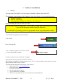
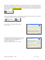

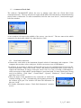
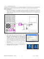
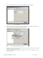
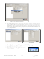
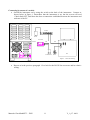
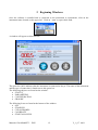
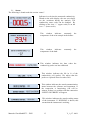
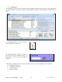
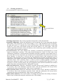
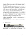
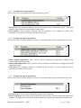
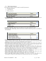
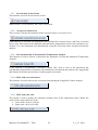
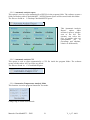
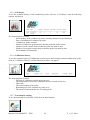
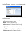
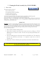
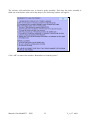
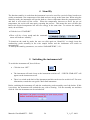

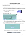
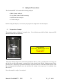
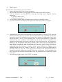
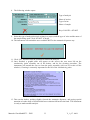
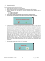
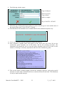
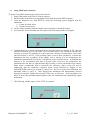
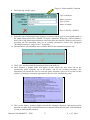
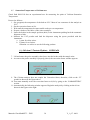
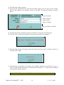
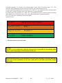
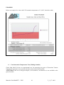
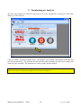
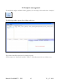
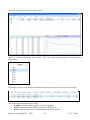
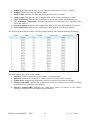
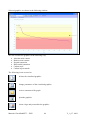
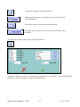
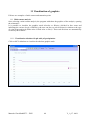
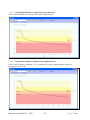
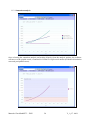
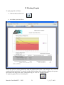
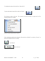
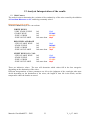

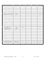
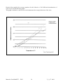
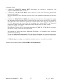
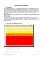

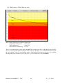
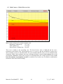
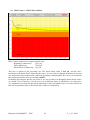
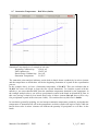
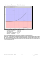
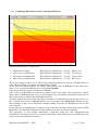
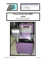

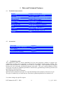
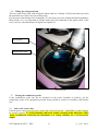
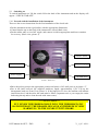
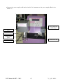
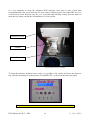
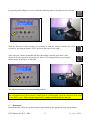
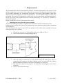
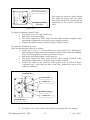
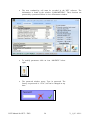
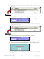


![j:j_"Xt$l"j:]:":,lg]:"r/Human Resources have been duty - e](http://vs1.manualzilla.com/store/data/005657435_1-26d97049bf04f0fd92265d73e45a9ab3-150x150.png)