Download Sim3DMax User Manual

Contents
1 System requirements
6
2 Installing the FDTD program to hard disk
7
3 Command line arguments
8
4 Parameter File Description
4.1 Simulation name . . . . . . . . . . . . . . . . . . . .
4.2 Time control . . . . . . . . . . . . . . . . . . . . . . .
4.3 Spatial grid specification . . . . . . . . . . . . . . . .
4.4 Computations in 2D . . . . . . . . . . . . . . . . . .
4.5 Working Directory . . . . . . . . . . . . . . . . . . .
4.6 Material Definition File . . . . . . . . . . . . . . . . .
4.7 Geometry Definition File . . . . . . . . . . . . . . . .
4.8 Boundary Conditions File . . . . . . . . . . . . . . .
4.9 Material index output . . . . . . . . . . . . . . . . .
4.10 Field output . . . . . . . . . . . . . . . . . . . . . . .
4.11 Checkpoint files . . . . . . . . . . . . . . . . . . . . .
4.12 Source time profile . . . . . . . . . . . . . . . . . . .
4.13 Sources . . . . . . . . . . . . . . . . . . . . . . . . . .
4.14 DIFFRACTTM source specification . . . . . . . . . .
4.15 Point source specification . . . . . . . . . . . . . . . .
4.16 Planewave source specification . . . . . . . . . . . . .
4.17 Gaussian beam source specification . . . . . . . . . .
4.18 2D source specification from the file . . . . . . . . . .
4.19 2D planar waveguide source specification . . . . . . .
4.20 File format version compatibility with DIFFRACTTM
4.21 Coordinate system transformation . . . . . . . . . . .
4.22 Export file specification . . . . . . . . . . . . . . . . .
4.22.1 Export of the reflected field . . . . . . . . . .
4.22.2 Export of the transmitted field . . . . . . . .
4.23 Monitor header comment . . . . . . . . . . . . . . . .
4.24 Monitor specification . . . . . . . . . . . . . . . . . .
4.24.1 Monitors for computations in 2D . . . . . . .
4.24.2 Monitors for computations in 3D . . . . . . .
2
.
.
.
.
.
.
.
.
.
.
.
.
.
.
.
.
.
.
.
.
.
.
.
.
.
.
.
.
.
.
.
.
.
.
.
.
.
.
.
.
.
.
.
.
.
.
.
.
.
.
.
.
.
.
.
.
.
.
.
.
.
.
.
.
.
.
.
.
.
.
.
.
.
.
.
.
.
.
.
.
.
.
.
.
.
.
.
.
.
.
.
.
.
.
.
.
.
.
.
.
.
.
.
.
.
.
.
.
.
.
.
9
10
10
11
15
16
16
16
16
17
17
21
22
23
24
25
26
30
33
35
36
37
39
39
40
42
42
44
46
5 Boundary Conditions File Description
46
6 Material File Description
6.1 Dielectric materials . . .
6.2 Debye model . . . . . . .
6.3 Lorentz model . . . . . .
6.4 Drude model . . . . . .
6.5 Magnetic material model
.
.
.
.
.
48
49
50
54
55
55
.
.
.
.
.
.
.
.
.
.
.
.
.
.
.
.
.
57
57
58
58
59
59
59
60
60
60
62
63
66
66
70
72
73
74
.
.
.
.
.
.
.
.
.
.
.
.
.
.
.
.
.
.
.
.
.
.
.
.
.
.
.
.
.
.
.
.
.
.
.
.
.
.
.
.
.
.
.
.
.
.
.
.
.
.
.
.
.
.
.
.
.
.
.
.
.
.
.
.
.
.
.
.
.
.
.
.
.
.
.
.
.
.
.
.
.
.
.
.
.
.
.
.
.
.
.
.
.
.
.
7 Geometry File Description
7.1 Geometry specification from an input file . . . . . . . . . .
7.2 Basic Geometric primitives . . . . . . . . . . . . . . . . . .
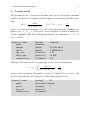
7.2.1 Sphere . . . . . . . . . . . . . . . . . . . . . . . . .
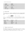
7.2.2 Cube . . . . . . . . . . . . . . . . . . . . . . . . . .
7.2.3 Ellipsoid . . . . . . . . . . . . . . . . . . . . . . . .
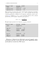
7.2.4 Cone . . . . . . . . . . . . . . . . . . . . . . . . . .
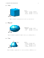
7.2.5 Disk . . . . . . . . . . . . . . . . . . . . . . . . . .
7.2.6 Polygon . . . . . . . . . . . . . . . . . . . . . . . .
7.2.7 Ellips . . . . . . . . . . . . . . . . . . . . . . . . .
7.2.8 Lattice . . . . . . . . . . . . . . . . . . . . . . . . .
7.2.9 Pattern . . . . . . . . . . . . . . . . . . . . . . . .
7.3 Geometric objects for optical data storage media modeling
7.3.1 Bumps/pits . . . . . . . . . . . . . . . . . . . . . .
7.3.2 Grooves . . . . . . . . . . . . . . . . . . . . . . . .
7.3.3 Conformal layer . . . . . . . . . . . . . . . . . . . .
7.3.4 Sine-layer . . . . . . . . . . . . . . . . . . . . . . .
7.4 Dielectric Material Interfaces . . . . . . . . . . . . . . . . .
8 Comments in the input files
74
9 Application Examples
9.1 Order of convergence . . . . . . . . . . .
9.2 Reflection from a bi-layer . . . . . . . . .
9.3 Scattering of a planewave from a sphere
9.4 Laser beam scattering from a mark . . .
9.5 Imaging problem . . . . . . . . . . . . .
75
75
76
78
79
85
3
.
.
.
.
.
.
.
.
.
.
.
.
.
.
.
.
.
.
.
.
.
.
.
.
.
.
.
.
.
.
.
.
.
.
.
.
.
.
.
.
.
.
.
.
.
.
.
.
.
.
.
.
.
.
.
Appendices
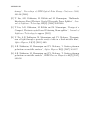
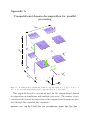
A Computational domain decomposition for parallel processing
B Parallel performance and load balancing . . . . . . . . . . . .
C Staggered field location for user-defined sources . . . . . . . .
D Monitor file formats . . . . . . . . . . . . . . . . . . . . . . .
E Article reprints . . . . . . . . . . . . . . . . . . . . . . . . . .
4
.
.
.
.
.
96
96
98
101
103
105
Sim3D MaxTM FDTD code User Manual
November 29, 2009
This document describes the user interface to a software module for solution of the time dependent vector Maxwell equations in three dimensions
using the Finite Difference Time Domain (FDTD) method [1]. The main
features of the program are:
•
•
•
•
•
•
•
•
full vector field description in 3-D Cartesian geometry
computation speed-up with AccelewareTM hardware
compatibility with DIFFRACTTM software
non-uniform grid support
non-dispersive and dispersive material models
UPML absorbing boundary conditions
arbitrary geometry input
parallel implementation for multi-processor platforms,
based on the Message Passing Interface (MPI) [2] standard
Maxwell’s equations, along with the constitutive relations, are discretized
in space and time using FDTD method based on the second-order accurate,
staggered central-difference operators. In MKS units the relevant equations
can be written as follows:
∂D
= ∇ × H − σE,
∇ · D = 0,
∂t
∂B
= −∇ × E,
∇ · B = 0,
∂t
∂P
D = 0 E + P, B = µ0 H, Jp =
,
∂t
where E [Volts/m] is the electric field, D [Coulombs/m2 ] - electric flux den5
1
SYSTEM REQUIREMENTS
6
sity, H [Amperes/m] - magnetic field, B [Webers/m2 ] - magnetic flux density,
Jp [Amperes/m2 ] - electric polarization current density and P [Coulombs/m2 ]
is the electric polarization vector. Material properties are defined by electric conductivity σ [1/(Ohm m)], permittivity = 0 r and polarization P,
where 0 = 8.854×10−12 [Farads/m] and µ0 = 4π ×10−7 [Henrys/m] are freespace electric permittivity and magnetic permeability, and r is the relative
permittivity.
The version of the program described in this document allows computation of the scattered field for a given structure and a given incident field
distribution created in DIFFRACTTM [3]. The input and output file formats
are compatible with the file formats used by the FDTD interface option of
the DIFFRACTTM software.
Sections 1 and 2 provide information on the system requirements and installation. Section 3 describes command line arguments of the program. In
section 4 the structure of the input parameter file is given. Boundary conditions, material model and geometry input are described in sections 5-7. The
last section provides some example problems along with the corresponding
input files.
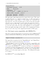
1
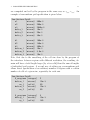
System requirements
Binary executables of the program are available for IA32 and EM64T/AMD64
platforms running Windows NT/2000/XP or XP x64 operating systems.
Hardware acceleration is supported for Windows 2000/XP Pro/XP Pro x64
operating systems and requires a PCI Express x16 slot(s) for the Acceleware
AcceleratorTM card(s).
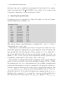
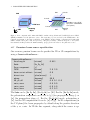
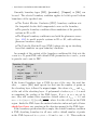
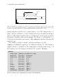
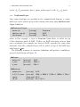
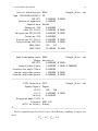
Table 1: Supported architectures and WindowsTM operating systems.
ABI/OS
×32
×64
NT,2000
•
•
XP Pro
•
•
XP Pro with AccelewareTM
•
•
Compute Cluster Server 2003 x64
•
•
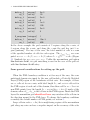
An Intel PentiumTM 4, AMD Opteron (or equivalent) 1GHz or better processor and 1Gbyte or more of random access memory are recommended. The
lower bound on the memory (in bytes) required by any given problem, can
be estimated with the following formula: M = Nx × Ny × Nz × Nv × Nf ,
2
INSTALLING THE FDTD PROGRAM TO HARD DISK
7
where Nx , Ny , Nz are the number of points along the x, y, z axis and Nv is
the number of variables stored at each point. The value of Nv is 6 (for E and
H vector fields) if only dielectric material model is used and Nv = 6 + 3p (E
and H plus polarization vectors) if a dispersive Debye material model with
p poles is used, or Nv = 9 + 6p for the dispersive materials described by the
Lorenz or Drude model with p poles (see section 6). The number of variables
doubles when the Floquet boundary conditions are used. The factor Nf in
the formula equals 4 bytes per float number for single precision and Nf = 8
for double precision. For example, an application that uses only a dielectric
material model, boundary conditions other than Floquet and 200×200×100
grid points, will require about 200Mbytes of memory.
Binary executables of the program for parallel computations take advantage
of the many CPUs in the multiple-processor workstations, or a cluster of
workstations connected by a high speed communication network. The execution time and memory requirements per node are reduced by distributing
the computation across many nodes. For both serial and parallel execution
of the program, the MPI libraries must be installed on the system. Support
for the MicrosoftTM MPI based High Performance Compute Cluster systems (Compute Cluster Server 2003 x64) as well as for the freely available
MPICH2 based systems, is included. A freely available implementation of
the MPI standard for Windows NT4/2000/XP Professional/XP Professional
x64 or Server can be found on the installation disk or can be downloaded
from the Argonne National Laboratory web site [2].
2
Installing the FDTD program to hard disk
To install the Finite Difference Time Domain (FDTD) program Sim3D MaxTM
on hard disk, load the distribution CD-ROM. Double-click on Setup to start
the installation (requires administrator priviledges). In addition to the setup
of the Sim3D MaxTM package, the Setup utility will also invoke the installers
for the following packages1 :
• Message Passing Interface MPICH2TM system;
• AccelewareTM drivers (if applicable);
1 Installation
of the Message Passing Interface system is required for single- as well as multi-processor systems.
3
COMMAND LINE ARGUMENTS
8
• SafeNet SentinelTM USB license key drivers.
Choose “Reboot later” option during installation of each of the above
components, and reboot only once, after the Setup finishes. Upon successful
completion the installation creates a directory named
<NLCST\Sim3D Max\Version.Number\>
under <Program Files> folder, and places a shortcut to the Sim3D MaxGUI
executable on the Desktop. Within the installed directory you will find the
following folders: <GUI>, <Bin>, <Docs>, <Examples>.
<GUI> - supporting files for the Graphical User Interface of the program
<Bin> - Sim3D MaxTM executables and supporting files
<Docs> - manuals, publication reprints, and other documentation
<Examples> - folders with sample input files and test cases.
Follow instructions in Readme.pdf to complete the installation. For the
computations that use the DIFFRACTTM source, the input beam, i.e. the
complex light amplitude distribution that enters the FDTD mesh, must be
generated by DIFFRACTTM (using the menu option FDTD in Export mode),
then imported to the Sim3D Max.exe. All output distributions computed by
Sim3D Max.exe will be stored on hard disk in files within the working directory specified in the parameter input file of Sim3D Max.exe. Subsequently,
these output files may be imported by DIFFRACTTM (using the menu option
FDTD in Import mode) and displayed (using the option PLOT) or processed
as any other beam cross-section is processed in DIFFRACTTM .
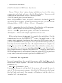
3
Command line arguments
For serial computations the executable program, called Sim3D Max, can be
invoked with a single argument – the name of a text file containing simulation
parameters, e.g.
Sim3D Max parameters.input
If parameter filename is not specified, the program will prompt the user to
enter it. To do many runs in sequence, batch files (in Windows) or shell script
files (in Unix) can be used. For example, in Windows a text file called, e.g.
“simulate.bat” containing lines
4
PARAMETER FILE DESCRIPTION
9
Sim3D_Max parameters1.input -b
Sim3D_Max parameters2.input -b
...
Sim3D_Max parametersN.input
can be executed to perform unattended N simulations with different parameters. The switch -b at the end of the command lines prevents the batch
job from stopping at the end of each run or in case error conditions are
encountered.
For parallel runs the program is invoked using MPI launcher and takes, in
addition to the input parameter file name, an optional list of three integer
numbers. These numbers specify the desired number of processing elements
(CPUs or threads) per x, y, z dimension of the computational domain (see
Appendix A Figure 35 for details). For example to start a run on six processors, and default distribution of processing elements, use
mpiexec.exe -np 6 Sim3D_Max.exe parameters.input
To assign one processor along the x-axis, three - along the y-axis and two along the z-axis, use
mpiexec.exe -np 6 Sim3D_Max.exe parameters.input 1 3 2
The choice of processor grid, load balancing issues and parallel performance
on different platforms are discussed in Appendix B.
The AccelewareTM hardware-accelerated runs can be launched by specifying on the command line the option “-acceleware auto”, e.g.:
Sim3D_Max.exe C:\somedir\parameters.input -b -acceleware auto
This executes computations using AccelewareTM hardware that speeds up the
computations, with automatic selection of the processing option for optimal
performance.
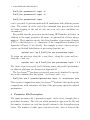
4
Parameter File Description
The input parameter file (“parameters.input” in the above example) has a
predefined structure. The order in which parameters appear in the file and
the number of entries on each line should conform to the description given
below. The number of white space characters before, after or between the
4
PARAMETER FILE DESCRIPTION
10
entries on each line and the number of newline characters between lines can
be arbitrary. The entry here means a sequence of characters not separated
by a white space, tab, newline or carriage-return character. For example, if
the manual shows x0,y0,z0, then DO NOT use x0, y0, z0 instead.
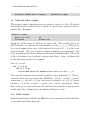
4.1
Simulation name
The first line should be a line consisting of three arbitrary words. It can be
used to describe the file or simulation. Example:
FDTD Input Parameters
4.2
Time control
Time control specifies the start and finish times for the simulation in nanoseconds and sets the time step, e.g.:
Start-stop and timestep:
tmin [nanoseconds] 0.0
tmax [nanoseconds] 20.0e-6
delta_t automatic-with-CFL 0.4
The time step, delta t, can be set in two ways. The first format,
delta t automatic-with-CFL CFL NUMBER
specifies that the time step should be computed from the spatial grid cell
sizes, ∆x, ∆y, ∆z according to,
dt = CF L N U M BER × min(∆xi , ∆yj , ∆zk )/c,
where c is the speed of the light in a vacuum and CFL number
√ should be a
number less than the stability limit, CF L N U M BER < 1/ 3.
The second format,
delta t [nanoseconds] 1.0e-8
sets the value of the time step explicitly, in nanoseconds.
For problems in which time-harmonic (continuous-wave) solution is sought,
the convergence of the solutions can be verified by increasing the value of
tmax with all other problem parameters unchanged, and repeating the simulation. Similarly, convergence of the solution with respect to the value of
4
PARAMETER FILE DESCRIPTION
11
the time step can be verified by decreasing the time step ∆t (or, equivalently, decreasing the CF L N U M BER). See section 4.3 for accuracy and
convergence dependence on the spatial grid cell size.
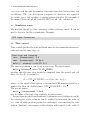
4.3
Spatial grid specification
A uniform grid can be specified by setting the number of cells and computational domain size as follows, e.g.:
Uniform Grid:
nx
[cells]
ny
[cells]
nz
[cells]
xmin
[micron]
xmax
[micron]
ymin
[micron]
ymax
[micron]
zmin
[micron]
zmax
[micron]
120
150
200
-3.0
5.0
-6.0
4.0
0.0
15.0
The cell size along x axis will then be a constant ∆x = (xmax − xmin )/nx ,
and similarly for y and z axis.
Alternatively, a non-uniform grid can be set up in one of the two ways.
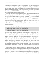
In the first approach, appropriate for grids symmetric in the XY -plane, the
user specifies the sizes (in micron) of three regions, w1 , w2 , w3 along the x
(or y) axis, followed by the cell sizes in each of these regions ∆1 , ∆2 , ∆3 , see
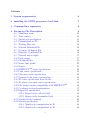
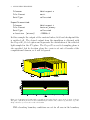
Figure 1a. The x and y axis are treated identically and the generated grid
is symmetric with respect to the center of the x and y axis.
The cell sizes are interpolated at the boundaries of the regions with different cell sizes to provide a grid with gradually changing cell size. Unlike
the uniform grid case, for a non-uniform grid, the resulting computational
domain size and number of cells are computed by the program, and the coordinate origin is positioned at the center of the computational domain. The
xmax , xmin and ymax , ymin values are set by the program to ±Lx /2, ±Ly /2 respectively, where Lx , Ly are the total domain size computed from w1 , w2 , w3 .
Similarly, three regions h1 , h2 , h3 along the z axis are specified, followed by
the cell sizes in each of these regions, ∆z1 , ∆z2 , ∆z3 , Figure 1a. The zmin , zmax
4
PARAMETER FILE DESCRIPTION
12
a)
Zmax= Lz/2
Lx
nz_PML
h3, ∆z3
nx,y_PML
Z
Lz
h2, ∆z2
Zmin=-Lz/2
w3, ∆3
w2, ∆2
h1, ∆z1
w3, ∆3
w2, ∆2
w1, ∆1
X (or Y)
Xmin=-Lx/2
b)
Xmax=Lx/2
N
Ly
nx1
Nzregions
nz4
nz3
nz2
Z
nz1
ions
∆x1
∆x2
nx2
∆z4
ny3
ny2
ny1
∆z3
∆y2
∆y3
Lz
∆y1
∆z2
∆z1
Y
X
xreg
Lx
N yregions
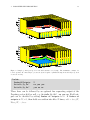
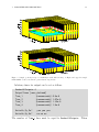
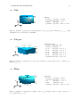
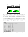
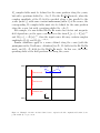
Figure 1: a) Computational domain and non-uniform grid definition for the Non-Uniform Grid1 input.
The grid is symmetric in the XY plane and consists of three regions with different cell sizes along either x, y
or z-axis. b) Computational domain and non-uniform grid definition for the Non-Uniform Grid2 input.
The grid consists of arbitrary number of regions with different cell sizes along the x, y and z-axis. In the
example shown Nxregions = 2, Nyregions = 3, Nzregions = 4. The total number of cells along any axis is
equal to the sum of the specified number of cells in each region of that axis. When absorbing BCs are set,
PML regions are always counted as part of the total length of the domain.
4
PARAMETER FILE DESCRIPTION
13
are computed and set by the program in the same way as xmin , xmax . An
example of non-uniform grid specification is given below:
Non-Uniform Grid1:
w1
[micron]
w2
[micron]
w3
[micron]
delta_1
[micron]
delta_2
[micron]
delta_3
[micron]
h1
h2
h3
deltaz_1
deltaz_2
deltaz_3
[micron]
[micron]
[micron]
[micron]
[micron]
[micron]
500e-3
200e-3
2040e-3
10e-3
20e-3
30e-3
160e-3
140e-3
300e-3
10e-3
5.0e-3
10e-3
Note, that due to the smoothing of the cell size done by the program at
the interfaces between regions with different resolution, the resulting domain will have a total length larger (by a few cells) than the sum of lengths
of individual grid regions. A second way of setting up a non-uniform grid
allows direct specification of an arbitrary number of regions with a certain
number of cells of a given size, separately for each axis.
Non-Uniform Grid2:
N_xregions [integer]
deltax_1
[micron]
nx_1
[cells]
deltax_2
[micron]
nx_2
[cells]
2
10e-3
50
10e-3
50
N_yregions [integer]
deltay_1
[micron]
ny_1
[cells]
5
10e-3
185
4
PARAMETER FILE DESCRIPTION
deltay_2
ny_2
deltay_3
ny_3
deltay_4
ny_4
deltay_5
ny_5
[micron]
[cells]
[micron]
[cells]
[micron]
[cells]
[micron]
[cells]
N_zregions [integer]
deltaz_1
[micron]
nz_1
[cells]
14
5e-3
10
2e-3
5
1e-3
150
2e-3
5
1
10e-3
400
In the above example the grid consists of 2 regions along the x-axis, of
5 regions along the y-axis, and along the z-axis the grid has just 1 region (uniform). For any of the axes, the total number of cells is a sum
of the specified number of cells for each region. The xmin , xmax , are comPNxregions
puted as xmin = −Lx /2, xmax = Lx /2, where Lx = i=1
nxi ∆xi (Figure
1). Similarly for ymin , ymax ,zmin , zmax . Unlike the non-uniform grid option
Non-Uniform Grid1, no grid smoothing is used in the case of the grid set
with Non-Uniform Grid2 entry.
Some general considerations for setting up the grid:
When the PML boundary condition is set for any of the axes, the computational domain size input by the user will include a Perfectly Matched
Layer (PML) region at the boundaries of that axis. For example, if there
are nx cells set for an x-axis, with total length Lx , and nxP M L cells set for
the PML region at each end of the domain, then there will be nx − 2nxP M L
non-PML points (over the length Lx − nxP M L (dxtop + dxbot )) inside of the
domain, where dxtop , dxbot is the cell size in the PML regions. Inside the PML
layers the nonuniform grid should not have any variation of the cell size in
the direction normal to the PML layer. To change the boundary conditions
or modify the default number of PML points, see section 5.
Large cell-size ratio r = ∆1 /∆2 in neighboring regions of the non-uniform
grid along any axis can have a negative impact on the accuracy of the solu-
4
PARAMETER FILE DESCRIPTION
15
tion. Gradual change of the cell size must be used when a ratio of cell size
r > 2 is used for grid refinement. Additionally, large cell-size aspect ratios
∆u /∆v , u, v = x, y, z must be avoided to maintain accuracy.
The grid cell-size along any axis and within a region of material with
refractive index nref , can be estimated as ∆ ≤ λ/(Nppw nref ), where λ is
the free space wavelength of interest, and Nppw is the number of cells per
wavelength in the medium. Typically, for errors in the solution to be less
than a few percent, Nppw > 20−30 must be used. The computation time step
is proportional to the smallest cell size found in the computational domain.
Convergence of the solutions can be verified by decreasing the cell sizes,
typically by a factor of 2, with all other problem parameters unchanged, and
repeating the simulation.
4.4
Computations in 2D
The default computation mode is 3D. In order to switch to two-dimensional
computations, either uniform grid or second approach to the non-uniform
grid specification must be used to set the number of points in the x-direction
to nx=1 and the boundary condition for the xaxis must be defined as
[periodic] in the boundary conditions file, described in section 5. One
of the 2D sources must be specified for (Hx Ey Ez) or (Ex Hy Hz) mode
computation (sources are described in subsection 4.13).
With nx set to 1, the 2D computational domain is the Y Z-plane and the
2D modes are the transverse electric T Ex → (Hx , Ey , Ez ), and transverse
magnetic T Mx → (Ex , Hy , Hz ) modes, with field components depending on
time and y, z coordinates: E = E(t, y, z) and H = H(t, y, z). Hence, this
manual uses the convention, in which T Ex (or T Mx ) signifies the mode with
electric (or magnetic) field transverse to the x-axis.
For 2D computations the domain in the x-direction is just one cell long
and can have arbitrary coordinates xmin , xmax of the computational domain.
A convenient choice of xmin , xmax usually is xmin = 0 and xmax equal to
the largest cell size along the y or z axis. All source, monitor, geometry,
etc. objects, that require input of an x-coordinate must use values within
the xmin < x < xmax range, if positioning in the Y Z-plane of the
computational domain is desired.
4
PARAMETER FILE DESCRIPTION
16
Working Directory
4.5
The working directory is a full pathname specifying a directory where the
program will look for all input (geometry, material, boundary conditions,
source) files, and where it will write the output files, e.g.,
Working directory:
/home/username/Maxwell/FDTD/
Working directory:
C:\username\Maxwell\FDTD\
or
For all input files the program looks for the file (e.g. file material.input
described in the next subsection) in the directory specified under Working
directory:. However, if the filename includes explicitly the path,
C:\User\myfiles\material.input
or
.\material.input
then the filename is used as specified. Directory and file names containing
the space character must be enclosed by double-quote characters: “C:\User
Name\My Data Files\”.
4.6
Material Definition File
The “Material Definition File” sets a filename of a file containing material
model specifications (see section 6), e.g.
Material Definition Filename:
4.7
material.input
Geometry Definition File
The “Geometry Definition File” sets the filename of a file containing geometry specifications (see section 7), e.g.
Geometry Definition Filename:
geometry.input
Same rules regarding filename apply as specified above.
4.8
Boundary Conditions File
Boundary conditions can be set using the file specified under the Boundary
Conditions Filename: entry (see section 5). For example:
4
PARAMETER FILE DESCRIPTION
17
Boundary Conditions Filename:
4.9
boundaries.input
Material index output
The material index output provides an option to write to a file a 3D spatial
distribution of the material logical index set up from the material and geometry files. Example:
Material index:
Write to file?
Filename
no
mindex.out
Write to file? must be followed by yes or no. The resulting file is in
ASCII format. It contains the total number of cells nx , ny , nz , followed by
the logical enumeration value of the material for each cell i, j, k of the computational grid. This logical value is simply a number corresponding to the
order in which materials are defined in the material definition file. The order
of the cell output is one, in which k changes first, then j, then i, as illustrated
in the following pseudo-code segment:
for i=1 to nx
for j=1 to ny
for k=1 to nz
write/read material enumeration value in cell i,j,k
The same file structure is used in the geometry object defined in 7.1. The coordinates of the cells are written into ASCII files “coordx”, “coordy”,“coordz”
in microns, i.e. the cell i, j, k has cell-center coordinates x[i], y[j], z[k] found
on lines i, j, k in files “coordx”, “coordy” and “coordz” respectively. These
files can be used to plot and verify the material and geometry setup specified
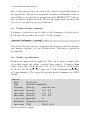
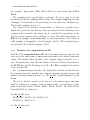
in the input files. Sample plots are shown in Figures 2 and 3.
4.10
Field output
Spatial distribution of the E and H fields can be optionally written into files
at specified equal time intervals:
4
PARAMETER FILE DESCRIPTION
18
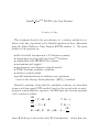
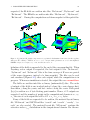
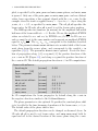
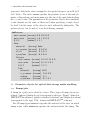
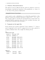
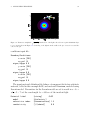
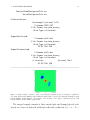
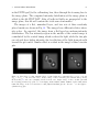
Figure 2: Sample geometry set-up for a near field antenna over a bump. The transmitter consists of a
bow-tie aperture in a metal layer ( cross-section) and a sphero-cylindrical bump in another layer (bottom
cross-section view).
Fields:
NumberOfOutputs
WriteEx,Ey,Ez?
WriteHx,Hy,Hz?
2
no yes yes
yes no no
These lines can be followed by an optional line requesting output of the
Poynting vector field as well, e.g: WriteSx,Sy,Sz? no yes no. Field output can be disabled by setting Number of outputs to 0. If Number of
outputs is N > 0, then fields are written into files N times, at t = tmax /N ,
2tmax /N , ..., tmax .
4
PARAMETER FILE DESCRIPTION
19
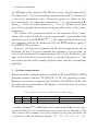
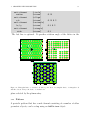
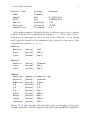
Figure 3: Sample geometry set-up of a multi-layer stack with an array of elliptic and capped-rectangle
marks similar to those used in the optical data storage media.
Arbitrary times for output can be set as follows:
NumberOfOutputs 4
OutputTimes [user_defined]
Time_1
[nanoseconds]
Time_2
[nanoseconds]
Time_3
[nanoseconds]
Time_4
[nanoseconds]
WriteEx,Ey,Ez?
WriteHx,Hy,Hz?
0.8e-6
1.07e-6
1.35e-6
1.8e-6
yes yes yes
no no no
The number of Time i lines must be equal to NumberOfOutputs. When
4
PARAMETER FILE DESCRIPTION
20
requested, the E fields are written into files “Ex.bin.out”,“Ey.bin.out” and
“Ez.bin.out”. The H fields are written into files “Hx.bin.out”, “Hy.bin.out”,
“Hz.bin.out”. During the computation each time-snapshot of the spatial dis-
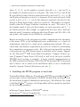
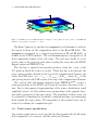
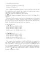
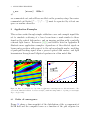
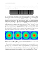
Figure 4: Ey (left) and Ez (right) components of a y-polarized 3D Gaussian beam sourced in the xy-plane
with periodic boundary conditions, at zmin = zmax = 0.7µm with z-parameter set to 0, beam amplitude
FWHM= 1.2µm, λ0 = 0.8µm, nref = 1.0, and direction set to -1.
tribution of the fields is appended to the end of the corresponding file. When
Poynting vector output is requested, the last output to the “Sx.bin.out”,
“Sy.bin.out” and “Sz.bin.out” files is the time average of S over one period
of the source frequency, instead of a time-snapshot. The files can be read
and visualized (Figures 4-5) after each output, while the computation is in
progress. When new simulation is started, the output files are overwritten.
The fields are written into files as binary (unformatted) data. The order
of output of the fields is one in which index k along the z-axis changes first,
then index j along the y-axis, and last - index i along the x-axis. Each point
(k,j,i) is written as a 4 byte floating point number. Hence, if N outputs are
requested, and the number of points in the computational domain is nx , ny ,
nz , the size of each output file will be 4N × nx × ny × nz bytes.
If any of the fields are requested to be written, the material layout binary
file “Ml.bin.out” and ASCII text files “coords” and “coordx”, “coordy”, “coordz” are also created. The material layout file “Ml.bin.out” contains the
refractive index nref distribution in the computational domain. For the ma-
4
PARAMETER FILE DESCRIPTION
21
Figure 5: Sy ,Sz components of a 3D Gaussian beam from Fig. 4.
terials based on Lorentz and Debye material models, instead of nref a value
−m is written into “Ml.bin.out” file, where m is the order number in which
the material is defined in the material definition file. For the materials of
type Debye(x,y) the conductivity (in MKS units) is used in the “Ml.bin.out”
file for each point of the domain occupied by the Debye(x,y) materials. The
binary data format of the material layout file is the same as that of the field
files.
The file “coords” contains on the first line the number of points, nx , ny ,
nz , followed on the second line by the number N of outputs done, and the
computation output times, in seconds, e.g. t = tmax /N , 2 ∗ tmax /N , ..., tmax ,
on the third and following lines. The files “coordx”, “coordy”, “coordz”
contain a single column corresponding to the coordinates of each cell in the
x,y,z direction.
4.11
Checkpoint files
The CheckpointFile: block sets the file output and input options for saving and restarting the computation. RestartFromCheckpointFile option
allows the computation to be continued from a previously saved checkpoint
file. WriteCheckpointFile requests that a checkpoint file be created at the
4
PARAMETER FILE DESCRIPTION
22
end of simulation.
CheckpointFile:
RestartFromCheckpointFile
WriteCheckpointFile
no
yes
Each processor creates one checkpoint file in the working directory under
filename “chkpLxMxN”, where L,M,N are integers identifying the processor.
If the checkpoint file already exists, it is overwritten.
When simulation is restarted from the checkpoint file, the program assumes that the material and geometry definition files are the same as those
used in the run that created the checkpoint file. Also, start time tmin is
reset to the simulation time read from the checkpoint file, and tmax is set to
the new tmin plus the difference between tmax and tmin appearing in the
input parameters file. All other time dependent entries in the parameter file
are used as specified.
When monitors or ExportReflected/Transmitted planes are used with the
checkpoint option, the Fourier transforms and monitored fields are not saved
to the checkpoint files, and hence they do not persist from one checkpoint
to another. Instead, they are computed anew in every run. Therefore, for
example, the data in the Export plane files from any run is valid only if the
simulation time tmax−tmin of that particular run is large enough to sample
the minimum required number of periods of the source, otherwise a warning
message is issued by the program.
4.12
Source time profile
The TimeProfile: block is optional in the input file. When present, it specifies the modulation f (t) of the time dependent source f (t) sin(ωt + φceo ):
TimeProfile:
f(t) [superGaussian]
t0
[nanoseconds]
400.0e-6
FWHM [nanoseconds]
80.0e-6
n
2.0
Valid options for the f(t) entry are [sech], [superGaussian], [tanh]
or [file]. The functional dependence and parameter values for these op-
4
PARAMETER FILE DESCRIPTION
23
tions are given in the Table 2. The default time profile is a tanh function,
with t0 set to 3 fs, and tau - to 1 fs. In the case of a user defined time profile,
TimeProfile:
f(t)
[file]
Filename
[string]
user_time_profile.input
the specified ASCII file is expected to contain on the first line the number of points, Nt , present in the file, followed by a single column of the
values of the function f (t) sampled at each computation time step t = i · dt,
i = 1, 2, .... During the simulation, for t > Nt · dt, the f (t) is set to the value
on the last line of the input file.
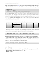
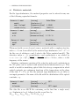
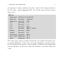
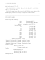
Table 2: Source time profile parameters
f(t)
Function
Parameter 1
Parameter 2
[sech]
[superGaussian]
[tanh]
[file]
2
exp[−(t−t0 )/τ ]+exp[(t−t0 )/τ ]
exp[−{(t − t0 )/τ }n ]
1
2 (1 + tanh[(t − t0 )/τ ])
t0
t0
t0
filename
FWHM = 2τ ln(2 + 3)
FWHM = 2τ (ln 2)1/n
tau=τ
—
user defined
√
Parameter 3
—
n
—
—
For any choice of the profile, the amplitude of the time profile function
can be set by specifying an optional entry in the following form:
amplitude
[V/m]
2.0
-or-
amplitude
[A/m]
2.0
If this line is omitted, a default value of 1.0 is assumed for the amplitude.
The default value of the phase-shift between the envelope function f (t)
and the carrier wave sin(ωt + φceo ) is zero, φceo = 0. The carrier-envelope
offset φceo can be changed with an optional entry:
carrier-envelope offset
4.13
[degrees] -90.0
Sources
One of the following sources must be specified in the input parameters file:
• source from the input DIFFRACTTM file
• point source
4
PARAMETER FILE DESCRIPTION
•
•
•
•
24
planewave source
Gaussian beam source
source from the input file in 2D
planar waveguide source in 2D
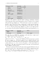
Sub-sections 4.14-4.19 describe input required for each of these sources.
4.14
DIFFRACTTM source specification
To use a DIFFRACTTM source the user must set the wavelength (in microns), the filename (see 4.5 for input filename rules) of a complex-valued
source amplitude distribution for E and H fields, the format of the file and
the grid type. For a beam propagating in DIFFRACTTM along the positive
direction of the z-axis, H-fields must be sampled on a plane positioned a
distance ∆z /2 (half of a FDTD grid cell) behind the plane where E-fields
are sampled, Figure 6. Therefore, negative value of −∆z (not −∆z /2) must
be specified when the source file is produced by the FDTD export option of
DIFFRACTTM . The content and format of the file are described in detail in
section 4.20 and in the manual for the DIFFRACTTM software [3]. Either
Source: or DiffractSource: may be used to specify a source distribution created with DIFFRACTTM . The File Format can be one of ascii,
fortran binary, c binary. The choice ascii is used for files in a text format as produced by FORTRAN for type COMPLEX.
DiffractSource:
Wavelength [micron]
Filename
File Format
Grid Type
z-location [micron]
0.65
diffract_output.dat
ascii
staggered
0.1
The fortran binary format corresponds to unformatted output produced
by FORTRAN and is the same as the binary format used in DIFFRACTTM .
The option c binary is for the binary output produced for/by C programs.
The later is different from FORTRAN in that it does not have data tags, and
elements of the arrays are written in the row-major order. Binary format
allows smaller file size and faster data input or output, than does ASCII.
4
PARAMETER FILE DESCRIPTION
25
z
E(x,y)
∆ z/2
H(x,y)
Figure 6: In Diffract source file E-fields must be sampled on an xy-plane at some position z, with H-fields
sampled on an xy-plane at position z − ∆z/2.
The Grid Type can be specified as staggered or collocated, to indicate
the logical location on the computation mesh of the E and H fields. The
staggered corresponds to a staggered positioning of E and H fields, as
defined in the FDTD method. The collocated option corresponds to all
field components defined at the cell center. The grid type should be set to
be the same as the grid type used when creating the source file with FDTD
Export option in DIFFRACTTM .
The last line is optional and specifies position, along the z-axis, of the
XY -plane in which the source is excited. When this line is not present, the
source plane position defaults to the top of the computational domain, just
before the PML layer, at z = zmax − (nz P M L + 3)∆ztop , where ∆ztop is the
grid spacing used in the PML region at the top of the computational domain.
The sourced field distribution imported from DIFFRACTTM , creates a
beam propagating in the FDTD grid along the negative direction of the zaxis. Due to the numerical approximation of the source distribution, small
amplitude (about -30 db) residual waves propagating in the opposite direction will be generated at the source plane. The magnitude of these waves can
be evaluated by launching the beam into a uniform medium, and monitoring
fields behind the source plane. The magnitude of the residual waves can be
reduced by refining the computation grid.
4.15
Point source specification
One or more point sources can be specified by their position x0,y0,z0, single
field component to be sourced, and the switch on/off times.
4
PARAMETER FILE DESCRIPTION
PointSource:
Wavelength
x0,y0,z0
E-field
t_on,t_off
phase
[micron]
[micron]
[x]
[nanoseconds]
[degrees]
26
0.65
0.0 0.0 100e-3
1.0e-6 6.0e-6
90
The phase parameter is optional. It specifies the constant phase shift φ0
to be added to the time harmonic dependence of the point source, ωt + φ0 .
When not specified, the phase shift defaults to zero.
The valid options for the field component entry are E-field followed by
one of the [x], [y] or [z] for computations in 3D. For 2D Hx Ey Ez mode,
E-field components [y] or [z], or H-field component [x] can be specified. For 2D Ex Hy Hz mode, H-field components [y] or [z], or E-field
component [x] can be specified. At each time step of the computation the
value of the specified field component at the source location (single grid point
rps = (x0 , y0 , z0 )) is set to a time-harmonic sin (ωt) dependence with specified
TimeProfile. This results in a non-transparent (“hard”) point source.
Instead of the electric field component, a polarization vector component
can be specified. For example P-field [x] can be set for 3D or 2D Ex Hy Hz
computation mode. In this case the point source is transparent, and is implemented by adding (at a single grid point) a time derivative of the polarization vector Pps of the point source to the time derivative of the rest of the
displacement field:
∂D
∂Pps
=∇×H−
δ(rps )
∂t
∂t
On the computational grid the point source is representative of a volume of
the single grid cell, and hence the amplitude of the point source will depend
on the grid resolution.
In the case of multiple point sources, PointSource entries in the parameter
file must be specified one after another.
4.16
Planewave source specification
A planewave source is set by the following input:
4
PARAMETER FILE DESCRIPTION
PlaneWaveSource:
Wavelength
[micron]
Mode
[3D]
theta
[degrees]
phi
[degrees]
polarization [degrees]
TFSF-boundary [top]
27
0.65
30.0
45.0
90.0
The Mode can be either [3D], or one of the [Ex Hy Hz] or [Hx Ey Ez] for
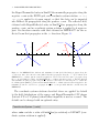
computations in 2D.
The propagation direction of the planewave is along the wavevector k =
(kx , ky , kz ), specified by the angles θ and φ, Figure 7. The angle theta
(θ ∈ [0◦ , 180◦ ]) is defined with respect to the negative kz component, for
the planewave propagating along the negative z-direction. The angle φ ∈
[0◦ , 360◦ ] is measured with respect to the positive direction of the x-axis.
Specification of the angle φ is optional, when omitted its value defaults to
π/2.
Two orthogonal polarizations of the planewave can be specified by setting
the polarization angle to 0◦ (E-field in the plane defined by the k and kz ) or
90◦ (E-field normal to the plane defined by the k and kz vectors). Specification of the polarization angle is optional, when omitted its value defaults to
0◦ .
In 2D computations only the angle θ ∈ [−90◦ , 90◦ ] has an effect, since the
wavevector is in the Y Z-plane, k = (0, ky , kz ), and hence φ = π/2, while the
polarization angle is determined by the Mode parameter: [Hx Ey Ez] mode
corresponds to 0◦ polarization angle, and [Ex Hy Hz] mode – to the 90◦ .
The planewave source can be used together with the PML, periodic or
Floquet boundary conditions, also known as Bloch periodic boundary conditions. The PML and periodic boundary conditions can be combined for
different axis, as described below. The Floquet boundary condition is appropriate for simulating periodic structures, and always implies PML boundaries
along the z-axis and Floquet boundary conditions along the x- and y-axis.
The planewave source is implemented using the Total Field/Scattered
Field (TFSF) formulation, with the TFSF boundaries defined two points
away from the PML absorbing boundary. The TFSF boundary consists of
6 planes (4 line segments in 2D) that make up a surface of a cube in 3D (a
4
PARAMETER FILE DESCRIPTION
28
z
o
E (0 )
o
E (90 )
kz
θ
k
y
φ
ky
x
kx
Figure 7: Definition of the parameters for the planewave source. Incidence direction k is specified by the
angles θ and φ, while the polarization angle can be set to the one of the two orthogonal directions: in the
plane, or orthogonal to the plane defined by the kz and k vectors.
rectangle in 2D) (Figures 8-9) and provide the means to truncate in space
the infinitely extended planewave. Figure 8 shows the Y Z-cross-section of
the computational domain, with an example of a planewave that propagates
in the negative z- and positive y-direction.
When a periodic boundary condition is specified for any of the axis, then
there will be no TFSF-boundary plane normal to that axis, Figure 9 . For
example, if periodic boundary conditions are used for the x and y-axis, the
only relevant TFSF boundaries are the top and bottom XY -planes. When
a periodic boundary condition is set for some axis w ∈ x, y, z, then in order
for the planewave to be a valid solution, the domain size Lw along the waxis and the planewave wavevector kw (θ, φ) must satisfy the condition Lw =
n × 2π/kw , where n = 1, 2, ....
The TFSF-boundary entry in the planewave specification is optional. It
can be used in conjunction with the periodic boundary conditions for the x
and y-axes to specify that only the top TFSF-boundary XY -plane should
be used for a planewave source, as is the case in Figure 9 (right).
In the TFSF formulation, the planewave source is applied at the TFSF
boundary, and the planewave propagates only in the Total Field region. Outside of the TFSF boundary only the Scattered Field is present. Simulations
that use TFSF formulation for the planewave source, must have a refractive
4
PARAMETER FILE DESCRIPTION
29
zmax
PML
TFSF boundary
Total Field =
Incident planewave
y
ymin
Scattered Field
Scattered Field
z
zmin
+
PML
+θ
Scattered Field
Scattered Field
PML
Scattered Field
PML
ymax
Figure 8: YZ-cross-section of the computational domain with Total Field/Scattered Field (TFSF) formulation for the planewave source. The refractive index must be the same at all sides of the TFSF boundary.
index distribution in the computational domain, such that the refractive index nref is same at all TFSF boundaries. Hence, the TFSF planewave source
is appropriate for problems that involve interaction of a planewave with isolated (or periodic) objects embedded in a uniform medium, for example,
scattering of a planewave from a chain of metallic nanospheres embedded in
a glass substrate.
The Floquet boundary condition allows simulation of a planewave incident
at an arbitrary angle on a structure that is periodic along the x- and/or yaxis. With this boundary condition the Lx and Ly can be arbitrary and do
not have to be integer multiples of 2π/kx , 2π/ky . Therefore a single unit cell
of the periodic structure can be modeled.
4
PARAMETER FILE DESCRIPTION
30
PML
PML
Periodic
Periodic
PlaneWave source TFSF top z­plane, or DIFFRACT source plane)
TFSF area
z
Periodic
y PML
x
Periodic
Scattering Object
PML
Scattering object
Figure 9: Left: computational domain with PML boundaries along all axis and Total Field/Scattered Field
(TFSF) formulation for the planewave source. The scattering object is enclosed by the TFSF surface, the
refractive index must be the same at all sides of the TFSF boundary. Right: computational domain with
PML boundaries along the z-axis, and periodic (or Floquet) boundary conditions along the x- and y-axis.
It is assumed in this plot that the TFSF-boundary [top] option is in effect for the planewave source.
4.17
Gaussian beam source specification
One or more gaussian beams can be specified for 2D or 3D computations by
using a GaussianBeamSource:
GaussianBeamSource:
Wavelength
Mode
Exyz-component
FWHM
beam-waist-offset
direction
phase
x0,y0,z0
xmin,xmax
ymin,ymax
zmin,zmax
[micron]
[Hx_Ey_Ez]
[y]
[micron]
[micron]
[plus/minus]
[degrees]
[micron]
[micron]
[micron]
[micron]
0.633
2.0 2.0
0.0
1
90.0
0.0 0.1 0.0
0.0 0.0
-5.0 4.0
0.2 0.2
The Mode can be [Hx Ey Ez],[Ex Hy Hz] or [3D]. For the [Hx Ey Ez] mode,
the polarization component can be set to [y] (for propagation along z) or
[z] (for propagation along y). For the [Ex Hy Hz] mode, polarization is
[x], and for 3D computations it can be [x] or [y]. In 2D computations (in
the Y Z-plane) the beam propagates by default along the positive direction
of the y or z-axis. In 2D the line segment, along which the source is ap-
4
PARAMETER FILE DESCRIPTION
31
plied, is specified by the ymin,ymax and zmin,zmax options, and xmin,xmax
is ignored. Only one of the ymin,ymax or zmin,zmax pairs can have distinct
values, hence specifying a line segment aligned with the y or z-axis. In the
example above the source is applied from y = −5µm to y = +4µm along the
y-axis, at z = 0.2, as specified by zmin,zmax. The x0,y0,z0 specifies the
beam center. In 2D only y0 or z0 is used to set the beam center position.
The FWHM specifies two numbers (in micron) for the amplitude full-width
half-max of the beam width at z = 0. For the 3D case √
the amplitude FWHM
values are related to w0x and w0y by FWHM=w0x/y 2 ln 2. In 2D case w0x
and w0y must√be set to the same number and represent an amplitude FWHM
equal to w0 2 ln 2. The w0 , w0x , w0y correspond to the formulas described
below. The parameter beam-waist-offset sets an initial shift of the beamwaist plane from the source plane, and corresponds to the variable z in
equations (1)-(3). The parameter direction is optional. It sets the direction of propagation along (+1) or against (-1) the positive direction of the
y or z-axis in 2D (Figure 10), and along or against the positive direction of
the z-axis in 3D. The default propagation direction is +1 in 2D computations.
GaussianBeamSource:
Wavelength
Mode
[3D]
Exyz-component
FWHM
beam-waist-offset
x0,y0,z0
xmin,xmax
ymin,ymax
zmin,zmax
[micron]
[y]
[micron]
[micron]
[micron]
[micron]
[micron]
[micron]
0.633
1.5
0.0
0.0
-7.0
-7.0
0.4
1.5
0.0 0.0
7.0
7.0
0.4
In 3D computations the beam propagates by default along the z-axis in
the negative direction, similar to the DiffractSource.
The phase parameter is also optional. It specifies the constant phase shift
φ0 to be added to the time harmonic dependence of the beam source, ωt+φ0 .
The default value of the phase shift is zero.
The default propagation direction can be changed as discussed above. In
3D only x0,y0 is used to set beam center, and zmin,zmax must both be
equal and set to the desired location of the source plane along the z-axis.
4
PARAMETER FILE DESCRIPTION
32
The source is computed according to the following formula, E(x, y, z, t) =
ŝ exp [i(kz − ωt)]Ê, with complex-valued Ê envelope given in 3D by:
2
2
Ê(x, y, z) = f (z)e−i[φx (z)+φy (z)]/2 e−x /wx (z)−y
2
2
× eik[x /(2Rx (z))+y /(2Ry (z))] ,
2
/wy2 (z)
×
(1)
q
where f (z) = w0x w0y /[wx (z)wy (z)], and
φx (z) = atan
z
!
lDx

2 
, wx2 (z) = w0x
1+
z
lDx
!2 
,

lDx
Rx (z) = z 1 +
z
!2 

(2)
lDx =
and similar definitions apply to functions with y-label. In 2D
(∂ Ê/∂x ≡ 0) the corresponding formulas are:
2
πw0x
/λ,
2
Ê(y, z) = f (z)e−iφ(z)/2 e−ρ
/w2 (z) ikρ2 /(2R(z))
e
,
(3)
q
f (z) = w0 /w(z), ρ2 = y 2 or ρ2 = z 2 , and

z
z
φ(z) = atan
, w2 (z) = w02 1 +
lD
lD
!
!2 
,

lD
R(z) = z 1 +
z
!2 

(4)
and lD = πw02 /λ. In the equations, k is the wavenumber in the incidence
medium, and λ is the wavelength in the incidence medium. The unit vector
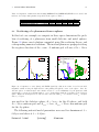
Figure 10: Ey and Ez components of a 2D Gaussian beam sourced along the y-axis at zmin = zmax = 3.5µm
with beam amplitude FWHM= 0.5µm, λ0 = 0.65µm, nref = 1.3, and direction set to -1. The z-parameter
is +4µm, resulting (for a beam that propagates in the −z direction), in initial focusing.
along the linear polarization direction is denoted by ŝ. Formulas (1)-(3)
4
PARAMETER FILE DESCRIPTION
33
Figure 11: Ey and Sy components of a 3D Gaussian beam.
assume that z-axis is the direction of propagation, and are an exact solution
to the Schrödinger equation,
∇2 Ê(x) = −2ik
∂ Ê(x)
∂z
(5)
2
Ê(x)
is small.
derived from Maxwell’s equations, assuming that ∂ ∂z
2
In the case of multiple beam sources, GaussianBeamSource: entries in
the parameter file must be specified one after another.
4.18
2D source specification from the file
One or more arbitrary source distributions can be specified as a file input
for two-dimensional computations. Example:
UserSource:
Wavelength
Mode
Filename
ymin,ymax
zmin,zmax
[micron]
[Hx_Ey_Ez]
[string]
[micron]
[micron]
0.9
usersource.dat
-1.5 1.5
1.0 1.0
Parameter Mode can be either [Hx Ey Ez] for a (Hx , Ey , Ez ) 2D mode or
4
PARAMETER FILE DESCRIPTION
34
[Ex Hy Hz] for (Ex , Hy , Hz ) mode. The ymin,ymax, zmin,zmax specify the
extent of the source. The source is applied along the y or z aligned coordinate
lines, so either ymin,ymax or zmin,zmax must be equal.
The ASCII text file is expected to contain on the first line the number
of points present in the file. The following lines must contain 5 columns:
coordinate of the point in microns, real part of Field1, imaginary part of
Field1, real part of Field2, imaginary part of Field2. The fields Field1 and
Field2 are defined as:
for [Hx Ey Ez] mode
Field1 is Hx
Field2 is Ez , if ymin equals ymax, or
Field2 is Ey , if zmin equals zmax,
for [Ex Hy Hz] mode
Field1 is Ex
Field2 is Hz if ymin equals ymax, or
Field2 is Hy , if zmin equals zmax.
The range of coordinates of the source points in the file may be a subset
or superset of the range specified by ymin,ymax or zmin,zmax. The complex
valued field amplitudes are read and interpolated into the FDTD grid. The
interpolated values are written to an output file with the same name as the
input source file plus a “.interpN” extension, where N is the rank of the
processor that created the file. The content of the “.interpN” file is the same
as that of the input source file, with two exceptions: the first line specifying
the number of points is omitted, and there is an additional field (last entry)
on each line, identifying material logical index along the source line.
The E and H-fields are sourced in time with time-harmonic ansatz e−iωt
as Re[Hx (y, z)e−iωt ], Re[Ey (y, z)e−iωt ], etc. Appendix C Figure 38 gives a
detailed description of the required staggered E and H field positioning of the
user-defined source for the 2D Hx Ey Ez and Ex Hy Hz computations. In the
case of multiple user defined sources, UserSource entries in the parameter
file must be specified one after another.
4
PARAMETER FILE DESCRIPTION
35
0.8
(ymax,zmax)
0.6
0.4
0
-0.2
n3
source line segment
z [µm]
0.2
n2
waveguide center
n1
waveguide width
-0.4
-0.6
-0.8
-1
(ymin,zmin)
-0.8
-0.6
-0.4
-0.2
0
y [µm]
0.2
0.4
0.6
0.8
1
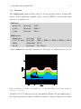
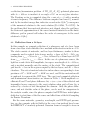
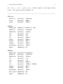
Figure 12: Example of a waveguide running along the y-axis, with the source applied on a line-segment along
the z-axis, at ymin = ymax = −0.8µm. The refractive index distribution, waveguide width and center-line
position are specified as part of the WaveguideSource definition, and should correspond to the geometry
and material properties specified in the geometry and material definition files.
4.19
2D planar waveguide source specification
A planar waveguide source for Ex Hy Hz or Hx Ey Ez mode is specified by
its effective index n eff = β/k, where β is a mode propagation constant,
and k = 2π/λ is a free space wavenumber. The refractive index is n2 for
the waveguide, and n1, n3 for the cladding layers. The position of the center
and width of the waveguide, and refractive index values n1,n2,n3 must correspond to the structure and material properties specified in the geometry
and material definition files. The sourced mode has a wavevector along the
positive direction of the y- or z-axis.
4
PARAMETER FILE DESCRIPTION
36
WaveguideSource:
Wavelength [micron]
0.65
Mode
[Hx_Ey_Ez]
ModeNumber
0
n_eff,n1,n2,n3
1.49797 1.0 1.75 1.0
center,width [micron]
3.0 0.3
ymin,ymax [micron]
0.0 6.0
zmin,zmax [micron]
0.3 0.3
The ymin,ymax, zmin,zmax specify the extent of the source. The source
is applied along the y or z aligned coordinate lines, so either zmin,zmax or
ymin,ymax must be equal, Figure 12. For example, for a waveguide running along the z-axis, the waveguide mode is sourced across the waveguide
along the y-axis, so zmin must be equal to zmax and equal to the desired zlocation of the source line. The range of ymin,ymax should be large enough
to cover the regions where the source field amplitudes are not negligible.
If the ymin,ymax,zmin,zmax extend outside of the computational domain,
they are reset to the edge of the computational domain or PML region.
4.20
File format version compatibility with DIFFRACTTM
This entry is optional in the input file. It specifies the version of DIFFRACTTM
software with which the DiffractSource and export files should be compatible:
ExportFileFormat [version] 8.2
The export files are produced by the “ExportReflected” and “ExportTransmitted” entries described in subsections 4.22.1-4.22.2.
If the file format version is not specified, the default is compatibility with
DIFFRACTTM versions 8.4 and up. When using source files (subsection
4.14) created with DIFFRACTTM versions 8.3 and lower, it is mandatory
to explicitly specify the file format version, otherwise the source distribution
will be incorrect. When DIFFRACTTM source file is used, the ExportFileFormat is set to the same format as the source. The different file formats
are as follows:
For DIFFRACTTM versions less than 8.2:
4
PARAMETER FILE DESCRIPTION
37
the file contains on the first line the refractive index nr (assumed to be
constant in the sampling plane), followed on the second line by Nx , Ny , Lx , Ly
and complex-valued field distributions Ex (x, y), Ey (x, y), Ez (x, y), followed
by δ and Hx (x, y), Hy (x, y), Hz (x, y). The fields are sampled on a uniform grid with steps Lx /Nx and Ly /Ny in x and y-directions. The variable
δ is equal to the FDTD grid cell size in a direction normal to the plane,
and at the position of the plane, on which E and H fields are sampled.
Negative values of δ specify that Hx (x, y), Hy (x, y) fields are sampled on a
plane located along the z-axis a distance of |δ|/2 behind the plane on which
Ex (x, y), Ey (x, y) fields are sampled (Figure 6), while positive δ corresponds
to H-fields sampled on a plane δ/2 ahead of the E-field plane. The δ and
domain sizes Lx ,Ly are in units of λ/nr . The E and H fields are in normalized units defined in the DIFFRACTTM manual. For a beam propagating in
DIFFRACTTM along the positive direction of the z-axis, the H-fields must
be sampled half a cell behind E-fields, hence negative δ = −∆z must be
specified in the FDTD/Export option of DIFFRACTTM when creating a file
for DIFFRACTTM source option described in section 4.14.
For DIFFRACTTM versions 8.2 and 8.3:
the file contains on the first line the refractive index nr , the wavelength in
the vacuum λ, the units of the wavelength (cm,mm,um,nm), followed on the
second line by Nx , Ny , Lx , Ly and the field distributions with intervening δ
as above. The domain sizes Lx and Ly , and δ are in units of the wavelength
λ in the vacuum.
For DIFFRACTTM versions 8.4 and above (default):
the same as the format of versions 8.2 and 8.3, but the E and H fields are
in physical units of V/m and A/m.
4.21
Coordinate system transformation
In Diffract the beam nominally propagates along the positive z-axis. In
Sim3D Max the incident DiffractSource beam cross-section is intended for
propagation along the negative z-axis, Figure 13. Hence, a coordinate transformation z → −z, y → −y is applied to the E(x, y) and H(x, y) fields read
from the Diffract source file. Similarly, the transmitted field obtained with
4
PARAMETER FILE DESCRIPTION
38
the ExportTransmitted entry in Sim3D Max nominally propagates along the
negative z-axis in the FDTD grid, and coordinate system rotation −z → z,
−y → y is applied to it upon export, so that the data can be imported
into Diffract for propagation along the positive z-axis. The reflected field,
obtained with ExportReflected entry in Sim3D Max, propagates along the
positive z-axis, and no coordinate system rotation is applied to it upon export. Its direction coincides with that obtained in DIFFRACT for the reflected beam that propagates in the +z direction, Figure 13.
1
DIFFRACT
Z
1
Sim3D_Max
Z
I
T
R(-y,-z)
0.5
R
0.5
T(-y,-z)
0
-1
R
0
0
-0.5
-0.5
0.5
I
-1
1
Y
-1
0
-0.5
-0.5
0.5
T
-1
Figure 13: In DIFFRACT the incident and transmitted beams (solid blue lines) propagate along the
+z direction, hence the reflected beam (dashed blue line) propagates along the −z. Upon reflection, in
DIFFRACT a coordinate system rotation is applied in order for the reflected beam to propagate along
the +z as well (dashed red line). In Sim3D Max the coordinate system is rotated, so that the incident
and transmitted beams propagate along the −z direction, and reflected beam along the +z. When the
CoordinateSystem [Diffract] option is used in Sim3D Max, the coordinate system rotation is applied to the
transmitted beam, in order for it to propagate along the +z, in agreement with the convention used in
DIFFRACT.
The coordinate system rotations described above are applied by default
to the field distributions of the source and ExportTransmitted XY -planes
(but not XZ or Y Z-planes) when Diffract input file is used as a source. The
default can be changed with an optional entry:
CoordinateSystem [code]
where code can take a value of Sim3d Max (no rotation) or DIFFRACT (coordinate system rotation is applied).
1
Y
4
PARAMETER FILE DESCRIPTION
4.22
39
Export file specification
The spatial distribution of the amplitude and phase of the E and H fields on
a specified plane, and at the frequency of the source, can be obtained using
ExportReflected and ExportTransmitted entries. These objects can be used
with any source, and produce files in a format compatible with the FDTD
import/export interface of the DIFFRACTTM software.
The difference between ExportReflected and ExportTransmitted entries is
that the reflected field is sampled on the XY -plane at a predefined position,
while the ExportTransmitted can specify any coordinate plane with arbitrary
location. The ExportReflected plane will be positioned just above the source
plane, when used with a PlanewaveSource or DiffractSource at its default
location, so that only the reflected field is sampled.
Because of the possibility to arbitrarily place the source and the ExportTransmitted sampling planes, the meaning of “reflected” or “transmitted”
may be lost, depending on the relative location of the sampling plane positions and the source plane location.
4.22.1
Export of the reflected field
This item is optional in the input file. It can be used to obtain complexvalued distribution of the fields in the XY -plane. The specified output file
conforms to the file structure used in the FDTD import/export option of
DIFFRACTTM :
ExportReflected:
Filename
File Format
Grid Type
NX,NY
fdtd.export.reflected
ascii
collocated
256 256
The File Format can be one of ascii, fortran binary, c binary, and
Grid Type can be staggered or collocated as described in sub-section
4.14. A collocated grid and ASCII or Fortran binary format must be used
when generating files intended for input into DIFFRACTTM via FDTD Import option. The NX,NY option specifies the desired number of points along
the x and y axis. The line specifying NX,NY can be omitted. In that case the
number of points will be set to the Nx , Ny of the DIFFRACTTM input source
4
PARAMETER FILE DESCRIPTION
40
file 4.14, or, if another source is used, Nx , Ny are set to the number of points
in the XY -plane of the FDTD grid. The scattered field complex-valued amplitude is computed in the xy plane at z = zmax − (nz P M L + 2)∆ztop via the
Discrete Fourier Transform of the time dependent solution, applied in the
time interval [tmax − 4λ/c, tmax ]2 , where ∆ztop is the grid spacing used near
the PML region at the top of the computational domain. There can be only
one ExportReflected: entry in the input file, and its position on the grid is
always at the top of the domain as specified above, regardless of the position
along the z-axis of any of the sources. When used with DiffractSource or
PlanewaveSource at their default locations, the ExportReflected plane will
be just above the source plane and will sample only the reflected fields.
4.22.2
Export of the transmitted field
If ExportReflected: entry described above is specified, it must also be
followed by at least one "ExportTransmitted:" entry. This entry is similar
to the entry for the reflected field, but its plane has a user-defined, rather
than default, position. If an "ExportTransmitted:" entry is not necessary
in the computation, its position can be set to be outside of the computational
domain, and it will be ignored.
The ExportTransmitted: entry sets the filename of the export file into
which to write complex-valued amplitude distribution of the Ex , Ey , Ez and
Hx , Hy , Hz fields computed at the specified plane. The file content and parameters are the same as for the reflected field described above.
ExportTransmitted:
Filename
File Format
Grid Type
z-location [micron]
NX,NY
fdtd.export.transmitted
fortran_binary
collocated
-50e-3
512 512
In addition, z-location specifies the position of the plane along the zaxis, in micrometers. If this position is outside of the computational domain
bounds, no output file will be produced. The line z-location corresponds
to fields sampled in the XY -plane. Similarly, y-location or x-location
2 Note, that changing z
max will change the Diffract source and export reflected field plane positions. Also, tmax , is set
independently of zmax , and should be chosen large enough to get time-harmonic converged solution.
4
PARAMETER FILE DESCRIPTION
41
can be used to sample fields in the XZ or Y Z planes. The line specifying the
number of points in the sampling plane (NX,NY for the XY -plane, NX,NZ for
the XZ-plane, or NY,NZ for the Y Z-plane) can be omitted, in which case the
number of points will default to the values from the DIFFRACTTM source
file 4.14, or, if DIFFRACTTM source is not used, to the number of points in
the corresponding plane of the FDTD grid.
After the line specifying the number of points, an optional specification of
the sampling region can follow. For example in the Y Z-plane one can specify
an area centered on the point (0,0) as LY,LZ [micron] 2.4 1.0. When not
specified, the sampling region will be set to the computational domain size
for the corresponding cross-section. One exception is when DIFFRACTTM
source is used: then the sampling region in the XY -plane is set to Lx , Ly
values read from the DIFFRACTTM source file.
The reflected or transmitted field magnitude and phase data can be requested as follows:
magnitude,phase
magnitude,phase
Poynting vector
current density
Ex,Ey,Ez?
Hx,Hy,Hz?
Sx,Sy,Sz?
Jx,Jy,Jz?
yes
yes
yes
yes
yes
yes
yes
yes
yes
yes
yes
yes
All of the above lines are optional, and when omitted, or when set to “no”,
the corresponding output files are not generated. When specified, a folder is
created in the working directory into which the files are written under the
names “mEx.dat”, “mEy.dat”, etc. for the magnitude data, and “pEx.dat”,
“pEy.dat”, etc. for the phase data (in radians). For the real-valued Poynting vector only amplitude data “Sx.dat”, etc., is generated. The files are
written in a text (ASCII) format and in the same “xy” order as the data
in the export file. The magnitude and phase folder has the same name as
the export file, but without the filename extension. If the export filename
does not have an extension, a suffix “-mp” is added to it to create the folder
name.
There can be multiple “ExportTransmitted:” entries, specified one after
another, for sampling the computational domain with different planes and at
various locations. Note however, that when an export plane is at a location
such that it samples a region with refractive index variation in that plane,
then the refractive index value stored in the export file is not well defined,
4
PARAMETER FILE DESCRIPTION
42
since it will represent only one value of the refractive index distribution in
the export plane. In such cases magnitude and phase distributions of the exported fields are not suitable for propagation in the DIFFRACTTM software,
since it requires constant refractive index in the export plane. However, the
data can be visualized or processed otherwise.
4.23
Monitor header comment
A sequence of characters can be added at the beginning of the first line of
the Monitor files described in section 4.24. For example,
MonitorFileComment
[string]
#
will put # as the first character on the first line (which describes the monitor
type, number of points, etc.) in all Monitor files. This entry is optional in
the input file.
4.24
Monitor specification
Monitors are optional in the input file. They can be used to sample fields
at specified points and within a specified time interval. Parameter Mode
can be either [3D], [Hx Ey Ez] for a (Hx , Ey , Ez ) 2D mode or [Ex Hy Hz]
for (Ex , Hy , Hz ) 2D mode. The Type can be either [fourier-transform]
or [time-history]. The output file specified under Filename is an ASCII
text file.
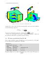
Monitor:
Mode
Type
Filename
xmin,xmax
ymin,ymax
zmin,zmax
t_on,t_off
bandwidth
fmin,fmax
[Hx_Ey_Ez]
[fourier-transform]
[string]
monitor1.out
[micron]
0.0 0.0
[micron]
-1.0 1.0
[micron]
0.0 0.0
[periods]
8
[frequency-interval]
[THz]
285.0 315.0
Another monitor example:
4
PARAMETER FILE DESCRIPTION
43
Monitor:
Mode
[Ex_Hy_Hz]
Type
[time-history]
Filename
[string]
monitor2.out
xmin,xmax [micron]
0.0 0.0
ymin,ymax [micron]
-1.0 1.0
zmin,zmax [micron]
0.0 0.0
t_on,t_off [nanoseconds] 10e-6 20e-6
sampling-factor [integer] 5
During parallel computation with Np CPUs, each processor writes to its own
output file, so processor rank (an integer number, between 0 and Np − 1) is
appended to the output filename, e.g. monitor1.out3. The content of the
output file depends on the Mode entry, and is described below. With each
new simulation, the existing monitor files with the same name as specified
under the Filename (with appended processor numbers), are removed.
The xmin,xmax, ymin,ymax, zmin,zmax specify the extent of the monitor. The t on,t off sets the monitor switch-on and switch-off times, and
can be specified either as
t_on,t_off [nanoseconds]
10e-6 20e-6
or
t_on,t_off [periods]
10
In the case when number of [periods] P is specified, the sampling in time
is done from tmax − P × T to tmax , where T = λ/c is the period of the source.
For the [fourier-transform] monitor, the bandwidth entry must be
present with one of the options:
bandwidth [source-frequency], bandwidth [frequency-interval] or
bandwidth [wavelength-interval].
The first option, [source-frequency], specifies that Fourier Transform
should be evaluated at a single point in the frequency space - the input source
frequency.
The [frequency-interval] (or [wavelength-interval]) option allows
Fourier Transform to be computed for a range of frequencies (or wavelengths), specified on the next line with an entry fmin,fmax (or lmin,lmax),
4
PARAMETER FILE DESCRIPTION
44
for example: fmin,fmax [THz] 285.0 315.0 or lmin,lmax [nm] 850.0
920.0.
The sampling-factor specification is optional. It can be used to set the
decimation factor for sampling fields in time. For example sampling-factor
[integer] 5 sets monitor data processing to occur only every 5th time step.
The default sampling factor is 1.
The output of the monitor of time-history of fields on a specified area
(which also generates time history of the area integral of the Poynting vector
component Sn normal to the plane) can be controlled by specifying on the
last line of the monitor entry whether to create files with time-history of
E,H and S (output [distribution]) or only time-history of the integral
of Sn (output [integral]), or both (output [all]). When output type is
not specified, the default is output [all].
4.24.1
Monitors for computations in 2D
For T Ex /T Mx computations in 2D, the xmin,xmax values are ignored, and
only one of the ymin,ymax or zmin,zmax pairs must have distinct min/max
values. The monitor then specifies a line segment aligned with the y or zaxis. Along this line either the time history or Discrete Fourier Transform of
the E, H fields and the Poynting vector S = E × H are sampled and written
to the specified file.
For a [time-history] monitor, the output file contains on the first line
the computation mode, monitor type, number of monitor points in space and
number of points sampled in time, e.g. [Ex Hy Hz] [time-history] Ny Nz
Ntime.
The rest of the file consists of one line for each point in space and time
with the following 8 columns: time in nanoseconds, y,z-coordinates of the
point in microns, Field1, Field2, Field3, Field4, Field5. The fields Field1
through Field5 are defined as:
for [Hx Ey Ez] mode
Field1 is Hx , Field2 is Ey , Field3 is Ez ,
Field4 is Sy , Field5 is Sz ,
for [Ex Hy Hz] mode
4
PARAMETER FILE DESCRIPTION
45
Field1 is Ex , Field2 is Hy , Field3 is Hz ,
Field4 is Sy , Field5 is Sz .
For a [fourier-transform] monitor, the file contains on the first line
the computation mode, monitor type, number of monitor points in space
and number of points sampled in frequency, e.g.
[Ex Hy Hz] [fourier-transform] Ny Nz Nfreq.
If bandwidth [source-frequency] option was selected, the Nfreq will be
equal to 1.
The rest of the file consists of one line for each point in space and frequency
with the following 11 columns: frequency value in THz, y,z-coordinates of
the point in microns, Field1, Field2, Field3, Field4, Field5, Field6, Field7,
Field8. The fields Field1 through Field8 are defined as:
for [Hx Ey Ez] mode
Field1, Field2 are Re(Hx ), Im(Hx ),
Field3, Field4 are Re(Ey ), Im(Ey ),
Field5, Field6 are Re(Ez ), Im(Ez ),
Field7 is real < Sy >, Field8 is real < Sz >,
for [Ex Hy Hz] mode
Field1, Field2 are Re(Ex ), Im(Ex ),
Field3, Field4 are Re(Hy ), Im(Hy ),
Field5, Field6 are Re(Hz ), Im(Hz ),
Field7 is real < Sy >, Field8 is real < Sz >.
The complex valued amplitudes of the E and H fields are computed via
time Discrete Fourier Transform of the real valued E and H FDTD variables. The DFT is evaluated at the source frequency if bandwidth option
is set to [source-frequency]. The real valued components of the time averaged Poynting vector are computed from complex valued E and H fields,
as < S > = 21 Re(E × H∗ ). This formula assumes a continuous wave timeharmonic dependence of fields.
5
BOUNDARY CONDITIONS FILE DESCRIPTION
4.24.2
46
Monitors for computations in 3D
For 3D computations, parameter Mode is set to [3D], and xmin,xmax,
ymin,ymax or zmin,zmax can be used to specify a line segment or a plane
section along which the monitor is applied. For a line segment, only one
of the min/max coordinate pairs can have distinct values, so that the line
segment is aligned with one of the x,y or z-coordinate directions. For a plane
section, only two of the min/max coordinate pairs can have distinct values,
so that the section is in the XY , Y Z or XZ plane.
In 3D, for a monitor type [time-history], the first line specifies the 3D
computation mode, monitor type, number of monitor points in space and
number of points sampled in time, e.g. [3D] [time-history] Nx Ny Nz
Ntime. The output file contains one line for each point in space and time
with the following 13 columns: time in nanoseconds, x,y,z-coordinates of the
point in microns, Ex,Ey,Ez, Hx,Hy,Hz, Sx,Sy,Sz.
For a 3D [fourier-transform] monitor, the output file contains one line
for each point in space with the following 19 columns: frequency value in
THz, x,y,z-coordinates of the point in microns, Re(Ex), Im(Ex), Re(Ey),
Im(Ey), Re(Ez), Im(Ez), Re(Hx), Im(Hx), Re(Hy), Im(Hy), Re(Hz),
Im(Hz), Sx, Sy, Sz.
For a plane monitor in 3D, an additional file is generated, containing the
area integral of the Poynting vector component normal to the plane as a
function of time or frequency. The filename of this file is the same as that of
the monitor file, but with extension “.is” added before the processor rank.
An integral of the electromagnetic energy (E·D+H·B)/2 over a specified
volume containing only dielectric materials, can be monitored as a function
of time with an [energy] monitor. A volume is specified with all min/max
coordinate pairs having distinct values. Detailed summary of the monitor
file formats is given in Appendix D.
There can be multiple “Monitor:” entries in the parameter file, specified
one after another.
5
Boundary Conditions File Description
The file specified under the Boundary Conditions Filename: entry of the
parameter file (see 4), contains a definition of the BCs used in the simulation.
5
BOUNDARY CONDITIONS FILE DESCRIPTION
47
Currently, boundary types [PEC], [periodic], [Floquet] or [PML] can
be used. The selected boundary condition applies to both top and bottom
boundaries of the specified axis.
• The Perfect Electric Conductor (PEC) boundary condition sets
the tangential electric field components to zero on the boundary.
• The periodic boundary condition allows simulation of the periodic
systems in 2D or 3D.
• The Floquet boundary condition is used with the planewave source
(sec. 4.16) to model periodic systems in 2D or 3D, with arbitrary
planewave incidence angles.
• The Perfectly Matched Layer (PML) option sets up an absorbing
layer that simulates an open boundary condition.
An example of the content of the boundary conditions file, that sets the
x-axis to a 15 point PML with default PML parameters for σ and κ, y-axis
to periodic and z-axis to PEC:
BoundaryConditions:
x-axis
[PML]
nz_pml
15
sigma,kappa
0.0 0.0
y-axis
[periodic]
z-axis
[PEC]
If the desired boundary type is PML for any of the axes, the next line
after ...-axis [PML] must specify for that axis the number of points in
the absorbing layer, followed by sigma,kappa - the values of σmax and κmax
at the end of the absorbing layer. A polynomial of order mpml = 3 is used
in computing the grading of the PML layers. If σmax or κmax are set to
zero, they will assume their respective
default values of κmax = 1.0 and
q
σmax = 8 × (mpml + 1)/(npml ∆ µ0 /0 ), where ∆ is the cell size in the PML
region. Inside the PML layers the material refractive index and grid cell sizes
should not have any variation in the direction normal to the PML layer.
If the boundary specification file is empty, the default boundary condition
is PML absorbing boundary for all axes, with a default number of points
in the PML layers set to nx,y P M L = 10 and nz P M L = 15. This results in
6
MATERIAL FILE DESCRIPTION
48
approximately -40 db reflection for dielectric media. The default settings
can be modified using a specification of the boundary type for each axis.
The Floquet boundary condition, used with the planewave source, can be
set with an entry x-axis [Floquet] or y-axis [Floquet] for the x- or
y-axis.
6
Material File Description
The file specified under the Material Definition Filename: entry of the
parameter file (see 4), contains a definition of the material properties used
in the simulation. The file can contain an arbitrary number of material definitions. Each material can be of one of the predefined types: dielectric,
dielectric(x,y), Debye, Lorentz, etc. Each material declaration starts
with two lines:
Material Label
model
[string]
YourLabel
[MaterialType]
where YourLabel is a unique arbitrary word (except for the reserved word
Vacuum) chosen by the user to identify each material. The material label
Vacuum is predefined as a dielectric with permittivity 0 and permeability µ0 .
Material Type is one of the available types: dielectric, Debye, Lorentz,
etc. For example,
Material Label
model
[string]
[dielectric]
SiO2
Material Label
model
[string]
[Debye]
Gold
Material Label
model
[string]
[Lorentz]
AluminumOxide
These two lines are followed by a set of parameters specific to the material type.
6
MATERIAL FILE DESCRIPTION
6.1
49
Dielectric materials
For the type dielectric, the material properties can be entered in any one
of the following equivalent formats:
Material Label
model
sqrt Re(eps)
conductivity
Material Label
model
n-ki
Material Label
model
eps
[string]
GaAs750nm
[dielectric]
[dimensionless] 3.6986
[1/(ohm*m)]
16455.9
[string]
GaAs750nm
[dielectric]
[dimensionless] 3.7-0.1i
[string]
[dielectric]
[relative]
GaAs750nm
13.68-0.74i
When used with a monochromatic source, materials with a complex refractive
index n − ki can be modeled by the material type dielectric if n2 − k 2 > 1
(in the case of arbitrary n and k refer to the Debye material model). The
refractive index n − ki,qpermittivity
√ and conductivity σ are related by
2
= r + ii = (n − ki) , Re() = n2 − k 2 and σ = 2nk0 ω, where ω is the
frequency of the source.
Arbitrary continuous variation of the refractive index and conductivity in
the XY -plane can be realized with material model dielectric(x,y). This
model is useful for simulating optical disk data storage components in which
optical constants are continuous functions of the temperature in the plane
of the disk, T = T (x, y). For the material type dielectric(x,y), there is
one input parameter: the name of the file with the distribution of the optical
constants, e.g.
Material Label
model
filename
[string]
[dielectric(x,y)]
[string]
GST
GST.input
The data file is an ASCII file containing on the first line a single word,
e.g. Dielectric(x,y), followed on the second line by:
Lxmin Lxmax Lymin Lymax N x N y (nbg σbg )
6
MATERIAL FILE DESCRIPTION
50
where Lxmin , Lxmax , ... specify the domain size (in nanometers) in which
the data is defined, N x, N y are the number of rows, columns in the file, and
(nbg σbg ) are the background refractive index and conductivity. Subsequent
lines must contain entries (nij σij ) for each point i, j of the grid defined on
the first line. The units of n and σ must be the same as in the material
model [dielectric] described above. The data in the file is read in the
order indicated by the following pseudo-code segment:
for i=1 to Nx
for j=1 to Ny
read (n[i][j] sigma[i][j])
Then the data is interpolated to the FDTD computational grid. The grid
points that are outside of the range specified by Lxmin , Lxmax , Lymin , Lymax ,
are assigned background optical constant values (nbg σbg ).
A more general distribution of the refractive index and conductivity, dependent on all of the coordinates, can be realized with the material model
dielectric(x,y,z).
Material Label
model
filename
[string]
GST-T
[dielectric(x,y,z)]
[string]
epsxyz.dat
The input data file is an ASCII file containing on the first line a single word,
for example Dielectric(x,y,z), followed by nx × ny × nz entries (nijk σijk )
for each point i, j, k of the grid defined in section 4.3. The data is read from
the file in the following order:
for i=1 to nx
for j=1 to ny
for k=1 to nz
read (n[i][j][k] sigma[i][j][k])
6.2
Debye model
The parameters for a dispersive medium based on the single-pole Debye
model correspond to a complex-valued frequency-domain susceptibility func-
6
MATERIAL FILE DESCRIPTION
51
tion χ(ω) and permittivity function (ω):
χ(ω) =
∆
,
1 + iωτ
(ω) = ∞ + χ(ω) − i
σ
ω0
(6)
with τ - the pole relaxation time, ∞ - the relative permittivity at infinite
frequency, ∆ = s − ∞ , where s is the static or zero-frequency relative
permittivity. An example set of parameters for gold (n = 0.16 − 3.95i) at
λ = 700nm:
Material Label
model
tau
eps_inf
delta_eps
conductivity
[string]
[Debye]
[femtosec]
[relative]
[relative]
[1/(ohm*m)]
Gold
4.84371
1.0
-2832.73
5.17818e6
The Debye model can be used to simulate materials which have a dispersion
relation that can be approximated by the expression (6) over some frequency
band.
The Debye model can also be used to represent materials with complexvalued refractive index n − ki at a specified frequency. In such cases, given
two parameters, n and k, the choice of four Debye model parameters is not
unique, Figure 14. At any given frequency ω the real and imaginary parts
4
4
0
0
-4
-4
-8
Re[ε(λ)]
Im[ε(λ)]
n(λ)
κ(λ)
-8
-12
-12
-16
-16
200
300
400
500
600
λ [nm]
700
800
900
1000
200
Re[ε(λ)]
Im[ε(λ)]
n(λ)
κ(λ)
300
400
500
600
λ [nm]
700
800
900
Figure 14: Dependence of complex-valued permittivity and refractive index on the wavelength λ = 2πc/ω
computed using single-pole Debye model (6) with two sets of model parameters for gold (n = 0.16 − 3.95i)
at λ = 700nm.
1000
6
MATERIAL FILE DESCRIPTION
52
of the equation = (n − ki)2 provide two conditions for the choice of Debye
parameters:
∆
,
1 + ω2τ 2
∆ωτ
σ
−2nk = −
−
,
1 + ω 2 τ 2 ω0
n 2 − k 2 = ∞ +
which can be rewritten in the following form:
∆ = (1 + ω 2 τ 2 )(n2 − k 2 − ∞ ),
σ
= −ωτ (n2 − k 2 − ∞ ),
−2nk +
ω0
(7)
(8)
By setting ∞ = 1, parameters σ and τ are determined by equation (8), linear
in both unknowns, with ∆ following from equation (7). The Debye model
corresponding to a given permittivity at source frequency can be realized by
specifying n − ki or in the material definition file, for example:
Material Label
model
n-ki
[string]
Aluminum
[Debye]
[dimensionless] 2-7i
Material Label
model
eps
[string]
[Debye]
[relative]
Gold
-15.0-1.2i
A multi-pole Debye model corresponding to the relative permittivity
(ω) = ∞ +
Np
X
∆p
σ
−j
ω0
p=1 1 + jωτp
can be set by specifying the number of poles Np , followed by the list of parameters for each pole, in the format shown below:
6
MATERIAL FILE DESCRIPTION
Material Label
model
poles
eps_inf
conductivity
tau0
delta_eps0
tau1
delta_eps1
53
[string]
M1
[multipole-Debye]
[integer]
2
[relative]
...
[1/(ohm*m)]
...
[femtosec]
...
[relative]
...
[femtosec]
[relative]
...
...
Similarly to the dielectric material model, arbitrary continuous variation
of the single-pole Debye model parameters in the XY -plane can be realized
with material type Debye(x,y). This model may be used, for example, to
simulate optical disk data storage components in which material parameters are continuous functions of the temperature in the plane of the disk,
T = T (x, y). For the material type Debye(x,y), there is one input parameter: the name of the file with the distribution of Debye model parameters, e.g.
Material Label
model
filename
[string]
[Debye(x,y)]
[string]
PtOx
PtOx.input
The data file is an ASCII file containing on the first line a single word,
e.g. Debye, followed on the second line by:
Lxmin Lxmax Lymin Lymax N x N y (τbg ∞ bg ∆bg σbg )
where Lxmin , Lxmax , ... specify the domain size (in nanometers) in which
the data is defined, N x, N y are the number of rows, columns in the file, and
the rest specify background Debye model parameters. Subsequent lines must
contain entries (τij ∞ ij ∆ij σij ) for each point i, j of the grid defined on
the first line. The units of parameters must be the same as in the material
model [Debye] described above.
The data is read from the file in the same order as for the dielectric(x,y)
material described above, and interpolated to the FDTD computational grid.
The grid points that are outside of the range specified by Lxmin , Lxmax ,
Lymin , Lymax , are assigned background values (τbg ∞ bg ∆bg σbg ).
6
MATERIAL FILE DESCRIPTION
6.3
54
Lorentz model
The parameters for a dispersive medium based on the single-pole Lorentz
model correspond to a complex-valued frequency-domain susceptibility function:
σ
∆ω02
,
(ω)
=
+
χ(ω)
−
j
χ(ω) = 2
∞
ω0 + 2jωδ − ω 2
ω0
where ω0 - is the pole frequency, ∞ - the relative permittivity at infinite frequency, ∆ = s − ∞ , s is the static or zero-frequency relative permittivity,
δ is the damping coefficient. Example parameters for aluminum (n = 2 − 7i)
at λ = 650nm:
Material Label
model
omega0
delta
eps_inf
delta_eps
conductivity
[string]
[Lorentz]
[rad/s]
[rad/s]
[relative]
[relative]
[1/(ohm*m)]
Aluminum
23.536118e14
2.9504974e14
1.81
32.802
0.0
Multi-pole Lorentz model corresponding to the relative permittivity
∆p ωp2
σ
= ∞ +
−
j
2
2
ω0
p=1 ωp + 2jωδp − ω
Np
X
can be set by specifying the number of poles Np , followed by ∞ and σ, and
the list of parameters for each pole, in the format shown below:
Material Label
model
poles
eps_inf
conductivity
[string]
M2
[multipole-Lorentz]
[integer]
2
[relative]
...
[1/(ohm*m)]
...
6
MATERIAL FILE DESCRIPTION
6.4
55
omega0
delta0
delta_eps0
[rad/s]
[rad/s]
[relative]
...
...
...
omega1
delta1
delta_eps1
[rad/s]
[rad/s]
[relative]
...
...
...
Drude model
The parameters for a dispersive medium based on the single-pole Drude
model correspond to a complex-valued frequency-domain susceptibility function:
ωp2
χ(ω) =
,
(ω) = ∞ + χ(ω)
2jωδ − ω 2
where ωp - is the plasma frequency, ∞ - the relative permittivity at infinite
frequency, δ is the damping coefficient. Example input parameters for Drude
model:
Material Label
model
delta
eps_inf
omega_p
6.5
[string]
[Drude]
[rad/s]
[relative]
[rad/s]
Metal
1e13
1.0
5e12
Magnetic material model
The [magnetic*] material type allows specification of magnetic permeability and electric permittivity for materials with constant µ 6= µ0 or with
magnetic dispersion. Example input parameters for constant and µ:
6
MATERIAL FILE DESCRIPTION
Material Label
model
permittivity
permeability
56
[string]
MagMat
[magnetic1]
[relative]
2.25
[relative]
2.0
Drude model is used to model electric and magnetic dispersion of magnetic
materials. Drude model parameters ∞ , δ, ωp can be specified instead of the
constant permittivity, resulting in (ω) frequency dependence given in subsection 6.4. Similarly, µ∞ , δm , ωm can be specified instead of the constant
permeability, with frequency dependent µ(ω) given by:
2
ωm
µ(ω) = µ∞ +
.
2jωδm − ω 2
Example input parameters for dispersive magnetic material:
Material Label
model
[string]
MetaMat
[magnetic2]
eps_inf
delta
omega_p
[relative]
1.0
[rad/s]
1.25e14
[rad/s]
8.0e15
mu_inf
delta_m
omega_m
[relative]
1.0
[rad/s]
2.5e14
[rad/s]
6.0e15
Debye(x,y), dielectric(x,y),dielectric(x,y,z) and magnetic material models currently can be used only in 3D computation mode,
and should not extend into PML layers.
7
GEOMETRY FILE DESCRIPTION
7
57
Geometry File Description
The file specified under the Geometry Definition Filename: entry of the
parameter file (see 4), contains definitions of the structures to be set up
in the computational domain. The default (i.e. empty geometry definition
file) is a free space computational domain occupied by the predefined material Vacuum, see section 6. More complex structures may be simulated by
adding any number of geometric objects to this free space computational
domain. Currently defined basic geometric primitives are: layer, cube, ellipsoid, sphere; triangular, rectangular, circular, elliptical, capped-rectangular
apertures or marks of finite thickness; and different lattice types. Also predefined are geometric objects commonly used in optical data storage research:
bumps and pits, grooves, conformal layers.
7.1
Geometry specification from an input file
An arbitrary distribution in the computational domain of a finite number
of materials, can be imported from a file using the following entry in the
geometry definition file:
ReadGeometryFile
Filename [string] user_geom.dat
The specified file has the same structure as the mindex output file described
in 4.9. It must be an ASCII text file and is expected to contain on the first
line the number of points nx , ny , nz , which should match the number of
points specified in the input parameters file. The rest of the input file should
contain the logical enumeration value, m, of the material for each cell i, j, k
of the computational grid. This logical value is simply an integer number
(m ≥ 0) corresponding to the order in which materials are defined, one after
another, in the material definition file. Materials are counted in the material
definition file starting from 1. The value 0 corresponds to the predefined
material V acuum. The order of the cell input is one, in which k changes
from 1 to nz first, then j from 1 to ny , then i from 1 to nx . The material
assignment for each cell, read from the file, overwrites any geometry defined
by entries specified before the ReadGeometryFile. Other geometry entries
(basic objects or another ReadGeometryFile) can follow ReadGeometryFile
7
GEOMETRY FILE DESCRIPTION
58
entry, and will modify the setup accordingly.
7.2
Basic Geometric primitives
Each geometric primitive is associated with a particular material via user
defined material labels as they appear in the material definition file, e.g. the
following adds a layer, uniform in x and y, of aluminum, 50nm in thickness,
from z = 10nm to z = 60nm to the default background of Vacuum:
AddLayer
material
z_min
z_max
[string]
[micron]
[micron]
Aluminum
10e-3
60e-3
The material Aluminum is assumed to be defined in the material definition
file. The values zmin , zmax are arbitrary and don’t have to be inside the computational domain boundaries. Values that lie outside the bounds of the
computational domain are truncated to the edges of the computational domain. Each geometric primitive overwrites any pre-existing definition at the
points where it is defined, so if two layers (or any other objects) physically
overlap in space, the one defined latest in the file will take precedence at the
points of overlap. To change the background material of the entire computational domain a layer of the desired material can be added with zmin , zmax
of the layer correspondingly less than and greater than the computational
domain boundaries zmin , zmax (Figure 1).
7.2.1
Sphere
(x0,y0,z0)
r
z
x
AddSphere
material
center
radius
[string]
[micron]
[micron]
Gold
0.0 0.0 0.0
1.7
y
Figure 15: Definition of parameters for sphere: center x0 , y0 , z0 , radius r.
7
GEOMETRY FILE DESCRIPTION
7.2.2
59
Cube
AddCube
material
center
Lx,Ly,Lz
(x0,y0,z0)
Lz
z
Ly
y
x
[string]
[micron]
[micron]
Aluminum
0.0 0.0 0.0
1.0 1.5 0.8
Lx
Figure 16: Definition of parameters for cube: center x0 , y0 , z0 , size Lx , Ly , Lz .
7.2.3
Ellipsoid
c
a
b
(x0,y0,z0)
z
AddEllipsoid
material
[string]
center
[micron]
a,b,c
[micron]
Cobalt
0.0 0.0 0.0
1.0 1.5 0.8
y
x
Figure 17: Definition of parameters for ellipsoid: center x0 , y0 , z0 , semi-major axis a, b, c.
7.2.4
Cone
r2
zmax
z
x
r1
y
zmin
AddCone
material
x,z-center
r1,r2
y_min/max
[string] AlAs
[micron] 0.0 0.0
[micron] 0.2 0.4
[micron] -0.5 0.5
(x0,y0)
Figure 18: Definition of parameters for cone: center x0 , y0 , radii r1 , r2 , thickness zmin , zmax .
7
GEOMETRY FILE DESCRIPTION
60
Disk
7.2.5
r
(x0,y0)
z
zmax
zmin
AddDisk
material
x,y-center
radius
z_min/max
[string]
[micron]
[micron]
[micron]
Vacuum
0.0 0.0
1.0
-450e-3 -70e-3
y
x
Figure 19: Definition of parameters for disk (cylinder): center x0 , y0 , radius r, thickness zmin , zmax . Alias
AddCylinder can be used instead of AddDisk.
Polygon
7.2.6
(x4,y4)
(x5,y5)
(x3,y3)
(x2,y2)
zmax
z
y
x
zmin
(x1,y1)
AddConvexPolygon
material [string] AlOx
vertices [number] 5
x1,y1
[micron] -0.25 -0.5
x2,y2
[micron] 0.25 -0.5
x3,y3
[micron] 0.5
0.0
x4,y4
[micron] 0.25 0.5
x5,y5
[micron] -0.25 0.5
z_min/max [micron] -0.25 0.25
Figure 20: Definition of parameters for convex polygon: number of vertices, list of vertex coordinates xi , yi ,
thickness zmin , zmax .
7.2.7
Ellips
a
b
zmax
−α
z
(x0,y0)
x
zmin
AddEllips
material
x,z-center
a,b
angle
y_min/max
[string]
Silver
[micron]
0.0 0.0
[micron]
1.0 1.5
[degrees] 45.0
[micron] -450e-3 -70e-3
y
Figure 21: Definition of parameters for ellipse: center x0 , y0 , semi-major axis a, b, angle of rotation −α
(α > 0), thickness zmin , zmax .
7
GEOMETRY FILE DESCRIPTION
61
Definitions for other geometric objects:
AddCappedRectangle
material
[string]
y,z-center [micron]
radius
[micron]
length
[micron]
x_min/max [micron]
AddQuadrilateral
material [string]
x1,z1
[micron]
x2,z2
[micron]
x3,z3
[micron]
x4,z4
[micron]
y_min/max [micron]
AddTriangle
material
[string]
x1,y1
[micron]
x2,y2
[micron]
x3,y3
[micron]
z_min/max [micron]
SiO2
0.0 0.0
1.0
0.5
-450e-3 -70e-3
GaAs
-0.5
-0.25
0.0
-0.25
-0.25
-0.5
-0.5
0.0
0.0
0.25
Vacuum
-1.0 -1.0
1.0 -1.0
0.0 1.0
-450e-3 -70e-3
The lengths, sizes and coordinates in three-space dimensions are always specified in the order x,y,z. The lengths, sizes and coordinates in the plane are
always specified in the order x, y, or x, z, or y, z. For all objects specified
with the min/max entries, the minimum and maximum coordinate values
determine the thickness of the object (max-min). These objects, (such as a
layer, cone, triangle, etc) can be specified to have an extent (thickness) along
one of the axis, e.g. x, y or z. Corresponding axis labels for other parameters
must be specified accordingly. For example if the Cylinder object is set to
have a y min/max extent, then its center position should be set to be in the
XZ-plane by using x,z-center.
For AddEllipsoid and AddEllips, the a,b and c parameters are semimajor axis values. The angle option for the AddEllips object specifies the
angle of rotation (counter-clockwise for positive values) of the ellipse with
respect to the positive direction of the x-axis. The AddCappedRectangle
7
GEOMETRY FILE DESCRIPTION
62
type represents an object of finite thickness and the same shape as the XY
cross-section shown in Figure 25b, with radius= w/2.
Triangular objects are specified by three points in the XY plane. The
quadrilateral and polygon objects are specified by the coordinates of their
vertices in a plane, listed in clockwise, or counter-clockwise order.
7.2.8
Lattice
A two-dimensional lattice of rectangular, circular, elliptic and triangular
rods of finite thickness can be added using AddLattice option. The following example creates a honeycomb lattice of Aluminum rodes with elliptic
cross-sections, in xy plane, and with rod lengths along the z-axis from -70nm
to -20nm:
AddLattice
material
plane
lattice-type
lattice-constant
lattice-center
M,N
vertical_min/max
unit-element
a,b
angle
[string]
[XY]
[honeycomb]
[micron]
[micron]
[number]
[micron]
[ellips]
[micron]
[degrees]
Aluminum
0.85
0.0 0.0
11 11
-70e-3 -20e-3
0.2 0.15
0.0
The plane option can take values [XY], [XZ], [YZ], to set the plane of
the lattice. Then vertical min/max extent option will then apply, correspondingly in z,y and x axis. The lattice-type can be of types [square],
[triangular] and [honeycomb], with a corresponding lattice-constant,
Figure 22. The lattice is centered at lattice-center in the specified plane
and consists of M by N unit elements. unit-element can be a [circle],
[ellips], [rectangle] or equilateral [triangle]. The next lines specify
the properties of the unit element: radius, semi-major axes, or side lengths:
Example definitions for unit element:
7
GEOMETRY FILE DESCRIPTION
unit-element
radius
unit-element
a,b
unit-element
Lx,Ly
unit-element
side
63
[circle]
[micron]
[ellips]
[micron]
[rectangle]
[micron]
[triangle]
[micron]
0.15
0.15 0.2
0.3 0.2
0.3
The last line is optional. It specifies rotation angle of the lattice in the
L
L
L
Figure 22: Triangular lattice of circular rods with a point defect. Rectangular lattice of triangular rods
with line defects. Honeycomb lattice of circular holes.
plane selected by the plane entry.
7.2.9
Pattern
A periodic pattern that has a unit element consisting of a number of other
geometric objects, can be setup using an AddPattern object:
7
GEOMETRY FILE DESCRIPTION
AddPattern
pattern-center [micron] 0.0 0.0 0.0
pattern-size
[micron] 1.4 1.4 0.5
M,N,P
[number] 4 4 1
ConvexPolygon
material [string] GaAs
vertices [number] 8
x1,y1
[micron] -0.25 -0.5
x2,y2
[micron] 0.25 -0.5
x3,y3
[micron] 0.5 -0.25
x4,y4
[micron] 0.5
0.25
x5,y5
[micron] 0.25 0.5
x6,y6
[micron] -0.25 0.5
x7,y7
[micron] -0.5
0.25
x8,y8
[micron] -0.5 -0.25
z_min/max [micron] -0.25 0.25
ConvexPolygon
material [string] GaAs
vertices [number] 4
x1,y1
[micron] -0.25 -0.75
x2,y2
[micron] 0.25 -0.75
x3,y3
[micron] 0.25 0.75
x4,y4
[micron] -0.25 0.75
z_min/max [micron] -0.25 0.125
ConvexPolygon
material [string] Vacuum
vertices [number] 8
x1,y1
[micron] -0.125 -0.25
x2,y2
[micron] 0.125 -0.25
x3,y3
[micron] 0.25 -0.125
x4,y4
[micron] 0.25
0.125
x5,y5
[micron] 0.125 0.25
x6,y6
[micron] -0.125 0.25
x7,y7
[micron] -0.25
0.125
x8,y8
[micron] -0.25 -0.125
64
7
GEOMETRY FILE DESCRIPTION
65
z_min/max [micron] -0.125 0.125
ConvexPolygon
material [string] Vacuum
vertices [number] 4
x1,y1
[micron] -0.125 -0.75
x2,y2
[micron] 0.125 -0.75
x3,y3
[micron] 0.125 0.75
x4,y4
[micron] -0.125 0.75
z_min/max [micron] -0.125 0.125
Disk
material
[string] GaAs
x,y-center [micron] 0.7 0.7
radius
[micron] 0.15
z_min/max [micron] -0.125 0.125
This object allows a set of other basic geometric objects (four convex poly-
Figure 23: XY -cross-section of an example periodic pattern from the text, setup with four ConvexPolygons
and one Cylinder object.
7
GEOMETRY FILE DESCRIPTION
66
gons and a disk in the above example) to be repeated in space on an M by N
by P lattice. The unit-center specifies the position of one of the unit elements of the pattern, and unit-size sets the size of the unit element along
the x, y and z-axis. The parameters of the geometric objects that constitute
a unit element are the same as those used when specifying a single object
by itself, but the name of the object is used without the Add prefix. The
pattern objects can be nested, as in the following example:
AddPattern
unit-center [micron] 0.0 0.0 0.0
unit-size
[micron] 1.0 1.0 0.8
M,N,P
[number] 3 3 1
Cone
material
[string] GaAs
x,y-center [micron] 0.0 0.0
r1,r2
[micron] 0.4 0.3
z_min/max [micron] -0.6 0.6
Pattern
unit-center [micron] 0.15 0.15 0.0
unit-size
[micron] 0.3 0.3 0.3
M,N,P
[number] 2 2 2
Disk
material
[string] SiO2
x,y-center [micron] 0.0 0.0
radius
[micron] 0.1
z_min/max [micron] -0.1 0.1
7.3
7.3.1
Geometric objects for optical data storage media modeling
Bumps/pits
A bump (or a pit) can be added to a layer. Three types of bump objects are
defined: [sphero-cylindrical-cap] (corresponds to the type “Round” defined in
DIFFRACTTM software), [sphero-cylindrical-stadium], and [elliptical-stadium]
(corresponds to the type “Flat” defined in DIFFRACTTM software).
For all bump types material specifies the material of the layer on which
bump is put, while substrate specifies the material under the bump. The
7
GEOMETRY FILE DESCRIPTION
67
w/2
l
layer material
h
substrate material
t
z
(x0,y0,z0)
x
Figure 24: Definitions of parameters for bump type [sphero-cylindrical-cap]. The edges of the bump
are defined by two spherical shells matched to a cylindrical shell of length l with the cylinder axis directed
along the x-axis. The shells have a constant thickness t when measured along the z-axis.
bump position is specified by a central point x0 , y0 of the bump in the x, y
plane, and the coordinate z0 of the bottom of the layer on which the bump is
put (z0 of the bump is equal to the zmin of the layer). A pit can be set up by
specifying a negative value for the height. For the pit, z0 still signifies zmin
of the layer in which the pit is made, while substrate specifies the material
inside the pit.
The width w, height h, length l, and layer thickness t for the
[sphero-cylindrical-cap] type are defined on Figure 24. The length is
applied only in x coordinate, so the bump (pit) is elongated only along x. If
the length is zero, the bump is circular in the xy plane. Example:
AddBump
bump_type
material
substrate
x_0
y_0
z_0
width
height
length
thickness
[sphero-cylindrical-cap]
[string]
Aluminum
[string]
Vacuum
[micron]
0.0
[micron]
0.0
[micron] -140e-3
[micron]
400e-3
[micron]
60e-3
[micron]
200e-3
[micron]
50e-3
For the bump types [sphero-cylindrical-stadium],
7
GEOMETRY FILE DESCRIPTION
68
a)
layer material
substrate material
h
α
z
(x0,y0,z0)
t
w, a
l=0
x
b)
l
w/2 w
c)
l
a/2
b
y
x
Figure 25: Definitions of parameters for the bump types [sphero-cylindrical-stadium] and
[elliptical-stadium]. Angle α determines the steepness of the walls which have a constant thickness t
when measured along the local unit vector normal to the surface. a) XZ cross-section is shown for the case
of l = 0 (zero elongation), b) XY cross-section of the sphero-cylindrical bump and c) XY cross-section of
the elliptical bump.
[elliptical-stadium] the parameter wall angle specifies angle α defined
in Figure 25. For the bump type [elliptical-stadium], instead of a width
parameter, the major axis a,b of the elliptical cross-section of the bump are
specified, see Fig. 25. Examples of the “stadium” type bump/pit setup:
AddBump
bump_type
material
substrate
x_0
y_0
z_0
width
height
length
thickness
wall_angle
[sphero-cylindrical-stadium]
[string]
Aluminum
[string]
SiO2
[micron]
1.5
[micron]
1.5
[micron] -70e-3
[micron]
400e-3
[micron]
60e-3
[micron]
500e-3
[micron]
50e-3
[degrees] 60.0
Any of the bump types can have an optional last line specifying the an-
7
GEOMETRY FILE DESCRIPTION
69
gle (measured counter-clockwise from the x-axis) of the bump rotation in
the XY -plane: angle [degrees] 60. The default value for this rotation
angle is zero.
AddBump
bump_type
material
substrate
x_0
y_0
z_0
a,b
height
length
thickness
wall_angle
angle
[elliptical-stadium]
[string]
Aluminum
[string]
SiO2
[micron] -1.5
[micron] -1.5
[micron] -70e-3
[micron]
500e-3 750e-3
[micron] -65e-3
[micron]
0.5
[micron]
50e-3
[degrees] 45.0
[degrees] 60.0
The bump types [sphero-cylindrical-stadium] and [elliptical-stadium] have
a constant thickness t of the layer, when the thickness is measured along
the local normal to the surface, whereas [sphero-cylindrical-cap] bumps have
constant thickness of the layer, when the thickness is measured along the
z-axis.
7
GEOMETRY FILE DESCRIPTION
7.3.2
70
Grooves
The AddGrooves option allows user to set up grooves with a trapezoidal
shape. In the following example, first a layer of SiO2 is created and then
grooves are added to it:
AddLayer
material
z_min
z_max
[string]
[micron]
[micron]
AddGrooves
substrate
A,B,C,D,zeta
angle
x0,y0
SiO2
-250e-3
-70e-3
[string]
[micron]
[degrees]
[micron]
SiO2
300e-3 800e-3 1100e-3 1800e-3 70e-3
60.0
0e-3 0e-3
where substrate specifies material of the layer in which grooves are to
zeta
A
B
C
D
Figure 26: XZ-plane cross-section of the multilayer grooved stack with definitions of the input parameters
for the groove geometry.
be made, A,B,C,D,zeta set groove parameters (Figure 26) and angle specifies angle (measured counter-clockwise from the x-axis) of the grooves in the
7
GEOMETRY FILE DESCRIPTION
71
XY -plane. The x0,y0 specify the shift of the position of the center-line of
a groove with respect to the center of the computational domain. This can
be used, for example, to direct either groove, or land, or edge through the
center of the computational domain.
In the above example, if there is more than one SiO2 layer already setup,
the grooves are applied to the layer with largest z max.
2A 1
P1
C
D
P0
)
0
x 0,y
(
Q1
2A 0
Figure 27: Wobbled grooves on an Optical Disk Surface, using parameters from the example in the text
with Q1 = 0◦ (left), and Q1 = 180◦ (right).
Groove-width modulation, groove radial-position modulation and similar
effects can be modeled using the AddWobbledGrooves geometry object:
AddWobbledGrooves
substrate
[string]
A,B,C,D,zeta
[micron]
angle
[degrees]
x0,y0
[micron]
A0,P0
[micron]
A1,P1
[micron]
Q1
[degrees]
Aluminum
100e-3 660e-3 760e-3 1100e-3 80e-3
30.0
860e-3 500e-3
50e-3 2000e-3
50e-3 2000e-3
0.0
The AddWobbledGrooves object specifies grooved structure in the same way
as the AddGrooves object. The additional parameters, A0,P0 and A1,P1, Q1,
set the wobble amplitude, period and relative phase of the opposite groove
edges, as shown in Figure 27. The groove-edges have variation of the form
A0 sin (2πx/P0 ) and A1 sin (2πx/P1 + Q1 ). The groove-edge variation defined
7
GEOMETRY FILE DESCRIPTION
72
by the A0 , P0 parameters has 0◦ phase with respect to the (x0 , y0 ) point.
7.3.3
Conformal layer
Once some structures are specified in the computational domain, a conformal layer can be added on top of the existing structures using AddConformal
Layer definition:
AddConformalLayer
material
add-on-top-of
thickness
[string]
[string]
[micron]
Aluminum
SiO2
50e-3
where in this example, a layer of Aluminum 50nm thick, is added on top
of the structures made of SiO2. If there are SiO2 structures at more than
one z-coordinate (for example two layers of SiO2, separated by some other
material), then the conformal layer will be added on top of the SiO2 layer
with largest z max.
The following sequence of structure definitions will produce a multilayergrooved stack shown in Figure 26:
AddLayer
material
z_min
z_max
[string]
[micron]
[micron]
AddGrooves
substrate
A,B,C,D,zeta
angle
x0,y0
SiO2
-250e-3
-70e-3
[string]
[micron]
[degrees]
[micron]
SiO2
300e-3 800e-3 1100e-3 1800e-3 70e-3
60.0
0e-3 0e-3
7
GEOMETRY FILE DESCRIPTION
73
AddConformalLayer
material
[string]
add-on-top-of
[string]
thickness
[micron]
Aluminum
SiO2
50e-3
AddConformalLayer
material
[string]
add-on-top-of
[string]
thickness
[micron]
Gold
Aluminum
50e-3
7.3.4
Sine-layer
The AddSinLayer option allows user to set up a sinusoidally modulated layer.
The direction entry can take values [X],[Y] or [Z] and sets the axis, w
(= x, y, z), along which h sin(2πw/p) variation is applied.
AddSinLayer
material
[string]
Gold
direction [Z]
x0,y0,z0
[micron]
0.0 50e-3 1000e-3
pitch,height,thickness [micron] 0.36 50e-3 50e-3
The pitch of the variation is p, the amplitude of the sine, h, corresponds
to the height parameter, and the thickness of the layer is given by the
thickness entry.
Depending on the direction, the x0,y0,z0 are used as follows:
When w = x, the sine runs along x, with layer modulated in z, uniform
along y, and the layer has one of its minima in the XZ-plane at x0,z0.
When w = y, the sine runs along y, with layer modulated in z, uniform
along x, and the layer has one of its minima in the Y Z-plane at y0,z0.
When w = z, the sine runs along z, with layer modulated in y, uniform
along x, and the layer has one of its minima in the Y Z-plane at y0,z0.
8
COMMENTS IN THE INPUT FILES
7.4
74
Dielectric Material Interfaces
The interfaces between different dielectric media by default are treated as
discontinuous, step-function transitions of the permittivity, e.g. from 1 to
2 . An entry in the geometry definition file,
AverageDielectricInterfaces
can be used to create a distribution of in which the permittivity at the
interfaces between two dielectric materials is replaced by ¯ = (1 + 2 )/2.
The averaging applies to all dielectric material-interfaces found in the computational domain, separately along each of the coordinate directions, and
is valid only for materials with real-valued .
8
Comments in the input files
In the material and geometry input files C-style comments /* */ (but no
nested comments) can be used to comment out one or more material or
geometry definition blocks. For example the following blocks,
/*
AddConvexPolygon
material [string]
vertices [number]
x1,y1
[micron]
x2,y2
[micron]
x3,y3
[micron]
x4,y4
[micron]
x4,y4
[micron]
x5,y5
[micron]
x7,y7
[micron]
x8,y8
[micron]
z_min/max [micron]
AddLayer
material
y_min
SiO2
8
-0.25
0.25
0.4
0.4
0.25
-0.25
-0.4
-0.4
-0.25
[string]
[micron]
-0.5
-0.5
-0.2
0.2
0.5
0.5
0.2
-0.2
0.25
SiO2
750e-3
9
APPLICATION EXAMPLES
y_max
*/
[micron]
75
1000e-3
are commented out, and will have no effect on the geometry setup. Successive
commented out blocks (/* ... */ /* ... */) must be separated by at least one
space or newline character.
9
Application Examples
This section works through simple validation cases and example input files
set to simulate scattering of a laser beam from a mark similar to those
found on the optical disk surface; and an imaging problem with a partially
coherent light source. References [4]-[8] and articles listed in Appendix E
illustrate more application examples: dependence of the reflected signal on
beam-center position with respect to the sub-wavelength marks; modeling
of push-pull tracking signal from a grooved optical disk surface; and light
transmission through small elliptical apertures in a thin metal film.
0.01
Transmitted
Reflected
Error = | (Sz - Sz
exact
inc
)/Sz |
0.008
ninc=1
0.006
nsub=2
0.004
16
32
0.002
64
Nppw=128
0
2
4
6
8
10
12
∆z [nm]
14
16
18
20
Figure 28: Rate of convergence for a problem of a planewave scattering from a a dielectric interface. The
error in the numerical solution decreases as O(∆z 2 ) with increasing number of points per wavelength,
Nppw = λ0 /(nsub ∆z).
9.1
Order of convergence
Figure 28 shows a time-snapshot of the distribution of the y-component of
the E field and the computed error as a function of the grid step-size for
9
APPLICATION EXAMPLES
76
a reflection/transmission problem. A T Ex (Ey , Ez , Hx ) polarized planewave
with λ0 = 650nm is incident at an angle of 50◦ on an air/glass interface.
The Poynting vector is computed along the z-axis at y = 0 with a monitor
at source frequency. The difference between computed and exact Sz normalized by the incident energy flux, indicates second-order O(∆z 2 ) convergence
of the numerical solution to the exact solution (R=0.0268, T=0.9732). In
the problems that have material interfaces not aligned along the grid lines,
the staircased approximation of the curved material interfaces on the finitedifference grid in general will reduce the order of convergence to the exact
solution to O(∆z).
9.2
Reflection from a bi-layer
In this example we compute reflection of a planewave and of a laser beam
from a two-layer stack embedded in a medium with refractive index n=1.55.
The stack consists of materials, and has layer thicknesses, similar to those
commonly used in optical data storage media: a layer of ZnS − SiO2 , extending from zmax = 50nm to zmin = 0nm, followed by a 50nm layer of GST
from zmax = 0nm to zmin = −50nm. In the case of a planewave source, the
light has a unit elictic field amplitude, free-space wavelength of λ0 = 405nm,
and is incident normally onto the surface of the stack. The computational
grid has ∆z = 5nm in the region occupied by the two layers, and ∆z = 10nm
elsewhere. Two sets of material refractive index values corresponding to temperatures of T = 300K and T = 400K are used, and Debye material model
is employed to represent the GST layer. The exact and computed reflection
and transmission characteristics are shown in Table 3. Both amplitude coefficients R and T and phase difference ∆φ = φ300 − φ400 of the reflected and
transmitted waves converge to the exact solution when grid cell size ∆z is
reduced by a factor of two throughout the domain. Only the phase differences, and not absolute value of the phase, can be used for comparison to
the analytic results, since the phases computed in FDTD have initial phase
shifts due to start time of the the source and offset time of the field sampling
for Fourier Transform.
For the same materials, geometry, wavelength, and FDTD grid parameters, we also compute reflected fields for the case of an incident laser beam.
In DIFFRACT a circularly polarized Gaussian beam is brought to focus in
9
APPLICATION EXAMPLES
77
Table 3: Comparison of exact and numerical solutions for a planewave incident on a bi-layer in a medium
with refractive index n = 1.55, layer thicknesses lZnS−SiO2 = lGST = 50nm and layer refractive indecies
nZnS−SiO2 (300K) = 2.32, nGST (300K) = 1.753 + 3.248i at T = 300K, and nZnS−SiO2 (400K) = 2.1,
nGST (400K) = 1.3 + 4i at T = 400K.
Exact
FDTD, ∆zmin = 2.5nm
FDTD, ∆zmin = 5.0nm
R300
0.655
0.657
0.660
T300
0.0913
0.0915
0.0921
R400
0.751
0.752
0.756
T400
0.0553
0.0560
0.0565
∆φR
37.4◦
37.3◦
37.0◦
∆φT
41.7◦
42.0◦
41.0◦
air by a focal lens with N A = 0.85 and focal length f ≈ 4346λ0 . After
focusing, the beam is transferred into a medium with n=1.55, and exported
into a file for use as a source in the FDTD simulations. The source distribution is read and placed into the FDTD grid, on an XY -plane positioned
35nm above the surface of the stack, with incident beam propagating in the
negative z-direction. The reflected beam in FDTD propagates in a positive
z-direction and is computed just above the source plane. To have a comparable computation performed in DIFFRACT alone, without FDTD, first
the beam is propagated in DIFFRACT 35nm to the surfce of the stack, then
the field reflected from the stack is computed and propagated 35nm back to
where the incident focused beam started inside the n=1.55 medium.
Figure 29: Left two: log intensity 3 scale plots Ix300 and Iy300 of the reflected wave computed with
DIFFRACT alone. Right two: Ix300 and Iy300 computed with DIFFRACT/FDTD.
The results of computations for material parameters corresponding to temperatures of T = 300K and T = 400K are shown in Table 4 for the intensities
Ix and Iy of the x- and y-components of the reflected field, indicating good
agreement between intensities and phase difference ∆φR = φ400 − φ300 , from
computations performed with DIFFRACT/FDTD and DIFFRACT alone.
9
APPLICATION EXAMPLES
78
Table 4: Comparison of numerical solutions using DIFFRACT and DIFFRACT/FDTD for a focused beam
incident on a bi-layer with parameters specified in the caption of Table 3
DIFFRACT
DIFFRACT/FDTD, ∆zmin = 5.0nm
Ix300
0.1792
0.1803
Iy300
0.1792
0.1814
Ix400
0.238
0.240
Iy400
0.238
0.241
∆φR
39.84◦
39.56◦
Scattering of a planewave from a sphere
9.3
In this test case example we compute in three space dimensions the problem of scattering of a planewave from small dielectric and metal spheres.
Figure 30 shows exact solutions computed using Mie-scattering theory, and
corresponding numerical solutions. The incident planewave propagates along
the negative direction of the z-axis. A uniform grid cell size of ∆ = 10nm
3
exact
FDTD
5
2.5
2
2
3
|E|
|E|
2
4
Exact / Al @ 650 nm, Debye model,
n1=1.5, n2=2+7i
Exact / Ag @ 850 nm, Lorentz model,
n1=1.5, n2=0.269+5.96i
FDTD / ∆=5nm
FDTD / ∆=10nm
FDTD / ∆min=5nm
∆max=20nm
1.5
1
2
0.5
1
0
0
0.5
1
z [micron]
1.5
0
1
2
z [micron]
3
4
Figure 30: Comparison of exact (lines) and FDTD (symbols) solutions in terms of total electric field
magnitude variation along the light incidence axis passing through the center of the sphere. Left: the
dielectric sphere of radius 0.24µm and refractive index n2 = 1.54 is illuminated by the planewave with
wavelength λ = 0.6µm in a medium with n1 = 1.0. Vertical lines mark the boundaries of the dielectric
sphere. Right: the metal spheres are embedded in a dielectric with n1 = 1.5 and have radii rAl = 0.24µm
and rAg = 0.5µm.
was used for the dielectric sphere, ∆ = 5nm - for the Al sphere, and both
∆ = 10nm uniform grid and ∆min = 5nm, ∆max = 20nm non-uniform grid
for the Ag sphere.
The following material model parameters were used for aluminum at λ =
0.65µm and silver at λ = 0.85µm:
Material Label
[string]
Aluminum
9
APPLICATION EXAMPLES
79
model
tau
eps_inf
delta_eps
conductivity
[Debye]
[femtosec]
[relative]
[relative]
[1/(ohm*m)]
Material Label
model
omega0
delta
eps_inf
delta_eps
conductivity
[string]
[Lorentz]
[Hz]
[Hz]
[relative]
[relative]
[1/(ohm*m)]
9.4
1.95595
1.0
-1522.91
7.40866e6
Silver
1.63991e15
4.18345e13
3.0
32.0
0.0
Laser beam scattering from a mark
In this subsection we discuss input required for computation of scattering of
a focused beam from a single pit formed in a 50nm-thick layer of aluminum
coated on a dielectric substrate. To simulate the focused beam distribution the Diffract source option is used in the input parameter file. The
“diffract source.dat” file, created with DIFFRACT software, contains E and
H field distributions in the XY -plane, obtained by bringing to a focus a
beam of light with wavelength λ0 = 650nm. The focusing lens has a numerical aperture N A = 0.6 and focal length 5000λ0 .
To adequately resolve the pit, a non-uniform grid is used, with resolution
of 5nm in the z-direction and 10nm in the x and y directions at the position
of the pit. The input parameter file:
PIT SIMULATION PARAMETERS
Start-stop and timestep:
tmin
[nanoseconds]
0.0
tmax
[nanoseconds]
20.0e-6
delta_t
automatic-with-CFL 0.4
Non-Uniform Grid1:
w1
[micron]
500e-3
9
APPLICATION EXAMPLES
80
w2
w3
delta_1
delta_2
delta_3
[micron]
[micron]
[micron]
[micron]
[micron]
200e-3
2040e-3
10e-3
20e-3
30e-3
h1
h2
h3
deltaz_1
deltaz_2
deltaz_3
[micron]
[micron]
[micron]
[micron]
[micron]
[micron]
160e-3
140e-3
300e-3
10e-3
5.0e-3
10e-3
Working directory:
Material Definition Filename:
Geometry Definition Filename:
Boundary Conditions Filename:
C:\username\Maxwell\FDTD\
pit_materials.input
pit_geometry.input
boundaries.input
Material index:
Write to file?
no
Filename
mindex.out
Fields:
NumberOfOutputs
0
WriteEx,Ey,Ez?
no no no
WriteHx,Hy,Hz?
no no no
CheckpointFile:
RestartFromCheckpointFile
no
WriteCheckpointFile
no
DiffractSource:
Wavelength [micron]
Filename
File Format
Grid Type
ExportReflected:
0.65
diffract_source.dat
ascii
staggered
9
APPLICATION EXAMPLES
Filename
File Format
Grid Type
ExportTransmitted:
Filename
File Format
Grid Type
z-location [micron]
81
fdtd.export.r
ascii
collocated
fdtd.export.t
fortran_binary
collocated
-10000e-3
In this example the output of the material index, field and checkpoint files
is switched off. The desired output from the simulation is obtained with
the ExportRef lected option and represents the distribution of the reflected
light sampled in the XY -plane. The ExportT ransmitted sampling plane is
also specified, but its location along the z-axis is set out of bounds of the
computational domain, so it will be ignored.
Figure 31: Computational domain with a non-uniform grid refined in the center, at the location of the pit.
The sphero-cylindrical pit made in 50nm aluminum layer is 400nm wide, 600nm long and 60nm deep. The
2D plot shows a zy-cross section of the 3-D domain.
PML absorbing boundary conditions are set for all axes in the boundary
9
APPLICATION EXAMPLES
82
q
Figure 32: Transverse amplitude Ex2 + Ey2 distribution of the light reflected from a pit in aluminum layer
for a geometry shown in Figure 31. Scattering of the light from the walls of the pit “focuses” it toward the
center of the pit.
conditions input file:
BoundaryConditions:
x-axis [PML]
nx_pml 15
sigma,kappa 0 0
y-axis [PML]
ny_pml 15
sigma,kappa 0 0
z-axis [PML]
nz_pml 15
sigma,kappa 0 0
The input material definition file defines a transparent dielectric substrate
material, called in this example SiO2, and material Aluminum, modeled using
Lorentz model. Parameters for the Lorentz model are set to result in n−ki =
√
= 2 − 7i at the wavelength λ0 = 650nm of the incident light.
Material Label
model
refractive index
conductivity
[string]
SiO2
[dielectric]
[dimensionless] 1.5
[1/(ohm*m)]
0.0
9
APPLICATION EXAMPLES
Material Label
model
omega0
delta
eps_inf
delta_eps
conductivity
83
[string]
[Lorentz]
[Hz]
[Hz]
[relative]
[relative]
[1/(ohm*m)]
Aluminum
23.536118e14
2.9504974e14
1.81
32.802
0.0
In the input geometry definition file first a substrate layer is set to extend
from the bottom of the computational domain to z = −70nm, then a 50nmthick layer of aluminum is added on top of the substrate. A pit (bump
with a negative height) in the aluminum layer is placed in the center of the
computational domain x0 = y0 = 0.
AddLayer
material
z_min
z_max
[string]
[micron]
[micron]
SiO2
-450e-3
-70e-3
AddLayer
material
z_min
z_max
[string]
[micron]
[micron]
Aluminum
-70e-3
-20e-3
AddBump
bump_type
material
substrate
x_0
y_0
z_0
width
height
length
thickness
[sphero-cylindrical-cap]
[string]
Aluminum
[string]
Vacuum
[micron]
0.0
[micron]
0.0
[micron] -70e-3
[micron]
400e-3
[micron] -60e-3
[micron]
200e-3
[micron]
50e-3
Figures 32, 31 show the grid and material layout corresponding to the above
example input files, and the computed reflected transverse E field amplitude.
9
APPLICATION EXAMPLES
84
The reflected light field distribution can be imported back into DIFFRACT
software for further processing and propagation through various optical elements.
9
APPLICATION EXAMPLES
9.5
85
Imaging problem
We consider an imaging problem with the following setup of the numerical
experiment: a partially coherent source with wavelength λ0 = 250nm illuminates a sample, and the reflected light is propagated a total distance of
5000µm to the entrance pupil of a collimating lens (focal length equal to
5.0mm, N A = 0.8), then focused to the final image plane by a focusing lens
having f = 40mm, N A = 0.1. The magnification M of this system is the
ratio of the two focal lengths, namely, M = 40/5 = 8. The simulation is
done in four steps:
1. Data sets representing partially coherent source are created in DIFFRACT,
and stored in the files to be used as input source in FDTD computations.
2. For each of the source files, an FDTD simulation is performed to obtain
the light distribution reflected from the sample, and the reflected fields
are stored for import back into DIFFRACT software.
3. Each reflected field distribution is imported into DIFFRACT, and propagated through the collimating and focusing lenses to the image plane,
where intensity of the light distribution is recorded.
4. The intensities from each computation in step 3 are added to obtain the
total image.
The partially coherent illumination is modeled by creating in DIFFRACT
uniform beams and using C11 and φ11 options of the beam Distortion entry to
assign a tilt to the beam, via polar θ = θ(C11 ) and azimuthal φ = φ11 angles.
A 5µm × 5µm square mask is applied to the beam and the distribution is
exported to a file. To reduce diffraction at the edges of the beam, the top-hat
shape of the square beam is smoothed using shape softening option Alpha of
the Mask entry. Example of DIFFRACT commands used to create square
beam with C11 = 5 and φ11 = 0:
$______________________________________________________________
Remarks:
Vacuum wavelength (nm):
250.0000
NVIRON: 1.000000
_______________________________________________________________
9
APPLICATION EXAMPLES
86
Initial distribution: BEAM
(Length_Units: um)
Type: UB/SG/GG/LG/HG/LD: UB
BCX,BCY:
0.000000 0.0000
Radius of aperture:
4.000000
Aberrations: Seidel
Spherical C40:
0.000000
Coma C31,Phi31:
0.000000 0.0000
Astigmatism C22,Phi22:
0.000000 0.0000
Curvature C20:
0.000000
Distortion C11,Phi11:
5.000000 0.0000
Polarization RHO,ETA:
0.000000 0.0000
NMAX,NMAY:
512
512
LMAX,LMAY:
25.00000 25.000
_______________________________________________________________
Amplitude/phase mask: MASK
(Length_Units: um)
Shape: Rectangle
MCX,MCY:
0.000000 0.0000
Length,Width,Alpha:
5.000000 5.0000 0.2000000
Orientation angle Theta:
0.000000
Inside amplitude,phase:
1.000000 0.0000
Outside amplitude,phase:
0.000000 0.0000
_______________________________________________________________
FDTD Interface: FDTD
(Length_Units: um)
Export/Import: Export
NX,NY:
256
256
LX,LY:
6.000000 6.0000
DeltaZ:
-0.004000
Staggered mesh (Y/N): N
Filename: SP01.DAT
ASCII or Binary: Binary
$______________________________________________________________
In the computations described below, the following sampling of angles was
used:
0
C11
= 0.0, φ011 = 0.0,
9
APPLICATION EXAMPLES
87
i
plus twelve pairs of C11
, φij
11 :
i
j
◦
C11
= 5.0, 3.5, 1.5, i = 1, 2, 3; φij
11 = φ + (i − 1) × 30 , j = 1, 2, 3, 4;
with φj = 0◦ , 90◦ , 180◦ , 270◦ .
Each of the input source files is used in the Diffract source option of the
FDTD input parameter file setup to compute the reflected fields:
_______________________________________________________________
FDTD INPUT VALUES
Start-stop and timestep:
tmin
tmax
delta_t
Uniform Grid:
nx
ny
nz
xmin
xmax
ymin
ymax
zmin
zmax
Working directory:
Material Definition Filename:
Geometry Definition Filename:
Boundary Conditions Filename:
Material index:
Write to file?
Filename
Fields:
NumberOfOutputs
WriteEx,Ey,Ez?
WriteHx,Hy,Hz?
CheckpointFile:
[nanoseconds] 0
[nanoseconds] 30E-006
automatic-with-CFL 0.4
[cells]
[cells]
[cells]
[micron]
[micron]
[micron]
[micron]
[micron]
[micron]
imag/
material.input
geometry.input
boundaries.input
No
mindex.out
0
no no no
no no no
800
800
250
-2.8
2.8
-2.8
2.8
-0.6
0.4
9
APPLICATION EXAMPLES
88
RestartFromCheckpointFile no
WriteCheckpointFile no
DiffractSource:
Wavelength
Filename
File Format
Grid Type
[micron] 0.25
SP01.DAT
fortran_binary
collocated
Filename
File Format
Grid Type
NX,NY
sr01.dat
fortran_binary
collocated
256 256
ExportReflected:
ExportTransmitted:
Filename st01.dat
File Format fortran_binary
Grid Type collocated
x-location
[micron] 10e3
NY,NZ 256 100
_______________________________________________________________
Figure 33: Imaged sample comprised of three randomly placed marks. Center: round [sphero-cylindricalcap] bump with length=1000nm, width=800nm, height=60nm. Top-left: flat [elliptical-stadium] pit with
length=1200nm, width=1000nm, depth=60nm. Bottom-right: round [sphero-cylindrical-cap] pit with
length=1500nm, width=700nm, depth=60nm.
The imaged sample consists of three marks (pits and bumps) placed arbitrarily in a layer of material with high reflection coefficient, (n1 = n − ki =
9
APPLICATION EXAMPLES
89
0.4 − 4.5i, r = |(1 − n1 )/(1 + n1 )| = 0.9633) similar to the Optical Disk
surface. The input geometry (Figure 33):
_______________________________________________________________
AddLayer
material
z_min
z_max
[string]
[micron]
[micron]
AddBump
bump_type
material
substrate
x_0
y_0
z_0
width
height
length
thickness
angle
[sphero-cylindrical-cap]
[string]
Aluminum
[string]
Vacuum
[micron]
0.0
[micron]
0.0
[micron] -260e-3
[micron]
800e-3
[micron]
60e-3
[micron]
200e-3
[micron]
160e-3
[degrees] -45
AddBump
bump_type
material
substrate
x_0
y_0
z_0
a,b
height
length
thickness
wall_angle
angle
[elliptical-stadium]
[string]
Aluminum
[string]
Vacuum
[micron] -1.0
[micron]
1.0
[micron] -260e-3
[micron]
1200e-3 1000e-3
[micron] -60e-3
[micron]
0e-3
[micron]
160e-3
[degrees] 60
[degrees] 45
Aluminum
-260e-3
-100e-3
9
APPLICATION EXAMPLES
90
AddBump
bump_type [sphero-cylindrical-cap]
material
[string]
Aluminum
substrate [string]
Vacuum
x_0
[micron]
1.1
y_0
[micron] -0.9
z_0
[micron] -260e-3
width
[micron]
700e-3
height
[micron] -50e-3
length
[micron]
800e-3
thickness [micron]
160e-3
angle
[degrees] 75
_______________________________________________________________
Absorbing boundary conditions are applied along the x, y and z-axis. The
Diffract source is applied near the top of the computational domain, at z =
0.33µm. The reflected field is sampled just above the source at z = 0.338µm
and the top surface of the layer in which marks are made is at z = −0.1µm.
Hence the reflected beam propagates 0.438µm inside FDTD grid before being
saved to a file for later import into DIFFRACT.
After reflected fields are computed in FDTD for all incident beams, they
can be imported into DIFFRACT and propagated to the image plane:
$______________________________________________________________
Remarks:
Vacuum wavelength (um):
1.000000
NVIRON: 1.000000
_______________________________________________________________
FDTD Interface: FDTD
(Length_Units: um)
Export/Import: Import
Filename: sr01.dat
_______________________________________________________________
Amplitude/phase mask: MASK
Shape: Rectangle
MCX,MCY:
0.000000
(Length_Units: um)
0.0000
9
APPLICATION EXAMPLES
91
Length,Width,Alpha:
5.000000 5.0000 0.000000
Orientation angle Theta:
0.000000
Inside amplitude,phase:
1.000000 0.0000
Outside amplitude,phase:
0.000000 0.0000
_______________________________________________________________
Spatial Filter: FLTR
(Length_Units: um)
Computation Method: DFT
CSX,CSY,S0:
0.000000 0.0000 1.000000
Inside (A0,Phi0):
1.000000 0.0000
Outside (A1,Phi1):
0.000000 0.0000
New Mesh NMAX,NMAY:
512
512
New Mesh LMAX,LMAY:
25.000000 25.000
_______________________________________________________________
Propagate in environment: PROP
(Length_Units: um)
Propagation distance:
4999.562
Multiply curvature (Y/N): N
Reposition beam (Y/N): N
Propagation regime: FRNHF
Smax:
0.010000
Scalar/Quasi-vector: SC
_______________________________________________________________
Lens: LENS
(Length_Units: um)
Type: COLL
LCX,LCY:
0.000000 0.0000
NA,FL:
0.800000 5000.0
Aberrations: None
Scalar/Quasi-vector: QV
_______________________________________________________________
Lens: LENS
Type: PFOC
LCX,LCY:
0.000000
NA,FL:
0.100000
(Length_Units: mm)
0.0000
40.000
9
APPLICATION EXAMPLES
92
Aberrations: None
Scalar/Quasi-vector: QV
Calculation method: APRX
Propagation distance:
40.00000
_______________________________________________________________
Plot distribution: PLOT
(Length_Units: um)
Type: Intensity
Logarithmic SCALE:
4.000000
Xmin,Xmax:
-30.00000 30.000
Ymin,Ymax:
-30.00000 30.000
Color or Gray-scale: C
Z-component (Y/N): N
Save data files (Y/N): Y
File identifier: 0
_______________________________________________________________
File management/Graphics: FMAN
Action: L
Data-file loaded to TEMP: ITOT.DAT
Action: A
Data-file added to TEMP: IX00.DAT
Weight Factor:
1.000000
Action: D
Color or Gray-scale: C
Action: F
Saving TEMP in data-file: ITOT.DAT
Action: Q
_______________________________________________________________
Following import of the reflected field file, a square mask is applied to the
distribution to cancel the fields induced by the FDTD absorbing boundary
conditions near the edges of the domain. Then a DFT filter is applied to
remove non-propagating evanescent fields (S0 > 1) and to re-sample the distribution into a larger 25µm × 25µm mesh, required for better sampling in
the kx , ky wavevector space. The beam is propagated 4999.562µm (the difference between the focal length of 5mm and the 0.438µm already propagated
9
APPLICATION EXAMPLES
93
in the FDTD grid) to the collimating lens, then through the focusing lens to
the image plane. The computed intensity distribution at the image plane is
added to the file ITOT.DAT. After all reflected fields are propagated to the
image plane, this file will contain the total sum of intensities.
The images of a flat, unmarked layer, and two sets of three randomly
placed marks are shown in Fig 34. The images have different relative intensity scales. As expected, the image from a flat layer has uniform intensity
distribution. The low intensity region in the middle of the central image is
contributed by the central bump, which scatters the light, while the two pits
on each side have higher intensity due to reflection of the light from pit walls
toward the pit center. Similar effect is evident in the image of three circular
pits.
Figure 34: Left: image of a flat, unmarked layer, obtained using five beams with (C11 = 0, φ11 = 0), and
(C11 = 1.5, φ11 = 60◦ , 150◦ , 240◦ , 330◦ ). Center: image of three randomly placed marks with geometry
shown in Fig 33, and source sampling described in the text. Right: image of three circular pits with
the following parameters (top-left to bottom-right): width=700nm, 800nm, 1000nm, depth=50nm, 60nm,
60nm. The image on the bottom is that of a flat [elliptical-stadium] pit, the other two – of round [spherocylindrical-cap] pits.
REFERENCES
94
References
[1] K.S. Yee, IEEE Trans. Antennas and Prop., vol.14, 1966 pp.302-307.
[2] MPICH-A Portable Implementation of MPI,
http://www-unix.mcs.anl.gov/mpi/mpich/
[3] DIFFRACTTM software, MM Research, Inc.,
http://www.mmresearch.com/
[4] M. Mansuripur, A.R. Zakharian, and J.V. Moloney, “Interaction of
Light with Subwavelength Structures”, Optics and Photonics News 13
3 (2003) 56-61.
[5] A.R. Zakharian, J.V. Moloney and M. Mansuripur, “Computer simulations of the near field effects in high-density optical disk data storage”,
Computing in Optics, a special issue of Computing in Science and Engineering 5(6) (2003) 15-21.
[6] M. Mansuripur, A.R. Zakharian, and J.V. Moloney, “Transmission of
Light through Small Elliptical Apertures”, (Part - I), Optics and Photonics News, 15 (3) 38-43 (2004).
[7] M. Mansuripur, A.R. Zakharian, and J.V. Moloney, “Transmission of
Light through Small Elliptical Apertures”, (Part - II), Optics and Photonics News, 15 (4) 44-48 (2004).
[8] A.R. Zakharian, M. Mansuripur and J.V. Moloney, “Transmission
of Light Through Small Elliptical Apertures”, Optics Express 12(12)
(2004) 2631-48.
[9] Y. Xie, A.R. Zakharian, M. Mansuripur and J.V. Moloney, “Transmission of Light Through Slit Apertures in Metallic Films”, Optics Express
12(25) (2004) 6106-6121.
[10] M. Mansuripur, A. R. Zakharian, Y. Xie, and J. V. Moloney, “Light
transmission through subwavelength slits and apertures”, (invited paper) 4th Asia Pacific Data Storage Conference, Taiwan, September
(2004), IEEE Trans. Magnetics 41 (2) (2005) 1012-1015.
[11] T. Liu, A.R. Zakharian, R. Rathnakumar, M. Fallahi, J. V. Moloney,
and M. Mansuripur, “Applications of photonic crystals in optical data
REFERENCES
95
storage”, Proceedings of SPIE Optical Data Storage Conference 5380,
430-438 (2004).
[12] T. Liu, A.R. Zakharian, M. Fallahi and M. Mansuripur, “Multimode
Interference-Based Photonic Crystal Waveguide Power Splitter”, Journal of Lightwave Technology, 22(12) (2004) 2842-2846.
[13] T. Liu, A.R. Zakharian, M. Fallahi and M. Mansuripur, “Design of a
Compact, Photonic-crystal-based Polarizing Beam-splitter”, Journal of
Lightwave Technology, to appear (2005).
[14] Y. Xie, A.R. Zakharian, M. Mansuripur and J.V. Moloney, “Transmission of light through a periodic array of slits in a thick metallic film”,
Optics Express, 13(12) (2005) 4485.
[15] A.R. Zakharian, M. Mansuripur and J.V. Moloney, “1. Surface plasmon
polaritons on metallic surfaces”, Optics Express 15(1) (2007) 183-197.
[16] A.R. Zakharian, M. Mansuripur and J.V. Moloney, “2. Surface plasmon
polaritons on metallic surfaces”, IEEE Tran.on Magnetics 43(2) (2007)
845-850.
Appendix A
Computational domain decomposition for parallel
processing
Npx
Npz
P7
P3
P5
P1
P2
Npy
P4
Z
P0
Y
X
Figure 35: Non-uniform grid computational domain decomposition with Np = 8, Npx = 2, Npy = 2,
Npz = 2. Processor rank changes first along the z-axis, then along the y- and x-axis.
This appendix describes conventions used for the computational domain
decomposition in simulations with multiple processors. The number of processors and the desired decomposition of the computational domain are specified through the command line arguments:
mpiexec.exe -np Np Sim3D_Max.exe parameters.input Npx Npy Npz
Each processor is assigned an integer number (its rank) in the range from
0 to Np − 1, where Np is the total number of CPUs used in the computation. The Npx , Npy , and Npz specify number of processors per coordinate
direction, see Figure 35, so the product Npx Npy Npz must be equal to Np .
If the total number of grid points along each coordinate axis is nx ,ny and
nz , the number of points per processor in the parallel computation will be
nx /Npx ,ny /Npy and nz /Npz . The ratios of nx to Npx , ... must be integer
numbers. If the number of grid points along any of the axis is not integer
divisible by the number of the processors specified for that axis, the number
of grid points is increased to the closest integer, such that nx /Npx , ... is an
integer number. The new grid points are added to the corresponding axis,
and the computational domain size is updated, as follows: for the Uniform
Grid the xmax, ymax, or zmax is increased ; for the Non-Uniform Grid1
the extent of the w1 region for x- and y-axis is increased, or h3 region for
the z-axis is increased; for the Non-Uniform Grid2 the number of cells is
increased in the last grid-specifying region for the x-, y- or z-axis.
The number of processors used in the computation has no effect on the
number and structure of the input or output files, with the following exceptions:
1. The output files defined in the Monitor entries (section 4.24) of the
parameter file are created by each processor separately. The rank of the
processor that creates the file is appended to the filename. Each processor
writes into the monitor file the data for the set of monitor spatial points that
cross its computational sub-domain.
2. The output files that contain user-defined source data interpolated into
the FDTD grid (section 4.18) are also written separately by each processor,
with rank of the processor appended to the filename.
Figure 39 shows an example of a 2D computational domain with a monitor
and user-defined source. The domain is partitioned among six processors.
The resulting 3 output monitor files, and 2 output interpolated source data
files will have different number of spatial points.
Appendix B
Parallel performance and load balancing
The parallelization of the code is based on the Single Program Multiple Data parallel programming model with partitioning of the spatial grid
between a number of processors that simultaneously advance the solution
in time. The explicit time update and short finite-difference stencil of the
FDTD method lead to a high degree of memory access locality, and enable
good speedup, as shown in Figure 36 using two types of tests. The tests on
Opteron SMP
Linux cluster
Altix/Itanium
SGI Origin 3000
10
9
8
7
6
5
4
3
2
1
0
CPUs 1
2
4
8
16
32
Figure 36: Measured relative runtime vs number of processors for a Linux cluster of AMD Athlon(tm)
MP 2400+ workstations connected by a 1Gb/s network, 4 processor Microway Opteron846 system, SGI
Altix/Itanium2 and SGI Origin 3400 systems. Benchmark tests were identical only for Altix and Opteron
systems, and these can be cross-compared.
Altix and Opteron systems, done with 5.6 × 106 grid points per processor,
show that the run time stays almost constant when the problem size increases
proportionally to the number of processors. The tests done on Linux cluster,
with fixed 1GB total problem size, show linear decrease of the run time with
number of CPUs. Similar scaling was measured on the SGI Origin system,
with fixed total problem size 4 × 106 grid points distributed to 4,8 and 16
processors.
A number of factors can contribute to reducing the load balance and hence
parallel computation efficiency. When material distribution in the computational domain and choice of the processor grid are such that one of the
processors ends up with most of its sub-domain occupied by the material
that requires more CPU-intensive update of the constitutive equations than
materials present on other processors (e.g. Lorentz or MPM material models
vs dielectric, Figure 37), then the overall run-time may be dominated by the
processor with the highest load, reducing parallel efficiency.
[dielectric]
a)
[Lorentz]
b)
P2
M1
M1
P1
M2
M2
P0
Z
P0
P1
P2
X
Y
Figure 37: a) Example of computational domain decomposition along the z-axis, and resulting uneven
load assignment: processor P1 updates in its sub-domain computationally more expensive Lorentz material
model and also has to process monitors M1 and M2 in the XY -plane. b) Load balance in this example can
be achieved by partitioning the computational domain along the y-axis.
Similar problems occur when computationally expensive monitors (e.g.
Fourier Transform or volume energy monitors) have locations such that, with
some choice of the processor grid, all monitors end up in one or two CPUs,
instead of being distributed evenly among all processors. When possible,
proper processor grid should be selected to produce a better apriori load
balancing. The actual measured load balance may still vary due to the
size of PML layers, which are more compute intensive than other equation
updates, and per processor problem size that together with processor cache
utilization can have an impact on parallel computation efficiency.
Appendix C
Staggered positioning of the field components in
user-defined sources
Since the E and H fields in the FDTD method are not collocated in space
and time, the user-defined sources in 2D computations (section 4.18) must
properly take into account the staggering of the fields. The field locations for
the 2D T Mx (Ex Hy Hz) and T Ex (Hx Ey Ez) modes are shown in Figure
38. When complex field amplitude distribution is specified in the user file
TMx
TEx
Hy, jk+1
Hx, jk+1
Ez jk+1 Hx, j+1k+1
∆y/2
Ey, jk
Ex, jk
Hz, jk
∆z/2
Hy, jk
z
Ey, j+1k
Hz, j+1k
Ez jk
Hx, jk
Hx, j+1k
y
Figure 38: E and H field staggering in 2D Ex Hy Hz and Hx Ey Ez modes.
for a source defined along the y-axis (i.e. zmin=zmax in the UserSource:
definition), the Ex , Hy fields for the Ex Hy Hz mode, and Hx , Ey fields for
the Hx Ey Ez mode must be defined at positions separated by a half-cell size
in the z-direction. Specifically, for the Ex Hy Hz mode, when the complex
amplitude of the Ex field is specified along a line parallel to the y-axis (index
j), with some constant zmin=zmax (index k) of the source, the corresponding
Hy complex fields must be defined for the same position along the y-axis,
but with z-positions shifted by −∆z/2. For the Hx Ey Ez mode, when the
complex amplitude of the Ey field is specified along a line parallel to the
y-axis (index j), with some constant zmin=zmax (index k) of the source, the
corresponding Hx complex fields must also be defined for the same position
along the y-axis, but with z-positions shifted by −∆z/2.
For example, if a user-defined Ex Hy Hz source has electric and magnetic
field dependence on the space coordinates in the form Ex (y, z) = Ēx (y)eiβz
and Hy (y, z) = H̄y (y)eiβz , then the input source file may contain complex
amplitudes Ēx (y) and H̄y (y)e−iβ∆z/2 .
Similar definitions apply to a source defined along the z-axis (with the
ymin=ymax in the UserSource: definition) for Ex , Hz fields for the Ex Hy Hz
mode, and Hx , Ez fields for the Hx Ey Ez mode. In this case, the corresponding shifts of the field positions are along the y-axis.
zmax
P2
P5
usrc.interp2
usrc.interp5
monitor.out2
P1
P4
monitor.out1
P0
P3
monitor.out0
z
y
zmin
ymin
ymax
Figure 39: Example of monitor and user-defined source output for the 2D computational domain decomposition with Np = 6 processors.
Appendix D
Monitor file formats
The content of various monitor files is described below by specifying the
first line, containing monitor mode, type, number of points in space and
time (or frequency) domain, followed by specification of the fields (columns)
of the subsequent lines. Time is output in units of ns, frequency - in units
of T Hz, and spatial coordinates - in units of µm. E,H,S and integrals are
in MKS units.
TIME-HISTORY MONITORS
line monitor of fields in 2D:
[mode] [time-history] Ny Nz Ntime
time coordy coordz F1 F2 F3 Sy Sz
where F1=Ex F2=Hy F3=Hz for mode=Ex_Hy_Hz
F1=Hx F2=Ey F3=Ez for mode=Hx_Ey_Ez
line or plane monitor of fields in 3D:
[3D] [time-history] Nx Ny Nz Ntime
time coordx coordy coordz Ex Ey Ez Hx Hy Hz Sx Sy Sz
plane monitor of energy flux integral in 3D:
[3D] [integral-Sn-time-history] Ntime
time integral_over_area_of_Sn
volume monitor of energy in 3D:
[3D] [energy-time-history] Ntime
time integral_over_volume_(E*D+H*B)/2
FOURIER-TRANSFORM MONITORS
"r" and "i" after field component names stand for "real" and
"imaginary" parts of complex-valued data
line monitor of fields in 2D:
[mode] [fourier-transform] Ny Nz Nfreq
frequency coordy coordz F1r F1i F2r F2i F3r F3i Sy Sz
where F1=Ex F2=Hy F3=Hz for mode=Ex_Hy_Hz or
F1=Hx F2=Ey F3=Ez for mode=Hx_Ey_Ez
line or plane monitor of fields in 3D:
[3D] [fourier-transform] Nx Ny Nz Nfreq
frequency coordx coordy coordz Exr Exi Eyr Eyi Ezr Ezi ->
-> Hxr Hxi Hyr Hyi Hzr Hzi ->
-> Sx Sy Sz
plane monitor of energy flux integral in 3D:
[3D] [integral-Sn-fourier-transform] Nfreq
frequency integral_over_area_Sn
Appendix E
The “Publications” subdirectory of the distribution CD provides article reprints
illustrating application of Sim3D MaxTM to modeling optical disk storage
media elements:
M. Mansuripur, A.R. Zakharian, J.V. Moloney, Interaction of light with subwavelength structures, Optics and Photonic News, March (2003) pp.56-61.
M. Mansuripur, A.R. Zakharian, J.V. Moloney, Transmission of Light Through
Small Elliptical Apertures (Part - I) , Optics and Photonic News, March 15
(2004) pp.38-43.
M. Mansuripur, A.R. Zakharian, J.V. Moloney, Transmission of Light Through
Small Elliptical Apertures (Part - II) , Optics and Photonic News, April 15
(2004) pp.44-48.
A.R. Zakharian, J.V. Moloney, M. Mansuripur, Computer simulations of the
near-field effects in high-density optical disk data storage, IEEE Computing
in Science and Engineering, Nov/Dec (2003) pp.15-21.