Download Representation of Interwoven Surfaces in 21/2D Drawing

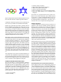
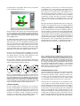
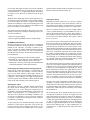
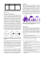
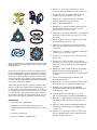
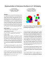
Representation of Interwoven Surfaces in 21/2D Drawing
Keith B. Wiley
University of New Mexico
Computer Science Dept.
[email protected]
Lance R. Williams
University of New Mexico
Computer Science Dept.
[email protected]
ABSTRACT
The state-of-the-art in computer drawing programs is based
on a number of concepts that are over two decades old. One
such concept is the use of layers for ordering the surfaces in a
drawing from top to bottom. Unfortunately, the use of layers
unnecessarily imposes a partial ordering on the depths of the
surfaces and prevents the user from creating a large class of
potential drawings, e.g., of Celtic knots and interwoven surfaces. In this paper we describe a novel approach which only
requires local depth ordering of segments of the boundaries
of surfaces in a drawing rather than a global depth relation between entire surfaces. Our program provides an intuitive user interface which allows a novice to create complex
drawings of interwoven surfaces that would be difficult and
time-consuming to create with standard drawing programs.
Author Keywords
A
D
A
B
B
C
C
E
D
E
F
F
Figure 1. The classic approach to representing relative surface depths is
to assign the surfaces to distinct layers. This implicitly imposes a DAG
on the surfaces such that no subset of surfaces can interweave because
this would require a cycle in the graph.
drawing programs, layers, knot diagrams, braids, surfaces,
computational topology, constraint propagation
ACM Classification Keywords
H.5.2 User Interfaces; I.3.3 Picture/Image Generation; I.3.4
Graphics Utilities; I.3.6 Methodology and Techniques
INTRODUCTION
Drawing programs originated with Sutherland’s seminal
PhD thesis in 1963, in which many recognizable components
of modern drawing programs were already present [19]. Apple’s LisaDraw 3.0, released in 1984 is a more recent example [4]. LisaDraw possessed much of the functionality
found in most modern drawing programs. In the twenty years
since LisaDraw’s release, developers of drawing programs,
e.g., [1, 3, 8, 17], have refined the basic approach, but not in
ways which deviate significantly from the established paradigm.
One function of a drawing program is to allow the creation and manipulation of drawings of overlapping surfaces,
which we call 21/2D scenes. A 21/2D scene is a representation of surfaces that is fundamentally two-dimensional, but
Permission to make digital or hard copies of all or part of this work for
personal or classroom use is granted without fee provided that copies are
not made or distributed for profit or commercial advantage and that copies
bear this notice and the full citation on the first page. To copy otherwise, or
republish, to post on servers or to redistribute to lists, requires prior specific
permission and/or a fee.
CHI 2006, April 22-27, 2006, Montréal, Québec, Canada.
Copyright 2006 ACM 1-59593-178-3/06/0004...$5.00 .
which also represents the relative depths of those surfaces
in the third dimension. Using existing programs, a drawing
can easily be created in which multiple surfaces overlap in
various subregions. When multiple surfaces overlap, the program must have a means of representing which surface is on
top for each overlapping pair of subregions. Existing drawing programs solve this problem by representing drawings
as a set of layers where each surface resides in a single layer.
For any given pair of surfaces, the one that resides in the
upper (or shallower) layer is assigned a smaller depth index and appears above wherever those two surfaces overlap. Consequently, the use of layers imposes a partial ordering, or a directed acyclic graph (DAG), on the surfaces such
that no subset of surfaces can interweave (Fig. 1). Because
such programs do not span the full space of possible 21/2D
scenes, they preclude many common drawings which a user
may wish to construct (Fig. 2).
Our research uses a more general representation as the basis for a more powerful drawing tool, called Druid. Druid
eliminates the assumption that surfaces cannot interweave.
It therefore spans a larger space of 21/2D scenes by using
a representation that makes weaker assumptions about the
drawing.
Some research has already been done on programs for constructing Celtic knotwork, e.g., Scharein’s PhD thesis [18].
Such systems, however, are limited to knot constructions,
i.e., interwoven cords. Druid, on the other hand, permits the
•
•
•
•
•
•
Figure 2. Druid permits the construction of drawings of interwoven surfaces, such as those shown here: Olympic rings and Star of David.
construction of much more general scenes in which the surfaces can be any orientable two-manifold with boundary.
Perhaps the research that most closely resembles Druid is
that by Baudelaire and Gangnet [2], which relies on planar maps as the organizing principle for a drawing tool and
map-sketching as a means to construct 21/2D scenes. Planar
maps permit the construction of overlapping curve segments,
which are subsequently pruned using map-sketching, during
which some edges are erased. Each face of the graph (an
edge-bounded region of the surface boundary graph) can be
assigned an independent color in the drawing.
With a proper erasure of edges and coloring of faces, the illusion of interwoven surfaces can be achieved. It is interesting
to note that edge erasure is not required for this method to
work and is therefore superfluous, i.e., faces can be colored
to achieve the appearance of interwoven surfaces without erasing any edges. This approach is quite similar to the best
method available in Adobe Illustrator [1] for constructing
21/2D scenes in which the user converts a series of overlapping curves into a planarized graph in which the faces can
be assigned independent colors. As such, the Baudelaire method is simply the Illustrator method with an additional (and
unnecessary) edge-erasing interaction, although their research predates the implementation of this feature in Illustrator.
These approaches do not possess the natural affordances of
21/2D scenes. The edit distances required to traverse elementally similar drawings can be quite large. In effect, these approaches aim to simplify the process of constructing spoofs,
a term we discuss at some length later in this paper.
DRAWING PROGRAM USER-INTERACTIONS
Druid uses B-splines to represent boundaries. Similar to
MacPowerUser’s iDraw [8], all shapes are splines, including shapes that may be approximated by splines, such as
rectangles and text. The assumption that all boundaries are
splines lends a uniformity to a drawing program’s interface
that makes it easier for a user to understand. There are a
number of user interactions that a spline-based drawing program should permit. These interactions include:
• Create a new boundary
• Delete a boundary
Smoothly reshape a boundary
Drag a surface (drag all of its boundaries)
Add or remove spline control points
Increase or decrease spline degree
Reverse a boundary’s sign of occlusion (discussed later)
Reverse the depth ordering of two overlapping surface
subregions.
The interface of a program should not only provide a method for each of these interactions; these methods must be
user-friendly, i.e., simple to understand and easy to use. Unfortunately, the only previous attempt to circumvent the partial ordering limitation, MediaChance’s Real-Draw Pro 3,
forces the user to use a complex and confusing interface.
Software Affordances
A software application’s interface possesses a specific set of
affordances. The term was originally coined by Gibson [5]
and later used by Norman [13, 14]. There are multiple interpretations for this term and how it should be applied to
design (see McGrenere [10]). We define the affordances of
a software user interface as the ways in which the user can
interact with the screen’s imagery. This interaction usually
involves a keyboard and a mouse. In the case of drawing
programs, use of the keyboard is generally minimized because this violates the notion of direct manipulation interfaces (discussed below). Therefore, the affordances of drawing
programs mainly consist of clicking on and dragging various
features of the visual presentation, e.g., spline control points,
with a mouse and associated cursor.
Idealized physical surfaces possess certain natural affordances. They can be stretched, translated, cut into smaller surfaces, have holes cut in them, and be lifted above or pushed
beneath one another in potentially interwoven arrangements.
They can also be colored or be made transparent. We believe that a set of affordances isomorphic to those of idealized
physical surfaces should be provided by an effective drawing
program. Unfortunately, many drawing programs do not offer such a set of isomorphic affordances. It is our belief that
while some programs, such as Real-Draw, attempt to solve
the problems posed in this research, they do so through interfaces with unnatural affordances which make the programs
complicated and non-intuitive to use. Druid’s interface possesses affordances which are isomorphic to the affordances
of the physical surfaces which are depicted. As such, it is
simpler to use, while at the same time, is more powerful than
existing drawing programs in its capability to create and edit
complex 21/2D scenes.
Direct Manipulation and Constraint-based Interfaces
In our design of Druid, we have embraced the concept of a
direct manipulation interface (see Norman and Draper [15]).
A direct manipulation interface is an interface which allows
the user to interact with the depicted object using the most
direct method possible given the I/O devices that are available. The basic premise of a drawing program as a tool which
shows the drawing as it is being constructed may seem obvious now, but it originated with the WYSIWYG concept
that came out of Xerox PARC in the 1970s (see Myers [12]),
which is a fundamental component of a direct manipulation
interface. In addition, Raisamo and Raiha applied the idea
of direct manipulation interfaces to the problem of aligning
objects in a drawing [16].
The most common application of constraints in drawing programs is gravity-snapping, where the cursor snaps to grid
points for the purpose of keeping objects aligned. A slightly
different approach snaps objects to other objects rather than
an underlying grid (see Gleicher [6]). Druid’s operation is
also based on constraints. First, Druid constrains the user
to constructing topologically valid 21/2D scenes. Second, a
user’s interaction with a drawing takes the form of a constraint, indicating the user’s intent, that guides the search process for a new legal labeling.
Stage 1 consists of programs based on representations that
can be described as layers of constant depth, and includes
virtually all existing drawing programs.
Stage 2 consists of programs based on partial orderings, but
which allow the user to define special regions of the canvas
where the partial ordering will differ from the global DAG.
To our knowledge, the only program in this category is MediaChance’s Real-Draw Pro-3 (see Voska [20]). Real-Draw
starts out with a basic layered representation, but then provides a special tool called the push-back. This tool lets the
user define a region of the canvas where the partial ordering
can be locally altered. The layer that resides at depth zero
within the selected region can be pushed down to an arbitrary depth, placing it beneath some or all of the (previously)
deeper layers (Fig. 4).
SPOOFS
With considerable effort, it is possible to create images with
existing drawing programs that depict interwoven surfaces.
However, the underlying representation in such cases is not,
and cannot be, truly interwoven. This is accomplished in existing programs by constructing one set of surfaces which has
the appearance of a completely different set. We call this sort
of illusion a spoof (Fig. 3). Spoofs represent non-generic
configurations, where various elements of a drawing are precisely aligned to create the illusion of interwoven surfaces.
Figure 4. Real-Draw provides a push-back tool, which allows the user to
define a region of the canvas and then manipulate the ordering of the
layers within that region.
(1) Start with the right ring on the
bottom. Copy just the right ring
in the selected rectangle.
(3) Place the spoof precisely
over its original position,
on top of both rings.
(2) Paste.
(4) The spoof is brittle. If either
ring is moved, the spoof breaks.
Figure 3. A spoof is a process by which the illusion of interwoven surfaces can be constructed in a layered system. The underyling representation does not match the final rendered image.
Although spoofs are a sufficient method for creating rendered images of interwoven surfaces, they are tedious to construct, requiring many steps to be performed with precision.
Furthermore, they are brittle because once a spoof has been
constructed, any alterations to the drawing will require the
spoof to be redone.
STAGES IN DRAWING PROGRAM EVOLUTION
In this section we describe a progression of drawing program functionalities leading up to Druid. This progression
classifies drawing representations in three stages of increasing generality.
Stage 3 consists of drawing programs based on representations that do not rely on any form of a partial ordering of
the surfaces. Such a representation contains only localized
information about the depths of various subregions of the
surfaces. We do not know if Druid’s representation is the
best representation of this type, but it has been proven that
Druid’s representation is sufficient to represent the full space
of 21/2D scenes (see Williams [23]).
One might ask what advantages Stage 3 drawing programs
have relative to Stage 2 drawing programs. One problem is
that Real-Draw’s interface for manipulating surfaces is somewhat awkward. Because the push-back object does not
reflect the way humans perceive and reason about surfaces,
it is not a natural tool for editing drawings of overlapping
surfaces, i.e., it does not possess natural affordances (affordances that are isomorphic between the drawing being edited
and the surfaces which are depicted).
More significantly, Real-Draw does not span the space of
21/2D scenes. There are two situations where this can arise.
The first occurs when the user attempts to create a surface
that overlaps itself. Each surface in Real-Draw is represented
by a single label in the global surface DAG. A push-back
only allows the reordering of layers based on labels in the
DAG. Two overlapping subregions of the same surface will
have the same global label, and that label will only occur
once in the DAG. Consequently, there is no way to represent
a self-overlapping surface (Fig. 5).
Figure 5. Real-Draw cannot properly represent self-overlapping surfaces. Since a surface has only one label in the surface layer list, there is
no way to manipulate the depth ordering of multiple subregions belonging to a single surface. For this reason, Real-Draw cannot represent
self-overlapping surfaces.
An additional problem with Real-Draw is that the push-back
object only allows the depth zero object to be pushed down.
Therefore, there is no way to manipulate the ordering of deeper layers. If surfaces are opaque this does not matter since
only the depth zero surface will be visible. However, if surfaces are transparent, then the ordering of deeper layers might
affect (depending on the exact transparency model used) the
appearance of a region where multiple surfaces overlap.
In theory, the push-back could be expanded in its power
to allow a more comprehensive manipulation of the surface depths. However, the more serious problem of selfoverlapping surfaces would remain unaddressed.
Druid’s Stage 3 approach is more powerful in both of these regards since it naturally represents both self-overlapping
surfaces and transparent surfaces with ease.
0
0
1
0
1
0
0
0
1
1
0
This paper describes the algorithm Druid uses to assign a labeling to a knot-diagram. The process of assigning a labeling
is similar to Huffman’s scene-labeling (see Huffman [7]),
in which he developed a system for labeling the edges of a
scene of stacked blocks. In Druid. the labeling consists of
signs-of-occlusion, crossing-states, and segment depth indices. The labeling scheme is a set of local constraints on the
relative depths of the four boundary segments that meet at a
crossing (Fig. 7). If every crossing in a labeled knot-diagram
satisfies the labeling scheme, the labeling is a legal labeling
and represents a scene of topologically valid surfaces. Legal labelings can be rendered, i.e., translated into images in
which the interiors of surfaces are filled with solid color.
x
y ≥x
y+1
x
Figure 7. The labeling scheme (see Williams [23]) is a simple set of constraints on the depths of the four boundary segments that meet at a crossing. If every crossing in a labeling honors the labeling scheme then the
labeling is legal and can be rendered. x is the depth of the upper boundary. The upper boundary must have the same depth on both sides of
the crossing. y is the depth of the unoccluded half of the lower boundary. The lower boundary must have a depth of y + 1 in the occluded
region (shaded), as defined by the upper boundary’s sign of occlusion.
Finally, the lower boundary must reside beneath the upper boundary,
thus, y must be greater than or equal to x.
0
0
1
0
Druid represents a 21/2D scene as a labeled knot-diagram
(see Williams [23]). A knot-diagram is a projection of a set
of closed curves onto a plane and indicates which curve is
above wherever two intersect (Fig. 6, left). Williams extended ordinary knot-diagrams to include a sign of occlusion
for every boundary and a depth index for every boundary
segment (Fig. 6, right). The sign of occlusion is illustrated
with an arrow and denotes a bounded surface to the right
with respect to a traversal of the boundary in the arrow’s direction.
1 0
1
0
0 0
1
0
Figure 6. A knot-diagram (left) is a projection of a set of closed curves
onto a plane together with indications of which is on top at every crossing. A labeled knot-diagram (right, see Williams [23]) is a knot-diagram
with a sign of occlusion for every boundary and a depth index for every
boundary segment. Arrows show the signs of occlusion for the boundaries, always denoting a surface bounded to the right of a boundary with
respect to travel of the boundary in the direction of the arrow.
LABELING SCHEME
In order to build a Stage 3 drawing tool, it is necessary to
develop a fundamentally new approach for the representation of drawings. Existing drawing programs represent a drawing as a set of regions which comprise the interiors of a set
of surfaces. In constrast, a Stage 3 program represents the
boundaries of surfaces and is not concerned with the regions interior to a surface until the final rendering step.
DEMONSTRATION OF DRUID
Fig. 8 demonstrates how Druid is used. Druid uses closed Bsplines to represent the boundaries of surfaces. Spline control points are defined in either a clockwise order to create solids (A) or in a counter-clockwise order to create holes
(C). Crossings can be clicked to reverse the relative depths
of overlapping subregions (B and D). This is called a flip.
Note that there is a natural logic to the operations in Fig.
8. For example, to alter the depth ordering of various overlapping subregions, the user merely clicks on a crossing to
invert its crossing-state. Druid then does all of the computation necessary to keep the labeling legal. This computation
consists of searching the space of legal labelings for a labeling which satisfies the constraint represented by the new
crossing state. Compare this mode of interaction with either the spoof approach associated with Stage 1 drawing programs or with the push-back approach associated with Sta-
ge 2 drawing programs, i.e., Real-Draw. Construction of a
spoof that appears like D would be quite tedious. Worse yet,
to invert the relative depth ordering within a subregion, the
spoof would have to be completely rebuilt. In Real-Draw,
push-back objects would have to be explicitly created for
each desired subregion and would have to be maintained if
the user were to move the surfaces around.
a barrier between themselves and the drawing. In our case,
this contributes to the user’s perception that he is interacting
with real surfaces (see Norman and Draper [15]).
0
[0-1]
[0-1]
0
[0-2]
[0-1]
[0-1]
[0-1]
0
0
0
[0-2] [0-1]
[0-2]
[0-1]
[0-1]
0
Figure 9. For a particular labeled knot-diagram, each boundary segment has a range of possible depths that it can assume, depending on
how many surface subregions it overlaps. The size of L for each of the
three drawings shown from left to right is 1, 16, and 110592 respectively. This figure illustrates the fact that the size of L scales explosively
relative to the complexity of the drawing.
Calculating the Depth Ranges for a Labeled Knot-Diagram
Figure 8. Demonstration of Druid. Spline control points are defined in
either a clockwise order to create solids (A) or in a counter-clockwise
order to create holes (C). Crossings are clicked to flip overlapping surface subregions (B and D).
The depth range that each boundary segment can assume
must be calculated before the figure can be labeled. To solve
this problem we have framed the task of finding the depth
ranges for all segments for a particular topology as a new
kind of labeling problem, similar to the labeling problem discussed earlier. The challenge is to label a knot-diagram in the
fashion shown in Fig. 9, where crossing-states remain unspecified but all segments have a range of possible depths associated with them. This relaxed labeling problem (Fig. 10) is
similar to the original labeling problem where the goal is to
assign a single index to each segment. However, in a relaxed labeling the index is the depth range for a segment, i.e.,
the maximum depth that a segment can assume among all
topologically valid labelings. We have devised an iterative
algorithm that determines the depth ranges by acting directly on the knot-diagram in a series of iterative passes, starting
from depth zero and accumulating maximum depths for the
segments incrementally.
LABELED KNOT-DIAGRAM SPACES
Given an unlabeled drawing t ∈ T in the space of all possible
drawings T, there exists a set of possible labelings that can be
assigned to that drawing, L(t ∈ T). C(t) ⊆ L(t) is the subset
of L consisting of consistent (or legal) labelings. When the
user causes a change to the drawing, Druid must search L(t)
for a new legal labeling, i.e., an instance of C(t).
The organization of the search process is motivated by the
primary goal of finding the minimum-difference labeling
with respect to the labeling prior to the interaction. The
user communicates his intent by specifying a single constraint on the new labeling. Druid then deduces the remaining constraints by searching for a legal labeling that satisfies the user’s explicit constraint. In this way, Druid deduces
the user’s intentions automatically, thereby minimizing the
user’s effort.
Graph Distance Between Labelings
For drawings of a moderate size L can be extremely large
given that we want Druid to perform fast enough to not annoy the user. Fast feedback is an important aspect of direct
manipulation interfaces. Norman and Draper argue that fast
feedback reduces the user’s awareness of the computer as
D
x
x+1 B
A x
x+1
C
Figure 10. The relaxed labeling scheme is a set of constraints on the
depth ranges of the four boundary segments that meet at a crossing.
Each boundary occludes the half-plane on its right. Thus, for the two
boundaries meeting at a crossing, one half of each boundary will lie in
the unoccluded half-plane of the opposing boundary, and the other half
will lie in the potentially occluded half-plane of the opposing boundary.
The shaded regions in the figure show the potentially occluded halfplanes of each boundary. Segments B and C are potentially occluded.
The labeling scheme requires that the potentially occluded segments of
a crossing have a depth range that is one greater than the depth range
of the unoccluded segments and that the two boundaries have the same
depth ranges as each other.
EDITING 21/2D SCENES
Note that Druid is much more than just an editor for labeled
knot-diagrams. In a simpler program, a user might manually
edit crossing-states and segment depths without constraint.
There are two major problems with this approach. The first
is that many of the knot-diagrams a user might create would
be illegal and could not be rendered. Thus, the burden would
fall upon the user to carefully manage the knot-diagram at
all times. The second problem is that the interface for such
a program would provide affordances that are not isomorphic with those of 21/2D scenes. The user would not have
the experience that he is editing a 21/2D scene, but rather the
experience that he is managing the details of a labeled knotdiagram. To summarize, by virtue of its use of constraint
propagation, Druid is actually an editor for 21/2D scenes,
not for labeled knot-diagrams.
Unlike Druid, Real-Draw basically is an editor for its internal representation, a global DAG with localized regions
specifying local DAG changes. The manipulations the user
performs in Real-Draw equate edit distances of one with
representation distances of one. Therefore, the user is directly manipulating Real-Draw’s representation. This design
is awkward, since there are situations where realizing the
user’s intentions may require navigating a large representation distance to travel a small 21/2D scene transformation
distance.
Druid’s power derives from its ability to quickly search
through the space of labeled knot-diagrams for legal labelings. The reason the user has such a qualitatively different
experience when using Druid is that elemental scene transformations can be accomplished with single mouse clicks.
It is this isomorphism between editing operations and 21/2D
scene transformations that makes Druid so novel.
USER INTERACTIONS
Several possible user interactions were listed at the beginning of this paper. The effects of these interactions on the
labeled knot-diagram can be grouped into two major categories:
• Labeling-preserving interactions
• Interactions requiring relabeling.
Labeling-preserving interactions are interactions in which
the topology of the labeled knot-diagram does not change.
In constrast, interactions requiring relabeling are of the following types:
• Drags or reshapes that create new crossings
• Drags or reshapes that delete existing crossings
• Drags or reshapes that change the order of existing crossings along the boundaries
• Change of the crossing-state of a crossing (“flipping” a
crossing)
• Change of the sign occlusion of a boundary (flipping a
sign of occlusion).
In the following sections we describe how these two kinds
of interactions are handled by Druid.
Labeling-Preserving Interactions
Ideally, Druid should preserve the labeling during user interactions whenever possible because we assume that the
user does not want the labeling to change arbitrarily while he is editing a drawing. When one boundary is dragged
over another, the crossings involved in both will move. The
goal of preserving the crossings’ states during such interactions precludes the naive method of deletion and rediscovery of crossings since such an approach would destroy the
crossing-states, and the knot-diagram would have to be relabeled. While relabeling can generally be performed fairly
quickly, it is also crucial that the labeling following a nontopology-altering interaction match the labeling prior to the
interaction. Because there is no way of guaranteeing that the
crossing-states discovered after relabeling will match the old
crossing-states, the naive method is infeasible. The only alternative is to avoid the relabeling whenever possible.
original
intersection
location
moving
boundary
before
jump
moving
boundary
after
jump
a
b
A
Iteration 0
stationary
boundary
Iteration 1
c
B
Iteration 2
d
D
C
Iteration 3
Iteration 4
Iteration 5
Figure 11. The sequence of drawings shown here illustrate successive iterations of the crossing projection algorithm. Thick line segments
show the segment pair associated with the crossing at the beginning of
each iteration. Circles show the intersections of the lines containing the
segments. Lowercase labeled segments (a-d) show the segment that will
be switched out of the pair assignment at the end of that iteration. Uppercase labeled segments (A-D) show the segment that will be switched
into the pair assignment at the end of an iteration. After a timestep, the
algorithm tests the original segments assigned to the crossing (shown
in Iteration 1). In the example illustrated, the segments no longer intersect. Since the error (the distance past the end of each segment to the
point of intersection of the lines containing the segment pair) is greater
for the moving boundary at the beginning of Iteration 1, the moving
boundary segment assigned to the crossing’s segment-pair assignment
will be switched from a to A. The process continues until a pair of segments is found that actually intersect, as shown at the beginning of Iteration 5.
For some interactions, e.g., drags and reshapes which do not
alter the topology, the labeling can be preserved by projecting crossings along the paths they follow on the boundaries
(Fig. 11). The process of projecting crossings to their new
locations during a move or reshape of a boundary is called
crossing projection. The goal is to analyze and follow the
path that a crossing follows around a boundary. This algorithm is relatively complex because there are a number of
special cases that must be properly detected and handled,
e.g., the appearance of new crossings or the disappearance
of existing crossings. It is also possible for crossings to pass
one another on a boundary as a result of a user interaction.
Projection is accomplished primarily by following a crossing from one segment to the next around a boundary until
the crossing’s new location is determined, (Fig. 11).
User Interactions Requiring Relabeling
While some user interactions do not require relabeling, other
interactions cause changes to the knot-diagram’s topology,
and therefore, require a search for a new legal labeling. Devising an algorithm that can find the minimum difference
labeling quickly is difficult because the search space may be
extremely large relative to the complexity of the drawing.
The process for relabeling a labeled knot-diagram is described in the next section.
FINDING A LEGAL LABELING
When the user causes a change that invalidates the current
labeling, Druid must find a minimum difference legal labeling as quickly as possible. We will describe how this is accomplished in the case of a crossing flip user-interaction, i.e.,
the user clicks on a crossing to flip its crossing-state, and in
doing so, inverts the depth order of the two subregions associated with that crossing.
When the user clicks on a crossing to flip its crossing-state,
he imposes a constraint that is inconsistent with the present
labeling. Druid then searches for a legal labeling that satisfies the user’s constraint. This will often require changes on
the labeling, such as the crossing-states of other crossings or
the depths assigned to various boundary segments. Thus, the
search solves a constrant-satisfaction problem were the user
specifies the initial constraint.
Constraint-Propagation
The search takes the form of a constraint-propagation process similar to Waltz filtering (see Waltz [21]). Waltz’s
research illustrated how certain combinatorially complex
graph-labeling problems can be reduced to unique solutions
through a process called constraint-propagation. In a graphlabeling problem, when one vertex of a graph is labeled, this
constrains adjacent vertices, which in turn propagate their
own constraints deeper into the graph. By means of this process, it is often the case that an apparently ambiguous labeling problem can be reduced to a single consistent labeling.
Boundary Traversal During the Search
In Druid, constraints are applied as the search process explores the labeling space through a set of boundary traversals. A boundary traversal begins at an arbitrary location on
a boundary with a specified depth and visits each segment on
the boundary, until it returns to the starting location. The purpose of performing a boundary traversal is to test the traversal’s legality using the zero integration rule. This rule guarantees that a traversal ends at the same depth that it started
at, which is a requirement of a legal labeling.
Note that once a boundary traversal has begun, the depth
changes that occur during the traversal are uniquely determined. There are only three situations which can occur when a
traversal reaches a crossing:
• If the boundary being traversed is on top at the crossing,
the depth does not change.
• If the boundary being traversed goes under at the crossing,
the depth increases by one.
• If the boundary being traversed comes up at the crossing,
the depth decreases by one.
While the differences in depth around a boundary are uniquely determined, the depth of the initial segment of the
traversal is constrained, but not uniquely. The depth of the
initial segment must be within its depth range, as shown in
Fig. 9, but since any depth in this range might be the depth
of the optimum solution, all depths in the range must be tested. This is accomplished by calling the boundary traversal
process within a loop that enumerates the possible depths for
the initial segment.
At this point, we have described how a single boundary traversal is effected, and we have specified that the goal of a
boundary traversal is to test the boundary with the zero integration rule. Next we will describe how the boundary traversal process is invoked with the context of a larger treesearch which performs multiple boundary traversals during
the course of the search for a minimum difference labeling.
Structuring the Search
The search for a minimum difference labeling is a depth first
search. Each of the possible depths for the initial segment
of a traversal is the root of a distinct search tree. The search
trees branch when a boundary reaches a crossing; each of the
two crossing states is the root of a distinct subtree.
The decision about which boundaries are traversed during
the search is managed using the touched boundary list, a
list of boundaries that have been crossed during the traversal
of other boundaries. As boundaries are crossed, or touched,
they are appended to the end of the touched boundary list.
The touched boundary list is initially seeded with all boundaries that are illegal, i.e., all boundaries that have at least
one illegal crossing. In the case of a crossing flip, the flipped
crossing will initially always be illegal.
The following is a description of the entire backtracking
search process. An empty touched boundary list is seeded
with all illegal boundaries. The next boundary to be traversed is then chosen from the front of the touched boundary
list. This boundary is then traversed repeatedly within a loop
which enumerates each of the possible depths for the initial
segment of that boundary.
As the traversal visits each crossing of a boundary, the crossed boundaries are appended to the touched boundary list.
When all combinations of crossing-states for all crossings
on the traversal boundary have been enumerated, a traversal
is completed. If the traversal satisfies the zero integration rule, the traversal process restarts with the next boundary on
the touched boundary list. If the traversal ends illegally the
process backtracks to the last unflipped crossing, flips that
crossing’s state, and continues.
If a traversal ends legally and there are no more boundaries
on the touched boundary list, the search has reached a leaf, or
a potential solution, i.e., a legally labeled figure. The solution
is assigned a score based on its difference from the prior
labeling.
When the entire depth range for the initial segment has been enumerated, the next boundary on the touched boundary
list is selected. When the search is completed, the solution
with the lowest difference relative to the labeling prior to the
search is accepted. The new labeling is then displayed and
the user can initiate a new interaction.
The difference between labelings discovered by the backtracking search process and the prior labeling increases under two circumstances:
• When a crossing is flipped
• When a segment depth differs from its original depth.
OPTIMIZING THE SEARCH
Because of the large size of the search space, searching for
the minimum-difference labeling might take a considerable
amount of time. Therefore, we employ a number of strategies in an effort to find the minimum-difference labeling
quickly enough to provide the user with a reasonable turnaround time. The strategies are broken down into three major classifications:
• Choosing good boundary traversal starting segments
• Bounding the search using the current minimum difference to avoid a full enumeration of the search space
• Ordering the search to produce tight search bounds based
on minimum difference earlier rather than later.
Choosing good boundary traversal starting segments
Each time an untraversed boundary is selected from the
touched-boundary list, that boundary is traversed within a
loop over the initial segment’s depth range. Naively, we
might choose the starting segment arbitrarily. However, Fig.
9 suggests a better strategy. It is highly advantageous to
choose a segment on the boundary with the minimum depth
range for the entire boundary as the starting segment.
Bounding the search
The difference between a candidate labeling found during
the search and the labeling prior to the search is accumulated, one δ at a time, during the search process as
the boundary-traversal algorithm branches–either preserving
features of the labeling (δ = 0) or altering them (δ = 1).
The sum of all δ ’s between two labelings is termed L∆ . Notice that the accumulated δ can never decrease and that it
is possible to exploit this fact during the search to improve
performance by bounding.
As the search proceeds, candidate labelings will be found,
and their L∆ will be known. This value can be used to improve the efficiency of the remaining search. Since L∆ ’s cannot decrease as subtrees are expanded, there is no reason to
expand a subtree that has already accumulated an L∆ greater
than that of the best solution found so far.
Ordering the Search
Bounding the search works best if we can find a solution
with a tight bound early in the search. Because certain labelings have a better chance of being optimal, we order the
search so that those labelings are likely to be explored first.
There are a number of criteria we can use to judge whether
or not a potential labeling is a good candidate for early expansion. We assume that the user expects most changes to
occur within a relatively small region surrounding the location of the user specified constraint. This region is termed
the area of interest.
If we order the search so that regions of the search space within the area of interest are explored first, then we can effectively enumerate all possible labelings which differ from the
prior labeling only within the area of interest before considering labelings which differ from the prior labeling outside
of this area. Ordering the search in this manner has two benefits. First, it most likely reflects the user’s intent. Second,
the number of potential changes in a compact area is significantly smaller than the number of potential changes in the
entire drawing, so we will find any solutions where changes
are restricted to that area much more rapidly than we would
find solutions where changes are unrestricted.
We search regions near the area of interest early in the search
process by executing the depth first search described above
within an iterative deepening loop, which is commonly used
in game tree search algorithms (see Marsland [9]). We do
this by calculating, in advance, the graph distance between
each crossing and the crossing in the center of the user’s area
of interest. We then perform the depth first search in a loop
where the search horizon increases by one after every iteration. As a boundary is traversed to test the zero integration
rule, no crossings beyond the current horizon are expanded.
Not only does iterative deepening expand subtrees corresponding to crossings within the area of interest first and
which are therefore more likely related to the user’s goal, but
it also finds labelings with small L∆ ’s which provide stronger
bounds early, which increases the efficiency of the branch
and bound search.
The following table shows sample running times for some
crossing-flips. Interactions A and B are toggles back and
forth of the bridge between the two halves of the anthropomorphic figure in the top left drawing of Fig. 14. Interactions
C and D are toggles back and forth of the overlapping letters
’U’ and ’I’ in the top right drawing of Fig. 14. Interactions
E and F are toggles back and forth of one of the overlapping
regions for the drawing in Fig. 13. These running times were collected on a 1.6 GHz G5 Powermac and represent nine
trials each.
Interaction
A
B
C
D
E
F
Edges Traversed
8734
6707
575
1435
1463
1463
Median seconds
.62
.68
.04
.09
.19
.19
RENDERING
In summary, we observe that Druid’s response time to a crossing flip interaction for typical drawings is consistently less
than one second.
BOUNDARY GROUPING WITH CUTS
One feature that is common to almost all drawing programs
is the ability to group objects together. Groups are usually provided so that transformations like translation, scaling,
and rotation can be applied to all of the members of a group.
Boundary groups are not required for Druid to legally label
a drawing. However, boundary groups provide a basis for
translation of a surface with multiple boundaries, and more importantly, can be used to eliminate ambiguities about
which surfaces boundaries belong to. For example, in Fig.
12 (left), there exists an ambiguity as to whether boundary
B bounds a surface below boundary A, above boundary A,
or is part of the same surface as boundary A. If a the user
were to attempt to place a third boundary that overlaps the
ambiguous surface of A and B, there is the possibility that
the third surface might be placed between boundaries A and
B. Clearly, if the user’s intent is for boundaries A and B to
be part of the same surface, then such a placement violates
the user’s expectations about the effects of his interactions.
Grouping boundaries can minimize this kind of problem.
A
Cut
Gap
B
Figure 12. A cut can be thought of as a scissor cut through a surface connecting two boundaries of that surface. Cuts are used to group
boundaries together for group transformations like translation, scaling,
and rotation.
There are parallels between the approach used in Druid to
render labeled knot-diagrams and algorithms used for hidden surface removal in computer graphics, e.g., the WeilerAtherton algorithm [22]. Rendering consists of converting
the labeled knot-diagram (Fig. 13, left) to an image with solid fills for contiguous bounded regions of the canvas. To
render opaque surfaces, we only need to find the depth zero
surface for each region (Fig. 13, center). However, to render
transparent surfaces we must find the full depth ordering of
all surfaces for each region so that a transparent coloring model, such as Metelli’s episcotister model (see Metelli [11]),
can be applied (Fig. 13, right).
Figure 13. A labeled knot-diagram (left) can be rendered into a surface
rendering such as those shown above (center, right). The surfaces associated with each region must be determined so that a proper coloring
for that region can be assigned to the final image.
CONCLUSIONS
All drawing programs must have a way to distinguish which
surface is on top for any overlapping pair of subregions. Existing drawing programs solve this problem by assigning surfaces to distinct layers in depth. Consequently, interwoven
sets of surfaces cannot be represented, thus precluding drawings of a large class of 21/2D scenes. We have developed
an innovative new drawing program with the following major capabilities:
• Naturally representing a more general class of drawings,
i.e., drawings in which surfaces interweave
• Providing user-interactions in the form of user specified
constraints which are automatically propagated to maintain topological validity of the representation.
Specific contributions of this work are as follows:
Druid automatically finds and maintains boundary groups
without requiring any input from the user. It does this by
finding and maintaining cuts. A cut can be thought of as a
scissor cut through a surface connecting two boundaries that
belong to a single surface. A cut converts two boundaries of
a surface into a single boundary. See Fig. 12 (center, right).
If a cut can be found between the two boundaries, as shown
in Fig. 12, then the two boundaries are demonstrably part of
the same surface and can be grouped.
Observe that the discovery of a cut between two boundaries
effectively connects the two boundaries into a single closed
boundary. Cuts effectively reduce the number of boundaries
in a drawing, by one per cut. Consequently, they reduce the
overall complexity of a drawing, thereby reducing the size of
the search space and making the search significantly faster.
• Use of labeled knot-diagrams as the basis for a more general drawing tool capable of representing drawings of interwoven surfaces
• Development of a method for projection of the locations
of crossings of surface boundary components after move
and reshape interactions
• Development of a relaxation method for determining
depth ranges for boundary segments in a labeled knotdiagram based representation
• Development of a branch and bound search method for
efficiently finding minimum difference labelings with respect to the labeling preceding a user action
• Introduction of the notion of cuts for representing surfaces
with multiple boundary components and for reduction of
the search space.
5. Gibson, J. J., The Ecological Approach to Visual
Perception, Houghton Mifflin Co., Boston, MA, 1979.
6. Gleicher, M., Briar: A Constraint-Based Drawing
Program, Proc. of CHI, Monterey, CA, 1992.
7. Huffman, D. A., Impossible Objects as Nonsense
Sentences, Machine Intelligence, 6, 1971.
c
8. iDraw, 2005
MacPowerUser.
9. Marsland, T. A., and M. Campbell, Parallel Search of
Strongly Ordered Game Trees, ACM Computing
Surveys, 14 (4), pp. 533-551, 1982.
10. McGrenere, J., and W. Ho, Affordances: Clarifying and
Evolving a Concept, Graphics Interface, pp. 179-186,
May 2000.
11. Metelli, F., The Perception of Transparency, Scientific
American, 230 (4), pp. 90-98, 1974.
12. Myers, B. A., A Brief History of Human Computer
Interaction Technology, ACM Interactions, 5 (2), pp.
44-54, 1998.
13. Norman, D. A., Affordance, Conventions, and Design,
ACM Interactions, pp. 38-43, 1999.
14. Norman, D. A., The Design of Everyday Things, Basic
Books, 2002.
Figure 14. Shown above are several examples of artwork created with
Druid. The construction and maintenance of these drawings is simple
and straightforward.
Druid uses a more general surface representation than is
used by existing drawing programs. It represents surfaces by
their closed boundaries and only maintains local constraints
on the ways in which boundaries can cross one another. These local constraints do not impose a global layering on the
elements of the drawing and therefore permit the construction of scenes of interwoven surfaces.
Additionally, Druid’s interface provides the natural affordances of 21/2D scenes in that actions performed by the user
are isomorphic to elemental transformations of 21/2D scenes. Using Druid is easy because it operates in a way which
is consistent with a user’s intuition about physical surfaces.
its affordances minimize the effort required of the user and
decrease the time required to construct complex drawings.
REFERENCES
c
1. Adobe Illustrator, 2005
Adobe.
2. Baudelaire, P., and M. Gangnet, Planar Maps: An
Interaction Paradigm for Graphic Design, Proc. of CHI,
1989.
c
3. Coreldraw, 2005
Corel.
4. Craig, D., LisaDraw 3.0 manual, 1984.
15. Norman, D. A., and S. W. Draper, User Centered
System Design: New Perspectives on Human-Computer
Interaction, Lawrence Erlbaum Associates, Hillsdale,
NJ, 1986.
16. Raisamo, R., and K-J Räihä, Techniques for Aligning
Objects in Drawing Programs, Department of
Computer Science, Univ. of Tampere, Technical Report
A-1996-5.
17. Sato, T., and B. Smith, Xfig User Manual, 2002.
http://xfig.org/userman/
18. Scharein, R. G. Interactive Topological Drawing. PhD
dissertation, University of British Columbia, 1998.
19. Sutherland, I. E., Sketchpad: A Man-Machine
Graphical Communication System, PhD dissertation,
Cambridge Univ., 1963.
20. Voska, R., Real-Draw manual, pp. 67-72, 2003.
http://www.mediachance.com/files/RealDrawPDF.zip
21. Waltz, D. L., Understanding Line Drawings of Scenes
with Shadows, McGraw-Hill, New York, pp. 19-92,
1975.
22. Weiler, K., and P. Atherton, Hidden Surface Removal
Using Polygon Area Sorting, ACM SIGGRAPH, pp.
214-222, 1977.
23. Williams, L. R., Perceptual Completion of Occluded
Surfaces, PhD dissertation, Univ. of Massachusetts at
Amherst, Amherst, MA, 1994.