Download MECHANICAL LAB Text - Physics and Astronomy

PHYS 493L
Call #28340
Monday and Wednesday 1400-1650 hr
Room P&A 116
Instructor: Paul R. Schwoebel
Physics and Astronomy Building Room 122
Phone: 277-2616
E-mail: kas.unm.edu
Office hours: By appointment
Text (optional): Building Scientific Apparatus, 3rd edition, by John Moore et al, (Cambridge
University Press, 4th ed. 2009) Some reading in this book will be required. Other reading
material will be recommended as it pertains to a particular lab element.
Purpose: Senior Lab will expose students to the diverse experimental techniques required of
a graduate student or professional scientist. These techniques will be developed with the
hands-on experience gained through a series of experiments that each require multiple class
sessions. These experiments will involve holography, elementary particle decay, Doppler
shifts, interference phenomena, and gas discharges. The student will be exposed to a variety
of important techniques including interferometry, precision timing and coincidence
techniques, particle detection, and sensitive velocity measurements. The laboratory will also
include an element devoted to elementary aspects of machine shop practice and an element
in which the student participates in the development of a new experiment that will be come a
permanent addition to the Senior Lab.
Grading: Grades will be based on your performance in the laboratory, such as thorough,
complete laboratory notebooks, experimental analysis, and laboratory reports. In addition,
each student will be given a one-half hour oral final exam. Laboratory performance and the
oral exam will be, respectively, 85% and 15% of your final grade. Attendance is required.
You will need to complete four laboratory elements that must include laboratories 1 and 2.
Laboratory 3 is strongly recommended and can only be taken following completion of
Laboratory 1. The time required to complete a lab element will vary depending on the
particular lab; however, plan to spend roughly four weeks of class sessions on each. Lab
reports will be turned in for grading within 2 weeks of their completion. If experiments are
performed with a partner, each student should keep their own laboratory note book and write
their own laboratory reports.
Laboratory Reports: Use the standard format for laboratory reports.*
1. Abstract
2. Introduction
3. Theory
4. Experimental Apparatus
5. Results
6. Discussion & Conclusions
7. References (References are to be to peer reviewed journal articles or books)
Reports should appear as they would in a scientific journal, with graphics embedded in
the text.
*The write-up for Laboratory 3 has some unique requirements as specified in the manual
for Laboratory 3.
1
493L: LABORATORY SAFETY
Department of Physics and Astronomy University of New Mexico
Elements of this laboratory class pose certain hazards. No instructions can substitute for
common sense. If you are unclear about something ask the instructor or TA. Safety
topics include: Machine Shop Safety, Laser Safety, High Voltage Safety, and Radiation
Safety. Safety rules and guidelines are designed to reduce the possibility of accidents in
routine situations. In a research laboratory where much equipment is custom made there
is no routine, and there is no safety rule or policy that can substitute for an intelligent and
careful handling of the equipment. The following notes are intended to make you aware
of the risks of working in the Senior and Optics Laboratories.
Machine Shop Safety
Some basic directions are given in the lab write up. Duplicate and additional items are
listed below:
• Never work alone in the shop.
• Safety glasses must be worn in the shop at all times.
• Do not enter the shop with bare feet, sandals, slippers, or open toed shoes.
• Tie back long hair.
• Do not wear loose clothing or jewelry.
• Maintain a clean work area.
• Do not touch chips while the machine is operating.
• Do not leave chuck keys in chucks.
• Secure all work (clamp in vice, chuck, etc.).
Laser Safety
For a complete introduction to laser safety see:
https://www.osha.gov/SLTC/laserhazards/
The American National Standard Institute (ANSI) has classified lasers according to what
they perceive as hazard level. Class IIIb and class IV lasers are considered as
hazardous. The HeNe lasers used in the experiments you will be doing typically will not
cause permanent eye damage, however, it is good practice to:
• Never look directly at the beam of the laser.
• Keep the laser beam in one horizontal plane close to the table.
• Never bend down to the table level.
We have purposely chosen to have the optical table surfaces as low as possible which
reduces the chances of having your eyes at the beam height. Low chairs are not allowed
in the lab. Sitting accommodations are limited to high stools.
High Voltage (& Line Voltage) Safety
You should supplement the following general electrical safety description with reading at:
http://www.osha.gov/SLTC/electrical/index.html
The following guidelines are to protect you from potentially deadly electrical shock
hazards as well as the equipment from accidental damage. Note that the danger to you
is not only in your body providing a conducting path, particularly through your heart. Any
involuntary muscle contractions caused by a shock, while perhaps harmless in
themselves, may cause collateral damage due to contact with sharp edges and points
2
inside various things like stamped sheet metal shields and the cut ends of component
leads. In addition, the reflex may result in contact with other electrically live parts.
• Don't work alone because in the event of an emergency another person's presence
may be essential.
• Always keep one hand in your pocket when near a line-powered or high voltage
system.
Radiation Safety
For a complete introduction to radiation safety see: http://www.osha.gov/SLTC/radiation/
Several types of radioactive sources will be encountered in the laboratory. Sources you
will use in this laboratory are sealed, low activity sources and therefore present no health
issues. NEVER eat, drink, or smoke in the laboratory. Wash your hands at the
conclusion of each laboratory session. Sealed gamma ray sources having activities of ~
1 µCi can be handled with your fingers. For sealed and unsealed source of roughly 10
µCi or greater use tongs or other devices - Do not handle directly.
3
4
Certification: Return this signed statement to the instructor: I have read and understood
the document on laboratory safety for Physics 493L and agree to follow these rules
when in the laboratory.
Your Name Printed: _______________________________
Signature: ________________________________
Date: __________________
5
LAB 1: Mechanical Practices in Experimental Science
Paul R. Schwoebel and Anthony Gravagne
Purpose
Introduce the student to mechanical practices used in the design and construction of
scientific apparatus through exposure to mechanical drafting and the fundamental
operations performed in a machine shop
Reading Assignment
Chapter 1: Building Scientific Apparatus, 3rd edition, by John Moore, Christopher Davis
and Michael Coplan (Perseus Books, Cambridge MA, 2003) on reserve in the Centennial
Livrary. Familiarity with the material in Chapter 2 is useful for future reference.
Background
The experimental scientist must routinely design and construct scientific apparatus in
order to conduct research. Advanced undergraduate and graduate students in the sciences
typically have an introductory electronics class/lab. Often, however, students are not
introduced to the mechanical aspects of designing and constructing scientific apparatus
until after they begin their graduate research. The student’s research career is greatly
facilitated if they acquire the proper foundations in these mechanical practices as an
undergraduate.
The mechanical aspects of building scientific apparatus involve conceptualizing the
requirement, producing a mechanical drawing that defines the apparatus to fulfill that
requirement, and fabricating the apparatus to the necessary specifications. As an
advanced undergraduate or graduate student you will often be required to accomplish all
of these tasks. As a practicing scientist, most often you will perform tasks one and two
and submit task three to a professional machine shop. In either case, understanding the
basic principles of metal working, glass blowing, and materials joining will aid you in
making mechanical drawings to communicate your needs and designing apparatus to
fulfill these needs.
Mechanical Drawing
The book, Building Scientific Apparatus, describes the basics of mechanical drawing.
More complete treatments1 can be consulted as your skill levels and needs grow. Modern
mechanical drawing is done with the aid of computer programs, referred to a ComputerAided Drafting (CAD) programs, developed specifically for this task. The limited
drawing required for this module will only require pencil, graph paper, a scale, a right
triangle, and a compass. Feel free to use computer software to make the drawing if you
have some available.
1-1
Shop Safety
The first class session on will be spent will be spent in the shop actually applying some of
the fabrication techniques about which you have been reading. Of utmost importance is
your safety in the shop. While you are working in the shop it is REQUIRED that you:
1. Wear safety glasses at all times
2. Do not wear open-toe shoes such as sandals or flip flops
3. Secure or tie back loose clothing and long hair
4. Remove all jewelry, especially includes rings, watches, and necklaces
5. Only use brushes to remove metal chips from machines
6. Do not use compressed air to clean yourself or the machines
7. Do not use earbuds, iPods, cell phone or other portable devices
8. Do not use machine tool practices that are not approved by the instructor
9. Focus on the work you are doing
10. Do not work in the shop while under the influence of drugs or alcohol. This includes
any prescription drugs which could cause drowsiness, lightheadedness, or
disorientation. If you have a question it is much better to ask the shop personnel for help than to proceed
with an operation with which you are unfamiliar.
Appended is a form to read and sign acknowledging you have read and understood the
aforementioned safety rules. Give the signed form to the shop foreman on your first day
of the Mechanical Practices Lab.
Machine Shop Practices
During the first class period you will go to the machine shop and be introduced to the
basic equipment by one of the machinists. Over the course of the remaining 4 weeks
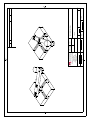
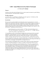
under the machinist’s supervision you will then each fabricate a fun two-slider handcrank device, of which a 3D CAD drawing is shown below. A mechanical drawing of the
hand-crank device assembly and the parts you will fabricate is also appended to this
write-up. Print out hard copies of these drawings and bring them with you to the first lab
period so you can refer to them while in the shop. Drawings for all parts except two are
supplied. You will be responsible for making a complete machine drawing of: 1) The
brass knob - for which you will need to include critical dimensions such as major and
minor diameter of the 3/8-16 UNC 2A thread and 2) The brass nut which is a 3/8-16 hex
jam nut. Use the drawings for the other parts and the Building Scientific Apparatus text
on reserve in Centennial Library as guides on how to make the drawing of the knob and
nut. Refer to the Machinery’s Handbook,2 also on reserve in the Centennial Library, for
the necessary dimensions and tolerances of the nut and thread on the knob. Complete
these drawings and have your instructor check them by no later than the beginning of the
3rd class period.
Fabrication of the hand-crank device will require you will carry out many of the most
important operations done in the machine shop using the lathe and milling machine; the
machines on which the majority of the work in a machine shop is performed. Completion
1-2
of the hand-crank will require most of the remainder of this laboratory module. During
this time basic joining processes such as soldering and welding will be demonstrated so
that you are familiar with these techniques.
Submit your completed hand-crank to the instructor for examination. If the parts are
within tolerance you will have just completed your introduction to mechanical practices
in experimental science. You can keep the hand-crank device.
REFERENCES
1) Technical Drawing, by F. E. Giesecke et al., 12th edition (Prentice Hall, 2002)
ISBN: 0130081833.
This is an updated version of a book that has been a classic in the area for 60 years.
2) Machinery’s Handbook by Erik Oberg et al, 26th edition (Industrial Press, 2000)
ISBN: 0831126663 (CD ROM and Cloth).
This book has a wealth of information and is a standard reference in the metal
working industry.
1-3
Senior Lab Machine Shop Class Name:________________________________________________ Spring Semester, 2015 Revised 1/15/2014 SAFTEY RULES: Please initial each item 1.) Wear safety glasses in the shop! 2.) No open-­‐toe shoes such as sandals or flip flops 3.) Loose clothing and long hair MUST be secured and/or tied back 4.) All jewelry must be removed or tucked away – this especially includes rings and watches 5.) Only use brushes to remove metal chips from machines 6.) Do not use compressed air to clean yourself or the machines 7.) No earbuds, iPods, cell phone use or other portable device use 8.) Don’t invent your own techniques 9.) Pay attention to your work and remain focused 10.) No work in the shop while under the influence of drugs or alcohol. This includes any prescription drugs which could cause drowsiness, lightheadedness, or disorientation. I have read and agree to abide to the above rules while in the machine shop. I understand that these rules are for the safety of ˙ALL PERSONNEL in the shop. Signature:________________________________________________ Department of Physics & Astronomy
Machine shop
1919 Lomas Blvd. NE
Albuquerque, NM 87111
505-277-4327
QTY
MATERIAL
CHECKED
DATE
1/5/15
A GRAVAGNE
REV
DRAWN
ZONE
NTS
SCALE
B
SIZE
FSCM NO.
3D VIEW
DWG NO.
TWO SLIDER HAND CRANK
DESCRIPTION
REVISIONS
3D
SHEET
DATE
REV
APPROVED
Department of Physics & Astronomy
Machine shop
1919 Lomas Blvd. NE
Albuquerque, NM 87111
505-277-4327
DATE
1/5/15
1EA ASSY PER STUDENT
QTY
MATERIAL
DATE
1:1
SCALE
B
SIZE
FSCM NO.
ASSEMBLY VIEW
DWG NO.
TWO SLIDER HAND CRANK
4 OF 4
SHEET
SL-SC15-4
REV
APPROVED
2. ASSEMBLE HANDLE TO SLIDERS USING SHOULDER BOLT 1/4" DIAM SHOULDER,
1/8" SHOULDER LENGTH, 10-32 THD. MCMASTER #94035a531
A GRAVAGNE
CHECKED
DESCRIPTION
NOTES:
1. BRASS SLIDERS AND SHOULDER BOLTS SUPPLIED BY MACHINE SHOP
REV
DRAWN
ZONE
REVISIONS
.350 2 PLCS
wn.531 X 82.000 ˚
2x n.257 x THRU
1.000
.375
1.000
.375
3.250 `.032
1.000
.188
.500 `.025
.188
1.000
Department of Physics & Astronomy
Machine shop
1919 Lomas Blvd. NE
Albuquerque, NM 87111
505-277-4327
15/64
1EA PER STUDENT
QTY
ALUM 6061
MATERIAL
CHECKED
DATE
1/5/15
A GRAVAGNE
DESCRIPTION
DATE
1:1
SCALE
B
SIZE
FSCM NO.
BASE PLATE
DWG NO.
TWO SLIDER HAND CRANK
1 OF 4
SHEET
SL-SC15-1
NOTES:
1. ALL DIMENSIONS IN INCHES
2. ALL DIMENSIONS `.005" UNLESS NOTED
3. BREAK ALL EDGES AND SHARP CORNERS
ADD C'SUNK MOUNTING HOLES
CHANGED TOLERANCE ON ODS, DIMS FROM CENTER 1/5/15
3.250 `.032
B
REV
DRAWN
9/16 2 PLCS
ZONE
REVISIONS
B
REV
APPROVED
.120
A
.250
1.375
vn.380
2x n.250 x THRU
Section A-A
3.750
n.375 x REAM THRU
4.000
Department of Physics & Astronomy
Machine shop
1919 Lomas Blvd. NE
Albuquerque, NM 87111
505-277-4327
A
A GRAVAGNE
1EA PER STUDENT
QTY
ALUM 6061
MATERIAL
CHECKED
DATE
1/5/15
DRAWN
DESCRIPTION
1:1
SCALE
B
SIZE
FSCM NO.
HANDLE ARM V1.5
DWG NO.
TWO SLIDER HAND CRANK
DATE
1/5/15
2 OF 4
SHEET
SL-SC15-2
NOTES:
1. ALL DIMENSIONS IN INCHES
2. ALL DIMENSIONS `.005" UNLESS NOTED
3. BREAK ALL EDGES AND SHARP CORNERS
ARM LONGER, WIDER, END HOLE CHG TO n.375
.500
B
REV
.250 `.025
ZONE
REVISIONS
B
REV
APPROVED
n.500
.500
n.750
Department of Physics & Astronomy
Machine shop
1919 Lomas Blvd. NE
Albuquerque, NM 87111
505-277-4327
STUDENTS MUST LOOK UP INFORMATION ON THD -- 3/8-16 UNC 2A
.750
1.125
1EA PER STUDENT
QTY
BRASS
MATERIAL
CHECKED
DATE
1/5/15
A GRAVAGNE
DESCRIPTION
2:1
SCALE
B
SIZE
FSCM NO.
DWG NO.
BRASS KNOB & BRASS NUT
TWO SLIDER HAND CRANK
DATE
3 OF 4
SHEET
SL-SC15-3
NOTES:
1. ALL DIMENSIONS IN INCHES
2. ALL DIMS `.005" UNLESS NOTED
3. BREAK ALL EDGES AND SHARP CORNERS
STUDENTS MUST MAKE PRINT OF 3/8-16 HEX JAM NUT
REV
DRAWN
ZONE
REVISIONS
REV
APPROVED
LAB 2: Experiments in Nuclear Physics
John A. J. Matthews, Michael P. Hasselbeck, and Paul R. Schwoebel
Purpose
Introduce the student to some of the basic techniques and approaches used in nuclear and particle
physics.
Reading Assignment
Reading required as per references in text of experiment.
Preface
This laboratory is divided into two sections. The first section is an introduction to gamma-ray
spectroscopy. γ-ray spectroscopy is of both fundamental and applied interest. The techniques
introduced in γ-ray spectroscopy will be expanded upon and used in the second section to
measure the mean-life of the muon. The mean life of the muon is directly related to the
fundamental strength of the Weak Nuclear Force; one of the four fundamental forces in nature.
Part 1: Gamma-Ray Spectroscopy
Introduction
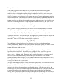
The decay of many radionuclides involves the emission of γ-rays. Processes that leave the
daughter in an excited state can lead to gamma emission. Alpha emission and beta emission
precede gamma decay in the natural radionuclides. For example, there can be a large difference
between the nuclear spin of the ground states of the parent and the daughter. Then the beta
transition directly to the ground state of the daughter is forbidden and therefore most of the
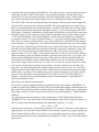
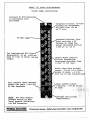
transitions leave the daughter in an excited state. Decay schemes for some radionuclides are
shown below.
60 Co
137Cs
5.26 yr
β- 0.31 MeV
57 Co
30 yr
β- 0.51 MeV
E γ = 1.17 MeV
E γ = 0.122 MeV
Eγ = 0.66 MeV
137 Ba
E γ = 1.33 MeV
60Ni
Electron Capture
E γ = 0.014 MeV
(stable)
57 Fe
(stable)
(stable)
Often the half-life of the parent is very long relative to the half-life of the daughter. In this case
gamma decay is in transient equilibrium with the decay of the parent and the γ-ray intensity falls
off with the half-life of the parent. This is the reason it is customary to name the parent as the γray source.
2-1
γ-ray spectroscopy has a number of important uses in the applied sciences. For example, it can be
used to identifying much of the elemental composition of an unknown sample. To do this the
unknown sample is irradiated with neutrons which makes the sample radio active. This is socalled ‘neutron-activation”. One can then measure the γ-rays (and β-rays) and sample half-life to
determine the constituents and their relative concentrations. This technique is used in the
petroleum industry and areas of geology, medicine, and criminology, to name a few.
To learn about γ-ray spectroscopy and standard instrumentation used in nuclear physics you will:
1. Observe γ-ray energy spectra,1
2. Identify the processes taking place,2-8
3. Complete an energy calibration of the apparatus. 9, 10
4. Determine the identity of an unknown isotope.
5. Determine the attenuation coefficients of γ-rays as a function of γ-ray energy.2, 10, 11
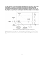
Procedure:
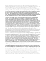
A radioactive γ-ray source is placed near a NaI(Tl) scintillation detector. The NaI(Tl) absorbs the
γ -ray and gives a light burst proportional to the amount of energy absorbed. The light is
converted into electrons by a photocathode mounted on the input of a photomultiplier tube
(PMT). The PMT is interfaced by the PMT base to a high voltage power supply and amplifier (or
preamplifier plus amplifier). The PMT outputs a current pulse which is proportional to, and
much greater than, the initial photoelectron current. Finally a multichannel analyzer (MCA)
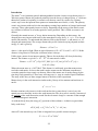
digitizes the pulses and stores a histogram of the number of pulses versus pulse amplitude. This
is shown schematically in Fig. 1.
NaI(Th)
PMT
BASE
PRE
AMP
AMP
MCA
HV
Fig. 1: Schematic drawing of the electronics for γ-ray spectroscopy. The NaI(Th)
scintillator crystal, PMT, and PMT Base are a single unit. The high voltage
applied to the base is negative and less than 1500 V. The preamp and amplifier
are typically Nuclear Instrumentation Modules (NIM) powered by a NIM crate.
The MCA is a stand alone unit.
1. Observe γ -ray energy spectra, identify the processes taking place, energy calibration the
apparatus, and determine the identity of an unknown isotope.
The UCS 30 MCA you will be using has an integral high voltage supply. Following the manual
(Appendix 3) for the MCA connect it to the high voltage input for the PMT. Using the 137Cs
source, observe the output from the anode output of the PMT base on an oscilloscope using 50
Ω termination. The pulse will be negative. Set the high voltage on the PMT so that the pulses
are > 50-100 mV. Typically ~ positive 1200 V is adequate high voltage; do not exceed +1500V.
Before continuing it is instructive to see the γ -ray line(s) directly on the oscilloscope. Each line
will appear as a brighter band. To see this you will need to get the correct trigger polarity:
negative if you take the signal from the anode output of the PMT base or positive if you take the
2-2
signal from the dynode output of the PMT base. You will also need a sweep rate that is matched
to the time response of the NaI(Tl) detector. Once you find the signal, vary the high voltage
(modestly) to see how the signal magnitude varies with applied high voltage. At this point you
may want to determine what voltage change will cause a doubling of the signal amplitude!
The UCS 30 MCA also has an integral preamp and amplifier. Following the manual (Appendix
3) for the MCA connect it to the output of the PMT. For simple applications you should set the
MCA to accumulate/display the maximum number of channels. The final choice of high voltage
and amplifier gain settings should place the highest energy γ -ray line near the upper end of the
MCA range. As different combinations of high voltage and amplifier gain will result in the same
amplitude signal you may want to investigate which combination gives you the sharpest signal:
i.e. the narrowest line for a fixed signal amplitude. At this point you should also accumulate γ ray spectra from the 60Co source to learn the range of γ -ray energies and the number of distinct
lines. Then you should consider building a cave, from lead bricks, to shield the NaI(Tl) detector
from extraneous (i.e. background) γ -rays. Where does this background come from? You should
also experiment with the distance between the source and the front of the NaI(Tl) detector. Does
this make any discernable difference other than count rate? A good rule of thumb is to place the
source at least 2 detector diameters from the detector. Why? The effective solid angle of the
detector is then (πr2)/4πd2, where r is the detector radius and d is the source-to-detector distance.
With your optimal setup you should accumulate a spectrum from each of the γ -ray sources. Do
the spectra look different from your first spectra? How and why? Do the spectra look like the
text book spectra? Identify as many of the features and lines as you can. Now take individual
spectra for a couple sources such as the 137Cs and 60Co. You may also want to try the 57Co source
if it is not too old. Do this in as short a time period as is possible. Repeat to be sure that your
peaks have not drifted! Determine the channel numbers for the center of each γ -ray line. If the
DAQ electronics and the MCA are linear there should be a linear relation between peak channel
number and γ -ray energy. To check this make a plot of channel number versus energy. Are the
points in a line? Does the curve go through (0,0) or is there an offset? To what energy does
channel 1 correspond? Now get an unknown γ source from the instructor. Using references2, 10
identify the unknown source.
Other issues you should consider include:
Do you have a circuit diagram including all equipment device types/numbers, SETTINGS, etc.
so that you could easily rebuild your setup. Have you sketched pulse shapes at different places in
the circuit? What should you check for when looking at pulse shapes? What change in phototube
high voltage results in a 100% increase in the observed γ -ray pulse heights (i.e. channel number
in MCA)?
To a first approximation the gamma ray line-width, that is its Full-Width at Half-Maximum
(FWHM) is 2.35σ, and related to the statistical fluctuations in the number of photo-electrons, Ne,
that are collected from the photocathode of the phototube. In turn Ne ∝ E , thus:
γ
σ /E = 1/√Ne ∝ 1/√E
γ
γ
2
Thus this ratio measures Ne. Check this by plotting (E /σ) versus E . If the plot is linear then our
approximation was valid; that is there should be an essentially constant γ-ray energy required per
observed photo-electron. What is the average γ-ray energy/photo-electron in your experiment?
The inverse question is how many photoelectrons result from a 1 MeV γ-ray?12 Does this number
make sense?
γ
2-3
γ
γ -ray (i.e. photon) cross sections for interacting with the NaI(Tl) are rather small in the energy
range of a few hundred keV to ~MeV. The photon interaction processes include the photoelectric
effect, Compton scattering and pair production. What photon cross section is most directly
related to the total conversion of the γ -ray to visible light in the energy range of this experiment?
Is this the dominant cross section at these energies? What is the dominant photon interaction?
Does this dominant process result in events in the observed γ -peaks? If not how do events get to
be in the peak?
2. Measure γ -ray attenuation coefficients:
Just as γ -rays interact with the NaI(Tl) to be detected or with lead shielding to reduce
background counts, γ -rays interact with all matter. The physical processes include the
photoelectric effect, Compton scattering and pair production as noted above. These cross
sections are combined (in a variety of ways depending on the precise definition) into an
absorption or attenuation coefficient, µ. Thus following a distance, X, an initial number of γ rays, N(0), is attenuated to a final number, N(X):
N(X) = N(0) e- X
µ
Because the photon cross sections change rapidly with energy and depend on the absorber
material's nuclear charge, it is interesting to measure µ at different energies and for more than
one absorber material.
To measure the energy dependence of µ, start with the 137Cs source and the MCA. To know N(0)
for each γ-ray line, you need to take (and fit) a MCA spectra with no absorber and for a known
”live-time” interval. Then take additional spectra with different thickness of absorber and for
different types of absorber. Copper and lead are available. Plot N(X,E ) versus absorber
thickness, X, as you accumulate the data. Remember to include the statistical uncertainty in each
measurement, δN, in your plot:13
γ
δN = √N
Are your statistics sufficient such that δN << N ? If not, accumulate spectra for longer periods
of time. If spectra are accumulated for different time intervals how do you record them in one
plot? Have you taken spectra for enough absorber thicknesses to measure the X-dependence of
N(X) at small-X where N(X) ~ N(0), and also at large X where N(X) << N(0). Why is this
important? Now try the 60Co source. Should your steps in absorber thickness be the same at
different γ-ray energies and/or for different absorbing materials? Why or why not?
Do you need to correct for the NaI(Tl) efficiency, ε ? Why or why not? Because you expect an
exponential decrease with absorber thickness you should plot your data on a semi-log plot. Do
your results agree with the exponential dependence on absorber thickness? Do your results agree
with smaller values for µ at larger γ-ray energies? If the answer to either of the last two questions
is no, then you may want to reconsider the geometry of your experimental setup. Can the
absorber provide a scattering path for γ-rays not initially directed at the NaI(Tl) detector to
scatter into the detector? How can you minimize this experimental problem? Once you have a
reliable experimental geometry and analysis procedures, take sufficient spectra to measure µ at
several energies and for at least two absorber materials. How do your results compare with
tabulated values for µ?
Part 2: Measurement of the Mean Life of the Muon
2-4
Introduction
The muon14 is an elementary particle indistinguishable from the electron except that its mass is ~
200 times greater. Muons are produced primarily from the decays of charged pions, π±, which are
themselves produced (copiously) in extensive air showers caused by cosmic rays. Primary
cosmic rays cover the spectrum from protons to intermediate mass nuclei (< iron). The primary
cosmic rays interact with nuclei in the atmosphere creating large numbers of charged and neutral
π mesons. These subsequently interact or decay. Depending on the energy of the initial cosmic
ray, millions or billions of secondary particles can be produced. This is called an extensive air
shower.
Generally the neutral mesons, πo, decay before interacting. Depending on their energy, the
charged pions may interact with nuclei in the atmosphere or may decay, π → µ + ν, to charged
muons and neutrinos. To understand this behavior look up the lifetimes, τ , and masses, m , of
charged and neutral pions. The average distance they travel (before decaying) depends on their
energy, E , and is given by:
±
±
π
π
π
Distance ~ (E /m c2) c t
π
π
where c is the speed of light. What are typical distances if E = 109 eV or if E = 109 eV? If this
distance is large then it is likely the π interacts before it decays.
π
π
Unlike pions, muons do not interact strongly. Thus to first order they will decay before they
interact. The distance a typical E = 109 – 1010 eV muon travels is thus:
µ
9
10
Distance = (10 ~10 [eV])/(105.7 [MeV])(3 x 108 [m/s])(2.197 x 10-6 [s]) =
6.24~62.4 [km].
Where the muon mass m = 105.7 MeV. This distance is sufficiently great that many muons
reach the earth surface. In fact at the earth's surface muons are the dominant component of
secondary particles from cosmic ray showers. Most of the muons are of modest energy by the
time they reach ground level. Thus some will range out, i.e. stop, in a tank of liquid scintillator.
The study of the decay of these stopped muons is the basis of this experiment.
µ
Muons decay via the weak interaction similar to the β-decay of free neutrons and nucleons in
nuclei:
µ± → ν + e± + νe
µ
Because neutrinos only interact via the weak nuclear force, muon decay is one of very few
natural processes that only involves the weak interaction. The decay rate is actually a measure of
the strength of the weak interaction, much like the electronic charge is a measure of the strength
of the electromagnetic interaction.
As with nuclear β-decay the energy (Ee) spectrum of the resultant e± is that for a typical three
body weak decay:1
dΓ( Ee)/dEe = (GF2/12π 3) m 2 Ee 2 (3 - 4 Ee /m ).
µ
µ
where dΓ is the muon decay rate. If this is integrated over possible electron energies:
Γ = 1/τ = GF2 m 5/192π 3
µ
µ
2-5
where τ is the muon lifetime and GF is the Fermi coupling constant. The Fermi coupling
constant is the fundamental coupling constant of the charge changing weak interaction. Thus a
measurement of the muon lifetime provides a measurement of GF once the muon mass is known!
µ
A fraction of the muons that reach the earth’s surface have just the correct energy to stop in a
block or tank of scintillator. As the muons stop they deposit ~ 2 MeV/(gm/cm2) in the
scintillator. Because the density of scintillator is ~1 (gm/cm3), muons deposit ~ 2 MeV/cm of
path length. This is much greater than the ~ 1 MeV/cm of typical γ-rays in Part 1 of this lab.
Thus these stopping muons result in a pulse of light (in the scintillator) which is easily detected.
Roughly 5% of the µ- will be captured into low Bohr orbits and then interact with the nucleus of
the scintillator atoms before decaying. Thus the majority of µ and virtually all the stopped µ+
decay before interacting with electrons or nuclei in the scintillator. Each muon decay results in
an electron with a energy up to m /2 ~ 53 MeV (i.e. neutrinos are essentially massless). These
electrons also can result in a pulse of light (in the scintillator) which is also easily detected.
−
µ
If one starts a clock each time a muon stops, i.e. this defines t = 0, then for a total of Nstop stopped
muons the number of muons remaining at a time t later is:
N(t) = Nstop exp (-t /τ ).
µ
Note: clearly this assumes that muons are not lost due to interactions with the scintillator (see
comments above). Process other than weak decays that remove muons will result in a low value
for τ . Random accidentals will be flat in time and will result in a high value for τ , unless you
analyze your data properly.
µ
µ
The number of muon decays in the time interval from t1 and t2 is:
ΔN(<t>) = N(t1) - N(t2) = Nstop {exp (-t1/τ ) - exp (-t2/τ )} ~ Nstop (Δt/τ ) exp (-<t>/τ ).
µ
µ
µ
µ
where Δt = t2 - t1 and <t> = (t2 + t1)/2, and the approximate relation is valid when Δt << τ . Thus
a histogram of the number of the observed decays, ΔN(<t>), binned in time bins of width Δt, is
predicted to be a simple exponential in <t>/τ . A semi-log plot of ΔN(<t>) versus <t> will have
a slope -1/τ .
µ
µ
µ
Procedure
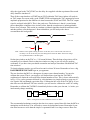
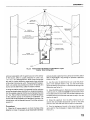
The muon decay experiment starts with a large tank of liquid scintillator viewed by two
phototubes (PMTs). If one PMT is sufficient to trigger on cosmic ray muons and on the electrons
from muon decay, why use two PMTs? The basic setup is shown schematically in Fig. 1. As
depicted in Fig. 1, the difference between a through going muon and a stopped muon followed
by a β-decay, is one pulse versus two pulses.
2-6
µ
1
BASE
PMT
µ
2
1
SCINTILLATOR
µ
1
PMT
BASE
SCOPE
ELECTRONICS
e
Fig. 1. Schematic setup for muon lifetime experiment. µ1 passes through the
scintillator losing some energy: A single voltage pulse appears on the scope. µ2
stops in the scintillator and decays after time t to an electron: Two voltage
pulses appear on the scope.
You will measure the lifetime of the muon using two different approaches for the ‘electronics’
package shown in Figure 1. The first is based upon Nuclear Instrumentation Module (NIM)
electronics. Although no longer routinely used to accumulate the final data in modern particle
physics experiments it is often still used to set up such experiments as it allows for oscilloscope
validation of each step of the experiment upon which a dedicated board can then be designed,
fabricated and used. The second method you will use to measure the muon lifetime is with just
such a dedicated board. By making the measurement using both approaches you will see the
individual measurements made in nuclear/particle physics via NIM instrumentation and how
present day experiments are conducted with dedicated boards.
1. NIM Based Measurement
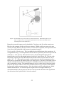
A sketch of a realistic experimental setup is shown in Fig. 2. The PMTs require negative HV
and ~ -1500 V or less should provide adequate output signals. In practice you need to adjust the
HV for each PMT to get approximately the same output signals. Typically the PMT output
signals are discriminated with Vthreshold = 30 mV. Set the discriminator output pulse length to ~ 20
ns. Are the pulse lengths sufficient to allow for the variation in pulse timing between the 2 PMTs
and still give a coincidence? Have you adjusted the relative time delay between the two
scintillator signals so the signals are in time on average? Set the coincidence unit to require a 2fold coincidence. The coincidence requires that both PMTs are above threshold to avoid noise
triggers or triggers from cosmic ray muons that are clippers.
To monitor and set up your experiment pass signals of interest through the scope; i.e. put the
oscilloscope between outputs of interest and the next device in the logic/signal chain.
MCA
BASE
PMT
SCINTILLATOR
PMT
BASE
DISCRIMINATOR
SCOPE
COINCIDENCE
CIRCUIT
DELAY
START
TAC
STOP
DISCRIMINATOR
Fig. 2. A practical experimental arrangement for the muon lifetime experiment.
Two outputs are taken from the coincidence unit. One is delayed and used to START the TAC.
The other is used to STOP the TAC. For details on how a TAC works see Appendix 1. At first
this order appears to be counter intuitive. This is explained by Fig. 3 and by the fact that only
when the TAC receives a good START-STOP combination will it produce an output pulse. To
2-7
delay the signal to the TAC START, use the delay box supplied with the experiment. How much
delay should be introduced?
Thus all the events that have a START but no STOP within the TAC time window will result in
no TAC output. For events with a good START-STOP combination the TAC output pulse has an
amplitude proportional to the difference in time between the START and STOP. The TAC output
signal is analyzed in the MCA. This is the good news. The bad news is that if a second muon
passes through the scintillator close in time to first, then the second muon is indistinguishable
from a decay electron. This results in a random accidental signal that should be uniform in time
and thus produce a flat background. Start to think how you will analyze the data to
accommodate this background!
e
µ
TO TAC START
START SIGNAL TIME
TO TAC STOP
STOP SIGNAL TIME
e
µ
DELAY TIME
FIG. 3. Sketch of the signals entering the TAC versus time (not to scale in time). The effect of
the delay is to cut off the first part of the histogram stored in the MCA. It does not change
the exponential nature of the histogram.
Set the time window on the TAC to ~ 5-10 muon lifetimes. Thus the data at large times will be
essentially all accidentals. Don't set the time window too long or you will only be studying
accidentals. If you have time you should accumulate and analyze data taken with different TAC
time windows.
To obtain adequate statistics you will need to run for at least 24 hours. Remember to leave a big
DANGER HIGH VOLTAGE sign on you apparatus.
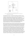
The raw data from the MCA is a histogram of counts versus channel number. You need to
calibrate the system. That is, you supply a well defined time signal into the TAC/MCA
combination to obtain the conversion from channel number to time. This is shown schematically
in Fig. 4. Use a pulse generator followed by a discriminator (or simple splitter) to create two intime signals. Put one through a precision delay. Calibrate the full scale of the TAC/MCA. If you
take data sets with different TAC time windows you will need to calibrate for each TAC setting.
Remember to calibrate the TAC/MCA immediately before or after your data run, i.e. before you
inadvertently change something.
PULSER
DIVIDER
DELAY
STOP
TAC
MCA
START
FIG. 4. Arrangement for time calibration of the TAC-MCA.
The recommended technique to analyze the data is to extract a spread sheet file from the MCA to
manipulate and fit the data. You will need to correct for background counts. Remember if your
time bins become too wide then the simple 1-exponential form is no longer correct. How does
2-8
your measurement compare with the world average of τ = 2.197 µs?15 If you agree within 5-10
% you are measuring the Fermi coupling constant to that same precision!
µ
2. Dedicated Board Based Measurement
The QuarkNet card was designed and built by engineers at Fermilab in Batavia, Illinois to
replace traditional NIM. A single circuit board amplifies PMT signals by 10x and uses voltage
comparators for discrimination with adjustable threshold. On-board timing is implemented with
CPLD (Complex Programmable Logic Device) via software installed at Fermilab. Photon events
are time-resolved with an accuracy of 1.25 ns using a time-digital-converter. A micro-controller
interfaces with the control PC using a custom LabVIEW program.
Connect the PMT outputs to two detector input channels on the QuarkNet card. Each channel
preamplifier has 50 Ω input impedance, so if the PMT signals are also being monitored on a
parallel oscilloscope the channel input impedance should be set to 1 M Ω. Apply 5 VDC power
to the QuarkNet card by plugging the AC adapter into a wall socket. A blinking LED associated
with each channel indicates the occurrence of a local trigger. The LEDs can give a rough visual
guide to assist in configuration (Note: the digital counter is of little value). Open the LabVIEW
program Setup.vi.
Card Timing: Triggering can be initiated by either: 1) one pulse from a single PMT or 2)
coincident pulses from 2, 3, or 4 PMTs. Coincident triggering is more reliable because it is less
susceptible to false signals produced by random background noise. This experiment has two
PMTs available to monitor photons in the scintillator tank.
If coincident triggering is used, the time overlap window (coincidence time) must be set. The
default value is 40 ns. At the default setting, two PMTs must produce individual pulses that
exceed their specified threshold voltage AND occur within 40 ns of each other to create a trigger.
If the coincidence time is too short, relatively few card triggers will occur. If it is too long, there
is increased probability of false triggers. The oscilloscope display of the pulses can guide this
setting. The coincidence time has no meaning in the single trigger configuration.
Once the card triggers, all the detector input channels will record above-threshold photon signals
during a specified time (gate width). The proper gate width will depend on the type of
experiment being performed. If only the triggering pulse or pulses are to be recorded, the gate
width can be relatively short. If muon decay events are of interest, the gate width must exceed
the expected muon lifetime by 4 to 5x. Longer than this will introduce noise; a significantly
shorter gate will make determination of the decay time difficult.
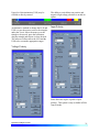
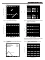
Threshold: Each channel of the QuarkNet card will
locally trigger when the amplified PMT pulse exceeds a
specified threshold voltage. This is illustrated by the
dotted red line in the adjacent figure. Recall that the
threshold voltage must be adjusted by 10x compared to
the PMT output to account for amplification on the card.
Also note that individual channel triggers do not
guarantee the gate will open if coincidence triggering has
2-9
been selected. Simultaneous PMT events as defined by the coincidence time window are
required.
The time-over-threshold of an individual pulse can be recorded with a precision of 1.25 ns. This
time gives an approximate measure of the integrated power and hence the relative energy in the
PMT pulses.
Setup: The LabVIEW program Setup.vi helps configure the QuarkNet card. The goal is to set
the PMT bias voltage along with the channel thresholds to acquire reliable data counts. The
negative-going voltage of the PMT output pulses must be sufficiently above the background
noise and at a level where they can be readily discriminated.
Initial setup should be performed with single detection, a gate width of 100 ns, and 100 mV
threshold. Negative voltage for all PMT signals is assumed, so the threshold is entered as a
positive number. These settings are not critical, but should be a good starting point. The
sampling period should be long enough that the count does not vary widely between display
updates. Start the program, wait three seconds for the card to initialize, and press the RUN
button. Detector counts will be displayed. To change an operating parameter, press PAUSE,
make the desired change, then press RUN. The PAUSE button allows parameters to be modified
without a complete card reset. As the threshold voltage increases, the count rate should drop.
When higher thresholds do not noticeably reduce the count rate, a good operating threshold
voltage is identified. Keep the PMT voltage constant and configure the second channel using the
same criteria. If adequate thresholds can't be established on both channels, the PMT voltage must
be changed.
Select the coincidence tab to enable single counting from both PMTs and display their
coincidence counts. Both detectors should be counting at a higher rate than the coincidence
events; you can also determine which of the two detectors is limiting the coincidence trigger rate.
Proper behavior verifies the threshold settings and the width of the coincidence time window.
Record the working parameters and do not adjust the PMT voltage.
Open the LabVIEW program Muon.vi. With appropriate timing settings and threshold
parameters determined above, this program records photon events collected by the PMTs. Two
measurements can be performed: photon energy distribution and muon decay lifetime.
Energy distribution: Select the measurement 'Energy' and open the Coincidence tab. The
experiment can be done with a single PMT, but more reliable data is obtained with simultaneous
signals from two PMTs to verify the presence of a valid photon in the scintillator. The goal of
this measurement is to determine the approximate energy of each photon event by recording its
time above threshold, shown as T in the above figure. The gate width can be set with the aid of
the oscilloscope. It should be long enough to capture the photon signal; too long will introduce
unnecessary noise. Since the width of the triggering photon is of interest, the gate minimum
should be set to zero. Only data from one of the PMTs (decay detector) will be recorded.
Start the program and wait 3 seconds for the card to initialize. When the card is ready, press the
RUN button. You will be prompted to specify the name and location of a data file where the
2-10
collected values of T (in ns) will be written. Since data can be collected for an arbitrarily long
time, this file will auto-save at a user-specified interval. Real-time data is displayed on an
updating histogram. The distribution should approach an ideal Gaussian depending on the
number of data points and histogram bins.
When sufficient data has been collected, stop the program. Repeat the measurement but stop it
when the number of data points is about half of the first run. Change the decay detector to the
other PMT and do the same pair of measurements (4 total). For the analysis, produce a histogram
with a Gaussian fit for all the data sets to determine the mean pulse width and variance; express
the latter as a percentage of the mean. How does the analysis depend on the number of histogram
bins? Comment on the differences and calculate the experimental uncertainty for each data set.
Muon decay: Select the measurement 'Decay' and open the Coincidence tab. In this experiment,
the decay detector waits for a second photon that follows the coincidence trigger, which should
correspond to a muon decay. The program must be configured to ignore trigger events, which
will radically skew the data toward time zero. The gate minimum setting must be set longer than
duration of any possible trigger pulse, accounting for fluctuations introduced by the coincidence
time window. (Tip: The gate minimum should be longer than the gate width used in the
preceding experiment) To observe the expected exponential decay, the gate should remain open
for several muon decay lifetimes (order of microseconds). If the gate width is set longer than 5
muon lifetimes, data accumulated at long times will represent the noise background. The
background data introduces a constant offset on the statistics that can be subtracted. The desired
decay events are statistically rare, so an hour or more may be needed to accumulate a useful data
set. When sufficient data is collected, stop the program. The time events are all written to the
specified data file. For the analysis, setup an appropriate histogram on a semi-log plot. The slope
of the linear fit is the measured muon decay lifetime. Calculate the experimental uncertainty and
compare the lifetime to the accepted value.
2-11
REFERENCES
1. a. W.R. Leo, Techniques for Nuclear and Particle Physics Experiments, 2nd Ed. (Springer
Verlag, New York, 1993) Ch 1.
1. b. C.M. Lederer and V.S. Shirley, Table of Isotopes, 7th Ed. (Wiley, New York, 1978).
2. W.R. Leo, Ch. 2 - Sect 2.7, Interaction of Photons with Matter.
3. W.R. Leo, Ch. 7, Scintillation Detectors.
4. W.R. Leo, Ch. 8, PMTs.
5. W.R. Leo, Ch. 9 - Sect 9.7, Scintillation Detector Operation.
6. W.R. Leo, Ch. 11, Pulse Signals.
7. W.R. Leo, Ch. 12, NIM Electronics.
8. W.R. Leo, Ch. 14, Pulse Signal Shaping and MCAs.
9. W.R. Leo, Ch. 15, Pulse Height Spectra and MCAs.
10. See Appendix 2, AN34 - Experiments in Nuclear Science, 3rd Ed.(EG&G ORTEC, 1984).
11. G.F. Knoll, Radiation Detection and Measurement, Ch. 2, 2nd Ed. (Wiley, New York, 1989).
12. Harshaw Radiation Detectors, Harshaw/Filtrol, 6801 Cochran Rd., Solon, Ohio report
FWHM/Eγ ~ 7-9 % at 662 KeV for NaI(Tl) detectors.
13. W.R. Leo, Ch. 4, Statistics and Error Analysis.
14. F. Halzen and A.D. Martin, Quarks and Leptons: an Introductory Course in Modern Particle
Physics, (Wiley, New York, 1984).
15. Particle Data Group, Phys Rev. D 54, 1 (1996)
2-12
APPENDIX 1: Time-to-Amplitude Converters
Bill Miller and Paul Schwoebel
A Time-to-Amplitude Converter (TAC) is a device that accepts a start pulse and waits for a stop
pulse. Circuitry inside the TAC determines how much time has elapsed between the two pulses.
The TAC produces a voltage pulse with an amplitude that is proportional to the elapsed time.
To use the TAC:
1. Check if there are any special power requirements like ±6 V. This can usually be found on the
front panel. Some units have a rear panel switch that allows for either ±12 V of ±6 V. Make sure
that your NIM bin has correct voltages available.
2) Check to see what logic family the unit uses, NIM logic (a "V" looking character) or TTL (a
representation of a positive going pulse). Some units can be switched between the logics.
3) Set up the TAC for the proper time scale. If you set it up for a 1 µs scale and give it a signal
with 2 µs between start and stop you will not get an output from the TAC. Similarly, If you
select 1 µs and deliver only 1 ns the TAC will provide no output.
4) There can be a number of extra functions on the front panel. For COINC and ANTICOINC
select ANTICOINC. GATE should be OPEN. The SCA is not important for this experiment.
Leave the ULD at 10 and the LLD at 0. Buttons or switches associated with the SCA should be
set to OFF or OUT. Anything that says DELAY is not important. This adjusts the time between
the accepted STOP signal and the TAC output pulse. For slow count rates, 10 µs is nothing to
worry about.
2-13
APPENDIX 2: Gamma-Ray Spectroscopy
EG&G ORTEC
Wednesday, December 11, 2002
ORTEC AN34 Experiments in Nuclear Science Laboratory Manual
Page: 1
AN34
Application Note
Experiments in Nuclear Science
AN34
Laboratory Manual Third Edition, Revised
Introduction to Theory and Basic Applications
Alpha, Beta, Gamma, X-Ray, and Neutron
Detectors and Associated Electronics
Published September 1987.
http://www.ortec-online.com/application-notes/an34/an34-front.htm
APPENDIX 3: MANUALS
UCS 30
Universal Computer
Spectrometer (USB)
Quick Start Guide
April 2008
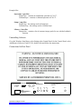
IMPORTANT NOTE
Software for this spectrometer should be installed before it is
connected and powered on. If you have already connected the
UCS 30 to your computer, do not power on until software installation is complete.
Spectrum Techniques, LLC.
Oak Ridge, Tennessee USA.
INTRODUCTION
The purpose of this guide is to provide you with assistance to quickly install, setup, and begin using
your UCS 30 Universal Computer Spectrometer (USB).
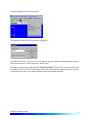
INSTALL SOFTWARE
Install the software CD shipped with your UCS 30 system into your CD ROM drive. The auto-start
feature will open the InstallShield Wizard. Click Next to continue.
Verify your user information and the default destination folder C:\Program Files\Spectrum Techniques\UCS30\.
You might want to note this Program installation path in case you want to store spectra in this location.
UCS 30 Quick Start Guide
2
Click Install to begin program installation if you are satisfied with your entries.
The installation will begin. You can monitor the install progress by watching the status bar. The install should be reasonably quick and will conclude by displaying the InstallShield Wizard Completed screen. Click Finish to exit the install wizard.
Note the UCS 30 icon that has been installed on your desktop.
Using your Windows Explorer, examine the contents of C:\Program Files\Spectrum Techniques
\UCS30\ . This file should contain a Drivers folder, an Examples folder, and several UCS 30 files
including the UCS 30 Manual in Adobe PDF format. You may want to create a shortcut to the manual and place it on your desktop for quick reference.
Remove the installation CD from the CD ROM drive and store it in a safe place.
SYSTEM SETUP
Connect your detector to the UCS 30. Connect the detector high voltage cable to the MHV connector on the UCS 30 labeled POS HIGH VOLTAGE.
Connect the BNC signal cable from the detector to the BNC connector on the UCS 30 labeled INPUT.
NOTE: If you are using a detector with a preamplifier included, connect to the INPUT BNC connector and set the UCS 30 MODE to PHA (Amp In).
If you are using a detector with a preamplifier AND external amplifier, connect the detector signal cable to the INPUT BNC connector on the UCS 30 and set the MODE to PHA (Direct In).
Turn on the power to the UCS 30.
Your PC should detect the presence of a new hardware device and may automatically install the required software. If the software does not load automatically, follow the system prompts. Remember,
the location of the software is C:\Program Files\Spectrum Techniques\UCS30\ .
UCS 30 Quick Start Guide
3
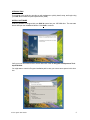
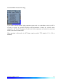
After you specify location of your software, you may see the following screen, or similar:
Select Continue Anyway and finish the installation.
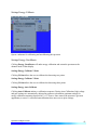
Start the UCS 30 program by double-clicking on the UCS 30 icon on your desktop.
Place a Cs-137 calibration source on your detector.
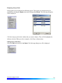
Next, open the Settings pull-down menu. Click on Energy Calibrate, then select Auto Calibrate.
The system will now auto calibrate. This process will take several minutes. Once completed, the
message box will display the current settings for high voltage, coarse and fine gain. The screen is
now energy calibrated from 0 to 1024 KeV.
Erase spectrum using the eraser icon.
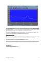
Click the Go button and take a spectrum until you obtain a well defined peak at the 662 keV line of
Cesium. Stop the acquisition.
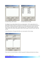
Set the ROI by clicking on Settings, ROIs, then Set ROI. Place the cursor over the lower channel
you wish to start the ROI with, hold down the left mouse key and drag the cursor to the desired upper
channel for the ROI. Release the mouse button and the ROI will be set and highlighted. When the
cursor is placed anywhere in the ROI, the total counts in the ROI will be displayed.
UCS 30 Quick Start Guide
4
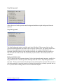
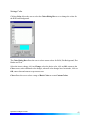
Now set a preset count. You can choose Time, then Real Time or Live Time, or Integral Counts.
Let’s use Integral Counts since we have set a Region of Interest (ROI). Select Settings, Presets,
then Integral Counts. In the box, enter a number for the desired level of counts in the ROI that will
stop data acquisition. (Note: You must first have your cursor set in your ROI.)
Click on File and Save Setup, enter a file name and save. You can use this count protocol whenever you wish by selecting File, Load Setup and selecting this file.
USING YOUR SYSTEM
This guide is intended to help you setup and begin using your UCS 30 as quickly and easily as possible. The more you use the system, the more you will become familiar with its operation.
More detail on operation is provided in the UCS 30 user’s manual.
Contact us if you still have questions, comments or problems pertaining to your system or its operation.
Spectrum Techniques
(865) 482-9937
http://www.spectrumtechniques.com
UCS 30 Quick Start Guide
5
Spectrum Techniques
UCS-30
Universal Computer Spectrometer
SPECTRUM TECHNIQUES, LLC.
106 Union Valley Road
Oak Ridge, TN 37830
USA
Telephone (865) 482-9937
Fax (865) 483-0473
e-mail: [email protected]
Web Site: http://www.SpectrumTechniques.com/
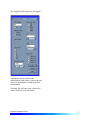
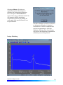
Introduction ............................................................................................................................... 5
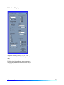
Screen View .................................................................................................................. 7
Installation................................................................................................................................. 7
Installing Software ........................................................................................................ 7
Uninstalling Software ................................................................................................... 8
Connections On Rear Panel .......................................................................................... 8
Analysis Modes........................................................................................................................10
Pulse Height Analysis (PreAmp In) .............................................................................10
Pulse Height Analysis (Amp In) ..................................................................................10
Pulse Height Analysis (Direct In) ................................................................................10
Multi Channel Scaling (Internal) .................................................................................11
External Multi Channel Scaling ...................................................................................13
Mossbauer (Internal) ....................................................................................................14
Mossbauer (External) ...................................................................................................15
Operation..................................................................................................................................16
Live Mode ....................................................................................................................16
File Mode .....................................................................................................................16
Amp/HV/ADV .............................................................................................................16
Configuring System Parameters ..............................................................................................18
High Voltage ................................................................................................................18
Amplifier Coarse Gain .................................................................................................19
Amplifier Fine Gain .....................................................................................................19
ADC Conversion Gain .................................................................................................20
Lower and Upper Level Discriminators ......................................................................20
Voltage Polarity ...........................................................................................................21
Input Polarity ...............................................................................................................21
Peak Time Shaping ......................................................................................................22
Presets ..........................................................................................................................23
Preset Time ......................................................................................................23
Preset Integral ..................................................................................................24
Go, Stop and Erase .......................................................................................................24
Regions of Interest (ROI).............................................................................................24
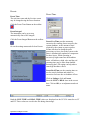
Functions ..................................................................................................................................25
Energy Calibration .......................................................................................................25
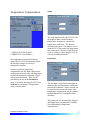
Temperature Compensation .........................................................................................27
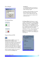
Isotope Matching .........................................................................................................28
Strip Background .........................................................................................................31
Load Spectrum .................................................................................................32
Load Background .............................................................................................32
Show Spectrum ................................................................................................32
Show Background ............................................................................................32
Overlay Spectra ................................................................................................33
Strip Background from Spectrum ....................................................................33
Data Smoothing ...........................................................................................................34
Menu Bar .................................................................................................................................34
File ...............................................................................................................................34
Spectrum Techniques UCS-30
2
File Open ..........................................................................................................35
File Save...........................................................................................................35
File Load Setup ................................................................................................35
File Save Setup ................................................................................................35
File Load Library .............................................................................................35
File Save Library..............................................................................................35
File Print...........................................................................................................35
File Print Preview ............................................................................................35
File Print Setup ................................................................................................36
File Exit ............................................................................................................36
Edit ...............................................................................................................................36
Edit Experiment ...............................................................................................36
Edit Iso Match ..................................................................................................36
Edit Smooth Data .............................................................................................38
Mode ............................................................................................................................38
Display .........................................................................................................................38
Display Peak Report ........................................................................................38
Display Data Report .........................................................................................39
Display Calibration ..........................................................................................39
Display ROIs....................................................................................................39
Display Iso Match ............................................................................................39
Display Pixel Sizes ..........................................................................................39
Settings.........................................................................................................................40
Settings ROIs ...................................................................................................40
Settings Energy Calibrate ................................................................................41
Settings Preset ..................................................................................................42
Settings Amp/HV/ADC ...................................................................................42
Settings MCS ...................................................................................................42
Settings Color...................................................................................................43
Settings Confirm Spectrum Erasure.................................................................44
Settings Reset All Variables To Defaults ........................................................45
Strip Background .........................................................................................................45
Strip Background – Load Spectrum.................................................................46
Strip Background – Load Background ............................................................46
Strip Background – Show Spectrum ................................................................46
Strip Background – Show Background............................................................46
Strip Background – Overlay Spectrum ............................................................47
Strip Background – Strip Background from Spectrum ....................................47
View .............................................................................................................................48
Tool Bar ...........................................................................................................48
Status Bar .........................................................................................................48
Help ..............................................................................................................................48
Contents ...........................................................................................................48
Using Help .......................................................................................................48
About................................................................................................................48
Tool Bar ...................................................................................................................................49
Spectrum Techniques UCS-30
3
Go.................................................................................................................................49
Stop ..............................................................................................................................49
Erase .............................................................................................................................50
Show Peak Report ........................................................................................................50
Show Data Report ........................................................................................................50
Amp/HV/ADC .............................................................................................................50
Presets ..........................................................................................................................50
ROI ...............................................................................................................................50
Spectrum Window Sizing ............................................................................................50
X axis expand ...................................................................................................51
X axis contract .................................................................................................51
Specifications ...........................................................................................................................52
Hardware ......................................................................................................................52
Software .......................................................................................................................53
Spectrum Techniques Contact .................................................................................................53
Spectrum Techniques UCS-30
4
Introduction
Hardware
The Universal Computer Spectrometer offers a unique solution for nuclear spectrometry using
the PC platform. A 4K ADC (optional) combined with 8K of data memory and multi-channel
scaling is ideally suited to scintillation spectroscopy and time related studies such as half-life
decay.
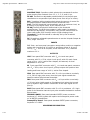
Constructed in a sturdy, fully-shielded bench top enclosure with Universal Serial Bus (USB)
computer interface, the multi-channel analyzer contains many advanced features including
computer controlled amplifier and high voltage for PM tubes, upper- and lower-level
discriminators, on-instrument data memory, and a comprehensive software package for use
under Windows 2000 or higher.
The UCS-30 requires only an available USB port and is designed to work seamlessly with USBequipped PCs. For stability and low noise operation, the unit is AC-line powered with an autosensing power supply for 100-250 VAC operation. An on-board microprocessor acts as the
master controller and data storage device, as well as the communication link directly to the USB
interface.
The integrated amplifier and high voltage are fully compatible with most standard scintillation
detectors, eliminating the need for special tube bases and external modules. For ease of setup and
calibration, coarse gain, fine gain, high voltage, and lower- and upper-level discriminator settings
are controlled directly from the desktop computer. For operation with other types of detector
systems such as alpha spectrometers or single photon counting, the scintillation preamp and
amplifier can be bypassed (by computer control while in the “Mode” menu) which allows direct
access to the ADC.
A 4096 channel ADC with de-randomizing buffer offers excellent data throughput at high
counting rates with minimal dead-time losses. Conversion gain may be changed from 4096 to
either 2048, 1024, 512, or 256 channels via the software. Data from the ADC is stored directly in
on-board memory for autonomy and high-speed operation, freeing the host computer for other
tasks.
Software
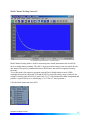
The UCS-30 produces a high-resolution, real-time live color display of spectral data with
standard PC graphics running under Windows® (2000 and above). Operation is intuitive using
pull-down menus and function buttons for the most commonly used commands and display
options. The software offers full control of all features including preset live/real time and
regions-of-interest, together with centroid, gross and net area calculations.
Control of the hardware amplifier, high voltage, ADC and input discriminators is also through
function buttons for straightforward calibration and operation. To simplify identification of
Spectrum Techniques UCS-30
5
peaks, the cursor may be calibrated to read directly in energy units, using either a 2-point linear,
or 3-point quadratic relationship calibration to allow for detector non-linearity.
Spectral files may be transferred to disk for long-term storage as binary files or transferred
through the clipboard in ASCII format for exporting to other programs. Stored files may be used
to collect background data over a long counting period that can be subtracted on a time
proportional basis from the spectral data.
To aid in the identification of nuclides, the UCS-30 contains a unique peak-labeling feature
named ISOMATCH. Providing the unit is accurately energy calibrated, the user may select a
nuclide from the library and the corresponding characteristic emission lines are superimposed on
the spectrum along with isotope and energy information. Using this feature, users may quickly
check a spectrum and visually identify the emission components for each nuclide present. The
ISOMATCH libraries may be created or customized using a text editor.
When operating in multi-channel scaling mode, the system may be calibrated in time units for
direct readout from the cursor.
Both linear- and logarithmic-vertical display ranges are included, which can be useful when
performing decay studies
Spectrum files can be transferred from the ICS 10 DOS program and the ICSW 16
Windows program to the UCS-30 Windows version format.
Most functions may be accessed by more than one method. All the functions can be accessed
from the Pull Down Menues, some from the Tool Bar Buttons, or by the mouse. If the function
has a Tool Bar Button, its symbol will be shown on the left-hand side of the description.
Spectrum Techniques UCS-30
6
Screen View
Installation
System Requirements
The UCS-30 instrument uses a Universal Serial Bus (USB) to communicate with a PC. The PC
must have USB compatible drivers, which are available standard on Windows 2000 and later
releases. The performance of the USB on older systems may affect the perceived performance of
the software; so we recommend that you use a Pentium III or greater class of microprocessor
running at 550 MHz or greater to achieve desirable performance.
Installing Software
Insert the included CD in your CD-ROM drive. The install program will automatically run.
Follow the instructions to select the options you want to install.
The default installation directory is C:\Program Files\Spectrum Techniques\UCS 30
Spectrum Techniques UCS-30
7
Example files:
Spectrum (*.spu) files:
Normal.spu – contains an uncalibrated spectrum of CS-137.
Calibrated.spu – contains a calibrated spectrum of CS-137.
Setup (*.sup) files:
Normal.sup – has settings used in Normal.spu.
Calibrated.sup – has settings used in Calibrated.spu.
Library (*.itm) files
Isotopes.itm – contains a list of common isotope peaks for use with the IsoMatch
function.
Uninstalling Software
Go to the Windows Start Menu, select Settings, then Control Panel. On the Control Panel, select
Add/Remove Software. Find UCS-30, double click and follow the instructions.
Connections On Rear Panel
PREAMP POWER
AC POWER IN
90 — 240 VAC
50 — 60HZ
POS
NEG
WARN ING:
DANGEROUS VOLTAGES
ON HV CON NECTORS
MANUFACTURED BY SPEC TRUM TECHNIQUES
OAK RIDGE TENNESSEE 37830
MADE IN USA
HIGH VOLTAGE
USB
MSB
OUT
ROI
OUT
GATE
IN
MCS
IN
T/COMP
INPUT
WARNING:
DANGEROUS VOLTAGES INSIDE
SERVICE BY AUTHORIZED
PERSONNEL ONLY
Rear Panel
Spectrum Techniques UCS-30
8
CAUTION: Be sure to use the correct high voltage polarity for your device to prevent
possible damage to equipment.
POS HIGH VOLTAGE: MHV (or optional SHV) connector supplies positive 0 - 2048 volt
@ 1mA maximum current to power scintillation detectors. High voltage is fully regulated and
computer controlled in 2 volt increments.
NEG HIGH VOLTAGE: Negative High Voltage is an Option. If this option is added, the
UCS30 can also supply negative 0 - 2048 volt @ 1mA maximum current to power scintillation
detector through an MHV (or optional SHV) connector. High voltage is fully regulated and
computer controlled in 2 volt increments.
Either the POS HIGH VOLTAGE or NEG HIGH VOLTAGE may be selected for use. Go to
the “Settings” menu, then choose the “Amp/HV/ADC Settings” sub menu to gain access to the
polarity selection.
WARNING: HIGH VOLTAGE must be “OFF” before switching between POS HIGH
VOLTAGE or NEG HIGH VOLTAGE. Failure to comply with this WARNING may result in
severe instrument damage.
INPUT: BNC connector. This input is for signals from a scintillation detector, scintillation
preamplifier, or other type detector amplifiers (proportional counter, germanium detector) for
eventual processing by the ADC. The internal scintillation preamplifier and also the scintillation
amplifier can be bypassed using the “Mode” menu.
MCS IN: BNC connector to input positive Multichannel Scaling (MCS) TTL pulses, > 150nsec.
5 MHz maximum rate.
ROI OUT: (OPTIONAL) BNC connector supplies a pulse output when data is acquired in a
channel marked as a Region of Interest (ROI). The pulse width is adjustable from 100 sec to 25
msec by an internal pot. The pulse amplitude is adjustable from 0 volt to 7.5 volts by an internal
pot.
GATE IN: BNC connector for connection to external coincidence unit. A positive TTL pulse
causes the ADC to accept the next pulse. The Gate pulse must be present before the peak of the
input Pulse. Gate pulse width = 50 nsec to 2 sec.
MSB OUT: BNC connector to output the most significant MCS bit for Mossbauer Applications.
The output pulse period in seconds is equal to the dwell time multiplied by the conversion gain.
Used as a trigger for an external device (i.e. constant acceleration drive). Output will begin after
the first pass in Mossbauer mode.
T/COMP: Modular connector for connection to temperature compensated tube base.
USB: Universal Serial Bus connector for communication with computer.
PREAMP POWER: DB-9 connector, supplies 12v power for External preamplifier.
Spectrum Techniques UCS-30
9
(NOTE: An OPTIONAL 24v preamplifier power output is available to ensure compatiblity
with germanium detectors.)
Analysis Modes
Pulse Height Analysis (PreAmp In)
Similar to the 'PHA PreAmp In' operating
mode except that the incoming signal
bypasses the instrument's internal PreAmplifier.
The amplitude of each detector pulse is
measured by the ADC and stored as an
amplitude (energy) spectrum.
This is the normal operating mode for
collecting sample gamma emission spectra.
The amplitude of each detector pulse is
measured by the ADC and stored as an
amplitude (energy) spectrum.
The X axis is scaled to the selected channels
and the Y axis is scaled for the counts for each
channel. Y axis counts that exceed the
maximum Y axis value are ‘wrapped’; they no
longer are scaled to the Y axis, and they
appear in a different color.
Pulse Height Analysis (Amp In)
Pulse Height Analysis (Direct In)
Similar to the 'PHA PreAmp In' operating
mode except that the incoming signal
bypasses both the instrument's internal PreAmplifier and Amplifier.
The amplitude of each detector pulse is
measured by the ADC and stored as an
amplitude (energy) spectrum.
Spectrum Techniques UCS-30
10
Multi Channel Scaling (Internal)
(UCS20 MCS Spectrum shown; UCS30 similar)
Multi Channel Scaling mode is used for measuring time related phenomena such as half-life
decay or single photon counting. The ADC is bypassed and incoming events are routed directly
into memory for specific predetermined times (dwell time) and stored in sequential memory
locations.
To use this mode, first acquire a spectrum using the Pulse Height Analysis mode. While
acquiring the spectrum, adjust the LLD and the ULD to select the energy range of interest (for
example, selecting only the 662 keV peak from CS-137 will eliminate unwanted background and
produce a superior decay curve when using a Cs-137/Ba-137 mini-generator.)
Click the Mode menu and select MCS
Spectrum Techniques UCS-30
11
Click the Settings menu and select MCS
The Setup MCS Dwell Time dialog box will appear:
Enter the Dwell Time. This time is for each memory location (channel). Remember the total pass
time will be equal to (Conversion Gain x Dwell Time).
Erase any current memory data and click START COUNTS. The UCS-30 will proceed to count
incoming events for the selected dwell time, store the total in the first channel location, reset the
counter and repeat the cycle storing each total count in sequential channels.
Spectrum Techniques UCS-30
12
External Multi Channel Scaling
If you wish to use an external pulse generation system such as a coincidence circuit, it will be
necessary to bypass the on-board amplifier and discriminators. Connect the external counts
connector to the Ext MCS connector on the back of the instrument and select the menu item
MODE, then select External MCS.
When operating in this mode, the MCS input requires positive TTL signals (>2.5v, >150 ns
duration).
Spectrum Techniques UCS-30
13
Mossbauer (Internal)
This mode uses the internal preamp. Connect the signal into the INPUT BNC connector. The
Mossbauer mode has variable dwell time ranging from 100 Sec to 6 Sec. A Preset number of
passes can be set to the desired number or left at zero (0) for infinite passes.
The following is the Mossbauer spectrum of a Co-57 source with an enriched Fe-57 absorber,
showing nuclear Zeeman splitting.
Spectrum Techniques UCS-30
14
Mossbauer (External)
This mode requires the use of an external amplifier. The signal must connect to the MCS
INPUT BNC connector. The Mossbauer External mode has variable dwell time ranging from
100 Sec to 6 Sec. A Preset number of passes can be set to the desired number or left at zero (0)
for infinite passes.
The following is the Mossbauer spectrum of a Co-57 source with an enriched Fe-57 absorber,
showing nuclear Zeeman splitting.
Spectrum Techniques UCS-30
15
Operation
Live Mode
instrument and is used only to view and
manipulate files that have been saved to disk.
File Mode
The software starts up in the Live Mode. This
mode uses the USB to communicate with the
instrument.
If you access the File Menu and click on
Open, a new window appears which looks like
the current window, except that the title bar
shows ‘File Mode’ instead of ‘Live Mode’.
File mode does not communicate with the
File Mode is accessible from the live mode by
going to the File Menu and clicking on Open.
Select the file you want to view. Some
functions, which have no use when viewing
files, are disabled in the Menus and the
Toolbar.
Amp/HV/ADC
Click the Amp/HV/ADC Button on the
toolbar:
Or use the settings menu and click on
Amp/HV/ADC
Spectrum Techniques UCS-30
16
The Amp/HV/ADC dialog box will appear.
Adjustments may be made to the
amplification, high voltage, conversion gain,
low level discriminator, and the high level
discriminator.
Selecting OK will cause these values to be
written to the UCS-30 instrument.
Spectrum Techniques UCS-30
17
Configuring System
Parameters:
High Voltage
Once the program is running it will be
necessary to configure the system parameters
for correct operation and calibration.
Place a gamma emitting check source near the
detector face. Cesium-137 (Cs-137) is a good
choice. It has a single peak at 662 keV.
Click on Settings, then click on
Amp/HV/ADC
Set the high voltage to the voltage as listed by
the detector manufacturer. As an example, set
the high voltage to positive 600 volts; click
ON.
DO NOT exceed the maximum high voltage
rating of the detector, usually 1200 volts.
Set the amplifier COARSE GAIN to 8, and
set the FINE GAIN to 1 as a starting position.
Click on OK, to set adjustments and exit the
menu.
Start the data acquisition and adjust the
amplifier gain until the 662 keV peak is
approximately mid-scale.
Once the acquisition is started, you may enter
the Amp/HV/ADC menu and make
adjustments while viewing the spectrum. This
will allow you to position the peak in the
desired channels.
Spectrum Techniques UCS-30
High Voltage may be entered directly in the
text box or may be scrolled to the value
desired. A warning will be issued if you
attempt to input a value higher than 1200
volts, since this is the highest value that many
probes can tolerate without damage. If you
know that your probe can accept higher than
1200 volts, you may increase the voltage up to
2048 volts.
18
Amplifier Coarse Gain
Amplifier Fine Gain
Amplifier coarse gain may be set by clicking
the radio-button next to the desired multiplier.
Amplifier fine gain may be directly entered as
a multiplier value between 1.0 and 2.275 in
0.005 increments.
Spectrum Techniques UCS-30
19
ADC Conversion Gain
Lower and Upper Level Discriminators
Conversion Gain represents the number of
channels that will be sampled and displayed
on the screen. Smaller values save as smaller
files
LLD and ULD, Lower Level Discriminator,
and Upper Level Discriminator, allow the user
to set a value between 0 and 102.3 (roughly
percent) that cuts off the input signal before it
gets to the ADC. The LLD is often used to
block high-count signals (noise) in the low
range that are not of interest, but require
excessive time to sample. The ULD may be
set up to 102.3.
The conversion gain default setting is
maximum channels. This is preferred for most
scintillation detector applications and
generally no adjustment is required.
For certain applications, such as alpha
spectroscopy, it may be necessary to change
this parameter to either 256, 512, 1024, 2048
or 4096 channels.
Spectrum Techniques UCS-30
Low level discrimination (LLD) may be
scrolled or directly entered.
20
Upper level discrimination (ULD) may be
scrolled or directly entered.
The ability to switch between positive and
negative high voltage polarities is an add-on
option.
An alternative method to change the LLD and
ULD is to use the mouse to move the triangles
under the X axis. Move the mouse over the
triangle to be moved, press the left button,
drag the triangle and release it where desired.
The software will not allow the LLD and the
ULD to be set outside appropriate ranges.
Input Polarity
Voltage Polarity
Some detectors require a positive input
polarity. This option is only available in PHA
Amp In mode.
Spectrum Techniques UCS-30
21
Peak Time Shaping
Amplifier Peaking Times of 1, 2, 4, or 8
microseconds are selectable in Amp In mode
only.
Peaking times longer than 1 microsecond are
useful with solid state detectors such as Ge(Li)
or HPGE detectors.
Spectrum Techniques UCS-30
22
Presets
Preset Time
Preset Time
The real time count and the live time count
may be changed using the Preset function.
Click the Preset Time Button on the toolbar:
Preset Integral
The instrument can be set to stop
automatically after a ROI integral.
Click the Preset Integral Button on the toolbar:
Or use the settings menu and click on Presets:
Preset Live Time provides automatic
correction for counting losses caused by the
system deadtime, or the amount of time
required by the system to process pulses.
Events which occur during the pulse
processing cycle are lost to the system so the
timer is automatically updated to compensate
for these losses. When operating at
excessively high count-rates the deadtime
meter will indicate a high value and the real
counting time may be more than doubled.
Increasing the LLD setting can help reduce
some high deadtime effects.
Preset Real Time sets the counting timer to
run for actual clocktime and makes no
correction for losses due to deadtime effects.
Click on Settings, click on Presets
Enter the LIVE or REAL time in the correct
box. Click on OK, to set adjustment and exit
menu.
Both the LIVE TIME and REAL TIME values are displayed on the UCS-30 status bar as LT
and RT. These values are saved in the file during data storage.
Spectrum Techniques UCS-30
23
Preset Integral
Set Integral
To set an integral count it is necessary to
first establish a ROI and then position the
marker within the region.
Selecting an ROI and setting a value other
than 0 in preset integral will cause the
system to STOP counting when the total
counts of all the channels within the ROI
reaches that value.
Go, Stop and Erase
Go, Stop and Erase functions are accessed
with the Tool Bar buttons. Clicking on Start
begins data collection. Clicking on Stop ends
data collection. Clicking on Erase sets each
channel’s data to zero. Additionally, three 'hot
key' combination are defined as shortcuts for
data acquisition functions. Pressing the
appropriate action key while pressing the 'Ctrl'
and 'Shift' keys will provide Go, Stop and
Erase action. To Go press 'Ctrl+Shift+A'; to
Stop press 'Ctrl+Shift+S'; and to Erase press
'Ctrl+Shift+E'.
Region of Interest (ROI)
Region of interest (ROI) selection is an
advanced feature which provides
instantaneous computation of peak gross and
net counts. These values may be used along
with isotope decay tables and detection
efficiency to calculate absolute or relative
isotopic activities. ROIs must not overlap and
need to be separated by at least one channel
for correct area calculation. Up to 16 different
ROIs are possible using the color selector
from the pull down Settings menu.
Spectrum Techniques UCS-30
24
Set ROI
To set an ROI around a peak, click the ROI
button on the Tool Bar. Click the left mouse
button at the beginning of the ROI, hold down
the left mouse button and drag the marker to
the other side of the peak, release mouse
button.
Clear ROI
Move marker to the ROI to be cleared. Open
the Setting Menu, open ROI and select Clear
ROI.
Gross and Net Count
When the marker is positioned in a region of
interest (ROI), the UCS-30 software
automatically calculates the Gross and Net
area of the region. In order to minimize
statistical effects at the ROI endpoints, a 3point averaging technique is applied. The
contents of channels (n-1), (n), and (n+1) are
summed and averaged to derive the content of
the endpoint channel for the net area
computation. A linear interpolation is
performed between these averaged endpoint
values and counts below this interpolation are
subtracted to arrive at the Net area of the
peak. Gross counts is the sum of all channels
in the ROI.
Position the marker in the peak of interest.
The Gross and Net areas are automatically
computed and displayed on the spectrum
screen.
Functions
Energy Calibration
In order to perform an energy calibration, it
is first necessary to acquire a spectrum using
known isotopes. Cs-137 together with Co-60
works well for many applications, producing
gamma lines at 32 keV, 662 keV, 1173 keV
and 1332 keV.
The energy calibration feature allows the
marker to read directly in energy units. Two
calibration functions are possible, a 2-point
linear, or a 3-point quadratic fit.
Spectrum Techniques UCS-30
Select 2-point or 3-point mode and enter
the calibration units to be used, (keV or
MeV). Position the marker at the highest
channel of the first peak and enter the peak
energy value. Move the marker to the high
point on the second peak to be used for the
calibration, enter energy number. If a 3point calibration is required, continue by
moving the marker to the peak channel of
the third peak, enter its energy and click OK.
The system will now be calibrated and the
marker position will read directly in energy.
To return to the channel number mode, click
on Settings, click on Uncalibrate.
25
Energy Calibration may also be selected
using the right mouse button.
information dialog box is displayed which
advises to wait for completion and provides
an opportunity to cancel the calibration.
Pressing of the Cancel button will result in
the auto-calibration process being aborted
and the high voltage setting being reset to
zero. If allowed to work to completion, the
gains and voltage will be left at the
determined calibration settings and the
spectrum scale will be displayed in energy.
Auto Calibrate is a convenience provided
for users working in the under 1000 keV
energy range. Selecting Auto Calibrate will
initiate an acquisition sequence that attempts
to determine optimum detector voltage and
gain settings for a calibrated energy
spectrum display. This calibration is
specifically designed to place the primary
peak of a Cesium-137 source at a point
approximately 65% of the x-axis scale. Once
located, the energy calibration coefficients
are calculated to provide a two point
calibration (32 and 662 keV. Use of other
sources will result in erroneous calibration.
The calibration sequence can require a few
minutes to complete. In the absence of an
adequate source or improper cable
connection, the process may not succeed.
Once Auto Calibrate begins, an
Spectrum Techniques UCS-30
26
Temperature Compensation
---THIS FUNCTION IS NOT
CURRENTLY AVAILABLE --The temperature compensation feature
allows the UCS 30 to automatically adjust
the fine high voltage to correct for
temperature variation.
In order to perform temperature
compensation, the fine high voltage factor
(measured in channels/step) and temperature
coefficient (measured in channels / degree
celsius) most be known. These can be
provided by the use in the Parameters
menu, or found by allowing the UCS-30 to
calibrate for temperature compensation
using a cesium source.
Setup
The setup menu provides the UCS 30 with
the length of time it should monitor
temperature variations to calculate the
temperature coefficient. The interval,
which must be set to 5~60 minutes, is how
often the UCS 30 measures the temperature
and cesium peak. The time, which must be
set to 4~24 hours, is how long the UCS 30
will stay in calibration mode.
Parameters
The fine high voltage factor (measured in
channels/step) and temperature coefficient
(measured in channels / degree celsius) can
be entered in the parameters menu. Also,
temperature compensation may be enabled
in this dialog box by clicking the enable
checkbox.
The parameters are automatically changed
and temperature compensation is enabled
after calibrating for temperature
compensation.
Spectrum Techniques UCS-30
27
Selecting calibrate will initiate an
acquisition sequence that attempts to
determine the compensation parameters.
First it attempts to AutoCalibrate the
system. Once energy calibrated, the UCS 30
will attempt to find the temperature
compensation parameters by finding the
cesium peak at the specified interval over
the specified time.
Since the calibration will take several hours,
an information dialog box is displayed
which advises to wait for completion and
provides an opportunity to cancel the
calibration. Pressing of the Cancel button
will result in the temperature compensation
calibration process being aborted.
Isotope Matching
Spectrum Techniques UCS-30
28
Displaying Isotope Peaks
Isotope peaks may be indicated on calibrated spectra. These peaks are selected from a list
provided by selecting the Display menu and clicking on Iso Match. The following dialog box
will be displayed:
Click the isotopes peaks in the window that you want to display. These will be highlighted to
indicate selection. When your list is complete, click Okay to display them.
Editing the Iso Match list
Select the Edit menu and click Iso Match. The following dialog box will be displayed:
Spectrum Techniques UCS-30
29
IsoMatch Library NOT loaded.
IsoMatch Library IS loaded
The dialog box top window labeled ‘Select an existing isotope’ will be empty unless an Iso
Match library has been loaded. If a library has been loaded, you can select on of the entries from
the window, if a library has not been loaded, or you want to add an entry to the list, enter the
name in the second window titled ‘or enter and isotope name’. Enter the number of peaks you
want to add for this isotope in the third box labeled ‘Enter number of peaks [10 max]’ and click
on Edit.
Further dialog boxes will appear that allow you to enter peak(s) for the isotope.
If you want to save the Iso Match to a disk file, open the File Menu and click on Save Library.
Spectrum Techniques UCS-30
30
Strip Background
Allows the user to load a spectrum and a background and then strip the background from the
spectrum.
Strip Background
The Strip Background option is available only in the File Mode. The user may load two files
(Spectrum and Background) and subtract the second file from the first. The portion subtracted is
based on a time adjustment to the data in the second file. For example if the first file was
measured with 100 seconds live time and the second file was measured with 200 seconds live
time, then the data in the second file is divided by 2 (200 seconds / 100 seconds) before it is
subtracted.
Background Subtraction
This is a special case of spectrum stripping. Collect a background sample spectrum, usually for a
long collection time. Load this spectrum as Background and click on ‘Strip Background from
Spectrum.’ The live time fraction of the background is subtracted from spectrum. This provides a
convenient method of removing naturally occurring background from a sample spectrum and can
be very useful when working with low level environmental samples.
Spectrum Techniques UCS-30
31
Load Spectrum
the spectrum may be taken for an isotope; the
background may be readings with no isotope
present.
Show Spectrum
Click on Load Spectrum and in the File
Dialog Box that opens, select the spectrum
you intend to have the background stripped
from. For example, the spectrum may be taken
for an isotope; the background may be the
readings with no isotope present.
Load Background
Click on Load background and in the File
Dialog Box that opens, select the background
you intend to strip from the first. For example,
Spectrum Techniques UCS-30
Click Show Spectrum to view spectrum.
Show Background
Click Show Background to view background.
32
Overlay Spectra
Click Overlay Spectra to view the spectrum and the background at the same time.
Strip Background from Spectrum
Click Strip Background from Spectrum to subtract the two spectra, where the background is
corrected for the difference in the data collection time to give a correct proportion. As an
example, if the background count time is 10 minutes and the sample count time is 60 minutes,
then the Strip Background from Spectrum function will subtract 1/6 (10 minutes background
count time/60 minutes sample count time) of the background counts from the sample spectrum.
Spectrum Techniques UCS-30
33
Data Smoothing
Click Smooth Data to perform a 3-point averaging of the data currently being displayed. The
function uses the following algorithm to average data in each channel, where ‘n’ is the channel
number.
(n-1)+(n)+(n+1) .
3
Menu Bar
Many advanced functions are possible via the pulldown menus. This section describes each
operation in the sequence they appear. Black letters indicate the function is operational, gray
indicates not-operational, highlighted indicates the function to be activated.
File
Spectrum Techniques UCS-30
34
File Open
File Open allows the user to open data files. A new instance of the UCS-30 application in the
File Mode is generated.
File Save
The spectrum data and the associated setup and experiment data are saved to a *.spu file.
File Load Setup
Used if power has been turned off to the USC30, Load Setup loads a previously saved setup file
and quickly restores the analyzer to its previous operating condition.
High Voltage must be turned on after loading setup !
File Save Setup
Once the UCS-30 has been setup and calibrated, Save Setup stores all operating parameters as a
disk file for subsequent retrieval. See Load Setup description, above, for this procedure to
restore the UCS30 to a previous condition.
File Load Library
Allows loading of an Iso Match library file (*.itm).
File Save Library
Allows saving of an Iso Match library file (*.itm).
File Print
Allows the user to print the displayed spectrum.
File Print Preview
Allows the user to preview the spectrum as it will be printed.
File Print Setup
Allows the user to adjust the printer parameters before printing.
File Exit
Spectrum Techniques UCS-30
35
Closes the application.
Edit
Edit Experiment
Edit Experiment provides a means of inserting text into spectral file headers for referencing
specific measurements. This text is saved along with data and parameter information in .SPE and
.TSV files, and it is used for the Peak Report and the Data Report. The comments field saves a
maximum of 50 characters.
Enter the desired text into the dialog box and click OK when finished.
Edit Iso Match
Editing the Iso Match list
Select the Edit menu and click Iso Match. The following dialog box will be displayed:
Spectrum Techniques UCS-30
36
Iso Match Library NOT loaded.
Iso Match Library IS loaded
The dialog box top window labeled ‘Select an existing isotope’ will be empty unless an Iso
Match library has been loaded. If a library has been loaded, you can select on of the entries from
the window, if a library has not been loaded, or you want to add an entry to the list, enter the
name in the second window titled ‘or enter and isotope name’. Enter the number of peaks you
want to add for this isotope in the third box labeled ‘Enter number of peaks [10 max]’ and click
on Edit.
Further dialog boxes will appear that allow you to enter peak(s) for the isotope.
If you want to save the Iso Match to a disk file, open the File Menu and click on Save Library.
Spectrum Techniques UCS-30
37
Edit Smooth Data
Edit Smooth Data allows the user to apply a three-point smoothing algorithm to the displayed
data.
Mode
Display
Display Peak Report
If regions of interest have been set around peaks in a spectrum, the Peak Report provides a
convenient method of displaying peak information in tabular form. Readout will be in energy
units if the energy calibration is active.
Display Data Report
The Data Report includes all hardware setting, counting parameters and spectrum data. ROI
data is reported by lower and upper channels set, gross, net, FWHM, centroid, all channels and
corresponding counts.
Display Calibration
Display Calibration allows the user to switch between on/off in calibration mode and channel
numbers or energy is displayed on the horizontal line.
Display ROIs
Display ROIs lets the user toggle between displaying and not displaying the ROIs.
Display Iso Match
Display Iso Match lets the user toggle between displaying and not displaying the Iso Match
peaks.
Spectrum Techniques UCS-30
38
Display Pixel Sizes
Allows the user to choose between 1, 2, and 3 pixels per data point displayed. The default is 2.
Spectrum Techniques UCS-30
39
Settings
Clear ROI
Settings ROIs
Clicking on Clear ROI will clear the ROI
indicated by the marker.
Allows the user to select the option to set or
clear an ROI.
Spectrum Techniques UCS-30
Clicking on Set ROI allows the user to set the
ROI.
40
Settings Energy Calibrate
Opens a submenu for calibrating and uncalibrating the spectrum.
Settings Energy Uncalibrate
Clicking Energy Uncalibrate will undo energy calibration and return the spectrum to the
channel mode of data display.
Settings Energy Calibrate 2 Point
Clicking 2-Point allows the user to calibrate the data using two points.
Settings Energy Calibrate 3 Point
Clicking 3-Point allows the user to calibrate the data using three points.
Settings Energy Auto Calibrate
Clicking Auto Calibrate initiates a calibration sequence. During Auto Calibration, high voltage
and gain settings are automatically adjusted in sequence to determine optimum settings for
energy calibration assuming detection of Cs-137 source. Once started, the operator is given an
opportunity to cancel. A cancelled autocalibration does not revert to prior settings.
Spectrum Techniques UCS-30
41
Settings Preset
Clicking Presets allows the user to select the Presets Dialog box.
Settings Amp/HV/ADC
Clicking Amp/HV/ADC allows the user to select the Amp/HV/ADC Dialog box.
Settings MCS
Clicking MCS allows the user to access the MCS Dwell Time dialog box, if the Mode is set to
MCS.
Scroll to the desired Dwell Time then highlight the value selected then press OK.
Spectrum Techniques UCS-30
42
Settings Color
Clicking Color allows the user to select the Colors Dialog Box to set or change the colors for
the ROIs and Background .
The Color Dialog Box allows the user to select custom colors for ROIs, Plot Background, Plot
Border and Text.
Select the item to change, click on Change, select the desire color, click on OK, returns to the
Color screen, make additional color changes, when all color changes have been made, click on
OK, enters data and returns to spectrum screen.
Color allows the user to select a range of Basic Colors or create Custom Colors.
Spectrum Techniques UCS-30
43
Dialog Box with standard Colors.
Dialog Box expanded for custom colors.
Note:
Setup of computer graphic may affect the true color of the color selected.
Settings Confirm Spectrum Erasure
Unchecking Confirm Spectrum Erasure allows the user to bypass the confirmation of erasing
current spectrum data. By default, this option is checked each time the application is started. If
Spectrum Techniques UCS-30
44
the setting is unchecked, erasure of the current spectrum is immediate and cannot be undone--use
this feature wisely. When the setting is checked, a request to erase is followed by the display of a
confirmation dialog box to give an opportunity to cancel the request.
Settings Reset All Variables To Defaults
Clicking Reset All Variables To Defaults results in configuration settings being reset to the
initialized state.
A confirmation dialog box will be presented to give an opportunity to cancel the request. Once
accepted, the changes are made and cannot be undone. Click on 'Yes' to reset defaults, or on 'No'
to cancel the operation.
Strip Background
Allows the user to load a spectrum and a background and then strip the background from the
spectrum.
Strip Background
Spectrum Techniques UCS-30
45
The Strip Background option is available only
in the File Mode. The user may load two files
(Spectrum and Background) and subtract the
second file from the first. The portion
subtracted is based on a time adjustment to the
data in the second file. For example if the first
file was measured with 100 seconds live time
and the second file was measured with 200
seconds live time, then the data in the second
file is divided by 2 (200 seconds / 100
seconds) before it is subtracted.
Background Subtraction
This is a special case of spectrum stripping.
Collect a background sample spectrum,
usually for a long collection time. Load this
spectrum as Background and click on ‘Strip
Background from Spectrum.’ The live time
fraction of the background is subtracted from
spectrum. This provides a convenient method
of removing naturally occurring background
from a sample spectrum and can be very
useful when working with low level
environmental samples.
Load Background
Click on Load background and in the File
Dialog Box that opens, select the background
you intend to strip from the first. For example,
the spectrum may be taken for an isotope, the
background may be readings with no isotope
present.
Show Spectrum
Load Spectrum
Click Show Spectrum to view spectrum.
Show Background
Click on Load Spectrum and in the File
Dialog Box that opens, select the spectrum
you intend to have the background stripped
from. For example, the spectrum may be taken
for an isotope, the background may be the
readings with no isotope present.
Click Show Background to view background.
Spectrum Techniques UCS-30
46
Overlay Spectra
Click Overlay Spectra to view the spectrum and the background at the same time.
Strip Background from Spectrum
Click Strip Background from Spectrum to subtract the two spectra, where the background is
corrected for the difference in the data collection time to give a correct proportion. As an
example, if the background count time is 10 minutes and the sample count time is 60 minutes,
then the Strip Background from Spectrum function will subtract 1/6 (10 minutes background
count time/60 minutes sample count time) of the background counts from the sample spectrum.
Spectrum Techniques UCS-30
47
View
Allows the user to display or not display the Tool Bar and/or the Status Bar.
Tool Bar
Allows the user to display or not display the Tool Bar.
Status Bar
Allows the user to display or not display the Status Bar.
Help
The Help menu provides a convenient operator reference for the UCS-30 in the standard
Windows Help format.
Contents
The Help menu provides a convenient operator reference for the UCS-30 in the standard
Windows Help format.
Using Help
The Using Help item provides the standard Windows Help on using the Windows Help system.
Spectrum Techniques UCS-30
48
About
Displays a splash screen with the Application name and version number.
Tool Bar
Go
Stop
Go allows the user to start the acquire mode of
a spectrum. This can also be accomplished by
clicking on the green Start Icon on the
display screen. Optionally, pressing 'A' while
pressing and holding 'Ctrl' and 'Shift' keys will
start acquisition.
Stop allows the user to stop the acquire mode
of a spectrum. This can also be accomplished
by clicking on the red Stop Icon on the
display. Optionally, pressing 'S' while pressing
and holding the 'Ctrl' and 'Shift' keys will stop
acquisition.
Spectrum Techniques UCS-30
49
Erase
Allows the user to select the Amp/HV/ADC
Dialog box.
Erase allows the user to erase the spectrum
when in stop mode. This can also be
accomplished by clicking on the Eraser Icon
on the display screen. Optionally, pressing 'E'
while pressing and holding the 'Ctrl' and 'Shift'
keys will initiate an erase request.
Presets
Allows the user to select the Presets Dialog
box.
Caution: If Settings-Confirm Spectrum
Erasure is unchecked, erasure is immediate
and final.
ROI
Show Peak Report
Allows the user to set an ROI.
Spectrum Window Sizing
If regions of interest, ROIs, have been set
around peaks in a spectrum, the Peak Report
provides a convenient method of displaying
peak information in tabular form. Readout will
be in energy units if the energy calibration is
active.
Show Data Report
These buttons allow the user to set the size of
the X and Y axes.
If a button is grayed, its function is not
available for use. Scroll bars will appear when
a spectrum is zoomed in or when it is being
viewed in linear mode to provide further
control.
Y axis Log
Data Report includes all hardware setting,
counting parameters and spectrum data. ROI
data is reported by lower and upper channels
set, gross, net, FWHM, centroid, all channels
and corresponding counts.
Clicking the Y axis Log button sets the Y axis
to a logarithmic scale with a maximum range
of 16 million counts.
Amp/HV/ADC
Spectrum Techniques UCS-30
50
X axis expand
X axis contract
Clicking the X axis expand button increases
the span of the X axis, up to the maximum set
by the Conversion Gain.
Clicking the X axis contract button decreases
the span of the X axis.
Status Bar
The status bar at the bottom of the window displays a context sensitive help message on the left
side, the high voltage, live time, real time, the selected device, high voltage and input polarities
on the right side.
Spectrum Techniques UCS-30
51
Specifications
Hardware
Physical:
Single instrument includes preamplifier, amplifier, detector high voltage, 4096channel (maximum) multichannel analyzer with data memory, LLD and ULD.
Fully compatible with many scintillation detectors and commercial tube bases.
Amplifier:
On-board combination preamplifier/amplifier for use with scintillation detectors
and PMTs. Computer controlled coarse and fine gain from x1 to x160.
ADC:
Wilkinson type with 80 MHz clock and computer selected conversion gain of
4096, 2048, 1024, 512, or 256 channels. Direct input accepts pulse peaking
times of 1 µsec. to 10 µsec. Includes dead-time correction when used in Livetime mode.
LLD & ULD: Lower Level- and Upper Level-discriminators. Independently computer
controlled in 4-channel increments over entire input range. Operates prior to
ADC for reduced system dead time.
Modes:
MCA for pulse height analysis, or MCS for half-life decay or other time related
studies.
Timers:
Real-time or Live-time operation selectable in 1-second increments for PHA, or
dwell times from 10 msec. to 600 seconds per channel in MCS mode.
Data Memory: On-board static RAM, 4096 channel (x) 3 Bytes for data, plus region-of-interest
flag.
Deadtime:
System dead-time is computed and displayed on screen during acquisition.
Power:
AC line powered with an auto sensing power supply for 100 – 250 VAC, 10
watts total.
Connections On Rear Panel:
Rear Panel
PREAMP POWER
AC POWER IN
90 — 240 VAC
50 — 60HZ
POS
NEG
WARN ING:
DANGEROUS VOLTAGES
ON HV CON NECTORS
MANUFACTURED BY SPEC TRUM TECHNIQUES
OAK RIDGE TENNESSEE 37830
MADE IN USA
HIGH VOLTAGE
USB
MSB
OUT
ROI
OUT
GATE
IN
MCS
IN
T/COMP
INPUT
WARNING:
DANGEROUS VOLTAGES INSIDE
SERVICE BY AUTHORIZED
PERSONNEL ONLY
Spectrum Techniques UCS-30
52
Software
System:
Operates under Windows® 2000, Windows® XP with 600 kb disk space for the
executable file and 6 meg for the optional help file available disk space, 64 MB
RAM (128 MB recommended), and compatible mouse.
Display:
VGA or SVGA color graphics (800x600 recommended. Linear vertical scale
adjusts from 64 to 16M and full range logrithmic display. Horizontal 4096
channels with reduction down to 128 channels.
Time Mode:
Preset live-time or preset real-time selection. Both times are recorded and
displayed.
ROIs:
Multiple Regions-of Interest using color coding.
Integral:
When cursor is in ROI, computes gross area, net area with end point averaging,
centroid and FWHM.
Energy Cal:
2-point linear or 3-point quadratic converts cursor position reading directly to
energy units. (Time units in MCS mode.)
Temp Comp:
Temperature compensation adjusts high voltage to compensate for fluxuations
in temperature, when using a suitable PMT base.
Strip:
Subtracts channel-by-channel time normalized data stored in File Mode.
Overlays two saved spectra in File Mode
Smooth:
3-point smoothing of selected displayed data.
Control:
Software control of High Voltage, Amplifier Gain, Lower and Upper level
discriminators, and ADC Conversion Gain.
File:
Save or load data file and header information in binary or spreadsheet
compatible formats.
Print:
Prints current screen display to Windows printer.
ROI File:
Saves ROI data, centroid, FWHM, gross and net integrals, and header
information in spreadsheet compatible format.
IsoMatch:
Isotope library text file with peak markers and labeling for overlaying on
spectrum for quick isotope identification. Library may be edited from Edit,
IsoMatch pull down menu.
Spectrum Techniques Contact
SPECTRUM TECHNIQUES, LLC.
106 Union Valley Road
Oak Ridge, TN 37830
USA.
Tel. (865) 482-9937
Fax. (865) 483-0473
e-mail. [email protected]
Web Site. http://www.SpectrumTechniques.com
Spectrum Techniques UCS-30
53
LAB 3: 493L Experiment Development Laboratory
Paul R. Schwoebel
Special Note: This laboratory can only be taken after the student has completed Lab 1.
Purpose
Familiarize the student with all aspects involved in the development of an experiment.
Reading Assignment
As needed: Building Scientific Apparatus, 3rd edition, by John Moore, Christopher Davis
and Michael Coplan (Perseus Books, Cambridge MA, 2003). Other material as necessary
for the particular experiment being developed.
Introduction
An experimental scientist will develop scientific apparatus in order to conduct
experimental studies. Even those planning on going into theoretical studies will find
exposure to the development of scientific apparatus helpful because they will often
interact collaboratively with experimental scientists.
Procedure
The students will work with the assistance of the instructor and TA on the development
of a new experiment for Senior Lab. The instructor will define the goal of the experiment
and its basic arrangement. During their four week laboratory exercise the students will
develop apparatus needed for the experiment. A given student group will have
reasonable freedom in their activities that will involve: 1) Designing experimental
apparatus, 2) Procuring the hardware/software needed to construct the apparatus, 3)
Constructing the apparatus, and lastly, 4) Testing the apparatus and iterating on its design
so as to achieve the measurements required.
Four weeks is not enough time to complete the development of an entire experiment for
Senior Lab, and thus this will be a group effort over the course of the semester with one
group handing off to another group until the experiment is complete.
The laboratory write-up necessary is to be in manual-type form describing the apparatus
developed and how it is used. The write-up should provide sufficient information such
that someone unfamiliar with the apparatus would be able to operate and repair the
apparatus. For example the write-up should include mechanical drawings and/or
electrical schematics of the components fabricated, photographs of the components, a
description of their function, and an explanation of how they are used in the experiment.
3-1
LAB 4: Double Slit Diffraction of Single Photons
Birk Reichenbach, Rob Cook, Devon Hjelm, and P. R. Schwoebel
Introduction
The end goal of this experiment is to demonstrate, as Richard Feynman said, the only mystery
that is at the heart of quantum mechanics. For our purposes, that mystery will be defined as, "If
a single particle is incident upon some choice in path and it is impossible to determine which
path the particle took, then there will be wave like interference between the possible paths. But
however if there is in principle some way to determine which path was traveled than there will
be no interference." The single particles here will be individual photons and the choice in path is
Young's double slit. The issue is the wave-particle duality of light, which apparently propagates
as a wave, but is detected as particles.
The quantum nature of this experiment is ensured by the fact that the photons will pass
individually though the slit and therefore it is not in the classical limit of a large number of
photons. Despite the fact that single photons pass through each slit one at a time, you will find
that the photons still create a standard Young’s double slit interference pattern. You should
review the classical Young’s double slit experiment and the results to compare with what you see
here
The basic experimental approach is to attenuate a light source incident on a double slit to such a
degree so as to insure single photons pass through each slit – that is without having one photon in
each slit simultaneously. The spatial variation in the position at which these photons strike a
plane behind the slits is then recorded, and the double slit interference pattern is reproduced.
Besides simply arguing the single photon nature of the experiment from the degree of light
source attenuation, you will also demonstrate the quantized nature of light experimentally by
using coincidence techniques to show that there is not a photon in each slit at any given time.
Apparatus
1. Light Source: The choice in light source was dictated by several requirements. First, a narrow
enough frequency spectrum is needed such that the interference fringes will be easily resolved.
Second, the wavelength of light needs to be easily detected with a reasonably high quantum
efficiency. Lastly, as you will see, it is most straightforward to use a wavelength in the visible
portion of the spectrum. One could use an incandescent light bulb (you might want to describe
how this would be done after you have done this experiment) but the most straightforward
approach is to use a laser. Our detector, discussed in the next section, will be a photomultiplier
tube and for these the quantum efficiency increases as the photon wavelength decreases through
the visible portion of the spectrum (why is this?). So the relatively inexpensive red HeNe laser is
fine, but a green HeNe laser is even better. Your laser is a Coherent 31-2264-000 (serial No.
9726EF), a class IIIa laser with λ =543.3nm and power of 0.3mW with a random polarization
(specifications in the Appendix).
2. Light Tight Box: As this experiment is about measuring single photons, light present from
other sources, or scattered light from the laser itself, can introduce significant errors. Hence the
4-1
experiment is set up in a light tight box (Length = 36”, Width = 16”, Depth = 9”) see Fig. 1. As
the PMTs dark current rises dramatically for 20 to 30 minutes following exposure to room light
type intensities, both PMTs are enclosed in a secondary box as shown in Figure 1. This makes it
possible to make certain changes to the apparatus without exposing the PMTs to room light. The
box contains interlocks such that high voltage cannot be applied to the PMTs when either the 105
X attenuator (discussed below) is not in place, the box lid is not closed, or the inner PMT
enclosure is not closed. In addition if not all of these conditions are met the electronic shutters on
the inner PMT enclosure will not be open.
Figure 1. Photograph of the light tight box containing the experimental apparatus. A
secondary light tight box encloses the 2 PMTs.
3. Photon Detector: The detectors used in this experiment are two Hamamatsu R1527
photomultiplier tubes (PMTs) (specifications in the Appendix). This photomultiplier was chosen
its quantum efficiency at 543nm and its large signal to noise ratio. A high voltage source of
LESS THAN -1200 V is applied to the PMTs. The size of the detector window on the PMT is a
couple of centimeters in length however; the interference fringe measurement requires submillimeter spatial resolution. Therefore a single 50 µm entrance slit (in a 1" fixed lens mount) is
placed in front of PMT 1 and both are mounted on a translation stage. This provides the required
spatial resolution as the detector and entrance slit can be translated across the interference pattern
while measuring the photon flux. Both PMTs have been enclosed in a secondary light tight box
and in a magnetic shield, thereby limiting their field of view to background and scattered
photons.
The PMTs are extremely sensitive to light (they count single photons). Normal room light
intensities or the full power of the laser will destroy the PMT if it is on. Hence, the PMT is never
to be turned on without the attenuation in place and the lid of the box closed!
4-2
4. Light Source Attenuation: To decrease the power of the laser beam to a level such that not
more than one photon passes through each slit at a time, there is a series of 1/2" neutral density
filters (attenuators) available (one at 101 X, one at 102 X, and one at 103 X). Fixed to the outside
of the light tight box on a sliding window is an attenuator of 105 X. This prevents exposure of the
PMT to excessive light levels. This 105 X attenuation level may or may not be enough to ensure
a diffraction pattern produced by one photon at a time. You should calculate the required
attenuation level and implement that level using the additional attenuators provided as discussed
below.
5. The Double Slits: There are three sets of double slits used in this lab. One set is a double slit
from Lennox Lasers. Those slits are 5.8 µm in width and separated by 228 µm. You should
calculate the expected fringe spacing as a function of distance for this double slit geometry. The
second and third set have slits with a spacing of ~ 1mm in order to allow for integration of
polarizers. On set of slits has no polarizers and the other set has polarizers installed behind each
slit such that the light from one slit is polarized orthogonally to the light exiting the other slit.
Experimental Procedure
Arrange the apparatus such that you can see the double slit interference pattern using the Lennox
Laser slits by opening the window in the box to remove the 105 X attenuator. Align the pattern
such that it falls on the entrance window to PMT 1. It will be useful to align an antinode over the
entrance slit. The quantum nature of this experiment is insured by the fact that the photons pass
individually through the slit and therefore that it is not in the classical limit of a large number of
photons. Hence you must now determine the degree of laser light intensity attenuation required
to reach the single photon limit. This determination is made by a time of flight argument using
the speed of light, the dimensions of the flight path in the light tight box, and the laser power.
Other considerations may involve the aperture effect of the double slits. Insert appropriate
additional attenuation, if needed, using the attenuator holder and attenuators supplied.
Seal the boxes, close the window and apply high voltage to PMT 1. Observe its output on the
oscilloscope. Adjust the gain of PMT 1 until your signals are roughly 30 mV or possibly greater.
Using the discriminator and scaler count the number of photons you see in a given time interval.
Scan the entrance slit/PMT assembly horizontally using the micrometer while recording the
number of counts you see as a function of position. Is the Young’s double slit interference
pattern observed? Are the number of counts you measure in a given time at a given point what
you expect to see? What sort of error appears in any spatial pattern observed?
To verify your experiment is in the single photon regime, it is interesting to now investigate
obtaining a single photoelectron pulse height spectrum from the PMT. How many incident
photons does it take to create one photoelectron?
PMTs employ multiple stages in order to achieve the gains necessary for the signal to be visible
by other instruments. In the first stage, the photoelectron produced at the photocathode strikes
the first dynode, which produces some number, δ, of secondary electrons. These electrons then
strike the second dynode, which in turn produces δ electrons. This is repeated at each of the
PMT’s N dynodes so the final electron signal leaving the PMT is δ N. In general δ increases as
2
4-3
some power (>1) of the PMT voltage. There are statistical fluctuations in δ and in the simplest
case on may assume these to be described by the Poisson distribution with a mean value of δ and
a standard deviation of 1/δ .
What would the standard deviation be for 2 photoelectrons? What does this tell us about the
distinguishing photon numbers as the number gets high? How would you expect δ to affect the
spacing between energy levels? What is the photon energy of the green laser light? How much
energy is needed to produce a single photoelectron? Two photoelectrons?
For a single photoelectron, the output of the PMT should be an energy distribution with a peak.
How would the PMT output appear if one and two photoelectron events were present in the
PMT. Operating under conditions you used for the producing the interference pattern with
‘single’ photons how does the output of the PMT appear if viewed using the MCA? Can you
distinguish different peaks? If not try to increase or decrease the incident photon rate until you
can see multiple peaks. Use this to calibrate your MCA. Which peak corresponds to what
number of photoelectrons? of photons? Can you calculate δ for a given PMT voltage? Did you
indeed accumulate your interference pattern with one photon at a time?
With the correct arrangement above we showed the quantum effect of single photon interference.
Assuming light actually appears as discrete quanta of light (photons), we insured there was only
one in the box at a time however we did not actually show that these the light quanta passed
through only one slit at a time. If each light quantum passed through both slits then we would not
need quantum mechanics to explain the phenomenon.
To prove that the light passed through only one slit at a time we’ll divert the light passing
through one slit to PMT 1 and the light passing through the other slit to PMT 2. To do this use
the polarizing double slit (you may want to look at the interference pattern produced by these
slits using the unpolarizing slit assembly). Put the polarizing assemble it in the light path such
that the photon will first hit the double slit and than the polarizer. This way the polarizer has no
way to influence the photons "decision" on how to pass the double slit. Use the fact that the
beam is now polarized along with the mirror, polarizer, and glass slide supplied to guide the
photons passing through each slit to the different PMTs as illustrated in Figure 2.
4-4
You may want to use a couple lenses to increase the diameter of the laser beam in order to better
cover both slits of the double slit arrangement. How does one adjust the discriminator and
coincidence to determine whether two photons pass through the two slits at the same time? Can
one determine, on the average, how the time/distance separating the photons in the box from one
another. If so, what distance do you estimate? What is the uncertainty in this measurement? Does
Figure 2. Schematic showing photon coincidence measurement
the number of photons you observe in each detector agree with what you would predict? Does
the fact that these slits are different from the slits you used previously impact your conclusions?
How?
4-5
APPENDIX 1: Equipment Manuals
(Also refer to manuals associated with Experiment 2 on Nuclear Physics)
4-6
PHOTOMULTlPLlER TUBES
R1527
R1527P(For Photon Counting)
High Cathode Sensitivity with Low Noise Photocathode
FEATURES
Spectral Response ................................... 185 to 680 nm
Cathode Sensitivity
Luminous ...................................................... 60 A/lm
Radiant at 400nm ............................................ 60 mA/W
Anode Sensitivity (at 1000V)
Luminous ......................................................... 400 A/lm
Radiant at 400nm ..................................... 4.0 105 A/W
Low Dark Current .................................................... 0.1 nA
Low Dark Counts (R1527P) ................................... 10 cps
Hamamatsu R1527 features high cathode sensitivity, high current amplification, and low dark current.
Variant tube (R1527P) specially selected for photon counting
application is also available.
The R1527 is useful for fluorescence, chemiluminescence,
Raman spectroscopy and low light level detection.
Figure 1: Typical Spectral Response
GENERAL
Spectral Response
Wavelength of Maximum Response
Photocathode
MateriaI
Minimum Effective Area
Window Material
Dynode
Secondary Emitting Surface
Structure
Number of Stages
Direct Interelectrode Capacitances
Anode to Last Dynode
Anode to All Other Electrodes
Base
Weight
SuitabIe Socket
SuitabIe Socket Assembly
TPMSB0025EA
Description/Vaiue Unit
185 to 680
nm
400
nm
Low noise bialkali
8 24
mm
UV glass
Low noise bialkali
Circular-cage
9
4
6
11-pin base
JEDEC No. B11-88
pF
pF
45
g
E678–11A (option)
103
PHOTOCATHODE RADIANT SENSITIVITY (mA/W)
QUANTUM EFFICIENCY (%)
Parameter
CATHODE
RADIANT
SENSITIVITY
102
101
QUANTUM
EFFICIENCY
100
10–1
E717–21 (option)
10–2
100
200
300
400
500
600
700
800
WAVELENGTH (nm)
Subject to local technical requirements and regulations, availability of products included in this promotional material may vary. Please consult with our sales office.
lnformation furnished by HAMAMATS U is believed to be reliabIe. However, no responsibility is assumed for possibIe inaccuracies or ommissions. Specifications are
subject to change without notice. No patent right are granted to any of the circuits described herein. © 1994 Hamamatsu Photonics K.K.
PHOTOMULTlPLlER TUBES R1527, R1527P(For Photon Counting)
MAXIMUM RATINGS (Absolute Maximum Values)
Parameter
Value
Unit
Between Anode and Cathode
1250
Vdc
Between Anode and Last Dynode
250
Vdc
0.1
mA
Supply Voltage
Average Anode Current
Ambient Temperature
–80 to +50
CHARACTERISTlCS (at 25
)
Parameter
R1527
for General Purpose
R1527P
for Photon Counting
Min.
Min.
Cathode Sensitivity
Quantum Efficiency at 300nm (Peak)
LuminousB
Radiant at 400nm (Peak)
BlueC
40
Anode Sensitivity
LuminousD
Radiant at 400nm
200
GainE
Typ.
Max.
19
60
60
6.4
200
106
Max.
Unit
19
60
60
6.4
%
A/lm
mA/W
A/lm-b
400
4.0 105
A/lm
A/W
40
400
4.0 105
6.7
Typ.
106
6.7
Current E
Anode Dark
After 30minute Storage in the darkness
Anode Dark CountsF
ENI(Equivalent Noise Input)G
0.1
3.7
0.1
10
2.0
10-17
0.5
50
nA
cps
10-17
3.7
W
ResponseD
Time
Anode Pulse Rise TimeH
Electron Transit TimeJ
Transit Time Spread (TTS)K
2.2
22
1.2
2.2
22
1.2
ns
ns
ns
Anode Current StabilityL
Current Hysteresis
Voltage Hysteresis
0.1
1.0
0.1
1.0
%
%
A: Averaged over any interval of 30 seconds maximum.
B: The light source is a tungsten filament lamp operated at a distribution temperature of 2856K. Supply voltage is 150 volts between the cathode and all
other electrodes connected together as anode.
C: The value is cathode output current when a blue filter(Corning CS-5-58
polished to 1/2 stock thickness) is interposed between the light source and
the tube under the same condition as Note B.
D: Measured with the same light source as Note B and with the anode-tocathode supply voltage and voltage distribution ratio shown in Table 1 below.
E: Measured with the same supply voltage and voltage distribution ratio as
Note D after removal of light.
F: Measured at the voltage producing the gain of 1 106.
G:ENI is an indication of the photon-limited signal-to-noise ratio. It refers to
the amount of light in watts to produce a signal-to-noise ratio of unity in the
output of a photomultiplier tube.
ENI =
where
2q.ldb.G. f
S
q = Electronic charge (1.60 10-19 coulomb).
ldb = Anode dark current(after 30 minute storage) in amperes.
G = Gain.
f = Bandwidth of the system in hertz. 1 hertz is used.
S = Anode radiant sensitivity in amperes per watt at the wavelength of peak response.
H: The rise time is the time for the output pulse to rise from 10% to 90% of the
peak amplitude when the entire photocathode is illuminated by a delta
function light pulse.
J: The electron transit time is the interval between the arrival of delta function
light pulse at the entrance window of the tube and the time when the anode
output reaches the peak amplitube. In measurement, the whole photocathode is illuminated.
K: Also called transit time jitter. This is the fluctuation in electron transit time
between individual pulses in the signal photoelectron mode, and may be
defined as the FWHM of the frequency distribution of electron transit times.
L: Hysteresis is temporary instability in anode current after light and voltage
are applied.
lmax.
Hysteresis =
lmin.
100(%)
li
ANODE
CURRENT
NOTES
l max.
li
l min.
TIME
5
0
6
7 (minutes)
TPMSB0002EA
(1)Current Hysteresis
The tube is operated at 750 volts with an anode current of 1 micro-ampere for
5 minutes. The light is then removed from the tube for a minute. The tube is
then re-illuminated by the previous light level for a minute to measure the
variation.
(2)Voltage Hysteresis
The tube is operated at 300 volts with an anode current of 0.1 micro-ampere
for 5 minutes. The light is then removed from the tube and the supply voltage
is quickly increased to 800 volts. After a minute, the supply voltage is then
reduced to the previous value and the tube is re-illuminated for a minute to
measure the variation.
Table 1:Voltage Distribution Ratio
Electrode
Distribution
Ratio
K
Dy1 Dy2 Dy3 Dy4 Dy5 Dy6 Dy7 Dy8 Dy9
1
1
1
SuppIy Voltage : 1000Vdc
K : Cathode, Dy : Dynode,
1
1
1
P : Anode
1
1
1
P
1
Figure 2: Typical Gain and Anode Dark Current
Figure 3: Typical Time Response
TPMSB0004EB
TPMSB0026EA
108
10–5
100
10–6
107
10–7
106
60
40
TRAN
SIT T
IN
10–9
104
T
EN
TIME (ns)
105
10
8
6
R
10–10
K
AR
E
R
CU
103
4
102
2
101
1500
1
AN
10–12
300
400
500
600
RISE
800
1000
500
300
700
1000
1500
SUPPLY VOLTAGE (V)
SUPPLY VOLTAGE (V)
Figure 4: Typical ENI vs. Wavelength
Figure 5: Typical EADCI (Equivalent Anode Dark Current
Input) vs. Supply Voltage
TPMSB0027EA
10–12
TIME
D
OD
10–11
10–10
TPMSB0028EA
10–13
10–11
10–14
EADCI (lm)
EQUIVALENT NOISE INPUT (W)
IME
20
GA
10–8
GAIN
ANODE DARK CURRENT (A)
80
10–15
10–12
10–13
10–16
10–17
100
200
300
400
500
600
700
10–14
300
800
400
500
WAVELENGTH (nm)
600
800
1000 1200
SUPPLY VOLTAGE (V)
Data shown here, which is given from a relation among supply voltage,
anode sensitivity and dark current, serves as a good reference in order
to determine the most suitable supply voltage or its range.
Figure 6: Typical Single Photon Height Distribution
for R1527P
TPMSB0029EA
104
WAVELENGTH OF INCIDENT LIGHT : 450 (nm)
: 880 (V)
SUPPLY VOLTAGE
: 71 (ch)
LOWER LEVEL DISCRI.
: 5562 (cps)
PHOTON DARK COUNT
: 10 (cps)
DARK COUNT
: 25 (°C)
TEMPERATURE
+
0.8
0.6
0.4
SIGNAL+DARK
TPMSB0030EA
103
DARK COUNT (cps)
1
Figure 7: Typical Temperature Characteristics
of Dark Count for R1527P
102
101
100
0.2
DARK
0
200
400
600
800
1000
10–1
–20
0
+20
TEMPERATURE (°C)
+40
+60
PHOTOMULTlPLlER TUBES R1527, R1527P(For Photon Counting)
Figure 8: Dimensional Outline and Basing Diagram(Unit: mm)
28.5
Figure 10: Socket E678-11A (Optional)
1.5
8MIN.
49
38
PHOTOCATHODE
5
DY6
6
7
DY7
8 DY8
3.5
24MIN.
DY4 4
33
DY5
9 DY9
2
10
29
P
11
K
DY1
4
1
DIRECTION OF LIGHT
18
80MAX.
94MAX.
DY2
49.0
2.5
5
DY3 3
BOTTOM VIEW
(BASING DIAGRAM)
32.2
0.5
TACCA0064EA
11 PIN BASE
JEDEC No. B11-88
TPMSA0001EA
Figure 9: D Type Socket Assembly E717-21 (Optional)
PMT
3.5
33.0 0.3
5
SOCKET
PIN No.
10
P
DY9
38.0 0.3
49.0 0.3
DY8
DY7
R10
C3
R9
C2
R8
C1
SIGNAL GND
SIGNAL OUTPUT RG-174/U
(BLACK)
POWER SUPPLY GND
AWG22 (BLACK)
9
8
7
R7
DY6
6
DY5
5
DY4
4
DY3
3
DY2
2
DY1
K
1
4.8
29
R6 R to R10 : 330k
C1 to C3 : 0.01 F
R5
450 10
41.0 0.5
R4
31.0 0.5
R3
HOUSING
(INSULATOR)
POTTING
COMPOUND
R2
R1
11
–HV
AWG22 (VIOLET)
R1 to R10 : 330k
C1 to C3 : 0.01 F
TACCA0002ED
Hamamatsu also provides C4900 series compact high voltage power supplies and C6270 series DP type socket assemblies which incorporate a
DC to DC converter type high voltage power supply.
Warning–Personal Safety Hazards
Electrical Shock–Operating voltages applied to this
device present a shock hazard.
HAMAMATSU PHOTONICS K.K., Electoron Tube Center
314-5, Shimokanzo, Toyooka-village, Iwata-gun, Shizuoka-ken, 438-0193, Japan, Telephone: (81)539/62-5248, Fax: (81)539/62-2205
U.S.A.: Hamamatsu Corporation: 360 Foothill Road, Bridgewater. N.J. 08807-0910, U.S.A., Telephone: (1)908-231-0960, Fax: (1)908-231-1218
Germany: Hamamatsu Photonics Deutschland GmbH: Arzbergerstr. 10, D-82211 Herrsching am Ammersee, Germany, Telephone: (49)8152-375-0, Fax: (49)8152-2658
France: Hamamatsu Photonics France S.A.R.L.: 8, Rue du Saule Trapu, Parc du Moulin de Massy, 91882 Massy Cedex, France, Telephone: (33)1 69 53 71 00, Fax: (33)1 69 53 71 10
United Kingdom: Hamamatsu Photonics UK Limted: Lough Point, 2 Gladbeck Way, Windmill Hill, Enfield, Middlesex EN2 7JA, United Kingdom, Telephone: (44)181-367-3560, Fax: (44)181-367-6384
North Europe: Hamamatsu Photonics Norden AB: Färögatan 7, S-164-40 Kista Sweden, Telephone: (46)8-703-29-50, Fax: (46)8-750-58-95
Italy: Hamamatsu Photonics Italia: S.R.L.: Via Della Moia, 1/E, 20020 Arese, (Milano), Italy, Telephone: (39)2-935 81 733, Fax: (39)2-935 81 741
TPMS1007E02
OCT. 1994
Gesamtübersicht: Laser Diode
Modules (LDM) & HeNe Lasers
m
)
(m
nn
ec
to
r
Co
(m
ra
d)
Le
ng
th
Le
ad
(m
)
Sp
ot
Po
w
er
Si
ze
(m
W
si
ze
Extended Description
od
ul
e
Description
M
Item Number
Di
ve
rg
en
ce
m
)
375
1053595
Radius 375-8 375nm 8mW CDRH
Radius 375nm, 8mW, CDRH, 44.5mm Diameter x 218mm Length
44,5 mm dia x218 mm
8
1x3
0.6 x 1
1000
5-Pin DIN
1053594
Radius 375-8 375nm 8mW OEM
Radius 375nm, 8mW, OEM, 44.5mm Diameter x 218mm Length
44,5 mm dia x218 mm
8
1x3
0.6 x 1
1000
5-Pin DIN
m
)
(m
nn
ec
to
r
Co
(m
ra
d)
Le
ng
th
Si
ze
Sp
ot
Le
ad
(m
)
(m
W
Po
w
er
Extended Description
od
ul
e
si
ze
1051390
Description
M
Item Number
1053310
Di
ve
rg
en
ce
m
)
405
Radius 405-4 405nm 4mW OEM
Radius 405nm, 4mW, Adjustable Focus, OEM, (Vioflame), 44.5mm Diameter x 218mm Length
44,5 mm dia x218 mm
4,2
4.7 x 1.6
0.2 x 0.3
1000
5-Pin DIN
Radius 405-25 405nm 25mW CDRH
Radius 405nm, 25mW, Adjustable Focus, with CDRH Control Box, 44.5mm Diameter x 218mm
Length
44,5 mm dia x218 mm
25
4.7 x 1.6
0.2 x 0.3
1000
5-Pin DIN
1043000
Radius 405-25 405nm 25mW OEM
Radius 405nm, 25mW, Adjustable Focus, OEM, 44.5mm Diameter x 218mm Length
44,5 mm dia x218 mm
25
4.7 x 1.6
0.2 x 0.3
1000
5-Pin DIN
0223-023-00
Radius 405-25CC 405nm 25mW CC
Radius 405nm, 25mW Constant Current, Adjustable Focus, OEM, (Vioflame), 44.5mm Diameter x
218mm Length
44,5 mm dia x218 mm
25
4.7 x 1.6
0.2 x 0.3
1000
5-Pin DIN
1051505
Radius 405-30EP 405nm 30mW CDR
Radius 405nm, 30mW, Extra Photodiode for power stability and low noise, with CDRH Control Box 44,5 mm dia x218 mm
30
2.9 x 1.0
0.2 x 0.4
1000
5-Pin DIN
1008553
Radius 405-30EP 405nm 30mW OEM
Radius 405nm, 30mW, Extra Photodiode for power stability and low noise, OEM, 44.5mm
Diameter x 218mm Length
30
2.9 x 1.0
0.2 x 0.4
1000
5-Pin DIN
44,5 mm dia x218 mm
m
)
(m
nn
ec
to
r
Co
(m
ra
d)
Le
ng
th
Si
ze
Sp
ot
Po
w
er
Le
ad
(m
)
(m
W
si
ze
Extended Description
od
ul
e
Description
M
Item Number
Di
ve
rg
en
ce
m
)
635
1056830
Radius 635-25 635nm 25mW Adj
Radius 635nm, 25mW, OEM, Adjustable Focus, Beam Size ~2mm, Laser Size 44.5mm Diameter
x 218mm Length
44,5 mm dia x218 mm
25
1
1,3
1000
5-Pin DIN
1051385
Radius 635-25 635nm 25mW CDRH
Radius 635nm, 25mW with CDRH Control Box, 44.5mm Diameter x 218mm Length
44,5 mm dia x218 mm
25
1
1,3
1000
5-Pin DIN
1058455
Radius 635-25 635nm 25mW MVP
Radius 635nm, 25mW, OEM, 44.5mm Diameter x 218mm Length, Modulation and Variable Power
Option
44,5 mm dia x218 mm
25
1
1,3
1000
5-Pin DIN
1008053
Radius 635-25 635nm 25mW OEM
Radius 635nm, 25mW, OEM, 44.5mm Diameter x 218mm Length
44,5 mm dia x218 mm
25
1
1,3
1000
5-Pin DIN
Miniature Laser Modules
iv
er
g
(m enc
ra e
d)
Le
ad
Le
( m ngt
m h
)
C
on
ne
ct
or
D
S
(m ize
m
)
ot
Sp
Extended Description
Po
Description
M
Item Number
od
ul
e
w
er
(
m
W
Si
ze
)
Circular Beam
0221-698-01
Sys,VHK2.3-1 635nm 1mW 1mm C
VLM2, 635nm, 0.95mW, Circular Beam ~1mm
14,7 mm dia x34,3 mm
0,95
1,1
0,7
914
none
31-0441-000
Sys,VLM2.3-1 635nm 1mW 3mm C
VLM2, 635nm, 0.95mW, Circular Beam ~3mm, with Phono Plug Connector
14,7 mm dia x34,3 mm
0,95
3
0,4
990
PhonoMono
0222-458-00
Sys,VLM3.3-1 635nm 1mW C Adj
VLM3, 635nm, 1mW, Beam Size ~3mm, ~Circular, Miniature OEM package, Adjustable
Focus with port to add thread lock, No leads - use Power Pins. Label shipped loose.
9,53 mm dia
1
3
0,4
6
none
0222-200-00
Sys,VMB2.3-5 635nm 4.2mW C CW
VLM2, 635nm, 4.2mW, Circular Beam ~1mm
14,7 mm dia
4,2
1,2
0,7
914
none
0221-700-01
Sys,VHK2.3-5 635nm 5mW C CW
VLM2, 635nm, 5mW, Circular Beam ~1.1mm
14,7 mm dia
5
1,1
0,7
914
none
0222-021-01
Sys,VMB2.3-11 635nm 10mW C CW
VLM2, 635nm, 10.5mW, Circular Beam ~1mm
14,7 mm dia
10,5
1,3
0,7
914
none
0222-002-01
Sys,VLM3.5-2 650nm 1.6mW C SPC
VLM3, 650nm, 1.6mW, Circular Beam ~1.3mm, Kapton Tape on body for electrica
isolation, Epoxy Back Strain Relief, Internal 3.3 volt regulator for protection and stability.
Operates at 4.5-6 VDC
9,53 mm dia
1,7
1,3
0,8
914
none
0220-999-00
Sys,VLM2-1 670nm 1mW 3mm C
VLM2, 670nm, 1mW, Circular 3mm Beam
14,7 mm dia
0,95
3
0,4
914
none
0221-460-00
Sys,VLM2-1 670nm 1mW 3mm C MVP
VLM2, 670nm, 0.95mW, Circular Beam 3mm, Modulation and Variable Power Control on
third lead, Recommend 6VDC Operatio
14,7 mm dia
0,95
3
0,4
914
31-0425-000
Sys,VLM2-1 670nm 1mW 3mm C Plg
VLM2, 670nm, 0.9mW, Circular Beam 3mm, with Phono Plug Connector
14,7 mm dia
0,95
3
0,4
990
76,2
none
PhonoMono
Molex
39-013029
0222-881-00
Sys,VLM3-1 670nm 1mW C Conn
VLM3, 670nm, 0.9mW, Circular Beam ~1mm, 3" leads with connector Molex 39-01-3029
9,53 mm dia
0,95
1.1 x 1
1 x 0.7
0221-005-00
Sys,VLM2-3 670nm 2.3mW Circ
VLM2, 670nm, 2.3mW, Circular Beam 3mm
14,7 mm dia
2,3
3
0,4
914
none
0221-831-00
Sys,VHK2-5 670nm 4.9mW C
VLM2, 670nm, 4.9mW, Circular Beam ~1.1mm
14,7 mm dia
4,9
1,1
0,7
914
none
1 of 4
www.coherent.de
Miniature Laser Modules
D
iv
er
g
(m enc
ra e
d)
Le
ad
Le
( m ngt
m h
)
C
on
ne
ct
or
m
W
Sp
Po
Extended Description
ot
w
er
(
ul
e
od
Description
M
Item Number
S
(m ize
m
)
Si
ze
)
Elliptical Beam
0221-814-00
Sys,VLM3.3-3 635nm 2.5mW E CW
VLM3, 635nm, 2.5mW, Elliptical Beam ~4.6 x 1.3 mm
9,53 mm dia
2,5
4.6 x 1.3
0.2 x 0.7
914
none
0221-534-00
Sys,VLM2.3-5 635nm 4.2mW E CW
VLM2, 635nm, 4.2mW, Elliptical Beam ~5.8 x 1.7mm
14,7 mm dia
4,2
5.8 x 1.7
0.2 x 0.6
914
none
0221-895-01
Sys,VLM2.3-11 635nm 10mW E CW
VLM2, 635nm, 10.5mW, Elliptical Beam ~5.8 x 1.7mm
14,7 mm dia
10,5
5.8 x 1.7
0.2 x 0.6
914
none
1051904
Sys,VLM2.3-21 635nm 21mW E CW
VLM2, 635nm, 21mW, Elliptical Beam ~5.8 x 1.7mm
14,7 mm dia
21
5.8 x 1.7
0.2 x 0.6
914
none
31-0607-000
Sys,VLM3.5-4 650nm 4mW E CW
VLM3, 650nm, 4mW, CW, Elliptical ~4 x 1 mm beam, with phono connector
9,53 mm dia
4
4 x 1.1
0.3 x 1.0
990
PhonoMono
0222-580-01
Sys,VLM3.5-1 650nm 1mW E Reg
VLM3, 650nm, 0.9mW, Elliptical Beam, Internal 3.3 volt regulator for protection and
stability. Case at 3.3Volts. Operates at 4.5 - 6 VDC
9,53 mm dia
0.95
1 x 3.7
0.3 x 1.0
914
none
0222-764-00
Sys,VLM2.6-25L 660nm 25mW E CW
VLM2, 660nm, 25mW, Elliptical Beam ~0.5 x 1.3mm, Laser Case at Ground Potential
14,7 mm dia
25
0.5 x 1.3
1.7 x 0.7
914
none
0221-023-00
Sys,VLM2-1 670nm 1mW Ellip
VLM2, 670nm, 0.9mW, Elliptical Beam ~3.3 x 1mm
14,7 mm dia
0,95
3.3 x 1
0.3 x 1.0
914
none
0220-970-00
Sys,VLM3-1 670nm 1mW Ellip
VLM3, 670nm, 0.9mW, Elliptical Beam ~4.6 x 1.3mm
9,53 mm dia
0,95
4.6 x 1.3
0.2 x 0.7
914
none
0221-202-00
Sys,VLM2-5 670nm 4.2mW E MVP
VLM2, 670nm, 4.2mW, Elliptical Beam ~4 x 1.2mm, Modulation and Variable Power Contr
on third lead, Recommend 6VDC
14,7 mm dia
4,2
4 x 1.2
0.3 x 0.8
914
none
0220-986-00
Sys,VLM2-5 670nm 4.2mW Ellip
VLM2, 670nm, 4.2mW, Elliptical Beam ~1 x 3mm
14,7 mm dia
4,2
3x1
0.3 x 1.0
914
none
0220-968-00
Sys,VLM3-3 670nm 2.5mW E
VLM3, 670nm, 2.5mW, Elliptical Beam ~1 x 4mm
9,53 mm dia
4,2
4x1
0.2 x 0.7
914
none
0223-038-00
Sys,VLM2-8 670nm 7.5mW SPC
VLM2, 670nm, 7.5mW, Elliptical Beam ~1 x 3mm , Shielded Cable
14,7 mm dia
7,5
3.4 x 1.3
0.3 x 0.8
305
none
0222-929-00
Sys,VLM2 785nm 15mW Ellip
VLM2, 785nm, 15mW, Elliptical Beam ~2.7 x 1.2mm, CW
14,7 mm dia
15
2.7 x 1.2
0.4 x 0.9
914
none
1006427
Sys,VLM2 785nm 40mW ADJ Power
VLM2, 785nm, 40mW, Adjustable Power with back panel potentiometer, special focu
4.5mm X 1.5mm at 965mm distance, Third wire for laser current sense with 10mV equals
~1ma of laser drive
14,7 mm dia
40
4.5 x 1.5
@
965mm
Special
267
none
D
iv
er
g
(m enc
ra e
d)
Le
ad
Le
( m ngt
m h
)
C
on
ne
ct
or
S
(m ize
m
)
ot
Sp
Extended Description
Po
Description
M
Item Number
od
ul
e
w
er
(
m
W
Si
ze
)
Adjustable Focus Laser Modules
PhonoMono
31-0458-000
Sys,FVLM2 635nm 1mW C CW Adj
VLM2, 635nm, 0.95mW, Adjustable Focus, Circular Beam 3mm, Phono Plug Connector
78 ( 14,7 mm dia x max 51 m
0,95
3
0,4
990
0220-862-00
Sys,FVLM2 670nm 1mW C Adj
VLM2, 670nm, 0.9mW, Adjustable Focus, Circular Beam ~3mm
78 ( 14,7 mm dia x max 51 m
0,95
3
0,4
914
none
0222-287-01
Sys,FVLM3 650nm 1mW C Adj OEM
1
3
Adjustable
114
none
0223-132-00
Sys,FVMB4 670nm 1mW E VP Adj
1
1.3 x 4.2
Adjustable
914
none
152
Switchcr
aft 35582 RCA,
Center +
0222-494-00
Sys,FVLM-11mm 670nm 4mW E Adj
0220-857-00
Sys,FVLM2 670nm 4mW E Adj
0223-103-00
Sys,FVLM2 670nm 1mW MVP Adj
1008538
Sys,FVLM2 635nm 10mW E VP Adj
31-0532-000
Sys,FVLM2 635nm 4mW E CW Adj
VLM3, 650nm, 1mW, Circular Beam ~3 mm, Adjustable Focus, Miniature OEM style with exposed
78 ( 14,7 mm dia x max 51 m
PCBA
VLM4, 670nm, 1mW, Adjustable Focus, Elliptical Beam ~1.3 x 4.2mm, Variable Power Control on
78 ( 14,7 mm dia x max 51 m
Third Wire, Operates from 4.6-5.6 VDC
VLM, 11mm diameter package, 670nm, 4.2mW, Internal 3.3V Regulator, Elliptical Beam ~1.7 x
5.6 mm, Operates at 4.5-6 VDC. Adj Tool included to change focus, Black Anodized case.
VLM2, 670nm, 4.2mW, Adjustable Focus, Elliptical Beam ~4 x 1mm
17,78 ( 14,7 mm) dia
78 ( 14,7 mm dia x max 51 m
VLM2, 670nm, 0.95mW, Adjustable Focus, Elliptical Beam ~4 x 1mm, Modulation and Variable
78 ( 14,7 mm dia x max 51 m
Power Control on third wire
VLM2, 635nm, 10.5mW, Adjustable Focus, Elliptical Beam ~4.5 x 1.2mm, Variable Power Control
78 ( 14,7 mm dia x max 51 m
on third wire
VLM2, 635nm, 4mW, Adjustable Focus, Elliptical Beam ~4.7 x 1.3mm, Phono Plug Connector
78 ( 14,7 mm dia x max 51 m
4,2
1.7 x 5.6
0.6 x 0.2
4,2
4x1
0.3 x 1.2
609
none
0,95
4x1
Adjustable
609
none
10
4.5 x 1.2
Adjustable
588
none
4,2
4.7 x 1.3
0.2 x 0.8
990
PhonoMono
0221-145-00
Sys,LG2-30Deg 670nm 1.8mW
VLM2 Line Generator, 670nm, 1.8mW, 30 Degree Fan Angle
14,7 mm dia
1,8
1
0221-155-00
Sys,LG3-30Deg 670nm 2.5mW
VLM3, Line Generator, 670nm, 2.5mW, 30 Degree Fan Angle
9,5 mm
2,5
1
0222-037-00
Sys,LG3.3-40Deg 635nm 1.5mW
VLM3, Line Generator, 635nm, 1.5mW, 40 Degree Fan Angle
9,5 mm
1,5
1
9,5 mm
2
1
14,7 mm dia
2,5
1
0220-936-00
Sys,Indust LG 60Deg 635nm 2mW
Industrial Line Generator, 635nm, 2mW, 60 Degree Fan Angle, Bright Line
0220-934-00
Sys,LG2.3-60Deg 635nm 2mW
VLM2, Line Generator, 635nm, 2.5mW, 60 Degree Fan Angle
0220-972-00
Sys,LG2.3-60Deg 635nm 2mW
VLM2 Line Generator, 635nm, 1.8mW, 60 Degree Fan Angle
14,7 mm dia
1,8
1
0221-144-00
Sys,LG2-60Deg 670nm 4mW
VLM2 Line Generator, 670nm, 4.2mW, 60 Degree Fan Angle
14,7 mm dia
4,2
1
0222-603-00
Sys,LG3.3-60Deg 635nm 1mW Spc
VLM3 Line Generator, 635nm, 0.8mW, 60 Degree Fan Angle, Connector AMP 87175-6
9,5 mm
0,95
1
0222-206-00
Sys,LG3-60Deg 670nm 1.8mW
VLM3, Line Generator, 670nm, 1.8mW, 60 Degree Fan Angle
9,5 mm
1,8
1
0221-154-00
Sys,LG3-60Deg 670nm 3.5mW
VLM3 Line Generator, 670nm, 3.5mW, 60 Degree Fan Angle
9,5 mm
3,5
1
1038903
Sys,FLG3-80Deg 650nm 1mW Adj
VLM3 Line Generator, 650nm, 1.1mW, 80deg Fan Angle, Adjustable Focus Line Width, custom
connector, loose label
9,5 mm
1,1
1
31-0631-000
Sys,Dual X Line 635nm 12mW CW
Dual Line Generator, Cross Hair, 635nm, 12mW
19 ( 22) mm dia x142 mm
12
1
0220-566-00
Sys,Indust LG 85Deg 635nm 9mW
Industrial Laser Diode Module Line Generator, 635nm, 9.2mW, 85 Degree Fan Angle
19 ( 22) mm dia x142 mm
9,2
1
31-0268-000
Sys,LabLaser 85 Deg 635nm 6mW
LabLaser, 635nm, 6mW, Line Generator, 85 Degree Fan Angle, CW, Phono Plug Connector
19 ( 22) mm dia x142 mm
6
1
0220-971-00
Sys,LG2.3-85Deg 635nm 2mW
VLM2 Line Generator, 635nm, 2.5mW, 85 Degree Fan Angle
9,5 mm
2,5
1
0220-866-00
Sys,LG2-85deg 670nm 2mW
VLM2 Line Generator, 670nm, 2.5mW, 85 Degree Fan Angle
9,5 mm
2,5
1
0223-062-00
Sys,LG3.3-85deg 635nm 3mW EPX
VLM3 Line Generator, 635nm, 3mW, 85 Degree Fan Angle, Epoxy Wire Strain Relief
9,5 mm
3
1
31-0615-000
Sys,LG3.5-85deg 650nm 3.7mW
VLM3, Line Generator, 650nm, 3.7mW, 85 Degree Fan Angle, with Phono Connector
9,5 mm
3
1
0221-153-00
Sys,LG3-85D 670nm 3.8mW 85deg
VLM3, Line Generator, 670nm, 3.8mW, 85 Degree Fan Angle
9,5 mm
3,8
1
0222-337-00
Sys,LG3 X Line 635nm 2mW Cross
VLM3 Line Generator, Diffractive Cross Hair, 635nm, 2mW, 25deg Fan Angle
9,5 mm
2
1
0,95
1
2
1
0222-210-00
Sys,LG2 X Line 635nm 1mW Adj
0222-209-00
Sys,LG2 X Line 635nm 2mW Adj
0220-845-00
Sys,FLG2.3-30Deg 635nm 1mW Adj
0220-846-00
Sys,FLG2.3-60Deg 635nm 2mW Adj
VLM2, Line Generator, Diffractive Cross Hair, 635nm, 1mW, Adjustable Focus Line Width, 25
14,7 mm dia
Degree Fan Angle
VLM2, Line Generator, Diffractive Cross Hair, 635nm, 2mW, Adjustable Focus Line Width, 25
17,8 mm ( 14.5 mm ) dia
Degree Fan Angle
VLM2 Line Generator, 635nm, 1.2mW, Adjustable Focus Line Width, 30 Degree Fan Angle, Label
17,8 mm ( 14.5 mm ) dia
on module body.
VLM2 Line Generator, 635nm, 1.8mW, Adjustable Focus Line Width, 60 Degree Fan Angle, Label
17,8 mm ( 14.5 mm ) dia
on module body.
2 of 4
1,2
1
1,8
1
iv
er
g
(m enc
ra e
d)
Le
ad
Le
( m ngt
m h
)
C
on
ne
ct
or
D
S
(m ize
m
)
ot
Sp
Extended Description
Po
Description
M
Item Number
od
ul
e
w
er
(
m
W
Si
ze
)
Line Generator Modules
1mrad x
30deg
1mrad x
30deg
1mrad x
40deg
1mrad x
60deg
1mrad x
60deg
1mrad x
60deg
1mrad x
60deg
1mrad x
60deg
1mrad x
60deg
1mrad x
60deg
80deg x
Adjustable
1mrad x
85deg
1mrad x
85deg
1mrad x
85deg
1mrad x
85deg
1mrad x
85deg
1mrad x
85deg
1mrad X
85deg
1mrad x
85deg
25deg
25deg x
Adjustable
25deg x
Adjustable
30deg x
Adjustable
60deg x
Adjustable
914
none
914
none
914
none
304
none
914
none
914
none
914
none
1000
AMP
87175-6
914
none
914
none
special
990
PhonoMono
304
none
990
PhonoStereo
914
none
914
none
914
none
990
PhonoMono
914
none
914
none
610
none
588
none
609
none
609
none
www.coherent.de
iv
er
g
(m enc
ra e
d)
Le
ad
Le
( m ngt
m h
)
C
on
ne
ct
or
D
m
W
ot
w
er
(
Sp
Po
ul
e
od
Extended Description
Description
M
Item Number
S
(m ize
m
)
Si
ze
)
LabLaser and Industrial
1062083
Sys,LabLaser 830nm 25mW E MVP
LabLaser, 830nm, 25mW, Elliptical Beam ~5.2 x 2.1mm, CW, Phono Plug Connector
19 ( 22) mm dia x142 mm
25
5.2 x 2.1
0.2 x 0.6
1140
PhonoStereo
0221-159-00
Sys,Indust 670nm 4mW E CW
Industrial Laser Diode Module, 670nm, 4.2mW, Elliptical Beam ~3x1mm
19 ( 22) mm dia x142 mm
4,2
3x1
0.3 x 1.0
304
none
0221-173-00
Sys,Indust 670nm 2.5mW E CW
Industrial Laser Diode Module, 670nm, 2.5mW, Elliptical Beam ~3.2 x 1.0mm
19 ( 22) mm dia x142 mm
2,5
3.2 x 1.0
0.3 x 1.0
173
31-0102-000
Sys,LabLaser 635nm 4mW E CW
LabLaser, 635nm, 4mW, Elliptical Beam ~5.6 x 1.5mm, CW, Phono Plug Connector
19 ( 22) mm dia x142 mm
4,2
5.6 x 1.5
0.2 x 0.7
990
31-0110-000
Sys,LabLaser 635nm 4mW E MVP
LabLaser, 635nm, 4mW, Elliptical Beam ~5.6 x 1.5mm, Modulation and Variable Power Control,
Phono Plug Connector
19 ( 22) mm dia x142 mm
4,2
5.6 x 1.5
0.2 x 0.7
990
31-0201-000
Sys,LabLaser 635nm 7mW E CW
LabLaser, 635nm, 7mW, Elliptical Beam ~5.6 x 1.5mm, CW, Phono Plug Connector
19 ( 22) mm dia x142 mm
7
5.6 x 1.5
0.2 x 0.7
990
31-0219-000
Sys,LabLaser 635nm 7mW E MVP
LabLaser, 635nm, 7mW, Elliptical Beam ~5.6 x 1.5mm, Modulation and Variable Power Control,
Phono Plug Connector
19 ( 22) mm dia x142 mm
7
5.6 x 1.5
0.2 x 0.7
990
31-0300-000
Sys,LabLaser 635nm 10mW E CW
LabLaser, 635nm, 10.5mW, Elliptical Beam ~5.8 x 1.8mm, CW, Phono Plug Connector
19 ( 22) mm dia x142 mm
10,5
5.8 x 1.8
0.2 x 0.6
990
31-0315-00
Sys,LabLaser 635nm 10mW E MVP
LabLaser, 635nm, 10.5mW, Elliptical Beam ~5.8 x 1.8mm, Modulation and Variable Power Control
19 ( 22) mm dia x142 mm
Phono Plug Connector
10,5
5.8 x 1.8
0.2 x 0.6
990
0221-164-00
Sys,Indust 670nm 1mW 3mm C CW
Industrial Laser Diode Module, 670nm, 0.95mW, Circular Beam 3mm
19 ( 22) mm dia x142 mm
0,95
3
0,4
304
0221-699-02
Sys,Indust 635nm 3mW C CW
Industrial Laser Diode Module, 635nm, 2.9mW, Circular Beam ~1.1 mm
19 ( 22) mm dia x142 mm
2,9
1,1
0,7
304
31-0128-000
Sys,LabLaser 635nm 4mW C CW
LabLaser, 635nm, 4.9mW, Circular Beam ~1.3mm, CW, Phono Plug Connector
19 ( 22) mm dia x142 mm
4,9
1,3
0,7
990
31-0136-000
Sys,LabLaser 635nm 4mW C MVP
LabLaser, 635nm, 4.9mW, Circular Beam ~1.2mm, Modulation and Variable Power Control, Phono
19 ( 22) mm dia x142 mm
Plug Connector
4,9
1,2
0,8
990
31-0144-000
Sys,LabLaser ULN 635nm 5mW C
LabLaser, ULN, Ultra-Low Noise ~0.05% RMS, 635nm, 5mW, Circular Beam ~1.3mm
19 ( 22) mm dia x142 mm
5
1,3
0,8
990
990
31-0227-000
Sys,LabLaser 635nm 7mW C CW
LabLaser, 635nm, 7mW, Circular Beam ~1.3mm, CW, Phono Plug Connector
19 ( 22) mm dia x142 mm
7
1,3
0,8
31-0235-000
Sys,LabLaser 635nm 7mW C MVP
LabLaser, 635nm, 7mW, Circular Beam ~1.3mm, Modulation and Variable Power Control, Phono
19 ( 22) mm dia x142 mm
Plug Connector
7
1,3
0,8
990
31-0326-000
Sys,LabLaser 635nm 10mW C CW
LabLaser, 635nm, 10.5mW, Circular Beam ~1.3mm, CW, Phono Plug Connector
19 ( 22) mm dia x142 mm
10,5
1,3
0,8
990
31-0334-000
Sys,LabLaser 635nm 10mW C MVP
LabLaser, 635nm, 10.5mW, Circular Beam ~1.3mm, Modulation and Variable Power Control,
Phono Plug Connector
19 ( 22) mm dia x142 mm
10,5
1,3
0,8
990
none
PhonoStereo
PhonoStereo
PhonoStereo
PhonoStereo
PhonoStereo
PhonoStereo
none
none
PhonoStereo
PhonoStereo
PhonoStereo
PhonoStereo
PhonoStereo
PhonoStereo
PhonoStereo
Accessories Laserdiodemodules
Item Number
Description
Extended Description
0221-437-00
Sys,AM-2 Adj Mount, VLM2 15mm
Mount, Laser Diode Module, Adjustable for VLM2 Modules, 14.8mm, 37.5 x 12.5 x 48.3mm
0221-448-00
Sys,AM-3 Adj Mount, VLM3 9mm
0221-449-00
Sys,AM-1 Adj Mount, Lab 19mm
31-1605-000
Mount,4 Axis LabLaser(53-1939)
31-1613-000
Mount,9mm,ADJ,metric,(53-1855)
31-1621-000
Mount,15mm ADJ metric(53-1871)
31-1639-000
Mount,19mm LabLaser, (53-1897)
31-1644-000
Mount,9mm,ADJ, 8-32 (61-1855)
31-1654-000
Mount,19mm LabLsr US(61-1897)
Mount, Laser Diode Module, Adjustable for VLM3, 9.5mm, 37.5 x 12.5 x 48.3mm
Mount, Laser Diode Module, Adjustable for LabLaser or Industrial Modules, 19mm, 37.5 x 12.5 x
48.3mm
Mount, Laser Diode Module, LabLaser, 4-axis fine adjust, +-2deg angle adj, +-3.5mm X-Y
adjustment, universal. Recommend also buy 53-1962 Adaptor.
Mount, Laser Diode Module, Adjustable for VLM3, 9.5mm, 37.5 x 12.5 x 48.3mm, thumbscrews,
M4 hole pattern. Old Catalog Part #53-1855
Mount, Laser Diode Module, VLM, 14.8mm, M4 metric hole pattern, adjustable tip-tilt 15deg,
Thumbscrews, Size 37.5 x 12.5 x 48.3 mm, Old Catalog Part#53-1871
Mount, Laser Diode Module, Adjustable for LabLaser, 19mm, 37.5 x 12.5 x 48.3mm, thumbscrews
M4 hole pattern. Old Catalog Part #53-1897
Mount, Laser Diode Module, Adjustable for VLM3, 9.5mm, 37.5 x 12.5 x 48.3mm, thumbscrews, 832 hole pattern. Old Catalog Part #61-1855
Mount, Laser Diode Module, LabLaser 19mm, 8-32 inch hole pattern, adjustable tip-tilt 15deg,
Thumbscrews, Size 37.5 x 12.5 x 48.3 mm, Old Catalog Part#61-1897
Mount, Laser Diode Module, VLM, 14.8mm, 8-32 inch hole pattern, adjustable tip-tilt 15deg,
Thumbscrews, Size 37.5 x 12.5 x 48.3 mm, Old Catalog Part#61-1871
31-1662-000
Mount,15mm VLM2 US (61-1871)
31-1670-000
Mount Base 8-32, M4 (53-1913)
Mounting Base, Universal, M4/8-32, 68 x 50.8 x 9.5 mm.
31-1712-000
Adaptor,LabLaser 19mm(53-1962)
Adaptor for 19mm LabLaser for Mount 53-1939. Old Catalog Part#53-1962
31-1001-000
Sys,LDM Power Supply 5 VDC
31-1050-000
Sys,LabLaser Power Supply 6VDC
2109-0119
Plug,3.5mm Stereo
31-1068-000
Cable,Modulation,LabLaser, BNC
Power Supply, Laser Diode Module, Desk Top, Mount, 5VDC , 1.5amp
Power Supply, LabLaser, 6VDC, 250ma, Adjustable Power Control for MVP lasers, Key Switch, 5Second Delay, Emission Indicator, Interlock, 180-260VAC, 120x76x48 mm
Phono Plug to take Laser Diode Module with leads and add the connector to work with the
LabLaser 31-1001 or 31-1050 power supplies.
Modulation Cable to connect LabLaser Laser Diode Module (with installed Modulation Option) to
the 31-1050-000 Power Supply. The power supply front panel knob will not control the laser power.
Laser is controlled via BNC input on Modulation Cable.
OEM Laserdiodenmodule für spezielle Anforderungen
Neben einer Auswahl von standardisierten Laserdiodenmodulen im violetten und roten Bereich bietet COHERENT auch kundenspezifische Lösungen für Ihre OEM Anwendung.
Die typischen Wellenlängen im roten und nahen infraroten sowie auch im violetten Bereich können mit verschiedenen Strahlprofilen, Gehäusen und Verkabelungen
kombiniert werden. Die jeweiligen Module sind CE-zertifiziert und den entsprechenden Laserklassen zugeordnet .
Auch bei den OEM-Modulen setzen wir unsere patentierte Microblaze Technologie ein, um runde Strahlprofile mit einem M2 = 1,1 zu erzeugen. Eine einstellbare FokussierOptik kann ebenfalls in die Module integriert werden. In vielen Fällen kann so der bisher eingesetzte HeNe Laser durch ein kostengünstiges, kompaktes Diodenmodul ersetzt
werden.
Um Ihren speziellen Anforderungen im industriellen aber auch im wissenschaftlichen Bereich gerecht zu werden, sind folgende Eckdaten wichtig, um eine optimal angepasste
Lösung zu finden:
Leistung und Strahlprofil (Rund, Elliptisch, Linie)
Divergenz bzw. benötigter Fokus
Gehäuseform und Abmaße
Kabelanschluss und Steckerform
Netzteil
Sprechen Sie uns an. Wir finden für fast jede Laseranwendung die geeignete Strahlquelle.
3 of 4
www.coherent.de
Helium Neon Lasers
31-2009-000
LSR,Red HeNe 0.8mW, 7" Linear
31-2470-000
Power Supply, HeNe 115/230VAC
31-2017-000
LSR,Red HeNe 0.8mW, 7" Random
31-2470-000
Power Supply, HeNe 115/230VAC
31-2025-000
LSR,Red HeNe 2mW, 12.5" Linear
31-2462-000
Power Supply, HeNe 115/230VAC
31-2033-000
LSR,Red HeNe 2mW, 12.5" Random
31-2462-000
Power Supply, HeNe 115/230VAC
31-2041-000
LSR,Red HeNe 4mW, 15.5" Linear
31-2405-000
Power Supply, HeNe 115/230VAC
31-2058-000
LSR,Red HeNe 4mW, 15.5" Random
31-2405-000
Power Supply, HeNe 115/230VAC
31-2066-000
LSR,Red HeNe 7mW, 18" Linear
31-2454-000
Power Supply, HeNe 115/230VAC
31-2074-000
LSR,Red HeNe 7mW, 18" Random
31-2454-000
Power Supply, HeNe 115/230VAC
31-2082-000
LSR,Red HeNe 10mW, 19" Linear
31-2439-000
Power Supply, HeNe 115/230VAC
31-2090-000
LSR,Red HeNe 10mW, 19" Random
31-2439-000
Power Supply, HeNe 115/230VAC
31-2108-000
LSR,Red HeNe 17mW, 25" Linear
31-2447-000
Power Supply, HeNe 115/230VAC
31-2140-000
LSR,Red HeNe 35mW, 40.6" Lin
31-2488-000
Power Supply, HeNe 115/230VAC
31-2196-000
LSR,Red HeNe 17mW, 25" Random
31-2447-000
Power Supply, HeNe 115/230VAC
31-2207-000
LSR,Orange HeNe 2mW 15.5" Rdm
31-2405-000
Power Supply, HeNe 115/230VAC
31-2230-000
LSR,Yellow HeNe 2mW 18" Random
31-2413-000
Power Supply, HeNe 115/230VAC
31-2264-000
LSR,Green HeNe 0.3mW 15.5" Rdm
31-2421-000
Power Supply, HeNe 115/230VAC
31-2298-000
LSR,Green HeNe 1mW 20" Linear
31-2439-000
Power Supply, HeNe 115/230VAC
31-2772-000
LSR,Green HeNe 2mW 20" Random
31-2439-000
Power Supply, HeNe 115/230VAC
Helium Neon Laser, Red 632.8nm, 0.8mW, Linear, 0.46mm Beam, Length 178mm, Diameter
31.75mmr
use PSU 31-2470
HeNe Power Supply with Key Switch, Interlock, and Emission Indicator, 115/230 VAC
Helium Neon Laser, Red 632.8nm, 0.8mW, Random, 0.46mm Beam, Length 178mm, Diameter
31.75mm
use PSU 31-2470
HeNe Power Supply with Key Switch, Interlock, and Emission Indicator, 115/230 VAC
Helium Neon Laser, Red 632.8nm, 2mW, Linear, 0.79mm Beam, Length 315mm, Diameter
31.75mm
use PSU 31-2462
HeNe Power Supply with Key Switch, Interlock, and Emission Indicator, 115/230 VAC
Helium Neon Laser, Red 632.8nm, 2mW, Random, 0.79mm Beam, Length 315mm, Diameter
31.75mm
use PSU 31-2462
HeNe Power Supply with Key Switch, Interlock, and Emission Indicator, 115/230 VAC
Helium Neon Laser, Red 632.8nm, 4mW, Linear, 0.80mm Beam, Length 396mm, Diameter
31.75mm
use PSU 31-2405
HeNe Power Supply with Key Switch, Interlock, and Emission Indicator, 115/230 VAC
Helium Neon Laser, Red 632.8nm, 4mW, Random, 0.80mm Beam, Length 396mm, Diameter
31.75mm
use PSU 31-2405
HeNe Power Supply with Key Switch, Interlock, and Emission Indicator, 115/230 VAC
Helium Neon Laser, Red 632.8nm, 7mW, Linear, 1.02mm Beam, Length 456mm, Diameter
31.75mm
use PSU 31-2454
HeNe Power Supply with Key Switch, Interlock, and Emission Indicator, 115/230 VAC
Helium Neon Laser, Red 632.8nm, 7mW, Random, 1.02mm Beam, Length 456mm, Diameter
31.75mm
use PSU 31-2454
HeNe Power Supply with Key Switch, Interlock, and Emission Indicator, 115/230 VAC
Helium Neon Laser, Red 632.8nm, 10mW, Linear, 0.46mm Beam, Length 484mm, Diameter
31.75mm
use PSU 31-2439
HeNe Power Supply with Key Switch, Interlock, and Emission Indicator, 115/230 VAC
Helium Neon Laser, Red 632.8nm, 10mW, Random, 0.46mm Beam, Length 484mm, Diameter
31.75mm
use PSU 31-2439
HeNe Power Supply with Key Switch, Interlock, and Emission Indicator, 115/230 VAC
Helium Neon Laser, Red 632.8nm, 17mW, Linear, 0.95mm Beam, Length 637mm, Diameter
31.75mm
use PSU 31-2447
HeNe Power Supply with Key Switch, Interlock, and Emission Indicator, 115/230 VAC
Helium Neon Laser, Red 632.8nm, 35mW, Linear, 1.25mm Beam, Size 1030 x 79 x 66mm
use PSU 31-2488
HeNe Power Supply with Key Switch, Interlock, and Emission Indicator, 115/230 VAC
Helium Neon Laser, Red 632.8nm, 17mW, Random, 0.95mm Beam, Length 637mm, Diameter
31.75mm
use PSU 31-2447
HeNe Power Supply with Key Switch, Interlock, and Emission Indicator, 115/230 VAC
Helium Neon Laser, Orange 612.0nm, 2mW, Random, 0.80mm Beam, Length 396mm, 44.5mm
Diameter
use PSU 31-2405
HeNe Power Supply with Key Switch, Interlock, and Emission Indicator, 115/230 VAC
Helium Neon Laser, Yellow 594.1nm, Random, 0.75mm Beam, Length 456mm
use PSU 31-2413
HeNe Power Supply with Key Switch, Interlock, and Emission Indicator, 115/230 VAC
Helium Neon Laser, Green 543.5nm, 0.3mW, Random, 0.66mm Beam, Length 315mm, 44.5mm
Diameter
use PSU 31-2421
HeNe Power Supply with Key Switch, Interlock, and Emission Indicator, 115/230 VAC for HeNe
Green 543.5nm, 0.3mW, Random
Helium Neon Laser, Green 543.4nm, 1mW, Linear, 0.86mm Beam, Length 510mm, 44.5mm
Diameter
use PSU 31-2439
HeNe Power Supply with Key Switch, Interlock, and Emission Indicator, 115/230 VAC, for
Helium Neon Laser, Green 543.5nm, 2mW, Random, 0.88mm Beam, Length 510mm, 44.5mm
Diameter
use PSU 31-2439
HeNe Power Supply with Key Switch, Interlock, and Emission Indicator, 115/230 VAC
Helium Neon Laser Accessories
31-1688-000
Mount,HeNe,Tilt
31-1720-000
Mount,HeNe,Var,US
(53-1491)
(61-2937)
31-1738-000
Mount,HeNe,Var,metric(53-2937)
31-1746-000
Mount,HeNe,Adj,8-32 (61-1483)
Mount, HeNe, 32-51mm, 1/4-20 hole pattern, adjustable tip-tilt, Size 190 x 80 OD mm, Old
Catalog Part#53-1491
Mount, HeNe, 44mm, 8-32 inch hole pattern, adjustable tip-tilt 17deg, Thumbscrews, Size 80 x 20
x 88 mm, Old Catalog Part#61-2937
Mount, HeNe, 44mm, M4 metric hole pattern, adjustable tip-tilt 17deg, Thumbscrews, Size 80 x 20
x 88 mm, Old Catalog Part#53-2937
Mount, HeNe, 32-51mm, 8-32 hole pattern, adjustable tip-tilt, Size 100 x 60 x 61 mm, Old Catalog
Part#61-1483
31-2538-000
Adapter,C Ring with screws
Adaptor for front of HeNe or Radius System
31-2505-000
Beam Expander, HeNe, Zoom
Beam Expander, Zoom 1X to 8X, Adj Focus, 3mm input
31-2512-000
Beam Expander, HeNe (x10)
Beam Expander, Adj Focus, 2mm input
31-2520-000
Beam Expander, HeNe (x5)
Beam Expander, Adj Focus, 4mm input
Kontakt:
Holger Rebscher
Tel.: +49-(0)6071-968-303
e-mail: [email protected]
Petra Kreim
Tel.: +49-(0)6071-968-302
e-mail: [email protected]
Coherent (Deutschland) GmbH
Laserzubehör
Dieselstraße 5b
64807 Dieburg
Fax.:+49-(0)6071-968-499
4 of 4
www.coherent.de
ORTEC
®
550A
Single-Channel Analyzer
• Ideal for selecting a range of pulse amplitudes from a spectroscopy
amplifier for counting on a ratemeter or counter/timer
• Provides the excellent stability, resolution, and dynamic range demanded
by high-resolution detectors
• Four operating modes:
Integral
Normal (independent upper and lower levels)
Asymmetric window
Symmetric window
• DC-coupled for high counting rates
• SCA output generated when the input signal falls below the lower level
The ORTEC Model 550A Single-Channel
Analyzer is ideally suited for selecting a
range of output pulse amplitudes from a
spectroscopy amplifier for subsequent
counting on a ratemeter or a
counter/timer. It provides the excellent
stability, resolution, and dynamic range
needed for measurements with highresolution germanium and silicon
detectors. These same features provide
more than adequate performance with
scintillation counters, proportional
counters, and ionization chambers. The
entire instrument is dc-coupled to ensure
that the discriminator levels are not
affected by changes in the counting rate,
even at very high counting rates.
The versatility of the Model 550A is
enhanced by four basic operating modes.
In the INTEGRAL mode, all input pulse
amplitudes above the lower level produce
an SCA output logic pulse. This mode is
useful for counting all pulses above the
noise level, or above a well-defined lower
amplitude limit. The INTEGRAL mode
can also be used for leading edge timing,
or pulse routing logic. In the NORMAL
mode, the upper- and lower-level
discriminators are independently variable
over the full +20 mV to +10 V range. The
SCA output is generated only for pulse
amplitudes that occur between the upper
and lower levels. This mode is useful
when a wide range of pulse heights must
be selected for counting. In the
ASYMMETRIC WINDOW mode, the
upper-level dial becomes a window width
control with a 0 to +1 V range. The lowerlevel dial controls the lower limit of the
window over a +20 mV to +10 V range.
Pulse amplitudes between the upper and
lower limits of the window produce an
SCA output. This mode is useful when a
narrow range of pulse heights must be
selected. In the SYMMETRIC WINDOW
mode, the upper-level dial still controls
the window width over the range of 0 to
+1 V, but the lower-level dial sets the
position of the center of the window over
a range of +20 mV to +10 V. The
SYMMETRIC WINDOW mode is useful
when the window has been centered on
a peak in the spectrum and it is desirable
to widen (or narrow) the window to
accept more (or less) of the peak width.
Rear-panel connectors provide separate
outputs for the upper- and lower-level
discriminators. These logic outputs are
generated at the instant the input signal
exceeds the corresponding discriminator
level. The SCA output logic pulse is
generated when the input signal falls
through the lower-level threshold.
An external input for the lower-level
setting is switch selectable to allow
recording the entire pulse-height
spectrum utilizing a scanning technique.
A narrow window is selected, and an
external voltage source is employed to
slowly scan the lower level through the 0
to 10 V range. A ratemeter counts the
SCA output and draws the spectrum on a
strip chart recorder.
550A
Single-Channel Analyzer
Specifications
PERFORMANCE
DYNAMIC RANGE 500:1.
PULSE-PAIR RESOLVING TIME 100 ns plus
output pulse width.
THRESHOLD TEMPERATURE
SENSITIVITY <0.01% of full scale per °C,
from 0 to 50°C, using a NIM Class A power
supply (referenced to –12 V).
WINDOW WIDTH CONSTANCY Variation
<±0.1% of full-scale window width over the
+20 mV to +10 V linear input range.
DISCRIMINATOR NONLINEARITY <±0.25%
of full scale for both discriminators.
INDICATORS
SCA OUT LED Front-panel LED flashes
whenever an SCA output pulse is generated.
ASYM WINDOW In the ASYMMETRIC
WINDOW mode, the lower limit of the window
is adjustable from +20 mV to +10 V using the
LOWER LEVEL dial. The WINDOW dial
adjusts the width of the window from 0 to 1 V.
The SCA OUT is generated for pulse
amplitudes between the upper and lower limits
of the window.
SYM WINDOW In the SYMMETRIC WINDOW
mode, the center of the window is adjustable
from +20 mV to +10 V using the LOWER
LEVEL dial. The WINDOW dial adjusts the
width of the window from 0 to 1 V. The SCA
OUT is generated for pulse amplitudes
between the upper and lower limits of the
window.
INT/EXT LL REF A rear-panel locking toggle
switch selects either the front-panel LOWER
LEVEL dial (INT position), or the rear-panel LL
REF input (EXT position) for controlling the
lower-level threshold.
INPUTS
CONTROLS
WINDOW OR UPPER LEVEL Front-panel,
10-turn, locking dial determines the window
width (0 to 1 V) in the WINDOW modes, or the
upper-level threshold (0 to +10 V) in the
NORMAL and INTEGRAL modes.
LOWER LEVEL Front-panel, 10-turn, locking
dial determines the threshold setting (+20 mV
to +10 V) for the lower-level discriminator when
the rear-panel LL REF switch is in the INT
position. The LOWER-LEVEL control is
disabled when the EXT position is selected on
the rear-panel LL REF switch.
INT, ASYM WINDOW, SYM WINDOW, NORM
Front-panel, four-position rotary switch selects
one of four operating modes:
INT In the INTEGRAL mode, the lower level
and upper level are independently adjustable
from +20 mV to +10 V. The SCA OUT is
generated for all pulse amplitudes exceeding
the lower-level threshold.
NORM In the NORMAL mode, the lower level
and upper level are independently adjustable
from +20 mV to +10 V. The SCA OUT is
generated for pulse amplitudes that exceed
the lower-level threshold, but do not exceed
the upper-level threshold.
INPUT Front-panel BNC connector accepts
unipolar or bipolar linear signals for pulse
amplitude selection in the range of +20 mV to
+10 V (dc-coupled). The minimum input pulse
width is 100 ns. The maximum amplitude of
signal plus dc offset is ±12 V. Input impedance
is approximately 1000 Ω. Front-panel test point
wired to the INPUT connector through a 470-Ω
resistor.
IN Rear-panel BNC connector identical to
INPUT connector.
LL REF Rear-panel BNC connector accepts a
dc voltage from an external source for
controlling the lower-level threshold when the
INT/EXT LL REF switch is in the EXT position.
The input range of –20 mV to –10 V
corresponds to a lower-level threshold range of
+20 mV to +10 V. The input is overload
protected to ±15 V.
output drivers. The output pulse occurs when
the trailing edge of the linear input pulse
crosses the lower-level threshold. See
description under CONTROLS for output logic
modes. Front-panel test point wired to the SCA
OUT connector through a 470-Ω resistor.
LL OUT Rear-panel BNC connector provides
a NIM-standard, positive logic pulse output:
nominally +5 V amplitude and 500-ns width.
Output impedance <15 Ω. The output pulse
occurs when the leading edge of the linear
input pulse crosses the lower-level threshold
(INT or NORMAL modes), or the lower limit of
the window (WINDOW modes).
UL OUT Rear-panel BNC connector provides
a NIM-standard, positive logic pulse output:
nominally +5 V amplitude and 500-ns width.
Output impedance <15 Ω. The output pulse
occurs when the leading-edge of the linear
input pulse crosses the upper-level threshold
(INT or NORMAL modes), or the upper limit of
the window (WINDOW modes).
ELECTRICAL AND MECHANICAL
POWER REQUIRED +12 V at 75 mA, –12 V at
35 mA.
WEIGHT
Net 0.9 kg (2.0 lb)
Shipping 2.3 kg (5.0 lb)
DIMENSIONS NIM-standard single-width
module 3.43 X 22.13 cm (1.35 X 4.714 in.)
front panel per DOE/ER-0457T.
Ordering Information
To order, specify:
Model
Description
550A
Single-Channel Analyzer
OUTPUTS
SCA OUT Front- and rear-panel BNC
connectors provide a NIM-standard, positive
logic pulse output: nominally +5 V amplitude
and 500-ns width. Output impedance <15 Ω.
Front- and rear-panel outputs have separate
Specifications subject to change
011008
ORTEC
®
www.ortec-online.com
Tel. (865) 482-4411 • Fax (865) 483-0396 • [email protected]
801 South Illinois Ave., Oak Ridge, TN 37831-0895 U.S.A.
For International Office Locations, Visit Our Website
Amplifier Specifications - ORTEC 572A
http://ortec-online.com/electronics/amp/572%20spec.htm
Home | Applications | Contact Us
Search
Download PDF
Order Online
Products | Service | Training
572A Amplifier
Specifications
PERFORMANCE
Gain Range Continuously adjustable from 1 to 1500.
Pulse Shape Semi-Gaussian on all ranges with peaking time equal to
2.2τ and pulse width at 0.1% level equal to 2.9 times the peaking
time.
Integral Nonlinearity For 2-µs shaping time, <±0.05%.
Noise Typically <5 µV for unipolar output referred to the input, using
2-µs shaping and Coarse Gain ³100.
Temperature Instability
Gain £±0.0075%/°C, 0 to 50°C.
DC Level £±50 µV/°C, 0 to 50°C.
Bipolar Crossover Walk £±3 ns at 0.5 µs for 50:1 dynamic range,
including contribution of an ORTEC Model 552 Single-Channel Analyzer.
Overload Recovery Recovers to within 2% of rated output from
X300 overload in 2.5 nonoverloaded pulse widths using maximum gain
for Unipolar Output. Same recovery from X1000 overload for bipolar.
Spectrum Broadening Typically <16% FWHM for a 60Co 1.33 MeV
gamma line at 85% of full scale for an incoming count rate of 1 to
100,000 counts/s (Unipolar Output, 2-µs shaping).
Spectrum Shift Peak position shifts typically <0.024% for a 60Co
1.33-MeV gamma line at 85% of full scale measured from 1 to
100,000 counts/s (Unipolar Output, 2-µs shaping).
ELECTRICAL AND MECHANICAL
Power Required +12 V, 85 mA; -12 V, 50 mA; +24 V, 100 mA; -24
V, 105 mA.
Weight
Net 1.5 kg (3.3 lb.)
Shipping 3.1 kg (7.0 lb.)
Dimensions Standard single-width NIM module 3.43 x 22.13 cm
(1.35 x 8.714 in.) per DOE/ER-0457T.
CONTROLS
FINE GAIN 10-turn precision potentiometer with graduated dial for
continuously variable direct-reading gain factor of X0.5 to X1.5.
COARSE GAIN 6-position switch selects feedback resistors for gain
factors of 20, 50, 100, 200, 500, and 1k. Jumper on the printed wiring
board (PWB) selects X0.1 attenuation.
INPUT Locking toggle switch selects either Pos or Neg input pulse
1 of 3
2/15/08 7:50 AM
Amplifier Specifications - ORTEC 572A
http://ortec-online.com/electronics/amp/572%20spec.htm
polarity.
SHAPING TIME 6-position switch selects time constants for active
pulse-shaping filter network from 0.5, 1, 2, 3, 6, and 10 µs.
PZ ADJ Screwdriver adjustable potentiometer to set the pole-zero
cancellation to compensate input decay times from 40 µs to infinity.
BLR 3-position locking toggle switch selects the source of control for
the gated baseline restorer discriminator threshold from:
Auto The BLR threshold is automatically set to an optimum level, as
a function of the signal noise, by an internal circuit.
PZ Adj The BLR threshold is determined by the threshold
potentiometer. The BLR time constant is also greatly increased to
facilitate pz adjustment; this position may give the lowest noise for
count rates under 5000 counts/s and/or longer shaping times.
Threshold The BLR threshold is manually set by the threshold
potentiometer.
DC Screwdriver adjustable potentiometer to set the Unipolar Output dc
level; range ±100 mV
INPUTS
BNC front- and rear-panel connectors accept either positive or negative
pulses with rise times of 10 to 650 ns and decay times of 40 µs to
infinity, Zin ≅ 1000 Ω dc-coupled; linear maximum 10 V; absolute
maximum 20 V.
OUTPUTS
UNI Front-panel BNC connector with Zo <1 Ω and rear-panel
connector with Zo = 93 Ω, short-circuit proof; with full-scale linear
range of 0 to +10 V; active filter shaped; dc-restored; dc-level
adjustable to ±100 mV.
BI Front-panel BNC connector with Zo <1 Ω and rear-panel connector
with Zo = 93 Ω, short circuit proof; prompt output with positive lobe
leading and linear range of ±10 V; active filter shaped.
CRM Rear-panel BNC connector with Zo <10 Ω provides a nominally
+5 V, 300 ns logic pulse every time the input signal exceeds the
baseline restorer discriminator threshold.
INH Rear-panel BNC connector with Zo <10 Ω provides a nominally
+5 V logic pulse (width equal to 6X shaping time) when the internal
pile-up rejection logic detects a distortion of the input signal due to
pile-up.
BUSY Rear-panel BNC connector with Zo <10 Ω provides a +5 V logic
pulse for the duration that the input pulse exceeds the baseline restorer
discriminator.
PREAMP POWER Rear-panel standard ORTEC power connector.
Amphenol 17-10090, mates with captive and noncaptive power cords
on all ORTEC preamplifiers.
Preamplifier Power Rear-panel standard ORTEC power connector,
Amphenol 17-10090.
ORDERING INFORMATION
2 of 3
2/15/08 7:50 AM
Amplifier Specifications - ORTEC 572A
http://ortec-online.com/electronics/amp/572%20spec.htm
Model
Description
572A
Amplifier
Alliance Partners | Press Release | Conf. & Meeting Schedule | Careers | Quality Policy | Privacy Statement
Copyright © 2007 Advanced Measurement Technology, Inc.
3 of 3
2/15/08 7:50 AM
Amplifier Specifications - ORTEC 575A
http://ortec-online.com/electronics/amp/575a%20spec.htm
Home | Applications | Contact Us
Search
Download PDF
Order Online
Products | Service | Training
575A Amplifier
Specifications
PERFORMANCE
Gain Range Continuously adjustable from 5 to 1250.
Pulse Shape Semi-Gaussian on all ranges with peaking time equal to
2.2τ, 50% pulse width equal to 3.3τ, and pulse width at 0.1% level
equal to 4.0 times the peaking time. Bipolar crossover = 1.5 τ
Integral Nonlinearity For 1.5-µs shaping time, <±0.05%.
Noise <5 µV rms referred to the input using 3-µs unipolar shaping; <7
µV using 1.5-µs shaping; both for a gain ³100.
Temperature Instability
Gain £±0.0075%/°C, 0 to 50°C.
DC Level £±30 µV/°C, 0 to 50°C.
Bipolar Crossover Walk £±5 ns at 0.5 µs for 50:1 dynamic range,
including contribution of an ORTEC Model 552 Single-Channel Analyzer.
Overload Recovery Recovers to within 2% of rated output from
X300 overload in 2.5 nonoverloaded pulse widths using maximum gain
for unipolar output. Same recovery from X500 overload for bipolar.
Restorer Gated active baseline stabilizer with automatic threshold
circuit to provide the threshold level as a function of signal noise to the
baseline restorer discriminator.
Spectrum Broadening Typically <10% FWHM for a 60Co 1.33-MeV
gamma line at 85% of full scale for an incoming count rate of 1,000 to
50,000 counts/s (Unipolar output, 1.5-µs shaping).
Spectrum Shift* Peak position shifts typically <0.02% for a 60Co
1.33-MeV gamma line at 85% of full scale measured from 1,000 to
50,000 counts/s (Unipolar output, 1.5-µs shaping).
*These count-rate specifications were measured with a 10% HPGe
detector. Detectors with a large number of slow rise-time signals will
most likely give poorer results.
ELECTRICAL AND MECHANICAL
Power Required +12 V, 55 mA; -24 V, 40 mA; +12 V, 70 mA; -12
V, 75 mA.
Weight
Net 1.5 kg (3.3 lb.)
Shipping 3.1 kg (7.0 lb.)
Dimensions Standard single-width NIM module 3.43 x 22.13 cm
(1.35 x 8.714 in.) per DOE/ER-0457T.
CONTROLS
FINE GAIN 10-turn precision potentiometer with graduated dial for
1 of 2
2/15/08 7:51 AM
Amplifier Specifications - ORTEC 575A
http://ortec-online.com/electronics/amp/575a%20spec.htm
continuously variable direct-reading gain factor of X2.5 to X12.5.
COARSE GAIN 6-position switch selects feedback resistors for gain
factors of 2, 4, 10, 20, 40, and 100.
SHAPING TIME 3-position printed wiring board (PWB) jumpers, easily
accessible through side panel, select time constants for active
pulse-shaping filter network from 0.5, 1.5, and 3 µs.
POS/NEG Toggle switch selects either Pos or Neg input pulse polarity.
PZ ADJ Screwdriver adjustable potentiometer to set the pole-zero
cancellation to compensate input decay times from 30 µs to infinity.
INPUTS
BNC front- and rear-panel connectors accept either positive or negative
pulses with rise times of 10 to 650 ns and decay times of 30 µs to
infinity, Zin ≅ 1000 Ω dc-coupled; linear maximum 2 V; absolute
maximum 20 V.
OUTPUTS
UNI Front-panel BNC connector with Zo <1 Ω and rear-panel
connector with Zo = 93 Ω, short-circuit proof; full-scale linear range of
0 to +10 V; active filter shaped; dc-restored; dc-level adjustable to
±15 mV.
BI Front-panel BNC connector with Zo <1 Ω and rear-panel connector
with Zo = 93 Ω, short circuit proof; positive lobe leading and full-scale
linear range of 0 to +10 V; active filter shaped.
PREAMP POWER Rear-panel standard ORTEC power connector.
Amphenol 17-10090, mates with captive and noncaptive power cords
on all ORTEC preamplifiers
ORDERING INFORMATION
Model
Description
575A
Amplifier
Alliance Partners | Press Release | Conf. & Meeting Schedule | Careers | Quality Policy | Privacy Statement
Copyright © 2007 Advanced Measurement Technology, Inc.
2 of 2
2/15/08 7:51 AM
LAB 5: Speed Measurement by Optical Techniques
J.-C. Diels and W. Rudolph
Purpose:
Familiarize the student with the Doppler effect as used for speed measurement, spatial filtering,
spectrum analyzers, and interferometric techniques.
Reading Assignment
As referenced in text, and Chapter 4 of Building Scientific Apparatus, 3rd edition, by John
Moore et al. (Perseus Books, Cambridge MA, 2003).
Introduction
The most obvious optical method for measuring the speed of a moving object is to use the
Doppler effect: light reflected from the moving object will be shifted in frequency in proportion
to the line of sight velocity of the object. While we are familiar with examples in the radio
domain (such as police traffic radar and Doppler weather radar) and with acoustic waves (the
apparent change in pitch of a passing siren), demonstrating the Doppler effect optically is not a
trivial matter. The primary reasons for this are:
1. Optical frequencies are much too high (~ 1014 Hz) to be measured directly, and
2. The shift corresponding to typical speeds is on the order of 0.1 - 10 MHz, much less
than the line width of a typical He-Ne laser.
It is nonetheless possible to demonstrate the Doppler effect interferometrically using simple
equipment. In this experiment, you will use a small He-Ne laser, an electronic spectrum
analyzer, a photodiode detector, and some simple optical elements to measure the shift in
frequency of light scattered from the back of a small moving train, a rotating disk, and from
particles suspended in flowing water. From this information you will be able to determine the
velocity profile of the water flowing through a tube, the speed of a train, the speed of a disk, and
(after directly measuring the disk speed) the wavelength of the laser.
One disadvantage of the Doppler effect to measure speed is that you can only determine the
velocity component along the line of sight. It is possible to measure the transverse speed
optically in spite of this handicap, again interferometrically. The trick is to project first an
interference pattern onto the object, then measure the frequency of the light fluctuations as it
passes through the fringes. The fringe spacing is determined from the geometry of the
experimental setup, and the speed is then given by the product of this spacing and the
characteristic frequency of the scattered light fluctuations. For this part of the experiment a
rotating disk will again be used, although a much faster rotation rate is required for the effect to
be readily observable.
5-1
Theory and Concepts
At this point the question arises “How do we get around the problems mentioned in the
introduction?” The answer is a technique known as heterodyne interferometry. This
method involves combining the frequency-shifted or modulated optical (or radio, microwave,
etc.) signal with an unshifted reference signal. The so-called “square-law” detector (which
includes all common optical detectors) will respond only to the intensity (and intensity variation)
of the combined beam. If the frequencies of the two signals differ by less than the bandwidth of
the detector and are not identical, the electrical output of the detector will be modulated at a
frequency equal to the difference between the frequencies of the two beams. For simplicity let us
assume two electromagnetic waves of equal amplitude A and frequencies ω1 and ω2. If the two
waves are incident on a detector we measure a signal
S = 〈(Acosω1t + Acosω2t)2〉
(2.1)
where 〈〉 denotes averaging performed by the detector and subsequent electronics. Using the
identity 2cosω1t cosω2t) = cos(ω1 – ω2)t + cos(ω1 + ω2)t we can write the signal as
S = A2〈cos2ω1t〉 + A2〈cos2ω2t〉 + A2〈cos(ω1 – ω2)t〉 + A2〈cos(ω1 + ω2)t〉
(2.2)
Typically, in particular if we work with light, the frequencies ω1,2 cannot be resolved directly and
the detection system averages the terms 1,2, and 4 in Eq. (2.2). The time dependence of the
signal (the 3rd term in (2.2)) is then characterized by a frequency
ωbeat = ⎜ω1 – ω2⎢
This modulation is also referred to as a beat frequency or a beat note after the analogous
acoustic phenomenon. When two nearly identical tones are played together, the result is a `waawaa-waa' variation of the loudness with a periodicity equal to the inverse of the
frequency difference of the two tones.
So the heterodyne technique eliminates problem 1 above, as long as the Doppler shift is not too
large. But what of problem 2? The stability of a small He-Ne laser, over a time span of a
few seconds, is certainly no better than a several MHz. Thus you should not be able to measure
speeds < 2 m/s ~ 10 km/hr, right? Wrong, as can be seen by comparing the coherence time of
such a laser (tens of ns), the time delay between the signal and reference beams for the
experimental arrangements used here (< 1 ns), and the Schawlow-Townes linewidth of a laser (~
Hertz). Qualitatively, what would be the limit of such a measurement? (Note: It is worth
devoting a few lines to this in your report.)
The theory of the Doppler effect is covered in most basic physics texts, and will not be discussed
here. The arrangement in the first part of this experiment is identical to a
Michelson interferometer, and the expected frequency shift of the light can be derived by
considering the object to be equivalent to the translating mirror. From this point of view, the
beat note signal is just the rate at which fringes pass the detector. In the second (fast wheel) part,
the measured frequency is the quotient of the transverse speed of the wheel and the fringe
spacing, which is determined by the wavelength of the light used and the angle of intersection of
the two beams. For the third (water flow) part of the experiment, the angle of intersection of the
5-2
beams and the refractive index of water must be taken into consideration. The necessary
derivations are left to the student and a summary thereof should be included in the lab write-up.
All three parts of this experiment involve measuring the light scattered from a large number of
randomly placed scattering centers. Given that the characteristic frequency of interest is the
same for all of the scatterers, the signal from each will be randomly phased so one might expect
any modulation at that frequency to average out. Furthermore, since the collected light is due to
scattering, the total intensity can vary wildly at frequencies unrelated to the one in which we are
interested. Considering such a small signal to noise ratio, how can we expect to measure
anything? (Hint: The net signal from an ensemble of randomly phased sources is a problem
analogous to the drunkard's walk. Also, the beauty of using spectrum analysis is that it measures
the total amplitude of signals over only a small range of frequencies. Thus the appropriate figure
of merit is the ratio S/N where S is the signal amplitude at a frequency of interest and N is the
amplitude of the noises whose frequencies are within one resolution bandwidth of the signal .
Experimental Procedures
This experiment is divided into three parts: a) Doppler shift measurement of the speed of a train
and a rotating wheel; b) Transverse velocity measurement of the speed of a different wheel using
scattering from a fringe pattern; c) Doppler shift measurement of the velocity profile of water
flowing through a tube.
Figure 1. Experimental setup for the slow wheel Doppler Shift measurements. L is the laser source,
BS is a beam splitter, W is a motor driven wheel with reflective tape on its rim, R is a
reflector (also tape covered), and PD is the optical detector. The electrical signal is sent
to the 3585A spectrum analyzer SA for analysis and then to the computer C
for recording. The translation stage TS is provided for positioning the wheel.
5-3
Doppler shift from a train and a rotating wheel. The experimental setup for the wheel is
sketched in Fig. 1. Note the equivalence of this arrangement to a Michelson interferometer. The
beam from laser L is split by beam splitter BS and directed onto the edge of the slowly
rotating wheel W and reference reflector R, both of which are covered with retroreflecting tape
(of the type used by runners, bicyclists, etc., to avoid getting hit by cars). This tape is composed
of small beads embedded in a substrate with a matched refractive index such that light entering
the bead is refracted to the back of the bead where it is internally reflected back toward
the source. This eliminates the need for the precise alignment required when flat mirrors are
used. The retroreflected beams are then recombined at the beamsplitter and continue to detector
PD. The electrical signal from PD is sent to a spectrum analyzer SA for measurement.
A spectrum analyzer (HP 3585A) is used to measure the beat frequency may be measured
directly. You can transfer the spectra to a computer - see Appendix for instructions. First,
calculate the expected Doppler shift from an estimate of the wheel rotation rate and set the
analyzer accordingly. Before connecting the detector signal to the spectrum analyzer, look at it
with an oscilloscope; what is the amplitude of the signal, and does its period correspond to your
calculated estimate? Measurements are to be made over a range of wheel positions at roughly
one centimeter intervals, for which translation stage TS is provided. The range chosen should be
such that one edge is accessible. Note: You must be sure that you are looking at the right peak
on the spectrum analyzer trace. Determine this by blocking either the reference or shifted beams
(the signal will then disappear) and by translating the wheel (the signal frequency should then
shift). Once the data are taken, you will also need the diameter of the wheel, a direct
measurement of its rotation rate, and the wavelength of the laser. From these you should be able
to determine the rotation rate of the wheel and to estimate the precision of your measurements.
Discuss the precision of your results and the important error sources.
Transverse speed measurement. As pointed out earlier, the Doppler technique is applicable only
for measuring longitudinal velocities. (There is in fact a transverse Doppler effect, but it goes as
v2/c2 and so is observable only for relativistic particles.) However, it is possible to measure
the transverse velocity of an object using light scattering. The setup is as shown in Fig. 2. The
laser beam is split and reflected by BS and mirror M onto the edge of the fast rotating wheel W,
intersecting at its surface at an angle a to form a fringe pattern of spacing δL. This spacing
should be too small to be visible with the unaided eye but much greater than the wavelength of
light (i.e., between 5 and 50 µm). As it is determined by the beam crossing angle α, you
must position BS and M appropriately. The most accurate way to find this angle is to measure the
separation of the beams some distance from their intersection; take several such measurements
at different positions to obtain an accurate value for α.
The scattered light may be viewed from the side, as shown in Fig. 2. A lens L is used to collect
the scattered light and focus it onto the detector PD. As before, the detector signal is sent to the
spectrum analyzer. The signal frequency of interest may be discerned by blocking either of the
interfering beams - it should disappear. Position the wheel transversely to maximize
the scattering frequency (i.e., so that the scattering comes from the foremost point on the wheel).
Adjust the spectrum analyzer to fully resolve the signal frequency and measure its value.
Also measure the diameter of the wheel and estimate its rotation rate observing the detector
signal on an oscilloscope - though it may be quite noisy, it should be periodic over one rotation.
5-4
Figure 2. Experimental setup for the transverse speed measurements. Most labeled parts are as in
Fig. 1, except that L is a collecting lens (optional) M is a flat mirror, and XYZ is a PC to
which the spectra can be transferred.}
Report the measured frequency and its bandwidth. Calculate α and δL, and the rotation rate.
How does this compare with the oscilloscope estimate? Which would you expect to be more
accurate and why? What are the major sources of error in this experiment, and in particular what
is the effect of the bandwidth of the measured scattering frequency?
Velocity profile of flowing water. This is probably the most difficult part of the experiment. It
is diagrammed in Fig. 3. A small portion of the laser beam is split off by the microscope slide BS
(reflectance ~ 4-5% per face). This reference beam is directed through the flow tube FT
perpendicular to its faces and through aperture A and lens L onto detector PD. The rest of the
laser beam is reflected at mirror M to intersect the reference beam at a point inside FT, at an
angle of 10o – 35o. (This angle is measured as in the transverse velocity measurements above but be sure to account for the differing indices of water and air.) The tube is filled with water in
which a colloidal substance has been suspended - CoffeeMate nondairy creamer works nicely and is connected to a pump. The suspended particles serve to scatter some of the strong signal
beam into the detector where it will be mixed with the reference, any frequency shift will then
be observable with the spectrum analyzer. Note the similarity of this arrangement to a MachZehnder interferometer. We should expect the signal beam to be Doppler shifted by an
amount determined by the projection of the flow velocity onto the direction of the signal beam
(the derivation of the expected shift is left to the student).
5-5
Figure 3. Experimental setup for the flow profile measurements. BS is a microscope slide, FT is
the flow tube, and A is an aperture.
Several important factors must be considered for this experiment to work properly. First, it is
essential that the flow be laminar - a turbulent flow will give Doppler shifts over a wide range
of frequencies, blurring the spectrum analyzer peak until it becomes unrecognizable. Second, we
must limit the size of the particular scattering region at which we are looking for each
measurement - if the volume is large, there will again be a range of frequencies in the spectrum.
This is the function of the lens: it images a small region within the intersection volume onto the
detector. Third, we must restrict the range of scattered wave vectors - light scattered off at
different angles will have different Doppler shifts, again broadening the frequency peak. This is
the function of the aperture A: although the lens will image any light scattered from the volume
of interest onto the detector, the aperture blocks all but that light propagating along the
direction of the reference beam. (A vertical slit could be used instead. Why?)
Special care must be taken to obtain a signal which is sufficiently clean for taking measurements.
The detector should be placed so that it receives the reference beam directly. The position of the
lens is particularly critical. Initially determine the approximate height and transverse position by
centering the lens on the reference. Then find the longitudinal position in the following manner:
Translate the tube so that the beams intersect at the face nearest the detector. Block the beams
with a thin sheet of paper and adjust the positions of L and PD to image the beam-spot onto the
detector element. Then remove the paper and check that the reference beam is not deflected
away from the detector - if it is, repeat the positioning steps. When this procedure is completed,
translate the flow tube FT so that the beam intersection is in the middle of the tube. Adjust
the spectrum analyzer until a signal is found (start by estimating the expected Doppler shift).
The true beat note signal will disappear when either of the beams is blocked. Check to see that
the frequency varies with the pump speed. When you have found the beat note, adjust the
position of the various components to maximize the signal amplitude. If the signal is sufficiently
above the background (> 10 dB), you will be able to take the necessary data by computer as with
the slow wheel. Take measurements at ~1 mm intervals starting at one side and continuing until
the other side is reached. In analyzing your data, plot the profile and qualitatively compare
5-6
it with what would be expected for a laminar flow (look it up). As usual discuss experimental
problems, error sources, etc. Note: On occasion this experiment does not work out very well. If
such is the case for you, at least obtain a measurement of the speed at the center of the tube and
explain the problems encountered.
Summary of Procedures
Upon completion of this experiment you should have sufficient data to obtain the following:
•
The rotation rate of the slow wheel using the Doppler effect.
•
The speed of the toy train (compare with direct measurement).
•
The rotation rate of the fast wheel using the interference-scattering technique.
•
The velocity profile of a laminar flow, via the Doppler effect. \end{itemize}.
Food for thought
Doppler velocity with the Michelson arrangement. It is not really necessary to invoke the
Doppler Effect. Find an alternate explanation (it should lead to the same numerical expression)
Transverse velocimetry measurement (fast wheel). This can be interpreted also through the
Doppler effect…
REFERENCES
1. M. V. Klein and T. E. Furtak, Optics (Wiley, New York, 1986).
5-7
APPENDIX: HP 3585A Spectrum Analyzer
The Hewlett-Packard 3585A is a digital spectrum analyzer with a bandwidth of 20 Hz - 40
MHz. It can be operated manually by the front panel controls, or by computer via the IEEE-488
interface. The manual method is the subject of this appendix.
The entry keys of the front panel are divided into eight groups: INPUT, ENTRY, SWEEP,
TRACE, MARKER/CONTINUOUS ENTRY, RBW-VBW-ST, STATUS, and TRIGGER. The
pertinent keys in each of these groups will be discussed below. Most keys are designed so that
they will be lit, or a corresponding entry on the CRT display highlighted, when on or in effect.
Before discussing the key panel, look at the CRT display. The horizontal axis is in units of
frequency, and either the START and STOP frequencies or the CENTER frequency and
frequency SPAN will be given below the bottom grid line. The vertical scale gives the power of
the signal in logarithmic units (dBm, dBV, or dB) with the power corresponding to the top grid
line given by REF, the values for the other lines decreasing from this value by the amount given
in dB/DIV, both displayed in the upper left corner. (Remember that a signal ratio of 10 dB
implies an electrical power ratio of 10, while a ratio of 20 dB implies a {\it voltage} ratio of 10.
For most optical detectors, it is the output voltage that is proportional to the optical power in.)
The RANGE determines the noise level due to the internal amplifiers. The upper right corner
usually gives the MARKER position, but may display other information, and will be discussed
later. The meaning of the entries on the bottom line will likewise be discussed below. The CRT
is also used to display various messages, which will generally be accompanied by a warning
tone. For example, every two minutes or so the instrument will execute a self-calibration routine
and ``CALIBRATING" will briefly appear on the screen; similarly, if front panel operation is
attempted while the device is in the remote mode, the message ``HP-IB OPERATION ONLY"
will be displayed.
Figure 1. Layout of the HP 3585A Spectrum Analyzer front panel
5-8
The Eight Panel Groups
1. INPUT. Proper settings and connections of the INPUT group are required to obtain a trace,
and to prevent overloading. For low frequency applications, the IMPEDANCE should be set to
1~MΩ; the 50 Ω and 75 Ω inputs need to be used only when investigating frequencies of >10
MHz and when the source is capable of driving such an impedance. The signal source must be
connected to the input jack corresponding to the active IMPEDANCE setting. When
AUTORANGE is on, the input amplifier RANGE will be adjusted to suit the input signal; with
REF LEV TRACK on the power level corresponding to the top of the display grid will follow
any adjustments of the RANGE (whether this is due to AUTORANGE, or to any manual STEP
KEY or numerical entry)
2. ENTRY. This group is the most important of the eight. In particular, the REFERENCE
LEVEL, dB/DIV, START FREQ/STOP FREQ and/or CENTER FREQUENCY/FREQUENCY
SPAn may be set using the STEP, numerical, and unit keys. To change the value of any of these
parameters, press the corresponding key. The corresponding CRT entry will then be highlighted,
and the value may be changed either incrementally using the STEP keys (which usually change
the parameter by a factor of 2 or in a 1-2-5-10 or 1-3-10 sequence) or by numerical entry from
the keypad. If the new value is not allowed a bell will sound and possibly an error message will
be displayed; the parameter will remain highlighted awaiting an acceptable entry. A change
implemented by the STEP keys will be effected immediately, while a numerical entry will not
take effect until an appropriate unit is entered. In either case, the CRT entry will remain
highlighted until a units key has been pressed.
3. SWEEP. The SWEEP (i.e., the scanning of the internal reference oscillator through the
appropriate range of frequencies) may be either CONTinuous (a new sweep beginning as soon as
the last one is completed) or SINGLE (sweeping stops when the STOP FREQ is reached). In
either case the SWEEPING light will be lit and the CRT trace will be continually updated while
the sweep is in progress. The MANUAL ENTRY mode is rarely useful.
4. TRACE. The 3585A can store two traces: A, which is continually updated during sweeping,
and B, which can be used for permanent storage. A trace must first be obtained in the A trace,
then it can be transferred to B by pressing the STORE A→B key. Either or both can be viewed
at any time, as can their algebraic difference A - B, by activating the appropriate key. The B
trace is particularly useful for storing a good trace for later plotting, or for storing baseline noise
trace which can then be subtracted from the A signal trace.
5. MARKER/CONTINUOUS ENTRY. The MARKER is the highlighted pixel on the spectrum
trace which can be positioned by the CONTINUOUS ENTRY knob. The frequency and signal
amplitude at its position on the trace will be given in the upper right corner of the CRT when it is
active. When the COUNTER feature is active the trace will stop for $\approx$ 0.1 s when the
marker frequency is reached and the device will measure the frequency (to an accuracy of 0.1
Hz) of the strongest signal within one resolution bandwidth (RBW - see below) of the marker
frequency. The other features in this group are of little interest for our purposes.
6. RBW-VBW-ST. The RESolution Bandwidth is the frequency range allowed through the input
filters to the system amplifiers, it is thus the displayed width of any input signal of bandwidth
less than the RBW value displayed at the lower left corner of the CRT. It can be reduced to
5-9
resolve closely spaced signal or increased to speed up the sweep rate if the extra resolution is not
needed. The VIDEO BandWidth (VBW - bottom center of the CRT) is, qualitatively speaking,
the inverse of the time over which a particular element of the display is average; as such, it can
be reduced to average fluctuations in the noise level which might mask weak signals, or
increased to reduce the SWEEP TIME. With the COUPLES TO SPAN feature active, the
SWEEP TIME (ST - lower right corner of the display) will be automatically set to the minimum
value for which the instrument can still take calibrated measurements; if the ST is too small for
the RBW and VBW, the UNCAL LED will light, and the SWEEP TIME increased until it goes
off. The RBW and VBW can be varied in a 1-3-10 sequence only; the ST can be set to any
multiple of 0.2 s.
7. STATUS. When the 3585A is being controlled via the IEEE-488 [also know as the HP-IB
(Hewlett-Packard Interface Bus) and GPIB (General Purpose Interface Bus)] interface on the rear
of the instrument, the REMOTE LED will be lit and the front panel will be disabled. The other
three LEDs indicate the status of the instrument with respect to the bus. REMOTE control may
be overridden and front panel operation restored by pressing the local key.
8. TRIGGER. The FREE RUN mode should be used.
Plotting. Though not an entry key group, the capability to generate a hard copy plot of the
displayed frequency spectrum is a useful feature of the 3585A. To obtain a plot, an X-Y
recorder must be connected to the X and Y PLOTTER OUTPUT connectors on the back panel of
the instrument (if the recorder provides a remote pen lift feature, this should be connected to the
Z output - note however that there may be some compatibility problems). The plot is initiated by
pressing the RECALL (on) key [lower left corner of the ENTRY block] then the 8 (plot1) key.
An analog copy of the trace will be sent to the output jacks at a rate which a typical recorder will
be able to follow. Output voltages will range from 0 V (START FREQUENCY) to +10 V
(STOP FREQUENCY) for X, and from 0 V (lower grid line) to +10.64 (REFERENCE LEVEL
= 10.4 V) for Y. Set the recorder inputs ranges accordingly. The outputs are set to the high limits
after each plot, so zero the recorder at the upper right corner of the page.
A simple demonstration - ``Watching the radio". To demonstrate the operation of the 3585A,
connect a short piece of unshielded cable to the 1MΩ input. Tune the START and STOP
frequencies to locate the AM radio band (0.5 - 1.6 MHz). Position the marker on one of the
stations and measure the frequency of the station using the COUNTER. Watch the frequency
and amplitude of the signal over several measurements. Can you see why these are `amplitude
modulation' stations rather than `frequency modulation'? Can you find the FM stations?
As mentioned in the former subsection, the Hewlett-Packard 3585A spectrum analyzer may be
remotely operated by computer via the IEEE-488 interface [also known as the HP-IB (HewlettPackard Interface Bus, or GPIB (General Purpose Interface Bus)]. The program
DOPPLER.EXE has been written to drive the 3585A and to collect the appropriate data for this
experiment. Use of this program is the subject of this portion. Throughout this section anything
that is enclosed in quotes “ “) is what you will be expected to type from the keyboard; names of
special keys which you must type will be enclosed in Dirac brackets (e.g., <esc>, <enter>, etc.).
5-10
Setting up. Turn on the computer, and the 3585A. Get into the optics lab directory by typing
“CD/OPTLAB<enter>". Obtain a signal trace on the analyzer and move the marker to the top of
the peak. Once this is done you are ready to initiate the program by typing “DOPPLER<enter>".
Initializing the program. The program will begin by displaying a summary of its operation,
which will remain on screen until you press <enter>. The screen will then be cleared and you
will be asked for the name of a file in which to store your data. Enter this as a root name of up to
eight letters followed by a period followed by a three letter suffix (########.###, e.g.,
MYDATA.NEW or GEORGE.DAT). The computer will then take control of the 3585A and
take a datum as an operational test; so long as the system does not hang up and no bells are
sounded, everything is OK. You will then be asked to type ``T<enter>" when you are ready to
begin data taking or ``A<enter>" if for some reason you wish to abort the program.
Data collection. You will next be prompted for the initial position reading of the translation
stage. Enter this in centimeters or millimeters, but always be consistent - use one or the other
throughout the session. The computer will then turn the 3585A COUNTER feature on, trigger a
trace, wait for the analyzer to measure the frequency, then request the value of the measurement.
It will then display (on the computer CRT) the number of data points taken thus far, the current
position of the translation stage, and the current frequency measurement. It will also move the
spectrum analyzer MARKER to the measured frequency so that you can determine whether the
counted frequency corresponds to the Doppler shift signal. You will then be asked whether to
keep the datum or reject it. The datum should be rejected if the reported does not correspond to
the reading from the translation stage (in which case you moved to the peak of the Doppler shift
signal (in which case you should move the MARKER manually to that position using the
CONTINUOUS ENTRY knob on the 3585A front panel - this will prepare the instrument for the
next measurement). After keeping/discarding the datum you will be prompted with “Type
<enter> to continue, <space><enter> to change position, or STOP to quit”. Respond
accordingly. If the first option is chosen, a new trace will be triggered and a new measurement
taken. If you want to ‘change position’ you will be prompted for the new position; move the
translator, type in the new reading, and press <enter> to indicate a new measurement. Respond
with “STOP” if you are finished taking data or if you wish to quit the session; the output data file
will be closed and the 3585A will be returned to manual control.
Suggestions. You will want to take several data points at each position to get an idea of the
accuracy of your measurements. Also, you may need to change the CENTER/SPAN or
START/STOP frequencies to keep the signal on the trace. Similarly, the RBW, VBW, and
dB/DIV may need to be adjusted to suit the signal. If you have problems with spurious signals,
the A-B feature is very useful.
5-11
LAB 6: The Wavemeter
J-C. Diels and W. Rudolph
Purpose:
Familiarize the student with the Michelson interferometer, gaussian beams and the
transformation of gaussian beams by lenses.
Reading Assignment
As referenced in text, and Chapter 4 of Building Scientific Apparatus, 3rd edition, by John
Moore et al. (Perseus Books, Cambridge MA, 2003).
Background
The goal of this experiment is to utilize the sensitivity of the Michelson interferometer, used here
in a wavemeter, to precisely determine the frequency and wavelength of an “unknown” laser.
Due to the wavelike nature of light, the basic Michelson interferometer, as depicted in Fig.1,
produces dark and bright fringes at the photodetector (PD) as the length of one arm is
continuously varied by an amount Δ. These fringes are the result of constructive and destructive
interference of the fields from each arm of the interferometer. For a more detailed description of
the Michelson interferometer, see Hecht.
Theory
The intensity at the output of a Michelson interferometer, see Fig.1, that is recorded by the
photodiode is given by:
I = (Io/2) [1 + cos{2π(d2 – d1)/λ}]
The photodetector will see one fringe go by for a displacement of one half wavelength of M1. If
we translate M1 by a known distance d, and count the number of fringes N on the photodetector,
we can then determine λ from the relationship
d = Nλ/2
by measuring N and d. If for instance d = 30 cm and N =106 fringes, then λ = 0.6 µm. There are,
however, two limiting factors on the precision with which we can determine λ. 1) How well we
know N, and 2) how accurately we can determine d. For instance, even if d is known with
absolute accuracy, simple fringe counting would only yield an accuracy of 10-6 for the
determination of the wavelength, limited by the lack of information from rounding off to the
nearest fringe integer. A higher precision is possible by recording the interference fringes and
calculating the position between fringes after the last full fringe has been counted, such that N is
known to a certain number of decimal places. N is in fact the round-off of arccos(2I/Io):
N = INT [arccos(2I/Io) – 1/2]
6-1
Figure 1. Michelson Interferometer
Determining N with a higher precision will help, but in reality the distance d cannot be measured
with the required accuracy. One could try to translate M1 uniformly and to record accurately the
fringe count rate. Knowing the speed of translation, one could determine the wavelength from
the fringe counting rate (or frequency). The problem with that approach is in achieving the
required uniformity of motion. One could use synchronous motors (the frequency stability of the
60 Hz network is fairly good). However, the error in the reducing gears and lead screw of the
translation stage make it impossible to achieve uniform translation speed. In fact, a chart
recording of the fringes of an interferometer using a synchronous motor driven translation stage
will indicate periodic changes in “wavelength”, which can be used to identify the gear sizes and
defects in the reduction box. Therefore, a simple way to determine the quality of such a drive
mechanism is to record closely spaced fringes (chart the motor on a low speed relative to the
periodicity of the interferences), and copy them on a transparency. The “Moire” pattern
observed when the transparency is superimposed on the original recording is an indication of the
speed variations in the motor drive.
So how then can we determine d with the required precision? The answer seems almost circular:
use the laser. It is usually the frequency of a laser which is known with the most precision. The
absolute frequency of many well stabilized lasers has been determined by beating its frequency
down, in a long chain of complicated nonlinear mixing devices, to a range in which it can be
compared with the current definition of time, the ground state hyperfine splitting of cesium,
which is 9 192 631 770 Hz. As of 1983, the speed of light has been defined to be 299 792 458
m/s. Thus by knowing the precise frequency of the laser, and using the defined value for the
speed of light to determine the wavelength (in vacuum), one can calculate the distance d from the
equation for λ above. This is in fact how the meter is currently defined, through the definition of
c and the second. This technique will then require two lasers, the frequency of one of them is
well known. The fringe count of the known laser frequency is used to calculate the distance d,
which is in turn used - knowing the fringe count for the other laser - to calculate the unknown
6-2
wavelength. Several arrangements are possible. One of them is the Mach-Zehnder
interferometer. The other is the double Michelson sketched in Fig. 2.
One should be aware that this method provides a wavelength ratio in the laboratory environment.
Depending on how successful your experiment is, you may have to correct for the dispersion of
air. The appropriate constants for that correction can be found in the Handbook of Chemistry
and Physics (Chemical Rubber Co.)
Two other limitations are the bandwidth and stability of the reference laser, as well as that of the
laser to be measured. These (bandwidth and stability) are two different factors, which might - but
need not - be related.
Experimental Setup
Attempt to make a Michelson interferometer using an air rail as one arm, see Fig. 2. This
interferometer will be used as a wavemeter by combining two lasers, a known reference (red HeNe) and an unknown source (green He-Ne, this is the least you should determine!). The
polarization of the lasers should be orthogonal to each other. Using a polarizing beamsplitter
Figure 2. Wavemeter
(PBS), the beams from the two lasers can be superimposed on each other and aligned through the
wavemeter. This allows the two beams to propagate the same optical path length through the
same interferometer. The beams are then separated at the exit of the interferometer and sent to
two different photodetectors. If necessary, use color filters to further suppress the unwanted
beam at the detectors. We then can obtain data from “two” interferometers. You will notice two
practical problems with this arrangement:
1. The translation axis of the variable arm has to be lined up with the beam with great
accuracy;
6-3
2. Due to diffraction, it is difficult to observe uniform extinction (and therefore good fringe
contrast) over the cross section of the beam.
Both problems can be alleviated by changing the beam waist of the Gaussian beam emitted by
the He-Ne laser. Indeed, the beam path in the long arm can be as much as 1 m longer than in the
short arm. In order to produce interference fringes with the best possible contrast, the two beams
must have the same intensity and therefore the same cross-section. This condition, for a delay
variation of 2 m, implies some minimum dimension for the beam waist. What is this minimum
size?
Expand the beam with an appropriate choice of lenses. You will notice that, while correcting
problem (2), you have alleviated to some extent problem (1). It may also help to use a polarizer
in front of the He-Ne laser. Observe the He-Ne interference fringes with and without a polarizer.
The standard recording instrument used with a wavemeter is a frequency counter. That will be
the first technique to use. By measuring the ratio of the fringe frequency from each laser as the
mirror on the air rail is moved at a constant velocity, one should be able to calculate the
frequency of the unknown laser. The alternative technique that will be used is to record all the
data, store them, and make appropriate manipulations to determine the number of fringes passed
from each laser. This is the more direct approach. The details on how to take data from the two
photodiodes, Ds and Dr, and store it on the computer, are given in the Appendix. With this data,
you can count the number of fringes, including the partial fringe, to calculate the frequency of
the unknown laser.
Summary
In this lab you should have learned how the Michelson interferometer can be used as a
wavemeter to make precision measurements of a laser's frequency and wavelength. You should
also try to identify some of the factors which limited the precision of your measurements.
Additional questions
1. How is the precision of this technique affected by the distance which mirror 1 is translated?
What does this tell you about the physical dimensions of a high-precision wavemeter?
2. Corner cube reflectors: The metallic corner cube reflectors have an accuracy of 2” of arc.
Will that be sufficient to keep the laser beams aligned?
3. Fringe visibility and diffraction: Given as a condition that the beam diameter should not vary
more than 10% over the entire range, in order to provide good fringe visibility, what should the
initial waist of the beam be for each laser? (Hint: This requires some basic knowledge of
Gaussian beam propagation.) You should estimate the size of the initial beam waist from each
laser by measuring its far-field divergence angle.
REFERENCES
1. Eugene Hecht, Optics (Addison, New York, 2002).
6-4