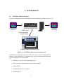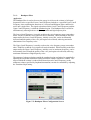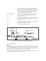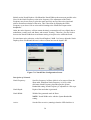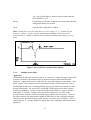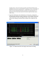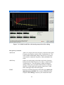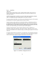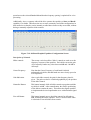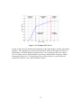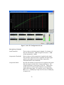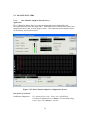
1
CARDINAL
AccelCore 24/192
AccelCore LE
User’s Manual
AudioLab Version 2.3.0
CARDINAL
AccelCore 24/192
AccelCore LE
User’s Manual
AudioLab Version 2.3.0
September 2011
Version 2.3.0
4018 Patriot Drive
One Park Center
Suite 300
Durham, NC 27703
Phone: 919 572 6767
Fax:
919 572 6786
[email protected]
www.dacaudio.com
Copyright © 2005-2011 by Digital Audio Corporation.
All rights reserved.
Table of Contents
1: WHAT’S NEW (OR DIFFERENT)? ............................................................................ ix
2: SYSTEM BASICS.......................................................................................................... 1
2.1: System Configuration .............................................................................................. 1
2.2: AccelCore 24/192 Capabilities ................................................................................ 2
2.3: AccelCore 24/192 Front Panel ................................................................................. 2
2.3.1: HEADPHONES Section ............................................................................... 3
2.3.2: AUXILIARY INPUT.................................................................................... 3
2.3.3: SAMPLE RATE Indicator ............................................................................ 3
2.3.4: DSP UTILIZATION Indicator ..................................................................... 4
2.3.5: Status LEDs .................................................................................................. 4
2.3.6: POWER Switch ............................................................................................ 4
2.4: ACCELCORE 24/192 REAR Panel ........................................................................ 5
2.4.1: AC POWER Input......................................................................................... 5
2.4.2: CONTROL INTERFACE............................................................................. 5
2.4.3: EXPANSION INTERCONNECT ................................................................ 6
2.4.4: WORD SYNC ............................................................................................... 6
2.4.5: BALANCED ANALOG INPUT PAIRS ...................................................... 6
2.4.6: BALANCED ANALOG OUTPUT PAIRS .................................................. 6
2.4.7: MONITOR OUTPUT ................................................................................... 7
2.4.8: AES/EBU and S/PDIF Digital Inputs and Outputs ...................................... 7
2.4.9: TOSLINK Digital Inputs and Outputs .......................................................... 7
2.4.10:
ADAT Digital Inputs and Outputs ............................................................ 7
2.5: AccelCore LE Capabilities ...................................................................................... 8
2.6: AccelCore LE Front Panel ....................................................................................... 9
2.6.1: HEADPHONES Section ............................................................................... 9
2.6.2: AUXILIARY INPUT.................................................................................... 9
2.6.3: Status LEDs ................................................................................................ 10
2.6.4: POWER Switch .......................................................................................... 10
2.7: ACCELCORE LE REAR Panel ............................................................................ 10
2.7.1: DC POWER Input....................................................................................... 10
2.7.2: CONTROL INTERFACE........................................................................... 11
2.7.3: ANALOG INPUTS..................................................................................... 11
2.7.4: ANALOG OUTPUTS................................................................................. 11
2.7.5: MONITOR OUTPUT ................................................................................. 11
2.7.6: TOSLINK 1 and S/PDIF Digital Inputs and Outputs ................................. 11
2.7.7: ADAT Digital Inputs and Outputs .............................................................. 12
2.7.8: ACCELCORE LE Mounting Options ........................................................ 12
3: Overview of Terms and Concepts ................................................................................ 15
4: Workspace Overview.................................................................................................... 17
4.1: ToolBox ................................................................................................................. 17
4.2: Monitor Display (ACCELCORE 24/192 ONLY) ................................................. 19
4.3: System Status ......................................................................................................... 19
4.4: Workspace ............................................................................................................. 20
5: PROJECTS ................................................................................................................... 21
v
5.1: Creating Projects .................................................................................................... 21
5.2: PRINTING/EXPORTING REPORTS .................................................................. 21
5.2.1: Print Report ................................................................................................. 21
5.2.2: Print Preview ............................................................................................... 22
5.2.3: Export Report .............................................................................................. 22
5.2.4: Report Customization ................................................................................. 23
5.3: PROJECT PROPERTIES ...................................................................................... 23
5.3.1: Project Information ..................................................................................... 23
5.3.2: Company/Agency Information ................................................................... 24
5.3.3: Author/Examiner Information .................................................................... 25
5.3.4: Report Logo ................................................................................................ 26
5.3.5: Print Settings ............................................................................................... 27
6: FILTER CHAINS ......................................................................................................... 29
6.1: FILTER CHAIN Management .............................................................................. 29
6.1.1: Adding a new filter chain ............................................................................ 29
6.1.2: Removing a filter chain ............................................................................... 29
6.2: Route Management ................................................................................................ 30
6.3: Selecting Routes .................................................................................................... 32
6.4: Changing Routes .................................................................................................... 33
6.5: ASIO AUDIO STREAMING ................................................................................ 33
6.5.1: Configuring Adobe Audition 2.0 ................................................................ 34
6.5.2: Playing WAV files ...................................................................................... 34
6.5.3: Recording WAV files ................................................................................. 34
6.5.4: Playing and Recording WAV files ............................................................. 35
6.5.5: ASIO Performance Optimizations .............................................................. 35
6.6: Filter Management ................................................................................................. 36
6.6.1: Adding Filters ............................................................................................. 36
6.6.2: Moving Filters ............................................................................................. 38
6.6.3: Deleting Filters............................................................................................ 38
6.7: Selecting Visualizations ......................................................................................... 38
6.7.1: Spectrum Analyzer Visualization ............................................................... 39
6.8: Selecting Monitors ................................................................................................. 40
7: Filters ............................................................................................................................ 41
7.1: Bandlimiting Filters ............................................................................................... 41
7.1.1: Lowpass Filter ............................................................................................. 41
7.1.2: Highpass Filter ............................................................................................ 43
7.1.3: Bandpass Filter............................................................................................ 45
7.1.4: Bandstop Filter ............................................................................................ 47
7.1.5: Notch Filter ................................................................................................. 49
7.1.6: Multiple Notch Filter .................................................................................. 51
7.1.7: Slot Filter .................................................................................................... 56
7.1.8: Multiple Slot Filter ...................................................................................... 57
7.1.9: Comb Filter ................................................................................................. 61
7.2: Equalizers............................................................................................................... 64
7.2.1: 20-Band Graphic Equalizer......................................................................... 64
7.2.2: High-Resolution Graphic Equalizer ............................................................ 66
vi
7.2.3: Parametric Equalizer ................................................................................... 68
7.3: Level Controls........................................................................................................ 70
7.3.1: Digitally-Controlled AGC .......................................................................... 70
7.3.2: Digitally-Controlled Limiter/Compressor/Expander .................................. 72
7.4: Adaptive Filters...................................................................................................... 76
7.4.1: One Channel Adaptive (Deconvolver)........................................................ 76
7.4.2: Reference Canceller .................................................................................... 78
7.5: Broadband Filters ................................................................................................... 81
7.5.1: NoiseEQ ...................................................................................................... 81
7.5.2: Noise Reducer ............................................................................................. 84
7.5.3: Adaptive Spectral Inverse Filter (ASIF) ..................................................... 85
7.5.4: Spectral Inverse Filter ................................................................................. 93
7.6: DIRECTX PLUGINS ............................................................................................ 99
7.6.1: Acon Digital Media StudioDenoiser ........................................................... 99
7.6.2: Acon Digital Media StudioDeclicker........................................................ 101
7.6.3: Acon Digital Media StudioDeclipper ....................................................... 102
8: Visualizations ............................................................................................................. 104
8.1: Spectrum Analyzer .............................................................................................. 104
8.2: Coefficient Display .............................................................................................. 105
9: SPECIFICATIONS (CARDINAL FORENSIC EXAMINER PACKAGE WITH
ACCELCORE 24/192 HARDWARE) ........................................................................... 108
10: SPECIFICATIONS (CARDINAL TECH AGENT PACKAGE WITH ACCELCORE
LE HARDWARE) .......................................................................................................... 113
vii
viii
1: WHAT’S NEW (OR DIFFERENT)?
The latest version 2.3.0 AudioLab software has been enhanced to now support 64-bit
operating systems. This includes 64-bit versions of Windows XP, Vista and Windows 7.
However, because of the way this new driver operates, only sample rates above 32kHz are
now supported.
ix
2: SYSTEM BASICS
2.1:
SYSTEM CONFIGURATION
The basic configuration of the CARDINAL system is illustrated as follows (Figure 2-1):
AccelCore (24/192 or LE)
Original Noisy
Recording
IEEE-1394a
(Control and Multichannel Audio)
Windows-Based AudioLab Software
Figure 2-1: CARDINAL Basic System Configuration
CARDINAL can currently be operated on 32-bit or 64-bit versions of Windows® XP,
Windows Vista, and Windows 7 computers, only. For best performance the following
system configuration is recommended:
•
Windows® 7 32-bit or 64-bit operating system
•
Intel Core2 Duo CPU processor (at least 2GHz or higher)
•
2 GB of RAM
•
120GB hard disk drive (or larger)
•
CD-ROM Drive
1
Enhanced
Recording
•
Dual 22” 1680x1050 flat-panel displays
•
Two-button optical mouse
•
IEEE-1394a “Firewire” interface (adaptor cable required for IEEE-1394b jacks)
•
Color laser or inkjet printer
Performance will improve with higher speed CPUs and/or increased memory.
2.2:
ACCELCORE 24/192 CAPABILITIES
The CARDINAL AccelCore 24/192 unit is a high-performance, self-contained digital signal
processor and contains 11 high-performance DSP microprocessors, which are allocated as
follows:
•
8 Analog Devices TigerSHARC floating-point audio processors, which implement
all audio processing functions in real-time via high-performance DSP firmware
•
One additional TigerSHARC floating-point audio processor and custom FPGA
interface for digital signal conditioning
•
One Wavefront Semiconductor DICE II application-specific IC and ARM core,
which provides the Firewire audio and control interface and controls all digital audio
routing functions
•
One Texas Instruments TMS320VC5410A signal processor, which performs the
audio monitoring function and operates the high-precision front panel bargraphs
Analog-to-digital and digital-to-analog conversion is performed by stereo, 24-bit, sigmadelta converters which perform 128x oversampling.
The base processing sample rate is currently adjustable from 16 kHz (7.5 kHz bandwidth) to
96 kHz (44 kHz bandwidth), regardless of the input sample rate when the digital input is
used (sample rates from 25-200 kHz are supported via asynchronous conversion). All
processing is implemented using floating-point arithmetic for maximum computational
precision and reduced quantization noise as compared with fixed-point systems.
2.3:
ACCELCORE 24/192 FRONT PANEL
The front panel of the CARDINAL AccelCore 24/192 appears as follows:
2
Figure 2-2: CARDINAL AccelCore 24/192 Front Panel
The front panel controls are arranged into five logical groups: HEADPHONES and
MONITOR controls, convenience AUXILIARY INPUT jacks, SAMPLE RATE, and DSP
UTILIZATION indicators, status indicator LEDs, and POWER switch.
2.3.1:
HEADPHONES Section
The HEADPHONES allow the user to listen to the monitor signal (mono or stereo pair) as
selected by the AudioLab software, control the listening level via a dedicated volume knob,
and view the audio level via dual high-precision 53-segment bargraphs. Dual 1/4" PHONES
jacks are provided, allowing for two listeners in the forensic processing application
(examiner and agent/client, for example). Additionally, the same monitor signal pair is
available on the rear-panel MONITOR outputs, which can be directly connected to powered
monitor speakers, e.g. “near-field” monitors as may be found in studios. Because such
monitors are often not located within easy reach, an additional dedicated volume knob and
speaker on/off switch is provided. Also, dedicated 53-segment bargraphs are provided. Note
that switching the monitored signal(s) does not alter the signal flow to the other analog and
digital output connectors, which are normally connected to recording equipment to capture
the enhanced audio output from the CARDINAL. This allows real-time comparison of
before/after audio to be made without affecting the copying operation in progress.
2.3.2:
AUXILIARY INPUT
The AUXILIARY INPUT section allows quick connection of analog or digital audio signals
from unusual sources, e.g. radio receivers, Sony NT-2 recorders, solid-state pocket
recorders, etc. To use these, simply connect the device to the appropriate jack(s) and select
the source within the AudioLab software; for devices connected to the DIGITAL input, the
AccelCore will automatically synchronize to the device sample rate, as long as it is within
the range of 25-200 kHz and conforms to the IEC 60958-3 standard for optical digital audio
interconnect.
2.3.3:
SAMPLE RATE Indicator
The SAMPLE RATE indicator gives the user a quick indication of the sample rate at which
the processors are operating. Note that with the exception of the ADAT® interfaces, this is
3
completely independent of the sample rates at which the digital inputs and outputs are
operating, due to the AccelCore’s asynchronous sample rate conversion capability (ADAT
must always be operated at the same sample rate as the processing, as there is no sample rate
conversion on this interface). In the current version of the AudioLab software, only sample
rates between 32 and 48 kHz are supported. If performing audio streaming via ASIO, the
sample rate must be at least 32 kHz due to the AccelCore hardware.
2.3.4:
DSP UTILIZATION Indicator
The DSP UTILIZATION gives the user a quick indication of the percentage amount of DSP
resources currently being utilized. For example, “10” would indicate that 10% of resources
are being used; obviously, the maximum indication would be “100”, at which point all the
DSP capability has been fully consumed. Future “expansion” hardware that makes use of
the rear-panel expansion connectors will allow additional DSP resource to be brought online
if high utilization is routinely encountered.
2.3.5:
Status LEDs
The status LEDs indicate various states of operation, including LINK and ACTIVITY status
of the Firewire interface. When the IEEE-1394a cable has been properly connected between
the AccelCore and the PC (or to another “daisy-chained” device), the LINK LED should be
illuminated. Whenever there is actual communication taking place between the AudioLab
software and the AccelCore, the AUDIO LAB LED should be illuminated, with the
ACTIVITY LED occasionally flashing whenever controls are being adjusted, etc. The ASIO
LED may also illuminate whenever the audio streaming functionality is being utilized. The
POWER led indicates when power is supplied to the unit; all other front panel status LEDs
are reserved for future software updates.
2.3.6:
POWER Switch
The POWER switch must be switched to the ON position for normal operation of the unit;
as the AccelCore consumes approximately 50W of power under normal operation, for
energy conservation it is recommended to switch the power OFF when the unit is not in use.
4
2.4:
ACCELCORE 24/192 REAR PANEL
The rear panel of the AccelCore 24/192 appears as follows:
Figure 2-3: CARDINAL AccelCore 24/192 Rear Panel
2.4.1:
AC POWER Input
AC power is provided to the unit through the IEC320 inlet jack using the appropriate mains
cord for the particular country. The internal power supply is of the “universal” variety,
capable of automatically accommodating mains voltages in the range of 85-264VAC and
mains bus frequencies between 47 and 63 Hz. A 2 Ampere fast-blow fuse is provided for
safety, but should never need to be replaced with normal product operation. The front-panel
POWER switch must be switched to the ON position in order for the unit to operate.
2.4.2:
CONTROL INTERFACE
Dual IEEE-1394a 6-pin connectors are provided to connect the AccelCore to a computer
using the supplied cable. Either port can be used to connect the cable to the PC; the second
jack can be used to “daisy-chain” a cable connection to any other Firewire device (e.g. a
Digi002 unit, as described earlier), although it is generally recommended that the AccelCore
be given a dedicated connection with no other equipment on the bus. When the AudioLab
software (which includes device drivers) is properly installed on the PC, and is run, the
AccelCore will automatically begin communicating with the software and normal operation
will begin. When a proper cable connection is made, the LINK LEDs (the one on the rear
panel provides an identical indication to the one on the front panel) will illuminate solidly;
as indicated in the front panel section, the front-panel AUDIO LAB and ACTIVITY LEDs
will illuminate whenever the AudioLab software is running.
5
2.4.3:
EXPANSION INTERCONNECT
“HDMI”-style connectors, which support high-speed digital communication via LVDSsignaling, are provided in order to allow for a future DSP upgrade capability via add-on
AccelCore Expansion boxes.
2.4.4:
WORD SYNC
A TTL-compatible transformer-coupled BNC jack is provided to allow other digital audio
equipment to be synchronized to the AccelCore sample clock via standard 75-ohm BNC
cabling. For normal operation, however, this connection is not needed, due to the
AccelCore’s asynchronous sample rate conversion capability; all that is needed is to set the
digital output sample rate and format to one that is compatible with the equipment.
2.4.5:
BALANCED ANALOG INPUT PAIRS
Eight channels of analog input are provided via ¼” “TRS” style balanced interconnects.
Normally stereo analog equipment is connected to the AccelCore in pairs, e.g. INPUT PAIR
1 L and R; in this manner, up to four stereo analog decks or 8 monaural decks can be
connected directly to the AccelCore. Wiring of the input jacks is as follows: TIP = “+”,
RING = “-”, and SLEEVE = AC GROUND. To avoid ground looping issues, it is
recommended that balanced connection always be utilized; however, in cases where singleended equipment (e.g. equipment with analog RCA jack outputs) must be connected, an
RCA-1/4” adaptor plug of the type pictured below can be utilized.
Figure 2-4: RCA-1/4” Adaptor Plugs
For connection to equipment with standard XLR balanced interconnects, please use XLRTRS adaptor cables which are wired as follows: XLRp.2 to TIP, XLRp.3 to RING, and
XLRp.1 to SLEEVE. This is a standard cable normally available from most any audio
supply house. For equipment with TRS balanced interconnects, a TRS-TRS cable wired TIP
to TIP, RING to RING, and SLEEVE to SLEEVE should be used; again, this is a standard
cable available from most any audio supply house. Should you have difficulty obtaining
proper interconnect cabling, please contact DAC and we will be happy to supply it for you.
2.4.6:
BALANCED ANALOG OUTPUT PAIRS
As with the BALANCED INPUT PAIRS, eight channels of analog output are provided via
¼” “TRS” style balanced interconnects. Wiring of the input jacks is as follows: TIP = “+”,
RING = “-”, and SLEEVE = CHASSIS GROUND. Again, to avoid ground looping issues,
6
it is recommended that balanced connection always be utilized; as with the analog inputs, if
equipment that uses RCA jacks must be connected to the AccelCore, the RCA-1/4” adaptor
plugs previously mentioned can be utilized.
2.4.7:
MONITOR OUTPUT
The MONITOR OUTPUT jacks are identical to the BALANCED ANALOG OUTPUT
PAIRS, except that their volume can be controlled by the MONITOR volume knob on the
front panel and they are affected by the SPEAKERS ON/OFF switch. Any signal(s) within
the processing chain can be selected for output to the MONITOR OUTPUT; the same signal
is also applied to the front-panel HEADPHONES outputs.
2.4.8:
AES/EBU and S/PDIF Digital Inputs and Outputs
The AES/EBU and S/PDIF jacks provide easy interconnect with most high-end digital
recording equipment, e.g. CD recorders, DAT recorders, MiniDisc recorders, etc. In the case
of the AES/EBU jacks, XLR-style cabling must be utilized; for the S/PDIF jacks, normal
RCA cabling can be used. The AES/EBU connections are preferred whenever connecting to
devices that are more than 10 feet away from the AccelCore processor. Two important
points to remember with these particular connections: first, as inputs only one can be utilized
by the AccelCore at a time. Secondly, as outputs they are “mirrored”, in that both provide
the same channels of digital output data; whatever audio is on one of them will be on the
other.
2.4.9:
TOSLINK Digital Inputs and Outputs
The optical “TOSLINK” jacks provide easy interconnect with most high-end digital
recording equipment, e.g. CD recorders, DAT recorders, MiniDisc recorders, etc. When
these interconnects are used, fiber-optic cabling with compatible “Toshiba”-style plugs must
be utilized. In the case where the recording equipment has AES/EBU or S/PDIF non-optical
connections, an adaptor box (e.g. the M-Audio Model CO2 product) can be utilized to
convert the electrical signal into a compatible optical signal. Unlike the AES/EBU and
S/PDIF jacks, all the TOSLINK jacks are independent; this means the AudioLab software
can route signals to them independently for separate recording.
2.4.10:
ADAT Digital Inputs and Outputs
The optical ADAT “Light Pipe” digital interconnects provide an easy way to integrate the
AccelCore with other professional-grade multichannel sound devices, e.g. the Digidesign
Digi002 unit as described earlier. The ADAT input and output support eight audio channels
simultaneously and always operate at the system sample rate as indicated on the front panel
display.
7
2.5:
ACCELCORE LE CAPABILITIES
The CARDINAL AccelCore LE unit is a high-performance, self-contained digital signal
processor and contains 5 high-performance DSP microprocessors, which are allocated as
follows:
•
4 Analog Devices TigerSHARC floating-point audio processors, which implement
all audio processing functions in real-time via high-performance DSP firmware
•
One additional TigerSHARC floating-point audio processor and custom FPGA
interface for digital signal conditioning
•
One Wavefront Semiconductor DICE II application-specific IC and ARM core,
which provides the Firewire audio and control interface and controls all digital audio
routing functions
Analog-to-digital and digital-to-analog conversion is performed by stereo, 24-bit, sigmadelta converters which perform 128x oversampling.
The base processing sample rate is currently adjustable from 32 kHz to 48 kHz, regardless
of the input sample rate when the digital input is used (sample rates from 25-200 kHz are
supported via asynchronous conversion). All processing is implemented using floating-point
arithmetic for maximum computational precision and reduced quantization noise as
compared with fixed-point systems.
8
2.6:
ACCELCORE LE FRONT PANEL
The front panel of the CARDINAL AccelCore LE appears as follows:
Figure 2-5: CARDINAL AccelCore LE Front Panel
The front panel controls are arranged into four logical groups: HEADPHONES and
VOLUME control, analog AUXILIARY INPUT jack, status indicator LEDs, and POWER
switch.
2.6.1:
HEADPHONES Section
The HEADPHONES allow the user to listen to the monitor signal (mono or stereo pair) as
selected by the AudioLab software and control the listening level via a VOLUME knob.
Dual 3.5mm stereo headphone jacks are provided, allowing for two listeners in the forensic
processing application (examiner and agent/client, for example). Additionally, the same
monitor signal pair is available on the rear-panel digital MONITOR OUTPUT, which can
be directly connected to powered monitor speakers that have an optical digital input (such as
the Edirol MA-15D). Note that switching the monitored signal(s) and changing the volume
level does not alter the signal flow to the rear-panel analog and digital output connectors,
which are normally connected to recording equipment to capture the enhanced audio output
from the CARDINAL. This allows real-time comparison of before/after audio to be made
without affecting the copying operation in progress.
2.6.2:
AUXILIARY INPUT
The AUXILIARY INPUT section allows quick connection of analog audio signals from
unusual sources, e.g. radio receivers, solid-state pocket recorders, etc. To use these, simply
connect the device and select the source within the AudioLab software.
9
2.6.3:
Status LEDs
The status LEDs indicate various states of operation, including LINK and ACTIVITY status
of the Firewire interface. When the IEEE-1394a cable has been properly connected between
the AccelCore and the PC (or to another “daisy-chained” device), the LINK LED should be
illuminated. Whenever there is actual communication taking place between the AudioLab
software and the AccelCore, the AUDIO LAB LED should be illuminated, with the
ACTIVITY LED occasionally flashing whenever controls are being adjusted, etc. The ASIO
LED may also illuminate whenever the audio streaming functionality is being utilized.
2.6.4:
POWER Switch
The POWER switch must be switched to the ON position (with the BLUE power LED
illuminated) for normal operation of the unit; as the AccelCore consumes approximately
50W of power under normal operation, for energy conservation it is recommended to switch
the power OFF when the unit is not in use.
2.7:
ACCELCORE LE REAR PANEL
The rear panel of the AccelCore LE appears as follows:
Figure 2-6: CARDINAL AccelCore LE Rear Panel
2.7.1:
DC POWER Input
DC power (nominally 12VDC) is provided to the unit via an external “universal” AC
adaptor that includes the appropriate mains cord for the particular country. Mains voltages in
the range of 85-264VAC and mains bus frequencies between 47 and 63 Hz are all
accommodated automatically (no switching or rewiring is required). An internal resettable
fuse is provided for safety, and never requires replacement. The front-panel POWER switch
must be switched to the ON position (with the blue LED illuminated) in order for the unit to
operate.
10
2.7.2:
CONTROL INTERFACE
A single IEEE-1394a 6-pin connector is provided to connect the AccelCore to a computer
using the supplied cable. It is highly recommended that the AccelCore be given a dedicated
connection to the computer with no other equipment on the bus. When the AudioLab
software (which includes device drivers) is properly installed on the PC, and is run, the
AccelCore will automatically begin communicating with the software and normal operation
will begin. When a proper cable connection is made, the LINK LEDs (the one on the rear
panel provides an identical indication to the one on the front panel) will illuminate solidly;
as indicated in the front panel section, the front-panel AUDIO LAB and ACTIVITY LEDs
will illuminate whenever the AudioLab software is running.
2.7.3:
ANALOG INPUTS
Two channels of analog input are provided via standard “line-level” RCA interconnects.
These connections are ground-isolated for improved noise immunity and minimal “groundlooping” issues.
2.7.4:
ANALOG OUTPUTS
Two channels of analog output are provided via standard “line-level” RCA interconnects.
These connections are single-ended, or “unbalanced”; therefore, cable lengths to connected
equipment should be kept as short as possible to minimize any potential noise and/or
ground-looping issues.
2.7.5:
MONITOR OUTPUT
The digital MONITOR OUTPUT jack provides a means of connecting external amplified
loudspeakers that support the connection of a “TOSLINK”, or optical digital source via
fiberoptic cable. An example of such speakers is the Edirol MA-15D, typically supplied by
DAC as a standard component of a turnkey audio workstation using the CARDINAL. Any
signal(s) within the processing chain can be selected for output to the MONITOR OUTPUT;
the same signal is also applied to the front-panel HEADPHONES outputs.
2.7.6:
TOSLINK 1 and S/PDIF Digital Inputs and Outputs
The TOSLINK 1 and S/PDIF jacks provide easy interconnect with most high-end digital
recording equipment, e.g. CD recorders, DAT recorders, MiniDisc recorders, etc. For the
TOSLINK connection, optical cabling is required; for the S/PDIF connection, normal RCA
cabling can be used. The optical TOSLINK connections are preferred whenever connecting
to devices that are more than 10 feet away from the AccelCore processor. Two important
points to remember with these particular connections: first, as inputs only one can be utilized
by the AccelCore at a time. Secondly, as outputs they are “mirrored”, in that both provide
the same channels of digital output data; whatever audio is on one of them will be on the
other.
11
2.7.7:
ADAT Digital Inputs and Outputs
The rear-panel optical connectors can be optionally configured by the AudioLab software to
operate in either the TOSLINK or ADAT digital mode. In the ADAT mode, the optical
digital interconnects provide an easy way to integrate the AccelCore with other professionalgrade multichannel sound devices, e.g. the Digidesign Digi002. The ADAT input and output
support eight audio channels simultaneously and always operate at the system sample rate
(no automatic sample rate conversion is provided in the ADAT mode).
2.7.8:
ACCELCORE LE Mounting Options
The AccelCore LE comes with all required the hardware to support three different
mounting / usage options as pictured below:
Figure 2-5: CARDINAL AccelCore LE – Horizontal Desktop Usage
12
Figure 2-6: CARDINAL AccelCore LE – Vertical Desktop Usage Using Special Base
Plate (Included)
13
Figure 2-7: CARDINAL AccelCore LE – Rack Mounting Using Special Rack
Extender and Rack Ears (Included)
14
3: OVERVIEW OF TERMS AND CONCEPTS
AudioLab uses the concepts of Filter Chains, Routes and Filters to describe the flow of
audio through the system.
A Filter is a process that manipulates the audio passing through it. This term is used
generally to describe traditional filters like a Lowpass Filter, as well as Equalizers and
Level Controls.
A Route establishes an association between a given input and a given output. Any audio
input can be routed through the system with the result given on any output. For instance,
the audio can be taken in the rear panel Analog 1 jacks, routed through a series of filters,
and the output be given on the ADAT output jacks. The association of the Analog 1
input jacks and the ADAT output jacks is called a Route.
A Filter Chain is simply a container for Routes and Filters. A Filter Chain must have at
least one Route, but at present, no more than two (this allows for mono or stereo
channels). A Filter Chain can have zero or more Filters – the maximum number of
filters will vary depending on what types of filters are being used.
Figure 3-1 describes the relationship of all three components. Here, a single route is
defined (Front Analog (L) is routed to Analog 4 (L)) along with two filters.
Filter Chain
Front
Analog (L)
Flow of Audio
Filter 1
Lowpass
Filter 2
20-Band
EQ
Analog 4
(L)
Figure 3-1: Filter Chain with One Route and Two Filters
Figure 3-2 adds another route to the chain making it a stereo filter chain.
15
Filter Chain
Front
Analog (L)
Flow of Audio
Filter 1
Lowpass
Filter 2
20-Band
EQ
Front
Analog (R)
Analog 4
(L)
Analog 4
(R)
Figure 3-2: Filter Chain with Two Routes and Two Filters
This scenario is referred to as a stereo-linked filter chain. Both routes of audio are
logically passing through the same set of filters (although physically, they may be passing
through separate but identical filters, depending on the filter type). If you wanted to have
completely independent filtering for each route, then you would separate them into two
mono filter chains.
16
4: WORKSPACE OVERVIEW
The AudioLab user interface (shown in Figure 4-1) consists primarily of a workspace
into which users can add filter chains. Once a filter chain is present, users can drag-anddrop filters and presets into the chain. A filter chain is the primary unit of work in
AudioLab.
Figure 4-1: AudioLab Workspace
4.1: TOOLBOX
The AudioLab Toolbox area contains filters and presets that users can drag and drop into
filter chains. Filters are categorized into tool ‘drawers’. Clicking on a drawer’s title will
open that drawer and expose a new set of filters.
17
Figure 4-2: Filter Toolbox
There are 7 groups of filters available to users:
•
•
Bandlimiting Filters are those filters that typically attenuate a portion of the
signal’s frequency spectrum. Filters include:
o Lowpass
o Highpass
o Bandpass
o Bandstop
o Notch
o Multi-Notch
o Slot
o Multi-Slot
o Comb
Equalizers provide shaping of a signal’s frequency spectrum and are typically
used after all other processing is complete. Equalizers include:
18
•
•
•
•
•
o 20-Band Graphic
o Hi-Resolution Graphic
o Parametric EQ
Level Controls affect the level of the signal. These include:
o Automatic Gain Control (AGC)
o Limiter/Compressor/Expander (LCE)
Adaptive Filters will adapt their solutions in response to changes in the audio.
Filters include:
o One-Channel Adaptive (also known as a Deconvolver)
o Reference Canceller
Broadband Filters attack noise that is spread out over the signal’s entire
spectrum. Filters included:
o NoiseEQ
o Noise Reducer
o Adaptive Spectral Inverse Filter (ASIF)
o Spectral Inverse Filter (SIF)
Presets are those filters whose properties have been saved to a disk file (.PRE).
Since a preset is created by saving all filters in a given filter chain, a single preset
will contain 1 or more filters.
DirectX Plug Ins Special COM/ActiveX filters created for Microsoft’s
DirectShow platform (DirectX). These filters utilize the ASIO capabilities of the
Cardinal AccelCore hardware.
4.2: MONITOR DISPLAY (ACCELCORE 24/192 ONLY)
When the AccelCore 24/192 hardware is utilized, the monitoring display shows the user
the current levels of the headphone and monitor outputs. These bargraphs mimic those
on the front panel of the AccelCore hardware.
Figure 4-3: Monitor Controls
4.3: SYSTEM STATUS
The AccelCore hardware provides sample rates ranging from 16kHz to 96kHz. These are
selectable using the control found in the System Status area. The sample rate affects the
19
entire system and all filter chains. You cannot have different sample rates for different
filter chains simultaneously.
The AccelCore Resources bargraph indicates how much of the AccelCore hardware’s
capability is currently being utilized. As this number approaches 100%, some filters may
become unavailable to the user.
The ASIO Stream Utilization bargraph indicates how much of the I/O streaming is
currently being utilized. Up to 16 input and 16 output channels may be used
simultaneously. As this number approaches 100%, some DirectX/VST plugins may
become unavailable to the user.
Figure 4-4: System Status Area
4.4: WORKSPACE
The large open area in the user interface is referred to as the workspace. This space is
where filter chains are shown with their corresponding routes and filters. Each filter
chain is given its own window which can be minimized, maximized, moved, resized and
closed – all within the workspace area.
20
5: PROJECTS
Projects are created, modified, loaded, and saved within AudioLab. Each time AudioLab
starts, a copy of the last used project are automatically loaded into memory.
5.1: CREATING PROJECTS
To create a new AudioLab project, choose the New item from the File Menu (Figure
5-1). The project information tab of the Project Properties dialog will be displayed.
Although the information is optional, it is advised to at least enter a case ID since this
information is displayed in the AudioLab title bar as a page header on all generated
reports.
Once the project is created, an empty workspace is displayed and one or more filter
chains may be added. To save the project, choose the Save or Save As item from the File
Menu. To load an existing project, choose the Open item and browse to a previously
saved project.
Figure 5-1: File Menu
5.2: PRINTING/EXPORTING REPORTS
5.2.1:
Print Report
To print a report, choose the Print item from the File Menu and select a printer from the
displayed print dialog. Various print device options may be set in the standard Windows
print dialog.
21
5.2.2:
Print Preview
To preview a report without printing the report, choose the Print Preview item from the
File Menu. The AudioLab report will be displayed in a preview window exactly as it will
be printed. The preview image may be scaled and resized and the report may be printed
from the preview dialog if desired.
5.2.3:
Export Report
An AudioLab report may be exported to either an Adobe PDF file or a web page (HTML)
file. To export a report, choose the Export Report item from the File Menu. The report
export dialog will be displayed (Figure 5-2) and the report filename will be entered.
The preferred format is the PDF format since all images/graphics are contained within the
file. No additional software is required in order to generate a PDF report. In order to
view/read a PDF report, an Adobe PDF reader needs to be installed on the system. This is
a free software package from Adobe and has been included in the AudioLab installation
CD for your convenience.
The web page (HTML) format will save images & graphics to separate files that are
“linked” into the HTML document. The images are stored in a subdirectory where the
main HTML file is saved. The subdirectory is named using the HTML filename specified
when exporting the report.
22
Figure 5-2: Export Report Dialog
5.2.4:
Report Customization
Each AudioLab report may be somewhat customized for specific users/cases. The global
information (company, author, etc) as well as the displayed logo and font may be
changed prior to generating each report. Please review the Project Properties section
below for more information.
5.3: PROJECT PROPERTIES
The project properties dialog is displayed when a new project is created or the Project
Properties item is selected from the File menu.
5.3.1:
Project Information
The Project tab (Figure 5-3) contains information specific to the current project. All
information is stored with the project file.
Since the Case ID is displayed at the top of the screen and on all report pages, it is
recommended this field contain some valid information.
23
Figure 5-3: Project Information Tab
5.3.2:
Company/Agency Information
The Company tab (Figure 5-4) contains information specific to the company and/or
agency performing the audio analysis. This information is displayed on all reports and is
saved to the current project file. The company information is displayed on all generated
reports and the information is retained between different projects.
24
Figure 5-4: Company/Agency Information Tab
5.3.3:
Author/Examiner Information
The Author tab (Figure 5-5) contains information specific to the author and/or examiner
performing the audio analysis. This information is displayed on all reports and is saved to
the current project file. The author information is displayed on all generated reports and
the information is retained between different projects. The author’s initials are displayed
on all report page headers after the initial page.
25
Figure 5-5: Author/Examiner Information Tab
5.3.4:
Report Logo
The Logo tab (Figure 5-6) allows the user to specify what logo will appear on all
generated reports. The resolution of each logo is dependent on the print resolution.
The small company logo (default) is a logo displayed in the top-left corner of all reports.
The textual company information is displayed to the right of this logo. This logo should
conform to a 2-to-1 aspect ratio.
The wide company logo is displayed at the top of all reports and replaces the small logo
and the textual information. This option should be used if the small logo plus textual
company information is not adequate for generated reports. This logo should conform to
a 7-to-1 aspect ratio.
26
Figure 5-6: Logo Information Tab
5.3.5:
Print Settings
The Print Settings tab (Figure 5-7) allows the user to specify the paper size, orientation,
print margins, and font for all generated reports.
27
Figure 5-7: Print Settings Tab
28
6: FILTER CHAINS
Filter Chains are the unit of work in AudioLab. Nothing can really be done with the
system until a filter chain is defined with at least one route.
6.1: FILTER CHAIN MANAGEMENT
Filter Chain Management functions can be found in the Filter Chain menu. Users can
add new filter chains, remove the current filter chain (along with all its filters and routes)
and remove all filter chains.
Figure 6-1: Filter Chain Menu
6.1.1:
Adding a new filter chain
To add a new filter chain, click on the Filter Chain menu and then select Add Filter
Chain. Alternatively, you can use the keyboard shortcut of Ctrl+A. You will be
immediately prompted to select at least one route. Both an input and output source must
be selected (the Select Routes dialog will be covered in more depth later).
Once a route is selected, the new channel will appear in the workspace. Users can now
add filters to the chain to affect the audio flowing through the route(s).
Figure 6-2: Filter Chain Window
6.1.2:
Removing a filter chain
There are several ways to remove a filter chain. All techniques are equal in their effect of
closing the chain and removing all the filters and routes associated with that chain.
29
Perhaps the quickest and easiest way to remove a filter chain is to simply close the chain
window itself by clicking on the red “X” button in the top-right of the window. A chain
can also be removed by clicking on the Filter Chain menu and selecting Remove Current
Filter Chain. The current filter chain is defined as whichever chain window currently has
the focus in the workspace.
Figure 6-3: Remove Filter Chain Menu
6.2: ROUTE MANAGEMENT
Routes are always defined in the context of a filter chain. Routes for a particular filter
chain can be changed at any time. Each input and output channel of the Cardinal
AccelCore hardware may be assigned as an input/output route for any given filter chain.
Since it is usually more convenient to reference routes by attached device names (tape
deck, CDs, etc.) opposed to channel names (Analog 1 L, Front Panel R, etc), the
AudioLab software now allows the user to specify custom route names.
Although the custom route names are typically defined when hardware devices are
attached to the Cardinal, the route names may be changed at any time.
The User Defined Route Names dialog may be accessed by selecting the User Defined
Route Names option from the Tools menu. Additionally, the dialog may be accessed
when specifying filter chain routes via the Select Routes dialog.
30
Figure 6-4: User Defined Route Names Dialog (installed defaults)
Description of Controls
Add:
Adds a new route name row to the table. Each row must contain a
valid user defined Device Name, and I/O type, and at least a Left (L)
or Right (R) channel definition.
Remove:
Removes the currently selected route name row from the table.
Clear All:
Clears all user defined route names from the table.
Store:
Saves the current route names to a data file that may be imported at a
later time or on another machine running AudioLab.
Recall:
Imports a table of user defined route names from a specified data file.
I/O Column:
Click on this column to choose between Input, Output, or Both. A
device is considered an Input device if it is connected to a Cardinal
input channel and considered an Output device if connected to an
Output channel.
Selecting the Both type specifies that the Input and Output channels
are connected to the same device.
L & R Columns:
Specified either the left, right, or both (stereo) channels connected to
the device.
31
6.3: SELECTING ROUTES
When a filter chain is first added, the Select Routes dialog will appear first. This is
because a filter chain will not have audio running through it until at least one route is
defined for it.
Each route may have 1 input and 1 output channel (mono) or 2 input and 2 output
channels (stereo).
The Mono and Stereo tabs in the Select Route dialog provide a quick mechanism to
select single or double channel routes using similar devices. The Custom tab allows the
user to select up to 2 channels of input/output from different devices.
Figure 6-5: Select Mono Routes
Figure 6-6: Select Stereo Routes
32
Figure 6-7: Select Custom Routes
In order for the “OK” button to be enabled, users must make a valid selection for both the
Input and Output of Route 1. Any input can be routed to any output. Once users have
made a valid selection, then the “OK” button will be enabled as well as the selection
boxes for Route 2. If a user wants a stereo-linked filter chain, he may specify the signals
for Route 2 now. Clicking “OK” will then dismiss the dialog and show the filter chain
with the proper routes.
6.4: CHANGING ROUTES
Changing a route once it’s been defined and the filter chain is passing audio is not much
different than selecting the original routes. Users click on the “Routes” button in the
Input section of the filter chain window and the Select Routes dialog will appear with the
current selections. Users can then change the existing route(s) and click “OK”.
Changing routes will not result in filter settings being changed, lost or reset.
6.5: ASIO AUDIO STREAMING
AudioLab provides the capability to stream audio data to/from a 3rd party application
using Steinberg’s ASIO 2.0 interface. AudioLab allows up to 16 input and 16 output
streaming channels to be simultaneously processed within a given session. In addition,
DirectX plug-ins (Microsoft DirectShow) may be placed in a filter chain along with other
internal Cardinal filters.
Due to the design of the Cardinal AccelCore hardware, the sample rate must be set to at
least 32 kHz for audio streaming to work correctly.
Note: A minimum of a 2GHz CPU is required to perform audio streaming via ASIO.
33
The following steps illustrate how to use Adobe Audition 2.0 with the Cardinal AudioLab
software to play & record WAV files. Please note that any software that supports ASIO
2.0 can be used to stream audio channels to/from the Cardinal AccelCore.
6.5.1: Configuring Adobe Audition 2.0
1. Make sure the AudioLab software is installed and the Cardinal AccelCore
hardware is turned on.
2. Start Adobe Audition 2.0
3. Select Audio Hardware Setup from the Edit menu.
4. Select the Edit View tab
5. Make sure ASIO Dice is selected as the audio driver in the drop-down list.
6. Select the Multitrack View tab
7. Make sure ASIO Dice is selected as the audio driver in the drop-down list.
8. Click OK to save the changes
6.5.2: Playing WAV files
1.
2.
3.
4.
5.
6.
7.
Start Adobe Audition 2.0
Select Multitrack from the Adobe Audition toolbar
Select the Import… item from the File menu
Choose the audio file (WAV or other) to import
Drag and drop the imported file into an available track (i.e. Track 1)
Set the track input to None.
Leave the track out set to Master or choose a mono Cardinal ASIO Stream
channel (1..16). Master implies ASIO stream channel’s 1 & 2.
8. Start the AudioLab software and add a filter chain
9. Click the Route button to display the Route dialog
10. Set the input Route 1 to ASIO Stream 1 (or whatever ASIO channel was
specified in step 7)
11. Set the Route 1 output to the desired output channel
12. Repeat for Route 2 if creating a stereo route. This time specify ASIO Stream 2 for
the channel (to match the channel specified in Adobe Audition)
13. Click OK to save the route.
14. In Adobe Audition, click the Play button to start playing the audio file.
The streaming audio should now show up in the AudioLab software
6.5.3: Recording WAV files
1. Start the AudioLab software and add a filter chain
2. Click the Route button to display the Route dialog
3. Set the input route to the input source and set the output Route 1 to ASIO
Stream 1
4. Repeat for Route 2 if creating a stereo route. This time specify ASIO Stream 2 for
the channel (to match the channel specified in Adobe Audition)
5. Click OK to save the route
34
6. Start Adobe Audition 2.0
7. Select Multitrack from the Adobe Audition toolbar
8. Select a track and set the input to Stereo (if using Cardinal ASIO stream 1 & 2)
or Mono (and select Cardinal ASIO stream 1)
9. Click the red “Arm for Record” button in the track UI
10. Enter a session filename when prompted
11. Begin playing the AudioLab input source specified when creating the Filter Chain
Route
12. Click the Audition Record button (in the transport UI) to start recording the WAV
file
13. Click the Audition Stop button (in the transport UI) to stop recording
14. The WAV file will be saved to the location specified when naming the Audition
session.
6.5.4: Playing and Recording WAV files
It is possible to play a WAV file from Adobe Audition and send the output to the
Cardinal and record the processed audio back in Adobe Audition.
1. Setup Adobe Audition Track 1 to play an audio file to Cardinal ASIO stream 1
(and optionally Cardinal ASIO stream 2)
2. Setup a filter chain in the Cardinal AudioLab software with the input route using
ASIO stream 1 (and optionally ASIO stream 2 for stereo).
3. Set the AudioLab output route to ASIO stream 3 (and optionally ASIO stream 4
for stereo)
4. Setup Adobe Audition Track 2 to record from Cardinal ASIO stream 3 (and
optionally Cardinal ASIO stream 4 for stereo).
5. Click the “Arm for Record” in Audition Track 2 and enter a session filename if
prompted (i.e. session does not already exist)
6. Click the Audition Record button to start playback/recording
7. The resultant WAV file will be saved with the session
6.5.5: ASIO Performance Optimizations
In order to improve the performance of the ASIO streaming, the following
optimizations/settings should be considered. Please consult your system administrator
if necessary.
•
•
•
•
•
•
CPU speed should be 2GHz minimum
Increase system RAM to at least 1GB
Avoid running unneeded program at the same time as AudioLab or Adobe
Audition.
Turn off any software utilities that run in the background, such as Windows
Messenger, calendars, and disk maintenance programs.
Turn off nonessential USB devices while running AudioLab & Adobe Audition.
Disable network cards if possible
35
•
Stop any unnecessary Windows services and system startup items. Please be
careful when stopping Windows services. One approach is to use the MSCONFIG
utility and boot up the system in Diagnostic Startup mode. Then start adding only
the necessary Windows services.
6.6: FILTER MANAGEMENT
Once a filter chain and at least one route are defined, users can then begin adding filters
to the chain. AudioLab utilizes a drag-and-drop interface for adding and moving filters.
6.6.1:
Adding Filters
To add a new filter to a filter chain, users should drag the filter from the toolbox and drop
it into the filter chain window. Where it is dropped in the window will determine its
position in the chain of filters. There is a line in the window that highlights where the
user is about to drop the filter. If it is between two other filters, the filter will be inserted
between the two filters.
Figure 6-8: Insert a new filter – Step 1: Click and Drag
36
Figure 6-9: Insert a new filter – Step 2: Drag into filter chain
Figure 6-10: Insert a new filter – Step 3: Drop into filter chain
37
6.6.2:
Moving Filters
To move a filter from one position to another in the chain, users simply click anywhere
on the background of the desired filter and drag it into its new position.
6.6.3:
Deleting Filters
To delete a filter, click on the “X” button in the top-right corner of the filter box. If you
close the entire filter chain, then all the filters in the chain will also be deleted.
6.7: SELECTING VISUALIZATIONS
There are currently two kinds of visualizations available for the AudioLab system: a 512point spectrum analyzer and a coefficient display.
Users can view the spectrum of a signal at any point in the filtering process, including the
raw input and the final output, using the spectrum analyzer. Users cannot view the
spectrum of a signal that is not currently part of a filter chain. For instance, if Analog 1
(L) is selected as input and Analog 2 (L) is selected as output, the user cannot view
Analog 4 (L) even though a signal may be connected to the input jack.
The coefficient display is only available on certain filters for which it would be
meaningful; mainly the 1-Channel adaptive and Reference Canceller filters. The display
is shown on the filter’s configuration screen, which the user can access through the
Config button.
Figure 6-11 shows the visualization buttons for a filter chain.
Figure 6-11: Visualization Buttons
Clicking on a visualization button gives you information about the signal at that
particular point in the filter chain. For instance, if you clicked on button ‘A’ in the figure
above you would see the spectrum of the raw input signal to the filter chain. Clicking on
button ‘B’ would show the spectrum of the signal right after the Lowpass filter is applied.
Clicking on button ‘D’ would show the final output spectrum.
38
Notice that Filter 2 is a One Channel filter and therefore has coefficients that are
meaningful to the user. Clicking on button ‘C’ will bring up the One Channel
configuration screen, where a coefficient display is an integral part of the dialog.
6.7.1:
Spectrum Analyzer Visualization
The AudioLab system uses a 512-point spectrum analyzer and allows up to 2 different
audio traces to be displayed. Additionally the spectrum graph may be zoomed along the
x-axis using the zoom slider bar.
.
Figure 6-12: Spectrum Analyzer Visualization
39
6.8: SELECTING MONITORS
A monitor is simply a point in a channel where you want to listen to the audio. The
Cardinal hardware is equipped with headphone jacks, as well as, monitor outputs and the
signal you select will be sent to both sets of outputs.
Figure 6-13 shows the monitor buttons.
Figure 6-13: Monitor Buttons
Clicking on a monitor button will send the audio at that point in the filter chain to the
headphone and monitor outputs.
The left and right channels of the monitors can be controlled independently of each other.
This is especially useful if the user has a stereo-linked filter chain and wishes to assign
the left channel of the monitors to Filter Chain 1 and the right to Filter Chain 2. Each
monitor button “remembers” how the user has configured it.
To configure a monitor button, right-click on the button. This causes a pop-up menu to
appear (shown in Figure 6-14).
Figure 6-14: Monitor Button Popup Menu
Selecting “Left Only” will route the audio to the monitor’s left channel only. Selecting
“Right Only” routes it to the right channel only.
40
7: FILTERS
AudioLab gives users a large toolbox of useful and practical filters. This section explains
each filter configuration screen which can be accessed by clicking on the “Config”
button.
7.1: BANDLIMITING FILTERS
7.1.1:
Lowpass Filter
Application
The Lowpass filter is used to decrease the energy level (lower the volume) of all signal
frequencies above a specified Cutoff Frequency, thus reducing high-frequency noises,
such as tape hiss, from the input audio. The Lowpass filter is sometimes called a "hiss
filter."
The Cutoff Frequency is usually set above the voice frequency range so that the voice
signal will not be disturbed. While listening to the filter output audio, the Cutoff
Frequency can be incrementally lowered from its maximum frequency until the quality of
the voice just begins to be affected, achieving maximum elimination of high-frequency
noise.
The amount of volume reduction above the Cutoff Frequency can further be controlled by
adjusting the Stopband Attenuation setting (maximum volume reduction is 120dB). The
slope at which the volume is reduced from normal (at the Cutoff Frequency) to the
minimum volume (specified by Stopband Attenuation) can also be controlled by
adjusting the Transition Slope setting.
Figure 7-1: Lowpass Filter Configuration Screen
41
Description of Controls
Cutoff Frequency:
Specifies frequency in Hertz above which all signals are
attenuated. Frequencies below this cutoff are unaffected.
Maximum Cutoff Frequency depends upon the System Sample
Rate setting. Cutoff Frequency can be adjusted in 1 Hz steps.
Stopband Attenuation:
Specifies amount in dB by which frequencies above the Cutoff
Frequency are ultimately attenuated. Stopband attenuation is
adjustable from 0dB to 120dB in 1 dB steps.
Transition Slope:
Specifies slope at which frequencies above the Cutoff
Frequency are rolled off in dB per octave. Sharpest roll off
occurs when Transition Slope is set to maximum, while gentlest
roll off occurs when Transition Slope is set to minimum. Sharp
rolloffs may cause the voice to sound hollow but will allow
more precise removal of high frequency noises. Note that the
indicated value changes depending upon the Cutoff Frequency
and System Bandwidth settings.
Active:
Sets the filter as active (running) when the LED checkbox is
“on” (red). Sets the filter as inactive (bypass mode) when the
LED checkbox is “off”.
Revert:
Reverts/Restores the filter’s settings to the point where the filter
configuration dialog was opened.
Close:
Close the filter configuration window.
Figure 7-2: Lowpass Filter Graphical Description
42
7.1.2:
Highpass Filter
Application
The Highpass filter is used to decrease the energy level (lower the volume) of all signal
frequencies below a specified Cutoff Frequency, thus reducing low-frequency noises, such
as tape or acoustic room rumble, from the input audio (The Highpass filter is sometimes
called a "rumble filter").
The Cutoff Frequency is usually set below the voice frequency range (somewhere below
300 Hz) so that the voice signal will not be disturbed. While listening to the filter output
audio, the Cutoff Frequency, initially set to 0 Hz, can be incrementally increased until the
quality of the voice just begins to be affected, achieving maximum elimination of lowfrequency noise.
The amount of volume reduction below the Cutoff Frequency can further be controlled by
adjusting the Stopband Attenuation setting (maximum volume reduction is 120dB). The
slope at which the volume is reduced from normal (at the Cutoff Frequency) to the
minimum volume (specified by Stopband Attenuation) can also be controlled by adjusting
the Transition Slope setting.
Figure 7-3: Highpass Filter Configuration Screen
Description of Controls
Cutoff Frequency:
Specifies frequency in Hertz below which all signals are
attenuated. Frequencies above this cutoff are unaffected.
Minimum Cutoff Frequency is 0 Hz (no frequencies
attenuated), while the maximum Cutoff Frequency depends
upon the System Bandwidth setting. Cutoff Frequency can be
adjusted in 1 Hz steps.
Stopband Attenuation:
Specifies amount in dB by which frequencies below the Cutoff
43
Frequency are ultimately attenuated.
Transition Slope:
Specifies slope at which frequencies below the Cutoff
Frequency are attenuated in dB per octave. Sharpest attenuation
occurs when Transition Slope is set to maximum, while gentlest
attenuation occurs when Transition Slope is set to minimum.
Note that the indicated value changes depending upon the
Cutoff Frequency and System Bandwidth settings.
Active:
Sets the filter as active (running) when the LED checkbox is
“on” (red). Sets the filter as inactive (bypass mode) when the
LED checkbox is “off”.
Revert:
Reverts/Restores the filter’s settings to the point where the filter
configuration dialog was opened.
Close:
Close the filter configuration window.
Figure 7-4: Highpass Filter Graphical Description
44
7.1.3:
Bandpass Filter
Application
The Bandpass filter is used to decrease the energy level (lower the volume) of all signal
frequencies below a specified Lower Cutoff Frequency and above a specified Upper Cutoff
Frequency, thus combining the functions of a Lowpass and Highpass filter connected in
series into a single filter. The signal region between the Lower Cutoff Frequency and the
Upper Cutoff Frequency is called the passband region. The Bandpass filter is useful for
simultaneously reducing both low-frequency rumble and high-frequency hiss.
The Lower Cutoff Frequency is usually set below the voice frequency range (somewhere
below 300 Hz) so that the voice signal will not be disturbed. While listening to the filter
output audio, the Lower Cutoff Frequency, initially set to 0 Hz, can be incrementally
increased until the quality of the voice just begins to be affected, achieving maximum
elimination of low-frequency noise.
The Upper Cutoff Frequency is usually set above the voice frequency range (somewhere
above 3000 Hz) so that the voice signal will not be disturbed. While listening to the filter
output audio, the Upper Cutoff Frequency, initially set to its maximum frequency, can be
incrementally lowered until the quality of the voice just begins to be affected, achieving
maximum elimination of high-frequency noise.
The amount of volume reduction outside the passband region can further be controlled by
adjusting the Stopband Attenuation setting (maximum volume reduction is 120dB). The
slope at which the volume is reduced from normal (at each Cutoff Frequency) to the
minimum volume (specified by Stopband Attenuation) can also be controlled by adjusting
the Transition Slope setting.
Figure 7-5: Bandpass Filter Configuration Screen
45
Description of Controls
Lower Cutoff Frequency:
Specifies frequency in Hertz below which all signals are
attenuated. Frequencies between this cutoff and the Upper
Cutoff Frequency are unaffected. Minimum Lower Cutoff
Frequency is 0 Hz, while the maximum Lower Cutoff
Frequency is 10 Hz below the Upper Cutoff Frequency. Lower
Cutoff Frequency can be adjusted in 1 Hz steps.
NOTE: The Lower Cutoff Frequency can never be set higher
than 10 Hz below the Upper Cutoff Frequency.
Upper Cutoff Frequency:
Specifies frequency in Hertz above which all signals are
attenuated. Frequencies between this cutoff and the Lower
Cutoff Frequency are unaffected. Minimum Upper Cutoff
Frequency is 10 Hz above the Lower Cutoff Frequency, while
the maximum Upper Cutoff Frequency depends upon the
System Bandwidth setting. Upper Cutoff Frequency can be
adjusted in 1 Hz steps.
NOTE: The Upper Cutoff Frequency can never be set lower
than 10 Hz above the Lower Cutoff Frequency.
Transition Slope:
Specifies slope at which frequencies below the Lower Cutoff
Frequency and above the Upper Cutoff Frequency are
attenuated in dB per octave. Sharpest attenuation occurs when
Transition Slope is set to maximum, while gentlest attenuation
occurs when Transition Slope is set to minimum. Note that the
indicated value changes depending upon the Cutoff Frequency
and System Bandwidth settings. Also, note that the Lower and
Upper Transition Slopes always have different values; this is
because the frequency width of an octave is proportional to
Cutoff Frequency.
Stopband Attenuation:
Specifies amount in dB by which frequencies below the Lower
Cutoff Frequency and above the Upper Cutoff Frequency are
ultimately attenuated.
Active:
Sets the filter as active (running) when the LED checkbox is
“on” (red). Sets the filter as inactive (bypass mode) when the
LED checkbox is “off”.
Revert:
Reverts/Restores the filter’s settings to the point where the filter
configuration dialog was opened.
Close:
Close the filter configuration window.
46
Figure 7-6: Bandpass Filter Graphical Description
7.1.4:
Bandstop Filter
Application
The Bandstop filter is used to decrease the energy level (lower the volume) of all signal
frequencies above a specified Lower Cutoff Frequency and below a specified Upper Cutoff
Frequency. The signal region between the Lower Cutoff Frequency and the Upper Cutoff
Frequency is called the stopband region. The Bandstop filter is useful for removing in-band
noise from the input signal.
The Lower Cutoff Frequency is usually set below the frequency range of the noise, while
the Upper Cutoff Frequency is set above the frequency range of the noise. While listening
to the filter output audio, the Lower and Upper Cutoff Frequencies can be incrementally
adjusted to achieve maximum elimination of noise while minimizing loss of voice.
The amount of volume reduction in the stopband region can further be controlled by
adjusting the Stopband Attenuation setting (maximum volume reduction is 120dB). The
slope at which the volume is reduced from normal (at each Cutoff Frequency) to the
minimum volume (specified by Stopband Attenuation) can also be controlled by adjusting
the Transition Slope setting.
47
Figure 7-7: Bandstop Filter Configuration Screen
Description of Controls
Lower Cutoff Frequency:
Specifies frequency in Hertz below which no signals are
attenuated. Frequencies between this cutoff and the Upper
Cutoff Frequency are attenuated. Minimum Lower Cutoff
Frequency is 0 Hz, while the maximum Lower Cutoff
Frequency is 10 Hz below the Upper Cutoff Frequency.
Lower Cutoff Frequency can be adjusted in 1 Hz steps.
NOTE: The Lower Cutoff Frequency can never be set higher
than 10 Hz below the Upper Cutoff Frequency.
Upper Cutoff Frequency:
Specifies frequency in Hertz above which no signals are
attenuated. Frequencies between this cutoff and the Lower
Cutoff Frequency are attenuated. Minimum Upper Cutoff
Frequency is 10 Hz above the Lower Cutoff Frequency, while
the maximum Upper Cutoff Frequency depends upon the
System Bandwidth setting. Upper Cutoff Frequency can be
adjusted in 1 Hz steps.
NOTE: The Upper Cutoff Frequency can never be set lower
than 10 Hz above the Lower Cutoff Frequency.
Transition Slope:
Specifies slope at which frequencies above the Lower Cutoff
Frequency and below the Upper Cutoff Frequency are
attenuated in dB per octave. Sharpest attenuation occurs when
Transition Slope is set to maximum, while gentlest
attenuation occurs when Transition Slope is set to minimum.
48
Note that the indicated value changes depending upon the
Cutoff Frequency and System Bandwidth settings. Also, note
that the Lower and Upper Transition Slopes always have
different values; this is because the frequency width of an
octave is proportional to Cutoff Frequency.
Stopband Attenuation:
Specifies amount in dB by which frequencies above the
Lower Cutoff Frequency and below the Upper Cutoff
Frequency are attenuated.
Active:
Sets the filter as active (running) when the LED checkbox is
“on” (red). Sets the filter as inactive (bypass mode) when the
LED checkbox is “off”.
Revert:
Reverts/Restores the filter’s settings to the point where the
filter configuration dialog was opened.
Close:
Close the filter configuration window.
Figure 7-8: Bandstop Filter Graphical Description
7.1.5:
Notch Filter
Application
The Notch filter is used to remove, or "notch out", a narrow-band noise, such as a tone or a
whistle, from the input audio with minimal effect to the remaining audio. The Notch filter
works best with stable noise sources which have constant frequency; if the frequency of the
noise source varies, the 1-Channel Adaptive filter is recommended.
To properly utilize the Notch filter, you will first need to identify the frequency of the noise;
this is best done using the Spectrum Analyzer window.
49
Initially set the Notch Depth to 120 dB and the Notch Width to the narrowest possible value.
Next, set the Notch Frequency to the noise frequency. Fine adjustment of the Notch
Frequency may be necessary to place the notch precisely on top of the noise signal and
achieve maximum reduction of the noise. This is best done by adjusting the Notch
Frequency up or down 1 Hz at a time while listening to the Notch filter output on the
headphones.
Often, the noise frequency will not remain absolutely constant but will vary slightly due to
modulation, recorder wow and flutter, and acoustic "beating." Therefore, you may need to
increase the Notch Width from its minimum setting to keep the noise within the notch.
For maximum noise reduction, set the Notch Depth to 120dB. It is best to adjust the Notch
Depth up from 120 dB until the tone is observed, then increase the depth 5 dB.
Figure 7-9: Notch Filter Configuration Screen
Description of Controls
Notch Frequency:
Specifies frequency in Hertz which is to be removed from the
input audio. Minimum Notch Frequency is 10 Hz, while
maximum Notch Frequency depends upon the System
Bandwidth setting. Notch Frequency is adjustable in 1 Hz steps.
Notch Depth:
Depth of the notch that is generated.
Notch Width:
Width of the generated notch in Hertz.
NOTE: Notch Width varies with the System Bandwidth
setting.
Active:
Sets the filter as active (running) when the LED checkbox is
50
“on” (red). Sets the filter as inactive (bypass mode) when the
LED checkbox is “off”.
Revert:
Reverts/Restores the filter’s settings to the point where the filter
configuration dialog was opened.
Close:
Close the filter configuration window.
Hint: A notch filter is best for stable tones, as it has a sharp, or “V”, bottom. If a flatbottom, or “square”, notch is needed, the bandstop or Multiple Notch filter may be
preferred. Also, a 1-Channel Adaptive filter is useful for automatically tracking varying
tones.
Figure 7-10: Notch Filter Graphical Description
7.1.6:
Multiple Notch Filter
Application
The Multiple Notch filter is used to remove, or “notch out,” single-frequency noises such
as tones or whistles with minimal effect on signal frequencies other than the notch
frequency. Single notches can be added one at a time and configured individually. Also,
notch “groups” can be added to cancel many harmonically related frequencies at once.
The Multiple Notch filter is synthesized from a frequency-domain representation of the
desired notch profile. An inverse FFT builds FIR coefficients based on the frequencydomain representation. For this reason, the notches in this filter are “square” notches
rather than “V” notches. Square notches mean that frequencies very close to the
specified center frequency will be cancelled along with the center frequency. However,
the square notches also mean that the Multiple Notch filter is able to tolerate moderate
variances in the specified frequency such as those caused by “wow and flutter” effects.
(Filters that use “V” notches include the Notch filter, the Comb filter, and the Parametric
Equalizer.)
51
To properly utilize the Multiple Notch filter, you will first need to identify the noise
frequencies. The easiest way to do this is usually with a spectrum analyzer. You can
display a spectrum analysis of the signal within the Multiple Notch Configuration
window, or you can open a separate Spectrum Analyzer tool from the main Cardinal
window. Once the noise frequencies have been identified, add a notch for each
frequency.
Notches are defined by three values: the notch frequency, the notch width, and the notch
depth. The notch frequency is simply the frequency at which the notch should be
centered. The notch width defines the desired width of the square notch in Hz, and the
notch depth defines the desired depth in dB.
Often, tonal noises include not only the fundamental frequency, but also harmonic
multiples of that frequency. Instead of requiring the addition of an individual notch for
each harmonic, the Cardinal Multiple Notch filter allows the addition of Notch Groups to
cancel harmonically related tones in a single action. A Notch Group is defined in relation
to its Base Notch. The settings for a group notch are as follows:
•
The Base Notch is defined with a frequency, width, and depth just like a single
notch. Frequency, width, and depth of all other notches in the group will be
calculated based on these parameters.
•
Notch Spacing defines where the other notches in the group are to be placed. if
the Base Notch frequency is F, and the spacing is set to S, then notches will be
placed at frequencies F, F+S, F+2S, F+3S, etc.
•
Width Factor defines how wide the group notches should be. Frequency
variations often occur as a percentage of the frequency, so the variation width in
Hz is much larger at high frequencies. The Width Factor defines a percentage
width up to a maximum of 1.9%, and each notch will be at least the width defined
by that percentage. For instance, if a notch group has width factor = 0.015, and
one of the notches in that group is at 1000 Hz, then the width of the 1000 Hz
notch will be at least 1000 × 0.015 = 15 Hz.
NOTE: The frequency-domain representation used to build the Multiple Notch
filter has an inherent minimum notch width. Especially at the lower frequency
notches, the width specified by the Width Factor will often fall below that
minimum width, in which case the minimum width is used. For this reason, the
effect of the Width Factor control may only be visible at the higher frequency
notches.
•
Depth Factor defines how deep the group notches should be. Many harmonic
tonal noises have a “1/f” volume profile, where the lower harmonics are strong
and higher harmonics are progressively weaker. The Depth Factor controls the
depth taper of the notches so that the notch depth can parallel the harmonic
52
strength profile. The base notch always has the specified Notch Depth, while
subsequent notches taper to smaller depths as frequency increases. The higher the
Depth Factor, the more gradual the taper. A Depth Factor of 0.0 produces the
most severe taper and means effectively that there are no harmonics at all. A
Depth Factor of 1.0 means that notches have uniform depth at the Base Notch
depth setting.
•
Upper Limit defines how many notches there are in the group. If a harmonic
tonal noise only extends up to a certain frequency, it may be undesirable to notch
out all multiples of the base frequency when only a few are needed. In this case,
set the Upper Limit just above the highest frequency where a notch is desired;
notches will be added up to that limit, and no notches will be added above the
limit.
Figure 7-11: Multi-Notch Filter with single notch selected for editing
53
Figure 7-12: Multi-Notch Filter with notch group selected for editing
Description of Controls
Add Notch:
Adds a new single notch at the frequency indicated in the Notch
Frequency box and by a marker on the visualization axis. The
notch is added with default settings, and the user is presented
with controls to adjust the frequency, width, and depth of the
notch.
Add Group:
Adds a new notch group with its base notch at the frequency
indicated in the Notch Frequency box and by a marker on the
visualization axis. The notch group is added with default
settings, and the user is presented with controls to adjust the
frequency, width, depth, notch spacing, depth factor, width
factor, and upper limit of the notch group.
DTMF:
Inserts 8 pre-defined frequencies that make up the Dual-tone
multi-frequency (DTMF). The version of DTMF used for
telephone tone dialing is known by the trademarked term
54
Touch-Tone, and is standardized by ITU-T Recommendation
Remove:
Removes the currently selected notch or notch group from the
filter.
Remove All:
Removes all notches and notch groups from the filter.
Store:
Saves the filter’s current configuration to a disk file.
Recall:
Loads a previously saved filter configuration from a disk file.
Revert:
Reverts/Restores the filter’s settings to the point where the filter
configuration dialog was opened.
Zoom Slider:
Zooms in (+) and out (-) of the spectrum display up to 200%.
Pressing the CTRL key while dragging the mouse within the
graph selects a range. Clicking on the Zoom In (+) will also zoo
into a selected range.
Single Notch Settings:
Notch Frequency:
The frequency at which the notch is centered.
Notch Width:
The width of the notch, in Hz.
Notch Depth:
The depth of the notch, in dB.
Notch Group Settings:
Notch Frequency:
The frequency at which the base notch is centered.
Notch Width:
The width of the base notch, in Hz.
Notch Depth:
The depth of the base notch, in dB.
Notch Spacing:
The spacing between notches in the group. If the notch spacing
is set to S, and the frequency of the base notch is F, then notches
are added with centers at F, F+S, F+2S, F+3S, etc.
Width Factor:
A factor defining the minimum width of notches as a percentage
of their frequency.
Depth Factor:
A factor defining the taper of notches as frequency increases.
The larger the number, the more gradual the taper. A Depth
Factor of 1.0 corresponds to uniform depth notches. A Depth
Factor of 0.0 corresponds to the most severe taper, which
effectively results in there being no harmonic notches.
Upper Limit:
The highest frequency at which a notch group can be placed.
55
7.1.7:
Slot Filter
Application
The Slot filter is used to isolate, or "slot", a single-frequency signal, such as a tone or a
whistle, in the input audio, attenuating all other audio. This is the exact opposite of the
Notch filter function.
NOTE: The Slot filter has very little use in speech enhancement applications; the main
value is in isolating other types of signals that are non-speech in nature.
To properly utilize the Slot filter, you will first need to identify the frequency of the signal to
be isolated; this is best done using the Spectrum Analyzer window.
Once the frequency of the signal has been identified, initially set Stopband Attenuation to
120 dB and the Slot Width to the narrowest possible value. Next, set the Slot Frequency to
the signal frequency. Fine adjustment of the Slot Frequency may be necessary to place the
slot right on top of the signal. This is best done by adjusting the Slot Frequency up or down
1 Hz at a time while listening to the Slot filter output on the headphones.
Usually, the signal frequency will not remain constant but will vary slightly due to
modulation, recorder wow and flutter, and acoustic "beating". Therefore, you may need to
increase the Slot Width from its minimum setting to avoid having the signal move in and out
of the slot.
To optimize background noise reduction for your application, set the Stopband Attenuation
to 120dB. If, however, you wish to leave a small amount of the background noise mixed in
with the isolated signal, adjust the Stopband Attenuation to the desired value.
Figure 7-13: Slot Filter Configuration Screen
56
Description of Controls
Slot Frequency:
Specifies frequency in Hertz which is to be enhanced in the
input audio. Minimum Slot Frequency is 10 Hz, while
maximum Slot Frequency depends upon the System Bandwidth
setting. Slot Frequency is adjustable in 1 Hz steps.
Stopband Attenuation:
Specifies amount in dB by which frequencies other than the Slot
Frequency are attenuated.
Slot Width:
Width of the generated slot in Hertz.
NOTE: Slot Width varies with the System Bandwidth setting.
Active:
Sets the filter as active (running) when the LED checkbox is
“on” (red). Sets the filter as inactive (bypass mode) when the
LED checkbox is “off”.
Revert:
Reverts/Restores the filter’s settings to the point where the filter
configuration dialog was opened.
Close:
Close the filter configuration window.
Figure 7-14: Slot Filter Graphical Description
7.1.8:
Multiple Slot Filter
Application
The Multiple Slot filter is used to isolate, or "slot" single-frequency noises such as tones
or whistles in the input audio, attenuating all other audio. This is the exact opposite of the
Multiple Notch filter function. Single slots can be added one at a time and configured
individually. Also, slot “groups” can be added to isolate many harmonically related
frequencies at once.
57
The Multiple Slot filter is synthesized from a frequency-domain representation of the
desired slot profile. An inverse FFT builds FIR coefficients based on the frequencydomain representation. For this reason, the slots in this filter are “square” slots rather
than “V” slots. Square slots mean that frequencies very close to the specified center
frequency will be cancelled along with the center frequency. However, the square slots
also mean that the Multiple Slot filter is able to tolerate moderate variances in the
specified frequency such as those caused by “wow and flutter” effects.
To properly utilize the Multiple Slot filter, you will first need to identify the noise
frequencies. The easiest way to do this is usually with a spectrum analyzer. You can
display a spectrum analysis of the signal within the Multiple Slot Configuration window,
or you can open a separate Spectrum Analyzer tool from the main Cardinal window.
Once the noise frequencies have been identified, add a slot for each frequency.
Slots are defined by three values: the slot frequency, the slot width, and the slot gain.
The slot frequency is simply the frequency at which the slot should be centered. The slot
width defines the desired width of the square slot in Hz, and the slot gain defines the
desired amplitude in dB.
Often, tonal noises include not only the fundamental frequency, but also harmonic
multiples of that frequency. Instead of requiring the addition of an individual slot for
each harmonic, the Cardinal Multiple Slot filter allows the addition of Slot Groups to
cancel harmonically related tones in a single action. A Slot Group is defined in relation
to its Base Slot. The settings for a group slot are as follows:
•
The Base Slot is defined with a frequency, width, and gain just like a single slot.
Frequency, width, and gain of all other slots in the group will be calculated based
on these parameters.
•
Slot Spacing defines where the other slots in the group are to be placed. if the
Base Slot frequency is F, and the spacing is set to S, then slots will be placed at
frequencies F, F+S, F+2S, F+3S, etc.
•
Width Factor defines how wide the group slots should be. Frequency variations
often occur as a percentage of the frequency, so the variation width in Hz is much
larger at high frequencies. The Width Factor defines a percentage width up to a
maximum of 1.9%, and each notch will be at least the width defined by that
percentage. For instance, if a slot group has width factor = 0.015, and one of the
slots in that group is at 1000 Hz, then the width of the 1000 Hz slot will be at least
1000 × 0.015 = 15 Hz.
NOTE: The frequency-domain representation used to build the Multiple Slot
filter has an inherent minimum slot width. Especially at the lower frequency
slots, the width specified by the Width Factor will often fall below that minimum
58
width, in which case the minimum width is used. For this reason, the effect of the
Width Factor control may only be visible at the higher frequency notches.
•
Gain Factor defines how much gain is applied to the group slots. Many harmonic
tonal noises have a “1/f” volume profile, where the lower harmonics are strong
and higher harmonics are progressively weaker. The Gain Factor controls the
gain taper of the slots so that the slot gain can parallel the harmonic strength
profile. The base slot always has the specified Slot Gain, while subsequent slots
taper to smaller gains as frequency increases. The higher the Gain Factor, the
more gradual the taper. A Gain Factor of 0.0 produces the most severe taper and
means effectively that there are no harmonics at all. A Gain Factor of 1.0 means
that slots have uniform gain at the Base Slot gain setting.
•
Upper Limit defines how many slots there are in the group. If a harmonic tonal
noise only extends up to a certain frequency, it may be undesirable to slot out all
multiples of the base frequency when only a few are needed. In this case, set the
Upper Limit just above the highest frequency where a slot is desired; slots will be
added up to that limit, and no slots will be added above the limit.
Figure 7-15: Multi-Slot Filter with single slots selected for editing
59
Figure 7-16: Multi-Slot Filter with slot group selected for editing
Description of Controls
Add Slot:
Adds a new single slot at the frequency indicated in the Slot
Frequency box and by a marker on the visualization axis. The
slot is added with default settings, and the user is presented with
controls to adjust the frequency, width, and gain of the slot.
Add Group:
Adds a new slot group with its base slot at the frequency
indicated in the Slot Frequency box and by a marker on the
visualization axis. The slot group is added with default settings,
and the user is presented with controls to adjust the frequency,
width, gain, slot spacing, gain factor, width factor, and upper
limit of the slot group.
DTMF:
Inserts 8 pre-defined frequencies that make up the Dual-tone
multi-frequency (DTMF). The version of DTMF used for
telephone tone dialing is known by the trademarked term
60
Touch-Tone, and is standardized by ITU-T Recommendation
Remove:
Removes the currently selected slot or slot group from the filter.
Remove All:
Removes all slot s and slot groups from the filter.
Recall:
Loads a previously saved filter configuration from a disk file.
Revert:
Reverts/Restores the filter’s settings to the point where the filter
configuration dialog was opened.
Zoom Slider:
Zooms in (+) and out (-) of the spectrum display up to 200%.
Pressing the CTRL key while dragging the mouse within the
graph selects a range. Clicking on the Zoom In (+) will also zoo
into a selected range.
Slot Frequency:
The frequency at which the base slot is centered.
Slot Width:
The width of the base slot, in Hz.
Slot Gain:
The gain of the base slot, in dB.
Slot Spacing:
The spacing between slots in the group. If the slot spacing is set
to S, and the frequency of the base slot is F, then slots are added
with centers at F, F+S, F+2S, F+3S, etc.
Width Factor:
A factor defining the minimum width of slots as a percentage of
their frequency.
Gain Factor:
A factor defining the taper of slot gains as frequency increases.
The larger the number, the more gradual the taper. A Gain
Factor of 1.0 corresponds to uniform gain notches. A Gain
Factor of 0.0 corresponds to the most severe taper.
Upper Limit:
The highest frequency at which a slot group can be placed.
7.1.9:
Comb Filter
Application
The Comb filter is used to remove, or "notch out", harmonically related noises (noises which
have exactly equally-spaced frequency components), such as power-line hum, constantspeed motor/generator noises, etc., from the input audio. The filter response consists of a
series of equally-spaced notches which resemble a hair comb, hence the name "Comb filter".
Adjust the Comb Frequency to the desired spacing between notches (also known as
"fundamental frequency"). Set the Notch Limit to the frequency beyond which you do not
61
want any more notches. Set the Notch Depth to the amount in dB by which noise frequency
components are to be reduced.
Normally, the Notch Harmonics option will be set to All, causing frequencies at all
multiples of the Comb Frequency (within the Notch Limit) to be reduced. However, certain
types of noises have only the odd or even harmonic components present. In these situations,
set the Notch Harmonics option to either Odd or Even.
Figure 7-17: Comb Filter Configuration Screen
Description of Controls
Comb Frequency:
Specifies fundamental frequency in Hertz of comb filter.
Notches are generated at multiples, or harmonics, of this
frequency.
Notch Limit:
Specifies frequency in Hertz above which no notches are
generated. Minimum Notch Limit is 120 Hz, while maximum
Notch Limit depends upon the System Bandwidth setting.
Notch Depth:
Depth of notches that are generated. Notch Depth is adjustable
from 0 dB to 120 dB in 1 dB steps.
Notch Harmonics:
Specifies whether notches will be generated at All, Odd, or
Even multiples, or harmonics, of the Comb Frequency. If, for
example, the Comb Frequency is set to 60.000 Hz, then
selecting All will generate notches at 60 Hz, 120 Hz, 180 Hz,
240 Hz, 300 Hz, etc. Selecting Odd will generate notches at 60
Hz, 180 Hz, 300 Hz, etc. Selecting Even will generate notches
at 120 Hz, 240 Hz, 360 Hz etc.
62
Active:
Sets the filter as active (running) when the LED checkbox is
“on” (red). Sets the filter as inactive (bypass mode) when the
LED checkbox is “off”.
Revert:
Reverts/Restores the filter’s settings to the point where the filter
configuration dialog was opened.
Close:
Close the filter configuration window.
Hint: A comb filter is adjusted in the following manner. Set the Notch Limit and Notch
Depth to their maximum positions; set notch harmonics to All. Next adjust the Comb
Frequency to achieve maximum hum removal; normally this will be in the vicinity of 60 or
50 Hz. (Analog recordings will seldom be exactly 50 or 60 Hz due to tape speed errors.
Next, adjust the Notch Limit down in frequency until the hum is barely heard, then increase
it 100 Hz. Adjust the Notch Depth up following the same procedure. Finally, select the Odd
or Even if they do not increase the hum level; otherwise, use All.
This procedure minimizes the filtering to only that needed for the hum. Since a comb filter is
a reverberator, a 1-Channel Adaptive Filter is often placed after it to reduce the
reverberation and clean up any residual noises escaping the comb filter.
A graphical description of the Comb filter and its controls follows in Figure 7-18.
63
Figure 7-18: ASIF Custom Curve Drawing Window
7.2: EQUALIZERS
7.2.1:
20-Band Graphic Equalizer
Application
The 20-band Graphic Equalizer is an easy-to-use linear-phase FIR digital filter that is used
to reshape the spectrum of the final output signal. Reshaping is accomplished with twenty
vertical scroll bars (also called "slider" controls) which adjust the attenuation of each
frequency band. These controls are very similar to the slider controls found on analog
graphic equalizers found on many consumer stereo systems, and thus should be very
familiar to even the novice user.
However, unlike analog graphic equalizers, this digital equalizer has some very powerful
additional capabilities. For example, the Normalize button allows the user to instantly move
all slider controls up until the top slider is at 0dB. The Zero All button instantly sets all the
sliders to 0dB, while the Maximize button instantly sets all the sliders to -100dB. The All
Down 1dB button instantly moves all sliders down in 1dB increments. None of these
functions are available in an analog graphic equalizer! Notice also that the 20 sliders are
64
spread across the selected Bandwidth and that the frequency spacing is optimized for voice
processing.
Additionally, since a computer with a disk drive operates the equalizer, a Store and Recall
capability is available. This allows the user to store commonly-used slider configurations in
disk memories so that they can be instantly recalled later whenever they are needed, without
having to manually adjust the slider controls.
Figure 7-19: 20-Band Graphic Equalizer Configuration Screen
Description of Controls
Slider controls:
The twenty vertical scroll bar "slider" controls are used to set the
frequency response of the equalizer. Each slider can set the gain
of its frequency band to any value between 0dB and -100 dB in
1dB steps.
Center Frequency:
Note that the Center Frequency of each band is labeled
underneath each slider, and that bands are more closely spaced at
low frequencies.
Gain Indication:
Above each slider control, the gain for that frequency band is
given. The gain can also be visualized graphically by the position
of the slider control.
Normalize Button:
This button instantly shifts all slider controls up together until the
top slider is at 0dB. After normalization, the relative positioning
of the sliders remains the same. This allows the digital equalizer
to implement the desired equalization curve with minimum signal
loss.
Zero All Button:
This button instantly moves the slider controls for all bands to
0dB, defeating the entire equalizer. This is a useful feature when
it is desired to reset all sliders from scratch.
65
Maximize All Button:
This button instantly moves the slider controls for all bands to 100dB, maximizing the attenuation for all bands. This is a useful
feature when it is desired to quickly adjust the sliders such that
only a few bands are passed with all others rejected.
All Down 1dB Button:
This button shifts all sliders down by 1dB from their current
position; no slider, however, will be allowed to go below -100dB.
This button allows the user to shift the entire equalizer curve
down so that there will be room to move one or more sliders up
relative to the others.
Store Button:
This button allows the user to store a slider configuration to a
user-specified disk file that will not be lost when the computer is
turned off.
Recall Button:
This button allows the user to recall a previously stored slider
configuration from any of the saved disk files previously
generated using the Store button.
Active:
Sets the filter as active (running) when the LED checkbox is “on”
(red). Sets the filter as inactive (bypass mode) when the LED
checkbox is “off”.
Revert:
Reverts/Restores the filter’s settings to the point where the filter
configuration dialog was opened.
Close:
Close the filter configuration window.
7.2.2:
High-Resolution Graphic Equalizer
Application
In some applications, it may be necessary to precisely reshape the spectrum of input audio
prior to passing it through successive filter stages. For example, if the audio is from a
microphone which has an unusual frequency response curve (for example, a microphone
acoustically modified as a result of concealment), a compensation filter that reshapes the
audio to a normal spectral shape might be desirable.
The Hi-Res Graphic Filter is essentially a 460-band graphic equalizer; however, instead of
having 460 separate slider controls, it allows the user to precisely draw the desired filter
shape on the computer screen, using the mouse, with as much or as little detail as desired.
Once the filter shape has been drawn, a linear-phase digital filter is constructed in the PC
and transferred to the external processor.
The Normalize button allows the user to shift the entire filter curve up until the highest
point is at 0dB.
66
A Store and Recall capability is also provided to allow the user to store commonly-used
filter shapes to disk memories so that they can be recalled later.
Figure 7-20: Hi-Res Graphic Equalizer Configuration Screen
7.2.2.1:
Hi-Res Graphic Mini-Tutorial
The smoothing curve is graphed by the user using control points. These control points
are seen in Figure 7-20 as large circles on the graph. Control points represent a point on
the curve where the slope of the line changes. Users can manipulate these control points
in one of three ways:
• Add a control point
• Delete a control point
• Move a control point
To add a control point, simply click on the graph where you want it to be. The control
point will immediately appear and you will hear the audio change immediately.
To delete a control point, right-click on a control point (except the first and the last
points, they cannot be deleted). This will remove the control point and the curve will
snap back between the control points on either side.
To move a control point, left-click on an existing control point and drag it with the
mouse. Control points can only be moved vertically, which adjusts the gain at that point.
Control points cannot be moved horizontally in an attempt to change the frequency at
which the control point exists.
67
7.2.3:
Parametric Equalizer
Application
The Parametric Equalizer consists of a variable number of IIR filter stages, connected in
series, which can be used for boosting (or peaking) and cutting (or nulling) portions of
the input signal’s frequency spectrum. Each stage is described by a center frequency, a
frequency width, and a boost/cut amount, and the stages can be configured
independently. A common application of the parametric equalizer is to construct a
precision notch filter which will perform nulling of the input signal at the specified center
frequencies.
The number of stages can be changed using the Add Stage and Remove Stage buttons.
Newly added stages have default values which have no effect on the audio; the center
frequency and boost/cut values must be adjusted before the effect of a new stage can be
seen in the frequency response. When a stage is removed, its settings are lost.
In the Current Stage block, the available stages can be selected one at a time to adjust
their individual configurations. Individual stages can be toggled between Active and
Inactive. An active stage is applied to the audio, while an inactive stage is bypassed.
When a stage is made inactive, its settings are preserved.
HINT: It is often helpful to activate only one stage at a time when adjusting the stage
settings. Then, once satisfactory settings have been found for each individual stage, all
stages can be activated for audio processing.
When multiple stages are in use, their effects can overlap so that the overall signal level
is reduced or boosted more than expected. For this reason, an output gain control is
available as part of the Parametric Equalizer, allowing the user to compensate for overall
level changes that may result from Parametric Equalizer filtering. (Advanced users may
note that many Parametric EQ filters provide an input attenuation control so that fixedpoint saturation can be avoided. Since Cardinal uses a floating-point implementation,
saturation is not a concern, so only output level adjustment is provided.)
68
\
Figure 7-21: Parametric Equalizer Configuration Screen
Description of Controls
Current Stage:
This block indicates use of the parametric EQ stages. The
number of stages available for selection indicates how many
stages are in use. The stage whose radio button is highlighted is
the “current stage.” The current stage settings are displayed to
the left for editing, and the current stage is the one to be
removed if the “Remove Stage” is clicked.
Center Frequency:
The frequency at which the current stage’s boost/cut region is
centered.
Width Factor:
A factor controlling the width of the current stage’s boost/cut
region.
Boost/Cut:
The amount of boost or cut to be applied by the current stage.
Active:
If the indicator is lit, the current stage is being applied to audio.
If the indicator is dark, the current stage is bypassed. Stage
settings are preserved when the Active state is toggled.
69
Output Gain/Attenuation: Amount of gain or attenuation applied to the audio after all
active parametric EQ stages have been applied.
Add Stage:
Adds a parametric EQ stage, up to a maximum of 8 stages.
Remove Stage:
Removes the current stage, as indicated by the selected radio
button in the Current Stage block. The settings for that stage are
permanently lost.
Remove All:
Removes all stages, and all stage settings are permanently lost.
Frequency Response Plot Allows the user to select or deselect items to be displayed on the
Controls:
visualization plot.
Active:
Sets the filter as active (running) when the LED checkbox is
“on” (red). Sets the filter as inactive (bypass mode) when the
LED checkbox is “off”.
Revert:
Reverts/Restores the filter’s settings to the point where the filter
configuration dialog was opened.
Close:
Close the filter configuration window.
7.3: LEVEL CONTROLS
7.3.1:
Digitally-Controlled AGC
Application
The Automatic Gain Control automatically attempts to boost low-level output signals to a
peak reference level (-18dB bargraph level) by gradually increasing output signal gain over
a specified Release Time interval until either the proper level or Maximum Gain has been
reached. This compensates for near party/far party conversations and for losses in signal
level which may have occurred during the enhancement process. If the output signal levels
are at or above the -18 dB reference level, the AGC will have no effect.
70
Figure 7-22: AGC Configuration Screen
Description of Controls
Release Time:
Release Time controls how quickly the LCE will respond to
decreases in input signal level. The shorter the Release Time,
the more quickly the AGC will react. For most voice
applications, a release time of about 200 milliseconds in
recommended. Release Time settings less than 200
milliseconds may result in annoying “pumping” sounds as the
AGC changes gain during rapid-fire conversations.
Maximum Gain:
Maximum Gain specified how much gain the AGC can apply
in its attempt to bring the output signal up to the desired level.
The greater the Maximum Gain, the lower the signal that can
be brought up to the threshold level. The Maximum Gain
range is 0-100dB. For most near-party/far-party applications,
around 10dB is recommended. Settings greater than 10dB may
elevate background noise to an objectionable level during
pauses in speech. A “soft AGC” using of 5dB is often useful
even when large voice level differences are not present.
Active:
Sets the filter as active (running) when the LED checkbox is
“on” (red). Sets the filter as inactive (bypass mode) when the
LED checkbox is “off”.
Revert:
Reverts/Restores the filter’s settings to the point where the filter
configuration dialog was opened.
Close:
Close the filter configuration window.
71
7.3.2:
Digitally-Controlled Limiter/Compressor/Expander
Application
The Limiter/Compressor/Expander (LCE) is a three-section signal level processor
allowing manipulation of the overall dynamic range of a signal. The LCE is typically
used to correct for near-party/far-party or quiet talker scenarios.
The three sections correspond to three types of level processing available – limiting,
compression, and expansion. Limiting is applied to the loudest levels in a signal.
Compression is the middle region, and expansion is applied to the quietest levels.
•
In the Limiting region, the output signal level is “damped” to the Limiting
Threshold level. When the input signal level is in the Limiting region, attenuation
is applied to keep the output level from exceeding the specified Limit Threshold.
•
In the Compression region, levels are adjusted so that output signal level changes
are smaller than their corresponding input signal level changes. Thus, the LCE
decreases the dynamic range of the signal for levels in the Compression region.
As an example, a 2:1 compressor would produce an output level change of only
10 dB when the input signal changes by 20 dB. Compression is often used to
correct near-party/far-party level differences, boosting the lower-level far-party
speech relative to the louder near-party speech. Compression also eases listening,
especially for noisy audio. Compressors are generally preferred over AGCs since
input signal level differences are more closely preserved.
•
In the Expansion region, levels are adjusted so that output signal level changes are
larger than their corresponding input signal level changes. Thus, the LCE
increases the dynamic range of the signal for levels in the Expansion region.
Expansion is the opposite of compression. For example, a 1:3 expander would
produce an output level change of 30 dB when the input signal changes by 10 dB.
A 1:2 expansion would restore a signal’s dynamic range following a 2:1
compression. Expansion is also used to attenuate objectionable low-level
background noise that is below the voice level.
Figure 7-23 shows an example LCE curve. In this example, the Limiting Threshold is set
at -20dB, and the Compression Threshold is set at -60dB. The Compression Ratio is 2:1,
and the Expansion Ratio is 1:3.
72
Figure 7-23: Example LCE Curve
In each section, the LCE modifies the amplitude of the signal using a variable-gain digital
amplifier. The amplitude is a rectified and smoothed version of the signal waveform, as
measured by a real-time digital envelope detector. So, in the figure above, the “Input
Level” actually refers to the smoothed level envelope rather than the sample-by-sample
instantaneous input level. The operation of the envelope detector is governed by the
Attack Time, Release Time, and Lookahead controls.
73
Figure 7-24: LCE Configuration Screen
Description of Controls
Limit Threshold:
The level above which the signal is damped. For instance, if
the Limit Threshold is –20dB, all signal levels above –20dB
will be attenuated to –20dB.
Compression Threshold:
The level above which compression is applied to the signal.
The specified compression ratio is applied to the input signal
whenever the input level is between the Compression
Threshold and the Limit Threshold.
Compression Ratio:
Specifies the amount of compression to be applied to the signal
when the input level falls in the Compression Region. The
Compression Ratio is expressed as a ratio N:1. Jumps in the
output signal are N times smaller than their corresponding
jumps in the input signal. For example, with a Compression
Ratio of 3:1, a 30dB jump in input level becomes a 10dB jump
in output level.
74
Expansion Ratio:
Specifies the amount of expansion to be applied to the signal
when the input level falls in the Expansion Region. The
Expansion Ratio is expressed as a ratio 1:N. Jumps in the
output signal are N times larger than their corresponding jumps
in the input signal. For example, with an Expansion Ratio of
1:3, a 10 dB jump in input level becomes a 30dB jump in
output level.
Attack Time:
Controls how quickly the LCE responds to increases in input
signal level. For a more peak-sensitive processor, use a short
Attack Time. For a more average-sensitive processor, use a
longer Attack Time. For most speech applications, a fast
Attack Time of 2-5 milliseconds is recommended.
Release Time:
Controls how quickly the LCE responds to decreases in input
signal level. Short Release Times (<100 milliseconds) can
create an annoying “pumping” artifact as the level detector is
too responsive to intra-syllabic pauses. Long Release Times
(>500 milliseconds) may fail to respond to breath group
pauses and exchanges between speakers. For most speech
applications, a Release Time of 200-400 milliseconds is
recommended.
Lookahead:
Lookahead controls the alignment of the envelope detector
with the output signal. Since the envelope is a smoothed
version of the signal waveform, level changes in the envelope
will lag corresponding changes in the signal itself. The
applied LCE gain depends on the envelope level, so the same
lag is reflected in the applied gain.
The Lookahead control adjusts an internal delay that
compensates for this lag. The larger the Lookahead setting,
the earlier the gain adjustments will be shifted. For most
speech applications, a Lookahead of 1-5 milliseconds is
recommended.
Active:
Sets the filter as active (running) when the LED checkbox is
“on” (red). Sets the filter as inactive (bypass mode) when the
LED checkbox is “off”.
Revert:
Reverts/Restores the filter’s settings to the point where the filter
configuration dialog was opened.
Close:
Close the filter configuration window.
75
7.4: ADAPTIVE FILTERS
7.4.1:
One Channel Adaptive (Deconvolver)
Application
The 1-Channel Adaptive filter is used to automatically cancel predictable and
convolutional noises from the input audio. Predictable noises include tones, hum, buzz,
engine/motor noise, and, to some degree, music. Convolutional noises include echoes,
reverberations, and room acoustics.
Figure 7-25: One Channel Adaptive Configuration Screen
Description of Controls
Conditional Adaptation:
For advanced users only. Novice users should keep
Conditional Adaptation set to Always. The threshold setting
has no effect when Always is selected.
76
Conditional Adaptation allows the adaptive filter to
automatically Adapt/Freeze based upon signal bargraph
levels. This can be very useful in situations where there are
pauses or breaks in the speech being processed.
Hint: Conditional adaptation is useful for maintaining
adaptation once the filter has converged. Recording
environment factors such as air temperature and motion in the
room can cause the signal characteristics to change over the
course of a recording. For this reason, simply freezing the
filter once convergence is reached may mean that noise
cancellation will degrade over time. Instead of freezing the
filter, use Conditional Adaptation. First allow the filter to
converge in Always mode, and then select If Normal Output
< Threshold, and adjust the threshold by observing the
bargraph levels during pauses in speech.
Click on the Clear button if you desire the filter to completely
readapt based upon the new Conditional Adaptation settings.
Prediction Span:
Sets the number of samples in the prediction span delay line.
Prediction span is indicated both in samples and in milliseconds.
Shorter prediction spans allow maximum noise removal, while
longer prediction spans preserve voice naturalness and quality.
A prediction span of 2 or 3 samples is normally recommended.
Filter Size:
Used to set the number of FIR filter taps in the adaptive filter.
Filter size is indicated both in taps (filter order). The maximum
filter size depends on system sample rate.
Small filters are most effective with simple noises such as tones
and music. Larger filters should be used with complex noises
such as severe reverberations and raspy power hums. A
nominal filter size of 512 to 1024 taps is a good overall general
recommendation.
Adapt Rate:
Used to set the rate at which the adaptive filter adapts to
changing signal conditions. An adapt rate of 1 provides very
slow adaptation, while an adapt rate of 5884 provides fastest
adaptation. A good approach is to start with an adapt rate of
approximately 100-200 to establish convergence, and then back
off to a smaller value to maintain cancellation.
Larger adapt rates should be used with changing noises such as
music; whereas, smaller adapt rates are acceptable for stable
tones and reverberations. Larger adapt rates sometimes affect
77
voice quality, as the filter may attack sustained vowel sounds.
Auto Normalize:
When Auto Normalize is turned on, the specified adapt rate is
continuously scaled based upon the input signal level. This
scaling generally results in faster filter convergence without
greatly increasing the risk of a filter crash. It is recommended
that Auto Normalize be enabled for most speech signal
processing.
Processor Output:
Used to optionally listen to the “rejected” audio that is being
cancelled by the adaptive filter. Normal should almost always
be selected, but the Rejected setting can be useful when
configuring the filter, allowing the user to hear exactly what is
being removed by the filter.
Clear:
Used to reset the coefficients of the One Channel Adaptive
Filter. Clearing a filter is useful when the audio characteristics
change dramatically, so that the filter can readapt to a new,
clean solution. Clearing is also useful in the case of a filter
“crash,” when the filter coefficients diverge to an unstable state,
usually in response to a large and abrupt change in the signal
coupled with a fast adapt rate.
Adapt:
Used to enable or disable filter adaptation. When Adapt is on,
the filter adapts according to its settings regardless of whether
the filter is Active or not. When Adapt is off, the filter never
adapts regardless of the other settings.
Active:
Used to toggle between applying and bypassing the OneChannel Adaptive Filter. When the filter is Active, it is applied
to the audio and it adapts according to the other filter settings.
When the filter is not Active, audio is passed through with no
effect, but the filter still adapts according to the other filter
settings.
Store/Recall:
Used to save filter configurations for later use and to recall
previously saved configuration files. Both the filter settings and
the adaptive filter coefficients are saved.
7.4.2:
Reference Canceller
Application
The Reference Canceller adaptive filter is used to automatically cancel from the Primary
channel input any audio which matches the Reference channel input. For example, the
Primary input may be microphone audio with desired voices masked by radio or TV noise.
The radio/TV interference can be cancelled in real-time if the original broadcast audio,
78
usually available from a second receiver, is simultaneously connected to the Reference
input.
Figure 7-26: Reference Canceller Configuration Screen
Description of Controls
Conditional Adaptation:
For advanced users only. Novice users should keep Conditional
Adaptation set to Always. The threshold setting has no effect
when Always is selected.
Conditional Adaptation allows the adaptive filter to
automatically Adapt/Freeze based upon signal bargraph levels.
This can be very useful in situations where there are pauses or
breaks in the speech being processed.
Hint: Conditional adaptation is useful for maintaining
adaptation once the filter has converged. Recording
environment factors such as air temperature and motion in the
room can cause the signal characteristics to change over the
course of a recording. For this reason, simply freezing the
filter once convergence is reached may mean that noise
cancellation will degrade over time. Instead of freezing the
79
filter, use Conditional Adaptation. First allow the filter to
converge in Always mode, and then select If Normal Output <
Threshold, and adjust the threshold by observing the bargraph
levels during pauses in speech.
Click on the Clear button if you desire the filter to completely
readapt based upon the new Conditional Adaptation settings.
Reference Settings:
A drop-down menu allows selection of the input channel
containing the Reference signal. A gain adjustment is also
provided to allow the reference audio to be boosted if necessary.
To achieve good cancellation, it is important that the reference
audio be at least as loud as the noise it is intended to cancel
from the primary audio.
Delay:
Sets the number of audio samples by which the selected channel
should be delayed. Adjusting the Delay allows the alignment of
the Primary and Reference channels to be adjusted. Minimum
Delay is 1 sample, but can be set to as high as 4096 samples.
Delay Channel:
Specifies whether the delay line is to go into either the Primary
channel or the Reference channel. For most applications, a
slight delay (typically 5 msec) is placed in the Primary channel,
For applications with long distances between the microphone
and radio/TV, a delay in the Reference channel may be required.
Extreme caution should be exercised when using reference
channel delay; allowing the reference to lag the target noise in
the primary signal will result in poor cancellation.
Filter Size:
Used to set the number of filter taps in the adaptive filter. Filter
size is indicated both in taps (filter order) and in milliseconds.
The maximum filter size depends on system sample rate.
Normally, the maximum filter size is used in the Reference
Canceller adaptive filter.
Adapt Rate:
Used to set the rate at which the adaptive filter adapts to
changing signal conditions. An adapt rate of 1 provides very
slow adaptation, while an adapt rate of 5884 provides fastest
adaptation. A good approach is to start with an adapt rate of
approximately 100-200 to establish convergence, and then back
off to a smaller value to maintain cancellation.
Auto Normalize:
When Auto Normalize is turned on, the specified adapt rate is
continuously scaled based upon the input signal level. This
scaling generally results in faster filter convergence without
greatly increasing the risk of a filter crash. It is recommended
that Auto Normalize be enabled for most speech signal
80
processing.
Processor Output:
Used to optionally listen to the “rejected” audio that is being
cancelled by the adaptive filter. Normal should almost always
be selected, but the Rejected setting can be useful when
configuring the filter, allowing the user to hear exactly what is
being removed by the filter.
Clear:
Used to reset the coefficients of the Reference Canceller.
Clearing the filter is useful in the case of a filter “crash,” when
the filter coefficients diverge to an unstable state, usually in
response to a large and abrupt change in the signal coupled with
a fast adapt rate.
Adapt:
Used to enable or disable filter adaptation. When Adapt is on,
the filter adapts according to its settings regardless of whether
the filter is Active or not. When Adapt is off, the filter never
adapts regardless of the other settings.
Active:
Used to toggle between applying and bypassing the Reference
Canceller. When the filter is Active, it is applied to the audio
and it adapts according to the other filter settings. When the
filter is not Active, the primary channel audio is passed through
with no effect, but the filter still adapts according to the other
filter settings.
Store/Recall:
Used to save filter configurations for later use and to recall
previously saved configuration files. Both the filter settings and
the adaptive filter coefficients are saved.
7.5: BROADBAND FILTERS
7.5.1:
NoiseEQ
Application
Like the Noise Reducer tool, the NoiseEQ™ is a frequency-domain spectral-subtraction
filter that implements automatic noise reduction over 512 separate frequency bands. It
operates by continually measuring the spectrum of the input signal and attempting to
identify which portions of the signal are voice and which portions are non-voice (or noise).
All portions determined to be noise are used to continually update a noise estimate
calculation; this is used to calculate the equalization curve that needs to be applied to the
input signal to reduce each band’s energy by the amount of noise energy calculated to be in
that band.
81
The net result is an output signal that has all non-voice signals reduced in level as much as
possible, thereby “polishing” the enhanced voice signal as much as possible prior to final
equalization and AGC.
Operation of the NoiseEQ is governed by 20 control sliders, each representing a frequency
band. Adjusting the control sliders allows the user to precisely control the amount of noise
reduction being applied within each of 20 distinct groups of frequency bands, offering much
more precise control of the spectral subtraction than is available in the Noise Reducer tool,
though it does take more time to setup.
The idea is to tailor the slider controls to minimize the amount of noise reduction applied
within the speech frequency groups while maximizing it in other frequency groups. For each
slider control, the greater the value, the more aggressive the operation of the NoiseEQ will
be within that group of frequencies. Because large amounts of noise reduction invariably
create audible “birdy noise” artifacts in the output audio due to the nature of adaptive
frequency-domain processing, the user should always try to minimize the amount of noise
reduction being applied in each band to achieve the best balance between maximal noise
reduction and minimal audible artifacts.
Finally, for convenience an Output Gain control and Output level bargraph are provided to
enable the user to adjust the processed output signal to maximum level for better listening
and recording.
82
Figure 7-27: NoiseEQ Configuration Screen
Description of Controls
Noise Reduction Sliders:
Used to specify the amount of noise reduction that the spectral
subtraction attempts to apply to the input signal within each of
20 separate groups of frequency bands. Within each band,
adjustment range is 0 (no attenuation) to 100% (maximal
attenuation) in 1% increments. In much the same manner as the
20-Band Graphic Equalizer, special extra controls allow the
user to Zero All, Maximize All, Normalize, and Store/Recall
complete curves to/from disk files.
Output Gain:
Allows user to apply between 0 and 30dB of makeup gain to the
processed output signal to maximize the signal level prior to
final equalization, AGC, and listening/recording. The associated
Output bargraph shows the actual output signal level after the
gain has been applied.
83
Clear Button:
Used to clear the spectral subtraction solution currently in
memory and restart the algorithm from scratch.
Active:
Sets the filter as active (running) when the LED checkbox is
“on” (red). Sets the filter as inactive (bypass mode) when the
LED checkbox is “off”.
Revert:
Reverts/Restores the filter’s settings to the point where the filter
configuration dialog was opened.
Close:
Close the filter configuration window.
7.5.2:
Noise Reducer
Application
The Noise Reducer is a frequency-domain spectral-subtraction filter that implements
automatic noise reduction over 512 separate frequency bands. It operates by continually
measuring the spectrum of the input signal and attempting to identify which portions of the
signal are voice and which portions are non-voice (or noise). All portions determined to be
noise are used to continually update a noise estimate calculation; this is used to calculate the
equalization curve that needs to be applied to the input signal to reduce each band’s energy
by the amount of noise energy calculated to be in that band.
The net result is an output signal that has all non-voice signals reduced in level as much as
possible, thereby “polishing” the enhanced voice signal as much as possible prior to final
equalization and AGC.
Operation of the Noise Reducer is governed by one primary control: the Master Attenuation
Control. Adjusting the Master Attenuation Control allows the user to precisely control the
amount of noise reduction being applied; the greater the value, the more aggressive the
operation of the Noise Reducer.
Because large amounts of noise reduction invariably create audible “birdy noise” artifacts in
the output audio due to the nature of adaptive frequency-domain processing, the user should
always try to minimize the amount of noise reduction being applied to achieve the best
balance between maximal noise reduction and minimal audible artifacts.
Finally, for convenience an Output Gain control and Output level bargraph are provided to
enable the user to adjust the processed output signal to maximum level for better listening
and recording.
84
Figure 7-28: Noise Reducer Configuration Screen
Description of Controls
Master Attenuation
Control:
Used to specify the amount of noise reduction that the spectral
subtraction attempts to apply to the input signal. Adjustment
range is 0 (no attenuation) to 100% (maximal attenuation) in
1% increments.
Output Gain:
Allows user to apply between 0 and 30dB of
makeup gain to the processed output signal to maximize the
signal level prior to final equalization, AGC, and
listening/recording. The associated Output bargraph shows the
actual output signal level after the gain has been applied.
Clear Button:
Used to clear the spectral subtraction solution currently in
memory and restart the algorithm from scratch.
Active:
Sets the filter as active (running) when the LED checkbox is
“on” (red). Sets the filter as inactive (bypass mode) when the
LED checkbox is “off”.
Revert:
Reverts/Restores the filter’s settings to the point where the filter
configuration dialog was opened.
Close:
Close the filter configuration window.
7.5.3:
Adaptive Spectral Inverse Filter (ASIF)
Application
The Adaptive Spectral Inverse Filter (ASIF) is an equalization filter that automatically
readjusts the spectrum to match an expected spectral shape. It is especially useful when
the target voice has been exposed to spectral coloration (i.e. muffling, hollowness, or
85
tinniness), but it can also be used to remove bandlimited noises. This filter is much like
the Spectral Inverse Filter, except it continually updates the spectral solution, whereas the
SIF only updates the solution when it is “built”.
The ASIF maintains an average of the signal’s spectrum and uses this information to
implement a high-resolution digital filter for correcting long-term spectral irregularities.
The goal of the filter is to reshape the overall spectral envelope of the audio, not to
respond to transient noises and characteristics.
Several user controls are available for refinement of ASIF operation. The user can
specify the expected spectrum so that the output audio is reshaped to a flat, pink, voicelike, or custom curve. An adapt rate setting controls the update rate for the spectral
average, which in turn determines how quickly the filter responds to changes in the input
audio. Upper and lower limit controls allow the user to specify the range over which
equalization is applied, and a mode setting controls whether frequencies outside the
equalization range are attenuated or left unaffected. The amount of spectral correction is
adjustable using the Filter Amount control. The user can enable the auto-gain
functionality to ensure that the output audio level is maintained at approximately the
same as the input audio level. If the user disables the auto-gain, an output gain slider is
available to manually boost the level of the output signal.
As an aid to visualizing the filter operation, the user can view the input and output audio
traces as well as the filter coefficient trace.
86
Figure 7-29: ASIF Configuration Screen
Description of Controls
Display Trace and
Display Controls:
The display trace is used to view the filter input and output
audio and the ASIF filter response. The input audio is always
shown in yellow, the output trace in blue and the filter trace
in green.
The Lower and Upper Voice Limits allow the user to
specify the frequency range, or “ASIF region,” over which
the ASIF is applied. Two red markers indicate where the
lower and upper voice limits are located. The markers are
adjusted by clicking and dragging within the display trace or
by typing a value into the text boxes directly. Viewing audio
on the display trace while manipulating the markers is an easy
way to identify where your ASIF region limits should fall.
In Equalize Voice mode, the ASIF region is typically chosen
to be the range over which speech frequencies are found.
Setting a Lower Limit above 300 Hz or an Upper Limit
87
below 3000 Hz is not recommended in equalize voice mode,
as intelligibility may suffer. When in Equalize Voice mode,
all frequencies outside the ASIF region are assumed to be
non-speech and are therefore attenuated.
In Attack Noise mode, the ASIF region is typically chosen to
“bracket” the bandlimited noise as closely as possible.
Frequencies outside the ASIF region will be “passed
through,” i.e. there will be little or no effect outside the ASIF
region except for a narrow transition band between the ASIF
region and the passbands.
Note: Changing the Voice Limits does not require an
adaptation period to arrive at a “good” solution. Because a
full average spectrum is maintained regardless of the Voice
Limit settings, the new Voice Limits will take effect
instantaneously in both the output audio and the display
traces. However, since the auto gain adapts based on the
actual applied filter with voice limits taken into account, there
may be some adaptation time required to reach a stable auto
gain value after the limits are changed.
Adaptation:
The controls in this block are used to specify the adaptation
rate of the averager on which the ASIF is based
Adapt Button:
When the button is lit green, the ASIF is adapting in response
to incoming audio. When the button is grayed, the ASIF
response is frozen.
Clear Button:
This button allows the user to re-initialize the ASIF response
and restart adaptation.
Note: After a Clear operation or after re-enabling
adaptation, there will be an adaptation period while the filter
adapts to the current input signal. The length of this
adaptation period depends on the Adapt Rate control setting.
Adapt Rate Control:
This control allows the user to select the rate of adaptation for
the spectral average on which the ASIF response is based.
The spectral averager uses an exponential average of the form
Hi+1 = (α)(Xi+1) + (1- α)(Hi). The value shown in the display
box corresponds to the averaging constant α in the
exponential average. The lower the adapt rate value, the
slower the filter will respond to changes in the input audio.
Note: “Fast response” sounds like a good thing, so it can be
88
tempting to set the adapt rate to a high value. However, the
goal of the ASIF is not to remove transient noises, but rather
to reshape the long-term spectral envelope of the signal. If
the adapt rate is too fast, the filter will respond too quickly to
transient audio characteristics, which will produce artifacts in
the output audio and will prevent the filter from settling on a
good average solution. For this reason, most applications
will work best with adapt rates at the low end of the available
range. If you hear tonal artifacts that come and go in the
output audio, or if the filter trace display coefficients seem to
be changing rapidly, you probably need to reduce the adapt
rate.
Filter Operation:
In this block, the user can select the operational mode of the
filter. If the filter is being used to correct spectral coloration,
the Equalize Voice mode should be selected. If the filter is
being used to remove bandlimited noise, the Attack Noise
mode should be selected.
Note: The Filter Operation mode selection only affects the
behavior of the filter outside the range selected by the upper
and lower limits. In Equalize Voice mode, the frequency
ranges outside the limits are attenuated. In Attack Noise
mode, the frequency ranges outside the limits are left
unaffected (subject to a transition region near the limits). If
the auto gain is disabled and the manual gain is set to 0 dB,
frequencies outside the limits and transition regions will be
unaffected. However, if gain is applied, the gain will be
reflected over the entire frequency range. See the section on
Upper and Lower Voice Limits for more information on
selecting the range.
Note: Changing the filter operation mode does not require an
adaptation period to arrive at a “good” solution. Because a
full average spectrum is maintained regardless of the mode
setting, the new mode takes effect instantaneously in both the
output audio and the display traces. However, since the auto
gain adapts based on the actual applied filter with operational
mode taken into account, there may be some adaptation time
required to reach a stable auto gain value after the mode is
changed.
Output Shape:
In this block, the user can select the target spectral shape that
the filter attempts to achieve. The ASIF has an inherent
spectral flattening effect on the audio. The selected spectral
shape is applied to further reshape the audio spectrum. The
89
following output shapes are available:
•
•
•
•
Flat – no additional shaping after ASIF flattening
Pink -- 3 dB per octave rolloff above 100 Hz is applied in
addition to ASIF flattening
Voice – 6 dB/octave rolloff above and below 500 Hz in
addition to ASIF flattening
Custom – user draws custom curve to be applied in
addition to ASIF flattening
Note: Changing the output shape does not require an
adaptation period to arrive at a “good” solution. Because a
full average spectrum is maintained regardless of the output
shape setting, the new output shape takes effect
instantaneously in both the output audio and the display
traces. However, since the auto gain adapts based on the
actual applied filter with the shaping curve taken into
account, there may be some adaptation time required to reach
a stable auto gain value after the shaping curve is changed.
Filter Output:
The controls in this block allow the user to make adjustments
to the filter output. An output level bargraph is shown as an
aid to determining the output level.
Filter Amount:
This setting controls the degree to which the ASIF can affect
the signal, with 0% corresponding to no filtering and 100%
corresponding to full filtering. In general, it is best to use the
minimum Filter Amount setting that produces the desired
result. When Equalize Voice mode is used, a lower Filter
Amount can reduce artifacts that result from a fast adapt rate,
so the Filter Amount can be used to help strike a balance
between responsiveness and stability. When Attack Noise
mode is used to reduce bandlimited noise, a lower Filter
Amount setting will often be a better choice to prevent the
elevation of background noises.
Note: Changing the Filter Amount setting does not require
an adaptation period to arrive at a “good” solution. Because a
full average spectrum is maintained regardless of the setting,
the new filter amount setting takes effect instantaneously in
both the output audio and the display traces. However, since
the auto gain adapts based on the actual applied filter with
filter amount taken into account, there may be some
adaptation time required to reach a stable auto gain value
after the filter amount is adjusted.
90
Output Gain and Auto
Gain:
These controls provide two options for adjusting the level of
the ASIF output. When Auto Gain is enabled, the ASIF
automatically monitors the input and output levels and applies
a gain value that matches the output level to the input level.
When Auto Gain is disabled, the user can use the Output
Gain setting to specify the amount of boost applied to the
ASIF output.
The Auto Gain is an adaptive value whose rate of change
depends on the same Adapt Rate slider setting that controls
filter coefficient averaging. This means that when the filter
response changes rapidly and dramatically, the auto gain will
take some time to “catch up” to these changes. In particular,
the output audio may clip when user settings are changed in a
ways that have a boosting effect, such as switching from a
pink to a flat shaping curve, adjusting the filter amount, or
increasing the size of the ASIF region in Equalize Voice
mode so that some frequencies that had been heavily
attenuated are now present. While these settings changes will
take effect immediately, the Auto Gain may take some time
to adapt to the change. For this reason, when the user expects
to be making many changes in the settings, it is often better to
disable Auto Gain and instead choose a manual gain setting
that avoids clipping.
Store/Recall Buttons:
The Store and Recall buttons allow the user to save the state
of the ASIF to be recalled for later use. After clicking the
Store button, the user selects an “.flt” filename under which
the ASIF state will be stored. Upon clicking OK, the system
takes a snapshot of the filter state and saves that information
into the specified file.
To restore a saved ASIF file, the user clicks the Recall
button, selects the desired “.flt” file, and then clicks OK for
the settings to be loaded into the ASIF module.
The Store and Recall functionality saves the adapted state of
the filter in addition to all the user settings. This means that
the stored file contains a filter shape that is adapted to
whatever audio was running through the system at the time of
the store. When the filter is recalled, it opens with Adapt
disabled so that the state of the filter is preserved until the
user wishes it to begin adapting.
To begin adapting from the previously adapted filter state (i.e.
if the current input audio is similar to the store-time input),
91
simply click the Adapt button to enable filter adaptation. To
use the saved settings but re-start filter adaptation from an
initialized state (i.e. if the current input audio is different from
the store-time input), click Clear to clear the filter, then click
Adapt to enable filter adaptation.
Custom Curve:
To draw a custom curve, select Custom and then click the
Edit button beneath the Custom selection button; the ASIF
Custom Curve window will open. The ASIF custom curve
drawing window is identical to the Hi-Res Graphic Filter
drawing window. For more information on drawing a custom
curve, see Section 7.2.2: .
Active:
Sets the filter as active (running) when the LED checkbox is
“on” (red). Sets the filter as inactive (bypass mode) when the
LED checkbox is “off”.
Revert:
Reverts/Restores the filter’s settings to the point where the filter
configuration dialog was opened.
Close:
Close the filter configuration window.
Figure 7-30: ASIF Custom Curve Drawing Window
92
7.5.4:
Spectral Inverse Filter
Application
The Spectral Inverse Filter (SIF) is an equalization filter which automatically readjusts
the spectrum to reduce noise and muffling effects. It is especially useful when the voice
has been exposed to reverberations and band-limited noises.
SIF measures the signal’s spectrum and uses this information to implement a highresolution digital filter for correcting spectral irregularities and reduce added noises.
Figure 7-31 illustrates the process. The original audio spectrum (top trace) is inverted
(middle trace). A digital filter is implemented which has the shape of this middle trace.
When the original spectrum (top trace) is modified by this filter, low energy frequencies
are boosted and high energy frequencies are attenuated. The resulting “filtered” audio
has a flat spectrum.
This mode of operation is called Equalize Voice. Available controls permit the operator
to reshape the output audio to flat, pink, voice-like, or custom spectrum. The operator
also specifies the spectral range to be equalized using upper and lower frequency limits;
audio outside these limits is attenuated. The amount of spectral correction is adjustable
using the Filter Amount control.
Figure 7-31: Basic Process of Spectral Inverse Filter
93
The equalization effect of SIF is very beneficial with reverberant audio and recordings
exposed to substantial recorder wow and flutter. The noise sources must remain
stationary for SIF to be effective. SIF cannot readjust itself to changing noises, such as
music. In such cases, the 1-Channel adaptive filter is recommended.
A second SIF equalization mode is Attack Noise. This mode is especially useful in
reducing band limited noises such as horns and mechanically induced noises. The
operator isolates the spectral region where the noise is present with limit cursors and the
noise is precisely flattened within that region; audio outside these limits is unaffected.
Description of Controls
Filter Display:
Used to display the original audio spectrum Input (Yellow
Trace = Filter) and the spectral inverse filter curve (Green Trace
= Filter Shape). For each trace, 460 spectral lines and 120dB of
dynamic range are displayed. A grid is superimposed to aid the
user in determining frequency and amplitude.
Analyzer Block:
Used to control the spectrum analyzer which acquires the
original audio power spectrum; this spectrum is displayed and
continuously updated in the Filter Display area as a yellow
trace. Analyzer controls include:
•
•
•
•
Filter Operation Block:
Clear button which is used to zero the averager memory
and cause the averaged spectrum to be recalculated anew.
Run button which allows the user to start (GREEN LED
indication) or stop (LED unlit) update of the averaged
spectrum.
Number of Averages setting which allows the user to
specify the degree of smoothing of the original audio power
spectrum. For minimum smoothing, set to 1; for maximum
smoothing, set to 128. A long-term power spectrum (64 to
128 averages) is best for setting up the filter.
Gain control which allows the user to apply a digital gain of
up to 40dB to the analyzer input, allowing low-level
spectrum components to be displayed.
Specifies whether SIF is to be used to Equalize Voice or
Attack Noise. When Equalize Voice is selected, the SIF
control window appears as shown in Figure 7-32. When
Attack Noise is selected, the SIF Control Window appears as
shown in Figure 7-33.
Equalize Voice operation is used to reshape the original input
voice audio to a more natural-sounding spectral shape over a
specified frequency range. All audio outside this frequency
94
range is attenuated by 40dB.
Attack Noise operation is used to attack large-magnitude
narrow-band noises (such as motor noises) over a specified
frequency range. Audio outside this frequency range remains
unaffected (0dB attenuation).
Filter Amount Block:
Specifies Filter Amount and Output Gain.
Equalize Voice or Attack Noise Filter Amount specifies the
maximum amount of volume reduction that can be applied by
the inverse filter within the specified frequency limits; this may
be set to the approximate difference in amplitude between the
largest and smallest input spectral components within the
frequency limits. This value varies between 0 and 100%. 0
indicates no filtering, 100 indicates full filtering. Varying the
Filter Amount will update the blue trace in the Filter Display to
show how the filter is affected.
NOTE: Maximum Filter Amount should only be used when
necessary; it may excessively elevate background noises
For Equalize Voice operation, the inverse filter response rolls
off to -60dB outside the frequency limits. For Attack Noise
operation, the inverse filter response rolls up to 0dB (no
attenuation) outside the frequency limits.
Equalize Voice or Attack Noise Output Gain specifies the
digital boost to be applied to the entire spectral inverse filter
curve. Normally, Output Gain is applied in the Equalize
Voice mode; the gain is usually 0 dB in the Attack Noise mode.
This boost is necessary to make up for the volume reduction
performed by the inverse filter. Output Gain should be
initially set to approximately 0 dB. If Output Gain is applied
and the filter output is distorted, reduce Output Gain setting
and re-Build the filter; if filter output level is too low, try
increasing the Output Gain setting.
Lower and Upper
Voice/Noise Limits:
These controls may be adjusted by clicking the mouse pointer
on the red vertical line that indicates their position and moving
it to the desired frequency, or by entering the frequency amount
in their entry boxes below the Filter Display.
For Equalize Voice operation, these controls specify Lower
Voice Limit and Upper Voice Limit. These are the lower and
upper frequency limits over which the input voice audio is
95
equalized. Audio outside these limits is rolled off and
ultimately attenuated by 60dB. A Lower Limit above 300 Hz
and an Upper Limit below 3000 Hz is not recommended, as
voice intelligibility may suffer.
For Attack Noise operation, these controls specify Lower
Noise Limit and Upper Noise Limit. These are the lower and
upper frequency limits over which noise in the input audio is
attacked. These values should be set to "bracket" any noise
spikes in the original audio power spectrum.
Output Shape Block:
Specifies the final reshaping curve to be applied to the entire
SIF filter. For Attack Noise only Flat should be used. For
Equalize Voice four curves are available and include Flat (no
reshaping), Voice (6dB/octave rolloff above and below 500
Hz), and Pink (3dB/octave rolloff above 100 Hz), and Custom.
The Voice and Pink curves are provided to reshape the resultant
audio power spectrum to that of a typical voice spectrum; the
Voice curve provides "hard" reshaping, while the Pink curve
provides softer reshaping of the spectrum.
When selecting the Custom option the Edit button will be
enabled. Clicking the Edit button will display the SIF
Custom Curve edit window (Figure 7-34). This window
operates similarly to the Hi-Res Graphic filter. For operation
see Section 7.2.2: .
Build Button:
Builds the spectral inverse filter based on the original input
audio spectrum and the SIF control settings. Once the filter
build is complete the calculated spectral inverse filter curve will
be displayed as a green trace in the Filter Display area.
Hint: Before clicking the Build button, it is recommended that
the spectrum analyzer be set to Freeze to allow experimentation
with the control settings for the same input spectrum.
Active:
Sets the filter as active (running) when the LED checkbox is
“on” (red). Sets the filter as inactive (bypass mode) when the
LED checkbox is “off”.
Revert:
Reverts/Restores the filter’s settings to the point where the filter
configuration dialog was opened.
Close:
Close the filter configuration window.
96
Figure 7-32: SIF Control Window When Equalize Voice Selected
97
Figure 7-33: SIF Control Window When Attack Noise Selected
Figure 7-34: SIF Custom Curve Window
98
7.6: DIRECTX PLUGINS
The following DirectX plugins are installed when the AudioLab software is installed.
Other DirectX plugins may be installed and used at any time.
To update the DirectX plugin list in AudioLab, select the Load/Update DirectX Plug
Ins item from the Tools menu.
7.6.1:
Acon Digital Media StudioDenoiser
Application
StudioDenoiser is a plug-in for broadband noise reduction. Because the algorithm takes
the perceptual properties of the human hearing into account it achieves a high level of
noise reduction with a minimum of audible artifacts. The noise reduction algorithm is
similar to the spectral subtraction technique. This means that the frequency distribution of
the noise present (the noise profile) in the recording is needed.
Figure 7-35: StudioDenoiser Configuration Screen
StudioDenoiser offers three ways of estimating the noise profile.
• Estimation from Noise Signal
If you have parts of the recording containing only noise, you can automatically
estimate the noise profile through analysis of a region containing noise only. Set the
mode to "Learn from noise only" and play the part of the recording containing only
noise. Select the "Freeze noise profile" when done.
99
• Estimation from Noisy Audio Signal
The noise profile can also be estimated from the noisy audio signal. This method is
not as accurate as the estimation from the pure noise signal, but if there are no parts
available containing only noise, this is a good alternative. Furthermore, the results of
the estimation can be fine tuned by the user. Set the mode to "Learn from signal and
noise" and start playing. After a couple of seconds, select the "Freeze noise profile".
• Manual entry
Alternatively, the noise frequency distribution can be defined manually. It is
recommended to perform an estimation from the noisy audio signal before manually
editing the noise profile, because the estimation serves as a good starting point. Make
sure the mode is set to "Freeze noise profile" before editing the noise profile. You
can manually set the noise level of each frequency band by moving the circles with
the mouse or by using the arrow keys.
Description of Controls
Mode:
Selects the working mode of the denoiser. "Freeze noise
profile" should be selected during denoising. "Learn from
noise only" and "Learn from signal and noise" should be
selected only when estimating the noise profile.
Maximum attenuation:
Maximum attenuation allows you to adjust a maximum
attenuation factor for each frequency band. This parameter is
also referred to as noise floor. By leaving a certain noise
floor, you can mask artifacts from the noise reduction
algorithm.
Reduction factor:
Reduction factor scales the noise profile obtained in the
analysis phase and allows you to remove more (positive
values) or less (negative values) noise than the analysis
algorithm detected.
Attack time:
The attack time is the response time of the noise suppression
when the signal level in a frequency band increases. Longer
response times gives better noise reduction, but can in some
cases lead to artifacts.
Release time:
The release time is the response time of the noise suppression
when the signal level in a frequency band increases. Longer
response times gives better noise reduction, but can in some
cases lead to artifacts.
100
7.6.2:
Acon Digital Media StudioDeclicker
Application
StudioDeclicker is a tool specialized on removing impulsive noise such as clicks and
crackle. These distortions are very frequently encountered on LP and 78 RPM records.
StudioDeclicker contains two different algorithms to deal with clicks and crackle. The
actual declicker algorithm eliminates large clicks and pops in the recording, while the
decrackler algorithms eliminates the frequent, but short clicks that the human ear
perceives as crackle. StudioDeclicker removes clicks by substituting the recorded signal
in the short period of time during the click with a signal estimated using the undistorted
audio surrounding each click.
Figure 7-36: StudioDeclicker Configuration Screen
The StudioDeclicker user interface contains a click and a crackle reduction meter that
give visual feedback of the restoration process. Both meters show a history of the
reduction activity during the past ten seconds. The click reduction meter shows the
number of clicks removed per second, whereas the crackle reduction meter shows the
percentage of input samples regarded as crackle distorted.
Description of Controls
Click reduction:
Sets the sensitivity of the declicker algorithm. Higher
reduction levels result in more click reduction.
101
Click length:
The length of the clicks that are to be removed.
Crackle reduction:
Sets the sensitivity of the decrackler algorithm. Higher
crackle reduction levels result in more crackle reduction.
7.6.3:
Acon Digital Media StudioDeclipper
Application
StudioDeclipper restores audio recordings distorted by clipping. Clipping occurs during
recording when the recording level is too high and the highest peaks cannot be correctly
recorded. StudioDeclipper substitutes such distorted peaks by an estimation of the signal
curve using almost the same mathematical methods as the StudioDeclicker when
eliminating clicks.
Figure 7-37: StudioDeclipper Configuration Screen
StudioDeclipper contains an oscilloscope view to visualize restoration. The oscilloscope
shows the last ten milliseconds of the recovered audio signal. The most important
parameters of the declipper are the upper and lower threshold levels. The declipper will
substitute all recorded peaks above the upper and below the lower threshold value. The
threshold values can be adjusted using their corresponding knob controls or directly from
the oscilloscope view.
Description of Controls
Upper threshold:
All samples values above the upper threshold are substituted
102
by a signal estimation.
Lower threshold:
All samples values below the lower threshold are substituted
by a signal estimation.
Input gain:
The input gain is useful for adjusting the signal level before
declipping.
Link upper and lower
threshold:
Usually, the clipping introduced during recording will be
symmetrical, which means that the upper and lower
thresholds will have the same absolute value. By activating
the upper and lower threshold link, the adjustment of the
declipper is simplified in the case of symmetrical clipping.
103
8: VISUALIZATIONS
8.1: SPECTRUM ANALYZER
To properly utilize the processing tools, it is often necessary to measure the frequency
characteristics of the input signal. This assists in determining the type of filtering needed.
Also, after processing the signal, it may be desirable to compare the frequency
characteristics of each digital filter output to those of the input signal, thus determining the
effectiveness of each digital filter. A dual-channel FFT spectrum analyzer with selectable
inputs is ideal for accomplishing these tasks.
The dual-channel FFT spectrum analyzer is used to view the frequency spectrum of the
signal at any stage of the enhancement process. Two traces, Trace 1 and Trace 2, can be
displayed either simultaneously or separately. Either trace can be configured to the signal
spectrum at any point in the processing chain. The Averager feature combines successive
spectra to achieve a slower, smoother display. Each trace consists of 460 spectral lines with
a useable dynamic range of 100dB. Adjustable Gain controls allow up to 40dB of digital
gain to be applied to each trace to boost low level signals to better fit within the this
dynamic range. An overall dynamic range of 140 dB is thus available.
A moveable Marker allows frequency and magnitude readout at any point in the two
spectra. The Find Peak feature allows the marker to be moved instantly to the largest
magnitude displayed.
Finally, the Spectrum Analyzer window is fully sizeable, and can utilize all the available
display area for viewing if desired. Controls can be hidden using the Hide Controls
checkbox.
104
Figure 8-1: Spectrum Analyzer
8.2: COEFFICIENT DISPLAY
Particularly when setting up the Ref Canceller filter, it is often useful to display the impulse
response (filter coefficients) of the filter. Additionally, it is sometimes desirable to know the
precise time-domain response of any of the General Filter stages. For these reasons, the
Coefficient Display window has been provided.
The Filter stage to be displayed is specified in the Filter combo box within the Display
block by clicking on the desired Filter.
105
Vertical scaling of the Filter's coefficients for display is accomplished by clicking on the
desired Zoom factor. Supported Zoom factors range from 1X to 200X.
A moveable Marker allows Time, Value, and Coefficient number readout at any point in
the Coefficient Display. The marker can be turned on and off.
Finally, the Coefficient Display window is fully sizeable, and can utilize all the available
display area for viewing if desired. Controls can be hidden using the Hide Controls
checkbox.
Figure 8-2: Coefficient Display
106
107
9: SPECIFICATIONS (CARDINAL FORENSIC EXAMINER
PACKAGE WITH ACCELCORE 24/192 HARDWARE)
Analog
Line Inputs (10)
Line Outputs (8)
Monitor Outputs (2)
Headphone Outputs (2)
Output Level Indicators
•
Eight rear-panel ¼” “TRS” balanced connectors,
organized as four left and right input pairs
•
Two front-panel RCA ground-isolated unbalanced
connectors, organized as a left and right auxiliary input
pair
•
Zin = 25kΩ, sensitivity -12 to +19 dBm
•
Eight rear-panel ¼” “TRS” balanced connectors,
organized as four left and right output pairs
•
Zout = 100Ω, full-scale output = +9 dBm
•
Two rear-panel ¼” “TRS” balanced connectors,
organized as a left and right output pair, suitable for
driving powered monitor loudspeakers
•
Zout = 100Ω, full-scale output = +9 dBm
•
Adjustable volume and muting via front-panel controls
and/or software
•
Monitored signal selection via software control
•
Dual front-panel ¼” stereo jacks with volume control,
suitable for driving 8Ω stereo headsets
•
Monitored signal selection via software control
•
Four 53-segment LED bargraphs, indicating both peak
and instantaneous dB levels for the left and right
headphone and monitor outputs
108
Bandwidth
Analog Conversion
•
45 kHz, maximum
•
35 Hz AC input coupling
•
Five 24-bit stereo A/D converters; 128X oversampling,
sigma-delta technology
•
Six 24-bit stereo D/A converters; 128X oversampling,
delta-sigma technology
•
Supported sample rates of 32, 44.1, and 48 kHz (other
sample rates to be made available in future software
updates)
Dynamic Range / SINAD •
>110 dB.
Digital
Audio Inputs (6)
•
One rear-panel S/PDIF format RCA connector
•
One rear-panel AES/EBU format XLR connector
•
Two rear-panel TOSLINK format optical connectors
•
One rear-panel ADAT format optical connector
•
One front-panel TOSLINK format auxiliary optical
connector
•
Except for ADAT, all inputs accommodate any valid
digital audio input signal over a sample rate range of 25200kHz, regardless of internal sample rate setting or
synchronization source, via asynchronous sample rate
conversion. All digital inputs conform to the IEC 609583 and AES3 standards as appropriate
•
When ADAT input utilized, only 32, 44.1, and 48 kHz
sample rates are supported; internal sample rate must be
set to match that of the digital audio source for proper
operation
109
Audio Outputs (5)
Word Sync Jack (1)
Control Interface (2)
•
One rear-panel S/PDIF format RCA connector
•
One rear-panel AES/EBU format XLR connector
•
Two rear-panel TOSLINK format optical connectors
•
One rear-panel ADAT format optical connector
•
Except for ADAT, all outputs selectable between
standard internally-generated sample rates of 32, 44.1,
and 48kHz, or can be synchronized to any digital input,
regardless of internal sample rate setting, via
asynchronous sample rate conversion. All digital outputs
conform to the IEC 60958-3 and AES3 standards as
appropriate
•
ADAT output only functions when internal sample rate is
set to 32, 44.1, or 48 kHz; non-functional at other sample
rates
•
One rear-panel BNC jack; WORD SYNC OUTPUT
•
TTL-compatible
•
Clock = sample rate for sample rates less than 108 kHz;
for higher sample rates, clock = ½ sample rate
•
Ground-isolated, transformer-coupled
•
75Ω output drive
•
Dual IEEE-1394a “Firewire” interface, 6-pin jacks
•
Rear-panel and front-panel LINK LEDs to indicate
connection between CARDINAL and host PC
•
Front-panel ACTIVITY LED to indicate communication
of data
•
Front-panel AUDIO LAB, ASIO, and PLUG-IN LEDs to
indicate which software is presently communicating with
the hardware
110
•
Dual HDMI-style connectors, INPUT and OUTPUT, to
provide high-speed DSP interconnect for future
expansion boxes
Control Microprocessor
•
One Wavefront Semiconductor DICE II, with ARM core
operating at 50 MIPS, ASIC-based digital audio routing,
and Firewire audio interface supporting up to 96 channels
of audio streaming between CARDINAL and host PC
DSP Farm
•
Nine Analog Devices ADSP-TS201S TigerSHARC™
processors, each with 24Mbits of internal RAM and
491.52MHz clock speed
•
Organized as two shared-bus “clusters” of four DSPs
each, with one additional DSP “master”
•
High-speed LVDS “link port” serial interconnect
between all processors
•
Total processing throughput of 106K MIPS, or
26.5GFLOPS
•
Texas Instruments TMS320VC5410A front-panel
controller processor, with 128kB of internal RAM and
100MIPS throughput
•
Xilinx Spartan-3 XC3S50 FPGA, configured as a DSP
audio router
•
Highpass, lowpass, bandpass, bandstop, notch, and slot
filters.
•
LMS 1CH, future Reference Canceller (2CH) adaptive
filters
•
Automatic Spectral Inverse and Spectral Subtraction
broadband noise reduction filters
•
Graphic Equalizers
Expansion Interface (2)
Digital Processing
Other Processing
Digital Filters
111
•
AGC
•
Comb, parametric equalizer, limiter, compressor, and
expander processors
•
Real-time spectrum analyzer, single- or dual-trace, 460line resolution
•
Adaptive filter coefficient display
Packaging
•
5.25" H x 17.0" W x 12.0" D, 10 lbs. Rugged aluminum
enclosure with black powder-coat finish and multi-color
panel overlays.
Power
•
85 - 264 VAC, 47-63 Hz universal with IEC320 inlet
•
100VA maximum
•
Intel Pentium 4 2.0GHz (or higher) desktop or laptop PC
with mouse, 1024x768 SVGA monitor (dual monitors
recommended), 512MB RAM, CD-ROM, 80 GB HD,
Windows XP, and at least one free IEEE-1394a
“Firewire” interface port available. Active matrix LCD
display recommended if notebook used.
Digital Analysis
Construction
Host Computer
112
10: SPECIFICATIONS (CARDINAL TECH AGENT PACKAGE
WITH ACCELCORE LE HARDWARE)
Analog
Line Inputs (4)
Line Outputs (2)
Headphone Outputs (2)
Bandwidth
Analog Conversion
•
Two rear-panel RCA connectors, organized as left and
right input pair
•
Single front-panel 3.5mm stereo jack, organized as a left
and right auxiliary input pair
•
Zin = 25kΩ, sensitivity -12 to +19 dBm
•
Two rear-panel RCA connectors, organized as left and
right output pair
•
Zout = 100Ω, full-scale output = +9 dBm
•
Dual front-panel 3.5mm stereo jacks with volume
control, suitable for driving 8Ω stereo headsets
•
Monitored signal selection via software control
•
45 kHz, maximum
•
35 Hz AC input coupling
•
Two 24-bit stereo A/D converters; 128X oversampling,
sigma-delta technology
•
Two 24-bit stereo D/A converters; 128X oversampling,
delta-sigma technology
•
Supported sample rates of 32, 44.1, and 48kHz (other
sample rates to be made available in future software
updates)
Dynamic Range / SINAD •
>110 dB.
113
Digital
Audio Inputs (2)
Audio Outputs (3)
•
One rear-panel S/PDIF format RCA connector
•
One rear-panel selectable TOSLINK or ADAT format
optical connector
•
Except for ADAT, inputs accommodate any valid digital
audio input signal over a sample rate range of 25200kHz, regardless of internal sample rate setting or
synchronization source, via asynchronous sample rate
conversion. Digital inputs conform to the IEC 60958-3
and AES3 standards as appropriate
•
When ADAT input utilized, only 44.1, and 48 kHz
sample rates are supported; internal sample rate must be
set to match that of the digital audio source for proper
operation
•
One rear-panel S/PDIF format RCA connector
•
One rear-panel selectable TOSLINK or ADAT format
optical connector
•
One rear-panel MONITOR OUTPUT (TOSLINK
format) optical connector
•
Except for ADAT, all outputs selectable between
standard internally-generated sample rates of 32, 44.1,
and 48kHz, or can be synchronized to any digital input,
regardless of internal sample rate setting, via
asynchronous sample rate conversion. All digital outputs
conform to the IEC 60958-3 and AES3 standards as
appropriate
•
ADAT output only functions when internal sample rate is
set to 44.1, or 48 kHz; non-functional at other sample
rates
114
•
IEEE-1394a “Firewire” interface, 6-pin jack
•
Rear-panel and front-panel LINK LEDs to indicate
connection between CARDINAL and host PC
•
Front-panel ACTIVITY LED to indicate communication
of data
•
Front-panel AUDIO LAB and ASIO LEDs to indicate
which software is presently communicating with the
hardware
Control Microprocessor
•
One Wavefront Semiconductor DICE II, with ARM core
operating at 50 MIPS, ASIC-based digital audio routing,
and Firewire audio interface supporting up to 96 channels
of audio streaming between CARDINAL and host PC
DSP Farm
•
Five Analog Devices ADSP-TS201S TigerSHARC™
processors, each with 24Mbits of internal RAM and
491.52MHz clock speed
•
Organized as one shared-bus “cluster” of four DSPs, with
one additional DSP “master”
•
High-speed LVDS “link port” serial interconnect
between all processors
•
Total processing
14.7GFLOPS
Other Processing
•
Xilinx Spartan-3 XC3S50 FPGA, configured as a DSP
audio router
Digital Filters
•
Highpass, lowpass, bandpass, bandstop, notch, and slot
filters.
•
LMS 1CH, future Reference Canceller (2CH) adaptive
filters
Control Interface (1)
Digital Processing
115
throughput
of
59K
MIPS,
or
•
Automatic Spectral Inverse and Spectral Subtraction
broadband noise reduction filters
•
Graphic Equalizers
•
AGC
•
Comb, parametric equalizer, limiter, compressor, and
expander processors
•
Real-time spectrum analyzer, single- or dual-trace, 460line resolution
•
Adaptive filter coefficient display
Packaging
•
1.75" H x 8.5" W x 10.0" D, 4 lbs. Rugged aluminum
enclosure with black powder-coat finish and multi-color
panel overlays.
Power
•
11-13VDC, 7A input; external AC adaptor (included)
supports 85 - 264 VAC, 47-63 Hz universal with IEC320
inlet
•
100VA maximum
•
Intel Pentium 4 2.0GHz (or higher) desktop or laptop PC
with mouse, 1024x768 SVGA monitor (dual monitors
recommended), 512MB RAM, CD-ROM, 80 GB HD,
Windows XP, and at least one free IEEE-1394a
“Firewire” interface port available. Active matrix LCD
display recommended if notebook used.
Digital Analysis
Construction
Host Computer
116