Download Bruker D8

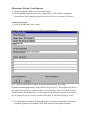
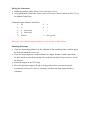
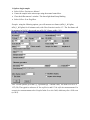
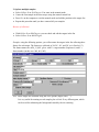
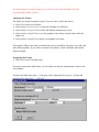
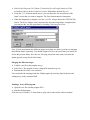
Bruker D8-GADDS
User's Manual
• Responsible:
•
•
•
•
Fabio Zürcher
tel: 642-2148 or 528-4763
email: [email protected]
Diffractometer’s mailing list: [email protected]
Diffractometer’s web-page: http://theanvil.cchem.berkeley.edu/~ gadds/
Computer:
bragg.cchem.berkeley.edu
(username: gadds, password: …….)
X-ray source:
CoKα λ=1.79026Å
If you have any doubt, ask Fabio before improvising!
Important
• Each time you touch the diffractometer, be gentle, especially with the microscope,
collimator, detector, or beam stop.
• If the shutter is open, never open the diffractometer’s windows.
• When you are moving the goniometer (manually or with the computer), beware of
collisions.
• Before starting a measurement, always check the alarm lights.
• Do not log off the computer
• The generator operating power is 45kV, 35mA.
• The generator sleeping power is 20kV, 5mA.
Measuring a Powder X-ray Diagram
• Open the program Gadds (if it is not already open).
• Set the generator’s power to the user’s setting (45kV, 35mA). Before starting the
measurement, always check the generator’s power (Collect:Goniometer:Generator)
Create a new Project
• Select New under the ProJect menu.
Example: create a project called uffa in Fabio’s personal directory.
Note: you must create the new project in your personal directory, by writing
D:\frames\username\projectname\ in the field Working Directory. The program will create a
new subdirectory called projectname in the username directory. The projectname directory
should contain a file named gadds._nc where project’s preferences are stored. You can also
use an old project (ProJect:Load), or read an old gadds._nc file (Edit:Configure:Read).
• Check whether the numbers on the gadds window are correct and whether the program
loaded the right detector's distance, flood field correction, and spatial correction.
Moving the Goniometer
• Within the program gadds: Select Collect:Goniometer:Drive.
• Using the Manual Control Box: Select Collect:Goniometer:Manual and press Shift+F1 on
the Manual Control Box.
Commands on the Manual Control Box:
1:
2θ
2:
ω
3:
φ (not in use)
4:
χ (not in use)
↑↓: to move
5:
6:
7:
x
y
z
+/-: drive speed
Emergency stop when driving the goniometer: press any key on the keyboard.
Mounting the Sample
• If you are measuring capillaries, set the collimator in the standard position (with the pin in
the hole) and mount the beam stop.
• If you are measuring plates, set the collimator at a higher distance (with the pin outside
the hole) and do not use the beam stop. Be careful that the direct X-ray beam does not hit
the detector.
• Mount the sample on the XYZ-stage.
• Move the goniometer angles (2θ and ω) at the position where you want to start the
measurement. Beware of collisions, especially with the beam stop, sample holder, or
collimator.
1. Option: single sample
• Select Collect:Goniometer:Manual.
• Center the sample in the microscope using the manual control box.
• Close the diffractometer’s window. The alarm light should stop blinking.
• Select Collect:Scan:SingleRun.
Example: using the following options, you will measure two frames (uffa0_1_001.gfrm,
uffa0_1_002.gfrm) for 10 minutes each, with 2θ as Scan Axis and ω=15°. The first frame will
be measured at 2θ=30°, the second one at 2θ=50° (Frame width = 20°).
Note: Use the symbol @ for the x, y, z positions (@ = current value). The usual Scan Axis is
1-2T (2θ). The typical ω values are 0° for capillaries and 15° for reflection measurement. For
transmission measurements select Coupled in the Scan Axis field, which stays for a 2θ/θ scan
(ω=2θ/2).
2. Option: multiple samples
• Select Collect:Scan:PickTargets. You enter in the manual mode.
• Center the first sample in the microscope using the manual control box.
• Press Esc on the computer to exit the manual mode and add the position to the targets list.
• Repeat this procedure until you have centered all your samples.
Beware of collisions!
• With Collect:Scan:EditTargets, you can check and edit the targets in the list.
• Select Collect:Scan:MultiTargets.
Example: using the following options, you will measure the targets in the list collecting three
frames for each target. The frames are collected at 2θ=30°, 40°, and 50° (ω is fixed at 15°).
The frames names are uffa1_X_00Y. gfrm with X = target number (Sequence #) and Y =
frame number (in this case: 000, 001, 002).
Note: all the targets are measured using the same options (angles, time, ….).
It is very useful for running several samples plus a blank X-ray diffractogram, which
can be used for subtracting the background caused by the air scattering.
3. Other Options
• EditRuns/MultiRuns: you can program several runs with different measuring angles, but
only one single target.
• CoupledScan:
you can perform a 2θ/θ coupled scan (ω=2θ/2) using the area
detector as a point detector.
• Add:
you can measure one frame at the current, and fixed, angles for a
specified collecting time. Note that the frame is not automatically
unwarped, therefore you have to select Process:Spatial:Unwarp
and save the unwarped file as .gfrm.
To interrupt a measurement: press Ctrl+Break.
If a measurement is currently running, you can not use the program Gadds. Open the
program Gadds-Offline, instead.
Analyzing the Frames
The frames are already unwarped (except if you use Add to collect the frame).
• Select File:Load to load a frame.
• Select Analyze:Cursors:Conic to check the 2θ angle of a reflection.
• Select Analyze:Cursors:Pixel to check the intensity measured on a pixel.
• Select Analyze:Graph:Write to save the graphics in the frames (not the frame itself) for
further use.
• Select Analyze:Graph:File to open a saved graphic on a frame.
The program Gadds is also able to calculate the percent crystallinity, the stress of a probe, and
many other properties. If you want to use these cool features, check with Fabio and read the
software manual.
Integrating the Frames
• Select File:Load to load the frame.
If you have measured a blank frame, you can subtract it from the measurement’s frame in the
Load window.
Example: the blank frame uffa1_2_000.gfrm will be subtracted (Scale factor –N) from the
measurement’s frame uffa1_1_000.gfrm.
• Select Peaks:Integrate:Chi. Choose 3-Normalized by solid angle (faster) or 5-Bin
normalized (slower) in the Normalize intensity field and the desired Step size.
• Using the 1,2,3,4 buttons and the mouse, you can adjust the size and position of the
frame’s sector that you want to integrate. The Enter button starts the integration.
• When the integration is complete, save the .raw file. Always choose the DIFFRACPlus
format. The Write window comes automatically when the integration is completed, but
you can save the .raw file again later by selecting Peaks:Integrate:Write.
Note: If your measurement has different ranges (more then one frame), you have to integrate
the different frames separately. You should assign to 2θ Start the same value you used as 2θ
End in the previous frame. Save the .raw file using always the same name, but select the
option Append (except for the first frame).
Merging the different ranges
• Load the .raw file in the program merge.
• Select Do it. The program creates a merged file named merge.out.
• Rename this file with a .raw extension.
You can also do the merging inside the Gadds program by selecting Special:System and
writing merge in the command field.
Printing a X-ray diffractogram
• Open the .raw file with the program EVA.
• Print the diffractogram
EVA has a lot of features. To learn about it, play with it and read the software manual.