1
DCell
DSC
DCell & DSC
Strain Gauge or Load Cell Embedded Digitiser
Module CANopen® – 2nd Generation
Software Version 3 onwards
User Manual
www.mantracourt.co.uk
Contents
Chapter 1 Introduction ................................................................................................................. 4
Overview ................................................................................................................................... 4
Key Features............................................................................................................................... 4
Special Facilities .......................................................................................................................... 5
Version 3 Additions and Enhancements ............................................................................................... 5
The Product Range ....................................................................................................................... 6
Which Device To Use ..................................................................................................................... 6
Additional DCell & DSC Variants Available ........................................................................................... 6
Some Application Examples............................................................................................................. 7
Chapter 2 Getting Started with the Evaluation Kit............................................................................... 8
The Evaluation Kit ........................................................................................................................ 8
Contents.................................................................................................................................... 8
Checking the Device Type............................................................................................................... 9
Connecting Up The Evaluation Kit ..................................................................................................... 9
Initial Checks .............................................................................................................................. 9
Instrument Explorer ...................................................................................................................... 9
What Can Instrument Explorer Do? .................................................................................................... 9
Installing Instrument Explorer .......................................................................................................... 9
Running the Instrument Explorer Software.......................................................................................... 10
Instrument Explorer Icon ............................................................................................................... 10
Instrument Settings...................................................................................................................... 11
Viewing Device Data .................................................................................................................... 12
Instrument Explorer Parameter List .................................................................................................. 12
Connecting a Load Cell ................................................................................................................. 13
DSJ1 Evaluation Board Sensor Connections ......................................................................................... 14
Performing A System Calibration ..................................................................................................... 15
Chapter 3 Explanation of Category Items .........................................................................................19
Information ............................................................................................................................... 19
Software Version, VER .................................................................................................................. 19
Serial Number, SERL and SERH ........................................................................................................ 19
Strain Gauge .............................................................................................................................. 19
mV/V output, MVV....................................................................................................................... 19
Nominal mV/V level, NMVV ............................................................................................................ 19
mV/V Output In Percentage Terms, ELEC ........................................................................................... 19
Temperature Value, TEMP ............................................................................................................. 19
Output Rate Control, RATE ............................................................................................................ 19
Dynamic Filtering, FFST and FFLV .................................................................................................... 20
Cell ......................................................................................................................................... 21
Temperature Compensation In Brief ................................................................................................. 21
Cell Scaling, CGAI, COFS ............................................................................................................... 21
Two Point Calibration Calculations and Examples ................................................................................. 22
Calibration Methods ..................................................................................................................... 22
Cell Limits, CMIN, CMAX ................................................................................................................ 23
Linearisation In Brief.................................................................................................................... 23
System ..................................................................................................................................... 23
System Scaling, SGAI, SOFS ............................................................................................................ 23
Example of calculations for SGAI and SOFS ......................................................................................... 24
System Limits, SMIN, SMAX............................................................................................................. 24
System Zero, SZ .......................................................................................................................... 25
System Outputs, SYS, SOUT ............................................................................................................ 25
Reading Snapshot, SNAP, SYSN ........................................................................................................ 25
Control..................................................................................................................................... 25
Shunt Calibration Commands, SCON and SCOF ..................................................................................... 25
Digital Output, OPON and OPOF ...................................................................................................... 25
Flags ....................................................................................................................................... 25
Diagnostics Flags, FLAG and STAT .................................................................................................... 25
Latched Warning Flags (FLAG)......................................................................................................... 25
1
Mantracourt Electronics Limited DCell & DSC CANopen® User Manual
Meaning and Operation of Flags....................................................................................................... 26
Dynamic Status Flags (STAT)........................................................................................................... 27
Meaning and Operation of Flags....................................................................................................... 27
Output Update Tracking ................................................................................................................ 27
User Storage .............................................................................................................................. 28
USR1…USR9 ............................................................................................................................... 28
Reset ....................................................................................................................................... 28
The Reset command, RST .............................................................................................................. 28
WARNING: Finite Non-Volatile Memory Life......................................................................................... 28
Chapter 4 The Readings Process ....................................................................................................29
Flow diagram ............................................................................................................................. 29
Cell and System Scaling................................................................................................................. 30
Calibration Parameters Summary and Defaults .................................................................................... 31
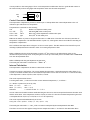
Chapter 5 Temperature Compensation ............................................................................................32
Purpose and Method of Temperature Compensation .............................................................................. 32
Temperature Module Connections and Mounting (DTEMP) ....................................................................... 32
Control Parameters...................................................................................................................... 33
Internal Calculation ..................................................................................................................... 33
The Temperature Measurement....................................................................................................... 34
How to Set Up a Temperature Compensation ...................................................................................... 34
Parameter Calculations................................................................................................................. 35
Chapter 6 Linearity Compensation .................................................................................................36
Purpose and Method of Linearisation ................................................................................................ 36
Control Parameters...................................................................................................................... 36
Internal Calculation ..................................................................................................................... 36
How to Set Up Linearity Compensation.............................................................................................. 37
Parameter Calculations and Example ................................................................................................ 37
Chapter 7 Self-Diagnostics ............................................................................................................39
Diagnostics Flags......................................................................................................................... 39
Diagnostics LED .......................................................................................................................... 39
Chapter 8 CANopen® Communication Protocol ..................................................................................40
CANopen® Features Support Summary .............................................................................................. 40
Object Dictionary Summary............................................................................................................ 41
Error Management ....................................................................................................................... 42
Communications Controls .............................................................................................................. 42
Data Type Conversions and Rounding ................................................................................................ 43
Chapter 9 Object Dictionary .........................................................................................................44
Communications Profile Area.......................................................................................................... 44
Device Description and Communication Specific................................................................................... 44
Transmit PDO Operation Specific ..................................................................................................... 45
Transmit PDO Mapping Specific ....................................................................................................... 46
Manufacturer Specific Area ............................................................................................................ 47
Chapter 10 Installation ................................................................................................................48
Before Installation....................................................................................................................... 48
Physical Mounting........................................................................................................................ 48
Electrical Protection .................................................................................................................... 48
Moisture Protection ..................................................................................................................... 48
Soldering Methods ....................................................................................................................... 49
Power Supply Requirements ........................................................................................................... 49
Cable Requirements ..................................................................................................................... 49
Strain Gauge input (DSC) ............................................................................................................... 49
Power and Communication............................................................................................................. 49
Temperature Sensor..................................................................................................................... 49
Identifying Strain Gauge Connections ................................................................................................ 50
DCell Input Connections ................................................................................................................ 50
DSC Input Connections .................................................................................................................. 50
Identifying Bus-End Connections ...................................................................................................... 50
DCell Bus Connections .................................................................................................................. 50
Mantracourt Electronics Limited DCell & DSC CANopen® User Manual
2
DSC CAN Versions-Bus Connections ................................................................................................... 51
Strain Gauge Cabling and Grounding Requirements ............................................................................... 51
DCell Strain Gauge Wiring .............................................................................................................. 51
DCell Strain Gauge Wiring Arrangement ............................................................................................. 51
Key Requirements ....................................................................................................................... 51
DSC Strain Gauge Cabling Arrangement ............................................................................................. 52
Key Requirements ....................................................................................................................... 52
Communications Cabling and Grounding Requirements........................................................................... 53
DCell Power and Communications Wiring ........................................................................................... 53
DCell Bus-End Arrangement ............................................................................................................ 53
DSC4 Versions- Power and Communications Wiring................................................................................ 54
DSC4 Versions-Bus-End Arrangement ................................................................................................. 54
Key Requirements ....................................................................................................................... 54
Suitable Cable Types .................................................................................................................... 54
DCell/DSC CAN Bus Cable .............................................................................................................. 54
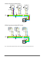
CAN Bus Connections for Multiple DCells ............................................................................................ 55
CAN Bus Connections for Multiple DSC Versions.................................................................................... 55
Key Requirements ....................................................................................................................... 56
Bus Layout and Termination ........................................................................................................... 56
Loading .................................................................................................................................... 56
Strain Gauge Sensitivity Adjustment (DSC ONLY) .................................................................................. 56
Identifying the DSC ‘Rg’ Resistor ..................................................................................................... 56
Chapter 11 Troubleshooting .........................................................................................................58
LED Indicator ............................................................................................................................. 58
No Communications ..................................................................................................................... 58
Bad Readings ............................................................................................................................. 58
Unexpected Warning Flags ............................................................................................................. 59
Problems with Bus Baud Rate.......................................................................................................... 59
Recovering a ”lost” DCell/DSC ........................................................................................................ 59
Resetting to default ID.................................................................................................................. 59
First Command ........................................................................................................................... 59
Second Command ........................................................................................................................ 59
Chapter 12 Specifications.............................................................................................................60
Technical Specifications DSC/DCELL High Stability................................................................................ 60
Technical Specifications DSC/DCell Industrial Stability........................................................................... 61
Mechanical Specification for DSC ..................................................................................................... 62
Mechanical Specification for DCell ................................................................................................... 62
CE Approvals.............................................................................................................................. 62
Warranty .................................................................................................................................. 63
3
Mantracourt Electronics Limited DCell & DSC CANopen® User Manual
Chapter 1 Introduction
This chapter provides an introduction to DCell/DSC products, describing the product range, main features and
application possibilities.
Overview
The DCell and DSC products are miniature, high-precision Strain Gauge Converters; converting a strain gauge sensor
input to a CANopen® output. They allow multiple high precision measurements to be made over a low-cost 2-wire
link. Outputs can be accessed directly by PLCs or computers, or connected via various types of network, all without
compromising accuracy.
The device is configurable using a CANopen® configuration tool.
Key Features
Ultra-miniature
The DCell ‘puck’ format can be fitted inside most load cell pockets, and similar restricted spaces. The DSC cards
are similarly very small, optimised for mounting as a component onto custom PCBs.
High-precision Industrial Version.
25ppm basic accuracy (equates to 16 bit resolution)
High-precision High Stability
5ppm basic accuracy (equates to 18 bit resolution) with comparable stability – far exceeds standard instrument
performance.
Low-power
Low-voltage DC supply (5.6V min), typically 40mA for RS485 and 52mA for RS232 (including 350R strain gauge).
Adjustable sensitivity
Configured for standard 2.5mV/V full-scale strain gauges as supplied.
A single additional resistor configures the input between 0.5 and 100 mV/V full-scale.
Temperature sensing and compensation (optional)
An optional temperature sensor module is available and advanced 5-point temperature-compensation of
measurement.
Linearity compensation
Advanced 7-point linearity compensation.
CAN Output
Lower-cost cabling, improved noise immunity, and longer cable runs with no accuracy penalty.
Device addressing allows up to 127 devices on a single bus, drastically reducing cabling cost and complexity.
Two-way communications allow in-situ re-calibration, multiple outputs and diagnostics.
No separate measuring instruments needed.
Digital calibration
Completely drift-free, adjustable in-system and/or in-situ via standard communications link.
Two independent calibration stages for load cell-and-system-specific adjustments.
Programmable compensation for non-linearity and temperature corrections.
Calibration data is also transferable between devices for in-service replacement.
Self-diagnostics
Continuous monitoring for faults such as strain overload, over/under-temperature, broken sensors or unexpected
power failure.
All fault warnings are retained on power-fail.
Mantracourt Electronics Limited DCell & DSC CANopen® User Manual
4
Special Facilities
Output Capture Synchronisation
A single command instructs all devices on a bus to sample their inputs simultaneously, for synchronised data
capture.
Output Tare Value
An internal control allows removal of an arbitrary output offset, enabling independent readings of net and gross
measurement values.
Dynamic Filtering
Gives higher accuracy on stable inputs, without increased settling time.
Programmable Output Modes
Output rate control enables speed/accuracy trade-off.
ASCII output version provides decimal format control and continuous output mode for ‘dumb terminal’ output.
Unique Serial Number
Every unit carries a unique serial-number tag, readable over the communications link.
Communications Error Detection
CAN transmit and receive error counts along with CAN bus status can be read from the device.
External Temperature Sensing (optional)
An external temperature module for improved accuracy (especially tracking changing temperature conditions).
Software Reset
A special communications command forces a device reboot, as a failsafe to ensure correct operation.
Version 3 Additions and Enhancements
The following are an outline only more detail will be found further on in this manual
DCell
•
•
•
Easy mounting via a 2mm screw
Connection via solder holes to either side of PCB
Lower profile, dual PCB construction
DSC
•
•
Additional I/O
Easier shielding connection at load cell connector end
DCell & DSC
• Bit rates to 1 Mbps
• Higher sampling rate. Sampling to 200Hz can now be achieved. Also more sampling rates are available as
follows 1, 2, 5, 10, 20, 50, 60, 100 & 200Hz.
• Lower cost. With new technology and further use of miniaturisation the cost is now lower.
• Real mV/V calibration. Instead of % full scale the base measurement is in mV/V and is factory calibrated to
within 0.1%. the % of FS output “ELEC” is still available.
• Extreme Noise Immunity, 5 x heavy industrial level.
• Diagnostics LED. An LED is used to indicate that the device is powered and working correctly. The LED is also
used to indicate which protocol the device is.
• Remote shunt cal. A 100K 1% 50ppm/Deg C resistor can be switched across the bridge to allow load cell
integrity to be established.
• Peak & Trough Measurements. Added to allow the faster rates to hold a peak or trough readings. These are
stored in volatile memory & are therefore reset on power up.
• Programmable dynamic filtering. The filtering is the same as used on Version 2 but with the advantage of
being able to set the characteristics using the communications.
• Wide Operating Voltage. The operating voltage is now 5.5 to 18V allowing the device to be powered from a
wider range of available system supplies.
• DC Excitation. DC excitation has now been employed allowing longer cable lengths for the load cells which is
particularly useful for DSC. This is a 4-wire measurement.
5
Mantracourt Electronics Limited DCell & DSC CANopen® User Manual
•
Scaling implementation has been changed for both “CELL” and “SYS”. The gain is applied before the offset
thus following the more standard approach. This allows for an offset change to be made easily as the offset
is not a component of gain.
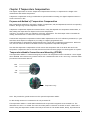
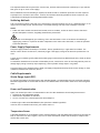
The Product Range
Devices are available in two physical formats:
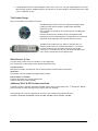
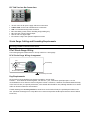
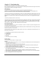
The DCell (puck) products consist of a Digital Strain Gauge Signal
Conditioner with CAN bus output in double sided component
population format.
This is suitable for installation in very small spaces, including load
cell pockets.
External connections are made by wiring to through hole pads.
Mounting is via a 2mm mounting hole to accept M2 screw or American
equivalent #0-80. Important Note: DO NOT USE #2 screw size.
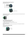
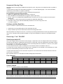
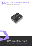
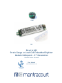
The DSC (card) products are very similar to the DCell but in a
different physical form for mounting stand-alone or on a board.
External connections are via header pins which can plug into
connectors, or be soldered to wires or into a host PCB. DSC has an
open collector output and volt free digital input.
Which Device To Use
It is important to select the correct product for your application.
First choose DCell or DSC based on your physical installation needs
Common Features
Both physical formats offer identical control and near-identical measurement performance
Differences
Only the DSC (card) is available with digital Input & output.
Special Aspects To Consider
The DCell fits neatly into a strain gauge pocket
The DSC lends itself to PCB mounting
Additional DCell & DSC Variants Available
A separate variant is available with RS232 or RS485 output. Refer to DCell & DSC CAN - 2nd Generation - Manual.
(These variants are sufficiently different to require their own manuals)
The following order codes are supported by an earlier version manual ‘DCell & DSC Version 2’
DLCPKASC, DLCPKMAN, DLCPKMOD, DSC2AS, DSC2MA, DSC2MB, DSC4AS, DSC4MA, DSC4MB
Mantracourt Electronics Limited DCell & DSC CANopen® User Manual
6
Some Application Examples
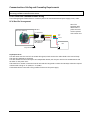
Simple Distributed Measurement
Pressure loads are taken at a number of keys points in a manufacturing process, distributed over a large area.
Each pressure sensor contains a DCell unit, and all the sensors are connected by a single cable carrying power and
CAN communications. A central PC allows continuous display, monitoring and logging of all values from a central
control room. This displays a control-panel and current display window, and logs information to an Excel
spreadsheet for future analysis.
Further monitoring checks and displayed information can easily be added when required to the system where up to
127 ‘nodes’ can be installed.
Low Cost Dedicated Weighing Station
A basic load cell weighing-pad device has a cable leading to a wall mounted weight display.
Digital Load Cell
Load cell products are offered with a high-precision digital communications option.
A DCell is fitted into the gauge pocket of each load cell in manufacture. During product testing, each unit undergoes
a combined load test and temperature cycle. Each unit is then programmed with individually calculated gain, offset,
linearity and temperature compensation tables. All units perform to a very tight specification without the use of any
trimming components.
High Reliability Load sensing
A road bridge has a dedicated load monitoring and active control computer system. System calibration adjustments
are only established during construction, so sensors must be replaceable without recalibration.
Each load monitoring point has a digital load cell fitted, with calibration values set during construction. Selfdiagnostics aid detection of failures.
When a failed load cell is replaced it will produce identical force measurements. The old load cell set-up data
values are programmed into the separate user-level calibration store in the unit, to produce an identically
performing replacement.
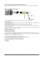
Load Balance Monitor
A lorry loading weighpoint monitors left/right load balance and sounds a warning if loading is too uneven for safety.
A drive-on weighing platform is provided with load cells at each of four corners. Each cell is wired to a DSC unit, and
these are cabled to a 3rd party LCD display and control unit, producing a complete turnkey system. A digital I/O card
is wired to the same bus to control the warning alarm. Application software running on the control unit provides a %
left/right balance readout with a graphical tipping display, and a total weight indication.
The balance indication is calculated by comparing the different corner readings. If it exceeds a programmed limit, a
command to the I/O card turns the relay on.
Total weight is calculated by summing the individual results mathematically.
Automatic re-zeroing occurs when the total is near zero for more than a few seconds.
A control button enables a set-up mode for recalibration (protected by operator password), which displays individual
readings and total. Corner compensation can be checked by observing the changing total as a weight is moved
around. Simple button presses control two point recalibration for any cell.
7
Mantracourt Electronics Limited DCell & DSC CANopen® User Manual
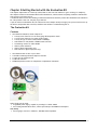
Chapter 2 Getting Started with the Evaluation Kit
This chapter explains how to connect up a DCell/DSC for the first time and how to get it working. For simplicity,
this chapter is based on the standard DCell/DSC Evaluation Kit, which contains everything needed to communicate
with a puck or card from your PC.
It is advised that first time users wishing to familiarise themselves with the product use the Mantracourt Evaluation
Kit. This provides a low cost, easy way to get started.
If you do not have an Evaluation Kit, the instructions in this chapter mostly still apply, but you will need to wire up
the device (and possible bus-converter) and have some means of communicating with it.
The Evaluation Kit
Contents
• An Evaluation PCB (DSJ1) which comprises of
• A 8 way screw connector for the strain gauge & Temperature sensor
• A 5 way screw connector for power & CAN comms
• A 9 way ‘D’Type for direct CAN (limited to 500Kbps)
• Link headers for CAN, RS232 or RS485 comms selection
• Terminating resistor for CAN & RS485
• LED for power indication
• LED for digital output (DSC only)
• Push Switch for digital input (DSC only)
•
•
•
•
•
An Evaluation DCell or DSC of your choice
A CD ROM containing Instrument Explorer software
A 9 way ‘D’Type extension lead
A USB-CAN converter
DTEMP temperature sensor for temperature compensation evaluation
Other Things you will need.
• A regulated power supply, capable of providing 5.6 –18V at 100mA
• A PC running Windows 98 or above, with a spare USB port and 45Mb free disk space
and, ideally
• A strain gauge, load cell or simulator, 350-5000 ohms impedance.
Mantracourt Electronics Limited DCell & DSC CANopen® User Manual
8
Checking the Device Type
For a DCell, the Product Code is one of the following 2 types
DLCSCOP
Industrial Stability CANopen® output
DLCHCOP
High Stability CANopen®® output
For a DSC card, the Product Code is one of the following 2 types
DSCSCOP
Industrial Stability CANopen® output
DSCHCOP
High Stability CANopen® output
The CAN bus Identifier ID of a New DCell/DSC device is factory set to 127
This can be changed using the CANopen® command at Index 2000 subindex 0.
Connecting Up The Evaluation Kit
Power is supplied to the DSJ1 via the 5 way connector (J1). This is connected to a supply set between 5.6v and 18v
DC. The red wire being positive and the black negative. The CAN is connected using the 9 way D-type extension lead
to J3 and to the USB-CAN converter.
Ensure LK1 & LK5 are set to “CAN/RS485”. Fit LK2 which terminates the CAN bus.
Switch on, the Green Power LED of the DSJ1 should be on.
Initial Checks
With no load cell connected The LED of the DCell or DSC should flash OFF for 100ms every 0.5s.
Note: If a Load cell is connected and there are no errors then the LED will Flash ON for 100mS then Off for the
above period. This being the normal healthy state.
Another check that the device is working okay is by noting the current drawn from the supply, this should be about
40mA.
Instrument Explorer
Instrument Explorer is Mantracourts own communication interface for our range of standard products. It provides
communications drivers for the DCell/DSC products. A complimentary copy is provided on CD-ROM with the
DCell/DSC Evaluation Kit. Instrument Explorer can also be downloaded from Mantracourts website.
http://www.mantracourt.co.uk/software/Instrument_Explorer
Instrument Explorer is a software application that enables communication with Mantracourt Electronics
instrumentation for configuration, calibration, acquisition and testing purposes.
The clean, contemporary interface allows full customisation to enable your Instrument Explorer to be moulded to
your individual requirements.
What Can Instrument Explorer Do?
•
•
•
•
•
Save and restore customisable user workspace
Read and Write individual instrument parameters
Save and restore parameter configurations
Log data to a window or file
Perform calibration and compensation
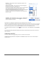
Installing Instrument Explorer
Install the Instrument Explorer software by inserting the CD in the CD ROM drive. This should start the ‘AutoRun’
process, unless this is disabled on your computer.
(If the install program does not start of its own accord, run SETUP.EXE on the CD by selecting ‘Run’ from the ‘Start
Menu’ and then entering D:\SETUP, where D is the drive letter of your CD-ROM drive).
9
Mantracourt Electronics Limited DCell & DSC CANopen® User Manual
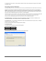
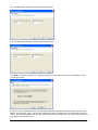
The install program provides step-by-step instructions. The software will install into a folder called
InstrumentExplorer inside the Program Files folder. You may change this destination if required.
Shortcut icons can be created on your desktop and shortcut bar. After installation you may be asked to restart the
computer. This should be done before proceeding with communications.
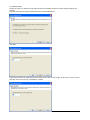
When given the option to install IXXAT CAN drivers ensure these are selected, which is the default.
Running the Instrument Explorer Software
Having installed Instrument Explorer you can now run the application, which the rest of this chapter is based
around.
From the Windows ‘Start’ button, select Programs, then Instrument Explorer or click on the shortcut on your
desktop.
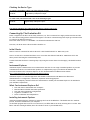
Instrument Explorer Icon
The application should open and look like the following shield shot.Instrument Explorer Window
Mantracourt Electronics Limited DCell & DSC CANopen® User Manual
10
The layout of Instrument Explorers Window and child windows allows the user full customisation to their
requirements. If the application show a different arrangement of child windows than the above shield shot then
using then load one of the default workspaces as follows:
Click File on the menu and select Open Workspace. From the file dialogue window select Layout – Standard.iew.
This will ensure your application layout matches this document.
A list of available instruments is displayed in the Select Instrument pane of Instrument Explorer. Select the relevant
device by clicking on the required device icon under the MantraCAN heading.
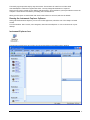
Instrument Settings
CANopen®
•
•
•
•
Select the ID. The factory default is 127 decimal (7F HEX).
Select the baud rate to which the device is set. The factory default is 125KB.
Select the ID type. Default is 11Bit (standard note extended not supported)
Now click the ‘OK’ button…
The above assumes factory defaults. If your device is known to have different settings use these instead of the ones
stated above.
11
Mantracourt Electronics Limited DCell & DSC CANopen® User Manual
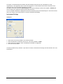
Viewing Device Data
The following main parameter list should now appear in the central pane.
Instrument Explorer Parameter List
When an instrument has been selected from the Select Instrument Window this Parameter List window will become
populated.
The parameters and commands which are available for the selected device will appear in this list in a structured
hierarchic manner enabling the user to expand or contract categories by clicking the and buttons on the left of
the list.
There are four types of parameters and commands:
Read/write Numeric – These parameter values are displayed in the right
hand column and can be edited by clicking the value.
The value can then be changed and pressing the Enter key or moving away
from the edited value will cause the new value to be written to the
device. There are no checks on the data entered and it is up to the user
to enter the correct data.
Mantracourt Electronics Limited DCell & DSC CANopen® User Manual
12
Read-Only – These parameter values are displayed ‘greyed out’ and
cannot be changed.
Read/write Enumerated – These parameters can only be changed by
selecting the new value from a drop down list.
Clicking in the right hand column will display a down arrow button which
when clicked will display the parameter value options in a list.
Note that all enumerated data (apart from on/off) will be displayed with
a numeric value, hyphen then the description of the value.
The numeric value is the value of the parameter and the description is
just there to help.
Commands – These commands have ‘Click to execute…’ displayed in the
right hand column. Clicking here will display a
button. Click this to
issue the command to the device.
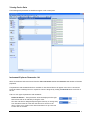
As parameters are changed the communications traffic is displayed in the Traffic Pane.
If any errors occur these will be shown in red in the Error Pane. Once an error occurs it will need to be reset before
any more communications can take place. Reset errors by either right-clicking the Error Pane and selecting Reset
Errors from the pop-up menu or select the Communications menu and click the Reset Errors item.
To manually refresh the parameter list click the
menu.
button on the toolbar or select Sync Now from the Parameters
Now you have successfully established communications with your evaluation device the next step is to perform a
simple calibration.
Connecting a Load Cell
You can now connect a strain gauge bridge, load cell or simulator to the DCell/DSC.
A suitable strain gauge should have an impedance of 350-5000ohms and (at least for now) a nominal output of
around 2.5mV/V.
13
Mantracourt Electronics Limited DCell & DSC CANopen® User Manual
DSJ1 Evaluation Board Sensor Connections
Next Instrument Explorer will set to automatically update dynamic parameters from the device so that
we can see values as SYS changing on the shield. To do this either click the
button on the toolbar or
click on the Parameters menu and select the Auto Sync item. Note that these options toggle so be sure
to leave your selection in the active state.
From the Parameter List click the
as follows:
next to the System heading to expand this level. The Parameter List should look
This now exposes more levels that can be expanded as
required by clicking the next to the heading name.
Dynamic values (such as SYS and SRAW) will now be updating in real-time from the device.
Once you have connected the load cell, you should see ‘believable’ output values, in the “SYS” parameter displayed
in the parameter list pane. These values should correspond to mV/V assuming the device is in it’s factory default
state.
Mantracourt Electronics Limited DCell & DSC CANopen® User Manual
14
For diagnostics the device has a of flags. Which is dynamic and will cause an Emergency Telegram to be broadcast
on change of state.
Performing A System Calibration
The values obtained so far are in mV/V units, these are factory calibrated and fixed to within about 0.1% accuracy.
The device also contains two separate user-adjustable calibration parameter groups, these are termed Cell and
System. Cell being used to convert from mV/V to a force and System to convert this force to required engineering
units. We shall being using System for the following exercise where we rescale the output value to read in units of
your choice, and to calibrate precisely to your load cell / system hardware.
Instrument Explorer provide ‘Wizards’ to allow quick and simple calibration operations to be undertaken without the
use of a calculator. Wizards can be activated by simply selecting the required item from the Wizard menu.
Since we are now calibrating at system level we have a choice of two calibration methods:
Sys Calibration Table – This technique is used when a manufacturers calibration document is available for the
connected strain gauge. This normally gives mV/V to engineering unit values.
Sys Calibration Auto – This technique is used when the input can be stimulated with real input values. For example
you have access to test weight / forces.
We will now describe each of these techniques with an example.
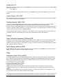
Sys Calibration Table
A 10 tonne load cell manufacturer gives the following data:
mV/V output
2.19053
-0.01573
Force
10 tonne
0 tonne
Start the wizard by selecting Sys Calibration Table from the Wizard menu
15
Mantracourt Electronics Limited DCell & DSC CANopen® User Manual
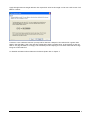
Click the Next button and enter the low values as shown below.
Click the Next button and enter the high values as shown below.
Click Next the following window will be displayed showing the calibrated SYS value which is dependent on the
current input values.
The device is now calibrated. However you may find SYS has been ‘clamped’ if the resultant SYS is greater than
SMAX or less than SMIN. If this is the case then change these values to suitable limits. In this example we may set
SMIN to –0.5 (tonne) and SMAX to 12.0 (tonne). This would then provide clamping of SYS to these values and also a
flags being set in FLAG and STAT.
Mantracourt Electronics Limited DCell & DSC CANopen® User Manual
16
Sys Calibration Auto
Assume we require to calibrate for Kg output and we have available a known accurate 10 Kg and 100 Kg test
weights.
Start the wizard by selecting Sys Calibration Auto from the Wizard menu
Click Next.
Apply the low known test weight and enter the required SYS value for this weight. In this case it will be 10 as we
want the units of SYS to be Kg. Click Next to continue
17
Mantracourt Electronics Limited DCell & DSC CANopen® User Manual
Apply the high known test weight and enter the required SYS value for this weight. In this case it will be 100. Click
Next to continue.
The device is now calibrated. However you may find SYS has been ‘clamped’ if the resultant SYS is greater than
SMAX or less than SMIN. If this is the case then change these values to suitable limits. In this example we may set
SMIN to –0.5 (Kg) and SMAX to 110.0 (Kg). This would then provide clamping of SYS to these values and also a flags
being set in FLAG and STAT.
For detailed information about calibration calculations please refer to chapter 3.
Mantracourt Electronics Limited DCell & DSC CANopen® User Manual
18
Chapter 3 Explanation of Category Items
Instrument Explorer shows the categories to which parameters and generated variables belong. This provides a
convenient method for describing the functionality and purpose of each. The categories can be seen from
Instrument Explorers Parameter List pane and are as follows.
Information
Reports the current version of the devices software and the devices unique serial number. Note that VERSION is the
read able item derived from the devices internal value of VER and SerialNumber is derived from SERL and SERH.
Software Version, VER
The VER parameter (read-only byte) returns a value identifying the software release number, coded as 256*(majorrelease)+(minor-release) , where MSB of VER is major release and LSB of VER is minor release
Eg. current version 3.1 returns VER=769 (256 x 3 + 1)
Serial Number, SERL and SERH
SERL and SERH are read-only integer parameters returning the device serial-number.
This is decoded as = 65536*SERH + SERL.
The VisualLink/Instrument Explorer software drivers include a convenience ‘Serial Number’ property that
automatically does this.
Strain Gauge
This is where the measurement process starts. If the optional temperature module is fitted then TEMP will display
actual temperature in Degree C. Otherwise TEMP will display 125 Degree C.
RATE is the parameter that selects measurement cycle update rate.
mV/V output, MVV
MVV is the factory calibrated mV/V output and it is this value that all other measurement output values are derived
from. Factory calibration is within 0.05%.
Nominal mV/V level, NMVV
This is used to represent the nominal mV/V value representing 100% of full scale. This value is used solely for the
generation of ELEC. It is factory set for 2.5mV/V. If the electronic gain is adjusted by changing the gain resistor
then if ELEC is used NMVV value must be changed to represent the new nominal mV/V.
mV/V Output In Percentage Terms, ELEC
This is mainly for backwards compatibility with Version 2. It is the mV/V value represented in percentage terms,
100% being the value set by NMVV.
Temperature Value, TEMP
If the optional temperature module is fitted, DTEMP then TEMP will display actual temperature in Degree C.
Otherwise TEMP will display 125 Degree C. TEMP is used by the temperature compensation. See chapter 5
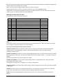
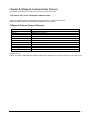
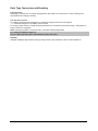
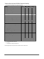
Output Rate Control, RATE
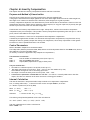
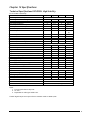
The RATE parameter is used to select the output update rate, according to the following table of values –
RATE value
update rate (readings per
second)
0
1
1
2
2
5
3
10
4
20
5
50
6
60
7
100
8
200
The default rate is 10Hz (RATE=3): The other settings give a different speed/accuracy trade-off.
Invalid RATE values are treated as if it was set to 3.
19
Mantracourt Electronics Limited DCell & DSC CANopen® User Manual
The underlying analogue to digital conversion rate is 1627Khz. These results are block averaged to produce the
required output rate.
To Change The Output Rate
1. Set RATE to the new value
2. Click on the ‘RST’ button to reboot the device
3. Wait for one second for the reset procedure to complete and measure cycle to start
With RATE set to 0, you should be able to see the SYS update rate slow to once a second, and the noise level should
also noticeably decrease.
All the main-reading output values are updated at this rate. Rate does not change the rate at which temperature
output TEMP is updated.
Important Note:
For A RATE of 8 (200Hz) Temperature compensation and Linearisation cannot be used due to Calculation time
required.
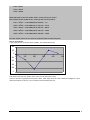
Dynamic Filtering, FFST and FFLV
The Dynamic filter is basically a recursive filter and therefore behaves like an “RC” circuit. It has two user settings,
a level set in mV/V by FFLV and a maximum number of steps set by FFST, maximum value FFST can be is 255. If a
difference between a new input value (RMVV) and the current filtered value (MVV) is greater than FFLV then the
fractional amount of the new reading added to the current reading is reset to 1, that is to say that output of the
filter will be equal to the new input reading. If the difference is less than FFLV then the fractional amount added is
incremented until it reaches the maximum level set by FFST.IE if FFST = 10 then after a step change the fractional
part of a new reading is incremented as follows
1/1, 1/2, 1/3, 1/4, 1/5, 1/6…. 1/10, 1/10, 1/10
This allows the Filter to respond rapidly to a fast moving input signal.
With a step change, which does not exceed FFLV, the calculated new filtered value can be calculated as follows
New Filter Output value = Current Filter Output Value + ((Input Value - Current Filter Output Value) / FFST)
The time taken to reach 63% of a step change input (which is less than FFLV) is the frequency at which values are
passed to the dynamic filter, set in RATE, multiplied by FFST.
The table below gives an indication of the response to a step input less than FFLV.
Update Rate is 1/table value of RATE see Chapter 3 Output Rate Control.
% Of Final Value
63%
1%
0.1%
Time To settle
Update Rate * FFST
Update Rate * FFST * 5
Update Rate * FFST * 7
For example, If RATE is set to 7 = 100Hz = 0.01s and FFST is set to 30 then the time taken to reach a % of step
change value is as follows.
% Of Final Value
Time To settle
63%
0.01 x 30 = 0.3 seconds
1%
0.01 x 30 x 5 = 1.5 seconds
0.1%
0.01 x 30 x 7 = 2.1 seconds
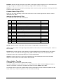
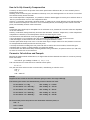
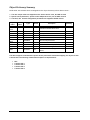
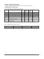
The following table shows the number of updates x FFST and the error % New Filter Output value will differ from a
constant Input Value.
x FFST
% Error
1
36.7879441
2
2
13.5335283
2
Mantracourt Electronics Limited DCell & DSC CANopen® User Manual
20
3
4
5
6
7
8
9
10
11
12
13
14
15
16
17
18
19
20
4.97870684
1.83156389
0.67379470
0.24787522
0.09118820
0.03354626
0.01234098
0.00453999
0.00167017
0.00061442
0.00022603
0.00008315
0.00003059
0.00001125
0.00000414
0.00000152
0.00000056
0.00000021
Remember that if the step change in mV/V is greater than the value set in FFLV then
New Filter Output value = New Input Value.
And the internal working value of FFST is reset to 1, being incremented each update set by RATE until it reaches
the user set value of FFST.
Cell
Provides the level where the integration between the DCell/DSC and the strain gauge bridge takes place. Features
include, when the optional temperature module is fitted, 5-point temperature compensation to produce a
temperature compensated value CMVV. Scaling using a gain and offset, CGAI and COFS respectively, producing a
value known as CRAW. Linearisation, using up to 7-points, producing the final output from this section known as
CELL. Over load and under load values can be set in CMIN & CMAX to alert the user of forces less or greater than
the integrator has intended the unit to be operated. These features allow the output CELL to be in force units which
can be used by ‘System’ to convert to units of weight.
Temperature compensation and linearisation are covered in detail in their own chapters.
Temperature Compensation In Brief
When the optional temperature hardware module DTEMP is connected the temperature compensation is available.
The temperature compensation facility can remove the need for the fitting of compensation resistors to the strain
gauges. This compensation can apply for gain and offset with up to 5 temperature points.
The input for the temperature compensation is MVV and the output from the process is CMVV. If not temperature
compensation is invoked the CMVV is equal to MVV
Temperature compensation cannot be used at RATE of 8 (200Hz)
A Detailed explanation is given in chapter 5
Cell Scaling, CGAI, COFS
The temperature compensated value CMVV is scaled with gain and offset using CGAI and COFS respectively. The
gain is applied first and the offset the subtracted. This would be used to give a force output in the chosen units, this
output being termed CRAW.
CRAW = (CMVV X CGAI) – COFS
21
Mantracourt Electronics Limited DCell & DSC CANopen® User Manual
Two Point Calibration Calculations and Examples
Examples are given here for two point calibration, as this is by far the most common method.
Cell Calibration
The scaling parameters are CGAI and COFS
CGAI is in cell-units per mV/V’
COFS is in cell units
The cell output calculation is (in the absence of temperature and linearity corrections) –
CRAW = (CMVV × CGAI) – COFS
If we have two electrical-output (MVV) readings for two known force loads, we can convert the output to the
required range. So if –
test load = fA CMVV reading = cA
test load = fB CMVV reading = cB
– then calculate the following gain value
CGAI = (fB – fA) / (cB – cA)
and the offset is
COFS = (cA x CGAI) – fA
The outputs should then be CELL = fA, fB true force values, as required.
Calibration Methods
There are a number of ways of establishing the correct control values.
Method 1 - Nominal (data sheet) Performance Values
This is the simplest method, where the given nominal mV/V sensor output is used to calculate an approximate value
for CGAI.
Example.
A 50 kN load cell has nominal sensitivity of 2.2mV/V full-scale.
So to get 50.0 for an input of 2.2mV/V, we set CGAI to 50/2.2≈
≈22.7273. This assumes the output for 0kN is
0mV/V.
Method 2 - Device Standard (Calibration) Values
With some load cells you may have a manufacturer’s calibration document. This gives precise cell-output gain and
offset specifications for the individual cell. These values can be used to set the SGAI and SOFS values to be used.
Example.
A 10 tonne load cell has a calibration sheet specifying 2.19053mV/V full-scale output, and -0.01573mV/V
output offset.
CGAI is set to 10 / (2.19053- -0.01573) ≈ 4.532557.
COFS is set to –0.01573 x 4.532557≈
≈ -0.0071297
NOTE:
Methods 1 and 2 require no load tests. This means that systematic installation errors cannot be removed, such as
cells not being mounted exactly vertical. The accuracy is also limited by the DCell/DSC electrical calibration
accuracy, which is about 0.1%.
The remaining methods require testing with known loads, but are therefore inherently more reliable in practice, as
they can remove unexpected complicating factors relating to installation.
Method 3 - Two-Point Calibration Method
This is a simple in-system calibration procedure, and probably the commonest method in practice (as in the previous
example).
Two known loads are applied to the system, and reading results noted, then calibration parameters are set to
provide exactly correct readings for these two conditions.
Mantracourt Electronics Limited DCell & DSC CANopen® User Manual
22
E.G. a 10kN (1-tonne) load cell has a CELL reading of +0.120721mV/V with no load, and –2.21854mV/V with a
known 100Kg test-weight.
To calibrate this to read in a –1.0 to +1.0 tonne range,
Calculate CGAI as 0.1 / (2.21854 - +0.120721) = 0.047669.
Set COFS= 0.120721 x 0.047669 = 0.005755.
Method 4 - Multi-point Calibration Test
For ultimate accuracy to a whole series of point measurements may be taken to determine the best linear scaling of
input output: Effectively, a ‘best line’ through the data is then chosen, and the calibration is set up to follow the
line.
Testing of this sort is also used to establish linearity corrections, and similar tests at different temperatures are
used to set up temperature compensation (see Chapters on Temperature Compensation and Linearity
Compensation).
Note: Instrument Explorer provides “wizards” for easy calibration of the Cell stage. There are two wizards, ‘Cell
Calibration Auto’ and ‘Cell Calibration Table’ these can be found under the menu item “Wizards”.
Cell Limits, CMIN, CMAX
These are used to indicate that the desired maximum and minimum value of CRAW have been exceeded. They are
set in Force units. On CRAW being greater than the value set in CMAX the CRAWOR flag is set in both FLAG and
STAT, the value of CRAW is also clamped to this value. On CRAW being less than the value set in CMIN the CRAWUR
flag is set in both FLAG and STAT, the value of CRAW is also clamped to this value.
Linearisation In Brief
Linearisation allows for any non-linearity in the strain gauge measurement to be removed. Up to 7 points can be set
using CLN. The principle of operation is that the table holds a value at which an offset is added. The point in the
table that refer to CRAW are named CLX1..CLX7. The offsets added at these point are named CLK1.. CLK7 and are
set in thousandths of a cell unit. The output from the Linearisation function is CELL. If no Linearisation is used (CLN
< 2) the CELL is equal to CRAW.
Linearisation cannot be used at RATE of 8 (200Hz)
A Detailed explanation is given in chapter 6
System
System is where the “Force” output, CELL, is converted to weight when installed into a system. Other features such
as SZ offers a means of zeroing the system output SYS. Peak and Trough values are also recorded against the value
of SYS, these are volatile and reset on power up. A command SNAP records the next SYS value and stores in SYSN,
this is useful where more than 1 device in a system and to prevent measurement skew across the system the SNAP
command can be broadcast to all devices ready for polling of their individual SYSN values.
System Scaling, SGAI, SOFS
The cell output value CELL is scaled with gain and offset using SGAI and SOFS respectively. The gain is applied first
and the offset the subtracted. This would be used to give a force output in the chosen units, this output being
termed SRAW.
SRAW = (CELL X SGAI) – SOFS
If we have two cell-output (CELL) readings for two known test loads, we can convert the output to the required
range. So if –
Test load = xA CELL reading = cA
Test load = xB CELL reading = cB
Then we calculate the following gain value
SGAI = (xB – xA) / (cB – cA)
23
Mantracourt Electronics Limited DCell & DSC CANopen® User Manual
And then the offset
SOFS = (cA x SGAI) - xA
The outputs should now be SRAW = xA, xB true load values, as required.
Example of calculations for SGAI and SOFS
Example:
A 2500Kgf load cell installation is to be calibrated by means of test weights.
The cell calibration gives an output in Kgf ranging 0–2000.
A system calibration is required to give an output reading in the range 0–1.0 tonnes.
Calculations
Take readings with two known applied loads, such as –
For test load of xA = 99.88Kg :
CELL reading cA = 100.0112
For test load of xB = 500.07Kg:
CELL reading cB = 498.7735
Calculate gain value. In this case put SGAI = (xB – xA) / (cB – cA)
= (0.50007 – 0.09988) / (498.7735 – 100.0112)
≈ 0.001003580 = 1.003580x10⁻³
Calculate offset value. In this case SOFS = (cA x SGAI) – xA
= (100.0112 x 1.003580x10-3) – 0.09988
≈ 0.00048924
Check
Putting the values back into the equation, results for the two test loads should then be —
For x = 99.88Kg, CELL = 100.0112, so
SRAW ≈ (100.0112 × 1.003580x10-3) – 0.00048924 ≈ 0.09988
For x = 500.07Kg, CELL = 498.7735, so
SRAW ≈ (498.7735 × 1.003580x10-3 ) – 0.00048924 ≈ 0.5006987
The remaining errors are due to rounding the parameters to 7 figures.
Internal parameter storage is only accurate to about 7 figures, so errors of about this size can be expected in
practice.
System Limits, SMIN, SMAX
These are used to indicate that the desired maximum and minimum value of SRAW have been exceeded. They are
set in weight units. On SRAW being greater than the value set in SMAX the SRAWOR flag is set in both FLAG and
STAT, the value of SRAW is also clamped to this value. On SRAW being less than the value set in SMIN the SRAWUR
flag is set in both FLAG and STAT, the value of SRAW is also clamped to this value.
Mantracourt Electronics Limited DCell & DSC CANopen® User Manual
24
System Zero, SZ
SZ provides a means of applying a zero to SYS and SOUT. This could be used to generate an Net value making SRAW
in effect a gross value.
SYS = SRAW – SZ
Care should be taken on how often SZ is written to, see “WARNING: Finite Non-Volatile Memory Life” later in this
chapter.
System Outputs, SYS, SOUT
SYS is considered to be the main output value and it is this value that would be mainly used by the master. SOUT is
for backwards compatibility with Version 2
Reading Snapshot, SNAP, SYSN
The action command SNAP samples the selected output by copying SYS to the special result parameter SYSN.
The main use of this is where a number of different inputs need to be sampled at the same instant.
Normally, multiple readings are staggered in time because of the need to read back results from separate devices in
sequence: The snap is always carried out on receipt of a valid sync ID . The resulting values can then be read back
in the normal way from all the devices SYSN parameters.
Note: Instrument Explorer provides “wizards” for easy calibration of the System stage. There are two wizards, ‘Sys
Calibration Auto’ and ‘Sys Calibration Table’ these can be found under the menu item “Wizards”.
Control
Shunt Calibration Commands, SCON and SCOF
The Device is fitted with a “Shunt” calibration resistor whose value is 100K.This can be switched across the bridge,
using SCON, giving an approximate change of 0.8mV/V at nominal 2.5mV/V. The command SCOF removes the
resistor from across the bridge. It is important for the user to remember to switch out the shunt calibration resistor
after calibration has been confirmed.
Digital Output, OPON and OPOF
For DSC ONLY an open collector output is available. This can be switched on using OPON and off by the command
OPOF. This output is capable of switching 100mA at 30v (TBC)
Flags
Diagnostics Flags, FLAG and STAT
All the self-diagnostics rely on the FLAG & STAT parameters, which are 16-bit integer register in which different
bits of the value represent different diagnostic warnings. FLAG is stored in EEPROM and is therefore non-volatile,
STAT is stored in RAM and reset on power-up to 0. FLAG is latching requiring reset by the user where as STAT is
non-latching showing current error status.
Latched Warning Flags (FLAG)
The flags are normally used as follows:FLAG is read at regular intervals by the host (like the main output value, but generally at longer intervals)
If some warnings are active, i.e. FLAG is non-zero, then the host tries to cancel the warnings found by writing
FLAG= 0
The host then notes whether the error then either remains (i.e. couldn’t be cancelled), or if it disappears, or if it
re-occurs within a short time, and will take action accordingly.
The warning flags are generally latched indicators of transient error events: By resetting the register, the host both
signals that it has seen the warning, and readies the system to detect any re-occurrence (i.e. it resets the latch).
25
Mantracourt Electronics Limited DCell & DSC CANopen® User Manual
What the host should actually do with warnings depends on the type and the application: Sometimes a complete log
is kept, sometimes no checking at all is needed.
Often, some warnings can be ignored unless they recur within a short time.
Warning flags survive power-down, i.e. they are backed up in non-volatile (EEPROM) storage.
Though useful, this means that repeatedly cancelling errors which then shortly recur can wear out the device nonvolatile storage – see Chapter 3 Basic Set-up and Calibration.
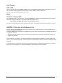
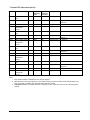
Meaning and Operation of Flags
The various bits in the FLAG value are as follows
Bit
0
1
2
3
4
5
6
7
8
9
10
11
12
11
14
15
Value
1
2
4
8
16
32
64
128
256
512
1024
2048
4096
8192
16384
32768
Description
(unused – reserved)
(unused – reserved)
Temperature under range ( TEMP)
Temperature over-range (TEMP
Strain gauge input under-range
Strain gauge input over-range
Cell under-range (CRAW)
Cell over-range (CRAW)
System under-range (SRAW)
System over-range (SRAW)
(unused – reserved)
Load Cell Integrity Error (LCINTEG)
Watchdog Reset
(unused – reserved)
Brown-Out Reset
Reboot warning (Normal Power up)
Name
Unused
Unused
TEMPUR
TEMPOR
ECOMUR
ECOMOR
CRAWUR
CRAWOR
SYSUR
SYSOR
Unused
LCINTEG
WDRST
Unused
BRWNOUT
REBOOT
NOTE:
The mnemonic names are used by convenience properties in Instrument Explorer, but are otherwise for reference
only –the flags can only be accessed via the FLAG parameter.
The various warning flags have the following meanings
TEMPUR and TEMPOR indicate temperature under-and over-range. The temperature minimum and maximum
settings are part of the temperature calibration, fixed at –50.0 and +90.0 ºC. Only active when optional
Temperature module fitted.
ECOMUR and ECOMOR are the basic electrical output range warnings. These are tripped when the electrical reading
goes outside fixed ±120% limits: This indicates a possible overload of the input circuitry, i.e. the input is too big to
measure.
The tested value, ECOM is an un-filtered precursor of ELEC
CRAWUR and CRAWOR are the cell output range warnings. These are tripped when the cell value goes outside
programmable limits CMIN or CMAX.
The tested value, CRAW is the cell output prior to linearity compensation.
SYSUR and SYSOR are the system output range warnings. These are triggered if the SYS value goes outside the SMIN
or SMAX limits.
LCINTEG indicates a missing or a problem with the Load cell. It is based on the common mode of the –SIG being
correct. NOTE This flag will also be set when the shunt calibration has been switched on.
WDRST indicates that the Watchdog has caused the device to re-boot. If this error continually occurs consult
factory.
Mantracourt Electronics Limited DCell & DSC CANopen® User Manual
26
BRWNOUT indicates that the device has re-booted due to the supply voltage falling below 4.1V, the minimum spec
for supply voltage is 5.6V and this must include any troughs in the AC element of this supply.
REBOOT is set whenever the DCell/DSC is powered up and is normal for a power up condition. This flag can be used
to warn of power loss to device.
Dynamic Status Flags (STAT)
Status are “live” flags, indicating current status of the device. Some of these flags have the same bit value &
description from “FLAG”.
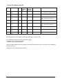
Meaning and Operation of Flags
The various bits in the STAT value are as follows
Bit
0
1
2
3
4
5
6
7
8
9
10
11
12
11
14
15
Value
1
2
4
8
16
32
64
128
256
512
1024
2048
4096
8192
16384
32768
Description
Setpoint output status
Digital Input status (DSC ONLY)
Temperature under range (TEMP)
Temperature over-range (TEMP
Strain gauge input under-range
Strain gauge input over-range
Cell under-range (CRAW)
Cell over-range (CRAW)
System under-range (SRAW)
System over-range (SRAW)
(unused – reserved)
Load Cell Integrity Error (LCINTEG)
Shunt Calibration Resistor ON
Stale output value (previously read)
(unused – reserved)
(unused – reserved)
Name
SPSTAT
IPSTAT
TEMPUR
TEMPOR
ECOMUR
ECOMOR
CRAWUR
CRAWOR
SYSUR
SYSOR
Unused
LCINTEG
SCALON
OLDVAL
Unused
Unused
SPSTAT indicates the state of the Open collector output, 1 being output on 0 being output off.
IPSTAT indicates the state of the digital input (Only available on DSC model). Bit set indicates input is ‘closed’ to
0v (-V or GND).
SCALON Used to indicate that the Shunt Calibration command, SCON, has been issued & therefore the shuntcal
resistor is now in circuit with the strain gauge bridge. SCOF command resets this bit. Note that when Shunt
Calibration is active the “Load Cell Integrity Error” will also be generated.
OLDVAL is set when the device is read via the communications. Thus indicating this value has already been
sampled. It is reset when a new result has been made available.
Output Update Tracking
The OLDVAL flag can be used for output update tracking
This allows sampling each result exactly once: To achieve this poll the STAT value until OLDVAL is cleared to
indicate a new output is ready, then read SYS, this reading will set the OLDVAL flag in STAT.
This scheme works as long as the communications speed is fast enough to keep up. With faster update rates and
slower baud rates, it may not be possible to read out the data fast enough.
27
Mantracourt Electronics Limited DCell & DSC CANopen® User Manual
User Storage
USR1…USR9
There are nine storage locations USR1 to USR9. These are floating point numbers which can be used for storage of
data. This data could be calibration time and date, operator number, customer number etc.
This data is not used in anyway by the DCell or DSC.
Reset
The Reset command, RST
This command is used to reset the device. This command MUST be issued if the following parameters are changed
before the change will take effect. Alternatively the power maybe cycled.
RATE, NODEIDL, NODEIDH, BPS and all of the Message parameters
The reset action may take up to about a second to take effect, followed by the normal start-up pause of 1 second.
WARNING: Finite Non-Volatile Memory Life
The DCell and DSC use EEPROM-type memory as the storage for non-volatile controls (i.e. all the settings that are
retained even when powered down).
The device EEPROM itself is specified for 100,000 write cycles (for any one storage location), although typically this
is 1,000,000. Therefore –
When automatic procedures may write to stored control parameters, it is important to make sure this does not
happen too frequently.
So you should not, for example, on a regular basis adjust an offset calibration parameter to zero the output value.
However, it is reasonable to use this if the zeroing process is initiated by the operator, and won’t normally be used
repeatedly.
For the same reason, automatically cancelling warning flags must also be implemented with caution: It is okay as
long as you are not getting an error recurring repeatedly, and resetting it every few seconds.
Mantracourt Electronics Limited DCell & DSC CANopen® User Manual
28
Chapter 4 The Readings Process
This chapter gives an account of the reading process except for the linearity-and temperature-compensation
processes (which have their own chapters later on).
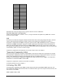
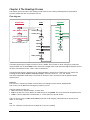
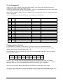
Flow diagram
Electrical
Cell
System
SGAI x
MMV
MMV/NMVV x 100%
ELEC
*OPTIONAL MODULE
* TEMP
*CTGx (Ctx) x
SOFS
*CTOx (Ctx)
SMIN
<
SRAWUR
SMAX
>
SRAWOR
CMVV
SRAW
CGAI X
SZ
COFS
CMIN
<
CRAWUR
SYS
CMAX
>
CRAWOR
SOUT
CRAW
CLKx (CLXx) +
CELL
The underlying analogue to digital conversion rate is 3.255Khz. These results are block averaged to produce the
required output rate set by the RATE control This block averaged result is then passed through the dynamic filter at
the same rate and then into the ‘chain’ of above calculations.
The named values shown in the boxes are all output parameters, which can be read back over the comms link.
The diagram shows three separate calibration stages, called the ‘Electrical’, ‘Cell’ and ‘System’.
This allows independent calibrations to be stored for the device itself, the load cell and the installed system
characteristics –
Electrical
The ‘Electrical’ calibration produces corrected electrical readings from the internal measurements.
This is factory-set by Mantracourt during the production process.
The main outputs from this are –
• MVV is the factory calibrated output, in mV/V units.
• ELEC is the mV/V in % terms. Where the 100% value is set using NMMV. This is for backwards compatibility only.
• TEMP is a device temperature measurement, in °C and requires an optional module.
There are also two flags, ECOMUR and ECOMOR (not shown on the diagram), which indicate an input electrical
under- or over-range.
Cell
The ‘Cell’ calibration converts the mV/V output into a cell-force reading.
29
Mantracourt Electronics Limited DCell & DSC CANopen® User Manual
This can be used by an OEM sensor manufacturer to provide a standard, calibrated output in force units, which could
be based on either typical or device-specific calibration data.
(This stage also includes the temperature- and linearity-corrections, not covered here)
The outputs from this are
• CMVV is the temperature compensated mV/V (MVV).
• CRAW is the scaled temperature compensated value CMVV
• CELL is a load cell force reading in “Force” units (e.g. kN)
• CRAWUR and CRAWOR are two flags indicating under or, over range for the force measurement.
System
The ‘System’ calibration converts the Cell output into a final output value, in the required engineering units.
This is normally be set up by a systems installer or end user, to provide whatever kind of output is needed,
independently of device-specific information in the Cell calibration.
(Making this split allows in-service replacement without re calibration).
The Outputs From This Are
• SRAW is a re-scaled and offset adjusted output derived from CELL
• SYS is the final output value, after removing a final user output offset value (SZ) from SRAW
• SRAWUR and SRAWOR are output warning limit flags.
In practice, SRAW and SYS can be used to represent something like gross and net values.
Cell and System Scaling
Both the Cell and System calibrations are simply linear rescaling calculations –i.e. they apply a gain and offset.
In both cases, four parameters define the scaling, offset and min and max limit values. These calculations are
applied in the following way:
Output = (Input × GAI) – OFS
Output = min (output, MAX)
Output = max (output, MIN)
(In addition, if the value exceeds either limit, one of two dedicated error flags is set)
The control parameters thus have the following characteristics: –
• GAI is the multiplying factor, set in “output-units per input-unit”
• OFS is the value that gives zero output, set in “output units”
• MAX and MIN are output limit values, set in “output units”
The units and functions of the main scaling controls can thus be summarised as –
Cell Calibration
CGAI
Force/mV/V
mV/V gain factor
COFS
Force
CELL Offset Value
CMIN
Force
Minimum value for CRAW
CMAX
Force
Maximum value for CRAW
System Calibration
SGAI
Eng/ Force
SOFS
Eng
SMIN
Eng
SMAX
Eng
SZ
Eng
SYS/CELL gain factor
SRAW value offset
Minimum value for SRAW
Maximum value for SRAW
SYS value offset
(MVV is mV/V, “force” is force units, and “eng” is engineering units)
Mantracourt Electronics Limited DCell & DSC CANopen® User Manual
30
Calibration Parameters Summary and Defaults
The various control parameters are listed for each stage.
This also includes the compensation parameters, not covered in this chapter, but shown in the flow diagram
The ‘default’ values shown set the device back to its nominal default calibration (mV/V)
Cell Control Defaults
Command
Action
FFLV
Filter dynamic level
FFST
Filter Steps (max)
NMMV
Nominal 2.5mV/V
RATE
Rate 10Hz
CGAI
basic cell gain
COFS
basic cell offset
CTN
number of temp points
CT1..5
temp points (Deg C)
CTO1..5
offset adjusts
CTG1..5
gain adjusts
CMIN
CRAW min limit
CMAX
CRAW max limit
CLN
number of linearity points
CLX1..7
linearity raw-value points
CLK1..7
linearity adjusts
Default Values
0.001
100
2.5
3
1.0
0.0
0
0.0, 0.0, 0,0…
0.0, 0.0, 0,0…
1.0, 1.0, 1.0, 1.0…
–3.0
+3.0
0
0.0, 0.0, 0,0…
0.0, 0.0, 0,0…
System Control Defaults
Command
Action
SGAI
basic gain
SOFS
basic offset
SMIN
SRAW min limit
SMAX
SRAW max limit
SZ
output zero offset
Default Values
1.0
0.0
–100.0
+100.0
0.0
31
Mantracourt Electronics Limited DCell & DSC CANopen® User Manual
Chapter 5 Temperature Compensation
This chapter explains how to use the Temperature Compensation facilities, to compensate for changes in the
measurement with ambient temperature.
Temperature compensation is only provided when an optional module consisting of a digital temperature sensor is
wired to the DCell or DSC.
Purpose and Method of Temperature Compensation
Most measurement methods are affected by changes in temperature, and (uncompensated) load cells are especially
sensitive, having a large overall temperature coefficient.
Temperature compensation adjusts the measured value in a way that depends on a temperature measurement, so
that (ideally) the output does not depend on the current temperature.
In practice, it is usual to refer to a calibration ‘reference’ temperature: The ideal output value is then what the
reading ‘would have been’ if made at the reference temperature.
The DCell/DSC temperature compensation facilities make adjustments to the ‘Cell’ calibration parameters (i.e. gain
and offset) which depend on temperature, according to a digitally programmed curve.
These adjustments are automatically applied, based on the current device temperature measurement. With some
care, this can remove the need for the usual electrical compensation components altogether.
Note that the temperature compensation will also remove the temperature drift of the DCell/DSC itself if the
temperature compensation data is collected when the DCell/DSC and strain gauges are tested together as a system.
Temperature Module Connections and Mounting (DTEMP)
The temperature module is a connected using only two wires. The temperature sensor is the Dallas “1-Wire” digital
device DS18S20. One connection is ground for which –EXC is used and the other is the 1 wire “DQ” connection which
provides the bi-directional data line.
+EXC
+SIG
-SIG
-EXC
Temp sensor “DQ”
Note: -EXC provides the ground connection to the optional temperature module.
For DSC the DQ connection is connected to the I/O pin marked TS.
The temperature module is a small double sided PCB with an 8 pin SOIC integrated circuit mounted to it. The
dimensions are 10.5 x 7.6 x 2.5mm. There are two solder pads for connection to the DSC or DCell. A 2mm hole is
used for fixing the temperature module to the body of the load cell. The module should, ideally, be positioned as
Mantracourt Electronics Limited DCell & DSC CANopen® User Manual
32
close as possible to the strain gauges. The IC on the temperature module must also be in good thermal contact to
the load cell body so the strain gauges and temperature sensor see the same temperature.
-EXC
DQ
Control Parameters
The temperature compensation parameters define a pair of lookup tables that contain adjustments to the cell
calibration gain and offset over temperature.
The parameters
CTN
CT1…CT5
CTO1…CTO5
CTG1…CTG5
concerned are
[-]
[°C]
mV/V
ppm
the following
Number of temperature table points
Indicated TEMP value at table point
MV/V (x104) Offset adjustment at Offset table point
Gain (x106) at Gain table point
CTN sets the number of points in the gain & offset table’s. A CTN value of less than two effectively switches off
temperature compensation. The maximum number of point is 5, values greater than 5 reset CTN to 0 switching off
temperature compensation.
CT1 to CT5 sets the temperature in degree C of the correction points. The table must be filled from CT1 up to &
including CT(CTN) and must be entered in order of increasing temperature value.
CTO1 to CTO5 provide the offset adjustment in mV/V x104. The reason for the multiplication is due to the
limitation set by the ASCII protocol of only being able to enter up to 6 decimal places. The CTOx value is subtracted
from the uncompensated value.
CTG1 to CTG5 provide the gain adjustment in ppm terms.
The actual gain value used is calculated as 1 + CTGn x 10-6 .
Internal Calculation
The temperature compensation calculation is described as follows:The GAIN correction is applied first. The current measured temperature is checked against the table values CT1 to
CT(CTN) to establish an index value if the measured temperature is below that of CT1 then CT1 is used as the index,
If the temperature is above CT(CTN-1) then CT(CTN-1) is used.
This can be represented as follows:A working table index, i, is derived from the current measured temperature, T, as follows —
(n = number of points used, as set by CTN)
When (T < CT1)
then i = 1
When (T > CTn-1)
then i = (n–1)
Otherwise
i is chosen so that Ti ≤ T ≤ Ti+1
Once an index into the table has been established the gain value to be used is extrapolated between the index value
and the value above. If the temperature is above CT(CTN) or below CT1 then the calculated temperature gain value
is extrapolated from CT(CTN-1) to CT(CTN) or CT1 to CT2 respectively.
This can be represented mathematically as follows:CALC_CTG = CTGi + (CTGi+1 – CTGi) × (T – CTi) / (CTi+1 – CTi)
The actual gain value used is 1 + CALC_CTGO x 10-6 and is multiplied by the uncompensated value MVV.
The offset correction is then applied. Using the same temperature index “i” as found for the GAIN index above.
33
Mantracourt Electronics Limited DCell & DSC CANopen® User Manual
The Offset value is extrapolated between the same two temperature points.
This can be represented mathematically as follows:CALC_CTO = CTOi + (CTOi+1 – CTOi) × (T – CTi) / (CTi+1 – CTi)
The actual offset value used is CALC_CTO x 10-4 and is subtracted from the above gain adjusted value.
The output from the temperature compensation (CMVV) is then calculated as
CMVV = MVV x (1 + CALC_CTGO x 10-6) - (CALC_CTO x 10-4)
The Temperature Measurement
The temperature sensor used is a Dallas (MAXIM) DS18S20 Digital Thermometer using the “1-Wire” bus technology.
This gives a temperature measurement accuracy of +/-0.5 Degree C over the temperature range –10 to +85 degree C
and +/-2.0 Degree C over temp range –55 to +125 Degree C. The resolution of the measurement is 0.0625 Degree C.
The temperature is sampled and the TEMP variable updated every 5 seconds.
How to Set Up a Temperature Compensation
There are a number of ways of obtaining a temperature compensation curve.
The best possible compensation for a given piece of physical hardware can only be achieved by performing
experiments on that particular unit (DCell/DSC and associated strain gauges), to characterise the measurement
output at a variety of different, stable temperatures in the required operating range.
The basic choice of methods depends on trading off ideal accuracy against the complexity of the calibration
procedure.
Method 1
Apply a simple linear drift correction (i.e. for known constant gain and offset changes per degree), by specifying
zero correction at the calibration temperature, and appropriately adjusted correction values at extreme
temperatures above and below this.
This can be used when the measurement or sensor has known temperature coefficients.
Method 2
Where the temperature characteristics of the measurement are known, but not linear, a similar scheme to Method 1
can be used, with a multi-point table defining an approximation to the known, ideal temperature curves of offset
and gain variations.
NOTE: Both of the above methods are based on ‘known’ characteristics, which could come from datasheets but
these methods would not compensate for the DCell/DSC.
Method 3
Do a series of measurements at different temperatures and install the appropriate correction values to give exactly
correct results at those same temperatures –i.e. calculate ideal gain and offset corrections at the tested
temperatures.
(This method is the most common). There is a ‘wizard’ available in Instrument Explorer which will enable this
method to be easily completed by calculating the gain and offset corrections for you.
Method 4
Use a set of test results to plan a ‘best correction’ curve (not necessarily perfect at test temperatures, but slightly
better overall).
NOTES:
All of these methods can be applied either to data from individual devices or to an ‘average’ correction for a
particular type of sensor hardware.
During testing, temperatures should be measured using the internal TEMP measurement, as this is the measurement
used to do the corrections.
For in-system tests, the environment of the DCell/DSC must always be as near as possible to the exact conditions of
the eventual in-system use.
Mantracourt Electronics Limited DCell & DSC CANopen® User Manual
34
Parameter Calculations
Instrument Explorer provides a “Wizard” for the calculation of the parameters required by the DSC/DCell. This is
based on Method 3 where data is collected. The wizard allows for small changes in the sampled temperature point
that may occur when taking a set of results for gain and offset. Also taken into account is any variation in the test
weights at different temperatures. This is a complex mathematical procedure which is best solved by a PC
programme such as the wizard.
35
Mantracourt Electronics Limited DCell & DSC CANopen® User Manual
Chapter 6 Linearity Compensation
This chapter describes the Linearity Compensation features and how to use them.
Purpose and Method of Linearisation
Load cell sensor outputs are never precisely proportional to the input (applied load).
If the graph of the measurement output against the true value shows slight deviations from the ideal straight-line,
then slight errors remain even when the basic calibration (offset and gain) is as good as possible.
Linearity compensation adjusts the raw measurement by a small amount that is calculated as a function of the raw
measurement value itself. Ideally this will adjust the output response, for any given input load, by exactly the right
amount to place the final result onto the ideal straight line.
The DCell/DSC non-linearity compensation uses a single ‘lookup table’, similar to those used for temperature
compensation (see previous chapter). This provides a linearly-interpolated compensating value with up to 7 control
points, which is then added to the output result.
Generally, linearisation is a finer level of compensation than temperature compensation.
It should only be applied after the basic Cell calibration and temperature compensation (if any) have been set up.
Although the tests are generally simpler than testing over temperature, the accuracy requirement is often greater.
See below for notes of possible difficulties to be avoided.
Control Parameters
Refer to the table in Chapter 9 for command numbers
The lookup table (based on parameters CLXi, CLKi) defines an offset adjustment based on the CRAW value, which is
then added in to give the final CELL output.
(So linearity correction is applied after any temperature compensation.)
The Parameters Involved Are :
CLN
Sets the number of linearisation points (from 2 up to 7)
CLX1..7
Raw input (CRAW) value points
CLK1..7
Output (CELL) adjustments to apply at these points
They are used like this :
• The number of calibration points is set by CLN (from 2 up to 7)
• Raw input value points are set by CLX1, CLX2 .. CLX7 (or up to the number set by CLN)
These must be arranged in order of increasing input value.
• The output corrections at these points are set by CLK1, CLK2 .. CLK7
• Corrections are specified in “thousandths of a cell unit”. So a CLKi of 1.0 actually adds 0.001 to the CELL
output). This due to a limitation in the ASCII conversion to floating point numbers.
Internal Calculation
This uses the same basic ‘interpolated table lookup’ method as for temperature compensation.
First, a working table index, i, is derived from the current raw input CRAW=x, as follows :
(n = number of points used, as set by CLN)
When (x < CLX1)
then i = 1
When (x > CLXn-1)
then i = (n–1)
Otherwise
i is chosen so that CLXi ≤ x ≤ CLXi+1
The resulting interpolated adjustment value is then calculated as –
ofs = CLKi + (CLKi+1 – CLKi) × (x – CLXi) / (CLXi+1 – CLXi)
Then the compensated cell value is calculated as –
CELL = CRAW + ofs
Mantracourt Electronics Limited DCell & DSC CANopen® User Manual
36
How to Set Up Linearity Compensation
A linearity correction can be set up either from sensor specification/calibration data, or more commonly from insystem testing results.
Assuming we do not have any prior information on linearity errors, the usual approach is to do a series of controlled
tests with accurately known test loads.
Just as with temperature compensation, it is possible to obtain a detailed graph of linearity error and then choose a
‘best-fit’ piecewise linear curve for the compensation table.
However, it is generally good enough, and much simpler, to simply test at several different points and then apply an
exact correction at those points. If the error curve is reasonably smooth, this should give exact results at the test
points, and reasonably accurate values in between.
NOTES:
Linearisation tests should only be done after the cell calibration is set, because the correction values are dependent
on the cell calibration.
Similarly, linearisation testing should only be done at the calibration ‘reference’ temperature, or after temperature
compensation is installed, to avoid temperature effects from distorting the results.
The linearisation tests should not reveal any significant remaining linear trend in the errors.
If errors do appear to lie on a definite line, this could drastically reduce the accuracy of the correction.
If this does happen, it shows that the cell calibration is wrong and should be redone.
The table points must always cover more-or-less the whole range of output values to be used, because corrections
are extrapolated outward beyond the first and last points.
It is always worthwhile including more test-points than will be used in the correction table, because this gives
confidence that no regions of rapidly changing error have been missed.
Tests should be done both with steadily increasing and decreasing load values, as hysteresis effects (for load cells)
are often of a similar size to non-linearities.
Parameter Calculations and Example
Based on the simple method outlined above, we suppose that we have obtained test results for a series of precisely
known load values –
test loads Xi give readings of CRAW = Ci, for (i = 1..n)
Then calculate the errors that need to be removed at these points –
Ei = Xi – Ci
Now just enter these values into the correction table, remembering to scale the errors –
CLN = n
CLXi = Xi
CLKi = 1000 • Ei
Example
Suppose we have a load cell and Cell calibration giving a result in the range 0-500 KgF.
The following test results were obtained using a series of known test loads –
For test load of x1 = 0Kg
:
CELL reading c1 = 0.0010
For test load of x2 = 100.13Kg :
CELL reading c2 = 100.44
For test load of x3 = 199.72Kg :
CELL reading c3 = 200.57
For test load of x4 = 349.97Kg :
CELL reading c4 = 349.75
For test load of x5 = 450.03Kg :
CELL reading c5 = 449.98
We choose these precise test points as our linearisation reference points, so
CLN = 5
CLX1 = 0.0010
CLX2 = 100.44
37
Mantracourt Electronics Limited DCell & DSC CANopen® User Manual
CLX3 = 200.57
CLX4 = 349.75
CLX5 = 449.98
(Note that these are the raw reading values, not the known true values.)
Now calculate all the residual errors, and set up the correction factors –
CLK1 = 103×(x1 – c1) ≈ 1000×
×(000.00–0.0010) = –1.0
CLK2 = 103×(x2 – c2) ≈ 1000×
×(100.13–100.44) = –310.0
CLK3 = 103×(x3 – c3) ≈ 1000×
×(199.72–200.57) = –850.0
CLK4 = 103×(x4 – c4) ≈ 1000×
×(349.97–349.75) = +220.0
CLK5 = 103×(x5 – c5) ≈ 1000×
×(450.03–449.98) = +320.0
The CELL output values will now have the required values at all these 5 points.
Note on the Example
If you graph the errors from the above example, the results look like this
0.4
0.2
0
-0.2
0
100
200
300
400
500
-0.4
-0.6
-0.8
-1
This doesn’t show any very definite linear trend, so the calibration is okay.
However there is a big jump between points 3 and 4, which might be worth a more detailed investigation: Some
important features of the error curve could have been missed by the test.
Mantracourt Electronics Limited DCell & DSC CANopen® User Manual
38
Chapter 7 Self-Diagnostics
Diagnostics Flags
The main diagnostics facilities are by means of the flags. See chapter 3 Flags for a full description of the flags and
their meaning.
The flags are normally used something like this.
FLAG is read at regular intervals by the host (like the main output value, but generally at longer intervals)
If some warnings are active, i.e. FLAG is non-zero, then the host tries to cancel the warnings found by writing
FLAG= 0
The host then notes whether the error then either remains (i.e. couldn’t be cancelled), or if it disappears, or if it
re-occurs within a short time, and will take action accordingly.
The warning flags are latched indicators of transient error events: By resetting the register, the host both signals
that it has seen the warning, and readies the system to detect any re-occurrence (i.e. it resets the latch).
What the host should actually do with warnings depends on the type and the application: Sometimes a complete log
is kept, sometimes no checking at all is needed.
Often, some warnings can be ignored unless they recur within a short time.
Warning flags survive power-down, i.e. they are backed up in non-volatile (EEPROM) storage.
Though useful, this means that repeatedly cancelling errors which then shortly recur can wear out the device nonvolatile storage – see WARNING: Finite Non-Volatile Memory Life in chapter 3.
STAT provides a current status of the device. These flags are not latched and not saved on power fail.
Diagnostics LED
A new feature for Version 3 is the addition of an LED to indicate the current status of the device. If all is healthy the
LED should flash ON for a period of 100mS , The rate at which the LED flashes is 0.5 second.
If an error conditions occurs which is based on any of the following error flags being set then the operation
of the LED will invert. IE the LED will flash off for 100mS at the rate set in the table above.
These flags Being, TEMPUR, TEMPOR, ECOMUR, ECOMOR, CRAWUR, CRAWOR, SYSUR, SYSOR & LCINTEG.
39
Mantracourt Electronics Limited DCell & DSC CANopen® User Manual
Chapter 8 CANopen® Communication Protocol
This chapter gives details of communication protocols and bus connections.
This manual only covers CANopen® communications.
The user will need a suitable CANopen® bus-master application to communicate with DSC.
(Details of suitable solutions are available from Mantracourt on request).
CANopen® Features Support Summary
Device Profile
NMT support
Boot up
COB ID Distribution
Node ID Distribution
PDO’s
SDO’s
PDO modes
Variable PDO mapping
Emergency Message
Life Guarding
Heartbeat Producer
Manufacturer defined (type 0)
Slave device
Minimum boot up device
by SDO (no DBT support)
by SDO (no LMT support)
4tx, 0rx
1
Sync, Async, Cyclic, Acyclic
Y Maximum 2 objects / PDO
Y
N
Y
Additional Notes:
Changes to NodeID, CANbus Bit Rate and PDO communication Parameters will require the device to be power cycled.
Mantracourt Electronics Limited DCell & DSC CANopen® User Manual
40
Object Dictionary Summary
DSC & DCELL internal data values are mapped into the object dictionary in three distinct areas :–
1. The main output values are mapped into the ‘Device Profile’ area, at 6000h onward
2. Special control parameters, specific to the CANopen® version, are at 2000h onward
3. The DCell, DSC internal Configuration parameters are mapped at 5000h onward
Object
index
Subindex
Type
Description
Access
[Default]
1000
–1FFF
–
–
–
Standard communications area
–
2000
2001
0
0
UNSIGNED8
UNSIGNED8
R/W
R/W
CANopen® node id
CANbus bitrate control
127 (0x7F)
3 = 125kb/s
5000
–5FFF
0
SIGNED32
–
DSC internal parameters
–
6000
6001
0
0
FLOAT32
UNSIGNED16
RO
RO
–
–
6002
0
FLOAT32
RO
“SYS” main value output (Scaled)
DSC “FLAG” error register
“SYSN” main value (Snapped SYS
Value)
–
The device supports a manufacturer-specific device profile with Limited PDO mapping of 2 objects to each
Transmit PDO. The following communications objects are implemented:–
•
•
•
•
•
41
SDO
Transmit
Transmit
Transmit
Transmit
PDO-1
PDO-2
PDO-3
PDO-4
Mantracourt Electronics Limited DCell & DSC CANopen® User Manual
Error Management
The DSC “FLAG” value is mapped to the profile object at 6001h. Flags set also cause appropriate bits in the
standard Error Register (object index 1001h) to be set.
In some cases, an Emergency telegram is also broadcast. In this case, the “Manufacturer Specific Error Field” simply
contains the actual 16-bit “FLAG” value, followed by void bytes.
When the error condition is removed, the error register reverts to 0, and a further “NO error” emergency telegram
is sent, if appropriate.
The error and emergency codes generated by DSC error conditions are the following :—
Bit
Value
Description
0
1
2
3
4
5
6
7
8
9
10
11
12
11
14
15
1
2
4
8
16
32
64
128
256
512
1024
2048
4096
8192
16384
32768
(unused – reserved)
(unused – reserved)
Temperature under range ( TEMP)
Temperature over-range (TEMP
Strain gauge input under-range
Strain gauge input over-range
Cell under-range (CRAW)
Cell over-range (CRAW)
System under-range (SRAW)
System over-range (SRAW)
(unused – reserved)
Load Cell Integrity Error (LCINTEG)
Watchdog Reset
(unused – reserved)
Brown-Out Reset
Reboot warning (Normal Power up)
Error Register
Bit(s)
Unused
Unused
0,3 = temp
0,3 = temp
0,7 = mfr-specd
0,7 = mfr-specd
0,7 = mfr-specd
0,7 = mfr-specd
0,7 = mfr-specd
0,7 = mfr-specd
0,7 = mfr-specd
0,7 = mfr-specd
0,7 = mfr-specd
0,7 = mfr-specd
0,7 = mfr-specd
0,7 = mfr-specd
Emergency Telegram Code
NONE
NONE
4200h = device temp
4200h = device temp
6000h = device software
Communications Controls
The units NODE ID is configured over the CAN BUS by writing to the object at index 2000h sub index 0.
The Node ID is stored in non volatile memory and changes will not take effect until the unit is power cycled.
Units are delivered with a CANopen® Node-ID set to 127
The CANbus Bit Rate can be configured by writing to the object at index 2001h sub index 0, where the following
value settings are defined :–
Setting:
Rate/kbs
0
20
1
50
2
3
4
5
6
100
125
250
500
800
7
1000
If a value < 0 or > 7 is sent to the unit the next time the power is cycled the unit will return to it’s default
Bit rate of 125 Kbits to avoid loosing communications with the unit by entering an invalid Bit Rate. It is Essential
that the Bit Rate is set correctly or communications with the device will no longer be possible.
Again stored in non volatile memory and changes will not take effect until the unit is power cycled.
On receiving a NMT “Reset_Node” or “Reset_Communication” service, all the device-independent communications
settings revert to the CANopen® standard default settings. The Node-ID and Bit Rate are not reset by this.
Mantracourt Electronics Limited DCell & DSC CANopen® User Manual
42
Data Type Conversions and Rounding
Type Conversion
Depending on the protocol, an integer/byte parameter may need to be converted to or from a floating-point
representation for reading or writing.
The rules are as follows
For reading, integer and byte parameters are treated as unsigned, and never read negative
– i.e. read value ranges are 0 to 65535.0 and 0 to 255.0
For writing, values written to integer and byte parameters are truncated to the nearest integer, and negative or
positive values are acceptable
NOTE: Floating-point data is not always exact, even when reading integral data
e.g. could get 3.999974 instead of 4
e.g. for a byte write 240, 240.1 and 239.66 are all the same value
Rounding
Although rounding is applied when writing to integral values, data read from a device is not rounded off.
43
Mantracourt Electronics Limited DCell & DSC CANopen® User Manual
Chapter 9 Object Dictionary
This chapter contains tables of all DCell/DSC Object Dictionary, with brief details of each.
Communications Profile Area
Device Description and Communication Specific
Name
Description
Access
-
DEVICE TYPE
ERROR REGISTER
PRE-DEFINED ERROR FIELD
COB-ID SYNC MESSAGE
RESTORE ALL PARAMETERS FROM 1000H TO
2001H
RESTORE COMMUNICATIONS PROFILE
PARAMETERS 1000H TO 1FFFH
RESTORE CAN COMMUNICATIONS
NODE ID & BITRATE
-
RO
RO
RO
RO
WO
Object
Dictionary
Index
1000h
1001h
1003h
1005h
1011h
Object
Dictionary
Sub Index
0
0
0
0
1
WO
1011h
2
WO
1011h
4
Data Type
Unsigned 32 bit
Unsigned 8 bit
Unsigned 32 bit
Unsigned 32 bit
Unsigned 32 bit
note 1
Unsigned 32 bit
note 1
Unsigned 32 bit
note 1
Note 1 should always be 4 bytes value = “SAVE”
MSB
65h
‘e’
76h
‘v’
61h
Mantracourt Electronics Limited DCell & DSC CANopen® User Manual
‘a’
LSB
73h
‘s’
44
Transmit PDO Operation Specific
Name
Description
PDOT1
TPDO 1 transmit
Type
TPDO 1 COBID
PDOC1
PDOI1
PDOE1
PDOT2
PDOC2
PDOI2
PDOE2
PDOT3
PDOC3
PDOI3
PDOE3
PDOT4
PDOC4
PDOI4
PDOE4
Access Object
Dictionary
Index
RW
1800h
Object
Data Type
Dictionary
Sub Index
02h
Unsigned 8 bit
RW
1800h
01h
RW
RW
1800h
1800h
03h
05h
Unsigned 32 bit 0 = Use default of 0x180 + Node ID
See Note 3
Unsigned 16 bit 0 = Disabled
Unsigned 16 bit 100mS
RW
1801h
02h
Unsigned 8 bit
RW
1801h
01h
RW
RW
1801h
1801h
03h
05h
Unsigned 32 bit 0 = Use default of 0x280 + Node ID
See Note 3
Unsigned 16 bit 0 = Disabled
Unsigned 16 bit 100mS
RW
1802h
02h
Unsigned 8 bit
RW
1802h
01h
RW
RW
1802h
1802h
03h
05h
Unsigned 32 bit 0 = Use default of 0x380 + Node ID
See Note 3
Unsigned 16 bit 0 = Disabled
Unsigned 16 bit 100mS
RW
1803h
02h
Unsigned 8 bit
RW
1803h
01h
TPDO 4 Inhibit timer RW
TPDO 4
RW
Transmission
interval
1803h
1803h
03h
05h
Unsigned 32 bit 0x80000000 = Disabled
See Note 3
Unsigned 16 bit 0 = Disabled
Unsigned 16 bit 100mS
TPDO 1 Inhibit timer
TPDO 1
Transmission
interval
TPDO 2 transmit
Type
TPDO 2 COBID
TPDO 2 Inhibit timer
TPDO 2
Transmission
interval
TPDO 3 transmit
Type
TPDO 3 COBID
TPDO 3 Inhibit timer
TPDO 3
Transmission
interval
TPDO 4 transmit
Type
TPDO 4 COBID
Default
255 = Use Event timer
255 = Use Event timer
255 = Use Event timer
255 = Use Event timer
Note
1. Each TPDO can have a maximum of two objects mapped.
2. PDO Parameters are stored directly to non volatile memory but will not take effect until the device has
been re-booted or an NMT reset communications has been issued.
3. 0x80000000 disables the TxPDO otherwise, setting a non zero value will result in this value being used
instead.
45
Mantracourt Electronics Limited DCell & DSC CANopen® User Manual
Transmit PDO Mapping Specific
Name
Description
PDOP1
TPDO 1 Mapping
item 1
TPDO 1 Mapping
item 2
TPDO 2 Mapping
item 1
PDOS1
PDOP2
PDOS2
PDOP3
PDOS3
PDOP4
PDOS4
Access Object
Dictionary
Index
RW
1A00h
RW
1A00h
Object
Data Type
Defaults
Dictionary
Sub Index
01h
See details below 0x50050004
‘SYS’, Sub Index 0, Length of 4 Bytes
02h
See details below 0 = Disabled
RW
1A01h
01h
TPDO 2 Mapping
item 2
TPDO 3 Mapping
item 1
RW
1A01h
02h
RW
1A02h
01h
TPDO 3 Mapping
item 2
TPDO 4 Mapping
item 1
TPDO 4 Mapping
item 2
RW
1A02h
02h
See details below 0x500D0002
‘SYSN’, Sub Index 0, Length of 4
Bytes
See details below 0 = Disabled
RW
1A03h
01h
See details below 0 = Disabled
RW
1A03h
02h
See details below 0 = Disabled
See details below 0x50090002
‘FLAG’, Sub Index 0, Length of 2
Bytes
See details below 0 = Disabled
PDO mapping data entries consist of the following data, which are 4 bytes total
First Two bytes are Object dictionary index to be mapped
Third byte is object dictionary sub index
Forth byte is the required data length
Note: The TxPDOs defaults have been mapped to the Manufacturers Specific Profile Area and not the Standardised
Device Profile Area.
Name refers to the Instrument Explorer Name.
Mantracourt Electronics Limited DCell & DSC CANopen® User Manual
46
Manufacturer Specific Area
Name
Description
CMVV
STAT
MVV
SOUT
SYS
TEMP
SRAW
CELL
FLAG
CRAW
ELEC
SZ
SYSN
PEAK
TROF
SERL
SERH
RATE
NMVV
CGAI
COFS
CMIN
CMAX
CLN
CLX1..7
CLK1..7
SGAI
SOFS
SMIN
SMAX
USR1..9
FFLV
FFST
CTN
Temp Compensated mV/V
Status
Filtered & factory calibrated mV/V
Selected output (copy of SYS)
Main output
Temperature
Raw System output
Cell output
Error flags
Raw cell output
Electrical output
System zero
Snapshot result
Peak value
Trough value
Serial number low
Serial number high
Reading rate select
Nominal mV/V for scaling ELEC
Cell gain
Cell offset
Cell range min
Cell range max
Number of Linearisation points
Linearisation raw-values
Linearisation corrections
System gain
System offset
System range min
System range max
User storage values
Dynamic Filter Level
Dynamic filter steps
Number of Temperature Compensation
points
Temperature Compensation Point
Temperature Compensation Gain adjust
Temperature Compensation Offset Adjust
Reset
Take snapshot
Reset peak & trough
Shunt cal ON
Shunt cal OFF
Digital Output On
Digital Output Off
CT1..5
CTG1..5
CTO1..5
RST
SNAP
RSPT
SCON
SCOF
OPON
OPOFF
Access Object Dictionary
Index
RO
5000h
RO
5001h
RO
5002h
RO
5003h
RO
5005h and 6000h
RO
5006h
RO
5007h
RO
5008h
RW
5009h and 6001h
RO
500Ah
RO
500Bh
RW
500Ch
RO
500Dh and 6002h
RO
500Eh
RO
500Fh
RO
5010h
RO
5011h
RW
5014h
RW
5015h
RW
5016h
RW
5017h
RW
5018h
RW
5019h
RW
501Eh
RW
501Fh .. 5025h
RW
5026h .. 502Ch
RW
502Dh
RW
502Eh
RW
502Fh
RW
5030h
RW
5031h .. 5039h
RW
503Ch
RW
503Dh
RW
503Eh
Object Dictionary
Sub Index
0
0
0
0
0
0
0
0
0
0
0
0
0
0
0
0
0
0
0
0
0
0
0
0
0 .. 0
0 .. 0
0
0
0
0
0 .. 0
0
0
0
RW
RW
RW
WO
WO
WO
WO
WO
WO
WO
0 .. 0
0 .. 0
0 .. 0
0
0
0
0
0
0
0
503Fh .. 5043h
5044h .. 5048h
5049h .. 504Dh
5050h
5051h
5052h
5053h
5054h
5050h
5051h
Table Key
“..” - Denotes a range (e.g. CLK1..7 means “CLK1” to “CLK7”)
Access RW/RO/WO/X = read-write / read-only / write-only / execute
47
Mantracourt Electronics Limited DCell & DSC CANopen® User Manual
Chapter 10 Installation
This chapter gives detailed information on integrating DCell and DSC devices into a production system – including
mounting, protection, adjustments, wiring and electrical requirements.
Before Installation
Carefully remove the DCell/DSC device from its shipment box. Check that the device is complete and undamaged.
Check the Product Type Code – on the product label is that which you ordered.
The DCell/DSC can operate in any industrial environment providing the following limits are not exceeded
Operating Temperature
Humidity
Storage temperature
-40 ºC to +85 ºC
95% non condensing
-40 ºC to +85 ºC
For precise details of Environmental Approvals, see chapter 15.
It
•
•
•
•
Is Advisable To Follow The Following Installation Practice Where Possible
Minimise vibration
Do not mount next to strong electrical or magnetic fields (transformers, power cables)
Install electrical protection device as the unit is not internally fused
Always ensure the package is secure and protected
Physical Mounting
DCell is normally sealed in the pocket of the load cell, which provides mechanical and moisture protection, and
electrical shielding.
The DCell should be mounted using a 2mm screw to the body of the load cell. This should be a “Good”
electrical connection to obtain maximum performance.
Connecting wires are soldered directly to the pads on the top and/or bottom of the PCB. Care must be taken to
electrically insulate the connection pads from the surrounding metal.
DSC is normally installed in a protective enclosure, such as a metal box.
The pins can be plugged into standard (0.1” pitch) PCB header sockets, or soldered directly into a host board or to
connecting wires.
It can be mounted either way up. Unwanted pins projecting on one side may be cropped off.
For extra vibration resistance, the 3 mounting holes provided can be used.
If not required, the protruding end with the single hole can be cut off to make the board smaller.
Electrical Protection
No additional electrical shielding is normally needed.
Electrostatic protection is sufficient for installation purposes only.
Devices are protected against shorting of communications lines to power supply, and shorting of sensor inputs.
No over-current protection is provided in case of faults, so the supply arrangements should ensure adequate power
limiting or fusing.
NOT PROTECTED AGAINST REVERSE POLARITY OF SUPPLY.
Moisture Protection
Both DCell and DSC must only be operated in a dry environment, as moisture can dramatically degrade the
measurement performance.
DCell
Will normally be sealed into a load cell pocket.
While flexible silicone sealant can be used to completely embed the unit, this is not adequate moisture protection
in itself.
If required, the entire unit can be embedded in a potting compound: A two-part epoxy compound can be used, but
bubbles and gaps must be avoided to prevent mechanical stress which could break the device.
Mantracourt Electronics Limited DCell & DSC CANopen® User Manual
48
The compound used must be specified for electrical use, and have sufficient thermal conductivity to cope with the
heat given off (up to 1W on a 15V supply).
DSC no additional electrical shielding is required, but moisture and/or mechanical protection are often required.
Any simple box or enclosure can be used. If metal, the enclosure should be grounded to the SH connection (see
Communications Cabling and Grounding Requirements below).
Soldering Methods
Take care soldering cables to the pads. Use a temperature controlled soldering iron set to a maximum 330ºC, for no
longer than 2 seconds per pad. Excessive heat or increased soldering time may result in damage to the PCB.
NOTES:
1. Solder with water-soluble flux should not be used (even low-residue), as this can leave a surface film which
attracts atmospheric moisture, degrading measurement performance.
2. DCell units can be damaged by poor soldering, due to the small nature of the circuit boards: Overheating or
applying any pressure to a pad can de solder components on the other side of the board, or cause the pad itself
to become detached.
Power Supply Requirements
The power supply needed is nominally 5.6 to 18V DC, but any possible droop or ripple must be included: The
devices contain ‘brown-out’ detection, which may trigger if the supply voltage at the device drops below the 5.6
volts.
A single device consumes typically 40mA with a 350Ω gauge connected (except RS232-output units, which use about
10mA more).
An installation should therefore assume at least 60mA per unit, and allow for extra current being taken at power-on
(though supply voltage can safely drop temporarily), and for possible voltage drops in long cables.
Any power-supply ripple should be below 100mV, and supply arrangements should provide current limiting for fault
conditions (see Electrical Protection, above).
Cable Requirements
Strain Gauge input (DSC)
For optimal performance twin twisted pair with individual shields is recommended, this gives good noise immunity.
Maximum length should not exceed 20m. Normal 4 core shielded cable can be used in areas of low electromagnetic
noise.
Power and Communication
Again, twin twisted pair cable is recommended for this. The cable should have the following characteristics.
• Twisted-pair with independent shields
• Characteristic impedance 50-150 ohms.
• Core to core and core to shield capacitance below 300pF/m
A suitable type is BICC Brand-Rex BE56723 (also equivalent to Belden type 8723).
In the UK, this is available from Farnell, part number 118-2117
Temperature Sensor
A shielded twisted pair is recommended, with a maximum length of 10m the shield being connected to the load cell
body or (CH if DSC). For short lengths (< 2m) in a low noise environment (inside load cell body for example) then
normal cable can be used.
49
Mantracourt Electronics Limited DCell & DSC CANopen® User Manual
Identifying Strain Gauge Connections
DCell Input Connections
+EXC
+SIG
-SIG
-EXC
Temp sensor “DQ”
The Optional Temperature sensor has two connections, “DQ” which provides the bi-directional data line and –EXC
which provides the 0v connection.
DSC Input Connections
Strain Gauge Bridge Connections Are As Follows
• EXC+/– positive/negative excitation (supply)
• SIG+/– positive/negative output signal
• SH Shield connection for shield of strain gauge cable
• GND can be used as the ground connection for the temperature sensor
Other Connections (DSC ONLY)
Resistor RG and track-cut TC are used to adjust the mV/V sensitivity (see Strain Gauge Sensitivity Adjustment,
below).
Identifying Bus-End Connections
DCell Bus Connections
CANL
CANH
+V
-V
Mantracourt Electronics Limited DCell & DSC CANopen® User Manual
50
DSC CAN Versions-Bus Connections
+V and -V are the DC power-supply and return connections
CANH & CANL are the CAN communications connections
GND is a communications ground connection
SH is the shield ground, used for shielding and grounding only
OP is the open collector digital output
IP is the volt free digital input
TS connects to DQ of the optional temperature sensor
•
•
•
•
•
•
•
Strain Gauge Cabling and Grounding Requirements
To achieve full performance specifications and conform to environmental approvals, it is important to follow
the wiring procedures outlined in this section.
DCell Strain Gauge Wiring
The following diagram illustrates how to wire up a DCell to a strain gauge
DCell Strain Gauge Wiring Arrangement
+ Exc
- Sig
STRAIN
GAUGE
+ Sig
Load Cell Body
- Exc
M2 Screw to Metal Body
Load Cell Body is Grounded
Key Requirements
All the load cell wires should be kept as short as feasible, at most 20cm.
The EXC+/– wires should be twisted together, also the SIG+/– pair, and the two pairs kept apart. It is also
recommended to secure the wires from moving due to shock or vibration. If the DCell is mounted outside the body
of the load cell then, for optimal performance, twin twisted cable should be used, although standard 4 core shield
cable can be used in low noise environments.
The M2 mounting hole must be grounded via an M2 screw to the load cell body for specified performance to be
met. (The 2mm mounting hole to accept M2 screw or American equivalent #0-80. Important Note: DO NOT USE #2
screw size.)
51
Mantracourt Electronics Limited DCell & DSC CANopen® User Manual
DSC Strain Gauge Cabling Arrangement
*Shield
EMC Gland
STRAIN
GAUGE
Note shield terminated
at EMC gland using
360° termination
*Tail length must be kept
to a mimimum
Key Requirements
The Strain Gauge cable should be a twin twisted pair with independent shields, with the two pairs used for the EXC
and SIG signal-pairs.
For specified performance, the load cell must be grounded to the SH.
DSC Sensor Cable
require 2 × twisted-pair version, otherwise similar to the above.
A suitable type is BICC Brand-Rex PD3003 (also equivalent to Belden type 8777).
In the UK, this is available from Farnell (enter ‘Belden 8777’ for real length options).
Mantracourt Electronics Limited DCell & DSC CANopen® User Manual
52
Communications Cabling and Grounding Requirements
To achieve full performance specifications and conform to environmental approvals, it is important to follow
the wiring procedures outlined in this section.
DCell Power and Communications Wiring
The following diagram illustrates how to connect a puck to the communications and power supply (“bus”) cable.
DCell Bus-End Arrangement
Note: The
specified cable
above shows a
yellow wire this
will be replaced
with a white wire.
EMC Gland
M2 screw to metal body
2 x Twisted Pair
CANH
CANL
+
-
Note shield terminated
at EMC gland using
360° termination
CANGND
+
PSU
Body is Grounded
Key Requirements
The cable must enter the load cell via an EMC cable gland, which connects the cable shield to the load cell body.
This must be a 360 Degree connection
The cable should be a twin twisted pair with independent shields, with one pair used for the communications and
the other for the power wires.
There MUST be a common connection from the PSU and the CAN ground to ensure the CAN stays within the required
common mode voltage of -2v (CANL) to +7v (CANH).
The shield should be connected to the grounded enclosure of the power supply.
53
Mantracourt Electronics Limited DCell & DSC CANopen® User Manual
DSC4 Versions- Power and Communications Wiring
The following diagram illustrates how to connect a DSC4 card to the communications and power supply (“bus”)
cable.
DSC4 Versions-Bus-End Arrangement
CANH
CANL
+
-
CANGND
+
PSU
Note: The specified cable above shows a yellow wire this will be replaced with a white wire.
Key Requirements
The cable should be a twin twisted pair with independent shields, with one pair used for the communications and
the other for the power wires.
The cable shield must be grounded to the SH pin at the DSC end, and not at the host end.
Any further metal housing should also be grounded to the DSC pin, and should not be connected to the bus cable
shield (or the sensor cable).
There MUST be a common connection from the PSU and the CAN ground to ensure the CAN stays within the required
common mode voltage of -2v (CANL) to +7v (CANH).
Suitable Cable Types
DCell/DSC CAN Bus Cable
The Cable requirements are dependent on the bit rate of the CAN bus and the required distances. Special care is
required for bit rates of over 500Kbps not only in the choice of cable used but how the bus wiring is organised ie the
requirement for very small stub lengths for high bit rates.
For low bit rates the requirements can be specified as follows
A suitable type is BICC Brand-Rex BE56723 (also equivalent to Belden type 8723).
In the UK, this is available from Farnell, part number 118-2117
For bit rates above 500Kbps the following is recommended
Belden B3084A
Belden B8132
Mantracourt Electronics Limited DCell & DSC CANopen® User Manual
54
+V
-V
CALH
CALL
+V
-V
CALH
CALL
+V
-V
CALH
CALL
CAN Bus Connections for Multiple DCells
EMC Gland
360° Terminating
Twisted
Pair
120R
Terminating
Resistor
120R Terminating
Resistor
Twisted
Pair
CANH
CANL
CAN GND
PSU
+
-
CAN Bus Connections for Multiple DSC Versions
+V
-V
CH
CANL
CANH
+V
-V
CANL
CANH
+V
-V
CANL
CANH
GND
CH
GND
CH
GND
Twisted
Pair
120R
Terminating
Resistor
120R Terminating
Resistor
Twisted
Pair
CANH
CANL
CAN GND
PSU
+
-
Note : The specified cable above shows a yellow wire this will be replaced with a white wire.
55
Mantracourt Electronics Limited DCell & DSC CANopen® User Manual
Key Requirements
• The main bus c able must be terminated at either end.
• Where the bus does not go directly to each attached device, each ‘stub’ cable connecting to the bus should have
just one device on it.
• Stub branches should be kept as short as possible.
• Stubs are not terminated.
Bus Layout and Termination
The ideal bus is a single length of cable, terminated at either end. Each end connects to a communicating device;
while other devices are connected as near as possible directly to the main bus as it passes them (i.e. not on long
side-branches).
The bus must be terminated at both ends to avoid reflections. Connecting a 120 Ohm resistor between the CANH
and CANL lines does this.
Loading
It is important that the bus is loaded at each end with the corresponding line impedance, this is normally 120Ohm
Strain Gauge Sensitivity Adjustment (DSC ONLY)
For DCell strain gauge sensitivity adjustment please consult factory.
If your strain gauge does not deliver a 2.5mV/V full scale output, you may want to adjust the sensitivity of the
electronics (hardware) and/or the software gain controls.
If you want to test with an input of more than 2.5mV/V, you will have to adjust the hardware sensitivity to avoid
saturating the input. If it is less, you can correct in software alone, but increasing sensitivity will generally improve
accuracy.
To adjust the mV/V for DSC, an extra resistor ‘Rg’ is fitted across the pads RG, as shown above, in
Identifying the DSC ‘Rg’ Resistor
RG
TC
Identifying Sensor End Connections
The link across TC can be cut to disconnect the internal 100R gain resistor: This is needed for lowering the
sensitivity.
The resistor is 0805 size surface mount chip.
A 0.1%, 5ppm/Deg C resistor for the high stability version & 25ppm/ Deg C for the Industrial must be used to
maintain performance.
Reducing Sensitivity
To accommodate a maximum sensor output larger than 2.5mV/V, it is necessary to reduce the electrical sensitivity
of the input circuitry.
To decrease sensitivity, the link TC is cut, and the value of the resistor fitted, in Ω, should be –
Rg = (required
mV/V) x 40
Example: For 10mV/V
Rg = 10
x 40 = 400Ω
Mantracourt Electronics Limited DCell & DSC CANopen® User Manual
56
Increasing Sensitivity
When the full-scale output is smaller than 2.5 mV/V, it may be desired to increase sensitivity. However, it is often
possible instead to compensate partly or entirely in software, by increasing a software gain control CGAI or SGAI
To increase sensitivity, TC is left in place, so that the fitted Rg appears in parallel (this gives better temperature
stability). Its value should then be
RG = 1 / (( 0.025 / rqd m V/V ) – 0.01)
Two effects should be noted
1. The purpose of increasing sensitivity is to reduce reading noise, which governs the effective resolution. Using
software gain alone obviously gives reduced performance.
2. The sensitivity should, however, not be set greater than typically 1mV/V: Beyond this, input noise usually
dominates and no extra benefit can be achieved.
57
Mantracourt Electronics Limited DCell & DSC CANopen® User Manual
Chapter 11 Troubleshooting
This chapter gives a quick guide to problem solving for DCell/DSC devices.
Bear in mind that the quickest way to pin down problems is to usually replace items with ‘known good’ alternatives.
This also applies to cables, power supplies, devices etc.
LED Indicator
The LED is used to indicate the protocol selection, the device is powered and the Device is
Operating. For correct operation the LED should Flash ON for 100mS then repeat at a rate depending on the
protocol. See table below. If this is not the case then follow the instructions below.
If the LED is OFF check the power supply polarity & voltage. The voltage including any troughs should be above 5.6V
and less than 18V. If the supply polarity and voltage is correct then switch off, remove the strain gauge from circuit
and switch on. If the LED is still off check the current drawn by the device. With no strain gauges should be approx
30mA.
If the LED is permanently ON then contact factory.
If The LED is ON for the majority of time then Flashes OFF for 100mS then a fault exists. This Fault can be read back
using the communications. Likely causes of this are Strain Gauge Integrity error or Limits reached for MVV, CRAW,
SRAW or TEMP. First check the connections to the strain gauge are correct. Next check the input is not over-range
or the limits set for CMIN, CMAX, SMIN or SMAX have not been exceeded.
No Communications
The majority of problems involve a failure to communicate, as there are a number of optional settings that must be
set the same at both ends of the link.
For this reason, any communications application should always check command responses, and flag a problem when
there these responses are not activated.
Possible problems can be categorised according to where in the ‘chain’ of communication the problem may be. The
typical chain runs as follows,
•
•
•
•
•
•
PC software (port connection, baud rate, Node ID, protocol)
PC USB (working)
PC CAN drivers
USB-CAN device
Bus wiring
Device (wiring, ID, bit rate, working)
Bad Readings
The cause can be either hardware or software related.
Software
1. Check the MVV reading first and ensure it is correct. This figure is the RAW input and is not affected by the user
configurable calibration settings.
2. If MVV looks correct, check the calibration settings step by step.
Consider resetting all the calibration controls to default values – see Calibration Parameters Summary and
Defaults in Chapter 4 The Readings Process. Hardware
3. Load Cell problem should be indicated by Flag LCINTEG in STAT.
4. Genuine hardware problems usual show up as total failure – i.e. no reading = always unchanging, usually near
zero, sometimes always full-scale.
Check wiring, take voltage level readings and again if possible use a known good device and set up.
5. Check the sensor is connected properly, and has some resistance across excitation wires, and around 350 Ohms
across output wires (when disconnected from device).
6. Check for damaged DCell/DSC device by replacement
Mantracourt Electronics Limited DCell & DSC CANopen® User Manual
58
Unexpected Warning Flags
Remember that all warning flags in FLAG must be explicitly reset –they do not clear themselves when a problem is
resolved.
If a flag cannot be cleared, the cause must be persistent –i.e. it keeps happening again. This can be immediate,
regular (every few seconds) or irregular (occasional).
See Self Diagnosis for precise details of how the individual warnings operate.
Bear In Mind The Following Possible Problems
1. REBOOT or COMMSFAIL may indicate intermittent connections.
2. Where ECOMUR/OR or EXCUR/EXCOR are triggered, suspect input wiring.
3. Various ‘range’ errors (CRAWUR/OR, SRAWUR/OR) are also likely to be set if the excitation was interrupted
(EXCUR/OR).
4. For range errors, check the associated limit parameters (CMIN/MAX, SMIN/MAX).
5. Problems are likely if any calibration MIN/MAX parameters are set the wrong side of zero
(i.e. MIN>0 or MAX<0).
Problems with Bus Baud Rate
There are a number of special difficulties to be considered here
• Systems with very long cabling may not work with higher bit rates
• Always remember you need to reboot devices before the change takes effect
Difficult problems can always be overcome, if necessary, by isolating individual devices and trying the different bit
rates in turn. This deals with all possible problems, as long as your hardware can deliver all the supported baud
rates.
Recovering a ”lost” DCell/DSC
Resetting to default ID
Due to the configure ability of the devices CAN settings it is important to note all changes made to these settings or
you may lose the ability to communicate with the device. In particular if the ID is changed from the default it would
be very difficult to find the ID by trial and error as there are 2047 possible ID’s available on a Can 2.0a 11 bit system
and 536,870,911 for Can 2.0b 29 bit identifiers.
For this reason the DSC has a built in mechanism to reset the base ID back to the default value of 1.
To activate this recovery mode the device must be sent 2 commands over the CAN Bus on the broadcast ID of 0 with
the second command being sent within 2 seconds of the first.
It is important that the device to be reset is the only device to be connected on the CAN bus otherwise all devices
will be reset to the default!!
Each Command consists of 7 ASCII Bytes as its Data message bytes shown below.
First Command
ASCII
DECIMAL
HEX
1
M
77
4D
2
A
65
41
3
N
78
4E
4
T
84
54
Byte
5
R
82
52
6
S
83
53
7
T
84
54
8
Blank
Blank
Blank
4
E
69
45
Byte
5
S
83
53
6
E
69
45
7
T
84
54
8
Blank
Blank
Blank
Second Command
must be sent within 2 seconds of First Command
ASCII
DECIMAL
HEX
1
D
68
44
2
O
79
4F
3
R
82
52
After sending the command sequence recycle the power to the DSC the DSC will then have the default base ID of 1.
59
Mantracourt Electronics Limited DCell & DSC CANopen® User Manual
Chapter 12 Specifications
Technical Specifications DSC/DCELL High Stability
Set for 2.5mV/V sensitivity.
Parameter
Strain Gauge Excitation System
Strain Gauge Excitation Voltage
Strain Gauge Drive Capability
Strain Gauge Sensitivity
Offset Temperature Stability
Gain Temperature Stability
Offset Stability with Time
Gain Stability with Time
Non Linearity before Linearization
Internal Resolution
Resolution @ 1Hz readings (Noise stable) over 100s
Resolution @ 10Hz readings (Noise stable) over 100s
Resolution @ 100Hz readings (Noise stable) over 100s
Signal Filter
Optional Temperature Resolution
Temperature Measurement Resolution
Temperature Measurement Accuracy (-10 to 85)
Temperature Measurement Accuracy (-55 to 125)
Temperature update Speed
Electrical
Power Supply voltage
Power Supply ripple
Power Supply current (350R Bridge)
Power @ 10v (350R Bridge)
Environmental
Output Data terminal
Data transmission rate
Output cable length (speed dependant)
Operating temperature range
Storage temperature
Humidity
Min
4. 5
320
-3
Typical
Max
4 Wire
5
5.25
5000
2.5
3
1
4
3
5
20
80
30
Units
VDC
Ohms
mV/V
ppm/C
ppm/C
ppm of FR (1)
ppm of FR
(2)
5
25
ppm of FR
16 Million
Counts/divs
200,000
Counts/divs
120,000
Counts/divs
50,000
Counts/divs
Dynamic recursive type user programmable
0.0625
0.5
2.0
5
5.6
12
45
450
20K
-40
-40
0
PCB Dimensions DSC
PCB Dimensions DCell
-
Deg C
Deg C
Deg C
Seconds
18
100
60
V dc
mV ac pk-pk
mA
mW
CAN 2.0B
1M
1000
+85
+85
95
bps
m
C
C
%RH
87.4 x 20 x 8.5mm
Diameter 20mm, Height 10mm
Notes.
1. From original offset at any time
2. 1st Year
3. Dependent on cable type and bit rate.
The DSC digital output is an open collector transistor rated at 100mA @ 40v
Mantracourt Electronics Limited DCell & DSC CANopen® User Manual
60
Technical Specifications DSC/DCell Industrial Stability
DSC Conditioner is nominally set for 2.5mV/V sensitivity.
Parameter
Strain Gauge Excitation System
Strain Gauge Excitation Voltage
Strain Gauge Drive Capability
Strain Gauge Sensitivity
Offset Temperature Stability
Gain Temperature Stability
Offset Stability with Time
Gain Stability with Time
Non Linearity before Linearization
Internal Resolution
Resolution @ 1Hz readings (Noise stable) over 100s
Resolution @ 10Hz readings (Noise stable) over 100s
Resolution @ 100Hz readings (Noise stable) over 100s
Signal Filter
Optional Temperature Resolution
Temperature Measurement Resolution
Temperature Measurement Accuracy (-10 to 85)
Temperature Measurement Accuracy (-55 to 125)
Temperature update Speed
Electrical
Power Supply voltage
Power Supply ripple
Power Supply current (350R Bridge)
Power @ 10v (350R Bridge)
Environmental
Output Data terminal
Data transmission rate
Output cable length (speed dependant) Note 3
Operating temperature range
Storage temperature
Humidity
Min
4. 5
320
-3
Typical
Max
4 Wire
5
5.25
5000
2.5
3
5
10
30
50
35
160
300
VDC
Ohms
mV/V
ppm/C
ppm/C
ppm of FR (1)
ppm of FR
(2)
5
25
ppm of FR
16 Million
Counts/divs
66,000
Counts/divs
40,000
Counts/divs
10,000
Counts/divs
Dynamic recursive type user programmable
0.0625
0.5
2.0
5
5.6
12
45
450
20K
-
-40
-40
0
PCB Dimensions DSC
PCB Dimensions DCell
Notes.
1. From original offset at any time
2. 1st Year
3. Dependent on cable type and bit rate
Mantracourt Electronics Limited DCell & DSC CANopen® User Manual
Deg C
Deg C
Deg C
Seconds
18
100
60
V dc
mV ac pk-pk
mA
mW
1M
1000
+85
+85
95
bps
m
C
C
%RH
87.4 x 20 x 8.5mm
Diameter 20mm, Height 10mm
The DSC digital output is an open collector transistor rated at 100mA @ 40v
61
Units
Mechanical Specification for DSC
Note: Viewed from top-side (CAN/label as photo on front cover of manual)
87.4
3
Mechanical Specification for DCell
DCell : Diameter 20mm, Height 10mm and has an 2mm mounting hole to accept M2 screw or American equivalent
#0-80. Important Note: DO NOT USE #2 screw size.
Hole centre positions taken
All dimensions are in mm.
x
Mounting hole
0.0
-V
-3.2
+V
-5.4
CAN L
8.0
CAN H
8.2
Temp sensor DQ
7.1
+EXC
-7.5
+SIG
-8.8
-SIG
-8.0
-EXC
-6.3
from pcb centre.
y
8.1
-7.9
-6.6
1.7
-3.0
-5.0
-4.9
-1.5
3.9
6.1
Hole diameter
2.0
1.0
1.0
1.0
1.0
1.0
0.7
0.7
0.7
0.7
CE Approvals
European EMC Directive
2004/108/EC
BS EN 61326-1:2006
BS EN 61326-2-3:2006
Mantracourt Electronics Limited DCell & DSC CANopen® User Manual
62
Warranty
All DCell & DSC products from Mantracourt Electronics Ltd., ('Mantracourt') are warranted against defective material and workmanship for a
period of (3) three years from the date of dispatch.
If the 'Mantracourt' product you purchase appears to have a defect in material or workmanship or fails during normal use within the period,
please contact your Distributor, who will assist you in resolving the problem. If it is necessary to return the product to 'Mantracourt' please
include a note stating name, company, address, phone number and a detailed description of the problem. Also, please indicate if it is a
warranty repair.
The sender is responsible for shipping charges, freight insurance and proper packaging to prevent breakage in transit.
'Mantracourt' warranty does not apply to defects resulting from action of the buyer such as mishandling, improper interfacing, operation outside
of design limits, improper repair or unauthorised modification.
No other warranties are expressed or implied. 'Mantracourt' specifically disclaims any implied warranties of merchantability or fitness for a
specific purpose. The remedies outlined above are the buyer’s only remedies. 'Mantracourt' will not be liable for direct, indirect, special,
incidental or consequential damages whether based on the contract, tort or other legal theory.
Any corrective maintenance required after the warranty period should be performed by 'Mantracourt' approved personnel only.
ISO 9001
REGISTERED FIRM
C In the interests of continued product development, Mantracourt Electronics Limited reserves the right to alter product specifications
without prior notice.
Designed and Manufactured In the UK
Code No 517-160
63
Issue 3.0
Mantracourt Electronics Limited DCell & DSC CANopen® User Manual
21.01.10