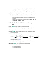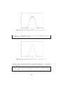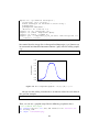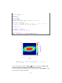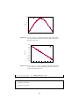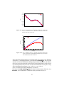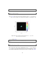
1
ECHO-QGP manual Version 1.0.00 The ECHO-QGP developers team 22-05-2015 Contents 1 Introduction 1.1 What is ECHO-QGP . . . . . . . . . . . . . . 1.2 The ECHO-QGP team . . . . . . . . . . . . . 1.3 License . . . . . . . . . . . . . . . . . . . . . 1.4 Funding . . . . . . . . . . . . . . . . . . . . 1.5 Main limitations - what the code cannot do . . . . . . . . . . . . . . . . . . . . . . . . . 3 3 3 4 5 5 . . . . . . . . . . . . . . . . . . . . . . . . . 2 How to set up and run simulations 2.1 Requirements . . . . . . . . . . . . . . . . . . . . . . . 2.1.1 Parallel run requirements . . . . . . . . . . . . 2.2 Download of ECHO-QGP . . . . . . . . . . . . . . . . . 2.2.1 Check of the integrity of the file . . . . . . . . . 2.2.2 Uncompress the folder . . . . . . . . . . . . . . 2.3 Configure ECHO-QGP . . . . . . . . . . . . . . . . . . 2.4 How to build and run ECHO-QGP . . . . . . . . . . . . 2.4.1 Build and run on multi-processors architectures . . . . . . . . . . . . . . . . . . . . . . . . 7 . 7 . 8 . 8 . 8 . 9 . 10 . 10 . 11 3 ECHO-QGP configuration 3.1 The param.dat file . . . . . . . . . . . . . . . . . . . . . . . . 3.2 Kind of initialization . . . . . . . . . . . . . . . . . . . . . . . 3.3 Kind of simulation . . . . . . . . . . . . . . . . . . . . . . . . 3.4 Grid parameters: . . . . . . . . . . . . . . . . . . . . . . . . . 3.5 Time parameters . . . . . . . . . . . . . . . . . . . . . . . . . 3.6 Output parameters . . . . . . . . . . . . . . . . . . . . . . . . 3.7 Algorithm parameters . . . . . . . . . . . . . . . . . . . . . . 3.8 Collision parameters . . . . . . . . . . . . . . . . . . . . . . . 3.9 Initial conditions parameters . . . . . . . . . . . . . . . . . . . 3.10 Viscosity parameters . . . . . . . . . . . . . . . . . . . . . . . 3.11 Equation of State parameters . . . . . . . . . . . . . . . . . . 3.12 Glauber Monte Carlo initial conditions parameters . . . . . . . 3.13 Decoupling hypersurface parameters . . . . . . . . . . . . . . 3.14 Initialization with a custom energy or entropy density profile . 3.15 Section for simulations with "tilted" initial energy density profile 1 15 15 17 18 18 19 19 20 20 20 21 21 23 24 24 24 3.16 Printed variables in the output files . . . . . . . . . . . . . . . 25 3.17 Essential parameters for projectile nuclei . . . . . . . . . . . . 27 4 Available initialization alternatives 4.1 Initialization 0 - Geometric Glauber . . . . . . . . . . . . . . . 4.2 Initialization 1 - 2D shock tube . . . . . . . . . . . . . . . . . 4.3 Initialization 2 - 1D viscous shear flow . . . . . . . . . . . . . 4.4 Initialization 3 - Glauber-MonteCarlo . . . . . . . . . . . . . . 4.5 Initialization 4 - Viscous Gubser Flow . . . . . . . . . . . . . . 4.6 Initialization 5 - tabulated initial energy or entropy density profile . . . . . . . . . . . . . . . . . . . . . . . . . . . . . . . 4.7 Other parameters inside the code . . . . . . . . . . . . . . . . 4.8 Arguments passing . . . . . . . . . . . . . . . . . . . . . . . . 28 28 30 30 30 31 5 Post-processing tools 5.1 IDL/GDL scripts . . . . . . . . . . . . . . . . . . . . . . . . . . 5.2 Fortran utilities . . . . . . . . . . . . . . . . . . . . . . . . . . 5.3 The particle spectra production tool . . . . . . . . . . . . . . . 34 34 35 37 6 Tutorials 6.1 A 3D+1 simulation with Glauber model - test A 6.2 2D shock tube - test B . . . . . . . . . . . . . . 6.3 1D viscous shear flow test - test C . . . . . . . . 6.4 Gubser flow test - test D . . . . . . . . . . . . . 6.5 Initialization with a tabulated file - test E . . . . 6.6 Glauber Monte Carlo initialization - test F . . . 6.7 Run with “tilted” initial conditions - test G . . . . . . . . . . 39 39 51 56 56 60 62 64 7 Particle spectra production 7.1 hypersuface.f90 in ECHO-QGP . . . . . . . . . . . . . . . . 7.2 Particle spectra routines . . . . . . . . . . . . . . . . . . . . . 7.3 How to configure the particle production . . . . . . . . . . . . 7.3.1 ECHO-QGP related parameters . . . . . . . . . . . . . 7.3.2 Particle related parameters . . . . . . . . . . . . . . . 7.4 Input-Ouput . . . . . . . . . . . . . . . . . . . . . . . . . . . . 7.5 Parameters for the Monte Carlo production . . . . . . . . . . . 7.6 Examples of particles subset: . . . . . . . . . . . . . . . . . . . 7.6.1 Producing all available particles: listorseq=0 . . . . . 7.6.2 Producing an interval of listed particles: listorseq=1 . 7.6.3 Producing a detailed list of particles listorseq=2 . . . 7.6.4 Producing the standard subset of particleslistorseq=3 67 67 69 69 71 71 73 73 75 75 75 76 77 References 77 2 . . . . . . . . . . . . . . . . . . . . . . . . . . . . . . . . . . . . . . . . . . . . . . . . . 31 32 33 Chapter 1 Introduction 1.1 What is ECHO-QGP ECHO-QGP is a program used to model heavy-ions collisions. It solves numerically the viscous hydrodinamic equations in the Israel-Stewart theoretical frame [1] [2] in 2+1D or 3+1D in Bjorken coordinates, from the formation of quark-gluon plasma up to the freeze-out stage. The user can set up different initial conditions (Optical and Monte Carlo Glauber, as well as custom initial energy density profile) and he/she can also choose between both analytic and tabulated equations of state. The programming language chosen for ECHO-QGP is FORTRAN 2008. 1.2 The ECHO-QGP team At the time of release 1.0.00 (22-05-2015), the ECHO-QGP team is composed by: • Francesco Becattini - Univ. of Florence - INFN, Sect. of Florence Project coordinator [email protected] • Andrea Beraudo - INFN, Sect. of Turin Glauber-Monte Carlo initialization, testing, postprocessing routines [email protected] • Luca Del Zanna - Univ. of Florence - INAF, Arcetri Obs. - INFN, Sect. of Florence Author of the original ECHO code (http://www.astro.unifi.it/echo/), from which ECHO-QGP has been derived [email protected] 3 • Arturo De Pace -INFN, Sect. of Turin Geometric Glauber initialization, testing [email protected] • Alessandro Drago - Univ. of Ferrara - INFN, Sect. of Ferrara Consultant [email protected] • Gabriele Inghirami - FIAS, Goethe-Universität - Frankfurt am Main Maintainer of the hydrodynamical evolution part of the code [email protected] • Marzia Nardi - INFN, Sect. of Turin Consultant, testing [email protected] • Giuseppe Pagliara - INFN, Sect. of Ferrara Consultant [email protected] • Valentina Rolando - INFN, Sect. of Ferrara Maintainer of the freeze-out and particle spectra computation part of the code [email protected] Past collaborators: • Vinod Chandra Consultant for the second order viscous corrections We would like to thank also: P. Cea, J. Rizzo, L. Cosmai, R. Tripiccione for their help in building up the very first implementation of ECHO-QGP, A. Palmese, A.M. Marin Garcia, V. Gonzalez, D. Piagneri for their feedback as first users of the pre-release versions of the code, G. Denicol for useful inputs about the Gubser’s viscous flow test. 1.3 License The code is released under the GPL v. 2.0; please, read the file LICENSE.TXT contained into the source directory or have a look at: https://www.gnu.org/ licenses/gpl-2.0.html. 4 1.4 Funding The development of ECHO-QGP has been supported by the Italian Ministry of Education and Research grant PRIN 2009 “Il Quark–Gluon Plasma e le collisioni nucleari di alta energia”, by the INFN project RM31 and by funding from HIC for FAIR. 1.5 Main limitations - what the code cannot do The main limitations of the code are: • The code can describe one fluid only, expanding in “vacuum” (see next point about the “vacuum” term) • The code needs a minimum baseline for the value of the energy density of the order of 1 KeV for the inviscid case, and 0.1 - 1 MeV for the viscous case • The time derivatives have a limited (∼ first order) accuracy • Baryon charge evolution is properly treated only in the inviscid case; in the viscous case it only plays a numerical role, but it doesn’t have a physical meaning since there are some missing terms in the equations describing its evolution • To ensure the stability of the program, it is necessary to switch off the viscosity effects under a certain temperature (usually, less than 100MeV, i.e. well below the freezeout temperature, where the hydrodynamical description is not valid anymore) • If initial conditions are not very “smooth”, the program may crash before reaching the freezeout temperature (unfortunately, currently this happens quite often with Glauber-Monte Carlo initial conditions) • The correct parsing of the configuration parameters requires not to alter the structure of the files param.dat and settings.txt • The hypersurface computation always runs over a single core: it is not parallelized • The grid partitioning in runs exploiting MPI is limited to the x-axis only and the user can exploit a number of CPUs not exceeding one third of the cells along the x axis • I/O actions are performed by only a single processor 5 • The code does not yet take into account a post-hydro after-burner (any transport code or resonance decayer, rescatterings, etc) 6 Chapter 2 How to set up and run simulations 2.1 Requirements Some requirements are assumed in order to use ECHO-QGP v1.0: • a working GNU/Linux environment • a fortran 2008 compiler • the make utility • the tar utility • the gzip utility The current version was developed and tested with: • Debian 7.0 x86_64 equipped with the GCC 4.7.2 compiler • Ubuntu 14.04 amd64 equipped with the GCC 4.8.2 compiler The makefile provided within the package contains some of the most frequent flags used for specific architectures, so that an expert user can modify it at pleasure. Additionally, some the (optional) postprocessing tools require GDL (http: //www.gnudatalanguage.org) or IDLr (by EXELIS VIS) to be installed. Root access is not needed to compile or run the program. 7 2.1.1 Parallel run requirements To execute parallel runs of ECHO-QGP on multiple cores machines, an MPI library is also needed. The code has been tested using only the OpenMPI implementation of the Message Passing Interface (MPI) standard, version 1.6.5 (all versions from 1.3.x to 1.8.x should also work, but they were not tested). 2.2 Download of ECHO-QGP The latest version is downloadable from the official ECHO-QGP website: http://theory.fi.infn.it/echoqgp . From now on, <version> occurences refer to the version of the code on which we are working on (e.g. ECHO-QGP-<version>.tar.gz could be ECHOQGP-1.0.03 or ECHO-QGP-1.5.11). The version id is composed by three numbers: a change in the first number will correspond to deep changes in the structure of the code or in the physics that it handles, a change in the second number will reflect significant improvements or minor new features, changes in the third number are reserved to bug-fixes only. Only bug-fixing versions will not introduce incompatibilities with previous versions, while first and second digit new versions probably it will. 2.2.1 Check of the integrity of the file It is possible to check the source code tarball integrity: it is sufficient to download the corresponding md5sum checksum file and issue the command: md5sum −c ECHO−QGP−<v e r s i o n >. t a r . gz . md5sum which returns, on positive match: ECHO−QGP−<v e r s i o n >. t a r . gz : OK For any other return state, the user should download again the package. 8 2.2.2 Uncompress the folder To unpack the compressed archive containing the sources, just issue the command: t a r x z f ECHO−QGP−<v e r s i o n >. t a r . gz The uncompressed folder will contain: some sub-directories for utilities and post-hydro programs, some text files and all the files building ECHO-QGP itself. In detail, the bundle is composed as follows: analysis folder Contains the post-hydro tools for the particle spectra production (see 7) doc folder Contains the latest version of this manual and the LATEX sources to build it eos_data folder Contains some essential files to run the simulations (equation of state, particle list, chemical potential, temperature definition . . . ) LICENSE.TXT text file License under wich ECHO-QGP is released. makefile The instructions to build the program using GNU Make param.dat text file Configuration file of ECHO-QGP random_seed.dat An integer number to provide an initial seed for the Random Number Generator (used with Glauber-Monte Carlo initial conditions) (see 4.4) tests folder Contains the essential informations and data to reproduce the examples described in the tutorials chapter (see 6) of this manual tools folder Contains some tools to analyze the results of the simulations (see 5) The remaining files included are the Fortran files containing the modules of ECHO-QGP. We give here an extremely synthetic description of each one of them: common.f90 contains all the global variables and some utility functions echo.f90 main file eos.f90 handles the Equation of State and the interplay among the thermodynamic variables evolve.f90 Computes the time evolution of the quark-gluon plasma 9 glaubermc.f90 Prepares the initial state for the hydro evolution with the Glauber Monte Carlo model holib.f90 Library with high order reconstruction algorithms hypersurface.f90 Computes the thermal freezeout hypersurface init.f90 Initialization file out.f90 Handles the output parallel_mpi.f90 Handles the parallelization parallel_nompi.f90 Dummy file for the serial run system.f90 Prepares the lattice and the metrics, handles the conversions between primitive and conserved variables viscous.f90 Computes the viscous corrections work.f90 Riemann solver and interfaces to high order libraries 2.3 Configure ECHO-QGP The configuration file param.dat can be edited with any text editor (e.g. vim, gedit, geany, kate. . . ), but it is very important NOT TO ALTER the structure of the file (number of columns before the = symbol or before the ! symbol). The change in the parameters in param.dat are read at runtime, so it is not necessary to compile again the program. There are some parameters that, as for now, are not configurable from the param.dat file, as they are declared in the Fortran files and their modification requires to recompile the program. See section 4.7 for further details. 2.4 How to build and run ECHO-QGP To build the program, enter the source directory and issue the command: make The command make reads the instructions on how to compile from the file makefile. The make command can be invoked with five different targets: make to build the program for serial runs on a single processor make par to build the program parallel runs on multi-cores systems using the MPI library 10 make tools to build the post-processing utilities contained into the tools directory make clean to remove the files produced during a previous compilation (executable, object files, modules and so on) make cleanall to remove both the files produced by the compiler and the files produced by an ECHO-QGP run An expert user can edit the makefile to change or choose a proper compiling option, suitable for its own compiler and architecture. On a successful build, the executable file echo.exe can be found in the directory. To run the program, simply issue: . / echo . exe 2.4.1 Build and run on multi-processors architectures If the user has a computer with many CPUs and the MPI library installed, he/she can speed up the simulations launching parallel runs. In order to compile ECHO-QGP with MPI, just issue the command: make par and then to run ECHO-QGP: mpirun −np <number o f p r o c e s s o r s > . / echo . exe ( e . g . mpirun −np 4 . / echo . exe ) where the -np flag sets up the number of processors to be used (to be more precise, the number of processes, but usually the best choice is to insert the number of CPUs available). Please, note that the minimum allowed number of cells along x is the number of processors divided by 3. The output files are stored in the outr0001 subdirectory. The output directory can be changed passing the -o flag to ECHO-QGP: / echo . exe −o new_name The name of the output directory must be 8 characters long. When performing Glauber-Monte Carlo simulations, the suffix numbers of output directories are automatically assigned: they will be equal to the index numbers identifying the selected events (for example, if the users chooses 11 to run events with id 113 and 114 in the sequence generated by ECHO-QGP, then the output directories will be outr0113 and outr0114). When correctly executed, ECHO-QGP prints a summary of the grid, the parameters and the algorithms employed, and then a short message each time the output is written and a final message about time elapsed. You can see an example of a successful running output (up to the second time-step in the listing 2.1) 1 3 ECHO - QGP STARTED nrk 5 7 9 11 13 15 17 19 21 23 25 27 29 31 33 35 : 2 **** Settings and parameters : **** Test 0 *** optical - geometrical Glauber initial Using Bjorken coordinates This is a viscous simulation Bulk viscosity is neglected This simulation uses MPI and the number 4 Evolved shear viscous tensor components : xx , yy , zz , xy , xz tt , tx , ty , tz and zz are obtained imposing orth . and null trace Grid parameters : x , y and z ( or eta ) number of cells : 51 x range ( fm ) : 9.000 y range ( fm ) : 9.000 z ( or eta ) range ( fm ) : 9.000 step x ,y , eta ( fm ) : 0.353 0.353 51 -9.000 -9.000 -9.000 0.353 Time parameters : starting time : ending time : ending temeperature ( MeV ) : maximum timestep : 1.000 1.400 130.000 0.005 eta / s parameter for shear viscosity tens Temperature limit for smoothing viscosit eq of state numerical derivatives with anal . eos 0.080 0.095 3 0 Nucleus parameters : proj . mass radius ( fm ) W . - S . width ( fm ) 197.000 6.380 0.535 12 51 47 sqrt ( s ) ( GeV ) Y_b cross section ( mb ) impact parameter ( fm ) initial hardness parameter central energy density ( GeV / fm ^3) enezero ( GeV / fm ^3) przero ( GeV / fm ^3) central density pp rapidity distribution shift ( deta - e pp rapidity distribution width ( sigeta p 200.000 5.361 4.200 5.000 0.150 20.000 0.10 E -02 0.22 E -03 0.100 1.000 1.500 49 ueta A coeff . so that u ^ eta = A * x : 0.000 Computing freeze - out hypersurface Hypersurface computation based on temper Freezeout threshold ( MeV ) : time interval between hypersurfaces comp 140.000 0.050 37 39 41 43 45 51 53 55 57 59 61 63 65 67 69 71 73 75 77 79 81 83 85 87 89 Other numerical parameters : Courant - Fr . - Lew . condition parameter : Reconstruction algorithm : Limiter : z - step thickness function ( fm ) r - step thickness function ( fm ) integration accuracy Output parameters : interval between log updating : interval between output printing : output precision : Variables printed in the output files : density vx vy vz pressure energy density temperature entropy density bulk viscosity pi ^ tt pi ^ tx pi ^ ty pi ^ tz pi ^ xy pi ^ xz pi ^ yz pi ^ xx pi ^ yy pi ^ zz u0 or gamma Lorentz factor 13 0.200 0.001 0.001 0.10 E -06 MPE5 MM2 0.010 0.050 double - 8 bytes 91 93 95 97 99 101 103 105 107 109 dutdt duxdx duydy duzdz theta or expansion rate vorticities will also be printed into separated output files Calculating thickness function ... check nucleus mass 196.94642 Done ! ************** RUN NUMBER 1 - RUN 1 OF 1 Initializations done ... mkdir outr0001 / Grid computed ... Files for hypersurface computation written ... Summary of variables written ... Time : 1.00000000 - out0001 . dat 1.61100000 secs Copying param . dat into the output directory ... Pressure treshold ( GeV / fm ^3) : 2.9468165948506055 E -003 Energy density treshold ( Gev / fm ^3) : 1.3051308079431541 E -002 Time : 1.05000000 - out0002 . dat 1.01000000 secs Listing 2.1: Output of ECHO-QGP 14 Chapter 3 ECHO-QGP configuration 3.1 The param.dat file The param.dat file contains several parameters used by the program and that the user can modify. Changing a parameter in such file does not imply to compile again ECHO-QGP, because the file is read during the execution of the program. Instead, if the analytical Equation of State (EoS) is modified, then it becomes compulsory to issue the command make clean before compiling ECHO-QGP again (because the files containing the analytical EoS are included with the include statements, thus they are not automatically considered by the make command). An example of param.dat is reported in the paragraph 3.1. This file has different sections, for different subsets of parameters used by different modules of the program. We are going to see them in detail in this section, following the file sections. Once again, it is very important NOT TO ALTER the structure of the file (number of columns before the = symbol or before the ! symbol). 2 4 6 8 10 12 14 ! kind of initialization INIT_TYPE =0 ! kind of simulation COORD ....=2 VISCOUS ..=0 BULK .....=0 NS .......=0 CUT_TEMP .=0.08 ! grid parameters NX .......=101 NY .......=101 NZ .......=101 XMIN .....= -12. XMAX .....=12. YMIN .....= -12. ! 0= Geometric Glauber , 1=2 D sh .. ! system coordinates : 1= Minkow ... ! it takes into account viscou ... ! if 0 it cuts off bulk viscos ... ! if 0 it uses I - S second orde ... ! if > 0 it fixes the temperat ... ! number of cells along x dire ... ! number of cells along y dire ... ! number of cells along z ( Min ... ! minimum value for x ! maximum value for x ! minimum value for y 15 16 18 20 22 24 26 28 30 32 34 36 38 40 42 44 46 48 50 52 54 56 58 60 62 64 66 68 YMAX .....=12. ! maximum value for y ZMIN .....= -12. ! minimum value for z ( Minkows ... ZMAX .....=12. ! maximum value for z ( Minkows ... ! time parameters TSTART ...=1.0 ! start simulation proper time ... TSTOP ....=10. ! stop simulation proper time ... TEMP_END .=.135 ! simulation ends when maximum ... ! output parameters DTLOG ....=0.05 ! proper time interval between ... DTOUT ....=0.1 ! proper time interval between ... OUTP_PREC =8 ! output precision : it can be ... MAXDT ....=0.01 ! maximum timestep ... RESTART ..=1 ! restart possibilities : 0= nev ... ! algorithm parameters CFL ......=0.2 ! Courant - Fr . - Lew . condition ... ! beam parameters NUCLEUS ..= Au ! symbol of the colliding ions ... RADS .....=200. ! sqrt ( s_NN ) ( GeV ) SIGMA_IN .=42. ! total inelastic cross sectio ... B ........=7. ! impact parameter ( fm ) ! initial conditions IENENTR ..=0 ! initial condition : 0 ( energy ... AH .......=0.15 ! initial hardness ECENTER ..=20. ! energy dens . or entropy dens ... ENEZERO ..=0.0000001 ! minimum value of energy dens ... RHOCENTER =0.1 ! charge density at the origin ... DETA .....=1.0 ! shift of the pp rapidity dis ... SIGETA ...=1.5 ! width of the pp rapidity dis ... ! viscosity parameters ( active only when VISCOUS paramete ... ETA_S ....=0.08 ! eta / entropy dens . parameter ... TAU_PI_C .=3. ! relaxation time coefficient ... TRACE_IMP = zz ! shear viscous tensor compone ... ! equation of state EOS ......=3 ! 1= analytic eos pr ( rh , en ) , 2=... TAB_EOS_FILE = qcdIEOS0 . dat ! name of the file containing ... NUM_DER ..=0 ! 1= with an . eos it uses num d ... ! section for Glauber MonteCarlo initial conditions ... NCONF ....=500 ! number of nuclear configurat ... NBCOLL ...=20 ! number of impact parameters ... EV_START .=28 ! identifies the event from wh ... EV_STOP ..=31 ! identifies the event at whic ... KAPPA ....=37.0 ! model parameters ( taken from ... SIG ......=0.6 ! smearing parameter COLLISION =1 ! kind of collision : 1= AA , 2= d ... ! section for freezout hypersurface computation HYP_COMPU =0 ! 0 disable / 1 enable hypersu ... FREEZKIND =0 ! 0 freezout based on temperat ... FREEZEVAL =.140 ! freezeout threshold : tempera ... HYPSURFTI =0.1 ! time interval between hypers ... ! section for initialization with an energy or entropy de ... IN_D_FILE = ed . dat ! name of the file with the ta ... ! section for simulations with " tilted " initial energy de ... ETAM_TILT = -1 ! eta_m to produce initial en .... UETA_COEF =0. ! for tests with initial u ^ eta ... 16 70 72 74 76 78 80 82 84 86 88 90 92 94 96 98 100 102 104 106 108 **************************************** ! Printed variables in the output files ( please , select 1... density ..=1 vx .......=1 vy .......=1 vz .......=1 ! vz obviously means veta when ... pressure .=1 ene_dens .=1 temper ...=1 entr_dens =1 bulk_visc =1 ! bulk viscosity , active only ... pi ^ tt ....=1 ! tt component of shear viscos ... pi ^ tx ....=1 ! tx component of shear viscos ... pi ^ ty ....=1 ! ty component of shear viscos ... pi ^ tz ....=1 ! tz component of shear viscos ... pi ^ xy ....=1 ! xy component of shear viscos ... pi ^ xz ....=1 ! xz component of shear viscos ... pi ^ yz ....=1 ! yz component of shear viscos ... pi ^ xx ....=1 ! xx component of shear viscos ... pi ^ yy ....=1 ! yy component of shear viscos ... pi ^ zz ....=1 ! zz component of shear viscos ... gamma ....=1 dutdt ....=0 duxdx ....=0 duydy ....=0 duzdz ....=0 theta ....=0 vorticity =0 ! prints the derivatives of va ... flows ....=0 ! prints directed and elliptic ... **************************************** ! Essential parameters for some nuclei . ! Please , add custom nucleus parameters paying attention ... ! When echo - qgp is launched , it will select the parameter ... Au Pb Xx000 Au000 - projmass =197. projmass =208. projmass =280. projmass =197. - radius =6.38 radius =6.62 radius =8.76 radius =6.37 ( fm ) ( fm ) ( fm ) ( fm ) - delta =0.5... delta =0.5... delta =0.7... delta =0.5... Listing 3.1: Example of param.dat 3.2 Kind of initialization This section is devoted to the pre-hydro modules, and it can set-up the initial energy density (or entropy density) profile in such a way that it reproduces a known test, or situation. See chapters 4 and 6 for the various initializations that can be reproduced with ECHO-QGP. 17 INIT_TYPE integer- flag. It is the flag selecting among different initial profiles, for a variety of cases. The allowed possibilities are (see next chapter 4): 0. Glauber-geometric initialization 1. 2D shock tube test 2. 1D viscous shear flow test 3. Glauber-Monte Carlo initialization 4. viscous Gubser’s fluid test 5. Initialization with a tabulated energy or entropy density profile 3.3 Kind of simulation This section is devoted the set-up of the simulation, such as choosing the coordinates (see also 4). COORD integer- flag. It sets the metric used: 1. Minkowski coordinate system with metric diag(-1,1,1,1) 2. Bjorken coordinate system, with metric diag(-1,1,1,τ 2 ) VISCOUS integer- flag. Enables (1) or disables (0) the viscous correction to the evolution equations. BULK integer- flag. Enables (1) or disables (0) the bulk viscosity contribution. In the first case the parameter ζ = 2η(1/3 − cs2 ), in the last ζ = 10−40 NS integer- flag. If set to 1 it imposes the use of Navier-Stokes formalism instead of the I-S second order theory CUT_TEMP real, flag and cutoff. If > 0 then under the temperature CUT_VALUE the viscous tensor components are "smoothed", i.e. their magnitude is reduced This section is devoted the set-up of the lattice 3.4 Grid parameters: NX integer- value. The number of cells along x direction NY integer- value. The number of cells along y direction NZ integer- value. The number of cells along eta direction. To set up 2D+1 simulations, just impose NZ=1. XMIN real- value. The minimum value for x 18 XMAX real- value. The maximum value for x YMIN real- value. The minimum value for y YMAX real- value. The maximum value for y ZMIN real- value. The minimum value for z (or η) ZMAX real- value. The maximum value for z (or η) 3.5 Time parameters The simulation starts at a given proper time and can be terminated by two different criteria: when it reaches a threshold temperature or at a given proper time. TSTART real- value. Proper time at which the simulation starts (τ0 in fm/c) TSTOP real- value. Proper time at which the simulation ends (in fm/c) TEMP_END real- flag and cutoff. The simulation ends when the maximum temperature in GeV reaches a value less than TEMP_END. If this parameter is set to 0, then this feature is turned off. 3.6 Output parameters This section specifies the output frequency and criteria. DTLOG real- value. Proper time interval between log updating (it should be greater than MAXDT) DTOUT real- value. Proper time interval between output printings (it should be greater than MAXDT) OUTP_PREC integer- flag. The user can choose between 4 (single) or 8 (double) bytes precision when printing output values. Note that in the particle-production tools, this choice is made at build time. MAXDT real- value. Maximum time-step allowed for the time-integration. RESTART integer- flag. Enables (1) or disables (0) the possibility to restart a simulation from the last output file. If enabled, it forces the frequency of output printing and freeze-out hypersurface computation to be done at the same time. 19 3.7 Algorithm parameters CFL real- value. The Courant–Friedrichs–Lewy condition 3.8 Collision parameters In this section ECHO-QGP reads all the parameters characterizing the collision: the specie of the nuclei, the beam energy . . . NUCLEUS character- flag. It sets the specie of colliding nuclei, and it corresponds to the symbol of the atom (e.g. Au or Pb). At the end of the file param.dat the essential parameters corresponding to each nucleus are written, i.e. mass in a.m.u., radius in f m, Wood-Saxon width in f m and normal nuclear density in f m−3 . The user can add other species simply appending other data with the same format at the end of the file. RADS real- value. Total energy per nucleon in the center of mass frame √ ( sN N ), in GeV SIGMA_IN real- value. The total inelastic nucleon-nucleon cross section, in mb B real- value. The impact parameter b, expressed in fm. 3.9 Initial conditions parameters IENENTR integer- flag. Allows to use either energy (0) or entropy (1) density for the profile used in the initial stage modeling. AH real- value. Hardness parameter αBC ∈ [0, 1], in equation 4.1. ECENTER real- value. Central (x = y = z = b = 0) value for the field used in the initial profile, i.e.: For IENENTR=0, ECENTER is the energy density in GeV/fm3 For IENENTR=1, ECENTER is the entropy density in fm−3 ENEZERO real- value. Minimum allowed value for the energy density, in GeV/fm3 , at program starting RHOCENTER real- value. Central (x = y = z = b = 0) value for the baryon charge density in f m−3 . Please, note that in the current version, this parameter does not have any physical meaning: it is exploited as a tracer (i.e. as a mathematical trick to simplify the evolution equations of shear viscous tensor components). In order to perform viscous simulations RHOCENTER must be different from zero. 20 DETA real- value. Shift of the pp-rapidity distribution (ηf lat in equation 4.1) SIGETA real- value. Width of the pp-rapidity distribution (ση in equation 4.1) 3.10 Viscosity parameters These parameters are only considered when the flag VISCOSITY=1. ETA_S real- value. It is the shear viscosity coefficient divided by the entropy density: η/s (in natural units). It is employed in the calculation of the shear viscous tensor, where s is the entropy density. In the Navier-Stokes formulation, this value is simply assigned to η. TAU_PI_C real- value. The parameter which controls the τπ , the relaxation time, in the formula: τπ = T AU _P I_C ETTA_S , where T is the temperature TRACE_IMP character- flag. Discriminates the equation used to close the system. It can assume two different values: TRACE_IMP=no The components π xx , π yy ,π zz ,π xy ,π xz ,π yz of the shear viscous tensor are evolved, while the π tt ,π tx ,π ty ,π tz components are retrieved imposing the orthogonality condition; TRACE_IMP=zz the π zz component is obtained imposing the tracelessness condition (in addition to the orthogonality condition) 3.11 Equation of State parameters EOS integer- flag. Discriminates the Equation of State used by ECHO-QGP. The options are: 1. A barotropic analytic equation of state is used, of the kind (P = P (ρ, e)). The relations among the pressure (P ), the charge density (ρ) and energy density (e) are explicitly written in the files .def contained in the folder eos_data: pressure_vs_rh_en.def Dependence of the pressure (P, GeV /f m3 ) on the energy density (e, GeV /f m3 ) temperature.def Dependence of the temperature (T, GeV) on the energy density (e, GeV/fm3 ) energy_den.def (Optional, only if NUM_DER=0) the dependence of energy density on pressure dprdrh.def (Optional, only if NUM_DER=0) the partial derivative of pressure respect to density 21 dprden.def (Optional, only if NUM_DER=0) the partial derivative of pressure respect to energy density The files in the bundle contain the ideal ultrarelativistic EoS P = e/3. More precisely, P = e/3 = gπ 2 T 4 , 90 (~c)3/4 1 c2s = , 3 where g = 37 for a non-interacting QGP with 3 light flavors. All the *.def files in the eos_data folder can be edited as the user wishes, as long as the variable and parameters names are preserved. Any change in these files requires to issue again the command make. 2. A complete analytic equation of state, with the pressure as a function of temperature (T) and chemical potential (µ) is used (P = P (T, µ)). This feature is not yet implemented in the current version of the code. 3. ECHO-QGP uses a tabulated equation of state, specified in the file TAB_EOS_FILE. 4. ECHO-QGP builds a tabulated equation of state and then uses it ( Feature not yet implemented in this version of the code ) TAB_EOS_FILE character(max 15 characters). Name of the file containing the tabulated EoS (if EOS=3), to be located in the eos_data directory. ECHO-QGP allows the use of any tabulated EoS of this kind, if provided by the user in the following format: • The first row containing the number N of entries of the file. • N rows, each one containing: the temperature T in GeV , the energy density in GeV /T 4 , the pressure in GeV /T 4 , the square speed of sound cs 2 ≡ dP/de; all separated by white spaces In the bundle, there are four available tabulated EoS files: qcdIEOS.dat EoS of ref. [3], arising from a weak-coupling QCD calculation with realistic quark masses qcdIEOS0.dat Nearly identical to qcdIEOS.dat, except for the first entry for T=0 (added to solve some stability problems at low temperatures, far below the temperature range of existence of the quark-gluon plasma). pce.dat EoS of ref. [4], based on partial chemical equilibrium obtained by matching a Hadron-Resonance-Gas EoS (HRG EoS) at low temperature with the continuum-extrapolated lattice-QCD results by 22 the Budapest-Wuppertal collaboration [5]. The HRG EoS was obtained by summing the contributions of all Phadrons and resonances in the PDG up to a mass of 2 GeV: P = r Pr . pce0.dat The same as pce.dat, but with an additional entry for T=0. NUM_DER integer- flag. Enables or disables the automatic computation of the derivatives for the thermodynamic variables, in case of an analytic EoS. Works with EOS=1 or EOS=2. • ECHO-QGP computes numerical derivatives to find other physical quantities • The user must provide explicit derivatives in the files energy_den.def and part_der_pr_vs_rh_en.def 3.12 Glauber Monte Carlo initial conditions parameters NCONF integer- value. Number of nuclear configurations NBCOLL integer- value. Number of impact parameters per configuration EV_START integer- ID. ID number of the event from which to start among the generated events EV_STOP integer- ID. ID number of the event from which to stop among the generated events KAPPA real- value. Value of the K parameter in: " # ) Npart N coll 2 coll )2 X X (x − xpart ) K (x − x i i e(τ0 , x) = . (1 − α) exp − +α exp − 2πσ 2σ 2 2σ 2 i=1 i=1 For further details see [6, 7] SIG real- value. Value of the σ (smearing) parameter in the above equation. For further details see [6, 7] COLLISION integer- flag. Discriminates the kind of collision • 1=AA (nucleus-nucleus) • 2=dA (deuton-nucleus) • 3=pA (proton-nucleus) 23 3.13 Decoupling hypersurface parameters The task of the routine hypersuface.f90 included in ECHO-QGP is to find, store and print the coordinates of the hypersurface detected during the hydrodinamic evolution. HYP_COMPU integer- flag. Disables (0) or enables (1) the computation of the decoupling hypersurface. If set to 0, it saves computational time but it does not perform any decoupling technique. FREEZKIND integer- flag. Criterion for the detection of the hypersurface. 0. Isothermal hypersuface - Uses a threshold temperature (FREEZEVAL= Tf o , GeV) 1. Constant energy density hypersuface - Uses a threshold energy density (FREEZEVAL= ef o , GeV/fm3 ) FREEZEVAL Decoupling field threshold: temperature (GeV ) or energy density (GeV /f m3 ) HYPSURFTI real- value. Time interval (in fm/c) of the grid passed to the hypersurface-finding routine. Sometimes to treat shocks it is useful to set a very dense grid, but in order to compute the hypersurface a lesser dense grid is needed, so it would be a waste of computing time to perform the check at every hydro step. 3.14 Initialization with a custom energy or entropy density profile ECHO-QGP can use as a starting profile (τ = τ0 ) a custom 2D energy density or entropy density profile at mid-rapidity, with the field values at any cell center. The structure of the file must be: x coordinate, y coordinate, energy density value in GeV/fm3 or entropy density value in fm−3 . The field values of the tabulated file will be interpolated on the grid chosen in param.dat if the grid on which they lie does not match with the grid of ECHO-QGP. IN_D_FILE character(max 18 characters). Name of the file with the tabulated energy or entropy density distribution (max 18 characters) 3.15 Section for simulations with "tilted" initial energy density profile ETAM_TILT real- value. Parameter to produce a “tilting” in the initial energy distribution as in ref. [8]; if the parameter is set to a negative number, no tilting is introduced 24 UETA_COEF Parameter used for tests with initial conditions different from the BIC (uη = ux = uy = 0). Here uη 6= 0, and uη (x) = UETA_COEF ·x (the impact parameter b lies on the x axis). 3.16 Printed variables in the output files This section simply contains a list of all the fields that the simulation can print in the output files. The user can enable (1) or disable (0) the output of any variable. The computational time also depends on how many variables are printed. They all are real- flags - with the precision defined by the flag OUTP_PREC. density (baryon charge density) vx (vx contravariant) vy (vy contravariant) vz (vz or vη contravariant) pressure (p, expressed in GeV/fm3 ) ene_dens (e, energy density, expressed in GeV/fm3 ) temper (T , temperature, expressed in GeV) entr_dens (s, entropy density, expressed in fm−3 ) bulk_visc Π (bulk viscosity, only active when VISCOUS parameter is set to 1) pitt π tt component of shear viscous tensor, active only when VISCOUS parameter is set to 1 pitx π tx component of shear viscous tensor, active only when VISCOUS parameter is set to 1 pity π ty component of shear viscous tensor, active only when VISCOUS parameter is set to 1 pitz π tz component of shear viscous tensor, active only when VISCOUS parameter is set to 1 pixy π xy component of shear viscous tensor, active only when VISCOUS parameter is set to 1 pixz π xz component of shear viscous tensor, active only when VISCOUS parameter is set to 1 25 piyz π yz component of shear viscous tensor, active only when VISCOUS parameter is set to 1 pixx π xx component of shear viscous tensor, active only when VISCOUS parameter is set to 1 piyy π yy component of shear viscous tensor, active only when VISCOUS parameter is set to 1 pizz π zz component of shear viscous tensor, active only when VISCOUS parameter is set to 1 gamma γ Lorentz factor (also vt ) ∂vt ∂t dutdt duxdx ∂vx ∂x duydy ∂vy ∂y duzdz ∂vz ∂z ∂v y ∂vx ∂vz t theta θ = ∂v ∂t + ∂x + ∂y + ∂z with Minkowski coordinates and the τ additional term uτ with Milne coordinates derivativ Prints the derivatives of velocities and temperature vs τ ,x,y and η at τ intervals given by parameter DTOUT into separate output ASCII files der0001.dat, der0002.dat, ... and, if the computation of f.o. hypersurface is active, also on f.o. hypersurface, producing the file hypersurf_deriv.txt flows Prints the hydrodynamical eccentricities on the transverse plane vs η at τ intervals given by parameter DTOUT into separate output ASCII files df0001.dat, ep0001.dat, ec0001.dat, df0002.dat, ep0002.dat, ec0002.dat, .... The computations are valid only in the inviscid case. The definition we used for the spatial eccentricity ec0... files is: R dxdy(x − x0 )2 − (y − y0 )2 εc (η)const.τ = R dxdy(x + x0 )2 − (y + y0 )2 the definition for the df0... files with average flow in x direction is: R dxdyγvx hvx i (η) = R dxdyγ while the definition [9] for the momentum eccentricity ep0... files is: R dxdy( + p) · γ 2 · (vx2 − vy2 ) εp (η)const.τ = R dxdy( + p) · γ 2 · (vx2 + vy2 ) + 2 · p 26 where is the energy density, γ is the Lorentz factor and p is the pressure. 3.17 Essential parameters for projectile nuclei In this section it is possible to choose the parameters for specific nuclei and/or to give the essential parameters (i.e. mass in a.m.u., radius in fm, Wood-Saxon width in fm and normal nuclaer density in fm−3 ). If a new projectile nucleus is wanted, it is sufficient to type (or copy and paste) a new line, where the 5 characters at the beginning are reserved for the name and the rest of the line structure is preserved. 27 Chapter 4 Available initialization alternatives As its hydrodynamic starting point, ECHO-QGP can set up different initial energy density (or entropy density) profiles, based on various widespread models or on some of the most common numerical tests. The ones currently available in the code are listed below and they are selected through the parameter INIT_TYPE in the configuration file param.dat. 4.1 Initialization 0 - Geometric Glauber Here we compute the initial state for the energy density profile in the Optical Glauber Model frame [10]. We define the usual thickness function as: Z ∞ ρ0 √ T (x, y) = dz x2 +y 2 +z 2 −r −∞ δ 1+e where ρ0 , δ and r are the normal nuclear density, the Wood-Saxon width and the radius of the nucleus (all of them defined at the end of param.dat file). Then we define: T− (xT ) = T (xT − b/2) T+ (xT ) = T (xT + b/2) where xT = (x, y) is the vector of the transverse plane coordinates and b is the impact parameter vector, connecting the centers of the two nuclei. In our conventional cartesian reference frame, the b vector is oriented along the positive x axis and the two nuclei have initial momentum along the z axis (whence the reaction plane is the xz plane). b is assigned with the B parameter. Given: σ as the total nucleon-nucleon inelastic cross section (corresponding 28 to the parameter SIGMA_IN), m as the mass number of the colling nuclei and T (x, y) as the thickness function, we define: σT+ m σT− m T1 (x, y) = T+ 1 − 1 − T2 (x, y) = T− 1 − 1 − m m while the number of binary collisions is: nBC (x, y) = σT+ (x, y) T− (x, y) We define the wounded nucleons weight function WN as: WN (x, y, η) = 2 (T1 (x, y)f− (η) + T2 (x, y)f+ (η)) where: and 1 −η + η m f− (η) = 2ηm 0 0 η + η m f+ (η) = 2η m 1 η < −ηm −ηm ≤ η ≤ ηm η > ηm η < −ηm −ηm ≤ η ≤ ηm η > ηm Finally, the initial proper energy density distribution is assumed to be: ε(x, y, η) = ε0 W (x, y, η) H(η), where ε0 is assigned with the parameter ECENTER and the total weight function W (x, y, η) is defined as: W (x, y, η) = (1 − α) WN (x, y, η) + α nBC (x, y) . (1 − α) WN (0, 0, 0) + α nBC (0, 0) where α is the AH parameter and: η̃ 2 H(η) = exp − 2 θ(η̃) 2ση η̃ = |η − η0 | − ηf lat /2 where η0 = 0 if the parameter ETAM_TILT > 0 (“tilted initial energy profile”), otherwise: 1 1 + β0 η0 = ln 2 1 − β0 where β0 = T− − T+ T− + T+ 29 Viscous tensor components are initialized as: 2η = g11 3 τ0 2η π 22 = g22 3 τ0 4η π 33 = −g33 3 τ0 ζ Π=− τ0 All other components are set to 0. π 11 4.2 Initialization 1 - 2D shock tube Initial condition is a constant pressure profile p1 for y ≤ −x and p2 otherwise. All other variables are set to 0. The inital values of the variables can be changed only editing the init.f90 file (and recompiling ECHO-QGP). 4.3 Initialization 2 - 1D viscous shear flow These initial conditions are designed to perform the (1+1)-D test in Minkowski Cartesian coordinates described in [6] and [11]. Pressure and density have constant values (density ρ = 1 and pressure p = 0.25 so that, using ideal equation of state!energy density e = 3p = 0.75 x p and e + p = 1), and v y = v0 · erf , where the constant v0 c 2 t · η/s and t is time (with this choice of the various parameters, t should be 1 at the beginning of the simulation). 4.4 Initialization 3 - Glauber-MonteCarlo This initialization is based on a simple Glauber MonteCarlo model, designed as follows [7] [6]: • A Woods-Saxon distribution is sampled to create an initial nuclear configuration. The transverse positions of the nucleons of the two colliding nuclei are reshuffled into their center-of-mass frame. • For each configuration a random impact parameter b ∈ [0, bmax ] is extracted from the distribution dP = 2πbdb. A collision happens if the positions xi of the nucleon i (from nucleus A) and xj of nuclean j (from nucleus B) are such that: (xi −xj )2 +(yi −yj )2 < σN N /π. The parameter min_participants (contained into file glaubermc.f90) establishes the minimum number of particpant nucleons to accept or reject the 30 event. The user, with the parameter NCONF, can choose how many configurations to compute. • To each participant and collision is associated an energy density distribution described by a gaussian function with variance σ; these distributions are then summed together: # " ) Npart N coll 2 coll )2 X X (x − xpart ) (x − x K i i +α exp − . e(τ0 , x) = (1 − α) exp − 2πσ 2σ 2 2σ 2 i=1 i=1 • The profile e(τ0 , x) is then multiplied by 0 |η| ≥ ybeam 2 η̃ ηf lat ≤ |η| < ybeam f (η) = exp − 2 2ση 1 |η| < ηf lat where η̃ = |η| − ηf lat /2, ηf lat is given, in √ param.dat, by the DETA SN N parameter, ση by SIGETA and ybeam = log mN • Viscous tensor components are initialized as in initialization 0. We advice that, at the time of the release of ECHO-QGP 1.0.00 , initializations with p+A and d+A collisions have not been properly tested. 4.5 Initialization 4 - Viscous Gubser Flow Viscous Gubser flow with initial values provided by a tabulated file named Initial_Profile_GubserFlow.dat contained into the main ECHO-QGP source tree. This is a 2D+1 test in Bjorken coordinates. See the proper section 6.3 in the tutorials chapter for further informations. 4.6 Initialization 5 - tabulated initial energy or entropy density profile This is a 2D+1 initialization. Inital energy density profile (if parameter IENENTR is set to 0) or entropy density profile (if parameter IENENTR is set to 1) are read from file named IN_D_FILE. Viscous tensor components are initialized as in initialization 0. 31 4.7 Other parameters inside the code The user can change some parameters included inside the code. After changing one of these parameters, the user has to recompile the code before using the program. If the user changes files with definitions like eos_data/temperature.def, which are inserted into other source files by an include directive, he/she has also to clean the source tree with make clean or make cleanall before recompiling the program with make or make par. option_algo Parameter located into system.f90, inside the subroutine system_cons2prim, it changes the algorithm for obtaining primitive variables starting from the evolved conservative ones. The best choice is usually 1. lambda0, lambda1, lambda2 Parameters located into system.f90, inside the subroutine system_sources, they enable (if set to 1.) or disable (if set to 0.) the contributions to the source terms of viscous tensor components of: the − 43 π µν θ term, the second order terms, the vorticity terms. iseed Parameter saved into the file random_seed.dat. When using GlauberMC initialization procedure, if ECHO-QGP finds this file, it reads the integer value it contains for seeding the random number generator, thus reproducing the last energy density profile. If the user removes this file, ECHO-QGP uses the integer value obtained from a system_clock call as the new random seed iseed and it saves its value inside the file random_seed.dat. REC Choice of reconstruction algorithm (also used for computing spatial derivatives of velocities for obtaining shear viscous tensor components). Possibile choices are: TVD2, CENO3, WENO3, WENO5, PPM4, MPE3, MPE5, MPE7. This parameter is located inside common.f90. limiters The tvd2, ceno3 and ppm4 reconstruction algorithms may use MM2 or MC2 as possible limiters. The pre-defined algorithm is MM2, but the user can change it to MC2 commenting/uncommenting just a few lines inside holib.f90 following the instructions inserted into the code. If the user wishes to change how the values of viscous tensor are initialized, he/she has to modify the final part of the subroutine viscous_initio, contained into file viscous.f90. If the user wishes to change the initial uη velocity field, he/she has to modify the subroutine calc_vel_long_nz_ueta, contained into the file init.f90. The parameter η0 as defined into 4.1 can also be changed editing the function H_of_eta into the file init.f90. 32 4.8 Arguments passing ECHO-QGP accepts some arguments passed when calling it. Currently they are: -v, –version it prints version information and exits -h, –help it prints usage information (this message) and exits -m, –maxdt maximum timestep allowed -r, –restart it restarts from last saved frame -t, –tstop n it ends at proper time tstop -o, –outdir name it changes the name of output directory 33 Chapter 5 Post-processing tools Inside the tools directory there are several utilities to manipulate the results to make easy to visualize them using programs like grace, IDL/gdl or gnuplot: 5.1 IDL/GDL scripts readvar.pro IDL/GDL script that reads the output of echo-qgp and stores the variables it into 3-dimensional arrays, the grid data into 3 arrays x, y and z. The files grid_summary.dat and param.dat must be in the same directory with data where this script is launched. readvartime IDL/GDL script that reads the output files of echo-qgp and the values of a chosen variable at a chosen point on the grid in a chosen range of output files are printed into a chosen file togheter with the time at which they refer. The files grid_summary.dat and param.dat must be in the same directory with data where this script is launched. readder.pro IDL/GDL script that reads the output files of echo-qgp containing data about variable derivatives at fixed τ . The files grid_summary.dat and param.dat must be in the same directory with data where this script is launched. ce.pro IDL/GDL script that, for the inviscid case and Bjorken coordinates only, computes the total energy Etot and the total angular momentum J zx along the y direction over the computational grid using the formulas: Z Etot = τ (cosh T 00 − sinh T z0 )dηdxdy J zx Z = τ (cosh η(zT 0x − xT 0z ) − sinh η(zT zx − xT zz ))dηdxdy 34 Since the energy density value defined by the ENEZERO parameter is added to each cells of the grid at the beginning of each run with Glauber initial conditions, the values of these “basement” energy density and the corresponding pressure can be assigned to the limit_en and limit_pr variables (in the first lines of the script) before running the script, so that they will be subtracted. These values of limit_en and limit_pr variables are printend to the standard output by ECHO-QGP at the beginning of each run. Please, note that this utility is based on a raw summation of the values inside the cells and, depending on what are the grid dimensions, the grid resolution and the value of ENEZERO, it may give inaccurate or even wrong results. You are invited to always check the results changing grid dimensions, grid resolution and the value of ENEZERO. 5.2 Fortran utilities readx.f90 this small program can be individually compiled with the command: gfortran -o readx.exe -fdefault-real-8 readx.f03 . The synopsys of the program is: ./readx.exe number_of_start_frame number_of_end_frame If selected in the param.dat file (and, for viscous tensor components, if we run a simulation with viscosity), there will be the following output files (nnnn refers to the four digits number identifying the frame): • EPSnnnn.dat - the energy density • PRnnnn.dat - the pressure • VXnnnn.dat - the velocity along x direction • VYnnnn.dat - the velocity along y direction • VZnnnn.dat - the velocity along η direction • RHOnnnn.dat - the charge density • Snnnn.dat - the entropy density • Tnnnn.dat - the temperature • bulknnnn.dat - the bulk viscosity • ttnnnn.dat - the π tt shear viscous tensor component • txnnnn.dat - the π tx shear viscous tensor component • tynnnn.dat - the π ty shear viscous tensor component • tznnnn.dat - the π tz shear viscous tensor component • xynnnn.dat - the π xy shear viscous tensor component • xznnnn.dat - the π xz shear viscous tensor component 35 • yznnnn.dat - the π yz shear viscous tensor component • xxnnnn.dat - the π xx shear viscous tensor component • yynnnn.dat - the π yy shear viscous tensor component • zznnnn.dat - the π zz shear viscous tensor component • x.dat, y.dat, eta.dat, tau.dat - the grid coordinates fromecho.f90 this small program can be individually compiled with the command: gfortran -o fromecho.exe -fdefault-real-8 fromecho.f90 . The synopsis of the program is: ./fromecho input_file output_file x|y|z. The program takes as input one of the output files of readx and select the values of the given variables along the x, y or z direction from the 0 up to the right border, printing them into output_file. For example: ./fromecho.exe PR0001.dat pressure.txt x it will print into the file pressure.txt the values of pressure along x from 0 up to the border of the grid. The ouput file is a two column ascii file, in the first column there are the coordinate values and in the second column the variable values. fromecho2d.f90 this utility extracts a 2D slice parallel to one of the coordinate axis from a 3D set of data. It can be individually compiled with the command: gfortran -o fromecho2D.exe -fdefault-real-8 fromecho2D.f90 and its synopsis is: /fromecho input output x|y|z x|y|z (optional: x|y|z value, default is 0) where input is one of the files containing single variable data produced by readx. Usage example: ./fromecho prova_input prova_output x y This extracts data from file prova_inputs and writes into file output_file the values on the x-y plane for z=0 Usage example: ./fromecho prova_input prova_output z x 5 This extracts data from file prova_inputs and writes into file output_file the values on the z-x plane for y=5 For the optional 5th argument, actually it is selected the grid value which is closest to the chosen value , i.e. no interpolations are made. The ascii output file contains the coordinate value on the first axis, the coordinate values on the second axis and the variable value in that point of the slice. Assuming that these values are x,y and f(x,y), the output file is written in this way: 36 x(1) y(1) f(x(1),y(1)) x(1) y(2) f(x(1),y(2)) x(1) y(3) f(x(1),y(3)) ... ... ... x(1) y(ny) f(x(1),y(ny)) blank line x(2) y(1) f(x(2),y(1)) x(2) y(2) f(x(2),y(2)) ... ... ... x(2) y(ny) f(x(2),y(ny)) blank line x(3) y(1) f(x(3),y(1)) x(3) y(2) f(x(3),y(2)) ... ... ... ... ... ... x(nx-1) y(ny) f(x(nx-1),y(ny)) x(nx) y(ny) f(x(nx),y(ny)) The blank lines are inserted to make easier to plot the output file with gnuplot. timev.f90 this small program can be individually compiled with the command: gfortran -o timev.exe -fdefault-real-8 timev.f90 . Usage example: ./timev.exe T 1 137 51 40 37 pippo It prints into the file named "pippo" two columns of values: the first one contains the time, the second one the values of the variable (usually T stands for temperature) at cell of indexes x 51, y 40 and z 37 stored in the files from T0001.dat to T0137.dat search.sh This very small and very simple bash script searches and highlights a given string inside all source code files. Example: ./search.sh allocate 5.3 The particle spectra production tool The tool for producing particle spectra is contained into the analysis directory and can be compiled simply with the make command. This program is able to use OpenMP for speeding up computations in system with multicore processors with shared memory (and, of course, with OpenMP installed). To take advantage of OpenMP, you have to edit the makefile adding the compilation flag -fopenmp and execute the make command (you just have to comment/uncomment a couple of lines at the beginning of the makefile). If 37 compilation is successfull, export the environment variables used by OpenMP (unless they have already been set up in advance), e.g., for a 4 cores cpu: e x p o r t OMP_NUM_THREADS=4 e x p o r t OMP_SCHEDULE=GUIDED , 4 At the end of the compilation stage, you’ll get an executable named thermal.exe. When OpenMP is used, if thermal.exe is the only relevant running application, the common top utility will report for thermal.exe a %CPU usage almost equal to OMP_NUM_THREADS times 100. The configuration file is settings.txt. The output directory where the program stores the results must be created before launching it. For a much more detailed description of this tool, please, read chapter 7. 38 Chapter 6 Tutorials In this chapter we will give some examples of how to use the code. The tutorials will not cover all the features of ECHO-QGP, nevertheless they should give to the user a working knowledge sufficient to perform many basic tasks. Usage examples of external programs like gnuplot or the gnudatalanguage will be provided, too, hoping that they will be useful to young students and to other people not familiar with them. The tests directory contains the configurations files and some plots (together with related datafiles) of the results of the numerical simulations presented in this chapter. 6.1 A 3D+1 simulation with Glauber model - test A Unpack the code with: t a r x f echo−qgp−<v e r s i o n >. t a r . gz Then, enter into the code directory: cd echo−qgp−<v e r s i o n > If you wish, you can modify the makefile to best exploit the capabilities of your processor or for debugging purposes. Default optimization flag -O2 should fit well for most cases. If your cpu has only one core or if you wish to run ECHO-QGP serially, to compile just issue: make 39 otherwise, with a multi-core machine with MPI installed, issue: make par Now, open the file param.dat with your favorite text editor (e.g. vim, emacs, gedit, geany, kwrite, kate...). Let’s assume that we wish to run a 3D+1 simulation of the hydrodynamical p evolution of the QGP after the collision of two gold nuclei at an (sN N ) = 200 GeV using Geometrical Glauber Initial conditions with an impact parameter of 7 fm, taking into account shear viscosity effects with an η/s = 0.08. We choose 140 MeV as freeze-out temperature. The details of ECHO-QGP configuration are all written into the param.dat file inside the folder tests/testA. Assuming that we have got a two core computer, we’ll use: mpirun −np 2 . / echo . exe or, if we have got only a single core machine (and so, obviously, we didn’t choose to use mpi): . / echo . exe If we wish to run the program even after we log out from the computer (very common situation when we use an ssh connection), we may use nohup: nohup mpirun −np 2 . / echo . exe& With nohup, the messages printed by echo-qgp on the screen will be written into a file named nohup.out. The output data files will be written into the outr0001 directory; inside that directory a log file showing the progress of the computation will be updated every DTLOG τ intervals (in this example run, each 0.01 fm/c). Let’s suppose, now, that the run ended and we wish to analyze the results. First, we need to compile the fortran postprocessing utility with the command: make t o o l s and then we have to copy the produced executable files (with the .exe extension) and the GDL scripts into the output directory: cp t o o l s / * . exe t o o l s / * . pro outr0001 40 Now, let’s move into the output directory: cd outr0001 If you have installed IDL or its free clone named gnudatalanguage (at least, version 0.9.3, its website is: http://gnudatalanguage.sourceforge.net), you can use some scripts to make some sketchy, but quick plots. Let’s see how. First, launch gdl: gdl You’ll get an interactive shell. With the script readvar.pro you will be able to read the variables of the output and manipulate them interactively. First, we check if initialization was correct, so we read the first output file: GDL> readvar , 0001 % Compiled module : READVAR . T h i s program r e a d s t h e ou t pu t o f echo−qgp Reading grid_summary . dat nx : 101 ny : 101 nz : 101 xstep : 0.277228 − y s t e p : 0.277228 − z s t e p : 0.277228 xmin : −14.0000 − ymin : −14.0000 − zmin : xmax : 14.0000 − ymax : 14.0000 − zmax : Reading g r i d . dat % Compiled module : SKIP_LUN . Run with v i s c o s i t y Output has 8 bytes precision V a r i a b l e s t o be read : density vx vy vz pressure energy d e n s i t y temperature entropy density bulk v i s c o s i t y p i^t t p i^t x p i^t y p i^t z p i^xy p i^xz p i^yz p i^xx 41 −14.0000 14.0000 p i^yy p i^zz gamma Number o f v a r i a b l e s i s : 20 Reading f i l e : out0001 . dat time : 1.00000000 time ( or tau ) i s s t o r e d i n t o v a r i a b l e t= 1.0000000 A r r a y s a v a i l a b l e : x , y and z o f t y p e double with 101 101 101 elements A r r a y s a v a i l a b l e with t h e i r maximum , mean and minimum v a l u e s : % Compiled module : MEAN. rho : 0.10000000 0.10000000 0.10000000 vx : 0.0000000 0.0000000 0.0000000 vy : 0.0000000 0.0000000 0.0000000 vz : 0.0000000 0.0000000 0.0000000 pr : 3.9807911 0.030049485 6.1038367 e−05 en : 15.303008 0.13728677 0.00030000000 temp : 0.30648078 0.057427603 0.047645369 entropy : 62.920094 0.69550263 0.0075776172 bu : 0.0000000 0.0000000 0.0000000 tt : 0.0000000 0.0000000 0.0000000 tx : 0.0000000 0.0000000 0.0000000 ty : 0.0000000 0.0000000 0.0000000 tz : 0.0000000 0.0000000 0.0000000 xy : 0.0000000 0.0000000 0.0000000 xz : 0.0000000 0.0000000 0.0000000 yz : 0.0000000 0.0000000 0.0000000 xx : 0.66217778 0.0073195439 7.9747652 e−05 yy : 0.66217778 0.0073195439 7.9747652 e−05 zz : −0.00015949530 −0.014639088 −1.3243556 v0 : 1.0000000 1.0000000 1.0000000 It is usually a wise practice not only to check what ECHO-QGP prints to the standard output, but also that the simulation has been properly initialized and the gdl scripts offer a good method to test it. We can easily check, for example, grid dimensions, grid resolution and what variables will be printed into the output files. Also, we can check that initial velocities are all 0 and that the minimum value of π ηη is twice the maximum value of π xx and π yy with changed sign, while other shear viscous tensor components are 0. It is beyond the scope of this tutorial to teach how to use gdl (or IDL), however we’ll give some additional basic information to show how to make some sketchy plots. Further informations can be easily found on the web.1 Using gdl it possible to store the data as multidimensional arrays into the RAM of the computer and then extract, print and plot some sections of them. 1 See, for example: http://www.ita.uni-heidelberg.de/~dullemond/lectures/num_fluid_2009/App_B. pdf or http://www.sgeier.net/tools/GDL-intro.pdf 42 In gdl array indexes start from 0 and intervals are denoted by colons; the arguments of the functions are separated by commas. So, for example, to print to print the first four values of the x array: GDL> p r i n t , x ( 0 : 3 ) −13.861386 −13.584158 −13.306931 −13.029703 To make things faster, you can move across the history of commands using the keyboard arrows and re-edit the commands. Dimensions inside multi-dimensional arrays are separated by commas. The asterisk means “all elements contained into that dimension”. We can assign the values of a slice of an already existing array to a new array, for example the following energy_for_z_0 array contains the value of energy density for η = 0: GDL> e n e r g y _ f o r _ z _ 0=reform ( en ( * , * , 5 0 ) ) GDL> help , e n e r g y _ f o r _ z _ 0 ENERGY_FOR_Z_0 DOUBLE = Array [101 , 101] The help command tells what kind of values its argument is; please, remind that gdl is case insensitive (.i.e. “a” and “A” are the same variable). Here we used reform to cut off the dimension with only 1 element. In this particular case, actually it was not needed, but it is recommended to always use it when you wish to cut slices with less dimensions to avoid to get 3D objects instead as 2D, as in this case: GDL> e n e r g y _ t r y=en ( * , 5 0 , * ) GDL> help , e n e r g y _ t r y ENERGY_TRY DOUBLE = Array [101 , 1 , 101] To make a plot, we can type: GDL> p l o t , x , e n e r g y _ f o r _ z _ 0 ( * , 5 0 ) , x t i t l e ="x ( fm ) " , y t i t l e =" Energy d e n s i t y (GeV/fm^3) " , psym=2, xrange =[−10,10] and a plot like that in Fig. 6.1 will appear on a separate window (actually, here we show a postscript figure created with a couple of additional commands, see further in this text; plots on the screen usually have b/w colors inverted). If we didn’t plot the x array together with the en slice, then gdl on the x axis would have used only the index numbers of the elements of the slice of the en array. Let’s see now how the energy density profile looks like moving along the η direction at x=y=0 (Fig. 6.2): 43 Figure 6.1: Plot of energy density in GeV /f m3 at τ = 1 f m/c for y = η = 0. GDL> p l o t , z , en ( 5 0 , 5 0 , * ) , x t i t l e =" e t a " , y t i t l e ="Energy d e n s i t y ( GeV/fm^3) " , xrange =[−10,10] Figure 6.2: Plot of energy density in GeV /f m3 at τ = 1 f m/c for x = y = 0. Now let’s make a surface plot of the energy density along the x − η plane for y = 0 (Fig. 6.3): GDL> s u r f a c e , reform ( en ( * , 5 0 , * ) ) , x , z , x t i t l e ="x ( fm ) " , y t i t l e =" e t a " , z t i t l e ="En . dens . (GeV/fm^3) " , xrange =[ −10 ,10] , yrange =[−10,10] 44 Figure 6.3: Surface plot of energy density in GeV /f m3 at τ = 1 f m/c for y = 0. Let’s replot the same quantities, but using a contour plot (Fig. 6.5): GDL> s e t _ p l o t , ’ ps ’ GDL> d e v i c e , f i l e n a m e =" p l o t 4 . ps " GDL> contour , reform ( en ( * , 5 0 , * ) ) , x , z , x t i t l e ="x ( fm ) " , y t i t l e =" e t a " , xrange =[ −6 ,6] , yrange =[ −5 ,5] , LEVELS = [ 0 . 0 , 2 . 5 , 5 . , 7 . 5 , 1 0 . , 1 2 . 5 , 15 , 1 7 . 5 , 2 0 . ] , C_LABELS = [ 1 , 0 , 1 , 0 , 1 , 0 , 1 , 0 , 1] GDL> d e v i c e , / c l o s e Now, let’s have a look at what is the situation at a later time, using the fortran utilities. Output data are written into binary files; the readx.exe utility extracts these data into separate files for each variable in ascii format. Calling readx.exe without any argument prints an help message: . / readx . exe P l e a s e , i n s e r t t h e range o f echo−qgp ou t pu t f i l e s from which you want t o e x t r a c t v a l u e s . ( O p t i o n a l l y , you can a l s o w r i t e t h e name o f t h e d i r e c t o r y where t h e ou t pu t f i l e s w i l l be w r i t t e n ) ( d e f a u l t : p o s t p r o c / readx ) If we are interested only in output at τ = 10.0 f m/c, we can look at the time.dat file and, after reading that corresponding output data number is 91, we can type: 45 Figure 6.4: Contour plot of energy density in GeV /f m3 at τ = 1 f m/c for y = 0. . / readx . exe 91 91 time= 9.9999999999999822 If we wished to extract all output data from τ = 4.5 f m/c to τ = 4.8 f m/c we would use: . / readx . exe 36 39 time= 4.5000000000000009 time= 4.6000000000000005 time= 4.7000000000000002 time= 4.7999999999999998 Now, we copy the utility fromecho.exe into the new created postproc/readx directory and then we enter into it: cp fromecho . exe p o s t p r o c / readx cd p o s t p r o c / readx Calling fromecho.exe without any arguments prints an help message: 46 . / fromecho . exe Synopsis : To e x t r a c t data from t h e l e f t t o t h e r i g h t b orde r o f t h e g r i d along x , y or z d i r e c t i o n : . / fromecho i n p u t _ f i l e o u t p u t _ f i l e x| y | z To e x t r a c t data u s i n g a s p e c i f i c range along one d i r e c t i o n and f i x i n g t h e o t h e r ones a t a p o i n t : . / fromecho i n p u t _ f i l e o u t p u t _ f i l e x| y | z x−indx−s t a r t x−indx−end y −indx−s t a r t y−indx−end z−indx−s t a r t z−indx−end P l e a s e , note t h a t s t a r t i n g and ending i n d e x e s o f t h e f i x e d d i r e c t i o n s must be e q u a l Usage example : . / fromecho p r o v a _ i n p u t p r o v a _ o u t p u t y 33 33 2 150 44 44 T h i s e x t r a c t s data from f i l e p r o v a _ i n p u t s and w r i t e t h e v a l u e s along y d i r e c t i o n from p o i n t with index 2 t o p o i n t with index 150 , f i x i n g x a t index 33 and z a t index 44 We extract the value of temperature at τ = 10 f m/c along the x axis for y = η = 0: . / fromecho . exe T0091 . dat temperature_x_tau_10 . 0 . dat x Now extract the value of temperature at τ = 10 f m/c along the η axis for x = y = 0, for all the η range (reminding that now indexes go from 1 to 101): . / fromecho . exe T0091 . dat t e m p e r a t u r e _ z _ t a u _ 1 0 . 0 . dat z 51 51 51 51 1 101 All the files created by fromecho.exe consists of two columns: the first one is the coordinate position, the second one the value of the variable. This data format can be easily read by many plotting software. For example, using gnuplot (Fig. 6.5): gnuplot G N U P L O T Version 4.6 p a t c h l e v e l 0 B u i l d System : Linux x86_64 l a s t m o d i f i e d 2012−03−04 C o p y r i g h t (C) 1986−1993, 1998 , 2004 , 2007−2012 Thomas Williams , C o l i n K e l l e y and many o t h e r s g n u p l o t home : faq , bugs , e t c : immediate h e l p : h t t p : / /www. g n u p l o t . i n f o t y p e " h e l p FAQ " t y p e " h e l p " ( p l o t window : h i t ’h ’ ) Terminal t y p e s e t t o ’ wxt ’ gnuplot> s e t term pos eps c o l enh f o n t " H e l v e t i c a , 22" Terminal t y p e s e t t o ’ p o s t s c r i p t ’ 47 O ptions a r e ’ eps enhanced d e f a u l t p l e x \ leveldefault color colortext \ dashed d a s h l e n g t h 1 . 0 l i n e w i d t h 1 . 0 b u t t n o c l i p \ nobackground \ palfuncparam 2000 ,0.003 \ " H e l v e t i c a " 22 f o n t s c a l e 1 . 0 ’ gnuplot> s e t out " t e m p e r a t u r e . eps " gnuplot> s e t y l a b e l " Temperature (GeV) " gnuplot> s e t x l a b e l " { / Symbol h } " gnuplot> p l o t " . / t e m p e r a t u r e _ z _ t a u _ 1 0 . 0 . dat " with l i n e s p o i n t s l t 7 linecolor 3 notitle We remind that the image files in Encapsulated Postscript (.eps) format can be converted into Portable Document Format (.pdf) with the utility ps2pdf, e.g.: ps2pdf −dEPSCrop t e m p e r a t u r e . eps 0.16 Temperature (GeV) 0.14 0.12 0.1 0.08 0.06 0.04 0.02 -15 -10 -5 0 5 10 15 η Figure 6.5: Test A - Temperature profile at τ = 10 f m/c for y = η = 0. We can use the utility fromecho2d.exe to extract values for a 2D slice of the grid, for example: . / fromecho2d . exe T0091 . dat tempxz91 . dat x z Then, we can use a gnuplot script like the following to plot the data: # S e t t e r m i n a l and o ut pu t s e t t e r m i n a l p n g c a i r o s i z e 900 , 900 enhanced f o n t ’ H e l v e t i c a , 2 2 ’ s e t encoding u t f 8 s e t ou t pu t ’ contour91xz . png ’ 48 # Set p l o t p r o p e r t i e s s e t s i z e square s e t pm3d unset surface s e t view map s e t key o u t s i d e s e t pm3d i n t e r p o l a t e 0 ,0 # i n t e r p o l a t e t h e c o l o r # Set the c o l o r p a l e t t e s e t p a l e t t e model RGB d e f i n e d ( 0 ’ b l a c k ’ , 1 ’ b l u e ’ , 2 ’ cyan ’ ,3 ’ green ’ ,4 ’ y e l l o w ’ , 5 ’ red ’ , 6 ’ p u r p l e ’ ) # Se t h e axes s e t x l a b e l ’ x ( fm ) ’ s e t y l a b e l " {/ Symbol h} " s e t c b l a b e l " Temperature (MeV) " # Draw t h e p l o t s p l o t ’ tempxz91 . dat ’ u 1 : 2 : ( $3 * 1000.) n o t i t l e Figure 6.6: Test A - Contour of temperature (MeV) at τ = 10 f m/c for y = 0. A copy of the plotted datafile tempxz91.dat can be found in tests/testA. Now let’s see how to compute the thermal particle spectra. From the ECHO-QGP main directory of sources we enter the analysis subdirectory and we compile the tools: 49 make We remind that, to make use of OPENMP, the user has to edit the makefile and export some environment variable, see 5.3 for more details. Using the following configuration file settings.txt: ! T h i s i s t h e f i l e c o n t a i n g t h e s e t t i n g s f o r t h e r o u t i n e producing the s p e c t r a ! *** ECHO−RELATED dim . . . . . . = 3 ! 1+1, 2+1, 3+1 dimension f o r t h e s i m u l a t i o n v i s c o _ h y d=1 ! I s i t a v i s c o u s hydro s i m u l a t i o n ? 0=no , 1=y e s v i s c o _ s p e=1 ! viscosity corrections t o t h e d i s t r i b u t i o n f u n c t i o n ? 0=no , 1=y e s v o r t i c i t y =0 ! E v a l u a t e v o r t i c i t y on hypersurface nout . . . . . = 0 ! t o t a l number o f outputs ( i f 0 reads a l l a v a i l a b l e ) ! *** PARTICLE−RELATED npt . . . . . . = 4 0 ! points f o r the t r a n s v e r s e momentum ptmin . . . . = 0 . 0 ! min t r a n s v e r s e momentum ptmax . . . . = 4 . 0 ! max t r a n s v e r s e momentum nphi . . . . . = 3 6 ! p o in ts f o r the polar angle phimin . . . = 0 . 0 ! min p o l a r a n g l e phimax ...=6.28318530718 ! max p o l a r a n g l e nrap . . . . . = 4 1 ! p o in ts f o r the particle rapidity rapmin ...= −4.0 ! min r a p i d i t y rapmax . . . = 4 . 0 ! max r a p i d i t y l i s t o r s e q =2 ! 0− a l l ; 1−sequence I D _ s t a r t −I D _ s t o p ; 2− l i s t ; 3− s t a b l e I D _ s t a r t .=211 ! ID o f f i r s t p a r t i c l e t o be c o n s i d e r e d I D _ s t o p ..=−10213 ! ID o f l a s t p a r t i c l e t o be c o n s i d e r e d p a r t _ l i s t =2 ! p a r t i c l e s in the l i s t 211 3122 a n t i b a r ..=1 ! 1=on 0=o f f chempot ..=1 ! read c h e m i c a l p o t e n t i a l from . . / e o s _ d a t a / c h e m i c a l _ p o t e n t i a l . t x t ; 0 s t e mu=0 ! *** INPUT i n p u t d i r . = . . / outr0001 / ! input directory i o u t d i r . . = . . / outr0001 / s p e c t r a / ! o u tp ut d i r e c t o r y f i l e . . . . . = out ! name o f t h e ECHO outout f i l e 50 ! *** RANDOM SEED ( saved anyway ) seed . . . . . = 0 seed , o t h e r w i s e use t h a t ptbox . . . . = 3 . 0 phibox . . . = 0 ybox . . . . . = 0 0 . 0 ! *** HISTOGRAM−RELATED mxv_pt . . . = 3 . 0 mnv_pt . . . = 0 . 0 mxv_ang ..=6.28318 mnv_ang . . = 0 . 0 mxv_y . . . . = 0 . 0 mnv_y . . . . = − 0 . 0 binpt ....=50 binphi ...=1 binrap ...=1 6.28318530718 ! i f 0 g e n e r a t e s random ! upper l i m i t f o r mc box ! i f 0 i s 2* p i ! upper l i m i t f o r mc box ! ! ! ! ! ! ! ! ! max min max min max min value value value value value value for for for for for for pt pt phi phi y y we can compute the thermal spectra of π + , Λ0 and Λ0 , taking into account the viscous corrections to the distribution function. Please, remember to create the outr0001/spectra directory before running the tool. After executing the program: . / thermal . exe we can enter into outr0001/spectra and make some plots: g n u p l o t p l o t _ p i o n p l u s _ s p e c t r a . gp The plot files can be quickly converted from EPS to PDF with f o r i i n * . eps ; do ps2pdf −dEPSCrop $ i ; done (See figures 6.7,6.8,6.9,6.10). 6.2 2D shock tube - test B This is a simple test of a 2D shock wave. The param.dat files of this test can be found into the tests/testB directory. The initial state is simply costitued by a sharp jump in pressure when crossing the y = −x locus, whose values can be adjusted editing the init.f90 file a few lines after the condition: 51 90 f0+df f0 80 70 R(y) 60 50 40 30 20 10 -4 -3 -2 -1 0 1 2 3 4 y Figure 6.7: Test A - dN dy of π + particles. Red color means that viscous corrections to thermal distribution have been taken into account, blue color means not. 1000 f0+df f0 100 I(pT, y=0) 10 1 0.1 0.01 0.001 0.0001 1e-05 0 0.5 1 1.5 2 2.5 3 3.5 4 pt [GeV] Figure 6.8: Test A - I(pT , y = 0) of π + particles. Red color means that viscous corrections to thermal distribution have been taken into account, blue color means not. e l s e i f ( i n i t _ t y p e . eq . SHOCK_TUBE_2D) then i f ( y ( i y ) . l t . −x ( i x ) ) then vv ( kpr ) =5.401411 else vv ( kpr ) =0.337588 end i f 52 0.02 f0+df f0 0.015 0.01 v1(y) 0.005 0 -0.005 -0.01 -0.015 -0.02 -4 -3 -2 -1 0 1 2 3 4 y Figure 6.9: Test A - Directed flow of π + particles. Red color means that viscous corrections to thermal distribution have been taken into account, blue color means not. 0.4 f0+df f0 0.35 v2(pT, y=0) 0.3 0.25 0.2 0.15 0.1 0.05 0 0 0.5 1 1.5 2 2.5 3 3.5 4 pt [GeV] Figure 6.10: Test A - Elliptic flow of π + particles. Red color means that viscous corrections to thermal distribution have been taken into account, blue color means not. After compiling ECHO-QGP, we run ECHO-QGP a few times using different values for η/s, changing the ETA_S parameter into param.dat. We can also execute an inviscid simulation setting the parameter VISCOUS..=0. Please, take care to not overwrite the results of the various simulations, either renaming the output directory after the end of each simulation or using the -o flag when launching the program (e.g. ./echo.exe -o out_2Dtest). First, we check if the initial conditions are correct. We copy the tools/readvar.pro gdl script into the output directory (e.g. outr0001, but it could have a different name) and then we use it: 53 cd outr0001 gdl GDL> readvar , 0001 We can make a sketchy plot simply typing: GDL> p l o t , x , pr ( * , 1 0 0 ) This is fine to make a simple check, but, if we wish to prepare a better quality plot, we can export the data to a file and then use it another tool (e.g. gnuplot, grace and many others). To perform this task, we can use the fortran postprocessing tools or gdl itself, preparaing, for example, a script like (file tests/testB/tofile.pro): openw , 12 , " i n i t i a l _ p r e s s u r e _ t e s t B . dat " ; p l e a s e , change t h e f o r −c y c l e i n t e r v a l a c c o r d i n g l y with your g r i d ; remind t h a t a r r a y i n d e x e s i n gnudatalanguage s t a r t from 0 ; f o r example , i f you have a 201x201 g r i d , i n i t i a l and f i n a l v a l u e s a r e 0 and 200 ; and , i f t h e g r i d i s symmetric r e s p e c t t o t h e o r i g i n , t h e index c o r r e s p o n d i n g t o 0 i s 100 f o r i =0,200 do begin p r i n t f , 12 , x ( i ) , pr ( i , 1 0 0 ) endfor f r e e _ l u n , 12 END If we run the script with: GDL> . r t o f i l e we should get an ascii file called initial_pressure_testB.dat which we can plot using another program (6.11): Assuming to have executed four simulations, one inviscid and the other three with η/s = 0.001, 0.01, 0.1, after compiling the fortran tools and copying them into the output directory, we can extract the data at the end of the run (τ = 4 fm/c) with: . / readx . exe 31 31 54 6 Pressure (GeV/fm3) 5 4 3 2 1 0 -5 -4 -3 -2 -1 0 1 2 3 4 5 x (fm) Figure 6.11: Test B - Initial pressure profile at τ = 1, f m/c for y = 0. followed by (into the postproc/readx directory): . / fromecho . exe EPS0031 . dat en0_1 . dat x 1 201 101 101 1 1 . / fromecho . exe VX0031 . dat vx0_1 . dat x 1 201 101 101 1 1 In the previous example, the name of the output files refer to energy density and Vx of the run with η/s = 0.1. In the tests/testB directory there is a simple gnuplot script to plot the results after gathering them in a common directory (Fig. 6.12 and 6.13). 0.35 Inviscid η/s=0.001 η/s=0.01 η/s=0.1 0.3 Vx (c units) 0.25 0.2 0.15 0.1 0.05 0 -5 -4 -3 -2 -1 0 1 2 3 4 5 x(fm) Figure 6.12: Test B - Comparison of Vx profiles at τ = 4, f m/c for y = 0. 55 22 Inviscid η/s=0.001 η/s=0.01 η/s=0.1 Energy density (GeV/fm3) 20 18 16 14 12 10 8 6 4 2 -5 -4 -3 -2 -1 0 1 2 3 4 5 x(fm) Figure 6.13: Test B - Comparison of energy density profiles at τ = 4, f m/c for y = 0. 6.3 1D viscous shear flow test - test C This is merely the execution of the test described in section 4.3 and [6]. The file param.dat to set up the simulation can be found in tests/testC. The results can be examined with the usual tools, following the procedures already shown in the previous examples: . / readx . exe 91 91 . / fromecho . exe VY0091 . dat vy . dat x 1 301 1 1 1 1 A simple gnuplot script (plot1D.gp) to plot the results is also included. 6.4 Gubser flow test - test D The description of this test can be found on [12] [8], here we’ll simply summarize what do to perform it. First, we need a set of initial values, which can be found into the tests/testD directory. This file, named Initial_Profile_GubserFlow.dat, has been produced with Maple 12 executing the worksheet initial_conditions_maple12.mw contained into the same directory. The settings inside param.dat must match those of the tabulated initial conditions (e.g. the grid) and also τπ , η/s and the relation between temperature and energy density must correspond to what chosen for computing the input file with initial conditions. The file tests/testD/param.dat works with the provided intial conditions. To complete the setup, the user has to comment/uncomment the temperature 56 0.01 0.008 0.006 ECHO-QGP Analytic 0.004 Vy 0.002 0 -0.002 -0.004 -0.006 -0.008 -0.01 -1.5 -1 -0.5 0 0.5 1 1.5 x Figure 6.14: Test C - Comparison between the analytical solution and ECHOQGP at τ = 10 fm/c. relation with energy density inside the eos_data/temperature.def file, clean the sources with make clean and recompile ECHO-QGP. If the grid used for computing the initial conditions is changed, then it is required to change not only the lines defining the grid into param.dat, but also the checks contained into init.f90 after the line with comment “! GUBSERCHECKS”. Since in this test we wish to compare the evolution of some variables with the semianalytical solutions obtained numerically with some external code, we need also these solutions. In the tests/testD directory we provide the solutions computed with Maple 12 at τ = 4 fm/c; the Maple worksheet can be reused, with only minor changes, to compute the solutions at different times and/or with different grid resolutions. After the end of the run, we can check the results. There are many ways to do it, here we’ll use gdl and gnuplot. cd outr0001 gdl We can use the shell commands inside gnudatalanguage adding a dollar ($) sign before issuing the command. For example, to list the files inside the current directory to check if the script readvar.pro is there we can type: GDL> $ l s −l | grep r e a d v a r −rw−r−−r−− 1 g g 12562 mag 9 02:42 r e a d v a r . pro 57 Now we read the output at τ = 4 fm/c (please, remind that you can look at time.dat to see what is the output number corresponding to that time). GDL> readvar , 0031 % Compiled module : READVAR . T h i s program r e a d s t h e ou t pu t o f echo−qgp Reading grid_summary . dat nx : 401 ny : 401 nz : 1 xstep : 0.0500000 − y s t e p : 0.0500000 − z s t e p : 2.00000 xmin : −10.0250 − ymin : −10.0250 − zmin : −1.00000 xmax : 10.0250 − ymax : 10.0250 − zmax : 1.00000 Reading g r i d . dat % Compiled module : SKIP_LUN . Run with v i s c o s i t y Output has 8 bytes precision V a r i a b l e s t o be read : density vx vy vz pressure energy d e n s i t y temperature entropy density bulk v i s c o s i t y p i^t t p i^t x p i^t y p i^t z p i^xy p i^xz p i^yz p i^xx p i^yy p i^zz gamma Number o f v a r i a b l e s i s : 20 Reading f i l e : out0031 . dat time : 4.00000000 time ( or tau ) i s s t o r e d i n t o v a r i a b l e t= 4.0000000 A r r a y s a v a i l a b l e : x , y and z o f t y p e double with 401 401 1 elements A r r a y s a v a i l a b l e with t h e i r maximum , mean and minimum v a l u e s : % Compiled module : MEAN. rho : 0.21052070 0.12870059 0.0034551016 vx : 0.97009619 8.2463097 e−16 −0.97009619 vy : 0.97009619 −6.2895014e−15 −0.97009619 vz : 0.0000000 0.0000000 0.0000000 pr : 0.0074253124 0.0010125367 1.0013452 e−05 en : 0.022275937 0.0030376102 3.0040355 e−05 temp : 0.059237610 0.027047653 0.011351802 58 entropy : 0.50139177 0.088629927 0.0035284097 bu : 0.0000000 0.0000000 0.0000000 tt : 0.0000000 −0.0011994727 −0.0089583879 tx : 0.0093095075 −3.2743781e−18 −0.0093095075 ty : 0.0093095075 −6.1862789e−18 −0.0093095075 tz : 0.0000000 0.0000000 0.0000000 xy : 0.0044716459 1.7072896 e−18 −0.0044716459 xz : 0.0000000 0.0000000 0.0000000 yz : 0.0000000 0.0000000 0.0000000 xx : 1.1768752 e−05 −0.00081962219 −0.0096843503 yy : 1.1768752 e−05 −0.00081962219 −0.0096843503 zz : 0.00010049364 2.7411661 e−05 −3.8899064e−07 v0 : 4.1203721 1.9250202 1.0000000 Now we read the tabulated file with the solutions computed by Maple using the script read_M12.pro, in the tests/testD directory: GDL> . r read_M12 % Compiled module : $MAIN$ . mx12 , my12 , mtemp12 , mux12 , muy12 , mpixx12 , mpiyy12 , mipxy12 , mpitt12 , mpitx12 , mpity12 , mpizz12 The script reads the file maple_gub_full_y_eq_x_tau_4.0; the user can easily modify the worksheet to read other files with the same structure. Now we prepare the data for plotting. We are interested in the values with coordinates x = y, so first we declare an array to store these values: GDL> a=d b l a r r (401) Then we fill the array, in this example with the values of ux = γv x : GDL> f o r i =0,400 do a ( i )=v0 ( i , i ) * vx ( i , i ) And now we print the values to compare into the file ux-comparison.dat: GDL> openw , 12 , " ux−comparison . dat " GDL> f o r i =0,400 do p r i n t f , 12 , x ( i ) , a ( i ) , mux12( i ) GDL> f r e e _ l u n , 12 Now we can make the plot with gnuplot: set set set set set term pos eps c o l enh f o n t " H e l v e t i c a , 2 2 " out " ux . eps " x l a b e l " x ( fm ) " y l a b e l " u^x ( c u n i t s ) " key top l e f t box 59 p l o t " ux_comparison . dat " u 1:2 w l l t 1 l c 3 lw 3 t i t l e "ECHO−QGP" , " ux_comparison . dat " u 1:3 w l l t 3 l c 4 lw 3 t i t l e " Semianalytic " The commands are gathered into the plot-ux.gp script under tests/testD, which can be executed with: g n u p l o t p l o t −ux . gp 3 ECHO-QGP Semianalytic 2 ux (c units) 1 0 -1 -2 -3 -10 -5 0 5 10 x (fm) Figure 6.15: Test D - Comparison between the semianalytical solution and ECHO-QGP results at τ = 4 fm/c. Into the tests/testD directory there are a few more plots of other variables, obtained with the same procedure. 6.5 Initialization with a tabulated file - test E In this kind of initialization, the initial entropy density distribution is provided with an ascii tabulated file. Changing the IENENTR parameter from 1 to 0, it is also possible to initialize ECHO-QGP using an energy density distribution. The name of the input file can be chosen with the IN_D_FILE parameter. The input file for this example is created with a short python script (init_tab.py) that computes a simple gaussian distribution. The script and the param.dat file to configure ECHO-QGP are into the tests/testE directory. See figures 6.16 and 6.17. 60 Figure 6.16: Test E - Initial energy density distribution at τ = 1 fm/c. Figure 6.17: Test E - Energy density distribution at τ = 5 fm/c. 61 6.6 Glauber Monte Carlo initialization - test F In the tests/testF directory can be found a param.dat file to initialize a Glabuer-Monte Carlo simulation. The random seed determines what will be the sequence of events, so, using the same random seed, saved into the file random_seed.dat, it is possible to reproduce the same initial series of events. Other parameters can be ajdusted editing the first lines of glaubermc.f90. In this example, we try to produce a series of events from a sequence of 500 nuclear configurations, each with 20 different impact parameters, getting 1881 events which satisfy our selection criteria (i.e., a minimum of 18 participants, as specified with the option min_participants=18 at the beginning of file glaubermc.f90). The results are stored into the file partcoll.dat. From this list, we select the event with id 67, but we can choose a sequence of events instead of a single one. Now we plot the initial energy density distribution. The procedure, for each plot, is the same, apart, obviously, for the names of the files. For the event with id 67: we compile the fortran prostprocessing tools: make t o o l s cp t o o l s / readx . exe outr0067 cd outr0067 We are interested in the first and last output files, so: . / readx 1 1 . / readx 94 94 cp . . / t o o l s / fromecho * . exe p o s t p r o c / readx cd p o s t p r o c / readx 62 . / fromecho2d . exe EPS0001 . dat en_out1 . dat x y g n u p l o t c o n t o u r _ o u t 1 . gp The Fig. 6.18 shows the initial energy distribution on the η = 0 (x,y) plane at τ = 1 fm/c. Now we look at the energy density profile as a function of η for Figure 6.18: Test F - Initial energy density distribution at τ = 1 fm/c with Glauber-MonteCarlo initialization. x = y = 0 (Fig. 6.19): . / fromecho . exe EPS0001 . dat e n e r g y _ v s _ e t a _ t a u 1 . dat z 56 56 56 56 1 81 g n u p l o t p l o t _ e n _ v s _ e t a . gp Now we plot the initial energy distribution on the η = 0 (x,y) plane at τ = 10.22 fm/c (last output frame before the end of the simulation, i.e. when the maximum temperature on the grid was less than 137 MeV) (Fig. 6.20). 63 50 45 40 35 30 25 20 15 10 5 0 -15 -10 -5 0 5 10 15 η Figure 6.19: Test F - Initial energy density vs η at τ = 1 fm/c and x = y = 0 (Glauber-MonteCarlo initialization). . / fromecho2d . exe EPS0094 . dat en_out94 . dat x y g n u p l o t contour_out94 . gp 6.7 Run with “tilted” initial conditions - test G In this example we run a simulation with Geometric Glauber initial conditions, without viscous effects, but with a “tilted” energy density distribution. The files related to this example can be found into the tests/testG directory. Using the same procedure shown in the previous example (test F), we draw a contour plot of the initial energy distribution, to visually verify the effect of “tilting” (Fig. 6.21). Now, since this is a simulation without viscosity effects, we use the GDL postprocessing utilities to verify the conservation of total energy and angular momentum during the fluid evolution. So, after copying from the tools directory into the outr0001 directory the readvar.pro and ce.pro scripts, we launch gdl and we run them: GDL> readvar , 0001 GDL> ce 64 Figure 6.20: Test F - Initial energy density distribution at τ = 10.22 fm/c with Glauber-MonteCarlo initialization. Figure 6.21: Test G - Initial energy density distribution at τ = 1 fm/c. getting, for tau = 1 fm/c: Total energy: 12400.207 65 J^y: -5838.3068 then, to see what are the total energy and the angular momentum J y at τ = 11 fm/c: readvar , 0101 ce getting: Total energy: 12371.264 J^y: -5834.8883 So, in this run, total energy was conserved within a ∼ 0.2% while , for J y , within a ∼ 0.06%. 66 Chapter 7 Particle spectra production We always refer to the Minkowski and Bjorken metrics respectively as 1 1 −1 −1 µν gM = g µν = (7.1) −1 −1 −1 − τ12 We convert the description from hydro to particles, using the Cooper-Frye prescription. Referring directly to the article by Cooper and Frye [13]: Z pµ d3 Σµ d3 Ni gi d3 Ni = = (7.2) E µ dp3 dypT dpT dφ (2π)3 Σ exp u TpµFO−µi ± 1 The index i refers to the nature of the particle. Note that this time the rapidity y refers to the produced particle, and not the fluid! The decomposition of the particle four-momentum must be consistent with the Milne coordinates: q mT = m2i + p2T mT cosh(y − ηs ) q pT cos φ pT = p2x + p2y pµ = (7.3) pT sin φ E + p z mT y = 12 ln τ sinh(y − ηs ) E − pz The current version of the particle spectra production routines only works in Milne (Bjorken) coordinates. 7.1 hypersuface.f90 in ECHO-QGP The task of the routine hypersuface.f90 included in ECHO-QGP is to find, store and print the coordinates of the hypersurface detected during the hydrodinamic evolution. The user can choose the hypersuface to be isothermal or constant energy, using the switch HYP_COMPU in the param.dat file. 67 The routine checks in every space-time direction if two adjacent cells are one above and one below the criterion. Let US refer to the cells with the index i, being the direction positive with crescent i (es. xi+1 > xi ); and Fi , Fi+1 , F ∗ respectively the selected field (temperature or energy density) in the adjacent cells and of the constant hypersuface. Then we know that the hypersuface lies between the considered cells if (Fi+1 − F ∗ )(F ∗ − Fi ) ≥ 0 When this happens we store all the needed information, namely in the viscous case In addition to the ideal case, another array with 12 entries in the ideal case an array with 13 entries: 1. τ or t 14. bulk 2. x 15. π xy 3. y 16. π xz or π xη 4. η or z 17. π yz or π yη 5. ρ 18. π xx 6. v x 19. π yy 7. v y 20. π zz or π ηη 8. v η or v z 21. π tt or π τ τ 9. p 22. π tx or π τ x 10. dV⊥τ or dV⊥t 23. π ty or π τ y 11. dV⊥x 24. π tz or π τ η 12. dV⊥y 25. (e + p)T 2 13. dV⊥η or dV⊥z the variables are computed interpolating linearly, using a weight w: w= Fi − F ∗ Fi − Fi+1 The volume element in the bjorken case is defined as dV ⊥τ = sτ τ ∆x∆y∆η (fm3 ) ∂T dV ⊥x = sx τ ∆τ ∆y∆η (fm3 ) µ dV = with s = −sign dV ⊥y = sy τ ∆τ ∆x∆η (fm3 ) ∂xµ η s 2 ⊥η dV = τ ∆τ ∆x∆y (fm ) 68 note that currently for most cells just one of the dV component is not vanishing. The above described array is printed in the file hypersuface.txt in the output folder. This file contains as a first row the selected switch (namely FREEZKIND ), the temperature (in GeV) of the hypersuface and its energy density (GeVfm−3 ). After the first row it contains a block for each time-step. The block head is an integer: it is the number of frozen cells contained which corresponds to the amount of lines to be read before finding another block. Each one of these lines is a frozen cell, where the column index refers to the array “hypersurface” described above. For the ideal case the columns are 13, for the viscous one the columns are 25. 7.2 Particle spectra routines All the spectra routines are contained in the folder analisi. There are four separate programs: thermal which can be build with the command make thermal utils_therm which can be build with the command make utils_them MCgen which can be build with the command make MCgen utils_histogram which can be build with the command make utils_histogram Issuing just the make command, just thermal and MCgen are produced. thermal produces the averaged spectra of the selected particle specie, whereas MCgen produces a ramdom sample of such particles. This last program needs some of the output files of the former, but since the computational load for thermal is heavy, the user can exploit utils_therm to produce just the files needed by the Monte Carlo generator, saving time. utils_histogram, instead allows the user to re-arrange in different binnings the histogram produced by MCgen All these programs need the file settings.txt to be carefully filled in. 7.3 How to configure the particle production All the programs contained in the folder analisi use as configuration file settings.txt, although not all parameters are effectively used in each program. In the listing 7.1 an example of the configuration file is provided. As we did in ECHO-QGP configuration file, also this settings.txt is divided into sections and most important needs its structure not to be altered. 69 1 3 5 7 9 11 13 15 17 19 21 23 25 27 29 31 33 35 37 39 41 43 45 ! This is the file containg the settings for the routine ... ! *** ECHO - RELATED dim ......=3 ! 1+1 , 2+1 , 3+... visco_hyd =1 ! Is it a visc ... visco_spe =1 ! viscosity co ... vorticity =1 ! Evaluate vor ... nout .....=0 ! total number ... ! *** PARTICLE - RELATED npt ......=41 ! points for t ... ptmin ....=0.0 ! min transver ... ptmax ....=4.0 ! max transver ... nphi .....=36 ! points for t ... phimin ...=0.0 ! min polar an ... phimax ...=6.28318530718 ! max polar an ... nrap .....=41 ! points for t ... rapmin ...= -4.0 ! min rapidity rapmax ...=4.0 ! max rapidity listorseq =0 ! 0 - all ; 1 - se ... ID_start .=211 ! ID of first ... ID_stop ..= -10213 ! ID of last p ... part_list =0 ! particles in ... antibar ..=1 ! 1= on 0= off chempot ..=1 ! *** INPUT inputdir .=../ out001 / ! hypersurface ... ioutdir ..=../ out001 / spectra / ! output paren ... mcoutdir .=../ out001 / mc001 / ! output child ... file .....= out ! name of the ... ! *** RANDOM SEED ( saved anyway ) seed .....=0 ! if 0 generat ... ptbox ....=3.0 ! upper limit ... phibox ...=0 ! if 0 is 2* pi ybox .....=6.0 ! upper limit ... oversmpl .=1.0 ! should be 1.... ! *** HISTOGRAM - RELATED mxv_pt ...=4.0 ! max value fo ... mnv_pt ...=0.0 ! min value fo ... mxv_ang ..=6.28318 ! max value fo ... mnv_ang ..=0.0 ! min value fo ... mxv_y ....=3.0 ! max value fo ... mnv_y ....= -3.0 ! min value fo ... binpt ....=10 ! binphi ...=1 ! binrap ...=11 ! 6.28318530718 Listing 7.1: Example of settings.txt Despite all programs read the settings file, not all the variables are being used in each. 70 7.3.1 ECHO-QGP related parameters This section contains the parametrs and the flags related to the hydrodynamic part of the simulation, such as the dim integer- flag. Sets the dimensionality of the ECHO-QGP simulation. Allowed values are 2 or 3, for (1+2)-D and (3+1)-D simulations respectively. If the cross-check with the output with ECHO-QGP gives a different dimensionality the code quits with en error message. visco_hyd integer- flag. Passes to the program the information about the ECHO-QGP simulation: must be 1 if the simulation was a viscous one, 0 if it was ideal. Note that the file containing the hypersurface information and the array listed in section 7.1 are allocated accordingly. visco_spe integer- flag. Enables(1) or disables(0) the viscous contributions to the distribution function in the spectra computation. It can only be activated when visco_hyd=1 vorticity integer- flag. Enables(1) or disables(0) the computation of thermal vorticity over the decoupling hypersurface. It needs the file hypersurf_deriv.txt produced by ECHO-QGP in the same directory containing hypersurface.txt nout integer- flag. It is the number of time-steps to be taken into account. If set to 0 the program reads all the time steps produced by ECHO-QGP, if not the program asks the user if the number of output is correct and wants a Y/N answer from the keyboard, followed by the return command to continue. This variable is very useful for debugging. 7.3.2 Particle related parameters This section contains the parametrs related to the produced particles, such as the species and the momentum. The programs in this section use concatenated loops over the momentum components, where we refer to the momentum components referring to equations 7.3, and using the transverse momentum pT , the polar angle φ and the particle rapidity y as the indipendent variables. The three-dimensional grid in momentum is thus composed by npt×nphi×nrap (NpT × Nφ × Ny ). The points in each one of the three components are computed following the simple scheme 71 1 3 dpt=(ptmax−ptmin ) / npt do i =1, npt p t ( i )=ptmin+(i −0.5) * dpt end do 2 4 dphi=(phimax−phimin ) / nphi do i =1, nphi p h i ( i )=phimin+(i −1.0) * dphi ! we would l i k e s t a r t with 0 end do The particle rapidity initialization is very similar to the ones listed above, except the fact that the code checks whether the range is symmetric and tries to adjust Ny (adding a point) to have the value 0 too. npt integer- value. Number of transverse momentum (pT ) points ptmin real- value. Minimum of the range in transverse momentum (pT min ; GeV) ptmax real- value. Maximum of the range in transverse momentum (pT max ; GeV) nphi integer- value. Number of polar angle (φ) points phimin real- value. Minimum of the range in polar angle (φmin ) phimax real- value. Maximum of the range in polar angle (φmax ) nrap integer- value. Number of rapidity (y) points rapmin real- value. Minimum of the range in rapidity (ymin ) rapmax real- value. Maximum of the range in rapidity (ymax ) listorseq integer- flag. It is the switch that allows the user to change the set of particles to be used. All the programs can use three different sets of particles. In the folder eos_data must be present the file pdglist.txt, which lists all the particle which can be included in the computation (one can see a human-readable table in the Appendix ??). The code uses such table to read the particles features. The first integer number is the ID number of the particle, which we use in the settings file to identify it. listorseq can assume following values: 0. Uses ALL the particle listed in the file pdglist.txt 1. Uses a the particles included in the list, between the ID corresponding to ID_START and the ID corresponding to ID_STOP 2. Uses a list of particles, which IDs must be listed in the settings file, just after the part_list line 72 For the sake of clearness, we show in this section three examples of the using of these options in the subsection 7.6 ID_start integer- particle ID. Only used if listorseq=1, is the first particle in the range the user wants to used ID_stop integer- particle ID. Only used if listorseq=1, is the last particle in the range the user wants to used part_list integer- value. Only used if listorseq=2, is the total number of particles listed in the settings file, which must correspond to the lines with the IDs after this parameter. antibar integer- flag. Since in the pdglist.txt file there is no antibaryon listed, this switch enables (1) or disables (0) the production of the antibaryons corresponding to the listed baryons. chempot integer- flag. If set to 0 it forces the chemical potentials of all considered particles to be 0. If set to 1, the program reads the chemical potential corresponding to the the given temperature from the file chemical_potential.txt contained in the eos_data folder. 7.4 Input-Ouput The section of the file settings.txt dedicated to the input/output addresses simply contains paths and names: inputdir character*64 - path. Path of the folder containing the file hypersurface.txt ioutdir character*64 - path. Path in which all the files produced by thermal (and by utils_therm) are stored. The same path also contains the info used by MCgen. If the folder exists already, the content is replaced, while if the folder does not exist, a new one is created. mcoutdir character*64 - path. Path in which all the files produced by MCgen (and by utils_histogram) are stored. If the folder exists already, the content is replaced, while if the folder does not exist, a new one is created. 7.5 Parameters for the Monte Carlo production In this section the user can find all the parameters for the Monte Carlo generation of particles. seed integer- flag and value. If 0 is given, the seed is automatically generated and stored in the file report_MCgen.txt (placed in the folder specified by the path mcoutdir) 73 ptbox real- value. Upper limit for the random sampling (from a uniform distribution) of the transverse momentum (pT , GeV). phibox real- flag and value. Upper limit for the random sampling (from a uniform distribution) of the polar angle (φ). If set to 0 the upper limit is automatically set to 2π ybox real- value. Upper limit for the random sampling (from a uniform distribution) of the rapidity (y). The user must be careful in the choice of ptbox, phibox and ybox: given three random numbers r1 , r2 , r3 ∈ [0; 1] the momentum is sampled with the formula: pT = r1 · ptbox (7.4) φ = r2 · phibox (7.5) y = r3 · 2 · ybox − ybox (7.6) so a bad choice of the upper limits can lead either to a wrong sampling ensable or a bottleneck in the code. oversmpl real- flag and value. This parameter allows the user to perform an oversampled (if the parameter is greater than 1) simulation, as well as an undersampled (if the parameter is less than 1) simulation. The histograms computation automatically takes care of this parameter renormalizing them. This parameter is mainly useful during the debugging stage. Histogram related parameters When the Monte Carlo production of the particles is terminated, some histograms are automatically calculated, in order to be compared with the averaged spectra. Such histograms calculation can also be performed independently with the program utils_histogram. This section specifies the binning of such histograms. mxv_pt real- value. Maximum value in the transverse momentum histogram mnv_pt real- value. Minimum value in the transverse momentum histogram mxv_ang real- value. Maximum value in the polar angle histogram mnv_ang real- value. Minimum value in the polar angle histogram mxv_y real- value. Maximum value in the particle rapidity histogram mnv_y real- value. Minimum value in the particle rapidity histogram 74 binpt integer- value. Number of bins in the transverse momentum histogram binphi integer- value. Number of bins in the polar angle histogram binrap integer- value. Number of bins in the particle rapidity histogram 7.6 Examples of particles subset: The IDs of the particles are listed into the file eos_data/pdglist.txt. 7.6.1 Producing all available particles: listorseq=0 We provide here an example of the particle section in the setup file, for a simulation including ALL the particles, comprehensive of antibaryons. We also set as active in the computation, the appropriate and the chemical potential in settings.txt Please note in 7.2 that there is NO line after the part_list line, and the variable part_list itself is set to 0. 1 3 5 7 9 11 13 15 ! *** PARTICLE - RELATED npt ......=41 ptmin ....=0.0 ptmax ....=4.0 nphi .....=36 phimin ...=0.0 phimax ...=6.28318530718 nrap .....=41 rapmin ...= -4.0 rapmax ...=4.0 listorseq =0 ID_start .=0 ID_stop ..=0 part_list =0 antibar ..=1 chempot ..=1 ! ! ! ! ! ! ! ! ! ! ! ! ! ! points for t ... min transver ... max transver ... points for t ... min polar an ... max polar an ... points for t ... min rapidity max rapidity 0 - all ; 1 - se ... ID of first ... ID of last p ... particles in ... 1= on 0= off Listing 7.2: Example of the section in settings.txt producing all the available particles. 7.6.2 Producing an interval of listed particles: listorseq=1 Let’s assume that the user wants to produce all the particle listed in pdglist.txt between two given IDs, say π + (with ID 211) and η (with ID 221), which are: π + , π 0 , π − , K + , K − , K 0 , K 0 , η. The fastest way to configure settings.txt is to set listorseq=1, ID_start=211 and ID_stop=221. Here we provide an 75 example setup for a simulation producing such ensemble, without the production of antibaryons, and with the appropriate chemical potential. Please note that still there is NO line after the part_list line, and the variable part_list itself is set to 0. 1 3 5 7 9 11 13 15 ! *** PARTICLE - RELATED npt ......=41 ptmin ....=0.0 ptmax ....=4.0 nphi .....=36 phimin ...=0.0 phimax ...=6.28318530718 nrap .....=41 rapmin ...= -4.0 rapmax ...=4.0 listorseq =1 ID_start .=211 ID_stop ..=221 part_list =0 antibar ..=0 chempot ..=16 ! ! ! ! ! ! ! ! ! ! ! ! ! ! points for t ... min transver ... max transver ... points for t ... min polar an ... max polar an ... points for t ... min rapidity max rapidity 0 - all ; 1 - se ... ID of first ... ID of last p ... particles in ... 1= on 0= off Listing 7.3: Example of the section in settings.txt producing a custom sequence of particles. 7.6.3 Producing a detailed list of particles listorseq=2 Within this configuration, the user can pick any list of particles to produce, and specify their ID in any order. Let’s assume that the user wants to produce π + (ID 211), K − (ID -321), ρ0 (ID 113), ω (ID 223) p (ID 2212) and p̄ (not listed); for a total amount of 5 listed particle and 1 anti-baryon. In the settings.txt file the variable part_list must contain the numeber of listed particles (part_list=5) and the IDs of the particles must be placed one-perline just after this parameter (as shown in the listings 7.4). 1 3 5 7 9 11 13 15 ! *** PARTICLE - RELATED npt ......=41 ptmin ....=0.0 ptmax ....=4.0 nphi .....=36 phimin ...=0.0 phimax ...=6.28318530718 nrap .....=41 rapmin ...= -4.0 rapmax ...=4.0 listorseq =2 ID_start .=211 ID_stop ..=221 part_list =5 211 ! ! ! ! ! ! ! ! ! ! ! ! ! 76 points for t ... min transver ... max transver ... points for t ... min polar an ... max polar an ... points for t ... min rapidity max rapidity 0 - all ; 1 - se ... ID of first ... ID of last p ... particles in ... 17 19 21 -321 113 223 2212 antibar ..=0 chempot ..=16 ! 1= on 0= off Listing 7.4: Example of the section in settings.txt producing a custom list of particles. 7.6.4 Producing the standard subset of particleslistorseq=3 Example setup for a simulation including the standard subset of particles: π + , π 0 , π − , K + , K 0 , K̄ 0 , K − , η, ω, p, n, Λ, Σ+ , Σ0 , Σ− , Ξ0 , Ξ− . Please note that still there is NO line after the part_list line, and the variable part_list itself is set to 0. 2 4 6 8 10 12 14 16 ! *** PARTICLE - RELATED npt ......=41 ptmin ....=0.0 ptmax ....=4.0 nphi .....=36 phimin ...=0.0 phimax ...=6.28318530718 nrap .....=41 rapmin ...= -4.0 rapmax ...=4.0 listorseq =0 ID_start .=0 ID_stop ..=0 part_list =0 antibar ..=1 chempot ..=0 ! ! ! ! ! ! ! ! ! ! ! ! ! ! points for t ... min transver ... max transver ... points for t ... min polar an ... max polar an ... points for t ... min rapidity max rapidity 0 - all ; 1 - se ... ID of first ... ID of last p ... particles in ... 1= on 0= off Listing 7.5: Example of settings.txt producing the standard subset of particles. 77 Bibliography [1] W. Israel and J. Stewart, “Transient relativistic thermodynamics and kinetic theory,” Annals of Physics, vol. 118, no. 2, pp. 341 – 372, 1979. [2] W. Israel, “Nonstationary irreversible thermodynamics: A causal relativistic theory,” Annals of Physics, vol. 100, no. 1–2, pp. 310 – 331, 1976. [3] M. Laine and Y. Schroder, “Quark mass thresholds in QCD thermodynamics,” Phys.Rev., vol. D73, p. 085009, 2006. [4] M. Bluhm, P. Alba, W. Alberico, A. Beraudo, and C. Ratti, “Lattice QCDbased equations of state at vanishing net-baryon density,” Nucl.Phys., vol. A929, pp. 157–168, 2014. [5] S. Borsanyi, G. Endrodi, Z. Fodor, A. Jakovac, S. D. Katz, et al., “The QCD equation of state with dynamical quarks,” JHEP, vol. 1011, p. 077, 2010. [6] L. Del Zanna, V. Chandra, G. Inghirami, V. Rolando, A. Beraudo, et al., “Relativistic viscous hydrodynamics for heavy-ion collisions with ECHOQGP,” Eur.Phys.J., vol. C73, p. 2524, 2013. [7] H. Holopainen, H. Niemi, and K. J. Eskola, “Event-by-event hydrodynamics and elliptic flow from fluctuating initial state,” Phys.Rev., vol. C83, p. 034901, 2011. [8] F. Becattini, G. Inghirami, V. Rolando, A. Beraudo, L. Del Zanna, et al., “A study of vorticity formation in high energy nuclear collisions,” 2015. [9] P. Boek and I. Wyskiel, “Directed flow in ultrarelativistic heavy-ion collisions,” Phys. Rev. C, vol. 81, p. 054902, May 2010. [10] R. Glauber, Lectures in Theoretical Physics, vol. 1. WE Brittin and LG Dunham (Eds), Interscience, 1959. [11] M. Takamoto and S. Inutsuka, “A fast numerical scheme for causal relativistic hydrodynamics with dissipation,” J. Comput. Phys., vol. 230, no. 18, pp. 7002 – 7017, 2011. 78 [12] H. Marrochio, J. Noronha, G. S. Denicol, M. Luzum, S. Jeon, et al., “Solutions of Conformal Israel-Stewart Relativistic Viscous Fluid Dynamics,” 2013. [13] F. Cooper and G. Frye, “Single-particle distribution in the hydrodynamic and statistical thermodynamic models of multiparticle production,” Phys. Rev. D, vol. 10, pp. 186–189, Jul 1974. 79