Download - D-Scholarship@Pitt

THE STUDY OF GIS-BASED HYDROLOGICAL MODEL
IN HIGHWAY ENVIRONMENTAL ASSESSMENT
by
Weizhe An
B.E. Tianjin University, 2000
M.S. Tianjin University, 2002
Submitted to the Graduate Faculty of
School of Engineering in partial fulfillment
of the requirements for the degree of
Doctor of Philosophy
University of Pittsburgh
2007
UNIVERSITY OF PITTSBURGH
SCHOOL OF ENGINEERING
This dissertation was presented
by
Weizhe An
It was defended on
March 30, 2007
and approved by
Dr. Rafael G. Quimpo, Professor, Dept. of Civil and Environmental Engineering
Dr. Ronald D. Neufeld, Professor, Dept. of Civil and Environmental Engineering
Dr. Jeenshang Lin, Associate Professor, Dept. of Civil and Environmental Engineering
Dr. William Harbert, Associate Professor, Dept. of Geology and Planetary Science
Dissertation Director: Dr. Rafael G. Quimpo, Professor
Dept. of Civil and Environmental Engineering
ii
THE STUDY OF GIS-BASED HYDROLOGICAL MODEL IN HIGHWAY
ENVIRONMENTAL ASSESSMENT
Weizhe An, Ph.D.
University of Pittsburgh, 2007
Highway construction often causes substantial adverse environmental effects, both during
and after the construction phases. To assess the impact of highway construction on
surrounding environment and mitigate its adverse influences, I-99 Environmental
Research is being conducted. This study is a component of I-99 Environmental Research
and mainly focuses on hydrological modeling of the highway construction watersheds.
Recent research in basic hydrological theories and related fields were reviewed.
Several Geographic Information System (GIS) techniques in hydrological modeling were
discussed. Recent GIS-based hydrological applications are mostly applied to large,
natural watersheds. However, the watersheds in this research are very small and their
topographic characteristics are severely changed by construction. There are a few
difficulties in applying the GIS-based watershed models in the project. Several
improvements were made to apply GIS-based watershed model to highway watersheds
using Watershed Modeling System (WMS). The WMS model employs Soil Conservation
Service Unit Hydrograph (SCS UH) to generate hydrograph and has the shortcoming of
predicting earlier peak time and higher peak discharge.
To overcome the WMS weakness, a new model - Highway Watershed Model (HWM)
was developed. The HWM model uses a new type of unit hydrograph, the Linear
Exponential Unit Hydrograph (LEUH) in generating runoff from rainfall. Dimensionless
Unit Hydrograph (DUH) in LEUH consists of linear rising part and exponential recession
part. HWM has the ability to describe different watersheds using different LEUHs, which
reflect the watershed unique hydrologic response characteristic. In both WMS and HWM
models, an attempt was also made to find out the relationship between antecedent
iii
moisture condition (AMC) and curve number (CN). The diagram fitting of AMC-CN
from HWM is better than that from WMS. It is recommended that this issue may be
studied further using additional instrumentation to measure the time variation of soil
moisture conditions. Although the WMS is widely used, HWM produces more reliable
and better results than WMS in the studied watershed. The peak discharge and peak time
are difficult to simultaneously model perfectly.
iv
TABLE OF CONTENTS
ACKNOWLEDGEMENTS .......................................................................................... xvi
1.0
INTRODUCTION................................................................................................. 1
1.1
BACKGROUND ................................................................................................ 1
1.2
PROBLEMS STATEMENT ............................................................................. 2
1.3
OBJECTIVE AND SCOPE .............................................................................. 3
1.4
LITERATURE REVIEW ................................................................................. 4
1.5
LAYOUT OF THIS DISSERTATION ............................................................ 7
2.0
THEORY AND METHODOLOGY ................................................................... 8
2.1
PRECIPITATION LOSS MODELING .......................................................... 9
2.2
DISTRIBUTED SURFACE WATER MODELING .................................... 12
2.3
LUMPED SURFACE WATER MODELING............................................... 14
2.4
DISTRIBUTED CHANNEL ROUTING....................................................... 16
2.5
LUMPED CHANNEL ROUTING ................................................................. 17
2.6
TOPOGRAPHICALLY BASED BASE-FLOW MODELING ................... 19
2.7
SIMPLER LUMPED BASED-FLOW MODELING ................................... 23
2.8
GIS-BASED WATERSHED MODELING ................................................... 24
3.0
GIS-BASED HYDROLOGICAL MODEL - WMS APPROACH ................. 29
3.1
WMS INTRODUCTION................................................................................. 29
3.2
COORDINATE SYSTEM SETTING AND CONVERSION ...................... 29
3.3
SOURCE DATA IMPORTING AND CREATING ..................................... 30
3.4
WATERSHED DELINEATION .................................................................... 31
3.5
DRAINAGE COMPONENT EDITING ........................................................ 33
3.6
IMPORTING AND CREATING OF LAND USE AND SOIL DATA ....... 34
3.7
WATERSHED INFORMATION AND CALCULATION METHOD....... 37
3.7.1
Basin data ................................................................................................ 37
v
3.7.2
Precipitation ............................................................................................ 38
3.7.3
Loss method............................................................................................. 39
3.7.4
Unit hydrograph method........................................................................ 40
3.8
CHANNEL AND RESERVOIR ROUTING ................................................. 40
3.9
JOB CONTROL SETTING............................................................................ 41
3.10 DISPLAY OUTPUT ........................................................................................ 42
3.11 EVALUATION OF PARAMETER INFLUENCE....................................... 42
4.0
I-99 ENVIRONMENTAL RESEARCH OVERVIEW ................................... 44
4.1
PROJECT INTRODUCTION........................................................................ 44
4.2
PROJECT COMPONENTS ........................................................................... 46
4.2.1
Task A: Evaluation of erosion and sediment controls......................... 46
4.2.2
Task B: Hydrologic monitoring and modeling..................................... 47
4.2.3
Task C: Monitoring and assessment of wetland hydro-biological
indicator…………………………………………………………………51
4.2.4
Task D: Evaluation of stream restoration, rehabilitation and
relocation ................................................................................................. 52
5.0
DIFFICULTIES IN MODEL BUILDING ....................................................... 53
5.1
DIFFICULTIES STATEMENT.................................................................... 53
5.2
WATERSHED DELINEATION FOR A LARGE NATURAL
WATERSHED.................................................................................................. 55
5.2.1
Importing DEM data .............................................................................. 55
5.2.2
Computing flow direction....................................................................... 56
5.2.3
Determining the outlet point and stream feature arcs ........................ 58
5.2.4
Defining the watershed boundary ......................................................... 59
5.2.5
Creating sub-watersheds ........................................................................ 60
5.3
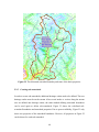
I-99 DEM DATA GENERATION.................................................................. 61
5.4
WATERSHED DELINEATION IN I-99 BASED ON DEM DATA........... 65
5.5
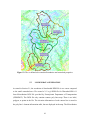
TOPOGRAPHICAL ANALYSIS BASED ON TIN DATA......................... 69
6.0
I-99 ENVIRONMENTAL RESEARCH CASE STUDY................................. 72
6.1
MODEL ASSEMBLY FOR WATERSHED ONE ....................................... 73
6.2
MODEL ASSEMBLY FOR WATERSHED TWO ...................................... 76
vi
6.3
MODELED RAINFALL EVENTS ................................................................ 79
6.4
PARAMETER SELECTION AND MODEL CALIBRATION .................. 83
6.5
PARAMETERS FOR WATERSHED TWO ................................................ 85
6.5.1
Parameters for Watershed Two, Oct 07 2005 Event ........................... 85
6.5.2
Parameters for Watershed Two, Oct 25 2005 Event ........................... 87
6.6
WMS RESULTS FOR WATERSHED TWO ............................................... 87
6.6.1
Watershed Two, Event of Oct 07 2005.................................................. 88
6.6.2
Watershed Two, Event of Oct 25 2005.................................................. 89
6.7
7.0
ANALYSIS OF WMS RESULTS................................................................... 89
HIGHWAY WATERSHED MODEL (HWM) DEVELOPMENT................ 93
7.1
MOTIVATION FOR DEVELOPING HWM ............................................... 93
7.2
WATERSHED DELINEATION .................................................................... 93
7.3
EXCESS RAINFALL GENERATION.......................................................... 95
7.4
SCS AND LE UNIT HYDROGRAPH........................................................... 95
7.5
ISOCHRONE UNIT HYDORGRAPH........................................................ 100
7.5.1
Isochrone curve generation.................................................................. 100
7.5.2
ISO UH derivation ................................................................................ 104
7.6
RUNOFF GENERATION AT EACH SUB-WATERSHED ..................... 105
7.7
CHANNEL AND PIPE ROUTING.............................................................. 105
7.8
RESERVOIR ROUTING.............................................................................. 108
7.9
HYDROGRAPH ADDITION....................................................................... 111
7.10 ROUTING AND ADDING ORDER ............................................................ 112
8.0
APPLICATION OF HWM IN I-99 PROJECT ............................................. 113
8.1
PARAMETERS FOR WATERSHED TWO, ALL EVENTS ................... 113
8.2
HWM RESULTS FOR WATERSHED TWO ............................................ 115
8.3
ANALYSIS OF HWM RESULTS................................................................ 119
8.4
RELATIONSHIP BETWEEN CN AND AMC........................................... 123
8.5
COMPARISON WITH WMS ...................................................................... 130
8.5.1
Three indicators comparison ............................................................... 130
8.5.2
Comparison using parameters............................................................. 131
8.5.3
Comparison using AMC-CN relationship .......................................... 133
vii
8.5.4
9.0
Comments on WMS and HWM software packages .......................... 133
CONCLUSIONS AND RECOMMENDATIONS.......................................... 135
9.1
CONCLUSIONS ............................................................................................ 135
9.2
RECOMMENDATIONS............................................................................... 136
APPENDIX A FORTRAN PROGRAMS FOR EACH MODULE OF HWM ..... 138
PREFACE.................................................................................................................. 139
A.1
HWM.BAT ..................................................................................................... 140
A.2
LINEAR_EXP_UH.F..................................................................................... 141
A.3
EXCESSRAINFALL.F.................................................................................. 143
A.4
HYDRO.F ....................................................................................................... 146
A.5
MUSKINGUM.F............................................................................................ 151
A.6
ADD.F ............................................................................................................. 154
A.7
LEVELPOOL.F ............................................................................................. 159
A.8
KINEMATIC_WAVE.F................................................................................ 164
APPENDIX B USER’S MANUAL OF HWM......................................................... 168
PREFACE.................................................................................................................. 169
B.1
WATERSHED FORMULATION................................................................ 170
B.2
EXCESS RAINFALL GENERATION........................................................ 171
B.3
DIMENSIONLESS UNIT HYDROGRAPH (DUH) GENERATION ...... 172
B.4
SUB-WATERSHED HYDROGRAPH GENERATION............................ 172
B.5
MUSKINGUM ROUTING ........................................................................... 173
B.6
HYDROGRAPH ADDITION....................................................................... 174
B.7
RESERVOIR ROUTING.............................................................................. 175
B.8
KINEMATIC ROUTING ............................................................................. 176
B.9
MASTER FILE .............................................................................................. 177
B.10 HWM EXECUTION ..................................................................................... 177
BIBLIOGRAPHY ......................................................................................................... 179
viii
LIST OF TABLES
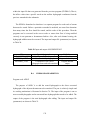
Table 1. Classification of antecedent moisture condition (AMC) .................................... 11
Table 2. The relationship between important model parameters and model results......... 42
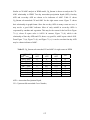
Table 3. Runoff Rainfall Ratio for Each Storm Event in Watershed Two ....................... 85
Table 4. Watershed parameters for Watershed Two, Oct 07 2005 Event......................... 86
Table 5. Routing Parameters for Watershed Two, Oct 07 2005 Event............................. 86
Table 6. CN for each land use for Watershed Two, Oct 07 2005 Event .......................... 86
Table 7. Curve Number for Watershed Two, Oct 25 2005 Event .................................... 87
Table 8. CN for each land use for Watershed Two, Oct 25 2005 Event .......................... 87
Table 9. The comparison of the three criteria in two events for Watershed Two............. 90
Table 10. Coefficients of velocity (ft/s) versus slope (%) relationship for estimating travel
velocities ............................................................................................................ 99
Table 11. The travel time and contributing area for Right_Highway1........................... 101
Table 12. Important parameters used in specific storm events....................................... 114
Table 13. The comparison of the three criteria for Watershed Two............................... 120
Table 14. Up_Stream sub-watershed CN and AMC for eight events in WMS .............. 125
Table 15. Up_Stream sub-watershed CN and AMC for eight events in HWM ............. 127
Table 16. The comparison of the three criteria for Watershed Two with calculated CWV
.......................................................................................................................... 133
Table 17. Input and output of EXCESSRAINFALL.F................................................... 171
Table 18. Input and output of LINEAR_EXP_UH.F ..................................................... 172
Table 19. Input and output of HYDRO.F ....................................................................... 173
Table 20. Input and output of MUSKINGUM.F ............................................................ 174
Table 21. Input and output of ADD.F............................................................................. 175
Table 22. Input and output of LEVELPOOL.F .............................................................. 176
Table 23. Input and output of HYDRO.F ....................................................................... 176
ix
LIST OF FIGURES
Figure 1. Main hydrological processes at a local scale....................................................... 1
Figure 2. Conceptual view of surface runoff .................................................................... 13
Figure 3. Soil Conservation Service synthetic unit hydrograph ....................................... 15
Figure 4. The prism and wedge storage in a channel reach .............................................. 18
Figure 5. Definition sketch for TOPMODEL flow strip................................................... 19
Figure 6. The schematic diagram of the representation of................................................ 21
Figure 7. Initial base-flow recession................................................................................. 24
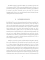
Figure 8. An example of watershed delineation using DEM............................................ 32
Figure 9. An example of watershed delineation using TIN .............................................. 33
Figure 10. Illustration of land use map ............................................................................ 35
Figure 11. Attribute table for land use map ...................................................................... 35
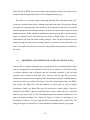
Figure 12. Illustration of soil type map............................................................................. 36
Figure 13. Attribute table for soil type map...................................................................... 36
Figure 14. A mix use of storm total and temporal distribution recording station............. 39
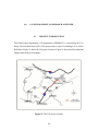
Figure 15. The I-99 project location ................................................................................. 44
Figure 16. The Environmental Impact Study (EIS) area boundary .................................. 45
Figure 17. An illustration of a Parshall flume................................................................... 48
Figure 18. The imported DEM data for LPCW ................................................................ 56
Figure 19. The flow direction of LPCW........................................................................... 57
Figure 20. The stream network of LPCW......................................................................... 58
Figure 21. The converted stream feature arcs in LPCW................................................... 59
Figure 22. The delineated watershed boundary and some of the basin properties ........... 60
Figure 23. The re-defined sub-watershed boundaries and watershed properties.............. 61
Figure 24. The DGN file view in ArcGIS......................................................................... 62
Figure 25. The TIN file view in ArcGIS........................................................................... 63
x
Figure 26. The GRID file view in ArcGIS and WMS ...................................................... 64
Figure 27. The DEM file for I-99 Environmental Research............................................. 66
Figure 28. The DEM file with the flow direction, the stream networks, and stream feature
arcs .................................................................................................................. 66
Figure 29. The automatically generated watershed boundary .......................................... 67
Figure 30. The original DEM file for Watershed SB10-11 .............................................. 68
Figure 31. The DEM file with the flow direction, the stream networks, and stream feature
arcs for Watershed SB10-11 ........................................................................... 68
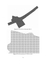
Figure 32. The automatically generated watershed boundary, flats, and pit cells for
Watershed SB10-11 ........................................................................................ 69
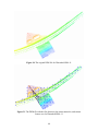
Figure 33. The TIN file for Watershed SB10-11.............................................................. 70
Figure 34. The downstream part of TIN file in detail....................................................... 70
Figure 35. The TIN file with pit cells, flat triangles, and flow direction in Watershed
SB10-11 .......................................................................................................... 71
Figure 36. Schematic layout for Watershed One .............................................................. 73
Figure 37. Elevation - storage - outflow relationship of SB111 ....................................... 75
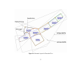
Figure 38. Schematic layout for Watershed Two ............................................................. 77
Figure 39. Elevation - storage - outflow relationship of SB10 ......................................... 78
Figure 40. Elevation - storage - outflow relationship of SB11 ......................................... 79
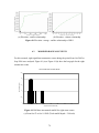
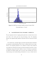
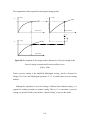
Figure 41. Half hour incremental rainfall for eight storm events ..................................... 79
Figure 42. The rating curve for Ecotones in the two studied watersheds ......................... 88
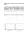
Figure 43. Measured and WMS modeled hydrograph for Oct 07 2005 Event ................. 88
Figure 44. Measured and WMS modeled hydrograph for Oct 25 2005 Event ................. 89
Figure 45. Schematic diagram of Watershed One ............................................................ 94
Figure 46. Schematic diagram of Watershed Two............................................................ 94
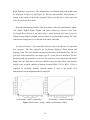
Figure 47. Illustration of different combinations of Tr and Kr .......................................... 97
Figure 48. Illustration of normalized different combinations of Tr and Kr ...................... 97
Figure 49. Illustration of isochrone curve generation..................................................... 101
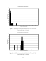
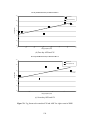
Figure 50. The travel time and contributing area diagram for Right_Highway1 ........... 102
Figure 51. The travel time and contributing area diagram for Right_Highway2 ........... 102
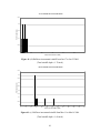
Figure 52. The travel time and contributing area diagram for Right_Highway3 ........... 103
xi
Figure 53. The travel time and contributing area diagram for Right_Highway4 ........... 103
Figure 54. The travel time and contributing area diagram for Up_Stream5................... 103
Figure 55. The travel time and contributing area diagram for Left_Highway6.............. 103
Figure 56. The travel time and contributing area diagram for Down_Stream7.............. 104
Figure 57. Pipe cross section illustration ........................................................................ 107
Figure 58. Development of the storage-outflow function for level pool routing on the
basis of storage-elevation and elevation-outflow curves .............................. 110
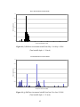
Figure 59. Measured and HWM modeled hydrograph for Oct 07 2005 Event .............. 115
Figure 60. Measured and HWM modeled hydrograph for Oct 25 2005 Event .............. 116
Figure 61. Measured and HWM modeled hydrograph for Nov 27 2005 Event ............. 116
Figure 62. Measured and HWM modeled hydrograph for Jan 17 2006 Event............... 117
Figure 63. Measured and HWM modeled hydrograph for Mar 11 2006 Event ............. 117
Figure 64. Measured and HWM modeled hydrograph for May 11 2006 Event............. 118
Figure 65. Measured and HWM modeled hydrograph for June 26 2006 Event............. 118
Figure 66. Measured and HWM modeled hydrograph for Sept 01 2006 Event ............. 119
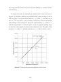
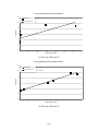
Figure 67. Scatter plot for measured and modeled runoff volume ................................ 121
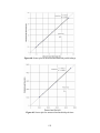
Figure 68. Scatter plot for measured and modeled peak discharge ................................ 122
Figure 69. Scatter plot for measured and modeled peak time......................................... 122
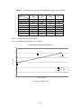
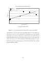
Figure 70. Up_Stream sub-watershed CN and AMC for eight events in WMS............ 126
Figure 71. Up_Stream sub-watershed CN and AMC for eight events in HWM ........... 129
Figure 72. Measured and WMS modeled hydrograph for Oct 07 2005 Event with
calculated CWV ............................................................................................ 132
Figure 73. Measured and WMS modeled hydrograph for Oct 25 2005 Event with
calculated CWV ............................................................................................ 132
xii
LIST OF SYMBOLS
fp
= Infiltration capacity into soil
f∞
= Minimum or ultimate value of f p (at t = ∞ )
fo
= Maximum or initial value of f p (at t = 0 )
t
= Time
K
= Hydraulic conductivity, Muskingum proportionality coefficient,
Coefficient of contraction, flow velocity coefficient.
k
= Recession constant
se
= Initial effective saturation
θe
= Effective porosity
Ψ
=
Wetting front soil suction head
P
=
The incremental precipitation depth, excess rainfall
S
=
The potential maximum retention, watershed slope, watercourse storage
CN
=
The Curve Number
ev
=
Evaporation loss rate
A
=
Watershed area, channel cross section area
ed
=
Evaporation rate
k cov
=
Evaporation conversion factor
V
=
Volume of water
D
=
Water depth
I*
=
Rainfall excess
I
=
Inflow rate
Q
=
Outflow rate
n
=
Manning’s roughness coefficient
xiii
R
=
Hydraulic radius
C
=
Conversion constant, Muskingum coefficient
ai
=
The area draining through a grid square per unit contour length
βi
=
The local surface angle
tan β i
=
The local surface slope
λi
=
Index of hydrological similarity
T0
=
The lateral downslope transmissivity when the soil is just saturated
Si
=
Local storage deficit
m
=
Model parameter controlling the rate of decline of transmissivity with
increasing storage deficit in TOPMODEL
qi
=
The downslope subsurface flow rate per unit contour length
qp
=
Peak discharge
Tp
=
Time of rise
tp
=
Lag time
tr
=
Duration of effective rainfall
Tc
=
Time of concentration
U
=
Unit hydrograph
X
=
Muskingum weighting factor
Tlag
=
The lag time
L
=
Watershed length
g
=
Acceleration of gravity
hi
=
Water pressure head before or after the contraction part
Tr
=
Relative peak time
Kr
=
Recession constant
BS
=
Watershed slope
AOFD
=
Average overflow distance
MSL
=
Maximum stream length
MSS
=
Maximum stream slope
NSTPS
=
The number of integer steps for the Muskingum routing
APD
=
Antecedent precipitation depth
xiv
R
=
Pipe radius, the recharge rate in TOPMODEL
ck
=
Kinematic wave celerity
θ
=
The wetted angle in pipe flow
E
=
Specific energy
B
=
Flume width
CWV
=
The channel water velocity
xv
ACKNOWLEDGEMENTS
I would especially like to thank my advisor, Dr. Rafael G. Quimpo, for his constant
support and guidance throughout the duration of my Ph.D. study. I would also like to give
special thanks to Dr. Ronald D. Neufeld, Dr. Jeen-Shang Lin, Dr. William Harbert, and
Dr. Xu Liang for their mentorship in my graduate work. Special gratitude is extended to
colleagues and staff in the Department of Civil and Environmental Engineering for their
invaluable support and assistance provided throughout my study.
I would also express gratitude to my parents and younger sister for their consistent
support from my family. Thanks are also given to all my friends who have helped me in
my study and research.
xvi
1.0
1.1
INTRODUCTION
BACKGROUND
Hydrology is the scientific study of water and its properties, distribution, and effects on
the earth’s surface, soil, and atmosphere (McCuen 1997). Water circulation in the air,
land surface and underground constitutes hydrologic cycle. The cycle has no beginning or
end. Hydrology researchers are often faced with problems of runoff prediction,
contaminant concentrations, water stages, etc. Due to the great spatial and temporal
variability of watershed characteristics, precipitation patterns, contaminant transport rules,
and the number of variables involved in the physical processes, rainfall-runoff
relationship is one of the most complex hydrologic phenomena. Prediction of
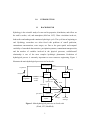
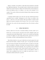
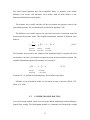
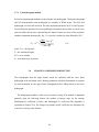
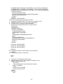
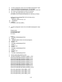
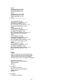
hydrological process is extremely important to water resources engineering. Figure 1
illustrates the main hydrological processes at a local scale.
Precipitation
evaporation
evaporation
evaporation
Land
surface
transpiration
Vegetation
stemflow
through
rainfall
Water
body
overland flow
capillary rise
flood
infiltration
interflow
Soil
percolation
capillary rise
Groundwater
aquifer
Stream
channel
baseflow
recharge
watershed
discharge
Figure 1. Main hydrological processes at a local scale
(Ward, 1975, Modified)
1
In recent years, in many places of the world, the processes of rapid population growth,
highway construction, urbanization, and industrialization have increased the demand for
clean water. Simultaneously, these processes also greatly change the hydrological
conditions and have negative influences on storm water quantity and quality. For water
quantity, urbanization increases the percentage of impervious area in a watershed, thus
the surface runoff in a post-development area becomes greater than in that in predevelopment area. Consequently, the base flow and interflow in post-development area is
significantly reduced. Furthermore, the discharge flow time pattern changes, i.e. the peak
discharge increases and peak time become shorter.
Besides quantity, water quality is affected by a combination of natural and human
factors. Natural factors affecting water quality include precipitation intensity and amount,
geology, soil types, topography and vegetation cover, etc. Meybeck et al. (1989) provided
a detailed review of this topic. Most of these factors can be, and have been, affected by
humans; for example, changes in river discharge due to construction, abstraction,
urbanisation or impounding; discharges from industry, agriculture or sewerage, etc
(Meybeck M, et al. 1989).
To protect communities from adverse environmental disturbance, the evaluation of
the influence of urbanization or construction is urgently needed for the corresponding
watershed areas.
1.2
PROBLEMS STATEMENT
The Pennsylvania Department of Transportation (PENNDOT) is constructing the U.S.
Route 220/I-99/State Route (S.R.) 6220 project that is a part of a large effort to extend I99 to I-80 at Bellefonte. Highway construction is often the cause of substantial adverse
environmental effects, both during the construction phase and during the operational
phase. To appraise the environmental influence of highway construction, monitoring and
evaluating the effectiveness of various mitigation techniques implemented are being done
during the construction of I-99 to enable improved management of corridor resources.
2
The research also includes developing enhanced capabilities to predict impacts and
identifying suitable mitigation measures for future highway constructions.
The research includes four parts. The first part is the evaluation of approved erosion
and sediment controls to determine best management practice. Intimately tied to the first
part is the prediction of the runoff as a result of the rainfall on the construction project.
This is the second part of the project. The third part is to monitor and assess the wetland
hydro-biological indicators for land use planning in the highway. The last part is to
evaluate the effectiveness and sustainability of stream restoration, rehabilitation, and
relocation projects as part of mitigation for road construction. This study focuses on the
second part.
1.3
OBJECTIVE AND SCOPE
The objective of this research is to build a runoff prediction model using GIS techniques
for a watershed affected by highway construction. The model will be designed to predict
runoff at several outlets in the watershed based on rainfall, land use, soil type, detention
pond location, stream distribution, water velocity, and basin slope, etc. For efficiency and
cost effectiveness, runoff prediction method and local applicability will be verified. A
successful model can reduce expensive monitoring instrumentation and personnel
training cost in future projects.
The scope of this research will involve numerical computer simulations and field data
collection, assimilation and analysis. A GIS-based rainfall-runoff model will be
developed using the Watershed Modeling System (WMS) platform and calibrated to
simulate the hydrology and hydraulics phenomena along the stream system draining the
selected constructed basin near I-99 highway. To compensate for the shortcomings the
WMS model, a new model -- Highway Watershed Model (HWM) is developed. The
results from WMS and HWM will be analyzed and compared. The relationship between
antecedent moisture condition (AMC) and curve number (CN) will be investigated.
3
Highway watershed is more difficult to model than natural mountainous watersheds
due to high human disturbance. The watershed elevation is altered by human construction
and hence the stream directions are changed. The alteration makes elevation changes too
mild (on the highway surface, for example) or too steep (at the mountain cut, for
example). This research will discuss the methods dealing with these human interventions
in the watershed.
In applying GIS-based model, some GIS source data and watershed characteristics
requirements must be available. Unfortunately, not all of them are available to this
project. A trade-off to deal with GIS-based model and traditional conceptual model
applied in the practical watershed will be discussed. This is also a reason to develop
HWM model. Also, surface flow data and ground flow data will be collected to calibrate
the model.
1.4
LITERATURE REVIEW
Extensive studies have been done on watershed modeling. Generally, models can be
divided into two broad categories: physically based model (distributed model) and
conceptually based models (lumped model). A recent review on rainfall-runoff modeling
is given by O’Loughlin et al. (1996). Singh (1988) provides a general survey of most of
the techniques available for modeling hydrological systems at that time.
Physical-based models are one type of models that are based on physical laws and
known initial and boundary conditions. Presently, quite a few physically based models
have been developed and applied. Physically-based models are normally run with point
values of precipitation, evaporation, soil moisture and watershed characters as primary
input data and produce the runoff hydrographs. They are generally accurate, but difficult
to use. Many of the assumptions in these models cannot be satisfied in practice. Users
must determine a huge number of parameters, which are often difficult to obtain. In
regions where precipitation data series are available but runoff data are scarce, a
deterministic rainfall-runoff model is a good tool.
4
Kavvas et al. (2004) presented a new model Watershed Environmental Hydrology
Model (WEHY) to the modeling of hydrologic processes in order to account for the effect
of heterogeneity within natural watersheds. The parameters of the WEHY are related to
the physical properties of the watershed, and they can be estimated from readily available
information on topography, soils and vegetation/land cover conditions (Chen et al.
2004a). The parameters can be obtained from GIS database of a watershed without
resorting to a fitting exercise. The model was applied to the Shinbara-Dam watershed and
has produced promising runoff prediction results (Chen et al. 2004b).
Liang (2003) presented two improvements on the three-layer variable infiltration
capacity (VIC-3L) model, which is also originally developed by Liang. The VIC model is
a macro-scale hydrologic model that solves full water and energy balances. It can be
applied to various watershed sizes ranging from small watersheds to continental and
global scale. One improvement of the research is to include the infiltration excess runoff
generation mechanism in the VIC model by considering effects of spatial sub-grid soil
heterogeneities on surface runoff and soil moisture simulations. The other is to consider
the effects of surface and groundwater interaction on soil moisture, evapotranspiration,
and recharge rate. The two improvements are tested by comparing the modelled total
runoff and groundwater table with observed values at the watershed of Little Pine Creek,
Etna, Pennsylvania. Results show that the new version of VIC simulates the total runoff
and groundwater table very well.
To investigate the influence of urban pavement and traffic on runoff water quantity,
Cristina et al. (2003) developed a kinematic wave model which accurately captured the
significant aspects of typical urban runoff. The impacts of the paved urban surface and
traffic were examined with respect to the temporal distribution of storm water runoff
quantity. The kinematic wave theory gave predictions of the time of concentration that
were more accurate than other more common methods currently in use.
5
Campling et al. (2002) developed TOPMODEL, a semi-distributed, topographically
based hydrological model, and applied it to continuously simulate the runoff hydrograph
of a medium-sized (379km2), humid tropical catchment. The researcher found that water
tables were not paralle to the surface topography. To increase the weighting of local
storage deficits in upland areas, a reference topographic index λREF was introduced into
the TOPMODEL structure. Not confined in deterministic modeling, this research also
assessed the performance of the model with randomly selected parameter sets and set
simulation confidence limits by using generalized likelihood uncertainty estimation
(GLUE) framework. The model simulated the fast subsurface and overland flow events
superimposed on the seasonal rise and fall of the base-flow very well. It was also found
that there was increased uncertainty in the simulation of storm events during the early and
late phase of the season.
Conceptual-based lumped models are well known for their simplicity. They are also
applied widely by many researchers. Fontaine (1995) evaluated the accuracy of rainfallrunoff model simulations by using the 100-year flood of July, 1, 1978 on the Kickapoo
River, in southwest Wisconsin as a case study. The accuracy of a simple analysis is
compared to that of an elaborate, labor-intensive analysis. The more elaborate modeling
approach produces more accurate results. Fontaine concluded that the error in the
precipitation data used for calibrating the model appears to be the primary source of
uncertainty.
Lidén (2000) did an analysis of conceptual rainfall-runoff modeling performance in
different climates. It was found that the magnitude of the water balance components had
a significant influence on model performance. Beighley (2002) presented a method for
quantifying spatially and temporally distributed land use data to determine the degree of
urbanization that occurs during a gauge’s period of record. Madsen (2002) presented and
compared three different automated methods for calibration of rainfall-runoff models.
Besides building mathematical models, researchers have developed object-oriented
software to model rainfall-runoff relationship. Garrote et al. (1997) presented a software
6
environment for real-time flood forecasting using distributed models. The system, Realtime Interactive Basin Simulator (RIBS), provides an object-oriented framework for
implementation of a class of distributed rainfall-runoff models satisfying certain formal
requirements. RIBS manages process organization and data handling; facilitation of user
interaction and result visualization and provision of access to model structure, hydrologic
processes, and model inference.
Other widely used packaged software include Watershed Modeling System (WMS,
developed by Environmental Modeling Research Laboratory, Brigham Young
University), Storm Water Management Model [SWMM, developed by U. S.
Environmental Protection Agency (EPA)], Hydrologic Engineering Center Hydrological
Modeling System (HEC-HMS, developed by U. S. Army Corps of Engineering) and
Hydrological Simulation Program -- FORTRAN (HSPF, developed by U. S. EPA).
1.5
LAYOUT OF THIS DISSERTATION
The dissertation is organized as follows. Chapter Two contains basic theories on
watershed modeling; both physical-based and conceptual-based model theories. Chapter
Three reviews the procedures for developing the GIS-based model -- WMS model, which
the author investigated in detail but found to be inadequate. Chapter Four gives an
overview of the studied watershed. Chapter Five illustrates some difficulties in the model
building. Chapter Six presents a case study on the selected watershed and the modeling
results. Chapter Seven develops the new model -- Highway Watershed Model (HWM),
an alternative to the WMS model. Chapter Eight gives the modeling results of HWM; it
also analyzes and compares the results from WMS and HWM. The last chapter gives the
conclusions of this research and recommendations to future study.
7
2.0
THEORY AND METHODOLOGY
For many years, hydrologists have attempted to understand the transformation of
precipitation to runoff, in order to forecast stream flow for purposes such as water supply,
flood control, irrigation, drainage, water quality, power generation, recreation, and fish
and wildlife propagation.
Since the 1930s, numerous rainfall-runoff models have been developed to simulate
hydrologic cycle. As shown schematically in Figure 1, water precipitates from cloud to
land surface; water evaporates from the land surface to become part of atmosphere.
Precipitation may be intercepted by vegetation, become overland flow on the ground
surface, infiltrate into the ground, flow through the soil as sub-surface flow and discharge
into streams as surface runoff. Some of the intercepted water and surface runoff returns to
the atmosphere through evaporation. The infiltrated water may percolate deeper to
recharge groundwater. Groundwater may rise near to the land surface through capillary or
be evaporated through vegetation root.
A watershed is a region of land where water drains down slope into a specified body
of water, such as a river, lake, ocean or wetland. A watershed includes both the waterway
and the land that drains to it. A watershed boundary is determined by its topographic
characteristics. Ridges, hills and mountains often play the role of delineating a watershed
from other watersheds.
Based on the description above, the main hydrological processes can be modelled by
the following four modules. Each module can be simulated by several methods. This
proposal considers only some representatives of each module.
1. Precipitation loss module;
8
2. Surface water flow module;
3. Channel flow module;
4. Base flow module;
2.1
PRECIPITATION LOSS MODELING
Rainfall-runoff model computes runoff volume by computing the volume of water that is
intercepted, infiltrated, stored, evaporated, transpired and subtracted from the
precipitation. The loss can be broadly categorized into infiltration (down loss) and
evaporation (up loss).
Infiltration from watershed area can be computed by the Horton Equation, GreenAmpt model and the Soil Conservation Service (SCS) curve number (CN) method (SCS,
1972).
The Horton model is based on empirical observations showing that infiltration
decreases exponentially from an initial maximum rate to some minimum rate over the
course of a long rainfall event. The model describes the infiltration capacity as a function
of time as:
f p = f ∞ + ( f o − f ∞ ) ⋅ e − kt
(2.1)
where:
f p = infiltration capacity into soil, mm/hr,
f ∞ = minimum or ultimate value of f p (at t = 0), mm/hr,
f 0 = maximum or initial value of f p (at t = 0), mm/hr,
t = time from beginning of storm, hr,
k = decay coefficient, hr-1.
9
This equation describes the exponential decay of infiltration capacity evident during
heavy storms. Required parameters are f 0 , f ∞ and k. The actual values of f 0 , f ∞ and k
depend on the soil, vegetation, and initial moisture content. These parameters can be
estimated using results from field infiltration-meter tests for a number of sites of the
watershed and for a number of antecedent wetness conditions. If it is not possible to use
field data to find estimates of f 0 , f ∞ and k, the guidelines given by the U.S.
Environmental Protection Agency can be used (Huber et al, 1988).
The Green-Ampt equation (Green et al, 1911) for infiltration rate is
⎛ ψ ⋅ Δθ ⎞
f (t ) = K ⎜⎜
+ 1⎟⎟
F
(
t
)
⎝
⎠
(2.2)
F(t) is the cumulated infiltration and can be expressed as
⎛ F (t )
⎞
+ 1⎟⎟
F (t ) = K ⋅ t + ψ ⋅ Δθ ln⎜⎜
⎝ ψ ⋅ Δθ
⎠
(2.3)
where Δθ = (1 − se ) ⋅ θ e ;
se = initial effective saturation, dimensionless, 0 ≤ se ≤ 1;
θ e = effective porosity, dimensionless, 0 ≤ se ≤ 1;
K = hydraulic conductivity, m/hr;
t = infiltration time, hr;
Ψ = wetting front soil suction head, cm;
The cumulated infiltration can be calculated by successive substitution using Equation
2.3. The infiltration parameters are given by Rawls et al (1983).
The Soil Conservation Service (SCS) curve numbers (CN) describe the surface’s
potential for generating runoff as a function of the soil type and land use on surface.
Curve numbers range between 0 < CN ≤ 100, with 0 as the theoretic lower limit
describing a surface that absorbs all precipitation, and 100 the upper limit describing an
impervious surface such as asphalt, or water, where all precipitation becomes runoff. The
10
method computes the excess precipitation (Pe) generated for an incremental depth of
precipitation falling on an area using the following relationship
Pe =
( P − 0.2S ) 2
( P + 0.8S )
(2.4)
where P = the incremental precipitation depth, inch;
S = the potential maximum retention, inch.
The value S is related to the curve number by
S=
1000
− 10
CN
(2.5)
where CN = the Curve Number, which is defined by SCS.
Equation 2.4 applies only for P ≥ 0.2S, otherwise all the precipitation is assumed lost to
infiltration. The normal antecedent moisture conditions (AMC II) CN value is defined
and tabulated by SCS based on different soil type and land use. For dry conditions (AMC
I) or wet conditions (AMC III), equivalent curve numbers can be computed by
and
CN ( I ) =
4.2CN ( II )
10 − 0.058CN ( II )
(2.6)
CN ( III ) =
23CN ( II )
10 + 0.13CN ( II )
(2.7)
As a result, the SCS method provides the depth of excess precipitation resulting from a
given depth of precipitation falling over an area during a specific time interval. The range
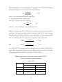
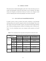
of antecedent moisture conditions for each class is shown in Table 1.
Table 1. Classification of antecedent moisture condition (AMC)
for the SCS method of rainfall abstractions
(SCS, 1972)
AMC Group
Total 5-day antecedent rainfall (inch)
Dormant season
Growing season
I
Less than 0.5
Less than 1.4
II
0.5 to 1.1
1.4 to 2.1
III
Over 1.1
Over 2.1
11
In this research, SCS abstraction method is employed to obtain excess rainfall, which is
used to generate hydrograph in later procedures. As we can see from above discussion,
several parameters are needed in Horton model, such as, minimum or ultimate
infiltration f ∞ , maximum or initial infiltration rate f 0 , and decay coefficient k. More
parameters are needed in Green-Ampt equation. These parameters are not available. In
contrast, the only parameter in SCS CN method is the curve number, which can be found
in National Engineering Handbook (SCS, 1972) based on soil type and land use. The land
use and soil type are relatively easy to determine. The environmental research is
performed according to PennDOT’s need. PennDOT requires a pragmatic model, which
they can operate, transfer to other projects, or make revision after the model has been
built. Thus, SCS CN method is selected according to project’s practical situation.
Evaporation is considered as a loss “of the top.” That is, evaporation is subtracted
from rainfall depths prior to calculating infiltration. Thus, subsequent use of the symbol i
for “rainfall intensity” is really rainfall intensity minus evaporation rate. The loss rate is
computed by
ev = A ⋅ ed / k cov
(2.8)
where:
ev = evaporation loss rate, ft3/day,
A = surface area at the water level in the unit, ft2,
ed = evaporation rate, inch/day, and
k cov = evaporation conversion factor.
The values of ed should be supplied for each interval of the simulation period.
2.2
DISTRIBUTED SURFACE WATER MODELING
The distributed surface water modeling is based on differential equations that allow the
flow rate and water level to be computed as functions of space and time, rather than of
12
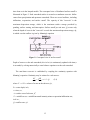
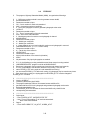
time alone as in the lumped models. The conceptual view of distributed surface runoff is
illustrated in Figure 2. Each watershed surface is treated as a nonlinear reservoir. Inflow
comes from precipitation and upstream watersheds. There are several outflows, including
infiltration, evaporation, and surface runoff. The capacity of this "reservoir" is the
maximum depression storage, which is the maximum surface storage provided by
ponding, surface wetting, and interception. Surface runoff per unit area, Q, occurs only
when the depth of water in the "reservoir" exceeds the maximum depression storage, dp,
in which case the outflow is given by Manning's equation.
Figure 2. Conceptual view of surface runoff
Depth of water over the sub-watershed (d in inches) is continuously updated with time (t
in seconds) by solving numerically a water balance equation over the sub-watershed.
The non-linear reservoir is established by coupling the continuity equation with
Manning’s equation. Continuity may be written for a sub-area as:
dV
dD
=A
= A ⋅ i * −Q
dt
dt
(2.9)
where V = A ⋅ D = volume of water on the sub-area, ft3,
D = water depth, inch,
t = time, sec,
A = surface area of sub-area, ft2,
i * = rainfall excess = rainfall/snowmelt intensity minus evaporation/infiltration rate,
inch/sec,
Q = outflow rate, cfs.
13
The outflow is generated using Manning’s equation
Q=
1
⋅ D ⋅ R 2 / 3 ⋅ S 1/ 2
n
(2.10)
where
n = manning’s roughness coefficient,
D = depth of depression storage, ft,
R = hydraulic radius, R = Area / WetPerimeter , ft
S = sub-watershed slope, ft/ft.
Equations (2.9) and (2.10) may be combined into one non-linear differential equation that
may be solved for one unknown, the depth, d. This produces the non-linear reservoir
equation
dD
1
= i * − ⋅ R 2 / 3 ⋅ S 1/ 2
dt
n
(2.11)
Equation (2.11) is solved at each time step by means of a simple finite difference scheme
(Huber et al, 1988).
2.3
LUMPED SURFACE WATER MODELING
The lumped surface water modeling is accomplished by the unit hydrograph method. The
unit hydrograph of a watershed is defined as a hydrograph resulting from one inch
spatially-uniform excess rainfall over the watershed at a constant rate for an effective
duration. Several types of unit hydrographs, such as Snyder unit hydrograph, Clark unit
hydrograph, SCS dimensionless unit hydrograph, have been developed.
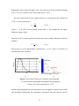
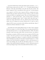
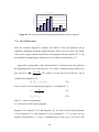
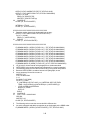
The SCS dimensionless hydrograph is a synthetic unit hydrograph in which the
discharge is expressed as a ratio of q to peak discharge qp and the time as the ratio of time
t to the time of rise of the unit hydrograph, Tp. Figure 3 (a) shows the SCS dimensionless
hydrograph. The values of qp and Tp may be estimated using a model of a triangular unit
14
hydrograph, which is shown in Figure 3 (b), where the time is in hours and the discharge
in m3/s.cm or cfs/in (Source: Soil Conservation Service, 1972).
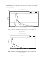
The Soil Conservation Service suggests the time of recession may be estimated as
1.67Tp. qp can be expressed as
qp =
CA
Tp
(2.12)
where C = 2.08 (483.4 in the English system) and A = the drainage area in square
kilometers (square miles).
The time of rise Tp can be expressed in terms of lag time tp and the duration of effective
rainfall tr.
tr
+tp
2
Tp =
(2.13)
The lag time tp can be approximately calculated by t p ≅ 0.6Tc , where Tc is the time of
concentration of the watershed.
1
q/q(peak)
0.8
0.6
0.4
0.2
0
0
0.5
1
1.5
2
2.5
3
3.5
4
4.5
5
t/Tp
(a)
(b)
Figure 3. Soil Conservation Service synthetic unit hydrograph
(a) Dimensionless hydrograph (b) triangular unit hydrograph
(Source: Soil Conservation Service, 1972)
Once the unit hydrograph has been determined, it may be applied to find the direct runoff
and streamflow hydrograph. For calculation convenience, the time interval used in
15
defining the excess rainfall hyetograph ordinates should be the same as that for which the
unit hydrograph was specified. The discrete convolution equation
Qn =
n≤ M
∑P
m =1
m
⋅ U n −m +1
(2.14)
can be used to yield the direct overland runoff hydrograph,
where P = The excess rainfall;
U = The unit hydrograph;
n = The nth time interval (recording runoff and unit hydrograph);
m = The mth time interval (recording rainfall);
M = The total number of time interval (recording runoff);
2.4
DISTRIBUTED CHANNEL ROUTING
Similar to surface water distributed model, the distributed channel flow model is based on
partial differential equations (the Saint-Venant equations for one-dimensional flow) that
allow the flow rate and water level to be computed as functions of space and time. They
describe the passage of a flood wave down a section of reach both in space and time. On
the contrary, the lumped model does not use the Saint-Venant equations and only
considers time factor for solutions.
The Saint-Venant equations include the continuity equation and momentum equation.
In complete form, the Saint Venant equations are (Chow et al, 1988)
Continuity equation:
Momentum equation:
∂Q ∂A
+
=0
∂x ∂t
(2.15a)
∂y
1 ∂Q 1 ∂ ⎛ Q 2 ⎞
⎟⎟ + g − g (S 0 − S f ) = 0
⋅
+ ⋅ ⋅ ⎜⎜
A ∂t A ∂x ⎝ A ⎠
∂x
Local
Convective
Pressure Gravity
Friction
acceleration
acceleration
force
force
force
term
term
term
term
term
16
(2.15b)
The Saint Venant equations have three simplified forms, i.e. dynamic wave model,
diffusion wave model, and kinematic wave model. Each of them defines a onedimensional distributed routing model.
The dynamic wave model considers all the acceleration and pressure terms in the
momentum equation. The accounted terms are labeled in Equation 2.15b.
The diffusion wave model neglects the local and convective acceleration terms but
incorporates the pressure terms. The simplified momentum equation of diffusion wave
model is
∂y
− g
∂x
g
(S
0
− S
f
)=
Pressure
Gravity
Friction
force term
force term
force term
(2.16)
0
The kinematic wave model is the simplest of the distributed model. It neglects the local
acceleration, convective acceleration and pressure terms in the momentum equation. The
simplified momentum equation of kinematic wave model is
g
(S
− S
0
f
)=
0
Gravity
Friction
force term
force term
(2.17)
It assumes S0 = Sf and the friction and gravity forces balance each other.
Solutions to the distributed model can be found in many references (Fread 1973,
Chow et al. 1988).
2.5
LUMPED CHANNEL ROUTING
Level pool routing method, linear reservoir model and the Muskingum method belong to
lumped flow routing. The Muskingum method is a commonly used hydrologic routing
17
method for handling a variable discharge-storage relationship. The model considers two
components of storage, wedge and prism. During the advance of a flood wave, inflow
exceeds outflow, producing a wedge of storage. During the recession, outflow exceeds
inflow, resulting in a negative wedge. The prism is formed by a volume of constant cross
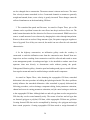
section along the length of prismatic channel. Figure 4 shows the prism and wedge
storage in a channel reach.
Figure 4. The prism and wedge storage in a channel reach
(Chow et al, 1988)
The total storage is the sum of two components
S = KQ + KX(I-Q)
(2.18a)
which can be rearranged to be the storage function
S = K[XI + (1 - X)Q]
(2.18b)
Equation 2.16b represents a linear model for routing flow in streams.
The channel outflow is expressed as
Qj+1 = C1Ij+1 + C2Ij + C3Qj
(2.19)
where C1, C2, C3 are Muskingum coefficient and defined as
C1 =
Δt − 2 KX
2 K (1 − X ) + Δt
(2.20a)
C2 =
Δt + 2 KX
2 K (1 − X ) + Δt
(2.20b)
C3 =
2 K (1 − X ) − Δt
2 K (1 − X ) + Δt
(2.20c)
18
2.6
TOPOGRAPHICALLY BASED BASE-FLOW MODELING
In areas that have much vegetation or consist of sandy soils, base-flow becomes
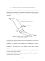
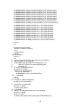
important in total water balance. The representative topographical based base-flow model
is TOPMODEL (Beven, 1995). Figure 5 illustrate the term definitions of TOPMODEL in
a flow strip.
Ai = Total area drained in flow strip
ai = area drained per unit contour length = A/w
tanβi =local surface slope
βi
dxi
wi = contour length
Figure 5. Definition sketch for TOPMODEL flow strip
(Kirkby, 1997, Modified)
TOPMODEL uses four basic assumptions to relate local downslope flow from a point to
discharge at the watershed outlet.
Assumption 1: The dynamics of the saturated zone are approximated by successive
steady state representations.
Assumption 2: The recharge rate r (m/h) entering the water table is spatially
homogeneous.
Assumption 3: The effective hydraulic gradient of the saturated zone is approximated by
the local surface topographic gradient β.
Assumption 4: The distribution of downslope transmissivity T0 (m2/h) with depth is an
exponential function of storage deficit.
19
TOPMODEL uses the distribution of the topographic index as an index of
hydrological similarity, which indicates the propensity of landscape areas to become wet.
⎛ a
⎞
λi = ln⎜⎜ i ⎟⎟
⎝ tan β i ⎠
(2.21)
where ai = the area draining through a grid square per unit contour length;
tan β i = the local surface slope;
Under assumption 1 and assumption 2, the downslope subsurface flow rate per unit
contour length qi (m2/h) is:
qi = rai
(2.22)
where r = the recharge rate;
Under assumption 3 and assumption 4, qi (m2/h) is also:
q i = T0 e − Si / m tan β i
(2.23)
where T0 = the lateral downslope transmissivity when the soil is just saturated;
Si = local storage deficit;
m = model parameter controlling the rate of decline of transmissivity with increasing
storage deficit.
By combining Equation (2.22) and Equation (2.23), the local soil moisture deficit Si can
be derived:
⎛ rai
S i = −m ln⎜⎜
⎝ T0 tan β i
⎞
⎟⎟
⎠
(2.24)
The mean watershed storage deficit S is obtained by integrating Equation (2.24) over the
entire area Ai of the watershed:
S=
⎛
rai
1
Ai ⎜⎜ − m ⋅ ln
∑
A i
T0 ⋅ tan β i
⎝
⎞
⎟⎟
⎠
where Ai = the fractional area of the topographic index class i.
20
(2.25)
Assuming that the water table recharge and the soil transmissivity are spatially constant,
then ln r and ln T0 are eliminated from Equation (2.25) and Si is expressed as:
⎛
ai
S i = S + m ⋅ ⎜⎜ λ − ln
tan β i
⎝
⎞
⎟⎟
⎠
(2.26)
where λ is the areal average of the topographic index:
A
⎛ a
1
λ = ⋅ ∫ ln⎜⎜ i
A 0 ⎝ tan β i
⎞
⎟⎟ ⋅ Ai ⋅ dA
⎠
(2.27)
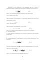
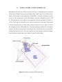
At each topographic index class λi , unsaturated and saturated zone fluxes are modeled.
Figure 6 shows the schematic diagram of the representation of the local storage deficit, Si,
for different topographic indices.
⎛ a
⎞
λi = ln⎜⎜ i ⎟⎟
⎝ tan βi ⎠
Un-saturated aquifer
Un-saturated aquifer
Saturated aquifer
Saturated aquifer
⎛
a ⎞
Si = S + m ⋅ ⎜⎜ λ − ln i ⎟⎟
tan βi ⎠
⎝
S
Aquifuge
Aquifuge
Un-saturated aquifer
Saturated aquifer
Figure 6. The schematic diagram of the representation of
the local storage deficit for different topographic indices
(Campling, 2002, Modified)
The vertical drainage qv from the unsaturated store at any point i is controlled by the local
saturated zone deficit Di, which depends on the depth of the local water table (Beven and
Wood, 1983):
qv =
S uz
Di ⋅ t d
(2.28)
21
where Suz = the storage in the unsaturated zone;
td = time delay constant that introduces longer residence times to cater for deep water
table levels.
The watershed flux of water entering the water table, Qv is calculated by assuming the qv
of each topographic index class:
Qv = ∑ qv Ai
(2.29)
i
Output from the saturated store is represented by the base-flow term, Qb, which can be
calculated using a subsurface storage deficit-discharge function of the form:
Qb = Q0 ⋅ e − S / m
(2.30)
where Q0 = A ⋅ e − λ is the discharge when S is zero.
The watershed average deficit S is updated by subtracting the unsaturated zone recharge
and adding the base-flow from the previous time step:
S t = S t −1 + [Qbt −1 − Qvt −1 ]
(2.31)
The initial base-flow Q0 and the initial root zone storage deficit Sr0 are input at the start of
the modeling.
Experience in modeling the Booro-Borotou watershed in the Cote d’Ivoire (Quinn,
1991), and watersheds in the Prades mountains of Cataluna, Spain, suggests that
TOPMODEL will only provide satisfactory simulations once the watershed has wetted up.
In many watersheds that tend to receive precipitation in short, high intensity storm, or
receive low precipitation, the soil seldom reach a “wetted” state, and the response may be
controlled by the connectivity of any saturated downslope flows. Short, high intensity
storm may lead to the production of infiltration excess overland flow, which is not
usually included in TOPMODEL. The watersheds in I-99 Environmental Research often
receive such kind of rainfall. Some assumptions are violated in the studied watershed, so
the TOPMODEL is not used in the studied watershed.
22
Another reason not to use TOPMODEL is that many parameters are difficult to obtain
in I-99 Project. For example, one of the key parameters in TOPMODEL is the index of
hydrological similarity λi of each grid square, which depends on the area drained per unit
contour length ai and the local surface slope tan β i . To determine λi of each grid square,
ai and tan β i of each grid square are needed. This includes tremendous calculation,
which is not practical for I-99 Project.
2.7
SIMPLER LUMPED BASED-FLOW MODELING
A simpler lumped model -- the exponential recession model, is available to describe the
base-flow. The recession model has been used to explain the drainage from natural
storage in a watershed (Linsley et al, 1982). It defines the relationship of Qt , the base
flow at anytime t , to an initial value as:
Qt = Q0 k t
(2.32)
where:
Q0 = initial base-flow (at time zero),
k = recession constant.
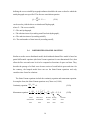
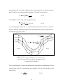
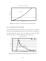
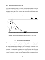
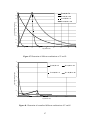
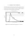
The base-flow is illustrated in Figure 7. The shaded region represents base-flow in this
figure; the contribution decays exponentially from the starting flow. The total flow is the
sum of the base-flow and the direct surface runoff.
23
Figure 7. Initial base-flow recession
k is defined as the ratio of the base-flow at time t to the base-flow one day earlier. The
starting base-flow value Q0 is an initial condition of the model. It may be specified as a
flow rate (ft3/s), or it may be specified as a flow per unit area (ft3/s/mile2).
2.8
GIS-BASED WATERSHED MODELING
With the development of computer science, hydrological models have been combined
with Geographic Information System (GIS) technology. GIS is a special type of
information system in which the data source is a database of spatially distributed features
and procedures to collect, store, retrieve, analyze, and display geographic data. In other
words, a key element of the information used by utilities is its location relative to other
geographic features and objects (Shami, 2002). It combines spatial locations with their
corresponding various information.
GIS is a class of concepts instead of one product. There are many kinds of GIS data,
which are supported by different software packages. They may not be compatible with
each other. Shape files represent city, park and airport using point feature. They represent
road, river and pipe using polylines features. They also represent watershed, lake and
country using polygon features. This is not always the case. In large scale, for example, a
24
city or an airport is often represented by polygons. A feature object comprises an entity
with a geographic location, typically describable by points, arcs, or polygons.
On the contrary, Grid files represent everything using equal dimensional pixels. In a
certain scale map, a large object is represented using more pixels; while a small object is
represented using fewer pixels.
Digital Elevation Models (DEM) are regular grid data structures that contain twodimensional arrays of elevations where the spacing between elevations is constant in the
x and y directions. In this manner, it is like a grid file. The resolutions of DEM are
normally 30 × 30 square meters or 90 × 90 square meters.
Triangulated Irregular Networks (TIN) is another type of digital elevation map. A
TIN is built from a series of irregularly spaced points with elevations that describe the
surface at that point. In contrast to DEM, the elevation points are irregularly distributed.
From these points, a network of linked triangles is constructed. Adjacent triangles,
sharing two nodes and an edge, connect each other to form a surface. A height can be
calculated for any point on the surface by interpolating a value from the nodes of nearby
triangles. In addition, each triangle face has a specific slope and aspect. TIN can be used
for visualization, as background elevation maps for generating new TIN or DEM, or
perform basin delineation and drainage analysis.
A TIN file is flexible in representing different variation terrain. If a watershed
elevation varies too much in a small area, more points are needed for accuracy purpose.
However, if a watershed elevation is very flat in a large area, fewer points can be used to
save storage space. On the contrary, DEM always represents a watershed using identicalsized square pixels.
In essence, a raster file representing elevation is similar to DEM and Grid. A raster
file is also a regular grid data structure that contains a two-dimensional array of
elevations. However, since raster files, grid files and DEM files are developed by
25
different agencies, they are processed digitally differently. Vector files represent objects
similar to shape files. Vector files may also represent rivers using polyline features and
represent watersheds using polygon features. However, vector files and shape files are
processed digitally computer differently.
Shape files, grid files, Triangulated Irregular Network (TIN) and Digital Elevation
Model (DEM) files are supported by ArcGIS (Environmental Systems Research Institute,
1999). DEM files, Raster files and Vector files are supported by IDRISI (Eastman, 1999).
DEM files, shape file and another type of TIN files are supported by Watershed
Modeling System (Environmental Modeling Research Laboratory, Brigham Young
University, 1999). TIN files used in WMS are incompatible with TIN files used in
ArcGIS. DEM files used in ArcGIS are realized through grid files and are incompatible
with DEM files used in IDRISI and WMS.
GIS-based hydrological models utilize readily available digital geospatial information
more expediently and more accurately than manual-input methods. Also, the
development of basic watershed information will help the user to estimate hydrologic
parameters. After obtaining adequate experience in GIS-generated parameters, users can
make parameter estimation more efficiently. GIS-based hydrological models may use
different GIS data as different layers. To make different GIS data display and work in the
correct location, coincident spatial referencing is needed for different layers.
HEC-GeoHMS was developed by U.S. Army Corps of Engineers, Hydrological
Engineering Center (U. S. Army Corps of Engineers, Hydrologic Engineering Center,
2003). HEC-GeoHMS links GIS tool (ArcView3.2) and hydrologic model (Hydrologic
Modeling System - HMS). HEC-GeoHMS combines the functionality of ArcInfo
programs into a package that is easy to use with a specialized interface. With the
ArcView capability and the graphical user interface, the user can access customized
menus, tools and buttons instead of the command line interface in ArcInfo. The
hydrologic algorithms in the model are the same as HEC-HMS. First, HEC-GeoHMS
imports DEM data and fills sinks in the data. Second, it generates flow direction and
26
streams based on DEM data. Then the following procedure is to delineate watershed and
sub-watershed boundaries. The newly generated files are stored in separate layers. The
pertinent watershed characteristics can be extracted from the source DEM data and the
generated stream and boundary data. After these processes, a HEC-HMS schematic map
and project can be exported. Other parameters, such as meteorological, routing and
infiltration parameters, need to be set before the project runs. In fact, HEC-GeoHMS
prepares the input file and schematic map for HEC-HMS. By using GIS data, detailed
watershed characteristics are obtained automatically for the HEC-HMS model. However,
the source GIS files, such as DEM file, are not generally available and difficult to
generate from the beginning.
Quimpo et al. (2003) develop a quasi-distributed GIS-based hydrologic model (QDGISHydro). The model consists of several separate modules, which process data
describing the spatial variation of watershed properties, and compute the runoff time
series at the watershed outlet. Data processing and visualization is handled primarily by
GIS software IDRISI32, while self-written computer programs perform the bulk of the
computations. The model is designed to operate as simply and generally as possible,
requiring only four external data sets as input (DEM, land coverage, soil coverage, and
incremental precipitation depths) to create all other data needed to compute the direct
runoff for the watershed under study. The model is able to deal with non-uniform excess
rainfall for each watershed pixel. Land use and soil type files are available for most of
United State watersheds. Incremental precipitation depth files can be created by the user
easily. Unfortunately, DEM file is not always available and the model can only process
DEM file as source elevation information. Users cannot build a research model without
source DEM file.
WMS was developed by Environmental Modeling Research Laboratory of Brigham
Young University. It is flexible in creating a practical model using various input source
data, or even creating a model from the scratch. WMS is able to use Shape file, ArcInfo
Grid file, DEM or TIN source data to create watershed delineation. In case of none of the
source file is available, users can import aerial photographs or even scanned watershed
27
maps as referenced spatial data. Although some GIS characteristics are missing in this
case, users are able to build a flexible, practical model for watersheds where source data
are not adequate. GIS data such as land use and soil type files can be created by the user
or imported from readily available data. These techniques greatly enhance the
applicability of WMS in watershed modeling and make WMS not only a research
package, but a pragmatic tool in watershed modeling project.
Another GIS environmental modeling package is Better Assessment Science
Integrating Point and Non-point Sources (BASINS). BASINS was developed by the U. S.
Environmental Protection Agency (EPA). It takes advantage of developments in software
and data management technologies and uses the ArcView3.X as the integrating
framework to provide the user with a comprehensive watershed management tool. In this
manner, it is like HECGEOHMS. However, BASINS focus on point and non-point
pollutant modeling instead of watershed modeling.
28
3.0
GIS-BASED HYDROLOGICAL MODEL - WMS APPROACH
As discussed in Chapter Two, WMS is flexible in creating a practical model using
various input source data, or even creating a model from the beginning without any
topological GIS data. It may also be used for dealing with constructed watersheds. In this
environmental impact of highway assessment research, WMS was tested because it has
many desirable features. This chapter will discuss the features of WMS model. The
author has devoted a lot of effort in examing whether it is suitable for the project.
3.1
WMS INTRODUCTION
WMS provides a platform for using various models, such as HEC-1, National Flood
Frequency Program (NFF), HEC-RAS (River Analysis System), Hydrological Simulation
Program - FORTRAN (HSPF), and CE-Qual-W2, etc. Each model is designed for
particular purpose. HEC-1 was developed by The Hydrologic Engineering Center (HEC),
U.S. Army Corps of Engineering. It performs flood hydrograph computations associated
with a single recorded or hypothetical storm. The main purpose in Task B of I-99 project
is to model the surface water in the construction site watershed. Therefore, model HEC-1
in the WMS package is mainly employed in this research.
3.2
COORDINATE SYSTEM SETTING AND CONVERSION
A digital image is very important in building WMS model. An image consists of a
collection of pixels, each of which has its own value. The resolution of the pixel
29
determines the area and detail represented in the image. Images in WMS are used to
derive data such as pipes, streams, confluences, land use, and soil type files, etc. It also
provides a background map to the watershed. In order to use the image to represent
proper length, area and orientation, the user must geo-reference the image. Georeferencing an image defines x and y coordinates so that distances, areas and orientations
computed from the image are correct.
To geo-reference the image correctly, users need to know the coordinates of two or
three points on the image. The coordinates can be the Universal Transverse Mercator
(UTM) system, the geographic system, state plane or the local system. Once the
coordinate of two or three points are determined, all other points in the map can be
determined according to the relative position of these points. Different coordinate
systems can be converted to each other if necessary. Geo-referencing is extremely
important if multiple function layers are imported to represent the same region. In this
situation, correct geo-referencing guarantees the coincidence of the same points, lines and
polygons in the different layers.
3.3
SOURCE DATA IMPORTING AND CREATING
Digital Elevation Models (DEM) is a commonly used digital elevation source and an
important part of using WMS for watershed characterization. Many agencies provide
DEM data. These include the Meteorological Resource Center (http://www.webgis.com),
U.S. Geology Survey (http://gisdata.usgs.net), GeoCommunity/GIS Data Depot
(http://www.gisdatadepot.com),
Pennsylvania
Spatial
Data
Access
(http://www.pasda.psu.edu), etc. Triangulated Irregular Networks (TIN) is another type
of digital elevation map. TIN can be used for visualization, as background elevation maps
for generating new TIN or DEM, or perform basin delineation and drainage analysis in
WMS.
30
After DEM or TIN files are imported into WMS, users can modify the elevation value
of a certain point in WMS. TIN files are not widely published on the web. Therefore, it is
more difficult to find the proper TIN file than DEM file. Fortunately, TIN and DEM can
be converted to each other. Theoretically, users can also create TIN file from the
beginning manually. However, since watershed normally consists of thousands of points,
creating TIN files from scratch is not realistic.
3.4
WATERSHED DELINEATION
Both DEM and TIN are used as elevation information files to delineate a watershed. First,
flow directions for individual DEM cells or TIN vertices are created. By creating an
outlet on a down stream branch, stream network and watershed boundary are generated
based on flow direction and stream threshold. After the watershed is delineated, the
basin’s characters, such as area, basin’s slope, maximum flow distance, etc., can be
calculated automatically by WMS. If the user is not satisfied with the automatically
generated streams or watershed boundaries, he can add streams and outlet manually. Also,
users are free to combine adjacent sub-watersheds into one and divide a big subwatershed into several. However, all operations must have solid practical basis instead of
only imagination. An example of watershed delineation using DEM and TIN file is
shown in Figure 8 and Figure 9, respectively.
Although it is convenient to generate watershed delineation using DEM or TIN files,
there are some limitations. In a real watershed, there may be some spikes or pits. A spike
is a cell whose elevation is higher than the surrounding cells. A pit is a cell whose
elevation is lower than the surrounding cells. Flat terrains, flat channels also exist in
reality. While a spike is generally not a serious problem in hydrologic analysis, a pit or
flat element on the other hand can be. This can be problematic because the water flows
into the pit and never flows out. Thus, the flow path is discontinued. The model cannot
determine the flow direction if flat terrains are encountered. In order to perform any type
of hydrologic analysis, pits and flat elements must be removed. WMS program has tools
31
to remove a small amount of error elements by changing their values through
interpolation.
However, these tools are only useful when a few errors happen. If huge numbers of
pits, flat terrains congregate together to form a big pond, their elevation values cannot be
altered though interpolation. Thus, they cannot be removed easily. Actually, they should
NOT be altered if they form a big pond. Once they are altered, the model can not reflect
the real watershed characteristics. While pits and flat terrains are very common in reality,
WMS cannot deal with it very well. Sometimes, users need to find out other methods to
solve this problem.
Figure 8. An example of watershed delineation using DEM
32
Figure 9. An example of watershed delineation using TIN
3.5
DRAINAGE COMPONENT EDITING
As stated above, automatic delineation is not enough even for identifying a watershed.
Some model components must be edited manually.
Streams can be generated automatically or drawn by users. Automatic streams are
generated from DEM or TIN files. If the automatically generated streams are not enough,
users need to draw the stream manually. Streams are abstracted to be polylines in WMS.
Several types of polylines are employed in WMS model. They are generic, stream, pipe,
lake and ridge. After drawing a polyline using draw line tool, user must assign it to be
stream type. The drawing direction of a stream must from downstream to upstream. Other
types of lines also should be assigned to proper line type.
The basins boundaries are polygon-shaped. Polygons are categorized into the
following types: generic, lake, reservoir and drainage boundary. Polygons cannot be
33
drawn directly in WMS. User needs to draw a closed polyline, assign it to be generic line,
and then build a polygon and assign it to be a drainage boundary type.
The outlet is a conceptual point connecting upstream flow and downstream flow.
Points are categorized into generic, drainage outlet and route point. The point type should
be assigned to a drainage outlet. One outlet must be accompanied with a basin to form the
correct watershed model schematic structure. A reservoir works as water storage or flood
detention structure in the watershed. Although an actual reservoir has a certain area and
shape, its function can be abstracted into an outlet in WMS model. The reservoir’s
characteristics are input into outlet routing strategies. Thus, an outlet contains not only
channel routing, but also reservoir routing strategies. A reservoir is not required in every
outlet. If an outlet does not have a reservoir, only channel routing method is defined for
the outlet.
3.6
IMPORTING AND CREATING OF LAND USE AND SOIL DATA
Land use file is a polygon schematic map overlapped onto the watershed boundary. It has
land use data properties and is defined in Land Use Layer. Similarly, soil data file is also
a polygon schematic map overlapped onto the watershed boundary. It has soil data
properties and is defined in Soil Data Layer. Land use and soil type files are used to
calculate the composite curve number of sub-watershed. Most publicly available land use
and soil data files are in Shape file format. First, users should import them into WMS;
then connect the Shape files with their database to obtain land use and soil digital
information. Finally, the Shape files must be converted to feature objects, which are
actually used in WMS. Land use is classified into 20 types, while soil type is classified
into four types by SCS (1972). The relationship between curve number and land use, soil
type is described in Chapter Two. Figure 10, Figure 11, Figure 12, and Figure 13 are
illustrations of land use, soil type map and their corresponding tables, respectively. The
polygons in Figure 10 and Figure 12 represent different land use and soil type patches.
34
Figure 10. Illustration of land use map
Figure 11. Attribute table for land use map
35
Figure 12. Illustration of soil type map
Figure 13. Attribute table for soil type map
36
The rectangular area inside is the un-delineated watershed DEM file. Normally, the
coverage area of the land use and soil type file is much bigger than studied watershed.
If land use and soil type files are not available, the user can create them manually.
First, the user must create land use and soil type coverages in WMS separately. For each
type of coverage, land use and soil type polygons are created using polygon creating
method described in Section 3.5. After creating polygons, a database table regarding land
use and soil type must be filled to connect the digital information with the polygon spatial
area. The database table works the same way as a database when Shape format soil and
land use file are available.
3.7
WATERSHED INFORMATION AND CALCULATION METHOD
The watershed information required for modeling in WMS include four main groups.
3.7.1
Basin data
Basin data contain the basin’s elementary characteristics. The basin’s name identifies it
from other basins. A descriptive name is helpful in building and running the model. The
basin’s area is always calculated by WMS if the geo-referencing information is correct. If
the basin’s area is incorrect, user should modify the geo-reference information instead of
changing area directly. If a hydrograph is known for a given basin, there is no need to
compute a synthetic hydrograph. This hydrograph can be input by defining the
hydrograph using the XY Series Editor. The XY Series Editor is a general purpose editor
for entering curves or pairs of lists of data. If the user wants to optimize the modeled
hydrograph using an observed hydrograph, the observed hydrograph can be input also
using XY Series Editor.
37
3.7.2
Precipitation
Several options of precipitation can be defined. One commonly used precipitation method
is basin average precipitation. With this method, a time distribution can be entered via the
XY Series Editor. Several standard storm distributions can be loaded automatically from
this editor. The standard storm distributions often can not satisfy the user’s requirement.
In this case, distributions can be created by the user directly. An average precipitation is
also input to account for total rainfall.
The basin average method is convenient in small watersheds, where the rainfall can
be regarded as spatially uniform. However, rainfall is normally spatially non-uniform in
large watersheds, where multiple rain gages are used. A gage may be a storm total and/or
temporal distribution recording station type. Recording stations allow for a continuous
rainfall accumulation to be entered. The storm total station only allows for a single
rainfall value for the event. Figure 14 shows a mix use of storm total and temporal
distribution recording station. Gage_A and Gage_B are temporal distribution recording
stations, which are "imaginary" gages and do not participate building the Thiessen
network, which is used in building the rain gage coverage polygons. Gage1 to Gage 10
are storm total stations and they compose a Thiessen network. The temporal distribution
of Gage1 to Gage10 is determined by nearest recording station.
38
Figure 14. A mix use of storm total and temporal distribution recording station
3.7.3 Loss method
WMS provides several options in loss method modeling. The uniform loss method is the
simplest method. It uses an initial value and a uniform value to define infiltration losses.
The Horton loss method uses the starting value of the loss coefficient and the exponential
factor as the main parameters. The Green-Ampt method employs initial effective
saturation, effective porosity, hydraulic conductivity and wetting front soil suction head
to compute infiltration rate and accumulative infiltration. SCS curve number loss method
is used in this research. These methods are described in detail in Chapter Two.
39
3.7.4
Unit hydrograph method
Several unit hydrograph methods, such as Snyder unit hydrograph, Clark unit hydrograph
and SCS dimensionless unit hydrograph are available in WMS model. The SCS unit
hydrograph is used in this research. The most important parameter in SCS is the lag time.
Several different equations have been published to determine the lag time of a basin. User
also can define the lag time equation himself. Many of them use some of the geometric
attributes computed automatically. Eq. 3.1 is used to calculate lag time defined by SCS.
TLag
1000
[(
− 10) + 1]0.7
= L0.8 × CN
1900 × S
(3.1)
where TLag = the lag time;
L = the watershed length;
CN = curve number;
S = watershed slope in percent.
3.8
CHANNEL AND RESERVOIR ROUTING
The hydrographs from the upper basins would be combined with the lower basin
hydrograph at the watershed outlet. Routing parameters should be determined to compute
lag and attenuation on the upper basin hydrographs before adding them to the lower
hydrograph.
The Muskingum method is often used in channel routing. The method is dependent
primarily upon the following factors: the number of integer steps for the routing,
Muskingum K coefficient in hours and Muskingum X coefficient. The algorithm is
explained in Chapter Two. The integer step number and K coefficient are determined by
water flow velocity in the channel.
40
A reservoir is placed at an outlet to model water storage and retention. Although the
reservoir does not occupy area in the model, its characteristics can be defined using a
table. The important reservoir routing data are elevation-discharge relationship,
elevation-storage relationship and initial condition. Using these data, reservoir routing
can be performed without knowing reservoir’s area.
3.9
JOB CONTROL SETTING
Most of the parameters required for HEC-1 model are defined for basins, outlets and
reservoirs. However, there are some global parameters that control the overall simulation
and are not specific to any basin or reach in the channel. These parameters are defined in
WMS job control module.
A model’s title, ID, author and short description can be filled in the first part. Then,
the modeling event starting date and calculation unit should be filled. The most important
data here are the computational interval and the number of hydrograph ordinates. They
determine how long the resulting hydrograph should be displayed. If the display time is
too short, the hydrograph will not be shown completely. If the display time is too long,
the hydrograph shown is to rough and many details are missed. Proper computational
interval and the number of hydrograph ordinates are needed to get good modeling results.
They can be estimated by observing similar outflow records.
As stated in 3.7.1, the user has the option to optimize unit hydrograph and loss rate
parameters in the modeling so the calculated hydrograph will match the observed
hydrograph. User also can optimize routing parameters using observed inflow and
outflow hydrographs and a pattern lateral inflow hydrograph for the routing reach. They
are also set in job control module.
41
3.10
DISPLAY OUTPUT
The model results are detailed hydrographs at each outlet. At the outlet where reservoir is
located, both hydrographs flowing into and flowing out can be displayed. The display
formats can be diagram, text format, Excel format, etc. For direct view, a diagram is often
used. For comparing with an observed hydrograph, Excel format is often used.
3.11
EVALUATION OF PARAMETER INFLUENCE
No model is perfect. In order to evaluate if the model is satisfactory, several important
modeling characteristics should be compared with the observed hydrograph. They are the
total volume of the runoff, the number of peaks, each peak time and each peak discharge
value. Different modeling parameters influence the modeling results in different ways.
Table 2 lists the relationship between some important model parameters and model
results.
Table 2. The relationship between important model parameters and model results
Influences
Parameters
CN
Slope
Basin
Area
Precipitation
Watershed
Length
Water
Routing
Velocity
No. of Steps
K
Initial
Reservoir
Elevation
Storage
Increase Parameters (Decrease - Opposite Influences)
Total Volume
Peak Time
Peak Discharge
Increase
No Change
Increase
Increase
Early
Increase
Increase
No Change
Increase
Increase
No Change
Increase
Decrease
Later
Decrease
Increase
Early
Increase
Decrease
Decrease
Increase
Later
Later
Early or No
Change
Later
Decrease
Decrease
Increase
No Change
42
Decrease
It is strange that the number of peaks of the discharge seldom changes with the above
parameters. Actually, the number of peaks of the discharge is mostly controlled by
precipitation pattern, i.e. the number of peaks and distribution of the precipitation. After
surface flow and channel routing, the number of peaks of the discharge will be fewer than
the number of peaks of the precipitation. However, large peaks in precipitation separated
by long time intervals will be reflected in the peaks of the discharge.
The above table indicates the parameters and model results in one single subwatershed. Generally, the hydrograph comes from several sub-watersheds, outlets and
reservoirs, which have several sets of parameters. In this case, the model results are more
complicated to anticipate.
43
4.0
I-99 ENVIRONMENTAL RESEARCH OVERVIEW
4.1
PROJECT INTRODUCTION
The Pennsylvania Department of Transportation (PENNDOT) is constructing the U.S.
Route 220/I-99/State Route (S.R.) 6220 project that is a part of extending I-99 to I-80 at
Bellefonte. Figure 15 shows the I-99 project location. Figure 16 shows the Environmental
Impact Study (EIS) area boundary.
Figure 15. The I-99 project location
44
Figure 16. The Environmental Impact Study (EIS) area boundary
45
Highway construction often causes substantial adverse environmental effects, both during
and after construction. Construction-induced impacts include soil erosion resulting from
clearing, grubbing and earth movement and rainfall runoff. Relocation of streams, direct
and indirect impacts to wetlands, and encountering hazardous wastes are also the
construction environmental impacts. Highway constructions may also unintentionally
damage site of archeological and culture significance. During the operation phase,
highways affect the environment through the introduction of pollutants in storm water
runoff, permanent changes in land use and resulting ecological consequences.
The objective of the I-99 environmental research is to monitor and evaluate the
effectiveness of various mitigation techniques implemented during the highway
construction to provide an improved management of the highway, and to develop
enhanced capabilities to predict impacts and identify suitable mitigation measures for
future highway projects in Pennsylvania (Quimpo, 2004). The project will provide
immediate benefits in helping to minimize the construction and operational impacts of I99. It will provide long term benefits by developing Best Management Practices (BMPs)
for Pennsylvania highways, and through the development of models that can be used
throughout Pennsylvania to predict construction impacts and mitigation success. These
models will provide for greater accuracy and reliability in future designs, while reducing
the cost of expensive field and laboratory investigations.
4.2
4.2.1
PROJECT COMPONENTS
Task A: Evaluation of erosion and sediment controls
As stated in Chapter One, this environmental research includes four tasks. The primary
focus of Task A is to continue the research on Best Management Practices (BMPs). The
key issue for this task is to conduct field reconnaissance, monitoring of field sites under
46
normal and high rainfall, and assess the results in a final report. The research includes the
following work:
1. Periodic site visits with professional observations, reporting and digital pictures.
2. Digital photographs will be taken and logged with narrative. Digital pictures will be
stored electronically to be retrieved as needed for study and comparison, incorporated
into a GIS database, and incorporated into the final project report. GIS mapping will be
linked to a database including modeling results and to digital photographs.
3. The field crew will identify selected samples that to be analyzed for turbidity analysis,
trace heavy metals and filtered COD. Field measurements of pH and temperature will be
taken. Such studies provide new insight into the behavior of BMPs subjected to runoff
containing residuals typical of motorized vehicle traffic.
4. A qualitative risk-based evaluation method will be prepared. The evaluation aims at
the relative environmental impacts associated with the ineffectiveness or failure of the
BMPs on downstream receiving waters, including wetlands and streams. The method will
address modes, likelihood, and consequences of failure, and will consider reliability,
longevity, costs, environmental benefits and liability.
4.2.2
Task B: Hydrologic monitoring and modeling
Task B is the prediction of the quantity of runoff on the complex construction project.
The primary focus of Task B is to perform monitoring and modeling to evaluate the
hydrologic regime associated with the highway cut area, the down slope wetlands, and
the mechanism used to maintain groundwater flow to the wetlands, i.e. infiltration
galleries. The model, which is to be calibrated using the field monitoring data, will be
used to evaluate, explain and predict the effectiveness of the infiltration galleries in
maintaining groundwater flow to the down slope wetlands. The objective is to develop a
model that can be applied at the I-99 project to reliably predict future hydrologic impacts
to the wetlands and thereby reduce costly monitoring efforts. The model may then be
used in the design of other projects with similar conditions. Runoff prediction techniques,
for the specific local construction site, will be built and verified. To reduce expensive
47
monitoring instrumentation at other projects, the model should be portable, which means
the procedures can be used at other construction sites with adjustments for site-specificity.
The portability requirement is an important criterion in the selection and choice of model.
As part of the monitoring effort included in Task B, water level recorders were
installed at several locations. The recorders are classified into three categories. The first
category, which is called Well Logger, is used to record the ground water table changes.
The second category, Deep Ecotone, is used to record the sub-surface flow in the down
stream watershed. The last category, Shallow Ecotone, is employed to obtain water depth
in the watershed outflow flume. Ecotone is the brand of the instruments. The Shallow
Ecotone instrument is a Parshall flume. Figure 17 is an illustration of a Parshall flume,
which has a contraction in the middle.
Figure 17. An illustration of a Parshall flume
When water flows through the flume, the contraction forces the water flow from subcritical status to critical flow status. At the critical depth, the specific energy is minimized
and discharge is uniquely related to the water depth. Equation (4.1) shows the specific
energy expression.
E = h+
Q2
2gA 2
(4.1)
where:
E = specific energy,
h = water depth,
Q = discharge,
48
A = cross section area,
g = gravity acceleration.
To get the minimum of E, Equation (4.1) is differentiated and assigned to be zero.
dE
Q2B
= 1−
=0
dh
gA3
(4.2)
where:
B = flume width.
Equation (4.2) can be solved by substituting flow velocity V = Q/A and water depth h =
A/B.
dE
V2
= 1−
=0
dh
gh
(4.3)
Then the flow velocity and discharge can be calculated by
V = gh
(4.4)
Q = B ⋅ g ⋅ h3
(4.5)
Theoretically, the discharge can be calculated from depth directly. In practice, the
relationship of water depth and discharge is calibrated and provided by manufacturer.
Once the relationship between water depth and discharge is determined, we do not need
to get discharge from the instrument. Instead, we get water depths and convert them into
outflow discharges in the hydrological analysis using the relationship. The Well Logger,
Deep Ecotone and Shallow Ecotone instruments automatically record water levels at sixhour intervals, one-hour intervals and one-hour intervals, respectively. The data will be
used in Task B for calibrating the model and evaluating model prediction results, and in
task C for assessing wetland conditions and key wetland indicators. The locations of
monitoring instruments for Watershed One and Watershed Two are illustrated in Figure
36 and Figure 38, respectively.
The Environmental Impact Study (EIS) is about 10 miles long and 1 mile wide.
Because the EIS area does not belong to one watershed, it is divided into several sections.
49
Along the highway, length marks are coded from 0 to 535. One unit mark’s distance
interval is 100 ft. Hydrological modeling is performed in the selected two watersheds,
which are at about the length mark of 185 and 400. For purposes of Task A, ponds were
constructed downstream of the highway at several locations. The corresponding ponds in
the two watersheds are SB111 (around length mark 400) and SB10, SB11 (around length
mark 185). These two watersheds were selected because PENNDOT constructed special
underground filter galleries in the watersheds. Also, Ecotones were installed at these two
watersheds’ outlets. As stated above, one of the objectives of this project part is to reduce
instrumentation and data collecting expenses. Due to high cost of buying and installing
the instruments, only the two test watersheds have Ecotone recorders. The model built on
these two watersheds will be applied to other watersheds with some site specific
modifications.
A key feature of this highway watershed design is the inclusion of infiltration
galleries under the roadway which catch intercepted groundwater from areas upslope.
Runoff from newly impervious surfaces resulting from construction would be collected
and routed to storm water management ponds. This slows down runoff production
through reduced transport rate and also improves its quality through detention in the
ponds, catching the first flush.
Runoff from undisturbed land is channeled directly to receiving streams as clean
water. This is achieved by routing the clean runoff directly to downstream outlet without
passing the intermediate watersheds. A rain gage was installed in Port Matilda, a town
near the watersheds. Because the watershed is not too large, only one rain gage was used.
The location of rain gage is illustrated in Figure 16.
The model focuses on the hydrologic phenomenon of a system designed to
incorporate an infiltration stratum under the roadway. This project presents a unique
opportunity to test the new concept in design to minimize adverse impacts on the
environment, particularly with respect to hydrologic regimes in highway cut areas. The
uniqueness lies in the minimum disruption of the hydrologic regimes prior to construction.
50
4.2.3
Task C: Monitoring and assessment of wetland hydro-biological indicator
Task C will focus on the wetlands down slope of the cut areas in Section C10 (Figure 16),
and mitigation wetlands. The environmental document compiled for the project through
the National Environmental Policy Act (NEPA) process will be utilized to provide the
initial baseline documentation of resources in the project area. A GIS database will be
compiled of project corridor wetlands. Data will be organized to provide a clear
illustration of each wetland’s position in the landscape based upon watershed,
topographic setting, and relationship to the new highway and other anticipated land use
changes. The database will include information concerning those features that may
influence function and value. These data includes wetland type, topographic setting and
geologic conditions, hydrologic regime, soil type, adjacent land uses and soil types,
dominant vegetation species, habitat value, water quality issues, and uniqueness.
Photographs of each wetland, wetland delineation data forms, and other relevant
supporting information will be linked to this database.
Each monitoring wetland will be subject to periodic field surveys to assess parameters
affecting function and value. The following parameters will be monitored at the
frequencies listed.
1.
2.
3.
4.
5.
Water chemistry;
Hydrologic conditions;
Vegetation community;
Birds;
Amphibians and reptiles;
6. Mammals;
7. Benthic macro-invertebrates;
8. Soil chemistry;
9. Soil condition;
10. Adjacent land use and including dominant
vegetation community
The initial survey on the selected wetlands will include collection of data on the
various animal classifications identified to provide a broad spectrum of baseline data on
the community composition and population levels. The subsequent field monitoring will
focus on the benthic macro-invertebrates and amphibians, which are key bio-indicator
groups.
51
An overall assessment of function and value will be completed for each monitored
wetland for pre and post-construction conditions, and for post-construction mitigation
wetlands in accordance with the appropriate methodology. These results will then be
analyzed utilizing multiple linear regression, ordination techniques, or other appropriate,
ecologically-valid statistical analyses to determine the relative importance of the
monitored parameters in explaining observed changes in functions and values, by wetland
type and setting, over time.
The results of the previous efforts will be synthesized to provide a regional
framework for predicting construction impacts on wetlands by type and setting based on
key indicators. An important component of these analyses will be the development of a
regional model that will predict the impact of construction on wetland species diversity,
relative abundance of domain classification, and the performance of uncommon or unique
species. This model will be developed for use as a tool in assessing impacts of future
highway projects utilizing key indicators and standardized measures of diversity.
4.2.4
Task D: Evaluation of stream restoration, rehabilitation and relocation
The objective of Task D is to assess the effectiveness of stream restoration, stabilization,
and relocation practices for highway construction and their ability to sustain a complex,
ecologically diverse healthy stream system over the long term. Highway constructions
often impact streams directly and indirectly. These construction projects typically require
some type of mitigation, which includes stream bank stabilization, stream relocation,
stream restoration, and possibly mitigation elsewhere to compensate for impacts of the
project.
52
5.0
DIFFICULTIES IN MODEL BUILDING
5.1 DIFFICULTIES STATEMENT
This research focuses on Task B, the prediction of runoff on the complex construction
site. Hydrological modeling is performed in the selected two watersheds, which are
approximately at about the stations of 400 (SB111, Watershed One) and 185 (SB10,
SB11, Watershed Two) in the construction project’s alignment. Due to the following
features, this construction watershed is difficult to model.
1. The watershed areas are very small. The area of Watershed One is about 0.085 sq
mile (54.40 acres). The area of Watershed Two is about 0.072 sq mile (46.08 acres).
Although DEM files are available online, they cover large areas, normally in 10 to 100 sq
miles. The resolution of the DEM is 30 × 30 sq meters. The studied watersheds are only a
few points in this kind of DEM file. Detailed watershed delineation cannot be performed
in such coarse DEM files. Since DEM files are coarse, the converted TIN files also
cannot be used. The same problems exist in the downloaded land use and soil type files.
Land use and soil type files are even in larger scale, usually in 100 to 1000 sq miles. If
the online land use and soil type files are used, probably the whole watershed falls in only
one type of soil and land use.
2. The watershed geomorphological characteristics and land uses have been changed
recently by construction. The online data do not reflect the updated elevation and land
use changes. For example, during or after the construction, land use in the watershed land
use changes from uncultivated land or forest to paved highway. Streams are created or
covered. Stream flow directions are changed. Elevations, hence the water flow channel,
53
are also changed due to construction. The nature stream is sinuous and coarse. The water
flow velocity in nature watershed is slow. Constructed channels or streams are generally
straight and smooth; hence, water velocity is greatly increased. These changes cannot be
reflected simultaneous on the downloading GIS data.
3. The watershed has ponds and flat areas. As stated in Chapter Three, pits or flat
elements can be a problem because the water flows into the pit and never flows out. The
model cannot determine the flow direction if a flat area is encountered. WMS has tools to
remove a small amount of error elements by changing their values through interpolation.
However, these tools are useless if huge amount of pits, flat points congregate together to
form a big pond. Even if they are removed, the model can not reflect the real watershed
characteristics.
4. In the highway construction, an infiltration gallery under the roadway is
constructed to catch the infiltration water from the construction area. Runoff from new
impervious surfaces resulting from construction would be collected and routed to storm
water management ponds. An underground pipe is also installed to conduct water from
upstream clean area directly to downstream outlet without passing the ponds.
Underground filtration gallery, detention pond and underground pipe are much different
from regular stream and must be modeled using a suitable model component.
As stated in Chapter Three, after obtaining the topographic GIS data, watershed
delineation is the next procedure in building the hydrological model. The above problems
mainly influence the watershed delineation. After watershed is properly delineated, the
following procedures, such as drainage component editing, basin parameters estimation,
channel and reservoir routing parameters estimation, and job control setting are irrelevant
to the topographic GIS data. Although land use and soil type data are also categorized as
GIS data, they can be created manually easily. The reason is land use and soil type data
are featured (polygon or polyline) GIS data, while topographic GIS data are grid data.
Creating featured GIS data can be accomplished by drawing a few polygons and assign
them certain properties. Creating topographic GIS data needs to assign thousands of
54
pixels different values. This cannot be accomplished manually. The main difficulty in the
model is the availability and accuracy of topographic GIS data.
5.2
WATERSHED DELINEATION FOR A LARGE NATURAL WATERSHED
To illustrate the procedure of delineating a large natural watershed, Little Pine Creek
Watershed (LPCW) is employed here. LPCW covers about 15.02 km2 (5.8 mile2) and is
located mostly with Shaler and O’Hara Townships in north central Allegheny County,
Pittsburgh, Pennsylvania. LPCW was selected because it contains no significant detention
pond or other storage. Little Pine Creek is a tributary of Pine Creek, which flows into the
Allegheny River at the town of Etna. The DEM data files were obtained from
Pennsylvania Spatial Data Access (PASDA) website.
5.2.1
Importing DEM data
DEM data should be imported into WMS. The imported DEM data is shown in Figure 18.
55
Figure 18. The imported DEM data for LPCW
5.2.2
Computing flow direction
The flow direction should be computed in WMS. The flow direction form a network of
streams on top of the DEM. WMS computes flow direction for individual DEM cells and
creates streams based on these directions. Figure 19 shows a flow direction of LPCW.
Figure 20 shows a stream network of LPCW.
56
Figure 19. The flow direction of LPCW
57
Figure 20. The stream network of LPCW
5.2.3
Determining the outlet point and stream feature arcs
The outlet point is determined according to project need. Theoretically, it can be any
point in the watershed. In this example, a point in the stream near the lower left corner is
selected. By choosing a point on a lower stream branch, a watershed outlet is defined.
WMS then uses the flow direction and accumulation data from Section 5.2.2 to convert
the streams network into stream feature arcs. Figure 21 is the converted stream feature
arcs in LPCW.
58
Figure 21. The converted stream feature arcs in LPCW
5.2.4
Defining the watershed boundary
The stream feature arcs can be used to define the basin boundaries. Because the DEM
contains elevation data, the model can be used to calculate the basin properties such as
watershed area, slope, and average overflow distance, etc. It is not just a schematic of the
watershed. Figure 22 show the delineated watershed boundary and some of the basin
properties,
where A = watershed area;
BS = watershed slope;
AOFD = average overflow distance;
L = watershed length;
MSL = maximum stream length;
MSS = maximum stream slope;
59
Figure 22. The delineated watershed boundary and some of the basin properties
5.2.5
Creating sub-watersheds
In order to create sub-watersheds, additional drainage outlets need to be defined. The new
drainage outlets must be on the stream. After several nodes or vertices along the stream
arcs are defined into drainage outlets, the same method defining watershed boundaries
can be used again to define sub-watersheds. Figure 23 shows the re-defined subwatershed boundaries and watershed properties. Due to space availability, Figure 23 only
shows two properties of the watershed boundaries. However, all properties in Figure 22
can be shown for each sub-watershed.
60
Figure 23. The re-defined sub-watershed boundaries and watershed properties
5.3
I-99 DEM DATA GENERATION
As stated in Section 5.1, the resolution of downloaded DEM file is too coarse compared
to the small watershed area. We created a 2×2 sq ft DEM file for Watershed SB10-11
from MicroStation DGN file provided by Pennsylvania Department of Transportation
(PENNDOT). The DGN file only contains contour poly lines map. There is no label,
polygon, or points in the file. The elevation information of each contour line is stored in
the poly line’s element information table, but not displayed in the map. The MicroStation
61
DGN format contour line file can be converted into DEM file through the following
procedures.
1. DGN file is imported into ArcGIS using Add Data function. The DGN file is shown in
Figure 24.
Figure 24. The DGN file view in ArcGIS
2. DGN file is converted into TIN file in 3D Analyst, an extension of ArcGIS. The
function to be used is Create TIN From Features… The TIN file is shown as in Figure 25.
62
Figure 25. The TIN file view in ArcGIS
3. TIN file is converted into GRID file in 3D Analyst using the function of TIN To
Raster… Resolution of the GRID file can be assigned in this procedure. For example, we
can assign it as 2×2 sq ft or 5×5 sq ft. The GRID file is shown as in Figure 26.
63
Figure 26. The GRID file view in ArcGIS and WMS
4. Start WMS, turn to the GIS module, enable the ArcObject function, add ArcGIS GRID
file into WMS using Add Data function. The GRID file appearance in WMS is the same.
It is also shown in Figure 26.
5. The GRID file is converted into DEM format using Convert To DEM function. The
DEM file is shown in Figure 27.
After DEM file is obtained, the watershed delineation can be performed in WMS.
This is illustrated in the following section - Section 5.4.
64
5.4
WATERSHED DELINEATION IN I-99 BASED ON DEM DATA
As illustrated in Section 5.3, resolution of 2×2 sq ft DEM file is derived from PENNDOT
MicroStation DGN file for Watershed SB10-11. Figure 27 shows the original DEM file
in WMS. Figure 28 shows the DEM file with the flow direction, the stream networks, and
stream feature arcs in an enlarged scale. Although these procedures work fine, the
generation of watershed is a big problem. The real watershed is disturbed by construction.
Many man-made channels and underground pipes were built to drain water. The
watershed elevation is also altered to form a shape showed in Figure 38. The
automatically generated watershed boundary is shown in Figure 29.
The WMS tutorial states “Watershed delineation from DEMs is straightforward and
relatively simple, provided the project area is not entirely flat or completely dominated by
manmade structures (you can’t expect the DEM method to work if there is no relief in the
DEM elevations themselves).” (Environmental Modeling Research Laboratory, Brigham
Young University, 2004).
However, I-99 project area DEM file contains many flat areas and pits. It is almost
dominated by manmade structures, like channels, pipes, and highways. Figure 29 also
shows the DEM with flat and pit cells. The shaded areas are flat or pit cells.
65
Figure 27. The DEM file for I-99 Environmental Research
Figure 28. The DEM file with the flow direction, the stream networks, and stream
feature arcs
66
Figure 29. The automatically generated watershed boundary
and DEM with flats and pit cells
Trimming a profile like the actual watershed to form a proper watershed shape does not
solve this problem. The inner flat and pit cells remain unchanged. Actually the man-made
structures are not reflected in the DEM file yet. The watershed delineation does not
coincide with the actual one. Figure 30 shows the original DEM file for Watershed SB1011. Figure 31 shows the DEM file with flow direction, stream networks, and the stream
feature arcs. Figure 32 shows the automatically generated watershed boundary, the flat,
and pit cells. The shaded area are flats or pits cells. In comparison, the LPCW DEM file
contains no flat or pit cells.
67
Figure 30. The original DEM file for Watershed SB10-11
Figure 31. The DEM file with the flow direction, the stream networks, and stream
feature arcs for Watershed SB10-11
68
Figure 32. The automatically generated watershed boundary, flats, and pit cells for
Watershed SB10-11
5.5
TOPOGRAPHICAL ANALYSIS BASED ON TIN DATA
Although the structure of TIN file is different from DEM, they represent the same reality.
If there are flat or pit cells in DEM, there will be flat triangles or pit cells in
corresponding TIN. If the watershed delineation is incorrect in DEM, the delineation is
also incorrect in corresponding TIN. Figure 33 is the TIN file for Watershed SB1011. Figure 34 is the downstream part of TIN file in detail. Figure 35 shows the TIN file
with pit cells and flat triangles.
In the TIN file, a cell at the left-up is defined as the watershed outlet. Figure 35 also
shows the flow direction and pit cells in this watershed, which indicates many flows go to
pits and sink. They do not flow to the outlet.
69
Figure 33. The TIN file for Watershed SB10-11
Figure 34. The downstream part of TIN file in detail
70
Figure 35. The TIN file with pit cells, flat triangles, and flow direction in Watershed
SB10-11
Soil type and land use data are featured GIS data. They can be created by drawing a few
polygons and assigning certain properties. Soil type and land use data can be viewed in
Figure 36 and Figure 38. Although these figures are mainly used for illustrating
schematic layout of the watersheds, the background gray polygons are soil type and land
use data files.
As stated in Section 5.1, to create topographic GIS data (DEM or TIN), one needs to
assign different values to thousands of pixels. This cannot be accomplished manually.
Although GIS data are good resources, relying solely on topographic GIS data could be
misleading. To overcome these difficulties, some measures will be taken in building the
model.
71
6.0
I-99 ENVIRONMENTAL RESEARCH CASE STUDY
Hydrological modeling is performed on the selected two watersheds. These are
approximately at about the stations of 400 (SB111, Watershed One) and 185 (SB10,
SB11, Watershed Two) in the construction project’s alignment. Because the topographic
GIS data are not applicable in delineating the watershed boundary, a schematic watershed
boundary is drawn based on real watershed boundary. Information related to elevation,
such as watershed slope and stream slope, was also input manually based on field survey.
Other information, such as watershed area, watershed length, and stream length were
calculated in WMS automatically.
After the watershed is delineated, the remaining procedures in runoff modeling, such
as drainage component editing, basin parameters estimation, channel and reservoir
routing parameters estimation, and job control setting are independent of the GIS data
and can be implemented without any problems.
The watersheds’ contour maps, structure layout maps, and station numbers were
obtained from Pennsylvania Department of Transportation (PENNDOT). The ponds
characteristics were collected from ponds designers. The characteristics of the structures,
such like pipe diameter, location, and slope, are obtained from the designers. The land
use and soil type are obtained by our field survey. Measured runoff data were obtained
from Ecotone flumes of AWK Consulting Engineers, Inc. Measured rainfall data were
obtained from raingages of Skelly and Loy, Inc.
72
6.1
MODEL ASSEMBLY FOR WATERSHED ONE
Watershed One has an area of 0.085 sq mile (54.4 acres). A scanned map was referenced
to the local coordinate system by registering the map. Three points were selected as base
points. The first point is at the right edge of Pond SB111; it has the coordinate of (586.8
ft, 474 ft). The second point is at the left boundary; it has the coordinate of (430 ft, -288
ft). The third point is at the ridge of the watershed; it has the coordinate of (2040 ft, 913.6 ft). The origin is selected to be the center of a north arrow in the map. These points
can be selected arbitrarily as long as their relative positions are correct. Figure 36 shows
the schematic layout for Watershed One. The background map is hidden for clear display
purpose. The main layer displayed is the drainage layer, which shows the sub-watersheds,
streams and outlets position. The gray segment lines and polygons under the drainage
layer are land use and soil type layer, which are inactive in the display.
Figure 36. Schematic layout for Watershed One
73
Based on the topography, re-built channel and the flow of water in the watershed, the
whole watershed is divided into five sub-watersheds, Up_Stream, Up_Side, Highway,
Down_Side, Down_Stream. From the overall view, the water flows from south-east to
north-west. As it name indicated, Up_Stream is located in the upper part of the watershed
and occupies about 75% area of the whole watershed. Most of Up_Stream is undisturbed
forest, so water collected from this part is clean. The clean water flows through a lateral
channel, and then goes to the most downstream outlet by an underground pipe, without
passing the intermediate downstream watershed. The underground pipe is modeled as
water diversion in WMS. Up_Side is located at the upper side of the highway. Because
the highway pavement is higher than other land, the overland water from this part flows
backward to the highway base channel. Then it is routed to the detention pond through an
underground pipe. The watershed Up_Side is disturbed by construction and is close to the
highway, so water from this part is dirty. The sub-watershed Highway collects dirty water
from the road surface. On the highway, every 450 ft interval distance, there are two catch
basins used to collect dirty water. The catch basins conduct water from the highway to
the detention pond through an underground pipe. The sub-watershed Down_Side is
located at the lower side of the highway. For the same reason, water from this part is also
dirty water. The difference of this sub-watershed from Up_Side is that water flow to a
highway ditch and then flows to the detention pond directly, without flowing backward.
The pond, SB111, is at the bottom of sub-watershed Down_Side. Dirty water from the
three sub-watersheds stays in the pond for sedimentation purpose before flowing
downstream. The last sub-watershed, Down_Stream, is located at the bottom of the whole
watershed. Since it is far from highway and most area is covered by vegetation, water
from this part is clean and flows directly to the final outlet. The delineated watershed and
sub-watersheds are assigned as the drainage layer for use in later modeling.
Each sub-watershed has an outlet, which is used to route its hydrograph to
downstream. The outlet names of the sub-watershed are UpStrm, UpSide, Hiway, DnSide
and Final, respectively. Because water from Up_Stream flows directly to the Final outlet,
a water diversion and return is used in UpStrm routing. UpSide and Hiway outlet routings
use pipe routing instead of open channel routing method. The DnSide outlet uses regular
74
channel routing. The Final outlet has no routing since it is at the end of the whole
watershed.
The watershed’s land use layer is divided into five parts and four categories. The four
categories are Up_Stream, Highway, Down_Stream and Highway_Sides. As their names
indicate, they are mainly distributed in the corresponding sub-watersheds, but not always
strictly coincident. For example, the Up_Side sub-watershed may have small part of
forest, which is the land use of Up_Stream. The Up_Side and Down_Side sub-watersheds
share the same land use category -- Highway_Sides. The curve numbers of the
corresponding land use are selected from National Engineering Handbook (SCS, 1972).
The composite curve number of a sub-watershed is calculated based on area weight of
different land use inside the sub-watershed. The soil type layer of the watershed is set to
unique, type D -- loam, due to its small area. Another reason to use unique soil type is
that curve number can be adjusted in land use layer design.
The detention pond SB111 is modeled as a reservoir. Its characteristics are obtained
from pond designer and are displayed in Figure 37. The reservoir is accompanied with
the outlet -- DnSide. Since there is no heavy rainfall in previous days before each
modeled rainfall event, an initial condition of bottom elevation (SB111: 1204 ft) is
employed in modeling. All basin areas are calculated by WMS.
(a) Elevation - outflow relationship
(b) Elevation - volume relationship
Figure 37. Elevation - storage - outflow relationship of SB111
75
Because the watershed’s area is small, spatially uniform rainfall is used in the model.
Average precipitation and rainfall time distribution is input into the model. For the unit
hydrograph, SCS dimensionless method is employed. The most important parameters in
this calculation are watershed length, SCS curve number and watershed slope. The
watershed lag time is calculated using Equation 3.1. Watershed length and SCS curve
number can be calculated by WMS using drainage, land use and soil type layers, since
the coordinate system is already set.
6.2
MODEL ASSEMBLY FOR WATERSHED TWO
The procedure for constructing the second watershed is the same. The second watershed
has an area of 0.072 sq mile (46.08 acres). Three points were selected as base points to
register the map. The first point is at the right edge of boundary; it has the coordinate of
(1675 ft, 470 ft). The second point is at the left boundary; it has the coordinate of (-1440
ft, -1235 ft). The third point is at the up ridge of the watershed; it has the coordinate of
(285 ft, -1190 ft). The origin is selected to be the center of a north arrow in the map.
Figure 38 shows the schematic layout for Watershed Two.
The whole watershed is divided into seven sub-watersheds, Up_Stream,
Right_Highway1, Right_Highway2, Right_Highway3, Right_Highway4, Left_Highway,
Down_Stream. From the whole watershed’s view, the water flows from south-east to
north-west. Up_Stream is located in the upper part of the watershed. Water collected
from this part is clean water. The clean water flows through a lateral channel, and then
goes to the most downstream outlet by an underground pipe directly. The underground
pipe is modeled as water diversion in WMS. Right_Highway1 to Right_Highway2 is the
right part of the highway. Left_Highway is the left part of the highway. These five subwatersheds collect dirty water from the highway. On the highway, every 450 ft interval
distance, there are two catch basins used to collect dirty water. The catch basins conduct
water from the highway to the detention ponds through an underground pipe. The two
detention ponds, SB10 and SB11, are at the bottom of sub-watershed Left_Highway and
76
Figure 38. Schematic layout for Watershed Two
77
Right_Highway1, respectively. Their characteristics are obtained from pond designer and
are displayed in Figure 39 and Figure 40. The last sub-watershed, Down_Stream, is
located at the bottom of the whole watershed. Water from this part is clean water and
flows directly to the final outlet.
Each sub-watershed has an outlet. The outlet names of the sub-watershed are UpStrm,
Left, Right1, Right2, Right3, Right4, and Final, respectively. Because water from
Up_Stream flows directly to the Final outlet, a water diversion and return is used in
UpStrm routing. Right1 to Right4 and Left outlets use regular channel routing. The Final
outlet has no routing since it is at the end of the whole watershed.
As stated in Section 6.1, the watershed’s land use layer is divided into five parts and
four categories. The four categories are Up_Stream, Highway, Down_Stream and
Highway_Sides. The curve number calculation is the same as in Watershed One. The soil
type layer of the watershed is set to unique, type D -- loam, due to its small area. The two
detention ponds are modeled as reservoirs. The reservoirs are accompanied with outlets
Right1 and Left. Since there is no heavy rainfall in previous days before each modeled
rainfall event, an initial condition of bottom elevation (SB10: 1325 ft; SB11: 1321ft) is
employed in modeling. Spatially uniform rainfall is used in the model. SCS
dimensionless unit hydrograph method is employed.
(a) Elevation - outflow relationship
(b) Elevation - volume relationship
Figure 39. Elevation - storage - outflow relationship of SB10
78
(a) Elevation - outflow relationship
(b) Elevation - volume relationship
Figure 40. Elevation - storage - outflow relationship of SB11
6.3
MODELED RAINFALL EVENTS
For this research, eight significant stormwater events during the period from Oct 2005 to
Sept 2006 were analyzed. Figure 41 (a) to Figure 41 (h) show the bar graph for the eight
stormwater events.
Oct 07 2005 Half Hour Incremental Rainfall
0.25
Half hr rainfall (inch)
0.2
0.15
0.1
0.05
0
0
12
24
36
48
60
72
84
Time (Hr since 00:00 Oct 07 2005)
Figure 41. Half hour incremental rainfall for eight storm events
(a) From Oct 07 to Oct 10 2005 (Total rainfall depth = 2.90 inch)
79
96
Oct 25 2005 Half Hour Incremental Rainfall
0.08
0.07
Half hr rainfall (inch)
0.06
0.05
0.04
0.03
0.02
0.01
0
0
12
24
36
48
60
72
84
96
108
120
Time (Hr since 00:00 Oct 25 2005)
Figure 41. (b) Half hour incremental rainfall from Oct 25 to Oct 29 2005
(Total rainfall depth = 0.64 inch)
Nov 27 2005 Half Hour Incremental Rainfall
0.35
0.3
Half hr rainfall (inch)
0.25
0.2
0.15
0.1
0.05
0
0
12
24
36
48
60
72
84
96
108
120
132
Time (Hr since 00:00 Nov 27 2005)
Figure 41. (c) Half hour incremental rainfall from Nov 27 to Dec 02 2005
(Total rainfall depth = 2.80 inch)
80
144
Jan 17 2006 Half Hour Incremental Rainfall
0.25
Half hr rainfall (inch)
0.2
0.15
0.1
0.05
0
0
24
48
72
96
120
144
Time (Hr since 00:00 Jan 17 2006)
Figure 41. (d) Half hour incremental rainfall from Jan 17 to Jan 22 2006
(Total rainfall depth = 1.70 inch)
Mar 11 2006 Half Hour Incremental Rainfall
0.45
0.4
0.35
Half hr rainfall (inch)
0.3
0.25
0.2
0.15
0.1
0.05
0
0
12
24
36
48
60
72
84
96
108
120
132
Time (Hr since 00:00 Mar 11 2006)
Figure 41. (e) Half hour incremental rainfall from Mar 11 to Mar 16 2006
(Total rainfall depth = 1.00 inch)
81
144
May 11 2005 Half Hour Incremental Rainfall
0.3
0.25
Half hr rainfall (inch)
0.2
0.15
0.1
0.05
0
0
12
24
36
48
60
72
84
96
Time (Hr since 00:00 May 11 2006)
Figure 41. (f) Half hour incremental rainfall from May 11 to May 14 2006
(Total rainfall depth = 1.34 inch)
June 26 2006 Half Hour Incremental Rainfall
0.3
0.25
Half hr rainfall (inch)
0.2
0.15
0.1
0.05
0
0
12
24
36
48
60
72
84
Time (Hr since 00:00 June 26 2006)
Figure 41. (g) Half hour incremental rainfall from June 26 to June 29 2006
(Total rainfall depth = 1.31 inch)
82
96
Sept 01 2006 Half Hour Incremental Rainfall
0.18
0.16
0.14
Half hr rainfall (inch)
0.12
0.1
0.08
0.06
0.04
0.02
0
0
12
24
36
48
60
72
84
96
Time (Hr since 00:00 Sept 01 2006)
Figure 41. (h) Half hour incremental rainfall from Sept 01 to Sept 04 2006
(Total rainfall depth = 2.55 inch)
6.4
PARAMETER SELECTION AND MODEL CALIBRATION
The most important criteria for comparing model predictions to measured values are the
total volume of the runoff, peak time and peak discharge values. The relationship
between some important model parameters and model results are discussed in Section
3.11.
The watershed area, watershed length, precipitation depth and temporal distribution
are important to watershed modeling. They are easy to estimate and errors are not large.
However, some important parameters are very difficult to estimate. These include the
curve number for each land use, the slope for each sub-watershed, the water flow velocity
in Muskingum routing and the initial condition of reservoir. Sometimes, the parameters
are different for different rainfall events even for the same watershed. The reservoir
elevation-storage and elevation-discharge characteristics are easy to obtain from the
83
design engineer. However, the reservoir will be partially filled after a period of operation.
The reservoir initial conditions are also difficult to estimate.
The model is used to simulate different storm events. To keep the model robust, the
watershed characteristics, such as slope, watershed length and area are all the same in
different storm events. The curve numbers are not the same for different storm events.
This is true because soil moisture content varies before different storm events.
Most parameters are determined by field survey. These parameters include watershed
length, watershed area, precipitation depth and temporal distribution, reservoir
characteristics and reservoir initial elevation. However, some other parameters cannot be
determined accurately solely by field survey. These parameters include curve number
(CN), watershed slope, watershed length, water velocity in channel, Muskingum K,
Muskingum X. For example, CN, the watershed slope, and watershed length are used to
calculate the lag time of a watershed. CN is used to calculate the excess rainfall. Water
velocity in channel, Muskingum K, and Muskingum X are used to route hydrograph in
channel. CN is determined based on land use, soil type and antecedent moisture condition
(AMC). It is difficult to decide the accurate CN by only surveying and looking up tables.
The same reasons exist for watershed slope and watershed length. The watershed slope is
the average slope of a watershed. However, the watershed is irregular. The slope varies
from one part to another part. The average slope is difficult to determine. Water velocity
in channel depends on many factors, such as channel slope, roughness, and channel shape.
The channels' shape, slope, and roughness in the watershed are very irregular. It is
difficult to determine these parameters accurately only by field survey. One solution to
determine these parameters is to combine field survey with the trial-and-error method.
First, parameters' rough value is estimated by field survey. Then, these parameters are
adjusted in order to fit modeled hydrograph to measured hydrograph.
Ecotone water stage recorders were installed at the outlets of Watershed One and
Watershed Two. They are used to collect runoff data to calibrate the model. Although
two watersheds were selected, only Watershed Two will be discussed. Table 3 shows the
84
runoff rainfall ratio for each storm event for Watershed Two (SB10-11). Due to some
shortcomings of WMS, which are explained in Section 6.7, the modeling results are not
all satisfactory. Only two events will be discussed in this dissertation.
Table 3. Runoff Rainfall Ratio for Each Storm Event in Watershed Two
Each Event
Rainfall Depth
(inch)
Rainfall
Volume on the
Watershed (ft3)
Runoff Volume
of the
Watershed (ft3)
Runoff Depth
(inch)
Runoff Rainfall
Ratio
Oct 07
2005
Oct 25
2005
Nov 27
2005
Jan 17
2006
Mar 11
2006
May 11
2006
June 26
2006
Sept 01
2006
2.9
0.64
2.8
1.7
1
1.34
1.31
2.55
485084 107053 468357
284360
167270
224142
219124
426540
142341
77531
262528
89015
34977
44466
90631
121958
0.8508
0.4634
1.5693
0.5321
0.2091
0.2658
0.5418
0.7291
0.2934
0.7241
0.5605
0.3130
0.2091
0.1984
0.4136
0.2859
6.5
6.5.1
PARAMETERS FOR WATERSHED TWO
Parameters for Watershed Two, Oct 07 2005 Event
The rainfall distribution and reservoir characteristics are shown before. After several trial
modifications of model parameters, a set of reasonable parameters are determined for this
watershed and event. The watershed parameters used in Watershed Two, Oct 07 2005
Event are listed in Table 4.
85
Table 4. Watershed parameters for Watershed Two, Oct 07 2005 Event
Up
Left
Right
Right
Right
Right
Down
Stream Highway Highway1 Highway2 Highway3 Highway4 Stream
Area
(acre)
Composite
CN
Basin
length (ft)
Overland
slope (%)
11.52
6.4
7.68
7.04
5.76
3.84
3.84
65.8
80.4
75.7
78.7
78.3
81.2
65
785.44
843.19
844.34
932.45
744.28
575.51
663.68
0.003
0.02
0.01
0.01
0.01
0.01
0.02
There are five outlet channel flow routings. Their parameters are listed in Table 5.
Table 5. Routing Parameters for Watershed Two, Oct 07 2005 Event
WV (ft/s)
NSTPS AMSKK (hr)
Up_Stream
N/A, because diversion pipe is used.
Left
0.0016
80
6.577
Right1
0.0016
73
6.029
Right2
0.0016
121
9.979
Right3
0.0016
145
12.028
Right4
0.0016
111
9.167
Final
N/A, because no routing at the final outlet.
where: WV = The water velocity in the channel;
X (hr)
0.2
0.2
0.2
0.2
0.2
NSTPS = The number of integer steps for the Muskingum routing;
AMSKK = Muskingum K coefficient in hours for the reach, K = Channel Length / WV;
X = Muskingum X coefficient for the reach.
The curve numbers for each land use type are listed in Table 6.
Table 6. CN for each land use for Watershed Two, Oct 07 2005 Event
Index
0
1
2
3
Land use name
Up_Stream
Highway
Down_Stream
Highway_Sides
CN value for Soil Type D
65
90
65
70
86
6.5.2
Parameters for Watershed Two, Oct 25 2005 Event
Like in Oct 07 2005 Event, rainfall distribution and reservoir characteristics are shown
before. The watershed area, basin length, and overland slope are the same as in previous
events. The only different parameters are curve numbers. After several trials, a set of
reasonable CNs are determined for this watershed and event. Table 7 displays the CN for
this event.
Table 7. Curve Number for Watershed Two, Oct 25 2005 Event
Up
Left
Right
Right
Right
Right
Down
Stream Highway Highway1 Highway2 Highway3 Highway4 Stream
Composite
CN
98
98
98
98
98
98
98
There are five outlet channel flow routings. Their parameters are listed in Table 5. The
curve numbers for each land use type are listed in Table 8.
Table 8. CN for each land use for Watershed Two, Oct 25 2005 Event
Index
0
1
2
3
6.6
Land use name
Up_Stream
Highway
Down_Stream
Highway_Sides
CN value for Soil Type D
98
98
98
98
WMS RESULTS FOR WATERSHED TWO
The Ecotones installed in the outlet flumes record water depth. A rating curve is used to
convert the water depth to the discharge. Figure 42 shows the rating curve for flumes
used.
87
Rating Curve for Flume at Outlet (R^2=0.999)
2
Discharge Q (cfs)
1.5
Q = 0.0106H2 + 0.0487H
R2 = 0.999
1
0.5
0
0
2
4
6
8
10
12
14
Water Depth H (inch)
Figure 42. The rating curve for Ecotones in the two studied watersheds
6.6.1
Watershed Two, Event of Oct 07 2005
Oct 07 2005 Rainfall Event began at 00:00 AM Oct 07 2005 and ended at 23:59 PM Oct
10 2005. The total rainfall depth of this event is 2.90 inches. Figure 41 (a) is the half hour
incremental rainfall data. Figure 43 shows the comparison of measured and WMS
modeled hydrograph. It is seen that the hydrograph were predicted poorly.
Oct 07 2005 Hydrograph Comparison
2.0000
Measured
WMS
1.8000
1.6000
Discharge (cfs)
1.4000
1.2000
1.0000
0.8000
0.6000
0.4000
0.2000
0.0000
0
12
24
36
48
60
72
84
96
Time (Hr since 00:00 Oct 07 2005)
Figure 43. Measured and WMS modeled hydrograph for Oct 07 2005 Event
88
6.6.2
Watershed Two, Event of Oct 25 2005
Oct 25 2005 Rainfall Event began at 00:00 AM Oct 25 2005 and ended at 23:59 PM Oct
29 2005. The total rainfall depth of this event is 0.64 inches. Figure 41 (b) is the half hour
incremental rainfall data. Figure 44 shows the comparison of measured and WMS
modeled hydrograph.
Oct 25 2005 Hydrograph Comparison
1.2
Measured
WMS
1
Discharge (cfs)
0.8
0.6
0.4
0.2
0
0
12
24
36
48
60
72
84
96
108
120
Time (Hr since 00:00 Oct 25 2005)
Figure 44. Measured and WMS modeled hydrograph for Oct 25 2005 Event
6.7
ANALYSIS OF WMS RESULTS
The most important criteria for comparing modeled hydrograph to measured hydrograph
are the total volume of the runoff, peak time and peak discharge values. Table 9 shows
the comparison of these three criteria for the two events modeled. Based on the project
need, a deviation within 15% on runoff total volume and peak discharge is regarded as
satisfactory. A deviation within 120 minutes (equal two modeling time intervals) on peak
time is regarded as satisfactory. The hydrological modeling object is a watershed, which
contains various kinds of land use, soil type, vegetation coverage, irregular surface slope,
89
complicated stream networks and channels. Although the hydrological theory works well
in laboratory, many uncertain factors and unavailable parameters in the watershed may
influence the modeling results. Rainfall spatial distribution may also add inaccuracy in
the modeling. There is no standard criterion in watershed modeling to evaluate the
modeling quality. The criteria adopted in this research were selected based on other
researchers experience cited in the literature.
Quinn et al. (1993) modeled the discharge for the River Severn watershed at
Plynlimon, Wales. The difference between observed and predicted peak discharge was
19%; the difference in peak time was up to 5 hours. Campling et al. (2002) modeled the
River Ebonyi headwater watershed in Nigeria. The difference between observed and
calculated total runoff was about 15%; in the peak discharge it was 31%; the deviation of
peak times was up to 3 hours. Muzik (1996) modeled Waiparous Creek in the Alberta,
Canada. The difference in total runoff was up to 16%; the difference of peak discharges
was up to 18%; in peak times up to 2.5 hours. Yue et al. (2000) modeled the Kaifu River
basin in Japan. The difference in peak discharges was up to 15%; in peak times up to 3
hours. Whigham et al. (2001) modeled the Namoi River catchment, Australia. The
deviation between total runoff was 17%; in peak discharges up to 26%. Based on these, it
was decided that 15% deviation would be acceptable. The above criteria were adopted in
the rest of the study.
Table 9. The comparison of the three criteria in two events for Watershed Two
Oct 07
2005
Oct 25
2005
Measured
Modeled
Deviation
Measured
Modeled
Deviation
Total Runoff
Volume (ft3)
142341
137675
-3.3 %
77531
74786
-3.5 %
90
Peak Discharge
(cfs)
1.77
1.99
12.4 %
0.79
1.1
39.2 %
Peak Time
(min)
1440
1500
60 min
1020
840
-180 min
As we can see from Table 9, both deviations of the modeled runoff total volume are
accepted within satisfactory; one of two deviations of the peak discharge values is not
satisfactory; one of two deviations of the peak times is not satisfactory. As mentioned
before, among the three criteria, runoff total volume is easy to model. However, the peak
discharge and peak time are difficult to model accurately.
There are several shortcomings of this model. First, although the calculation methods
were chosen in each section of the model, the WMS model does not provide calculation
details, which may be important to modeling results. For example, if the calculation time
interval is changed, the modeling results are also changed a little. This behavior is not
expected in modeling. Since the WMS is an integrated model, we do not know the
program codes and do not know how the calculation interval influences the modeling
results in algorithm.
Second, the model has some restrictions. For example, only one routing method can
be assigned to a channel. However, in reality, one channel can have different routing
methods. Another example is the maximum limitation for the number of hydrograph
ordinates. The maximum limitation is 2000. If we have 5 minutes calculation time
interval, the maximum modeling time period is 2000×5 = 10000 minutes = 166.67 hours
= 6.94 days. This is a big restriction of the model.
Third, to obtain modeled hydrograph that is close to measured hydrograph, some
parameters are selected unrealistic. For example, the water velocity in the channel is set
to be 0.0016 ft/sec. This is much slower than real water velocity in the watershed
channels. The slope of the sub-watershed is set to be 0.003 - 0.01 %, which is much
milder than actual sub-watershed slope. However, from Table 2, we can see that if the
water velocity is chosen to be larger, or the slope is to be chosen larger, the modeled peak
time will be early than measured; the modeled peak discharge will also be higher than
measured. Sensitivity analysis proves this behavior.
91
Furthermore, some of the modeling results are not satisfactory and need to be
improved. As we can see from Table 9, one of two deviations of the peak discharge
values is not satisfactory; one of two deviations of the peak times is not satisfactory. The
modeled hydrograph shapes do not fit the measured shapes very well.
To compensate for the above shortcomings and get better results, a new model,
Highway Watershed Model (HWM) will be developed and presented in Chapter Seven. It
will be applied in the project in Chapter Eight.
92
7.0
HIGHWAY WATERSHED MODEL (HWM) DEVELOPMENT
7.1
MOTIVATION FOR DEVELOPING HWM
Although WMS is widely used in watershed modeling, it may not be suitable for the
present case. Sensitivity analysis indicates the total discharge is mainly related to curve
number; the hydrograph shape is mainly related to the watershed slope. Other parameters
influence the hydrograph very little. In some cases in WMS, no matter how the
parameters are adjusted, the modeled hydrographs still do not match the measured
hydrograph very well. This may be the shortcoming of WMS. As discussed in Section 6.8,
there are some shortcomings and restrictions in manipulating in WMS. To make the
model more flexible and to have full control in its implementation, a new model, the
Highway Watershed Model (HWM), was developed by writing completely new programs.
Because this model is developed directly for I-99 Environmental Research, the design
schematic of the model is especially suitable for the project. HWM module structures are
documented in this chapter.
7.2
WATERSHED DELINEATION
First, the modeled watershed is divided into several sub-watersheds according to
topographical characteristics. Mountain ridges are normally used as sub-watersheds
divider. Deep valleys are normally used as watershed channel. The sub-watershed and
channel schematic map can be drawn before modeling. This part of work is done
manually and is the pre-processing part of the hydrological model component. Figure 45
is the schematic of Watershed One. Figure 46 is the schematic of Watershed Two.
93
Up_Side2
Up_Stream1
Highway3
Pipe Routing
Manning: 0.025
Length: 300 ft
Slope: 0.1667
Diameter: 18 inch
Down_Side4
SB111
Down_Stream5
Figure 45. Schematic diagram of Watershed One
Right_Highway1
Up_Stream5
Left_Highway6
Right_Highway2
Right_Highway3
Right_Highway4
Pipe Routing
Manning: 0.025
Length: 260 ft
Slope: 0.2981
Diameter: 30 inch
SB 11
SB 10
Down_Stream7
Figure 46. Schematic diagram of Watershed Two
94
7.3
EXCESS RAINFALL GENERATION
Not all the rainfall is converted to runoff. Part of rainfall is lost due to infiltration,
evaporation, evapotranspiration, etc. For short term rainfall-runoff modeling, the
evaporation and evapotranspiration can be assumed to be negligible compared to
infiltration. The excess rainfall can be generated from total rainfall using SCS abstraction
method, which is described in Chapter Two. HWM utilizes half-hour accumulative total
rainfall data to generate incremental excess rainfall data.
7.4
SCS AND LE UNIT HYDROGRAPH
The unit hydrograph method is used to produce hydrograph at outlet of each subwatershed. Excess rainfall from Section 7.3 is used as input in unit hydrograph method.
The SCS Unit Hydrograph (SCS UH) is employed in WMS model in Chapter Six. The
SCS UH method assumes the dimensionless unit hydrograph (DUH) shapes are all the
same for any shaped watershed. The DUH is shown in Figure 3 (a). This assumption does
not consider the influence of watershed shape on the DUH, which may be one reason for
the unsatisfactory fit. For example, the DUH for a long-narrow watershed is quite
different from a square watershed. But in SCS UH method, they are the same.
Although the SCS UH is widely used, it lacks flexibility in describing hydrological
response for different shapes of sub-watershed. The profile of dimensionless unit
hydrograph is always same, no matter what is shape of the sub-watershed it applies to.
This is obviously not suitable and cannot reflect the hydrological response characteristics
of the sub-watershed. To solve this problem, a new DUH of linear exponential unit
hydrograph (LEUH) is employed.
95
In SCS UH, the DUH always reaches peak when the relative peak time Tr = t/Tp = 1.
The DUH always recedes near to zero when Tr = t/Tp = 5. The author found this shape of
DUH gave much larger peak discharge, early peak time and quick recession. This
behavior suggests the idea of increasing the relative peak time Tr and decreasing the
recess constant Kr in DUH. In order to depict the DUH in a systematic and easilymodified manner, the author represents the first part of DUH as a linear rise and the
second part of DUH as an exponential recession. Thus, the LE DUH method uses two
parameters, Tr -- relative peak time and Kr -- relative recessing constant, to describe the
watershed unit hydrograph response. Small Tr indicates quick rising while large Tr
indicates slow rising. Small absolute value of Kr indicates quick recession while large
absolute value of Kr indicates slow recession. Different value of Tr and Kr are able to
change the DUH in a great extent and to describe different watershed shape. Figure 47
illustrates four different combinations of Tr and Kr.
One problem arises when applying different values of Tr and Kr. The area under the
DUH is not a constant. As we can see from Figure 47, the area under the fourth DUH is
much larger than the first one; it is also larger than the other two DUHs. This induces
non-equal of runoff for the same rainfall, which is obviously incorrect. One solution to
this problem is to normalize all DUH areas equal to the area under the SCS DUH, which
is about 1.33595 and is proved to be correct in water budget. This is accomplished by
shrinking or enlarging all the ordinates to a constant for certain DUH, while keeping the
abscissas unchanged. For example, the area under the first DUH in Figure 47 is 1. So the
ordinates of the first DUH should be multiplied by 1.33595/1, while the abscissas of it
will be kept unchanged. The area under the fourth DUH in Figure 47 is 15. So the
ordinates of the fourth DUH should be multiplied by 1.33595/15, while the abscissas of it
will be kept unchanged. Figure 48 shows the normalized DUH for different Tr and Kr.
96
1
Tr = 0, Kr = -1
0.9
Tr = 0, Kr = -10
Tr = 10, Kr = -1
0.8
q/q(peak) (Relative Discharge)
Tr = 10, Kr = -10
0.7
0.6
0.5
0.4
0.3
0.2
0.1
0
0
5
10
15
20
25
30
35
40
t/Tp (Relative Time)
Figure 47. Illustration of different combinations of Tr and Kr
1.4
1.2
Tr = 0, Kr = -1
Tr = 0, Kr = -10
Tr = 10, Kr = -1
Tr = 10, Kr = -10
q/q(peak) (Relative Discharge)
1
0.8
0.6
0.4
0.2
0
0
5
10
15
20
25
t/Tp (Relative Time)
Figure 48. Illustration of normalized different combinations of Tr and Kr
97
30
After normalization, the area under all DUHs is 1.33595. As we can see from Figure 48,
the normalized DUHs with different parameters can represent much different unit
hydrograph styles.
The DUH in Figure 48 substitutes the DUH in SCS unit hydrograph method. The
value of qp and Tp in LEUH are estimated using the same method as the SCS UH. A
simplified model of a triangular unit hydrograph is shown in Figure 3 (b), where the time
is in hours and the discharge in m3/s⋅cm or cfs/in (Soil Conservation Service, 1972).
The parameters used in remaining part of LEUH are also the same as in the SCS UH.
The time of recession is approximated as 1.67Tp. Because the area under the unit
hydrograph should be equal to a direct runoff of 1 cm or 1 inch, it can be derived that
qp =
CA
Tp
(7.1)
where C = 2.08 in international unit system (483.4 in English unit system);
A = the drainage area in square kilometers (square miles).
The basin lag time tp ≅ 0.6Tc, where Tc = the time of concentration of the watershed. As
illustrated in Figure 3 (b), time of rise Tp can be expressed in terms of lag time tp and the
duration of effective rainfall tr
Tp =
tr
+ tp
2
(7.2)
The use of LEUH is similar to that of SCS UH, except Figure 48 is employed instead of
Figure 3 (a). Due to different values of Tr and Kr, the valid length of abscissa in Figure 48
will be much larger than that of Figure 3 (a), which is a constant 5. For example, when Tr
= 10 and Kr = -10, the abscissa can be as large as 35.
Time of concentration (Tc) is approximately the longest travel time within the basin.
In general, the longest travel time corresponds to the longest drainage path. To determine
Tc, the flow path is broken into segments with the flow in each segment being represented
98
by some type of flow regime. An equation similar in form to the Manning’s equation can
be used to calculate the flow velocity.
V = K ⋅ S 1/ 2
(7.3)
where V = flow velocity (ft/s);
K = coefficient based on the flow type;
S = slope in percent.
McCuen (1989) and SCS (1972) provided values of K for several flow situations, which
are listed in Table 10. With different velocities in different segments, Tc can be obtained.
Table 10. Coefficients of velocity (ft/s) versus slope (%) relationship for estimating
travel velocities
(McCuen 1989; SCS 1972)
K
Land Use / Flow Regime
0.25 Forest with heavy ground litter, hay meadow (overland flow)
Trash fallow or minimum tillage cultivation; contour or strip cropped; woodland
0.5
(overland flow)
0.7 Short grass pasture (overland flow)
0.9 Cultivated straight row (overland flow)
Nearly bare and untilled (overland flow); alluvial fans in western mountain
1
regions
1.5 Grassed waterway
2
Paved area (sheet flow); small upland gullies
For different land uses and slopes, the water flow velocity ranges from 0.025 ft/sec to
0.894 ft/sec.
LEUH is better than SCS unit hydrograph method in that it can describe different subwatersheds response using different DUHs. For example, some watersheds starts to
produce runoff quite quickly, but the recession time is very long. While some watersheds
start to produce runoff very slowly, but the recession time is short. This can be modeled
and controlled by Tr and Kr, but can not be described in SCS UH.
99
7.5
ISOCHRONE UNIT HYDORGRAPH
Besides the SCS and LE unit hydrograph method, a more complicated method, the
Isochrone Unit Hydrograph (ISO UH), is also employed in unit hydrograph development.
The Isochrone curve is the curve which connects points in the watershed with equal travel
time to the outlet. The ISO UH is constructed based on the isochrone curve.
7.5.1
Isochrone curve generation
To determine the isochrone curve, detailed flow path distribution, flow path length,
channel slope, water velocity in a watershed must be determined. The procedure of
isochrone curve generation, which is an example of sub-watershed Right_Highway1, is
illustrated in the following.
1. Each patch in the sub-watershed is identified using the project land use and
topographical map. The patches are sliced small enough to ensure each patch can
be represented by single slope, single flow direction, and single flow velocity
coefficient K (in Equation 7.3). The patch identification is illustrated by polygons
in Figure 49.
2. The flow path placement is determined based on topographical analysis. The flow
paths are displayed in Figure 49 using arrows.
3. Slope and flow velocity coefficient K are calculated based on field survey. They
are shown in Figure 49.
4. Flow velocity in each patch is calculated using Equation 7.3. This is illustrated in
Figure 49.
5. A travel time interval of 10 minutes is used to divide the isochrone curves.
6. Travel time of each sub-patch (with 10 minutes travel time interval) is calculated.
7. Contributing areas of each sub-patch to each time interval are summed together to
obtain the area for each time interval.
8. A table showing the travel time and contributing area is displayed in Table 11.
100
9. A diagram showing the travel time and contributing area is displayed in Figure 50,
which is also called the isochrone diagram.
L1,2,3,4=450 ft
V1=0.32 ft/sec
0-10 min
K1=2.0
10-20 min
S1=0.025
20-30 min
V2=0.24 ft/sec
10-20 min
L6.1=70 ft
K2=1.5
S2=0.025 20-30 min
L6.2=30 ft
30-40 min
10-20 min
S3=0.025
L6.3=70 ft
L4=50 ft
30-40 min
V3=0.32 ft/sec
0-10 min
K3=2.0
0-10 min
20-30 min
S4=0.5
20-30 min
0-10 min
V6=0.52 ft/sec
S6=0.025
K6=2.0
K4=0.7
V4=0.49 ft/sec
10-20 min
Sub-watershed Outlet
V5=0.24 ft/sec
S5=0.025 K5=2.0
Figure 49. Illustration of isochrone curve generation
Table 11. The travel time and contributing area for Right_Highway1
Time (min)
10
20
30
40
Area (sq ft)
29801
106608
34626
3127
101
Right_Highway1 Time-Area Diagram
120000
Contributing Area (Square feet)
100000
80000
60000
40000
20000
0
10
20
30
40
Travel Time (mins)
Figure 50. The travel time and contributing area diagram for Right_Highway1
The method to generate the isochrone diagrams for the other sub-watersheds is the same
as explained above. Figure 51 to Figure 56 show the travel time and contributing area in
diagram format.
Right_Highway2 Time-Area Diagram
60000
Contributing Area (Square feet)
50000
40000
30000
20000
10000
0
10
20
30
40
50
60
70
Travel Time (mins)
Figure 51. The travel time and contributing area diagram for Right_Highway2
102
Right_Highway3 Time-Area Diagram
60000
Contributing Area (Square feet)
50000
40000
30000
20000
10000
0
10
20
30
40
50
60
70
Travel Time (mins)
Figure 52. The travel time and contributing area diagram for Right_Highway3
Right_Highway4 Time-Area Diagram
180000
160000
Contributing Area (Square feet)
140000
120000
100000
80000
60000
40000
20000
0
10
20
30
40
50
60
Travel Time (mins)
Figure 53. The travel time and contributing area diagram for Right_Highway4
Up_Stream5 Time-Area Diagram
300000
Contributing Area (Square feet)
250000
200000
150000
100000
50000
0
10
20
30
40
50
60
Travel Time (mins)
Figure 54. The travel time and contributing area diagram for Up_Stream5
Left_Highway Time-Area Diagram
50000
45000
Contributing Area (Square feet)
40000
35000
30000
25000
20000
15000
10000
5000
0
10
20
30
40
50
60
70
80
90
100
110
120
130
140
150
Travel Time (mins)
Figure 55. The travel time and contributing area diagram for Left_Highway6
103
Down_Stream Time-Area Diagram
45000
40000
Contributing Area (Square feet)
35000
30000
25000
20000
15000
10000
5000
0
10
20
30
40
50
60
70
80
90
Travel Time (mins)
Figure 56. The travel time and contributing area diagram for Down_Stream7
7.5.2
ISO UH derivation
After the isochrone diagram is obtained, the outflow of the sub-watershed can be
obtained by routing the isochrone diagram through a linear reservoir (Clark, 1945; Singh,
1988), whose storage constant is the time of concentration of the sub-watershed Tc. Tc can
be estimated by multiplying the largest travel time of the sub-watershed by 0.75.
Suppose the average inflow of the sub-watershed is It at time interval t, the outflow at
the beginning ant the end of time interval t is Ot-1 and Ot, then the average outflow of at
time interval t is O t =
Ot −1 + Ot
. The outflow of at the end of time interval t can be
2
calculated using Equation 7.4.
Ot = C A ⋅ I t + C B ⋅ Ot −1
(7.4)
where CA and CB can be calculated by Equation 7.5 and Equation 7.6.
B
CA =
Δt
Tc + 0.5 ⋅ Δt
(7.5)
CB = 1 − C A
(7.6)
where Tc = time of concentration;
Δt = time interval of the unit hydrograph.
Equation (7.4), Equation (7.5), and Equation (7.6) can also be derived from Equation
(2.18), Equation (2.18), and Equation (2.18) by assigning X = 0. It in cubic foot per
second is calculated by It = 1 (inch) × contributing area of time t (ft2) / 12 (inch/ft) / 600
104
(sec). Ot (t = 0) can be assumed to be 0. With this information, we can obtain the average
outflow at any time, which is the ordinate of the ISO UH.
7.6
RUNOFF GENERATION AT EACH SUB-WATERSHED
Once the unit hydrograph has been determined, it may be applied to find the direct runoff
and stream flow hydrograph. For calculation convenience, the time interval used in
defining the excess rainfall hyetograph ordinates should be the same as that for which the
unit hydrograph was specified. The discrete convolution equation is described in
Equation 2.14.
7.7
CHANNEL AND PIPE ROUTING
As shown in Figure 45 and Figure 46, runoff obtained at each sub-watershed needs to be
routed downstream. Muskingum routing, which is described in Chapter Two, is used in
channel routing.
To improve the modeling results, kinematic wave routing is applied in pipe routing.
This is the case in Watershed One, runoff from Up_Stream sub-watershed to
Down_Stream and in Watershed Two, runoff from Up_Stream sub-watershed to
Down_Stream. The diameter of the pipe used in Watershed One and Watershed Two is
18 inches and 30 inches, respectively. Although Watershed One is mentioned here, it will
not be modeled due to water diversion problem, which is described in Section 6.4.
The kinematic wave model is one of the distributed models. It neglects the local
acceleration, convective acceleration and pressure terms in the momentum equation. The
kinematic wave model is defined by Equation 2.15(a) and Equation 2.17.
105
The assumptions and approximations made in kinematic wave theory is that Q is
assumed to be a function of x alone. This means that S0 = Sf and the other three slope
terms (secondary terms) in Equation (2.15b) are negligible. Thus, the bed slope is
assumed to be large enough. The water wave is assumed long and flat enough so that the
change in depth and velocity with respect to distance (
velocity with respect to time (
∂y
∂v
and
) and the change in
∂x
∂x
∂v
) are negligible when subtracted from S0 in Equation
∂t
(2.12b).
Henderson (1966, p 364) showed that the value of the secondary terms are small if the
channel slope is about 10 feet per mile (0.189%) or more. Gunaratnam and Perkins (1970,
p 45) also found the similar behavior. In the project, the slopes of the two steep
underground pipes are 16.67% and 29.81%, which is much larger than 0.189%. This
validates the kinematic wave application.
In order to use kinematic wave method, kinematic wave celerity should be obtained.
Chow (1988) presented that kinematic wave celerity can be expressed as
ck =
dQ
dA
(7.7)
We have
Q=
1 .49 1 / 2
S ⋅ A ⋅ R 2/3
n
where R = the hydraulic radius;
ck = kinematic wave celerity;
Q = pipe discharge;
n = Manning coefficient;
A = flow cross section area;
S = pipe slope;
For circular pipe,
106
(7.8)
R=
A
A
=
P θ ⋅r
(7.9)
where θ = the wetted angle indicated in Figure 57, r is the pipe radius.
Figure 57. Pipe cross section illustration
Put Equation (7.9) into Equation (7.8), we get
1.49 1 / 2
⎛ A ⎞
Q=
⋅ S ⋅ A⋅ ⎜
⎟
n
⎝θ ⋅ r ⎠
2/3
=
1.49 ⋅ S 1 / 2 5 / 3 −2 / 3
⋅ A ⋅θ
n ⋅ r 2/ 3
(7.10)
where
A=
(θ −sinθ) ⋅ r 2
2
(7.11)
Put (7.11) into (7.10), we get
1.49 ⋅ S 1 / 2
Q=
n ⋅ r 2/3
⎡ (θ − sinθ ) ⋅ r 2 ⎤
⋅⎢
⎥
2
⎣
⎦
5/ 3
⋅ θ −2 / 3
(7.12)
All variables in Equation (7.12) should be known except θ . Given any discharge at the
pipe inlet, θ can be determined by trial and error. Theoretically, the flow can submerge
the pipe. However, in this project reality, such a large storm almost never happens. So it
is not necessary to consider the submerged situation.
The kinematic wave can be obtained by
107
ck =
=
dQ
dA
1.49 ⋅ S 1 / 2
n ⋅ r 2/3
⎡5
⎤
2
1
⋅ ⎢ ⋅ A2 / 3 ⋅ θ −2 / 3 − ⋅ A5 / 3 ⋅ θ −5 / 3 ⋅ 2
⎥
3
r ⋅ (1 − cosθ ) / 2 ⎦
⎣3
(7.13)
After θ is determined, c k can be obtained from (7.13).
The routing procedure calculates the outlet discharge using inlet discharge. Suppose
the inlet discharge is Qin(t), which can be represented by discrete input Qin(ti). Then the
outflow discharge can be calculated as Qout(ti+Ti) = Qin(ti), where Ti = L/cki is the
kinematic wave travel time in the pipe or channel (Chow, 1988). For each Qin(ti), cki and
Ti can be calculated through above method.
7.8
RESERVOIR ROUTING
If the flow passes through a pond or reservoir, the reservoir routing is needed to run the
model. The level pool reservoir routing and linear reservoir routing is employed in HWM.
Level pool routing is a procedure for calculating the outflow hydrograph from a
reservoir with an assumed horizontal water surface, given its inflow hydrograph and
storage outflow characteristics (Chow 1988). The time horizon is broken into intervals of
Δt, indexed by i, that is, t = 0, Δt, 2Δt, ……, iΔt, (i+1)Δt, …… The continuity equation
for the reservoir is
dS
= I (t ) − Q(t )
dt
(7.14)
where S = the reservoir storage, I(t) = reservoir input discharge at time t and Q(t) =
reservoir output discharge at time t.
Integrating Equation (7.14) at i-th time interval, we got
S i +1
( i +1) Δt
( i +1) Δt
Si
iΔt
iΔt
∫ dS = ∫ I (t )dt − ∫ Q(t )dt
108
(7.15)
The inflow values at the beginning and end of the i-th time interval are Ii and Ii+1,
respectively. Similarly, the corresponding values of the outflow are Qi and Qi+1. If the
variation of inflow and outflow over the interval is approximate linear, the change in
storage over the interval, Si+1 - Si can be found by re-writing Equation (7.15) as
S i +1 − S i =
I i + I i +1
Q + Qi +1
⋅ Δt − i
⋅ Δt
2
2
(7.16)
The values of Ii and Ii+1 are input discharges and are known. The value of Qi and Si are
known at the i-th time interval from calculation during the previous time interval.
Multiplying Equation (7.16) through 2/Δt and re-arranging the results, we can isolate the
two unknowns, Qi+1 and Si+1.
(
2S j
2S i +1
+ Qi +1 ) = ( I j + I j +1 ) + (
− Qj )
Δt
Δt
(7.17)
In order to calculate the outflow, Qj+1, a storage-outflow function relating
2S
+ Q and Q
Δt
is needed. The method for developing this function using elevation-storage and elevationoutflow relationship is shown in Figure 58. The elevation-storage relationship and
elevation-discharge relationship can be derived from reservoir design data. The value of
Δt is taken as the time interval of the inflow hydrograph. For a given value of water
surface elevation, the value of storage S and discharge Q are determined [Figure 58 (a)
and Figure 58 (b)], then the value of 2S/Δt+Q is calculated and plotted on the horizontal
axis of a graph with the value of the outflow Q on the vertical axis [Figure 58 (c)].
In routing the flow through time interval i, all terms on the right side of Equation
(7.17) are known, and so the value of 2Si+1/Δt+Qi+1 can be computed. The corresponding
value of Qj+1 can be determined from the storage-flow function 2S/Δt+Q versus Q. To set
up the data required for the next time interval, the value of 2Si+1/Δt - Qi+1 is calculated by
(
2S i +1
2S
− Qi +1 ) = ( i +1 + Qi +1 ) − 2S i +1
Δt
Δt
109
(7.18)
The computation is then repeated for subsequent routing periods.
Outflo
(b)
Outflo
(c)
Q
Q
H
Water surface
Storage–Outflow
2S
+Q
Δt
Storag
(a)
S
H
Water surface
Figure 58. Development of the storage-outflow function for level pool routing on the
basis of storage-elevation and elevation-outflow curves
(Chow, 1988)
Linear reservoir routing is the simplified Muskingum routing, which is discussed in
Chapter Two. If we take Muskingum parameter X = 0, we obtain linear reservoir routing
method.
Although the algorithm of reservoir routing is different from channel routing, it is
regarded as similar procedure as channel routing. That is, if we encounter a reservoir
routing, we should consider it any another “channel routing” to process the model.
110
7.9
HYDROGRAPH ADDITION
The hydrograph after channel routing is still separate from other sub-watershed’s
hydrograph. In order to obtain the total hydrograph at the final outlet, we should add the
routed hydrograph to the proper downstream routed or un-routed hydrograph. This is
done by simply adding discharges at the same time for different hydrographs.
Channel routing and hydrograph addition are operated interactively according to the
schematic of the whole watershed. The hydrograph from upstream sub-watershed is
routed to the downstream sub-watershed. The routed hydrograph is added onto the unrouted hydrograph at the downstream sub-watershed. If routed hydrographs from more
than one sub-watershed meet at the same sub-watershed, all the routed hydrographs
should be added onto the un-routed hydrograph at the downstream sub-watershed. The
added hydrographs are then routed further downstream as in the previous routing
procedure. As Section 7.7 states, reservoir routing can be considered as another “channel
routing”. This routing and adding procedure is repeated until all the hydrographs are
added to the most downstream outlet.
According to the above description, different watershed schematics induce different
routing and adding order. Because the studied watersheds are fixed in schematic, the
routing and adding procedures are fixed in the model. If a different watershed is studied,
the structure of the model will change. The fixed structure model is easy to use, but less
flexible. All parameters are input by a text file. To execute the model, the user only needs
to run the master program of the model. Another version of the same model is flexible
but difficult to use. The user needs to run the routing and adding program individually
and interactively, but the order of routing and adding can be changed anytime. The user
needs more hydrological knowledge and familiarity with the watershed to run the flexible
model.
111
7.10
ROUTING AND ADDING ORDER
Based on Figure 46, the modeling order for Watershed Two is executed as follow.
1. Hydrograph from sub-watershed 1 (H1) is routed to sub-watershed 2 outlet. The
routed hydrograph is RH1;
2. RH1 is added to hydrograph at sub-watershed 2 (H2). The added hydrograph is
AH2;
3. AH2 is routed to sub-watershed 3 outlet to become RAH2;
4. RAH2 is added to hydrograph at sub-watershed 3 (H3). The added hydrograph is
AH3;
5. AH3 is routed to sub-watershed 4 outlet to become RAH3;
6. RAH3 is added to hydrograph at sub-watershed 4 (H4). The added hydrograph is
AH4;
7. AH4 is routed to Pond SB 10 to become RAH4;
8. RAH4 is routed to sub-watershed 7 outlet through Pond SB 10 to become RRAH4;
9. Hydrograph from sub-watershed 5 (H5) is routed to sub-watershed 7 outlet. The
routed hydrograph is RH5;
10. Hydrograph from sub-watershed 6 (H6) is routed to Pond SB 11 to become RH6;
11. RH6 is routed to sub-watershed 7 outlet through Pond SB 11 to become RRAH6;
12. Routed hydrograph from upstream watershed or ponds RH5, RRAH4 and
RRAH6 is added to hydrograph at sub-watershed 7 (H7). The added hydrograph
is AH7 and is the final hydrograph for the whole watershed.
Similarly, based on Figure 45, the modeling order for Watershed One can also be
determined.
112
8.0
APPLICATION OF HWM IN I-99 PROJECT
Basic information on the project is shown in Chapter Four. The model schematic of
Watershed Two is shown in Section 7.2 and Section 7.9. The rainfall bar diagrams are
displayed in Section 6.3. The ponds characteristics are shown in Section 6.1 and Section
6.2. This chapter only shows the modeling results.
The methods to determine parameters are similar to WMS model. Some parameters
are determined only by field survey. These parameters include watershed length,
watershed area, precipitation depth and temporal distribution, reservoir characteristics
and reservoir initial elevation. The other parameters are determined by both field survey
and trial and error method. These parameters include curve number (CN), watershed
slope, watershed length, water velocity in channel, Muskingum K, Muskingum X. As
discussed in Section 7.4, HWM has extra parameters other than WMS. These include
time of concentration (Tc) for each sub-watershed, relative peak time (Tr) and relative
recess constant (Kr) for the Linear Exponential Unit Hydrograph (LEUH).
8.1
PARAMETERS FOR WATERSHED TWO, ALL EVENTS
HWM has the advantage of putting all parameters in one text file, which can be adjusted
easily. After several trial modifications of model parameters, several sets of reasonable
parameters are determined for Watershed Two. Table 12 shows all event parameters for
Watershed Two.
113
Table 12. Important parameters used in specific storm events
Oct 07
2005
Weighted CN
Tc (min)
80
30
Weighted CN
Tc (min)
80.7
50
Weighted CN
Tc (min)
80.9
50
Weighted CN
Tc (min)
80.9
40
Weighted CN
Tc (min)
65
40
Weighted CN
Tc (min)
81.7
100
Weighted CN
Tc (min)
70
60
K (min)
X
20
0.2
K (min)
X
20
0.2
K (min)
X
20
0.2
K (min)
X
30
0.2
K (min)
X
30
0.2
K (min)
X
20
0.2
Tr
(dimensionless)
Kr
(dimensionless)
Oct 25
Nov 27
Jan 17
Mar 11
May 11
2005
2005
2006
2006
2006
Sub-watershed Right_Highway4
98
94
89
90
85
40
40
60
20
40
Sub-watershed Right_Highway3
98
94
89
90
85.7
70
70
90
40
70
Sub-watershed Right_Highway2
98
94
89
90
85.9
70
70
90
40
70
Sub-watershed Right_Highway1
98
94
89
90
85.9
60
60
80
30
60
Sub-watershed Up_Stream
98
68
80
66
65
60
60
80
30
60
Sub-watershed Left_Highway
98
94
89
90
86.7
150
150
200
100
150
Sub-watershed Down_Stream
94
75
87
72
69
90
90
120
60
90
Routing Right_Highway4--Right_Highway3
20
20
40
20
20
0.2
0.2
0.2
0.2
0.2
Routing Right_Highway3--Right_Highway2
20
20
40
20
20
0.2
0.2
0.2
0.2
0.2
Routing Right_Highway2--Right_Highway1
20
20
40
20
20
0.2
0.2
0.2
0.2
0.2
Routing Right_Highway1--SB10
30
30
60
30
30
0.2
0.2
0.2
0.2
0.2
Routing Up_Stream--Down_Stream
30
30
40
30
30
0.2
0.2
0.2
0.2
0.2
Routing Left_Highway--SB11
20
20
40
20
20
0.2
0.2
0.2
0.2
0.2
June 26
2006
Sept 01
2006
93
60
80
60
93
70
80
70
93
70
80
70
93
40
80
40
96
60
85
60
93
150
80
150
70
90
60
90
20
0.2
20
0.2
20
0.2
20
0.2
20
0.2
20
0.2
20
0.2
20
0.2
20
0.2
20
0.2
20
0.2
20
0.2
12
14
13
18
10
17
10
12
12
14
14
18
10
17
10
12
114
8.2
HWM RESULTS FOR WATERSHED TWO
The Ecotones installed in the outlet flumes record water depth. A rating curve is used to
convert the water depth to the discharge and shown in Figure 42. Detailed information on
all rainfall events can be found in Section 6.3 and Figure 41. Figure 59 to Figure 66
shows the comparison of measured and HWM modeled hydrograph.
Oct 07 2005 Hydrograph Comparison
2.0000
Measured
HWM
1.8000
1.6000
Discharge (cfs)
1.4000
1.2000
1.0000
0.8000
0.6000
0.4000
0.2000
0.0000
0
12
24
36
48
60
72
84
Time (Hr since 00:00 Oct 07 2005)
Figure 59. Measured and HWM modeled hydrograph for Oct 07 2005 Event
115
96
Oct 25 2005 Hydrograph Comparison
0.9
Measured
HWM
0.8
0.7
Discharge (cfs)
0.6
0.5
0.4
0.3
0.2
0.1
0
0
12
24
36
48
60
72
84
96
120
108
Time (Hr since 00:00 Oct 25 2005)
Figure 60. Measured and HWM modeled hydrograph for Oct 25 2005 Event
Nov 27 2005 Hydrograph Comparison
3.5
Measured
HWM
3
Discharge (cfs)
2.5
2
1.5
1
0.5
0
0
12
24
36
48
60
72
84
96
108
120
132
Time (Hr since 00:00 Nov 27 2005)
Figure 61. Measured and HWM modeled hydrograph for Nov 27 2005 Event
116
144
Jan 17 2006 Hydrograph Comparison
0.8
Measured
HWM
0.7
0.6
Discharge (cfs)
0.5
0.4
0.3
0.2
0.1
0
0
12
24
36
48
60
72
84
96
108
120
132
144
Time (Hr since 00:00 Jan 17 2006)
Figure 62. Measured and HWM modeled hydrograph for Jan 17 2006 Event
Mar 11 2006 Hydrograph Comparison
0.5
Measured
HWM
0.45
0.4
Discharge (cfs)
0.35
0.3
0.25
0.2
0.15
0.1
0.05
0
0
12
24
36
48
60
72
84
96
108
120
132
Time (Hr since 00:00 Mar 11 2006)
Figure 63. Measured and HWM modeled hydrograph for Mar 11 2006 Event
117
144
May 11 2006 Hydrograph Comparison
0.5
Measured
HWM
0.45
0.4
Discharge (cfs)
0.35
0.3
0.25
0.2
0.15
0.1
0.05
0
0
12
24
36
48
60
72
84
96
Time (Hr since 00:00 May 11 2006)
Figure 64. Measured and HWM modeled hydrograph for May 11 2006 Event
June 26 2006 Hydrograph Comparison
1.2
Measured
HWM
1
Discharge (cfs)
0.8
0.6
0.4
0.2
0
0
12
24
36
48
60
72
84
Time (Hr since 00:00 June 26 2006)
Figure 65. Measured and HWM modeled hydrograph for June 26 2006 Event
118
96
Sept 01 2006 Hydrograph Comparison
1.6
Measured
HWM
1.4
1.2
Discharge (cfs)
1
0.8
0.6
0.4
0.2
0
0
12
24
36
48
60
72
84
96
Time (Hr since 00:00 Sept 01 2006)
Figure 66. Measured and HWM modeled hydrograph for Sept 01 2006 Event
8.3
ANALYSIS OF HWM RESULTS
As defined in Section 6.7, the most important criteria for comparing modeled hydrograph
to measured hydrograph are the total volume of the runoff, peak time and peak discharge
values. Table 13 shows these three criteria were satisfied. Based on the project need, a
deviation within 15% on runoff total volume and peak discharge is regarded as
satisfaction. A deviation with 120 minutes (equal two modeling time intervals) on peak
time is regarded as satisfactory.
119
Table 13. The comparison of the three criteria for Watershed Two
Measured
Modeled
Deviation
Measured
Oct 25
Modeled
2005
Deviation
Measured
Nov 27
Modeled
2005
Deviation
Measured
Jan 17
Modeled
2005
Deviation
Measured
Mar 11
Modeled
2005
Deviation
Measured
May 11
Modeled
2005
Deviation
Measured
June 26
Modeled
2005
Deviation
Measured
Sept 01
Modeled
2005
Deviation
Average Absolute
(Percent) Deviation
Oct 07
2005
Total Runoff
Volume (ft3)
142341
152055
6.82 %
77531
74596
-3.79 %
262528
273125
4.04 %
89015
90542
1.72 %
34977
35800
2.35 %
44466
45542
2.42 %
90631
86472
-4.59 %
121958
124077
1.74 %
Peak Discharge
(cfs)
1.77
1.80
1.69 %
0.79
0.81
2.53 %
3.12
3.00
-3.85 %
0.64
0.70
9.37 %
0.45
0.44
-2.22 %
0.43
0.42
-2.33 %
1.08
1.10
1.85 %
1.36
1.33
-2.21 %
Peak Time
(min)
1440
1440
0 min
1020
1080
60 min
4560
4620
60 min
2880
2880
0 min
2460
2460
0 min
2220
2220
0 min
2460
2460
0 min
2220
2220
0 min
3.43 %
3.26 %
15 min
As can be seen from Table 13, all deviations of the modeled runoff total volume, peak
discharge value, and peak discharge time are acceptable. These results are much better
than model results in WMS.
The average absolute percent deviation of the runoff volume deviations is 3.43 %,
which is less than the deviation upper limit, 15 %. “Absolute” means all negative
deviations values are converted to positive before taking the average. The absolute
percent deviation of the peak discharge is 3.26 %, which is also within satisfactory limit.
120
The average absolute deviation (not percent) for peak discharge is 15 minutes, which is
also satisfactory.
To compare the results, the measured and modeled runoff volumes are shown in
Figure 67. A trend line is added to see the modeled runoff volume deviation. As can be
seen from Figure 67, the perfect fit line should be Y = X, with R2 = 1, while the actual fit
line is Y = 1.0312 X, with R2 = 0.9971. Similarly, scatter plot for measured and modeled
peak discharge is shown in Figure 68. The perfect fit line should be Y = X, with R2 = 1,
while the actual fit line is Y = 0.9829 X, with R2 = 0.997. For peak time modeling, Figure
69 shows the scatter diagram for measured and modeled peak time. The perfect fit line
should be Y = X, with R2 = 1, while the actual fit line is Y = 1.0062 X, with R2 = 0.9993.
Figure 67. Scatter plot for measured and modeled runoff volume
121
Figure 68. Scatter plot for measured and modeled peak discharge
Figure 69. Scatter plot for measured and modeled peak time
122
8.4
RELATIONSHIP BETWEEN CN AND AMC
Based on the length of the modeling period, we can categorize our model as an event
model instead of a continuous model. An event model simulates storm events one by one.
The modeling period ranges from several hours to a few days. In contrast, continuous
model simulates storm events over a long time period. The modeling period ranges from
several days to a few months. While the event modeling is sufficient for project need,
there is another reason to build event modeling in this research. The models WMS and
HWM are designed mainly for event modeling. The main runoff generation method that
we used is the Curve Number (CN) method. The runoff volume, peak discharge, peak
time is mainly controlled by CN. In different storm events, the CN for a certain subwatershed is different because of different Antecedent Moisture Conditions (AMC). In
the modeling, CN for each sub-watershed is selected based on AMC and is fixed once the
model procedure starts. If multiple events are modeled continuously, CN needs to be
adjusted for different events. This can not be accomplished in WMS or HWM.
Even in events modeling, the choice of CN is the most difficult task. As stated in
Section 2.1, CN can be found in National Engineering Handbook (SCS, 1972) based on
soil type and land use. For different AMC, Soil Conservation Service (1972) also
classified AMC into three types: normal condition (AMC II), dry condition (AMC I) and
wet condition (AMC III). The classification of AMC is shown in Table 1, Section 2.1.
Equivalent CN can be computed by Equation (2.6) and Equation (2.7).
However, in the research we found only three kinds of AMC were not sufficient to
describe various antecedent moisture conditions. Among the parameters used in the
models, CN is explicitly related to AMC. How to determine CN value becomes a big
problem in the modeling. To determine if CN values change in a systematic way, an
attempt was made to find out the relationship between CN and AMC. In the studied
watershed, some sub-watershed land uses are paved driveway. Their CN values change
123
very little with AMC. Sub-watershed Up_Stream is large and mostly natural land. Thus,
Up_Stream is chosen to analyze the CN-AMC relationship. It is difficult to measure the
soil moisture condition. After many attempts, two-day antecedent precipitation depth
(APD), four-day APD and seven-day APD are examined as indicators of AMC.
CN-AMC relationships from WMS and HWM are analyzed. Table 14 shows
Up_Stream sub-watershed CN and AMC for the eight storm events in WMS. It should be
noticed that CN in Table 14 only refer to CN in Up_Stream sub-watershed, not the
overall weighted CN in the model. Figure 70 shows their relationship in graph format.
Since two-day APDs in many events are zero, it may not be a good AMC indicator. Most
of early rainfall in seven-day APDs is evaporated by sunshine and vegetation. This may
be the reason for the poor fit in Figure 70 (c), whose R square value is 0.5394. Figure 70
(b) shows the plotted graph with R square value 0.7191 for four-day APD and CN. From
Figure 70 (a), Figure 70 (b), and Figure 70 (c), it can be seen that four-day APD may be a
better indicator of AMC. The R square value is defined in Equation 8.1.
R2 =
SS R
SS
= 1− E
SS T
SS T
(8.1)
where SS T = ∑ ( y i − y ) 2 is the total sum of square;
i
^
SS R = ∑ ( y i − y ) 2 is the explained sum of square;
i
^
SS E = ∑ ( y i − y i ) 2 is the residual sum of square;
i
and yi = actual value of statistic variables;
y i = average value of statistic variables;
^
y i = modeled (expected) value of statistic variable.
124
Table 14. Up_Stream sub-watershed CN and AMC for eight events in WMS
APD & CN
Date
Oct 07 2005
Oct 25 2005
Nov 27 2005
Jan 17 2006
Mar 11 2006
May 11 2006
June 26 2006
Sept 01 2006
2-Day
APD
0
0.29
0
0
0.01
0
0.62
0
4-Day
APD
0
1.14
0.08
0.63
0.02
0
1.28
0.75
7-Day
APD
0
1.18
0.08
0.91
0.03
0
1.7
2.27
CN
65.8
98
80.1
75.1
80.1
75.1
96
90
APD = Antecedent Precipitation Depth;
CN = Upstream Sub-watershed Curve Number;
Two-day CN-AMC Relationship for Watershed SB10-11
110
100
2
R = 0.5114
Curve Number
90
80
70
Upstream CN
Linear (Upstream CN)
60
50
0
0.1
0.2
0.3
0.4
2 days precipitation (inch)
(a) Two-day APD and CN
125
0.5
0.6
0.7
Four-day CN-AMC Relationship for Watershed SB10-11
110
Upstream CN
Linear (Upstream CN)
100
2
R = 0.7191
Curve Number
90
80
70
60
50
0
0.2
0.4
0.6
0.8
1
1.2
1.4
4 days precipitation (inch)
(b) Four-day APD and CN
Seven-day CN-AMC Relationship for Watershed SB10-11
110
Upstream CN
Linear (Upstream CN)
100
Curve Number
90
2
R = 0.5394
80
70
60
50
0
0.5
1
1.5
2
7 days precipitation (inch)
(c) Seven-day APD and CN
Figure 70. Up_Stream sub-watershed CN and AMC for eight events in WMS
126
2.5
Similar to CN-AMC analysis in WMS model, Up_Stream is chosen to analyze the CNAMC relationship in HWM. Two-day antecedent precipitation depth (APD), four-day
APD and seven-day APD are chosen to be indicators of AMC. Table 15 shows
Up_Stream sub-watershed CN and AMC for the eight storm events. Figure 71 shows
their relationship in graph format. Since the two-day APDs in many events are zero, it
may not be a good AMC indicator. Most of early rainfall in seven-day APDs is
evaporated by sunshine and vegetation. This may be the reason for the bad fit in Figure
71 (c), whose R square value is 0.6829. In contrast, Figure 71 (b), which is the
relationship of four-day APDs and CN, shows very good fit, with R square value 0.9858.
From Figure 71 (a), Figure 71 (b), and Figure 71 (c), it can be seen that four-day APD
may be a better indicator of AMC.
Table 15. Up_Stream sub-watershed CN and AMC for eight events in HWM
APD & CN
Date
Oct 07 2005
Oct 25 2005
Nov 27 2005
Jan 17 2006
Mar 11 2006
May 11 2006
June 26 2006
Sept 01 2006
2-Day
APD
0
0.29
0
0
0.01
0
0.62
0
4-Day
APD
0
1.14
0.08
0.63
0.02
0
1.28
0.75
APD = Antecedent Precipitation Depth;
CN = Upstream Sub-watershed Curve Number;
127
7-Day
APD
0
1.18
0.08
0.91
0.03
0
1.7
2.27
CN
65
98
68
80
66
65
96
85
Two-day CN-AMC Relationship for Watershed SB10-11
110
2
Upstream CN
R = 0.5928
Linear (Upstream CN)
100
Curve Number
90
80
70
60
50
0
0.1
0.2
0.3
0.4
0.5
0.6
0.7
1.2
1.4
2 days precipitation (inch)
(a) Two-day APD and CN
Four-day CN-AMC Relationship for Watershed SB10-11
110
Upstream CN
Linear (Upstream CN)
100
2
R = 0.9858
Curve Number
90
80
70
60
50
0
0.2
0.4
0.6
0.8
4 days precipitation (inch)
(b) Four-day APD and CN
128
1
Seven-day CN-AMC Relationship for Watershed SB10-11
110
Upstream CN
2
Linear (Upstream CN)
R = 0.6829
100
Curve Number
90
80
70
60
50
0
0.5
1
1.5
2
2.5
7 days precipitation (inch)
(c) Seven-day APD and CN
Figure 71. Up_Stream sub-watershed CN and AMC for eight events in HWM
Although Figure 70 (b) is the best fitting among WMS models for CN and AMC, its R
square value is only 0.7191. The relationship of CN and AMC is not very well defined.
The goodness of fit needs to be improved. In contrast, Figure 71 (b), which is the best
fitting among HWM models for CN and AMC, shows very good fit, with R square value
0.9858. The better fit of CN-AMC relationship in HWM indicates that the CN can be
determined accurately by using the fitting curve in future event modeling. This is another
strength of HWM over WMS.
129
8.5
8.5.1
COMPARISON WITH WMS
Three indicators comparison
Chapter Six and Chapter Eight display results from WMS and HWM. From the direct
observation of Figure 43 and Figure 44 with Figure 59 and Figure 60, we can see that the
modeled hydrographs from HWM are better than those from WMS. This section further
compares the performance of WMS with HWM. Three indicators are used: total runoff
volume, peak discharge, and peak time.
From Table 9 and Table 13, it is found that all total runoff volumes from WMS and
HWM are satisfactory. The average absolute deviation (AAD) of total runoff volume of
HWM is 3.43 %, which is a little larger than that of WMS. A large difference can be
observed for peak discharge. One of two modeled peak discharges in WMS is not
satisfactory, while all the modeled peak discharges are satisfactory in HWM. The AAD
of peak discharge in HWM is only 3.26 %, which is much smaller than that of WMS. A
large difference can also be seen for peak time. One of two modeled peak times in WMS
is not satisfactory, while all the modeled peak times are satisfactory in HWM. The AAD
of peak time in HWM is 15 min, which is much smaller than that of WMS.
Although model structures and development procedures of WMS and HWM are
different, the most important parameter that controls the total runoff volume is the curve
number (CN). The model calibration is implemented mainly based on net rainfall equality
principle, i.e. excess rainfall equals measured total runoff volume. This is the reason that
total runoff volume is easy to model.
The peak discharge and peak time are controlled by many factors, such as CN,
watershed slope, Muskingum K, shape of dimensionless unit hydrographs (DUH), etc.
All of these factors can be changed in HWM. However, the shape of DUH is fixed in
WMS. This is the main difference between HWM and WMS, and is the motivation to
develop HWM. Modeling results show this change is valid and successful. With the total
130
runoff volume unchanged, the peak discharge and peak time change interactively with the
change of those controlling factors. For example, if the watershed slope is increased, the
peak discharge will increase, but the peak time is advanced simultaneously. If the Tr
[parameter in Linear Exponential Unit Hydrograph (LEUH)] is increased, the peak
discharge will decrease, while the peak time is delayed simultaneously. With the
application of LEUH, HWM extends the ability of modeling different watershed
hydrological responses.
8.5.2
Comparison using parameters
The model WMS and HWM can be compared by examining their parameter suitability.
As we can see from Table 5, the channel water velocity (CWV) in the channel is set to be
0.0016 ft/sec, which is much slower than real CWV. The Muskingum K is calculated by
K = Channel Length / WV. Using the under estimated CWV, the modeled peak discharge
and peak time are near satisfaction. However, we know from Equation 7.3 and Table 10
that CWV ranges from 0.025 ft/sec to 0.894 ft/sec in I-99 project. If we use the calculated
CWV from Equation 7.3 and Table 10, the Muskingum K will be much smaller than
values in Table 5. The modeled peak discharge will be much larger than measured. The
modeled peak time will be much earlier than measured. Thus, to obtain good modeling
hydrograph results in WMS, parameters are adjusted to unreasonable values. Figure 72
and Figure 73 show the comparison of modeled hydrographs with measured hydrograph
with CWV to be 0.1 ft/sec, which is about the real value of CWV.
In HWM, LEUH can model different hydrologic responses of a watershed. In each
HWM model, real calculated CWV is employed and the modeled results are satisfactory.
From the comparison of CWV in WMS and HWM, we can find the necessity of
LEUH method. With appropriate LEUH parameter selection, the peak discharge and peak
time can be modeled well using reasonable values of CWV. These results also question
the applicability of SCS UH method in the studied watershed. With the calculated CWV,
SCS UH method always results in higher peak discharge and early peak time than
131
measured. Although SCS UH is widely used, it appears to be unsuitable for I-99 highway
watershed modeling.
Oct 7 2005 Hydrograph Comparison
3.5000
Measured
WMS
3.0000
2.0000
1.5000
1.0000
0.5000
0.0000
0
12
24
36
48
60
72
96
84
Time (Hr since 00:00 Oct 7 2005)
Figure 72. Measured and WMS modeled hydrograph for Oct 07 2005 Event with
calculated CWV
Oct 25 2005 Hydrograph Comparison
2.5
Measured
WMS
2
Discharge (cfs)
Discharge (cfs)
2.5000
1.5
1
0.5
0
0
12
24
36
48
60
72
84
96
108
120
Time (Hr since 00:00 Oct 25 2005)
Figure 73. Measured and WMS modeled hydrograph for Oct 25 2005 Event with
calculated CWV
132
Table 16. The comparison of the three criteria for Watershed Two with calculated CWV
Oct 07 2005
Oct 25 2005
Measured
Modeled
Deviation
Measured
Modeled
Deviation
Total Runoff
Volume (ft3)
142341
137365
-3.50 %
77531
74761
-3.57 %
Peak Discharge
(cfs)
1.77
3.06
72.88 %
0.79
1.92
143.04 %
Peak Time (min)
1440
1260
-180 min
1020
540
-480 min
As we can see from Figure 72, Figure 73 and Table 16, with calculated CWV, the
modeled total runoff volumes do not change much. However, the peak discharges are
greatly increased and peak times are greatly advanced. These results show the SCS UH
may not be suitable in I-99 highway watershed modeling.
8.5.3 Comparison using AMC-CN relationship
Another comparison will be made to evaluate WMS and HWM. The AMC-CN
relationships were analyzed in Section 8.4. Although Figure 70 (b) appears to fit the data
best compared to Figure 70 (a) and Figure 70 (c), its R square value is only 0.7191. In
contrast, the best fitting graph in Figure 71 has R square value of 0.9858. Thus, the AMCCN relationship is better represented in the HWM model.
8.5.4
Comments on WMS and HWM software packages
The WMS software package used in I-99 Environmental Research was developed by
Environmental Modeling Research Laboratory, Brigham Young University. It is a
commercial software package and can be used in many situations. WMS has the strength
to handle many kinds of GIS data and has graphical user interface (GUI). However, the
GIS data in this research is not suitable for WMS. The SCS UH method in WMS is also
not suitable for the highway watershed response. Because WMS is an integrated
133
commercial software package, the details of the calculations in WMS modeling are not
displayed to users. We also can not insert our own model ideas, such like LEUH, in
WMS.
The HWM package is developed by our research group. Although it does not directly
use GIS data, it uses many parameters from GIS data analysis, such as CN, Muskingum K,
and Muskingum X. The applicability of HWM to other watersheds needs to be tested. At
least in the I-99 highway watersheds, HWM produces satisfactory modeling results. One
of HWM modules utilizes LEUH instead of SCS UH to produce hydrograph. LEUH is
shown to be a better unit hydrograph method than SCS UH. Another strength in using
HWM is that it is developed by our research group and we know all the calculation
details. It is easier for us to change to the most suitable calculation method, which is
restricted by an integrated software.
134
9.0
CONCLUSIONS AND RECOMMENDATIONS
9.1
CONCLUSIONS
The objective of this research is to build a runoff prediction model using GIS techniques
for a watershed affected by highway construction. The model was designed to predict
runoff at several outlets in the watershed based on rainfall, land use, soil type, detention
pond location, stream network distribution, water velocity, and basin slope, etc. The local
applicability, efficiency, and runoff prediction method were verified. Based on the results,
the following conclusions can be made.
1. A GIS-based rainfall-runoff model was developed using the Watershed Modeling
System (WMS) platform and calibrated to simulate the hydrology and hydraulic behavior
along the stream system draining selected watersheds near I-99 highway construction site.
Because of GIS data problems, the watershed delineation was carried out manually
instead of using GIS-based topographical data. With 15% deviation as accepted criterion,
the modeling results of WMS show all total runoff volumes are satisfactory, but the
prediction of peak discharge is not satisfactory.
2. To address the shortcomings the WMS model, a new model -- the Highway
Watershed Model (HWM) was developed. HWM employs LEUH method instead of SCS
UH to generate runoff. LEUH performs better at describing different watershed responses
using different dimensionless unit hydrographs. Using the same 15% deviation criterion,
all total runoff volume and peak discharges are satisfactory. With 120 minutes (equal two
modeling time intervals) deviation as peak time acceptable criterion, all modelled peak
135
times are satisfactory. It was shown that in I-99 highway watershed modeling, the results
from HWM are better than those from WMS.
3. The channel water velocity (CWV) that will produce acceptable results in WMS is
much smaller than the calculated velocity. Using a realistic CWV, the peak discharges
modeled from WMS are much larger than measured peak discharges. The peak times
modeled from WMS also occur earlier than measured peak times. On the other hand,
using LEUH, all results are satisfactory, when real calculated CWVs are employed.
4. The relationship between antecedent moisture condition (AMC) and curve number
(CN) was investigated. Two-day antecedent precipitation depth (APD), four-day APD,
and seven-day APD were tried as indicators of AMC. In both WMS and HWM modeling,
the best AMC indicator to fit AMC-CN relationship is the four-day APD. The best R
value of linear regression of AMC-CN relationship in WMS is 0.7191, while the best R
value of linear regression of AMC-CN relationship in HWM is 0.9858. The relationship
between AMC and CN is better represented in HWM model than in WMS model.
9.2
RECOMMENDATIONS
Although HWM yields satisfactory results, there are still several improvements that can
be made.
1. Due to data availability, only eight storm events were modeled in WMS and HWM.
More storm events modeling are needed to further validate the models. Since HWM is a
newly developed model and LEUH is a newly developed unit hydrograph, more
watershed modeling tests are recommended to demonstrate its usefulness.
2. Because of data availability, only antecedent precipitation depth (APD) is used in
discovering CN - AMC relationship. However, CN may change due to many factors, such
as temperature, humidity, antecedent sunshine and evaporation, vegetation etc. More
136
studies should be carried out to explore CN changes according to these comprehensive
factors. This may require additional instrumentation to measure changes in soil moisture.
Figure 71 shows the AMC-CN relationship for HWM. Figure 71 (b) is the best fitting
graph we can get. However, we are not certain if AMC and CN relationship is really
linear. The linear relationship is only an assumption to find out their relationship. More
rainfall and soil moisture data are needed to determine a better AMC-CN relationship.
3. In different events modeling of WMS and HWM, Tc and Muskingum K are adapted
based on field survey and experience. Tc and Muskingum K may also change with APD,
temperature, humidity, antecedent sunshine and evaporation, vegetation etc. More studies
are recommended to examine the effect of these factors on Tc and Muskingum K.
137
APPENDIX A
FORTRAN PROGRAMS FOR EACH MODULE OF HWM
138
PREFACE
The original HWM consists of six modules, which are flexible to model any number of
sub-watershed and arbitrary layout. However, it requires keyboard input and complicated
layout combination. Under Dr. Quimpo’s direction, we re-wrote the program using file
input instead of keyboard input. The current model reads all parameters from a file. The
final hydrograph can be obtained by double-clicking a master file (batch file). However,
the flexibility is reduced. This model can only model seven pre-defined sub-watershed
layout situation. If the user wants to model other layouts, the program must be modified.
These programs, source codes of the latest version of Highway Watershed Model, are
easy to run, but less flexible. We are able to modify the model to accommodate other
watersheds configuration. For conciseness, only one program for each module is
presented. Detailed explanation of each module and HWM executing procedures are
documented in Appendix B.
139
A.1
HWM.BAT
@echo off
rem **** This Batch file is used to execute all program together. ***
1.0LINEAR_EXP_UH.EXE
1.1EXCESSRAINFALL.exe
1.2EXCESSRAINFALL.exe
1.3EXCESSRAINFALL.exe
1.4EXCESSRAINFALL.exe
1.5EXCESSRAINFALL.exe
1.6EXCESSRAINFALL.exe
1.7EXCESSRAINFALL.exe
2.1HYDRO.exe
2.2HYDRO.exe
2.3HYDRO.exe
2.4HYDRO.exe
2.5HYDRO.exe
2.6HYDRO.exe
2.7HYDRO.exe
A_MUSKINGUM.exe
B_ADD.exe
C_MUSKINGUM.exe
D_ADD.exe
E_MUSKINGUM.exe
F_ADD.exe
G_MUSKINGUM.exe
del HYDRO_4.TXT
ren RHYDRO_4.TXT HYDRO_4.TXT
HH_LEVELPOOL.exe
I_MUSKINGUM.exe
J_KINEMATIC_WAVE.exe
del HYDRO_6.TXT
ren RHYDRO_6.TXT HYDRO_6.TXT
KK_LEVELPOOL.exe
L_ADD.exe
rem Finished!
140
A.2
LINEAR_EXP_UH.F
C
The program, Highway Watershed Model (HWM), is organized as followings.
C
C
C
C
C
C
C
C
C
C
C
C
C
C
C
C
C
C
C
C
C
C
C
C
1. SCS curve number method is used to generate excess rainfall;
EXCESSRAINFALL.F
Parameters needed to input
CN -- Curve number for each sub-watershed
AMC -- Antecedent moisture conditions
2. SCS Unit hydrograph is used to generate hydrograph at the outlet
HYDRO.F
Parameters needed to input
Tc -- Time of concentration of the sub-watershed
Area -- Area of the sub-watershed
3. Muskingum method is used to route hydrograph in channel
MUSKINGUM.F
Parameters needed to input
K -- Muskingum coefficient
X -- Muskingum coefficient
4. Linear reservoir or Level pool method is used to route hydrograph in reservoir
LINEARRESERVOIR.F (n = 1, K = time of travel)
Parameters needed to input
K -- Travel time of the reservoir
LEVELPOOL.F
Parameters needed to input
Initial: Initial condition of the reservoir (elevation)
ADD.F
No parameters. Only input hydrographs are needed.
C If X = 0, the Muskingum routing method becomes linear reservoir routing method.
C LINEARRESERVOIR.F program is similar to MUSKINGUM.F.
C Because a hydrograph may be routed many times through channel and reservoir,
C it is very complicated to use different names at every routing. Thus, we use
C name HYDRO_#.TXT at the outlet of a sub-watershed and routing
C we use name RHYDRO_#.TXT after each routing. A hydrograph may be routed many times.
C Each time, before routing, the hydrograph from RHYDRO_#.TXT must be changed to
HYDRO_#.TXT if needed.
C
*****************************************************************
C
C
C
C
C
C
C
C
Version: NewUH.F
Created by Weizhe An (June/28/06)
Considering the limitations of SCS Dimensionless UH method, a new UH is developed
under Dr. Quimpo's guidance. The new UH assumes that Dimensionless UH
consists two of parts. The first part is linear uprising. The peak time
is Tp, as explained in SCS Dimentionless UH method. The second part
is exponential decrease from peak to zero. This program generates the Dimensionless
UH by calculating 51 points of the UH curve.
C
C
C
C
C
*****************************************************************
Code inputs parameters
- Files: Two parameters in file “PARAMETER.txt”
- User: Tp, K. They are both read from PARAMETERS.TXT file.
Although the theoretical range of Tp is 0-5, the practical range is 0.5-2.
141
C
C
C
C
C
C
C
file.
C
Although the theoretical range of K is 0-Infinity, the practical range
is 0.42-0.98.
Code output:
- Files: UHPROTOTYPE.TXT
*****************************************************************
UHTp and UHK are the only two parameters used in this program.
Y(1:100) and X(1:100) are arrays storing parameters that are read from PARAMETER.TXT
t is the pseudo-time, its range is 0-5.
REAL UHTp, UHK, Y(1:100), t, UH(0:5000), UHArea, ratio
INTEGER I
CHARACTER*20 X(1:100)
C
Read all parameters from a file.
OPEN(30,FILE='PARAMETER.TXT',STATUS='OLD')
DO 20 I = 1, 100
READ(30,*,END=23) X(I), Y(I)
20
CONTINUE
23 CLOSE(30, STATUS='KEEP')
UHTp = Y(87)
UHK = Y(88)
UHArea = UHTp/2+UHK
ratio = 1.33595/UHArea
DO 21 I = 0, 5000
t=0.1*I
IF (UHTp.EQ.0) THEN
IF (I.EQ.0) THEN
UH(I) = ratio*1
ELSE
UH(I)= ratio*EXP(-(t-UHTp)/UHK)
ENDIF
ELSE
IF (I.LE.UHTp*10) THEN
UH(I)= ratio*t/UHTp
ELSE
UH(I)= ratio*EXP(-(t-UHTp)/UHK)
ENDIF
ENDIF
21 CONTINUE
C
Write to UHPROTOTYPE.TXT
OPEN(10,FILE='UHPROTOTYPE.TXT',STATUS='UNKNOWN')
DO 22 I=0,5000
WRITE(10,*) UH(I)
22
CONTINUE
CLOSE (10, STATUS='KEEP')
PRINT 98
FORMAT('New UH is generated! Please close the window')
PRINT 99
99 FORMAT('and check the output files.')
98
STOP
END
142
A.3
EXCESSRAINFALL.F
C
The program, Highway Watershed Model (HWM), is organized as followings.
C
C
C
C
C
C
C
C
C
C
C
C
C
C
C
C
C
C
C
C
C
C
C
C
1. SCS curve number method is used to generate excess rainfall;
EXCESSRAINFALL.F
Parameters needed to input
CN -- Curve number for each sub-watershed
AMC -- Antecedent moisture conditions
2. SCS Unit hydrograph is used to generate hydrograph at the outlet
HYDRO.F
Parameters needed to input
Tc -- Time of concentration of the sub-watershed
Area -- Area of the sub-watershed
3. Muskingum method is used to route hydrograph in channel
MUSKINGUM.F
Parameters needed to input
K -- Muskingum coefficient
X -- Muskingum coefficient
4. Linear reservoir or Level pool method is used to route hydrograph in reservoir
LINEARRESERVOIR.F (n = 1, K = time of travel)
Parameters needed to input
K -- Travel time of the reservoir
LEVELPOOL.F
Parameters needed to input
Initial: Initial condition of the reservoir (elevation)
ADD.F
No parameters. Only input hydrographs are needed.
C If X = 0, the Muskingum routing method becomes linear reservoir routing method.
C LINEARRESERVOIR.F program is similar to MUSKINGUM.F.
C Because a hydrograph may be routed many times through channel and reservoir,
C it is very complicated to use different names at every routing. Thus, we use
C name HYDRO_#.TXT at the outlet of a sub-watershed and routing
C we use name RHYDRO_#.TXT after each routing. A hydrograph may be routed many times.
C Each time, before routing, the hydrograph from RHYDRO_#.TXT must be changed to
HYDRO_#.TXT if needed.
C
*****************************************************************
C
C
C
C
C
C
Version: EXCESSRAINFALL.F
Created by Weizhe An (April/09/06)
The program reads the half hour accumulative rainfall txt file and generates
a half hour cumulative excess rainfall text file for different sub-watershed
because different SBWS have different CNs
The RAINFALL.TXT file contains cumulative half-hourly rainfall.
C
C
C
C
C
C
C
C
*****************************************************************
Code inputs:
- Files: RAINFALL.TXT
- User: Antecedent soil moisture condition 1,2 or 3
Curve number, SBWS number, rainfall duration
Code output:
- Files: EXCESSACCUM.TXT, EXCESS_#.TXT
*****************************************************************
143
C RET is the potential max retention, CN is the original input curve number
C CNN is the corrected curve number for AMC 1,2,3.
C TEMPPREC and PREVIOUS are temporary variables used to convert EXCESSACCUM to
EXCESSPREC.
C See the program for details.
REAL TEMPPREC, PREVIOUS, CN, CNN, RET
C EXCESSACCUM is temporary variable, then it is written to EXCESSACCUM.TXT.
C PRECIPITATION is temporary variable, it is read from RAINFALL.TXT.
REAL EXCESSACCUM, EXCESSPREC, PRECIPITATION, Y(1:100)
C
C
C
AMC is the antecedent soil moisture condition, SBWSNUM is the subwatershed number, PDUR is the storm duration, PN is the interval num
of the storm. Because the rainfall is at half-hour intervals, PN = PDUR/0.5 = PDUR*2
INTEGER AMC, SBWSNUM, PDUR, PN, LINE
CHARACTER*20 X(1:100)
C
Read all parameters from a file.
OPEN(30,FILE='PARAMETER.TXT',STATUS='OLD')
DO 20 I = 1, 100
READ(30,*,END=21) X(I), Y(I)
20
CONTINUE
21 LINE=I-1
CLOSE(30, STATUS='KEEP')
C
OPEN(31,FILE='TEST.TXT',STATUS='UNKNOWN')
C
WRITE(31,*) LINE
C
DO 22 I = 1, LINE
C
WRITE(31,*) X(I), Y(I)
C22
CONTINUE
C
CLOSE(31, STATUS='KEEP')
AMC = Y(2)
SBWSNUM = Y(3)
PDUR = Y(4)
CN = Y(5)
PN=PDUR*2
C
C
C
Conditions for AMC=1 (dry) OR AMC=3 (wet)
RET is the potential max retention
CNN is the corrected curve number for AMC 1,2,3.
IF(AMC.EQ.2) CNN=CN*1.0
IF(AMC.EQ.1) CNN=(4.2*CN)/(10-0.058*CN)
IF(AMC.EQ.3) CNN=(23*CN)/(10+0.13*CN)
RET=(1000/CNN)-10
C
Read from RAINFALL.TXT file and write to EXCESSACCUM.TXT
OPEN(70,FILE='RAINFALL.TXT',STATUS='OLD')
OPEN(75,FILE='EXCESSACCUM.TXT',STATUS='UNKNOWN')
IF (SBWSNUM.EQ.1) OPEN(80,FILE='EXCESS_1.TXT',STATUS='UNKNOWN')
IF (SBWSNUM.EQ.2) OPEN(80,FILE='EXCESS_2.TXT',STATUS='UNKNOWN')
IF (SBWSNUM.EQ.3) OPEN(80,FILE='EXCESS_3.TXT',STATUS='UNKNOWN')
IF (SBWSNUM.EQ.4) OPEN(80,FILE='EXCESS_4.TXT',STATUS='UNKNOWN')
IF (SBWSNUM.EQ.5) OPEN(80,FILE='EXCESS_5.TXT',STATUS='UNKNOWN')
IF (SBWSNUM.EQ.6) OPEN(80,FILE='EXCESS_6.TXT',STATUS='UNKNOWN')
IF (SBWSNUM.EQ.7) OPEN(80,FILE='EXCESS_7.TXT',STATUS='UNKNOWN')
144
IF (SBWSNUM.EQ.8) OPEN(80,FILE='EXCESS_8.TXT',STATUS='UNKNOWN')
IF (SBWSNUM.EQ.9) OPEN(80,FILE='EXCESS_9.TXT',STATUS='UNKNOWN')
IF (SBWSNUM.EQ.10) OPEN(80,FILE='EXCESS_10.TXT',STATUS='UNKNOWN')
DO WHILE (PN.GT.0)
READ(70,*)PRECIPITATION
CALL EXCESS(EXCESSACCUM,PRECIPITATION,RET)
WRITE(75,*)EXCESSACCUM
PN=PN-1
END DO
CLOSE (75, STATUS='KEEP')
CCCCCCCCCCCCCCCCCCCCCCCCCCCCCCCC
C Read from EXCESSACCUM.TXT file and write to EXCESS_#.TXT
C EXCESSACCUM.TXT can be used in many watersheds.
C EXCESS_#.TXT is particular to each watersheds.
OPEN(75,FILE='EXCESSACCUM.TXT',STATUS='OLD')
PN=PDUR*2
PREVIOUS = 0
DO WHILE (PN.GT.0)
READ(75,*)TEMPPREC
IF (PN.EQ.(PDUR*2)) THEN
EXCESSPREC=TEMPPREC
ELSE
EXCESSPREC=TEMPPREC-PREVIOUS
END IF
PREVIOUS=TEMPPREC
IF (EXCESSPREC.LT.0.0001) EXCESSPREC=0
WRITE(80,*)EXCESSPREC
PN=PN-1
END DO
CLOSE (70, STATUS='KEEP')
CLOSE (75, STATUS='KEEP')
CLOSE (80, STATUS='KEEP')
PRINT 98
FORMAT('Calculation finished! Please close the window')
PRINT 99
99 FORMAT('and check the output files.')
98
STOP
END
C
C
Subroutine of calculating the rainfall excess
Applied Hydrology, Ven Te Chow, ISBN 0-07-010810-2, P148
SUBROUTINE EXCESS(A,C,B)
REAL A,B,C
C
C is the precipitation, B is the potential max retention
IF(C.LT.0.2*B)THEN
A=0.0
ELSEIF(C.GE.0.2*B)THEN
A=(C-0.2*B)**2/(C+0.8*B)
ENDIF
RETURN
END
145
A.4
HYDRO.F
C
The program, Highway Watershed Model (HWM), is organized as followings.
C
C
C
C
C
C
C
C
C
C
C
C
C
C
C
C
C
C
C
C
C
C
C
C
1. SCS curve number method is used to generate excess rainfall;
EXCESSRAINFALL.F
Parameters needed to input
CN -- Curve number for each sub-watershed
AMC -- Antecedent moisture conditions
2. SCS Unit hydrograph is used to generate hydrograph at the outlet
HYDRO.F
Parameters needed to input
Tc -- Time of concentration of the sub-watershed
Area -- Area of the sub-watershed
3. Muskingum method is used to route hydrograph in channel
MUSKINGUM.F
Parameters needed to input
K -- Muskingum coefficient
X -- Muskingum coefficient
4. Linear reservoir or Level pool method is used to route hydrograph in reservoir
LINEARRESERVOIR.F (n = 1, K = time of travel)
Parameters needed to input
K -- Travel time of the reservoir
LEVELPOOL.F
Parameters needed to input
Initial: Initial condition of the reservoir (elevation)
ADD.F
No parameters. Only input hydrographs are needed.
C If X = 0, the Muskingum routing method becomes linear reservoir routing method.
C LINEARRESERVOIR.F program is similar to MUSKINGUM.F.
C Because a hydrograph may be routed many times through channel and reservoir,
C it is very complicated to use different names at every routing. Thus, we use
C name HYDRO_#.TXT at the outlet of a sub-watershed and routing
C we use name RHYDRO_#.TXT after each routing. A hydrograph may be routed many times.
C Each time, before routing, the hydrograph from RHYDRO_#.TXT must be changed to
HYDRO_#.TXT if needed.
C
C
C
C
C
C
C
C
*****************************************************************
Version: HYDRO.F
Created by Weizhe An (April/10/06)
The program reads the half hour incremental excess rainfall txt file
generates half-hour SCS unit hydrograph and generates hydrograph at the outlet
at the sub-watershed's outlet.
The EXCESS_#.TXT file contains the incremental half-hourly rainfall for the
corresponding sub-watershed.
C
C
C
C
C
C
C
*****************************************************************
Code inputs:
- Files: EXCESS_#.TXT, UHPROTOTYPE.TXT
- User: Time of concentration Tc of each sub-watershed.
Area of the sub-watershed.
Output:
- Files: UNITHYDRO.TXT, UH_#.TXT, HYDRO_#.TXT
146
C UNITHYDRO.TXT and UH_#.TXT are both half-hour unit hydrograph, but they are in
different coordinate scale
C UNITHYDRO.TXT are in natural coordinate, UH_#.TXT are in 5 min interval coordinate. Be
careful.
C *****************************************************************
C The following parameters are adopted from Applied Hydrology, Ven Te Chow, ISBN 0-07010810-2, Page 229.
C Tc is the time of concentration, tp is the lag time
C TTp is the time of rise, tr is the duration of unit hydrograph = 0.5 hr
C tb is the duration of the direct runoff
C qp is the unit hydrograph peak discharge
C PROTOTYPE is the original SCS unit hydrograph, by proportion, not real values
C UHDUR is the unit hydrograph duration = 0.5 hr = 30 min
C INTERVAL is the time interval of the prototype unit hydrograph
REAL Tc, tp, TTp, tr, tb, Area, qp, PROTOTYPE, UHDUR, INTERVAL
C UNITHYDRO(5000) is a temporary array
C TEMP is a temporary value
C FIVE is five minutes in hour
C EXCESS is the excess rainfall in a certain half hour
C UNIT is the temporary variable to store the unit hydrograph
REAL UNITHYDRO(0:5000), TEMP, FIVE, EXCESS, UNIT(0:4200),Y(1:100)
C SBWSNUM is the watershed number, I and J are the index
C FLAG is a indicator
C UNITNUM is the number of unit hydrograph coordinate
INTEGER SBWSNUM, I, J, FLAG, UNITNUM, LINE
C HYDROARRAY is the temporary array to store hydrograph
C HYDRO_ONE_D is the temporary array to store one dimension hydrograph
REAL HYDRO_ONE_D(0:28800), HYDROARRAY(0:480,0:28800)
CHARACTER*20 X(1:100)
C
Read all parameters from a file.
OPEN(50,FILE='PARAMETER.TXT',STATUS='OLD')
DO 200 I = 1, 100
READ(50,*,END=201) X(I), Y(I)
200 CONTINUE
201 LINE=I-1
CLOSE(50, STATUS='KEEP')
Tc=Y(6)
SBWSNUM=Y(3)
Area=Y(7)
CCCCCCCCCCCCCCCCCCCCCCCCCCCCCCCCCCCCCCC
tp = 0.6*Tc/60
TTp is the time of rise;
We are generating half-hour unit hydrograph, so tr = 0.5, tr/2=0.25
tr = 0.5
TTp = 0.25 + tp
tb = 2.67*TTp
C We use the English unit system. The peak discharge unit is cfs.
qp = 483.4*Area/TTp
UHDUR = TTp*5
C
C
CCCCCCCCCCCCCCCCCCCCCCCCCCCCCCCCCCCCCCCC
C Based on prototype unit hydrograph, derive the real unit hydrograph
147
OPEN (70,FILE='UHPROTOTYPE.TXT',STATUS='OLD')
OPEN (71,FILE='UNITHYDRO.TXT',STATUS='UNKNOWN')
DO 20 I = 0, 5000
READ (70,*)PROTOTYPE
WRITE(71,*)PROTOTYPE*qp
20
CONTINUE
CLOSE (70, STATUS='KEEP')
INTERVAL = TTp/10
CLOSE (71, STATUS='KEEP')
CCCCCCCCCCCCCCCCCCCCCCCCCCCCCCCC
C Read the random interval unit hydrograph into an array.
OPEN (71,FILE='UNITHYDRO.TXT',STATUS='OLD')
DO 21 I = 0,5000
READ (71,*)UNITHYDRO(I)
21
END DO
CLOSE (71, STATUS='DELETE')
CCCCCCCCCCCCCCCCCCCCCCCCCCCCCCC
IF (SBWSNUM.EQ.1) OPEN (73,FILE='UH_1.TXT',STATUS='UNKNOWN')
IF (SBWSNUM.EQ.2) OPEN (73,FILE='UH_2.TXT',STATUS='UNKNOWN')
IF (SBWSNUM.EQ.3) OPEN (73,FILE='UH_3.TXT',STATUS='UNKNOWN')
IF (SBWSNUM.EQ.4) OPEN (73,FILE='UH_4.TXT',STATUS='UNKNOWN')
IF (SBWSNUM.EQ.5) OPEN (73,FILE='UH_5.TXT',STATUS='UNKNOWN')
IF (SBWSNUM.EQ.6) OPEN (73,FILE='UH_6.TXT',STATUS='UNKNOWN')
IF (SBWSNUM.EQ.7) OPEN (73,FILE='UH_7.TXT',STATUS='UNKNOWN')
IF (SBWSNUM.EQ.8) OPEN (73,FILE='UH_8.TXT',STATUS='UNKNOWN')
IF (SBWSNUM.EQ.9) OPEN (73,FILE='UH_9.TXT',STATUS='UNKNOWN')
IF (SBWSNUM.EQ.10) OPEN (73,FILE='UH_10.TXT',STATUS='UNKNOWN')
C UH_# is the 5 minute interval unit hydrograph for a certain watershed
C UNITHYDRO is the random interval unit hydrograph for a certain watershed
C The following codes convert UNITHYDRO to UH_# using linear interpolation
C Because UNITHYDRO is a random interval unit hydrograph, we set
C it as a temporary file and do not store it.
WRITE(73,*)0
FIVE = 0.083333333
J=0
DO WHILE (J.LE.5000)
DO 30 J = 0, 5000
IF (J*INTERVAL.LE.FIVE .AND. (J+1)*INTERVAL.GE.FIVE) THEN
TEMP = UNITHYDRO(J)+(UNITHYDRO(J+1)-UNITHYDRO(J))*
*
(FIVE-J*INTERVAL)/INTERVAL
WRITE(73,*)TEMP
GOTO 31
END IF
30
CONTINUE
31
FIVE = FIVE + 0.083333333
END DO
WRITE(73,*)0
CLOSE (73, STATUS='KEEP')
C
C
The following code convert the excess rainfall in different time
into sub-hydrograph and add them together to get hydrograph at the SBWS outlet
IF (SBWSNUM.EQ.1) OPEN (74,FILE='EXCESS_1.TXT',STATUS='OLD')
148
IF (SBWSNUM.EQ.2) OPEN (74,FILE='EXCESS_2.TXT',STATUS='OLD')
IF (SBWSNUM.EQ.3) OPEN (74,FILE='EXCESS_3.TXT',STATUS='OLD')
IF (SBWSNUM.EQ.4) OPEN (74,FILE='EXCESS_4.TXT',STATUS='OLD')
IF (SBWSNUM.EQ.5) OPEN (74,FILE='EXCESS_5.TXT',STATUS='OLD')
IF (SBWSNUM.EQ.6) OPEN (74,FILE='EXCESS_6.TXT',STATUS='OLD')
IF (SBWSNUM.EQ.7) OPEN (74,FILE='EXCESS_7.TXT',STATUS='OLD')
IF (SBWSNUM.EQ.8) OPEN (74,FILE='EXCESS_8.TXT',STATUS='OLD')
IF (SBWSNUM.EQ.9) OPEN (74,FILE='EXCESS_9.TXT',STATUS='OLD')
IF (SBWSNUM.EQ.10) OPEN (74,FILE='EXCESS_10.TXT',STATUS='OLD')
IF (SBWSNUM.EQ.1) OPEN (73,FILE='UH_1.TXT',STATUS='OLD')
IF (SBWSNUM.EQ.2) OPEN (73,FILE='UH_2.TXT',STATUS='OLD')
IF (SBWSNUM.EQ.3) OPEN (73,FILE='UH_3.TXT',STATUS='OLD')
IF (SBWSNUM.EQ.4) OPEN (73,FILE='UH_4.TXT',STATUS='OLD')
IF (SBWSNUM.EQ.5) OPEN (73,FILE='UH_5.TXT',STATUS='OLD')
IF (SBWSNUM.EQ.6) OPEN (73,FILE='UH_6.TXT',STATUS='OLD')
IF (SBWSNUM.EQ.7) OPEN (73,FILE='UH_7.TXT',STATUS='OLD')
IF (SBWSNUM.EQ.8) OPEN (73,FILE='UH_8.TXT',STATUS='OLD')
IF (SBWSNUM.EQ.9) OPEN (73,FILE='UH_9.TXT',STATUS='OLD')
IF (SBWSNUM.EQ.10) OPEN (73,FILE='UH_10.TXT',STATUS='OLD')
FLAG = 1
I=0
DO WHILE (FLAG.LE.6000)
READ (73,*,END=101) UNIT(I)
I=I+1
FLAG=FLAG+1
END DO
101 UNITNUM=I-1
FLAG = 1
I=0
C We do not know how long the two file are, so we use EOF to
C determine when to stop reading it.
C END=LABEL: Specifies a label to branch (jump) to if an
C
END-OF-FILE (EOF) is reached (READing past
C
the end of file).
C If no EOF, reading will continue...
DO WHILE (FLAG.EQ.1)
READ (74,*,end=40) EXCESS
DO 102 J=0, UNITNUM
HYDROARRAY(I,J+6*I) = EXCESS*UNIT(J)
102
CONTINUE
I=I+1
END DO
40 CLOSE (73, STATUS='DELETE')
CLOSE (74, STATUS='KEEP')
C
Initialize the 1-D hydrograph
DO 70 K = 0, 28800
HYDRO_ONE_D(K)=0
70 CONTINUE
C Add the 2-D hydrograph together into 1-D hydrograph
DO 80 K = 0, 28800
DO 60 I = 0, 480
HYDRO_ONE_D(K)=HYDRO_ONE_D(K)+HYDROARRAY(I,K)
149
60
CONTINUE
IF ((HYDRO_ONE_D(K).GE.10000).OR.(HYDRO_ONE_D(K).LE.0.0001)) THEN
HYDRO_ONE_D(K)=0
END IF
80 CONTINUE
IF (SBWSNUM.EQ.1) OPEN (75,FILE='HYDRO_1.TXT',STATUS='UNKNOWN')
IF (SBWSNUM.EQ.2) OPEN (75,FILE='HYDRO_2.TXT',STATUS='UNKNOWN')
IF (SBWSNUM.EQ.3) OPEN (75,FILE='HYDRO_3.TXT',STATUS='UNKNOWN')
IF (SBWSNUM.EQ.4) OPEN (75,FILE='HYDRO_4.TXT',STATUS='UNKNOWN')
IF (SBWSNUM.EQ.5) OPEN (75,FILE='HYDRO_5.TXT',STATUS='UNKNOWN')
IF (SBWSNUM.EQ.6) OPEN (75,FILE='HYDRO_6.TXT',STATUS='UNKNOWN')
IF (SBWSNUM.EQ.7) OPEN (75,FILE='HYDRO_7.TXT',STATUS='UNKNOWN')
IF (SBWSNUM.EQ.8) OPEN (75,FILE='HYDRO_8.TXT',STATUS='UNKNOWN')
IF (SBWSNUM.EQ.9) OPEN (75,FILE='HYDRO_9.TXT',STATUS='UNKNOWN')
IF (SBWSNUM.EQ.10) OPEN (75,FILE='HYDRO_10.TXT',STATUS='UNKNOWN')
C
Write the 1-D hydrograph to file
DO 90 K = 0, 28800
WRITE(75,*)HYDRO_ONE_D(K)
90 CONTINUE
CLOSE (75, STATUS='KEEP')
PRINT 98
FORMAT('Calculation finished! Please close the window')
PRINT 99
99 FORMAT('and check the output files.')
98
STOP
END
150
A.5
MUSKINGUM.F
C
The program, Highway Watershed Model (HWM), is organized as followings.
C
C
C
C
C
C
C
C
C
C
C
C
C
C
C
C
C
C
C
C
C
C
C
C
1. SCS curve number method is used to generate excess rainfall;
EXCESSRAINFALL.F
Parameters needed to input
CN -- Curve number for each sub-watershed
AMC -- Antecedent moisture conditions
2. SCS Unit hydrograph is used to generate hydrograph at the outlet
HYDRO.F
Parameters needed to input
Tc -- Time of concentration of the sub-watershed
Area -- Area of the sub-watershed
3. Muskingum method is used to route hydrograph in channel
MUSKINGUM.F
Parameters needed to input
K -- Muskingum coefficient
X -- Muskingum coefficient
4. Linear reservoir or Level pool method is used to route hydrograph in reservoir
LINEARRESERVOIR.F (n = 1, K = time of travel)
Parameters needed to input
K -- Travel time of the reservoir
LEVELPOOL.F
Parameters needed to input
Initial: Initial condition of the reservoir (elevation)
ADD.F
No parameters. Only input hydrographs are needed.
C If X = 0, the Muskingum routing method becomes linear reservoir routing method.
C LINEARRESERVOIR.F program is similar to MUSKINGUM.F.
C Because a hydrograph may be routed many times through channel and reservoir,
C it is very complicated to use different names at every routing. Thus, we use
C name HYDRO_#.TXT at the outlet of a sub-watershed and routing
C we use name RHYDRO_#.TXT after each routing. A hydrograph may be routed many times.
C Each time, before routing, the hydrograph from RHYDRO_#.TXT must be changed to
HYDRO_#.TXT if needed.
C
C
C
*****************************************************************
Version: MUSKINGUM.F
Created by Weizhe An (April/11/06)
C Input: HYDRO_#.TXT, K, X
C Output: RHYDRO_#.TXT
C *******************************************************************************
C This section is for input data
C K is the storage constant
C X is the wedge parameter
C INTERV is rainfall interval (5 min) used in RUNOFF program
C C0, C1, C2 are coefficients of Muskingum routing
C I(X) is the Muskingum input, Q(X) is the Muskingum output
C They are expressed as C1,C2,C3 in the book, Applied Hydrology, Ven Te Chow, ISBN 0-07010810-2, P258
REAL K,X,INTERV,C0,C1,C2,Q(0:2880),I(0:2880),Y(1:100)
INTEGER INDEX,J
151
C
BEFORE, AFTER are file name representatives.
CHARACTER*20 BEFORE,AFTER, XX(1:100)
C
Read all parameters from a file.
OPEN(30,FILE='PARAMETER.TXT',STATUS='OLD')
DO 20 J = 1, 100
READ(30,*,END=21) XX(J), Y(J)
20
CONTINUE
21 LINE=J-1
CLOSE(30, STATUS='KEEP')
SBWSNUM=Y(45)
K=Y(46)
X=Y(47)
INTERV = 0.08333333
C
Select the file to read
IF(SBWSNUM.EQ.1)THEN
BEFORE='HYDRO_1.TXT'
AFTER='RHYDRO_1.TXT'
ENDIF
IF(SBWSNUM.EQ.2)THEN
BEFORE='HYDRO_2.TXT'
AFTER='RHYDRO_2.TXT'
ENDIF
IF(SBWSNUM.EQ.3)THEN
BEFORE='HYDRO_3.TXT'
AFTER='RHYDRO_3.TXT'
ENDIF
IF(SBWSNUM.EQ.4)THEN
BEFORE='HYDRO_4.TXT'
AFTER='RHYDRO_4.TXT'
ENDIF
IF(SBWSNUM.EQ.5)THEN
BEFORE='HYDRO_5.TXT'
AFTER='RHYDRO_5.TXT'
ENDIF
IF(SBWSNUM.EQ.6)THEN
BEFORE='HYDRO_6.TXT'
AFTER='RHYDRO_6.TXT'
ENDIF
IF(SBWSNUM.EQ.7)THEN
BEFORE='HYDRO_7.TXT'
AFTER='RHYDRO_7.TXT'
ENDIF
IF(SBWSNUM.EQ.8)THEN
BEFORE='HYDRO_8.TXT'
AFTER='RHYDRO_8.TXT'
ENDIF
IF(SBWSNUM.EQ.9)THEN
BEFORE='HYDRO_9.TXT'
AFTER='RHYDRO_9.TXT'
ENDIF
IF(SBWSNUM.EQ.10)THEN
BEFORE='HYDRO_10.TXT'
AFTER='RHYDRO_10.TXT'
152
ENDIF
C
File unit 10 is the input file, it contains routing input required by Muskingum.
OPEN (10,STATUS='OLD',FILE=BEFORE)
C Initialize the input and output, I() is the Muskingum input, Q() is the Muskingum output.
DO 5 INDEX=0,2880
I(INDEX)=0
Q(INDEX)=0
5 CONTINUE
C Read data from the runoff txt file
DO 6 INDEX = 0,2880
READ (10,*) I(INDEX)
6 CONTINUE
K=K/60
C This section is to calculate the coefficients
C0=(0.5*INTERV-K*X)/(K*(1.0-X)+0.5*INTERV)
C1=(0.5*INTERV+K*X)/(K*(1.0-X)+0.5*INTERV)
C2=(K*(1.0-X)-0.5*INTERV)/(K*(1.0-X)+0.5*INTERV)
C
7
C
8
This section is to route and print out the results
Q(0)=0
DO 7 INDEX = 1,2880
Q(INDEX)=C0*I(INDEX)+C1*I(INDEX-1)+C2*Q(INDEX-1)
IF (Q(INDEX).GE.10000 .OR. Q(INDEX).LE.0.0001) THEN
Q(INDEX)=0
END IF
CONTINUE
File 20 is the output file, it contains Muskingum routing output.
OPEN (20,FILE=AFTER,STATUS='UNKNOWN')
DO 8 INDEX=0,2880
WRITE (20,*) Q(INDEX)
CONTINUE
CLOSE (10, STATUS='KEEP')
CLOSE (20, STATUS='KEEP')
PRINT 98
FORMAT('Calculation finished! Please close the window')
PRINT 99
99 FORMAT('and check the output files.')
98
STOP
END
153
A.6
ADD.F
C
The program, Highway Watershed Model (HWM), is organized as followings.
C
C
C
C
C
C
C
C
C
C
C
C
C
C
C
C
C
C
C
C
C
C
C
C
1. SCS curve number method is used to generate excess rainfall;
EXCESSRAINFALL.F
Parameters needed to input
CN -- Curve number for each sub-watershed
AMC -- Antecedent moisture conditions
2. SCS Unit hydrograph is used to generate hydrograph at the outlet
HYDRO.F
Parameters needed to input
Tc -- Time of concentration of the sub-watershed
Area -- Area of the sub-watershed
3. Muskingum method is used to route hydrograph in channel
MUSKINGUM.F
Parameters needed to input
K -- Muskingum coefficient
X -- Muskingum coefficient
4. Linear reservoir or Level pool method is used to route hydrograph in reservoir
LINEARRESERVOIR.F (n = 1, K = time of travel)
Parameters needed to input
K -- Travel time of the reservoir
LEVELPOOL.F
Parameters needed to input
Initial: Initial condition of the reservoir (elevation)
ADD.F
No parameters. Only input hydrographs are needed.
C If X = 0, the Muskingum routing method becomes linear reservoir routing method.
C LINEARRESERVOIR.F program is similar to MUSKINGUM.F.
C Because a hydrograph may be routed many times through channel and reservoir,
C it is very complicated to use different names at every routing. Thus, we use
C name HYDRO_#.TXT at the outlet of a sub-watershed and routing.
C We use name RHYDRO_#.TXT after each routing. A hydrograph may be routed many times.
C Each time, before routing, the hydrograph from RHYDRO_#.TXT must be changed to
HYDRO_#.TXT if needed.
C
*****************************************************************
C
C
C
Version: ADD.F
Created by Weizhe An (April/11/06)
**************************************************************
C
Q* is the original hydrograph data array, QT is the total hydrograph data array
REAL Q1(0:2880),Q2(0:2880),Q3(0:2880)
REAL Q4(0:2880),Q5(0:2880),QT(0:2880),Y(1:100)
C
C
C
RHYDRO_* is the routed hydrograph from upstreams.
HYDRO is the hydrograph file at the question SBWS.
THYDRO is the final total hydrograph
CHARACTER*20 HYDRO,RHYDRO_A,RHYDRO_B,RHYDRO_C,RHYDRO_D,THYDRO
CHARACTER*20 X(1:100)
C OUTLETNUM is the number of the outlets
C HYDRONUM is the number of routed hydrographs
154
C
C
C
C
C
H is the hydrograph counter when the added hydrograph is input
H* is the added input hydrograph num. Z is the index.
FINAL is a variable to indicate whether the calculation is the final.
If it is final, the output data is at one-hour intervals
If it is not, the output data is at 5 minute intervals
INTEGER OUTLETNUM,HYDRONUM,H,H1,H2,H3,H4,Z,FINAL
OPEN(30,FILE='PARAMETER.TXT',STATUS='OLD')
DO 22 I = 1, 100
READ(30,*,END=21) X(I), Y(I)
22
CONTINUE
21 LINE=I-1
CLOSE(30, STATUS='KEEP')
C
H is the hydrograph counter when the added hydrograph is input.
H=0
FINAL=Y(48)
OUTLETNUM=Y(49)
HYDRONUM=Y(50)
H1=Y(51)
C
C
C4
C
C
C
C
C
C
C
C
C
C
C
C
5
H=H+1
IF(H.EQ.HYDRONUM)GOTO 5
PRINT 4
FORMAT('Please enter the next hydrograph')
READ(5,*)H2
H=H+1
IF(H.EQ.HYDRONUM)GOTO 5
PRINT 4
READ(5,*)H3
H=H+1
IF(H.EQ.HYDRONUM)GOTO 5
PRINT 4
READ(5,*)H4
H=H+1
IF(H.EQ.HYDRONUM)GOTO 5
Set the total hydrograph file name.
IF(OUTLETNUM.EQ.1)HYDRO='HYDRO_1.TXT'
IF(OUTLETNUM.EQ.2)HYDRO='HYDRO_2.TXT'
IF(OUTLETNUM.EQ.3)HYDRO='HYDRO_3.TXT'
IF(OUTLETNUM.EQ.4)HYDRO='HYDRO_4.TXT'
IF(OUTLETNUM.EQ.5)HYDRO='HYDRO_5.TXT'
IF(OUTLETNUM.EQ.6)HYDRO='HYDRO_6.TXT'
IF(OUTLETNUM.EQ.7)HYDRO='HYDRO_7.TXT'
IF(OUTLETNUM.EQ.8)HYDRO='HYDRO_8.TXT'
IF(OUTLETNUM.EQ.9)HYDRO='HYDRO_9.TXT'
IF(OUTLETNUM.EQ.10)HYDRO='HYDRO_10.TXT'
IF(H1.EQ.1)RHYDRO_A='RHYDRO_1.TXT'
IF(H1.EQ.2)RHYDRO_A='RHYDRO_2.TXT'
IF(H1.EQ.3)RHYDRO_A='RHYDRO_3.TXT'
IF(H1.EQ.4)RHYDRO_A='RHYDRO_4.TXT'
155
IF(H1.EQ.5)RHYDRO_A='RHYDRO_5.TXT'
IF(H1.EQ.6)RHYDRO_A='RHYDRO_6.TXT'
IF(H1.EQ.7)RHYDRO_A='RHYDRO_7.TXT'
IF(H1.EQ.8)RHYDRO_A='RHYDRO_8.TXT'
IF(H1.EQ.9)RHYDRO_A='RHYDRO_9.TXT'
IF(H1.EQ.10)RHYDRO_A='RHYDRO_10.TXT'
IF(H2.EQ.1)RHYDRO_B='RHYDRO_1.TXT'
IF(H2.EQ.2)RHYDRO_B='RHYDRO_2.TXT'
IF(H2.EQ.3)RHYDRO_B='RHYDRO_3.TXT'
IF(H2.EQ.4)RHYDRO_B='RHYDRO_4.TXT'
IF(H2.EQ.5)RHYDRO_B='RHYDRO_5.TXT'
IF(H2.EQ.6)RHYDRO_B='RHYDRO_6.TXT'
IF(H2.EQ.7)RHYDRO_B='RHYDRO_7.TXT'
IF(H2.EQ.8)RHYDRO_B='RHYDRO_8.TXT'
IF(H2.EQ.9)RHYDRO_B='RHYDRO_9.TXT'
IF(H2.EQ.10)RHYDRO_B='RHYDRO_10.TXT'
IF(H3.EQ.1)RHYDRO_C='RHYDRO_1.TXT'
IF(H3.EQ.2)RHYDRO_C='RHYDRO_2.TXT'
IF(H3.EQ.3)RHYDRO_C='RHYDRO_3.TXT'
IF(H3.EQ.4)RHYDRO_C='RHYDRO_4.TXT'
IF(H3.EQ.5)RHYDRO_C='RHYDRO_5.TXT'
IF(H3.EQ.6)RHYDRO_C='RHYDRO_6.TXT'
IF(H3.EQ.7)RHYDRO_C='RHYDRO_7.TXT'
IF(H3.EQ.8)RHYDRO_C='RHYDRO_8.TXT'
IF(H3.EQ.9)RHYDRO_C='RHYDRO_9.TXT'
IF(H3.EQ.10)RHYDRO_C='RHYDRO_10.TXT'
IF(H4.EQ.1)RHYDRO_D='RHYDRO_1.TXT'
IF(H4.EQ.2)RHYDRO_D='RHYDRO_2.TXT'
IF(H4.EQ.3)RHYDRO_D='RHYDRO_3.TXT'
IF(H4.EQ.4)RHYDRO_D='RHYDRO_4.TXT'
IF(H4.EQ.5)RHYDRO_D='RHYDRO_5.TXT'
IF(H4.EQ.6)RHYDRO_D='RHYDRO_6.TXT'
IF(H4.EQ.7)RHYDRO_D='RHYDRO_7.TXT'
IF(H4.EQ.8)RHYDRO_D='RHYDRO_8.TXT'
IF(H4.EQ.9)RHYDRO_D='RHYDRO_9.TXT'
IF(H4.EQ.10)RHYDRO_D='RHYDRO_10.TXT'
IF(OUTLETNUM.EQ.1)THYDRO='HYDRO_1.TXT'
IF(OUTLETNUM.EQ.2)THYDRO='HYDRO_2.TXT'
IF(OUTLETNUM.EQ.3)THYDRO='HYDRO_3.TXT'
IF(OUTLETNUM.EQ.4)THYDRO='HYDRO_4.TXT'
IF(OUTLETNUM.EQ.5)THYDRO='HYDRO_5.TXT'
IF(OUTLETNUM.EQ.6)THYDRO='HYDRO_6.TXT'
IF(OUTLETNUM.EQ.7)THYDRO='HYDRO_7.TXT'
IF(OUTLETNUM.EQ.8)THYDRO='HYDRO_8.TXT'
IF(OUTLETNUM.EQ.9)THYDRO='HYDRO_9.TXT'
IF(OUTLETNUM.EQ.10)THYDRO='HYDRO_10.TXT'
C
Initialize all variables to be zero.
DO 20 Z=0,2880
Q1(Z)=0
Q2(Z)=0
Q3(Z)=0
156
20
Q4(Z)=0
Q5(Z)=0
CONTINUE
C
C
File unit 1 is the original HYDRO_#.TXT file
RHYDRO_* and HYDRO are the original HYDRO_#.TXT file
OPEN(1,STATUS='OLD',FILE=HYDRO)
IF(HYDRONUM.GE.1)OPEN(2,STATUS='OLD',FILE=RHYDRO_A)
IF(HYDRONUM.GE.2)OPEN(3,STATUS='OLD',FILE=RHYDRO_B)
IF(HYDRONUM.GE.3)OPEN(4,STATUS='OLD',FILE=RHYDRO_C)
IF(HYDRONUM.GE.4)OPEN(5,STATUS='OLD',FILE=RHYDRO_D)
C Read the routed hydrograph into an array.
DO 6 Z=0,2880
READ(1,*)Q1(Z)
6 CONTINUE
C
7
8
9
10
If the number of rounted file is greater than 1, more statements need to be executed.
IF(HYDRONUM.GE.1)THEN
DO 7 Z=0,2880
READ(2,*)Q2(Z)
CONTINUE
ENDIF
IF(HYDRONUM.GE.2)THEN
DO 8 Z=0,2880
READ(3,*)Q3(Z)
CONTINUE
ENDIF
IF(HYDRONUM.GE.3)THEN
DO 9 Z=0,2880
READ(4,*)Q4(Z)
CONTINUE
ENDIF
IF(HYDRONUM.GE.4)THEN
DO 10 Z=0,2880
READ(5,*)Q5(Z)
CONTINUE
ENDIF
C
Adding hydrographs
DO 11 Z=0,2880
QT(Z)=Q1(Z)+Q2(Z)+Q3(Z)+Q4(Z)+Q5(Z)
11 CONTINUE
C
THYDRO is the final total hydrograph
OPEN(10,STATUS='UNKNOWN',FILE=THYDRO)
IF (FINAL.EQ.0) THEN
DO 30 Z=0,2880
WRITE (10,*)QT(Z)
30
CONTINUE
ELSE
DO 31 Z=0,2880,12
WRITE (10,*)QT(Z)
31
CONTINUE
157
END IF
CLOSE (1, STATUS='KEEP')
IF(HYDRONUM.GE.1) CLOSE (2, STATUS='KEEP')
IF(HYDRONUM.GE.2) CLOSE (3, STATUS='KEEP')
IF(HYDRONUM.GE.3) CLOSE (4, STATUS='KEEP')
IF(HYDRONUM.GE.4) CLOSE (5, STATUS='KEEP')
CLOSE (10, STATUS='KEEP')
PRINT 98
FORMAT('Calculation finished! Please close the window')
PRINT 99
99 FORMAT('and check the output files.')
STOP
END
98
158
A.7
LEVELPOOL.F
C
The program, Highway Watershed Model (HWM), is organized as followings.
C
C
C
C
C
C
C
C
C
C
C
C
C
C
C
C
C
C
C
C
C
C
C
C
1. SCS curve number method is used to generate excess rainfall;
EXCESSRAINFALL.F
Parameters needed to input
CN -- Curve number for each sub-watershed
AMC -- Antecedent moisture conditions
2. SCS Unit hydrograph is used to generate hydrograph at the outlet
HYDRO.F
Parameters needed to input
Tc -- Time of concentration of the sub-watershed
Area -- Area of the sub-watershed
3. Muskingum method is used to route hydrograph in channel
MUSKINGUM.F
Parameters needed to input
K -- Muskingum coefficient
X -- Muskingum coefficient
4. Linear reservoir or Level pool method is used to route hydrograph in reservoir
LINEARRESERVOIR.F (n = 1, K = time of travel)
Parameters needed to input
K -- Travel time of the reservoir
LEVELPOOL.F
Parameters needed to input
Initial: Initial condition of the reservoir (elevation)
ADD.F
No parameters. Only input hydrographs are needed.
C If X = 0, the Muskingum routing method becomes linear reservoir routing method.
C LINEARRESERVOIR.F program is similar to MUSKINGUM.F.
C Because a hydrograph may be routed many times through channel and reservoir,
C it is very complicated to use different names at every routing. Thus, we use
C name HYDRO_#.TXT at the outlet of a sub-watershed and routing.
C We use name RHYDRO_#.TXT after each routing. A hydrograph may be routed many times.
C Each time, before routing, the hydrograph from RHYDRO_#.TXT must be changed to
HYDRO_#.TXT if needed.
C
C
C
*****************************************************************
Version: LEVELPOOL.F
Created by Weizhe An (April/16/06)
C
C
C
C
C
C
C
C
Input: HYDRO_#.TXT
Output: RHYDRO_#.TXT
*******************************************************************************
This section is for input data
INTERV is rainfall interval (5 min = 300 sec) used in RUNOFF program
I() is the Level pool input, Q() is the Level pool output.
ADDINPUT is a middle variable array, it stores two adjacent inflow
it is column 4 of Table 8.2.3 in Chow's text book.
REAL Q(1:2880),I(1:2880),ADDINPUT(1:2880)
C VARAIBLE1 AND VARIABLE2 are column 5 and 6 of Table 8.2.3 in Chow's text book.
REAL VARIABLE1(1:2880),VARIABLE2(1:2880)
C ELE, DIS, STO, REL are temporary arrays to store the reservoir characters
REAL ELE(1:30),DIS(1:30),STO(1:30),REL(1:30)
159
C
C
C
C
C
C
S1, Q1 are the initial storage and outflow of the reservoir
INITIAL is the initial elevation of the reservoir, INTERV is 5 min = 300 sec
REAL INTERV,INITIAL,S1,Q1,Y(1:100)
INDEX and J are indices, RESNUM is the reservoir number
SBWSNUM is the sub-watershed number
FLAG is an indicator, RESINTERVAL is the reservoir's character's interval numbers
INTEGER INDEX,J,SBWSNUM,RESNUM,FLAG,RESINTERVAL
CHARACTER*20 X(1:100)
CHARACTER*20 BEFORE,AFTER,DISCHARGE,STORAGE,ELEVATION,RELATIONSHIP
The following characters are file name representatives.
OPEN(31,FILE='PARAMETER.TXT',STATUS='OLD')
DO 20 J = 1, 100
READ(31,*,END=21) X(J), Y(J)
20
CONTINUE
21 LINE=J-1
CLOSE(31, STATUS='KEEP')
SBWSNUM=Y(69)
RESNUM=Y(70)
INITIAL=Y(71)
INTERV = 300
C
Select the file to read
IF(SBWSNUM.EQ.1)THEN
BEFORE='HYDRO_1.TXT'
AFTER='RHYDRO_1.TXT'
ENDIF
IF(SBWSNUM.EQ.2)THEN
BEFORE='HYDRO_2.TXT'
AFTER='RHYDRO_2.TXT'
ENDIF
IF(SBWSNUM.EQ.3)THEN
BEFORE='HYDRO_3.TXT'
AFTER='RHYDRO_3.TXT'
ENDIF
IF(SBWSNUM.EQ.4)THEN
BEFORE='HYDRO_4.TXT'
AFTER='RHYDRO_4.TXT'
ENDIF
IF(SBWSNUM.EQ.5)THEN
BEFORE='HYDRO_5.TXT'
AFTER='RHYDRO_5.TXT'
ENDIF
IF(SBWSNUM.EQ.6)THEN
BEFORE='HYDRO_6.TXT'
AFTER='RHYDRO_6.TXT'
ENDIF
IF(SBWSNUM.EQ.7)THEN
BEFORE='HYDRO_7.TXT'
AFTER='RHYDRO_7.TXT'
ENDIF
IF(SBWSNUM.EQ.8)THEN
BEFORE='HYDRO_8.TXT'
AFTER='RHYDRO_8.TXT'
160
ENDIF
IF(SBWSNUM.EQ.9)THEN
BEFORE='HYDRO_9.TXT'
AFTER='RHYDRO_9.TXT'
ENDIF
IF(SBWSNUM.EQ.10)THEN
BEFORE='HYDRO_10.TXT'
AFTER='RHYDRO_10.TXT'
ENDIF
C ************************************
IF(RESNUM.EQ.1)THEN
DISCHARGE='DISCHARGE_1.TXT'
STORAGE='STORAGE_1.TXT'
RELATIONSHIP='RELATIONSHIP_1.TXT'
ELEVATION='ELEVATION_1.TXT'
ENDIF
IF(RESNUM.EQ.2)THEN
DISCHARGE='DISCHARGE_2.TXT'
STORAGE='STORAGE_2.TXT'
RELATIONSHIP='RELATIONSHIP_2.TXT'
ELEVATION='ELEVATION_2.TXT'
ENDIF
IF(RESNUM.EQ.10)THEN
DISCHARGE='DISCHARGE_10.TXT'
STORAGE='STORAGE_10.TXT'
RELATIONSHIP='RELATIONSHIP_10.TXT'
ELEVATION='ELEVATION_10.TXT'
ENDIF
IF(RESNUM.EQ.11)THEN
DISCHARGE='DISCHARGE_11.TXT'
STORAGE='STORAGE_11.TXT'
RELATIONSHIP='RELATIONSHIP_11.TXT'
ELEVATION='ELEVATION_11.TXT'
ENDIF
FLAG=1
INDEX=1
OPEN (30,STATUS='OLD',FILE=ELEVATION)
OPEN (40,STATUS='OLD',FILE=DISCHARGE)
OPEN (50,STATUS='OLD',FILE=STORAGE)
OPEN (60,STATUS='OLD',FILE=RELATIONSHIP)
DO WHILE (FLAG.EQ.1)
READ (30,*,END=101) ELE(INDEX)
INDEX=INDEX+1
END DO
101 INDEX=1
DO WHILE (FLAG.EQ.1)
READ (40,*,END=102) DIS(INDEX)
INDEX=INDEX+1
END DO
102 INDEX=1
DO WHILE (FLAG.EQ.1)
161
READ (50,*,END=103) STO(INDEX)
INDEX=INDEX+1
END DO
103 INDEX=1
DO WHILE (FLAG.EQ.1)
READ (60,*,END=104) REL(INDEX)
INDEX=INDEX+1
END DO
104 PRINT*, ('Calculation is in progress, please wait...')
C Check if the initial condition is correct.
100 IF (INITIAL.LT.(ELE(1)-0.05).OR.INITIAL.GT.(ELE(INDEX-1)+0.05))
* THEN
PRINT*, 'The initial elevation is out of reservoir range.'
PRINT*, 'Please enter the initial condition (elevation) again...'
READ (5,*) INITIAL
GOTO 100
END IF
RESINTERVAL = INDEX - 1
DO 105 J = 1, RESINTERVAL
The IF statement interpolates to get initial outflow and storage.
IF (INITIAL.GE.ELE(J).AND.INITIAL.LE.ELE(J+1)) THEN
S1=STO(J)+(STO(J+1)-STO(J))*(INITIAL-ELE(J))/(ELE(J+1)-ELE(J))
Q1=DIS(J)+(DIS(J+1)-DIS(J))*(INITIAL-ELE(J))/(ELE(J+1)-ELE(J))
GOTO 106
END IF
105 CONTINUE
C
106 PRINT*, ('Calculation is in progress, please wait...')
C File unit 10 is the input file, it contains routing input required by LEVEL POOL.
OPEN (10,STATUS='OLD',FILE=BEFORE)
C Initialize the input and output, I() is the LEVEL POOL input, Q() is the LEVEL POOL output.
DO 5 INDEX=1,2880
I(INDEX)=0
Q(INDEX)=0
5 CONTINUE
C Read data from the runoff txt file
DO 6 INDEX = 1,2880
READ (10,*) I(INDEX)
6 CONTINUE
ADDINPUT(1)=0
DO INDEX = 2,2880
ADDINPUT(INDEX)=I(INDEX)+I(INDEX-1)
END DO
VARIABLE1(1)=2*S1/300-Q1
VARIABLE2(1)=0
Q(1)=Q1
C
This section is to route and print out the results
DO INDEX = 2,2880
VARIABLE2(INDEX)=ADDINPUT(INDEX)+VARIABLE1(INDEX-1)
162
DO 107 J = 1, RESINTERVAL
The IF statement interpolates to get outflow.
IF (VARIABLE2(INDEX).GE.REL(J).AND.
* VARIABLE2(INDEX).LE.REL(J+1)) THEN
Q(INDEX)=DIS(J)+(DIS(J+1)-DIS(J))*
*
(VARIABLE2(INDEX)-REL(J))/(REL(J+1)-REL(J))
IF (Q(INDEX).GE.10000 .OR. Q(INDEX).LE.0.0001) THEN
Q(INDEX)=0
END IF
GOTO 108
END IF
107 CONTINUE
C
108 VARIABLE1(INDEX)=VARIABLE2(INDEX)-2*Q(INDEX)
END DO
C
8
File 20 is the output file, it contains LEVEL POOL routing output.
OPEN (20,FILE=AFTER,STATUS='UNKNOWN')
DO 8 INDEX=1,2880
WRITE (20,*) Q(INDEX)
CONTINUE
WRITE (20,*) 0.
CLOSE (10, STATUS='KEEP')
CLOSE (20, STATUS='KEEP')
CLOSE (30, STATUS='KEEP')
CLOSE (40, STATUS='KEEP')
CLOSE (50, STATUS='KEEP')
CLOSE (60, STATUS='KEEP')
PRINT 97
FORMAT(' ')
PRINT 98
98 FORMAT('Calculation finished! Please close the window')
PRINT 99
99 FORMAT('and check the output files.')
97
STOP
END
163
A.8
KINEMATIC_WAVE.F
C
The program, Highway Watershed Model (HWM), is organized as followings.
C
C
C
C
C
C
C
C
C
C
C
C
C
C
C
C
C
C
C
C
C
C
C
C
1. SCS curve number method is used to generate excess rainfall;
EXCESSRAINFALL.F
Parameters needed to input
CN -- Curve number for each sub-watershed
AMC -- Antecedent moisture conditions
2. SCS Unit hydrograph is used to generate hydrograph at the outlet
HYDRO.F
Parameters needed to input
Tc -- Time of concentration of the sub-watershed
Area -- Area of the sub-watershed
3. Muskingum method is used to route hydrograph in channel
MUSKINGUM.F
Parameters needed to input
K -- Muskingum coefficient
X -- Muskingum coefficient
4. Linear reservoir or Level pool method is used to route hydrograph in reservoir
LINEARRESERVOIR.F (n = 1, K = time of travel)
Parameters needed to input
K -- Travel time of the reservoir
LEVELPOOL.F
Parameters needed to input
Initial: Initial condition of the reservoir (elevation)
ADD.F
No parameters. Only input hydrographs are needed.
C If X = 0, the Muskingum routing method becomes linear reservoir routing method.
C LINEARRESERVOIR.F program is similar to MUSKINGUM.F.
C Because a hydrograph may be routed many times through channel and reservoir,
C it is very complicated to use different names at every routing. Thus, we use
C name HYDRO_#.TXT at the outlet of a sub-watershed and routing.
C We use name RHYDRO_#.TXT after each routing. A hydrograph may be routed many times.
C Each time, before routing, the hydrograph from RHYDRO_#.TXT must be changed to
HYDRO_#.TXT if needed.
C
C
C
*****************************************************************
Version: KINEMATIC_WAVE.F
Created by Weizhe An (April/11/06)
C Input: HYDRO_#.TXT, Geometry characteristics of pipe
C Output: RHYDRO_#.TXT
C *******************************************************************************
C This section is for input data
C K is the storage constant
C X is the wedge parameter
C INTERV is rainfall interval (5 min) used in RUNOFF program
C C0, C1, C2 are coefficient of Muskingum routing
C I() is the Muskingum input, Q() is the Muskingum output.
C They are expressed as C1,C2,C3 in the book, Applied Hydrology, Ven Te Chow, ISBN 0-07010810-2, P258
REAL K,X,Q(0:2880),I(0:2880),Y(1:100)
C VELOCITY is the result kinematic celerity, TOTALTIME = inflow time + travel time
164
C
C
SLP is the slope in interperlation linear function
LENGTH is the length of the pipe
REAL VELOCITY, TOTALTIME(0:2880), TRAVELTIME(0:2880), SLP, LENGTH
INTEGER INDEX,J
C BEFORE, AFTER are file name representatives.
CHARACTER*20 BEFORE,AFTER, XX(1:100)
C
Read all parameters from a file.
OPEN(30,FILE='PARAMETER.TXT',STATUS='OLD')
DO 20 J = 1, 100
READ(30,*,END=21) XX(J), Y(J)
20
CONTINUE
21 LINE=J-1
CLOSE(30, STATUS='KEEP')
SBWSNUM=Y(72)
K=Y(73)
X=Y(74)
C Select the file to read
IF(SBWSNUM.EQ.1)THEN
BEFORE='HYDRO_1.TXT'
AFTER='RHYDRO_1.TXT'
ENDIF
IF(SBWSNUM.EQ.2)THEN
BEFORE='HYDRO_2.TXT'
AFTER='RHYDRO_2.TXT'
ENDIF
IF(SBWSNUM.EQ.3)THEN
BEFORE='HYDRO_3.TXT'
AFTER='RHYDRO_3.TXT'
ENDIF
IF(SBWSNUM.EQ.4)THEN
BEFORE='HYDRO_4.TXT'
AFTER='RHYDRO_4.TXT'
ENDIF
IF(SBWSNUM.EQ.5)THEN
BEFORE='HYDRO_5.TXT'
AFTER='RHYDRO_5.TXT'
ENDIF
IF(SBWSNUM.EQ.6)THEN
BEFORE='HYDRO_6.TXT'
AFTER='RHYDRO_6.TXT'
ENDIF
IF(SBWSNUM.EQ.7)THEN
BEFORE='HYDRO_7.TXT'
AFTER='RHYDRO_7.TXT'
ENDIF
IF(SBWSNUM.EQ.8)THEN
BEFORE='HYDRO_8.TXT'
AFTER='RHYDRO_8.TXT'
ENDIF
IF(SBWSNUM.EQ.9)THEN
BEFORE='HYDRO_9.TXT'
AFTER='RHYDRO_9.TXT'
ENDIF
IF(SBWSNUM.EQ.10)THEN
165
BEFORE='HYDRO_10.TXT'
AFTER='RHYDRO_10.TXT'
ENDIF
C
File unit 10 is the input file, it contains routing input required by Kinematic
OPEN (10,STATUS='OLD',FILE=BEFORE)
C Initialize the input and output, I() is the Kinematic input, Q() is the Kinematic output.
DO 5 INDEX=0,2880
I(INDEX)=0
Q(INDEX)=0
5 CONTINUE
C Read data from the runoff txt file
DO 6 INDEX = 0,2880
READ (10,*) I(INDEX)
6 CONTINUE
C
This section is to route and print out the results, 5 MIN interval
LENGTH = 26000
Q(0)=0
TOTALTIME(0)=0
DO 7 INDEX = 1,2880
CALL GETSOLUTION(I(INDEX), VELOCITY)
C if no water, totaltime is calculated in another way
IF (VELOCITY.EQ.0) THEN
TOTALTIME(INDEX) = TOTALTIME(INDEX-1)+5
TRAVELTIME(INDEX) = 0
ELSE
TOTALTIME(INDEX) = INDEX*5+LENGTH/VELOCITY/60
TRAVELTIME(INDEX) = LENGTH/VELOCITY/60
ENDIF
7 CONTINUE
C
INDEX loop is for outflow
DO 9 INDEX = 1,2880
C J loop is to determine the nearest outflow value
DO 11 J = INDEX, 0, -1
IF ((INDEX*5-TOTALTIME(J)).GE.0) THEN
SLP = (I(J+1)-I(J))/(TOTALTIME(J+1)-TOTALTIME(J))
Q(INDEX)=I(J)+SLP*(INDEX*5-TOTALTIME(J))
IF (Q(INDEX).GE.10000 .OR. Q(INDEX).LE.0.0001) THEN
Q(INDEX)=0
ENDIF
GOTO 9
ENDIF
11
CONTINUE
9 CONTINUE
C
8
File 20 is the output file, it contains Muskingum routing output.
OPEN (20,FILE=AFTER,STATUS='UNKNOWN')
DO 8 INDEX=0,2880
WRITE (20,*) Q(INDEX)
CONTINUE
CLOSE (10, STATUS='KEEP')
CLOSE (20, STATUS='KEEP')
166
PRINT 98
FORMAT('Calculation finished! Please close the window')
PRINT 99
99 FORMAT('and check the output files.')
END
98
C
C
C
C
C
C
C
C
C
C
This sub-routine is to calculate the celerity
SUBROUTINE GETSOLUTION(input, celerity)
input is the input discharge, celerity is the water velocity
considering kinematic wave, temp123 is the temp variable used.
diff is the difference of try and error result and actual discharge
min is the minimum difference value
real input, diff, min, temp1, temp2, celerity, temp3
radius is the pipe radius, manning is the manning coeff
slope is the pipe slope, coeff and temp is the temp variable
theta is the angle used in calculation, result is the temporary result
const is the manning constant
real radius, manning, const, slope, coeff, theta, temp, result
This section is to calculate the coefficients
radius = 1.25
manning = 0.025
const = 1.49
slope = (1432.5-1355.0)/260.0
coeff = const*slope**0.5/(manning*radius**(0.6667))
min = input
C
solve the equation by try and error
DO 10 try = 0, 6.28, 0.01
temp = (0.5*radius**2)*(try-SIN(try))
result = coeff*temp**(1.6667)/try**(0.6667)
diff = ABS(input-result)
IF (diff.LT.min) THEN
min = diff
theta = try
ENDIF
10 CONTINUE
C
after solved the theta, we can calculate the celerity
area = 0.5*radius**2*(theta - SIN(theta))
temp1 = 1.6667*(area/theta)**(0.6667)
temp3 = 0.6667*(area/theta)**(1.6667)
temp2 = temp3/(0.5*radius**2*(1-COS(theta)))
celerity = coeff*(temp1-temp2)
IF (input.LE.0.001) THEN
celerity = 0
ENDIF
END
167
APPENDIX B
USER’S MANUAL OF HWM
168
PREFACE
The Appendix B explains the following issues.
1. Functions of each module in HWM;
2. The required input and output files of each module in HWM;
3. The executing procedure of HWM.
Users should be advised that the order placed here is not always the real order of
HWM module execution. The real order of HWM changes with the watershed delineation
schematic. For I-99 highway watershed modeling, the modules EXCESSRAINFALL.F,
HYDRO.F, MUSKINGUM.F, and ADD.F are executed several times. For conciseness,
they are only explained one time in this manual.
169
B.1
WATERSHED FORMULATION
Before HWM can be utilized, it is first required that the user identify the boundaries of
the watershed, separate it into smaller sub-watersheds based on the topographical
characteristics, determine the size of each sub-watershed, and identify the path that water
will flow through the sub-watersheds to reach the common outlet. It is important to
identify the order in which water flows through the watershed. The hydrologic
methodology utilized in executing this program must be completed in a step-wise manner
in order to achieve accurate results. That is, discharge contributions from various
locations throughout the area cannot simply be added together to obtain the total. A
complex routing of the data through the adjacent downstream basins or reservoirs is
required to obtain the correct estimates of discharge.
The boundary of the watershed can be determined by several methods including
utilizing topographic maps or using digital elevation model (DEM) data. In this research,
topographic maps were used. Once the watershed boundary is determined, the subwatershed should be investigated thoroughly so that different parameters can be
determined for each sub-watershed. These parameters include the Curve Number (CN),
Time of Concentration (Tc), and the Antecedent Moisture Condition (AMC). Breaking up
the large drainage basin into these smaller sub-areas will make for a much more detailed
and accurate model. An example of this can be seen in Figure 36 and Figure 38, where
the large area has been divided into the five and seven sub-watersheds. Also note the
locations of reservoirs, which will be modeled later.
Based on the general slope and topography of the area, a framework for the direction
of water flow can be determined. This framework should be identified using a flow chart.
For instance, Figure 45 and Figure 46 show the flow chart for the test watersheds shown
in the Figure 36 and Figure 38. This framework must be followed when ordering the
routing sequence.
170
B.2
EXCESS RAINFALL GENERATION
Program used: EXCESSRAINFALL.F
Once the watershed framework and basic parameters are determined and recorded,
the computations can be begun. The first step in this process is determining the amount of
excess rainfall that results from a specific storm event. Excess rainfall is defined as the
direct runoff from a precipitation event. It is the depth of water that does not infiltrate
into the soil, evaporate, or get used by plant life. It flows on the surface of the watershed
until it is discharged at the outlet. HWM model utilize SCS abstraction method, which is
described in Section 2.1. The program code requires certain input values and gives output
values. The input and output file (parameters) are shown in Table 17.
Table 17. Input and output of EXCESSRAINFALL.F
File
PARAMETERS.TXT
RAINFALL.TXT
EXCESS_#.TXT
Input / Output data
Definition
AMC, CN, sub-watershed number,
User defined input
precipitation duration
Half-hour incremental rainfall
User defined input
Half-hour incremental excess rainfall Program defined output
With these data and the computation scheme outlined above the program may compute
its output. The HWM is set up so that a separate program is used to compute the excess
rainfall for each sub-watershed. Each of these programs opens different parameters, and
records its output under a different name. If the watershed contains seven sub-watersheds,
five programs will run to compute excess rainfall for each of these. The output will be in
half hourly incremental excess rainfall and will be numbered after the corresponding subwatersheds. From here on, the # symbol will be used to represent the number of the
corresponding sub watersheds.
171
B.3
DIMENSIONLESS UNIT HYDROGRAPH (DUH) GENERATION
Program used: LINEAR_EXP_UH.F
The theory of LEUH was explained in detail in Section 7.4. Once completed, this
portion of the model will generate text files containing the coordinates of the designed
DUH of LEUH method. This file will be stored for later use in the following Section B.4.
The input and output file (parameters) are shown in Table 18.
Table 18. Input and output of LINEAR_EXP_UH.F
File
PARAMETERS.TXT
UHPROTOTYPE.TXT
B.4
Input / Output data
Tr, Kr
DUH abscissas and coordinates
Definition
User defined input
Program defined output
SUB-WATERSHED HYDROGRAPH GENERATION
Program used: HYDRO.F
This program is used to convert the unit hydrograph to the appropriate sub-watershed
hydrograph by the event. The input and output file (parameters) are shown in Table 19. In
order to determine the actual runoff hydrograph at the outlet of each watershed, the unit
hydrographs must be scaled for the appropriate amount of rainfall. Since the Excess
Rainfall Hyetograph (ERH) has already been determined for each of the sub watersheds,
this process is simple. First, the program ensures that the time coordinates of the two
graphs are same so that they are compatible. Based on the discrete convolution equation Equation 2.14, the values of excess rainfall are multiplied with the corresponding values
from the derived unit hydrograph. Each instance of excess rainfall amounts is modeled
with its own UH, thus the final hydrograph is sum of each of these products, lagged by
the appropriate time based on when the excess rainfall occurred.
172
Once completed, this portion of the model will generate text files containing the
coordinates of the direct runoff hydrographs for each sub watershed. These files will be
stored for later use in the program and can be viewed and analyzed at any time.
Table 19. Input and output of HYDRO.F
File
PARAMETERS.TXT
UHPROTOTYPE.TXT
EXCESS_#.TXT
HYDRO_#.TXT
Input / Output data
Tc, sub-watershed area
DUH abscissas and coordinates
Half-hour excess rainfall
Coordinates of the total runoff hydrographs
computed at each sub watershed
B.5
Definition
User defined input
Program defined input
Program defined input
Program defined
output
MUSKINGUM ROUTING
Program used: MUSKINGUM.F
Once the outflow hydrographs have been determined at each sub watershed for a
particular storm event, they must be added together in order to determine the total
outflow hydrograph at the watershed outlet. However, hydrographs within a watershed
cannot simply be added, they must be first routed downstream in order to account for
time delays and parameters specific to the channels within each sub-watershed.
This program utilizes the Muskingum Method of channel routing in order to combine
hydrographs. This method models a flood wave propagating down a channel. The
detailed theory was described in Section 2.5. Based on Muskingum method parameters,
an iterative method can be completed in which the inflow hydrograph will produce the
coordinates of the routed outflow hydrograph.
Equation 2.19 and Equation 2.20 are executed in this program. The coefficients in the
equations are calculated within the code and the initial discharge values are contained
173
within the input file that was generated from the previous program (HYDRO.f). That is,
the inflow values into a specific reach are the outflow hydrograph coordinates from the
previous watershed in the schematic.
The HWM is formulated so that there is a separate program for each reach of stream
that must be routed. Before a particular watershed is modeled, one must first determine
how many times the flow should be routed, and the order of this procedure. Then the
programs can be executed in the correct order to ensure that flow is being modeled
correctly in an upstream to downstream fashion. Also, after each channel routing, the
hydrograph addition must be executed. The input and output file (parameters) are shown
in Table 20.
Table 20. Input and output of MUSKINGUM.F
File
PARAMETERS.TXT
HYDRO_#.TXT
RHYDRO_#.TXT
Input / Output data
Muskingum K, Muskingum X
Sub-watershed hydrograph
Coordinates of the routed
hydrograph from each sub watershed
B.6
Definition
User defined input
Program defined input
Program defined
output
HYDROGRAPH ADDITION
Program used: ADD.F
The purpose of ADD.f is to add the routed hydrograph to the direct un-routed
hydrograph of the adjacent downstream sub-watershed. The part is relatively simple and
its working mechanism is illustrated in Section 7.8. The input of the program is one or
more routed hydrographs and an un-routed base hydrograph that needs to be added. The
output of the program is the total hydrograph after adding. The input and output file
(parameters) are shown in Table 21.
174
Table 21. Input and output of ADD.F
File
PARAMETERS.TXT
RHYDRO_#.TXT
HYDRO_#.TXT
HYDRO_#.TXT
Input / Output data
Routed and un-routed hydrographs number
The routed total runoff hydrographs from
each sub-watershed or from any reservoir
Sub-watershed hydrograph before adding
Sub-watershed hydrograph after adding
B.7
Definition
User defined input
Program defined input
Program defined input
Program defined output
RESERVOIR ROUTING
Program used: LEVELPOOL.F
Often storage ponds are included within a watershed in order to control runoff and
sediment load. This part the HWM deals with these ponds by modeling them using the
level pool method. Using this method and inflow hydrographs obtained from the previous
sub-program, an outflow hydrograph will be determined for the outlet of the ponds. This
outlet hydrograph may then also be routed further downstream.
In order to complete this section of the model much information must be obtained and
recorded concerning the design of the storage basins. First, a text file containing
incremental elevations from the bottom to the top of the pond must be created. The
increments should be small enough to produce a detailed representation of the pond.
Once this file is in place, other files relating discharge and storage to the selected
elevations must be made. Lastly, a file containing the relationship between storage and
discharge is created. All of these files have the same number of entries which is equal to
the number of elevation increments that were entered. This process of relations is
classically a graphical method where the storage at corresponding height is compared to
discharge at the same height. This regime of curves used to develop the storage outflow
relationships and perform the routing procedure is shown in Section 7.7. All of equation
calculations are completed within the program LEVELPOOL.F.
175
Once it has finished routing the flow through the pond, the routed hydrograph must
be added to the hydrograph of the adjacent downstream un-routed hydrograph. To do this
the ADD.F program (Section B.6) is implemented. The input and output file (parameters)
are shown in Table 22.
Table 22. Input and output of LEVELPOOL.F
File
PARAMETERS.TXT
ELEVATION_#.TXT
DISCHARGE_#.TXT
STORAGE_#.TXT
RELATIONSHIP_#.TXT
HYDRO_#.TXT
RHYDRO_#.TXT
Input / Output data
Pond number, initial condition
Pond elevation data
Pond discharge data
Pond storage data
Storage-outflow function in Figure 58
Sub-watershed hydrograph
Routed hydrograph after storage pond
B.8
Definition
User defined input
User defined input
User defined input
User defined input
User defined input
Program defined input
Program defined output
KINEMATIC ROUTING
Program used: KINEMATIC_WAVE.F
The function of this module is the same to module B.5, except that this module uses
the kinematic wave method, while module B.5 uses Muskingum method. The pipe’s
geometric characteristics, such like pipe diameter, pipe slope, roughness, are needed in
kinematic wave method. Since only one pipe routing is employed in HWM, we integrated
the specific pipe’s geometric data in the program KINEMATIC_WAVE.F. The detailed
theory of kinematic wave is illustrated in Section 7.6. The input and output file
(parameters) are shown in Table 23.
Table 23. Input and output of HYDRO.F
File
Input / Output data
Definition
KINEMATIC_WAVE.F Pipe diameter, pipe slope, roughness
User defined input
HYDRO_#.TXT
Sub-watershed hydrograph
Program defined input
RHYDRO_#.TXT
Coordinates of the routed hydrograph
Program defined
from each sub watershed
output
176
B.9
MASTER FILE
Program used: HWM.BAT
This file is a computer BATCH file instead of a FORTRAN program. It contains no
calculations. The task of this file is to execute different HWM modules consecutively
without human intervention. To achieve correct modeling results, HWM modules for
each sub-watershed must be built and put into the same directory. The correct order of
HWM modules must be placed in HWM.BAT file. If the schematic of the watershed is
changed, the order of HWM modules in HWM.BAT must be changed accordingly.
The input hydrograph file of channel routing and reservoir routing module is
HYDRO_#.TXT. The output hydrograph file of channel routing and reservoir routing
module is RHYDRO_#.TXT. If two or more routings are connected, the input file of later
routing is the output file of previous routing. Thus, the original HYDRO_#.TXT needs to
be deleted and the routing output file RHYDRO_#.TXT needs to be renamed to
HYDRO_#TXT to meet the input name format requirement. Since the modeled
watershed contains two consecutive routings, the deleting and renaming operations are
required in the BATCH file. Fortunately, these operations can be easily accomplished by
DOS command DEL and REN.
B.10
HWM EXECUTION
With all the HWM modules, HWM.BAT file, and parameter file well established, the
HWM execution is simple. All that is needed is to double click the HWM.BAT file. The
HWM.BAT executes each module of HWM, and output various text files. The final
output file contains coordinates of final outlet hydrograph in hourly interval. For diagram
view, user needs to open the final output text file and copy all values into MS Excel
Spread Sheet. Although executing HWM using HWM.BAT file seems easier, the
preparation works of it are much more than executing manually. Furthermore, once the
automatic method is set, it can only model the fixed watershed schematic. If the
177
watershed schematic is changed, most HWM modules, HWM.BAT file, and parameter
file have to be revised to fit the updated schematic.
If the user wants to execute the model manually, the user must determine the order of
each module execution. Most parameters are input by keyboard instead of file. In case of
consecutive routings, the user must delete and rename the appropriate output text files
manually. The preparation works is less than automatic ways, but the total time spends in
this manner is much longer than using HWM.BAT file. In model calibration process, user
needs to change parameters quite often. Even if only one parameter is changed, the model
must be implemented again to obtain new results. Since automatic method reads
parameters from files while manual method reads parameters from keyboard, automatic
execution can save much time for user, especially in model calibration process. The
manual method has merit of flexibility, i.e., if the watershed schematic is changed, all
HWM modules and parameter file are kept unchanged. The order of executing HWM
modules should be changed, but this order is controlled by user instead of HWM modules
and parameter file.
It must be pointed out that the final results, whether using HWM.BAT or executing
modules separately are the same. For the same watershed schematic, the order of HWM
module execution is also the same. Section 7.9 shows the execution order for Watershed
One and Watershed Two. The only difference is that HWM.BAT executes all modules
automatically, reads parameters from file, and can only model a fixed watershed
schematic. Thus, using HWM.BAT can save much time for user, but it is less flexible.
178
BIBLIOGRAPHY
Beighley, R. E. and Moglen, G. E., Trend Assessment in Rainfall-Runoff Behavior in
Urbanizing Watersheds, Journal of Hydrologic Engineering, Vol. 7, No. 1, pp. 2734, 2002.
Beven, K.J., Lamb R., Quinn P.F., Romanowicz R. and Freer, J., 1995, TOPMODEL. In
Computer Models of Watershed Hydrology, Singh V.P. (ed), Water Resources
Publications: 627-668.
Blazkova, S., Beven, K., Flood frequency prediction for data limited catchments in the
Czech Republic using a stochastic rainfall model and TOPMODEL, Journal of
Hydrology, 195, 256-278, 1997.
Boyd, M. J., Pilgrim, D. H., and Cordery, I., A storage routing model based on catchment
geomorphology, J. Hydrol., Vol. 42, pp. 42, 209-230, 1979.
Brimicombe, A. GIS, Environmental Modeling and Engineering, Taylor & Francis, 2003.
Campling, P., Gobin, A., Beven, K. and Feyen, J., Rainfall-Runoff Modelling of a Humid
Tropical Catchment: the TOPMODEL Approach, Hydrological Processes, Vol.
16, pp. 231–253, 2002.
Chen, Z. Q., Kavvas, M. L., Fukami, K., Yoshitani, J., and Matsuura, T., Watershed
Environmental Hydrology (WEHY) Model: model application, Journal of
Hydrologic Engineering, Vol. 9, No. 6, pp. 480-490, 2004b.
Chen, Z. Q., Kavvas, M. L., Yoon, J. Y., Dogrul, C., Fukami, K., Yoshitani, J., and
Matsuura, T., Geomorphic and soil hydraulic parameters for Watershed
Environmental Hydrology (WEHY) Model, Journal of Hydrologic Engineering,
Vol. 9, No. 6, pp. 465-479, 2004a.
Chow, V. T., Maidment, D. R., and Mays, L. W., Applied hydrology, 1988, McGraw-Hill
Book Company, New York.
179
Clark, C. O., Storage and the unit hydrograph, Trans. Am. Soc. Civil Engrs., 110, 14191446, 1945.
Cristina, C. M. and Sansolone, J. J., Kinematic Wave Model of Urban Pavement RainfallRunoff Subject to Traffic Loadings, Journal of Environmental Engineering, Vol.
129, No. 7, pp. 629-636, 2003.
Dooge, J. C. I., A general theory of the unit hydrograph, Journal of Geophysical Research,
Vol. 64, No. 2, pp 241-256, 1959.
Eastman, J. R., Idrisi32 Tutorial, Clark Labs, Clark University, Worcester, MA, 1999.
Emerick, J., Improving upon a geographical information system based spatially
distributed rainfall-runoff model, Unpublished master’s thesis, University of
Pittsburgh, PA, 2001.
Environmental Modeling Research Laboratory, Brigham Young University, Watershed
Modeling System 6.1 Tutorial, 1999.
Environmental Modeling Research Laboratory, Brigham Young University, Watershed
Modeling System 7.1 Tutorial, 2004.
Environmental Systems Research Institute, ArcGIS 9 Using ArcMap, Redlands, 2004.
Environmental Systems Research Institute, Edited by Michael Zeiler, ArcGIS 9
Exploring ArcObjects, Redlands, 2002.
Environmental Systems Research Institute, Getting to know ArcView GIS: the
geographic information system (GIS) for everyone, 3rd Edition, Redlands, 1999.
Fontaine, T. A., Rainfall-Runoff Model Accuracy for an Extreme Flood, Journal of
Hydraulic Engineering, Vol. 121, No. 4, pp. 365-374, 1995.
Fread, D. L., Technique for implicit dynamic routing in rivers with major tributaries,
Water Resour. Res., Vol. 9, No. 4, pp. 918-926, 1973.
Garrote, L. and Becchi, I. Objective-Oriented Software for Distributed Rainfall-Runoff
Models, Journal of Computing in Civil Engineering, Vol. 11, No. 3, pp. 190-194,
1997.
Green, W. H., and G. A. Ampt, Studies on soil physics, part I, the flow of air and water
through soils, J. Agric. Sci., Vol. 4, No. 1, pp. 1-24, 1911.
180
Gunaratnam, D. J., and Perkins, F. E., Numerical Solution of Unsteady Flows in Open
Channels, Massachusetts Institute of Technology, Department of Civil Engieering,
Hydrodynamics Laboratory Report, No. 127, p216, 1970.
Gupta, V. K., Rodriguez-Iturbe, I., and Wood, E. F., Scale Problems in Hydrology, D.
Reidel, Dordrecht, Holland, 1986.
Gupta, V. K., Waymire, E., and Wang, C. T., A representation of an instantaneous unit
hydrograph from geomorphology, Water Resour. Res., Vol. 16, No. 5, pp 855-862,
1980.
Henderson, F. M., Open-channel Flow, New York, McMillan, p364, 1966.
Huber, W. C., and Dickinson R. E., Storm Water Management Model, Version 4: User’s
Manual, Environmental Research Laboratory, Office of Research and
Development, U.S. Environmental Protection Agency, 600/3-88/001a, Athens,
Georgia, 1988.
Kavvas, M. L., Chen, Z. Q., Dogrul, C., Yoon, J. Y., Ohara, N., Liang, L., Aksoy, H.,
Anderson, M. L., Yoshitani, J., Fukami, K., and Matsuura, T., Watershed
Environmental Hydrology (WEHY) Model based on upscaled conservation
equations: hydrologic module, Journal of Hydrologic Engineering, Vol. 9, No. 6,
pp. 450-464, 2004.
Kilgore, J. L., Development and evaluation of a GIS-based spatially distributed unit
hydrograph model, Unpublished master’s thesis, Virginia Polytechnic Institute
and State University, VA, 1997.
Kirkby, M.J., TOPMODEL: a personal view, Hydrological Processes, Vol. 11, pp. 10871097, 1997.
Liang, X. and Xie Z., Important factors in land-atmosphere interactions: surface runoff
generation and interactions between surface and groundwater, Global and
Planetary Change, Vol. 38 (1-2), pp. 101-114, 2003.
Lidén, R. and Harlin, J., Analysis of Conceptual Rainfall-Runoff Modelling Performance
in Different Climates, Journal of Hydrology, Vol. 238, pp. 231-247, 2000.
Linsley, R.K., Kohler, M.A. and Paulhus, J. L. H., Hydrology for Engineers, McGrawHill, New York, NY, 1982.
Madsen, H., Wilson, G. and Ammentorp, H. C., Comparison of Different Automated
Strategies for Calibration of Rainfall-Runoff Models, Journal of Hydrology, Vol.
261, pp. 48-59, 2002.
181
Maidment, D. R., Olivera, F., Calver, A., Eatherall, A., and Fraczek, W., Unit hydrograph
derived from a spatially distributed velocity field, Hydrological Processes, Vol.
10, 831-844, 1996.
McCuen, R. H., Hydrologic Analysis and Design, 2nd Edition, Prentice Hall, Upper
Saddle River, NJ, 1997.
Meybeck, M, Chapman, D. V. and Helmer, R., Global Freshwater Quality, a First
Assessment. WHO and UNEP/Blackwell Ltd, 1989.
Miller, J. E., Basic Concepts of Kinematic-wave Models, U. S. Geological Survey
Professional Paper 1302, 1984.
Muzik, I., Flood Modeling with GIS-derived distributed unit hydrographs, Hydrological
Processes, Vol. 10, 1401-1409, 1996.
Nash, J. E., The form of the instantaneous unit hydrograph, C. R. et Rapports, Assn.
Internat. Hydrol. IUGG, Toronto, 1957.
Natural Resources Conservation Service, Hydrology, Section 4, National Engineering
Handbook, 2001.
O’Loughlin, G., Huber, W. and Chocat, B., Rainfall-Runoff Processes and Modelling,
Journal of Hydrological Research, Delft, the Netherlands, Vol. 34, pp. 733–751,
1996.
Quimpo, R. G., An, W., and Scheller, A. B., I-99 Environmental Research Report,
Unpublished project report, Appendix A -- Highway Watershed Model Users
Manual, 2007.
Quimpo, R. G., and Emerick, J., Resolution and accuracy in watershed response
modeling with GIS, Proceedings, International conference on GIS and remote
sensing in hydrology, water resources and environment, Three Gorges Dam,
Yichang, P.R.China, 2003.
Quimpo, R. G., I-99 Environmental Research progress report, Unpublished project report,
2005.
Quimpo, R. G., Revised proposal -- work plan and costs/I-99 Environmental
Research/RFQ Number 03-02 (C07), Unpublished project proposal, 2004.
Quinn, P. F., The roll of digital terrain analysis in hydrological modeling, Unpublished
Ph.D. dissertation, Lancaster University, U.K., 1991.
182
Quinn, P. F, and Beven, K. J., Spatial and temporal prediction of soil moisture dynamics,
runoff, variable source areas and evapotranspiration for Plynlimon, mid-Wales,
Hydrol. Process., Vol. 7, pp. 425-448, 1993.
Rawls, W. J., D. L. Brakensiek, and N. Miller, Green-Ampt infiltration parameters from
soils data, J. Hydraul. Div., Am. Soc. Civ. Eng., Vol. 109, No. 1, pp. 62-70, 1983.
Shamsi, U. M. GIS Applications for Water, Wastewater, and Stormwater Systems, CRC
Press, 2005.
Shamsi, U. M. GIS Tools for Water, Wastewater, and Stormwater Systems, ASCE Press,
Reston, VA, 2002.
Sherman, L. K., Streamflow from rainfall by the unit hydrograph method, Eng. NewsRecord, 108, 501-505, 1932.
Singh, V. P., Hydrologic Systems: Rainfall-runoff Modelling, Vol. I, Prentice-Hall,
Englewood Cliffs, NJ, 1988.
Soil Conservation Service, National Engineering Handbook, section 4, Hydrology, U. S.
Dept of Agriculture, Washington, D. C., 1972.
Soil Conservation Service, Urban hydrology for small watersheds, tech. rel. no. 55, U.S.
Dept of Agriculture, Washington, D. C., 1975.
Swensson, M. T., Refinements on a GIS-based, spatially distributed rainfall-runoff model
for a small watershed, unpublished master’s thesis, University of Pittsburgh, PA,
2003.
U. S. Army Corps of Engineers, Hydrologic Engineering Center Hydrologic Modelling
System HEC-HMS Technical Reference Manual, Davis, California, 2000.
U. S. Army Corps of Engineers, Hydrologic Engineering Center, Geospatial Hydrologic
Modeling Extension HEC-GeoHMS User’s Manual, Version 1.1, Dec 2003.
U. S. Army Corps of Engineers, Hydrologic Engineering Center, Hydrologic Modeling
System HEC-HMS User’s Manual, Version 2.1, Jan 2001.
Ward, R. C., Principle of Hydrology, McGraw-Hill Book Company (UK) Limited,
London, 1975.
Web source: http://www.pasda.psu.edu/
Whigham, P. A., and Crapper, P. F., Modeling rainfall-runoff using genetic programming,
Mathematical and Computer Modeling, Vol. 33, pp. 707-721, 2001.
183
Yue, S., and Hashino, M., Unit Hydrograph to model quick and slow runoff components
of stream flow, Journal of Hydrology, Vol. 227, pp. 195-206, 2000.
Zoch, R. T., On the relation between rainfall and stream flow, Monthly Weather Rev., 62,
315-322, 1934; 64, 105-121, 1936; 65, 135-147, 1937.
184