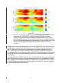
1
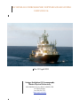
R.V. REVELLE HYDROGRAPHIC DOPPLER SONAR SYSTEM USER MANUAL Ver. 20 April 2011 Scripps Institution Of Oceanography Marine Physical Laboratory 8810 Shellback Ave, La Jolla CA 02093-0226 tel: 858-534-3863 fax: 858-534-7871 http://opg1.ucsd.edu 1 CONTACT NUMBERS: Rob Pinkel [email protected] 858-534-2056 Michael Goldin [email protected] 858-534-3863 Oliver Sun [email protected] 858-822-2580 Mai Bui [email protected] 858-534-4733 2 TABLE OF CONTENTS I. OVERVIEW: To the Chief Scientist:! 4 HDSS BACKGROUND! 4 HDSS OPERATIONAL CONCERNS! 7 II. INTRODUCTION:! 9 SYSTEM OVERVIEW! 11 ACCESSING DATA! 16 III. USER OPERATION: (For STS Personnel Only)! 19 STARTING/STOPPING THE HDSS! 19 SONAR DISPLAYS! 21 IV. TECHNICAL REFERENCE:! 22 HARDWARE! 22 DATA FLOW! 26 MATLAB PROCESSING! 28 TROUBLESHOOTING! 29 3 I. OVERVIEW: To the Chief Scientist: 0HDSS BACKGROUND The Hydrographic Doppler Sonar System (HDSS) on the R.V. Revelle provides profiles of absolute ocean current and acoustic scattering strength in support of scientific operations. The HDSS consists of a 50 kHz sonar which profiles to depths of 700–1100 m, and a 140 kHz system which profiles to 150–350 m. The system was created to provide measurements with higher depth-resolution than is available from commercial Doppler sonars. Both the acoustic pulse length and the angular width of an acoustic beam affect depth resolution. The HDSS sonars employ large transducers relative to the commercial systems in an effort to minimize acoustic beam-width. A comparison of velocity (Figure 1) and Shear (Figure 2) data from the HDSS sonars and the Revelleʼs 75 kHz ADCP is presented below.0 Just as ocean bathymetry is routinely collected from research vessels, the HDSS has the parallel tasks of monitoring ocean currents and acoustic scattering wherever the Revelle sails, while simultaneously supporting individual science missions,The established policy is to have the system running and recording data at all times that the ship is underway, unless restricted by political regulation or acoustic interference. Following extensive tests, it has been determined that operation of the HDSS does not interfere with simultaneous use of the Revelleʼs acoustic speed log, 3.5 kHz sub-bottom profiler, Simrad 12.5 kHz swath mapping system or RDI 150 kHz and 75 kHz ADCPs. Please do NOT turn off the transmitters on either HDSS sonar “just-to-be-sure”, without first contacting the Ocean Physics Group at Scripps. ## ADD DATA ACCESS FROM THE DISPLAY CONSOLE KEYBOARD ETC 4 0 Figure 1. A forty-hour record of Meridional velocity from the HDSS 140 kHz sonar(top), the 75 kHz ADCP (middle), and the HDSS 50 kHz sonar (bottom). The arrows in the lower panels indicate the field of view of the panel immediately above. The strong northward flows of the diurnal internal tide (red) fill the depth-range of the high-resolution (6m) 140 kHz sonar. The 50 kHz sonar can see the weaker currents below, with 22 m vertical resolution. Visiting science teams are welcome to use and keep HDSS data, at the discretion of the Chief Scientist of each Revelle leg. Operation of the HDSS is under the supervision of the SIO Shipboard Computer Group representative on board. Requests to initiate or cease sonar transmission and/or data recording should be addressed to this person. The computer tech can provide hard copies of the HDSS data while at sea or at the end of each leg, as well as guide the science team in the use and interpretation of the realtime displays. Following established UNOLS /NSF practice, the Chief Scientist can request proprietary use of the data for a period of two years following the cruise. If not requested, the data will be made publicly available immediately following the cruise. In either event,, copies of the HDSS data are archived by the Ocean Physics Group at SIO , who are available to assist with data processing concerns. 5 Figure 2. Meridional shear, the derivative of velocity with depth, from the data in Fig 1. The extremely fine gradients of velocity with depth are thought to be due to internal waves, fronts, and small-scale geostrophic features. A global census of these motions. 0The HDSS can be programmed to operate in a variety of modes. A nominal operation sequence is provided, in which both sonars transmit at 2 second intervals, phase-locked to the Revelle GPS. Single-ping (2-second) profiles are recorded. The depth resolution is 6 m for the 140kHz sonar and 22 m for the 50 kHz sonar. Modifications to this nominal format can be made, but only with prior discussion and approval from the SIO Ocean Physics Group. Please do not attempt to modify the operating sequence on your own! 0 6 HDSS OPERATIONAL CONCERNS To measure absolute ocean currents of order 0.06 m/s from a ship moving 6 m/s, the ships motion must be quantified to 1%. Higher precision is desireable. A host of instruments is interfaced to the HDSS to achieve this end. A calibration shift in any of these sensors can eliminate the possibility of real-time absolute current information. Often, errant sensors can be post-calibrated using the ships navigation and the HDSS as references. If real-time absolute velocity knowledge is necessary, it can be obtained simply by slowing down periodically and reducing the ratio of ship speed to ocean current speed. 0The precision of the HDSS0 is limited by the motion of surface gravity waves. These appear as a high-frequency noise on the subsurface signals of interest. They also perturb the boatʼs trajectory by ~1 m/s rms, in normal condition. If each wave crest represents an independent sample of the wavefield, (unlikely) the rms wave noise can be reduced to ~0.1 m/s by averaging over 100 wave periods, requiring 20 minutes or more. 0Efforts to remove the depth-averaged velocity are partially effective in removing waveinduced ship surging. Sonar range is degraded by the presence of bubbles under the ship. Bubbles are generated by breaking waves, hull slamming, and the ships bow thruster. If sonar performance is a priority, plan to transit slowly enough to avoid pounding. Avoid use of the bow thruster. 0 0The real-time HDSS display0 presents depth-time plots of velocity, shear, and scattering strength, in the format of Figures 1,2. The display allows the option of removing a reference velocity, calculated over some 0user specified “level of no motion”, from the velocity estimates at all depths. This greatly reduces the influence of navigational errors. It is often an insightful and practical display. The shear display 0presents the vertical derivative of velocity with depth. This is relatively free of navigational uncertainty and provides a fine-scale diagnostic of the motion fields being traversed. 0Displays of echo intensity document the concentration of zooplankton, the primary scattering targets for the HDSS. Increases of shipboard or oceanic noise are also seen in this display. The planktonic communities are layered vertically. Their horizontal variability is being mapped as the ship progresses. The maximum range attainable by the 50 kHz is strongly dependent on the presence of a “mid-water scattering community” that includes plankton, squid, and small fish. This community is seen as a second maximum in sonar intensity between 300-600 m depth. The diel vertical migration alternately provides enhanced scattering for the 140 kHz system at night and improved long-range performance of the 50 kHz system during daylight. The primary artifact present in HDSS data is a spurious apparent shear 0that in-fact stems from rapid variation of scattering 0strength with depth. This 0 occurs only when the ship is moving and 0is seen only in the direction that the ship is going. Beware of frontallike structures that migrate 0at dawn or sunset. Comparing velocity and intensity displays 7 provides insight. The magnitude of this artifact is proportional to ship speed. To quantify its presence, slow the ship or change course0 8 II.0 0INTRODUCTION: The R/V Revelle is equipped with a Hydrographic Doppler Sonar (HDSS) System which provides estimates of: • Absolute ocean velocity • Ocean shear • Acoustic scattering intensity • Scattering intensity gradient (plankton layering) The system consists of two 4-beam Doppler sonars and assorted support sensors (Figs. 1-2): • The “Deep Sonar” operates at 44 kHz and can profile to depths in excess of 1 km in favorable conditions. Its depth resolution is approximately 022 m. • The “High Resolution Sonar” operates in a band near 140 kHz, profiling with 06 meters resolution to depth of 150-350m, depending on weather bio-scattering conditions. Both sonars are configured in the conventional 4-beam Janus geometry. In plan, the beams are oriented 45° relative to the fore/aft axis of the shipʼs hull (Figure 1). The depression angle of each beam relative to horizontal is 60 degrees. The HDSS sonars transmit through a protective polyethelene “window” mounted flush with the shipsʼs hull. They are similar in principle to the commercial instruments found on many research vessels. The HDSS sonar beam patterns are significantly narrower than those of most commercial systems. The sonars transmit synchronously at 2-second intervals. Coded acoustic pulses are used. The sound scatters from plankton drifting in the water column. From the Doppler shift of the return echo, the relative speed between the ship and the water can be inferred. GPS, along with a variety of other support sensors, is used to infer the absolute ocean velocity. Precise calibration of the sonars and the various position sensors is critical to the extraction of ocean velocity. With the ship moving at 12 kts, a 1% error in the correction for ship speed corresponds to 0.06 m/s, a value comparable to typical currents in the thermocline. The HDSS produces three classes of data. Raw echo data are recorded in binary format and stored on revolving buffers on the HDSS analysis computers. Each sonar produces of order 1 TB / month and the most recent ~20 days are stored. Raw data are useful for diagnosing system behavior or developing new processing methods. They are NOT routinely transcribed or transferred off the ship. The first level of processing is done in real-time, producing single-ping profiles of echo intensity and a variety of echo covariance estimates, all averaged into fixed depth bins (corrected for the roll of the ship). These “Cov” data files are reduced in size by a factor of ~50 relative to the Raw data. Month-long records of Cov data are 20–30 G-byte. These files are available to the scientific party in near real time and are routinely archived. Calibrated scientific products 9 Figure 1. A plan view of the Hydrographic Sonar beam orientation, looking down from above. are generated in a second level of Matlab-based processing that is done at-sea in nearreal time by a networked computer. A variety of ocean-velocity estimates are produced, each using differing noise filtering criteria. The Matlab output is typically averaged over 10 1–5 minute intervals (user selectable). Each sonar produces 1–2 GB / month of minuteaveraged data. " The real-time estimates of absolute velocity are vulnerable to calibration shifts in the sonar and the various positional sensors. It is common to post-process the Cov files multiple times to adjust sensor calibrations. SYSTEM OVERVIEW The major components of the Hydrographic Doppler Sonar System (HDSS) include Fig.3: 1.The transducers, located in port & starboard wells recessed into the shipʼs hull. 2.The sonar electronics, mounted in NMEA boxes (one for each sonar). The 140 kHz is located in the Revelleʼs transducer compartment. The 50 kHz is located below the exercise room. 3.The HDSS interface unit (one for each sonar). 4.The Time Data Server (TDS) computer, located in the shipʼs computer laboratory. 5.The data acquistion and initial processing computers and displays (one for each sonar). 6.The advanced processing (Matlab) and display computer 7.Lab display screens (actually). 11 Figure 2. a) The port sonar well viewed from below, showing the 50kHz Deep Sonar (grey hexagonal array) and 140 kHz High Res. (rectangular) transducers. Figure 2. b) The starboard Sonar well, showing beam 2 forward (right) and beam 3 aft (left) for both 50kHz (grey hexagonal array) and 140kHz (rectangular) 12 Ship subnet 10.16.50.xxx Astech G12 GPS Time 1000 4.HDSS PCode GPS 6. HDSS Server USB Serial Astech ADU5 GPS Time PHINS VRU Pitch, Roll, HDSS Server HDSS Time Data System 5. Data Acquisition RAID 140kHz HDSS 140 kHz HDSS 50 kHz USB Serial USB Serial 100 BT 3. HDSS interface sonar 140kHz interface unit 2. Sonar Electronics 100 BT sonar 50kHz interface unit Taxi F/O ADAM A/D 50kHz NEMA box temperature RAID 50kHz 140kHz System: Controller, Receiver, Transmit Amps Taxi F/O 50kHz System: Controller, Receiver, Transmit Amps Tx Snoar Well temperature Snoar Well pressure Tx/Rx Accelerometer Rx 1. Transducers Fig 3. Revelle Hydrographic Doppler Sonar Data Acquisition System 13 14 Fig 4. USB 8 com serial box for TDS Fig 5. RAID for HDSS 15 ACCESSING DATA Data from the Hydrographic Sonar System exist in three stages. The first stage is "Raw" data, which is simply the digital output of the digital basebanding sonar receivers. This raw digital data is processed into "Cov" data files, which contain single-ping (every 2 s) covariance data which have been corrected for ship motions (pitch/roll/yaw) and averaged into range bins. Covariance data are formed in real time and recorded in parallel with raw sonar data on the local sonar machines (50 kHz and 140 kHz CPUs). Finally, an automated process on the HDSS Server accesses the covariance data on the sonar machines, copies the cov files across the network, and forms finished products in Matlab format, or "mat" files, which include quantities of scientific interest (water velocity, shear, scattering intensity) as well as environmental sensor data (GPS position, ship attitude) and engineering data (sonar transmit, receive, and processing parameters, electrical status). It is expected that the Mat-files will fulfill the immediate needs of most scientific users. Nevertheless, as improved post-processing algorithms become available, new Mat-file products can be formed by reprocessing the Cov files. Hence it is vital that covariance data are retained for future use. Raw Data Format " Binary file containing interleaved integer output directly from the sonar A/D converters. Also included in the file are a dasinfo header, containing HDSS-specific transmit, receive, and processing parameters, and TDS (time/position and environmental sensor) data corresponding to each ping sequence. " Covariance Data Format " Binary file containing single-ping, bin-averaged covariance and intensity data along with dasinfo and TDS data. Mat-file Data Format " Matlab 6 data file containing a 'sonar' structure of multiple-ping-averaged, motion-corrected covariance, dasinfo, and TDS data. Further Matlab routines (included by default) add data products in scientific units (velocites, shears, navigation). " 'sonar' has the basic structure: sonar = filename: dasinfo: cov0: int0: {42x1 cell} [1x1 struct] [170x1440x4 double] [170x1440x4 double] 16 cov: int: covs: covs0: TDS: datenum: sn: nbins: ranges: depths: beamvel: u: w: u_z: nav: U: U_z: yday: lat: lon: [170x1440x4 double] [170x1440x4 double] [170x1440x4 double] [170x1440x4 double] [1x1 struct] [1x1440 double] [170x1440 double] 170 [170x1 double] [170x1 double] [170x1440x4 double] [170x1440 double] [170x1440 double] [170x1440 double] [1x1440 double] [170x1440 double] [170x1440 double] [1x1440 double] [1x1440 double] [1x1440 double] Header data " filename " " The basenames of sonar raw and covariance files whose data are contained in this sonar struct are stored in this cell array " " " dasinfo " " HDSS-specific setup variables are stored here, organized in exact parallel to the binary C data structure. " " TDS " Time Domain Server, contains all recorded environmental sensor data, including GPS and VRU (vertical reference unit) Covariance data (cov, int, etc.) " Using the raw digital output of the sonar receivers, a lagged autocovariance of the received signal is computed. The result, which contains Doppler phase shift information, is averaged by range bin (time gate) and stored in cov. A zero-lag autocorrelation, which represents the sonar backscatter intensity, is stored in int. " The autocovariance procedure incorporates an matched filter which improves detection at the maximum ranges of the sonar. This filter attempts to search near an 'expected phase shift' caused by ship motions. The IIR time filter used to center the matched filter can cause filtering errors due to a bottom hit or sudden ship motions to 17 persist over a period of several pings. Therefore, the unfiltered covariances and intensities, indicated by a following '0', e.g., cov0, should be used when the ship is in shallow water or where ship's navigation data contain repeated spikes. " To allow for precise averaging across pings, a motion correction algorithm is also applied to the single ping covarince data. The correction estimator is produced from the ship's VRU (vertical reference unit) inertial measurements. This corrected data, stored in covs (and covs0), is the default version used in all subsequent velocity computations. Velocities exist in three successive reference frames: Beam coordinates: beamvel, ranges " Positive-inward Doppler velocity detected by each beam (1‚Äì4) are computed from binned, motion-corrected covariance data (covs) and stored in beamvel. The indices of sonar.beamvel are [bin x time x beam]. Ship coordinates: u, w, u_z, depths " Velocities from the four sonar beams are combined into horizontal velocity u (Re + Im parts) and vertical velocity w in the ship's frame of reference. The ship frame is a right-handed coordinate system: Re u is pointed forward (toward the bow), Im u is across (toward the port side), and w is positive up. Vertical shear (du/dz) is placed in the field u_z. Indices are [bin x time]. Earth coordinates: U, w, U_z, depths " Using the heading and navigation information from the ship's GPS units and Vertical Reference Unit (VRU), the horizonal ship frame velocities u are transformed to earth frame velocities U (Re = East, Im = North) and vertical shear of horizontal velocity (U_z). Indices are [bin x time]. " Several useful fields are also included at the root level of sonar (datenum, yday, lat, lon) datenum " the TDS timestamp, in matlab datenum format. In multiple-ping-averaged sonar data, timestamps represent the time of the first ping included in the average. " yday " The decimal yearday, which includes a integer day (Jan 1 = yday 1) and a decimal part of days since midnight. " lat/lon/nav " Navigation data as recorded by the ship's GPS. nav is the ship's velocity (u + iv) in Earth coordinates. 18 III. USER 0 OPERATION: (For STS Personnel Only) 0STARTING/STOPPING THE HDSS 1.Turn on the four Macintosh Mini Computers 2.Turn on Sonar Power Supplies and “OPG Doppler Sonar Interface Units” 3.Start The SonarTDS command line program. a.Check the setup TDS file: double click on the file “TDS_Setup” on the TDS computerʼs destop. Its format should be the same as the example in Appendix III. b.Double click on the “Start TDS” icon on the TDS computerʼs desktop. c.The ”Terminal” application will start and run the “SonarTDS” executable in a terminal shell 4.The TDS will initialize serial ports for each sensor data stream from the 0 and begin to run. Verify that all sensors are reporting reasonable values and no “Missing string xxx error” message is displayed on the TDS screen. 5.With the TDS running, either sonar can be started up. To do so: 6.Start The SonarAcq command line program and SonarDAS monitor application. a.Check the setup Sonar file: open the text file “default.hdss_setup” in the HDSS folder using the TextEdit app. Its format should be the same as the examples in Appendices I, II. Change the run name parameter to reflect the current leg name. (i.e.sonarRec.runname = ʻ50kHz_KNOXnnRRʼ;) b.Make sure that the Ammeter on the power supply is not fluctuating (indicating that the system is still pinging). If it is still cycling, manually stop the unit before continuing (see section “Manually Stopping Sonar Controller, below) Note: when pinging, the 140kHz unit will show very small fluctuations, only a few tenths of an amp. The 50 kHz system has pronounced Ammeter fluctuations when transmitting. c. Press the reset button and wait for the ready indicator to light. DO NOT PRESS THE RESET BUTTON IF THE SONAR CONTROLLER IS CYCLING! If necessary manually stop the controller first. d.Double click on the “Start Sonar” icon on the 140 kHz and 50 kHz computerʼs desktop. This activates an applescript that: starts the “SonarACQ” command line program and the “Sonar DAS” application. e.Select the data directory for “Sonar DAS”. f. The ”Terminal” application will start and run the “SonarACQ” executable in a terminal shell. g.The SonarAcq will initialize the system and begin to run. Verify that the sonar and all sensors are reporting reasonable values. Data are written to primary and secondary disk files with paths specified in the setup file (default.hdss_setup). These paths typically point to 2 external firewire drives mounted in the rear of the 50kHz rack. The filenames are auto-generated from the setup file with a date code appended. (see example below) 7.Set SonarDas monitor app to the current data directory. a.click the “Choose Directory” button and navigate to the current RAW data directory i.e. HDSS_50k_Data_Copy1/50kHz_KNOX18RR_RAW. The application will start 19 plotting the latest sonar data from that directory in the “Sonar Playback Window”. The recorded TDS data are displayed in the “TDS Graph Window”. b.DO NOT PRESS THE “Run TDS” OR “Run Sonar” BUTTON ON THE SONAR DAS WINDOW! These controls are deprecated and have been removed in the latest release. 8.To stop either sonar type <q> and press <enter> key from their respective Terminal shells. To re-start the sonar press the <key up> from the Terminal to select the last command, <path>SonarAcq, and press <enter> key to restart. If the sonar fails to quit and is still pinging manually stop the sonar controller as instructed below. If the HDSS does not start 1.Verify 0 that TDS program is running. If not, stop the SonarTDS and SonarAcq programs. type <q> and press <enter> key from their respective shells 2.If TDS is working, stop the SonarAcq program by typing a <q><ret>, reset the “OPG Doppler Sonar Interface Unit” and restart the SonarAcq program. Manually stopping the Sonar Controller 1.Double Click the application “GoSerial” or “CoolTerm” from the applications directory. It should currently be set to the Sonar Controller serial port (usbserial-A700f4f7) and baudrate (19200) 2.After typing a few returns you should get a colon prompt: 3.Type an <h> to halt the sonar controller. The controller should now be stopped. 4.Make sure the ammeter on the supply front panel is now stable indicating that sonar transmission has ceased. 20 SONAR DISPLAYS 0 " Data Plotting Options: The SonarAcq program runs in terminal mode. It only outputs diagnostic text with a small portion of the raw data each ping just before the transmit pulse is generated and the first and the last TDS packet spanning that ping. The SonarDAS application can be run to plot a real time intensity of the ping as well as TDS data. The program is automatically started after double clicking the “Start Sonar” icon. " " It reads the data files specified by the “Choose Directory” button on the main window. Selecting the directory of the current acquisition path, (i.e., HDSS_50k_Data_Copy1/ 50kHz_KNOX14RR), should automatically plot the latest data acquired. De-selecting the “Realtime Mode” checkbox and using the sliders allows reviewing historical data. 0 21 IV.0 TECHNICAL REFERENCE:0 A. HARDWARE refer to figure 3 1.The transducers, along with accelerometers, thermometers and pressure sensors, are located in two 12ʼx5ʼx4ʼ wells in the shipʼs hull, located just aft of frame 57, on the port and starboard sides of the ship. Starboard facing beams are mounted in the starboard well, etc. Separate transmit and receive transducers are used for each Deep Sonar beam. Each transducer is a mosaic of hexagonal sub-elements. Single transducers are used for both transmit and receive in the 140 kHz system." • In an effort to maximize reliability, there are no active electronic elements in the underwater acoustic components residing in the transducer wells. 2.Cables from all well-mounted transducers and sensors are routed through stuffing tubes in the forward ends of the wells, into the Revelle transducer void compartment between frames 55 and 52. " 3.The 140 kHz Sonar cables lead directly to a bulkhead mounted NMEA box that contains sonar electronics (Fig. 6). The Deep Sonar cables are lead upward one deck to a similar NMEA box mounted just below the Revelleʼs exercise room (Fig. 7). 22 Revelleʼs sonar void compartment Figure 6. 140 kHz: The NMEA box in the housing the 140 kHz Hi Res sonar electronics. Figure 7. 50 kHz: The NMEA box in the compartment below the Revelleʼs exercise room 23 4.Within each NMEA box are found sonar power supplies, transmit power amplifiers, TR switches (140 kHz only) and tuning boxes, receive pre-amplifiers, digitizers and an electro-optical converter. A “sonar controller” that generates the frequencies required for transmit and orchestrates system timing is also located in each box. Signals from the center and the outer ring of the 50 kHz receivers are recorded separately. Thus there are eight receive channels in the 50 kHz NMEA box, vs. four for the 140 kHz system. " 5.Signals from the accelerometer, temperature, and pressure sensors in the transducer wells, are digitized by an ADAM A/D Module, housed in the 140 kHz sonar NMEA box. 6.The HDSS interface connects to the sonar electronics NEMA Boxes via a high speed point to point fiber optic data link using the TAXI protocol. Data from the NEMA box is demultiplexed into a down-converted doppler data stream and two auxiliary data RS232 serial streams. The doppler data stream is formatted into ethernet TCPIP packets and sent to the data acquisition computers (Fig.8). The serial data streams are split into individual RS323 jacks in the back. The first connects the sonar controller (located in the NEMA box) to the the acquisition computerʼs serial to USB port. The second connects the ADAM A/D serial data output containing the accelerometer, sonar well temperature, and sonar well pressure to one of the TDS computerʼs serial to USB ports. 7.The HDSS is operated from a Console located in the Revelleʼs computer laboratory (Fig. 8) by personnel from SIO Shipboard Computer Group. From here, AC and DC power, and digital control instructions are provided to the sonars below through two Doppler Sonar Interface Units. Digitized data are received from the sonars, merged with data from supporting sensors and processed to provide real time estimates of velocity and scattering intensity. " 8.The HDSS Control Console consists of an independent power supplies for each sonar, along with two Macintosh mini computers for data recording and preliminary processing (Fig. 9). The system is synchronized by a third computer, (screen on upper right), which runs the Time Data Server (TDS) program. The “Time Data Server” orchestrates environmental data streams from the ships GPS, the Ashteck ADU2 positional sensor, a stand-alone GPS G-12 timing signal, the gyro compass, the PHINNS ships orientation system, sonar well temperature, pressure, and acceleration, among others. All operations are linked to a GPS time-base (provided by an Ashtech G12 receiver located on the shipʼs bridge.). Timing and all ancillary data are decoded and provided to the sonar operations programs by TDS. The TDS program does not itself record this data. . 9.Data Processing: The lower left computer in the HDSS Console receives and processes data from the 140 kHz sonar while the lower right computer handles the 50 kHz Deep Sonar. Each runs a program called “R/V Revelle Sonar” that receives digital sonar data from the NMEA electronics boxes and environmental data from the TDS. The sonars are synchronized such that the short transmit from the 140kHz system occurs coincident with the final milliseconds of the Deep Sonar transmission. In this way, near-range contamination of the 140 kHz signal is minimized. Single-ping (2second) averages of echo Covariance data are written on hard drives in the rack behind the analysis computers, along with the most recent Raw data, stored in revolving buffers. 24 10.The fourth HDSS computer, also located in the console, has access to the data drives. It reads the most recent Covariance data and forms time-averages (typically 1 min or 5 min) of ocean velocity, acoustic intensity, and other quantities of scientific interest, using Matlab scripts. Data are displayed on the upper right screen in the HDSS Console 11.Raw data display screens. Two flat screen displays in the Shipboard Computer Group display console in the Computer Lab present real-time raw data from the HDSS sonars. And These displays are primarily a diagnostic of the instantaneous operating state of the system. 25 B. DATA FLOW HDSS Data Acquistion Machines (50 kHz/140 kHz) Raw, interleaved output from the sonar A/D converters are stored as RAW binary files on the external RAIDs which are connected to each acquisition machine and secured in the machine rack. Bin-averaged covariance data, stored as COV binary files, are written to disk in parallel with the corresponding RAW files. A nominal size limit (originally set as a convenient size which avoids filesystem limits) is set for each file type. The RAW and COV data files are maintained as a FIFO configuration: the oldest files are automatically removed by a cron job once disk usage exceeds a preset limit. Typically, about 21 days of RAW data are kept on disk, but the COV data (which have a much higher removal threshold) are only removed if the disk becomes dangerously full. HDSS Server The HDSS Server provides four main services: 1) backup of covariance data, 2) postprocessing of covariance into scientific quantities (e.g., ocean velocity, shear, and backscatter intensity), 3) near-realtime displays of scientific data, accessible over the ship's network on on a series of HDSS Server web pages, and 4) user access to data, both as covariance files and as post-processed data in Matlab format. Automated tasks behind these services are performed by a sequence of UNIX shell and Matlab scripts. These are initiated at regular intervals (< 10 mins) by an entry in the root (user?) crontab. A lockfile is created at the beginning of the cron job to prevent multiple executions of the (possibly long) Matlab processing stage. If execution completes normally, the lockfile is removed prior to exit. A local mirror of single-ping covariance data for each sonar (50 kHz and 140 kHz) is maintained using rsync, over ssh connections to each sonar acquisition machine. The mirror is physically located on an external FireWire 800 drive, labeled Server_EXT_xx, which is secured in the back of the server rack. All covariance files copied by rsync remain on the server even if they are removed from the acquisition machines by the FIFO mechanism. Averaged covariance data are stored in Matlab files, also on the external drive, with one file per day. At midnight each day, a new file is created containing a new 'sonaravg' structure with a full timegrid (datenum field) but with all other data initialized to NaN. As new covariance files become available through rsync, the data fields in sonaravg are updated. During each update, velocity and shear are computed from averaged covariances and added to the sonaravg structure. 26 The update process has a maximum lookback setting in days, typically set at 3–5. Missing daily Matfiles within this limit are formed if covariance data are available. Once sonaravg is brought up-to-date, a set of Matlab routines create plots of beam velocities, backscatter intensity per beam, and zonal and meridional absolute velocity and vertical shear. All plots are available on the HDSS Server website and are set to auto-refresh once the page is loaded. The default plot is a combination velocity-shear plot in which the color scale indicates velocities and simple shading indicates vertical shears. Plotting limits and scales, as well as the time window covered by the plots, are user-configurable. The number of pings per average is also user-configurable in Matlab, and is typically set to 2 or 4 minutes. Longer averages are recommended during noisy sea states or low backscatter conditions; however, shorter averages are preferred if further processing, e.g. explicit noise rejection or navigation correction, is anticipated. The current version of the plotting routines does not handle different averaging intervals within the plotting window; if the ping averaging is changed, old Matfiles created using the previous averaging interval should be removed from the Matfile directory. New Matfiles will be backfilled (to the lookback limit) by the updater. The hdssMatlab scripts from the HDSS Server are available for download and may be used with minor modification (i.e., to point to local data) or as templates for local data processing. The most useful Matlab scripts are described in the following section00 27 C. MATLAB PROCESSING Creating Matlab files of velocity and shear from covariance data To create a single Matlab file from a collection of covariance data: Place the covariance files in a separate directory and assign the following variables in your Matlab workspace: >> sourceDir = [your directory path] >> Navg = [pings to average, 30 pings * 2 s/ping = 60 s averages] Run the following (with the hdssMatlab directory in your path): >> sonaravg = AverageCovFiles(sourceDir, Navg) This will return a sonaravg structure containing bin-averaged, motion-corrected covariances and backscattering intensities, along with header and TDS data. To convert covariances to scientific units of velocity and shear, do >> sonaravg = ProcessCov(sonaravg, csound) " where csound is optional and specifies a local sound speed velocity. (ProcessCov may be re-run on the same sonaravg at any time using a different csound if desired).0 28 D. TROUBLESHOOTING If System fails to start or hangs during operation: ! Check Power Supplies: " The green lamp on the top of the NEMA box should be lit indicating power from rack supply is present. You can also check the supply outputs inside the NEMA box. The wires going into the fuse panel are color coded: " Yellow = +5 V " Blue = -5V " Green = common " Red = +20V " Brown =-20V " Grey = common " There are spare supplies and fuses located in the 0spares box in the forward electronics store room if you need to replace them. 0 Power supplies are good but sonar controller fails to load after SonarACQ started: 1.Quit sonar application and start the Zterm application. 2.Set baud rate to 19200 by clicking baud button on lower left of control window. 3.Set channel to KeySerial1. 0 (this corresponds to the #1 port of the Keyspan USB dongle) 4.Type a few returns. Each should be accompanied by ʻ:ʼ prompt. 5.If you get a prompt type lower case L. This should give you a list of setup parameters. 6.If you receive no prompt the controller, the USB/serial dongle, or serial cabling is malfunctioning. Repeat serial and USB connectors. Restart and repeat the test. Time Data Server (TDS) : • To stop the TDS type <q> and press <enter> key in the TDS Terminal. (if the computer freezes press and hold the power button on the rear-right side of the mac mini) • Re-start the Computer. • Start the TDS program by double click the “Start TDS” icon on the desktop. Acquisition should start and a terminal output should indicate sensors being acquired • Start the Sonar program by double clicking the “Start Sonar” icon on the desktop • From the “SonarDAS” application select the “Choose Directory” button on the lower left “Sonar Playback” window. Navigate to the current data directory and click the “Open” button. The screen should now be updating (realtime mode is selected by default” 29 Checks before starting 50kHz and 140kHz Revelle Sonar applications: 1.Check that all the cables are firmly connected. 2.Check configuration: • Open “default.hdss_setup” 3.Start the sonar by pressing the “Start Sonar” button 30