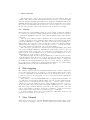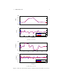
1
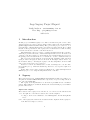
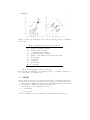
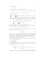
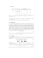
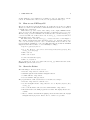
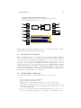
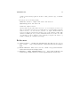
Linköping University Electronic Press Report Lego Segway Project Report Patrik Axelsson and Ylva Jung Series: LiTH-ISY-R, ISSN 1400-3902, No. 3006 ISRN: LiTH-ISY-R-3006 Available at: Linköping University Electronic Press http://urn.kb.se/resolve?urn=urn:nbn:se:liu:diva-89973 Technical report from Automatic Control at Linköpings universitet Lego Segway Project Report Patrik Axelsson, Ylva Jung Division of Automatic Control E-mail: [email protected], [email protected] 16th March 2011 Report no.: LiTH-ISY-R-3006 Address: Department of Electrical Engineering Linköpings universitet SE-581 83 Linköping, Sweden WWW: http://www.control.isy.liu.se AUTOMATIC CONTROL REGLERTEKNIK LINKÖPINGS UNIVERSITET Technical reports from the Automatic Control group in Linköping are available from http://www.control.isy.liu.se/publications. Abstract This project was a part of the course Applied Control and Sensor Fusion (http://www.control.isy.liu.se/student/graduate/AppliedControl/ index.html) during summer and fall 2010. The goal of the course was to be a practical study of implementation issues, not always encountered in the life of a PhD student. A segway was constructed using a LEGO Mindstorms NXT kit and a gyro, and the goal was to construct a self balancing segway. To do this the motor angles and the gyro measurements were available, and a working Simulink program. The main focus in this project has been to construct an observer. The segway can be used for demos in basic control courses, and a manual can be found at the end of the report. Keywords: segway, manual, observer, lego mindstorms Lego Segway Project Report Patrik Axelsson – [email protected] Ylva Jung – [email protected] 2011-03-16 1 Introduction In this project a LEGO segway robot has been built as a part of the course Applied Control and Sensor Fusion (http://www.control.isy.liu.se/student/ graduate/AppliedControl/index.html). The goal of this project course is to be a practical study of implementation issues, not always encountered in the life of a PhD student. A short presentation of the segway can be found in Section 2. The modeling is described in Section 3 and the controller in Section 4. The initial plan for the project was to construct and implement an H∞ -controller, and if the project time allowed it, construct and implement an observer. We started out on an H∞ -controller, but since we did not like the way of implementing an observer by integrating a sensor measurement we soon switched to observer construction instead. The observer is presented in Section 5 and works well on simulated data, but when trying it on the real segway it did not work at all. To investigate why we tried to log the measured data by connecting the segway to the PC, using Bluetooth and a USB cable, but we did not succeed, see Section 6. In Section 7 a short user manual can be found, describing how to use the existing programs (for e.g. small demonstrations), and how to develop and compile new programs. If there had been more time, we had most likely tried to design and implement an EKF and/or proceed to design and implement an H∞ controller. 2 Segway The segway used is based on LEGO Mindstorms NXT and assembled according to [1]. All parts are standard LEGO Mindstorms components, except for a single direction gyro sensor from HiTechnic. The segway is an implementation of an inverted pendulum and is a nonlinear system. The nonlinear model and the linearised model used in this project are further presented in Section 3. Inputs and outputs The actuators of the segway are two DC motors, one connected to the left wheel and one to the right. To control these actuators, the controlled input is: • voltage to the motors recalculated to two PWM signals to the left and right DC motor. Some of the segway state variables are measured and the outputs from the segway are: • the DC motor angles θml and θmr 1 3 MODEL 2 Figure 1: Side view and plane view of the two-wheeled inverted pendulum modeled [1]. Table 1: Physical parameters used in the model. g gravitational acceleration Jm DC motor moment of inertia Jw wheel moment of inertia Jφ body yaw moment of inertia Jψ body pitch moment of inertia L distance of the mass center from the wheel axis m wheel weight M body weight n gear ratio R wheel radius W body width • the body pitch angular velocity, ψ̇ from the gyro. The other states, including the body pitch angle ψ, have to be calculated, and therefore an observer will be used in this project. 3 Model The model used is derived by [1]. Since the segway has been built in the same way as the segway the models were developed for, these are judged to be valid in this project. Figure 1 shows a simplified two-wheeled inverted pendulum from the side and from the top, with the coordinates used in the report. These are θ: average angle of left and right wheel, θl and θr ψ: body pitch angle φ: body yaw angle and some parameters are presented in Table 1 (for the numerical values, see [1]). 4 CONTROLLER 3 Lagrange equation leads to a description of the motion, (2m + M )R2 + 2Jw + 2n2 Jm θ̈ + M LRcosψ − 2n2 Jm ψ̈ − M LRψ̇ 2 sinψ = Fθ (1) 2 2 2 M LRcosψ − 2n Jm θ̈ + M L + Jψ + 2n Jm ψ̈ − M gLsinψ− M L2 φ̇2 sinψcosψ = Fψ (2) 2 W 1 mW 2 + Jφ + Jw + n2 Jm + M L2 sin2 ψ φ̈ + 2M L2 ψ̇ φ̇sinψcosψ = Fφ 2 2R2 (3) These equations are nonlinear but can be linearised around a point of equilibrium, in this case the upstanding position of the segway (ψ → 0 ⇒ sinψ → ψ, cosψ → 1 and higher order terms are neglected). Equations (1)-(3) can then be approximated as (2m + M )R2 + 2Jw + 2n2 Jm θ̈ + M LR − 2n2 Jm ψ̈ = Fθ 2 2 2 (4) M LR − 2n Jm θ̈ + M L + Jψ + 2n Jm ψ̈ − M gLψ = Fψ 2 1 W mW 2 + Jφ + Jw + n2 Jm 2 2R2 (5) φ̈ = Fφ , (6) where Fθ,ψ,φ are the forces in the θ, ψ, φ directions, respectively. The connection between θ and ψ and their derivatives is described in Equations (4) and (5), and φ in Equation (6). So with the state vectors x1 = θ ψ θ̇ ψ̇ T , x2 = φ φ̇ T (7) and the expressions for Fθ,ψ,φ as in [1], the motion equations can be rewritten and divided into two separate state space models, x˙1 = A1 x1 + B1 u (8) x˙2 = A2 x2 + B2 u (9) T where u = vl vr are the left and right motor voltages. In the model in Equation (8), with the equations handling the upright position (no turning possibility needed), vl = vr , so therefore these are simplified to the one input signal, u, the voltage to the motors. The angles θ and ψ are in radians and the angular velocities θ̇ and ψ̇ are in radians/s. Since this project has focused on the control of θ and ψ, only the model described in (8) has been considered. The nonlinear state equations are linearised around the upstanding position and are thus only valid around that point. 4 Controller The controller implemented in [1] is a modified linear quadratic controller, with a feedback gain and an integral gain (to help control the position of the segway). The weight matrices are Qlqr 1 0 = 0 0 0 0 6 · 105 0 0 0 R 0 0 1 0 0 0 0 0 1 0 0 0 0 , 0 4 · 102 T Rlqr = 1 · 103 0 0 1 · 103 (10) with xlqr = θ ψ θ̇ ψ̇ (θ − θref ) . So the Qlqr (2, 2)-element is the weight for ψ and the Qlqr (5, 5)-element is working on an added state, the integrated difference 5 OBSERVER 4 Figure 2: An overview of the modified LQ controller [1]. Cθ denotes the conversion from x1 to θ. between the angle θ and the reference θref , see Figure 2 for the Simulink block diagram of the controller. The controller has not been evaluated or improved in this project. 5 Observer The observer that was implemented in [1] integrated the measured angular velocity from the gyro. One thing that you learn in a basic course in signal processing is that the measured signal from many sensors are noisy and influenced with drift. That is, a constant sensor error will grow without limits, when integrating the signal. Integrating this signal directly will therefore be a bad decision. Instead we developed a model based observer to cope with this problem. The segway is a nonlinear system, that means, a nonlinear observer should be used, e.g. Extended Kalman Filter (EKF). Since we used a linearised model of the segway in upstanding position, as described in Section 3, a stationary Kalman Filter (KF) was used. The system can be described by a continuous state space model according to (8), ẋ1 = Ax1 + Bu, (11) T where x1 = θ ψ θ̇ ψ̇ , A and B are system matrices and u is the voltage to the motors, see Section 3 and [1] for more details. 5.1 Design We augmented this model with one more state δ in order to take the drift of the gyro into consideration. The new model, where we also have included a noise model, can be written A 0 B B 0 ẋ = x+ u+ w, (12) 0 0 0 0 1 | {z } Ā | {z } | {z } B̄ Ḡ T T where x = θ ψ θ̇ ψ̇ δ is the augmented state vector and w = w1 w2 is the noise vector. The measured signals are the angular velocity of the body from the gyro and the motor position of the two motors. First, we model the measured angular velocity as y1 = ψ̇ + δ = 0 0 0 1 1 x. (13) It is a bit more tricky to find a relationship between the measured motor angles and 5 OBSERVER 5 the states. A glance at the existing solution gave us θ= 1 1 (θl + θr ) = (θm,l + ψ + θm,r + ψ) = 2 2 1 = (θm,l + θm,r ) + ψ = θm + ψ, 2 (14) where θl and θr are the angles of the left and right wheel, θm,l and θm,r are the angles ∆ 1 2 of the left and right motor, which are measured, and θm = measurement equation can be written (θm,l + θm,r ). The second (15) −1 y2 = θm = 1 0 0 0 x, and the complete measurement equation with measurement noise added is at last obtained as 0 0 0 1 1 y= x + e = C̄x + e. (16) 1 −1 0 0 0 Simple calculations show that the model is observable, i.e., the observability matrix O has full rank. The stationary KF can be written as x̂˙ = (Ā − K C̄)x̂ + B̄ K u y , ĀP + P ĀT − P C̄ T R−1 C̄P + ḠQḠT = 0, T K = P C̄ R T −1 , (17a) (17b) (17c) T where R = E ee and Q = E ww . We have also assumed that the cross correlation between the process noise w and the measurement noise e is zero. The Matlab function lqe has been used to calculate the observer gain K. The covariance matrices for the process noise and measurement noise are chosen as Q= R= 5.2 20 0 0 0.1 (18a) 0.01 0 0 . 0.001 (18b) Implementation The observer has to be discretised before it can be implemented in the Simulink diagram. The discretisation is made with zero order hold, that is xk+1 = Ad xk + Bd uk , (19a) yk = Cd x, (19b) Ad = eĀTs , (20a) where Z Bd = Ts eĀt B̄dt, (20b) 0 Cd = C̄. The sample time Ts is 4 ms. (20c) 6 DATA LOGGING 6 The measured gyro data are in degrees/s but they are given with an offset. An estimate of the offset is obtained if the measured data is averaged over several readings while the segway is standing still. This is done during the initialisation task in the Simulink diagram. The offset is then subtracted from the measurement before it enters the observer. A transformation from degrees/s to rad/s also has to be done both for the gyro data (after the offset is removed) and for the measured motor angles. 5.3 Result The linearised model was simulated with our observer. Figure 3 shows the estimated θ, ψ, θ̇ and ψ̇. Note that the estimation starts after 1 s because the first second is used to perform the initialisation task. We can see that the estimated states follow the true states well. There are some differences in the beginning of the second state but it is less than 5◦ which we thought would be sufficient. These differencies probably stem from the peak in the fifth state, δ, causing a discrepancy between the true and estimated ψ̇, thus leading to an error in the ψ state. We have also compared our estimates with the estimates from the existing observer in [1] and they are more or less the same. The state δ, that describes the drift in the gyro, is shown in Figure 4. The controller is obviously able to hold the segway in an upstanding position with our observer during the simulation. But when we download the observer to the real segway and run it, the segway can not be controlled to an upstanding position. We therefore tried to save the estimates from our observer and the existing one to see how different they are on the segway, see Section 6. The different behaviour of the segway in simulation vs. reality is probably because of the linearisation made in Section 3; the model and controller are linear but the reality is nonlinear. One way to better imitate this situation would be to implement the nonlinear system in the simulation model, to be able to tune the Q, R matrices in eq. (18) in a more suitable way. Another solution would be to use a time varying Kalman filter instead of the time invariant KF we have used. 6 Data logging The obtained observer works very well during simulations, but not when compiled and used on the segway. Therefore we wanted to log the measured data from the segway to better see what happens and why this did not work. Our intention was to see how to tune the observer to the real segway, i.e., choose new Q and R matrices that fit the true system better. It is possible to connect the LEGO NXT brick to a computer using either Bluetooth or a USB cable, and we started using the Bluetooth connection since this means the segway can move around freely, like it is supposed to. But we could not get the connection to work, the COM port did not register anything being sent or recieved. To use the USB connection an additional program, USBlib, had to be downloaded that did not agree with the firmware version used. We changed back to an older version of the firmware, but this took away the possibility to compile and download new programs to the segway, and we decided not to proceed with this. So sadly enough we did not succeed in logging data, which makes it hard to tell what the problem with our observer was. 7 User Manual This section describes how to build the Simulink diagram and download the program to the segway. A description of how to use the segway is also included. There is also 7 USER MANUAL 7 3000 θ [deg] 2000 1000 0 −1000 0 5 10 15 20 25 30 10 ψ [deg] 5 0 True Estimated −5 −10 0 5 10 15 20 25 30 20 25 30 Time [s] (a) State one and two. θ dot [deg/s] 500 0 −500 0 5 10 15 40 ψ dot [deg/s] 20 0 −20 True Estimated −40 −60 0 5 10 15 20 25 30 Time [s] (b) State three and four. Figure 3: The true states (blue) and the estimated states (red) with our observer. 7 USER MANUAL 8 1 0 −1 δ [deg/s] −2 −3 −4 −5 −6 −7 0 5 10 15 20 25 Time [s] Figure 4: The estimated offset of the gyro, i.e., state five. 30 7 USER MANUAL 9 another Matlab toolbox available at [3] which is good if you only want to test the sensors. No instructions for the second toolbox are presented in this report. 7.1 How to use NXTway-GS The given controller in [1] uses the Matlab toolbox Embedded Coder Robot for LEGO Mindstorms NXT or for short ECRobot NXT. Information about the toolbox and how to install can be found in [2]. All the files for [1] can be found on the desktop of the computer RTLT-12 in the directory Segway filer. The Matlab files can then be found under nxtway_gs\models. The file nxtway_gs.mdl is a simulation model that uses the controller in nxtway_gs_ controller.mdl. The rest of this section focus on nxtway_gs_controller.mdl since it is this file that is used on the segway. The main window of the file nxtway_gs_controller.mdl can be seen in Figure 5. The controller is implemented in the subsystem nxtway_app. Press the button Generate code and build the generated code to do what it says. However, there is some problem with the installation so the only thing that happens is that the Simulink diagram is built. The rest has to be done manually according to • Open C:\cygwin\bin\bash.exe • Go to the directory c:\Document and Settings\rtadm\Desktop\Segway filer\ nxtway_gs\models\nxtprj • Write make all • Write make rxeflash • Connect and start the segway • Write sh ./rxeflash.sh The program is now on the robot and is called nxtway_app which is the same as the Simulink subsystem described above. 7.2 Start the Robot The main things to know about the robot is: 1. Press the orange button to start the robot. 2. Walk through the menus with the triangular buttons. 3. Confirm with the orange button. 4. Go back with the dark gray button. The program that is downloaded in Section 7.1 is started according to: 1. Press the orange button to start the robot. 2. Use the triangular and the orange buttons to choose My Files/Software files/ nxtway_app. 3. Choose the alternative called run and confirm with the orange button. 4. The main menu for the NXT program is now visible. The display shows how to continue. 5. The robot must be held still in an upright position when the start button (right triangular button) is pressed. Release the robot when a beep sounds. 7 USER MANUAL 10 NXTway-GS Controller Model based on Rate Monotonic Scheduling This model consists of four parts : Device Inputs, Device Outputs, Task Scheduler, and Application Task Subsystem. Disclaimer: LEGO(R) is a trademark of the LEGO Group of companies which does not sponsor, authorize or endorse this demo. LEGO(R) and Mindstorms(R) are registered trademarks of The LEGO Group. 3 int32 In1 C C theta_m_l Revolution Sensor Interface Port = C Priority = -1 4 int32 In1 B theta_m_r Revolution Sensor Interface1 Port = B Priority = -1 6 int32 task_init ### OSEK Tasks ### task_init: Init task_ts1: 0.004 [sec] task_ts2: 0.02 [sec] task_ts3: 0.1 [sec] ExpFcnCalls Scheduler Priority = 0 task_ts1 task_ts2 task_ts3 int8 task_init_fc task_ts1_fc task_ts2_fc 1 pwm_l Servo Motor Interface1 Port = C Priority = 1 int8 B 2 pwm_r task_ts3_fc nxtway_app S2 Servo Motor Interface Port = B Priority = 1 uint8 BTTx sonar Ultrasonic Sensor Interface Port = S2 Priority = -1 5 uint16 Bluetooth Tx Interface Priority = 1 uint32 Freq uint32 Dur S4 gyro Gyro Sensor Interface Port = S4 Priority = -1 2 uint8 BTRx Sound Tone Interface Priority = 1 ## Requires only MATLAB products ## Generate code from task subsystem using RTW-EC bluetooth_rx 1 Bluetooth Rx Interface Priority = -1 ## Requires additional 3rd party tools ## Battery Voltage Interface Priority = -1 Download (NXT enhanced firmware) Generate code and build the generated code uint16 battery Download (SRAM) Click the annotations to generate/build code and download it into NXT System Clock Interface Priority = -1 Figure 5: The main window of the file nxtway_gs_controller.mdl. The controller is implemented in the subsystem nxtway_app. 7.3 Develop new Programs This section describes how you can develop your own program in ECRobot NXT. It is best to start with nxtway_gs_controller.mdl since all the necessary settings are correct in that file. Save the file as something new, e.g. my_terminator, and you are ready to develop. Start by renaming the subsystem nxtway_app to a name of your choice, e.g. terminator. Then, right click on the button Generate code and build the generated code, choose Annotation Properties... Finally, change the name of the system you want to build in the ClickFcn text editor. In other words, change from nxtbuild(’nxtway_app’,’build’) to nxtbuild(’terminator’,’build’). You are now free to implement your on program. The program should be implemented in the subsystem you just renamed, i.e., terminator. 7.4 Possible Error Messages. You can find the solutions of some errors that may occur in this section. • If Error executing callback ’ClickFcn’ Error using ==> nxtbuild at 149 ### Failed to create nxtprj directory for model: nxtway_app arises when you press the button Generate code and build the generated code, then it is probably because you are in the nxtprj folder with Cygwin. Go back one folder and try again. • If you do not get the message filename.rxe=xxxxx when you type sh ./rxeflash.sh in Cygwin, there might not be enough space on the NXT. Delete pro- REFERENCES 11 grams not used and try again. It can also be that you have forgot to turn the robot on. • If you get an error message saying ### Model failed to compile with strict bus check on ### Turning strict bus check off ... Model has compile errors. when you have pressed the button Generate code and build the generated code, then open the file rtwbuild. Set a breakpoint at row 201 and then press the button Generate code and build the generated code again. Matlab will now stop at row 201 in rtwbuild and you have access to the variable newExc. The variable is a MException object and contains information about the error. The error message you are looking for can be found if you dig into the causes, e.g. newExc.causes{1,1}.causes{1.1}.message. References [1] Yorihisa Yamamoto. NXTway-GS (Self-Balancing Two-Wheeled Robot) Controller Design. http://www.mathworks.com/matlabcentral/fileexchange/ 19147 [2] Takashi Chikamasa. Embedded Coder Robot NXT. http://www.mathworks. com/matlabcentral/fileexchange/13399 [3] MATLAB for LEGO MINDSTORMS Robots. http://www.mathworks.com/ academia/lego-mindstorms-nxt-software/legomindstorms-matlab.html Avdelning, Institution Division, Department Datum Date Division of Automatic Control Department of Electrical Engineering 2011-03-16 Språk Language Rapporttyp Report category ISBN Svenska/Swedish Licentiatavhandling ISRN Engelska/English Examensarbete C-uppsats D-uppsats — — Serietitel och serienummer Title of series, numbering Övrig rapport ISSN 1400-3902 URL för elektronisk version LiTH-ISY-R-3006 http://www.control.isy.liu.se Titel Title Lego Segway Project Report Författare Author Patrik Axelsson, Ylva Jung Sammanfattning Abstract This project was a part of the course Applied Control and Sensor Fusion (http:// www.control.isy.liu.se/student/graduate/AppliedControl/index.html) during summer and fall 2010. The goal of the course was to be a practical study of implementation issues, not always encountered in the life of a PhD student. A segway was constructed using a LEGO Mindstorms NXT kit and a gyro, and the goal was to construct a self balancing segway. To do this the motor angles and the gyro measurements were available, and a working Simulink program. The main focus in this project has been to construct an observer. The segway can be used for demos in basic control courses, and a manual can be found at the end of the report. Nyckelord Keywords segway, manual, observer, lego mindstorms