1
Orpie v1.5 User Manual
Paul J. Pelzl
September 13, 2007
“Because the equals key is for the weak.”
Contents
1 Introduction
2
2 Installation
2
3 Quick Start
3.1 Overview . . . . . . . . . . . . . . . . . . .
3.2 Entering Data . . . . . . . . . . . . . . . . .
3.2.1 Entering Real Numbers . . . . . . . .
3.2.2 Entering Complex Numbers . . . . .
3.2.3 Entering Matrices . . . . . . . . . . .
3.2.4 Entering Data With Units . . . . . . .
3.2.5 Entering Exact Integers . . . . . . . .
3.2.6 Entering Variable Names . . . . . . .
3.2.7 Entering Physical Constants . . . . .
3.2.8 Entering Data With an External Editor
3.3 Executing Basic Function Operations . . . .
3.4 Executing Function Abbreviations . . . . . .
3.5 Executing Basic Command Operations . . . .
3.6 Executing Command Abbreviations . . . . .
3.7 Browsing the Stack . . . . . . . . . . . . . .
3.8 Units Formatting . . . . . . . . . . . . . . .
.
.
.
.
.
.
.
.
.
.
.
.
.
.
.
.
.
.
.
.
.
.
.
.
.
.
.
.
.
.
.
.
.
.
.
.
.
.
.
.
.
.
.
.
.
.
.
.
.
.
.
.
.
.
.
.
.
.
.
.
.
.
.
.
.
.
.
.
.
.
.
.
.
.
.
.
.
.
.
.
.
.
.
.
.
.
.
.
.
.
.
.
.
.
.
.
.
.
.
.
.
.
.
.
.
.
.
.
.
.
.
.
.
.
.
.
.
.
.
.
.
.
.
.
.
.
.
.
.
.
.
.
.
.
.
.
.
.
.
.
.
.
.
.
.
.
.
.
.
.
.
.
.
.
.
.
.
.
.
.
.
.
.
.
.
.
.
.
.
.
.
.
.
.
.
.
.
.
.
.
.
.
.
.
.
.
.
.
.
.
.
.
.
.
.
.
.
.
.
.
.
.
.
.
.
.
.
.
.
.
.
.
.
.
.
.
.
.
.
.
.
.
.
.
.
.
.
.
.
.
.
.
.
.
.
.
.
.
.
.
.
.
.
.
.
.
.
.
.
.
.
.
.
.
.
.
.
.
.
.
.
.
.
.
.
.
.
.
.
.
.
.
.
.
.
.
.
.
.
.
.
.
.
.
.
.
.
.
.
.
.
.
.
.
.
.
.
.
.
.
.
.
.
.
.
.
.
.
.
.
.
.
.
.
.
.
.
.
.
.
.
.
.
.
.
.
.
.
.
.
.
.
.
.
.
.
.
.
.
.
.
.
.
.
.
.
.
.
.
.
.
.
.
.
.
.
.
.
.
.
.
.
.
.
.
.
.
.
.
.
.
.
.
.
.
.
.
.
.
.
.
.
.
.
2
. 3
. 3
. 3
. 3
. 3
. 4
. 4
. 4
. 5
. 5
. 6
. 7
. 9
. 10
. 11
. 11
4 Advanced Configuration
4.1 orpierc Syntax . . . . . . . . . . . . . .
4.1.1 Including Other Rcfiles . . . . . . .
4.1.2 Setting Configuration Variables . .
4.1.3 Creating Key Bindings . . . . . . .
4.1.4 Removing Key Bindings . . . . . .
4.1.5 Creating Key Auto-Bindings . . . .
4.1.6 Creating Operation Abbreviations .
4.1.7 Removing Operation Abbreviations
.
.
.
.
.
.
.
.
.
.
.
.
.
.
.
.
.
.
.
.
.
.
.
.
.
.
.
.
.
.
.
.
.
.
.
.
.
.
.
.
.
.
.
.
.
.
.
.
.
.
.
.
.
.
.
.
.
.
.
.
.
.
.
.
.
.
.
.
.
.
.
.
.
.
.
.
.
.
.
.
.
.
.
.
.
.
.
.
.
.
.
.
.
.
.
.
.
.
.
.
.
.
.
.
.
.
.
.
.
.
.
.
.
.
.
.
.
.
.
.
.
.
.
.
.
.
.
.
.
.
.
.
.
.
.
.
.
.
.
.
.
.
.
.
.
.
.
.
.
.
.
.
.
.
.
.
.
.
.
.
.
.
.
.
.
.
.
.
.
.
.
.
.
.
.
.
.
.
.
.
.
.
.
.
.
.
.
.
.
.
.
.
.
.
.
.
.
.
.
.
1
.
.
.
.
.
.
.
.
14
14
14
14
14
15
15
16
16
4.2
4.3
4.1.8 Creating Macros . . . . . . .
4.1.9 Creating Units . . . . . . . .
4.1.10 Creating Constants . . . . . .
Configuration Variables . . . . . . . .
Calculator Operations . . . . . . . . .
4.3.1 Functions . . . . . . . . . . .
4.3.2 Commands . . . . . . . . . .
4.3.3 Edit Operations . . . . . . . .
4.3.4 Browsing Operations . . . . .
4.3.5 Abbreviation Entry Operations
4.3.6 Variable Entry Operations . .
4.3.7 Integer Entry Operations . . .
.
.
.
.
.
.
.
.
.
.
.
.
.
.
.
.
.
.
.
.
.
.
.
.
.
.
.
.
.
.
.
.
.
.
.
.
.
.
.
.
.
.
.
.
.
.
.
.
.
.
.
.
.
.
.
.
.
.
.
.
.
.
.
.
.
.
.
.
.
.
.
.
.
.
.
.
.
.
.
.
.
.
.
.
.
.
.
.
.
.
.
.
.
.
.
.
.
.
.
.
.
.
.
.
.
.
.
.
.
.
.
.
.
.
.
.
.
.
.
.
.
.
.
.
.
.
.
.
.
.
.
.
.
.
.
.
.
.
.
.
.
.
.
.
.
.
.
.
.
.
.
.
.
.
.
.
.
.
.
.
.
.
.
.
.
.
.
.
.
.
.
.
.
.
.
.
.
.
.
.
.
.
.
.
.
.
.
.
.
.
.
.
.
.
.
.
.
.
.
.
.
.
.
.
.
.
.
.
.
.
.
.
.
.
.
.
.
.
.
.
.
.
.
.
.
.
.
.
.
.
.
.
.
.
.
.
.
.
.
.
.
.
.
.
.
.
.
.
.
.
.
.
.
.
.
.
.
.
.
.
.
.
.
.
.
.
.
.
.
.
.
.
.
.
.
.
.
.
.
.
.
.
.
.
.
.
.
.
.
.
.
.
.
.
.
.
.
.
.
.
.
.
.
.
.
.
.
.
.
.
.
.
.
.
.
.
.
.
.
.
.
.
.
.
.
.
.
.
.
.
.
.
.
.
.
.
.
.
.
.
.
.
.
.
.
.
.
.
16
16
17
17
17
18
22
24
25
26
26
26
5 Licensing
26
6 Credits
27
7 Contact info
27
2
1 Introduction
Orpie is a console-based RPN (reverse polish notation) desktop calculator. The interface is similar to that
of modern Hewlett-PackardT M calculators, but has been optimized for efficiency on a PC keyboard. The
design is also influenced to some degree by the Mutt email client1 and the Vim editor2 .
Orpie does not have graphing capability, nor does it offer much in the way of a programming interface;
other applications such as GNU Octave3 are already very effective for such tasks. Orpie focuses specifically
on helping you to crunch numbers quickly.
Orpie is written in Objective Caml (aka OCaml)4 , a high-performance functional programming language
with a whole lot of nice features. I highly recommend it.
2 Installation
This section describes how to install Orpie by compiling from source. Volunteers have pre-packaged Orpie
for several popular operating systems, so you may be able to save yourself some time by installing from
those packages. Please check the Orpie website for up-to-date package information.
Before installing Orpie, you should have installed the GNU Scientific Library (GSL)5 version 1.4 or
greater. You will also need a curses library (e.g. ncurses6 ), which is almost certainly already installed on
your system. Finally, OCaml 3.07 or higher is required to compile the sources. You will need the Nums
library that is distributed with OCaml; if you install OCaml from binary packages distributed by your OS
vendor, you may find that separate Nums packages must also be installed.
I will assume you have received this program in the form of a source tarball, e.g. “orpie-x.x.tar.gz”.
You have undoubtedly extracted this archive already (e.g. using “tar xvzf orpie-x.x.tar.gz”).
Enter the root of the Orpie installation directory, e.g. “cd orpie-x.x”. You can compile the sources
with the following sequence:
$ ./configure
$ make
Finally, run “make install” (as root) to install the executables. “configure” accepts a number of
parameters that you can learn about with “./configure --help”. Perhaps the most common of these
is the --prefix option, which lets you install to a non-standard directory7 .
3 Quick Start
This section describes how to use Orpie in its default configuration. After familiarizing yourself with the
basic operations as outlined in this section, you may wish to consult Section 4 to see how Orpie can be
configured to better fit your needs.
1
http://www.mutt.org
http://vim.sf.net
3
http://www.octave.org
4
http://caml.inria.fr/
5
http://sources.redhat.com/gsl/
6
http://www.gnu.org/software/ncurses/ncurses.html
7
The default installation prefix is /usr/local. The orpierc file will be placed in $(prefix)/etc by default; use the
--sysconfdir option to choose a different location.
2
3
3.1
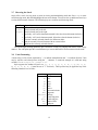
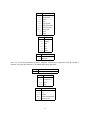
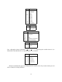
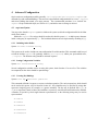
Overview
You can start the calculator by executing orpie. The interface has two panels. The left panel combines
status information with context-sensitive help; the right panel represents the calculator’s stack. (Note that
the left panel will be hidden if Orpie is run in a terminal with less than 80 columns.)
In general, you perform calculations by first entering data on to the stack, then executing functions that
operate on the stack data. As an example, you can hit 1<enter>2<enter>+ in order to add 1 and 2.
3.2
Entering Data
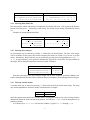
3.2.1 Entering Real Numbers
To enter a real number, just type the desired digits and hit enter. The space bar will begin entry of a scientific
notation exponent. The ’n’ key is used for negation. Here are some examples:
Keypresses
1.23<enter>
1.23<space>23n<enter>
1.23n<space>23<enter>
Resulting Entry
1.23
1.23e-23
-1.23e23
3.2.2 Entering Complex Numbers
Orpie can represent complex numbers using either cartesian (rectangular) or polar coordinates. See Section
3.5 to see how to change the complex number display mode.
A complex number is entered by first pressing ’(’, then entering the real part, then pressing ’,’ followed
by the imaginary part. Alternatively, you can press ’(’ followed by the magnitude, then ’<’ followed by
the phase angle. The angle will be interpreted in degrees or radians, depending on the current setting of the
angle mode (see Section 3.5). Examples:
Keypresses
(1.23, 4.56<enter>
(0.7072<45<enter>
(1.23n,4.56<space>10<enter>
Resulting Entry
(1.23, 4.56)
(0.500065915655126, 0.50006591...
(-1.23, 45600000000)
3.2.3 Entering Matrices
You can enter matrices by pressing ’[’. The elements of the matrix may then be entered as described in the
previous sections, and should be separated using ’,’. To start a new row of the matrix, press ’[’ again. On
the stack, each row of the matrix is enclosed in a set of brackets; for example, the matrix
1 2
3 4
would appear on the stack as [[1, 2][3, 4]].
Examples of matrix entry:
4
Keypresses
[1,2[3,4<enter>
[1.2<space>10,0[3n,5n<enter>
[(1,2,3,4[5,6,7,8<enter>
Resulting Entry
[[1, 2][3, 4]]
[[ 12000000000, 0 ][ -3, -5 ]]
[[ (1, 2), (3, 4) ][ (5, 6), (...
3.2.4 Entering Data With Units
Real and complex scalars and matrices can optionally be labeled with units. After typing in the numeric
portion of the data, press ’ ’ followed by a units string. The format of units strings is described in Section
3.8.
Examples of entering dimensioned data:
Keypresses
1.234 N*mmˆ2/s<enter>
(2.3,5 sˆ-4<enter>
[1,2[3,4 lbf*in<enter>
nm<enter>
Resulting Entry
1.234 N*mmˆ2*sˆ-1
(2.3, 5) sˆ-4
[[ 1, 2 ][ 3, 4 ]] lbf*in
1 nm
3.2.5 Entering Exact Integers
An exact integer may be entered by pressing ’#’ followed by the desired digits. The base of the integer
will be assumed to be the same as the current calculator base mode (see Section 3.5 to see how to set this
mode). Alternatively, the desired base may be specified by pressing space and appending one of {b, o,
d, h}, to represent binary, octal, decimal, or hexadecimal, respectively. On the stack, the representation of
the integer will be changed to match the current base mode. Examples:
Keypresses
#123456<enter>
#ffff<space>h<enter>
#10101n<space>b<enter>
Resulting Entry
# 123456`d
# 65535`d
# -21`d
Note that exact integers may have unlimited length, and the basic arithmetic operations (addition, subtraction, multiplication, division) will be performed using exact arithmetic when both arguments are integers.
3.2.6 Entering Variable Names
A variable name may be entered by pressing ’@’ followed by the desired variable name string. The string
may contain alphanumeric characters, dashes, and underscores. Example:
Keypresses
@myvar
Resulting Entry
@ myvar
Orpie also supports autocompletion of variable names. The help panel displays a list of pre-existing variables
that partially match the name currently being entered. You can press ’<tab>’ to iterate through the list of
matching variables.
As a shortcut, keys <f1>-<f4> will enter the variables (“registers”) @ r01 through @ r04.
5
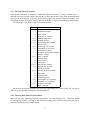
3.2.7 Entering Physical Constants
Orpie includes definitions for a number of fundamental physical constants. To enter a constant, press ’C’,
followed by the first few letters/digits of the constant’s symbol, then hit enter. Orpie offers an autocompletion
feature for physical constants, so you only need to type enough of the constant to identify it uniquely. A list
of matching constants will appear in the left panel of the display, to assist you in finding the desired choice.
The following is a list of Orpie’s physical constant symbols:
Symbol
NA
k
Vm
R
stdT
stdP
sigma
c
eps0
u0
g
G
h
hbar
e
me
mp
alpha
phi
F
Rinf
a0
uB
uN
lam0
f0
lamc
c3
Physical Constant
Avagadro’s number
Boltzmann constant
molar volume
universal gas constant
standard temperature
standard pressure
Stefan-Boltzmann constant
speed of light
permittivity of free space
permeability of free space
acceleration of gravity
Newtonian gravitational constant
Planck’s constant
Dirac’s constant
electron charge
electron mass
proton mass
fine structure constant
magnetic flux quantum
Faraday’s constant
“infinity” Rydberg constant
Bohr radius
Bohr magneton
nuclear magneton
wavelength of a 1eV photon
frequency of a 1eV photon
Compton wavelength
Wien’s constant
All physical constants are defined in the Orpie run-configuration file; consult Section 4 if you wish to
define your own constants or change the existing definitions.
3.2.8 Entering Data With an External Editor
Orpie can also parse input entered via an external editor. You may find this to be a convenient method
for entering large matrices. Pressing ’E’ will launch the external editor, and the various data types may be
entered as illustrated by the examples below:
6
Data Type
exact integer
real number
complex number
real matrix
complex matrix
variable
Sample Input String
#12345678`d, where the trailing letter is one of the base characters {b, o, d, h}
-123.45e67
(1e10, 2) or (1 <90)
[[1, 2][3.1, 4.5e10]]
[[(1, 0), 5][1e10, (2 <90)]]
@myvar
Real and complex numbers and matrices may have units appended; just add a units string such as “ N*m/s”
immediately following the numeric portion of the expression.
Notice that the complex matrix input parser is quite flexible; real and complex matrix elements may be
mixed, and cartesian and polar complex formats may be mixed as well.
Multiple stack entries may be specified in the same file, if they are separated by whitespace. For example,
entering (1, 2) 1.5 into the editor will cause the complex value (1, 2) to be placed on the stack,
followed by the real value 1.5.
The input parser will discard whitespace where possible, so feel free to add any form of whitespace
between matrix rows, matrix elements, real and complex components, etc.
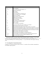
3.3
Executing Basic Function Operations
Once some data has been entered on the stack, you can apply operations to that data. For example, ’+’ will
add the last two elements on the stack. By default, the following keys have been bound to such operations:
Keys
+
*
/
ˆ
n
i
s
a
e
l
c
!
%
S
;
Operations
add last two stack elements
subtract element 1 from element 2
multiply last two stack elements
divide element 2 by element 1
raise element 2 to the power of element 1
negate last element
invert last element
square root function
absolute value function
exponential function
natural logarithm function
complex conjugate function
factorial function
element 2 mod element 1
store element 2 in (variable) element 1
evaluate variable to obtain contents
As a shortcut, function operators will automatically enter any data that you were in the process of
entering. So instead of the sequence 2<enter>2<enter>+, you could type simply 2<enter>2+ and
the second number would be entered before the addition operation is applied.
7
As an additional shortcut, any variable names used as function arguments will be evaluated before application of the function. In other words, it is not necessary to evaluate variables before performing arithmetic
operations on them.
3.4
Executing Function Abbreviations
One could bind nearly all calculator operations to specific keypresses, but this would rapidly get confusing
since the PC keyboard is not labeled as nicely as a calculator keyboard is. For this reason, Orpie includes an
abbreviation syntax.
To activate an abbreviation, press ’’’ (quote key), followed by the first few letters/digits of the abbreviation, then hit enter. Orpie offers an autocompletion feature for abbreviations, so you only need to type
enough of the operation to identify it uniquely. The matching abbreviations will appear in the left panel of
the display, to assist you in finding the appropriate operation.
To avoid interface conflicts, abbreviations may be entered only when the entry buffer (the bottom line of
the screen) is empty.
The following functions are available as abbreviations:
8
Abbreviations
inv
pow
sq
sqrt
abs
exp
ln
10ˆ
log10
conj
sin
cos
tan
sinh
cosh
tanh
asin
acos
atan
asinh
acosh
atanh
re
im
gamma
lngamma
erf
erfc
fact
gcd
lcm
binom
perm
Functions
inverse function
raise element 2 to the power of element 1
square last element
square root function
absolute value function
exponential function
natural logarithm function
base 10 exponential function
base 10 logarithm function
complex conjugate function
sine function
cosine function
tangent function
hyperbolic sine function
hyperbolic cosine function
hyperbolic tangent function
arcsine function
arccosine function
arctangent function
inverse hyperbolic sine function
inverse hyperbolic cosine function
inverse hyperbolic tangent function
real part of complex number
imaginary part of complex number
Euler gamma function
natural log of Euler gamma function
error function
complementary error function
factorial function
greatest common divisor function
least common multiple function
binomial coefficient function
permutation function
9
Abbreviations (con’t)
trans
trace
solvelin
mod
floor
ceil
toint
toreal
add
sub
mult
div
neg
store
eval
purge
total
mean
sumsq
var
varbias
stdev
stdevbias
min
max
utpn
uconvert
ustand
uvalue
Functions
matrix transpose
trace of a matrix
solve a linear system of the form Ax = b
element 2 mod element 1
floor function
ceiling function
convert a real number to an integer type
convert an integer type to a real number
add last two elements
subtract element 1 from element 2
multiply last two elements
divide element 2 by element 1
negate last element
store element 2 in (variable) element 1
evaluate variable to obtain contents
delete a variable
sum the columns of a real matrix
compute the sample means of the columns of a real matrix
sum the squares of the columns of a real matrix
compute the unbiased sample variances of the columns of a real matrix
compute the biased (population) sample variances of the columns of a real matrix
compute the unbiased sample standard deviations of the columns of a real matrix
compute the biased (pop.) sample standard deviations of the columns of a matrix
find the minima of the columns of a real matrix
find the maxima of the columns of a real matrix
compute the upper tail probability of a normal distribution
convert element 2 to an equivalent expression with units matching element 1
convert to equivalent expression using SI standard base units
drop the units of the last element
Entering abbreviations can become tedious when performing repetitive calculations. To save some
keystrokes, Orpie will automatically bind recently-used operations with no prexisting binding to keys <f5>-<f12>.
The current autobindings can be viewed by pressing ’h’ to cycle between the various pages of the help
panel.
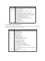
3.5
Executing Basic Command Operations
In addition to the function operations listed in Section 3.3, a number of basic calculator commands have
been bound to single keypresses:
10
Keys
\
|
<pagedown>
<enter>
u
r
p
b
h
v
E
P
C-L
<up>
Q
3.6
Operations
drop last element
clear all stack elements
swap last two elements
duplicate last element (when entry buffer is empty)
undo last operation
toggle angle mode between degrees and radians
toggle complex display mode between rectangular and polar
cycle base display mode between binary, octal, decimal, hex
cycle through multiple help windows
view last stack element in a fullscreen editor
create a new stack element using an external editor
enter π on the stack
refresh the display
begin stack browsing mode
quit Orpie
Executing Command Abbreviations
In addition to the function operations listed in Section 3.4, there are a large number of calculator commands
that have been implemented using the abbreviation syntax:
Abbreviations
drop
clear
swap
dup
undo
rad
deg
rect
polar
bin
oct
dec
hex
view
edit
pi
rand
refresh
about
quit
Calculator Operation
drop last element
clear all stack elements
swap last two elements
duplicate last element
undo last operation
set angle mode to radians
set angle mode to degrees
set complex display mode to rectangular
set complex display mode to polar
set base display mode to binary
set base display mode to octal
set base display mode to decimal
set base display mode to hexidecimal
view last stack element in a fullscreen editor
create a new stack element using an external editor
enter π on the stack
generate a random number between 0 and 1 (uniformly distributed)
refresh the display
display a nifty “About Orpie” screen
quit Orpie
11
3.7
Browsing the Stack
Orpie offers a stack browsing mode to assist in viewing and manipulating stack data. Press <up> to enter
stack browsing mode; this should highlight the last stack element. You can use the up and down arrow keys
to select different stack elements. The following keys are useful in stack browsing mode:
Keys
q
<left>
<right>
r
R
v
E
<enter>
Operations
quit stack browsing mode
scroll selected entry to the left
scroll selected entry to the right
cyclically “roll” stack elements downward, below the selected element (inclusive)
cyclically “roll” stack elements upward, below the selected element (inclusive)
view the currently selected element in a fullscreen editor
edit the currently selected element with an external editor
duplicate the currently selected element
The left and right scrolling option may prove useful for viewing very lengthy stack entries, such as large
matrices. The edit option provides a convenient way to correct data after it has been entered on the stack.
3.8
Units Formatting
A units string is a list of units separated by ’*’ to indicate multiplication and ’/’ to indicate division. Units
may be raised to real-valued powers using the ’ˆ’ character. A contrived example of a valid unit string
would be ”N*nmˆ2*kg/s/inˆ-3*GHzˆ2.34”.
Orpie supports the standard SI prefix set, {y, z, a, f, p, n, u, m, c, d, da, h, k,
M, G, T, P, E, Z, Y} (note the use of ’u’ for micro-). These prefixes may be applied to any of the
following exhaustive sets of units:
String
m
ft
in
yd
mi
pc
AU
Ang
furlong
pt
pica
nmi
lyr
Length Unit
meter
foot
inch
yard
mile
parsec
astronomical unit
angstrom
furlong
PostScript point
PostScript pica
nautical mile
lightyear
12
String
g
lb
oz
slug
lbt
ton
tonl
tonm
ct
gr
Mass Unit
gram
pound mass
ounce
slug
Troy pound
(USA) short ton
(UK) long ton
metric ton
carat
grain
String
s
min
hr
day
yr
Hz
String
K
R
Time Unit
second
minute
hour
day
year
Hertz
Temperature Unit
Kelvin
Rankine
Note: No, Celsius and Fahrenheit will not be supported. Because these temperature units do not share a
common zero point, their behavior is ill-defined under many operations.
String
mol
“Amount of Substance” Unit
Mole
String
N
lbf
dyn
kip
String
J
erg
cal
BTU
eV
Force Unit
Newton
pound force
dyne
kip
Energy Unit
Joule
erg
calorie
british thermal unit
electron volt
13
String
A
C
V
Ohm
F
H
T
G
Wb
Mx
String
W
hp
String
Pa
atm
bar
Ohm
mmHg
inHg
Electrical Unit
Ampere
Coulomb
volt
Ohm
Farad
Henry
Tesla
Gauss
Weber
Maxwell
Power Unit
Watt
horsepower
Pressure Unit
Pascal
atmosphere
bar
Ohm
millimeters of mercury
inches of mercury
String
cd
lm
lx
Luminance Unit
candela
lumen
lux
Note: Although the lumen is defined by 1 lm = 1 cd * sr, Orpie drops the steridian because it is a
dimensionless unit and therefore is of questionable use to a calculator.
String
ozfl
cup
pt
qt
gal
L
Volume Unit
fluid ounce (US)
cup (US)
pint (US)
quart (US)
gallon (US)
liter
All units are defined in the Orpie run-configuration file; consult Section 4 if you wish to define your own
units or change the existing definitions.
14
4 Advanced Configuration
Orpie reads a run-configuration textfile (generally /etc/orpierc or /usr/local/etc/orpierc) to
determine key and command bindings. You can create a personalized configuration file in $HOME/.orpierc,
and select bindings that match your usage patterns. The recommended procedure is to “include” the
orpierc file provided with Orpie (see Section 4.1.1), and add or remove settings as desired.
4.1
orpierc Syntax
You may notice that the orpierc syntax is similar to the syntax used in the configuration file for the Mutt
email client (muttrc).
Within the orpierc file, strings should be enclosed in double quotes ("). A double quote character
inside a string may be represented by \" . The backslash character must be represented by doubling it (\\).
4.1.1 Including Other Rcfiles
Syntax: include filename string
This syntax can be used to include one run-configuration file within another. This command could be used
to load the default orpierc file (probably found in /etc/orpierc) within your personalized rcfile,
˜/.orpierc. The filename string should be enclosed in quotes.
4.1.2 Setting Configuration Variables
Syntax: set variable=value string
Several configuration variables can be set using this syntax; check Section 4.2 to see a list. The variables
are unquoted, but the values should be quoted strings.
4.1.3 Creating Key Bindings
Syntax: bind key identifier operation
This command will bind a keypress to execute a calculator operation. The various operations, which should
not be enclosed in quotes, may be found in Section 4.3. Key identifiers may be specified by strings that
represent a single keypress, for example "m" (quotes included). The key may be prefixed with "\\C" or
"\\M" to represent Control or Meta (Alt) modifiers, respectively; note that the backslash must be doubled.
A number of special keys lack single-character representations, so the following strings may be used to
represent them:
• "<esc>"
• "<tab>"
• "<enter>"
• "<return>"
• "<insert>"
15
• "<home>"
• "<end>"
• "<pageup>"
• "<pagedown>"
• "<space>"
• "<left>"
• "<right>"
• "<up>"
• "<down>"
• "<f1>" to "<f12>"
Due to differences between various terminal emulators, this key identifier syntax may not be adequate to
describe every keypress. As a workaround, Orpie will also accept key identifiers in octal notation. As an
example, you could use \024 (do not enclose it in quotes) to represent Ctrl-T.
Orpie includes a secondary executable, orpie-curses-keys, that prints out the key identifiers associated with keypresses. You may find it useful when customizing orpierc.
Multiple keys may be bound to the same operation, if desired.
4.1.4 Removing Key Bindings
Syntax:
unbind
unbind
unbind
unbind
unbind
unbind
unbind
function key identifier
command key identifier
edit key identifier
browse key identifier
abbrev key identifier
variable key identifier
integer key identifier
These commands will remove key bindings associated with the various entry modes (functions, commands,
editing operations, etc.). The key identifiers should be defined using the syntax described in the previous
section.
4.1.5 Creating Key Auto-Bindings
Syntax: autobind key identifier
In order to make repetitive calculations more pleasant, Orpie offers an automatic key binding feature. When
a function or command is executed using its abbreviation, one of the keys selected by the autobind syntax
will be automatically bound to that operation (unless the operation has already been bound to a key). The
16
current set of autobindings can be viewed in the help panel by executing command cycle help (bound
to ’h’ by default).
The syntax for the key identifiers is provided in the previous section.
4.1.6 Creating Operation Abbreviations
Syntax: abbrev operation abbreviation operation
You can use this syntax to set the abbreviations used within Orpie to represent the various functions and
commands. A list of available operations may be found in Section 4.3. The operation abbreviations should
be quoted strings, for example "sin" or "log".
Orpie performs autocompletion on these abbreviations, allowing you to type usually just a few letters in
order to select the desired command. The order of the autocompletion matches will be the same as the order
in which the abbreviations are registered by the rcfile–so you may wish to place the more commonly used
operation abbreviations earlier in the list.
Multiple abbreviations may be bound to the same operation, if desired.
4.1.7 Removing Operation Abbreviations
Syntax: unabbrev operation abbreviation
This syntax can be used to remove an operation abbreviation. The operation abbreviations should be quoted
strings, as described in the previous section.
4.1.8 Creating Macros
Syntax: macro key identifier macro string
You can use this syntax to cause a single keypress (the key identifier) to be interpreted as the series of
keypresses listed in macro string. The syntax for defining a keypress is the same as that defined in Section
4.1.3. The macro string should be a list of whitespace-separated keypresses, e.g. "2 <return> 2 +"
(including quotes).
This macro syntax provides a way to create small programs; by way of example, the default orpierc file
includes macros for the base 2 logarithm and the binary entropy function (bound to L and H, respectively),
as well as “register” variable shortcuts (<f1> to <f12>).
Macros may call other macros recursively. However, take care that a macro does not call itself recursively; Orpie will not trap the infinite loop.
Note that operation abbreviations may be accessed within macros. For example, macro "A" "’ a
b o u t <return>" would bind A to display the “about Orpie” screen.
4.1.9 Creating Units
Syntax:
base unit unit symbol preferred prefix
unit unit symbol unit definition
Units are defined in a two-step process:
17
1. Define a set of orthogonal “base units.” All other units must be expressible in terms of these base
units. The base units can be given a preferred SI prefix, which will be used whenever the units are
standardized (e.g. via ustand). The unit symbols and preferred prefixes should all be quoted strings;
to prefer no prefix, use the empty string ("").
It is expected that most users will use the fundamental SI units for base units.
2. Define all other units in terms of either base units or previously-defined units. Again, the unit symbol
and unit definition should be quoted strings. The definition should take the form of a numeric value
followed by a units string, e.g. "2.5 kN*m/s". See Section 3.8 for more details on the unit string
format.
4.1.10 Creating Constants
Syntax: constant constant symbol constant definition
This syntax can be used to define a physical constant. Both the constant symbol and definition must
be quoted strings. The constant definition should be a numeric constant followed by a units string e.g.
"1.60217733e-19 C". All units used in the constant definition must already have been defined.
4.2
Configuration Variables
The following configuration variables may be set as described in Section 4.1.2:
• datadir
This variable should be set to the full path of the Orpie data directory, which will contain the calculator
state save file, temporary buffers, etc. The default directory is "˜/.orpie/".
• editor
This variable may be set to the fullscreen editor of your choice. The default value is "vi". It is
recommended that you choose an editor that offers horizontal scrolling in place of word wrapping,
so that the columns of large matrices can be properly aligned. (The Vim editor could be used in this
fashion by setting editor to "vim -c ’set nowrap’".)
• hide help
Set this variable to "true" to hide the left help/status panel, or leave it on the default of "false"
to display the help panel.
• conserve memory
Set this variable to "true" to minimize memory usage, or leave it on the default of "false" to
improve rendering performance. (By default, Orpie caches multiple string representations of all stack
elements. Very large integers in particular require significant computation for string representation,
so caching these strings can make display updates much faster.)
4.3
Calculator Operations
Every calculator operation can be made available to the interface using the syntax described in Sections
4.1.3 and 4.1.6. The following is a list of every available operation.
18
4.3.1 Functions
The following operations are functions–that is, they will consume at least one argument from the stack.
Orpie will generally abort the computation and provide an informative error message if a function cannot be
successfully applied (for example, if you try to compute the transpose of something that is not a matrix).
For the exact integer data type, basic arithmetic operations will yield an exact integer result. Division
of two exact integers will yield the quotient of the division. The more complicated functions will generally
promote the integer to a real number, and as such the arithmetic will no longer be exact.
• function 10 x
Raise 10 to the power of the last stack element (inverse of function log10).
• function abs
Compute the absolute value of the last stack element.
• function acos
Compute the inverse cosine of the last stack element. For real numbers, The result will be provided
either in degrees or radians, depending on the angle mode of the calculator.
• function acosh
Compute the inverse hyperbolic cosine of the last stack element.
• function add
Add last two stack elements.
• function arg
Compute the argument (phase angle of complex number) of the last stack element. The value will be
provided in either degrees or radians, depending on the current angle mode of the calculator.
• function asin
Compute the inverse sine of the last stack element. For real numbers, The result will be provided
either in degrees or radians, depending on the angle mode of the calculator.
• function asinh
Compute the inverse hyperbolic sine of the last stack element.
• function atan
Compute the inverse tangent of the last stack element. For real numbers, The result will be provided
either in degrees or radians, depending on the angle mode of the calculator.
• function atanh
Compute the inverse hyperbolic tangent of the last stack element.
• function binomial coeff
Compute the binomial coefficient (“n choose k”) formed by the last two stack elements. If these
arguments are real, the coefficient is computed using a fast approximation to the log of the gamma
function, and therefore the result is subject to rounding errors. For exact integer arguments, the
coefficient is computed using exact arithmetic; this has the potential to be a slow operation.
• function ceiling
Compute the ceiling of the last stack element.
19
• function convert units
Convert stack element 2 to an equivalent expression in the units of element 1. Element 1 should be
real-valued, and its magnitude will be ignored when computing the conversion.
• function cos
Compute the cosine of the last stack element. If the argument is real, it will be assumed to be either
degrees or radians, depending on the angle mode of the calculator.
• function cosh
Compute the hyperbolic cosine of the last stack element.
• function conj
Compute the complex conjugate of the last stack element.
• function div
Divide element 2 by element 1.
• function erf
Compute the error function of the last stack element.
• function erfc
Compute the complementary error function of the last stack element.
• function eval
Obtain the contents of the variable in the last stack position.
• function exp
Evaluate the exponential function of the last stack element.
• function factorial
Compute the factorial of the last stack element. For a real argument, this is computed using a fast
approximation to the gamma function, and therefore the result may be subject to rounding errors (or
overflow). For an exact integer argument, the factorial is computed using exact arithmetic; this has
the potential to be a slow operation.
• function floor
Compute the floor of the last stack element.
• function gamma
Compute the Euler gamma function of the last stack element.
• function gcd
Compute the greatest common divisor of the last two stack elements. This operation may be applied
only to integer type data.
• function im
Compute the imaginary part of the last stack element.
• function inv
Compute the multiplicative inverse of the last stack element.
20
• function lcm
Compute the least common multiple of the last two stack elements. This operation may be applied
only to integer type data.
• function ln
Compute the natural logarithm of the last stack element.
• function lngamma
Compute the natural logarithm of the Euler gamma function of the last stack element.
• function log10
Compute the base-10 logarithm of the last stack element.
• function maximum
Find the maximum values of each of the columns of a real NxM matrix, returning a 1xM matrix as a
result.
• function minimum
Find the minimum values of each of the columns of a real NxM matrix, returning a 1xM matrix as a
result.
• function mean
Compute the sample means of each of the columns of a real NxM matrix, returning a 1xM matrix as
a result.
• function mod
Compute element 2 mod element 1. This operation can be applied only to integer type data.
• function mult
Multiply last two stack elements.
• function neg
Negate last stack element.
• function permutation
Compute the permutation coefficient determined by the last two stack elements ’n’ and ’k’: the number
of ways of obtaining an ordered subset of k elements from a set of n elements. If these arguments
are real, the coefficient is computed using a fast approximation to the log of the gamma function,
and therefore the result is subject to rounding errors. For exact integer arguments, the coefficient is
computed using exact arithmetic; this has the potential to be a slow operation.
• function pow
Raise element 2 to the power of element 1.
• function purge
Delete the variable in the last stack position.
• function re
Compute the real part of the last stack element.
21
• function sin
Compute the sine of the last stack element. If the argument is real, it will be assumed to be either
degrees or radians, depending on the angle mode of the calculator.
• function sinh
Compute the hyperbolic sine of the last stack element.
• function solve linear
Solve a linear system of the form Ax = b, where A and b are the last two elements on the stack. A must
be a square matrix and b must be a matrix with one column. This function does not compute inv(A),
but obtains the solution by a more efficient LU decomposition method. This function is recommended
over explicitly computing the inverse, especially when solving linear systems with relatively large
dimension or with poorly conditioned matrices.
• function sq
Square the last stack element.
• function sqrt
Compute the square root of the last stack element.
• function standardize units
Convert the last stack element to an equivalent expression using the SI standard base units (kg, m, s,
etc.).
• function stdev unbiased
Compute the unbiased sample standard deviation of each of the columns of a real NxM matrix, returning a 1xM matrix as a result. (Compare to HP48’s sdev function.)
• function stdev biased
Compute the biased (population) sample standard deviation of each of the columns of a real NxM
matrix, returning a 1xM matrix as a result. (Compare to HP48’s psdev function.)
• function store
Store element 2 in (variable) element 1.
• function sub
Subtract element 1 from element 2.
• function sumsq
Sum the squares of each of the columns of a real NxM matrix, returning a 1xM matrix as a result.
• function tan
Compute the tangent of the last stack element. If the argument is real, it will be assumed to be either
degrees or radians, depending on the angle mode of the calculator.
• function tanh
Compute the hyperbolic tangent of the last stack element.
• function to int
Convert a real number to an integer type.
22
• function to real
Convert an integer type to a real number.
• function total
Sum each of the columns of a real NxM matrix, returning a 1xM matrix as a result.
• function trace
Compute the trace of a square matrix.
• function transpose
Compute the matrix transpose of the last stack element.
• function unit value
Drop the units of the last stack element.
• function utpn
Compute the upper tail probability
of a normal
distribution.
R∞ 1
(m−y)2
√
utpn(m, v, x) = x
exp − 2v
dy
2πv
• function var unbiased
Compute the unbiased sample variance of each of the columns of a real NxM matrix, returning a 1xM
matrix as a result. (Compare to HP48’s var function.)
• function var biased
Compute the biased (population) sample variance of each of the columns of a real NxM matrix,
returning a 1xM matrix as a result. (Compare to HP48’s pvar function.)
4.3.2 Commands
The following operations are referred to as commands; they differ from functions because they do not take
an argument. Many calculator interface settings are implemented as commands.
• command about
Display a nifty “about Orpie” credits screen.
• command begin abbrev
Begin entry of an operation abbreviation.
• command begin browsing
Enter stack browsing mode.
• command begin constant
Begin entry of a physical constant.
• command begin variable
Begin entry of a variable name.
• command bin
Set the base of exact integer representation to 2 (binary).
23
• command clear
Clear all elements from the stack.
• command cycle base
Cycle the base of exact integer representation between 2, 8, 10, and 16 (bin, oct, dec, and hex).
• command cycle help
Cycle through multiple help pages. The first page displays commonly used bindings, and the second
page displays the current autobindings.
• command dec
Set the base of exact integer representation to 10 (decimal).
• command deg
Set the angle mode to degrees.
• command drop
Drop the last element off the stack.
• command dup
Duplicate the last stack element.
• command enter pi
Enter π on the stack.
• command hex
Set the base of exact integer representation to 16 (hexadecimal).
• command oct
Set the base of exact integer representation to 8 (octal).
• command polar
Set the complex display mode to polar.
• command rad
Set the angle mode to radians.
• command rand
Generate a random real-valued number between 0 (inclusive) and 1 (exclusive). The deviates are
uniformly distributed.
• command rect
Set the complex display mode to rectangular (cartesian).
• command refresh
Refresh the display.
• command swap
Swap stack elements 1 and 2.
• command quit
Quit Orpie.
24
• command toggle angle mode
Toggle the angle mode between degrees and radians.
• command toggle complex mode
Toggle the complex display mode between rectangular and polar.
• command undo
Undo the last calculator operation.
• command view
View the last stack element in an external fullscreen editor.
• command edit input
Create a new stack element using an external editor.
4.3.3 Edit Operations
The following operations are related to editing during data entry. These commands cannot be made available
as operation abbreviations, since abbreviations are not accessible while entering data. These operations
should be made available as single keypresses using the bind keyword.
• edit angle
Begin entering the phase angle of a complex number. (Orpie will assume the angle is in either degrees
or radians, depending on the current angle mode.)
• edit backspace
Delete the last character entered.
• edit begin integer
Begin entering an exact integer.
• edit begin units
Begin appending units to a numeric expression.
• edit complex
Begin entering a complex number.
• edit enter
Enter the data that is currently being edited.
• edit matrix
Begin entering a matrix, or begin entering the next row of a matrix.
• edit minus
Enter a minus sign in input.
• edit scientific notation base
Begin entering the scientific notation exponent of a real number, or the base of an exact integer.
• edit separator
Begin editing the next element of a complex number or matrix. (This will insert a comma between
elements.)
25
4.3.4 Browsing Operations
The following list of operations is available only in stack browsing mode. As abbreviations are unavailable
while browsing the stack, these operations should be bound to single keypresses using the bind keyword.
• browse echo
Echo the currently selected element to stack level 1.
• browse end
Exit stack browsing mode.
• browse drop
Drop the currently selected stack element.
• browse dropn
Drop all stack elements below the current selection (inclusive).
• browse keep
Drop all stack elements except the current selection. (This is complementary to browse drop.
• browse keepn
Drop all stack elements above the current selection (non-inclusive). (This is complementary to
browse dropn.
• browse next line
Move the selection cursor down one line.
• browse prev line
Move the selection cursor up one line.
• browse rolldown
Cyclically “roll” stack elements downward, below the selected element (inclusive).
• browse rollup
Cyclically “roll” stack elements upward, below the selected element (inclusive) .
• browse scroll left
Scroll the selected element to the left (for viewing very large entries such as matrices).
• browse scroll right
Scroll the selected element to the right.
• browse view
View the currently selected stack element in a fullscreen editor.
• browse edit
Edit the currently selected stack element using an external editor.
26
4.3.5 Abbreviation Entry Operations
The following list of operations is available only while entering a function or command abbreviation, or
while entering a physical constant. These operations must be bound to single keypresses using the bind
keyword.
• abbrev backspace
Delete a character from the abbreviation string.
• abbrev enter
Execute the operation associated with the selected abbreviation.
• abbrev exit
Cancel abbreviation entry.
4.3.6 Variable Entry Operations
The following list of operations is available only while entering a variable name. As abbreviations are
unavailable while entering variables, these operations should be bound to single keypresses using the bind
keyword.
• variable backspace
Delete a character from the variable name.
• variable cancel
Cancel entry of the variable name.
• variable complete
Autocomplete the variable name.
• variable enter
Enter the variable name on the stack.
4.3.7 Integer Entry Operations
The following operation is available only while entering an integer; it can be made accessible by binding it
to a single keypress using the bind keyword.
• integer cancel
Cancel entry of an integer.
5 Licensing
Orpie is Free Software; you can redistribute it and/or modify it under the terms of the GNU General Public
License (GPL), Version 2, as published by the Free Software Foundation. You should have received a copy
of the GPL along with this program, in the file “COPYING”.
27
6 Credits
Orpie includes portions of the ocamlgsl8 bindings supplied by Olivier Andrieu, as well as the curses bindings
from the OCaml Text Mode Kit9 written by Nicolas George. I would like to thank these authors for helping
to make Orpie possible.
7 Contact info
Orpie author: Paul Pelzl <[email protected]>
Orpie website: http://www.eecs.umich.edu/˜pelzlpj/orpie
Feel free to contact me if you have bugs, feature requests, patches, etc. I would also welcome volunteers
interested in packaging Orpie for various platforms.
8
9
http://oandrieu.nerim.net/ocaml/gsl/
http://www.nongnu.org/ocaml-tmk/
28