Download AN ABSTRACT OF THE THESIS OF Thanat Jitpraphai for the

AN ABSTRACT OF THE THESIS OF
Thanat Jitpraphai for the degree of Master of Science in Mechanical Engineering
presented on June 11, 1997. Title: Model Based Visualization of Vibrations in
Mechanical Systems.
Abstract approved:
Redacted for Privacy
Swavik A. Spiewak
To visualize vibrations in mechanical systems, e.g., machine tools, their
movements are measured by means of suitable sensors. The signals from these sensors
are processed and displayed as animated pictures on a computer screen.
Accelerometers have been chosen as the most suitable sensors for this purpose.
Their main advantages include small size, wide sensitivity range and frequency
bandwidth. In addition, accelerometers measure signals with reference to the Earth, so
they do not require stable fixtures such as used with cameras or lasers.
The visualization methodology involves nine accelerometers attached to a
mechanical component, e.g., a dynamometer's platform. Vibration signals were acquired
using a data acquisition (DAQ) system which is controlled by a LabVIEW®-based
program. These signals are processed to suppress errors and convert acceleration into
generalized coordinate that describes motion of the visualized component as a rigid
plate's movement in 3-D space.
The animation is accomplished by displaying a time series of pictures representing
instantaneous position of the plate. The animation program employs homogenous
coordinate transformation to draw 3-D `wireframe' pictures. Since various errors distort
the measured signals, the animated movement may be inaccurate. The knowledge of a
mathematical model of the system whose vibrations are animated allows detection and
suppression of distortions. For this purpose, the signals measured from the actual
dynamic system are compared with the signals simulated by the system's model subjected
to the same excitation as the actual system. Discrepancies between the actual and
simulated signals are detected. They are analyzed to identify possible sources and forms
of distorting signals. As the next step, the measured (actual) signals are corrected by
removing estimated distortions.
A methodology and software package capable of performing all functions
necessary to implement the visualization of vibration have been developed in this
research using LabVIEW® programming environment. As compared with commercial
software for experimental modal analysis, the most distinctive feature of the developed
package is improved accuracy achieved by applying concepts utilized in control theory,
such as modeling of multi-input-multi-output (MIMO) systems and on-line system
identification for the model development and correction of signals.
© Copyright by Thanat Jitpraphai
June 11, 1997
All Rights Reserved
MODEL BASED VISUALIZATION OF VIBRATIONS IN MECHANICAL SYSTEMS
by
Thanat Jitpraphai
A THESIS
submitted to
Oregon State University
in partial fulfillment of
the requirements for the
degree of
Master of Science
Presented June 11, 1997
Commencement June 1998
Master of Science thesis of Thanat Jitpraphai presented on June 11, 1997
APPROVED:
Redacted for Privacy
Major Professor, representing Mechanical Engineering
Redacted for Privacy
Head of Department of Mechanical Engineering
Redacted for Privacy
Dean of Gradu
School
I understand that my thesis will become part of the permanent collection of Oregon State
University libraries. My signature below authorizes release of my thesis to any reader
upon request.
Redacted for Privacy
Thanat Jitpraphai, Author
ACKNOWLEDGMENT
I would like to express my appreciation to my advisor, Dr. Swavik A. Spiewak. I
first met Professor Spiewak in his Smart Product and Design class where he showed me
the power of computer programs (that have leaded to the LabVIEW® programs in this
thesis). Without the inspiration as well as his advice, encouragement and great effort, this
thesis would not have been accomplished. I would also like to thank the students in my
research group, Thomas Nickel, Brian Brisbine, Ben Chen and all of my friends in
helping me out of many difficulties.
I would like to thank sincerely to my parents, Dr. Phaibul and Dr. Chattaya
Jitpraphai as well as my brothers, Peera and Siros, for their encouragement and support
for my study.
I would like to thank to my special person, Waranush Sorasuchart, for her care
and patience during this work. Thanks also due to all of my Thai-OSU friends who help
me in many things.
TABLE OF CONTENTS
Page
CHAPTER 1
INTRODUCTION
1
1.1 Graphical Representation of Vibration
1
1.2 Scope of Work
2
1.3 Chapter Overview
3
CHAPTER 2
LITERATURE REVIEW
4
2.1 Visualization in Vibration Analysis
4
2.2 System Identification in Vibration Analysis
7
2.3 Conventional Visualization Software
10
2.4 Measurement of Signals for Visualization
12
2.4.1 Piezoelectric Accelerometer Measurement
13
2.4.2 Conventional Low Frequency Accelerometers
20
2.4.3 Multi Directional Accelerometer
24
2.5 Closure
25
CHAPTER 3
MODEL BASED VISUALIZATION OF VIBRATIONS
26
3.1 An Overview and Definition of the Proposed Visualization Technique
26
3.2 Signal Based Vibration Visualization
28
3.3 Model Based Vibration Visualization
29
3.4 Feasibility Study of the Visualization Enhancement
35
TABLE OF CONTENTS (Continued)
Page
3.5 Modeling of the Dynamometer
37
3.5.1 Mechanistic Model
39
3.5.2 State Space Model
41
3.5.3 Transfer Function Model
43
3.6 Closure
44
CHAPTER 4
THE SIGNAL BASED VIBRATION VISUALIZATION
45
4.1 Visualization of Machine Vibrations
45
4.1.1 Overview of the Methodology
46
4.1.2 Introduction to LabVIEW® Programming Environment
48
4.2 Data Acquisition System Used in Vibration Visualization
52
4.2.1 Anti-aliasing Filtering
53
4.2.2 Attenuation of Noise in a Data Acquisition
53
4.2.3 Data Acquisition Program
55
4.3 Signal Processing in Vibration Visualization
55
4.3.1 Conversion to Physical Units and Subtraction of the
Average Value
56
4.3.2 High-pass Filtering and Double Integration Procedure
57
4.4 Coordinate Systems
59
4.5 Calculation of the Generalized Coordinates from Experimental Data
61
4.6 Animation of the Rigid Body Motion
64
4.6.1 Finding Absolute Position of the Reference Corner Point
65
4.6.2 Calculating Coordinates of the Plate Corners
66
4.6.3 Projection of 3-D Object to a Planer (2-D Screen)
71
4.6.4 Changing the Viewpoint
73
4.6.5 Drawing a Single 3-D Picture
75
TABLE OF CONTENTS (Continued)
Page
4.6.6 Animation of Generated 3-D Pictures
76
4.7 Transformation of Generalized Coordinates in a Rigid Plate
78
4.8 Closure
79
CHAPTER 5
EXPERIMENTAL IMPLEMENTATION AND RESULTS
80
5.1 Experimental Set Up
80
5.2 Data Acquisition and Vibration Visualization Software
84
5.3 Verification of the Developed Software Modules
87
5.3.1 Experimental Procedure
87
5.3.2 Results and Discussion
88
5.4 Comparison of Signal Based and Model Based Responses
91
5.4.1 Experimental Procedure
91
5.4.2 Results and Discussion
92
5.5 Closure
99
CHAPTER 6
CONCLUSIONS AND RECOMMENDATIONS
100
6.1 Conclusions
100
6.2 Recommendations
101
BIBLIOGRAPHY
103
APPENDICES
107
LIST OF FIGURES
Page
Figure
2.1
Equivalent forms of a mechanical model used in vibration analysis
5
2.2
A 2-DOF model of an automobile
6
2.3
Vibrating lumped system in two different mode shapes
7
2.4
Obtaining the system's model by means of an identification procedure
8
2.5
Classification of the system identification techniques
9
2.6
Parametric identification
10
2.7
An animation of vibration on the display of ME ScopeTM
11
2.8
Six coordinates describing motion of a rigid plate
12
2.9
Configurations of piezoelectric accelerometers including
(a) compression type and (b) shear type
14
2.10
Comparison diagrams of instrument setup between the high and low
impedance system
15
2.11
Cross-section diagram of the ICP accelerometer
16
2.12
Magnitude plot of the FRF of a piezoelectric accelerometer
17
2.13
Illustration of the impact of a low frequency drift on the displacement
obtained from acceleration signal
20
2.14
Signals obtained by means of a variable capacitance accelerometer
and its results from double-integration
22
2.15
Schematic illustration of a single-element electron tunneling accelerometer
23
2.16
A cross section of a piezoresistive accelerometer
24
2.17
A cross section of the PiezoBEAM® accelerometer
24
3.1
Flowchart of model based visualization of vibrations
27
3.2
A flowchart representation of the methodology developed for the signal based
vibration visualization
28
3.3
Classification of dynamic systems
29
3.4
The MIMO system
30
3.5
Block diagram of the model based vibration visualization
32
3.6
Block diagram of the Comparison and Correction
33
3.7
An alternative flowchart of the model based vibration visualization
35
LIST OF FIGURES (Continued)
Figure
Page
3.8
Major components of the dynamometer
36
3.9
Main research subjects pertaining to model based visualization
37
3.10
A high speed machine tool
38
3.11
A simplified model of the machine tool from Fig. 3.10 with the
dynamometer installed
38
3.12
Simplified mechanical model of the dynamometer under consideration
40
4.1
Components of the generalized coordinate list, dG, describing
the 'rigid-body' motion of a plate
46
4.2
Flowchart of the methodology used for the visualization of machine
vibrations
47
4.3
An example program (virtual instrument) in LabVlEW®
49
4.4
Front panels of LabVIEW® programs developed for the vibration visualization 50
4.5
A block diagram of the basic data acquisition system used in this research
52
4.6
A flowchart of signal processing in vibration visualization
55
4.7
Diagram of the signal processing procedure
59
4.8
Coordinate systems used in describing the plate motion
60
4.9
Locations of nine accelerometers required for the calculation of
the generalized coordinates
63
4.10
A flowchart of the procedure calculating the list of absolute generalized
coordinates
66
4.11
Abbrevations used to designate the plate's corner
67
4.12
Definition of coordinate transformation matrices
69
4.13
Application of the homogeneous coordinate transformation for finding
coordinates of point A
70
4.14
Flowchart shows procedure of calculating coordinates of all corners
72
4.15
Illustration of the projection of a 3-D object on a 2-D planer
73
4.16
Illustration of the effect from changing the viewpoint on the 2-D picture
74
4.17
Diagram of coordinate transformation procedure for changing the viewpoint
75
4.18
A flowchart of the entire animation procedures
77
LIST OF FIGURES (Continued)
Page
Figure
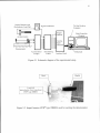
5.1
Schematic diagram of the experimental setup
81
5.2
Impact hammer (PCB® type 208B03) used for exciting the dynamometer
81
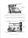
5.3
Locations of nine accelerometers (Kistler® type 8702B25M1) mounted
on the dynamometer
83
5.4
The data acquisition system
83
5.5
Icons and wiring terminals of the major LabVIEW® modules employed
in the vibration visualization
84
5.6
A simplified diagram of the LabVIEW® visualization programs
using modules shown in Fig. 5.5
86
5.7
Definitions of characteristic time instances referred to Table 5.1 and 5.2
89
5.8
Graphs show results from the test number 5
93
5.9
Graphs show results from the test number 6
94
5.10
Graphs show results from the test number 7
95
5.11
Graphs show results from the test number 8
96
5.12
Illustration of the flexible mode of platform's vibration
from the test number 5
98
LIST OF TABLES
Page
Table
2.1
Effect of time constant on the error in measuring various transient responses
4.1
Coordinates of the corners and equations used for calculations
67
4.2
Order of corner plotting for creating a complete 3-D rectangular plate
76
5.1
Descriptions of the test procedures used in the experiment
88
5.2
Characteristic locations of the dynamometer's platform
obtained experimentally
90
5.3
Description of procedures in the experiment
92
.. 18
LIST OF APPENDICES
Page
Appendix A
Experiment Specifications
108
Appendix B
Parameters of the Dynamometer's Model
110
Appendix C
MATLAB® Program Used in the Experiment
112
Appendix D
Descriptions of the LabVIEW® Visualization Programs
118
Appendix E Data Management in the LabVIEW® Visualization Programs
127
Appendix F
132
Block Diagrams of the LabVIEW® Visualization Programs
LIST OF APPENDIX FIGURES
Figure
Page
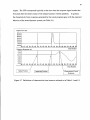
A.1
Power spectrum density of signal measured from an accelerometer
108
A.2
Dimensions of the dynamometer used in the experiment in units of mm
(the sensing elements are not shown)
109
A.3
Digital high-pass filter's coefficients used in Eq. 4.4 and 4.6
109
D.1
Front panel of Data Acquisition Controller program (DAC)
118
D.2
Front panel of the signal processor program (SP)
120
D.3
Front panel of the generalized coordinate calculator program (GCC)
122
D.4
Front panel of the 3-D animation generator program (AG)
123
D.5
Dimensions used in the 'center reference' drawing option
125
D.6
Dimensions used in the 'corner reference' drawing option
126
E.1
Data system
127
LIST OF APPENDIX TABLES
Page
A.1
Descriptions of sensors used in the experiment
108
E.1
Formats of data used in the visualization programs
128
E.2
Systeminfo assignment
129
E.3
Example of the Systeminfo file used in the experiment
131
LIST OF ABBREVIATIONS
C.S.
= Coordinate System
CFR = Characteristic Forced Response
DAQ = Data Acquisition
EMA = Experimental Modal Analysis
FLL
= Front Left Lower Corner
FLU
= Front Left Upper Corner
FRF
= Frequency Response Function
FRL
= Front Right Lower Corner
FRU = Front Right Upper Corner
G
= Graphical Programming Language
ICP
= Integrated Circuit Piezoelectric
IIR
= Infinite Impulse Response
MBR = Model Based Response
MDOF = Multi Degree of Freedom
MIMO = Multi Input Multi Output
N-DOF = N Degrees of Freedom
ODS = Operational Deflection Shape
RLL = Rear Left Lower Corner
RLU = Rear Left Upper Corner
RRL = Rear Right Lower Corner
RRU = Rear Right Upper Corner
SBR = Signal Based Response
SISO = Single Input Single Output
VI
= Virtual Instrument
NOMENCLATURE
(XYZ) = global coordinate system comprises of X, Y and Z axes
(XYZ), = coordinate system at the plate's center of mass comprises of XG, Y, and ZG axes
(XYZ), = instantaneous coordinate system of the plate comprises of X Y, and Z, axes
(XYZ)R = reference coordinate system of the plate comprises of XR, YR and Z axes
(XYZ), = viewpoint coordinate system of the plate comprises of Xi Y. and 4 axes
A, B, C, D = coefficient matrices of state space equations
AG
= "3-D Animation Generator.VI" LabVIEW® program
A,
= amplitude of acceleration applied to an accelerometer
a a,, = accelerations of point C and P, respectively, in (XYZ),,
al
= acceleration in i direction at corner j; i = x, y and z; j = C, 1, 2, and 3
a, ay, a,
= distances between the force application point and G in the XG, Y, and ZG
directions, respectively
c
= damping coefficient
c
= damping matrix of the spatial model
C
= origin of (XYZ),
CR
= origin of (XYZ),,
Cu
= constant matrix converting actual input u into Fe
D12
= 1x4 matrix describes a vector from point 1 to point 2
DAC = "Data Acquisition Controller.VI" LabVIEW® program
dc, dp = generalized coordinates of point C and P, respectively, with respect to (XYZ)
d,
= generalized coordinate of point C with respect to (XYZ),,
d.
= generalized coordinate of point CR with respect to (XYZ)
= vector of translational motion of the dynamometer's base
F
= vector of the forces acting on the dynamometer's platform
Fe
= vector of the forcing function acting on the platform's center of mass
F,
= components of the force vector, i = x, y and z
Fr
= vector of the measured force signal
= Nyquist frequency
fm
f
G
= measurement frequency bandwidth of the piezoelectric accelerometer
= sampling frequency
= center of mass
GCC = "Generalized Coordinate Calculator.VI" LabVIEW® program
GE(s) = transfer function matrix of the equivalent system
Gf
= gain of the amplifier in the anti-aliasing filter
G,(s) = element of the transfer function matrix Gs(s)
Gs(s)
= transfer function matrix of the system
= FRF of the low impedance piezoelectric accelerometer system
= rotational magnification factor
H,
= translational magnification factor
= n by n identity matrix
i
= index denoting the direction
i0, j0, kG = unit vectors in X0, YG and ZG axes, respectively
i,, j,, k, = unit vectors in X Y, and Z, axes, respectively
J
j
= mass moment of inertia
= index denoting the corners of the plate
k, k,, k2 = stiffness coefficient
k
= stiffness matrix of the spatial model
kA
= conversion factor
1, w, h = dimensions of the plate in X,, Y, and Z, directions
14
= length of the automobile model
/G, wG, hG = distances from point C to point G in X Y, and Z, directions
1,, w0, ho = distances from point 0 to point C in X, Y and Z directions
m
= mass
m
= mass matrix of the spatial model
M
= vector of torques acting on the dynamometer's platform
M,
= moment acting on the dynamometer's platform; i = x, y and z
= moment caused by the force F acting away from G; i = x, y and z
NF, NR = number of the forward and reverse coefficients, respectively
O
= origin of the (XYZ)
0. = n by n zero matrix
P
= arbitrary point on a rigid plate
q(t)
= vector of state variable
Q(s)
= Laplace transform of q(t)
r
= position vector of point P from point C
r, r rz= distances between accelerometers
1?,
= kth reverse coefficient of the digital filter
12,
= rotational motion of the dynamometer's base
s
= Laplace variable
SP
= "Signal Processor.VI" LabVIEW® program
SPF
= signal processing function
s,,
= accelerometer sensitivity
T,2
= homogeneous transformation matrix from C.S.1 to C.S.2
t,
= measuring time of the transient response of the piezoelectric accelerometer
TC
= time constant of the miniature amplifier in the transducer
TC1
= time constant of the power supply
U(s)
= Laplace transform of the input u(t)
u(t)
= input vector
U,,,(s)
= Laplace transform of the measured input um(t)
um(t)
= measured input signal
V,
= amplifier output voltage
Vr
= voltage signal recorded by the data acquisition program
x' , y', z' = coordinates in a different coordinate system
x1[n]
= nth element of a sequence of the discrete acceleration signal
x2[n]
= nth element of a sequence of the discrete filtered acceleration signal
x.,[n]
= nth element of a sequence of the discrete velocity signal
xi[n]
= nth element of a sequence of the discrete filtered velocity signal
x s[n]
= nth element of a sequence of the discrete displacement signal
x, y, z = translations of point G relatively to point 0, parallel to X, Y and Z axes
xc, yc, zc = translations of point C relatively to point 0, parallel to X, Y and Z axes
yG, zG
= translations of point G relatively to point 0, parallel to X, Y and Z axes
x y z, = translations of point C relatively to point CR, parallel to XR, YR and ZR axes
XT, 17, ZT
= translations of the dynamometer's base in X, Y and Z directions
Y(s)
= Laplace transform of the output y(t)
y(t)
= output vector
yE(t)
= estimated output vector from GE(s) and U(s)
Z
= amplitude of the automobile's translation
a
= angular acceleration of point P in (XYZ),
a,
= angular accelerometer component of the vector a ; i = x, y and z
At
= sampling period
O
= amplitude of the automobile's rotation
0, 0, 1/1 = rotations of C.S. (XYZ)G around X, Y and Z axes, respectively
0c, 0c, v' = rotations of C.S.(XYZ), around X, Y and Z axes, respectively
0
= rotations of C.S.(XYZ), around XR, Y and ZR axes, respectively
= rotations of C.S.(XYZ), around X, Y and Z axes, respectively
er Or yi, = rotations of the dynamometer's base around X, Y and Z axes, respectively
ev, 0v, yiv = rotations of C.S.(XYZ), around X, Y and Z axes, respectively
= angular velocity of point P in C.S.(XYZ),
ZiT
= angular velocity component of the vector W; i = x, y and z
co
= frequency variable
co
con
coz
= natural frequency of an example automobile
= natural frequency
= low and high limits of the measuring frequency of the accelerometer
Ni
= mode shape
= damping coefficient
MODEL BASED VISUALIZATION OF VIBRATIONS
IN MECHANICAL SYSTEMS
CHAPTER 1
INTRODUCTION
1.1 Graphical Representation of Vibration
Graphical representation of vibration aids engineers in analysis of dynamic
behavior of mechanical systems. Analysts have better understanding of vibration
problems by looking at actual movement of components under consideration. Unlike the
vibration analysis based on the finite element method and modal analysis software, the
visualization of the actual movement can provide information that is often beyond the
estimated display generated by the analytical methods.
The visualization of actual vibrations in mechanical systems is accomplished by
measuring the movement of these systems with suitable sensors. Signals from these
sensors are processed and displayed as graphical representation of the vibration. To
measure signals required for the visualization, many different methods have been
developed, such as laser beam scanning schemes, fiber optics based sensors, vision
systems, or magnetic sensors. The application of these systems is costly and therefore
limited. Accelerometers, on the other hand, are effective with reasonable cost. They also
provide advantages including small size, wide sensitivity range and frequency bandwidth.
In addition, accelerometers measure the signals with reference to the Earth, so they do not
require stable fixtures such as used with cameras or lasers. Therefore, the accelerometers
have been chosen as the most suitable sensors in this research.
Algorithms have been developed and implemented as programs for the
visualization purpose. In the course of this project numerous problems have emerged
2
associated with the use of accelerometers. These problems centered around errors in
measured signals. These errors were attributed either to the environment or
characteristics of the sensors themselves. A suitable method for suppressing the errors
has been proposed in this research.
Despite the precautions taken to suppress errors in the signals used for
visualization there is no guarantee that the displayed motion accurately represents the
actual behavior of tested system. To improve the reliability of visualization a
methodology have been proposed that allows the detection and correction of errors. This
methodology involves concepts developed in control theory as well as analytical models
of systems whose vibrations are visualized.
1.2 Scope of Work
The research discussed in this thesis addresses two major areas and has two
objectives. The first objective is the development of a visualization program capable of
acquiring acceleration signals that represent vibrations. These signals are processed to
obtain three-dimensional movements of mechanical systems and displayed as graphical
animation representing the vibrations. This objective is accomplished and presented in
this thesis.
The second objective is an enhancement of the above visualization program by
utilizing information encapsulated in analytical models of investigated systems to detect
and eliminate errors of visualization. The work in this area is only outlined here and
recommended as the future development. However, a preliminary experiment was
conducted in this thesis to study the feasibility of using analytical models for the purpose
of visualization enhancement.
3
The visualization technique and software developed in the thesis apply to a rigid
body motion. In particular, the motion of a plate suspended on four three-dimensional
springs is investigated. This plate is one component of a multi-component force sensor
(dynamometer). A model of this dynamometer is known from previous research (Chung,
1993; Chen, 1996) and is ready to be used in a comparative experiment for the feasibility
study of the model based enhancement of visualization.
1.3 Chapter Overview
Visualization by means of vibration analysis is introduced in Chapter 2. System
identification technique is also described since it will be used as part of the model
development necessary for enhancing the visualization program. Basics of piezoelectric
accelerometers dealt within this research are reviewed with respect to their applications
and possible errors resulted from their characteristics. Alternative accelerometers are
discussed as a suggestion for the research improvement.
In Chapter 3, a concept of the model based enhancement of visualization is
introduced. A terminology used in the research is defined at the beginning of the chapter
followed by a brief explanation of a methodology of the visualization. Possible extension
of work is also delineated. Finally, the mathematical model of a dynamometer employed
from previous researches is discussed as this model underlines the proposed extension of
work.
In Chapter 4 theory and algorithms used in the visualization program developed in
this thesis is explained. Experiments conducted for the program verification are
described with results and discussion in Chapter 5. The experiments also involve a
comparison between results from the visualization program and those from the
mathematical model. Finally, conclusions and a future direction of the research are stated
in Chapter 6.
4
CHAPTER 2
LITERATURE REVIEW
The objectives and application of vibration analysis are discussed and a
motivation for the visualization of vibration is presented. System identification
techniques as an enhancement of the vibration analysis are also reviewed. Representative
visualization techniques and commercial programs are briefly characterized followed by
an introductory discussion of the proposed visualization technique. Since piezoelectric
accelerometers have been used to measure vibrations of system in this research, the
design and performance of these accelerometers is described. Finally, the latest advances
in relevant sensor technology, i.e., low frequency accelerometers and multi directional
sensors, are reviewed.
2.1 Visualization in Vibration Analysis
Vibration analysis is a study of dynamic behavior of a system. As a rule, the
analysis involves an attempt to define mechanical systems by means of mathematical
models. The systems are usually described by one of the following model forms: a spatial
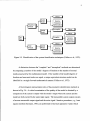
model, a modal model, and a response model (Ewins, 1984). These three forms are
related to each other and one form can be transformed into another as shown in Fig. 2.1.
The spatial model describes the system based on its physical parameters,
including masses (m), stiffness (k) and damping coefficients (c). These properties are
usually formed in the equation of motion. The modal model is obtained by applying 'free
vibration analysis' to the spatial model which results in the information given by a set of
natural frequencies (con), damping ratios (4), and corresponding mode shapes (w).
5
Spatial Form
Parameters:
Mass
Damping
Stiffness k
Response Form
Modal Form
Parameters:
Frequency Response
Function (FRF)
Parameters:
Natural frequencies CO
Mode shapes
yr
Damping ratio
Figure 2.1 Equivalent forms of a mathematical model used in vibration analysis.
By applying 'forced vibration analysis' to either the modal or the spatial model, a
response model is obtained. This model describes the response of the system when
exposed to an external excitation. The response is usually expressed in a standard form
as the system's response to a unit-amplitude sinusoidal force applied to each point on the
system individually and at every frequency within a specified range. Therefore, the
response model consists of a set of frequency response functions, FRFs (Ewins, 1984).
In the visualization aspect, the vibration analysis is applied, obtained and
interpreted the movements of an excited system. The motion of a system usually does not
occur in one direction, but involves various translations, rotations, as well as deflection.
Such motion is referred to as having more than one degree of freedom.
A multi degree of freedom system (MDOF) requires more than one coordinate to
describe its dynamic motion. If a system requires N coordinates to characterize its motion
such the system is termed N degrees of freedom system, or briefly an N-DOF system.
Mode shape (N') is a set of relative amplitudes of the coordinates at certain
frequency of vibration. It describes how one coordinate behaves relatively to the others.
6
An N-DOF system has N natural frequencies with N corresponding mode shapes
(Thomson, 1993).
An example of the mode shape representation applied to an automobile is shown
in Fig. 2.2.
Equilibrium position
k1(z - 11 sin(0 ))
(a) Lumped parameter system.
k2(z + 12 sin(0 ))
(b) Free body diagram.
Figure 2.2 A 2-DOF model of an automobile (Thomson, 1993).
The automobile's dynamics is simplified such that it can be described by a lumped
mass that moves only in a vertical direction and rotates around its center of mass.
Therefore, this simplified automobile requires two coordinates, z and a to described its
motion (or it has two degrees of freedom, 2 -DOF).
To define z and 0 coordinates completely, reference axis of position and
orientation is required. As shown in Fig. 2.2b, the system is reduced to a free body
diagram (FBD) in which only external forces are concerned. The reference point is
chosen at the center of mass. Any vertical translation from the reference position is
described by z and a rotation around the center of mass is defined by 0 as shown in the
FBD.
To illustrate the mode shape, constant parameters are chosen to represent the
automobile's properties. These parameters include m = 3220 lb., k1= 2400 lb./ft, k2 =
7
2600 lb./ft, /I = 4.5 ft, /2 = 5.5 ft, and J = 51520 lb.ft2. By assuming that the responses of
the model have the forms: z(t) = Zei" and 0 (t) = 0e'" , the natural frequencies are
calculated as co, = 6.90 rad/sec and (02= 9.06 rad/sec. The corresponding mode shapes are
calculated (Thomson, 1993).
1V1 = {
Z/
1-1.091
le
1
= i
1
1
1
1
2
(2.1)
f
The mode shapes can be symbolically represented as shown in Fig. 2.3.
= 6.90 rad/s
co2 = 9.06 rad/s
Nodeldi
Node
k2
//11//1/1
14.6 ft
(a) Vibration at co, and
1.09 ft
(b) Vibration at cwt and V2.
Figure 2.3 Vibrating lumped system in two different mode shapes (Thomson, 1993).
2.2 System Identification in Vibration Analysis
Theoretically estimated parameters (m, c, k) in the model are usually not adequate
to describe an actual system. Some parameters are difficult to identify such as the
damping coefficients and stiffness of the system. An efficient method is required to
estimate the model parameters which are as close to the actual system as possible.
System identification provides means to obtain such parameters for the purpose of
developing mathematical models which describe the static and dynamic behavior of
systems in a sufficiently accurate manner (Unbehauen, 1982). In system identification a
model equivalent of the system of interest is determined based upon an input and an
output of the system as shown in Fig. 2.4 (Natke, 1982).
8
Excitation
Physical System
Response
Identification
Procedure
Input
The System's
Model
Output
Figure 2.4 Obtaining the system's model by means of an identification procedure (Natke,
1982).
Algorithms used in the system identification can be classified as shown in Fig. 2.5.
Mainly, determination of the model can be performed either in the frequency domain or in
the time domain. In the frequency domain, the estimation of model parameters is based on
fitting the model frequency response to the measured frequency response of the system. In
the time domain approach the estimate of system parameters are based directly on the
measured system's excitations and responses (Collins et. al., 1972).
The methods are also classified based on the spatial model or the modal model.
Both approaches govern either one or both techniques: direct or iterative schemes. The
"direct" or non-parametric identification approach is based on developing a single step
solution procedure that estimates all required parameters. The "iterative parameter
optimization" or parametric identification is based on the use of algorithms that relate
change in parameter values to change in model responses in which a priori knowledge of
the system is required to derive a mathematical model (Collins et al., 1972).
9
Direct
Modal
0,Model
Frequency
--1 Domain
Spatial
Model
Iterative
Parameter
Optimization
Incomplete
1_4,
Direct
_0[Complete
Test
Data
Direct
Time
Domain
Spatial
Model
Direct
I
Iterative
Parameter
Optimization
Iterative
Parameter
Optimization
Figure 2.5 Classification of the system identification techniques (Collins et. al., 1972).
A distinction between the "complete" and "incomplete" methods are determined
by comparing a number of the model's degrees of freedom to the number of normal
modes possessed by the mathematical model. If the number of the model degrees of
freedom and measured modes are equal, a unique equivalent structure model can be
identified in a straight forward mathematical manner (Collins et al., 1972).
A block diagram representation idea of the parametric identification methods is
shown in Fig. 2.6. A critical examination of the quality of the model is obtained by a
comparison of the system's output with the model's output where the system and the
model are both excited by the same input signal. The measurable system output consists
of an non-measurable output signal and the noise signal. Iterative procedures, e.g., least
squares method (Isermann, 1981), are performed to find such parameter values which
10
yield the error between the model output and the system output as small as possible
(Unbehauen, 1982).
Input Signal
System
Model
Non-measurable
Output Signal
Noise Signal
System Output
Output of the Model
Error
Parameter Values
Parameter Adjustment and
Adaptation Algorithm
Figure 2.6 Parametric Identification (Unbehauen, 1982).
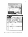
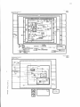
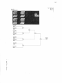
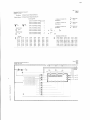
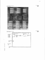
2.3 Commercial Visualization Software
The majority of commercial programs in vibration analysis visualize vibrations in
mechanical systems by presenting the mode shapes of investigated system. These mode
shapes are calculated either from an analytical approach or an experiment. In practical
experimental modal analysis (EMA) software generates the mode shapes from a transfer
function calculated using data from an experiment. Once the transfer function of the
system of interest is obtained (based on the input and output signals), the natural
frequencies and corresponding mode shapes are determined (Powell, 1992).
The vibration is presented as a relative movement of one part of the system with
respect to the others. For example, if a user decomposes the visualized system into a
sufficient number of elements, each point or node is assigned to represent the vibration of
that particular element. In the animation of vibration, one reference node is displayed as
oscillating sinusoidal with corresponds to a forced harmonic FRF responses at the selected
resonance frequency. Positions of the other nodes are then calculated by using the relative
11
displacement information provided in the identified mode shapes. Therefore, the graphical
display shows vibrating shape or deflected shape of the system at this selected resonance
frequency (Vibrant Technology, 1996). An example of visualization display presenting
mode shape of a plate at a certain frequency is illustrated in Fig. 2.8. Available software in
the EMA area are LMS CADA -XTM, STAR systemTM, EMODALTM, I- DEASTM, PC
MODALTM, and ME ScopeTM (Lang, 1990; Spectral Dynamics, 1995; Structural Dynamics
Research Corporation, 1996; Vibration Engineering Consultants, 1997).
Animate: PLT MODE S.STR - Mode#01-340.000 Hz Orr
Pr
-Lesiakcii
Moden1-340.0130 Hz
FP FP T
1111 112/2522. G. / IIi
1=111
0
JP
1.71
0
11
lir IF
712.11111,.1.
112/2722. G. 114
41.21 I
44.7
24.7
JP
4.72
X
15.2
1 11
1
251
.411e752.111Uppla
511
751
1.111
Figure 2.7 An animation of vibration on the display of ME ScopeTM (Vibrant Technology,
1996).
Another approach to visualize vibrations in commercial software is to display the
operational deflection shape (ODS) in which the forced dynamic deflection is determined
at the operating frequency (Powell, 1992). This technique is utilized to find the mode
shape of the system directly from an experiment. By mounting sensors (usually
accelerometers) at specified nodes on the system's surfaces and then exciting the system
with a suitable excitation, the relative deflection of each node is obtained by capturing all
12
signals from all nodes simultaneously when the system is subjected to excitation (Powell,
1992).
2.4 Measurement of Signals for Visualization
An approach of visualization technique in this research is similar to the
Operational deflection Shape technique discussed above. Vibration of the system under
consideration are measured in actual operating conditions using suitable sensors and then
displayed directly. Therefore, this visualization method presents the actual movement of
the system.
The technique proposed in this research is explained by way of example. A rigid
plate fixed with springs and dampers represents a mechanical system. To visualize the
complete motion of the plate six coordinates are required, which include three for
rotations and three for translations. Discussion of these coordinates follows.
z
Figure 2.8 Six coordinates describing motion of a rigid plate.
13
The plate under investigation is shown in Fig. 2.8 in the Cartesian coordinate
system comprising three orthogonal axes XG, YG, and ZG, defining a plate coordinate
system (XYZ)G. The origin of (XYZ)G is the center of mass of the plate, G. Another
coordinate system (XYZ), composed of three perpendicular axes, X, Y, Z, is introduced as
a global reference coordinate system. When the (XYZ) is fixed with reference to the
Earth, a motion of the plate can be described as a relative movement between the (XYZ)G
and the (XYZ). Variables required for describing this motion are:
x - the translation of point G relatively to point 0, parallel to the axis X,
y
the translation of point G relatively to point 0, parallel to the axis Y,
z
the translation of point G relatively to point 0, parallel to the axis Z,
0
the rotation of the plate around the X axis (roll angle),
0 - the rotation of the plate around the Y axis (pitch angle), and
tit
the rotation of the plate around the Z axis (yaw angle).
Linear accelerometers are employed in this research to detect linear vibration of
the specific points of the plate in the X, Y and Z directions. The rotations are indirectly
calculated from these linear accelerations using a technique proposed by Padgaonkar et al.
(1975). This technique is further described in Section 4.5.
Piezoelectric accelerometers have been chosen because of their reasonable cost
and excellent performance. However, the piezoelectric sensors are charge generators that
require special amplifiers. Without proper amplifiers, these sensors can significantly
distort the motion measurement. Details are discussed in the following section.
2.4.1 Piezoelectric Accelerometer Measurement
Piezoelectric transducers utilize piezoelectric effects occurring in certain crystals.
The deformations of these crystals, due to an applied pressure, produce electrical charges
on the external crystal surfaces. These effects occur in materials such as single-crystal
14
quartz, polycrystalline barium titanate, or lead zirconate (Kial and Mahr, 1984). A
piezoelectric accelerometer consists of a piezoelectric sensing element sandwiched
between the transducer's body and a seismic mass, as shown in Fig. 2.9. By mounting the
transducer on a surface of a vibrating object, internal forces from the seismic mass cause
deformations in the sensing element which, in term, produce an electrical charge (Da lly et
al., 1993).
Cover
Center Post
Nut
Cover
Seismic Mass
Piezoelectric
Element
Base
Threaded Hole for Attachment
(a) Compression type
(b) Shear type
Figure 2.9 Configurations of piezoelectric accelerometers including (a) compression type
and (b) shear type (Da lly et al.,1993).
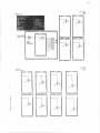
Since the output of the piezoelectric accelerometers is a high impedance charge,
suitable amplifier circuits are required to obtain low impedance output. Charge
amplifiers are the most popular instruments used for this purpose because of their
advantages including high linearity, good frequency response, low influence of the cable
capacitance, and high stability (Kistler, 1995). A typical measurement system that
involves a high impedance piezoelectric accelerometer and a charge amplifier is shown in
Fig. 2.10a (Kistler, 1995).
15
Integrated circuit piezoelectric (ICP) sensors have been developed with an
advanced MOSFET' technology. The ICP transducers consist of high impedance
piezoelectric accelerometers combined with miniature, built-in charge-to-voltage
converter circuits, as shown in Fig. 2.11 (PCB, 1996). As a result, the charges generated
by piezoelectric sensing elements are converted into voltage inside of the transducers
providing low impedance that can be measured by any typical readout instrument
(McConnell, 1995).
Low noise
coaxial cable
II
CI 0 D
Cable
1-
High impedance
accelerometer
Charge amplifier
00
000
Readout instrument
(a) High impedance piezoelectric measurement system
H
I I=
Low impedance
accelerometer
(with miniature
amplifier circuit)
Coaxial cable
Cable
Constant current Power
supply (Coupler)
0
O 00
O 00
Readout instrument
(b) Low impedance piezoelectric measurement system
Fig. 2.10 Comparison diagrams of instrument setup between the high and low
impedance system (Kistler, 1995).
Therefore, the low impedance piezoelectric systems requires only constant current
power supply generated from an external low impedance power supply, or a coupler, to
supply the transducer as shown in Fig. 2.10b (Kistler, 1995).
1 MOSFET is an abbreviation of Metal-Oxide-Semiconductor-Field-Effect Transistor.
16
Built-in Miniature
Amplifier Circuit
Piezoelectric
Sensing Element
Seismic Mass
Connector
Figure 2.11 Cross-section diagram of the ICP accelerometer (PCB, 1996).
The low impedance systems offer potentially lower cost, and more convenient
implementation than the sensors described earlier (Kial and Mahr, 1984; Kistler, 1995).
However, the high impedance sensors used together with charge amplifiers offer
significantly wider range of operation, since the time constant and gains can be controlled
at the charge amplifier. In addition, the high impedance transducers contain no built-in
electronics, therefore, they work in wider temperature range than the low impedance
system (Kistler, 1995).
The overall FRF of a measurement system of the low impedance (ICP)
accelerometer, IMO is (Dally et al., 1993)
I-IL(co)=
where
Vo
sv Ao
1
+ j 24"
j (TC1)
j (TC) co
(co) 1+ j (TC1)- co 1+ j -(TC)
oox
(co)
1
2
- the system's sensitivity (volts/g).
Ao
amplitude of the acceleration applied to the transducer (g),
Vo
- the amplifier output voltage (volts),
0),
- the natural frequency of the accelerometer,
the damping ratio of the accelerometer,
TC1
- the time constant of the power supply,
(2.2)
CO
17
TC
the time constant of the miniature amplifier in the transducer, and
j
the imaginary unit, j =
.
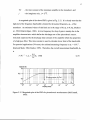
A magnitude plot of the above FRF is given in Fig. 2.12. It is clearly seen that the
high end of the frequency bandwidth is limited by the natural frequency, con
,
of the
transducer. An estimated values of this limit are in the range of 0.1con to 0.3con (Dally et
al., 1993; Briiel & Kjxr, 1982). At low frequency the drop of gain is mainly due to the
amplifier characteristics which define the discharge rate of the piezoelectric sensor.
Concisely expressed by the discharge time constant of the amplifier which has properties
of a high pass filter. This time constant is used to calculate lower limit of the bandwidth.
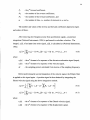
For practical applications (5% error), the minimal measuring frequency is we = 3TC -I.
(Kail and Mahr, 1984; Kistler, 1995). Therefore, the overall measurement bandwidth, f,,,
is
3. TC
<
< 0.3
co
[Hz]
2ir
(2.3)
Magi tide (dEj
50
11
IHLI
0
11
11
11
11
-50
con
-100
1 0 -2
101
10°
101
102
Revery (radIsec)
103
Figure 2.12 Magnitude plot of the FRF of a piezoelectric accelerometer (McConnell,
1995).
18
Application of piezoelectric accelerometers to measure transient vibrations
requires additional consideration. Transient signals may contain DC signal components
that are strongly attenuated as shown in Fig. 2.12. The result can be a drift in the
response signal. The amplifier's time constant must be considered in the error analysis in
such cases. Table 2.1 presents the time constant necessary to limit the error in measuring
various transient signals (Dally et al., 1993).
To visualize motion of the 6-DOF plate considered in Section 2.4, acceleration
signals have to be converted to displacements. Although performing double-integration
on acceleration signals for this purpose seems possible in theory, its implementation is
difficult. Combined distortion of signals measured by piezoelectric accelerometers
usually results in a gradual change of the output voltage (drift). This change is as a
relearn unknown function of time since drift may result, in addition to the distortions
caused by the dynamics of the amplifier, from changes of temperature, line voltage or
amplifier characteristics.
Time Constant Required for Limiting Error
Pulse Shape
2% Error
5% Error
10% Error
50t1
20t1
lOti
25t,
10t,
5t1
A
16t1
6t,
3t1
B
31 t,
12t,
6t,
E'---- ti "U.
___ _TError
Rectangular Pulse
.........--
I- Error
.....iiii 7
Triangular Pulse
1.--
' Ate`,
--..--:.
Half-sine Pulse
..
Error
Table 2.1 Effect of time constant on the error in measuring various transient responses
(Dally et al., 1993).
19
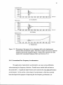
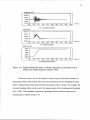
Low frequency measurement errors discussed above are strongly amplified when
integration is applied in the process of converting accelerations into displacements.
These errors are illustrated by the following example involving monitoring displacements
of one point of the plate (see Section 2.4) in response to an impulse force acting on it.
Kistler® model 8702B25M1 piezoelectric accelerometer (Kistler, 1995) is employed to
measure the acceleration of this point. A signal from the accelerometer after subtracting
the DC offset is shown in Fig. 2.13a. It is known that, given enough time after the force
impulse, vibrations die down and the investigated point of the plate returns to its initial
position. Although no drift is noticeable in the acceleration signal, its presence is evident
after its integration, i.e., in the velocity signals which rise gradually as shown in Fig.
2.13b. The displacement signal shown in Fig. 2.13c, which is obtained by applying
another integration, has clearly visible drift, strongly exceeding the level of vibrations
caused by the force impulse.
The primary solution to the drift problem in this research is the use of high-pass
filters to suppress the low frequency components (drift) in the acceleration signals.
Suitable high cut-off frequency has been selected by determining experimentally
characteristics of the transducer. For this purpose, a power spectrum of the acceleration
measured from the stationary (i.e. at rest) sensor was examined. The cut-off frequency
was selected to be above the frequency of the dominating components appearing in the
spectrum. The results obtained by applying high-pass filters (between each integration) to
the signals measured from the excited (vibrating) system are shown as dashed lines in
Fig. 2.13b and 2.13c.
A side effect of using high pass filters are distortion of the signals manifesting
themselves as a phase shift at lower frequencies. These distortions can be clearly visible
in signals having broad frequency contents, such as a squarewaves or impulses. It goes
without saying that high-pass filters are acceptable only for visualizing vibrations of
objects with a frequency higher than the selected cut-off frequency.
20
Acceleration (rn/s2)
10.0E+0
5.0E+0 -
0.0E0
-5.0E+0 - 1 0.0 E+0
0.03
0.01
0.02
0.03
0.04
0.05
0.08
0.00
0.10
time (sec)
0.07
0.013
0.0E/
0.10
time (sec)
0.07
0.08
0.00
0.10
0.00
0.017
0.08
0.08
(a) Acceleration
Velocity (m/s)
8.0E3
4.0E-3 2 .0E-3 -
0.0E+0
-2 .0E-3 -
- 4.0E3
0.00
0.01
0.02
0.0:3
0.04
0.05
(b) Velocity
Displacement (m)
15.0E8
10.0E8 5.0E-8 0.0E+0
-5.0E-8
0.00
0.01
0.02
0.03
0.04
0135
time (sec)
(c) Displacement
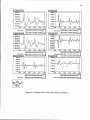
Figure 2.13 Illustration of the impact of a low frequency drift on the displacement
obtained from acceleration signal. Solid lines in figures (b) and (c) represent
integrated and double-integrated signals. Dashed lines represent the same
signals after using digital high-pass filters (see Section 4.3.2).
2.4.2 Conventional Low Frequency Accelerometers
The application of piezoelectric accelerometers can cause serious difficulties
when measuring low frequency vibrations. Possible errors include drift and noise as
discussed above. A significant improvement can be achieved by using high performance
accelerometers. In this section, various types of accelerometers, which have recently
been developed with a purpose of improving the low-frequency performance, are
21
reviewed. These new accelerometers are recommended for application in the
visualization technique presented in this thesis.
Variable capacitance microsensors are designed for a measurement of low
frequency acceleration, inclination, and shock vibration (Endevco, 1996). They employ a
capacitance sensing element that is composed of a very small seismic mass chemically
etched from a single piece of silicon and positioned between two electrode plates. As the
seismic mass deflects under accelerations, the capacitance between these plates changes.
With a signal conditioning circuit, position of the sensing mass is detected and converted
to an output voltage. To prevent excessive shock motion, the sensing mass is damped by
a gas damper resulting in an increase in the measurement bandwidth from DC to 2000
Hz, depending on the sensitivity (Kistler, 1995).
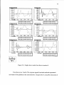
Fig. 2.14a shows example acceleration signal acquired by a capacitive
accelerometer, Kistler® 8302B2S1 (Kistler, 1995) mounted on a rigid object. This object
is slowly moved from one position to another, 7.8 mm away. The initial portion of the
signal (0 - 0.09 sec) representing an output signal of the stationary accelerometer is used
to calculate the value of its DC offset. This value is next subtracted from the signal, and
the resultant is integrated twice to obtain the velocity and displacement measured by the
sensor. These latter signals are shown in Fig. 2.14b. An inspection of the measured and
actual displacement over the period shown in the figure indicates a suitability of the
sensors under consideration for visualization of vibrations with frequencies down to as
low as 2 - 5 cycles per second.
22
Acceleration (m/s2)
time (sec)
(a) Acceleration signals
Velocity (m/s)
.
time (sec)
(b) Velocity signals.
Displacement (m)
8.0E-3
8.0E3
4.0E-3
2.0E-3
0.0E+0
-2.0E3
0.00
0.10
0.20
0.30
0.40
0.50
0.80
0.70
0.43
0.1:0
time (sec)
(c) Displacement signals.
Figure 2.14 Signals obtained by means a variable capacitance accelerometer and its
results from double-integration (Kistler, 1995).
Still better sensors can be developed by improving the measuring technique for
detecting position of the seismic mass since the acceleration can be calculated from the
relative displacement between the seismic mass and the sensor's body. For example, the
electron tunneling effect can be used in the measurement of this displacement (Rockstad
et al., 1992). The transducer consists of a miniature silicon cantilever that acts as a
sensing mass as shown in Fig. 2.15.
23
Suspended proof mass
Apply deflection voltage
Sensor housing
Measured tunnel current
Figure 2.15 Schematic illustration of a single-element electron tunneling accelerometer
(Rockstad et al., 1992).
The cantilever is a gold-coated electrode and supported over the other electrode by
a small spacing that is maintained constant by a feedback circuit applying voltage bias to
the electrodes. When subjected to an acceleration, the cantilever tip deflects, thus,
changes 'tunnel' current between the electrodes. The feedback circuit then controls the
electrostatic voltage such that it returns to its initial position. The variations in voltage
required to maintain constant distance between electrodes indicates the sensor's
acceleration. This voltage is free from hysteresis and drift, and insensitive to temperature.
The FRF cover the range from DC up to 5000 Hz (Rockstad et al., 1992).
Another approach of the low frequency measurement is the use of a piezoresistive
element to detect the motion of the seismic mass. These elements are mounted on a beam
that suspends the micromachined silicon seismic mass as shown in Fig. 2.16. Bending of
the beam caused by the accelerated mass yields a strain that is detected by the
piezoresistor. With a bridge circuit, the changes in resistance are converted to an output
voltage.
24
Figure 2.16 A cross section of the piezoresistive accelerometer (IC Sensors, 1997).
2.4.3 Multi Directional Accelerometer
To describe a rigid body motion in 6 -DOF, at least six linear accelerometers are
required (see Section 2.4). The number of transducers can be minimized by using multiaxis accelerometers, resulting in a reduction of equipment cost. PiezoBEAM® transducer
from Kistler® involves a pair of cantilever beams made of a piezoelectric ceramic material
as shown in Fig. 2.17. The beams are sensing elements that are constructed in a T-shape.
By comparing the phase difference of the electrical charge signals from both beams, the
linear and angular accelerations can be calculated (Kistler, 1996).
Figure 2.17 A cross section of the PiezoBEAM® accelerometer (Da lly et al., 1993).
25
2.5 Closure
Visualization of vibration in theoretical analysis is introduced. The mode shapes
from the theoretical vibration analysis provide graphical representation of coordinates'
relative motion in the system at certain frequencies. The visualization technique is
proposed in which actual movement is detected experimentally using accelerometers. By
studying characteristics of the piezoelectric accelerometer measurement system, problems
in the visualization method are presented as limitation of measurement at low frequency
caused by discharge of output voltage. Higher performance accelerometers are reviewed
and suggested for improvement direction. In the next chapter, concepts of the proposed
visualization technique are described. These concepts include the use of sensors in the
signal based vibration visualization and the use of a mathematical model to improve the
visualization in the model based vibration visualization.
26
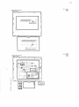
CHAPTER 3
MODEL BASED VISUALIZATION OF VIBRATIONS
The background and essential characteristics of the model based vibration
visualization are presented in this Chapter. Algorithms implemented in this thesis and an
outline of future work are discussed. The model based vibration visualization comprises
two stages. The first stage, a signal based vibration visualization, is developed in this
thesis. The second stage, proposed as the future work, is an improvement of the above
visualization by using the system's mathematical model. An experimental model of
commercial dynamometer is selected as a mechanical system to be visualized. Since a
mathematical model of this dynamometer is employed for generating the estimated
responses to applied excitation signals, a technique used to obtain this latter model is
reviewed at the end of this chapter. The same model is also used to interpret
experimental results in Chapter 5.
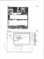
3.1 An Overview and Definition of the Proposed Visualization Technique
The proposed visualization program has been developed to use real signals from
sensors attached to vibrating rigid bodies for generating animated motion of these bodies.
Together with the acquired signals, a mathematical model of the dynamic system
comprising the bodies is also used to detect and suppress errors in the acquired signals.
The entire visualization scheme is implemented in two stages. The first stage,
referred to as 'signal based vibration visualization', is the focal point of this research. A
suitable methodology discussed in detail in chapter 4 facilitates visualization of vibrations
of rigid bodies by using signals from acceleration sensors attached at precisely defined
locations of these bodies. Set of data collected from these sensors are referred to as
27
`signal based responses' (SBR). Typically, conducting one experiment generates one
SBR.
In the second stage of the visualization each specific SBR is analyzed to detect
possible errors in recorded signals by using a mathematical model of the system under
consideration. This is accomplished by comparing the SBR with a hypothetical response
which is generated by stimulating the model with the actual input signals that acted on the
physical system. These generated hypothetical output signals are referred to as 'model
based responses '(MBR). In addition to detecting errors (e.g. drift) in signals from the
actual sensors the knowledge of mathematical model facilitates significant suppression of
these. Thus, the obtained enhanced visualization is referred to as the 'model based
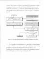
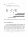
vibration visualization'. Fig. 3.1 shows in the form of a flowchart the essential units of
the developed visualization and software.
Stage 1
Vibrations in
Mechanical
System
Measured
Signals
Signal Based
0 Vibration Visualization
Mathematical Model
of the System
Signal Based
Response
T
....11101
Model Based
Response
Comparison
and
Correction
.0
Model Based Vibration Visualization
Figure 3.1 Flowchart of model based visualization of vibrations.
Corrected
Display of
Vibrations
Stage 2
28
3.2 Signal Based Vibration Visualization
A flowchart of the methodology used in the signal based vibration visualization is
illustrated in Fig. 3.2. Vibrations of a mechanical system are detected by means of
accelerometers attached to the system. The acceleration signals acquired using a data
acquisition (DAQ) system are processed in two steps to obtain generalized coordinates2.
These steps are designated in the figure as the Signal Processing and Generalized
Coordinate Calculation. Finally, the processed data are transformed into three
dimensional (3-D) animated pictures representing the vibrations of the mechanical
system.
Vibrations
Mechanical
System
Accelerometers
cceeromeers
Data
Acquisition
System
Signal
Processing
Generalized
Coordinate
Calculation
3-D
Animation
Figure 3.2 A flowchart representation of the methodology developed for the signal based
vibration visualization.
The major purpose of the signal processing stage is the calculation of variables
necessary for describing spatial motion of the system from measured data. This is
accomplished by double integration of the acceleration signals to obtain translational and
rotational displacement variables required for the visualization. An implementation of
the integration is difficult since various errors distort the measured signals, as discussed
in Section 2.4.1. As a result, the animated vibration of the system may be quite different
from the actual ones. A software package developed in this thesis comprises all functions
represented in Fig. 3.2. It also suppress a large portion of errors in the measured signals
by using rudimentary techniques, namely subtraction of the average value of the signal
and high-pass filtering. These techniques are well documented in the professional
2 Definitions of the generalized coordinates is introduced in Section 3.5.
29
literature and applied in commercial systems (see Section 2.3). To achieve further
attenuation of errors it is recommended to use a constitutive mathematical model of the
system whose vibrations are visualized. A full implementation of this new approach is a
complex task, beyond the scope of this thesis. The remaining part of this chapter contains
a discussion of the ideas involved in implementing constitutive mathematical models for
the purpose of error suppression.
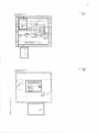
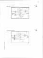
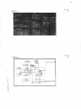
3.3 Model Based Vibration Visualization
The model based vibration visualization is based on an assumption that vibrations
of a system can be estimated if its mathematical model is known. To model the system, a
priori knowledge of the system is required.
There are various classifications of dynamic systems depending upon the features
of these systems that are interest. A classification proposed by Chung (1991) is
applicable in this research. It divides dynamic systems based on their features relevant to
parameter identification as shown in Fig. 3.3. Shadowed boxes indicate the path
applicable in this research
.
Stochastic
Dynamic
systems
SISO
Time-invariant
MIMO
Nonlinear
SISO
Time varying
MIMO
Deterministic
Time-invariant
Linear
SISO = Single-Input-Single-Output
MIMO = Multi-Input-Multi-Output
I 4=ol
Time varying
SISO
MIMO
Figure 3.3 Classification of dynamic systems (Chung ,1991).
30
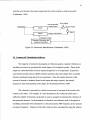
A system that has several input signals that stimulate responses on several outputs
as shown diagrammatically in Fig. 3.4, is termed The multi-input multi-output (MIMO)
system.
Input -
(u(t))
System
Gs
Output
(Y(0)
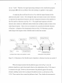
Figure 3.4 The MIMO system.
Dynamic mechanical systems under consideration are MDOF systems and also
MIMO systems which can be described by the following vector-metric equation. (Chung,
1993)
Y(s) = Gs(s)U(s)
(3.1)
where
Y(s) Laplace transform of the output vector y(t), i.e., a vector whose elements
are all output signals,
U(s) Laplace transform of the input vector u(t), and
G,(s) the transfer function matrix of the system.
The matrix GS(s) has nxm elements, G, (s), where i = 1,2 ..., n and j = 1,2 ..., m.
Each of these elements is a rational polynomial representing a transfer function between
input ith and output ith for a system with m inputs and n outputs.
It is usually difficult to estimate the exact transfer function, Gs(s) of an actual
physical system. Therefore, an Equivalent System is often introduced, which retains the
major properties of the original system but at the same time has a transfer function model
that can be experimentally estimated. If this latter transfer function, GE(s), is obtained by
31
means of a modeling technique, the estimated response, yE(t), can be calculated from the
input, u(t), acting on the original physical system and the transfer function of the
equivalent system, GE, using the following relationship
yE(t) =
GE(s)U(s) J
(3.2)
where
L' denotes the inverse Laplace transform operator.
Since the model based vibration visualization employs the estimated response, yE,
to compare with the signal based response (see Section 3.2), the accuracy of yE is of
utmost importance. Thus, high accuracy of the system's modeling and estimation are
necessary. This can be achieved by applying accurate system identification techniques
introduced in Section 2.2. A structure of the model, i.e., form of equations, is derived
such that it captures the essential physical laws governing the system's behavior.
Parameters in this model structure are estimated from the input and the output signals.
The estimation procedure can be performed in real time, which means that the
identification takes place at the same time as the system's vibrations are measured.
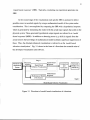
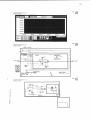
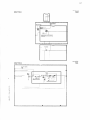
The model based vibration visualization is an extension of the signal based
vibration visualization presented in Section 3.2, in which the system identification and
model response analysis technique are included. A flow diagram of the enhanced
visualization is shown in Fig. 3.5. The visualization begins with the measurement of
vibrations of a mechanical system by means of sensors (accelerometers) which is
performed by the Data Acquisition (DAQ) system. The measured signals are processed
in the Signal Processing unit, and the Generalized Coordinate Calculation unit yielding
the 'signal based' response. In a parallel thread, a suitable mathematical model of the
system is derived analytically in the Model Derivation unit. The modeling technique that
involves symbolic computations can be applied to generate a structure of the model,
while the essential unknown parameters are represented as symbolic coefficients in
model's equations (Rehsteiner et al., 1997). To complete the model, a system
identification is applied to estimate the unknown parameters. As already explained in
32
Section 2.2, this technique employs an iterative procedure that adjusts values of the
model's parameters in order to minimize a difference between the signals recorded from
the sensors and calculated responses of the model.
I Input
4
Information About the System
Mechanical
System
4
Vibrations
Model
Derivation
DAQ System
Measured Input
Model Structure
Measured Output
System Identification
Estimated Parameters
Feedback Command
4
Estimated Model
Model Based Response
.4
Response (Generalized Coordinates)
Generator
YE(t)
4
Interactive
User
Interface
Comparison and
Correction
Signal Processing
and Generalized
Coordinate
Calculation
Signal Based Response
(Generalized Coordinates)
See Section 3.2
Corrected Response
Display of
Vibrations
Figure 3.5 Block diagram of the model based vibration visualization.
The complete analytical model is represented by the analytical generated structure
and the estimated parameters. This model is employed for generating the model based
33
response using the stimulation acting on the actual tested system3. Information from the
estimated model is also used in the Comparison and Correction unit to generate suitable
feedback commands for tuning of the Signal Processing unit and the Response Generator.
The comparison and correction unit is also responsible for generating messages and
warning to the user.
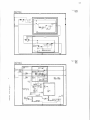
A flowchart of the Comparison and Correction unit is shown in Fig. 3.6. This
unit comprises Data Analysis and Filter Tuning sub-unit in which the actual and
estimated responses of the system are compared. The comparison can be based upon
various indicators, such as, the coherence function (Bendit and Piersol, 1980). Results
from the comparison are used for the validation of the acquired data and diagnosis of
likely errors.
Comparison and Correction
Signal Based Response (SBR)
Corrective Filters
Corrected
Response
Display of
Vibrations
jControl
and
Results
Model Based Response (MBR)
Data Analysis and
Filter Tuning
Estimated Model
(Structure and Parameters)
Interactive
User
Interface
Information about the System
4
Feedback Command
To Signal Processing unit and Response Generator
Figure 3.6 Block diagram of the Comparison and Correction unit.
3 For example, a force impulse from an impact hammer.
34
For example, if the coherence results show discrepancy between both responses
above a certain pre-set level, the control unit informs the user about the incompatibility of
the data via the Interactive User Interface. The user may insist to display the response by
sending a command to the Data Analysis and Filter Tuning unit. Relevant correction
methods may be employed, for example, subtracting mean values of the estimated errors
from the signal based responses or re-processing the signals using new parameters set in
the Feedback Command.
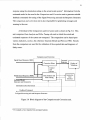
An alternative method for the visualization improvement is to compare directly
the acceleration signals acquired from the sensors with acceleration responses calculated
from the model. A block diagram corresponding to this better method is shown in Fig.
3.7. The drift embedded in the signals can be detected and eliminated by comparing
quesi-static values of acceleration signals obtained by these two essentially different
approaches. One significant advantage of this method is the elimination of high-pass
filters (see Section 4.3.2) which, as an effect, introduce distortion into the signals
recorded from the sensors.
The above discussion of the algorithms facilitating enhanced visualization of
vibrations in mechanical systems addressed only the main aspects of this complex
problem. There are numerous ways to implement these algorithms and broad spectrum of
additional signal processing methods that can be applicable. More research is needed to
find the most reliable and efficient methods.
35
Input
Information About the System
-4
V
Model
Derivation
Mechanical
System
4 Vibrations
DAQ System
V
Measured Output
Model Structure
System Identification
Estimated Parameters
Estimated Model
V
V
I
Model Based Response
(Accelerationa)
Response
Generator
Comparison and
Correction
Interactive
User
Interface
Signal Based Response
(Accelerations)
Feedback
Command
Corrected Response 4
Signal Processing and
Generalized Coordinate
Calculation
4
Display of
Vibrations
Figure 3.7 An alternative flowchart of the model based vibration visualization.
3.4 Feasibility Study of the Visualization Enhancement
An application of the mathematical model is investigated to generate responses of
a mechanical system stimulated by known input signals. This system is a physical model
of a high performance dynamometer (Kistler® type 9257A; Kistler, 1995). The
dynamometer is a multi-component force sensor comprising the major parts shown in Fig.
3.8. A platform is supported by four piezoelectric-based sensing elements. When a force
is applied to the workpiece attached to the platform, the platform is moved from its
equilibrium position, thus causing the piezoelectric sensing elements to deform. Electric
36
charges generated from the deformations are measured and combined to calculate the
applied force. If the platform is considered as a rigid body, its motion is described by six
degrees of freedom: three translations and three rotations as previously described in
Section 2.4.
Figure 3.8 Major components of the dynamometer (Kistler, 1995).
The signal based vibration visualization technique proposed in this Chapter is
applied4 to visualize vibrations of the dynamometer's platform. A linear model of the
dynamometer (Chung 1993 and Chen 1996) is used for calculating theoretical vibration
responses. Calculated and measured generalized coordinates are then compared. Results
and errors of the visualization are analyzed. The main research subjects dealt with in this
thesis and pertain to model based visualization are schematically shown in Fig. 3.9.
These subjects are laid out in the figure such that they resemble the flow chart of signal
based visualization algorithm shown in Fig. 3.2.
4 Detailed discussion of the experiments is presented in Chapter 5.
37
Force
transducer
Measured input forces
and moments
Modeling of
Dynamometer
(Section 3.5)
Information about
process and sensor
ynamo-
Accelerometers DAQ system
(Section 4.2)
Excitation
(Input
force)
II
L.
Model based response
(generalized coordinate)
Comparison
(Section 5.4)
3-D Animation
Signal Processing
of
(Section 4.3) and
Vibrations
Generalized
ill1=1M11011 (Section 4.6)
Coordinate
Measured
Calculation
Signal based response
output
(Section 4.5)
(generalized coordinate)
Mechanical System
under Consideration
Figure 3.9 Main research subjects pertaining to model based visualization.
3.5 Modeling of the Dynamometer
Practical application of the model based visualization hinges upon the capability
to derive analytical models of the systems under consideration efficiently and rapidly. A
modeling technique of the dynamometer proposed by Chung (1993) has been used in this
thesis. This technique using Lagrange's equation has been combined with computeraided symbolic computation proposed by Chen (1996). The modeling involves the
following four stages: (1) decomposition level in which the physical system is converted
into components where motion attributes are assigned to each part, (2) mapping and
identification level where the energy attributes are assigned to each decomposed
component, (3) synthesis level in which generalized coordinates are assigned to the
components and the mathematical model is built, and (4) modification level where the
generated model is checked the analytical model specifications or experiment results
(Chen, 1996).
38
This modeling methodology is applied for modeling the dynamometer under
consideration installed on a machine tool (Fig. 3.10). The machine tool is treated as a
linear, rigid-body system and it is decomposed into four major units shown in Fig. 3.11.
Spring-dashpot elements represent bolts, joints, and guideways the link all components
(Chen, 1996).
Traveling column
Tool storage
liii
Spindle carrier
Tools
(cutters)
Tool
interchange
arm
Spindle
.4,1%t
..
001.
Dynamometer
irre4101
-41141.
Bed
Saddle
Figure 3.10 A high speed machine tool (Kalpakjian, 1992).
Column of the
Machine
Spindle Assembly and Tool
Workpiece attached to the dynamometer
Dynamometer's Platform
Four Sensing Elements
Part of the
System dealt
with in Sections
3.5.1-3.5.3
Machine Table and Dynamometer's Base
Floor
Figure 3.11 A simplified model of the machine tool from Fig. 3.10 with the
dynamometer installed (Chen,1996).
39
3.5.1 Mechanistic Model
The dynamometer described in the preceding section, whose simplified
mechanical diagram is shown in Fig. 3.12, is considered as a MIMO system with an input
vector, u(t), and output vector, dG. The input vector has in a general case twelve
components (Chung, 1993)
u(t) = [ F(t) M(t) DT(t) RT(t) ]T
(3.3)
where
F(t) = [ F., Fy Fe ], forces acting on the platform,
M(t) = [ Mx My M, ], torques applied on the platform around XG, YG and 4 5,
respectively,
DT(t) = [ XT YT ZT], translational motions of the dynamometer's base, and
RT(t) = [ OT OT VT ], rotational motions of the dynamometer's base.
The output vector, dG, is a set of variables describing position and orientation of
the rigid platform. This set is called a generalized coordinate list, dG, that is defined as
follows
dG =[ x y z 0 0 tif ]r
(3.4)
where
the x, y, z, 0, 0, tit are defined in Section 2.4.
Under simplifying assumption that the dynamometer's base is fixed and DT and
RT are equal to zero, the input vector in Eq. 3.3 reduces to a 6x1 vector
u(t) = [ F(t)
M(011.
5 Definitions of axes are introduced in Section 2.4.
(3.5)
40
External Force, F
Xx
Y
Figure 3.12 Simplified mechanical model of the dynamometer under consideration
(Chung, 1993).
When the workpiece is being machined, an external force, F(t), is acting on the
platform as shown in Fig. 3.12. The acting point of the force is located at axa + ayja +
azG , where iG, jG and kG are unit vectors of the XG, YG and ZG , respectively. The
quantities ax, ay and az are signed numbers measured from point G along the XG, YG and
ZG directions. The external force contains three components, Fx , Fy and F, which also
generate three associated moments (A 1xF, MyF, MZF) with respect to the center of gravity
MxF = ay.F, azFy
(3.6)
MyF = -ax.Fz + azFx
(3.7)
My = a,y ayF,
(3.8)
The three components of the measured force and three resultant moments acting
on the platform represent a complete set of independent variables in the equations of
motion. This set is henceforth referred to as a forcing function vector, Fe. It is obtained
41
by combining six elements of the simplified input vector u given by Eq. 3.5 with the
moments My, MyF, My,
Fe = [ Fx Fy
Fz (mxF+ MX) (myF + my) (lzF+Alz)11.
(3.9)
F, , Fy and Fz, are signed numbers that are positive if they are in the positive
directions of the respective XG, YG and ZG axes. The above equation can be rewritten in
terms of the input vector u and a matrix C (ax, ay , az) whose exact form is given in
Appendix B.
(3.10)
Fe = C u-u
By applying Lagrange's method, the equation of motion can be derived in a
matrix-vector form (Chung, 1993)
m aG + c aG ± k dc = Fe
(3.11)
where matrices m, c and k are listed in Appendix B.
3.5.2 State Space Model
Since the dynamometer is a MIMO system, its analysis can be greatly simplified
by introducing the state space model (Franklin et al., 1994). One of the main reason of
using the state space model in this research is the availability of commercial software
packages, such as Matlab® or Mathematica®, that allow easy implementation of
complicated algorithms developed in control theory for the investigation of MIMO
system.
To transform the equation of motion into the state space form, Eq. 3.11 is first
rearranged as follows
do
. m -'k do
m-lc do + m-1. Fe
(3.12)
42
Next, by introducing an auxiliary vector dGD such that dGD = dG , can be written
as (Peters and Mergeay, 1976)
iii = Aq+B-u
(3.13)
dG = Cq + Du
(3.14)
where
the vector containing 6 generalized coordinates,
dG
q
- the vector of state variables defined as
q = [dG
(3.15)
dcDiT
The dynamic matrix A and control matrix B contain elements of the matrices m, c
and k from the equation of motion model, Eq. 3.11. Their form is
A=
06 x 6
mc
-M-1 k
x
(3.16a)
-1
Cu
B = m-1
where I
16 x 6
is a 6x6 identity matrix and O
(3.16b)
is a 6x6 zero matrix.
The observation matrix C and the direct transmission matrix D represent
relationships between dG and q, as well as, dG and u, respectively. If the output of the
state space equation is desired to be the generalized coordinates vector, dG, the form of
matrix C is given by Eq. 3.16c. Since no direct relationship exists between the
generalized coordinates and the input vector u, the matrix D is a zero matrix.
C=[I
D=0
0
)T
(3.16c)
(3.16d)
43
3.5.3 Transfer Function Model
The state space model can be transformed into the transfer function model by
taking Laplace transformation of Eq. 3.13 and 3.14. Under the assumption of the linearity
and time-invariance, the matrices A, B, C, and D are considered as constant matrices.
For zero initial conditions a new set of equations is obtained
sQ(s) = AQ(s) + BU(s)
(3.17a)
DG(s) = CQ(s)
(3.17b)
where
Q(s) is the Laplace transform of the state vector, q(t),
DG(s) is the Laplace transform of the generalized coordinates vector, dG(t).
By applying rules of linear algebra, the above equations can be converted into the
following input-output form.
GE(s) = DG(s)/U(s) = C.(s.112),12
(3.18)
The above equation encapsulates the relationship between the input vector
(external forces and moments) and the output vector (generalized coordinates) in the
transfer function matrix GE. There are several methods to generate responses to actual
input signals by using the transfer function model of the dynamometer. One approach
that is conceptually simple involves the following equation
dm(t) = L-1[ GE(s)-Um(s)
(3.19)
where
U(s)
Laplace transform of the actual input signal u(t),
dm(t)
generated model based response,
- inverse Laplace transform operator.
Commercial software packages such as Mat lab® or Mathematica® allow quick and
easy calculation of these responses.
44
The state space model of the dynamometer presented above is used in Section 5.4
to generate the response vector dm. The input um is obtained using an actual force signal
from an impact hammer in the experiment. The calculated and recorded responses are
compared and their differences are discussed. A Mat lab® program used to generate
response of the dynamometer's model to the actual excitation is listed in Appendix C.
3.6 Closure
The model based vibration visualization proposed in this research is performed in
two stages. The first stage is the signal based visualization in which vibrations of a
mechanical system are measured and recorded by means of accelerometers and presented
in 3-D graphical animation. In the second stage, the mathematical model of the
visualized system is used to detect errors that can occur in the first stage. A MIMO
model of the actual system is applied to generate estimated responses to the actual
excitation signals. The system identification technique is used to assure high fidelity of
the model.
A dynamometer is used as an example dynamic system. Its model developed in
previous researches (Chung, 1993; Chen, 1996) is employed. This model obtained by
means of Lagrange's method treats the actual dynamometer as a linear time invariant,
MIMO system. Details of a methodology developed for the signal based vibration
visualization applied to a rigid plate are explained in the next chapter. The application of
this methodology and its experimental evaluation are presented in Chapter 5.
45
CHAPTER 4
THE SIGNAL BASED VIBRATION VISUALIZATION
The underlying theory and algorithms employed in the signal based vibration
visualization are presented in this chapter. Convenient coordinate systems and several
crucial procedures are discussed in detail. The entire visualization process is partitioned
into four major steps, namely: 1) data acquisition procedure, 2) signal processing, 3)
generalized coordinate calculation, and 4) 3-D animation procedure.
4.1 Visualization of Machine Vibrations
The visualization of machine vibrations presented below assumes that each
specific part of the machine is a rigid plate with six degrees of freedom (6 -DOF) motion.
This means that six variables, three for translation and three for rotation, are required to
describe three dimensional (3-D) motion of the plate. These variables are formed into the
generalized coordinate list, dG, in Eq. 4.1. Graphical representation of this list is shown
in Fig. 4.1.
dG=[xyz 00 VW
(4.1)
One generalized coordinate list represents one specific location of the plate in
space and is used to generate one picture of the plate in the 3-D space. Hence, a time
series of coordinate lists is needed to create a sequence of pictures that represent motion
of the vibrating plate. A technique to calculate the generalized coordinate lists from
experimental data is discussed below. A method employed to present the results as 3-D
graphical animation is also described.
46
z
4
Figure 4.1 Components of the generalized coordinate list, dG, describing the 'rigid-body'
motion of a plate.
4.1.1 Overview of the Methodology
A flowchart of the algorithm used in the visualization is shown in Fig. 4.2. First, a
simplified mechanical model is developed by dividing the machine into a suitable number
of rigid solids, (e.g., plates). For example, a simplified machine shown in Fig. 3.11
comprises four prismatic solids representing the column, spindle assembly, table, and the
dynamometer's platform with workpiece. Multiple sensors are installed on the machine to
measure vibrations of each prismatic solid.
The solution employed in this research requires nine accelerometers per each solid
to measure its list of generalized coordinates (Padgaonkar, 1975). Acceleration signals
from these transducers are recorded by a data acquisition (DAQ) system which is
controlled by a LabVIEW®-based Data Acquisition Controller program (see Fig. 4.4a).
In the second step the voltage signals from accelerometers are: (1) amplified, (2)
low-pass filtered (anti-aliasing), and (3) converted to acceleration using respective
transducer's sensitivities. Average quasi-static offset voltage having its source in thermal
drift in each sensor is eliminated by subtracting the average (or moving average) value
calculated for each signal. Adjusted signals are numerically integrated twice to obtain
displacement signals. Since signals from piezoelectric accelerometers are affected by
47
drift and noise, direct integration of these signals yields strongly distorted results.
Therefore, digital high-pass filters are employed to remove quasi-static errors.
Angular components of the generalized coordinate list, dG, are then calculated
from the processed displacement signals using equations proposed by Padgaonkar et al.
(1975), as further explained in Section 4.5. Finally, a sequence of generalized coordinate
lists representing consecutive 'snap-shots' is generated for the animation of motion.
The animation procedure uses the homogeneous coordinate transformation
(Wolovich, 1987) to draw 3-D wireframe pictures that present the consecutive positions
of visualized solid. Rapid displaying of pictures generated from each data point (6
coordinates) creates the effect of animated motion. Detailed discussion of animation is
presented in Section 4.6.
Physical
System
Idealization
and
Decomposition
Transducers I
Signals
Selection of
Transducers
Data Acquisition
(LabVIEW® DAQ Controller)
Section 4.2
Signal Processing
subtracting moving average
conversion to physical units
digital high-pass filtering
Section 4.3
1
Simplified
`Rigid Body'
Model
Structure of the
Idealized System
Generalized Coordinate Calculation
application of formulae given by
Eq. 4.10
Section 4.5
3-D Animation
Section 4.6
Figure 4.2 flowchart of the methodology used for the visualization of machine
vibrations.
48
4.1.2 Introduction to LabVIEW® Programming Environment
LabVIEW® is a program development application that uses graphical
programming language, G, to create programs in a flow-chart-like form, called a block
diagram (National Instrument, 1994). Unlike other programming languages such as C,
FORTRAN or BASIC, LabVIEW® relies on graphic symbols rather than textual
statements to describe programming actions (National Instruments, 1994). These
symbols (icons) such as, switches, knobs, and displays represent and resemble elements
found in physical instruments. Because of its appearance, the LabVIEW® programs are
called virtual instruments (VI).
LabVIEW® offers extensive libraries of functions and subroutines, for example,
application-specific libraries for data acquisition, data analysis, data presentation, and
data storage. In data acquisition aspect, LabVIEW® can command DAQ boards to read
analog input signals (with A/D conversion), generate analog output signals (D/A
conversion), read voltage data for processing or other manipulation, and write digital
signals into storage devices (National Instruments, 1994).
A typical virtual instrument (VI) consists of two parts, afront panel and a block
diagram, displayed in two separate windows. In the panel window a user interfaces with
the VI via Controls and Indicators. The Controls simulate instrument input devices and
supply data to the block diagram of the VI. The Indicators simulate instrument output
devices that display data acquired or generated by the block diagram of the VI. In the
block diagram window the user constructs a graphical source code of the VI by wiring
together objects (represented by icons) that send or receive data, perform specific
functions, and control the flow of execution. Fig. 4.3 shows an example of the VI
(variable amplitude sinewave generator) which displays a knob and graph in the front
panel (a) while the calculations take place in the block diagram (b).
49
All visualization programs in this research were written in LabVIEW ®. The
developed set of programs consists of the following major VIs:
1. "Data Acquisition Controller.VI". This program facilitates acquisition of up to 16
vibration signals from transducers attached to a machine. It is further discussed in
Section 4.2.
2. "Signal Processor.VI". This program performs the signal conversion, subtraction of
the moving average, filtering, and numerical integration on the acquired data.
Calculations used in this VI are further discussed in Section 4.3.
3. "Generalized Coordinate Calculator.VI". This program calculates a sequence of the
generalized coordinate lists, dG(t), introduced in Section 4.1. Each list is calculated
from nine linear acceleration signals recorded at any given time instant for each
prismatic solid representing an element of the simplified machine. Equations
employed in the calculations are further explained in Section 4.5.
4. "3-D Animation Generator.VI". This program generates 3-D pictures using a time
series of coordinate lists dG(k),
m is the number of data. The animation is
achieved by rapid display of these pictures.
The above programs can perform their functions individually. Alternatively, each
of them can work as a subprogram that can be run and interfaced from other programs.
Figure 4.4 shows the front panels these VIs. Program descriptions and usage are
explained in Chapter 5 and in Appendix D.
Numeric Control]
4.0
6.0
o fa ao
0.0
Output Graphl..
\\
3,07
:..,.-
7/
io o
.I.1 10
1
\
[DBL]
\
Output Graph]
1[>-, [Du]
N_
1, -,
o
Numeric Contrail
4':
:':
i
120
Sine Wave.vi
(a) front panel
(b) block diagram
Figure 4.3 An example program (virtual instrument) in LabVIEW®.
50
Edit
File
Operate Controls Windows Text Help
21111 In MOM
Number of channel
g
1 (chO)
3
11
unoual
256
Entry number of data
Number of data
II
4
Lir
10000.0
adga or slobs
time mil
Type of DOG
1
111--.4
(re
setting'
Setting
trigger Chi trigger level'
I
PH° III °-°c°
I
1
Real time (sec) MEM Real freq (scans/sec I 10000.00111
-222
-2.83
Continuous mode
ICCOD
Pretrigger data number MEE I =Z. i 1[130 1
R.I4EIE
14
Scan rate (datapoict /sec)
107.0
X axis in dT
1ff
=0:1
limit
,
setting
1__
.2.84
5
Oa
-a-
\
.2.85
4
.2.83
o.00
i
0.01
F
Now di,,plaving the acquired data
1,...S RI
"Save to tie" for Data saving
"Show graph. for [ipplay data
11=111 code
DAC l program
,,,,,, 2.6,
10803 .. ource
am
__
datory
r.P1 Om
a
el
Fix print no.
[Show graph]
Acquire again
1.7
in
save option
no time@ last column
Ompo. Suit, u.).,.*,
0
c_nd.,,,,r,17,
save to tie
I Group Coring
Contra/ & Afeebatrantes Lab
kighor I. ritrogui
xformat a
10.000
cc
Re-acquoing
Stop program
(a) Data Acquisition Controller.VI
Vile
Lout
Er
Controls Windows Text help
Operate
Mb ME MEE
:::iprxtr-roceiror Program
Control Blochotronics Lab
Filler type
P5,1 5 .0. P,....,H. 01,70u Tut, 1_199r
...ow 7Terea Jibra,70
10000 001
liplow
STOP PROGRAM
i
total data
changed Displayed
I 147811
147811 Column
total controls changed
1
I
high cutoff freq: fh L
Feb 97
CHANGE FILTER CONTROL
131
20000.011
131
7
(accelerometer
of let mde
8
,,
x axis 81
2 0E+0
I 10 00
sensitivity
(mV/ unit)
V1
41
1
Z.= MEN
01E3
high limit (volts) low knit
no
Attach signal limits
10 Systeminto
11116)
LI
En
U
es asaani
lime
n°
Wiil° les
tie
Berl Integrate filter 2 Inteigate
1 THOMAS \ T NANA T T MP \ DA T AOFC20-8C.CT R
=I] graph 1 mode Illnput signal
Ye
Deale new
serial number DAQ gain
1100867.00
0
passband lippleldB) Il 0101'
off e' length
stopband
100
attenuationic10) 1 'En
Pala Rename] %PATH:HAS lTHANAT T MP \ DATA 1 CENT -ZA.DAT
Isystemonto rdenarnd
I
10CatIon
!Corner 0 in Z direction
cutoff hew fl ta 0E.01 subtract
filter order
rom fit
sensor type
igh pass
sampling beg [
SP
fiket 3
CU Ma
inverse I
ON
1.0E40 0E4
1
.1.0E +0
2.0E 0
0 00
0.01
0.02
0 03
graph 2 graph 2 mode Putout signal
0 04
0.05
x aids 1$20
0.06
0.07
0.08
point 'save begin 01058
0 09
0 10
0.1
Illsave end 01585
30E-6
2.0E -6
1.06 -6-
-------------
0.0E .0
-2.0E -6-
-10E-60
200
60
600
950
1000
1200
1400
1
630
lobo
2000
220
(b) Signal Processing (double integral) ii.vi
Figure 4.4 Front panels of LabVIEW® programs developed for the vibration
visualization.
51
file Edit Dp e r at e Controls
41 11111111111111
Windows Iext Help
19I1) WHOM...SWIM/1AT THPWATAlASEllrlA.VIZ
rat
Naiemnio *navel
1
1:1..THE114AS TRANAT THPWATA%3F1:211-13C.CTFI
ChannejIn 211gqj
tiel
Y.
tSedenille
In Dreams n Y ciecnon
1169.92600E4
I
Cone. n 2 bad., @channel'
to/nte le Mei
if YES
Canal n X daecticn @channalF1
'Ca nal n Z beaten @ darnel
Wl
fl
3"= x'+1
Ic Datarce n
incesoos4
icaner2 n Y erection @ ehenre4H
Cernet2 ni 2 d...ian @ channel
6ece,ln
P-6-1
torna13 n X *caw @carnalR
Em
Ell ma=
he Dwane. n X erection Immil
Comet] n X beano @charnel
Comer0 n Y dream @channel
iCairm3 n Y &meal @charnel
Oat. mai
Gene. armed aonscr...1e moo.
Fal Emu. JaMMEMEMEAEMMEAEMME samiaumEmmi
om EmmiEMEME30111FAEOWAEMMEAmCaammEaml
LaamMEAmEmmiEsamMEJamMEAcomaamEmol
Ea am) 3x16 snic] amea Etam sem
EmEMEAmMEAmMEAmME.acumME3MMEAPIMME2EMM
19E1
UM:A DOE =I IICI3
LEA SIII:11 l 112121E £111E1 EOM
Rum 2ExE,
,.1 EMU WWI ET9P4
311:1E £11E111 MO MINI 01=1:1 MEM
SEEMS IDEA PA .1P+7 Min MAU SEM
AmEgammEmmiEmmaammEaaWammElamm
AMMEMEME3EMMEAEMMEMEWJEWJEMME3ami
WED EURG 11=F1 MEE MEI EEXII
LIEMMUUMMEmmilEsamMIDIMIE301.3m. MEM
(c) Generalized Coordinate Calculator.VI
File
erate
edit
111%
NM 5- 4,a-20_ 4at
males T. Yiepsitplx.i. Mech. Eno. Dept.
.74,7,-.:", aa 1.1ru,riav
to,..5... 2-
&splayed* Panslation
total data
I iID
103
WA lee
I3D graph
10e
rotation magnify
Date filename
10-
ri
=1, 8 yes
display a
aLt4At g=jfil
step
delay
Parses
Control a Neel mammies Lap
Text Hop
Windows
controls
<
F ono fee
Rol shift
(would el
360.0200.0-
PiPsh shift
[around YI
36ao200.0-
Yaw shift
(amend zl
360.0 -°
2(1110-
0.0-
0.00.0180-0- -cs -180.0- ,...180 0
Viii J
5L
\THOMAS % THANAT.THMATNCENTZA.COD
750E450.0E40
-
111111111PAO
25.0E40-
-
._41°.7.2111411111111111A,
0.0E4-
e
.74.41.404Pr
r_m p
-25.0E4-
i5a75.:::
-
data
100.0E40
1P
.10 0.0 E. 0
-
4
-
4
12 5. 0 E. 0
15 0.0 E. 0 -
175.0 E ..0-2 0 0.0 E 4
-225.0E+0
oi:i.i) iimii.o 20011E4 300.0E.0 400.a
400.CE.0 -300.0Ee0 -200.'0E41 -ioa0t4
Meal vaph
E-9
martinets
Ssatermirio fiarsarne %ID,
11.2±1
ILt115fil
2.1E -90.0E+0
-2.0E-9
-40E 9
accE4
20.00E-3
Horizontal dap* FI
Vertical dtsplay
peed (sec)
..aEll=
Platform @cokann index]
1E]
40.00E-3
ELM
60.00E-3
1-3813.90
80.00E-3
lip
100.00E-3 120.00
A
%darn
Base
Refatence
option to sensor frame
X axes
Wear.d for dynamo-cornor inference
Y axis
!Erase @ column mdcerl
Z axis
(d) 3-D Animation Generator.VI
Figure 4.4 (continued) Front panels of LabVIEW® programs developed for the vibration
visualization.
52
4.2 Data Acquisition System Used in Vibration Visualization
A standard data acquisition (DAQ) system comprises the following basic
components: (1) a controller, (2) a signal conditioner, (3) a multiplexer and amplifier,
(4) an analog-to-digital converter (ADC), (5) a storage unit or a memory unit, and
(6) a readout device (Da lly et al.,1993). The DAQ system employed in this research is a
computer-based instrument. The control part is implemented in LabVIEW® program.
The memory part and the readout device are added as a desktop computer. The ADC,
multiplexer and amplifier are provided in a plug-in DAQ printed circuit board type AT-
MI016E2 from National Instruments (1994). Low-pass filters serve as signal
conditioners to prevent signal aliasing. A schematic diagram of the employed DAQ
system is shown in Fig. 4.5. Further details are given in Section 5.1.
Physical Model of a
Dynamic System
Signal Couplers and Amplifiers
Impact Force and
Accelerometers
Kistler® 8702B25M1
(Kistler, 1996)
Kistler® 5128A
PIEZOTRON coupler
(Kistler, 1996)
Anti-aliasing Filters
Precision 88B (Precision, 1989)
and
Datel® FLJ-D6LA2 (Datel, 1987)
ADC, Multiplexers, Amplifiers
National Instrument® AT-MID-16E2
(National Instruments, 1995)
LabVIEW® DAQ program
"Data Acquisition (version 2.6 s).vi"
Figure 4.5 A block diagram of the basic data acquisition system used in this research.
53
4.2.1 Anti-aliasing Filtering
The `aliasing' phenomenon can occur when converting an analog signal to a
digital data with sampling frequency lower than the minimum required rate. To prevent
this phenomenon, a minimum sampling rate should be set at least twice of the highest
frequency component of the measured signal, or the Nyquist frequency (f*). Practically,
the sampling frequency (fs) is set to be 2.56f (Doebelin, 1990).
Anti-aliasing filters are employed to assure the aliasing prevention regardless the
actual spectral contents of recorded signals. They are analog low-pass filters with the
high cut-off frequency equal to
which reduce signal components that may produce
aliasing to an insignificant level. Anti-aliasing filters are useful for primary signal
conditioning. However, these devices can severely distort transient signals with high
frequency components. The sampling rate should be carefully selected for a specific
high-frequency measurement to prevent distortion on one hand and aliasing of the signal
on the other (Doebelin, 1990).
4.2.2 Attenuation of Noise in a Data Acquisition
The noise introduced into measured signals by imperfect sensors causes distortion
on the data used for visualization of motion. A suitable hardware configuration of DAQ
can the decrease level of the noise. This section provides information about sources of
signal disturbances and some techniques to eliminate them.
Drift is defined as gradual changes in the sensor's output or in the amplifier offset
voltage and bias current resulting from temperature, time and line voltage that can be
minimized by keeping temperature and/or line voltage nearly constant. The effect of drift
can also be reduced using an ac coupling acting as a high-pass filter or compensating the
drift with automatic zero balancing techniques or subtracting average in digital systems
54
(Doebelin, 1990). Cable shielding and grounding design within the instruments should
also be taken into account since inductive pickup, electrostatic pickup and ground loops
can cause large error voltage. Any conductor carrying alternative current generates
magnetic field that can produce interfering voltages to signal wires by the inductive
pickup. These effects can be reduced by removing equipment such as power lines,
motors, and transformers from the neighborhood of sensitive signal circuits (Doebelin,
1990). The use of an enclosing conductive shield can further decrease electrostatic
pickup. The shield captures unintentional charges and drains them off to a satisfactory
ground. However, a shield required for a magnetically induced noise is quite thick and is
not practically used. The inductive noise can be minimized by twisting the two signal
conductors so that the loop area available for inducing error voltages is balanced
providing a canceling effect. Commercially available cables include twisted conductors,
wrapped foil shields and grounding drain wire (Deobelin, 1990).
A ground loop is created by connecting a signal circuit to more than one ground.
Since a conductor that serves as ground generally carries currents and also has some
resistance, potentials between two points (grounds) are not identical. Any potential
difference produces current that flows through the shield or signal circuit yielding large
noise voltage. The ground loop is simply broken by grounding a shield at only one point
and using a floating-input (isolated) amplifier to break the other loop which results in
great reduction of noise pickup (Doebelin, 1990; Potter, 1992).
Tribo-electric noise is often induced into the accelerometer cable by mechanical
motion of the cable itself. It originates from local capacity and charge changes due to
dynamic bending, compression and tension of the layers making up the cable. This
problem is avoided by using a proper graphite accelerometer cable and taping or gluing
the cable down to a surface as close to the accelerometer as possible (Bruel & Kjxr,
1982).
55
4.2.3 Data Acquisition Program
A controller program for data acquisition (DAQ) is required to read data from
transducers for further use. "DAQ Controller.VI" written in the LabVIEW®'s G language
is an interface program between the user and a DAQ board AT-MIO 16E2 (National
Instrument, 1995) employed for the digitization of signals. The user is able to command
the board to acquire analog voltage signals with desired parameters. The user can easily
inspect the acquired signals, select suitable sampling parameters for these signals and
acquire data again. A front panel of this program is shown in Fig. 4.4a.
4.3 Signal Processing in Vibration Visualization
Signal processing procedure transforms signals acquired from nine accelerometers
(for each rigid plate referred to in Section 4.1) into the generalized coordinate list, dG, in
Eq. 4.1. The signal processing steps are summerized in Fig. 4.6.
Voltage Signals from Accelerometers
Section 4.3.1
Conversion to Physical Units of Acceleration, i.e., mls2
Acceleration Signal
I
Subtracting the Average or Moving-average Values
I
Filtering with Digital High-pass Filter
1
First Numerical Integration
Velocity Signals
Filtering with Digital High-pass Filter
Section 4.3.2
I
I
Second Numerical Integration
4,
Displacement Signals
Figure 4.6 A flowchart of signal processing in vibration visualization.
56
4.3.1 Conversion to Physical Units and Subtraction of the Average Value
Voltage signals obtained from accelerometers require adjustment to represent the
actual acceleration values. A factor (number) needed to obtain these actual values is
determined from the frequency response function (FRF) of the system. For the
piezoelectric transducer, the amplitude of an acceleration acting on the sensor, Ao, is
related to the measured output signal of the sensor, 170, as follows (see Eq. 2.2).
=
1
1
sv
HL(co)
(4.2)
170
A calculation of these values requires a knowledge of the sensitivity, sv, of each
employed accelerometer. The sensitivity, sv, is provided by the sensor's manufacturer in
units of mV/g. Practically, the signal available directly on the output from the transducer
is weak. An amplifier with gain Gf is therefore included in the data acquisition system to
amplify the signal. Within measuring frequency range, i.e., the working region in Fig.
2.12, the FRF can be assumed to be unity, i.e., HL(co) = 1. Therefore, Eq. (4.2) can be
rewritten as
A0 =
1000 k
Sv
1
A
Gf
V
r
(4.3)
where
Ao
the amplitude of the actual acceleration (m/s2),
Vr
the voltage recorded by the data acquisition (DAQ) program (Volts),
s,
- the accelerometer sensitivity provided by the manufacturer (mV/g),
Gf
the gain of the amplifier in the anti-aliasing filter6, and
kA
the conversion factor, kA = 9.806 m/s2g.
The voltage recorded by the data acquisition (DAQ) system is not necessarily
equal to zero when no acceleration is applied to the transducer. This is a result of noise in
the DAQ system. To eliminate DC component of this error, which is strongly amplified
6 The gain of anti-aliasing filters is adjustable (see Chapter 5).
57
by the signal integration, an average value, V, , of each signal, Vr, is subtracted from it.
The obtained 'zero centered' signal is henceforth denoted xi (see Eq. 4.4).
4.3.2 High-pass Filtering and Double Integration Procedure
The measurement of position (required to visualize vibrations) by means of
accelerometers has one serious drawback, namely high sensitivity to low frequency noise
superimposed on the measured accelerations. To overcome this drawback a suitable
digital signal processing is proposed in this research in addition to the 'zero centering'
procedure described in the preceding Section.
A priori knowledge of the system's model allows to predict likely characteristics
of the measured signals at low frequency for any specific excitation. By selecting
excitations which do not have low frequency components, the system of interest should
not have low frequency components in responses to these excitations. Such components
in the measured signals are treated as errors and eliminated. The correction of signal is
performed using digital high-pass filters. The cutoff frequency of these filters is
determined by analyzing signals that are acquired when the system is not excited. Power
spectra of these signals clearly indicate the range of low frequency errors and aid in
choosing suitable cut-off frequencies. Recursive digital filters (type infinite impulse
response-IIR) are employed. Because of sharp drop of the frequency response function
(FRF) at the cut-off frequency, Elliptic filters are selected (National Instruments, 1994).
They are described by the following formula.
X 2U1 =
R0
j_0
Fi X j[i
j]
NF
X2[i - lc]
,
i = 0,1,2,.. m-1
(4.4)
k=1
where
xl[n]
- the nth element of a sequence of the discrete input signal (acceleration),
x2[n]
the nth element of a sequence of the filtered output signal (acceleration),
Rk
the kth reverse coefficient,
58
F.I
- the ith forward coefficient,
the number of the reverse coefficients,
NR
NF
- the number of the forward coefficients, and
the number of data, i.e., number of elements in xi and x2.
m
The number and values of the reverse and forward coefficients depend on types
and orders of filters.
After removing low frequency noise from acceleration signals, a numerical
integration (National Instruments, 1994) is performed to calculate velocities. The
integral, x3[i], of an input time series signal, x2[i], is calculated as (National Instruments,
1994)
'
x3[i] = 1(x2 [j 1]+ 4x2[j]+ x2[j+1])- At , i = 0,1,2,...,m-1
1
(4.5)
where
x2[n]
- the nth element of a sequence of the discrete acceleration signal (input),
x3[n]
the nth element of a sequence of the velocity signal,
At
the sampling period, calculated from inverse of the sampling frequency.
Before performing the second integration of the velocity signal, the Elliptic filter
is applied to this signal again. A position signal is then obtained by integrating the
filtered velocity signal using the above integration method.
x zi[i] =
X 5[i] =
Ro
IF, x 3[i j]
j =0
NF -1
Rk x4
Id]
-E(x4v-ii+4,4[A-Fx4u-FiD At , i = 0,1,2,...,m-1
1
6
(4.6)
k =1
.1=o
where
x4[n]
- the nth element of a sequence of the filtered velocity signal,
xs[n]
- the nth element of a sequence of the displacement signal.
(4.7)
59
Figure 4.7 graphically illustrates the signal processing described above. A signal
processing function, SPF, is henceforth introduced to represent all operations performed
on the signals available as outputs of the accelerometers.
x5 a SPF{ Vr},
(4.8)
where
SPF{
the processing steps that transform the readout voltage, V into the
}
displacement values, x5.
Subtraction of
the Average
Value
Conversion to
the Units of
Acceleration
V,
A0
Sensitivity
and Gain
Filter Parameters
High-pass
Elliptic Filter
lst Discrete
Integrator
IMI
2nd High-pass
Elliptic Filter
2nd Discrete
Integrator
IMI
Figure 4.7 Diagram of the signal processing procedure.
4.4 Coordinate Systems
Several variables, vectors and coordinate systems relevant to the vibration
visualization are defined in this Section. To avoid confusion, a brief explanation of the
terminology used henceforth is warranted. The explanation begins with the Coordinate
Systems (C.S.) shown in Fig. 4.8 (Spiewak, 1994).
1. Reference Coordinate System of the Plate (XYZ)R
This C.S. is associated with the initial position of the plate. The origin of (XYZ)R
is at the corner CR of the plate and the three orthogonal axes, XR, YR and ZR, are parallel to
the plate's edges.
60
Reference Coordinate System
XI
of the Plate (XYZ)R
XR
X
OR
, , --r- ,
,,
, ,, , ,
,
I
.,
.....
....
...,
0
ZI
V
WR
Instantaneous Coordinate System (XYZ)1
ZR
Z
Global Reference
Coordinate System (XYZ)
Figure 4.8 Coordinate systems used in describing the plate motion.
2. Instantaneous Coordinate System (XYZ)1
Vibrating plate assumes varying translations and rotations. The C.S. (XYZ)1
moves together with vibrating plate. Therefore, the coordinates of characteristic points of
the plate (its corners) in the (XYZ)1 system remain unchanged. Consequently, converting
these coordinates into the reference coordinate (XYZ)R system is easy.
3. Global Reference Coordinate System (XYZ)
The above coordinate systems suffice to visualize the motion of one only plate.
However, if multiple plates are involved, it is advantageous to introduce one global
coordinate system. With this better system, each plate has its unique Reference and
Instantaneous coordinate systems.
Each individual Reference C.S. describes the initial location of the plate
associated with it. This location is defined by a six component list, do, whose first three
components are coordinates of the origin CR of the Reference C.S. given in the Global
Reference C.S., the three remaining components are angles that define the spatial rotation
61
of the Reference C.S. with respect to the Global Reference C.S. The entire list do is
defined as
do = [lo wo h0 00 00 Vo 11.
(4.9)
4.5 Calculation of the Generalized Coordinates from Experimental Data
The shape of objects whose motion is to be visualized imposes constrains upon
the mounting locations of the accelerometers. In the case under consideration, i.e., a
plate, accelerometers can not be easily mounted at the center of mass. Since they can be
easily mounted at the corners of the plate (see Fig. 5.3), it is advantageous to redefine the
generalized coordinates describing the instantaneous spatial location of the plate.
The generalized coordinates introduced in Chapter 3, i.e., dG, that are defined at
the center of mass of the plate are now transformed to new coordinates that are defined at
one specific corner point, C, of the plate7. The first three components of the new list of
generalized coordinates, db define the position of point C in the reference C.S. (XYZ)R.
Three positions are designated xi, yi and zi. The remaining three components define
orientation of the plate with respect to (XYZ)R. These later components are designated eb
0,, and tifb Thus the entire new list of generalized coordinates is
di = [ xi yi
zi el 01 viler
The values of xi, p, and z, can be obtained by integrating twice the filtered
acceleration signals, as discussed in Section 4.3.2. The rotations Ob 0j, and 114, are
calculated according to a method proposed by Padgaonkar et al. (1957) briefly
summerized below.
7 This corner point coincides with the origin of the coordinate system (XYZ)1 in Fig. 4.8.
(4.10)
62
For a rigid body, the relative acceleration of a point P is given by the formula
(Hibbeler, 1995).
ap=ac-Faxr+trix(tiixr)
(4.11)
where
P
the arbritary point on a rigid plate, in this case one of the corners; P = 1, 2 and
shown in Fig. 4.9,
3,
ap the acceleration of point P in (XYZ)R,
ac the acceleration of point C in (XYZ)R,
Ca
the angular velocity of point P in (XYZ)1,
a the angular acceleration of point P in (XYZ)1, and
r
the position vector of point P from the origin, C, of (XYZ)1.
By applying Eq. 4.7 to coordinates of the plate corresponding to points 1, 2, and 3
in Fig. 4.9, the following equations are obtained (Padgaonkar et al., 1975).
ax = (az] azc)/ ry raytliz
(4.12a)
ay = -(an azarx + arx
(4.12b)
az = (ay2
(4.12c)
ayc) /rx
tax*My
ax = -(ay3 ayc)/rz+ CErytUz
(4.12d)
ay= (ax3 axc)lrz
(4.12e)
az = -(ax/
axary
'My
(4.120
where
the angular acceleration component of the vector a around the i axis; i = x, y,
z,
the angular velocity component of the vector CO' around the i axis; i = x, y, z.
rx, ry, rz
the distances between accelerometers shown in Fig. 4.9.
63
Figure 4.9 Locations of nine accelerometers required for the calculation of the
generalized coordinates (Padgaonkar et al., 1975).
A computation of the linear and angular accelerations a and a, according to
equations 4.9a, 4.9b, and 4.9c, requires, at minimum, six linear accelerometers. These
accelerometers are represented in Fig. 4.9 by gray thick arrows. Positive sense of each
accelerometer is indicated by the arrow's heads. However, if only six accelerometers are
used, it is necessary to solve nonlinear (due to the products of the angular velocities, ti5,)
differential equations, which is time consuming. Worse, the solution is non-unique
(Padgaonkar, 1975; Liu, 1976). Padgaonkar (1975) showed that the angular
accelerations, a, can alternatively be calculated by adding three more accelerometers,
mounted on the plate as shown by the solid thick arrows in Fig. 4.9. The addition of new
equations (Eq. 4.12c, 4.12d and 4.12e) leads to the following linear relationships for the
angular accelerations due to changes in angles, Oh Or, and tgi in Eq. 4.9.
ayc)/2rz
(4.13a)
ay = (a,3 a,c)/2rz
(aa azc)/2r,
(4.13b)
az = (aye ayc)/2r.,
(axi axc)I2ry
(4.13c)
ax = (az]
where
azc)/2ry
(ay3
64
The signal processing procedure used in this research generates linear
displacements by double integration of the signals from accelerometers as described in
Section 4.3. Therefore, the instantaneous translations, xi, yj and z, are obtained by
applying the signal processing function, SPF{ } (Eq. 4.8) to the accelerations, au; i = x, y
and z; j = C, 1, 2, and 3. It is symbolically written as
= xxc = SPF{axc}
(4.14a)
= xyc = SPF{ayd
(4.14b)
zi = xzc = SPF{azc}
(4.14c)
The roll (01), pitch (0, and yaw (gi) angles are also calculated using
displacements obtained by processing signals from the all nine accelerometers on the
plate.
= (xzi xzc)/2.ry - (xy3 - xyc)/2rz
(4.14d)
xx)/2rx
(4.14e)
xxc)/2.ry
(4.140
= (xx3 xx012rz
= (xy2 xya/2-rx
(xz2
(xxi
where
xo = SPF{ au}
displacement obtained by double integration of the acceleration au,
j-
the notation for axis, i = x, y and z; j = C, 1, 2, and 3 (corners of the plate
where the accelerometers are located).
4.6 Animation of the Rigid Body Motion
A knowledge of the list of generalized coordinates, db given by Eq. 4.10
associated with the instantaneous position of the selected point (corner C) of the plate
allows calculation of the remaining corners in the C.S. (XYZ)R. on the condition that the
plate's dimensions are defined in the C.S. (XYZ)1.
65
The animation procedure consists of five steps: (1) finding the absolute position
of the reference corner point, C, (2) calculating coordinates of the plate's corners in the
C.S. (XYZ) using homogeneous coordinate transformation, (3) modification of the corner
coordinates according to the chosen viewing point, (4) drawing a single 3-D picture
representing instantaneous position of the plate, and (5) animation of the 3-D pictures.
These steps are discussed in the following subsections.
4.6.1 Finding Absolute Position of the Reference Corner Point
Data obtained from the Generalized Coordinate Calculator (see Section 4.1.2)
defines only the relative position and orientation of the C.S. (XYZ)1 with respect to C.S.
(XYZ)R in Fig. 4.8. Furthermore, the position and orientation of the reference C.S. (XYZ)R
in the global C.S. (XYZ) is defined by additional six variables contained in the list do (Eq.
4.9). Absolute generalized coordinates of the point C in Fig. 4.8 in the global C.S. (XYZ)
can be calculated by combining the list of instantaneous position, (II (Eq. 4.10), and the
list of reference position, do (Eq. 4.9). As the plate's movements can be very small
compared to its dimensions, a translational magnification coefficient, Ht, and a rotational
magnification coefficient, 11,-, are introduced to multiply the vibration signals
(instantaneous position of the plate) before adding them to the reference position.
Therefore, the list of adjusted absolute generalized coordinates, dc, is calculated
as
dc = [ xc Ye zc ec Oc 1//c fr
(4.15)
where
Xc = IN0 + lit'XI,
Yc =
10
+ HYI,
zc = ho + Hrzb and
ec = 00 + HA,
Oc = co + H1,
Vc = Igo + Hr.vii.
66
A flowchart of the procedure used to calculate the list of absolute generalized
coordinates is shown in Fig. 4.10.
Instantaneous generalized coordinate
[
Y1
zi
[ Hr [ x, yl z,l H,--[
(1)1
Or
Wrl
)T
Translational magnification coefficient , H,
Rotational magnification coefficient, 1-1,
Reference generalized coordinates
[wo 10 ho Oo (Po Ivo 1T
Final (adjusted) absolute
generalized coordinates
xc Yc zc Oc oc Vicir
Figure 4.10 A flowchart of the procedure calculating the list of absolute generalized
coordinates.
4.6.2 Calculating Coordinates of the Plate Corners
To create a `wireframe' image of the plate for visualization, the coordinates of its
corners are required. Since one of the corners designated C in Fig. 4.8 coincides with the
origin of the C.S. (XYZ)1, only 7 remaining corners need to be calculated. For the sake of
clarity, each corner of the plate is designated by a symbol shown in Fig. 4.11 and further
described in Table 4.1. The homogeneous coordinate transformation (Wolovich, 1987) is
employed to calculate coordinates of these corner points. The transformation and its
application are described in this section.
67
Figure 4.11 Abbreviations used to designate the plate's corners.
Corner
Coordinates of the Corners
Transformed Coordinates
Front-Right-Upper (FRU)
DCFRU = [
Front-Right-Lower (FRL)
DFRL
Front-Left-Upper (FLU)
DFLU
C
=[0 0
Front-Left-Lower (FLL)
D CHI =[ 0 0 0
Rear-Right-Upper (RRU)
DCRRU
I.
1
w
h 1 fr
D oRRu
Rear-Right-Lower (RRL)
Dc RRL = [
1
w
0
1 1T
D oRRL = rf: DcRRL
Rear-Left-Upper (RLU)
DcRui
1 fr
DR0 LU
rf 4
Rear-Left-Lower (RLL)
DCRLL
DROLL
T4 DOLL
[
r
1
0
h
1 11-
D oF" = To4 -DCFRu
1
0
0
1 1T
D0FRL = To4 D cFRL
h 1 fr
D'0 = T4 0.DFLu
C
[[0
wh
[0 w 0
-
1 1T
1 1T
D FLL
0
To
DFLL
C
T: .D cRRu
0
D RLU
C
0
To denotes the homogeneous transformation matrix (Eq. 4.20).
Table 4.1 Coordinates of the corners and equations used for calculations.
Homogeneous transformation matrices (Wovolich, 1987) are utilized in
coordinate transformation. Each matrix represents a relationship between arbritary x, y,
and z coordinates of a point in one coordinate system and corresponding x, yi, and z'
coordinates in another coordinate system. For a 6-DOF system, four transformation
matrices are required to change one coordinate system to another. The matrices are
defined as follow.
8
The form is compatible with the homogeneous transformation.
68
1. 'Yaw' transformation matrix, l',; 00.
This matrix accounts for a rotation around the Z0 axis by an angle ty shown in
Fig. 4.12a. This matrix is defined as follows
cos(g)
t 00 =
sin(ty)
sin(y) 0 0
cos(v) 0 0
0
0
1
0
0
0
0
1
(4.16)
2. 'Pitch' transformation matrix, T12 (0) .
This matrix accounts for a rotation around the Y1 axis by an angle 0 shown in Fig.
4.12b. Its form is
cos(0)
0
0
1
T,2(0) =
sin(0)
0
0
0
sin(0)
0
0
0
cos(0) 0
0
(4.17)
1
3. 'Roll' transformation matrix, '1'; (0) .
This matrix accounts for a rotation around the X2 axis by an angle 9 shown in Fig.
4.12c. This matrix is defined as follows
1
1G (0) =
0
0
cos(9)
sin(9)
0
0
0
0
0
sin(9) 0
cos(9) 0
0
1_
(4.18)
4. Translational transformation matrix, T3 (x, y, z) .
This matrix accounts for x, y, and z translations along the X3, Y3, and Z3 axes,
respectively, as shown in Fig. 4.12d.
69
-0 0 0 x
T34 (x,
y, z) =
0
0
0
0
0
0
0
0
0
(4.19)
1
X2
YO
Xi
Yl
X0
Y1, Y2
(I)
Z2
(a) Yaw Transformation
To (VI)
Z1
(b) Pitch Transformation
T12 (0)
X2, X3
0
Y3
Y2
z4
(c) Roll Transformation
V(0)
(d) Translation Transformation T; (x, y, z)
Figure 4.12 Definition of coordinate transformation matrices (Wolovich, 1987).
The definitions of operations accounted for by these matrices are graphically
shown in Fig. 4.12. A succession of coordinate transformations, each represented by a
particular transformation matrix, can be represented by a matrix product of individual
transformation matrices (Wolovich 1987). Therefore, the overall transformation from the
first coordinate system (XYZ)0 to the final coordinate system (XYZ)4 is obtained using
the following matrix
T: (x, y, z, 0,0, ty) =
(x, y, z)
(0) Ti2 (0) t (,v)
(4.20)
70
As already mentioned, a position of the point C in the C.S. (XYZ)R is obtained
directly from the measured signals. This position is described by the vector
V,:; = [xc, yc , zc ]T , that links the point C and the point 0 in the global C.S. (XYZ) shown
in Fig. 4.13. Hence, these values in Vc; are given by the list of adjusted absolute
generalized coordinates, dc, described by Eq. 4.15.
Homogeneous coordinate transformation technique is applied to find coordinates
of the remaining corners. For example, to calculate the coordinates of corner A, whose
coordinate vector is NT,I; = [xA,yA , zA
1T
, as shown in Fig. 4.13 the following steps are
performed. First, vectors V,,' and Vc; are rearranged to the column form 1 x 4 shown
below to be compatible with the homogeneous transformation.
xc
13o, =
[Vn =
L
1
Yc
Zc
1
XA
(4.21)
and
D', = [V']=
YA
ZA
(4.22)
1
Figure 4.13 Application of the homogeneous coordinate transformation for finding
coordinates of point A.
71
It should be noted that the coordinates of point A defined in C.S. (XYZ), are
converted to its coordinates in the global C.S. (XYZ). A location vector, \l''' , is defined
as a vector that contains local coordinates of the corner under consideration in the C.S.
(XYZ), , i.e., the coordinates with reference to the corner, C. In this example, dimensions
of the plate are 1, w and h, where
1
the length of the plate measured parallel to the X1 axis,
w
the of width the plate measured parallel to the Yi axis, and
h
the height of the plate measured parallel to the Z, axis.
The location vector, 17
,
is therefore
NT = ti, + 0j1+ hki
(4.23)
where
if ,j1,1c, are the unit vectors of the X1 , Yi and Z1 axes, respectively.
The column vector, DcA = [ 1
0h
1 [T, arranged from the vector V is then
used in the claculation of the coordinates of the point A in the global C.S. (XYZ) as
DoA = T:(xc, yc,
ZC, OC, OC, Vic) DC
(4.24)
The same technique can be used to obtain the coordinates of the remaining
corners. The location vectors of the remaining corners are listed in the second column of
Table 4.1. A procedure for calculation of the coordinates of all corner is illustrated in
Fig. 4.14.
4.6.3 Projection of 3-D Object to a Planer (2-D Screen)
The calculated coordinates of each corner of the plate comprises of three
variables, i.e., xc, yc, zc, representing the plate as a 3-D object. To display this 3-D
picture of the plate on a planer (2-D computer screen) a projection technique is performed
72
to 'project' the 3-D object on a 2-D plane. This technique is accomplished by assigning a
viewpoint to be located on one of the axes of the global C.S. (XYZ) shown as an eye
symbol in Fig. 4.15. The eye, e.g., on the X axis, looks toward the origin, 0, of the C.S.
(XYZ) yielding a screen or a plane defined by the Y and Z axes, shown as a gray plane in
Fig. 4.15.
START
I
Generalized coordinates
[ xc
Creating To' (tpc)
(Xc , yc ,
,
zc
Oc
(Pc
114
T12 (0c) , T23(0c),
) transformation matrices
I
T:(xc, YC ZC ) T3 (eC). 712(0C).
Dimensions of the plate; 1, w, h
Creating location vectors (see Table 4.1)
Obtaining the resultant transformation matrix
To
Yc
(igc)
Begin calculations for the first corner
Transforming to global C.S. (XYZ)
DCorner
.L44 DCorner
yes
LSTOP
II
Go to next corner
Figure 4.14 Flowchart shows procedure of calculating coordinates of all corners.
The line of sight from the eye projects the 3-D object on this 2-D screen resulting
in an image of 2-D picture representing this object. This 'projection procedure' is simply
accomplished in the visualization program by discarding the component of the
coordinates that is on the same axis as the viewpoint, e.g., the component xc is neglected
as the eye is assigned on the X axis in Fig. 4.15 (Rybaczyk, 1989).
73
Projected 2-D picture representing
the object on the screen
Figure 4.15 Illustration of the projection of a 3-D object on a 2-D planer.
4.6.4 Changing the Viewpoint
Vibration visualization can be enhanced by employing viewpoint changing
feature. The method is accomplished using an additional coordinate transformation
technique. Discussed in this section are techniques used in rotating a viewpoint around
the object and creating an effect of a perspective that distorts the dimensions such that the
object size is reduced with increasing distance from the viewpoint. Thus, when a viewer
looks at the picture on the screen, he feels like looking at an actual object in 3-D
environment (Rogers and Adams, 1990).
Mathematically, a rotation of the object in one direction relative to the eye results
in the same way on the computer screen as the rotation of the eye in a negative direction
relative to the object. Since the viewpoint, i.e., the eye and the projection plane are fixed
together with the computer screen. If a user wants to rotate the plate by certain angles, Ov,
(Pv, and iiiv around the X, Y and Z axes, respectively, the calculation of new coordinates
on the screen is performed by transforming the coordinate system of the eye, (XYZ)v, to
be rotated around the C.S. (XYZ) with the same angles shown in Fig. 4.16.
74
4
2-D picture on
the screen
Rotation of the
viewpoint
Change of the Perspective
Figure 4.16 Illustration of the effect from changing the viewpoint on the 2-D picture.
An effect of a perspective on the picture is accomplished by changing
mathematically the viewpoint's location on the axis whose it is located on (Rybaczyk,
1989). This procedure also governs a homogeneous coordinate transformation matrix
that its first three components of the forth column are not zero (Rogers and Adams,
1990). The calculation of new coordinates from the rotation and translation of the
viewpoint, therefore, governs two transformation matrices, shown in Fig. 4.17 (Rybaczyk,
1989).
The visualization program written in this research performs the rotation of the
viewpoint where the 'rotation matrix' in Fig. 4.17 is modified from the homogeneous
transformation matrix, To (see Eq. 4.20), with elements as the rotation angles, Ov, Ov,
and vv. Therefore, new coordinates of each characteristic point of the plate in the
viewpoint C.S., (XYZ)v , can be calculated using the homogeneous transformation matrix
modified from Eq. 4.24 as follows.
75
=
(4.25)
0, 0, ev, Ov, viv).1Y(;
where
D0A
DAv
- the coordinate vector of point A in C.S. (XYZ),
the coordinate vector of the same point A in C.S. (XYZ)v.
[3]
Perspective
Matrix
Rotation
Matrix
1 .H
LOriginal coordinates of the 3-D plate.
Rotation of the viewpoint C.S. (XYZ)v around
the global reference C.S. (XYZ).
Change of the perspective by moving the location of the
viewpoint on one axis of the viewpoint C.S. (XYZ)v
New coordinates of the 3-D plate.
Figure 4.17 Diagram of coordinate transformation procedure for changing the viewpoint.
4.6.5 Drawing a Single 3-D Picture
To create a complete wireframe picture of the plate, its edges are plotted on X-Y
graph display object provided by LabVIEW®. These edges are the lines connecting the
corners defined in the rotated C.S. (XYZ)v. To accomplish this, the set of experimental
data is arranged as a 2-D array that consists of three columns (representing xc, yc, and zc)
with 8 rows (representing 8 corners) for each column. After projecting these corner's
coordinates on the 2-D screen (see Section 4.6.3), the projected coordinates are arranged
in the order such that consecutive plot of these corners with lines connecting between two
successive points creating a structure of a rectangular plate without any line passing
through the plate's volume. Table 4.2 shows the order of the plotted corners designed in
76
the visualization program that results as the wireframe diagram of the plate shown in Fig.
4.11.
Plotting order
1
2
3
4
5
6
Corner
FRL
RRL
RRU
RRL
RLL
RLU
Plotting order
7
8
9
10
11
12
Corner
RLL
FLL
FLU
FLL
FRL
FRU
Plotting order
13
14
15
16
Corner
RRU
RLU
FLU
FRU
Table 4.2 Order of corner plotting for creating a complete 3-D rectangular plate
4.6.6 Animation of Generated 3-D Pictures
To animate vibrations of the plate, one generalized coordinate list are selected
from a series of the generalized coordinates formatted in 2-D array (see Section 4.5).
This list is transformed and rearranged such that a single 3-D picture is created and
plotted on the X-Y Graph display object using procedures described in Sections 4.6.1-
4.6.5. After the complete picture is displayed, next generalized coordinate list is selected
from the initial 2-D array and processed to create another 3-D picture. The new picture is
then plotted replacing the previous one. Consequent plotting yields an animation of the
plate movement according to the actual vibration. All steps of the animation process
described in this section are summarized in Fig. 4.18.
77
Time series of plate locations
(2-1) array of generalized coordinates)
Start
Setting pointer to the first plate location (first frame)
Magnifying vibration signals (in generalized coordinates
(see Eq. 4.15)
Plate dimensions
and initial location
Summing with reference position of (XYZ)R
V
Calculating positions of the plate's corners in the global
coordinate system (XYZ) (see Eq. 4.24)
Changing the viewpoint (see Eq. 4.25)
Planer representation of the plate's corners
('projection' on the computer screen)
Section 4.6.1
Creating location vectors
for plate's corners
Section 4.6.2
i___1111111111
Section 4.6.4
Specified axes of the screen.
Section 4.6.3
Drawing edges of the plate (generating the wireframe)
Section 4.6.5
Plotting on the X-Y Graph Display Object
yes
Advancing the pointer to the next location of the plate
[
Stop
Figure 4.18 A flowchart of the entire animation procedures.
I
78
4.7 Transformation of Generalized Coordinates in a Rigid Plate
The generalized coordinates of point C, dc (Eq. 4.15), calculated from the
measured signals represent location of the plate's corner. To obtain the generalized
coordinates of the center of mass, G, in Fig. 4.1 the translation variables of C are
transformed using the following homogeneous transformation matrix.
D0G
= To4 (XC, YC, zc, OC, (PC, IPC) DcG = [ XG YG ZG
1 ]1.
(4.26)
where
DcG
- a column vector9 (see Eq. 4.27) defining a vector from the point C to the
point G where this vector is VcG = /Gi/ + WG j/ + hkb
D
= UG wG hG
1 JT
(4.27)
In a case of a rigid plate with uniform mass distribution the center of mass
coincides with the plate's geometric center. Therefore DcG can be obtained from the plate
dimensions as /G = //2, wG = w/2 and hG = h/2.
The rotation variables of the generalized coordinate list, dG, at point G, are equal
to those of (II (the plate is a rigid body). Therefore dG becomes
dG = [XG YG ZG OC be lifc ]r
(4.28)
On the other hand, the generalized coordinates of point C can be calculated from
the generalized coordinates of the point G as follows
Dg = To4 (xG, YG, zG, ec, 0 c, Vic) Dg
(4.29)
where
DCG
= [ -WG 4G
-hG
1 1T
9 Compatible with homogeneous transformation.
(4.30)
79
4.8 Closure
To generate an animation of 3-D pictures from actual signals measured from
sensors, four procedures are employed. The first procedure controls both hardware and
software during data acquisition. Anti-aliasing filters are employed to prepare signals for
digital acquisition. In the second step acceleration signals are processed to obtain
displacements. Digital high-pass filters are applied to the signals to suppress the drift.
The third stage is the calculation of the generalized coordinates of the plate. Linear
equations for determining angular accelerations (Padgaonkar et al., 1975) are employed in
these calculations. The final step is drawing 3-D pictures using the homogeneous
coordinate transformation (Wovolich, 1987) and presenting the animation in which a
series of the calculated pictures is rapidly displayed.
80
CHAPTER 5
EXPERIMENTAL IMPLEMENTATION AND RESULTS
The signal based visualization programs introduced in previous chapters are
complicated and prone to conceptual as well as programming errors. It is therefore
necessary to verify these programs experimentally before further development and
application. Several experiments discussed in this chapter have been designed and
conducted with the following objectives.
(1) Verification of the visualization programs applied to a test object, namely a rigid plate
suspended by four three-dimensional springs.
(2) A comparison of signals obtained from the test system with the signals generated by a
mathematical model of the system to study the feasibility of the model usage for the
visualization enhancement.
5.1 Experimental Set Up
Transient excitation was applied to the experimental model of a Kistler®
dynamometer type 9257A (Kistler, 1996) using an impact hammer. Several acceleration
signals (the system's responses that represented vibrations10) were recorded and
processed to obtain animated motion of the model. Instruments were set up according to
the schematic diagram shown in Fig. 5.1. The Impact Hammer shown in Fig. 5.2 was
employed as an exciter to stimulate the dynamometer. The hammer comprised of a
Piezoelectric Load Cell (PCB® model 208B03; PCB, 1996) attached at the hammer's
head and a Signal Conditioner (PCB® type 408D06; PCB, 1996). The signal from the
load cell was also used as a trigger to initiate the data acquisition.
10 Vibration (oscillatory motion) is intuitively understood as a repeating change of position. However it can
also be described in terms of the first and second time derivatives of this position, i.e., velocity and
acceleration, respectively.
81
Impact Hammer with
Piezoelectric Load Cell
0.
0
Tri-Star Desktop
Computer
Signal Conditioner
Trigger
Channel.
Accelerometers
o
AnalogInput
Channels.
DAQ Controller
Program
=0
Dynamometer
Anti-aliasing
Filters
Accelerometer
Coupler
Interface Panel
DAQ Card
Figure 5.1 Schematic diagram of the experimental setup.
Head
Handle
Load Cell
(piezoelectric-force transducer)
PCB® type 208B03.
Figure 5.2 Impact hammer (PCB® type 208B03) used for exciting the dynamometer.
82
Nine shear-type, low impedance piezoelectric Accelerometers (Kistler® type
8702B25M1; Kistler, 1996) were used to measure vibrations of the dynamometer's
platform. They were attached by beeswax (Doebelin, 1990; Briiel & Kjaor, 1982) at the
specific locations discussed in Section 4.5, as shown in Fig. 5.3. Technical specifications
of the accelerometers are provided in Appendix A. Signals from the accelerometers were
conditioned by an Accelerometer Coupler (Kistler® model 5128A; Kistler, 1996) and
passed through a low-pass Anti-aliasing Filters (Precision® model 88-B and Datel®
model FLJ-D6LA2 programmable filters; Precision, 1989; Datel, 1987). The cut-off
frequency was set to 1000 Hz and the filters provided signal gains of 10.
Filtered and amplified signals were passed through an Interface Panel to the DAQ
Card (Data Acquisition Card; National Instrument® AT-MIO 16E2) installed inside of a
Desktop Computer (Tri-Star). The DAQ card used a 12 bit Analog-To-Digital Converter
(ADC), a multiplexer, and additional amplifiers. The gains of these amplifiers were set
by a program written in LabVLEW®. Figure 5.4 shows the entire data acquisition system.
The system allowed selection of the following parameters during visualization.
Sampling frequency: 0 40,000 Hz.
Number of recorded signals: 10 (impact force and nine accelerations). Further details
are provided in Appendix A.
Number of data: 512 16,384 per signal with 0 1,024 pre-trigger data points.
Signal acquisition mode: triggered by a signal from the impact hammer.
83
Piezoelectric Accelerometers
KISTLER® 8702B25M1.
)Y
Platform of the
Dynamometer.
-ay3
a,3
-a,3
sC
= the acceleration at the corner j in the i direction, where i = C, 1, 2, and 3, j = x, y and z (see Section 4.4).
Minus sign indicates an inverted signal as compared with the values in equation 4.10.
Figure 5.3 Locations of nine accelerometers (Kistler® type 8702B25M1) mounted on the
dynamometer. The symbols indicate accelerations assigned according to Eq.
4.10.
Signal Conditioner for Load Cell
PCB® 408D06
Interface Panel
Data Acquisition (DAQ) Card
National Instrument®
AT-M10 16E2
LabVIEW®
DAQ Controller
Program.
Kistler® type 5128A Coupler
Used with Accelerometers
Anti-aliasing Filters Precision® 88B and
Datel® FLJ-D6LA2.
Figure 5.4 The data acquisition system.
84
5.2 Data Acquisition and Vibration Visualization Software
Four major program modules written in LabVIEW® have been developed, as
stated in Section 4.1.2. A brief discussion of these modules follows.
time limit (sec)
Type of DAQ
Pretrigger data number
Number of channel
Entry number of data
scan rate (scans/sec)
limit setting
trigger level
pre setting
Power
Write to file
Real freq (scans/sec)
acquired data
signal limits
trigger level
select signal portion [ T:r...
Data filename
Systeminfo filename
Data filename
Systeminfo filename
Data input
Systeminfo input
Data output
Systeminfo output
graph 1
graph 1 mode
graph 2 mode
Signal limits
finish program (T: yes)
generated limits
graph 2
From file
Save to file
remote IT: read only one timel
Data Acquisition Conti° Iler.V1
Create new Systeminfo
Attach signal limits to Sys...
Signal Processor.Vl
(b)
(a)
period (sec)
Systeminfo filename
Data filename
Systeminfo filename
Data filename
Systeminfo filename
Data filename
Channel assignment
rx Distance in X direction...
ry: Distance in Y direction...
a: Distance in Z direction...
q in X direction (rad)
q in Y direction (rad)
q in Z direction (rad]
Data input
Systeminfo input
Generalized coordinate output
Systeminfo output
From file
Write to file
Generalized Coordinate Calculator.Vl
Systeminfo filename
Data filename
3D graph (mm)
dynamo 3D output
return
total data
Generalized coordinate input
Systeminfo input
magnification
Platform @ column index
Base @ column index
run 1 time
angle shift [roll, pitch, yaw]
From file
Platform Dimension
Base Dimension
Reference Dimension
3-D Animation Generator.Vl
(c)
(d)
Figure 5.5 Icons and wiring terminals of the major LabVIEW® modules employed in the
vibration visualization.
(1) "Data Acquisition Controller.VI", henceforth denoted as DAC.
This module controls the DAQ card to acquire analog signals with desired
parameters and also serves as a readout instrument. The parameters that can be set are
listed at the end of Section 5.1. A front panel of the module is shown in Fig. 4.4a and the
corresponding icon used in the 'Block Diagram' in LabVIEW® is shown in Fig. 5.5a.
85
(2) "Signal Processor.VI", henceforth denoted as SP.
This program performs filtering and double integration of the acquired signals
using the procedures described in Section 4.3.2. A front panel of the program is shown in
Fig. 4.4b and its corresponding icon is shown in Fig. 5.5b. The program also converts
voltage signals to the units of acceleration and force, and subtracts the average values of
these signals using the calculation method described in Section 4.3.1. Digital filters are
applied twice, before and after the first signal integration, to attenuate drift in the
acceleration signals. Parameters of these filters are adjustable. All results shown in this
thesis were obtained with the following setting.
High-pass, 8th order elliptic filters.
Cut-off frequency fc = 20 Hz.
(3) "Generalized Coordinate Calculator.VI", henceforth denoted as GCC.
The program calculates generalized coordinates of the corner point, C, using the
equations described in Section 4.5. Front panel of the program is shown in Fig. 4.4c and
its corresponding icon is shown in Fig. 5.5c.
(4) "3-D Animation Generator.VI", henceforth denoted as AG.
The animation program creates and displays a 'wire-frame' picture of the moving
plate in the 3-D space. Front panel of the program is shown in Fig. 4.4d and its
corresponding icon is shown in Fig. 5.5d. Methodology used in the program is described
in Section 4.6. Dimensions and positions of the dynamometer's platform, base and
reference plate used in the animation are listed in Appendix A.
The four software modules discussed above can be used as major building blocks
in various specific programs needed for the visualization of vibrations. As shown in Fig.
5.5, each module is represented by an icon with wiring terminals. The input and output
variables of these modules are represented by the terminals and signals 'wired' to the
icons. Different appearance of wires represents different data types (according to the
standard LabVIEW® designations). For example, a single line represents a simple
86
numeric data type while a pair of parallel lines represents a 2D-array data type. Further
discussions of these modules are briefly discussed in Appendix D.
A simplified diagram of the example visualization program comprising the
modules discussed above is shown in Fig. 5.6. When the program is executed, the
sequence of actions can be considered as moving from left to the right. A false dotted
line signal shown at the bottom of the diagram is 'wired' to the from file terminals of SP,
GCC and AG. In response to this signal each module gets data from its 'predecessor'
rather than from a disk file. Thus, a new sample of data is collected, processed and
visualized per every run of the program. When a true signal is applied to the from file
line, the program requests data files (in a spreadsheet compatible format) that were
partially processed at some earlier time. The default value, i.e., no external value applied,
to the from file line is true, i.e., reading data from disk files. A more detailed diagram of
the program is shown in Appendix F as the "Simple DAC, SP, GCC, AG.VI".
The `Systeminfo' file is wired to a systeminfo input terminal of the SP program.
The Systeminfo file contains information about transducers, DAQ parameters, and signal
processing procedures. In addition, the user can design any specific signal processing
algorithm and code it (i.e., write a script) for automatic execution in the Systeminfo file.
The data management and communication between the modules shown in Fig. 5.6 are
described in Appendix E.
Data Acquisition
Controller.VI
Signal Processor.Vl
Generalized Coordinate
Calculator.VI
3-D Animation
Generator.V1
AG
Read
'Systeminfo'
File
'False' Signal
Figure 5.6 A simplified diagram of the LabVIEW® visualization programs using modules
shown in Fig. 5.5.
87
5.3 Verification of the Developed Software Modules
Experiments are conducted with both simple and complex dynamic systems to
verify the calculations in the programs SP and GCC as well as the graphical animation
generated by the program AG. One representative experiment is discussed in this thesis.
This experiment involved a mechanical system whose structure was similar to a high
performance dynamometer (Kistler® type 9257A; Kistler, 1996). This system is
henceforce referred to as the dynamometer.
5.3.1 Experimental Procedure
Several tests were conducted by exciting the dynamometer with an impact
hammer. Signals from nine accelerometers and the impact force were collected and saved
in 'spreadsheet compatible' files". Table 5.1 shows the locations where the impact
occurred and the directions of the force (white arrows). Expected response to each
impact is briefly characterized in the same table. The Characteristic Forced Response
(CFR) of the dynamometer is the response which is dominant during the short period of
time when the force from the impact hammer is applied, were presented in 3-D graphical
display on the front panel of program AG. The orientation of the picture showed
immediate response direction which was then compared with the expected response.
1 1 ASCII, 'tab delimited' file.
88
Test
Location and
No.
direction of the
Comment
impact
1
y
XR
The impact hammer excites the dynamometer in the positive ZR direction at
a center of the dynamometer's platform.
ZR
2
Translation parallel to the ZR axis should dominate the CFR.
The impact hammer excites the dynamometer at a mid-width of the platform
near the edge.
Rotation around XR axis and translation in the ZR axis should dominate the
ZR
CFR.
The impact hammer excites the dynamometer at mid-length of the platform,
3
near the edge coinciding with the YR axis.
Rotation around YR axis and translation in the ZR axis should dominate the
ZR
CFR.
4
...,...
YR
%VA°
ZR
The impact hammer excites the dynamometer at a mid-height of the side of
the platform near to the edge.
Rotation around ZR axis and translation in the XR axis should dominate the
CFR.
Table 5.1 Descriptions of the test procedures used in the experiment.
5.3.2 Results and Discussion
The results of experiments are summerized in Table 5.2. Representative positions
of the dynamometer's platform shown in the table are obtained as 'snap-shots' of the
screen generated by the AG program module. The dash-dotted wireframe box represents
a location of the platform before the impact (initial position). The wireframe drawn with
the solid line represents the Characteristic Forced Response (CFR), i.e., the location of
the platform shortly after the force impact. The criteria for selecting presented pictures
from the displacement response signals are illustrated in Fig. 5.7. The initial position of
the platform corresponds typically to the time instance 25 ms (50 data samples) before the
89
impact. The CFR corresponds typically to the time when the response signal reaches the
first peak after the initial contact of the impact hammer with the platform.
In general,
the characteristic force responses generated by the tested program agree with the expected
behavior of the tested dynamic system (see Table 5.1).
Impact force (N)
sa0E+050.0E+040.0E+0-
3a0E+020.0E+010.0E+00.0E+0
-10.0E+0-,
,
400 410 420 430 440 450 460
47()
480 490 500 510 520 530
540 550 560
570 580 590 60
Data Number
Vibratory Response (m)
2.0E-61.0E -6-
0.0E+0
-1.0E-6-2.0E-6-3.0E-6-4.0E-6-,
,
,
400 410 420 430 4
60 470 480 490
56N
510 520
530 540
5.0 560 60 580 590 66(
Data Number
Initial Position
Impacting Position
Characteristic Forced
Response
Figure 5.7 Definitions of characteristic time instances referred to in Table 5.1 and 5.2.
90
Characteristic locations of the dynamometer's platform
Test number
13D 0,04,1(000)1
140.0
Initial Position.
120.0-
1
00.0-
,..'
E10.0-
Y
XR
60.0
4
,..R
40 0-
400000011111111.
.
Characteristic Forced
Response.
20.0 -
ZR
°,0-
$0663°*
20 040.0 -
Ze
430.0 -
70.0 ,
,
.120.0
.56.0
mho
500
0.'0
150
Magnification factors
Hi= H,.=
1 07
13D graph (mmil
140.0
2
Initial Position.
100.0-
80.0-
XR
.-.."
so.o-XR,..
40 0-
Characteristic Forced
Response.
41
200-
ZR
0.020.0-40.04300 70.0
.1213.0
130
,-
.tho
vio
o70
Ith.o
150
H:= H,..--
107
ph (.6)1
120.0
3
Magnification factors
103.0
Initial Position.
YR
00.0
60.o_XR
,`,.'"
40.0
200
ZR
Characteristic Forced
Response.
0.0
200
-400
.60.0
rob
R
-56.0
00
sao
100.0
150
Magnification factors
H0= Hr.
107
13D qreph (ere)1
Initial Position.
1400
1200-
4
1010-
.%
YR
16._
WI°
ZR
.-.1'..----------------Yi
6 0.
14446.
60
110
CO
MOC10-
-200-
11101WOW1
ISO
4110-
600.120.0
Characteristic Forced
Response.
-95.0
4
ii.o
sio
mho
150
Magnification factors
H0= fir = 107
Table 5.2 Characteristic locations of the dynamometer's platform obtained experimentally.
and Hr are magnification factors applied to translatory and rotational motions,
respectively.
91
5.4 Comparison of Signal Based and Model Based Responses
5.4.1 Experimental Procedure
A linear time-invariant model of the dynamometer developed by Chung (1993)
has been adopted to investigate the feasibility and potential advantages of the model
based vibration visualization. A computer program written in Mat lab® generates
responses of this model to the actual force recorded during the experiment. A list of this
program is provided in Appendix C.
Four representative data sets discussed in this Section are characterized in Table
5.3. Each data set contains the following variables:
1. Force signal from the impact hammer.
2. Nine signals from accelerometers mounted on the plate. These signals are converted to
the measured generalized coordinates of the plate (signal based responses) according to
Sections 4.4 and 4.5.
3. The predicted generalized coordinates calculated from the model (model based
responses) subjected to the actual measured force impact.
Force signals from the impact hammer are read from the data files. These signals
are used to stimulate the mathematical model of the dynamometer (in the previously
described state space form given in Chapter 3). The computer generated responses of the
model are plotted in together with the recorded and processed acceleration signals
generated by the developed signal based vibration visualization software.
Although the model's responses are calculated using the actual input force data, it
is necessary to provide program information regarding locations and directions of the
forces acting on the platform. Therefore, in each set of experimental data, matrices Cu
and um in Eq. 3.10 and Eq. 3.19 are formed differently from the others if the acting points
92
of the force (ax, ay and az) and the force directions are not identical. The values of a ay
and a, in the um and Cu are shown in Table 5.3. The Fr is an mxl matrix obtained from
the measured force signals containing m data point.
Test
Locations and
No.
Directions of the
Comment
Parameters
urn
of Cu (mm)
Matrix
Impact
`--k
5A
The impact hammer hit the
%00°
4
a, = 50.025
dynamometer in a negative XR direction ay = 75.761
on the side plane. The hitting location
[ -Fr 0 0 0 0 0 11.
a, = 6.320
was close to corner 2 in Fig. 4.9.
6
x,
4
7
The impact hammer hit the
ax = 37.325
dynamometer in a ZR direction on the
ay = 68.141
top plane. The hitting location was
a,= 11.400
near the origin of (XYZ)R.
4
The impact hammer hit the
a, = 37.325
dynamometer several times in a ZR
ay = 68.141
direction on the top plane. The hitting
a, = 11.400
location was near the farthest corner
ZR
[ 0 0 Fr 0 0 0 1T
[ 0 0 Fr 0 0 01T
from the origin of (XYZ)R.
8
XR
y
zR
The impact hammer hit the
ax = 0
dynamometer several times in a ZR
ay = 4.122
direction at a center of the top plane.
az= 11.399
[ 0 0 Fr 0 0 01T
Table 5.3 Description of procedures in the experiment.
5.4.2 Results and Discussion
The comparison of graphs representing signal based and model based responses
are shown in Fig. 5.8 to Fig. 5.11. The solid lines represent the model based responses
calculated using the mathematical model of the dynamometer (Chung, 1993). The dashed
93
lines represent signal based responses calculated using the signal based vibration
visualization technique.
K displacement (m)
IRO!! angle (rad)
10.0E6
10.0E-6
7.5E-6 -
7.5E-C-
5.0E6-
5.0E-B-
2.5E-6-
2.5E-B-
0.0E+0-
0.0E40
-2.5E-6-
-2.5E6-
-5.0E-6-
-5.0E-6-
-7.5E6 -
-7.5E-6-
.t
I
1
s
-10.0E-6
- 10.0E-6
0.00
I
0.00
Signal Based Generated Response
Time (sec)
IY displacement (m)
3.0E6 -
0.01
Time (sec)
Model Based Generated Response:
r
,
,
,
0.02
0.03
0.04
0.05
Signal Based Generated Response
Model Based Generated Response:
pitch angle (rad)
2.0E61.0E-60.0E40
-1.0E-6-
-2.0E6-3.0E-6
0.03
0.01
0.02
0.03
0.04
0.05
Signal Based Generated Response
Time (sec)
Time (sec)
Yaw angle (rad)
Model Based Generated Response:
k displacement (m)
1.5E-C-
75.0E6
1.0E-B-
50.0E625.0E6 -
51:0.0E9 -
0.0E+0
-6.8E-21-
-25.0E6-50.0E6-
1
-500.0E-9-
-100.0E-6-
-1.5E-0
Time (sec)
-,. -
,
%.
-75.0E-6-
-1.0E6 0.00
Signal Based Generated Response
Model Based Generated Response:
0.01
0.02
a03
0.04
0.05
-125.0E-6
0.00
0.01
0.02
0.03
0.04
Signal Based Generated Response
Sigma Based Generated Response
Model Based Generated Response:
Time (sec) Model Based Generated Response:
Figure 5.8 Graphs show results from the test number 5.
0.05
94
loll angle (rad)
k displacement (m)1
1.5E-01.0E-6-
500.0E40.0E+0-500.0E-9 -1.0E-6
0.00
01:11
0.02
aO3
0.04
0.05
Signd Based Generated Respcnse
Time (sec)
Time (sec)
Model Based Generated Respcnse:
IY displacement (m)
pitch angle (rad)
eacse
co.cse-
203.0E-9 1C0.0E-0-20.5E-24 -
40.0E6 -
20.0E6-
-1C0.0E9 -200.0E0 -
-6.8E-21
-20.0E6-40.066-
-300.0E-9 -4C0.0E-9-
Time (sec)
V displacement (m)
6.0E-6-
Model Based Generated Respcnse:
103.0E6
4C0.0E-9 -
300.0E-9-
-500.0E-9
0.C°
Sgnd Based Generated Respcnse
0.01
0.02
0.03
0.04
Signs Based Generated Response
Model Based Generated Respcnse.
0.05
-.0E-6
aco
0.01
Time (sec)
'Yaw angle (rad)
0.02
0.03
0.04
Signs Based Generated Response
Model Based Generated Response:
4.0E6-
2.0E60.0E18
-2.0E6-
-4.0E6-6.0E6-8.0E6
Signs Based Generated Respcnse
Time (sec)
Model Based Generated Resparse:
SignA Based Generated Response
Time (sec)
Model Based Generated Respcnse:
Figure 5.9 Graphs show results from the test number 6.
0.05
95
k displacement (m)
IRoll angle (rad)
SIgnA Based Generated Response
Time (sec)
Model Based Generated Response:
1Y displacement (m)
403.0E9 -
200.0E9103.0E9-26.5E24-100.0E9-200.0E9-330.0E9-
(\
20.0E-6-
-6.8E-21 -.---0.
-20.0E6-40.0E6-
_
0.00
Time (sec)
12 displacement (m)
-00.0E-6-
._.
0.01
Model Based Generated Response:
pitch angle (rad)
60.0E640.0E6-
503.0E9303.0E9-
0.02
0.03
0.04
-50.0E60.05
1C0.0E6
0.00
Model Based Generated Response:
4.0E6-
1 .0E6 -
0.0E+0-
D.0E+0-
-1.0E6-
-1.0E6-
0.04
0.05
SignA Based Generated Response
Time (sec)
!Yaw angle (rad)
2.0E6-
Model Based Generated Response:
,A..
1.0E6-
2.0E-6-
0.03
0.02
0.01
SIgnA Based Generated Response
3.0E6-
,
,
:
.._;
f
-2.0E-8-
-2.0E6-3.0E6
-3.0E-6-1
am
0.01
SIgnd Based Generated Response
Time (sec)
Signa Based Generated Response
Time (sec)
Model Based Generated Response:
0.02
1
0.03
I
0.04
Signs Based Generated Response
Time (sec)
Model Based Generated Response:
R4:34YR
ZR
Figure 5.10 Graphs show results from the test number 7.
0.05
96
X displacement (m)
iRoll angle (rad)
4.0E6
193.0E9 -
3.0E-8-
1 C0.0E9 -
2.0E-6-
50.0E-9-
1.0E8-
- 13.2 E-2 4
0.0E40-
-100.0E9-
-1.0E8-2.0E8-3.0E8-4.0E6-
-150.0E9
Timeq444C)
0.01
0.02
0.133
0.04
0.05
; ..
1
TiiiA9gSeC)0.01
SgnA Based Generated Response
0.05
10.0E6-
25.0E-9-
5.0E6-
-6.6E-24-
.25.069-
I
0.0E40
-50.0E-9-
-5.0E6-
-75.0E90.01
0.02
0.03
0.04
SignA Based Generated Response
IZ displacement (m)
i
0.04
15.0E6
50.0E-9-
Time (bet.)
1
0.03
Model Based Generated Response:
pitch angle (rad)
75.0E9
-100.0E9
0.00
1
0.02
-
SIgna Based Generated Response
Model Based Generated Response:
NY displacement (m)
.
.
Model Based Generated Response:
0.05
-10.0E-6
0.00
".,
.o;
lulu (bill-)
0.02
0.01
0.03
0.04
0.05
Signal Based Generated Response
Model Based Generated Response:
!Yaw angle (rad)
1.0E-6-
750.0E-9-
500.0E9250.0E9-
I
I
I
I
I
I
0.0E+0
-293.0E9-500.0E9-750.0E-90.03
Time (sec)
SignA Based Generated Response
Model Based Generated Response:
Time (sec)
0.01
0.02
0.03
0.04
0.05
SIgnA Based Generated Response
Model Based Generated Response:
ZR
Figure 5.11 Graphs show results from the test number 8.
From the test no. 5 and 6, The response signals from both methods represented
movement of the platform in the same direction. Except in the Y, Z and Row directions of
97
the test no. 5 (see Fig. 5.8), no signal is generated from the model (solid lines). Since, the
model of the dynamometer is calculated under an assumption of perfect geometric
structure, e.g., locations of the sensing elements are symmetry and the mass distribution is
uniform. Thus, the center of mass of the platform is almost the same as the center of the
configuration. Therefore, when the input force is assigned to hit the platform in the
negative X direction (by arranging Cu and um matrices as shown in Table 5.3), the
calculation of the model based response then provide a pure rotation around Z axis
without any translation in the Y and Z directions.
By comparing the characteristic of the signals in the test no. 5 and 6, obviously the
signal based responses (dashed lines) contained higher frequency component than the
model based responses (solid lines) from the analysis of periods of the signals. This
behavior leads to an assumption that the stiffness coefficients of the actual system are
higher than estimated stiffness coefficients of the model. In addition, the decay of the
model based response is faster than the signal based response, thus, the damping
coefficients of the model are also assumed to be higher than those of the actual system.
Therefore, the experimental result showed incompatibility of the parameters in the
governed model.
In the test no. 7 and 8, the signal based responses (dashed lines) showed
fluctuation around zero level even at the portion of signals before the impact, especially
in X and Y direction of the test no. 8 (see Fig. 5.11) and in Yaw of the test no. 7 (see Fig.
5.10). This oscillation of the based line of the signal based response is suspected to be
caused by the digital filters used in the signal processing procedure (see Section 4.3.2).
The fluctuation errors in the displacement signals also have an influence on the rotations
(from the calculation described in Section 4.5). The results are also the fluctuation of
rotation signals as shown in the Roll, Pitch and Yaw signals in the test no. 8. However,
the same type of error does not have much influence on such strong signals found in the
test no. 5 an 6. The recorded signals from the sensors are stronger in these tests because
the impact locations are closer to the accelerometer's mounting locations than those in the
98
test no. 7 and 8. Therefore, the signal processing technique in the visualization program
(the program SP) still have problems when this technique is applied to weak signals.
As analyzing the result from the test no. 8 in which the impact hammer hit the
platform at the plate's center. Even though the major movement occurs in the Z direction
as expected, the signal based responses also show unexpected rotations of the platform in
the Pitch and Yaw directions (see Fig. 5.11). The signal based response in the Roll
direction also contains an additional rotation besides the oscillatory similar to those of the
model based response. These errors are assumed to be caused by the flexible vibrations
of the plate. A diagram of the dynamometer shown in Fig. 5.12 illustrates a possible
mode shape of the response when a flexible mode is taken into account.
Platform
Impact Force
Rigid Platform
Bending Platform
XR
>XR
Base
Sensing Element
(a) Impact force acting on the platform's center
Reaction Forces
(b) Response of the platform
Figure 5.12 Illustration of the flexible mode of platform's vibration from the test number 5.
When the impact hammer hits the platform (gray arrow in Fig. 5.12a), the
platform should move purely downward (shown as the dashed plate in Fig. 5.12b) since it
is assumed to be rigid. However, the movement of the platform against the sensing
elements yielding reaction forces acting on the platform shown as solid arrows in Fig.
5.12b. These reaction forces cause the platform to bend. Thus, besides the movement in
99
the Z direction, the corner C also moves toward the platform's center in the X and Y
directions. Since the visualization program assumes the component to be a rigid plate, the
vibrations in the X and Y directions from the actual bending platform result as the plate's
rotations shown in the Roll, Pitch and Yaw directions in Fig. 5.8.
However, these errors can be indicated by observing the predicted responses from
the model. From the test no. 8, the model based responses (solid lines) show the
indication of no significant rotation in the response according to a calculation from the
location and direction of the impact force. Hence, the discrepancy between the signal
based (dashed lines) and the model based responses (solid lines) in the X and Y directions
in the test no. 8 indicates the possible bending of the platform. Thus, the model based
responses can be used to detect the error in the signal based visualization.
5.5 Closure
Programs designed for visualizing vibrations in mechanical systems have been
tested in the experiment. The program provided sufficient results in presentation of
vibration. The results from a comparison between the signal based responses and the
model based responses showed similarity in movement directions, however, some
characteristics of the responses (frequencies and decay rates) were different due to the
primary estimation of the parameters. The discrepancy between the signal based and the
model based responses also occurred due to distortion of signals, especially in data that
were calculated from weak signals. Furthermore, the governed model was developed
under the assumptions of perfect geometric structure and mass distribution which is not
what the real system is. Further development is required to improve the model to be close
to the actual system.
100
CHAPTER 6
CONCLUSIONS AND RECOMMENDATIONS
6.1 Conclusions
The algorithm of visualization of vibrations in mechanical systems using sensors
with model based enhancement technique is proposed and partially developed in this
thesis. The first stage designated the signal based vibration visualization has been
implemented as computer programs written in LabVIEW®. Within these programs,
signals from sensors attached to the mechanical systems are acquired, processed and
presented in 3-D graphical animation representing the actual vibrations.
As a contribution part, the second stage designated the model based vibration
visualization is emphasized on the improvement of the proposed visualization programs.
The underlined concepts involved in this stage are outlined in the thesis that can be
summarized as the use of mathematical models of the mechanical systems to detect and
correct errors in the signal based vibration visualization scheme.
The developed visualization programs were verified in the experiments governing
an experimental model of a dynamometer. As a result, the animated pictures generated
from the programs represented actual vibrations of the dynamometer in logical manners.
In addition, the vibrations obtained experimentally from the programs responded
accordingly to the vibrations generated analytically from a dynamometer's model, thus,
confirmed reliability of the programs. However, some errors were presented in the
display of excessive vibrations that can be a result of the sensor's characteristic, the signal
processing procedure used in the visualization programs or noises in the data acquisition
system. Even though this misrepresentation is difficult to be distinguished from the
101
actual vibrations, the errors are able to be detected using a comparison with the model
based generated vibrations as studied in the experiments. These errors may also be
reduced by applying the second stage to the visualization procedure.
6.2 Recommendations
The model based vibration visualization technique may be accomplished based
upon the following options of developments.
1.
Application of the system identification technique will be implemented by developing
programs that perform the identification of system's parameters on real time data.
2. A methodology of the comparison and correction unit (see Fig. 3.6) will be
investigated. A study for the development will be emphasized on the signal analysis,
for example, random data analysis, digital signal processing, and fuzzy knowledge.
3. The graphical display of the animation program (AG) should be enhanced. The
perspective effect as well as the presentation of the plate as a solid block should be
applied to the 3-D display. In addition to the LabVIEW®, a number of software
packages with excellent graphical display, e.g., Mathematica® and Mat lab®, can be
used for this purpose.
4. The model of the system can be improved by considering flexible mode of vibrations.
Since the model employed in the first stage is designed under the assumption of a
rigid body, the generated responses using this model may not be precisely close to the
actual vibration.
5. In similar to the model development, the flexible mode of vibrations should be
considered in the visualization program. The animation program can be modified
102
such that it presents a plate comprising of many elements. The movement of each
element is calculated from individual data. The signal processing and the generalized
coordinate calculation procedures can also be extended to be able to calculate more
data without significant time delay. More sensors can be employed and a modal
analysis technique can also be applied to detect the flexible mode of vibrations.
6. Low frequency accelerometers and the multidirection accelerometers may be used to
improve the visualization. Inclinometers can also be employed where the angular
movement is directly measured; thus, a number of sensors is reduced.
7. Suitable software should be selected as the final application program for
implementing the visualization with consideration of efficient time, memory
management and cost are considered. The software programs under the consideration
include OS/2® GPF based on C program and Visual Basic®.
103
BIBLIOGRAPHY
Bendat, J. S. and Piersol, A. G. Random Data, Analysis and Measurement Procedures.
New York: John Wiley & Sons, Inc., 1985.
Briiel & Kjxr. Measuring Vibration. Available from Briiel & Kjr Instruments, Inc.,
1982.
Chen, Ben. "Computer-aided Derivation of State Space Models for Linear Dynamic
Systems." Diss. Oregon State U, 1996.
Chung, Y. L. "Adaptive Compensation of Dynamic Characteristics of In-process
Sensors." Diss. U of Wisconsin-Madison, 1991.
---. "Model Based Adaptive Compensation of Dynamic Characteristics of In-process
Sensors." Diss. U of Wisconsin-Madison, 1993.
Collins, R., et al. "Methods and Applications of System Identification in Shock and
Vibration." System Identification of Vibration Structures, Mathematical Models
from Test Data. Ed. Plikey, W. D. and Cohen, R. New York: ASME., 1972.
Dally, J. W., Riley, W. F. and McConnell, K. G. Instrumentation for Engineering
Measurement. 2nd ed. New York: John Wiley & Sons, Inc., 1993.
Datel. FLJ-D5, D6 Digital-programmable High-order Low-pass Filter Product Data
Sheet. Available from Datel, 1987.
Doebelin, E. 0. Measurement Systems: Application and Design. 4th ed. New York:
McGraw-Hill, Inc., 1990.
Endevco. Endevco® Piezoelectric and Variable Capacitance Accelerometers. Available
from Endevco Corp., 1996.
Ewins, D. J. Modal Testing: Theory and Practice. New York: Research Studies Press
Ltd., 1984.
104
Franklin, G. F., Powell, J. D. and Abbas, E. N. Feedback Control of Dynamic Systems.
3rd ed. New York: Addison-Wesley Publishing Company, Inc., 1994.
Hibbeler, R. C. Engineering mechanics-Statics and Dynamics. 7th ed. New Jersey:
Prentice-Hall, Inc., 1995.
IC Sensors. Understanding Accelerometer Technology. Available from IC Sensors, Inc.,
1991.
Kalpakjian, S. Manufacturing Engineering and Technology. 2nd ed. New York:
Addison-Wesley Publishing Company, Inc., 1992.
Kial, R. and Mahr, W. Piezoelectric measuring Instruments and their Applications.
Trans. Kial, R. and Mahr, W. Kistler Instrument Corp., 1984.
Kistler. Advanced Instrumentation for a World of Applications. Available from Kistler
Instrument Corp., 1995.
Kistler. K-BEAM® Accelerometer. Available from Kistler Instrument Corp., 1996.
Lang, G. F. "PC Based Modal analysis Comes of Age." Sound and Vibration Jan.
1990: pp. 20-30.
McConnell, K. G. Vibration Testing; Theory and Practice. New York: John-Wiley &
Sons, Inc., 1995.
National Instruments. AT-MIO E Series User Manual. Available from National
Instruments Corp., 1995.
National Instruments. LabVIEW® for Windows User Manual. Available from National
Instruments Corp., 1994
Natke, H. G. "Identification of Vibrating Structures: an Introduction." Identification of
Vibrating Structures. Italy: Springer-Verlag Wien., 1982.
Padgaonkar, A. J., Krieger, K. W. and King, A. I., "Measurement of Angular
Acceleration of a Rigid Body Using Linear Accelerometers." Journal of Applied
Mechanics Transactions of the ASME, Vol. 42, pp. 552-556, 1975.
105
PCB. Piezoelectric Accelerometers. Available from PCB Piezotronics., 1996.
Peters, J. and Mergeay, M. "Dynamic Analysis of Machine Tools Using Complex Modal
Method." Annals of the CIRP, Vol. 25/1, 1976, pp. 257-261.
Potter, D. "Keys to Success in Data Acquisition System Design." In Tech. Vol. 39.
Aug. 1992: pp. 24 -28.
Powell, C. P. "Machinery Troubleshooting Using Vibration Analysis Techniques."
Sound and vibration. Jan. 1992: pp. 42-54.
Precision. 88 Series 8 Pole, 8 Zero Programmable Filter Modules. Available from
Precision Filters, Inc., 1989.
Rehsteiner, F., et al. "Modeling and Assessment of Machine Tool Dynamics and
Accuracy." (To be published).
Rockstad, H.K., et al. "A Miniature High-Resolution Accelerometer Utilizing Electron
Tunneling." Mocromachinical Systems, ASME. DSC. Vol. 40., 1992: pp. 41.
Rogers, D. F. and Adams, J. A. Mathematical Elements for Computer Graphics. 2nd ed.
New York: McGraw-Hill Publishing Company., 1990.
Rybarczyk, P. R. An Integrated System for the Computer Aided Monitoring and
Diagnosis of Machine Tools. Diss. U of Wisconsin-Madison., 1989.
Spectral Dynamics. STAR SystemTM. Available from Spectral Dynamics, Inc., 1995.
Spectral Dynamics Research Corporation. I-DEAS ModelTM. Available from Structural
Dynamics Research Corp., 1996.
Spiewak, S. A. "Modeling of Cutting Point Trajectories in Milling.", ASME Journal of
Engineering for Industry. Vol. 116. No. 4. pp. 440-448, 1994.
Thomson, W. T. Theory of Vibration with Applications. New Jersey: Prentice-Hall, Inc.,
1993.
106
Unbehauen, H. "Some Modern Developments in System Identification Using Parameter
Estimation Methods." Identification of Vibrating Structures. NY: SpringerVerlag Wien, 1982.
Vibrant Technology. ME'scopeTM Demo Guide. Available from Vibrant Technology,
Inc., 1996.
Vibration Engineering Consultants. PCMODAL-Modal Analysis Software for the PC.
Available from Vibration Engineering Consultants, Inc., 1997.
Wolovich, W. A. Robotics: Basic Analysis and Design. New York: CBS Collage
Publishing, 1987.
107
APPENDICES
108
Appendix A
Experiment Specifications
A.1 Information of Sensors Used in the Experiment
Comment
Location
Serial no.
(Fig. 5.3)
aic
Accelerometer'
Accelerometer'
Accelerometer'
Accelerometer'
Accelerometer'
Accelerometer'
Accelerometer'
Accelerometer'
Accelerometer'
a y3
C100868
C100859
C100867
C100852
C101813
C100858
C101804
C101812
C100862
Load cell2
Force
1519
a, ,c
azc
ax1
az/
aye
as
ax3
Sensitivity
(sr) mV/g
199
205
210
197
201
198
203
200
196
Channel
Amplifier
no.
Gain (Gf)
2
10
3
10
mVs2/metres
20.292
20.903
21.413
20.088
20.496
20.190
20.699
20.394
19.986
4
10
5
10
6
10
7
10
8
10
9
10
10
10
0
100
2.248 mV/N
Table A.1 Descriptions of sensors used in the experiment.
A.2 Power Spectrum of Signal from Accelerometer
Magnitude) (dB)
-120.00m
-140.00
-160.00
-180.00i
-200.00-E
- 220.00 -,
1 11
11
111
11
1111
A. 11
I
I
1 11
I
I
I
I
11
I
I
I
11 I
frequency (Hz)
Figure A.1 Power spectrum density of signal measured from an accelerometer that is
attached to the dynamometer when no vibration applied.
2
Piezoelectric accelerometer (shear type) Kistler® model 8702B25M1 (Kistler, 1996).
Load cell (piezoelectric-force transducer) PCB® model 208B03 (PCB, 1996).
109
A.3 Dimensions of the Dynamometer
Figure A.2 Dimensions of the dynamometer used in the experiment in units of mm (the
sensing elements are not shown).
A.4 Digital High-pass Filter's Coefficients
liter type
DR Filter Cluster
Highpass
order
sampling freq: fs
030110
loo cutoff freq: fl
0.010
filter structu re II I R 2nd 0 rde r
I
_CA F-71.9304
117£19
1-0.58015
Er.co78
F-1.17147
1:178:1
1-0.71347
1:07
1-0.;1134
II1Z17 4
11347
passbald fipple (d1:1)
10.10
1
stopbald atten iota) (dB)
Nto.c
I
Reverse Coefficients Foward Coefficients
F-71.1F366
E;
0.9882
113:34
Figure A.3 Digital high-pass filter's coefficients used in Eq. 4.4 and Eq. 4.6.
110
Appendix B
Parameters of the Dynamometer's Model
B.1 Spatial Matrices of the Dynamometer
These matrices are employed in the spatial model of the dynamometer (Eq. 3.10
and Eq. 3.11) (Chen, 1996).
00
m= [[m
0
[0
0
0
Ixx
0],[0 m 0
0
-Ixy
0
-Ixz],[0
0
-Ixy
,
,
[0
,
0 cz4 + czl + cz2 + cz3
,
(-cz4 cz3 + cz2 + czl) b
[0
,
(-cy4 - cy3 cy2 - cyl) h
,
(-cz4
,
b2 + (cy4
(cz4 + czl + cz2 + cz3)
,
(-cz4 - cz2 + czl + cz3) a
,
cz2 + czl + cz3) a
kyl + ky2 + ky3 + ky4
,
,
,
,
cxl + cx4 cx2) hb],
(cy3 + cyl
,
a2 +
(cy4 + cyl + cy2 + cy3)
,
cz3 + cz4 + czl) ba
cy2 cy4) ha
,
b2 ]].
(cx4 + cxl + cx2 + cx3)
0 0 (kx 1 + kx2 + kx3 + kx4) h (kx4 + kx3 kx2 - kx 1) b],
0 (-kyl ky2 ky3 ky4) h 0 (-kyl + ky2 ky3 + ky4) a],
,
,
,
,
,
,
0 kzl + kz2 + kz3 + kz4
,
,
(kzl + kz2 - kz3 kz4) b
,
,
,
(kzl
kz2 + kz3
ky2 ky3 ky4) h (kzl + kz2 kz3 - kz4) b
(kzl + kz2 + kz3 + kz4) b2 + (kyl + ky2 + ky3 + ky4) h2, (kz4 kz2 + kzl
[0
0],
,
cz3 + cz4 + czl) ba
(-cz2
(cx4 + cxl + cx2 + cx3) h2, (cx3
,
,
,
Izz ]].
,
cxl + cx4 cx2) b (cy4 + cy2 cyl - cy3) a 0
k = akx1 + kx2 + kx3 + kx4 0
[0
cz3 + cz2_czl) b
+ cyl + cy2 + cy3) h2 , (-cz2
0 (-cz4
,
a2 +
(cx3 - cxl + cx4 - cx2) hi)
,
-Iyz
cy2 - cy4) ha],
[(cx4 + cxl + cx2 + cx3) h
[0
0 ],
0
-Ixz
,
,
[(cx3
0
,
,
(cy3 + cyl
0
-Iyz],[0
[0
(cz4 + czl + cz2 + cz3)
0m0
0],[0
Iyy
0 (cx4 + cxl + cx2 + cx3) h (cx3 - cxl + cx4 cx2) b],
0 (-cy4 cy3 cy2 - cyl) h , 0 , (cy4 + cy2 cyl - cy3) a],
c = [[cx4 + cxl + cx2 + cx3 , 0 , 0
cy4 + cyl + cy2 + cy3
0
0
(-kyl
,
kz4) a
,
0],
,
kz3) ba
,
(-ky4 + ky3 + kyl - ky2) ha],
[(kxl + kx2 + kx3 + kx4) h
(kzl + kz2 + kz3 + kz4)
[(kx4 + kx3 kx2 kxl) b
,
(kx4 + kx3 kx2 kxl) 1113
Cu=
[[ 1
,
0 (kzl - kz2 + kz3
,
,
kz4) a , (kz4 kz2 + kzl
kz3) ba ,
a2 + (kxl + kx2 + kx3 + kx4) h2 , (kx4 + kx3 kx2 - kxl) hb],
(-kyl + ky2 ky3 + ky4) a
,
(ky 1 + ky2 + ky3 + ky4)
,
0 (-ky4 + ky3 + kyl - ky2) ha
,
,
a2 +
(kx 1 + kx2 + kx3 + kx4) b2 1]
0, 0, 0, 0, 0 ] , [ 0, 1, 0,0, 0,0 ],[ 0, 0,1,0,0,0 ],
[ 0, -as, ay, 1, 0, 0 ], [ az, 0, -a 0, 1, 0 ], [-ay, a, 0, 0, 0, 1
111
B.2 Constant Parameters in the Spatial Matrices
Mass of the platform (Chen,
1996).
m= 2.714 kg.
Mass moment of inertia of the platform around the center of mass, G (Chen,
1996).
Ixx = .006187217392 kg-m2, Iyy = .002398407627 kg-m2, Izz = .008366544210 kg -m2,
Ixy = 0 kg-m2, Iyz = .00007500541682
Stiffness of the sensing elements (Chen,
kg-m2,
Ixz = 0 kg -m2.
1996).
k01 = 262000 N/m, k02 = 1260000 N/m.
k01
kxl
kx2
kx3
kx4
kyl
ky2
ky3
ky4.
k02 = kzl = kz2 = kz3 = kz4.
Damping coefficients of the sensing elements (Chen,
1996).
cox = 140 N-s/m, coy = 125 N-s/m, coz = 275 N-s/m.
cox = cxl = cx2 = cx3 = cx4.
coy = cyl = cy2 = cy3 = cy4.
coz = czl = cz2 = cz3 = cz4.
Distances of the sensing elements from the center of mass (Chen,
a = 0.02999 m
(in XG direction),
b = 0.04979 m
(in YG direction),
h = 0.01070 m
(in ZG direction).
1996).
112
Appendix C
MATLAB® Program Used in the Experiment
This program is applied to the experiment number 10 described in Section 5.3.1.
clear; format short e;
Read Data from File
Signal Information and DAQ Parameters
% Assign column number of force signal;
% Assign column number of Response signal;
InputColm=1;
Xcolm=1;
Ycolm=2;
Zcolm=3;
THETAcolm=4;
PHIcolm=5;
PSlcolm =6;
smplFreq = 20000;
% sampling frequency, Hz
Loading Force Data
% enter specific name of your force data file
load NEARZA.VIZ
force1=NEARZA;
ul = forcel(:,InputColm) ; % select the first column as input 'u'
dataSize = size(ul);
force1=0;
Input Filename (appearing on graph)
name='NEARZA.COD'
Loading Response Data
% enter specific name of your Response data file
load NEARZA.COD
response1=NEARZA;
ylX = responsel(:,Xcolm) ; % select the second column as 'y'
y 1 Y = response 1(:,Ycolm)
;
y 1Z = responsel(:,Zcolm)
y1TH = response 1 (:,THETAcolm) ;
y 1PH = responsel(:,PHlcolm) ;
y 1PS = responsel(:,PSIcolm) ;
;
response 1 =0;
113
PDSZ = 1000;
% Plot Data Size
% text((dataSize(1)-150)*deltaT,O,name)
%
CONSTANT PARAMETERS
%
Plate Dimension
La 11=3.939*.0254; Wall=6.69*.0254; Ha 11=0.87*.0254;
Center of Gravity Location Vector
1CG=1.9695*.0254; wCG=3.1827*.0254; hCG=0.4488*.0254;
%
%
Plate Moment of Inertia
cont1=(.0254^5)*7.841*10^3; m=2.714;
Ixx= 74.6372 *cont 1; Iyy=28.9323*cont1; Izz=100.9267*cont1;
%Ixy=0; Iyz=.9048*contl; Ixz=0;
Ixy=-0.05*contl; Iyz=.9048*contl; Ixz=-0.9*contl;
Location of Impacting Point (From Center of Mass) ---ax=-37.325;
ay=-68.141;
az=-11.40;
%
Inputs are "kxl,ky 1 ,...,kz4"
k01=262*10^3; k02=(1260/1)*10^ 3;
kx1=k01; kx2=k01; kx3=k01; kx4=k01;
kyl=k01; ky2=k01; ky3=k01 ; ky4=k01;
kz1=k02; kz2=k02; kz3=k02; lcz4=k02;
%
%
Location of Sensing Elements
a=2.999*10^(-2); b=4.979*10^(-2); h=1.07*10^(-2);
Damping Coefficients
cox=140; coy=125; coz=275;
cxl =cox; cx2=cox; cx3=cox; cx4=cox;
cyl=coy; cy2=coy; cy3=coy; cy4=coy;
czl =coz; cz2=coz; cz3=coz; cz4=coz;
%
%
SPATIAL MATRICES
M =[m,0, 0, 0, 0, 0;0,m,0,0,0,0;0,0,m,0,0,0;
0,0,0,Ixx,-Ixy,-Ixz;0,0,0,-Ixy,Iyy,-Iyz;0,0,0,-Ixz,-Iyz,Izz];
C matrix
C=[cx4+cxl+cx2+cx3,0, 0, 0, (cx4+cx1+cx2+cx3)*h, (cx3-cx1+cx4-cx2)*b;
0,cy4+cy1+cy2+cy3,0,(-cy4-cy3-cy2-cy1)*h,0,(cy4+cy2-cy1-cy3)*a;
0,0,cz4+cz1+cz2+cz3,(-cz4-cz3+cz2+cz1)*b,(-cz4-cz2+cz1+cz3)*a,0;
%
114
0,(-cy4-cy3-cy2-cy1) *h,(-cz4cz3+cz2+cz 1 ) *b,((cz4+czl+cz2+cz3)*b^2)+((cy4+cyl+cy2+cy3)*11^2),(-cz2cz3+cz4+cz1) *b*a,(cy3+cy1-cy2-cy4)*h*a;
(cx4+cxl+cx2+cx3)*h,0,(-cz4-cz2+czl+cz3)*a,(-cz2cz3+cz4+cz 1 )*b*a,((c z4+cz 1 +c z2+c z3)*a^2)+((cx4+cx 1 +cx2+cx3)*h^2),(cx3-cx 1 +cx4cx2)*h*b;
(cx3-cxl+cx4-cx2) *b,(cy4+cy2-cy1-cy3)*a,0,(cy3+cy1-cy2-cy4)*h*a,(cx3-cx1+cx4cx2)*h*b,((cy4+cy1+cy2+cy3)*a^2)+((cx4+cx1 +cx2+cx3)*b^2)];
K matrix
K=Pcxl+kx2+kx3+1a4,0, 0, 0, (kxl+kx2+1cx3+kx4) *h,(Icx4+1cx3-kx2-kx1)*b;
0,kyl+ky2+ky3+ky4,0,(-ky1-ky2-ky3-ky4)*h,0,(-kyl+ky2-ky3+ky4)*a;
0,0,kzl+kz2+kz3+Icz4,(kz1+kz2-kz3-Icz4)*b,(Icz1-kz2+Icz3-lcz4)*a,0;
0,(-ky1-ky2-ky3-ky4)*h,(kz1+Icz2-kz3kz4)*b,((kz1+kz2+kz3+kz4)*b^2)+((kyl+ky2+ky3+ky4)*h^2),(Icz4-kz2+kz1-kz3)*b*a,(ky4+ky3+ky1-ky2)*h*a;
(kxl+kx2+1cx3+kx4)*h,0,(kz1-kz2+kz3-kz4)*a,(kz4-lcz2+kzlkz3)*b*a,((kz1+kz2+kz3+kz4)*a^2)+((kx1+kx2+1cx3+1cx4)*h^2),(kx4+kx3-kx2-kx1)*h*b;
(kx4+1cx3-kx2-kx1)*b,(-kyl+ky2-ky3+ky4)*a,0,(-ky4+ky3+ky1-ky2)*h*a,(kx4+kx3-kx2kx1)*h*b,((ky1+ky2+ky3+ky4)*a^2)+((kx1+kx2+1cx3+1a4)*b^2)];
%
%
Identity and Zero Matrices
I6=eye(6,6); 13= eye(3,3); 06=zeros(6); 03=zeros(3);
%
Cu Matrix
Cu=[I3,03 10,- 1 *az,ay ;az,0,- 1 *ax;- 1 *ay ,ax,0],I3 ] ;
STATE SPACE MATRICES
ssA406,16;(-1)*inv(M)*K,(-1)*inv(M)*C];
ssB=[06;inv(M)]*Cu;
%
ssC= [16,06];
ssD=06;
%
%
u = dtrend(u 1 ) ;
SIGNAL CONDITIONING
Remove Constant Offset
yX = dtrend(y 1X); yY = dtrend(y 1Y); yZ = dtrend(y 1Z);
yTH = dtrend(y 1TH); yPH = dtrend(y 1 PH); yPS = dtrend(y 1PS);
Time Scale
% sampling interval, sec
deltaT = 1 /smplFreq;
sampleTime = dataSize*deltaT;
% total time of sampling, sec
%
% the following vector "time" defines sampling instances
time = 0:deltaT:sampleTime-deltaT;
%
Plotting Input & Output Signals
115
plot(time(1:PDSZ),(10A(-1))*u(1:PDSZ),'y--',time(1:PDSZ),(10A6) *yX(1:PDSZ),'r',time(1:PDSZ),(10A6) *yY(1:PDSZ),'c.',time(1:PDSZ),(10A6)*yZ(1:PDSZ),'g-.');
xlabel('Time, [sec]');
title('Input(y), [10N] and Output: X(r), Y(c), Z(g), [micro-m] Signals');
disp('Sample input and output in X,Y,Z direction data plotted. Hit any key to plot angles.');
text((dataSize(1)-150)*deltaT,O,name)
pause; disp(");
plot(time(1:PDSZ),(10A(-1))*u(1:PDSZ),'y--',time(1:PDSZ),(10A6) *yTH(1:PDSZ),'r',time(1:PDSZ),(10A6) *yPH(1:PDSZ),'c.',time(1:PDSZ),(10A6) *yPS(1:PDSZ),'g-.');
xlabel('Time, [sec]');
title('Input(y), [10N] and Output: Theta(r), Phi(c), Psi(g), [micro-rad] Signals');
text((dataSize(1)-150)*deltaT,O,name)
disp('Sample input and output in Theta, Phi, Psi rotation data plotted. Hit any key to plot modelbased responses');
pause; disp( ");
%
t=0:dataS ize;
Simulate Impulse Signal
for i=1:dataSize T0(i)=0; T(50)=1; end;
%
SIMULATE MODEL BASED RESPONSE USING REAL INPUT SIGNAL
z5=zeros(size(u));
RealUz=[z5,z5,u,z5,z5,z5];
[time2 Zresp]=1sim(ssA,ssB,ssC,ssD,RealUz,time);
%
FIND GENERALIZED COORDINATE OF CORNER C
for i =1:dataSize
TO1=[cos(Zresp(i,6)),-sin(Zresp(i,6)),0,0;
sin(Zresp(i,6)),cos(Zresp(i,6)),0,0;
0,0,1,0;0,0,0,1];
T12=[cos(Zresp(i,5)),0,sin(Zresp(i,5)),0;0,1,0,0;
-sin(Zresp(i,5)),0,cos(Zresp(i,5)),0;0,0,0,1];
T23=[1,0,0,0;0,cos(Zresp(i,4)),-sin(Zresp(i,4)),0;
0,sin(Zresp(i,4)),cos(Zresp(i,4)),0;0,0,0,1];
T34=[0,0,0,Zresp(i,1);0,0,0,Zresp(i,2);
0,0,0,Zresp(i,3);0,0,0,1];
DGC=[-1CG;-wCG;-hCG;1];
DOC=T01*T12*T23*T34*DGC;
for j=1:3 ZofC(i,j)=DOC(j); end;
116
end;
for j=4:6 ZofC(i,j)=Zresp(i,j); end;
Spread Output into Separate Array
%
initial array
%genX=array(dataSize,1);
%
Before Transform
for i=1:dataSize
genGX(i,1)=Zresp(i,1);
genGY(i,1)=Zresp(i,2);
genGZ(i,1)=Zresp(i,3);
genGTH(i,1)=Zresp(i,4);
genGPH(i,1)=Zresp(i,5);
genGPS(i,1)=Zresp(i,6);
end;
After Transform
%
for i=1:dataSize
genX(i,1)=ZofC(i,1);
genY(i,1)=ZofC(i,2);
genZ(i,1)=ZofC(i,3);
genTH(i,1)=ZofC(i,4);
genPH(i,1)=ZofC(i,5);
genPS(i,1)=ZofC(i,6);
end;
%
%
PLOT SIGNAL BASED AND MODEL BASED RESPONSES IN COMPARISON
TranGain=1
RotGain=1
ForceGain =O
plot(time(1:PDSZ),ForceGain*u(1:PDSZ),'y.',time(1:PDSZ),genX(1:PDSZ),'m',time(1:PDSZ),TranGain*yX(1 :PDSZ),'g--');
xlabel('Time, [sec]');
title('Simulated (solid) and Actual (dash) in X direction');
disp('Simulated (solid) and Actual (dash) Response in X direction plotted. Hit any key to
continue.');
text((dataSize(1)-150)*deltaT,O,name)
pause;
plot(time(1:PDSZ),ForceGain*u(1 :PDSZ),'y.',time(1:PDSZ),genY(1:PDSZ),'m',time(1:PDSZ),TranGain*yY(1:PDSZ),'g--');
xlabel('Time, [sec]');
title('Simulated (solid) and Actual (dash) in Y direction');
disp('Simulated (solid) and Actual (dash) Response in Y direction plotted. Hit any key to
continue.');
text((dataSize(1)-150)*deltaT,O,name)
117
pause;
plot(time(1:PDSZ),ForceGain*u(1:PDSZ),'y.',time(1 :PDSZ),genZ( 1 :PDSZ),'m',time( 1 :PDSZ),TranGain*yZ(1:PDSZ),'g--');
xlabel('Time, [sec]');
title('Simulated (solid) and Actual (dash) in Z direction');
disp('Simulated (solid) and Actual (dash) Response in Z direction plotted. Hit any key to
continue.');
text((dataSize(1)-150)*deltaT,O,name)
pause;
plot(time( 1 :PDSZ),ForceGain*u(1 :PDSZ),'y.',time( 1 :PDSZ),genTH( 1 :PDSZ),'m',time(1:PDSZ),RotGain*yTH(1:PDSZ),'g--');
xlabel('Time, [sec]');
title('Simulated (solid) and Actual (dash) in THETA rotation');
disp('Simulated (solid) and Actual (dash) Response in THETA rotation plotted. Hit any key to
continue.');
text((dataSize(1)-150)*deltaT,O,name)
pause;
plot(time(1:PDSZ),ForceGain*u(1:PDSZ),'y.',time(1:PDSZ),genPH(1:PDSZ),'m',time( 1 :PDSZ),RotGain*yPH( 1 :PDSZ),'g--');
xlabel('Time, [sec]');
title('Simulated (solid) and Actual (dash) in PHI rotation');
disp('Simulated (solid) and Actual (dash) Response in PHI rotation plotted. Hit any key to
continue.');
text((dataSize(1)-150)*deltaT,O,name)
pause;
plot(time( 1 :PDSZ),ForceGain*u( 1 :PDSZ),'y.',time( 1 :PDSZ),genPS( 1 :PDSZ),Im',time(1:PDSZ),RotGain*yPS(1:PDSZ),'g--');
xlabel('Time, [sec]');
title('Simulated (solid) and Actual (dash) in PSI rotation');
disp('Simulated (solid) and Actual (dash) Response in PSI rotation plotted. Hit any key to
continue.');
text((dataSize(1)-150)*deltaT,O,name)
pause;
Bode Plot
%Bode(ssA,ssB,ssC,ssD);
%title('Bode Plot of Dynamometer model (Xz/Fz)');
%text((dataS ize( 1)- 150)*deltaT,O,'name')
%
%
ARRANGE ARRAY AND SAVE TO DATA FILE
tosave=[yX,yY,yZ,genX,genY,genZ,u];
save MDNERZA.COD tosave -ascii;
118
Appendix D
Descriptions of the LabVIEW® Visualization Programs
D.1 Data Acquisition Controller.VI
File
Edit Operate
Control.
WI NM NIMBI
Number of channel
1 (eh° )
I
Number of data 3
(15)
1
Manual
Entry number of data
Pretrigger data number
3
I
256
103.0
1
I
I
z
Continuous mode
0000.0
1[000 .0
iHi.,,,
0.026
2.EQ-
can rate (datapoint/sec)
edge or slope
3 100
6igid164.FITIV Real time (sec)
Windows Text H
Type of DAQ
trigger h. trigger level
time limit
KEZE I am'
411150
70000.00 41
Real freq (scans/sec
re settin
I
Setting
X axis in dT
g-177
.2.831
------------.2.847
li__u____...
sett
setting
E
5
.2.86 -i
i
I
OM
0.01
Now displaying the acquired data
"Save to file for Data saving
"Show graph" for Display data
code
DAQ program
version 2. 6 s
51
t--1:
2.85:
no error
to
..
. .
.
.
0.02
Vi, iiiii 1 A ij.
V
10803 .ource I I Group Config
x format
.' I.
.
[10.9301
.
itzi
Rilendatory
I R5
Control & bleahatronies Lab
Oregon State Universal,
krill.: I. ritpx.4.14i
. ..... .
PlaAP107
Fix pant no.
ton
no time@ last
ICict":"
0
Show grap
save to file
nave
-
I
11,m
-4
Acquire again
Re-acquirin
(6)
(not shown)
ACEI Stop program
Figure D.1 Front panel of Data Acquisition Controller program (DAC).
119
Pre-acquisition Mode: A user can set all DAQ parameters, e.g., sampling frequency and
number of data, before applying these parameters to the program
DAC.
(1)
Press 'Setting' button (1) if wanting to activate a presetting mode. Program does not
acquire data but display acquisition time (13) and sampling frequency (14) calculated
from specified DAQ parameters.
Determine suitable DAQ parameters (number of data, sampling frequency, DAQ
type, and trigger conditions) and release 'APPLY' button to begin the acquisition.
Acquisition Mode: The program DAC reads data.
(2)
When the program is reading data, the acquired data are displayed on the graph (2)
with a light green color on a background. However, in a continuous DAQ mode,
these data are not recorded. The user can record data at any time by pressing
`capture' button (6). If the acquisition is complete, captured data are then displayed
on the graph (2) and the background color is changed into dark blue.
(3),
Scan through all channels using the channel selection control (3) and set suitable gain
(4)
for each channel using limit setting control (4). Precision of the displayed data can
be set using the precision selection (15).
(5)
If data size is bigger than 60,000 points, program will suppress the data plotting on
the graph to prevent a memory failure. However, the user can force the program to
plot these data on the graph by switching 'mandatory plot' (5) switch to 'ON'.
Post- acquisition Mode: the user can look at the acquired data, save data to a disk, and
capture new data.
Press 'Re-acquiring' button (7) to capture a new set of data. Program will
(7)
immediately begin new data acquisition using previously set DAQ parameters unless
the 'Presetting' button (1) is pressed.
(8)
Press 'Show graph' button (8) to activate a data monitor program that plots acquired
data on a big graph.
Press 'Save data' button (9) to save data in a 'spreadsheet compatible' file that
(9)
contains m rows and n column; m = number of data; n = number of channels. A user
can set a precision of data by selecting number of digits after point (10). The user
can also attach time information by pressing button (11) to ON in which the program
DAC creates an additional column containing time data and attaches this column to
the last column of the data set.
(12) Press 'Stop program' button to finish the program.
120
D.2 Signal Processor.VI
(7)
File
NM IMO
N
Filter type
Control 8 Mochotronics Lab
Plot 5. A. Viotti Drava Soto Univ.
All MC Two! .110whell
chain.
total data
Column:
(10)
4
131
filter order
passband ripple[dB)
stopband
attenuation[dB)
serial number DAQ gain
81
I
o
100867 00
offset index
0
offset length
so 00]
100
x axis d1
BEM
5 00
OW
no
Attach signal limits
to Systeminfo
no
1I1*
Write to file
ON
ON
in microunit
time
ON
(2)
(3)
(13)
Ye
filter 1 Integrate titer 2 Intergate
ISysteminfo filenam-el %p: \THOMAS THANAT.TMPTATAQFC20-8C.CTR
ut signal
10.00
sensitivity
21.41
(mV/ unit)
high limit (volts) low limit
tatil;1.1T H 0 MAS1T HANAT IMPTATA \CENT ZA DAT
graph 1 graph 1 mode
Yes
Create new
Systeminfo
'Corner 0 in Z direction
0000 ool
low cutoff freq: II N 0E+0) subtract
Displayed
total controls
'accelerometer
location
high cutoff freq: fh
STOP PROGRAM
romfilg.
sensor type
High pass
sampling freq
lee 9?
HANGE FILTER CONTROL
(6)
(1)
Piottun
Si,:pa.1 Pro. .
(14)
lp
Controls Windows T
Edit Operate
(8)
filter 3
(9)
ON
OFF
ON
2.0E+
(4a)
(4)
1 0E+00 0E+0-1 0E+0-2 0E+0-
0.00
graph 2
3.13E
(5a)
0.01
graph 2 m
0.02
0.03
0.04
utput 'gnat
0.05
x axis 112
0.06
point
0.07
kayo begin
0.08
@1 358
0.09
0.10
0
save end el
( 126 )
a 0E+0
-1.0E-6--
(12a)
0
200
400
600
800
1000
1200
1400
1600
1800
2000
22
Figure D.2 Front panel of the signal processor program (SP).
Before running the program SP
(1)
(2)
(3)
Select 'from file' switch to "yes" to read data and Systeminfo from spreadsheet files.
Select 'create new Systeminfo' switch to "yes" to build an empty Systeminfo file.
Program will ignore the Systeminfo file that is read from step (1).
Select "yes" to replace information of signal limits in the Systeminfo with DAQ limit
values that are 'wired' from the program DAC to the DAQ limit terminal.
Run the program SP: Program processes data in all channels using the specified Systeminfo
and displays data on the graph (4) and (5).
(4) Use the graph mode selection (4a) to select data type to be plotted on graph (4).
(5) Use the graph mode selection(5a) to select data type to be plotted on graph (5).
121
(6)
(7)
(8)
(9)
(10)
(11)
Use the column selection (6) to select a data column to be displayed.
Display of filter parameters and subtracting-average parameters that are used in the
signal processing of data in the selected and displayed channel.
Display of sensor information and DAQ parameters that are associated with data in the
selected and displayed channel.
Display signal processing procedure that is applied to data in the selected and displayed
channel.
Display file names and paths of the data and the Systeminfo files
Press 'Change filter control' button to change any parameters in signal processing
parameters (in the Systeminfo). A Systeminfo changing window will 'pop up' for the
user to set suitable processing parameters. After the 'APPLY' button is pressed, the
program SP will process the data in the selected channel according to new parameters.
Before stopping the program
(12)
(13)
(14)
Select portion of data to be saved (or used in next programs) by moving the beginning
bar (12a) and the ending bar (12b) to specify the range of data.
Select 'save data' switch to "yes" to save data and Systeminfo. Program will do a save
procedure after the program is stopped.
Press 'Stop program' to finish the program.
The user can also 'wire' true signal to the finish program terminal for controlling
the program SP to run only one time. The program SP will process all data according to
the information in the Systeminfo and then stop.
122
D.3 Generalized Coordinate Calculator.VI
(4)
(3)
File
Edit Q erate _controls Windows Iext Belo
ill III Mil MM.
Pate filename'
t5vsteminio Rename'
(2)
\ THOMAS THANAT THMAT A CENTZANIZ
%711014ASUHANAT TMMIATAUFC20-8C CTR
Ctianr
assiQmeMl
Corned:1ln X cieclion @channel'
Comer0 nY &wino @ channel'
Cornet0 in Z &action @
nto to mil
(From file]
'Cornea nY &action @ channel'
0 00
Kama in Z tirectim @ chtnnell
ISysternto output'
ff
4=
Hatm
69.42600E4.0
51
0 nZ d.echon (WA
Irr Distance n Z direction Imrnil
anum
122.09800E4
mm, am.
Komes3 n X drachm @ thannellir
lwe
1Colnot3 it Y ciection @ channel
patetl
Emm-miiiiim imm goo imm am gm
ELM mml MO 1:03110 allii IIIIM SIM
Emml.aml .azol Imml ImEM
liza Exml
El:MI 2LM1 IIMI SIMI Mimi 330 mmi aml
ttt
Dui
SIM
=:0 aial lizig Izmi
EliaiErr ..1.1m11M
El ill limi XM
z-Em 000 Errr
E.
t
Er rr
1 87E 9
0 nY chtecbon
kti: Distance n Y &action Irnmj
chennoll=11
Kornotl In Z doectnn @ cnenneil
[Systonunto input'
10 n X dreobon 8adj1
a) min
46000E+0
'ice
Cornett in X cifectim @ channeli
YES
YES
Distance n X cir
Mia
t
111
Er
jGenotalized coordinate output)
sTEMS11/11
EEO h' HIM
OEM ThilMtElUi OMEN OW IEMA
SEEllifEMOMBEi 25100 aE 9 OlElg
KM !ME' 5W4.
%Mining
GEM imaii3Ov7-4 EIMCOMIUKEIM
Ing76 ems'. nog NOE] 9 mE 9 IEfing
BMA, M I M E M t
9 . 0 % 9 1 IDEICI
Figure D.3 Front panel of the generalized coordinate calculator program (GCC).
Before running the program GCC.
(
1
)
(2)
(3)
(4)
Select 'from file' switch to 'yes' to read data from a spreadsheet file. A user can select
data sources weather to read data from a spreadsheet compatible file or to use data
wired from another program at the 'data input' terminal.
Select 'write to file' switch to 'yes' to save data. Program will do a save procedure
after the program is stopped.
Assign channel numbers for specified variables used in Padgaonkar's equations (Eq.
4.13 or Eq. 4.14).
Input distances between the accelerometers used in calculation (Eq. 4.13 or Eq. 4.14).
123
D.4 3-D Animation Generator.VI
(21)
File
(10)
Is W dows Text
Edit Operate Cont
3-D Animation Generator Program
20-
m
total data
dispiaye
total time
display at
station magnify
together
10-
11 Mega
633
(13)
MEM
I
Mega
Data filename
3D graph (mm)
10 e
io
8
360.0-
360.0-
a 0-
F m file
yes
Yaw shift
(around z)
Pitch shift
(around y)
360.0200.0-
,
200.0- <I 200.0-
0-
rotation magnify
Help
Roll shift
(around x)
p
ON
lt,Ithor IJitprapbai Mech. Engr. Dept.
Crecon State University
(15)
delay
wer
Meclkatmies
Comte.'
(12)
(1)
0.0-
0.0-
180.0- _ -180.0-
-180.0-
(14)
164.48
yes
%DATHOMASVIHANKETHP\DATMCENTZA COD
data
100.0E+0
0E+0-
5a0E+0-
(15)
25.0E+0-
0.0E+0-25.0E+0-50.0E+0-75.0E+0-100.0E+0-
-125.0E+0-15a 0E+0-
(17)
-200.0E+0-225.0E+0
0.0E+0
-400.0E+0 -300.0E+0 -200.0E+0 -100.0E+0
(16a)
100.0E+0 200.0E+0 300.0E+0 400.0)
Systeminfo filename %1D:
signal graph 11Z coordinate
11.1t12...111T:
4.0E -9
1:1111111
2.0E-
nv,n_
-2.0E-9-4.0E 9
0.00E+0
20.00E -3
axis
Horizontal display
ay ;
Vertic
(5)
period (sec)
axis
00E -6
1-3138.90 I-213.3E1
Cur 1
1387.1E41
ecificed for d na
Dynamo Plate Length fx .ir) mm
(20)
1
98.4.
Dynamo Plate
1
Dynamo Len.
4
dir) mm
16'.93
Base
4
22.101
from orig
nn
I
dLO) mm
Base
Reference
X axis
Ill
Y axis
Z axis
(17)
e Width ly dir) mm
Reff. Plate Length (x dir) mm
3
500.001
Reff. Plate Width (y dir) mm
169.93
1
fight (z dir) mm
Platform
Reference Dimension
139.37
Base P1
10/
n index
Base Plat- Length (x dir) mm
1
Dynamo Plate Widt
3
corner reference
Base Dimensi
rm Dimension
120.00
100.00E -3
DE
192.2E4 RD
Cur 0
Base @col
(6)
80.00E-3
60.00E-3
option for sensor frame
loo
axis
40.00E -3
ate Height (z dir) mm
500.0011
R
I. Plate Height (z dir) mm
25.401
Ba - Length from origin (bLOm
. .
25.40
Reff. L
4i
gth from origin (rI.All-n
(9)
Figure D.4 Front panel of the 3-D animation generator program (AG).
124
Before running the program AG.
(1)
(2)
(3)
(4)
(5)
(6)
(7)
(8)
(9)
Select 'from file' switch to "yes" to read data from a spreadsheet file.
Specify drawing option . Two types of drawing are available.
I. Center reference option. Program animates plate's vibrations using generalized
coordinate data of the center of mass G that refers vibrations of C.S. (XYZ)G. to the
global C.S. (XYZ). Origin of reference axes (XYZ) is at a center of a top surface of
the reference plate with axis of the(XYZ) are drawn (Fig. D.5).
2. Specify for dynamometer-corner reference. Program animates plate's vibrations
using the generalized coordinate data of the corner point, C, that refers vibrations
C.S. (XYZ)/. to the global reference C.S. (XYZ). Axes of the (XYZ)1. are drawn with
its origin at the corner.
Specify beginning column index of platform's generalized coordinate from data file.
Specify beginning column index of base plate's generalized coordinate from data file.
Specify horizontal axis and vertical axis of the viewing screen whose the 3-D object
is projected on (when no rotation of a viewpoint is applied).
Specify period of data for calculating time display in (15).
Specify platform's dimension and its center of mass (or corner) position referring to
reference coordinate system (XYZ).
Specify base plate's dimension and its center of mass (or corner) position referring to
reference coordinate system (XYZ).
Specify reference plate's dimension and its center of mass (or corner) position
referring to reference coordinate system (XYZ).
Run the program AG.
(10)
(11)
(12)
(13)
(14)
(15)
(16)
(18)
(19)
(20)
(21)
Set magnification factors of translations (H1) and rotations (H,.) to be displayed on the
3-D graph.
Specify animation speed.
Delay control is used to set a delay time between two consequent plots in the
animation.
Step control is used to specify number of pictures to be skipped in the animation.
Set rotating angles of the viewpoint coordinate system (XYZ)v.
3-D picture of plates is animated on the X-Y graph.
Displaying data's filename and path.
Total data number and current data number are displayed. Percentage of the
displayed data is also shown graphically in the vertical bar (15).
Data in the generalized coordinate are displayed on the graph (16). The displayed
column can be selected using the column selection (17). The moving bar (16a) shows
the currently displayed data.
A user can utilize a palette to zoom, scale and move picture.
Color of the plates and the axes on the 3-D graph can be selected.
Control length of three reference axes (X, Y and Z).
Press 'Power' button to "off" to finish the program.
125
Figures D.5 and D.6 show definitions of dimensions used for generating
`wireframe' plates that are displayed on the program's 3-D graph. The pictures shown in
Fig. D.5 are generated under drawing option of 'center reference option' whereas the
'comer reference' drawing option is defined in Fig. D.6.
PH
\
BL
BL
P Ho
RL
Reference
BH0
RH 4'
RL0
,
iT\
RHO
C.C. = Center of Configuration
C.T. = Center of Top Surface
Figure D.5 Dimensions used in the 'center reference' drawing option.
26
127
Appendix E
Data Management in the LabVIEW® Visualization Programs
E.1 Types of Data
Since many processes have been performed to transform the acceleration data
into the generalized coordinates, explanations of the data types and their meaning are
provided in this Section. Figure E.1 shows transformations of data in the signal
processing and the generalized coordinate calculation programs. Data types are
displayed in round boxes with shadow whereas the processing programs are shown in
rectangular boxes. Formats of these data are shown in Table E.1.
Acquired Data from Experiment
from the Program DAC.
r Systeminfo File
(*.CTR)
c
Information about Sampling
Frequency, Filter Parameters,
Sensors' Sensitivities, Gains.
4.
Data in
Voltages (*.DAT)
4,
Conversion to Physical Units, Filtering and
Double Integration Using the Program SP.
Change and Save New Parameters of the Signal
Processing in the Systeminfo file.
1,
Information about
Assignment of Channel to
Implement Eq. 4.14.
Information about
Plate's Dimensions and
Positions.
Displacement Data in
Meters (*.VIZ)
4,
Generalized Coordinate Calculation
using the Program GCC.
Generalized Coordinate
Data (*.COD)
4,
wiTransferring into Array of X-Y Data and Plot on
the 3-D Graph using the Program AG.
Figure E.1 Data system.
128
Format
Data type
*.DAT
2-D array of m rows and n columns; m = number of data; n = number of
channels used in the DAQ system.
*.VIZ
2-D array of m rows and n columns; m = number of data; n = number of
channels used in the DAQ system.
*.COD
2-D array of m rows and 6 columns for one plate (or 12 columns for two
plates); m = number of data. Each row contains data in a format of
[ dpi.
dBT ], where
dp = the generalized coordinate of the platform and
dB = the generalized coordinate of the base plate (option).
*.CTR
2-D array of 34 rows and n columns; n = number of channels (see Table
E.2).
Table E.1 Formats of data used in the visualization programs.
E.2 Systeminfo File
A Systeminfo file is a data file created for describing the information of signal
data obtained from an experiment. All signal processing procedures can also be
performed automatically using information recorded in the Systeminfo. A Systeminfo or
a control file contains all information of data in a spreadsheet compatible format in
which number of columns of the Systeminfo equals to number of channels used in the
DAQ3. One Systeminfo file should be created for each experiment since the parameters
used in an experiment setup are unique. These parameters include sampling frequency,
DAQ limits, transducer type, serial number and sensitivities, and sensor's locations, etc.
A user can create or edit a Systeminfo using the program 'Signal Processor.VI'. An
assignment of a Systeminfo that is used as a standard format in this research is shown in
Table E.2.
3 One column is assigned for one channel.
129
Row
0
Sensor type
Description
4
Locations of sensors
Serial numbers of sensors
Sensor's sensitivity
Integration selection
5
Digital filter type selection
1
2
3
6
7
8
9
10
11
12
13
14
15
16
17
18
19
20
21
22
Filter order
Sampling frequency
High cut-off frequency of the filters
Low cut-off frequency of the filters
Pass-band ripple of the filters
Stop-band attenuation of the filters
Filter ON/OFF selection
Set number based on binary number basis for
controling 3 filters, e.g.,
(1)10= filterl ON, filter2 OFF, filter3 = OFF (001)2,
(4)10= filterl OFF, filter2 ON, filter3 = OFF (010)2,
(16)10= All filter is ON = (111)2.
Converse data to microunit
If 'YES' is selected, program will multiply data in
the associated column by 1 million.
Inverse direction of signal
If 'YES' is selected, program will multiply data in
the associated column by (-1).
Beginning index number of data to calculate
averaged value used in the subtracting average
procedure.
Length of data in the subtracting average procedure.
Gain number used in the DAQ's amplifier (G1).
Filter type selection
High limit setting of DAQ for this signal (column).
Low limit setting of DAQ for this signal (column).
Column 0: selection to use information from
Systeminfo file in the program GCC.
Column 1: selection to use information from
Systeminfo file in the program AG.
Column 0: Platform's length in X direction, PL.
Column 1: Base's length in X direction, BL.
Column 2: Reference's length in X direction, RL.
Values in Systeminfo (XXX = values)
0: No information (default).
1: Loadcell.
2: Proximity sensor.
3: Voltage signal.
4: Accelerometer.
XXX
XXX
XXX
0: No integration (default).
1: Double integration is applied.
2: Single integration is applied.
0: Low-pass filter (default).
1: High-pass filter.
2: Band-pass filter.
3: Band-stop filter.
XXX
XXX
XXX
XXX
XXX
XXX
0 .. 16
(0 is the default)
0: NO (default)
1: YES
0: NO (default)
1: YES
XXX
XXX
XXX
0: Elliptic digital filter (default).
1: Butterworth digital filter.
XXX
XXX
0: NO (default)
1: YES use Systeminfo
Table E.2 Systeminfo assignment.
XXX (mm)
130
23
24
25
26
27
28
29
30
31
32
33
Column 0: Platform's width in Y direction, PW.
Column 1: Base's width in Y direction, BW.
Column 2: Reference's width in Y direction, RW.
Column 0: Platform's height in Z direction, PH.
Column 1: Base's height in Z direction, BH.
Column 2: Reference's height in Z direction, RH.
Column 0: Platform's length from origin, PLo.
Column 1: Base's length from origin, BLO.
Column 2: Reference's length from origin, RLO.
Column 0: Platform's width from origin, PW0.
Column 1: Base's width from origin, BWO.
Column 2: Reference's width from origin, RWo.
Column 0: Platform's height from origin, PHo.
Column 1: Base's height from origin, BH0.
Column 2: Reference's height from origin, RHo.
Option for plotting picture
Column 0: Platform generalized coordinate's
column index.
Column 1: Base generalized coordinate's column
index.
rx : Distance between accelerometers in the X1
direction (Eq. 4.12).
r, : Distance between accelerometers in the Y,
direction (Eq. 4.12).
r, : Distance between accelerometers in the Z1
direction (Eq. 4.12).
Assignment of data column for calculation in Eq.
4.13 or Eq. 4.14.
Column 0 : xxc, corner C in the X, direction.
Column 1 : xvc, corner C in the Y, direction.
Column 2 : x,c, corner C in the Z1 direction.
Column 3 : xxi, corner 1 in the X, direction.
Column 4 : xd, corner 1 in the Z1 direction.
Column 5 : xv2, corner 2 in the Y, direction.
Column 6 : xa, corner 2 in the Z1 direction.
XXX (mm)
XXX (mm)
XXX (mm)
XXX (mm)
XXX (mm)
0: Reference frame at plate's origin, O.
1: Reference frame at plate corner, CR..
XXX
XXX (mm)
XXX (mm)
XXX (mm)
XXX
Column 7 : Xx3, corner 3 in the X, direction.
Column 0 : xv3, corner 3 in the Y/ direction.
Table E.2 (continued) Systeminfo assignment.
Table E.3 shows an example of the Systeminfo file that is designed for the
experiment in Chapter 5.
131
Row
0
0
1
6
1
10
0
1519
3
2.248
4 0
1
5
8
6
7
20000
8
10000
9
20
10 0.1
11 60
12 0
13 0
14 0
2
32
33
4
4
4
6
4
7
4
8
4
9
4
10
21
18
19
20
14
16
11
12
13
100868 100859 100867 100852 [ 01813 100858 100804 101812 100862
20.699 20.394 19.986
20.292 20.903
21.413 20.088 20.496 20.19
1
1
1
1
1
1
1
1
1
1
1
1
1
1
1
8
8
8
8
8
8
8
8
8
8
20000
10000
20
20000
10000
20
20000
10000
20
20000
10000
20
20000
10000
20
20000
10000
20
20000
10000
20
20000
10000
20
20000
10000
20
20000
10000
20
0.1
0.1
0.1
0.1
0.1
0.1
0.1
0.1
0.1
0.1
60
60
60
60
60
60
60
60
60
3
3
3
3
3
3
3
3
3
0
0
0
0
0
0
0
0
0
1
1
1
1
1
1
1
1
1
0
400
0
100
0
100
0
0
100
0
0
0
100
10
0
0
100
1
400
1
10
10
10
10
10
0
0.5
-0.5
0
0
0.5
-0.5
0
-2
0
0.5
-0.5
-0.5
100
10
0
0.5
-0.5
1
-
-
-
-
-
5
-5
139.37
169.93 169.93
22.10 25.40
0
0
74.82 74.82
23.00
0
500
500
25.40
74.82
74.82
38.10
-
-
-
1
-
-
-
98.46
6
0
98.46
169.93
22.10
2
5
1
3
21
4
Column
1
-5
10
4
4
3
1
5
20
31
1000
0
0
0
400
22
23
24
25
26
27
28
29
30
0
60
0
0
0
0
400
1000
0
15
16
17
18
19
2
1
3
-
-
-
-
-
-
-
-
-
-
-
-
4
5
10
10
-5
0
0.5
-0.5
0
0.5
-0.5
-
-
-
-
5
-
-
-
5
-
-
-
-
-
-
-
-
-
-
-
-
-
-
-
-
-
-
-
-
-
-
-
-
-
-
-
-
-
-
-
-
-
-
-
-
-
-
-
-
-
7
8
9
10
-
6
100
Table E.3 Example of the Systeminfo file used in the experiment.
-
132
Appendix F
Block Diagrams of the LabVIEW® Visualization Programs
133
rage
Simi* DAC, SP, GCC, AG.VI
05/30/97 02:19 AM
AG
..
Camel In X &pawn 0 channel
Carmel 0 &melon
cnrnvol
030012 n T Becton
chonn0
Carnal n 2 0ntrebon 0 chantwi
.aten1P,1111:-7-:.31fot
Page 2 DAC
Simple DAC, SP. GCC, AG.V1
05/30/97 02: 1 9 AM
BMOC SQ.
.00 09. ...VA I
G511
Proingg
NyTt30, of wry
Entry number 0 00
AC:
?Pew DA
b
134
,age
Data Acquisition Controller. VI
DAC
05/30/97 02:22 AM
4,4:4:i..4/Lii.:...-.:cb,..4.,---.F4r,,tiS"
:
Scan rate (datapoint/sec)
:10000.0
''' '---re:
nsing
D ".; 2
`Signal
0.026
I! ?rrifi
v 10.00
e,04Lecliscarrs/
trigger
PFIO
11.
Continuous mode
IMET-453).90,;k4
rigger
; 0.000
10000.00I'
iltbei,
i
i
Apply
X axis in dT
press 'Apply' to begin acquisition
Control & ifechatronies Lab
DAQ
program
Author T. litoraphli
Oregon State University
Page 2
Data Acquisition Controller. VI
DAC
05/30/97 01:20 AM
I egg)
coupling & input config (no change:0)
((cluster)) coupling & input config: an array of clusters, of which each array element specifies the coupling and input configuration for the channel(s) in the
corresponding element of Me channels array. If there are fewer elements in this array than the number of channels, the VI uses the last element for Me r
channels. The default input is an empty array, which means the parameters do not change from their default settings. Each cluster contains the followin,
parameters:
(u16) coupling:
0: Do not change the coupling setting
1: DC.
2: AC.
3: Ground.
4: Internal reterence.
u16) input config:
0'. Do not change the input config setting.
1: Differential.
2- Referenced single-ended.
3: Nonreferenced single-ended.
=TM
C1
coupling & input config is an array of clusters. Each array element assigns the configuration for the channels specified by the corresponding ele
channels. It there are fewer elements in this array than in channels, the VI uses the last element of coupling & input config for the rest of the chz.
The default input for coupling & input config is an empty array, which means the parameters keep their clelautl settings. Each cluster contains t r
following parameters.
coupling (no change:0)
coupling. Refer to Chapter 2. Hardware Overview. for information about coupling on your specific type of DAO board
0. Do not Change the coupling setting.
3
1. DC.
2. AC
3: Ground.
4. Internal reference
=I Input config (no change:0)
input config.
0 Do not change the input config setting
Differential (default)
1
2 Referenced single -ended.
3 Nonreferenced single-ended
135
DAC
Data Acquisition Controller. VI
05/30/97 01.20 AM
f Its I
device (1)
The device number is the ID number of the plug-in data acquisition card to be used for the acquisition.
You can check the device numbers using the configuration utilrty. The configuration utility displays a board number or slot number next to each National
Instruments board; you use that number as the device number for the board.
zero array
[oak]
I ost]
Acquire again
Press this button to begin acquisition again.
TF I
Users can select pre-setting mode to adjust DAO parameters again.
inl
Display monitor
Show acquired data on larger graph (Data monitor ver 2.45).
TF
Power
Valid after program has acquired data sucessfully (graph color is dark blue and this button blinks).
ema
Entry number of data
A scan is defined as a reading taken from each channel in the channel list, taken in the order specified.
The number of scans to acquire is the number of times to scan through all channels in the list; which also is the number of samples to acquire from each ,
the list.
Capture data
Valid only in Continuous mode.
T TF
Program just read data and plots on graph. Until 'Capture data button is pressed, the acquisition then begins.
scan rate (scans/sec)
The scan rate determines how many scans per second to acquire. Because all channels in the channel list are sampled during each scan, each channel
sampled at the chosen scan rate.
Pretrigger data number
This number is valid in 'Tngger mode' DAO.
[132)
Pretrigger data number specify number of data to be acquired before a trigger-signal occurs (at time = 0).
I
Save to file
Program writes acquired data to a spreadsheet file (ASCII format) To save data, press 'save to file' button.
Pricision of saved data is specified by setting 'fix. point no.' (number of digits to the right of the decimal point).
Users can select to save data with time information (a data set shows gradual time number) M last column using 'time a first column'.
Page 4
Data Acquisition Controller. VI
05/30/97 01:20 AM
I-
I
pre setting
In pre-setting ("Apply' is shown), program will not read data but calculates DAO-parameters User can justify feasible parameters before applying to real
measurement.
After 'Aptly' button is pressed, data acquisition then begins.
TF
Mandatory
graph plot
In case of large data numbers (more than 60,000 scans), program deny to plot data on graph to prevent memory failure.
Users can force program to plot graph by press 'Mandatory graph plot' button.
uts
I use
Number of data
Set number of Scans.
In 'Manual', user specify number by setting number in 'Entry number of data control (below).
Type of DAO
(1) Trigger mode: acquisition begins after getting a trigger signal at channel PFIO or Trig 0).
(21 Continuous mode program lust read signals until 'Capture data button is pressed. Data is then acquired.
(3) Read only one time: program acquires data immediately after 'Apply' button is pressed.
Show
X axis display option:
(1) Show time (sec) on X axis.
(2). Show point (data number) on X axis
ts,\
1
c
Ground display option:
(3): Show signal and ground (0 volt) in time-axis.
(4): Show signal and ground (0 volt) in point -axis.
Power spectrum option:
(5): Show auto power spectrum of signal in dB.
I ins j
set freq.
2 options for setting DAO parameters:
(1) Set 'Scan rate (datapointisec)' is to specify a sampling frequency. With data number, this program calculate acquired time.
(2) Set 'Time to acquire (see)'. with data number, this program calculate sampling frequency.
136
rage s
Data Acquisition Controller.Vl
05/30/97 01:20 AM
(n):1
Number of channel
Set total number of channels that are employed in DAC system.
CEE
Dis PiaT
uu
Column
Select data at specified channel to be displayed.
edge Of stops
edge or slope.
0: Do not change the default setting (default input).
1: Leading edge for digital bigger, positive slope for analog trigger.
1: Trailing edge for digital trigger, negative slope for analog trigger.
time limit (sec)
time limit restricts the amount of time LabVIEW waits for the trigger to occur. The default input is -1.0, which tells LabVIEW not to change the time limit set
default setting is 0 seconds, no waiting.
trigger level
analog than and level is only used when trigger type is analog trigger.
arra
trigger ch.
trigger channel is valid only when trigger type is 1. trigger channel describes the analog channel that is the source of the trigger following the syn
described In the Channel Addressing section of Chapter 2, Getting Started with the Data Acquisition Vls, except for the following cases.
An empty string leas LabVIEW not to change the trigger source setting. Ni empty string is the default input.
EXTx denotes an external analog input trigger, where x is the channel number. Currently, x must be 0. You can substitute the string EXTERNAL
More detail
When Triggre type is 1(analog trigger), 5, or 6. trigger source defaults to 0 for analog input charnel 0. The following are valid trigger sourcevale.
Ye where n le an analog input channel number)
'PFICP (E series Only)
I set trigger channel to PFIO (mgt) In this program.
( sm.)
rim
trigger level
level is the voltage value the analog source must cross for a trigger to occur. You must also specify whether level must be crossed on a leading c
with the edge or slope input. The default input for level is 0.0 V.
Time to acquire (sec)
Enter time to be acquire.
Program calculates sampling frequency by
Stamping keg Number of data (includes pre-big) /
time to acquire
Page 6
Data Acquisition Controller.VI
05/30/97 01:20 AM
DAC
= save option
Users can select to Save data with time information attached to last column using 'time 0 first column'.
If this option is seleted, program creates a column with equal size as *squired data in which this additional column contains time values gradually increa
according to real period in measurement. This column is attached after last signal column.
II pre-trig number is set, time will begin with negative values (before time 0 sec).
Flx point no.
Number of digits to the right of the decimal point of saved data.
au remote (T: reed only one time)
y pnmision
Number of digits to the right of the decimal point of saved data.
y format
32
x precision
Number of digits to the right of the decimal point of saved data.
x tomtit
(m)
limit setting
(on)
acquired data
011:fi
Warning
(iii)
signal limits
current limit
ae
input limits Is an array of clusters. Each array element assigns the limits tor the channels specified by the corresponding element of channels. If there are
elements in this array than in channels, the VI uses the last array element for the rest of the channels. The input limits array defaults an empty array. why.
the input limits keep their default settings. Each cluster contains the following parameters.
1=1
((cluster)) input limits: an array of clusters, of which each array element specifies the range limits for the channel(s) in the corresponding elemer
charnels array. If there are fewer elements in this array than the number 04 darnels, the VI uses the last element for the rest of the channels
default input Is an empty array, which means the input limits do not Change from their default settings. Each cluster contains the following parar
(4) high lint: specifies the maximum voltage the board
measures at a particular channel.
(sgl) low limit: specifies the minimum voltage the board
measures at a particular channel.
137
rage
Data Acquisition Controller.V1
05/30/97 01:20 AM
03211I
DAC
high limit (10V)
NO limit specifies the maximum voltage the board measures at a particular channel.
low limit (-10V)
low limit specifies the minimum voltage the board measures at a particular channel.
trigger level
analog chan and level is only used when trigger type is analog trigger.
ITN
trigger channel
trigger channel is valid only when trigger type is 1. trigger channel describes the analog channel that is the source of the trigger following the sym
described in the Channel Addressing section of Chapter 2, Getting Started with the Data Acquisition Vls, except for the following cases.
An empty string tells Lab VIEW not to change the trigger source setting. An empty string is the default input.
EXTx denotes an external analog input trigger, where x is the channel number. Currently, x must be 0. You can substitute the string EXTERNAL
More detail
When Triggre type is 1(analog trigger), 5, or 6, trigger source defaults to 0 for analog Input channel 0. The following are valid trigger source valve
"n* where n lean analog Input channel number)
"PF10 (E series only)
I set trigger channel to PFIO (Mgt) ) in this program.
13-11
691
trigger level (0 V)
level is the voltage value the analog source must cross for a trigger to occur. You must also specify whether level must be crossed on a leading c
slope wile the edge or slope Input. The default Input for level is 0.0 V.
DAO error
error out contains error information. If the error in duster indicated an error, the error out duster contains the same information. Otherwise, error out descri
status of this VI.
rn stews
status is TRUE If an error occurred. If status is TRUE, this VI does not perform any operations.
3
code
code is the error code number identifying an error. A value of 0 means no error, a negative value means an error, and a positive value is a warm
Appendix A, Error Codes, tor a code description.
Data Acquisition Controller.Vl
05/30/97 01:20 AM
SCUM
source shows where an error occurred. The source string is usually the name of the VI that produced the error.
Signal
Graph Color Code:
(1) Light green color program is reading data.
(2) Dark blue color acquired data is plotted on graph.
Users can zoom and re-scale graph using palette below.
Real time (sec)
Total time used in acquisition.
LEM
Reel Iraq (scans/sec)
Sampling frequency used in acquisition.
Page 8
138
LAC
Data Acquisrtton Controller. VI
05/3017 01:20 AM
I, eeeee a.,
,...
000000
.... to, ma-stano ',ammeters
cory,E.,,,, mover or data
Pr.
.2111111,
GI -
..
Number 0
-1D7
on. arm laac) '
Warnang
ply' so Paw acqueroon
E
rKti
lair
08 lm
Egp
--)!11DP,---,-'R
111
g!e
aI
r ONE
1._
Tim to acquire (sac)
JII
'
p>
I DM 2
,R.
"I
1
r,
I= ::.
tat
'
mmemi
Koh MY Winn/S.
i
ID Pro aoranal
IN
Coiors III'
CAM,* dal I
,brit 11:091,gaDj
Depla
Cola.,
tree. 8JS
.
Mil
rat:wired
'AZ)
`"-a
1=1
D
131
1
IC1
RI
,,,
'WM Wing'
BG Color
IC:spiry Coloomi--1' a/. Index Valves
Savo 10 his
?Iraq* (T road crayon. Dm)
'Veatat Dopiay monitor
Grow. data ;imt,. KW"'
rasaa
\Nub*
\taut,* Poway,
!Frogmn
--D.
&lse
30PO1
ii
Wa,,n 9
Format & Precdtonl
a tontr,
as
peels.
Swot'
ac,
Page 10
Data Acgutsreon Controller. VI
05/3097 01:20 AM
Acquee agan
I Tr]
Poe.,
DAC
139
DAC
Data Acquiselon Controller.VI
0530/97 01 20 AM
WM'
Page 12
Data Acquisition Controller. VI
05:30/97 01:20 AM
aria. larcruarrn====r
*Trtopo.,
lo
Save to
Wnte To
True
140
Dala Acquisrtion Controller. VI
05/30/97 01 20 AM
Page 18
Data Acquisrtion Controller. VI
05/30,97 01:20 AM
DAC
141
DAL
Data Acquisition Controller. VI
05/30/97 0120 AM
Page 21
Data Acquisition Controller. VI
05/30/97 01:20 AM
..........
0000000 el.
4
DAC
142
Hair 42
Data Acquisitic0 Control ler.V1
05/30197 01:20 AM
O
0
4.0011 ...... .411 ..... ..... 4.11C .....
eIF
DAC
It
IThe data we too large. Plotting graph nay cause
reamer, Ware. Purr CAPTURE to gel eta data.
P
Warning
Press 'Camas CialS to gm the data
Page 23
Data Acquiseion Controller. VI
05/30/97 01:20 AM
aft
O
ac
2
3
eratse
elEatse
DAC
143
Page 24
DAC
Data Acquisition Controller. VI
05/30,97 01.20 AM
4F 414411.
DI. MTV/.
Page 25
Data Acquisition Controller. VI
05/30/97 01:20 AM
a
a
.44444 ..... v4444.4. me. .4. ..... 44
V lomat
O
Weasion
loenal
SOM.'
a
MSMIILEMMMICRIWWL
a
x Format
Pec.o.,
pr eCISOI
O
0.114e.amem
................ mememe.440.444 4414114.41141141441
DAC
144
Page 1
Data Mom)°, with PS (ver 2.2 s).vi
05/30/97 02:26 AM
GRAPH OPTI
CHANNE
cur o
jo.00
bo.00
Cur 1
[0.00
10.00
LAIN
umw
Signal
0 volt
X axis In dT
Finish Monitor Progi
INE1111111
IMilli I El
Page 2
Data Monitor with PS (vet 2.2 s).vi
05130/97 02:26 AM
Eft
kerrwer--(144!
TAM
lownweal
Powwow
P.
iiww rm. We awgio
wow we WO avesei
vwl
[..0-41E1
!I. Womb
FM. Ilioww1.
31110
Page 3 p..7,1
Data Monitor with PS Net 2.2 s).vi
05/30/97 02:26 AM
°oar
Prwiwpite tam
Ad. wan wad Isiwi I
o
1 45
Page 1
grp_or4.vi
05/30/97 01:24 AM
From SR 1
I ooi 1
From Ind. 1
ISA
From SR 2
CIT1
I=
From Ind. 2
From SR 3
=1
From Ind. 3
ISA
From SR 4-
=1
From Ind.4
ITN
[?).
D-
146
SP
&goal Processor. VI
05/30/97 01 38 AM
iSalpJ Pessecee 00102111
L SlaMa,n.
tab
S A. Sr.-val.
Wry..
1.
1.
fL".11:11-114'.7t*.i:
11.44.:1,.:t;Froin.a.
41211114ettiii.
I'S
er's,!i4
10E4
2-0E4
1.0E4 -
0 0E4.2.0E4-3.0E4-
064-.
Page 2
Sqnal Processor. VI
05/30/97 01 29 AM
CIATANOTE 0.0).
el.41.1
A!1 .
0 Kn.
Omer
I2.1.
ow...
imi
ar. no.
AP..
11. a..
0
,.
.
C...
1 00.
7, 0
1.0ar raw. co.r.
O m.1..
7
La
ea. F-1---IMe
D
R. sq.
(data ll.)
SP
00.00
SP.0.0 Ka
..........--,--
11. -q.
O ewer.
nvng.
2
O..
1 .1 Nee
a .1
Raw 0.
7 onapant
0.0)0 Koarncv
e. ob.
.00)
II retire
an.s. 0(
new 00.0f F
0 Os 0.4.0.
100)
1000.0 0062 narnaao
11
*ME n10
0 re co
cam. le ...Ms.
NI ...me Wad .0.7
Cr no
al0...
00
IS l
I. Onset Nogg,
4
I) PAO 0.
It F. WWI.,
0...0).
Cr El. Ma.
0. /110.0
0.1
0100
11.0.11.a.
Sys.nreo
19 0a0 r.0A .11
20 0A0
.01.0
147
Sgnal Processor. VI
LISP
05/30/97 01'29 AM
3pubsernto Illorrst,
Insa0 co. iYI
Real Flom
(
I
vlonyuden nos. a ...W..*
Icolnol .41
Page 5
Signal Processor.VI
05/30/97 0129 AM
re al row el claw.,
awe. aaaaaa mom.,
J
SP
148
,
Signal Processor.VI
05/30/97 01:29 AM
,AT
0.1
o
f1-7,31
0-1-
.511lia.n.^.1
ifIDET
S.gnai
Page 10
Signal Processor.VI
05/30/97 01:29 AM
1T".!1
oseisyse coserj
CCM
mDo 2 VI
sr. ft...EN (F.11.401
pram). VI
iirgP-1,14
cf.egal owe.*
CUD
p=a2=4-0
0.0 Pt.1.9
PVION10/1 VI
7
IV
4.0. I mob
,ORE
%ft. program
rti-1112
Pangs
11,401.
graph
Nur typo
CM].
samobng ,2.1117/r
JED
unary r.1
law
nil
jW-442_412)----
awa ar0
Ow. Wince"
SP
149
Signal Processor VI
05/30/97 01 29 AM
mzuraccoN--Tip__11.6mc.
MO men .02 12
f
CND
Page Is
Signal Processor VI
05/30/97 01 29 AM
21:11:1=11711347722COM:12:=7
a
awl irs122
12...4eLf'
22222222 ,
2221222..
-
756--Z-_am
IS
New 22220,
1352M1=ZER-TIP:=
offsot ncles
.-4.11-1p CHID
ts
150
rage is
Signal Procassor.VI
05130/97 01:29 AM
Page 17
Signal Processor.V1
05/30197 01:29 AM
T:conEN3c
3<re,a$el
t
1
F
he
Che
an
1;1
SF
SF
151
ate'
Processing All Data 2 VI
05/30/97 01 40 AM
Page 2
Signal Processing (Fate's & Integration) s VI
05/30/97 01 4.4 AM
V>
a
152
Signal Processing (Fitters & Inlegraeor) li.V1
05/30/97 01.44 AM
'age
Veal
=710:=3:1111.4T,,,
4 T.. po.
CI:=1:133=r0:113C4 03n=1:01339170
.111
4
.T..
E414,14.
roe.
Page 7
Signal Processing (Fitters & integratron)
05/30/97 01 44 AM
oce
wej mad.113
eowl
.0171:1]:=
lomarro
at:12MM= MICECT4
luonakiqui T
O1
d
WY M 10 L6/0C/S0
ISUMMOid 121.6.S
154
raga 1
Datanote Changing 3M
31
05/30037 01:32 AM
DATANOTE Gansgtion
Mee neap low Ns
S
oncanai sasacton
I
Al
-Elcite hoer
Orlienel low
=Ell
1,0.00
1'0121, Pe.
110.0000
1
Nearband
odor
nelee(d11)
#0,0
1
ri 000
00121.11
01,12ssd
*0.. 1
°i
ON
°mno aNan
1-
1
offset
1: load cell
IC
Eil
so
1400
2 single rnegni
5: NW type
0: bogus
.
1000.00
otonpaable4
1: highpars
2 bandpas
2 bond mop
6: Mot argsr
i
00211-1.1
srnsplIng froquoncy
[OM
CHANGE
1
,.
1: double 4norai
no.
(InVAnsft)
13rF t
oncenal
4: double rearms 7
57 rargral
0 00
0 00
Mill
prassod2
YoNsil NONNI
4: argneoronwor
1: loasSon
2 medal member
treneducor sensamly (inehtne)
III
dila
.eta,.
ord...e.1 4^srt^
2: pronalory lamp
no Ws
no data
1
CHANGE
prassed1
II: NO atoll Inrcomegy
0 ow Wolf Inguorgy
chancoabsa2
10 posoband nog. 0101
11: olopbond anoragoon (dB)
12 Her 044.OFF
APPLY
CHANGE
Signal otonnabon
micro too
sear 3
14;:tti:
171-4k.
.111,44
4.311
,,,,,,1 01331Wl
0.0nN
03332.3.,
- _ , _. ... . -
3
mars*
.anal
conven to
0 f. 0 ill 0
......
[0.00
assede chAncsm046
CHANGE
2nd
integral
''
le TOW
(volts)
clungeablet
aqua
;63.--,
I.
I
;:000
Sepal Procasseng C01130111
Id
1 imgry Mar 2
10.00
Subtract *Neat
atopband
attenuatIOn(08)
0 no dots
ongnai »nsor type
iloss
Feb. typo
low cutoff hose 6
0: woof
mirror IFCC.Alir033113I
10 00
WWI
hooka)
In
g Eve beer
1.3000.03 I
original legh
[0.00
',inaction
nkln
rot Mei
Tree... KW earanseurrs
0A0 Nearnatims
Finer COMMIS
nil
ON
somplIng frog
10000.00
!!!!!!"1°°"°0
.00
(meaning is bora number)
12 regiment data on escrow*,
0: no domed
1: cowed to storms,
DAG On E7
14: inverse sgno1drocOon?
0: no mono
1: Immo
IS: aril mama
10: onset WO
17: DA0 gIn
10 Flier Ni40107
atonal gen g.00
CHANCE
EMI
reeseedS
0902719916
CHANGE
0 Elgin NW
1: &gonna% Her
19: CIAO NO Ants (Nob)
20. GAO low Ines (wb)
EMMEN
I= EMI
10. Ed31
Page 2
Datanote Changing 3.vo
05/30/97 01:32 AM
_
1
3
,113=11
11
=
.4,p©
..,,,.._:
si,
flL.J
men.
11
1
le wino.
!two.. worr I4
11.
33333.
a.
03,33
.. MI 10 311
11)3.--43dEl
334331.1131
1,;
0.4
011 roj
3003.31
1:"Pri .107.70"
32 1373
77.33.
1
.1/41.11
Llir-i.>- 111
40..C372
V. 3 Qr.
031= &ma..
E
...,-..-s-._
2,
al3
1-C).-
..:
....
woos
31333
.3 0.3.
.
I
03'
le
4..!.
3
jait
V
coa-
c>
ww ,I,- ,171,-.7.- -63
IlD
1)1
ggl
iked
c
couelec 6v6trvirj c
/.610C/50 o
et
MGV
UU
Fla
Auunr.11.1.
I-1
iAgel
43
T-4711
tUc
CuG
1.2
trz
noir, our. J.
-at
11
CM
tt
C
h.,W®
I
Mrd
010Uelea 5116,e49 N'f
1J
L6/0C/90
1.0 ZE, INV
t
090E10E1_
U
156
rage
Graph Plotting PreParaboh.VI
05/30/97 01:34 M4
POW SPOOVri
aq.` iro:4_ts.e
4D,
FI
INM "P'nVtkriCtit?181944'111Z
Tr' ;1. Pf.T.:7131.47
74
41
Page 2
Graph Plotting Preparation.VI
05/30/97 01:34 AM
Processed data
(Sc'.)
Original data
[set]
OrepA i wect q rya 2 GM ralatti
uto Power SPectrurn.v1
graph 2 mods
graph 1 mode
to
32 1
sampling trail
1
x axis #1
1.00
x axis *2
TO
%1P.
1.00 -I
41
uto Power Spectrum.vi
otr
157
rage I
Read From Spreadsheet File (w stattemlsii
05,30/97 01 42 AM
Page 2
Read From Spreadsheet File (w pattern) vi
05/30/97 01.42 AM
pattern
111031
new the path (Not A Path if cancelled)
I=
format ("4.30
the path (dialog it empty)
all rows
[am[
Spreadsheet String to Array
number of rows (a11:1) .11171
- [act]
stall of read offset J=1
(chars.:0 )
,
CCM
[max characters/row] (no limit0)
prompt
instructions
ISM
first row
amp
Ifial mark after read (chars.)
EOF?'
Spreadsheet Stnng to Array requires that columns are separated with tab characters and rows are terminated with E01,-1.
characters. If your spreadsheet string uses different separators or terminators. use the Search String and Replace VI ti, mlh
exampiesigeneral/strings.ilb library (or something equivalent) at the output of Read Lines From File to modify the stung;
I
Also. Spreadsheet String to Array produces a square array whose number the columns equals the maximum number a :olur
of the rows that are read. Lines of text are converted to rows of zeros, although numbers within the text are covered tel . urnt
it property separated.
You can modify a copy of this VI to return the file contents into arrays of slnngs by changing all rows, first row. and tyl (em
arrays to string arrays and by setting the format to `".s.
Faise
158
Page 1
Read Lutes From File (v, pattern) in
05/30/97 0146 AM
cornett eor? (nor)
fl I Pal (51eigg
new fie path (Not A Path If canceled)
don't convert eol
number of lines (et -1)
ipattern)
4
)
start ci qoad offset (chars40
I
read zero lines.
?t-'
(max characters per IM) (no ilmit0)
not at EOF
Page 2
Read Lines From File (w. pattern).yi
05/30/97 01:46 AM
start of read offset (chem..°
new file path (Not A Path if cancelled)
I In II
pos mode (rel. to begin)
convert eor? (no:F)
0
)
pattern
prompt
2
ts< I
read one or more lines
I at.< I
CI
file path (dialog if empty)
prompt
6.
etnum
error
Open Fife. .vii
[Choose file to read. I
[max characters per line) (no lirnit:0)
ti
I
.>
read line
Read File. (string).vi'
find last end of line
60 status :
Itype of dialog (continue or
stop message)
Read File* (stnnaVI
2 'General Error Handler vi
Close File. vil
&Barna* after read (chars.)
OF
al>
S line string!
E0F7
D CC
number of lines (all).-1)
The read sub VI inside the While Loop searches for the last end-of-line, but does not return any data. Once that location is lout . the
read sub VI outside the loop reads the entire string. This method is faster for a large number of lines. because it does not requl the
of a stung concatenation function in the loop and its associated memory suffling, but this method is slower for a few lines.
Abe.
159
Page 1
Generalized Coordinate Calculator. V1
05/33/97 02:10 AM
-
-
0-ATHOMASW14ANa7.7MMOATMCENTZA.Viz
Oats filename
On714061ASMIANAT.TMInDATA 3FC2041C.C111
Sy Mewl° Mown*
Channel augment
From III.
Wnte 10111e
V
YES
cnennel
3
Camera in Z direction
enennel
4
: 000
Syne/1*lb output
1.00
10
Ine 1
*0
Cornea in Z Grecian
channel :
Cornea ifi X direction
chennel
9
Comor3 n Y demean O channel
10
2048
So
: 0.00-
-2.21E-9
e n Z *stow (rad)
rz: DtaLInce n Z oared.) (ron11
*0
:2209800E.0
- 19481E-12
N
11
2048
we 2
$0
2048
Generalised coorditune output
Mu Input
*0
*0
169 92600E440
Come2 in Y direction 0 channel :
87E-9
0 n Y *sown (rad)
ry: Cadence in Y OirechOn (mm)
channel :
Colnerl in Z direction
Systerninto4nput
*0
Cornee0 o Y (erection
*0
98 46000E.°
21
CeMerl In X direction 0 chow+ :
YES
0 441 X **coon (0901
n. Castance n X direcuon (men)
Comer° in X *salon 0 channel
V
GCC
MOO
:0.00
:0.00
:O.00
:0.00
:13.00
0.00
4 o.00
f, 0.00
0.00
;o.00
;o.00
;0.00
:o.00
;o.00
:0.00
0.00
;o.ce
o.00
;o.00
0.00
ardi
;o.00
0.00
:0.00
:o.00
:0.00
0.00
000
0.00
X 0.00
0.00
;o.00
;olio
o.00
0.00
X 0.00
;o.00
:0.00
:0.00
;0.06
0.00
QO
:0.00
;o.00
to
13.27E-1: 8.57E-12 -147.85E
1.87E-9
-221E-9 -184.81E
15.73E-1: 1.59E-12 - 339.706. 3.94E-9
4.42E4 -488.32E
0.00
4.45E412 94.64E- -533.19E 5.91E-9
4.006-9 437.64E-
0.00
0.00
-14.316-1 10.35E-1 -730.25E 7.97E-9
-7.40641
:0.03
:0.00
-1.31E-9
41.96E-1 -15.1661 -934.95E 10.256-9 4.419E4 4148E4
0.00
0.00
o.00
-78.7861 -19.16E-1 -1.15E-9
12.55E-9 -9.01E4 -251E-9
o.00
;o.co
X 0.00
-121 67E. -2701E-1 -1.315E-9
14.66E-9 -905E-9 -3.20E-9
Page 2
Generalized Coordinate Calculator. VI
05/30/97 02:10 AM
....... .......... I 0000000 000000 1111 ..... 11
[>,
0001
44.44.
Rs
-4-4A WitegAz101/(rRy19-1144Y34 AyOVIrRz3:
l'%:;"414.3.,24=91%14(Itzl:ArlirFa4
,
rare
I
-.
.
kik
Asi
1:11
r-m.1
1-
®o1
AE.A2,.
A
GCC
rECE112132111:1Cra C
160
Page 3
Generalized Coordinate Calculator VI
05/30/97 02:10 AM
a...
.t.
.
..0
paw %mews
Ace 1;
(zaaj
.11
CS:I
t7.2
zt
Tnrr
iimaate.a.n.exwzar
Syturnreo
From
wee..
0'.
1:,...tmm441
DItnc 1 X drunkon leer)
QED
it ()Mend
Y erection tetett
0E10
Nolen= n Z dr.cbr Inns
nal hrrn filo
Oats filename
tt
Sysionroo %nem
csa mat/i7byrirnolo
Pate mu
030
NM.
Ounnel
L9yorn.tdo output
I
P4C.141cp {ge-Lzvvt 5444f ore
(Pe fOrte 'I do Men15 I A.1.5.)
Generalized Coordinate Calculator.V1
05/30/97 02:10 AM
IFsive 11.
01
c,cc
161
vage 5
Generalized Coordinate Calculator. VI
05/30/97 02:10 AM
Page 6
Generalized Coordinate Calculator.V1
05/30/97 02:10 AM
8:1 ....... ............ 1111 MI.
a
a
1111
GCC
162
P 500 I
3-0 Anornanon Generator V1
05/30/97 01:14 AM
11.
ABM
17_
.
.11/*
:1 :1 1.
7.8-1
MIMED
:5
0111..
Mai U./
fli
Mae
Mi
11.
les
%Al
30 9mPA.
111.1.-
N011.fo
01.
.M11411.4111..11011.0.
4TM..
2110/.
1...
........ : I .
.111..
,,,..
lfa.
"117,17,00..11.00.1. 11.11.."./100.. CT/1
1.11-0-
ace.
.1..
0.04 MM. 1. aid-, mialli Ilaio
3111.1.4
....al.....1114:011
- --........: ,
111.1111
:...
=b.. nlo :
1.118.111...4
:
:
0
11ame1.11...011...
K.
0,,,........,...
NO 11.
01.0.11. 11.11114. 01
U.
:
m.o..
ft. =Wm.. :
1111.0
..I. _ft__
MA
.....0.10,
4
1111
0.1.....1111.00.
MY
Ore+ taw.... .41.4....= ..1......11.111.11.
us
1:111..........11....
:
00
Z.]
1, 4. ....gyp
=blow ........
4.111.11.111.......1.1.
2.1.
//raw .....
ma
am
1
I .0,
1111.=110...4
110 P.,1.0.0.1.4.0
.4111
ma ORma *IM.1101
la
OF
NO 1101.1....
AO
Me 1.1.11,....1..
:
14.1
.11 .110 ma 1101.a.
NW
:
NI 0
:
110.......0110111.
I
11110
7.0
1.. wmpo............
IOW
Page 2
3-0 Animation Generator.V1
05/30/97 01:14 AM
1:11IVaras
til:FTirairsTaTiTsTrr
fTTT7T.T.T.mm
1E1
Onl
0
163
Page 4
3-0 Animation Generator.V1
05/30/97 01.14 AM
470.!
Fore is*. ream Ovoi wow
rr.11.ano nienlres eer
gol-Onsfaxa
m
taus. WPM bong oar
Mme. Amon
corm
Yo
mom Wears man Cana.
Y.cenlar
Lam.. Webs
woo Rowers
rm.:MOW wi
LaMar. Vealsa boa Carat.
mg.
pi=
Page 3
3-D Animation Generator.Vt
05/3057 01:14 AM
Tna
t"tr
1133933113==1343-1011911C
1.41'11,
OM. r w lei <I
azo *W.I.. pa
-->
I
D;;;
ivve,r4nb
;e
-g
D=.ED
two.
JSM.-
164
Page 9
3-D Animator Generator VI
05/30/97 01.14 AM
===1:11=1=4 ,anti=a01=1:12:1
vamp... pas. r4.11
-J
j
a
to
Page 14
3-0 Animation Generator.VI
05/30/97 01 14 AM
E
30
liomontI
165
Changing coordinate using transformation
05/30/97 01:33 AM
Changing coordinate using transformation
05/30197 01-33 AM
-111.1
r
magnohunon Ilarwm .211.01.1
0
rage i
Page 2
166
Hags 3
Changing coordinate using transformation
05/30/97 01'13 AM
Page 4 f
Changing coordinate using transformation
05/30/97 01:33 AM
A
/Awns OporiA t
Wt- (isal
wav
OperatA lilhown OOarMan
az
(1.)_.
DL
.1.
CLEO
C1.131:1
vane azo
169--amo
A Vol.
UN 31
Ora]
167
Page 1
Center reference for gen-climensfon2 or
05/30/97 01:31 AM
Pig. 2
Center reference for gen-dimension2 .vi
05/30/97 01:31 AM
Dynamometer
,
unit factor (1000)
Plate dmension
0: L pots (I)
1: L nog 0)
2: W pos (1)
'Dynamo Gen-dimem
lees]
3:Wneg W
4: H poi (k)
5: H nag (k)
4.11 mmmmmmm mmmmmmmmmmmmmmmmmmmmmm
....... ii.m.simammim.s.014.11.0.11.0.11.11.11.41eM011
168
rage 3
Center reference for gen-dirnension2 vi
05/31197 01:31 AM
Pa 9e 4
Center reference for gen-dimension2 .vi
05/30/97 01:31 AM
joloVeasilm4
44.4.111.
169
Top-corner reference for gen-dirnenston 2 vo
0510197 01 48 AM
Top-corner reference for gen-dimension 2 vi
05/30/97 01.48 AM
Plate dImenston
0: L pos (I)
1: L neg (I)
2: W poi ())
3: W neg (j)
4: H pos (k)
5 H neg (k)
Page
Page 2
h44
170
Page 3
Top-corner reference for gen-drnension 2 o
05/30097 01.48 AM
VSg
Page
Top-corner reference for gen-dimensoon 2 or
05/30/97 01 48 AM
2
41111U. NIEVES. mmmmmmm mgmlelefe die
g]
Reference
[oft]
171
Center reference for dynamometer vi
05/30/97 01 22 AM
/rW.:444tN:70i7.462irj1::.
yffE,1
.
r..1.,1
-
Page 2
Center reference for dynamometer vi
05/30/97 01 22 AM
Iteemetie etie:?..seeetteitei
Plate dimension
0: L poe (I)
Dynamometer Dimensionj
1:Lneg(I)
2: W pos (g
W nag 0)
4: H poe (k)
5: H mg (k)
Dynamometer Dimension
Base Dimension
Reference Dimension
CIO
ealeteieee, ... s . geeelettege miegege
:unit factor (1000)
Ci
Dynamo Gen-dint
taM]
172
Page 3
Center reference for dynamometer vi
05/30/97 01'22 AM
,ms!04414,4,...4404414046aM4.
I I.
L
[en]
Base Dirnertsiool
Base Gen-dim
t*
(r
`4181.14,m1m4e
60.4444 41.6/41 41430' e. .4O!
.110.8441 *** 4 MMM 4800461
Page 4
Center reference for dynamometer o
05/30/97 01 22 AM
arm
.4111411.40md416ie16 ellsisIsiteeml
2
11.4.401.141411e elude ofgefaled. ale
I!
Reference Dimension
i
I
41,
LILL
cn
aeleaammamoseesee .......... mg
a
..............
173
1,age
1,11
Make Location Vectors from center. vi
05/30/97 01.41 AM
L
.
General dimensions
torn]
::I
FRU
IFRLI
FLU1
Plate dimensson
.
0 L Poe (I)
1:Lneg
W pc, 0)
W or12(1)
09° L
4: H poe (k)
5: H
(k)
!LocatIonal vectors
FLLj
RRU
..,E RRL
::!IARLu
Page 1
Make Location Vectors from Corner. vi
05/30/97 01:47 AM
e.
:E
m
Plate dimension
FLU:
w
toes)
FRL.
a0
0
s
FU.
RRU
1
6
2
a
OIRRL
U RLU I
II
'ALL
Locational vectors
Oral
E
174
.(
Draw a box vi
05/30/97 01.38 AM
WAVE
Or
111.
Transformed point
s....4.,.
M
x
2+ OOOOOOOO t
.
Page t
17111 41
01411.
Win
Page 5 IV
Draw a box.vi
05/30/97 01:38 AM
175
rage 4
14
t
Vertical as151
elm ttet
5ante
*14v:trial coos
4ermweem4s.
Page 18
Draw a box.vi
05/30/97 01 -.36 AM
176
Page
I
Draw axes v1
05,30/97 01:39 AM
Page 2
Draw axes. vi
05/30/97 0139 AM
0
..111
el
,1 Mad
'0
01
.1 a
0.02
0
clo
head
kj
0.8
10
0.02
40,
11
II
0.02 .k head
0
0.8
gfil
magnification (linear. rotational)
shift angle (degree)
[net]
[set)
[ow.
1r,
177
raye
Draw axes.vr
05/30/97 01:39 AM
r.
,s: ..m
u
am. 00000 .5 .!p,r.'sf.,"-m's
o
Page 5
Draw axes.vi
05/30/97 01:39 AM
0 of
01
lelleaellefeedelleoeia
2