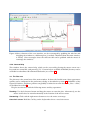
1
Profex
Version 3.2.0
BGMN Backend
June 21, 2014
Contents
1. Introduction
4
2. Installation
5
2.1. Windows . . . . . . . . . . . . . . . . . .
2.1.1. Profex-BGMN bundle . . . . . .
2.2. Linux . . . . . . . . . . . . . . . . . . . .
2.2.1. Getting the source . . . . . . . .
2.2.2. Disabling Bruker BRML support
2.2.3. Compiling from source code . .
2.3. Mac OS X . . . . . . . . . . . . . . . . . .
.
.
.
.
.
.
.
.
.
.
.
.
.
.
.
.
.
.
.
.
.
.
.
.
.
.
.
.
.
.
.
.
.
.
.
.
.
.
.
.
.
.
.
.
.
.
.
.
.
.
.
.
.
.
.
.
.
.
.
.
.
.
.
.
.
.
.
.
.
.
.
.
.
.
.
.
.
.
.
.
.
.
.
.
.
.
.
.
.
.
.
.
.
.
.
.
.
.
.
.
.
.
.
.
.
.
.
.
.
.
.
.
.
.
.
.
.
.
.
.
.
.
.
.
.
.
.
.
.
.
.
.
.
.
.
.
.
.
.
.
.
.
.
.
.
.
.
.
.
.
.
.
.
.
.
.
.
.
.
.
.
.
.
.
.
.
.
.
.
.
.
.
.
.
.
.
.
.
.
.
.
.
3. Setup
3.1. Automatic setup . . . .
3.1.1. Windows . . . .
3.1.2. Linux . . . . . .
3.1.3. Mac OS X . . .
3.2. Manual setup . . . . .
3.3. Using WINE on Linux
5
5
5
5
6
6
6
7
.
.
.
.
.
.
.
.
.
.
.
.
.
.
.
.
.
.
.
.
.
.
.
.
.
.
.
.
.
.
.
.
.
.
.
.
.
.
.
.
.
.
.
.
.
.
.
.
.
.
.
.
.
.
.
.
.
.
.
.
.
.
.
.
.
.
.
.
.
.
.
.
.
.
.
.
.
.
.
.
.
.
.
.
.
.
.
.
.
.
.
.
.
.
.
.
.
.
.
.
.
.
.
.
.
.
.
.
.
.
.
.
.
.
.
.
.
.
.
.
.
.
.
.
.
.
.
.
.
.
.
.
.
.
.
.
.
.
.
.
.
.
.
.
.
.
.
.
.
.
.
.
.
.
.
.
.
.
.
.
.
.
.
.
.
.
.
.
.
.
.
.
.
.
.
.
.
.
.
.
.
.
.
.
.
.
.
.
.
.
.
.
.
.
.
.
.
.
.
.
.
.
.
.
.
.
.
.
.
.
.
.
.
.
.
.
4.1. User Interface Elements . . . . . . . .
4.2. Dockable windows . . . . . . . . . . .
4.2.1. Projects . . . . . . . . . . . . . .
4.2.2. Plot options . . . . . . . . . . .
4.2.3. Refinement protocol . . . . . .
4.2.4. Global Parameters and GOALs
4.2.5. Local Parameters . . . . . . . .
4.2.6. Context Help . . . . . . . . . .
4.3. The Plot area . . . . . . . . . . . . . . .
4.4. Tool bars . . . . . . . . . . . . . . . . .
.
.
.
.
.
.
.
.
.
.
.
.
.
.
.
.
.
.
.
.
.
.
.
.
.
.
.
.
.
.
.
.
.
.
.
.
.
.
.
.
.
.
.
.
.
.
.
.
.
.
.
.
.
.
.
.
.
.
.
.
.
.
.
.
.
.
.
.
.
.
.
.
.
.
.
.
.
.
.
.
.
.
.
.
.
.
.
.
.
.
.
.
.
.
.
.
.
.
.
.
.
.
.
.
.
.
.
.
.
.
.
.
.
.
.
.
.
.
.
.
.
.
.
.
.
.
.
.
.
.
.
.
.
.
.
.
.
.
.
.
.
.
.
.
.
.
.
.
.
.
.
.
.
.
.
.
.
.
.
.
.
.
.
.
.
.
.
.
.
.
.
.
.
.
.
.
.
.
.
.
.
.
.
.
.
.
.
.
.
.
.
.
.
.
.
.
.
.
.
.
.
.
.
.
.
.
.
.
.
.
.
.
.
.
.
.
.
.
.
.
.
.
.
.
.
.
.
.
.
.
.
.
.
.
.
.
.
.
.
.
.
.
.
.
.
.
.
.
.
.
.
.
.
.
.
.
.
.
.
.
.
.
.
.
.
.
.
.
.
.
4. Main Window
7
7
7
8
8
9
10
1
10
11
12
12
12
12
12
13
13
14
5. Menu Structure
5.1.
5.2.
5.3.
5.4.
5.5.
5.6.
5.7.
File . . . .
Edit . . . .
View . . .
Run . . . .
Instrument
Window .
Help . . .
15
.
.
.
.
.
.
.
.
.
.
.
.
.
.
.
.
.
.
.
.
.
.
.
.
.
.
.
.
.
.
.
.
.
.
.
.
.
.
.
.
.
.
.
.
.
.
.
.
.
.
.
.
.
.
.
.
.
.
.
.
.
.
.
.
.
.
.
.
.
.
.
.
.
.
.
.
.
.
.
.
.
.
.
.
.
.
.
.
.
.
.
.
.
.
.
.
.
.
.
.
.
.
.
.
.
.
.
.
.
.
.
.
.
.
.
.
.
.
.
.
.
.
.
.
.
.
.
.
.
.
.
.
.
.
.
.
.
.
.
.
.
.
.
.
.
.
.
.
.
.
.
.
.
.
.
.
.
.
.
.
.
.
.
.
.
.
.
.
.
.
.
.
.
.
.
.
.
.
.
.
.
.
.
.
.
.
.
.
.
.
.
.
.
.
.
.
.
.
.
.
.
.
.
.
.
.
.
.
.
.
.
.
.
.
.
.
.
.
.
.
.
.
.
.
.
.
.
.
.
.
.
.
.
.
.
.
.
.
.
.
.
.
.
.
.
.
.
.
.
.
.
.
.
.
.
.
.
.
.
.
.
.
.
.
.
.
.
.
.
.
.
.
.
.
.
.
.
.
.
.
.
.
.
.
.
.
.
.
.
.
.
.
.
.
.
.
.
.
.
.
.
6.1. General . . . . . . . . . . . . . . . .
6.1.1. Editor . . . . . . . . . . . .
6.1.2. Appearance and Behaviour
6.1.3. Reference Structures . . . .
6.2. Graphs . . . . . . . . . . . . . . . .
6.2.1. General Appearance . . . .
6.2.2. Fonts . . . . . . . . . . . . .
6.2.3. Scan Styles . . . . . . . . . .
6.3. BGMN . . . . . . . . . . . . . . . .
6.3.1. Configuration . . . . . . . .
6.3.2. STR File Handling . . . . .
6.3.3. CIF File Handling . . . . . .
6.3.4. Summary Table . . . . . . .
6.4. Fullprof . . . . . . . . . . . . . . . .
.
.
.
.
.
.
.
.
.
.
.
.
.
.
.
.
.
.
.
.
.
.
.
.
.
.
.
.
.
.
.
.
.
.
.
.
.
.
.
.
.
.
.
.
.
.
.
.
.
.
.
.
.
.
.
.
.
.
.
.
.
.
.
.
.
.
.
.
.
.
.
.
.
.
.
.
.
.
.
.
.
.
.
.
.
.
.
.
.
.
.
.
.
.
.
.
.
.
.
.
.
.
.
.
.
.
.
.
.
.
.
.
.
.
.
.
.
.
.
.
.
.
.
.
.
.
.
.
.
.
.
.
.
.
.
.
.
.
.
.
.
.
.
.
.
.
.
.
.
.
.
.
.
.
.
.
.
.
.
.
.
.
.
.
.
.
.
.
.
.
.
.
.
.
.
.
.
.
.
.
.
.
.
.
.
.
.
.
.
.
.
.
.
.
.
.
.
.
.
.
.
.
.
.
.
.
.
.
.
.
.
.
.
.
.
.
.
.
.
.
.
.
.
.
.
.
.
.
.
.
.
.
.
.
.
.
.
.
.
.
.
.
.
.
.
.
.
.
.
.
.
.
.
.
.
.
.
.
.
.
.
.
.
.
.
.
.
.
.
.
.
.
.
.
.
.
.
.
.
.
.
.
.
.
.
.
.
.
.
.
.
.
.
.
.
.
.
.
.
.
.
.
.
.
.
.
.
.
.
.
.
.
.
.
.
.
.
.
.
.
.
.
.
.
.
.
.
.
.
.
.
.
.
.
.
.
.
.
.
.
.
.
.
.
.
.
.
.
.
.
.
.
.
.
.
.
.
.
.
.
.
.
.
.
.
.
.
.
.
.
.
.
.
.
.
.
.
.
.
.
.
.
.
.
.
.
.
.
.
.
.
.
.
.
.
.
.
.
.
.
.
.
.
.
.
.
6. Preferences
15
16
16
17
17
17
17
19
7. Structure and Device Database
19
19
19
19
20
20
20
21
21
21
22
23
23
23
24
7.1. Structure Template Files . . . . . . . . . . . . . . . . . . . . . . . . . . . . . . . . . . . 24
7.2. STR File Handling . . . . . . . . . . . . . . . . . . . . . . . . . . . . . . . . . . . . . . . 24
7.3. Device Configuration Files . . . . . . . . . . . . . . . . . . . . . . . . . . . . . . . . . . 26
8. ,,Add Phase” dialog
28
8.1. Project organization . . . . . . . . . . . . . . . . . . . . . . . . . . . . . . . . . . . . . . 28
9. Exporting data
9.1. Graphs . . . . . . . . . . . . . . . . . .
9.1.1. ASCII free format (XY) . . . . .
9.1.2. Pixel image (PNG) . . . . . . .
9.1.3. Gnuplot (GPL) . . . . . . . . .
9.1.4. Scalable vector graphics (SVG)
9.2. Printing to PDF . . . . . . . . . . . . .
9.3. Refinement results . . . . . . . . . . .
31
.
.
.
.
.
.
.
.
.
.
.
.
.
.
.
.
.
.
.
.
.
.
.
.
.
.
.
.
.
.
.
.
.
.
.
.
.
.
.
.
.
.
.
.
.
.
.
.
.
.
.
.
.
.
.
.
.
.
.
.
.
.
.
.
.
.
.
.
.
.
.
.
.
.
.
.
.
.
.
.
.
.
.
.
.
.
.
.
.
.
.
.
.
.
.
.
.
.
.
.
.
.
.
.
.
.
.
.
.
.
.
.
.
.
.
.
.
.
.
.
.
.
.
.
.
.
.
.
.
.
.
.
.
.
.
.
.
.
.
.
.
.
.
.
.
.
.
.
.
.
.
.
.
.
.
.
.
.
.
.
.
.
.
.
.
.
.
.
.
.
.
.
.
.
.
.
.
.
.
.
.
.
.
.
.
.
.
.
.
31
31
31
32
32
33
33
10. Scan batch conversion
34
11. CIF import
35
11.1. Automatic conversion of thermal displacement parameters . . . . . . . . . . . . . . . 35
2
12. Instrument configurations
39
13. First steps
41
14. Scan File Handling
42
A. Bundle File Structure
49
A.1. Windows . . . . . . . . . . . . . . . . . . . . . . . . . . . . . . . . . . . . . . . . . . . . 49
A.2. Mac OS X . . . . . . . . . . . . . . . . . . . . . . . . . . . . . . . . . . . . . . . . . . . . 49
A.3. Linux . . . . . . . . . . . . . . . . . . . . . . . . . . . . . . . . . . . . . . . . . . . . . . 50
Index
52
3
1. Introduction
Profex is a graphical user interface for Rietveld refinement of powder X-ray diffraction data. It
supports two different Rietveld backends BGMN [1] and FullProf.2k [2]. Profex does not perform
any refinement calculations, but it simplifies the use of the Rietveld backends in many ways:
• It displays diffraction patterns.
• It converts pattern files to formats supported by the backends.
• It simplifies setting up control files with databases for crystal structures and instrument
configurations.
• It handles file names.
• It summarizes the results and supports export to CSV file format.
• It supports batch processing and parallel processing of several datasets at a time.
Profex runs on Windows, Linux, and Mac OS X operating systems and is available as free software licensed under the GNU General Public License (GPL) version 2 or any later version. The
latest version can be downloaded from [3].
4
2. Installation
2.1. Windows
2.1.1. Profex-BGMN bundle
Since Profex requires a Rietveld refinement backend, a bundle containing both Profex and BGMN
is offered for download on the Profex website. Using the bundle is the preferred way of installation if no previous installation is present on the computer. The directory and file structure of the
bundle is shown in appendix ??. The software does not need installation. The downloaded archive
can be extracted to any location on the computer. Automatic configuration of Profex will be able
to locate the BGMN installation if the relative paths of the BGMNwin and Profex-3.2.0 folders are
maintained. Therefore, it is recommended to copy the entire bundle to the same location on the
hard disk, as shown in Fig. 1. Follow these instructions to install BGMN and Profex:
1. Download Profex-BGMN-Bundle-3.2.0.zip from [3]
2. Extract the bundle to your harddisk (e. g. C:\Program Files)
3. Run Profex by executing the file profex.exe (e. g. C:\Program Files\Profex-3.2.0\profex.exe)
The file and directory structure of the bundle is explained in appendix A. Profex is also available for download without BGMN. This is the preferred way of installation if BGMN is already
installed on the computer, or if previous versions of Profex are to be upgraded. The Profex binary
archive does not need installation. Extracting the archive to the local hard drive is sufficient.
If a previous version is installed on the same computer, using a new version will not interfere
with the existing installation. Old and new versions can be used at the same time, they will share
the configuration options.
2.2. Linux
A binary archive of BGMN for Linux (i686) is available for download on the Profex website [3].
Profex, however, must be compiled from source. It requires a C++ compiler environment and
the Qt toolkit version 4 or 5 to be installed [4], including header files. Qt version 5.2 or later is
recommended. For Qt5 the following modules and header files must be installed:
widgets , xml , p r i n t s u p p o r t , s c r i p t , svg
Support for Bruker BRML raw data files requires an additional dependency. The QuaZIP library
and header files [5] version 0.4.1 or later must be installed. By default, the Profex source code is
configured to include support for BRML files.
2.2.1. Getting the source
Download the source code archive profex-3.2.0.tar.gz from the Profex website [3], extract it to your
harddisk and navigate into the source code directory:
t a r xzvf profex − 3 . 2 . 0 . t a r . gz
cd profex − 3 . 2 . 0
5
C:\Program Files
BGMNwin
Profex-3.2.0
Structures
Devices
Profex-BGMN-Bundle-3.2.0.zip
BGMNwin
Profex-3.2.0
Structures
Devices
(a) Structure of the bundle archive.
(b) Structure on the hard disk.
Figure 1: When extracting the Profex-BGMN-Bundle to the hard disk, automatic setup will only be
successful if the BGMNwin and Profex-3.2.0 directories are copied to the same location.
2.2.2. Disabling Bruker BRML support
If BRML support is disabled, Profex only depends on the Qt toolkit. To disable BRML support
open the file Profex2.pro in a text editor and change the line
DEFINES += QUAZIP
to
DEFINES −= QUAZIP
Save the file and proceed with the compilation.
2.2.3. Compiling from source code
Run the following commands from the source code directory:
qmake P r o f e x 2 . pro
make − j 4
./ profex
If error messages occur and the program does not start after typing ./profex, read the error
messages carefully and try to solve all dependency and version problems with your distribution’s
software repository.
2.3. Mac OS X
A disk image containing Profex and BGMN for Mac OS X 10.6.8 or newer is provided for download on the Profex website [3]. The binary requires a 64bit CPU. Visit [6] to find out whether a
specific Apple computer uses a 64bit or a 32bit CPU.
Mount the disk image and drag the folder Profex-BGMN to the Applications folder. The file and
directory structure of the bundle is explained in appendix A. Then run the application ,,ProfexBGMN/profex”. The automatic setup routine (section 3) will find the BGMN installation and the
structure and device directories.
6
3. Setup
3.1. Automatic setup
When starting Profex for the first time, the program will try to locate the BGMN installation directory and structure and device database directories automatically. Automatic configuration will
also be executed later if the configured paths are invalid. It is therefore possible to force automatic
setup later by deleting the paths to BGMN and the database directories in the preferences dialog.
Automatic setup is platform specific. The locations scanned automatically are listed below.
3.1.1. Windows
Two directories named ,,Structures” and ,,Devices” are expected to be located in the directory of
,,profex.exe”. ,,BGMN.EXE” is expected to be found in a directory called BGMNwin stored next
to the parent directory of ,,profex.exe”, i. e. at:
• <location of profex.exe>\..\BGMNwin\BGMN.EXE.
3.1.2. Linux
On Linux, a list of directories is scanned for the executable file ,,bgmn”. Scanning will stop at the
first match. The directories are scanned in the following order:
1. /home/<user>/BGMN/
2. /home/<user>/BGMNwin/
3. /opt/bgmnwin/
4. /opt/bgmn/
5. /opt/BGMNwin/
6. /usr/bin/
7. /usr/local/bin/
Directories named ,,Structures” and ,,Devices” will be searched in the following order at:
1. /home/<user>/Structures
/home/<user>/Devices
2. /home/<user>/BGMN-Templates/Structures
/home/<user>/BGMN-Templates/Devices
3. /opt/Structures
/opt/Devices
4. /opt/BGMN-Templates/Structures
/opt/BGMN-Templates/Devices
7
3.1.3. Mac OS X
On Mac OS X the BGMN installation and Structures and Devices directories will be scanned relative to the path of the Profex application bundle. Profex expects to find the following files, starting
at the position of the Profex application bundle:
• <location of profex.app>/../BGMNwin/bgmn
• <location of profex.app>/../BGMN-Templates/Structures
• <location of profex.app>/../BGMN-Templates/Devices
3.2. Manual setup
The following sections describe how to configure Profex to find the BGMN backend, as well as
the structure and device database directories manually. There are some scenarios when automatic
setup will fail and the backend and database directories are not found, or when the automatic
configuration is not desired:
• if only Profex was downloaded instead of a Profex-BGMN bundle
• if the Profex and BGMN folders from the bundle were not copied to the same location on the
harddisk
• if Profex is supposed to use existing BGMN and structure/device databases rather than the
ones downloaded with the bundle
• on Linux no bundles are available
In these cases, manual configuration is necessary. Follow these instructions to set up Profex
manually:
1. Run Profex and go to ,,Edit → Preferences . . . ”.
2. On the page ,,General” set the ,,Default Project Type” to ,,BGMN” (Fig. 2).
3. Go to page ,, BGMN”. On the tab ,,Configuration” check the configuration of ,,BGMN Backend”. If auto-detection was successful, the lines for executable files and files directories are
not empty (Fig. 2).
4. If the lines are empty, click the button on the right of each line and navigate to the corresponding executable file. The file names depend on the operating system.On Windows, the
files are called BGMN.EXE, MAKEGEQ.EXE, GEOMET.EXE, OUTPUT.EXE and GERTEST.EXE.
On Linux and Mac OS X these files are called bgmn, makegeq, geomet, output, and
gertest.
8
(a) Set the default project type to BGMN.
(b) Select the BGMN executable files, as well as
Structure and Device database directories.
Figure 2: Manual configuration of the BGMN backend in Profex.
3.3. Using WINE on Linux
Profex supports running the Windows version of BGMN on Linux using WINE. In that case, a
,,BGMNwin” directory from a Windows installation can be copied to any location on a Linux
system. The executable files of the BGMN backend will then be called BGMN.EXE, MAKEGEQ.EXE,
GEOMET.EXE, OUTPUT.EXE, and GERTEST.EXE. Checking the box ,,Run in WINE” and entering
the WINE executable in the configuration dialog (Fig. 2), which is usually /usr/bin/wine, will
let Profex call the BGMN backend in WINE. However, for performance reasons it is recommended
to use the native Linux version of BGMN if available.
9
4. Main Window
The program’s main window features a menu bar and several tool bars to access all functions and
settings (Fig. 3). The central area of the main window is occupied by the plot area, and optionally
one or several text editors, which are accessible by tabs at the top of the plot area. The plot area
cannot be closed, but text editors can be closed by clicking the close button on their tab.
The central area is surrounded by several dockable windows showing additional information
and giving access to more features. These dockable windows can be closed and opened from the
,,Window” menu. They can also be re-arranged (Fig. 4) by clicking on the title bar showing the
window’s name, and dragging it to another location. Dockable windows can be stacked on top of
each other to hide less frequently used windows, or detached from the main window, e. g. to be
placed on another screen, or closed.
4.1. User Interface Elements
The following list explains the elements of the user interface shown in Fig. 3 in more detail.
1 Menu bar gives access to most features, as well as the program’s preferences. All menu items
are discussed in section 5.
2 Main tool bar gives access to file operating features such as opening, saving, etc.
3 Project tool bar gives access to project related functions, such as opening/closing structure
files, exporting results, adding/removing phases etc.
4 Refinement tool bar gives access to starting/stopping refinements or batch refinements.
5 Reference structure tool bar allows to select reference structures to display hkl indices, as well
as to start scanning and indexing new structure files. See section 4.4 for more information.
6 Plot area displays raw or refined scans, and opens text editors for control files, results files,
structure files, or generic text files.
7 Projects window lists all open projects and the refinement status. Selecting a project from this
list will show it in the central plot area.
8 Plot options lists all scans loaded in the plot area. The ,,Show” checkbox can be used to
show/hide certain scans to customize the appearance of the plot.
9 Refinement protocol shows output generated by the refinement backend.
10 Global Parameters and GOALs shows a summary table of refined global parameters. Listing
EPS parameters can be configured in the program’s preferences dialog.
11 Local Parameters and GOALs shows a summary table of refined local parameters. The pa-
rameters shown here can be customized in the program’s preferences dialog.
12 Context help shows the context help text when pressing ,,F1” on a keyword in a control file.
13 Status bar shows various information such as mouse cursor coordinates on the graph, and the
wavelength used to transform 2θ angles to d values.
10
Figure 3: The Profex main window. Elements 1–13 are described in section 4.1.
4.2. Dockable windows
All windows arranged around the central plot and editor area (no. 7–12 in Fig. 3) can be rearranged or closed to match the user’s preferences. They are called dockable windows, because
they can be docked to different areas of the main window. Some examples are shown in Fig. 4 and
explained below:
Moving: Grab the dockable window at it’s title bar (e. g. the bar (green rectangles on Fig. 4) and
drag it to a different location. If the window can be docked, the area will be highlighted.
Stacking: Drag the dockable window onto another dockable window. The dragged window will
be stacked on top. Tab buttons will automatically appear to give access to both windows.
Unlimited numbers of windows can be stacked.
Detaching: Drag a window outside of the main window and release it when no dockable area is
highlighted. The window is now detached from the main window and floating freely on the
screen. Use this configuration to place windows on a second screen. Detached windows can
also be stacked. Drag the detached window back into the main window to dock it.
Closing / Opening: Dockable windows can be closed by clicking on the close button (x) in the title
bar. To open it again, use the menu ,,Window” in the main window’s menu bar.
11
4.2.1. Projects
This list shows all open projects and their current status. Click on a project to view it in the plot
and editor area. Most actions from the menu and toolbar will apply to the currently shown project.
Projects can be edited while another project is refining. Multiple projects can be refined at a
time, but refinement may be slow depending on CPU power and number of CPU cores.
Running a batch refinement (see section 5.4) will allow to refine all open projects in a sequence,
rather than parallel.
4.2.2. Plot options
This list shows all scans loaded in the currently shown project. To change the scans’ drawing style
(color, line style, line width), refer to the graph preferences discussed in section 6.2. Names of
scans cannot be changed, they depend on the names read from the scan files.
Visibility of each scan can be changed by checking or unchecking the box in front of the scan
name. For refined scans Profex distinguishes between main scans (usually Iobs , Icalc , Idi f f , and the
background curve), as well as phase patterns. All phase patterns can be toggled on or off at once
by using the function ,,View → Show/Hide phase patterns”. This change is persistent and applies
to all open projects. It is a convenience function for easy showing or hiding all phase patterns, but
the same result can be obtained by manually checking or unchecking all phase patterns of all open
projects.
hkl tick marks are considered as part of phase patterns. Showing/hiding a phase pattern will
also show or hide the phase’s hkl lines. By using the functions in ,,View → Plot” (see section 5.3),
drawing of hkl lines and phase patterns can be controlled separately. This allows to draw either
no phase information, hkl lines only, phase patterns only, or both.
4.2.3. Refinement protocol
This windows shows the output of the Rietveld refinement backend.
4.2.4. Global Parameters and GOALs
At the end of the refinement, this window shows a summary of the refinement results. The displayed parameters depend on the Rietveld refinement backend. For BGMN, the table shows
all global goals and parameters, including estimated standard deviations (ESD) as calculated by
BGMN. Some configuration options are available in the preferences as described in section 6.3.4.
Values summarized here can also be exported to a CSV table using the function ,,File → Export
Global Parameters and GOALs (Ctrl+E)” (see section 5.1).
4.2.5. Local Parameters
At the end of the refinement, this window shows a summary of refined local (phase related) parameters. This function depends on the Rietveld refinement backend and is not available for all
backends. In case of BGMN, is is available and can be configured in the preferences as described
in section 6.3.4. Values summarized here can also be exported to a CSV table using the function
,,File → Export Local Parameters” (see section 5.1).
12
Figure 4: Many elements of the user interface can be re-arranged by grabbing the title bar and
dragging the window to a different place (1 stacked; 2 detached from the main window;
3 closed). Green rectangles show the title bars that can be grabbed with the mouse to
rearrange the windows.
4.2.6. Context Help
This window shows the context help, which can be accessed by placing the mouse cursor on a
keyword in a control file, and pressing ,,F1”. Context help is available for BGMN, but may not be
available for other Rietveld refinement backends (see section 5.7).
4.3. The Plot area
The plot area is the central area of the main window. It shows the loaded scans. Some appearance
options can be configured in the preferences dialog as described in section 6.2. Visibilities of the
legend, hkl indices, and phase patterns can globally switched on or off in the menu ,,View → Plot”,
as described in section 5.
The plot area interacts with the following mouse and key operations:
Zooming: Use the left mouse button and drag the mouse to zoom the plot. Alternatively, use the
mouse scroll wheel to zoom horizontally to the location of the mouse cursor.
Unzooming: Click with the right mouse button to view the entire scan range.
Cross hair cursor: Hold the Ctrl key on the keyboard to show a cross hair cursor.
13
Counting noise cursor: Hold the Shift key on the keyboard to show a cursor indicating a range
of
±p
1
Intensity[counts]
This range represents the statistical counting noise and allows to evaluate mismatches between Iobs and Icalc , for example at the tips of peaks.
Double click with left mouse button: This will load the reference structure with it’s strongest
peak closest to the double click position. This is a very primitive way of phase identification,
however, it can be very efficient and useful in some situations. Note that only indexed structure files are considered. Refer to section 4.4 for more information on indexing of references
structure files. Also note that the strongest peak of the reference structure indices depends
on the instrument configuration used for indexing (FDS vs. ADS) and may therefore not be
at the location of the currently processed scan.
4.4. Tool bars
All functions shown in the main toolbar, project toolbar, and refinement toolbar are also accessible
in the menu bar and are described in detail in section 5. Toolbars can be re-arranged by dragging
the left end to another position, or shown / hiden by right-clicking on a toolbar and checking or
unchecking the toolbar in the context menu.
Elements of the reference structure toolbar are only visible if at least one project is loaded. They
are not accessible through a menu, only by the toolbar buttons:
Reference structures: A menu allowing to select a reference structure from all STR files found
in the structure database directory. If selected, the STR file’s hkl lines will be shown in the
graph. This is a generic way of phase identification. When using the ,,Add Phase” dialog
while a reference structure is displayed, this structure file will be pre-selected in the ,,Add
Phase” dialog.
If STR files have not been indexed before, hkl indices will be calculated on the fly when the
structure is selected. On modern computers, this only takes a second or two. Afterwards
the hkl positions will be buffered and be available instantly. The buffer can be cleared as
described in section 6.1.3. Note that the double-click function described in section 4.3 is only
available for indexed reference structures.
Reset reference structure: This button will reset the reference structure dropdown menu and
hide reference hkl lines. After resetting, no structure will be pre-selected in the ,,Add Phase”
dialog anymore.
Search and index new reference structures: Pressing this button will scan the structure database
directory for new STR files and index all new files. The reference structures become immediately available in all projects.
14
5. Menu Structure
5.1. File
Open Text File. . . (Ctrl+O) Opens a file in a text editor. If a project with the same name as the
text file’s base name is already open, the file is opened in this project. Else a new project is
created.
If the text file is a control or results file, Profex will automatically locate all other control and
results files of the same project, as well as the scan file, and open them, too. Non-existing
files are ignored.
BGMN structure files (*.str) are always opened in the currently shown project, regardless of
the project name.
Open Graph File. . . (Ctrl+G) Opens a scan file in the graph page. If a control and/or results file
with the same base name is found, Profex will open it, too.
Close Project (Ctrl+W) Closes the current project.
Save (Ctrl+S) Saves the current file under the same file name. This function only works for text
files.
Save file as. . . (Shift+Ctrl+S) Saves the current file under a new file name. A file dialog is shown
to ask for the file name, location, and file format.
For scan files, different output formats can be selected. Scans can be saved as raw data for
further processing, or images.
Print (Ctrl+P) Prints the currently shown text or graph file. Printing options may differ depending
on the platform and device driver.
Open all project STR files Opens all BGMN structure files (*.str) referenced in the current
project’s control file (*.sav) in new pages.
Close all project STR files Closes all BGMN structure files (*.str) shown in the current project.
Import CIF. . . Opens a dialog to convert CIF files (*.cif) to BGMN structure files (*.str). See section
11 for more information.
Scan Batch Conversion. . . Opens a dialog for batch conversion of graph files. All currently
opened project scans will be added to the batch list by default. More files can be added
or deleted in the dialog. See section 10 for more information.
Export Global Parameters and GOALs (Ctrl+E) Exports the global parameters and goals (e. g.
phase quantities) to a semicolon separated spread sheet (*.csv). See section 9.3 for more
information.
Export Local Parameters and GOALs (Shift+Ctrl+E) Exports the local parameters and goals (e. g.
structural parameters) to a semicolon separated spread sheet (*.csv). See section 9.3 for more
information.
Quit (Ctrl+Q) Quits the application.
15
5.2. Edit
Undo Reverts the last change in the currently shown text file.
Redo Restores the last undone change in the currently shown text file.
Copy Control File Copies the current project’s control file to other projects and adapts all input
and output file names to match the projects’ base names. A dialog will allow to select which
projects’ control file shall be modified. Existing control files will be overwritten.
Note that this function does not check whether referenced structure files are actually present
in all project directories. It only manages control files, but not structure files.
Reset File Reverts the current project’s control file to the state before the last refinement. This
function is only used for the Fullprof.2k backend, but not for BGMN, because BGMN usually
does not modify STR and SAV files.
Add Phase. . . (F8) Opens a dialog to create a control file by selecting an instrument configuration
and phases (crystal structure files).
If a phase is activated in the Reference Phase box, it will be preselected in the Add Phase
dialog.
The option to create a default control file is automatically activated or deactivated, depending on whether or not a control file already exists.
If a default control file is created despite an existing control file, the existing one will be
overwritten, any previously added modifications or phases will be lost.
Selected structure files and instrument configuration files will be copied from the structure
and device database directory to the project directory. Files already existing in the destination directory will be skipped. If the option ,,overwrite existing files” is checked, existing
structure files will be overwritten with the file copied from the structure file database. See
section 8 for more information.
Remove Phase. . . Removes a phase from the control file. Optionally, the structure file will be
deleted. Deleting structure files may cause problems with other projects stored in the same
directory and accessing the same structure files.
Preferences. . . Opens the program’s preferences dialog. All preference options are discussed in
detail in section 6.
5.3. View
Switch to Graphs (Ctrl+1) Raises the Graph page of all projects.
Switch to Control Files (Ctrl+2) Raises page 2 (usually the control file) of all projects.
Switch to Output Files (Ctrl+3) Raises page 3 (usually the results file) of all projects.
Set Zoom Range. . . Opens a dialog to zoom the graph to precise upper and lower limits for angle
and intensity.
16
Show/Hide Phase Patterns (Ctrl+0) Activates or deactivates visibility of all phases. This option
applies to all open projects. It only checks or unchecks the visibility boxes of all phase patterns in the Plot Options list for convenient displaying or hiding of all phases. Individual
phases can be shown or hidden by selecting or un-selecting the ,,show” option in the Plot
Options list. More information is given in section 4.2.2.
Plot Configure the visibility of the following elements on the plot:
Phase Patterns Shows or hides patterns of phases.
Legend Shows or hides the plot legend.
hkl Indices Shows or hides the hkl index tick marks at the top of the plots.
5.4. Run
Run Refinement (F9) Starts the refinement of the currently shown project.
Abort (Ctrl+C) Aborts refinement of the currently shown project. In batch refinement mode, all
running and scheduled refinements will be aborted.
Run Batch Refinement (F10) Starts a batch refinement of all open projects.
5.5. Instrument
Edit Configuration. . . Opens a dialog to process BGMN instrument configurations. See section
12 for more information.
5.6. Window
Projects Shows or hides the Projects list window.
Plot Options Hows or hides the Plot Options window.
Refinement Protocol Shows or hides the Refinement Protocol window.
Global Parameters and GOALs Shows or hides the summary table window for global parameters
and goals.
Local Parameters Shows or hides the summary table window for local parameters and goals.
Context Help Shows or hides the context help display.
5.7. Help
Context Help. . . (F1) Shows the context help of the keyword under the text cursor. The ,,Context
Help” window (,,View” menu) must be shown to display the context help.
BGMN Variables. . . Opens a web browser showing the BGMN variables documentation page.
BGMN SPACEGRP.DAT. . . Opens a dialog to browse spacegroups and atomic positions sup-
ported by BGMN.
17
About Profex. . . Shows information about Profex.
18
6. Preferences
6.1. General
6.1.1. Editor
Font Sets the font of the text editor and refinement protocol window.
6.1.2. Appearance and Behaviour
Default Project Type For files not specific for either BGMN or Fullprof.2k, this option determines
which type of project will be created when such a file is opened. The file type is identified
by the file extension.
File extensions can also be associated with either of the two backends by adding the extension either to the list of ,,File Extensions associated with BGMN” or ,,File Extensions associated with Fullprof” on the corresponding backend configuration pages of the preferences
dialog.
Toolbar Layout Select how icons and text in Profex’ toolbars are shown.
Multi-Scan Files Select whether multi-range files will be shown as individual scans, as the sum
of all ranges, or as the average of all ranges.
Default Wavelength This wavelength, given in Å, is used for scan files not containing any infor-
mation about the wavelength.
Always use default Wavelength If checked, Profex will ignore the wavelength read from the scan
file and always use the default wavelength to calculate d values from diffraction angles.
6.1.3. Reference Structures
Automatically index new structure files If checked, Profex will scan the structure file directory
for new structure files each time Profex is started and the first project is loaded.
If not checked, new structures will be indexed the first time they are selected in the Reference
Structures box.
Structures will not be available for double-click phase identification as long as they have not
been indexed.
Clear Buffer Clears the buffer file with structure file hkl indices. Profex must be restarted for this
to take effect. All structure files will be re-indexed either automatically, or when selected
from the Reference Structures box.
Calculate hkl positions in range Specifies the lower and upper 2θ angle for hkl indices to be cal-
culated. Larger ranges will require more time to index. The range may be smaller or larger
than scan file ranges.
19
6.2. Graphs
6.2.1. General Appearance
Use AntiAliasing for Graphs (slow!) Uses anti aliasing to draw the plots. If checked, lines look
smoother but also wider. Drawing will be slower if checked.
Update Graph after each Cycle If checked, the plots will be updated continuously during the re-
finement. If not checked, they will remain static and only be updated at the end of the
refinement.
Updating the graph takes some time. For very long refinements or batch refinements deactivating this option may save some time. For normal operation it is recommended to activate
this option.
Display Line Width Width in pixels of all lines (plots, axes, tick marks) of the graph on computer
screens.
Printing Line Width Width in points of all lines (plots, axes, tick marks) of the graph on printouts.
This value should usually be greater than the display line width.
Symbol Size Size of the measured data points when not using solid lines (e. g. dots or crosses) in
pixels.
Y-axis Scaling Scaling of the y-axis. Options are linear, logarithmic with a base of 10 (log10), or
square root (sqrt).
Color of Reference hkl Lines Color of the hkl lines when selecting a reference structure from the
Reference Structures box.
Create Thumbnail If checked, a thumbnail picture of the refined plot will be created at
the end of the refinement. This file is stored in the project directory with the name
project-basename tn.png. It allows easy browsing of refined projects. The width
of the picture can be specified in pixels. The height is calculated from the displayed aspect
ratio.
Show Texture of hkl Lines (if available) If checked, the box appearing when pointing the mouse
cursor on hkl index tick marks on the plot also shows the texture factor.
6.2.2. Fonts
Font Title Select the font of the file name at the top-right of the graph.
Font Axis Labels Select the font of the graph axis labels.
Font Tick Marks Select the font of the graph tick marks.
Font Legend Select the font of the graph legend.
20
6.2.3. Scan Styles
Color Customize the list of colors to be used to draw scans by double-clicking on the color cell. If
more scans are loaded than colors are available from the list, a random color will be created
and added to the list. It can be changed manually later. Line widths can be changed on the
Graph’s General Appearance page.
Point Style Select the style to draw scans. ,,Solid” draws the scan as a solid line. ,,Points” draws a
dot at the measured position, ,,Cross” draws a cross at the measured position. Symbol sizes
of crosses and points can be changed on the Graph’s General Appearance page.
+ Add another color to the color list.
− Remove the currently selected color from the list.
6.3. BGMN
6.3.1. Configuration
BGMN Backend
BGMN Executable Select the BGMN executable file. This file is part of the BGMN installation. It
is called BGMN.EXE on Windows, and bgmn on Mac OS X and Linux.
MakeGEQ Executable Select the MakeGEQ executable file. This file is part of the BGMN installa-
tion. It is called MakeGEQ.EXE on Windows, and makegeq on Mac OS X and Linux.
Geomet Executable Select the Geomet executable file. This file is part of the BGMN installation.
It is called GEOMET.EXE on Windows, and geomet on Mac OS X and Linux.
Output Executable Select the Output executable file. This file is part of the BGMN installation. It
is called OUTPUT.EXE on Windows, and output on Mac OS X and Linux.
GERTEST Executable Select the GERTEST executable file. This file is part of the BGMN installa-
tion. It is called GERTEST.EXE on Windows, and gertest on Mac OS X and Linux.
Run in WINE This box is only available on Linux and Mac OS X. It allows to use the Windows
version of BGMN to be run in WINE. Check this option if the executable files specified
above belong to the Windows version of BGMN.
Structure Files Directory Specify the location where BGMN structure files (*.str) are stored.
Device Files Directory Specify the location where BGMN instrument files (*.sav, *.ger, *.geq, *.tpl)
are stored.
File Extensions
File Extensions associated with BGMN These file types will always be opened as BGMN
projects, regardless of the default project type.
21
Convert raw scans to XY format If checked, raw scan files will be converted to ASCII XY free
format (*.xy) prior to starting the refinement.
This option must only be disabled if the raw file format is directly supported by the BGMN
backend (e. g. *.val, *.rd).
Performance
Number of CPU cores used by BGMN Specifies how many CPU cores will be used by BGMN by
adding NTHREADS=n to the control file. ,,Automatic” will use all available cores.
6.3.2. STR File Handling
Custom Profile Function
Use custom profile function Check this option if Profex should automatically change the profile
parameters of BGMN Structure files (*.str). The files will be modified when they are copied
from the structure database to the project directory by calling ,,Edit → Add Phase. . . ”. If this
option is disabled, the profile parameters will not be changed.
Profile Function (RP) Specify the RP=n parameter.
Scaling (GEWICHT) Specify the GEWICHT parameter. Choose SPHARn for refinement of preferred
orientation, or ISOTROPIC for untextured samples.
Lorenzian Size Broadening (B1) Specify B1, enter ANISO for anisotropic crystallite sizes. Check
,,refine” to refine this parameter.
Gaussian Size Broadening (k1) Specify k1. Check ,,refine” to refine this parameter.
Micro Strain (k2) Specify k2, enter ANISO4 for anisotropic micro-strain. Check ,,refine” to refine
this parameter.
GOALs
Add Default Goals Check this option if a set of default goals is to be added to each copied BGMN
Structure file (*.str). Specify the goals in the text field below. Example:
GrainSize(1,1,1) //
Micro-Absorption Correction
Add Correction for Micro-Absorption Check this option if a correction for micro-absorption
(Brindlay correction) shall be added to each copied structure file.
Default Function If checked, the correction formula is hard coded to a default function.
Custom Function Check this line and enter a custom correction function if a correction formula
other than the default one shall be used.
22
6.3.3. CIF File Handling
CIF to STR Conversion
Upper and Lower Limits for Cell Parameters Specifies the range for upper and lower limits of
unit cell parameters to be added automatically to BGMN Structure files (*.str) created from
CIF files.
6.3.4. Summary Table
Output Global Parameters and GOALs
List EPS values If checked, refined EPSn will be shown in the summary table for global parame-
ters and GOALs. Else EPSn parameters will be skipped.
Output Local Parameters
Text Editor Enter the parameters to be read from the local parameters and goals section in the
BGMN List file (*.lst) and shown in the summary table for local parameters and goals. Enter
one parameter per line. The parameters must be written exactly as in the list file, including
case sensitivity.
Reset Pressing this button erases the text field with parameters and inserts a default set of pa-
rameters.
6.4. Fullprof
FullProf.2k options are described in the user manual for Profex using the Fullprof backend.
23
7. Structure and Device Database
Profex supports databases for crystal structures and device configurations for the BGMN backend. These databases are directories containing template files. Profex-BGMN bundles are usually
shipped with default databases. Profex must be configured to find the database directories. Automatic or manual configuration is explained in section 2.
7.1. Structure Template Files
Template files for crystal structures are normal BGMN structure files (*.str) stored at a central
place in the ,,Structures” database directory. The central storage can be placed on a local disk or
on a network share, write access is not required for normal use. When appending a structure file
from the database to a refinement using Profex’s ,,Add Phase” dialog, the file will be copied to the
location of the XRD scan. The original file will never be modified.
The following information is relevant when creating new structure files:
• Use the file extension *.str, other files will be ignored by Profex
• Profex will display the name given after the keyword ,,PHASE=” in the ,,Add Phase” dialog.
• It is recommended to add further information, e. g. an original database code (PDF, AMCSD,
COD) after a comment sign (//) trailing the ,,PHASE=” keyword (see following example).
This text will be shown as a comment in the ,,Add Phase” dialog.
The following lines show an example of the file ,,lime.str”.
PHASE=CaO // 04-007-9734
SpacegroupNo=225 HermannMauguin=F4/m-32/m //
PARAM=A=0.4819_0.4771ˆ0.4867 //
RP=4 k1=0 k2=0 B1=ANISOˆ0.01 GEWICHT=SPHAR2 //
GOAL=GrainSize(1,1,1) //
GOAL:CaO=GEWICHT*ifthenelse(ifdef(d),exp(my*d*3/4),1)
E=CA+2 Wyckoff=a x=0.0000 y=0.0000 z=0.0000 TDS=0.00350000
E=O-2 Wyckoff=b x=0.5000 y=0.5000 z=0.5000 TDS=0.00440000
7.2. STR File Handling
Depending on where structure files are obtained from (created manually, exported from databases,
converted, downloaded, shared with others) they may contain different profile parameters RP, B1,
k1, k2, GEWICHT etc. Altering these files in the structure file database will also affect other users
accessing the same database, and may thus not be desired. Profex offers a feature to modify the
structure files while copying them from the database to the working directory. Choose ,,Edit →
Preferences → BGMN → STR File Handling” to access the settings (Fig. 5). The individual options
on this page are explained in more detail in section 6.3.2.
24
Figure 5: Profex allows to modify structure files automatically to apply custom profile functions
and goals.
25
7.3. Device Configuration Files
For each device configuration Profex expects to find four different files in the device database
directory. These file names are supposed to have the same file name, but different file extensions
(Fig. 6):
*.sav Containing the description of the device configuration. To be processed with GEOMET.
*.ger Containing the raytraced profile shape. To be processed with MAKEGEQ.
*.geq Containing the interpolated profile.
*.tpl A sample *.sav control file for the refinement, not containing any file names or phases.
The *.tpl file is specific to Profex, all other files will be required by BGMN. The *.tpl file can
be any existing refinement control file, but all output file names (LIST=, OUTPUT=, DIAGRAMM=),
all scan file names VAL[n]=, and all structure file names STRUC[n]= should be empty. *.tpl
files allow to add goals, calculations, numbers of threads and similar customizations, which will
be applied by default when creating a new file set from the database. An example is shown
below. All device file names, structure files, scan files, and the various output files will be filled
in automatically by Profex. The automatic processes running in the background when using the
,,Add Phase” dialog are illustrated in Fig. 6. More information on the ,,Add Phase” dialog can be
found in section 8.
% Theoretical instrumental function
VERZERR=
% Wavelength
LAMBDA=CU
% Phases
% Measured data
VAL[1]=
% Minimum Angle (2theta)
% WMIN=10
% Maximum Angle (2theta)
% WMAX=60
% Result list output
LIST=
% Peak list output
OUTPUT=
% Diagram output
DIAGRAMM=
% Global parameters for zero point and sample displacement
EPS1=0
PARAM[1]=EPS2=0_-0.001ˆ0.001
betaratio=0
NTHREADS=2
PROTOKOLL=Y
26
Devices database
Instrument1.tpl
Instrument1.sav
Instrument1.ger
Instrument1.geq
Instrument2.tpl
Instrument2.sav
Instrument2.ger
Instrument2.geq
Instrument3.tpl
Structures database
Albite.str
Barite.str
Calcite.str
Dolomite.str
Ettringite.str
Fluorite.str
Gypsum.str
Hematite.str
Illite.str
Jade.str
Kaolinite.str
Lime.str
Magnesite.str
Nahpoite.str
"Add Phase" Dialog
Copies files from
database directories
to project directory
Modifies *.str files
if requested
Converts instrument
template (*.tpl) file to
control file (*.sav)
Project directory
myscan.xrdml
myscan.sav
Instrument1.sav
Instrument1.ger
Instrument1.geq
Calcite.str
Dolomite.str
Magnesite.str
Figure 6: The ,,Add Phase” dialog will copy structure files and device files from the database directories to the project directory. If selected in the preferences, the structure files will be
modified according to the preferences in ,,STR File Handling”. Files already existing in
the project directory will not be overwritten, unless the option is checked manually in
the ,,Add Phase” dialog.
27
8. ,,Add Phase” dialog
One of Profex’ central components is the ,,Add Phase” dialog (Fig. 7). It is accessed by clicking
,,Edit → Add Phase. . . ”, or pressing F8 or the corresponding button on the project tool bar. This
dialog is used to easily create or modify the refinement control file. The individual elements are
described in detail below. Fig. 7 also illustrates the automatic file management by the ,,Add Phase”
feature.
Generate default control file: If this option is checked, Profex will generate a default control file
for the selected instrument configuration. If a template file is found (section 7), it will be
used to create the control file. Else Profex will present a dialog asking for basic information
about the instrument configuration. If the option is active, an existing control file will be
overwritten. The default state of this option depends on the presence of a previous control
file:
• If a control file was found, this function will be unchecked. Manually activating the
option will overwrite the existing control file with a newly created default file.
• If no control file was found, this function will be active.
Instrument configurations: This dropdown menu lists all instrument configurations found in the
device database directory (section 7).
Structures: This list shows all structure files found in the structure file database directory (section
7). Clicking on the header of the table (,,File Name”, ,,Phase”, or ,,Comment”) will sort the
table in ascending or descending order of the clicked column. Structures which are selected
in the first column will be added to the control file. If a reference structure is shown on the
main graph, it will be pre-selected in this dialog.
Expand/Collapse: If structure files are organized in sub-directories in the structure database di-
rectory, they will be organized in a tree structure in this dialog. Clicking ,,Expand/Collapse”
will expand or collapse all items in the tree structure for easy navigation.
Overwrite existing files: If a selected structure file is already present in the project directory, it
will normally not be overwritten. This preserves customized files. Checking this option will
force overwriting of existing files. Use this option with care, as other projects accessing the
same structure files will be affected, too.
8.1. Project organization
When working with several datasets (= projects) at a time, it is important to understand how
Profex’ ,,Add Phase” function handles structure and instrument files in the background.
By default the ,,Add Phase” dialog will copy selected structure and instrument files to the location of the currently loaded scan file as shown in Fig. 7. It will check whether a file with the
same name is already present. If yes, the present file will not be overwritten, unless the option
,,overwrite existing files” was activated for structure files, and ,,generate default control file” was
activated manually for instrument files.
28
Since several raw scan files can be located in the same directory, a structure file will only be
present once, even if it was added multiple times for each project. Modifying, removing, or overwriting this structure file will affect all projects within this directory (Fig. 8).
If common structure files are not desired, there are several options to avoid shared access by
multiple projects:
• Distribute the raw scans on several sub-directories, as shown in Fig. 8. The ,,Add Phase”
dialog will have to be called for each project separately, but each project will receive it’s own
copy of the instrument and structure files.
• Manually manage the structure files. E. g. create a copy of structure 1.str and name
it structure 1a.str. Then change the STRUC[1]=structure 1.str line in the corresponding control file to STRUC[1]=structure 1a.str.
• Manually manage structure files by creating sub-directories for structure files only.
E. g. create a copy of structure 1.str in strFiles 1/structure 1.str. Then
change the STRUC[1]=structure 1.str line in the corresponding control file to
STRUC[1]=strFiles 1/structure 1.str. The project directory remains unchanged,
but it will access the structure files in a specific sub-directory, which can be managed
manually for each project.
Figure 7: The ,,Add Phase” dialog showing all instrument configuration files and structure files
found in the database directories.
29
Projects sharing structure files
working directory
scan 1.sav
scan 2.sav
structure 1.str
structure 2.str
scan 1.sav:
STRUC[1]=structure 1.str
STRUC[2]=structure 2.str
scan 2.sav:
STRUC[1]=structure 1.str
STRUC[2]=structure 2.str
Projects in sub-directories
working directory
dataset 1
scan 1.sav
structure 1.str
structure 2.str
dataset 2
scan 2.sav
structure 1.str
structure 2.str
scan 1.sav:
STRUC[1]=structure 1.str
STRUC[2]=structure 2.str
scan 2.sav:
STRUC[1]=structure 1.str
STRUC[2]=structure 2.str
Manually renamed structure files
working directory
scan 1.sav
scan 2.sav
structure 1a.str
structure 2a.str
structure 1b.str
structure 2b.str
scan 1.sav:
STRUC[1]=structure 1a.str
STRUC[2]=structure 2a.str
scan 2.sav:
STRUC[1]=structure 1b.str
STRUC[2]=structure 2b.str
Structure files in sub-directories
working directory
scan 1.sav
scan 2.sav
strFiles 1
structure 1.str
structure 2.str
strFiles 2
structure 1.str
structure 2.str
scan 1.sav:
STRUC[1]=strFiles 1/structure 1.str
STRUC[2]=strFiles 1/structure 2.str
scan 2.sav:
STRUC[1]=strFiles 2/structure 1.str
STRUC[2]=strFiles 2/structure 2.str
(a) File structure
(b) Control file content
Figure 8: Projects and structure files can be organized in different ways, depending on whether
structure and instrument files shall be shared or not.
30
9. Exporting data
9.1. Graphs
Scans shown in the plot area can be exported to various formats. Depending on the export format,
some information may get lost if it is not supported by the output format. Scans can be exported
as follows:
1. Make sure the graph to be exported is shown by selecting the project and showing the
,,Graph” tab.
2. Select ,,File → Save File As. . . ”.
3. Select the format for the export in the file format dropdown menu.
4. Specify the file name and save the file.
Profex exports some generic file formats, and some formats specific for other applications. The
generic formats are useful for most users interested in further data processing or creation of figures. They will be discussed in further detail in the following paragraphs.
9.1.1. ASCII free format (XY)
A generic text format writing the data in columns, starting with the angle, followed by columns
with intensities for each scan. These files can be imported in spreadsheet or plotting software for
further processing. Spreadsheet software includes Microsoft Excel, LibreOffice Calc, SoftMaker
PlanMaker, and others. Plotting software includes OriginLab Origin, GNUplot, and others.
hkl lines will not be exported. Scan colors, line styles, and the legend will also get lost during
the export. Visibilities of scans will be ignored, all scans will be exported. A white space character
is used for field separation.
The following example shows an exported ASCII free format file with all scans written into one
file. The first column contains the x-values (2θ angle), the following columns contain y-values Iobs ,
Icalc , Idi f f , Ibackground , and two phase patterns. Note that the phase patterns include the background
intensity:
4.007500
4.022500
4.037500
4.052500
4.067500
4.082500
...
22.000000
19.000000
20.000000
22.000000
24.000000
13.000000
21.070000
20.910000
20.760000
20.610000
20.470000
20.330000
0.930000 21.050000 21.050000 21.070000
-1.910000 20.890000 20.890000 20.910000
-0.760000 20.740000 20.740000 20.760000
1.390000 20.590000 20.590000 20.610000
3.530000 20.450000 20.450000 20.470000
-7.330000 20.310000 20.310000 20.330000
9.1.2. Pixel image (PNG)
Pixel image export will write the file to a Portable Network Graphics (PNG) image. A dialog will
open to ask for the output size in pixels. PNG uses lossless compression, therefore relatively small
files free of compression artifacts will be created.
31
If the line width or font size is too small, it will have to be changed prior to the export in the
graph preferences (see section 6.2). Use ,,display line width” to change the export line width.
All elements visible on screen will be exported, including hkl lines and the legend. Visibility of
the scans will be considered, invisible scans will also be invisible on the exported file. The export
will create a high-resolution image of the on-screen graph.
Pixel images can be edited in any photo editing software, such as Adobe Photoshop, GIMP,
Paintshop Pro, Corel PhotoPaint, and others.
9.1.3. Gnuplot (GPL)
Gnuplot is a powerful cross-platform graphing utility able to create quality graphs in various
formats. Scans exported as Gnuplot files are saved as Gnuplot scripts with inline data. The graphs
are a fairly accurate but not perfectly identical representation of the plot as displayed in Profex. It
includes hkl indices, a legend, all selected scans, and it preserves scan colors and symbol styles.
The output file may be edited to optimize the appearance of the Gnuplot graph or to change the
output terminal. Gnuplot code created by Profex version 3.2.0 was optimized for Gnuplot version
4.6.
On a system with a working Gnuplot installation, the following command entered in a terminal
emulator will output the graph ,,scan.gpl” to the default terminal:
gnuplot −p scan . gpl
9.1.4. Scalable vector graphics (SVG)
Scalable vector graphics (SVG) is a resolution-independent vector graphics format ideal for postprocessing of graphs. All elements (scans, axes, hkl lines, text) are exported as editable paths or
text elements, allowing to change fonts, sizes, places, colors, line widths, or add annotations easily
in the exported file. It is the most powerful and flexible of all export formats to create high-quality
figures. However, it is necessary to use vector drawing software and convert the format before
importing into a word processor, as most programs, including Microsoft Word, LibreOffice Writer,
SoftMaker TextMaker, and LATEX, do not import SVG files directly.
All modern webbrowsers are capable of viewing SVG files natively. SVG files can therefore be
viewed and printed easily on all operating systems without requiring any additional software.
In order to edit the files, a vector drawing program such as Adobe Illustrator, Inkscape, Corel
DRAW, or others is necessary. Note that not all vector drawing programs interpret SVG files
correctly. Wrong SVG drawing may need manual optimization.
The recommended workflow to add a scan to a manuscript in high quality is the following:
1. Exort the scan to SVG as described above.
2. Open or import the SVG file in a vector drawing program of your choice.
3. Make sure the SVG file looks as expected. Modify if necessary.
4. Select the entire plot and copy to the clipboard.
5. Special-paste it into the word processor or presentation program, for example as an extended
metafile.
32
9.2. Printing to PDF
On most operating systems a PDF printer is available. It allows direct export of the graph to a
PDF file. Prepare the graph as described at the beginning of this section, but use ,,File → Print. . . ”
instead of the save as function. Use the printer dialog to write the output to a PDF file. The layout
and functions are platform specific.
If line widths are too fine or too wide, change the printing line width in the preferences, as
described in section 6.2. PDF files can be used directly in LATEX. Other word processors may need
the same conversion as described for SVG files.
9.3. Refinement results
At the end of a refinement, Profex shows a summary of global parameters and GOALs, as well
as refined local parameters, in the summary dockable windows. These values are read from the
LST output file. Local parameters can be customized in the preferences as described in section
6.3.4. Profex allows to easily export the global and local refined parameters of all open projects
into spreadsheet files:
,,File → Export Global Paramters and GOALs” will write the global parameters and goals of all
open projects to a CSV file.
,,File → Export Local Paramters” will write the local parameters of all open projects to a CSV file.
The exported files are text files containing semicolon-separated fields. Open the file in a spreadsheet program and specify the semicolon character as a field separator. Since the exported files
also contain the source file name, using the spreadsheet program’s sorting function allows easy
sorting and statistical evaluation of the results. The following example shows how the exported
CSV file looks like if opened in a text editor. Table 1 shows how the same data looks after importing and sorting in a spreadsheet program.
File;Sample;Parameter / Goal;Value;ESD
<path>/scan1.lst;scan1;alphaTCP/sum;0.0311;0.0023
<path>/scan1.lst;scan1;hap/sum;0.9689;0.0023
<path>/scan2.lst;scan2;alphaTCP/sum;0.0161;0.0022
<path>/scan2.lst;scan2;hap/sum;0.9839;0.0022
<path>/scan3.lst;scan3;alphaTCP/sum;0.0147;0.0024
<path>/scan3.lst;scan3;hap/sum;0.9853;0.0024
33
File
Sample
Parameter / Goal
Value
ESD
<path>/scan1.lst
<path>/scan2.lst
<path>/scan3.lst
<path>/scan1.lst
<path>/scan2.lst
<path>/scan3.lst
scan1
scan2
scan3
scan1
scan2
scan3
alphaTCP/sum
alphaTCP/sum
alphaTCP/sum
hap/sum
hap/sum
hap/sum
0.0311
0.0161
0.0147
0.9689
0.9839
0.9853
0.0023
0.0022
0.0024
0.0023
0.0022
0.0024
Table 1: Global parameters and GOALS exported from Profex and sorted by the ,,Paramter / Goal”
column. Sorted like this, mean values and standard deviations can easily be calculated.
10. Scan batch conversion
Several scan files can be converted to other data formats at a time using the ,,File → Scan batch
conversion. . . ” feature. However, due to limitations given by the formats, SVG and pixel images
(PNG) are not available for batch conversion.
When opening the batch conversion dialog by clicking ,,File → Scan batch conversion. . . ”, the
file queue will contain all currently opened scan files by default. More files can be added by
clicking the ,,Add File” button and selecting one or more files, and selected files can be removed
from the queue by clicking the ,,Remove File” button.
Some output format support multiple scans stored in a single file. The option ,,Write scans to
one file” will instruct Profex to store all scans found in a source file into one single file. In that case,
all scans Iobs , Icalc , Idi f f , Ibackground , and all sub phase patterns found in a DIA file will be stored in
a single output file. Use ,,Write scans to individual files” to write these patterns into single output
files instead. Note that storing multiple scans in one file must be supported by the output format
as well as by Profex’ output filter, which is currently only the case for ASCII and Gnuplot files.
Click ,,Convert” to start the conversion process, or ,,Close” to close the dialog without conversion. Output files will be stored at the location of their source files using the same base file name.
Existing output files will be overwritten without warning.
34
11. CIF import
Crystal structure files retrieved from online or commercial databases are usually supplied in the
CIF format [7]. Before they can be used with BGMN, the structure information needs to be converted the the BGMN STR file format. Profex provides support to facilitate the conversion process.
However, due to incomplete CIF information, many STR files converted from CIF need manual
revision.
The following instructions show how to convert a CIF file to a BGMN STR file using Profex’ CIF
import feature.
1. Retrieve a CIF file from an external resource (online or local database).
2. Start Profex and choose ,,File → Import CIF. . . ” to open the CIF file.
3. If no space group number was found in the CIF file, Profex will display a dialog to select
the number (Fig. 9a). Select the space group number of your structure. It has to be known
or determined from an external source. The field ,,Supported Settings” shows all Hermann
Mauguin symbols of the selected space group number. The correct number must contain a
symbol remotely similar to the symbol read from the CIF file. Due to the lack of standardization, CIF and BGMN Hermann Mauguin symbols often look similar, but not identical.
4. If more than one space group setting is available, select the correct one from the dialog
shown in Fig. 9b. Again, the available Hermann Mauguin symbol often looks similar but
not identical to the one read from the CIF file.
5. The STR file will be created and shown in an editor (Fig. 10). Most likely the STR file is incomplete due to information missing in the CIF file. Some warnings are issued in the dialog.
Check manually for complete information. Typically Wyckoff sequences and element types
are often missing.
The dialog also shows the original CIF file on a second tab. It may be useful to verify the STR
file or to retrieve more information if it was not extracted automatically. The XML file shown
on the third tab is the intermediate format used by Profex. It is only shown for debugging
purposes.
6. Once the STR file is complete, choose ,,Save STR” to save the file in the structure file database
directory.
Sometimes it is helpful to browse the space group numbers and symbols in the form supported
by BGMN. Open ,,Help → BGMN SPACEGRP.DAT” to open a dialog which shows all space group
numbers, settings, and Wyckoff sequences in the nomenclature used by BGMN (Fig. 11).
The assignment CIF file tags to STR parameters is described in Table 2.
11.1. Automatic conversion of thermal displacement parameters
During the conversion from CIF to STR format Profex automatically transforms the thermal displacement parameters to the format supported by BGMN. Depending on the source format, the
following conversions are calculated:
35
(a) Space group number
(b) Space group setting
Figure 9: Importing a CIF file: If no space group number is found in the CIF file, it has to be entered
manually in dialog (a). If more than one setting for the space group is available, it has to
be choosen manually from dialog (b).
Isotropic B: Isotropic B is the format supported by BGMN. However, BGMN uses a different
unit than normally provided in the CIF file. Automatic conversion therefore performs the
following conversion:
Biso [nm2 ] = 0.01 · Biso [ Å2 ]
Anisotropic β ij : Anisotropic β ij are converted to isotropic B values in the expected unit:
Biso [nm2 ] = 0.01 · ( β 11 + β 22 + β 33 )/3
Isotropic Uequiv : Isotropic Uequiv values are converted to isotropic B:
Biso [nm2 ] = 0.01 · 8.0 · π 2 · Uequiv
Anisotropic Uij : Anisotropic Uij are converted as:
Biso [nm2 ] = 0.01 · 8.0 · π 2 · (U11 + U22 + U33 )/3
36
Figure 10: After importing a CIF file and adding all space group information, the STR file is displayed. It may still be incomplete. Check the warnings at the bottom of the dialog and
fix the STR file text manually. The CIF file is also shown in the second tab for comparisong. The XML file in the third tab is only used internally by Profex.
Figure 11: ,,Help → BGMN SPACEGRP.DAT” opens a dialog to browse all space group numbers,
settings, and atomic positions.
37
CIF File
STR File
chemical name mineral
chemical name common
chemical name systematic
database code [a-z]
chemical formula [a-z]
symmetry Int Tables number
space group IT number
symmetry space group name H-M
space group name H-M alt
cell length a / b / c
cell angle alpha / beta / gamma
atom site label
atom site type symbol
atom site Wyckoff symbol
atom site occupancy
atom site fract x / y / z
atom site B iso or equiv
atom site U iso or equiv
atom site aniso U [1-3]
atom site aniso B [1-3]
PHASE=name
PHASE=name
PHASE=name
Reference=name
Formula=name
SpacegroupNo=number
SpacegroupNo=number
HermannMauguin=symbol
HermannMauguin=symbol
A= / B= / C=value
ALPHA= / BETA= / GAMMA=value
E=M±n(x)
E=M±n(x)
Wyckoff=symbol
E=M±n(x)
x= / y= / z=value
TDS=value
TDS=value
TDS=value
TDS=value
Table 2: Assignment of CIF parameter tags to BGMN STR files.
38
12. Instrument configurations
Raytraced geometric peak profiles must be calculated by BGMN prior to refinement. The instrument configuration is described in a control file, and the two programs GEOMET and MAKEGEQ,
which are part of the BGMN software distribution, are used to calculate and interpolate the peak
profile in a specific 2θ range. For more information please refer to the BGMN documentation [1].
Profex allows editing instrument control files in a simple text editor, and runs GEOMET and
MAKEGEQ to generate the output files. A common workflow to modify an existing device configuration is shown below.
1. Run Profex and click ,,Instrument → Edit Configuration. . . ”. Profex will open a file dialog in
the Device database directory. Select the instrument control file (*.sav) you intend to modify.
2. The instrument dialog shown in Fig. 12 will be shown. Edit the file as intended.
3. Save the file under a new name using the dialog’s ,,Save As” button. Be sure to save it in a
directory with write access.
4. Check the options ,,Raytrace (GEOMET)” and ,,Interpolate (MakeGEQ)”. The option ,,Calculate Profile (GERTEST)” is optional.
5. Click the ,,Run” button and wait until the progress dialog has completed. Depending on
hardware, simulated angular range, and device configuration, this process may take several
minutes to complete.
Figure 12: ,,Instrument → Edit Configuration. . . ” opens a dialog to edit an existing instrument
configuration.
39
Once the process has completed, BGMN has created two new files (*.ger and *.geq), which
are required for refinements. If they were created outside of the Device database directory, they
should be moved there in order to appear in the ,,Add Phase” dialog. It is also recommended to
manually create a template file for the new configuration, as described in section 7.3.
Running GERTEST will also create a file with the extension *.xy, which contains a simulated
pattern with peaks at regular positions. This is convenient for comparing the peak profile shape
of different instruments graphically, similar to ,,Tools → Show Device Function” in BGMNwin,
but otherwise it is of not much use.
40
13. First steps
When Profex and BGMN have been installed and configured correctly as described in sections 2
and 3, and at least one device configuration and structure file has been stored in the databases
(section 7), the program is ready for a first refinement:
1. Click ,,File → Open Graph. . . ”, or alternatively press Ctrl+G or the corresponding button in
the main tool bar.
2. In the opening file dialog set the file format1 at the bottom to the format of your raw scan
file, and open the file.
3. The scan will be loaded as a new project.
4. Double click on the strongest peak or select a reference structure from the reference structure
dropdown menu to identify your main phase.
5. Click ,,Edit → Add Phase. . . ”, or press F8 or the corresponding button in the project tool bar
create a control file. The dialog shown in Fig. 7 will be shown.
6. Select your instrument configuration from the dropdown menu, your phase from the structures list (it may be pre-selected), and verify that the option ,,Generate default control file”
is active. Then click ,,OK”.
7. Click ,,Run → Run Refinement. . . ”, F9, or click the corresponding button in the refinement
tool bar.
8. Wait for the refinement to complete.
9. If more phases are present, repeat steps 4–7, but make sure the option ,,Generate default
control file” is not active anymore.
10. If the refinement is complete, click ,,File → Export Global Parameters and GOALs”, or press
Ctrl+E or the corresponding button in the project tool bar to export the results to a CSV file.
11. Optionally, also click ,,File → Export Local Parameters and GOALs”, or press Shift+Ctrl+E
or the corresponding button in the project tool bar to export the local results to a CSV file.
The exported CSV files can be opened in a spreadsheet program such as Microsoft Excel, LibreOffice Calc, or Softmaker PlanMaker. Specify the semicolon ,,;” as field separator and use the
spreadsheet program’s sort feature to sort the parameters as needed.
1 Profex supports a large number of raw data formats.
If a format is not supported, or support is broken, other software
such as PowDLL [8] is required to convert the scan to a format supported by Profex.
41
14. Scan File Handling
In contrast to the BGMN Rietveld backend, which only supports a limited number of scan file formats natively, Profex reads a wide and growing range of file formats. When running a refinement
on a scan file format not supported by BGMN, Profex will by default automatically convert the file
in the background and modify the control file accordingly. This section describes the conversion
process and the settings allowing the user to control the conversion.
Automatic scan file conversion can be switched on and off in the preferences dialog by checking
or unchecking the option ,,Edit → Preferences. . . → BGMN → Convert raw scans to XY format”.
Scan file handling by Profex will be different depending on this setting. Unless conversion is not
desired for specific reasons, users are strongly advised to activate this option.
It is a surprisingly complex task to determine the correct file name of a project’s raw scan
(VAL[n] keyword in the control file). The possible scenarios to be considered are manifold. Profex
has sophisticated routines to determine the best guess for a VAL file name under all circumstances.
These routines are illustrated in Figures 14–17.
In principle, when creating a new project, a raw scan file as obtained from the instrument is
opened and a new control file is created either by using the ,,Add a new phase” dialog or the
,,Copy control file” function (see section 13). Either way the loaded raw scan file determines the
location and the base name of the project, and all input and output file names in the control file
will automatically be set to this scan’s file base name. More information on file name handling
is given in section 7.3. The scan file name to be read by the BGMN Rietveld backend is specified
with the VAL[n]=ScanFile.xxx line in the control file. The scan file name is given by the project
name, as described above, but the file format and extension is determined by Profex automatically,
depending on the raw scan format and the setting of ,,Edit → Preferences. . . → BGMN → Convert
raw scans to XY format”. If a format natively supported by BGMN is detected, the file will be
used without conversion. If the format is not supported, the behavior will depend on the setting
,,Convert raw scans to XY format”: If active, the file will be converted to *.xy format and the
VAL[n] file entry will be adapted accordingly. If inactive, no conversion will be done and it is
in the user’s responsibility to guarantee correct file names and formats. See Fig. 13 for more
explanations.
However, the processes described above represent relatively simple scenarios, when the raw
scan file is opened and the format and file name are known. In many situations it gets a lot trickier
to determine the correct file name. The following situation represents a worst case: A DIA file is
opened, conversion to *.xy is inactive, and the control file is created from another project using the
,,Copy control file” feature. Normally, when a DIA file exists, a control file should also exist with
a valid VAL[n] entry. However, when sharing or moving DIA files, or when the base name of the
DIA and control file do not match, it may still occur that a DIA file is present but the corresponding
control file cannot be located. Trying to find the correct raw scan file used to create die DIA file is
difficult in such a situation:
1. The control file copied over from another project contains input and output file names (VAL,
DIAGRAMM, OUTPUT, etc.) of the source project. All file names must be changed to the
destination project. The VAL file name found in this control file must not be used.
2. The displayed scan is a DIA file, which cannot be used as input file.
42
3. Converting the DIA file to *.xy is not allowed.
4. There is no reference to the raw scan in any of the available files.
5. In that case, Profex will scan the directory of the DIA file for a raw scan file in a format
natively supported by BGMN. But there is no guarantee that such a file is found.
This is one of many scenarios when finding the correct VAL file name is not trivial. However,
the complex processes illustrated in Figures 14–17 cover most situations, and if no solution can be
found, a warning will be issued.
43
If the raw scan format (here: xrdml) is not natively supported by BGMN, Profex will change the
VAL[n] file name to *.xy and convert the file automatically.
working directory
scan 1.sav
scan 1.xrdml
structure 1.str
instrument.sav
instrument.geq
instrument.ger
% Input files
VAL[1]=scan 1.xy
VERZERR=instrument.geq
LAMBDA=CU
STRUC[1]=structure 1.str
% Output files
LIST=scan 1.lst
OUTPUT=scan 1.par
DIAGRAMM=scan 1.dia
...
If conversion to *.xy is deactivated, VAL[n] will be the raw scan file. If it is not supported natively
by BGMN (e. g. xrdml), refinement will not start.
working directory
scan 1.sav
scan 1.xrdml
structure 1.str
instrument.sav
instrument.geq
instrument.ger
% Input files
VAL[1]=scan 1.xrdml
VERZERR=instrument.geq
LAMBDA=CU
STRUC[1]=structure 1.str
% Output files
LIST=scan 1.lst
OUTPUT=scan 1.par
DIAGRAMM=scan 1.dia
...
Natively supported file formats (here: Seifert val) do not require conversion to *.xy. Profex will
use the raw scan file name for the VAL[n] entry, regardless of the state of the ,,Convert raw scans
to XY” setting.
working directory
scan 1.sav
scan 1.val
structure 1.str
instrument.sav
instrument.geq
instrument.ger
% Input files
VAL[1]=scan 1.val
VERZERR=instrument.geq
LAMBDA=CU
STRUC[1]=structure 1.str
% Output files
LIST=scan 1.lst
OUTPUT=scan 1.par
DIAGRAMM=scan 1.dia
...
Figure 13: Some examples for working and failing VAL[n] file scenarios.
44
Start ,,Generate default control file” in
,,Add Phase” dialog
Temporarily store previous VAL[n] = file
name if available
Apply control file content from template
Previous VAL file
name available?
yes
VAL[n] = previous VAL file
no
VAL[n] = remains empty
Proceed to ,,Verify VAL file”
Figure 14: VAL file handling when calling the ,,Add Phase” dialog and activating the option ,,Generate default control file” to create a control file from a template file.
45
Temporarily store
file name of previous
VAL[n] = entry if available
Start ,,Copy control file”
Apply new control file content
Previous VAL[n] =
empty?
no
VAL[n] = previous VAL file
yes
Convert to *.xy?
yes
VAL[n] = displayed scan file
no
Disp. scan file =
native BGMN
format?
yes
VAL[n] = displayed scan file
no
Search natively supported
file with the same base
name at the same location
as the displayed scan file
Alternative scan file
found?
yes
VAL[n] = alternative scan file
no
Leave VAL[n] =
empty, display warning
Proceed to ,,VAL
file verification”
Figure 15: VAL file name handling when using the ,,Copy control file” function.
46
Start ,,VAL file verification”
VAL[n] = empty?
yes
VAL[n] = displayed scan file
no
no
Convert to *.xy?
yes
Change basename of
VAL[n] file to project basename, keep extension and
format of previous entry
VAL[n] = native
BGMN format?
yes
VAL[n] = file
exists?
no
Displayed scan
format native?
yes
no
yes
VAL[n] = displayed scan file
no
VAL[n] = projectBasename.xy
Proceed to ,,Create VAL file”
Figure 16: Automatic verification of a VAL[n] file entry in the SAV control file. This function is
called at several occasions when modifying the control file content. E. g. after creating
a default control file, or after applying a control file from another project.
47
Start ,,Create VAL file”
VAL[n] = file exists
on hard disk?
no
Convert displayed
scan file to *.xy
yes
Launch BGMN refinement process
Figure 17: Immediately before running the refinement process, Profex checks whether the VAL
file referenced in the control file exists on the hard disk. If not, a *.xy file will be created
from the currently displayed scan file.
48
A. Bundle File Structure
A.1. Windows
Profex-BGMN-Bundle-3.2.0.zip
BGMNwin
BGMN.EXE
MakeGEQ.EXE
...
Profex-3.2.0
Devices
Instrument 1.sav
Instrument 1.ger
Instrument 1.geq
Instrument 1.tpl
Instrument 2.sav
...
Structures
Structure 1.str
Structure 2.str
...
profex.exe
...
A.2. Mac OS X
Profex-BGMN-Bundle-3.2.0.dmg
Profex-BGMN
profex.app
BGMNwin
bgmn
makegeq
...
BGMN-Templates
Devices
Instrument 1.sav
Instrument 1.ger
Instrument 1.geq
Instrument 1.tpl
Instrument 2.sav
...
Structures
Structure 1.str
Structure 2.str
...
49
A.3. Linux
No bundle is available for Linux.
50
References
[1] http://www.bgmn.de/
[2] https://www.ill.eu/sites/fullprof/
[3] http://profex.doebelin.org/
[4] http://qt-project.org/
[5] http://quazip.sourceforge.net/
[6] http://support.apple.com/kb/ht3696/
[7] http://www.iucr.org/resources/cif/spec/version1.1/cifsyntax/
[8] http://users.uoi.gr/nkourkou/powdll/
51
Index
EPS, 10
Export, 15, 31
Graphs, 31
Results, 33, 41
Extension, 21
Abort, 17
About Profex, 18
Add Phase, 16, 28, 41
AntiAliasing, 20
ASCII free format, 31
Axis
Font Labels, 20
y-axis Scaling, 20
First Steps, 41
Font, 19
Axis Labels, 20
hkl Indices, 20
Legend, 20
Title, 20
Fullprof, 23
B1, 22
Backend, 4, 5, 12, 13
Batch Conversion, 15, 34
Batch Refinement, 17
BGMN, 21
Configuration, 21
BGMN Variables, 17
BGMN.EXE, 7, 9, 21
BGMNwin, 7
Brindley, 22
GEOMET.EXE, 9, 21, 39
GERTEST.EXE, 9, 21, 40
GEWICHT, 22
Gnuplot, 32
GOAL, 10, 12, 15, 17, 22
Graph File
Open, 15
Save, 15
Save As, 15
GraphFile
Open, 41
CIF File, 23
Import, 15, 35
Limits, 23
Color, 12
Configuration, 17
Context Help, 10, 13, 17
Copy Control File, 16
Counting Noise, 14
CPU Cores, 22
Cross Hair, 13
Cursor, 13, 14
Custom Profile Function, 22
hkl Indices, 12, 13, 17, 20
Font, 20
Range, 19
Import
CIF File, 35
Installation, 5
Bundle, 5
Compiling, 6
Linux, 5
Mac OS X, 6
Windows, 5
Instrument, 17
Instrument Configuration, 28, 39, 41
Default Control File, 28, 41
Default Project Type, 19
Device Configuration, 26
Device Database, 7, 8, 21, 24, 26
Dockable Window, 10, 11, 13
Closing, 11
Detaching, 11
Moving, 11
Opening, 11
Stacking, 11
Double Click, 14
k1, 22
k2, 22
Legend, 13, 17
Font, 20
52
Clear Buffer, 19
hkl Range, 19
Index, 14
Reset, 14
Refinement, 17
Abort, 17
Run, 17, 41
Run Batch, 17
Refinement Protocol, 10, 12, 17
Remove Phase, 16
Reset File, 16
RP, 22
Run, 17
Line Style, 12
Line Width, 12
Display, 20
Printing, 20
Main Window, 10, 11, 13
MAKEGEQ.EXE, 9, 21, 39
Menu, 15
Menu Bar, 10
Micro-Absorption, 22
Multi-Scan Files, 19
NTHREADS, 22
OUTPUT.EXE, 9, 21
Scalable vector graphics, 32, 34
Scaling, 20
Scan Style, 21
Color, 21
Point Style, 21
Setup, 7
Automatic, 7
Linux, 7
Mac OS X, 8
Manual, 8
Windows, 7
SPACEGRP.DAT, 17, 35
Status Bar, 10
STR File Handling, 22, 24
Structure, 28
Structure Database, 7, 8, 21, 24
Structure File, 28
Close All, 15
Open All, 15
Summary Table, 23
SVG, 32, 34
Switch to
Control File, 16
Graph, 16
Output File, 16
Symbol Size, 20
Parameters
Global, 10, 12, 15, 17, 23
Local, 10, 12, 15, 17, 23
PDF, 33
Performance, 22
Phase Pattern, 12, 13, 17
Pixel Image, 31, 34
Plot, 17
Plot Area, 10, 13
Plot Options, 10, 12, 17
PNG, 31, 34
Preferences, 16, 19
Appearance, 19, 20
Behaviour, 19
Editor, 19
Fonts, 20
General, 19
Graph, 20
Reference Structure, 19
Scan Styles, 21
Print, 15, 33
profex.exe, 7
Project
Close, 15
Organization, 28
Projects, 10, 12, 17
TDS, 35
Template, 26
Template File, 24
Text Editor, 10
Text File
Open, 15
Quit, 15
Redo, 16
Reference Structure, 14, 19
Automatic Indexing, 19
53
Save, 15
Save As, 15
Texture, 20
Thermal Displacement Parameters, 35
Thumbnail, 20
Title
Font, 20
Tool Bar, 10, 14
Layout, 19
Main Tool Bar, 10
Project Tool Bar, 10
Reference Structure, 14
Reference Structure Tool Bar, 10
Refinement Tool Bar, 10
Un-Zoom, 13
Undo, 16
Update Graph, 20
User Interface, 10
View, 16
Visibility, 12
Wavelength, 19
Window, 17
WINE, 9, 21
Zoom, 13, 16
Zoom Range, 16
54