Download ADAPTIVE GRIDS FOR GEOMETRIC OPERATIONS

ADAPTIVE GRIDS FOR GEOMETRIC
fM.
OPERATIONS
R A N D O L P H F R A N K L I N , Electrical, Computer
Engineering Department, Rensselaer Polytechnic
Troy, New York, USA
and Systems
Institute,
INTRODUCTION
S
PATIAL AND TOPOLOGICAL relationships are integral to cartography, and an
efficient use of computer data structures is essential in automated cartography. A new data structure, the adaptive grid, is presented here. It allows the
efficient determination of coincidence relationships, such as 'Which pairs of
edges intesect?' and enclosure relationships like 'Which region contains this
point?' A good reference for computer data structures is (Aho 1974). For
cartographic data structures, see (Peucker 1975). Some other useful algorithms
from the area of computational geometry are (Bentley 1979), (Bentley 1980), and
(Dobkin 1979).
DATA S T R U C T U R E
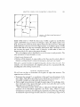
The adaptive grid data structure (in 2-D) is based on a single level uniform grid
superimposed on the data. For example, suppose that we are given N small
straight line segments or edges scattered within a square of side one. (See Figure
1, where N = 4). The grid has G by G cells (G = 3 in Figure 1), each of side B =
I/G. Let L be a measure describing the edges' length, such as the average. The
data structure consists of a set of ordered pairs of a cell number and an edge
number, i.e.,
{(cell, edge)}
Each pair represents an edge passing through a cell. For Figure 1, we obtain the
following data structure:
{(2,1), (1,1), (4,1), (2,2), (5,2), (4,3), (5,3), (6,3), (8,4)}
This data structure bears a superficial resemblance to several others: unlike
Warnock's hidden line algorithm (see Sutherland 1974), the adaptive grid does
not clip an edge into several pieces if it passes through several cells. In the
example, edge # 1 passes through cells # 2 , 1, and 4, but we merely obtain 3
ordered pairs in the set. Unlike a tree (see Nievergelt 1974), or k-d tree (see
Bentley 1975a, andWillard), it divides the data coordinate space evenly indepen-
ADAPTIVE GRIDS FOR GEOMETRIC OPERATIONS
161
FIGURE 1. An adaptive grid superimposed
on four edges.
dently of the order in which the data occur. Unlike a quad tree (see Bentley
1975b, and Finkel 1974) or octree (see Meagher 1982), the adaptive grid is one
level, and does not subdivide in the regions where the data are denser. Although
such a hierarchy is the most obvious 'improvement' to an adaptive grid, it will be
shown later that if the data are reasonably distributed, then a hierarchy would
not increase the speed. Further, such a hierarchy would make it harder to
determine which cells a given edge passes through.
When the adaptive grid is described as a set, the term is used precisely. The
only operations to be performed on it are:
1 Insert a new element, and
1 Retrieve all the elements in some order so that they may be sorted, adjacent
elements combined under certain circumstances, and a new set created.
This gives a great freedom in implementing this abstract data structure. For
example, on a microcomputer, the adaptive grid can be a sequential disk file,
assuming that a file sorting routine exists.
FINDING
INTERSECTIONS
We will now see how to determine all the pairs of edges that intersect. The
operations are as follows:
1 Determine the optimal G, or resolution of the grid, from the statistics of the
input edges. This will be described in more detail later, but letting G = I/L, is
reasonable. Initialize an empty grid data structure for this G.
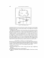
2 Make a single sequential pass through the input edges. For each edge, determine which grid cells it passes through, and for each such cell, insert a (cell,
edge) pair into the grid data structure.
Since determining exactly which cells an edge passes through requires an
extension of the Bresenham algorithm (see Foley 1982), which is a little
complicated, in practice, an enclosing box is placed around the edge. The edge
is considered to pass through all cells in this box. Considering an edge to be in
162
WM
RANDOLPH
FRANKLIN
some extra cells speeds up this section and slows down the pair by pair
comparison in section 5 below.
3 Retrieve the (cell, edge) pairs and sort them by cell number.
4 Make a sequential pass through the sorted list. For each cell mentioned in the
list, determine all the edges that pass through that cell, and combine them into
a set. Now we have a new set:
{(cell, {edge, edge, ...})}
with one element for each cell that has at least one edge passing through it.
Each element has the cell number and a smaller set of the edges that pass
through that cell. Continuing the example of Figure 1, we have at this stage:
{(1,{1} ),
(2, {1,2}),
(4, {1>3}),
(6, {3} ),
(8, {4} )}
Note that since cells 3, 7, and 9 have no edges passing through them, they do
not appear at all here. An empty cell does not use even one word of storage.
5 For each element of this set, i.e., for each cell with at least one edge passing
through it, test all the edges in the cell pair by pair to determine which
intersect. Since two edges that intersect must do so in some cell, and so must
appear together in that cell, this will find all intersections. In the example,
edges 1 and 3 both pass through cell 4, but an exact test shows that they do not
intersect. On the other hand, cell 5 contains edges 2 and 3, and they do
intersect.
6 If a pair of edges that do intersect appear together in more than one cell, then
that intersection will be reported for each such cell. To avoid this duplication,
when an intersection is found, it can be ignored unless it falls in the current
cell. For this strategy to work, the cells must partition the space exactly, i.e.,
each point must fall in exactly one cell. This can be satisfied by considering
each vertical grid line between two cells to be inside its right neighbor, and
considering each horizontal grid line between two grid cells to be inside its
upper neighbor.
TIMING
This method is useful only because it executes efficiently. We will now analyze
the time and determine the optimal G.
Let U = the average number of cells that each edge falls in. Then, approximately
U= 1 + 2LG
However, assuming that we place a box around the edge and count all cells in
that, as described above, we will get a higher figure:
since BG = 1
ADAPTIVE
GRIDS FOR G E O M E T R I C
OPERATIONS
163
We will use this higher number since it is more conservative and does not affect
the rate of growth of the final time. Next, V = total number of (cell, edge) pairs
= NU
= 7V(i + LG)2
Then, W = the average number of edges in each cell
= VVG2
= N(B + L)2
For the execution times, we will use the notation θ(x), which means proportional
to x, as x increases.
Let Ti = the time to calculate the (cell, edge) pairs
= θ(V)
and T2= the time to determine the intersections
= e(G 2 w 2 )
since in each cell, each edge must be tested against each other edge.
So T = total time
= T 1 + T2
= θ(N(1 + LG) + NZG2(B + L)4)
Now, if we let B = 6(L), i.e., the grid size is proportional to the edge length, we
get
T=Q(N+
S)
where
S = N2L2/4
since with 6 notation, which considers only the rate of growth, constant multi­
pliers can be added freely. But S is approximately the expected number of edge
intesections for a given N and L. Since a routine that finds all edge intersections
must examine each edge and each intersection at least once, setting B = cL, for
any c, gives an optimal time, up to a constant factor. The actual c which
minimizes T should be determined heuristically, since it depends on the relative
speeds of various parts of the program, and this may depend on the model of the
computer.
We sometimes have even more freedom to select B, that is, there may be a
range of functions for B that give the same minimum time, depending on the
dependency of L on N as the problems get bigger. We can use this extra freedom
to also minimize space if we wish.
It might be objected that the execution time for any cell depends on the average
of the square of the number of edges in that cell, whereas we have used the square
of the average. However, if the edges are independently and identically distri­
buted, then each edge has the same independent probability of passing through
any given cell. Thus the number of edges in a given cell is Poisson distributed, so
the square of the mean equals the mean of the square.
WM
164
RANDOLPH FRANKLIN
IMPLEMENTATION
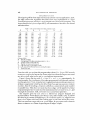
The adaptive grid has been implemented and tested in various applications. First,
the edge intersection algorithm described above was implemented as a Flecs
Fortran preprocessor (see Beyer 1975) program on a Prime midi-computer. The
largest example had 50,000 edges and 47,222 intersections. See table I for a list
of
execution times.
N
Table 1 EXECUTION TIMES FOR EDGE INTERSECTIONS
L
B
S
T1
T2
.100
.100
.010
'5
M3
1000
.100
.100
.010
1000
.030
.030
163
1000
3000
.030
3000
.100
.003
.010
.030
.001
.003
.010
.001
.003
.010
.100
.010
.030
.100
.010
.010
.030
.010
.010
.010
.010
.010
.010
1720
3000
.100
.010
100
300
10000
10000
100000
30000
30000
30000
50000
50000
50000
11
149
1487
15656
156
1813
16633
149
'797
16859
315
4953
47222
.17
•54
'•73
1.72
1.71
5.24
5.41
5-'9
16.36
17.38
17.68
48.33
48.46
52.85
77-71
79.49
86.23
.26
•93
3.62
2.54
4.46
8.05
8.82
27-93
16.45
26.02
44.78
43-95
54.21
98.93
75-75
92.37
278.49
T
.43
1.47
5-35
4.25
6.18
13.29
14.22
33.12
32.82
43.40
67-45
92.28
102.66
151.78
153.46
171.87
364.72
Column Labels
N
Number of edges
L
Average length of edges, assuming screen is 1 by 1
B
Length of side of each grid cell
S
Number of intersections found
T1 CPU time (sec.) to put edges in cells
T2 CPU time to find the intersections among the edges
T
Total CPU time
From the table, we see that this program takes about (N + S)/300 CPU seconds
to execute, even for the largest case. Some other facts about the largest case tested
are: 98,753 (cell, edge) pairs, and 11,534 duplicate intersections.
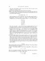
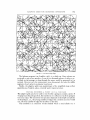
Figure 2 shows the case with N = 1000, G = 10, L = o. 1 approximately. In
these examples, the coordinates of the edges are generated with a pseudo-random
number generator. Now, manufacturer supplied random number generators are
all linear congruential which has the effect that if you pair up successive random
numbers, then the resulting 2-D points will fall on a comparatively small number
of parallel lines. This does not mean that these edges will be parallel if a linear
congruential generator is used since the random numbers are used for x1, y 1, and
the angle of inclination. Still, it is better to use a non-linear generator.
The adaptive grid was next used in a haloed line program designed and
implemented by Varol Akman (see Akman 1981, and Franklin 1980). A haloed
line drawing is a means of displaying a 3-D wire frame model (i.e., edges but not
faces) of an object with front lines cutting gaps in read lines where they cross.
This was tested on scenes with over 10,000 edges. It can process such a scene in
about 10 minutes on a Prime, depending on the edges' lengths.
ADAPTIVE GRIDS FOR G E O M E T R I C O P E R A T I O N S
165
FIGURE 2. 1000 intersecting edges.
The Spheres program (see Franklin 1981), is a third test. Here spheres are
projected on top of one another. A case of ten thousand spheres of radius 0.02,
overlaid on the average 10 deep through the scene, could be processed in 6.4
seconds. Here not only the intersections were determined, but also the visible
segments of each sphere's perimeter were found.
Finally, the adaptive grid is an essential part of the simplified map overlay
algorithm (see Franklin 1983), currently under implementation.
TESTING
WHETHER
A P O I N T IS IN A
POLYGON
The adaptive grid can also be used to test whether a polygon contains a point. If
we preprocess the polygon first, this method is very efficient even if the polygon
has many edges. The execution time per point depends on the depth complexity
of the polygon, i.e., the average number of edges that a random scan line would
cut. The total number of edges has no effect on the time.
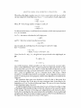
This method is an extension of the method where a semi-infinite ray is
l66
TO
RANDOLPH FRANKLIN
FIGURE 3. Point inpolygon
testing.
extended from the point in some direction to infinity. The point is in the polygon
if and only if the ray cuts an odd number of edges. The problem lies in testing the
ray against every edge.
To speed this up, we will use a one-dimensional version of the adaptive grid on
a line. The line is divided into i-D grid cells and then the polygon's edges are
projected onto the line. Now we know which edges fall into each cell. For
example, see Figure 3, where a polygon with N = 13 edges is projected onto a
i-D grid with G ~ 4 cells. After all the edges in each cell are collected, we know,
for example, that cell # 2 has edges # 2 , 3, 9, and 10. Now, consider point P:
since it also projects into cell # 2 , a ray running vertically up from it can only
intersect those 4 edges, so we need only test it against them. The execution time is
the average number of edges per cell. As the cell size becomes smaller than the
edge size, this number has the polygon's depth complexity as a lower bound.
LOCATING
A POINT
IN A P L A N A R
GRAPH
The obvious extension of the above problem is to take a planar graph and a point,
P, and to determine which polygon of the graph contains P. This can be done by
testing P in turn against each polygon in turn, unless one polygon completely
contains another, but that is slow. A more efficient method is this:
1 Extend a ray up from P.
2 Record all the edges that it crosses, along with those edges' neighboring
polygons.
3 Sort those edges by their ray crossings from P.
4 Finally, P is contained in the lower polygonal neighbor of the closest crossing
edge to P.
ADAPTIVE GRIDS FOR G E O M E T R I C O P E R A T I O N S
167
As before, we put the planar graph's edges into a 1-D adaptive grid and test the
ray against only those edges in the same cell as P's projection.
SUMMARY
Techniques from computational geometry have been shown, both by theoretical
analysis and by implementation, to lead to more efficient means of solving
certain common operations in automated cartography.
ACKNOWLEDGEMENT
This material is based upon work supported by the National Science Foundation
under Grant No. ECS 80-21504.
REFERENCES
AHO, A.v., J.E. HOPCROFT, and J.D. ULLMAN. 1974. The design and analysis of computer algorithms,
Addison-Wesley, Reading, Mass.
AKMAN, V. 1981. HALO - A computer graphics program for efficiently obtaining the haloed line
drawings of computer aided design models of wire-frame objects, User's manual and Program
logic manual, Rensselaer Polytechnic Institute, Image Processing Lab.
BENTLEY, J.L. 1975a. Multidimensional binary search trees used for associative searching, Comm.
ACM 18(9), pp. 509- 517.
BENTLEY, J.L. and D.F. STAN AT. 1975b. Analysis of range searches in quad trees, Information
Processing Letters, 3(6), pp. 170-173.
BENTLEY, J.L. and T.A. OTTMANN. 1979. Algorithms for reporting and counting geometric intersections, IEEE Trans, on Computers, C-28(9), PP- 643—647.
BENTLEY, J.L. and D. WOOD. 1980. An optimal worst case algorithm for reporting intersections of
rectangles, IEEE Trans, on Computers, 0-29(7), pp. 571-576.
BEYER, T. 1975. Flees: User's manual, Dept. of Computer Science, University of Oregon.
DOBKIN, D. and R.J. LIPTON. 1976. Multidimensional searching problems, SIAM J. Comput., 5(2),
pp. 181-186.
FINKEL, R.A. and J.L. BENTLEY. 1974. Quadtrees: a data structure for retrieval on composite key, Acta
Inform., 4, pp. 1-9.
FOLEY, J.D. and A. VAN DAM. 1982. Fundamentals of interactive computer graphics, Addison-Wesley,
Reading, Mass.
FRANKLIN, w.R. 1980. Efficiently computing the haloed line effect for hidden-line
elimination,
Rensselaer Polytechnic Institute, Image Processing Lab, IPL-81-004.
1981. An exact hidden sphere algorithm that operates in linear time, Computer Graphics and
Image Processing, 15, pp. 364-379.
1983. A simplified map overlay algorithm, presented at Harvard Computer Graphics Conference, Cambridge, Mass., August 1983.
MEAGHER, D.j. 1982. The octree encoding method for efficient solid modelling, Ph.D. thesis,
Rensselaer Polytechnic Institute.
NIEVERGELT, J. 1974. Binary search trees and file organization, A CM Computing Surveys, 6(3), pp.
195-207.
PEUCKER, T.K., and N. CHRISMAN. 1975. Cartographic data structures, The American Cartographer,
2(1), pp. 55-69.
SUTHERLAND, I.E., R.F. SPROULL, and R.A. scHUMACKER. 1974. A characterization of ten hidden
surface algorithms, Computing Surveys, 6(1), pp. 1-55.
WILLARD, D.E. Informative abstract: new data structures for orthogonal queries, Harvard University.