1
Programming Methodologies in GCLA*
Göran Falkman & Olof Torgersson
Department of Computing Science, Chalmers University of Technology
S-412 96 Göteborg, Sweden
{falkman,oloft}@cs.chalmers.se
Abstract. This paper presents work on programming methodologies for the programming tool GCLA. Three methods are discussed which show how to construct the control part of a GCLA program, where the definition of a specific
problem and the set of intended queries are given beforehand. The methods are
described by a series of examples, but we also try to give a more explicit description of each method. We also discuss some important characteristics of the methods.
1 Introduction
This paper contributes to the as yet poorly known domain of programming methodology for the programming tool GCLA.
A GCLA program consists of two separate parts; a declarative part and a control
part. When writing GCLA programs we therefore have to answer the question: “Given
a definition of a specific problem and a set of queries, how can we construct the control
knowledge that is required for the resulting program to have the intended behavior?” Of
course there is no definite answer to this question, new problems may always require
specialized control knowledge, depending on the complexity of the problem at hand, the
complexity of the intended queries etc. If the programs are relatively small and simple
it is often the case that the programs can be categorized, as for example functional programs or object-oriented programs, and we can then use for these categories rather standard control knowledge. But if the programs are large and more complex such a
classification is often not possible since most large and complex programs are mixtures
of functions, predicates, object-oriented techniques etc., and therefore the usage of
more general control knowledge is often not possible. Thus, there is a need for more
systematic methods for constructing the control parts of large and complex programs.
In this paper we discuss three different methods of constructing the control part of
GCLA programs, where the definitions and the sets of intended queries are given
beforehand. The work is based on our collective experiences from developing large
GCLA applications.
The rest of this paper is organized as follows. In Sect. 2 we give a very short intro*.
This work was carried out as part of the work in the ESPRIT working group GENTZEN and
was funded by The Swedish National Board for Industrial and Technical Development
(NUTEK).
duction to GCLA. In Sect. 3 we present three different methods for constructing the
control part of a GCLA program. The methods are described by a series of examples,
but we also try to give a more explicit description of each method. In Sect. 4 we present
a larger example of how to use each method in practice. Since we are mostly interested
in large and more complex programs we want the methods to have properties suitable
for developing such programs. In Sect. 5 we therefore evaluate each method according
to five criteria on how good we perceive the resulting programs to be. In Sect. 6 finally,
we summarize the discussion in Sect. 5, and we also make some conclusions about possible future extensions of the GCLA system.
2 Introduction to GCLA
The programming system Generalized Horn Clause LAnguage (GCLA1) [1, 3, 4, 5] is
a logical programming language (specification tool) that is based on a generalization of
Prolog. This generalization is unusual in that it takes a quite different view of the meaning of a logic program — a definitional view rather than the traditional logic view.
Compared to Prolog, what has been added to GCLA is the possibility of assuming
conditions. For example, the clause
a <= (b -> c).
should be read as: “a holds if c can be proved while assuming b.”
There is also a richer set of queries in GCLA than in Prolog. In GCLA, a query corresponding to an ordinary Prolog query is written
\- a.
and should be read as: “Does a hold (in the definition D)?” We can also assume things
in the query, for example
c \- a.
which should be read as: “Assuming c, does a hold (in the definition D)?”, or “Is a
derivable from c?”
To execute a program, a query G is posed to the system asking whether there is a
substitution σ such that Gσ holds according to the logic defined by the program. The
goal G has the form Γ |− c, where Γ is a list of assumptions, and c is the conclusion from
the assumptions Γ. The system tries to construct a deduction showing that Gσ holds in
the given logic.
GCLA is also general enough to incorporate functional programming as a special
case.
For a more complete and comprehensive introduction to GCLA and its theoretical
properties see [5]. [1] contains some earlier work on programming methodologies in
GCLA. Various implementation techniques, including functional and object-oriented
programming, are also demonstrated. For an introduction to the GCLA system see [2].
1.
To be pronounced “gisela”.
2.1
GCLA Programs
A GCLA program consists of two parts; one part is used to express the declarative content of the program, called the definition or the object level, and the other part is used to
express rules and strategies acting on the declarative part, called the rule definition or
the meta level.
The Definition. The definition constitutes the formalization of a specific problem
domain and in general contains a minimum of control information. The intention is that
the definition by itself gives a purely declarative description of the problem domain
while a procedural interpretation of the definition is obtained only by putting it in the
context of the rule definition.
The Rule Definition. The rule definition contains the procedural knowledge of the
domain, that is the knowledge used for drawing conclusions based on the declarative
knowledge in the definition. This procedural knowledge defines the possible inferences
made from the declarative knowledge.
The rule definition contains inference rule definitions which define how different
inference rules should act, and search strategies which control the search among the
inference rules.
The general form of an inference rule is
Rulename(A1,…,Am,PT1,…,PTn) <=
Proviso,
(PT1 -> Seq1),
…,
(PTn -> Seqn)
-> Seq.
and the general forms of a strategy are
Strat(A1,…,Am) <= PT1,…,PTn.
or
Strat(A1,…,Am) <=
(Proviso1 -> Seq1),
…,
(Provisok -> Seqk).
Strat(A1,…,Am) <= PT1,…,PTn.
where
• Ai are arbitrary arguments.
• Proviso is a conjunction of provisos, that is calls to Horn clauses defined elsewhere. The Proviso could be empty.
• Seq and Seqi are sequents which are on the form (Antecedent \Consequent), where Antecedent is a list of terms and Consequent is an ordinary GCLA term.
• PTi are proofterms, that is terms representing the proofs of the premises, Seqi.
Example: Default Reasoning. Assume we know that an object can fly if it is a bird
and if it is not a penguin. We also know that Tweety and Polly are birds as well as are
all penguins, and finally we know that Pengo is a penguin. This knowledge is expressed
in the following definition:
flies(X) <=
bird(X),
(penguin(X) -> false).
bird(tweety).
bird(polly).
bird(X) <= penguin(X).
penguin(pengo).
One possible rule definition enabling us to use this definition the way we want, is:
fs <=
right(fs),
left_if_false(fs).
% First try standard right rules,
% else if consequent is false.
left_if_false(PT) <=
(_ \- false).
left_if_false(PT) <=
no_false_assump(PT),
false_left(_).
% Is the consequent false?
no_false_assump(PT) <=
not(member(false,A))
-> (A \- _).
no_false_assump(PT) <=
left(PT).
% No false assumption,
% that is the term false is not a
% member of the assumption list.
member(X,[X|_]).
member(X,[_|R]):member(X,R).
% Proviso definition.
% If so perform left rules.
If we want to know which birds can fly, we pose the query
fs \\- (\- flies(X)).
and the system will respond with X = tweety and X = polly.
If we want to know which birds cannot fly, we can pose the query
fs \\- (flies(X) \- false).
and the system will respond with X = pengo.
3 How to Construct the Procedural Part
3.1
Example: Disease Expert System
Suppose we want to construct a small expert system for diagnosing diseases. The following definition defines which symptoms are caused by which diseases:
symptom(high_temp) <= disease(pneumonia).
symptom(high_temp) <= disease(plague).
symptom(cough) <= disease(pneumonia).
symptom(cough) <= disease(cold).
In this application the facts are submitted by the queries. For example, if we want to
know which diseases cause the symptom high temperature we can pose the query:
disease(X) \- symptom(high_temp).
Another possible query is
disease(X) \- (symptom(high_temp),symptom(cough)).
which should be read as: “Which diseases cause high temperature and coughing?” If we
want to know which possible diseases follow, assuming the symptom high temperature,
we can pose the query:
symptom(high_temp) \- (disease(X);disease(Y)).
Yet another query is
disease(pneumonia) \- symptom(X).
which should be read as: “Which symptoms are caused by the disease pneumonia?”
We will in the following three subsections use the definition and the queries above,
to illustrate three different methods of constructing the procedural part of a GCLA program.
3.2
Method 1: Minimal Stepwise Refinement
The general form of a GCLA query is S ||− Q where S is a proofterm, that is some more
or less instantiated inference rule or strategy, and Q is an object level sequent. One way
of reading this query is: “S includes a proof of Qσ for some substitution σ.”
When the GCLA system is started the user is provided with a basic set of inference
rules and some standard strategies implementing common search behavior among these
rules. The standard rules and strategies are very general, that is they are potentially useful for a large number of definitions, and provide the possibility of posing a wide variety
of queries.
We show some of the standard inference rules and strategies here, the rest can be
found in [2].
One simple inference rule is axiom/3 which states that anything holds if it is
assumed. The standard axiom/3 rule is applicable to any terms and is defined by:
axiom(T,C,I) <=
term(T),
term(C),
unify(T,C)
->(I@[T|R] \- C).
%
%
%
%
proviso
proviso
proviso
conclusion
The proof of a query is built backwards, starting from the goal sequent. So, in the rule
above we are trying to prove the last line, that is the conclusion of the rule. Note that
when an inference rule is applied, the conclusion is unified with the sequent we are trying to prove before the provisos and the premises of the rule are tried. Thus, the axiom/
3 rule tells us that if we have an assumption T among the list of assumptions I@[T|R]
(where ‘@’/2 is an infix append operator) and if both T and the conclusion C are terms,
and if T and C are unifiable, then C holds.
Another standard rule is the definition right rule, d_right/2. The conclusions that
can be made from this rule depend on the particular definition at hand. The d_right/
2 rule applies to all atoms:
d_right(C,PT) <=
atom(C),
clause(C,B),
(PT -> (A \- B))
-> (A \- C).
%
%
%
%
C must be an atom
proviso
premise, use PT to prove it
conclusion
This rule could be read as: “If we have a sequent A \- C, and if there is a clause
D <= B in the definition, such that C and D are unifiable by a substitution σ, and if we
can show that the sequent A \- B holds using some of the proofs represented by the
proofterm PT, then (A \- C)σ holds by the corresponding proof in d_right(C,PT).
There is also an inference rule, definition left, which uses the definition to the left.
This rule, d_left/3, is applicable to all atoms:
d_left(T,I,PT) <=
atom(T),
%
definiens(T,Dp,N),
%
(PT -> (I@[Dp|Y] \- C)) %
-> (I@[T|Y] \- C).
%
T must be an atom
Dp is the definiens of T
premise, use PT to prove it
conclusion.
The definiens operation is described in [5]. If T is not defined Dp is bound to false.
As an example of an inference rule that applies to a constructed condition we show
the a_right/2 rule which applies to any condition constructed with the arrow constructor ‘->’/2 occurring to the right of the turnstile, ‘\-’:
a_right((A -> C),PT) <=
(PT -> ([A|P] \- C))
-> (P \- (A -> C)).
% premise, use PT to prove it
% conclusion
One very general search strategy among the predefined inference rules is arl/0, which
in each step of the derivation first tries the axiom/3 rule, then all standard rules operating on the consequent of a sequent and after that all standard rules operating on elements of the antecedent. It is defined by:
arl <=
axiom(_,_,_),
right(arl),
left(arl).
% first try the rule axiom/3,
% then try strategy right/1,
% then try strategy left/1.
Another very general search strategy is lra/0:
lra <=
left(lra),
right(lra),
axiom(_,_,_).
% first try the strategy left/1,
% then try strategy right/1,
% then try rule axiom/3.
If we are not interested in the antecedent of sequents, we can use the standard strategy
r/0, with the definition:
r <= right(r).
In the definitions below of the strategies right/1 and left/1, user_add_right/2
and user_add_left/3 can be defined by the user to contain any new inference rules
or strategies desired:
right(PT) <=
user_add_right(_,PT),
v_right(_,PT,PT),
a_right(_,PT),
o_right(_,_,PT),
true_right,
d_right(_,PT).
% try users specific rules first
% then standard right rules
left(PT) <=
user_add_left(_,_,PT), % try users specific rules first
false_left(_),
% then try standard left rules
v_left(_,_,PT),
a_left(_,_,PT,PT),
o_left(_,_,PT,PT),
d_left(_,_,PT),
pi_left(_,_,PT).
We see that all these default rules and strategies are very general in the sense that they
contain no domain specific information, apart from the link to the definition provided
by the provisos clause/2 and definiens/3, and also in the sense that they span a
very large proof search space.
Constructing the Procedural Part. Now, the idea in the minimal stepwise refinement method, is that given a definition D and a set of intended queries Q, we do as little
as possible to construct the procedural part P, that is we try to find strategies S1, …, Sn
among the general strategies given by the system, such that Si ||− Qi, with the intended
procedural behavior for each of the intended queries. If such strategies exist then we are
finished, and constructing the procedural part was trivial indeed. In most cases however
there will be some queries for which we cannot find a predefined strategy which
behaves correctly, they all give redundant answers or wrong answers or even no
answers at all.
When there is no default strategy which gives the desired procedural behavior, we
choose the predefined strategy that seems most appropriate and try to alter the set of
proofs it represents so that it will give the desired procedural behavior. To do this we
use the tracer and the statistical package of the GCLA system to localize the point in the
search space of a proof of the query which causes the faulty behavior. Once we have
found the reason behind the faulty behavior we can remove the error by changing the
definition of the procedural part. We then try all our queries again and repeat the procedure of searching for and correcting errors of the procedural part until we achieve
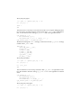
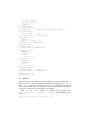
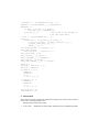
proper procedural behavior for all the intended queries. The method is illustrated in
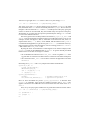
Fig. 1.
G
H
E
F
C
B
D
A
Fig. 1. Proof search space for a query S ||− A. A is the query we pose to the
system. The desired procedural behavior is the path leading to G marked in the
figure, however the strategy S instead takes the path via F to H. We localize the
choice-point to C and change the procedural part so that the edge C—E is chosen
instead.
Example: Disease Expert System Revisited. We try to use the disease program
with some standard strategies. For example, in the query below, the correct answers are
X = pneumonia and, on backtracking, X = plague. The true answers mean that
there exists a proof of the query, but it gives no binding of the variable X.
First we try the strategy arl/0:
| ?- arl \\- (disease(X) \- symptom(high_temp)).
X = pneumonia ? ;
true ? ;
true ? ;
true ? ;
X = plague ? ;
After this we get eight more true answers. Then we try the strategy lra/0:
| ?- lra \\- (disease(X) \- symptom(high_temp)).
This query gives eight true answers before giving the answer pneumonia the ninth
time, then three more true answers and finally the answer plague. We see that even
though it is the case that both arl/0 and lra/0 include proofs of the query giving the
answers in which we are interested, they also include many more proofs of the query.
We therefore try to restrict the set of proofs represented by the strategy arl/0 in order
to remove the undesired answers.
The most typical sources of faulty behavior are that the d_right/2, d_left/3 and
axiom/3 rules are applicable in situations where we would rather see they were not. An
example of what can happen is that if, somewhere in the derivation tree, there is a
sequent of the form p \- X, where p is not defined, and the inference rule d_left/3
is tried and found applicable, we get the new goal false \- X, which holds since anything can be shown from a false assumption, if we use a strategy such as arl/0 or lra/
0 that contains the false_left/1 rule.
By using the tracer we find that this is what happens in our disease example, where
d_left/3 is tried on the undefined atom disease/1. To get the desired procedural
behavior there are at least two things we could do:
• We could delete the inference rule false_left/1 from our global arl/0 strategy, but then we would never be able to draw a conclusion from a false assumption.
• We could restrict the d_left/3 rule so that it would not be applicable to the atom
disease/1.
Restricting the d_left/3 rule is very simple and could be made like this:
d_left(T,I,PT) <=
d_left_applicable(T),
definiens(T,Dp,N),
(PT -> (I@[Dp|R] \- C))
-> (I@[T|R] \- C).
d_left_applicable(T):atom(T),
not(functor(T,disease,1)).
% standard restriction on T
% application specific.
Here we have introduced the proviso d_left_applicable/1 to describe when
d_left/3 is applicable. Apart from the standard restriction that d_left/3 only
applies to atoms we have added the extra restriction that the atom must not be disease/1.
Now, we try our query again, and this time we get the desired answers and no others:
| ?- arl \\- (disease(X) \- symptom(high_temp)).
X = pneumonia ? ;
X = plague ? ;
no
With this restriction on the d_left/3 rule the arl/0 strategy correctly handles all the
queries in Sect. 3.1.
Further Refining. One very simple optimization is to use the statistical package of
GCLA and remove any inference rules that are never used from the procedural part.
Sometimes there is a need to introduce new inference rules, for example to handle
numbers in an efficient way. We can then associate an inference rule with each operation
and use this directly to show that something holds. Such new inference rules could then
be placed in one of the strategies user_add_right/2 or user_add_left/2 which
are part of the standard strategies right/1 and left/1.
3.3
Method 2: Splitting the Condition Universe
With the method in the previous section we started to build the procedural part without
paying any particular attention to what the definition and the set of intended queries
looked like. If we study the structure of the definition, and of the data handled by the
program, it is possible to use the knowledge we gain to be able to construct the procedural part in a more well-structured and goal-oriented way.
The basic idea in this section is that given a definition D and a set of intended queries
Q, it is possible to divide the universe of all object-level conditions into a number of
classes, where every member of each class is treated uniformly by the procedural part.
Examples of such classes could be the set of all defined atoms, the set of all terms which
could be evaluated further, the set of all canonical terms, the set of all object level variables etc.
In order to construct the procedural part of a given definition, we first identify the
different classes of conditions used in the definition and in the queries, and then go on
to write the rule definition in such a way that each rule or strategy becomes applicable
to the correct class or classes of conditions. The resulting rule definition typically consists of some subset of the predefined inference rules and strategies, extended with a
number of provisos which identify the different classes and decide the applicability of
each rule or strategy.
Of course the described method can only be used if it is possible to divide the objectlevel condition universe in some suitable set of classes; for some applications this will
be very difficult or even impossible to do.
3.4
A Typical Split
The most typical split of the universe of object-level conditions is into one set to which
the d_right/2 and d_left/3 rules but not the axiom/3 rule apply, and another set
to which the axiom/3 rule but not the d_right/2 or d_left/3 rules apply. To handle
this, and many other similar situations easily, we change the definition of these rules:
d_right(C,PT) <=
d_right_applicable(C),
clause(C,B),
(PT -> (A \- B))
-> (A \- C).
d_left(T,I,PT) <=
d_left_applicable(T),
definiens(T,Dp,N),
(PT -> (I@[Dp|R] \- C))
-> (I@[T|R] \- C).
axiom(T,C,I) <=
axiom_applicable(T),
axiom_applicable(C),
unify(C,T)
-> (I@[T|_] \- C).
All we have to do now is alter the provisos used in the rules above according to our split
of the universe to get different procedural behaviors. With the proviso definitions
d_right_applicable(C) :- atom(C).
d_left_applicable(T) :- atom(T).
axiom_applicable(T) :- term(T).
we get exactly the same behavior as with the predefined rules.
Example 1: The Disease Example Revisited. The disease example is an example
of an application where we can use the typical split described above. We know that the
d_right/2 and the d_left/3 rules should only be applicable to the atom symptom/
1, so we define the provisos d_right_applicable/1 and d_left_applicable/1
by:
d_right_applicable(C) :- functor(C,symptom,1).
d_left_applicable(T) :- functor(T,symptom,1).
We also know that the axiom/3 rule should only be applicable to the atom disease/
1, so axiom_applicable/1 thus becomes:
axiom_applicable(T) :- functor(T,disease,1).
Example 2: Functional Programming. One often occurring situation, for example
in functional programming, is that we can split the universe of all object level terms into
the two classes of all fully evaluated expressions and variables and all other terms
respectively.
For example, if the class of fully evaluated expressions consists of all numbers and
all lists, it can be defined with the proviso canon/1:
canon(X) :- number(X).
canon([]).
canon(X) :- functor(X,’.’,2).
To get the desired procedural behavior we restrict the axiom/3 rule to operate on the
class defined by the above proviso and the set of all variables, and the d_right/2 and
d_left/3 rules to operate on any other terms, thus:
d_right_applicable(T):atom(T),not(canon(T)). % noncanonical atom
d_left_applicable(T):atom(T),not(canon(T)). % noncanonical atom
axiom_applicable(T) :- var(T).
axiom_applicable(T) :- nonvar(T),canon(T).
Here we use not/1 to indicate that if we cannot prove that a term belongs to the class
of canonical terms then it belongs to the class of all other terms.
3.5
Method 3: Local Strategies
Both of the previous methods are somehow based on the idea that we should start with
a general search strategy, among the inference rules at hand, and restrict or augment the
set of proofs it represents in order to get the desired procedural behavior from a given
definition and its associated set of intended queries. However, we could just as well do
it the other way around and study the definition and the set of intended queries and construct a procedural part, that gives us exactly the procedural interpretation we want right
from the start, instead of performing a tedious procedure of repeatedly cutting away (or
adding) branches of the proof search space of some general strategy. In this section we
will show how this can easily be done for many applications. Any examples will use the
standard rules, but the method as such works equivalently with any set of rules.
Collecting Knowledge. When constructing the procedural part we try to collect and
use as much knowledge as possible about the definition, the set of intended queries, of
how the GCLA system works etc. Among the things we need to take into account in
order to construct the procedural part properly are:
• We need to have a good idea of how the GCLA system tries to construct the proof
of a query.
• We must have a thorough understanding of the interpretation of the predefined
rules and strategies, and of any new rules or strategies we write.
• We must decide exactly what the set of intended queries is. For example, in the disease example this set is as described in Sect. 3.1.
• We must study the structure of the definition in order to find out how each defined
atom should be used procedurally in the queries. This involves among other things
considering whether it will be used with the d_left/3 or the d_right/2 rule or
both. For example, in the disease example we know that both the d_left/3 and
the d_right/2 rule should be applicable to the atom symptom/1, but that neither
of them should be applicable to the atom disease/1. We also use knowledge of
the structure of the possible sequents occurring in a derivation, to decide if we will
need a mechanism for searching among several assumptions or to decide where to
use the axiom/3 rule etc. For example, in the disease example we know that the
axiom/3 rule should be applicable to the atom disease/1, but not to the atom
symptom/1.
Constructing the Procedural Part. Assume that we have a set of condition constructors, C, with a corresponding set of inference rules, R. Given a definition D which
defines a set of atoms DA, a set of intended queries Q and possibly another set UA of
undefined atoms which can occur as assumptions in a sequent, we do the following to
construct strategies for each element in the set of intended queries:
•
Associate with each atom in the sets DA and UA, a distinct procedural part that
assures that the atoms are used the way we want in all situations where they can
occur in a derivation tree. The procedural part associated with an atom is built using
the elements of R, d_right/2, d_left/3, axiom/3, strategies associated with
other atoms and any new inference rules needed.
We can then use the strategies defined above to build higher-level strategies for all the
intended queries in Q.
For example, in the disease example C is the set {‘;’/2,‘,’/2}, R is the set
{o_right/3,o_left/4,v_right/3,v_left/3}, D and Q are as given in Sect. 3.1,
DA is the set {symptom/1} and UA is the set {disease/1}.
According to the method we should first write distinct strategies for each member
of DA, that is symptom/1. The atom symptom/1 can occur on the right side of the
object level sequent so we write a strategy for this case:
symptom_r <= d_right(symptom(_),disease).
When symptom/1 occurs on the right side we want to look up the definition of symptom/1 so we use the d_right/2 rule, giving a new object level sequent of the form
A \- disease(X), and we therefore continue with the strategy disease/0.
Now, symptom/1 is also used on the left side and since we can not use symptom_r/
0 to the left, we have to introduce a new strategy for this case, symptom_l/0:
symptom_l <= d_left(symptom(_),_,symptom_l2).
symptom_l2 <=
o_left(_,_,symptom_l2,symptom_l2),
o_right(_,_,symptom_l2),
disease.
When symptom/1 occurs on the left side we want to calculate the definiens of symptom/1 so we can use the d_left/3 rule, giving a new object level sequent of the form
(disease(Y1);…;disease(Yn)) \- (disease(X1);…;disease(Xk)). In this
case we continue with the strategy symptom_l2/0, which handles sequents of this
form. The strategy symptom_l2/0 uses the strategy disease/0 to handle the individual disease/1 atoms.
We now define the disease/0 strategy:
disease <= axiom(disease(_),_,_).
Finally we use the strategies defined above to construct strategies for all the intended
queries. The first kind of query is of the form disease(D) \symptom(X1),…,symptom(Xn). These queries can be handled by the following
strategy:
d1 <= v_right(_,symptom_r,d1),symptom_r.
The
second
kind
of
query
is
of
the
form
symptom(S) \(disease(X1);…; disease(Xn)). These queries are handled by the strategy d2/0:
d2 <= symptom_l.
What we actually do with this method is to assign a local procedural interpretation to
each atom in the sets DA and UA. This local procedural interpretation is specialized to
handle the particular atom correctly in every sequent in which it occurs. The important
thing is that the procedural part associated with an atom ensures that we will get the correct procedural behavior if we use it in the intended way, no matter what rules or strategies we write to handle other atoms of the definition. Since each atom has its own local
procedural interpretation, we can use different programming methodologies and different sorts of procedural interpretations for the particular atom in different parts of the
program.
In practice this means that for each atom in DA and UA we write one or more strategies which are constructed to correctly handle the particular atom. One way to do this
is to define the basic procedural behavior of each atom, by which we mean that given
an atom, say p/1, we define the basic procedural behavior of p/1 (in this application)
as how we want it to behave in a query where it is directly applicable to one of the inference rules d_right/2, d_left/3 or axiom/3, that is queries of the form A \- p(X)
or A1,…,p(X),…,An \- C.
Since the basic strategy of an atom can use the basic strategy of any other defined
atom if needed, and since strategies of more complex queries can use any combination
of strategies, we will get a hierarchy of strategies, where each member has a welldefined procedural behavior. In the bottom of this hierarchy we find the strategies that
do not use any other strategies, only rules, and in the top we have the strategies used by
a user to pose queries to the system.
Example. In the disease example we constructed the procedural part bottom-up. In
practice it is often better to work top-down from the set of intended queries, since most
of the time we do not know exactly what strategies are needed beforehand.
This means that we start with an intended query, say A1,…,An \- p(X), constructing a top level strategy for this assuming that we already have all sub-strategies we
need, and then go on to construct these sub-strategies so that they behave as we have
assumed them to do.
The following small example could be used to illustrate the methodology:
classify(X) <=
wheels(W),engine(E),(class(wheels(W),engine(E)) -> X).
class(wheels(4),engine(yes)) <= car.
class(wheels(2),engine(yes)) <= motorbike.
class(wheels(2),engine(no)) <= bike.
The only intended query is A1,…,An \- classify(X), where we use the left-hand
side to give observations and try to conclude a class from them, for example:
| ?- classify \\- (engine(yes),wheels(2) \- classify(X)).
X = motorbike ? ;
no
We start from the top and assuming that we have suitable strategies for the queries
A1,…,An \- wheels(X), A1,…,An \engine(X) and A1,…,class(X),…,An \- C, we construct the top level strategy
classify/0:
%classify \\- (A \- classify(X))
classify <=
d_right(_,v_rights(_,_,[wheels,engine,a_right(_,class)])).
where v_rights/3 is a rule that is used as an abbreviation for several consecutive
applications of the v_right/3 rule. All we have left to do now is to construct the substrategies. The strategies engine/0 and wheels/0 are identical; engine/1 and
wheels/1 are given as observations in the left-hand side, so we use the axiom/3 rule
to communicate with the right side, giving the basic strategies:
%engine \\- (A1,…,engine(X),…,An \- Conc)
engine <= axiom(engine(_),_,_).
%wheels \\- (A1,…,wheels(X),…,An \- Conc)
wheels <= axiom(wheels(_),_,_).
Finally class/0 is a function from the observed properties to a class, and the rule definition we want is:
%class \\- (A1,…,class(X,Y),…,An \- Conc)
class <= d_left(class(_,_),I,axiom(_,_,I)).
Of course we do not always have to be so specific when we construct the strategies and
sub-strategies if we find it unnecessary.
4 A Larger Example: Quicksort
In this section we will use the three methods described above to develop some sample
procedural parts to a given definition and an intended set of queries. Of course, due to
lack of space it is not possible to give a realistic example, but we think that the basic
ideas will shine through.
The given definition is a quicksort program, earlier described in [1] and [2], which
contains both functions and relational programming as well as the use of new condition
constructors.
4.1
The Definition
Here is the definition of the quicksort program:
qsort([]) <= [].
qsort([F|R]) <=
pi L \ (pi G \ (split(F,R,L,G) ->
append(qsort(L),cons(F,qsort(G))))).
split(_,[],[],[]).
split(E,[F|R],[F|Z],X) <= E >= F,split(E,R,Z,X).
split(E,[F|R],Z,[F|X]) <= E < F,split(E,R,Z,X).
append([],F) <= F.
append([F|R],X) <= cons(F,append(R,X)).
append(X,Y)#{X \= [_|_],X \= []} <=
pi Z\ ((X -> Z) -> append(Z,Y)).
cons(X,Y) <= pi Z \ (pi W \ ((X -> Z), (Y -> W) -> [Z|W])).
In the definition above qsort/1, append/2 and cons/2 are functions, while split/
4 is a relation. There are also two new condition constructors: ‘>=’/2 and ‘<’/2.
We will only consider one intended query
qsort(X) \- Y.
where X is a list of numbers and Y is a variable to be instantiated to a sorted permutation
of X.
4.2
Method 1
We first try the predefined strategy gcla/0 (the same as arl/0):
| ?- gcla \\- (qsort([4,1,2]) \- X).
X = qsort([4,1,2]) ?
yes
By using the debugging tools, we find out that the fault is that the axiom/3 rule is applicable to qsort/1. We therefore construct a new strategy, q_axiom/3, that is not applicable to qsort/1:
q_axiom(T,C,I) <=
not(functor(T,qsort,1)) -> (I@[T|_] \- C).
q_axiom(T,C,I) <= axiom(T,C,I).
We must also change the arl/0 strategy so that it uses q_axiom/3 instead of axiom/
3:
arl <= q_axiom(_,_,_),right(arl),left(arl).
Then we try the query again:
| ?- gcla \\- (qsort([4,1,2]) \- X).
no
This time the fault is that we have no rules for the new condition constructors ‘>=’/2
and ‘<’/2. So we write two new rules, ge_right/1 and lt_right/1, which we add
to the predefined strategy user_add_right/2:
ge_right(X >= Y) <=
number(X),
number(Y),
X >= Y
-> (A \- X >= Y).
lt_right(X < Y) <=
number(X),
number(Y),
X < Y
-> (A \- X < Y).
Here number/1 is a predefined proviso.
We try the query again:
| ?- gcla \\- (qsort([4,1,2]) \- X).
X = append(qsort([1,2]),cons(4,qsort([]))) ?
yes
We find out that the fault is that the q_axiom/3 strategy should not be applicable to
append/2. We therefore refine the strategy q_axiom/3 so it is not applicable to
append/2 either:
q_axiom(T,C,I) <=
not(functor(T,qsort,1),
not(functor(T,append,2) -> (I@[T|_] \- C).
q_axiom(T,C,I) <= axiom(T,C,I).
We try the query again:
| ?- gcla \\- (qsort([4,1,2]) \- X).
...
This time we get no answer at all. The problem is that the q_axiom/3 strategy is applicable to cons/2. So we refine q_axiom/3 once again:
q_axiom(T,C,I) <=
not(functor(T,qsort,1)),
not(functor(T,append,2)),
not(functor(T,cons,2)) -> (I@[T|_] \- C).
q_axiom(T,C,I) <= axiom(T,C,I).
We try the query again:
| ?- gcla \\- (qsort([4,1,2]) \- X).
X = [1,2,4] ? ;
true ?
yes
The first answer is obviously correct but the second is not. Using the debugging facilities once again, we find out that the problem is that the d_left/3 rule is applicable to
lists, so we construct a new strategy, q_d_left/3, that is not applicable to lists:
q_d_left(T,I,_) <=
not(functor(T,[],0)),
not(functor(T,’.’,2)) -> (I@[T|_] \- _).
q_d_left(T,I,PT) <= d_left(T,I,PT).
We must also change the left/1 strategy, so that it uses the new q_d_left/3 strategy
instead of the d_left/3 rule:
left(PT) <=
user_add_left(_,_,PT),
false_left(_),
v_left(_,_,PT),
a_left(_,_,PT,PT),
o_left(_,_,PT,PT),
q_d_left(_,_,PT),
pi_left(_,_,PT).
We try the query again:
| ?- gcla \\- (qsort([4,1,2]) \- X).
X = [1,2,4] ? ;
X = [1,2,_A] ?
yes
The second answer is still wrong. The fault is that q_d_left/3 is applicable to numbers. We therefore refine the strategy q_d_left/3 so it is not applicable to numbers
either:
q_d_left(T,I,_) <=
not(functor(T,[],0)),
not(functor(T,’.’,2)),
not(number(T)) -> (I@[T|_] \- _).
q_d_left(T,I,PT) <= d_left(T,I,PT).
We try the query once again:
| ?- gcla \\- (qsort([4,1,2]) \- X).
X = [1,2,4] ? ;
no
And finally we get all the correct answers and no others.
One last simple refinement is to use the statistical package to remove unused strategies and rules. The complete rule definition thus becomes:
arl <= q_axiom(_,_,_),right(arl),left(arl).
left(PT) <=
a_left(_,_,PT,PT),
q_d_left(_,_,PT),
pi_left(_,_,PT).
q_d_left(T,I,_) <=
not(functor(T,[],0)),
not(functor(T,’.’,2)),
not(number(T)) -> (I@[T|_] \- _).
q_d_left(T,I,PT) <= d_left(T,I,PT).
user_add_right(C,_) <= ge_right(C),lt_right(C).
q_axiom(T,C,I) <=
not(functor(T,qsort,1)),
not(functor(T,append,2)),
not(functor(T,cons,2)) -> (I@[T|_] \- C).
q_axiom(T,C,I) <= axiom(T,C,I).
ge_right(X >= Y) <=
number(X),
number(Y),
X >= Y
-> (A \- X >= Y).
lt_right(X < Y) <=
number(X),
number(Y),
X < Y
-> (A \- X < Y).
constructor('>=',2).
constructor('<',2).
4.3
Method 2
First we use our knowledge about the general structure of GCLA programs. Among the
default rules all but d_left/3, d_right/2 and axiom/3 are applicable to condition
constructors only. One possible split is therefore the set of all constructors and the set
of all conditions that are not constructors, that is terms:
cond_constr(E) :- functor(E,F,A),constructor(F,A).
terms(E) :- term(E).
Now, all terms can in turn be divided into variables and terms that are not variables, that
is atoms. We therefore split the terms/1 class into the set of variables and the set of
atoms:
vars(E) :- var(E).
atoms(E) :- atom(E).
The atoms can be divided further into all defined atoms and all undefined atoms. In this
application we only want to apply the d_left/3 and d_right/2 rules to defined
atoms. We also know that the only undefined atoms are numbers and lists, that is the
data handled by the program, so one natural split could be the set of all defined atoms
and the set of all undefined atoms:
def_atoms(E) :functor(E,F,A),d_atoms(DA),member(F/A,DA).
undef_atoms(E) :- number(E).
undef_atoms(E) :- functor(E,[],0);functor(E,’.’,2).
In this application the defined atoms are qsort/1, split/4, append/2 and cons/2:
d_atoms([qsort/1,split/4,append/2,cons/2]).
Now we use our knowledge about the application. Our intention is to use qsort/1,
append/2 and cons/2 as functions and split/4 as a predicate. In GCLA functions
are evaluated on the left side of the object level sequent and predicates are used on the
right. We therefore further divide the class def_atoms/1 into the set of defined atoms
used to the left and the set of defined atoms used to the right:
def_atoms_r(E) :functor(E,F,A),d_atoms_r(DA),member(F/A,DA).
def_atoms_l(E) :functor(E,F,A),d_atoms_l(DA),member(F/A,DA).
d_atoms_r([split/4]).
d_atoms_l([qsort/1,append/2,cons/2]).
We now construct our new q_d_right/2 strategy which restricts the d_right/2 rule
to be applicable only to members of the class def_atoms_r/1, that is all defined atoms
used to the right:
q_d_rigth(C,PT) <=
def_atoms_r(C) -> (_ \- C).
q_d_right(C,PT) <= d_right(C,PT).
The d_left/3 rule is restricted similarly by the q_d_left/3 strategy.
Since the axiom/3 rule is used to unify the result of a function application with the
right hand side, we only want it to be applicable to numbers, lists and variables, that is
to the members of the classes undef_atoms/1 and vars/1. We therefore create a new
class, data/1, which is the union of these two classes:
data(E) :- vars(E).
data(E) :- undef_atoms(E).
And the new q_axiom/3 strategy thus becomes:
q_axiom(T,C,I) <=
data(T),
data(C) -> (I@[T|_] \- C).
q_axiom(T,C,I) <= axiom(T,C,I).
What is left are the strategies for the first class, cond_constr/1. We use the default
strategy c_right/2 to construct our new q_c_right/2 strategy:
q_c_right(C,PT) <=
cond_constr(C) -> (_ \- C).
q_c_right(C,PT) <= c_right(C,PT),ge_right(C),lt_right(C).
Similarly, q_c_left/3 is defined by:
q_c_left(T,I,PT) <=
cond_constr(T) -> (I@[T|_] \- _).
q_c_left(T,I,PT) <= c_left(T,I,PT).
Finally we must have a top-strategy, qsort/0:
qsort <=
q_c_left(_,_,qsort),
q_d_left(_,_,qsort),
q_c_right(_,qsort),
q_d_right(_,qsort),
q_axiom(_,_,_).
Thus, the complete rule definition (where we have removed redundant classes)
becomes:
% Class definitions
cond_constr(E) :- functor(E,F,A),constructor(F,A).
def_atoms_r(E) :- functor(E,F,A),d_atoms_r(DA),member(F/A,DA).
def_atoms_l(E) :- functor(E,F,A),d_atoms_l(DA),member(F/A,DA).
undef_atoms(E) :- number(E).
undef_atoms(E) :- functor(E,[],0);functor(E,’.’,2).
data(E) :- var(E).
data(E) :- undef_atoms(E).
d_atoms_r([split/4]).
d_atoms_l([qsort/1,append/2,cons/2]).
% Strategy definitions
qsort <=
q_c_left(_,_,qsort),
q_d_left(_,_,qsort),
q_c_right(_,qsort),
q_d_right(_,qsort),
q_axiom(_,_,_).
q_c_right(C,PT) <=
cond_constr(C) -> (_ \- C).
q_c_right(C,PT) <= c_right(C,PT),ge_right(C),lt_right(C).
q_c_left(T,I,PT) <=
cond_constr(T) -> (I@[T|_] \- _).
q_c_left(T,I,PT) <= c_left(T,I,PT).
q_axiom(T,C,I) <=
data(T),
data(C) -> (I@[T|_] \- C).
q_axiom(T,C,I) <= axiom(T,C,I).
q_d_rigth(C,PT) <=
def_atoms_r(C) -> (_ \- C).
q_d_right(C,PT) <= d_right(C,PT).
ge_right(X >= Y) <=
number(X),
number(Y),
X >= Y
-> (A \- X >= Y).
lt_right(X < Y) <=
number(X),
number(Y),
X < Y
-> (A \- X < Y).
q_d_left(T,I,PT) <=
def_atoms_l(T) -> (I@[T|_] \- _).
q_d_left(T,I,PT) <= d_left(T,I,PT).
constructor('>=',2).
constructor('<',2).
4.4
Method 3
We will construct the procedural part working top-down from the intended query. As
the set of rules R, we use the predefined rules augmented with the rules ge_right/1
and lt_right/1 used above. We will use a list, Undef, to hold all meta level sequents
that we have assumed we have procedural parts for but not yet defined. When this list
is empty the construction of the procedural part is finished.
When we start Undef contains one element, the intended query,
Undef = [(qsort(I) \\- (qsort(L) \- Sorted))]. We then define the strategy qsort/1:
qsort(I) <= d_left(qsort(_),I,qsort(_,I)).
qsort(T,I) <=
(I@[T|R] \- C).
qsort(T,I) <=
qsort2(T,I).
qsort2([],I) <=
axiom([],_,I).
qsort2((pi _ \ _),I) <=
pi_left(_,I,pi_left(_,I,a_left(_,I,split,append(I)))).
Now
Undef
contains
two
elements,
Undef = [(split \\- (A \split(F,R,G,L))),(append(I) \\- (A1,…,append(L1,L2),…,An \- L))].
The next strategy to define is split/0. Method 3 tells us that each defined atom should
have its own procedural part, but not how it should be implemented, so we have some
freedom here. The definition of split/4 includes the two new condition constructors
'>='/2 and '<'/2 so we need to use the ge_right/1 and lt_right/1 rules. One
definition of split/0 that will do the job for us is:
split <=
v_right(_,split,split),
d_right(split(_,_,_,_),split),
gt_right(_),
lt_right(_),
true_right.
The list Undef did not become any bigger by the definition of split/0 so it only contains one element, Undef = [(append(I) \\- (A1,…,append(L1,L2),…,An \L))]. When we try to write the strategy append/1 we run into a problem; the first and
third clauses of the definition of append/2 includes functional expressions which are
unknown to us. We solve this problem by assuming that we have a strategy, eval_fun/
3, that evaluates any functional expression correctly and use it in the definition of
append2/1:
append(I)<= d_left(append(_,_),I,append2(I)).
append2(I) <=
pi_left(_,I,a_left(_,I,a_right(_,
eval_fun(_,[],_)),append(I))),
eval_fun(_,I,_).
Again Undef holds only one element, Undef = [(eval_fun(T,I,PT) \\(I@[T|R] \- C))]. When we define eval_fun/3 we would like to use the fact that
the method ensures that we have procedural parts associated with each atom, that assure
that it is used correctly. We do this by defining a proviso, case_of/3, which will
choose the correct strategy for evaluating any functional expression. Lists and numbers
are regarded as fully evaluated functional expressions whose correct procedural part is
axiom/3:
eval_fun(T,I,PT)<=
case_of(T,I,PT) -> (I@[T|R] \- C).
eval_fun(T,I,PT) <= PT.
case_of(cons(_,_),I,cons(I)).
case_of(append(_,_),I,append(I)).
case_of(qsort(_),I,qsort(I)).
case_of(T,I,axiom(_,_,I)) :- canon(T).
canon([]).
canon(X):- functor(X,'.',2).
canon(X):- number(X).
In the proviso case_of/3 we introduced a new strategy cons/1, so Undef is still not
empty, Undef = [(cons(I) \\- (A1,…,cons(H,T),…,An \- L))]. When we
define cons/1 we again encounter unknown functional expressions, to be evaluated,
and use the eval_fun/3 strategy:
cons(I) <=
d_left(cons(_,_),I,pi_left(_,I,pi_left(_,I,a_left(_,I,
v_right(_,a_right(_,eval_fun(_,[],_)),
a_right(_,eval_fun(_,[],_))),
axiom(_,_,I))))).
Now Undef is empty, so we are finished. In the rule definition below we used a more
efficient split/0 strategy than the one defined above:
% top-level strategy
% qsort \\- (I@[qsort(List)|R] \- SortedList).
qsort <= qsort(_).
qsort(I) <= d_left(qsort(_),I,qsort(_,I)).
qsort(T,I) <=
(I@[T|R] \- C).
qsort(T,I) <=
qsort2(T,I).
qsort2([],I) <=
axiom([],_,I).
qsort2((pi _ \ _),I) <=
pi_left(_,I,pi_left(_,I,a_left(_,I,split,append(I)))).
% split \\- (A \- split(A,B,C,D)).
split <= d_right(split(_,_,_,_),split(_)).
split(C) <=
(_ \- C).
split(C) <=
split2(C).
split2(true) <=
true_right.
split2((_ >= _,_)) <=
v_right(_,ge_right(_),split).
split2((_ < _,_)) <=
v_right(_,lt_right(_),split).
% append(I) \\- (I@[append(L1,L2)|R] \- L).
append(I) <= d_left(append(_,_),I,append2(I)).
append2(I) <=
pi_left(_,I,a_left(_,I,a_right(_,
eval_fun(_,[],_)),append(I))),
eval_fun(_,I,_).
% only tried if the strategy on
% the line above fails
% cons \\- (I@[cons(Hd,Tl)|R] \- L).
cons(I) <=
d_left(cons(_,_),I,pi_left(_,I,pi_left(_,I,
a_left(_,I,v_right(_,a_right(_,eval_fun(_,[],_)),
a_right(_,eval_fun(_,[],_))),
axiom(_,_,I))))).
% eval_fun(T,I,PT) \\- (I@[T|R] \- C)
eval_fun(T,I,PT)<=
case_of(T,I,PT) -> (I@[T|R] \- C).
eval_fun(T,I,PT) <= PT.
case_of(cons(_,_),I,cons(I)).
case_of(append(_,_),I,append(I)).
case_of(qsort(_),I,qsort(I)).
case_of(T,I,axiom(_,_,I)) :- canon(T).
canon([]).
canon(X):- functor(X,’.’,2).
canon(X):- number(X).
ge_right(X >= Y) <=
number(X),
number(Y),
X >= Y
-> (A \- X >= Y).
lt_right(X < Y) <=
number(X),
number(Y),
X < Y
-> (A \- X < Y).
constructor('>=',2).
constructor('<',2).
5 Discussion
In this section we will evaluate each method according to five criteria on how good we
perceive the resulting programs to be.
The following criteria will be used:
1. Correctness — Naturally, one of the major requirements of a programming metho-
2.
3.
4.
5.
5.1
dology is to ensure a correct result. We will use the correctness criterion as a measure of how easy it is to construct correct programs, that is to what extent the
method ensures a correct result and how easy it is to be convinced that the program
is correct. A program is correct if it has the intended behavior, that is for each of
the intended queries we receive all correct answers and no others. Since we are only
interested in the construction of the procedural part, that is the rule definition, we
can assume that the definition is intuitively correct.
Efficiency — We also want to compare the efficiency of the resulting programs. The
term efficiency involves not only such things as execution time and the size of the
programs, but also the overall cost of developing programs using the method in
question.
Readability — We will use the readability criterion to measure the extent to which
the particular method ensures that the resulting programs are easy to read and easy
to understand.
Maintenance — Maintenance is an important issue when programming-in-thelarge. We will use the term maintenance to measure the extent to which the method
in question ensures that the resulting programs are easy to maintain, that is how
much extra work is implied by a change to the definition or the rule definition.
Reusability — Another important issue when programming-in-the-large is the
notion of reusability. By this we mean to what extent the resulting programs can be
used in a large number of different queries and to what extent the specific method
supports modular programming, that is the possibility of saving programs or parts
of programs in libraries for later usage in other programs, if different parts of the
programs can easily be replaced by more efficient ones etc. For the purpose of the
discussion of this criterion we define a module to mean a definition together with a
corresponding rule definition with a well-defined interface of queries.
Evaluation of Method 1
Correctness. If the number of possible queries is small we are likely to be able to convince ourselves of the correctness of the program, but if the number of possible queries
is so large that there is no way we can test every query, then it could be very hard to
decide whether the current rule definition is capable of deriving all the correct answers
or not.
This uncertainty goes back to the fact that the rule definition is a result of a trial and
error-process; we start out testing a very general strategy and only if this strategy fails
in giving us all the correct answers, or if it gives us wrong answers, we refine the strategy to a less general one to remedy this misbehavior. Then we start testing this refined
strategy and so on. The problem is that we cannot be sure we have tested all possible
cases, and as we all know testing can only be used to show the presence of faults, not
their absence.
The uncertainty is also due to the fact that the program as a whole is the result of
stepwise refinement, that is successive updates to the definition and the rule definition,
and when we use Method 1 to construct programs we have very little control over all
consequences that a change to the definition or the rule definition brings with it, espe-
cially when the programs are large.
Efficiency. Sometimes we do not need to write any strategies or inference rules at all,
the default strategies and the default rules will do. This makes many of the resulting programs very manageable in size.
Due to the fact that the method by itself removes very little indeterminism in the
search space, the resulting programs are often slow however. We can of course keep on
refining the rule definition until we have a version that is efficient enough.
Readability. On one hand, since programs often are very small and make extensive
use of default strategies and rules, they are very comprehensible. On the other hand, if
you keep on refining long enough so that the final rule definition consists of many highly
specialized strategies and rules, all very much alike in form, with conditions and exceptions on their respective applicability in the form of provisos, then the resulting programs are not likely to be comprehensible at all.
Maintenance. Since the rule definition to a large extent consists of very general rules
and strategies, a change or addition to the definition does not necessarily imply a corresponding change or addition to the rule definition.
The first problem then is to find out if we must change the rule definition as well. As
long as the programs are small and simple this is not much of a problem, but for larger
and more complex programs this task can be very time-consuming and tedious.
If we find out that the rule definition indeed has to be changed, then another problem
arises. Method 1 is based on the principle that we use as general strategies and inference
rules as possible. This means that many strategies and rules are applicable to many different derivation steps in possibly many different queries. Therefore, when we change
the rule definition we have to make sure that this change does not have any other effects
than those intended, as for example redundant, missing or wrong answers and infinite
loops. Once again, if the programs are small and simple this is not a serious problem,
but for larger and more complex programs this is a very time-consuming and non-trivial
task.
The fact is that for large programs the work needed to overcome these two problems
is so time-consuming that it is seldom carried out in practice. It is due to this fact that it
is so hard to be convinced of the correctness of large complex programs, developed
using Method 1.
Reusability. Due to the very general rule definition, programs constructed with
Method 1 can often be used in a large number of different queries. However, by the
same reason it can be very hard to reuse programs or parts of programs developed using
Method 1 in other programs developed using the same method, since it’s likely that their
respective rule definitions (which are very general) will get into conflict with each other.
But, as we will see in Sect. 5.3, if we want to reuse programs or parts of programs constructed with Method 1 in programs constructed with Method 3, we will not have this
problem.
Thus, the reusability of programs developed using Method 1 depends on what kind
of programs we want to reuse them in.
5.2
Evaluation of Method 2
Correctness. Programs developed with Method 1 and Method 2 respectively, can be
very much alike in form. The most important difference is that with the former method,
programs are constructed in a rather ad hoc way; the final programs are the result of a
trial and error-process. A program is refined through a series of changes to the definition and to the rule definition, and the essential thing about this is that these changes are
to a great extent based on the program’s external behavior, not on any deeper knowledge
about the program itself or the data handled by the program.
In the latter method, programs are constructed using knowledge about the classification, the programs themselves and the data handled by the programs. This knowledge
makes it easier to be convinced that the programs are correct.
Efficiency. Compared to programs developed with Method 1, programs constructed
using Method 2 are often somewhat larger. However, when it comes to execution time,
programs developed using Method 2 are generally faster, since much of the indeterminism, which when using Method 1 requires a lot of refining to get rid off, disappears more
or less automatically in Method 2, when we make our classification. Thus, we get faster
programs for the same amount of work, by using Method 2 rather than Method 1.
Readability. A program constructed using Method 2 is mostly based on the programmer’s knowledge about the program and on the knowledge about the objects handled by
the program. Therefore, if we understand the classification we will understand the program.
The rule definitions of the resulting programs often consist of very few strategies
and rules, which make them even easier to understand.
Maintenance. When we have changed the definition we must do the following, to
ensure that the rule definition can be used in the intended queries:
1. For every new object that belongs to an already existing class, we add the new
object as a new member of the class in question. No strategies or rules have to be
changed.
2. For every new object that belongs to a new class, we define the new class and add
the new object as a new member of the newly defined class. We then have to change
all strategies and rules so that they correctly handle the new class. This work can
be very time-consuming.
If the changes only involves objects that are already members of existing classes, we do
not have to do anything.
If we change a strategy or a rule in the rule definition, we only have to make sure
that the new strategy or rule correctly handles all existing classes. Of course, this work
can be very time-consuming.
By introducing well-defined classes of objects we get a better control of the effects
caused by changes to the definition and the rule definition, compared to what we get
using Method 1. Many of the costly controls needed in the latter method, can in the
former method be reduced to less costly controls within a single class.
Reusability. Due to the very general rule definition, programs developed using
Method 2 can often be used in a large number of different queries. Yet, by the same reasons as in Method 1, it can be difficult to reuse programs or parts of programs developed
using Method 2 in other programs developed using the same method (or Method 1).
Nevertheless, we can use Method 2 to develop libraries of rule definitions for certain
classes of programs, for example functional and object-oriented programs.
5.3
Evaluation of Method 3
Correctness. The rule definitions of programs constructed using Method 3, consist of
a hierarchy of strategies, at the top of which we find the strategies that are used by the
user in the derivations of the queries, and in the bottom of which we find the strategies
and rules that are used in the derivations of the individual atoms.
Since the connection between each atom in the definition and the corresponding part
of the rule definition (that is the part that consists of those strategies and rules that are
used in the derivations of this particular atom) is very direct, it is most of the time very
easy to be convinced that the program is correct.
Method 3 also gives, at least some support to modular programming, which gives us
the possibility of using library definitions, with corresponding rule definitions, in our
programs. These definitions can often a priori be considered correct.
Efficiency. One can say that Method 3 is based on the principle: “One atom — one
strategy”. This makes the rule definitions of the resulting programs very large, in some
cases even as large as the definition itself. When constructing programs using Method 3,
we may therefore get the feeling of “writing the program twice”.
The large rule definitions and all this writing are a severe drawback of Method 3.
However, the writing of the strategies often follows certain patterns, and most of the
work of constructing the rule definition can therefore be carried out more or less
mechanically. The possibility of using library definitions, with corresponding rule definitions, also reduces this work.
Programs constructed using Method 3 are often very fast. There are two main reasons for this:
1. The hierarchical structure of the rule definition implies that in every step of the derivation of a query, large parts of the search space can be cut away.
2. The method encourages the programmer to write very specialized and efficient
strategies for common definitions. In practice, large parts of the derivation of a
query is therefore completely deterministic.
Readability. Programs constructed using Method 3 often have large rule definitions
and may therefore be hard to understand. Still, the “one atom — one strategy”-principle
and the hierarchical structure of the rule definitions make it very easy to find those strategies and rules that handle a specific part of the definition and vice versa, especially if
we follow the convention of naming the strategies after the atoms they handle.
The possibility of using common library definitions, with corresponding rule definitions, also increases the understanding of the programs.
Maintenance. Programs developed using Method 3 are easy to maintain. This is due
to the direct connection between the atoms of the definition and the corresponding part
of the rule definition.
If we change some atoms in the definition, only those strategies corresponding to
these atoms might need to be changed, no other strategies have to be considered.
If we change an already existing strategy in the rule definition, we only have to make
sure that the corresponding atoms in the definition, are handled correctly by the new
strategy. We also do not need to worry about any unwanted side-effects in the other
strategies, caused by this change.
Thus, we see that changes to the definition and the rule definition are local, we do
not have to worry about any global side-effects. Most of the time this is exactly what
we want, but it also implies that it is hard to carry out changes, where we really do want
to have a global effect.
Reusability. Method 3 is the only method that can be said to give any real support to
modular programming. Thanks to the very direct connection between the atoms of the
definition and the corresponding strategies in the rule definition, it is easy to develop
small independent definitions, with corresponding rule definitions, which can be assembled into larger programs, or be put in libraries of common definitions for later usage in
other programs.
Still, for the same reason, programs developed using Method 3 are less flexible
when it comes to queries, compared to the two previous methods. The rule definition is
often tailored to work with a very small number of different queries. Of course, we can
always write additional strategies and rules that can be used in a larger number of queries, but this could mean that we have to write a new version of the entire rule definition.
6 Conclusions
In this paper we have presented three methods of constructing the procedural part of a
GCLA program: minimal stepwise refinement, splitting the condition universe and local
strategies. We have also compared these methods according to five criteria: correctness,
efficiency, readability, maintenance and reusability. We found that:
• With Method 1 we get small but slow programs. The programs can be hard to
understand and it is also often hard to be convinced of the correctness of the programs. The resulting programs are hard to maintain and the method does not give
any support to modular programming. One can argue that Method 1 is not really a
method for constructing the procedural part of large programs, since it lacks most
of the properties such a method should have. For small programs this method is
probably the best, though.
• Method 2 comes somewhere in between Method 1 and Method 3. The resulting
programs are fairly small and generally faster than programs constructed with
Method 1 but slower than programs constructed with Method 3. One can easily be
convinced of the correctness of the programs and the programs are often easy to
maintain. Still, Method 2 gives very little support to modular programming. Therefore, Method 2 is best suited for small to moderate-sized programs.
• Method 3 is the method best suited for large and complex programs. The resulting
programs are easy to understand, easy to maintain, often very fast and one can easily be convinced of the correctness of the programs. Method 3 is the only method
that gives any real support to modular programming. However, programs developed using Method 3 are often very large and require a lot of work to develop.
Method 3 is therefore not suited for small programs.
One should note that in the discussion of reusability, and especially modular programming, in the previous section, an underlying assumption is that the programmer himself
(herself) has to ensure that no naming conflicts occur among the atoms of the different
definitions and rule definitions. This is of course not satisfactory and one conclusion we
can make is that if GCLA ever should be used to develop large and complex programs
some sort of module system needs to be incorporated into future versions of the GCLA
system.
Another conclusion we can make is that there is a need for more sophisticated tools
for helping the user in constructing the control part of a GCLA program. Even if we do
as little as possible, for instance by using the first method described in this paper, one
fact still holds: large GCLA programs often need large control parts. We have in Sect. 5
already pointed out that at least some of the work constructing the control part could be
automated. This requires more sophisticated tools than those offered by the current version of the GCLA system. An example of one such tool is a graphical proof-editor in
which the user can directly manipulate the proof-tree of a query; adding and cutting
branches at will.
References
1. M. Aronsson, Methodology and Programming Techniques in GCLA II, SICS
Research Report R92:05, also published in: L-H. Eriksson, L. Hallnäs, P. ShroederHeister (eds.), Extensions of Logic Programming, Proceedings of the 2nd
International Workshop held at SICS, Sweden, 1991, Springer Lecture Notes in
Artificial Intelligence, vol. 596, pp 1-44, Springer-Verlag, 1992.
2. M. Aronsson, GCLA User’s Manual, SICS Research Report T91:21A.
3. M. Aronsson, L-H. Eriksson, A. Gäredal, L. Hallnäs, P. Olin, The Programming
Language GCLA — A Definitional Approach to Logic Programming, New
Generation Computing, vol. 7, no. 4, pp 381-404, 1990.
4. M. Aronsson, P. Kreuger, L. Hallnäs, L-H. Eriksson, A Survey of GCLA — A
Definitional Approach to Logic Programming, in: P. Shroeder-Heister (ed.),
Extensions of Logic Programming, Proceedings of the 1st International Workshop
held at the SNS, Universität Tübingen, 1989, Springer Lectures Notes in Artificial
Intelligence, vol. 475, Springer-Verlag, 1990.
5. P. Kreuger, GCLA II, A Definitional Approach to Control, Ph L thesis, Department
of Computer Sciences, University of Göteborg, Sweden, 1991, also published in:
L-H. Eriksson, L. Hallnäs, P. Shroeder-Heister (eds.), Extensions of Logic
Programming, Proceedings of the 2nd International Workshop held at SICS,
Sweden, 1991, Springer Lecture Notes in Artificial Intelligence, vol. 596, pp 239297, Springer-Verlag, 1992.