1
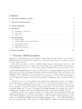
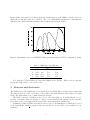
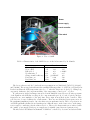
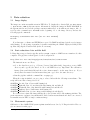
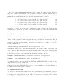
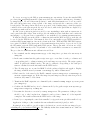
SAMI Manual
Full-frame image of planetary nebula NGC 2440 in Hα filter taken with SAMI on February 26, 2013. Exposure
time 60 s, FWHM resolution 0.32′′ , binning 2x2.
Prepared by: A. Tokovinin
Version: 1
Date: March 13, 2013
File: soar/SAMI/doc/sami-manual.tex
1
Contents
1 Overview: SAMI at a glance
2
2 Detector and electronics
3
3 Image acquisition
5
4 Geometry
4.1 Orientation on the sky . . . . . . . . . . . . . . . . . . . . . . . . . . . . . . . . . . . .
4.2 Pixel scale . . . . . . . . . . . . . . . . . . . . . . . . . . . . . . . . . . . . . . . . . . .
4.3 Distortion . . . . . . . . . . . . . . . . . . . . . . . . . . . . . . . . . . . . . . . . . . .
5
5
7
7
5 Data reduction
5.1 Image display . . . . . . .
5.2 Basic reductions: bias and
5.3 Photometric system . . .
5.4 Quick astrometry tool . .
5.5 Distortion correction . . .
8
8
8
8
9
9
. . . . .
flat field
. . . . .
. . . . .
. . . . .
.
.
.
.
.
.
.
.
.
.
.
.
.
.
.
.
.
.
.
.
6 Known problems
1
.
.
.
.
.
.
.
.
.
.
.
.
.
.
.
.
.
.
.
.
.
.
.
.
.
.
.
.
.
.
.
.
.
.
.
.
.
.
.
.
.
.
.
.
.
.
.
.
.
.
.
.
.
.
.
.
.
.
.
.
.
.
.
.
.
.
.
.
.
.
.
.
.
.
.
.
.
.
.
.
.
.
.
.
.
.
.
.
.
.
.
.
.
.
.
.
.
.
.
.
.
.
.
.
.
.
.
.
.
.
.
.
.
.
.
.
.
.
.
.
.
.
.
.
.
11
Overview: SAMI at a glance
SAMI is the CCD imager used together with the SOAR Adaptive Module, SAM. A brief overview of
SAMI given in this Section should be sufficient for writing proposals, while more details are found in
the rest of this document.
The CCD detector has a format of 4096(H)×4112(V) pixels continuous (not a mosaic). The
physical pixel size is 15×15 µm or image area 61.4×61.4 mm. The chip is CCD231-84 from E2V. It
is back-illuminated with astro broad-band AR coating and quantum efficiency around 90% between
500 nm and 700 nm (manufacturer’s data). The CCD is read out through 4 amplifiers using the SDSUIII (“Leach”) controller. The image is written in a multi-extension FITS file. The readout time of the
full frame without binning is about 8 s, the gain is 2.1 electrons per ADU, and the readout noise is
1.83 ADU or 3.8 el. Pattern noise is absent. The response is linear to 0.5% up to the digital saturation
at 65536 ADU (16 bit unsigned integer). The blade shutter of SAMI can realize exposures as short as
0.1 s.
The sky is projected onto the CCD through SAM without changing the effective focal length of
the SOAR telescope (68.0 m). This gives a pixel scale of 45.5 mas and the square field of view of
186′′ = 3.1′ . With nominal SAM position angle of 0◦ the +X axis (increasing pixel count along the
line) points East, +Y axis (increasing line count) points North. The angle between +Y and North
is typically within ±0.5◦ from zero, depending on the SOAR Nasmyth rotator setting. The optics of
SAM introduces quadratic distortion reaching 42 pixels in the corners of the CCD (see below).
SAMI has one filter wheel with 7 positions for 3′′ square filters. The Bessell BV RI filters are
installed permanently, the remaining 3 positions are occupied by narrow-band filters (for now Hα
only). Filter transmission curves are plotted in Fig. 1. Table 1 lists the central wavelength λ0 (midpoint between half-max), FWHM ∆λ, and maximum transmission Tmax of the SAMI BV RI filters.
The last column gives the relative efficiency of SAM+SAMI in comparison with the SOAR Optical
2
Imager (SOI), as measured by L. Fraga on the sky. In all bands except B SAMI records more photons
than SOI per unit time [photons or ADU??]. The “red” SAMI filters transmit more light than the
SOI filters, the SAM’s internal transmission at 633 nm is 0.90±0.06 (R. Tighe).
Figure 1: Transmission curves of SAMI BV RI filters (measurements by D. Hölck on August 25, 2010).
Table 1: SAMI filters and efficiency
Filt
λ0
∆λ Tmax , % SAMI/SOI
B
4342 984
58.3
0.71
V
5371 892
72.5
1.01
R
6441 1536
76.9
1.58
I
8103 1429
93.8
1.16
Note that the UV laser light at 355 nm leaks slightly in the B filter. This is seen as extra sky
background with a dark “cross” at the center.
2
Detector and electronics
The CCD is housed in a liquid nitrogen dewar fabricated at CTIO. The hold time is more than 24 h.
The window in front of the ccd is made of fused silica, has 9 mm thickness and is AR-coated with
MgF2 . The CCD surface is at ∼ 4 mm behind the window.
The SDSU controller of SAMI is located close to the dewar (Fig. 2). It works without cover to
prevent over-heating. Therefore the glycol cooling does not extract the heat generated by the controller
(as well as by its power supply) and it degrades the environment in the SOAR dome.
Preliminary results of CCD tests in the laboratory (prior to the installation on SAM) are reported
by R. Schmidt (file SAMI acceptance1.xls) and reproduced below in Table 2 (n/a stands for nonavailable).
3
Dewar
Power supply
Leach controller
Filter wheel
Figure 2: View of SAMI.
Table 2: Characteristics of the SAMI detector in the lab measured by R. Schmidt
Parameter
Gain, el/ADU
Noise, ADU
Full well, el
Non-linearity, %
Charge transfer efficiency
Pixel time, µs
Dwell time, ns
Slow
0.66
3.71
n/a
n/a
n/a
5.20
2120
Normal
2.1
1.83
n/a
n/a
≥0.9999927
2.320
680
Fast
4.85
1.27
> 200kel
<0.5
n/a
1.60
320
The detector has several “hot” pixels, the most prominent are at [1961,1962], [707,1553], [911,696],
and [744,402]. The average dark current at the nominal CCD temperature of −120◦ C is ≤2 el/pixel/hour.
It was found that the CCD temperature rises by ∼ 5◦ when the chip is not clocked (e.g. during long
exposures). Otherwise, the long-term stability of the temperature control is ±1◦ or better.
No pattern noise in the bias images was noticed in the initial lab tests. However, Fourier spectrum
of the signal in each CCD line reveals periodic components with periods of 5 and 2.5 pixels. As these
frequencies are exact multiples of the pixel time, their origin is most likely in the controller. This
periodic noise does not dominate the overall variance. There is some additional low-frequency noise in
the quadrants (amplifiers) 1 and 2, but only white noise in quadrants 3 and 4. Table 3 reports noise in
each CCD quadrant calculated from bias images in 3 different ways: on the bias section, on the image
section, and by considering only the white-noise floor. These noise characteristics were achieved with
the “small” power supply (a larger power supply used originally caused increased pattern noise).
The filter wheel and shutter mechanisms of SAMI are controlled by electronic modules in SAM.
4
Table 3: Noise in SAMI (ADU rms per quadrant, normal mode)
Condition
Bias section
Image
Noise floor
Q1
1.85
2.54
1.78
Q2
1.99
2.84
1.84
Q3
2.13
2.12
1.50
Q4
1.42
2.05
1.97
When SAM electronics is powered off, SAMI cannot be used.
The filter wheel of SAMI is designed to be interchangeable with the wheel of SOI, which has
5 positions with 4′′ square filters. Such wheel swap has not been tested yet. To remove the filter
wheel, disconnect its motor and free the holding screw on the left side of the wheel. Be careful not to
damage the cables that obstruct access to the wheel (Fig. 2). It is a good idea to select empty filter
before removing the wheel, thus protecting the filters from occasional damage. After each filter-wheel
manipulation, the dust on the filters changes and new flat-field calibrations must be taken.
3
Image acquisition
The SAMI data acquisition software runs on the soarhrc computer (IP 139.229.15.163). It is accessed
by VNC connection to soarhrc:9. To launch the SAMI GUI, use the icon in the desktop menu in the
lower-right corner.
The SAMI software was cloned from SOI, it is nearly identical. Figure 3 is a screen-shot of the
SAMI GUI (the instrument was switched off when it was taken). The GUI is self-explanatory. Its upper
part shows information on temperatures, information from the TCS, progress of current exposure and
readout, and current detector geometry (binning and ROI). Just below, we enter the data directory
like /home2/images/20130225 and base file name like soar20130225. The lower-left part (greyed out
in the figure) is used to set the object name, exposure duration, and the number of exposures. The
lower-right panel changes the filters: select the new filter, then press Move, and verify that it actually
changed.
The buttons in the bottom part of the GUI activate respective plug-ins, opening additional windows. See the future document on SAMI software for details.
Each acquired image can be immediately displayed if the DS9 program is running and if the realtime display is enabled in the Misc plug-in of SAMI GUI. Note however that this display has some
problems and that the pixel coordinates shown by this display are different from the true coordinates.
We recommend to disable the real-time display and to examine the images using IRAF.
Use the button Exit in the upper right to exit the software (this is recommended for easing the
load on TCS connections while SAMI is not used). If this does not work (e.g. when the SAMI GUI
hangs), kill the window. Then open the terminal, check for Labview processes with the command ps
-ax and kill the Labview process corresponding to SAMI to finish the “dirty” exit.
4
4.1
Geometry
Orientation on the sky
The position angle of the Nasmyth rotator is not written in the FITS headers of the SAMI images.
Instead, they contain the keywords RAPANGL and DECPANGL. According to the mosaic FITS
5
Figure 3: GUI of the SAMI data-taking software.
convention,1 these keywords indicate the position angle of the RA and DEC axes relative to the
+Y-axis of the CCD, counting positive CCW. For SAMI, the correct relations are:
DECP AN GL = P A
RAP AN GL = P A − 90
(1)
(2)
The keywords in the SAMI headers actually correspond to these relations. For example, the image
mzfsoar20121203.028.fits has
1
http://iraf.noao.edu/projects/ccdmosaic/imagedef/fitsdic.html
6
RAPANGL =
DECPANGL=
-270. / Position angle of RA axis (deg)
-180. / Position angle of DEC axis (deg)
which corresponds to PA=−180. In this case RAPANGL = 90 would be also correct.
The actual orientation of SAM frames on the sky can differ by as much as ±0.5◦ from the nominal
orientation. This was determined by linear astrometric solutions with quickastrometry. Depending
on the density of stars, the North direction relative to the SAMI +Y axis, θN orth , is determined
with standard errors between 0.2◦ and 0.3◦ . The accuracy increases to 0.1◦ when SAMI image is
corrected for distortion (see below). The SAM guider +Y axis is rotated w.r.t. SAMI +Y axis by
θSAM I = +0.12◦ , as determined by imaging the fiber light source in SAMI at various positions.
4.2
Pixel scale
The pixel scale of SAMI is 45.5 ± 0.05 mas, as determined by quickastrometry. With 15 µm pixels,
this corresponds to the effective telescope focal length of 68.00 m.
The pixel scale corresponds to CDELT of 1.2639E-5 degrees per pixel. However, this keyword is not
used by FITS nowadays, being replaced by the matrix CD that transforms pixels to degrees on the sky.
Combining the scale and orientation, the elements of this matrix should be set for SAMI to:
CD1 1 = 1.2639E − 5 × cos θ
(3)
CD2 2 = 1.2639E − 5 × cos θ
(4)
CD1 2 = 1.2639E − 5 × sin θ
(5)
CD2 1 = −1.2639E − 5 × sin θ
(6)
where θ = DECPANGL = PA for SAMI. The non-diagonal terms CD1 2 and CD2 1 become leading
when the position angle is 90◦ or 270◦ .
4.3
Distortion
The re-imaging system of SAM has substantial distortion, reaching 42 pixels (1.93′′ on the sky) in the
corners of the image. It was studied in the SDN 2325 by measuring pixel coordinates of point light
sources on the guide probes that were placed at different positions in the field using the XY stages
(these measures were repeated on March 4, 2013 and confirmed the previous result). The distortion
is well described by quadratic terms in X and Y:
∆x = cxx (x − x0 )2 + cxy (y − y0 )2
2
2
∆y = cyx (x − x0 ) + cyy (y − y0 ) ,
(7)
(8)
where ∆x and ∆y are the corrections to the star position (in pixels) to be added for removing the
distortion, x and y are the measured star coordinates, x0 = 2048 and y0 = 2056 are the CCD centers.
All coordinates here are determined in original, un-binned pixels. The coefficients are determined to
be cxx = 2.00E − 6, cxy = 2.15E − 6, cyx = −4.24E − 6, cyy = −4.37E − 6.
Unlike classical radial distortion in optical instruments, the distortion in SAMI moves stars in the
same direction – down and to the right – in all corners of the field. Ways to account for the distortion
are discussed in Sect. 5.5 below.
7
5
Data reduction
5.1
Image display
The images are written as multi-extension FITS files. To display those data in DS9, use Open Other
-- Open Mosaic IRAF in the File menu. Alternatively, display the images in IRAF. Run IRAF in
the xgterm window and load the packages >iraf>ecl>mscred to work with mosaic images. Also do
not forget the command >set imt=4096 at the beginning. Go to the image directory and use the
following typical commands:
mscdisplay soar20130225.0037.fits [zs- zr- z1=0 z2=40000]
mscexam
Note that star coordinates and FWHM are reported by IRAF in un-binned pixels even for images
with binning. To show image in standard orientation matching the GMAP display in SAM (North
up, East left), flip the X-axis in DS9 (in the Zoom menu).
5.2
Basic reductions: bias and flat field
L. Fraga has set up a reduction pipeline at the soarpd1 computer. SAMI data are transferred to this
computer. The pipeline works in pyraf. See the description at:
http://www.ctio.noao.edu/~fraga/pysoar/tasks/sami/doc/cookbook.html
The instructions are as follows:
• Go to the data directory (e.g. cd /home/observer/data/2012-03-01). Suggestion: create a RED
directory and copy all your data to it. Go to the RED directory. Important! The calibration
frames (biases and flat-fields) and the science frames must be in the same directory. If you
already have the master bias and master flats, just copy both to the same directory.
• Run the pipeline with the command line: soipipe.py
When the script is finished you are going to reduced files with the following nomenclature. The
script will create lists of images as below:
0SAMIList Zero1x1: List of biases with binning 1x1
1SAMIList Flat1x1B: List of dome flat-fields with binning 1x1 and filter B
2SAMIList SFlat1x1B: List of sky flat-fields with binning 1x1 and filter B
3SAMIList Dark1x1: List of dark frames with binning 1x1
4SAMIList OBJ1x1B: List of science images with binning 1x1 and filter B.
For a raw science frame like image.001.fits, the reduced frame will be like mzfimage.001.fits. The
prefix z means zero subtract, f means flat-field divided and m means that the file has been converted
from multi-extesion FITS to single continuous image.
5.3
Photometric system
Calibration of the SAMI BV RI system against standards was done by L. Fraga in 2012.2 Here we
give an extract from his paper.
2
Fraga, L. et al., 2013, AJ, submitted
8
In order to transform instrumental magnitudes and colors into the standard system, calibration
images were obtained with SAMI (in open loop) under photometric conditions during the night of
2012 June 6. The zeropoint, color terms, and extinction were determined using the IRAF package
photcal through a uniformly weighted fit of the following transformation equations:
b = B − (0.06 ± 0.03) − (0.21 ± 0.01)(B − V ) + (0.18 ± 0.02) X,
(9)
v = V − (0.48 ± 0.01) + (0.01 ± 0.01)(V − R) + (0.11 ± 0.01) X,
(10)
r = R − (0.79 ± 0.01) − (0.03 ± 0.01)(V − R) + (0.04 ± 0.01) X,
(11)
= I − (0.16 ± 0.01) − (0.07 ± 0.01)(R − I) + (0.02 ± 0.01) X,
(12)
i
where B, V , R, and I are the magnitudes in the standard system, b, v, r, and i are the instrumental
magnitudes, corrected to the exposure time of 1 s using a zero point of 25.0 mag, and X is the air-mass
at the time of the observations. The r.m.s. deviations from the fits were 0.013, 0.013, 0.010 and 0.018
mag in B, V, R, and I, respectively.
5.4
Quick astrometry tool
L. Fraga created a python script samiqastrometry.py to determine offset and angle of SAMI images
by referencing to star catalogs. It is based on the autoastrometry.py by D. Perley which compares
“blindly” stellar configurations in the image with the catalog and finds the orientation and offset. It
starts by running the sextractor to create a list of stars with pixel coordinates and magnitudes. The
sextractor and python packages numpy, pyfits have to be installed to use this tool. It is called
from the command line as
./samiastrometry.py mzfsoar20121203.026.fits -px 0.0455 -c tmc
if the 2MASS catalog is used. Astrometric information is encoded in the FITS header in the form
of RA—TAN and DEC–TAN WCS keywords (linear transformation from pixels to RA,DEC). The
image with modified header is saved in the separate file with the ’a’ prefix. At the end of the header,
the rms difference between catalog and star centroids and the rotation are listed as:
ASTR_UNC=
ASTR_SPA=
ASTR_DPA=
0.09891016893935835 / Astrometric scatter vs. catalog (arcsec)
0.09456702004780501 / Measured uncertainty in PA (degrees)
-180.749724946754 / Change in PA (degrees)
The ASTR DPA angle is counted from the Y-axis CCW, same at DECPANGL. The procedure does not
change the pixel scale in the FITS header!
We note that the SAMI data in December 2012 had PA offset of −0.8◦ , while this offset was +0.2◦
in March and May 2012. The SOAR TCS therefore does not maintain a very accurate alignment of
the Nasmyth rotator with celestial coordinates.
5.5
Distortion correction
The ways to deal with distortion in SAMI depend on the goals. Distortion prevents simple co-addition
of dithered images or mosaicing. In this case, images must be re-binned into undistorted pixels before
recombination. If, on the other hand, we just want to do astrometry, correcting the world coordinate
system (WCS) in the FITS header is the best way to proceed.
9
For image un-wrapping, the IDL program samiwrap.pro was written. It uses the standard IDL
procedure poly 2d and implements the equations 8, where the polynomial coefficients were determined
by samipoly.pro. We use bi-linear interpolation to make this transformation as “local” as possible
(the cubic interpolation uses a larger patch of the image and spreads the cosmic-ray events over
several pixels). The interpolation affects noise properties of the resulting image: when the signal is
combined from several adjacent pixels, the noise is reduced, while in the pixels that are displaced by
a near-integer number the noise is not affected.
If a list of star positions in pixels is created by some star-finding routine such as sextractor, it
can be passed through a “filter” that would produce the undistorted list. Such filter can be written in
any language, e.g. in pyraf. It is recommendable to use such filter before running quickastrometry.
Non-linear relation between the CCD coordinates in pixels and the WCS in degrees on the sky can
be encoded in the FITS header. Unfortunately, there is no universally accepted FITS standard for
non-linear WCS transformations. One such convention, the RA—TNX and DEC–TNX WCS system,
is recognized by IRAF.3 The linear part of the transformation from pixels to degrees is encoded in
the CD matrix, as in the TNG (tangential) WCS system. Then polynomial corrections are added,
defined by the WATj nnn keywords. Polynomials of order 3 with half cross-terms are recommended.
The procedure for SAMI astrometric calibration is as follows.
1. In a terminal, run the samiqastrometry.py on the image.fits to get first-order astrometry in
aimage.fits
2. In the same terminal run the python script scat.py to create lists of catalog coordinates and
corresponding pixel coordinates in image.radec and image.xy respectively. The script requires
astLib. It queries the 2MASS catalog. The pixel coordinates corresponding to the catalogued
stars are calculated from the information in the FITS header.
3. The following steps are executed in IRAF. Load the packages digiphot and appphot. Display
the image, mark the stars by >tvmark coord=image.xy label- mark=circle.
4. Find centroids of the stars by the IRAF command >center aimage.fits coords=image.xy
cbox=25 output=image1.xy. If the files image1.xy and image2.xy already exist from previous
iterations, they must be deleted first.
5. Transform the IRAF output into a 2-column file by the command >txdump image1.xy xcent,ycent
yes >image2.xy
6. Combine the RA,DEC and x,y in a 5-column text file by the python script side-by-side.py
image.radec image2.xy >ccdmap.dat
7. Determine the distortion correction by >ccmap aimage.fits. The parameters of this procedure
should be set to take long,lat from columns 1,2 and x,y from columns 4,5 of the input file
ccmap.dat. The result is written in the FITS header of the image.
8. Iterate by re-computing the centroids in a smaller box (repeat from step 4 with a smaller cbox).
Application of this procedure results in the rms residuals from 0.04′′ (1 pixel) to 0.07′′ .
In principle, it is possible to provide a first-order distortion correction in the raw images by precalculating the polynomials in WATj nnn. The difficulty is that these transformations are defined in
3
http://iraf.noao.edu/projects/ccdmosaic/tnx.html
10
the sky coordinates (degrees), not in pixels. Therefore, the coefficients will depend on the position
angle. They can be pre-calculated for the 4 standard position angles.
6
Known problems
Problems with SAMI or its data that were encountered during its short lifetime are listed without
specific order.
• The SAMI GUI “freezes”, no reaction to commands. Dirty exit and re-start normally help.
• Filters do not move or do not reach position. Try to send the Move command again. If the wheel
still does not move, it may be really stuck. Balancing the filters (avoid several open positions
on one side) might help.
• During VNC connection to SAMI, the screen “freezes” and the cursor is replaced by a cross.
This usually happens after moving windows. Wait for 30 s, the normal cursor comes back again.
• SAMI gets no light. Check that SOAR is opened and configured for SAM (M3 position and M4
in the ISB), that the SAM environmental shutter is open, and that the SAM output selector
mirror is in the SAMI position. A point light source in the SAM guide probe can be placed at
center and imaged for a test.
• Deep images in the B filter show a dark “cross” in the middle and increased background. This
is the scattered laser light at 355 nm that leaks through SAM dichroic and B filter. Nothing can
be done about it now.
• Deep images in the V filter show a gradient of the background. This is caused by a light source
in the SOAR ISB. Eventually this will be eliminated.
• The star images have cometary “tails” on one side or several fainter “rays”. These defects are
caused by the SAM AO system, they are reduced by proper tuning of the SAM AO loop.
• Stars have bright long tails. This is caused by divergence of the SAM tip-tilt guiding loop due
to wrong information received from the TCS. Discard those images.
11