1
Failures-Divergence Refinement
FDR2 User Manual
19th October 2010
Formal Systems (Europe) Ltd
<http://www.fsel.com/>
Oxford University Computing Laboratory
<http://web.comlab.ox.ac.uk/projects/concurrency-tools/>
c 1992–2005 Formal Systems (Europe) Ltd, 2009–2010 Oxford University
Copyright This is the ninth edition of this User Manual.
It covers primarily FDR version 2.91.
i
Table of Contents
.......................................................... 1
Acknowledgements . . . . . . . . . . . . . . . . . . . . . . . . . . . . . . . . . . . . . . . . 2
1
Introduction . . . . . . . . . . . . . . . . . . . . . . . . . . . . . . . . . . . . . . . . . . . 3
1.1
1.2
1.3
1.4
2
What is FDR? . . . . . . . . . . . . . . . . . . . . . . . . . . . . . . . . . . . . . . . . . . . . . . . . . . . . . . . . . . . .
The CSP View of the World . . . . . . . . . . . . . . . . . . . . . . . . . . . . . . . . . . . . . . . . . . . . . . . .
CSP Refinement. . . . . . . . . . . . . . . . . . . . . . . . . . . . . . . . . . . . . . . . . . . . . . . . . . . . . . . . . . .
1.3.1 Using refinement . . . . . . . . . . . . . . . . . . . . . . . . . . . . . . . . . . . . . . . . . . . . . . . . . .
1.3.2 Simple buffer example . . . . . . . . . . . . . . . . . . . . . . . . . . . . . . . . . . . . . . . . . . . . .
1.3.3 Checking refinement . . . . . . . . . . . . . . . . . . . . . . . . . . . . . . . . . . . . . . . . . . . . . .
Specification Example . . . . . . . . . . . . . . . . . . . . . . . . . . . . . . . . . . . . . . . . . . . . . . . . . . . . .
1.4.1 Multiplexed buffer example . . . . . . . . . . . . . . . . . . . . . . . . . . . . . . . . . . . . . . . .
Using FDR . . . . . . . . . . . . . . . . . . . . . . . . . . . . . . . . . . . . . . . . . . . 11
2.1
2.2
2.3
The Main Window . . . . . . . . . . . . . . . . . . . . . . . . . . . . . . . . . . . . . . . . . . . . . . . . . . . . . . .
On-line Help . . . . . . . . . . . . . . . . . . . . . . . . . . . . . . . . . . . . . . . . . . . . . . . . . . . . . . . . . . . . .
File and Model Commands . . . . . . . . . . . . . . . . . . . . . . . . . . . . . . . . . . . . . . . . . . . . . . . .
2.3.1 The Load command . . . . . . . . . . . . . . . . . . . . . . . . . . . . . . . . . . . . . . . . . . . . . .
2.3.2 The Reload command . . . . . . . . . . . . . . . . . . . . . . . . . . . . . . . . . . . . . . . . . . . .
2.3.3 The Edit command . . . . . . . . . . . . . . . . . . . . . . . . . . . . . . . . . . . . . . . . . . . . . .
2.3.4 The All Asserts command . . . . . . . . . . . . . . . . . . . . . . . . . . . . . . . . . . . . . . . .
2.3.5 The Exit command . . . . . . . . . . . . . . . . . . . . . . . . . . . . . . . . . . . . . . . . . . . . . .
2.4 The Assertion List . . . . . . . . . . . . . . . . . . . . . . . . . . . . . . . . . . . . . . . . . . . . . . . . . . . . . . .
2.5 The Process List . . . . . . . . . . . . . . . . . . . . . . . . . . . . . . . . . . . . . . . . . . . . . . . . . . . . . . . . .
2.6 The Tab Pane . . . . . . . . . . . . . . . . . . . . . . . . . . . . . . . . . . . . . . . . . . . . . . . . . . . . . . . . . . . .
2.7 Options . . . . . . . . . . . . . . . . . . . . . . . . . . . . . . . . . . . . . . . . . . . . . . . . . . . . . . . . . . . . . . . . .
2.8 Tab Bar Commands . . . . . . . . . . . . . . . . . . . . . . . . . . . . . . . . . . . . . . . . . . . . . . . . . . . . . .
2.9 The FDR Process Debugger . . . . . . . . . . . . . . . . . . . . . . . . . . . . . . . . . . . . . . . . . . . . . . .
2.9.1 Debugger menu commands . . . . . . . . . . . . . . . . . . . . . . . . . . . . . . . . . . . . . . .
2.9.2 Viewing process behaviours . . . . . . . . . . . . . . . . . . . . . . . . . . . . . . . . . . . . . . .
2.9.2.1 The process structure. . . . . . . . . . . . . . . . . . . . . . . . . . . . . . . . . . . .
2.9.2.2 The behaviour information . . . . . . . . . . . . . . . . . . . . . . . . . . . . . . .
2.10 Interface Conventions . . . . . . . . . . . . . . . . . . . . . . . . . . . . . . . . . . . . . . . . . . . . . . . . . . . .
2.10.1 GUI conventions . . . . . . . . . . . . . . . . . . . . . . . . . . . . . . . . . . . . . . . . . . . . . . . .
2.10.2 Keyboard short-cuts . . . . . . . . . . . . . . . . . . . . . . . . . . . . . . . . . . . . . . . . . . . .
3
3
3
5
6
7
7
8
8
11
12
12
12
13
13
13
13
13
14
15
16
16
17
17
17
17
18
19
19
19
Tutorial . . . . . . . . . . . . . . . . . . . . . . . . . . . . . . . . . . . . . . . . . . . . . . 20
3.1
3.2
Describing Processes . . . . . . . . . . . . . . . . . . . . . . . . . . . . . . . . . . . . . . . . . . . . . . . . . . . . . .
3.1.1 Sample script for FDR2 . . . . . . . . . . . . . . . . . . . . . . . . . . . . . . . . . . . . . . . . . .
Using the Checker . . . . . . . . . . . . . . . . . . . . . . . . . . . . . . . . . . . . . . . . . . . . . . . . . . . . . . . .
3.2.1 Environment . . . . . . . . . . . . . . . . . . . . . . . . . . . . . . . . . . . . . . . . . . . . . . . . . . . .
3.2.2 Getting started . . . . . . . . . . . . . . . . . . . . . . . . . . . . . . . . . . . . . . . . . . . . . . . . . .
3.2.3 Debugging . . . . . . . . . . . . . . . . . . . . . . . . . . . . . . . . . . . . . . . . . . . . . . . . . . . . . .
20
22
23
23
24
25
ii
4
Intermediate FDR. . . . . . . . . . . . . . . . . . . . . . . . . . . . . . . . . . . . . 30
4.1
4.2
4.3
5
Building a Model . . . . . . . . . . . . . . . . . . . . . . . . . . . . . . . . . . . . . . . . . . . . . . . . . . . . . . . . .
4.1.1 Abstract model . . . . . . . . . . . . . . . . . . . . . . . . . . . . . . . . . . . . . . . . . . . . . . . . . .
4.1.2 Use components . . . . . . . . . . . . . . . . . . . . . . . . . . . . . . . . . . . . . . . . . . . . . . . . .
Tuning for FDR . . . . . . . . . . . . . . . . . . . . . . . . . . . . . . . . . . . . . . . . . . . . . . . . . . . . . . . . . .
4.2.1 Share components . . . . . . . . . . . . . . . . . . . . . . . . . . . . . . . . . . . . . . . . . . . . . . .
4.2.2 Factor state . . . . . . . . . . . . . . . . . . . . . . . . . . . . . . . . . . . . . . . . . . . . . . . . . . . . .
4.2.3 Use local definitions . . . . . . . . . . . . . . . . . . . . . . . . . . . . . . . . . . . . . . . . . . . . . .
Choice of Model . . . . . . . . . . . . . . . . . . . . . . . . . . . . . . . . . . . . . . . . . . . . . . . . . . . . . . . . . .
30
30
30
31
31
32
32
33
Advanced Topics . . . . . . . . . . . . . . . . . . . . . . . . . . . . . . . . . . . . . . 34
5.1
5.2
Using Compressions . . . . . . . . . . . . . . . . . . . . . . . . . . . . . . . . . . . . . . . . . . . . . . . . . . . . . .
5.1.1 Methods of compression . . . . . . . . . . . . . . . . . . . . . . . . . . . . . . . . . . . . . . . . . .
5.1.2 Compressions in context . . . . . . . . . . . . . . . . . . . . . . . . . . . . . . . . . . . . . . . . . .
5.1.3 Hiding and safety properties . . . . . . . . . . . . . . . . . . . . . . . . . . . . . . . . . . . . . .
5.1.4 Hiding and deadlock . . . . . . . . . . . . . . . . . . . . . . . . . . . . . . . . . . . . . . . . . . . . .
Technical Details . . . . . . . . . . . . . . . . . . . . . . . . . . . . . . . . . . . . . . . . . . . . . . . . . . . . . . . . .
5.2.1 Generalised Transition Systems . . . . . . . . . . . . . . . . . . . . . . . . . . . . . . . . . . .
5.2.2 State-space Reduction . . . . . . . . . . . . . . . . . . . . . . . . . . . . . . . . . . . . . . . . . . . .
5.2.2.1 Computing semantic equivalence . . . . . . . . . . . . . . . . . . . . . . . . .
5.2.2.2 Diamond elimination . . . . . . . . . . . . . . . . . . . . . . . . . . . . . . . . . . . .
5.2.2.3 Combining techniques . . . . . . . . . . . . . . . . . . . . . . . . . . . . . . . . . . .
34
34
35
36
36
37
37
38
39
40
41
Appendix A Syntax Reference . . . . . . . . . . . . . . . . . . . . . . . . . . . . 43
A.1
A.2
A.3
A.4
A.5
A.6
A.7
A.8
Expressions . . . . . . . . . . . . . . . . . . . . . . . . . . . . . . . . . . . . . . . . . . . . . . . . . . . . . . . . . . . . .
A.1.1 Identifiers . . . . . . . . . . . . . . . . . . . . . . . . . . . . . . . . . . . . . . . . . . . . . . . . . . . . . .
A.1.2 Numbers . . . . . . . . . . . . . . . . . . . . . . . . . . . . . . . . . . . . . . . . . . . . . . . . . . . . . . .
A.1.3 Sequences . . . . . . . . . . . . . . . . . . . . . . . . . . . . . . . . . . . . . . . . . . . . . . . . . . . . . .
A.1.4 Sets . . . . . . . . . . . . . . . . . . . . . . . . . . . . . . . . . . . . . . . . . . . . . . . . . . . . . . . . . . . .
A.1.5 Booleans . . . . . . . . . . . . . . . . . . . . . . . . . . . . . . . . . . . . . . . . . . . . . . . . . . . . . . .
A.1.6 Tuples . . . . . . . . . . . . . . . . . . . . . . . . . . . . . . . . . . . . . . . . . . . . . . . . . . . . . . . . . .
A.1.7 Local definitions . . . . . . . . . . . . . . . . . . . . . . . . . . . . . . . . . . . . . . . . . . . . . . . .
A.1.8 Lambda terms . . . . . . . . . . . . . . . . . . . . . . . . . . . . . . . . . . . . . . . . . . . . . . . . . .
Pattern Matching . . . . . . . . . . . . . . . . . . . . . . . . . . . . . . . . . . . . . . . . . . . . . . . . . . . . . . . .
Types . . . . . . . . . . . . . . . . . . . . . . . . . . . . . . . . . . . . . . . . . . . . . . . . . . . . . . . . . . . . . . . . . . .
A.3.1 Simple types . . . . . . . . . . . . . . . . . . . . . . . . . . . . . . . . . . . . . . . . . . . . . . . . . . . .
A.3.2 Named types. . . . . . . . . . . . . . . . . . . . . . . . . . . . . . . . . . . . . . . . . . . . . . . . . . . .
A.3.3 Datatypes . . . . . . . . . . . . . . . . . . . . . . . . . . . . . . . . . . . . . . . . . . . . . . . . . . . . . .
A.3.4 Subtypes . . . . . . . . . . . . . . . . . . . . . . . . . . . . . . . . . . . . . . . . . . . . . . . . . . . . . . .
A.3.5 Channels . . . . . . . . . . . . . . . . . . . . . . . . . . . . . . . . . . . . . . . . . . . . . . . . . . . . . . .
A.3.6 Closure operations . . . . . . . . . . . . . . . . . . . . . . . . . . . . . . . . . . . . . . . . . . . . . .
Processes. . . . . . . . . . . . . . . . . . . . . . . . . . . . . . . . . . . . . . . . . . . . . . . . . . . . . . . . . . . . . . . .
Operator Precedence . . . . . . . . . . . . . . . . . . . . . . . . . . . . . . . . . . . . . . . . . . . . . . . . . . . . .
Special Definitions . . . . . . . . . . . . . . . . . . . . . . . . . . . . . . . . . . . . . . . . . . . . . . . . . . . . . . .
A.6.1 External . . . . . . . . . . . . . . . . . . . . . . . . . . . . . . . . . . . . . . . . . . . . . . . . . . . . . . . .
A.6.2 Transparent . . . . . . . . . . . . . . . . . . . . . . . . . . . . . . . . . . . . . . . . . . . . . . . . . . . .
A.6.3 Assert . . . . . . . . . . . . . . . . . . . . . . . . . . . . . . . . . . . . . . . . . . . . . . . . . . . . . . . . . .
A.6.4 Print . . . . . . . . . . . . . . . . . . . . . . . . . . . . . . . . . . . . . . . . . . . . . . . . . . . . . . . . . . .
Mechanics . . . . . . . . . . . . . . . . . . . . . . . . . . . . . . . . . . . . . . . . . . . . . . . . . . . . . . . . . . . . . . .
Missing Features . . . . . . . . . . . . . . . . . . . . . . . . . . . . . . . . . . . . . . . . . . . . . . . . . . . . . . . . .
43
44
44
45
46
47
48
48
49
50
52
52
52
53
53
54
55
56
59
60
60
60
60
61
62
62
iii
Appendix B Changes to FDR . . . . . . . . . . . . . . . . . . . . . . . . . . . . 64
B.1
B.2
B.3
B.4
B.5
B.6
B.7
B.8
B.9
B.10
B.11
B.12
B.13
B.14
B.15
B.16
B.17
B.18
B.19
B.20
B.21
B.22
Changes from FDR1 to FDR2 . . . . . . . . . . . . . . . . . . . . . . . . . . . . . . . . . . . . . . . . . . . .
Changes from 2.0 to 2.1 . . . . . . . . . . . . . . . . . . . . . . . . . . . . . . . . . . . . . . . . . . . . . . . . . .
Changes from 2.1 to 2.20 . . . . . . . . . . . . . . . . . . . . . . . . . . . . . . . . . . . . . . . . . . . . . . . . .
Changes from 2.20 to 2.22 . . . . . . . . . . . . . . . . . . . . . . . . . . . . . . . . . . . . . . . . . . . . . . . .
Changes from 2.22 to 2.23 . . . . . . . . . . . . . . . . . . . . . . . . . . . . . . . . . . . . . . . . . . . . . . . .
Changes from 2.23 to 2.24 . . . . . . . . . . . . . . . . . . . . . . . . . . . . . . . . . . . . . . . . . . . . . . . .
Changes from 2.24 to 2.25 . . . . . . . . . . . . . . . . . . . . . . . . . . . . . . . . . . . . . . . . . . . . . . . .
Changes from 2.25 to 2.26 . . . . . . . . . . . . . . . . . . . . . . . . . . . . . . . . . . . . . . . . . . . . . . . .
Changes from 2.26 to 2.27 . . . . . . . . . . . . . . . . . . . . . . . . . . . . . . . . . . . . . . . . . . . . . . . .
Changes from 2.27 to 2.28 . . . . . . . . . . . . . . . . . . . . . . . . . . . . . . . . . . . . . . . . . . . . . . .
Changes from 2.28 to 2.64 . . . . . . . . . . . . . . . . . . . . . . . . . . . . . . . . . . . . . . . . . . . . . . .
Changes from 2.64 to 2.68 . . . . . . . . . . . . . . . . . . . . . . . . . . . . . . . . . . . . . . . . . . . . . . .
Changes from 2.68 to 2.69 . . . . . . . . . . . . . . . . . . . . . . . . . . . . . . . . . . . . . . . . . . . . . . .
Changes from 2.69 to 2.76 . . . . . . . . . . . . . . . . . . . . . . . . . . . . . . . . . . . . . . . . . . . . . . .
Changes from 2.76 to 2.77 . . . . . . . . . . . . . . . . . . . . . . . . . . . . . . . . . . . . . . . . . . . . . . .
Changes from 2.77 to 2.78 . . . . . . . . . . . . . . . . . . . . . . . . . . . . . . . . . . . . . . . . . . . . . . .
Changes from 2.78 to 2.80 . . . . . . . . . . . . . . . . . . . . . . . . . . . . . . . . . . . . . . . . . . . . . . .
Changes from 2.80 to 2.81 . . . . . . . . . . . . . . . . . . . . . . . . . . . . . . . . . . . . . . . . . . . . . . .
Changes from 2.81 to 2.82 . . . . . . . . . . . . . . . . . . . . . . . . . . . . . . . . . . . . . . . . . . . . . . .
Changes from 2.82 to 2.83 . . . . . . . . . . . . . . . . . . . . . . . . . . . . . . . . . . . . . . . . . . . . . . .
Changes from 2.83 to 2.90 . . . . . . . . . . . . . . . . . . . . . . . . . . . . . . . . . . . . . . . . . . . . . . .
Changes from 2.90 to 2.91 . . . . . . . . . . . . . . . . . . . . . . . . . . . . . . . . . . . . . . . . . . . . . . .
64
65
65
65
65
65
66
66
66
66
67
67
67
67
67
67
67
68
68
68
68
68
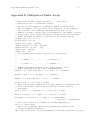
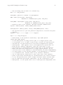
Appendix C Direct control of FDR . . . . . . . . . . . . . . . . . . . . . . . 70
C.1
C.2
C.3
Batch interface . . . . . . . . . . . . . . . . . . . . . . . . . . . . . . . . . . . . . . . . . . . . . . . . . . . . . . . . . .
Script interface . . . . . . . . . . . . . . . . . . . . . . . . . . . . . . . . . . . . . . . . . . . . . . . . . . . . . . . . . .
Object model . . . . . . . . . . . . . . . . . . . . . . . . . . . . . . . . . . . . . . . . . . . . . . . . . . . . . . . . . . . .
C.3.1 Notes on the object model . . . . . . . . . . . . . . . . . . . . . . . . . . . . . . . . . . . . . . .
C.3.2 Session objects . . . . . . . . . . . . . . . . . . . . . . . . . . . . . . . . . . . . . . . . . . . . . . . . . .
C.3.3 Ism objects . . . . . . . . . . . . . . . . . . . . . . . . . . . . . . . . . . . . . . . . . . . . . . . . . . . . .
C.3.4 Hypothesis objects . . . . . . . . . . . . . . . . . . . . . . . . . . . . . . . . . . . . . . . . . . . . . .
C.3.5 FDRSet objects . . . . . . . . . . . . . . . . . . . . . . . . . . . . . . . . . . . . . . . . . . . . . . . . .
70
71
71
71
71
72
73
74
Appendix D Configuration . . . . . . . . . . . . . . . . . . . . . . . . . . . . . . . 75
D.1
D.2
Environment variables . . . . . . . . . . . . . . . . . . . . . . . . . . . . . . . . . . . . . . . . . . . . . . . . . . .
D.1.1 Location. . . . . . . . . . . . . . . . . . . . . . . . . . . . . . . . . . . . . . . . . . . . . . . . . . . . . . . .
D.1.2 Tools . . . . . . . . . . . . . . . . . . . . . . . . . . . . . . . . . . . . . . . . . . . . . . . . . . . . . . . . . . .
D.1.3 Paging . . . . . . . . . . . . . . . . . . . . . . . . . . . . . . . . . . . . . . . . . . . . . . . . . . . . . . . . .
Performance . . . . . . . . . . . . . . . . . . . . . . . . . . . . . . . . . . . . . . . . . . . . . . . . . . . . . . . . . . . . .
75
75
75
75
75
Appendix E Multiplexed Buffer Script . . . . . . . . . . . . . . . . . . . . 77
Appendix F Bibliography . . . . . . . . . . . . . . . . . . . . . . . . . . . . . . . . 79
1
c 1992-2009, Formal Systems (Europe)
The FDR tool and this User Manual are Copyright Ltd., 2009-2010 Oxford University
Acknowledgements
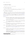
2
Acknowledgements
The development of FDR and FDR2 has received support from a number of sources.
The initial goals of the Formal Systems refinement checker were outlined by Inmos Ltd, and
an early version of the system was developed in collaboration with them. The research and
development of FDR1 was further funded in part by the US Office of Naval Research (contract
N00014–87–J1242), and ESPRIT project 2701 (PUMA).
The development of the second generation tools described here was funded in part from
internal resources, and also by contributions under contracts from the United Kingdom Defence Research Agency, ONR project N00014–93–C–0213, and as part of ESPRIT project 7267
(OMI/STANDARDS).
The research at Oxford University forming the basis of Appendix A [Syntax Reference],
page 43 was also funded under ONR contract N00014–87–J–1242. However, work beyond this
research, including the ‘compilation’ technique which closes off process terms to produce a
finite-state transition system and operations defined over such trees necessary to perform normalisation, compression and refinement-checks were all funded by Formal Systems as part of
the development of FDR and so remain the property of that company.
Since 2007 FDR2 has been maintained and developed by Oxford University Computing Laboratory with support from EPSRC project EP/E035590/1 and grants from the ONR.
This document draws together material from a number of authors, principally: Paul Gardiner,
Michael Goldsmith, Jason Hulance, David Jackson, Bill Roscoe, Bryan Scattergood and Philip
Armstrong.
Chapter 1: Introduction
3
1 Introduction
This chapter introduces the FDR tool and the CSP notation. The concept of refinement (the
heart of FDR) is discussed and some of its applications are described. The last section gives a
realistic case-study to illustrate a common use of refinement and FDR.
1.1 What is FDR?
FDR (Failures-Divergence Refinement) is a model-checking tool for state machines, with
foundations in the theory of concurrency based around CSP—Hoare’s Communicating Sequential
Processes [Hoare85]. Its method of establishing whether a property holds is to test for the
refinement of a transition system capturing the property by the candidate machine. There is
also the ability to check determinism of a state machine, and this is used primarily for checking
security properties [Roscoe95], [RosWood94]. The main ideas behind FDR are presented in
[Roscoe94] and some applications are presented in [Roscoe97].
Previous versions of the tool (up to 1.4x) used only explicit model-checking techniques: the
check proceeds by a recursion induction which fully expands the reachable state-space of the
two systems and visits each pair of supposedly corresponding states in turn. Although it is very
efficient in doing this and can deal with processes with approximately 107 states in a few hours
on a typical workstation, the exponential growth of state-space with the number of parallel
processes in a network represents a significant limit on its utility.
The primary aim in the development of the new version of the tool, FDR2, was to improve
on the flexibility and scalability of the tool. In particular, FDR2 offers
• support for operators outside the core CSP and, indeed, completely different languages
• improved handling of multi-way synchronisation, with the representation of firing rules
based on the events which components may engage in, rather than pattern-matching on
their states
• relaxation of some of the restrictions on the CSP scripts, in particular the strict distinction between “high-level” (parallel or hiding) and “low-level” (parametrised or recursive)
constructs
• provision of a much more powerful language for data types and expressions
• potential for “lazy” exploration of systems (allowing some non-finite-state specifications,
such as “is a buffer”)
• the ability to build up a system gradually, at each stage compressing the subsystems to
produce an equivalent process with (hopefully) many fewer states.
This last item means that FDR2 can check systems which are sometimes exponentially larger
than those which FDR1 can—such as a network of 1020 (or 100100 ) dining philosophers [RosEtAl95].
The “back-end” state-exploring code has been completely re-crafted. FDR2 marries this to
a new parser/compiler based on Scattergood’s implementation of the operational semantics of
CSP [Scat98]. Experimental hooks for attaching “alien” state-machine descriptions have been
developed, so it is possible for FDR2 to operate on files created by other techniques.
1.2 The CSP View of the World
CSP is a language where processes proceed from one state to another by engaging in (instantaneous) events. Processes may be composed by operators which require synchronisation on
some events; each component must be willing to participate in a given event before the whole can
Chapter 1: Introduction
4
make the transition. This, rather than assignments to shared state variables, is the fundamental
means of interaction between agents.
The composition of processes is itself a process, allowing a hierarchical description of a system.
The hiding operator makes a given set of events internal: invisible to, and beyond the control
of, its environment; this provides an abstraction mechanism.
The theory of CSP has classically been based on mathematical models remote from the
language itself. These models have been based on observable behaviours of processes such as
traces, failures and divergences, rather than attempting to capture a full operational picture of
how the process progresses.
On the other hand CSP can be given an operational semantics in terms of labelled transition
systems. This operational semantics can be related to the mathematical models: that the
standard semantics of CSP are congruent to a natural operational semantics is shown in, for
example, [Roscoe88a] and [Scat98].
Given that each of our models represents a process by the set of its possible behaviours, it
is natural to represent refinement as the reduction of these options: the reverse containment of
the set of behaviours. If Q refines P we write P v Q, sometimes subscripting v to indicate
which model the refinement it is respect to.
FDR directly supports a number of CSP models:
• The traces model: a process is represented by the set of finite sequences of communications
it can perform. The set of P ’s (finite) traces is given by traces(P ).
• The stable failures model [JateMey]: a process is represented by its traces as above and
also by its failures. A failure is a pair (s, X ), where s is a finite trace of the process (i.e., in
traces(P )) and X is a set of events it can refuse after s. This means (operationally) that
after trace s, the process P has come into a state where it can do no internal action and no
action from the set X . The set of P ’s failures is given by failures(P ).
• The failures/divergences model [BroRos85]: a process is represented by its failures as above,
together with its divergences. A divergence is a finite trace during or after which the process
can perform an infinite sequence of consecutive internal actions. The failures are extended
so that we do not care how the process behaves after any divergence.
• The refusal testing model [Lowe08]: a process is represented by a sequence of alternating
stable refusal sets and events, possibly terminating in deadlock. Unstable states, where the
process does not have a well defined refusal set are represented by \bullet.
• The revivals model [ReeRosSin07,Roscoe09]: the concept of a failure is extended with an
event a that the process might accept after completing the trace s: (s, X , a). This makes
the revivals model more discriminating than the failures model.
• Lastly the tau priority model [LowOuk05] is a variant of the traces model where a set of
events is defined as having less priority than τ . As a result, the process can only offer an
event from the defined set when it is in a stable state. One application of this is to model
the passage of time with a tock event.
All of these models have the obvious congruence theorem with the standard operational semantics of CSP. In fact FDR works chiefly in the operational world: it computes how a process
behaves by applying the rules of the operational semantics to expand it into a transition system.
The congruence theorems are thus vital in supporting all its work: it can only claim to prove
things about the abstractly-defined semantics of a process because we happen to know that this
equals the set of behaviours of the operational process FDR works with.
The congruence theorems are also fundamental in supporting the hierarchical compressions
described in Section 5.1 [Using Compressions], page 34. For we know that if C [·] is any CSP
context then the value in one of our semantic models of C [P ] depends only on the value (in the
same model) of P , not on the precise way it is represented as a transition system. Therefore, it
Chapter 1: Introduction
5
may greatly be to our advantage to find another representation of P with fewer states. If, for
example, we are combining processes P and Q in parallel and each has 1000 states, but can be
compressed to 100, the compressed composition can have no more than 10,000 states while the
uncompressed one may have up to 1,000,000.
1.3 CSP Refinement
The notion of refinement is a particularly useful concept in many forms of engineering activity.
If we can establish a relation between components of a system which captures the fact that one
satisfies at least the same conditions as another, then we may replace a worse component by a
better one without degrading the properties of the system. Obviously the notion of refinement
must reflect the properties of a system which are important: in building bridges it may acceptable
to replace a (weaker) aluminium rivet by a (stronger) iron one, but if weight is critical, say in
an aircraft, this is not a valid refinement.
In describing reactive computer systems, CSP has been found to be a useful tool. Refinement
relations can be defined for systems described in CSP in several ways, depending on the semantic
model of the language which is used. In the untimed versions of CSP, three main forms of
refinement are relevant, corresponding to the three models presented above. We briefly outline
these below, for more information see [Roscoe97].
Traces refinement
The coarsest commonly used relationship is based on the sequences of events which
a process can perform (the traces of the process). A process Q is a traces refinement
of another, P , if all the possible sequences of communications which Q can do are
also possible for P . This relationship is written P vT Q. If we consider P to be a
specification which determines possible safe states of a system, then we can think of
P vT Q as saying that Q is a safe implementation: no wrong events will be allowed.
P vT Q =
b traces(Q) ⊆ traces(P )
Traces refinement does not allow us to say anything about what will actually happen,
however. The process STOP , which never performs any events, is a refinement of
any process in this framework, and satisfies any safety specification.
Failures refinement
A finer distinction between processes can be made by constraining the events which
an implementation is permitted to block as well as those which it performs. A failure
is a pair (s, X ), where s is a trace of the process and X is a set of events the process
can refuse to perform at that point (and, to add a little more terminology, X is
called a refusal ). Failures refinement vF is defined by insisting that the set of all
failures of a refining process are included in those of the refined process.
P vF Q =
b failures(Q) ⊆ failures(P )
A state of a process is deadlocked if it can refuse to do every event, and STOP is the
simplest deadlocked process. Deadlock is also commonly introduced when parallel
processes do not succeed in synchronising on the same event.
Failures-Divergences refinement
The failures model does not allow us to easily detect one important class of states:
those after which the process might livelock (i.e., perform an infinite sequence of
internal actions) and so may never subsequently engage in a visible event. So, a
semantic model more thorough (in this respect) than the failures model is desirable.
The failures-divergences model meets this requirement by adding the concept of
divergences. The divergences of a process are the set of traces after which the
process may livelock. This gives two major enhancements: we may analyse systems
Chapter 1: Introduction
6
which have the potential to never perform another visible event and assert this does
not occur in the situations being considered; and we may also use divergence in
the specification to describe “don’t care” situations. The relation vFD is defined as
follows:
P vFD Q =
b failures(Q) ⊆ failures(P ) ∧
divergences(Q) ⊆ divergences(P )
Formally, after a divergence we consider a process to be acting chaotically and able
to do or refuse anything. This means that processes are considered to be identical
after they have diverged.
Naturally, for divergence-free processes, which include the vast majority of practical
systems, vFD is equivalent to vF .
As implied by the name of FDR, we consider vFD to be the most important of these three.
We will generally abbreviate vFD by v. The failures-divergence model, and its corresponding
notion of refinement, are usually taken as the standard model of CSP.
All three of these forms of refinement are supported in FDR. We would normally expect them
to be used in the following contexts:
• Traces refinement is used for proving safety properties.
• Failures-divergence refinement is used for proving safety, liveness and combination properties, and also for establishing refinement and equality relations between systems.
• Failures refinement is normally used to prove failures-divergence refinement for processes
that are already known to be divergence-free. It does have other uses, but these are somewhat more sophisticated. See the file ‘abp.csp’ in the FDR ‘demo’ directory for some
discussion of this issue.
1.3.1 Using refinement
A formal system supporting refinement can be used in a number of ways:
• We can develop systems by a series of stepwise refinements, starting with a specification
process and gradually refining it into an implementation. Since our notions of refinement
are all preserved by the operators of CSP, there is no need to apply refinement rules only
at the highest levels in this process. For example, if the parallel composition of P and Q
refines a specification S , written
S v P k Q,
X
then we can develop the system further by refining P and Q separately: if P v P 0 and
Q v Q 0 , then the composition of P 0 and Q 0 will also refine S :
S v P 0 k Q 0,
X
We do not need to check this condition explicitly.
• The same observation about compositionality, or monotonicity, of refinement, means that
it is always possible to replace any component of a system by one that refines it, and retain
any correctness properties proved using the same notion of refinement.
• A proposed implementation can be compared to idealised processes representing specifications. These specifications might be complex and be intended to capture the complete
behaviour of the implementation, or be simple and capture a single desirable property such
as deadlock freedom.
• By proving failures-divergence refinement both ways, two processes can be shown to be
equivalent and therefore interchangeable.
Chapter 1: Introduction
7
1.3.2 Simple buffer example
As a simple example, consider the specification that a process behaves like a one place buffer.
This can be represented by the simple process COPY :
COPY
=
b left?x → right!x → COPY
A possible implementation might use separate sender and receiver processes, communication via
a channel mid and an acknowledgement channel ack :
SEND
=
b left?x → mid !x → ack → SEND
REC
=
b mid ?x → right!x → ack → REC
SYSTEM
=
b
(SEND k REC )\X
X
where X = {|mid , ack |}
In this system, the process SEND sends the messages it receives on left to the channel mid (which
is made internal to the SYSTEM by the use of hiding) and then waits for an acknowledgement,
ack . In a rather similar way, REC receives these messages on the internal channel and passes
them on to right. It then performs the acknowledgement ack , allowing the whole process to
start again.
We may show that COPY v SYSTEM , confirming that the extra buffering introduced by
having two communicating processes is eliminated by the use of an acknowledgement signal. In
fact, SYSTEM v COPY , is also true, so these two processes are actually equivalent. Other,
weaker specifications that could be proved of either include
DF =
a → DF
a∈Σ
which specifies that they are deadlock-free (this process may select any single event from the
overall alphabet Σ, but can never get into a state where it can refuse all events).
1.3.3 Checking refinement
For processes which can only mutually reach a finite number of distinct pairs of states, we
may check that a refinement relation holds between them by a process of induction1 . The basic
strategy is as follows: suppose we consider any corresponding states S of specification Q and
I of implementation P . The conditions which any such pair must satisfy if failures-divergences
refinement is to hold are that any event which is immediately possible for the implementation
must be possible for the specification:2
a
a
∀a • (I →
) ⇒ (S →
)
Any refusal of I is allowable for S :
∀X • (I refuses X ) ⇒ (S refuses X )
And divergence is only possible for I if it is for S :
I ↑⇒S ↑
Because any subset of a set which can be refused is also a refusal, it is sufficient to test that
each maximal refusal of I is included in a refusal of S .
1
2
For the mathematically minded, the principle underlying the proof method is a form of fixed-point induction.
For the underlying theory, see [Roscoe91].
a
We write I →
if a process can perform event a when in state I , and I refuses X if it may refuse set X in
that state. If state I diverges, then we write I ↑ .
Chapter 1: Introduction
8
Having checked that a particular pair is correct, it is then necessary to check that all pairs
reachable from this one are, and so on. Refinement is established once all the pairs that are
reachable have been checked (i.e., all the new states are ones that have already been seen).
In general, simply exploring the cross-product of the state-spaces in this way does not work:
just because it is possible for the specification to reach a state which appears to exclude a given
behaviour of the implementation, it is not necessarily the case that there is not another possible
state of the specification machine which would permit it3 . In order to avoid this possibility, FDR
requires — and ensures — that the specification process be reduced to a normal form, with at
most one state reachable on any trace; in practice, this means that all internal transitions
are eliminated and that there is at most one transition from any state by any given event.
The algorithm to achieve this produces states in the normalised machine corresponding to sets
of states in the unnormalised specification; in theory (and in some pathological cases) this
may make the normal form exponentially larger than the original, but in most real examples
normalisation in fact reduces the state-space, often dramatically.
FDR is designed to mechanise the process of carrying out refinement checks. For a wide
class of CSP processes, it is possible to expand the state space of the process mechanically, and
perform the tests above using a standard search strategy.
1.4 Specification Example
The following example, which forms the basis of the example file ‘mbuff.csp’, provides a
more interesting and realistic case-study than the one seen earlier.
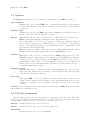
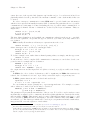
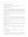
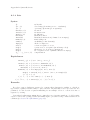
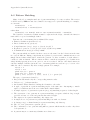
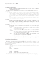
1.4.1 Multiplexed buffer example
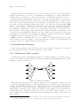
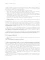
Consider the problem of transmitting a number of message streams over a single data connection. We can share a single channel between the streams by adding multiplexing and demultiplexing processes, as in figure 1.
Ti
Ri
SM
RM
Figure 1: Multiplexed Buffers
This solution is inadequate if we wish to synchronise the sending and receiving processes
because the multiplexing introduces additional buffering into the channel. Typical specifications
on such a system might include the need to ensure that one lane does not interfere with another,
and that there is a bound on the amount of buffering introduced by the network. We therefore
insist that the connection between each sender and the corresponding receiver acts as if it were
a simple single place buffer like COPY (see Section 1.3.2 [Simple buffer example], page 7).
The combination of N channels then behaves like the unsynchronised parallel composition of N
simple buffers.
3
Mathematically, the abstraction function into the denotational model combines the information from the set
of all states reachable on a given trace to determine the corresponding observable behaviour.
Chapter 1: Introduction
9
COPYj = leftj ?x → rightj !x → COPYj
SPEC =
COPYi
i∈1..N
Our requirement on the multiplexed system is that it refines this SPEC process. To avoid
the introduction of extra buffering and interaction where one channel clogs the system when its
receiver does not pick up messages soon enough, we introduce acknowledgement signals from
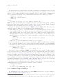
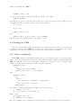
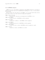
the receivers to the senders as in the earlier example. This can also be multiplexed through a
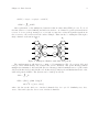
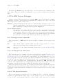
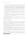
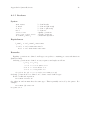
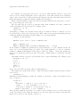
single channel, as shown in figure 2.
Ti
Ri
SM
RM
RA
SA
Figure 2: Multiplexed Buffers with Acknowledgement
The implementation will therefore consist of N transmitters (Ti ), N receivers (Ri ) and
four processes which manage the forward and reverse channels: SM (Send Message) which
multiplexes transmitted data and RM (Receive Message) which demultiplexes it, together with
SA (Send Acknowledge) and RA (Receive Acknowledge) which perform similar functions for the
acknowledgement channel. The system can be built up as follows:
INS =
Ti
i∈1..N
LHS = (INS k (SM
X
RA))\X
where X = {|mux , admx |}
where left denotes the whole set of indexed channels lefti , for i ∈ 1..N . Similarly mux , dmx ,
amux , admx and right also denote sets of indexed channels.
Chapter 1: Introduction
OUTS =
10
Ri
i∈1..N
RHS = (OUTS k (RM
Y
SA))\Y
where Y = {|dmx , amux |}
SYSTEM = (LHS k RHS )\Z
Z
where Z = {|mess, ack |}
If this implementation is correct, then we will have
SPEC v SYSTEM
Establishing this using traces refinement shows that the multiplexed buffers perform no
incorrect events. Using failures-divergence refinement will show that they cannot diverge, and
cannot refuse input on any of the individual channels which is empty nor refuse output an any
channel which is full. Failures refinement alone could show that the buffers never get into a
stable state that can refuse a set not permitted by the specification, but would not exclude
divergence — which obviously looks like refusal from the outside.
This example is explored further in the tutorial (see Chapter 3 [Tutorial], page 20), and a
listing of the FDR2-compatible source can be found in Appendix E [Multiplexed Buffer Script],
page 77.
Chapter 2: Using FDR
11
2 Using FDR
This chapter describes the basic structure and interface of the FDR tool. The FDR graphical
user interface is based on John Ousterhout’s Tcl and Tk toolkits. It is designed to be familiar
to users of Motif, SAA, or Microsoft Windows style applications1 .
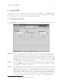
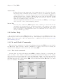
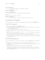
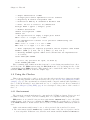
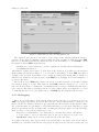
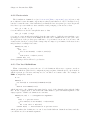
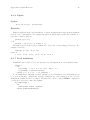
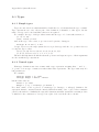
2.1 The Main Window
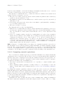
When FDR is started, it displays a window of the form shown in Figure 3. This is made up
of five components arranged vertically.
Figure 3: Main Window
Menu Bar At the top of the window, the menu bar includes headings describing groups of
related commands. To pop up the menu related to a heading, click with Mouse-1
(usually the left mouse button). Alternatively, hold down the Alt (or Meta) key and
type the character which is underlined in the heading. This area also includes the
Interrupt button which stops the current check or compilation and prepares FDR
to act immediately on further commands.
Tab Bar
The second portion of the window is a strip containing tabs for the different kinds of
checks that FDR can perform. There is also a tab for interaction with the compiler
and evaluation of arbitrary expressions.
Tab Pane
The middle part of the main window is used enter information relevant to the currently selected tab. This can be for building up refinement statements or for evaluating expressions. In the case of a simple refinement, two process selectors define the
specification and implementation rôles in the check, and the type of refinement relation can also be varied. (Of course, for deadlock, livelock and determinism checks
only one process needs to be selected, and this area contains a single selector.) Once
selected, a check can be added to the list of assertions or checked immediately.
1
Although it is not formally compliant with these standards.
Chapter 2: Using FDR
12
Assertion List
Perhaps the most important part of the main window lies below the tab pane:
the assertion list contains the assertions made about process refinement, deadlockor livelock-freedom, or other model properties. For each statement, FDR shows
whether it is true, false, or untested. When a file is loaded, the assertion list contains
any refinement properties stated in the script file. Properties are added to this list
when the an enquiry is made by the user.
Assertions displayed in this list can be tested, and if false, the FDR process debugger
can be invoked on the counterexamples generated.
Process List
Below the list of assertions, FDR displays a list of all the processes defined in the
currently loaded script (and also any functions which could return process results
if provided with suitable arguments). Processes selected from this list can be used
as the specification or implementation parts of a refinement check, or tested for a
variety of intrinsic properties.
2.2 On-line Help
To obtain information about FDR while the tool is running, select the Help menu from the
right-hand end of the menu bar (using Mouse-1). This displays a hypertext version of this
manual. The browser used to show the manual can be configured as described in Section 3.2.1
[Environment], page 23.
2.3 File and Model Commands
The most basic commands for loading and analysing systems using FDR are grouped under
the File menu. This currently contains commands for loading a new model, re-loading the
current model, editing the current source file, and exiting FDR.
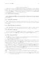
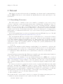
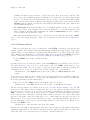
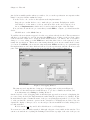
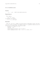
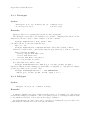
2.3.1 The Load command
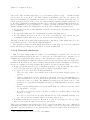
Selecting this option from the menu causes FDR to display a dialogue box requesting the
name of a file to load. This box will have the general form shown in Figure 4. To change
directories, select the appropriate directory in the right-hand column or type into the entry area
displayed above it; to select a file choose it from the left-hand column, or type its name into the
left-hand entry area. To load a file into FDR, select it and then click the OK button; to cancel
the load command, click Cancel.
Chapter 2: Using FDR
13
Figure 4: File Selection Window
When a file is loaded, any existing assertions and process definitions are cleared, and the
assertion and process lists are initialised with those defined in the script file (and those included
from the script file). Should syntax or other errors occur when loading a file, error messages will
be appended to FDR’s log of internal activity. This can be displayed by selecting Show Status
from the Options menu (see Section 2.7 [Options], page 16).
2.3.2 The Reload command
This command causes FDR to re-read the file which is currently loaded, incorporating any
changes which may have been made since the file was last read. If no file is loaded, this command
is not available.
2.3.3 The Edit command
This command presents the currently loaded file in an editor. The editor used can be configured, as described in Section 3.2.1 [Environment], page 23. If no file is loaded, this command
is not available.
2.3.4 The All Asserts command
This command runs all the assertions in the assertion list for which no result is currently
known. It can be used to perform checks in bulk, for regression testing or other purposes.
2.3.5 The Exit command
When this command is selected, FDR displays a dialogue box asking the user to confirm that
they wish to kill the current FDR session. If the response is Quit then FDR terminates.
2.4 The Assertion List
An FDR CSP script file can include statements making assertions about refinement properties. These statements will typically have the following form
assert Abstract [X= Concrete
where Abstract and Concrete are processes, and ‘X’ indicates the type of comparison: ‘T’ for
traces, ‘F’ for failures, or ‘FD’ for failures-divergences. When such a script file is loaded, any
assertions of this form are listed in the FDR main window. Initially, each such assertion is
marked as unexplored, using a question mark symbol.
An assertion can be selected by clicking on it with Mouse-1. The currently selected assertion
can be submitted for testing by choosing the Run option from the Assert menu. FDR will then
attempt to prove the conjecture by compiling, normalising and checking the refinement (see
Section 1.2 [The CSP View of the World], page 3). While a test is in progress, the assertion will
be marked with a clock symbol, to indicate that FDR is busy.
When a test finishes or is stopped by the interrupt button, the symbol associated with the
assertion will be updated to reflect the result:
Tick
indicates that the check completed successfully; the stated refinement holds.
Cross
indicates that the check completed, but found one or more counterexamples to the
stated property: the refinement does not hold, and the FDR debugger can be used
to explore the reasons why.
Chapter 2: Using FDR
14
Exclamation mark
indicates that the check failed to complete for some reason: either a syntax or type
error was detected in the scripts, some resource was exhausted while trying to run
the check, or the check was interrupted. If a process could not be compiled, FDR
will also indicate this by popping up a warning dialogue box. Other error messages,
and further information, are available in the status log (see Section 2.7 [Options],
page 16).
Zig-zag
indicates that FDR was unable to complete a check because of a weakness in the currently coded algorithms. (This can occur under rare cirumstances when performing
a determinism check in the Failures model.)
When a check has been completed, either a tick or cross will be displayed. If this symbol
has a small dot next to it, then counter-examples are available and the check may be sensibly
debugged.
The FDR debugger can be invoked on the result by double-clicking on it, or by selecting the
assertion and choosing Debug from the Assert menu. This will open a new window allowing the
behaviour of the processes involved to be examined. The FDR process debugger is described
in detail below (see Section 2.9 [The FDR Process Debugger], page 17). An assertion can be
re-checked after termination (with different options, for example) by selecting the Run command
from the same menu.
Alternatively, assertions can be run or debugged using a pop-up menu which is invoked by
clicking on the assertion with Mouse-3 (usually the right mouse button).
In addition to the conjectures made about process refinements in the CSP script, the assertion
list will also record other postulates made by the user in the course of an FDR session using the
buttons in a tab pane (see Section 2.6 [The Tab Pane], page 15).
(It is possible to debug an assertion which does not display the small blob, but it is not productive since the underlying check was successful and the behaviour of none of the components
is relevant.)
2.5 The Process List
The list of processes which is displayed by FDR when a file is loaded serves two main purposes:
it allows the user to select processes for insertion into a tab pane, and it also allows the user to
invoke a variety of tests on intrinsic properties of processes.
The entries in the list consist of the name of each process or function which way return a
process, followed by the number of arguments required by the function, if any.
Selection in this window follows the same pattern as in the assertion list: Mouse-1 selects
the current process, and Mouse-3 invokes a pop-up menu of commands which can be activated
on the process under the cursor. The currently selected process may be transferred to the tab
pane by clicking one of the arrow buttons, or used in any of the following commands from the
Process menu:
Deadlock
Tests to determine whether the process can reach a state in which no further action
is possible. If a deadlock can occur, a trace leading to deadlock will be available to
the debugger.
Livelock
Tests to determine if a process can reach a series of states in which endless internal action is possible without any external events taking place (CSP divergence or
internal chatter). If such a sequence is found, it will again be accessible through
the debugger (which will allow examination of the details of the internal actions
involved).
Chapter 2: Using FDR
15
Deterministic
This command tests to determine if the process is deterministic; i.e., if the set of
actions possible at any stage is always uniquely determined by the previous history
of visible actions. A process will fail to be deterministic in this CSP sense if either
it can diverge (livelock), or if it is possible for a given action to be allowed after
a given trace of visible events and also possible that it could be refused after the
same trace. In this latter case, the debugger will present two behaviours of the same
process as a counterexample; one leading to the possible event, and one leading to
its refusal.
Graph
This option is currently experimental and available only if the environment variable FDRGRAPH is set. It produces a graph of the selected process which can be
manipulated (states can be rearranged) and printed.
2.6 The Tab Pane
The middle portion of the FDR main window allows the user to assemble and check properties
of processes defined by the model without adding explicit assertions to the file2 .
For each possible check, it consists of a number of components: selectors allowing processes
to be chosen; a selector for the CSP refinement relation (i.e., the semantic model used), and a
set of buttons for managing these assertions.
The process selectors operate identically: each consists of a title and three elements: a
selection button (the arrow symbol), a text field and a pull-down list. Each of these may be
used to modify the process definition displayed in the text field:
• Clicking on the selection button (the arrow symbol) causes the text entry to be set to the
process, if any, currently selected in the process list described in the previous section.
• Clicking on the text field enables standard text editing keys to be used to enter or modify
the text.
• Clicking on the pull-down button and selecting a process from the list which is then displayed
causes the text entry to be set to that value.
Additionally, these the text entries can be emptied by clicking the Clear button at the bottom
of the process selector.
The semantic model to be used for a check can be changed by clicking Mouse-1 on the Model
button of the tab pane; FDR2 will display a list of alternative models which can be selected with
Mouse-1. The choice of models may be constrained by the check under construction: deadlock
and determinism checks cannot be performed in the traces model, and divergence checks must
be performed in the failures-divergences model.
Three command buttons complete the tab pane. These allow checks to be recorded and
tested as follows:
Check
The check is added to the assertion list and immediately run.
Add
This causes a check to be added to the assertion list as above, but the check is not
immediately started; it may be run later using any of the mechanisms described
above (see Section 2.4 [The Assertion List], page 13).
Clear
Clicking this button clears any process selectors, ready for a new definition to be
selected or typed.
2
It thus provides the same user interface function as the FDR1 interface.
Chapter 2: Using FDR
16
2.7 Options
The Options menu allows access to a number of internal aspects of FDR’s operation.
Supercompilation
Clicking this option toggles FDR’s use of an internal mask-based representation
for finite-state machine compositions. It should be left enabled for all standard
operations.
Bisimulate leaves
Clicking this option toggles FDR’s automatic bisimulation of all leaf processes. It
should be left enabled for all standard operations.
Messages
This submenu allows control of the amount of feedback added to the status log by
FDR’s internal state-machine manipulation and testing functions.
The default, Auto, does not report operations covering fewer than two hundred
states, indicates progress every hundred states to two thousand, every thousand
states to four hundred thousand, every ten thousand states to eighty million, and
every hundred thousand thereafter.
Full verbosity gives details of all such operations; None inhibits all such status
information. To view this log information, use the Show Status option.
Compaction
This allows control over the compaction used on FDR’s main data storage. The
Normal setting is recommended for most examples. Selecting Off will approximately
double the storage consumed during a check. High decreases the storage used by
approximately a third, at the cost of increasing the amount of processor time taken
(this is useful for problems which might otherwise exceed the available storage, or
on machines with fast processors).
Examples per check
This allows the user to control how many counterexamples may be generated by a
single check. By default at most one may be generated. (This option was previously
controlled from the status window.)
Show status
This causes FDR to open a scrollable text window which will be updated as it
carries out the compilation and checking processes. This status window also receives
detailed error messages describing syntax or semantic errors detected by the CSP
compiler.
A Restart option is displayed on the options menu of some releases of FDR. At the present time
this is intended for internal use only.
2.8 Tab Bar Commands
The following buttons on the tab bar select the relevant page in the tab pane. From this
page the user can invoke commands which operate on a selected process, as described under the
corresponding command (see Section 2.5 [The Process List], page 14).
Deadlock
Checks the selected process for deadlock.
Livelock
Checks the selected process for divergence (livelock).
Determinism
Checks the selected process for determinism.
Chapter 2: Using FDR
17
In addition, the Evaluate page allows the user to enter an expression for evaluation by the
CSP compiler. This can be useful for checking the correct operation of functions used within a
script.
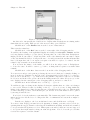
2.9 The FDR Process Debugger
When a completed check is selected for debugging, FDR creates a new window containing
information about the counterexamples (if any) which were found in the course of the check.
This debugger view consists of three areas:
Menu Bar As in the main window, the menu bar contains headings describing groups of commands for manipulating or querying the debugger. At present these headings include
File commands (for closing the window), and the Help menu.
Process Behaviour Viewer
The largest portion of the debugger view is devoted to this display, which shows
the structure of a particular process together with its contribution to a particular
counterexample. Where more than one process or rôle are involved in a check (e.g.,
in a comparison between a specification and an implementation), the individual
processes can be selected by the “file tabs” across the top of this region.
2.9.1 Debugger menu commands
The current release of FDR supports only a few simple commands on the debugger view
menu bar:
File
This contains a Close command, which causes the debugger window to be closed.
(The save option is intended for testing purposes only.)
Help
Gives access to the on-line help facility described (see Section 2.2 [On-line Help],
page 12).
2.9.2 Viewing process behaviours
The behaviour viewer is organised as a series of pages indexed by numbered tabs, one for
each process relevant to the currently selected counterexample (see Figure 6 in Section 3.2.3
[Debugging], page 25). For any particular counterexample, the system maintains a record of
the processes involved. If the property being checked was intrinsic, like deadlock- or livelockfreedom, there is only a single process involved. In the case of a refinement check, there will
be two processes, a specification and an implementation. In this case, FDR will display the
behaviour of the implementation by default (labelled with tab 1), but we can choose to view
information about the specification by clicking the alternative “file tab” (labelled 0).
Each page thus represents a single process and its involvement in a particular behaviour.
This information is represented in two parts: a hierarchical view of the structure of the process,
and a series of windows showing the contribution of a selected part of the process to the overall
behaviour.
2.9.2.1 The process structure
The process structure is represented as a tree similar in form to a standard organisation
diagram or program structure chart. The root node (at the top of the tree) represents the
process as a whole, and is initially shown alone, with no further detail. Any leaf node for which
Chapter 2: Using FDR
18
more information is available can be expanded by double-clicking with Mouse-1; double-clicking
a node which is currently expanded will cause that part of the tree to be “folded up”.
When a leaf node is expanded, branches are added according to the number of subcomponents of the node in question. Thus, a node labelled with a parallel composition symbol
‘[|..|]’ will expand to have two children representing the sub-processes which are combined
in parallel. Each child will be associated with its own contribution to the overall erroneous
behaviour being examined3 .
If any of the compression or factorisation operators (see Section 5.1 [Using Compressions],
page 34) were applied in building up a system, the process of extracting the back-trace information may involve further refinement checks and thus significant computation. To indicate this,
nodes of the process structure corresponding to compressed processes will be coloured red, and
will not be expanded by default. Examining their internal behaviour is still straightforward,
however: simply double click on the coloured node.
(Note: some lesser-used CSP constructions, such has the repetition operator ∗ of [Hoare85],
have a single syntactic sub-component which may be responsible for more than one independent sub-behaviour. In this case, the process tree will contain a branch for each independent
behaviour. There are currently no operators which involve both multiple processes and multiple
behaviours!)
2.9.2.2 The behaviour information
When exploring the process structure view, any node in the tree can be selected by a single
click with Mouse-1. Information about the currently selected node is displayed in the area to
the right of the window. The exact information displayed will depend on the nature of the
counterexample being examined and the contribution made to it by the selected component. In
general, the following types of information may be displayed:
• An erroneous trace, ending in a prohibited event. This will be flagged Allows, and will be
displayed as a scrollable list. By default, internal actions (τ events) will be included, but
these can be hidden by toggling the Show tau option button displayed at the bottom of the
list.
• A non-erroneous trace, perhaps leading to an error elsewhere but not in itself illegal. This
will be labelled Performs, and can be manipulated as for an erroneous trace.
• An illegal acceptance or refusal. This information can be expressed either as an acceptance
set (which will be smaller than the specification permits) or as a refusal larger than any
legal maximum. To switch between these views, click on the Acc. (acceptances) or Ref.
(refusals) button displayed below the set. In some cases, information will be available on
which behaviours the specification was willing to permit. To display this, click on the
Allowed. . . button; the information will be displayed in a pop-up window.
• Divergence. If a process diverges illegally, this will be stated.
• Repetition of visible events. In the course of decomposing a divergent behaviour (e.g.,
through a hiding operator), we may discover a series of visible events which can be repeated
endlessly, and which are all concealed from the ultimate environment. This sequence will
be labelled with the word Repeats and will be displayed in the same manner as the other
traces discussed above.
Typically the following information will be displayed for each type of counterexample behaviour:
3
Occasionally, process constructs may arise in which a single syntactic subcomponent has more than one
independent contribution to the behaviour being examined. In this case one branch will be created for each
contribution.
Chapter 2: Using FDR
19
Successful refinement
(or no relevant behaviour): no information displayed.
No direct contribution
a non-erroneous trace.
Refusal/acceptance failure
a non-erroneous trace, plus the illegal refusal/acceptance.
Divergence
the trace leading to divergence.
Divergence (internally)
the trace leading to divergence, plus a trace of repeated events.
2.10 Interface Conventions
The following sections document the (fairly standard) conventions used in the FDR interface.
2.10.1 GUI conventions
These general rules apply to the FDR user interface:
• Single-click with Mouse-1 (usually the left mouse button) selects activates a menu or button,
or selects an item from a list.
• Double-click with Mouse-1 invokes an action on an object.
• Mouse-3 (usually the right mouse button) invokes a pop-up menu for the object under the
cursor.
• Check boxes have square indicators and can be “on” or “off.” The option is off when the
box is the same as the background colour, and on when it is otherwise lit.
• Radio buttons are used in a group, and are like a collection of check boxes, except they
have diamond shaped indicators and only one option from the group can be selected (or
“on”) at any time.
2.10.2 Keyboard short-cuts
Keyboard input can be used for the vast majority of input to FDR. The general guidelines
are:
• Clicking on an object with the mouse directs subsequent input to that object.
• Pressing the Tab key moves input to the next item; pressing Shift-Tab moves input to the
previous item.
• The Enter (or Return) key invokes the item currently accepting input.
• Pressing the Alt key with a letter raises the menu identified by that letter. Items can be
selected from a menu using the letter underlined in the item title. Press the Esc key to
cancel a pop-up menu.
Chapter 3: Tutorial
20
3 Tutorial
This chapter presents a short tutorial on formulating a specification and creating implementations. FDR is then used to show whether the implementation is valid, with respect to the
specification.
3.1 Describing Processes
The CSP notation, of which we have seen a number of examples so far, developed as a
collection of algebraic operators denoting various ways of building and combining processes. To
apply an automated tool to CSP definitions we need a way of entering them into computers:
CSP needs to become more like a programming language. The most important decisions that
have to be taken in doing this are not so much how to represent the operators in machinereadable form, but less obvious issues such as the collection of data-types to be supported for
values passed over channels and as the state of processes, and the way a program and definitions
are structured.
A proposed standard has been developed at Oxford under an ONR-funded project. The full
language is described in Appendix A [Syntax Reference], page 43.
The only significant difference from the version of CSP in Hoare’s book is in the treatment
of alphabets and how these affect parallel composition. In the modern treatment, processes
do not have intrinsic alphabets as in Hoare’s book. This requires us to specify the interface
between processes operating in parallel explicitly. Rather than the single synchronised parallel
composition operator (P k Q) used by Hoare, we employ an operator parameterised by the
interface sets of the components: in
P X kY Q
(expressed in the machine-readable language as P[X||Y]Q), P is constrained to perform only
events in X , Q performs events from Y , and events in the intersection X ∩ Y are synchronised.
A useful alternative is to specify a set of synchronised events and allow events outside this set
to be interleaved. Where this interface set of synchronised events is X , we write this as
P k Q
X
(expressed in linear form as P[|X|]Q). This form of parallel composition makes many definitions
more concise, and is the one generally used in the example files.
The reference to the language of process definitions interpreted by FDR can be found in
Appendix A [Syntax Reference], page 43. The remainder of this section describes the practical
usage of the language. Larger examples of how the syntax works, and of various styles that
can be useful in designing CSP processes, may be found in the supplied examples in the ‘demo’
directory.
Processes are described by giving the checker a series of equational definitions, in the usual
CSP style. An input file to FDR may consist of a series of such definitions, plus additional
information about the environment in which the definitions should be interpreted. To assist in
making descriptions comprehensible, comments may be included: a double-dash (‘--’) and any
subsequent text on the line are ignored if they occur in either of the following positions:
• after a definition (or before the first definition in a file)
• after a binary operator
Line breaks can also occur at either of the above positions. To facilitate structuring and re-use
of definitions, system descriptions can be split across files. The command
include "myfile.csp"
Chapter 3: Tutorial
21
causes the text of the specified file (‘myfile.csp’ in this case) to be read in as if it had been
physically included at the point where the include command occurs. Such included files can
be nested.
In order to interpret communication events, FDR must be provided with some information
which is often expressed informally in written CSP documents. In particular, the set of possible
communications events must be defined, including the sets of possible values communicated on
each referenced channel. Events or channels are declared by the keyword channel. Thus, we
might write:
channel c1,c2 : {v1,v2,v3,v4}
V = {v1,v2,v3,v4}
channel d1,d2 : V
The first defines channels c1 and c2 which can communicate values from the set v1. . . v4, while
the second is equivalent, except that the type is described by a name, previously defined as a
set of values.
FDR actually allows almost1 arbitrary set expressions after the colon:
channel decrease : { i.j | i<-{1,2,3}, j<-{1,2} }
Other data-types can be declared by a datatype clause:
datatype V = v1 | v2 | v3 | v4
channel c1,c2 : {v1,v2,v3,v4}
channel d1,d2 : V
To declare a simple event, rather than a channel passing values, we simply omit the type term:
channel e1,e2,e3
To allow the use of more complex CSP communication constructs, we can declare dotted compound events, for example after a declaration
NUMBERS = {0,1,2,3}
datatype X = a | b | c | d
channel xxx : NUMBERS . {a,b,c}
the output xxx.1!b and the input xxx.i?v (where i is in {0,1,2,3}) are valid event descriptions.
In FDR1, the order of these declarations could be significant; in FDR2 this restriction is
relaxed, but “declaration before use” is probably a reasonable style to adopt in any case.
In FDR, genuine functions can be declared and used freely:
square(n) = n * n
P = in ? x -> out ! square(x) -> P
Process definitions can use parameters to represent internal state. For example, a counter
whose values are bounded by 0 and N may be described:2
COUNT(n) = n!=0 & down -> COUNT(n-1)
[] n!=N & up -> COUNT(n+1)
The parameter n represents the internal state of the process. To be able to explore such processes
mechanically, we must be able to enumerate their states (although this is not strictly true in the
full generality of FDR). Thus an unbounded counter, which has an infinite state space, could
not be checked by FDR, and indeed attempting to use such a definition may cause FDR to enter
an endless loop3 . The data-types which can be used as process parameters include truth values,
integers and also sets and sequences of such values.
1
2
3
The resulting set must actually be rectangular (see Section A.3.3 [Datatypes], page 53).
Of course, this COUNT (n) is a finite process only if n is between 0 and N . . .
Again, this is not strictly true, as FDR has the capability to check refinements involving some kinds of infinite
processes. In particular, infinite specifications such as “is a buffer” have been used experimentally in FDR,
but the compiler does not yet support such features.
Chapter 3: Tutorial
22
Because interfaces are usually defined in terms of channels, not individual events, a special
notation is provided for writing event sets: the notation {|a,b,c|} expands to a set of events
when a, b, c are either individual events or channels. The set of all possible communications
along a channel is substituted for the channel name in the latter case. Thus, if we declare
channel a : {0,1,2}
channel b : {open, close}
channel d
we have
{| a,b,d |} == {a.0, a.1, a.2, b.open, b.close, d}
FDR also supports unsynchronised parallel composition (P|||Q), hiding (P\A), renaming
(P[[a<-b]]) and ‘linked parallel’ (P[out<->in]Q). These operators and the manner in which
they may be used are discussed in Section A.4 [Processes], page 56.
Any process structure which is allowed in FDR1 is valid in FDR2. The latter, however,
relaxes the former’s "high/low level" distinction in two significant ways:
• When high-level operators occur in the definition of a (parametrised) process, the dependency graph is checked to see whether the given process/parameter combination is (apparently) required in its own evolution. If not, then the compiler generates a high-level tree
(including high-level forms of prefixing and choice, if necessary) for the checking process.
This allows the use of parameters to define regular finite compositions of processes: thus
channel a
P(n) = if n == 0 then a -> STOP else P(n-1) ||| P(n-1)
Q = P(10)
defines Q to be a process which can do 1024 a’s before stopping.4
• In the case that the process does depend on itself, the compiler can fall back on evaluating
the operational semantics of the operator itself. Frequently, this will be a nonterminating
calculation; but there are some useful idioms which benefit from this possibility, particularly
in conjunction with sequencing:
channel a,b,c,d,e
P = (a -> b -> SKIP ||| c -> d -> SKIP); e -> P
One form of operator available in FDR2, but additional to those offered by earlier versions,
is the transparent function. These are typically used for compression functions, such as those
described in Section 5.1 [Using Compressions], page 34. According to the philosophy of [Scat98],
their gross semantic effect should be that of the identity function, since any tool which does not
recognise them is entitled to ignore them; but they may dramatically affect the way in which
those semantics are realised operationally. The range of functions supported in this way is
determined at link-time of the refinement engine, and thus may be extended; those currently
supported are described in Section 5.1 [Using Compressions], page 34.
In order to use a transparent function, it must be made known to the parser using the
transparent keyword, and may then be applied to any process term:
transparent diamond
... etc ...
P = Q [| A |] diamond((R [| B |] S) \ B)
3.1.1 Sample script for FDR2
We will illustrate some of the points above in an FDR2 version of the one place buffer (see
Section 1.3.2 [Simple buffer example], page 7).
4
And which incidentally has 21024 states, which it would not be wise to try and explore directly; applying a
compression such as normalise to the “else” branch makes such constructs entirely reasonable, however.
Chapter 3: Tutorial
-----
23
Simple demonstration of FDR2
A single place buffer implemented over two channels
Original by D.Jackson 22 September 1992
Modified for FDR2 by M. Goldsmith 6 December 1995
-- First, the set of values to be communicated
datatype FRUIT = apples | oranges | pears
-- Channel declarations
channel left,right,mid : FRUIT
channel ack
-- The specification is simply a single place buffer
COPY = left ? x -> right ! x -> COPY
-- The implementation consists of two processes communicating over
-- mid and ack
SEND = left ? x -> mid ! x -> ack -> SEND
REC = mid ? x -> right ! x -> ack -> REC
-- These components are composed in parallel and the internal comms hidden
SYSTEM = (SEND [| {| mid, ack |} |] REC) \ {| mid, ack |}
-- Checking "SYSTEM" against "COPY" will confirm that the implementation
-- is correct.
assert COPY [FD= SYSTEM
-- In fact, the processes are equal, as shown by
assert SYSTEM [FD= COPY
Files containing CSP definitions in this form can be created using any standard text editor,
and loaded into the FDR2 system using the File|Load menu or by specifying the file on the
command line when FDR2 is started. This example can be found in the ‘demo’ directory of the
standard FDR2 distribution, in the file ‘simple.csp’.
3.2 Using the Checker
This section is intended to guide you, the user, through a typical series of interactions with
the tool, exploring variants of the system described above (see Section 1.4.1 [Multiplexed buffer
example], page 8). The experiments are relatively small, compared with the full capabilities of
the tool, and should take no more than an hour or so to complete in total. It is recommended
that you see Chapter 2 [Using FDR], page 11 for a description of the position of the controls of
the tool.
3.2.1 Environment
The system is currently implemented to run under the X Window System, Version 11, and
you must be using a console or monitor running X11 or a compatible windowing system.
FDR insists on one variable being set in its environment: FDRHOME must be set to the (fully
qualified) name of the directory containing the FDR ‘LICENCE’ file, typically the root directory
of the FDR installation. If this variable is not set, the tool will terminate immediately with an
error.
Other environment variables may be set, to select preferred editors and web browsers.
• The environment variable FDREDIT may contain the name of the editor you prefer to invoke
to view script files. If this is not set, then the environment variables VISUAL and EDITOR are
Chapter 3: Tutorial
24
examined (in that order) and if none of these is set the editor vi is selected. In all of the
above cases, an X terminal application is launched to host the editor (so the program xterm
needs to be found along your search path); if your chosen editor opens its own X-window (like
xedit and modern versions of Emacs), then supply its name in the environment variable
FDRXEDIT instead, which overrides the other variables and launches the editor without the
extra terminal application.
• The FDRBROWSER environment variable, if set, determines which browser to use to view the
hypertext version of the manual. The browser is assumed to be an X11 application and
will be launched directly, rather than inside an xterm. If FDRBROWSER is not set, a simple
browser written in Tcl/Tk will be used.
Other environment variables allow you to control the location of various components of FDR,
and to control its paging strategies. These are documented in Appendix D [Configuration],
page 75.
3.2.2 Getting started
This section should help to give you a first taste of using FDR, by leading you slowly through
a simple example. The example deals with multiplexing of multiple streams of data down a single
channel, using a second channel for returning acknowledgements. You will need the CSP script
called ‘mbuff.csp’, which may be found in the ‘demo’ directory supplied with FDR. (A printed
version of that script can found in Appendix E [Multiplexed Buffer Script], page 77.)
To invoke FDR2, type at the command prompt
fdr2
and wait a short period for the appearance of the main FDR window (see Figure 3 in Section 2.1
[The Main Window], page 11). It is often useful to also have FDR’s status window open,
especially when trying out a new script, because the status window will show parsing and
compilation errors. You won’t really need it for this example, but open it anyway:
Click Mouse-1 on the Options button, move the pointer over Show status and click
again.
You now have two windows. Move them around by dragging their title bars until you find nice
positions for them; if they have to overlap, have the main window to the front. You will make
most subsequent input via the main window.
Next we need to have FDR load the script ‘mbuff.csp’. To do this
Click Mouse-1 on the File button, move the pointer over Load and click again.
The file selection window (see Figure 4 in Section 2.3.1 [The Load command], page 12) will
then appear. The window has two main areas, the one to the right for moving up and down
the directory tree, and the one to the left for selecting a particular file. If, when you invoked
FDR, you had the correct current directory then you will see the file name ‘mbuff.csp’ listed
in the left-hand area, although to make the name visible you may need to drag a slider that
appears to the right of that area when there are too many names for the space provided. If
‘mbuff.csp’ does not appear in the list then you can go searching through the directory tree
(for the ‘demo/misc’ directory) by double-clicking Mouse-1 on the folder icons. When you’ve
found it, have FDR load it:
Click Mouse-1 on the file name, and then click on Ok.
The file selection window will disappear, and after a short delay new information will appear
within the main window: an assertion will appear in the Assertion List (just below the Tab
Pane) and a list of processes in the area below that, exactly as in Figure 5.
Chapter 3: Tutorial
25
Figure 5: Main Window after Loading mbuff.csp
The assertion was chosen by the writer of the script as the natural refinement check to
perform. Notice there is currently a question mark (?) symbol against it. This is because FDR
has not yet established whether the assertion holds, so the next thing to do is ask FDR to check
the assertion; this is FDR’s main function:
Click Mouse-3 on the assertion, to produce a small action menu, and from this menu
select Run with Mouse-1.
Alternatively, a faster way is just to double-click on the assertion. You will notice the question
mark against the assertion change to a clock symbol, informing you that FDR has started
working on the problem. You will also notice output appearing in the status window, which you
will find very useful as you gain experience with FDR; for now simply view it as reassurance of
progress being made.
After a short period FDR will complete the check. You will notice the clock symbol against
the assertion change to a tick. That tells you that FDR found the assertion to be correct, in
this case showing that a combination of transmitters and receivers communicating through a
pair of wires behaves like several independent one-place buffers. There is nothing more you can
do with this assertion: it doesn’t make sense to ask FDR why the implementation works. . .
3.2.3 Debugging
There is a broken version of the system defined in the same file; you can use it to try out
FDR’s debugging capabilities. For the broken version a corresponding assertion could have been
inserted in the file, which would have popped up with the other assertion in the Assertion List.
We would then have needed simply to select that and start a second check. But since no such
assertion appears in the file, we must build one using the Tab Pane (just below the Tab Bar).
First you need to select the specification process:
Drag the process-list slider so as to make the process name Spec visible, click Mouse1 on the name to select it, and then click on the arrow button below the word
Specification, which can be found towards the left of the Tab Pane.
You will see the name Spec appear in the text gadget just to the right of the arrow button.
Actually you could have clicked in the text gadget and typed in Spec directly, but the way you
Chapter 3: Tutorial
26
just did it is usually quicker unless you wish to choose as the specification an expression that
hasn’t been given a name within the script.
You also need to choose the broken system as the implementation:
Drag the process-list slider so as to make the process name FaultySystem visible,
click Mouse-1 on the name to select it, and then click on the arrow button below
the word Implementation, which can be found towards the right of the Tab Pane.
Now you have chosen the two processes that you wish FDR to compare, you should start the
check:
Click Mouse-1 on the Check button.
You will see the new assertion appear below the one you have already checked. The new assertion
will have a clock symbol to its left, showing that FDR is now working on the problem. After
a short wait and a little more output from the status window, you will see the clock symbol
change to a cross, telling you that FDR has found that this version of the system does not
satisfy the specification. This is more interesting than the previous, successful check because
you can now ask FDR to show why the refinement fails: FDR2 can show you a particular way
the implementation can behave that isn’t allowed by the specification, and also show how each
part of the implementation plays a part in producing the unacceptable behaviour.
Figure 6: Debugging Window
The first step in doing this is to bring up a debugging window (shown in Figure 6):
Click over the failed assertion with Mouse-3, to produce a small action menu, and
from this menu select Debug by clicking Mouse-1.
On the left side of the debugging window that has just appeared is an area for displaying the
processes being checked (the implementation rather than the specification, by default). At the
moment this area just contains the name of the process (FaultySystem) with a ‘\’ below it. The
‘\’ tells you that the outermost operator in the description of FaultySystem is hiding. You can
expand the display of this process to see the subprocesses from which it is built, arranged in a
tree-like structure:
Hold down the hCtrli key and double-click Mouse-1 over FaultySystem.
You can now see the tree fully expanded, although only part of it is visible in the window. You
can move around the tree by using the Panning Control in the top right of the view of the process
Chapter 3: Tutorial
27
tree. The larger, grey rectangle represents the entire area of the tree, whereas the smaller white
rectangle represents the displayed area. View the root of the tree:
Drag the white rectangle with Mouse-1 so that it is horizontally centred and as high
as possible within the grey rectangle.
You will see that the root is still selected (highlighted in blue), which assures you that the other
information in the debugging window applies to the process as a whole. That other information,
displayed in the central and right-hand areas of the debugging window, is the behaviour that
FDR has found to be exhibited by FaultySystem, although not by Spec.
In this case, it is a failure of liveness, which you can tell by the right-hand area having the
heading Accepts. Such a behaviour consists of a perfectly acceptable trace of events performed
by FaultySystem and an unacceptably small set of events that FaultySystem may then offer to
its environment. The trace is displayed in the central part of the debugging window, headed
Performs. Read it from top to bottom:
• The trace begins with the event left.t3.d 1; this represents the data item d 1 being taken as
input by the transmitter labelled t3.
• Next come three t au events. Strictly speaking, these are not part of the trace: they
are FDR’s way (and the generally accepted way within the literature) to display invisible changes of state; these particular t au’s are events performed by subprocesses of
FaultySystem that are obscured by a hiding operator.
• Next in the trace comes the event right.t3.d 1; this represents the data item d 1 being
produced as output, by the receiver labelled t3.
• Lastly there is one more t au event.
The t au’s can get in the way when there are many of them, in which case they can be removed
by clicking with Mouse-1 on the Show tau button, below the displayed trace. In this example it
is better to leave them visible.
Looking now at the right-hand area of the debugging window you can see a set of events that
FaultySystem may offer to its environment after performing the above trace. The display shows a
set containing left.t1 and left.t2. Actually both of these are channels rather than events; FDR’s
convention when displaying sets of events is to use a channel to represent the set of all events
that can be passed on that channel, so in this case the fully expanded set of events would have
members left.t1.d 1, left.t1.d 2, left.t2.d 1 and left.t2.d 2. The form displayed is more concise,
which is especially important when there are a lot of events in an acceptance.
You might not immediately see what is wrong with this set of events being offered, but you
can ask FDR to show you which sets Spec might offer after performing the same trace:
Click Mouse-1 on the Allowed... button, which is just below the area where the sets
of acceptances are displayed.
A new window (as shown in Figure 7) appears showing in its top half the set of events offered by
System, and in its bottom half the sets of events that Spec might offer. In this example, there is
no non-determinism in the behaviour of Spec and so there is only one set displayed in the bottom
half of the window, which Spec is therefore guaranteed to offer. Again notice the use of FDR’s
channel convention in displaying the set: what looks to be a single member left, actually stands
for all events passable by the channel left, which are left.t1.d 1, left.t1.d 2, left.t2.d 1, left.t2.d 2,
left.t3.d 1 and left.t3.d 2. In particular, notice that Spec is offering left.t3.d 1 and left.t3.d 2,
whereas FaultySystem is not. Now we can state precisely the nature of the failure: after passing
one data item between the transmitter and receiver labelled t3, that transmitter is not willing
to input a second value, although in the same circumstances Spec would.
Chapter 3: Tutorial
28
Figure 7: Acceptances Comparison Window
Another aid to interpreting the behaviour is to display what FaultySystem is refusing rather
than what it is accepting. First get rid of the most recently opened window:
Click Mouse-1 on the Dismiss button at the bottom of that window.
Then view the refusal set:
Click Mouse-1 on the Ref. button, at the bottom right of the debugging window.
You will see the heading of the right-hand display area change from Accepts to Refuses, and the
set being displayed change to {right, left.t3}, showing that out of all events that FaultySystem
might perform, it can refuse to output any value on the right channels, and can refuse to input
on the left channel labelled t3. Seeing as the trace of events performed shows that all items that
have been input have also been output, it is quite reasonable for right to be refused, but the
refusal of left.t3 stands out as an anomaly.
Now we know the nature of the failure, we will look at the subprocesses of FaultySystem
to locate the cause. It will be easier to go back to working with acceptance sets rather than
refusals:
Click Mouse-1 on the Acc. button at the bottom left of the debugging window.
You can view a subprocess’s part in producing the incorrect behaviour, by simply clicking on
its node in the tree (displayed to the left of the debugging window). Below the root of the tree
there is a node labelled ‘[|...|]’. This denotes the parallel composition of the two nodes that
lie below it, and is the next operator in from the hiding mentioned earlier. Keep an eye on the
trace displayed in the central part of the debugging window, and move to that node:
Click Mouse-1 in the left-hand area, over the ‘[|...|]’ node.
You will notice just one change in the displayed behaviour, which is that one of the t au’s changes
to mess.t3.d 1. This is because by clicking on the ‘[|...|]’ node you are looking within the
hiding of the channel mess, thus exposing the true event that gave rise to the t au. That in itself
doesn’t really help you here, but it should give you an idea of how information can be gained
by moving around the tree.
Now let’s look for the fault more systematically. The datum was passed between the transmitter and receiver labelled t3, so looking at the line of communication between those might be
a good start.
Pan the tree display to the bottom left-hand corner, and click Mouse-1 on Tx (t3).
You can see that Tx (t3) performs left.t3.d 1 (inputing a datum), performs sndm ess.t3.d 1 (requesting that the tagged datum be sent along the transmission medium), and is then determined
to accept an acknowledgement rcva ck .t3. This is quite reasonable behaviour: it is not supposed
to accept another input until receiving an acknowledgement. Now look at the process that
receives the request to send the datum.
Chapter 3: Tutorial
29
Click Mouse-1 on the node of the tree labelled SndMess.
You can see that SndMess performs sndm ess.t3.d 1 (receiving a request to send the tagged
datum), performs mess.t3.d 1 (the actual transmission of the datum), and is then ready to accept
the next request. Again, nothing wrong here: acknowledgements are not SndMess’s concern.
Now look at the process that picks up acknowledgements from the transmission medium — the
process that should have passed on an acknowledgement to Tx (t3).
Pan your view of the process tree slightly to the right (if necessary), so as to make
the node labelled RcvAck visible, and then click Mouse-1 over it.
Notice that RcvAck has not done anything (denoted by the trace list containing just the words
“Empty Trace”), although it is willing to accept an acknowledgement from the transmission
medium, just as it is supposed to. Thus, this process can not be blamed either. If you pan
to the very right of the tree you can check out the processes that lie at the other end of the
transmission medium, those labelled RcvMess and SndAck , but you will find correct behaviour
there also. This leaves just FaultyRx (t3) to check (and the name rather gives things away!).
Click Mouse-1 over the node labelled FaultyRx (t3).
You can see that FaultyRx (t3) performs rcvm ess.t3.d 1 (receiving an appropriately tagged datum
from the process RcvMess), performs right.t3.d 1 (sending the datum), and is then willing to
accept another tagged datum, but is not willing to produce an acknowledgement. This is the
cause of failure: it is necessary that FaultyRx (t3) sends an acknowledgement back through the
medium, to tell Tx (t3) it may input another datum.
This concludes the tutorial. You might feel that the example was slightly artificial, especially
as the subprocess we were looking for was clearly labelled Faulty, but in fact the way of working
we have just covered is very much what one does when using FDR on real design problems.
Often, of course, the systems are very much larger, sometimes with numbers of states running
into tens of millions, but often also the crux of a problem can be found with process descriptions
of the size shown in this example.
Chapter 4: Intermediate FDR
30
4 Intermediate FDR
This chapter aims to give some guidance in the use of FDR, falling between the introductory
chapters we have seen so far and the technical chapters which follow.
4.1 Building a Model
When approaching a new problem with FDR, it is tempting to dump a detailed description
of the problem into CSP as quickly as possible and “see how well FDR copes.” The results of
such an exercise are frequently disappointing. The model produced is usually intractable, and
ad-hoc attempts to simplify it tend to reduce its coherence and destroy any confidence in its
accuracy. Much better results are achieved by starting from a minimal model and incrementally
adding and testing features; in particular, incremental testing will reveal flaws soon after their
addition to the model.
Note that even if the initial model is small, the choice of identifiers and careful commenting
is still important. In particular, single character process and tag names are likely to cause
readability problems.
4.1.1 Abstract model
When adding detail to a simple model, it is only necessary to add those details which are
necessary to support the tests you intend to make. For example, the correctness of many
communication protocols is independent of the precise values being communicated and it may
suffice to replace the actual (large) space of values with a space of one or two values. (Although
such a simplification has intuitive appeal, the theory underlying it is still an active research
area.)
As well as simplifying the values communicated, it may be possible to omit some events
entirely and eliminate state from component processes. For example, the CSP vending machine
of [Hoare85] is given by
VM = coin -> choc -> VM
This discards almost all details including various coin sizes, the need to provide change and
the possibility that the machine may need refilling. Such abstraction may introduce nondeterminism, for example if we consider that the machine may become empty without modelling
the level, we obtain
VME = coin -> (VME |~| choc -> VME)
Nevertheless, such an abstraction can be useful. If we can show that VME satisifies some
specification then the same will be true for a more detailed model which does model the level,
such as
VML(n) = coin -> (if n>0 then choc->VML(n-1) else VML(0))
since
VME [= VML(N)
In extreme cases it may suffice to model a component with interface A as CHAOS(A), the most
non-deterministic divergence-free process with that interface.
4.1.2 Use components
For sound engineering reasons, complex systems are built out of simpler components with the
correctness of the system as a whole dependent on properties of the components, rather than on
precise implementation details. For properly designed systems, this structure can be exploited
to reduce the work involved in checking the system. For example, suppose we can write
Chapter 4: Intermediate FDR
31
SYSTEM = F(C_1, C_2)
for some components C_1 and C_2, and that we wish to check that
SPEC [= SYSTEM
and that the properties of the subcomponents can be expressed as S_1 and S_2. Then we can
establish the result we require by three simpler tests, namely
S_1 [= C_1
S_2 [= C_2
SPEC [= F(S_1, S_2)
since
SPEC [= F(S_1, S_2) [= F(C_1, C_2) = SYSTEM
follows by the compositional nature of the CSP operators.
4.2 Tuning for FDR
These sections discusses ways in which process descriptions can be tuned to get the best
from the current version of FDR. Since some of these features can be detrimental to the overall
readability of a script, they should be used with care and only when necessary.
4.2.1 Share components
When FDR builds state-machines from the CSP process descriptions, it does so as an acyclic
graph of process operators where the leaves of the graph are simple transition systems. Although
FDR can build the operator tree efficiently, construction of the leaves can be expensive. For
example, it is much more efficient to build an N -place buffer as
BUFF(N,in,out) =
let
COPY = in?x->out!x->COPY
within [out<->in] x : <1..N> @ COPY
than
BUFF(N,in,out) =
let
B(s) =
not null(s) & out!head(s) -> B(tail(s))
[]
#s < N & in?x -> B(s^<x>)
within B(<>)
and it is more efficient (assuming P and Q are both used) to write
P = BUFF(10, in, out)
Q = P [[ in<-left, out<-right ]]
than to write
P = BUFF(10, in, out)
Q = BUFF(10, left, right)
since the renaming can be built directly and the leaf process is then shared between P and Q.
Chapter 4: Intermediate FDR
¯
32
4.2.2 Factor state
The formulation of BUFF above (see Section 4.2.1 [Share components], page 31) is not only
more efficient because the COPY components are shared (and thus need only be calculated once),
but also because the state of the buffer has been distributed across separate processes. In general,
if we have a process P with two state variables x and y ranging over X and Y, so that
P(x, y) = f(P, x, y)
for some function f, and we can split the state so that
P(x, y) = Q(x) || R(y)
for some processes Q and R in parallel, then the time taken to build the state-machine corresponding to P can be reduced from #X*#Y in the first case to #X+#Y in the second. (Of course,
the exploration of the product space still has to be performed, but it can be done more efficiently as the check proceeds.) Such a change may not improve performance if the state is not
independent, for example if we write
BUFF(N,in,out) =
let
B(n, s) =
n>0 & out!head(s) -> B(n-1,tail(s))
[]
n<N & in?x -> B(n+1,s^<x>)
within B(0, <>)
then separating n and s will not be productive.
4.2.3 Use local definitions
When constructing processes, the use of local definitions allows us to separate out those
arguments which are passed in for configuration purposes (sizes, channels and so on) from those
which represent process state and may need to modified on recursive calls. For example, in
FDR1 we might have written
N = 6
BUFF(s) =
not null(s) & out!head(s)->BUFF(tail(s))
[]
#s<N & in?x->BUFF(s^<x>)
which ‘wires-in’ to the definition the name (and so type) of the channels along with the buffer
size. It also requires users to know that the buffer must be given an initial argument of the
empty sequence. With local definitons we can write
BUFF(N,in,out) = -- configuration arguments
let
B(s) = -- process state
not null(s) & out!head(s) -> B(tail(s))
[]
#s < N & in?x -> B(s^<x>)
within B(<>) -- initialisation of process state
which generalises the definition so it can be used with different channels and sizes and also
conceals the need for an initial argument.
Chapter 4: Intermediate FDR
33
4.3 Choice of Model
The hierarchy of models for CSP are useful because they provide differing amount of information about the processes, with a corresponding change in the cost of working in that model.
It is more efficient to perform a check in the simplest model which provides the required detail.
Property
Model
Safety
Traces
Liveness
Failures
Deadlock-freedom
Livelock-freedom
Failures-divergence
Note that the model_compress operation may produce better results in a simple process model.
Chapter 5: Advanced Topics
34
5 Advanced Topics
This chapter provides some more advanced material.
5.1 Using Compressions
This section outlines the currently available methods for compressing the state machine
representing a process, and gives some guidance in how and when to use them.
5.1.1 Methods of compression
FDR currently provides six different methods of taking a transition system (or state machine)
and attempting to compress it into a more efficient one. Each compression function must first
be declared by the transparent operator before it can be used (see Section A.6.2 [Transparent],
page 60). The functions must be spelt exactly as given below or the relevant operation will not
take place — in fact, since they are transparent, FDR will ignore an unknown function (i.e.,
treat it as the identity function) and simply give a warning in the status window (see Section 2.7
[Options], page 16).
explicate
Enumeration: by simply tabulating the transition system, rather than deducing
the operational semantics “on the fly”. This obviously cannot reduce the number
of nodes, but does allow them to be represented by small (integer) values, as opposed to a representation of their natural structure. This in turn makes subsequent
manipulations substantially faster.
sbisim
Strong, node-labelled, bisimulation: the standard notion enriched (as discussed in
[Roscoe94]) by the minimal acceptance and divergence labelling of the nodes. This
was used in FDR1 for the final stage of normalising specifications.
tau_loop_factor
τ -loop elimination: since a process may choose automatically to follow a τ action, it
follows that all the processes on a τ -loop (or, more properly, in a strongly connected
component under τ -reachability) are equivalent.
diamond
Diamond elimination: this carries out the node-compression discussed in the last
section systematically, so as to include as few nodes as possible in the output graph.
This is perhaps the most novel of the techniques, and the technical details are
discussed in Section 5.2.2.2 [Diamond elimination], page 40.
normalise
Normalisation: discussed extensively elsewhere,1 this can give significant gains, but
it suffers from the disadvantage that by going through powerspace nodes it can be
expensive and lead to expansion.
Normalisation (as described in Section 1.3.3 [Checking refinement], page 7) is essential (and automatically applied, if needed) for the top level of the left-hand side of a
refinement check, but in FDR is made available as a general compression technique
through the transparent function normalise. (For historical reasons, this function
is also available as normal and normalize.)
1
The idea of a normal form for CSP processes has its origins in [Brookes83], where it is shown that each finite
CSP term is equivalent to one in a particular normal form.
Chapter 5: Advanced Topics
35
model_compress
Factoring by semantic equivalence: the compositional models of CSP we are using all
represent much weaker congruences than bisimulation. Therefore, if we can afford to
compute the semantic equivalence relation over states it will give better compression
than bisimulation to factor by this equivalence relation.
It makes sense to factorise only by the model in which the check is being carried out.
This is therefore made an implicit parameter to a single transparent function model_
compress. The technical details of this method are discussed in Section 5.2.2.1
[Computing semantic equivalence], page 39.
Both τ -loop elimination and factoring by a semantic equivalence use the notion of factoring a
GLTS by an equivalence relation; details can be found in [RosEtAl95].
5.1.2 Compressions in context
FDR will take a complex CSP description and build it up in stages, compressing the resulting
process each time. Ultimately we expect these decisions to be at least partly automated, but in
current versions almost all compression directives must be included in the syntax of the process
in question. At present, the only automatic applications of these techniques are:
• Bisimulation of all “low-level” leaf processes (by construction).
• Normalisation of the left hand side of a check.
One of the most interesting and challenging things when incorporating these ideas is preserving the debugging functionality of the system. The debugging process becomes hierarchical:
at the top level we will find erroneous behaviours of compressed parts of the system; we will
then have to debug the pre-compressed forms for the appropriate behaviour, and so on down.
On very large systems (such as that discussed in the next section) it will not be practical to
complete this process for all parts of the system. Therefore the debugging facility initially works
out subsystem behaviours down no further than the highest level compressed processes, and
only investigates more deeply when directed by the user (as described in Section 2.9 [The FDR
Process Debugger], page 17 and Section 3.2.3 [Debugging], page 25).
The way a system is composed together can have an enormous influence on the effectiveness
of hierarchical compression. The following principles should generally be followed:
1. Put processes which communicate with each other together early. For example, in the
dining philosophers, you should build up the system out of consecutive fork/philosopher
pairs rather than putting the philosophers all together, the forks all together and then
putting these two processes together at the highest level.
2. Hide all events at as low a level as is possible. The laws of CSP allow the movement of
hiding inside and outside a parallel operator as long as its synchronisations are not interfered
with. In general therefore, any event that is to be hidden should be hidden the first time
(in building up the process) that it no longer has to be synchronised at a higher level. The
reason for this is that the compression techniques all tend to work much more effectively
on systems with many τ -actions.
3. Hide all events that are irrelevant to the specification you are trying to prove.
Hiding can introduce divergence, and therefore invalidate many failures/divergences model specifications. However, in the traces model it does not alter the sequence of unhidden events, and
in the stable failures model does not alter refusals which contain every hidden event. Therefore
if you are only trying to prove a property in one of these models — or if it has already been
established by whatever method that the system is divergence free — the improved compression
we get by hiding extra events makes it worthwhile doing so.
Chapter 5: Advanced Topics
36
Two examples of this, one based on the COPY chain example we saw above and one on the
dining philosophers are discussed in more detail in [RosEtAl95]. The first is probably typical of
the gains we can make with compression and hiding; the second is atypically good.
5.1.3 Hiding and safety properties
If the underlying datatype T of the COPY processes is large, then chaining N of them
together will lead to unmanageably large state-spaces whatever sort of compression is applied
to the entire system. Suppose x is one member of the type T ; an obviously desirable (and true)
property of the COPY chain is that the number of x ’s input on channel left is always greater
than or equal to the number output on right, but no greater than the latter plus N . Since
the truth or falsity of this property is unaffected by the system’s communications in the rest
of its alphabet, {left.y, right.y|y ∈ Σ\{x }}, we can hide this set and build the network up a
process at a time from left to right. At the intermediate stages you have to leave the right-hand
communications unhidden (because these still have to be synchronised with processes yet to be
built in) but nevertheless, in the traces model, the state space of the intermediate stages grows
more slowly with n than without the hiding. In fact, with n COPY processes the hidden version
compresses to exactly 2n states whatever the size of T (assuming that this is at least 2).
If the (albeit slower) exponential growth of states even after hiding and compressing the
actual system is unacceptable, there is one further option: find a network with either fewer
states, or better compression behaviour, that the actual one refines, but which can still be
shown to satisfy the specification. In the example above this is easy: simply replace COPY
with
Cx = (µP • left.x → right.x → P ) CHAOS (Σ\{left.x , right.x })
the process which acts like a reliable one-place buffer for the value x , but can input and output
as it chooses on other members of T (for the definition of CHAOS, see Section A.4 [Processes],
page 56). It is easy to show that COPY refines this, and a chain of n Cx ’s compresses to n + 1
states (even without hiding irrelevant external communications).
The methods discussed in this section can be used to prove properties about the reliability
of communications between a given pair of nodes in a complex environment, and similar cases
where the full complexity of the operation of a system is irrelevant to why a particular property
is true.
5.1.4 Hiding and deadlock
In the stable failures model, a system P can deadlock if and only if P \Σ can. In other words,
we can hide absolutely all events — and move this hiding as far into the process as possible
using the principles already discussed.
Consider the case of the N dining philosophers (in a version, for simplicity, without a Butler
process)2 . A way of building this system up hierarchically is as progressively longer chains of
the form
PHIL0 k FORK0 k PHIL1 k · · · FORKi−1 k PHILi
In analysing the whole system for deadlock, we can hide all those events of a subsystem that do
not synchronise with any process outside the subsystem. Thus, in this case we can hide all events
other than the interactions between PHIL0 and FORKN −1 , and between PHILm and FORKm .
The failures normal form of the subsystem will have very few states (exactly 4). Thus, we can
2
The classic dining philosophers example has N Chinese philosophers sat at a round table, with a chopstick
between each philosopher (so, there are N chopsticks). After some thinking a philosopher will become hungry
and want to eat some rice. To do this he must pick up the chopstick on his left, then the one on his right. If
they all become hungry at once, no philosopher will get a right chopstick, so they will starve.
Chapter 5: Advanced Topics
37
compute the failures normal form of the whole hidden system, adding a small fixed number of
philosopher/fork combinations at a time, in time proportional to N , even though an explicit
model-checker would find exponentially many states.
We can, in fact, do even better than this. Imagine doing the following:
• First, build a single philosopher/fork combination hiding all events not in its external interface, and compress it. This will (with standard definitions) have 4 states.
• Next, put, say, 10 copies of this process together in parallel, after suitable renaming, to
make them into consecutive pairs in a chain of philosophers and forks (the result will have
approximately 4000 states). Compress this to its 4 states.
• Now, in the same way, rename this process in 10 different ways so that it looks like 10
adjacent groups of philosophers, compute the results and compress it.
• And repeat this process as often as you like. . . Clearly it will take time linear in the number
of times you do it.
By this method we can produce a model of 10N philosophers and forks in a row in time proportional to N . To make them into a ring, all you would have to do would be to add another
row of one or more philosophers and forks in parallel, synchronising the two at both ends. Depending on how it was built (such as whether all the philosophers are allowed to act with a
single-handedness) you would either find deadlock or prove it absent from a system with doubly
exponential number of states.
This example is, of course, extraordinarily well-suited to our methods. What makes it work
are firstly the fact that the networks we build up have a constant-sized external interface (which
could only happen in networks that were, like this one, chains or nearly so) and have a behaviour
that compresses to a bounded size as the network grows.
On the whole we do not have to prove deadlock freedom of quite such absurdly large systems.
We expect that our methods will also bring great improvements to the deadlock checking of more
usual size ones that are not necessarily as perfectly suited to them as the example above.
5.2 Technical Details
This section gives some of the theory behind the compression techniques and, in general, the
way FDR works.
5.2.1 Generalised Transition Systems
The operational behaviour of a CSP process can be presented as a transition system [Scat98].
A transition system is usually deemed to be a set of (effectively) structureless nodes which have
visible or τ transitions to other nodes. From the point of view of representing normal forms and
other compressed machines in the stable failures and failures/divergences models, it is necessary
to be able to capture some or all of the nondeterminism — which is what the refusals information
conveys — by annotations on the node. This is a labelled transition system.
There is a duality between refusals (what events a state may not engage in) and acceptances
(what events a state must engage in, if its environment desires): the one is the complement of
the other in Σ, the universe of discourse. As components may operate only in a small subset
of Σ, and as it is inclusion between maximal refusals — which corresponds to reverse inclusion
between minimal acceptances — which must be checked, it appears to be more efficient to retain
minimal acceptance information.
We therefore allow nodes to be enriched by a set of minimal acceptance sets and a divergence
labelling. We require that there be functions that map the nodes of a generalised transition
system as follows:
Chapter 5: Advanced Topics
38
• minaccs(P ) is a (possibly empty) set of incomparable (under inclusion) subsets of Σ. X ∈
minaccs(P ) if and only if P can stably accept the set X , refusing all other events, and can
similarly accept no smaller set. Since one of these nodes is representing more than one ‘state’
the process can get into, it can have more than one minimal acceptance. In general (though
not for normalised processes) it can also have τ actions in addition to minimal acceptances
(with the implicit understanding that the τ s are not possible when a minimal acceptance
is — that is, that they arise from stable states of the underlying machine τ -reachable from
and assimilated within the “super-state”). However if there is no τ action then there must
be at least one minimal acceptance, and in any case all minimal acceptances are subsets of
the visible transitions the state can perform.
minaccs(P ) represents the stable acceptances P can make itself. If it has τ actions then
these might bring it into a state where the process can have other acceptances (and the environment has no way of seeing that the τ has happened), but since these are not performed
by the node P but by a successor, these minimal acceptances are not included among those
of the node P .
• div (P ) is either true or false3 . If it is true it means that P can diverge — possibly as the
result of an infinite sequence of implicit τ -actions within P . It is as though P has a τ -action
back to itself. This allows us to represent divergence in transition systems from which all
explicit τ s have been removed (such as normal forms).
A node P in a generalised transition system can have multiple actions with the same label, just
as in a standard transition system.
These two properties, together with the initials (possible visible transitions) and afters (set
of states reachable after a given event) are the fundamental properties of a node in the FDR
representation of a state-machine.
5.2.2 State-space Reduction
We mentioned earlier that one of the advances this second-generation version of FDR offers
is the ability to build up a system gradually, at each stage compressing the subsystems to find
an equivalent process with (hopefully) many fewer states. This is one of the ways (and the only
one which is expected to be released in the immediate future) in which implicit model-checking
capabilities have been added to FDR.
By these means we can certainly rival the sizes of systems analysed by BDD’s (see [Clarke90],
for example), though like the latter, our implicit methods will certainly be sensitive to what
example they are applied to and how skillfully they are used. Hopefully the examples later in
these sections will illustrate this.
The idea of compressing systems as they are constructed is not new, and indeed it has been
used to a very limited extent in FDR for several years (bisimulation is used to compact the leaf
processes). What is new is that the nature of CSP equivalences is exploited to achieve far better
compressions in some cases than can be achieved using other, stronger equivalences.
These sections summarise the main compression techniques implemented so far in the FDR
refinement engine and give some indications of their efficiency and applicability. Further details
can be found in [RosEtAl95].
The concept of a Generalised Labelled Transition System (GLTS) combines the features of
a standard labelled transition system and those of the normal-form transition systems used in
FDR1 to represent specification processes [Roscoe94]. Those normalised machines are (apart
3
It is possible to draw finer distinctions within “true”, for instance to explore notions of fairness and inevitability
of divergence.
Chapter 5: Advanced Topics
39
from the nondeterminism coded in the labellings) deterministic in that there are no τ actions
and each node has at most one successor under each a ∈ Σ.
The structures of a GLTS allow us to combine the behaviour of all the nodes reachable from
a single P under τ actions into one node:
• The new node’s visible actions are just the visible transitions (with the same result state)
τ ∗
possible for any Q such that P →
Q.
• Its minimal acceptances are the smallest sets of visible actions accepted by any stable Q
τ ∗
such that P →
Q.
• It is labelled divergent if, and only if, there is an infinite τ -path (invariably containing a
loop, in a finite graph) from P .
• The new node has no τ actions.
Two things should be pointed out immediately:
1. While the above transformation is valid for all the standard CSP equivalences, it is not for
most stronger equivalences such as refusal testing and observational/bisimulation equivalence. To deal with one of these either a richer structure of node, or less compression, would
be needed.
2. It is no good simply carrying out the above transformation on each node in a transition
system. It will result in a τ -free GLTS, but one which probably has as many (and more
τ ∗
complex) nodes than the old one. Just because P →
Q. and Q’s behaviour has been
included in the compressed version of P , this does not mean we can avoid including a
compressed version of Q as well: there may well be a visible transition that leads directly
to Q. One of the main strategies discussed below — diamond elimination — is designed to
analyse which of these Q’s can, in fact, be avoided.
FDR is designed to be highly flexible about what sort of transition systems it can work on.
We will assume, however, that it is always working with GLTS ones which essentially generalise
them all. The operational semantics of CSP have to be extended to deal with the labellings
on nodes: it is straightforward to construct the rules that allow us to infer the labelling on a
combination of nodes (under some CSP construct) from the labellings on the individual ones.
5.2.2.1 Computing semantic equivalence
Two nodes that are identified by strong node-labelled bisimulation are always semantically
equivalent in each of our models. The models do, however, represent much weaker equivalences
and there may well be advantages in factoring the transition system by the appropriate one.
The only disadvantage is that the computation of these weaker equivalences is more expensive:
it requires an expensive form of normalisation, so
• there may be systems where it is impractical, or too expensive, to compute semantic equivalence, and
• when computing semantic equivalence, it will probably be to our advantage to reduce the
number of states using other techniques first (see Section 5.2.2.3 [Combining techniques],
page 41).
To compute the semantic equivalence relation we require the entire normal form of the input
GLTS T. This is the normal form that includes a node equivalent to each node of the original
system, with a function from the original system which exhibits this equivalence (the map need
neither be injective [because it will identify nodes with the same semantic value] nor surjective
[because the normal form sometimes contains nodes that are not equivalent to any single node
of the original transition system]).
Calculating the entire normal form is more time-consuming that ordinary normalisation.
The latter begins its normalisation search with a single set (the τ -closure of T’s root, τ ∗ (R)),
Chapter 5: Advanced Topics
40
but for the entire normal form it has to be seeded with {τ ∗ (N )|N ∈ T }), — usually as many
sets as there are nodes in T 4 . As with ordinary normalisation, there are two phases: the
first (pre-normalisation) computing the subsets of T that are reachable under any trace (of
visible actions) from any of the seed nodes, with a unique-branching transition structure over
it. Because of this unique branching structure, the second phase, which is simply a strong nodelabelled bisimulation over it, guarantees to compute a normal form where all the nodes have
distinct semantic values. We distinguish between the three semantic models as follows:
• For the traces model, neither minimal acceptance nor divergence labelling is used for the
bisimulation.
• For the stable failures model, only minimal acceptance labelling is used.
• For the failures-divergences model, both sorts of labelling are used and in the prenormalisation phase there is no need to search beyond a divergent node.
The map from T to the normal form is then just the composition of that which takes N to the
pre-normal form node τ ∗ (N ), and the final bisimulation.
The equivalence relation is then simply that induced by the map: two nodes are equivalent
if and only if they are mapped to the same node in the normal form.
5.2.2.2 Diamond elimination
This procedure assumes that the relation of τ -reachibility is a partial order on nodes. If
the input transition system is known to be divergence free then this is true, otherwise τ -loop
elimination is required first (since this procedure guarantees to achieve the desired state).
Under this assumption, diamond reduction can be described as follows, where the input statemachine is S (in which nodes can be marked with information such as minimal acceptances),
and we are creating a new state-machine T from all nodes explored in the search:
• Begin a search through the nodes of S starting from its root N0 . At any time there will be
a set of unexplored nodes of S; the search is complete when this is empty.
• To explore node N , collect the following information:
− The set τ ∗ (N ) of all nodes reachable from N under a (possibly empty) sequence of τ
actions.
− Where relevant (based on the equivalence being used), divergence and minimal acceptance information for N : it is divergent if any member of τ ∗ (N ) is either marked as
divergent or has a τ to itself. The minimal acceptances are the union of those of the
members of τ ∗ (N ) with non-minimal sets removed. This information is used to mark
N in T.
− The set V (N ) of initial visible actions: the union of the set of all non-τ actions possible
for any member of τ ∗ (N ).
− For each a ∈ V (N ), the set Na = N after a of all nodes reachable under a from any
member of τ ∗ (N ).
− For each a ∈ V (N ), the set min(Na ) which is the set of all τ -minimal elements of Na
(i.e., those nodes not reachable under τ from any other in Na ).
• A transition (labelled a) is added to T from N to each N 0 in min(Na ), for all a ∈ V (N ).
Any nodes not already explored are added to the search.
This creates a transition system where there are no τ -actions but where there can be ambiguous
branching under visible actions, and where nodes might be labelled as divergent. The reason
why this compresses is that we do not include in the search nodes where there is another node
4
The convention is that T is the set of nodes of the GTLS T.
Chapter 5: Advanced Topics
41
similarly reachable but demonstrably at least as nondeterministic: for if M ∈ τ ∗ (N ) then N
is always at least as nondeterministic as M . The hope is that the completed search will tend
to include only those nodes that are τ -minimal in T . Notice that the behaviours of the nodes
not included from Na are nevertheless taken account of, since their divergences and minimal
acceptances are included when some node of min(Na ) is explored.
It seems counter-intuitive that we should work hard not to unwind τ ’s rather than doing
so eagerly. The reason why we cannot simply unwind τ ’s as far as possible (i.e., collecting the
τ -maximal points reachable under a given action) is that there will probably be visible actions
possible from the unstable nodes we are trying to bypass. It is impossible to guarantee that
these actions can be ignored.
The reason we have called this compression diamond elimination is because what it does is
to (attempt to) remove nodes based on the diamond-shaped transition arrangement where we
τ
τ
a
a
have four nodes P , P 0 , Q, Q 0 and P →
P 0, Q →
Q 0, P →
Q and P 0 →
Q 0 . Starting from P ,
0
0
diamond elimination will seek to remove the nodes P and Q . The only way in which this might
fail is if some further node in the search forces one or both to be considered.
A Lemma in [RosEtAl95] shows that the following two types of node are certain to be included
in T :
• The initial node N0 .
• S0 , the set of all τ -minimal nodes (ones not reachable under τ from any other).
Let us call S0 ∪ {N0 } the core of S . The obvious criteria for judging whether to try diamond
reduction at all, and of how successful it has been once tried, will be based on the core. For
since the only nodes we can hope to get rid of are the complement of the core, we might decide
not to bother if there are not enough of these as a proportion of the whole. And after carrying
out the reduction, we can give a success rating in terms of the percentage of non-core nodes
eliminated.
Experimentation over a wide range of example CSP processes has demonstrated that diamond
elimination is a highly effective compression technique, with success ratings usually at or close
to 100% on most natural systems. To illustrate how diamond elimination works, consider one
of the most hackneyed CSP networks: N one-place buffer processes chained together.
COPY COPY · · · COPY COPY
Here, COPY = left?x → right!x → COPY . If the underlying type of (the communications
on) channel left (and right) has k members then COPY has k + 1 states and the network has
(k + 1)N . Since all of the internal communications (the movement of data from one COPY to
the next) become τ actions, this is an excellent target for diamond elimination. And in fact we
get 100% success: the only nodes retained are those that are not τ -reachable from any other.
These are the ones in which all of the data is as far to the left as it can be: there are no empty
COPY ’s to the left of a full one. If k = 1 this means there are now N + 1 nodes rather than
2N , and if k = 2 it gives 2N +1 − 1 rather than 3N .
5.2.2.3 Combining techniques
The objective of compression is to reduce the number of states in the target system as much as
possible, with the secondary objectives of keeping the number of transitions and the complexity
of any minimal acceptance marking as low as possible.
There are essentially two possibilities for the best compression of a given system: either its
normal form or the result of applying some combination of the other techniques. For whatever
equivalence-preserving transformation is performed on a transition system, the normal form
(from its root node) must be invariant; and all of the other techniques leave any normal form
system unchanged. In many cases (such as the chain of COPY s above) the two will be the same
Chapter 5: Advanced Topics
42
size (for the diamond elimination immediately finds a system equivalent to the normal form, as
does equivalence factoring), but there are certainly cases where each is better.
The relative speeds (and memory use) of the various techniques vary substantially from
example to example, but broadly speaking the relative efficiencies are (in decreasing order) τ -loop
elimination (except in rare complex cases), bisimulation, diamond elimination, normalisation and
equivalence factoring. The last two can, of course, be done together since the entire normal form
contains the usual normal form within it. Diamond elimination is an extremely useful strategy
to carry out before either sort of normalisation, both because it reduces the size of the system
on which the normal form is computed (and the number of seed nodes for the entire normal
form) and because it eliminates the need for searching through chains of τ -actions which forms
a large part of the normalisation process.
One should note that all our compression techniques guarantee to do no worse than leave the
number of states unchanged, with the exception of normalisation which in the worst case can
expand the number of states exponentially. Cases of expanding normal forms are very rare in
practical systems.
All of these compression techniques have been implemented and many experiments have been
performed using them. Ultimately we expect that FDR’s compression processing will be at least
to some extent automated according to a strategy based on a combination of these techniques,
with the additional possibility of user intervention.
Appendix A: Syntax Reference
43
Appendix A Syntax Reference
The machine-readable dialect of CSP (CSPM ) is one result of a research effort with the
primary aim of encouraging the creation of tools for CSP. FDR was the first tool to utilise the
dialect, and to some extent FDR and CSPM continue to evolve in parallel, but the basic research
results are publically available (see [Acknowledgements], page 2). The language described here
is that implemented by the 2.1 release of FDR and has many features not present in FDR1.
CSPM combines the CSP process-algebra with an expression language which, while inspired
by languages like Miranda/Orwell and Haskell/Gofer, has been adapted to support the idioms
of CSP. The fundamental features of those languages are, however, retained: the lack of any
notion of assignment, the ability to treat functions as first-class objects, and a lazy reduction
strategy.
Scripts
Programming languages are used to describe algorithms in a form which can be executed.
CSPM includes a functional-programming language, but its primary purpose is different: it
is there to support the description of parallel systems in a form which can be automatically
manipulated. CSPM scripts should, therefore, be regarded as defining a number of processes
rather than a program in the usual sense.
A.1 Expressions
At a basic level, a CSPM script defines processes, along with supporting functions and expressions. CSP draws freely on mathematics for these supporting terms, so the CSPM expressionlanguage is rich and includes direct support for sequences, sets, booleans, tuples, user-defined
types, local definitions, pattern-matching and lambda terms.
We will use the following variables to stand for expressions of various types.
m, n numbers
s, t
sequences
a, A
sets (the latter a set of sets)
b
boolean
p, q
processes
e
events
c
channel
x
general expression
When writing out equivalences, z and z’ are assumed to be fresh variables which do not
introduce conflicts with the surrounding expressions.
Appendix A: Syntax Reference
44
A.1.1 Identifiers
Identifiers in CSPM begin with an alphabetic character and are followed by any number of
alphanumeric characters or underscores optionally followed by any number of prime characters
(’). There is no limit on the length of identifiers and case is significant. Identifiers with a trailing
underscore (such as ‘fnargle_’) are reserved for machine-generated code such as that produced
by Casper [Lowe97].
CSPM enforces no restrictions on the use of upper/lower case letters in identifiers (unlike
some functional languages where only datatype constructors can have initial capital letters). It
is, however, common for users to adopt some convention on the use of identifiers. For example
• Processes all in capitals (BUTTON, ELEVATOR TWO)
• Types and type constructors with initial capitals (User, Dial, DropLine)
• Functions and channels all in lower-case (sum, reverse, in, out, open door)
Note that while it is reasonable to use single character identifiers (‘P’, ‘c’, ‘T’) for small illustrative
examples, real scripts should use longer and more descriptive names.
A.1.2 Numbers
Syntax
12
m+n, m-n
-m
m*n
m/n, m%n
integer literal
sum and difference
unary minus
product
quotient and remainder
Remarks
Integer arithmetic is defined to support values between -2147483647 and 2147483647 inclusive,
that is those numbers representable by an underlying 32-bit representation (either signed or twoscomplement). The effect of overflow is not defined: it may produce an error, or it may silently
wrap in unpredictable ways and so should not be relied upon.
The division and remainder operations are defined so that, for n 6= 0,
m = n*(m/n)+m%n
|m%n| < |n|
m%n ≥ 0 (provided n > 0)
This states that for positive divisors, division rounds down and the remainder operation yields
a positive result.
Floating point numbers (introduced experimentally for Pravda [Lowe93]) are not currently
supported by FDR. Although the syntax for them is still enabled, it is not documented here.
Note: the dot syntax used in communications (see Section A.3 [Types], page 52) can make an
expression look just like a floating-point number would in other languages (e.g., ‘3.1’ is actually
the pairing of two integers — the dot is not a decimal point).
The new unary minus operator can cause some confusion with comments (see Section B.1
[Changes from FDR1 to FDR2], page 64).
Appendix A: Syntax Reference
45
A.1.3 Sequences
Syntax
<>, <1,2,3>
<m..n>
<m..>
s^t
#s, length(s)
null(s)
head(s)
tail(s)
concat(s)
elem(x ,s)
<x1 , · · · xn | x <-s, b>
sequence literals
closed range (from integer m to n inclusive)
open range (from integer m upwards)
sequence catenation
length of a sequence
test if a sequence is empty
give first element of a non-empty sequence
give all but the first element of a non-empty sequence
join together a sequence of sequences
test if an element occurs in a sequence
comprehension
Equivalences
null(s)
<m..n>
elem(x ,s)
<x |>
< x | b, · · ·>
< x | x 0 <-s, · · ·>
≡
≡
≡
≡
≡
≡
s==<>
if m<=n then <m>^<m+1..n> else <>
not null(< z | z<-s, z==x >)
<x >
if b then < x | · · ·> else <>
concat(< < x | · · ·> | x 0 <-s >)
Remarks
All the elements of a sequence must have the same type. concat and elem behave as if
defined by
concat(s)
= if null(s) then <> else head(s)^concat(tail(s))
elem(_, <>)
= false
elem(e, <x>^s) = e==x or elem(e,s)
Similarly, we can define palindrome to test if a sequence is its own reverse (that is ‘s ==
reverse(s)’) by
palindrome(<x>^s^<y>) = x==y and palindrome(s)
palindrome(_)
= true
Appendix A: Syntax Reference
46
A.1.4 Sets
Syntax
{}
{m..n}
{m..}
union(a1 ,a2 )
inter(a1 ,a2 )
diff(a1 ,a2 )
Union(A)
Inter(A)
member(x ,a)
card(a)
empty(a)
set(s)
seq(s)
Set(a)
Seq(a)
{x1 , · · · xn | x <-a, b}
set literals
closed range (from integer m to n inclusive)
open range (from integer m upwards)
set union
set intersection
set difference
distributed union
distributed intersection (A must be non-empty)
membership test
cardinality (count elements)
check for empty set
convert a sequence to a set
convert a set to a sequence (in arbitrary order)
all subsets of a (powerset construction)
set of sequences over a (infinite unless a is empty)
comprehension
Equivalences
union(a1 ,a2 )
inter(a1 ,a2 )
diff(a1 ,a2 )
Union(A)
member(x ,a)
Seq(a)
{x |}
{ x | b, · · ·}
{ x | x 0 <-a, · · ·}
≡
≡
≡
≡
≡
≡
≡
≡
≡
{ z,z’ | z<-a1 , z’<-a2 }
{ z | z<-a1 , member(z,a2 ) }
{ z | z<-a1 , not member(z,a2 ) }
{ z | z’<-A, z<-z’ }
not empty({ z | z<-a, z==x })
union({ <> }, { <z>^z’ | z<-a, z’<-Seq(a) })
{x }
if b then { x | · · ·} else {}
Union( { { x | · · ·} | x 0 <-a } )
Remarks
In order to remove duplicates, sets need to compare their elements for equality, so only those
types where equality is defined may be placed in sets. In particular, sets of processes are not
permitted. See the section on pattern-matching for an example of how to convert a set into a
sequence by sorting.
Sets with a leading unary minus (most commonly, sets of negative numbers, ‘{ -2}’) require
a space between the opening bracket and minus sign to prevent it being confused with a block
comment (see Section A.7 [Mechanics], page 62).
Appendix A: Syntax Reference
47
A.1.5 Booleans
Syntax
true, false
b1 and b2
b1 or b2
not b
x1 ==x2 , x1 !=x2
x1 <x2 , x1 >x2 , x1 <=x2 , x1 >=x2
if b then x1 else x2
boolean literals
boolean and (shortcut)
boolean or (shortcut)
boolean not
equality operations
ordering operations
conditional expression
Equivalences
b1 and b2 ≡ if b1 then b2 else false
b1 or b2 ≡ if b1 then true else b2
not b ≡ if b then false else true
Remarks
Equality operations are defined on all types except those containing processes and functions
(lambda terms).
Ordering operations are defined on sets, sequences and tuples as follows
x1 >= x2 ≡ x2 <= x1
x1 < x2 ≡ x1 <= x2 and x1 != x2
a1 <= a2 ≡ a1 is a subset of a2
s1 <= s2 ≡ s1 is a prefix of s2
(x1 ,y1 ) <= (x2 ,y2 ) ≡ x1 < x2 or (x1 == x2 and y1 <= y2 )
Ordering operations are not defined on booleans or user-defined types.
In the conditional expression,
if b then x1 else x2
the values x1 and x2 must have the same type. This is partially enforced by the parser. For
example,
if b then {1} else <2>
is a parse error.
Appendix A: Syntax Reference
48
A.1.6 Tuples
Syntax
(1,2), (4,<>,{7})
pair and triple
Remarks
Function application also uses parentheses, so functions which take a tuple as their argument
need two sets of parentheses. For example the function which adds together the elements of a
pair can be written either as
plus((x,y)) = x+y
or as
plus(p) = let (x,y) = p within x + y
The same notation is used in type definitions to denote the corresponding product type. For
example, if we have
nametype T = ({0..2},{1,3})
then T is
{ (0,1), (0,3), (1,1), (1,3), (2,1), (2,3) }
A.1.7 Local definitions
Definitions can be made local to an expression by enclosing them in a ‘let within’ clause.
primes =
let
factors(n) = < m | m <- <2..n-1>, n%m == 0 >
is_prime(n) = null(factors(n))
within < n | n <- <2..>, is_prime(n) >
Local definitions are mutually recursive, just like top-level definitions. Not all definitions can
be scoped in this way: channel and datatype definitions are only permitted at the top-level.
Transparent definitions can be localised, and this can be used to import FDR2’s compression
operations on a selective basis. For example,
my_compress(p) =
let
transparent normal, diamond
within normal(diamond(p))
Appendix A: Syntax Reference
49
A.1.8 Lambda terms
Syntax
\ x1 , · · · xn @ x
lambda term (nameless function)
Equivalences
The definition
f(x,y,z) = x+y+z
is equivalent to the definition
f = \ x, y, z @ x+y+z
Remarks
There is no direct way of defining an anonymous function with multiple branches. The same
effect can be achieved by using a local definition and the above equivalence. Functions can both
take functions as arguments and return them as results.
map(f)(s) = < f(x) | x <- s >
twice(n) = n*2
assert map(\ n @ n+1)(<3,7,2>) == <4,8,3>
assert map(map(twice))(< <9,2>, <1> >) == < <18,4>, <2> >
Appendix A: Syntax Reference
50
A.2 Pattern Matching
Many of the above examples made use of pattern matching to decompose values. The version
of CSPM used by FDR 2.1 introduced much better support for pattern-matching; for example,
we can write
reverse(<>)
= <>
reverse(<x>^s) = reverse(s)^<x>
rather than
reverse(s) = if null(s) then <> else reverse(tail(s)) ^ <head(s)>
The branches of a function definition must be adjacent in the script, otherwise the function
name will be reported as multiply defined.
Patterns can occur in many places within CSPM scripts
• Function definitions (reverse above)
• Direct definitions ‘(x,y)=(7,2)’
• Comprehensions ‘{ x+y | (x,y) <- {(1,2),(2,3)} }’
• Replicated operators ‘||| (x,y):{(1,2),(2,3)} @ c!x+y->STOP’
• Communications ‘d?(x,y)->c!x+y->STOP’
The patterns which are handled in these cases are the same, but the behaviour in the first
two cases is different. During comprehensions, replicated operators and communications we can
simply discard values which fail to match the pattern: we have a number of such values to
consider so this is natural. When a function fails to match its argument (or a definition its
value) silently ignoring it is not an option so an error is raised. On the other hand, functions
can have multiple branches (as in the case of reverse) which are tried in top to bottom order
while the other constructs only allow a single pattern. For example,
f(0,x) = x
f(1,x) = x+1
print f(1,2) -- gives 3
print f(2,1) -- gives an error
print { x+1 | (1,x) <- { (1,2), (2,7) } } -- gives {3}
The space of patterns is defined by
1. Integer literals match only the corresponding numeric value.
2. Underscore (‘_’) always matches.
3. An identifier always matches, binding the identifier to the value.
4. A tuple of patterns is a pattern matching tuples of the same size. Attempting to match
tuples of a different size is an error rather than a match failure.
5. A simple sequence of patterns is a pattern (<x,y,z>) matching sequences of that length.
6. The catenation of two patterns is a pattern matching a sequence which is long enough,
provided at least one of the sub-patterns has a fixed length.
7. The empty set is a pattern matching only empty sets.
8. A singleton set of a pattern is a pattern matching sets with one element.
9. A datatype tag (or channel name) is a pattern matching only that tag.
10. The dot of two patterns is a pattern. (A.x)
11. The combination of two patterns using @@ is a pattern which matches a value only when
both patterns do.
12. A pattern may not contain any identifier more than once.
Appendix A: Syntax Reference
51
For example, {}, ({x},{y}) and <x,y>^_^<u,v> are valid patterns. However, {x,y} and
<x>^s^t are not valid patterns since the decomposition of the value matched is not uniquely
defined. Also (x,x) is not a valid pattern by the last rule: the effect that this achieves in some
functional languages requires an explicit equality check in CSPM .
When a pattern matches a value, all of the (non-tag) identifiers in the pattern are bound to
the corresponding part of the value.
The fact that tags are treated as patterns rather than identifiers can cause confusion if
common identifiers are used as tags. For example, given
channel n : {0..9}
f(n) = n+1
attempting to evaluate the expression f(3) will report that the function \ n @ n+1 does not
accept the value 3. (It accepts only the tag n.) This conflict between pattern matching and tags
commonly manifests itself when parameterising a process with channels:
channel in,out,mid:Int
COPY(in,out) = in?x -> out!x -> COPY(in,out)
BUFF = COPY(in,out)
BUFF2 = COPY(in,mid) [|{|mid|}|] COPY(mid,out) -- error!
In the definition of COPY, the parameters are pattern-matched to be the channels in and out
and so are not new identifiers that get bound to the actual arguments. So, the error with the
definition of BUFF2 is that COPY is being applied outside its domain — in the first application,
mid does not match the pattern out, since out is also a channel name so it matches only that
channel.
Only names defined as tags are special when used for pattern-matching. For example, given
datatype T = A | B
x = A
f(x) = 0
f(_) = 1
g(A) = 0
g(_) = 1
then f is not the same as g since f(B) is 0 while g(B) is 1.
The singleton-set pattern allows us to define the function which picks the unique element
from a set as
pick({x}) = x
This function is surprisingly powerful. For example, it allows us to define a sort function from
sets to sequences.
sort(f,a) =
let
below(x) = card( { y | y<-a, f(y,x) } )
pairs
= { (x, below(x)) | x <- a }
select(i) = pick({ x | (x,n)<-pairs, i==n })
within < select(i) | i <-<1..card(a)> >
where the first argument represents a ‘<=’ relation on the elements of the second. Because pick
works only when presented with the singleton set, the sort function is defined only when the
function f provides a total-ordering on the set a.
Appendix A: Syntax Reference
52
A.3 Types
A.3.1 Simple types
Types are associated at a fundamental level with the set of elements that the type contains.
Type expressions can occur only as part of the definition of channels or other types, but the
name of a type can be used anywhere that a set is required.
For example, the type of integer values is Int and the type of boolean values is Bool, so
{0..3} <= Int
{true, false} == Bool
Proc is the type of Processes, so processes can be put into datatypes:
datatype D = P.Proc | I.Int
In type expressions the tuple syntax denotes a product type and the dot operation denotes
a composite type so that
({0,1},{2,3}) denotes {(0,2),(0,3),(1,2),(1,3)}
{0,1}.{2,3} denotes {0.2, 0.3, 1.2, 1.3}
The Set and Seq functions which return the powerset and sequence-space of their arguments
are also useful in type expressions.
A.3.2 Named types
Nametype definitions associate a name with a type expression, meaning that ‘.’ and ‘( , ,
)’ operate on it as type constructors rather than value expressions. The type name may not
take parameters.
For example,
nametype Values = {0..199}
nametype Ranges = Values . Values
has the same effect as
Values = {0..199}
Ranges = { x.y | x<-Values, y<-Values }
Note that outside of the ‘top-level’ of a nametype (or datatype, or subtype) definition, the
expression ‘Values . Values’ has the entirely different meaning of two copies of the set Values
joined by the infix dot. Similarly the expression ‘(Values,Values)’ means the cartesian product
of Values for the construction of a type, but a pair of two sets in all other contexts.
Appendix A: Syntax Reference
53
A.3.3 Datatypes
Syntax
datatype T = A.{0..3} | B.Set({0,1}) | C
A.0, B.{0}, B.{0,1}, C
definition of type
four uses of type
Remarks
Datatypes may not be parameterised (T may not have arguments).
The datatype corresponds to the variant-record construct of languages like Pascal. At the
simplest level it can be used to define a number of atomic constants
datatype SimpleColour = Red | Green | Blue
but values can also be associated with the tags
Gun = {0..15}
datatype ComplexColour = RGB.Gun.Gun.Gun | Grey.Gun | Black | White
Values are combined with ‘.’ and labelled using the appropriate tag, so that we could write
make_colour((r.g.b)@@x) =
if r!=g or g!=b then RGB.x else
if r==0 then Black else
if r==15 then White else Grey.r
to encode a colour as briefly as possible.
Note that while it is possible to write
datatype SlowComplexColour = RGB.{r.g.b | r<-Gun, g<-Gun, b<-Gun} | ...
this is less efficient and the resulting type must still be rectangular, i.e., expressible as a simple
product type. Hence it is not legal to write
datatype BrokenComplexColour = -- NOT RECTANGULAR
RGB.{r.g.b | r<-Gun, g<-Gun, b<-Gun, r+g+b < 30 } | ...
A.3.4 Subtypes
Syntax
subtype U = A.{0,2} | C
definition of subtype
Remarks
A subtype definition associates a name (U) with a subset of an existing type. The tags (A
and C in the example) are assumed to have been defined as part of a datatype definition, with
bodies which are supersets of those given in the subtype definition.
As with nametype, the same effect can be expressed by defining the type in terms of set
comprehensions, but this can be less clear and less efficient.
Appendix A: Syntax Reference
54
A.3.5 Channels
Syntax
channel flip, flop
channel c, d : {0..3}.LEVEL
Events
simple channels
channels with more complex protocol
the type of all defined events
Remarks
Channels are tags which form the basis for events. A channel becomes an event when enough
values have been supplied to complete it (for example flop above is an event). In the same way
that, given
datatype T = A.{0..3} | ...
we know that A.1 is a value of type T, given
channel c : {0..3}
we know that c.1 is a value of type Event. Indeed, the channel definitions in a script can be
regarded as a distributed definition for the built-in Events datatype.
Channels must also be rectangular in the same sense as used for datatypes. It is common in
FDR2 to make channels finite although it is possible to declare infinite channels and use only a
finite proportion of them.
Channels interact naturally with datatypes to give the functionality provided by variant
channels in occam2 (and channels of variants in occam3). For example, given ComplexColour
as above, we can write a process which strips out the redundant colour encodings (undoing the
work performed by make_colour)
channel colour : ComplexColour
channel standard : Gun.Gun.Gun
Standardise =
colour.RGB?x -> standard!x -> Standardise
[]
colour.Grey?x -> standard!x.x.x -> Standardise
[]
colour.Black -> standard!0.0.0 -> Standardise
[]
colour.White -> standard!15.15.15 -> Standardise
Appendix A: Syntax Reference
55
A.3.6 Closure operations
Syntax
extensions(x )
productions(x )
{|x1 ,x2 |}
the set of values which will ‘complete’ x
the set of values which begin with x
the productions of x1 and x2
Equivalences
productions(x ) ≡ { x .z | z<-extensions(x )}
{| x | · · ·|} ≡ Union( { productions(x ) | · · ·} )
Remarks
The main use for the ‘{| |}’ syntax is in writing communication sets as part of the various
parallel operators. For example, given
channel c : {0..9}
P = c!7->SKIP [| {| c |} |] c?x->Q(x)
we cannot use {c} as the synchronisation set; it denotes the singleton set containing the channel
c, not the set of events associated with that channel.
All of the closure operations can be used on datatype values as well as channels.
The closure operations are defined even when the supplied values are complete. (In that case
extensions will supply the singleton set consisting of the identity value for the ‘.’ operation.)
Appendix A: Syntax Reference
56
A.4 Processes
Syntax
STOP
SKIP
CHAOS(a)
c -> p
c ?x ?x 0 :a !y -> p
p;q
p /\ q
p\a
p [[ c <- c 0 ]]
p [] q
p |~| q
p [> q
p [| e |> q
b&p
p ||| q
p [| a |] q
p [ a || a 0 ] q
p [ c <-> c 0 ] q
; x :s @ p
[] x :a @ p
|~| x :a @ p
||| x :a @ p
[| a 0 |] x :a @ p
|| x :a @ [a 0 ] p
[ c <-> c 0 ] x :s @ p
no actions
successful termination
the chaotic process (on events in a)
simple prefix
complex prefix
sequential composition
interrupt
hiding
renaming
external choice
internal choice
untimed timeout
exception
boolean guard
interleaving
sharing
alphabetised parallel
linked parallel
replicated sequential composition
replicated external choice
replicated internal choice (a must be non-empty)
replicated interleave
replicated replicated sharing
replicated alphabetised parallel
replicated linked parallel (s must be non-empty)
Equivalences
As a consequence of the laws of CSP,
p |||
; x :<> @
[] x :{} @
||| x :{} @
[| a |] x :{} @
|| x :{} @ [a]
q
p
p
p
p
p
≡
≡
≡
≡
≡
≡
p [| {} |] q
SKIP
STOP
SKIP
SKIP
SKIP
By definition
CHAOS(a) ≡ |~| x : a @ x -> CHAOS(a) |~| STOP
Remarks
The general form of the prefix operator is cf ->p where c is a communication channel, f
a number of communication fields and p is the process which is the scope of the prefix. A
communication field can be
Appendix A: Syntax Reference
!x
?x :a
?x
57
output
constrained input
unconstrained input
Note that the set a in the constrained input must match the protocol, so it must be a subset of
the values that would be permitted by the unconstrained input.
Fields are processed left to right with the binding produced by any input fields available to
any subsequent fields. For example, we can write
channel ints : Int.Int
P = ints?x?y:{x-1..x+1} -> SKIP
Output fields behave as suggested by the equivalence
c !x f -> p ≡ c.x f -> p
The proportion of the channel matched by an input fields is based only on the input pattern.
There is no lookahead, so if
channel c : {0..9}.{0..9}.Bool
P = c?x!true -> SKIP -- this will not work
Q = c?x.y!true -> SKIP -- but this will
then P is not correctly defined. The input pattern x will match the next complete value from
the channel ({0..9}) and true will then fail to match the next copy of {0..9}. In the case of
@@ patterns, the decomposition is based on the left-hand side of the pattern.
If an input occurs as the final communication field it will match any remaining values, as in
channel c : Bool.{0..9}.{0..9}
P = c!true?x -> SKIP -- this will work
Q = c!true?x.y -> SKIP -- this will also work
This special case allows for the construction of generic buffers.
BUFF(in,out) = in?x -> out!x -> BUFF(in, out)
is a one place buffer for any pair of channels.
Dots do not directly form part of a prefix: any which do occur are either part of the channel c,
or the communication fields. (FDR1 took the approach that dots simply repeated the direction
of the preceding communication field. This is a simplification which holds only in the absence
of datatype tags.)
The guard construct ‘b & P ’ is a convenient shorthand for
if b then P else STOP
and is commonly used with the external choice operator (‘[]’), as
COUNT(lo,n,hi) =
lo < n & down -> COUNT(lo,n-1,hi)
[]
n < hi & up -> COUNT(lo,n+1, hi)
This exploits the CSP law that p[]STOP= p.
The linked parallel and renaming operations both use the comprehension syntax for expressing complex linkages and renamings1 . For example,
p [ right.i<->left.((i+1)%n), send<->recv | i<-{0..n-1} ] q
p [[ left.i<-left.((i+1)%n), left.0<-send | i<-{0..n-1} ]]
Both the links (c<->c’) and the renaming pairs (c<-c’, read ‘becomes’) take channels of the
same type on each side and extend these pointwise as required. For example,
1
The renaming operators replace both the functional and inverse-functional renaming operations of [Hoare85].
Identifiers not targeted in a renaming are left alone.
Appendix A: Syntax Reference
58
p [[ c <- d ]]
is a process which behaves like p except all occurrences of channel c in p are replaced by channel
d (so that c ‘becomes’ d ). This is defined when extensions(c) is the same as extensions(d)
and is then the same as
p [[ c.x <- d.x | x<-extensions(c) ]]
The replicated operators allow multiple generators between the operator and the ‘@’ sign in
the same way as comprehensions. The terms are evaluated left-to-right, with the rightmost term
varying most quickly. So
; x:<1..3>, y:<1..3>, x!=y @ c!x.y->SKIP
is the same as
c.1.2->c.1.3->c.2.1->c.2.3->c.3.1->c.3.2->SKIP
The linked parallel operator generalises the chaining operator (>>) of [Hoare85]. For example,
if COPY implements a single place buffer,
COPY(in,out) =
in?x -> out!x -> COPY(in,out)
then we can implement an n-place buffer by
BUFF(n,in,out) =
[out<->in] i:<1..n> @ COPY(in, out)
Appendix A: Syntax Reference
59
A.5 Operator Precedence
The operators at the top of the table bind more
Class
Operators
Application
f(0)
[[ <- ]]
Arithmetic
* / %
+ Sequence
^
#
Comparisons
< > <= >=
== !=
Boolean
not
and
or
Sequential
->
&
;
Choice
[>
/\
[]
|~|
[| |>
Parallel
[| |] [ || ] [ <-> ]
|||
Other
if then else
let within
\@
tightly than those lower
Description
function application
renaming
unary minus
multiplication
addition
catenation
length
ordering
equality
negation
conjunction
disjunction
prefix
guard
sequence
untimed timeout
interrupt
external choice
internal choice
exception
parallel
interleave
conditional
local definitions
lambda term
down.
Associativity
left
left
none
none
none
The replicated versions of the process operators have the lowest predence of all. The @@
pattern operator has a precedence just below that of function application.
Note that this table represents a simplification of the acual parser rules. For example, the
parser will intrepret ‘#s+1’ as ‘(#s)+1’, which does not strictly agree with the table, since the
parser is making (limited) use of type information.
Appendix A: Syntax Reference
60
A.6 Special Definitions
A.6.1 External
External definitions are used to enable additional ‘magic’ functions supported by a specific
tool. Requiring a definition, rather than silently inserting names into the initial environment, has
two advantages: any dependencies on such functions are made explicit and there is no possibility
that users will introduce conflicting definitions without being aware of it. For example, to make
use of an (imaginary) frobnicate external function, we might say
external frobnicate
P(s) = c!frobnicate(s^<0>, 7) -> STOP
Without the external definition, frobnicate would be reported as an undeclared identifier.
Tools should report as an error any attempt to define an external name which they do not
recognise.
A.6.2 Transparent
FDR 1.9 introduced the notion of compression operators into CSPM (see Section 5.1.1 [Methods of compression], page 34). These are used to reduce the state-space or otherwise optimise the
underlying representation of a process within FDR. While these could be defined using external
definitions, they are required to be semantically neutral. It is thus safe for tools which do not
understand the compression operations to ignore them. By defining them as transparent, tools
are able to do so; unrecognised external operations would be treated as errors. As an example,
transparent diamond, normalise
squidge(P) = normalise(diamond(P))
enables the diamond and normalise compression operators in FDR, while other tools see definitions of the identity functions, as if we had written
diamond(P) = P
normalise(P) = P
squidge(P) = normalise(diamond(P))
A.6.3 Assert
Assertions are used to state properties which are believed to hold of the other definitions in
a script. (FDR1 scripts adopted a convention of defining two processes SPEC and SYSTEM, with
the understanding that the check SPEC[=SYSTEM should be performed. This has weaknesses: the
correct model for the check is not always apparent, and some scripts require multiple checks.)
The most basic form of the definition is
assert b
where b is a boolean expression. For example,
primes
= ...
take(0,_)
= <>
take(n,<x>^s) = <x> ^ take(n-1,s)
assert <2,3,5,7,11> == take(5, primes)
It is also possible to express refinement checks (typically for use by FDR)
assert p [m= q
where p and q are processes and m denotes the model: T for traces, F or FD for failures and
failures-divergences, R or RD for Refusal Testing and Refusal Testing-divergences, V or VD for
Appendix A: Syntax Reference
61
Revival Testing and Revival Testing-divergences and TP for the tau priority model. The set of
prioritised events for the tau priority model is specified after the process:
assert P [= Q :[ tau priority over ]: tocks
where tocks is a set of events.
Similarly, we have
assert p :[ deterministic [FD] ]
assert p :[ deadlock free [F] ]
assert p :[ divergence free ]
for the other supported checks within FDR. Only the models F and FD may be used with the
first two, with FD assumed if the model is omitted.
All assertions can be negated by prefixing them with not. This allows scripts to be constructed where all checks are expected to succeed (useful when a large number of checks are to
be performed.)
Note that process tests cannot be used in any other context. The process assertions in a
script are used to initialise the list of checks in FDR.
A.6.4 Print
Print definitions indicate expressions to be evaluated. The standard tools in the CSPM
distribution include ‘check’ which evaluates all (non-process) assertions and print definitions
in a script. This can be useful when debugging problems with scripts. FDR uses any print
definitions to initialise the list of expressions for the evaluator panel.
Appendix A: Syntax Reference
62
A.7 Mechanics
CSPM scripts are expressible using the 7-bit ASCII character set (which forms part of all the
ISO 8859-x character sets). While this can make the representation of some operators ugly, it
makes it possible to handle the scripts using many existing tools including editors, email systems
and web-browsers.
Comments can be embedded within the script using either end-of-line comments preceded by
‘--’ or by block comments enclosed inside ‘{-’ and ‘-}’. The latter nest, so they can be safely
used to comment out sections of a script. However, there is the potential for confusion with
sets with a leading unary minus. It is therefore suggested that block comments be used in the
following way, where the start and end marks are on a line by themselves:
{This comment requires more than a single line of text,
so is better suited to being a block comment, rather than
several single line comments using ‘--’.
-}
Block comments are handled more efficiently by the lexer than repeated end-of-line comments.
Wherever possible, scripts should be designed to stand alone without the need for accompanying files. If it is necessary to exploit an existing library of definitions, the include directive
performs a simple textual inclusion of another script file. The directive must start at the beginning of a line and takes a filename enclosed in double quotes. Block comments may not straddle
file boundaries (comments cannot be opened in one file and closed in another).
There is no mechanism equivalent to the include path used by C compilers. Included files are
searched for only in the current working directory, which (in the case of FDR) is the directory
containing the script which was loaded into FDR.
Definitions within in a script are separated by newlines. Lines may be split before or after
any binary token and before any unary token. (There are exceptions to this rule, but they do
not occur in practice.)
The attribute, embed and module keywords are currently reserved for experimental language
features.
A.8 Missing Features
Those familiar with functional-languages such as Haskell will notice several omissions in
CSPM .
Floating point
Floating point numbers are a natural part of the timed and probabilistic variants of CSP, and
the machine-readable dialect has a syntax to support them. However, as the current generation
of tools have concentrated on the simpler variants of the notation, the underlying semantics
have not been implemented.
Strings
Real programming languages have string and character types, along with an input/output
system. CSPM is not a programming language: input and output introduce unnecessary complications when performing analysis of scripts.
Appendix A: Syntax Reference
63
Characters and strings could be useful for modelling some problem domains, but no compelling example has yet to be demonstrated. Integers and sequences provide workable alternatives.
Sections and composition
Operator sections and functional composition are a convenient shorthand allowing the terse
expression of some powerful constructs. This terseness conflicts with the need for CSP process
descriptions to be readable, often by new users of the language. For now, it is felt that their
utility is outweighed by their unreadability.
Appendix B: Changes to FDR
64
Appendix B Changes to FDR
B.1 Changes from FDR1 to FDR2
The transition from FDR1 to FDR2 does require some source changes, due mainly to the new
facilities offered by the updated parser. Apart from the loss of support for inline SML (which
was never guaranteed to be maintained, and where comparable functionality is provided within
the full language) the incompatibilities are all fairly minor.
• Since experience with FDR has established a wider requirement for the declaration of channels, the construct has been adopted into the core language and no longer requires (or
accepts) the pragma used to escape it in the past. Thus, to modernise a script, one must
globally replace pragma channel by just channel.
• As with channels, so with transparent functions; any tool which encounters a call to such a
function must be advised to ignore it if it does not understand it, so the declaration has been
adopted into the core language. Again, this is a global replacement of pragma transparent
by just transparent.
• The optional colon at the end of a channel declaration introducing simple events (with no
dots and no data) is no longer optional; it must not occur. The pattern is easily recognised,
however.
• FDR1 did not support the > operator, since it generally clashed with the syntax for the end
of a sequence. FDR2 supplies the full suite of comparison operators, although it is advised
that parentheses be used to resolve any potential ambiguity.
• Unary minus is a new feature (in FDR1 you had to write an explicit subtraction from zero),
and this introduces the possibility of confusion with comments. In a subtraction involving
an expression with a unary minus (e.g., ‘2--1’) the ‘--’ is actually interpreted as introducing
a single-line comment. And the syntax for block comments clashes with that for a set literal
containing a leading unary minus. A solution for this is suggested in Section A.1.4 [Sets],
page 46, and a (disambiguating) style for using block comments is given in Section A.7
[Mechanics], page 62.
• Another potential source of confusion comes from the behaviour of datatype tags (and
channel names) in the new facility of pattern matching. In particular, a tag takes precedence
over an (otherwise unbound) identifier in a pattern, and so is treated as an explicit pattern
to be matched, rather than introducing a (local) identifier bound to the matched value (see
Section A.2 [Pattern Matching], page 50). To avoid this problem, a script should not use
short, common names for datatype tags or channel names.
• The final change is a little less straightforward: in order to provide reasonable type-checking
(and for all the other reasons that programming languages generally adopt the feature), the
standard needs all identifiers to be declared, either implicitly in the course of giving them
a definition or explicitly. The only case this affects is the convenience supported by the old
language that an unbound identifier (in an expression context) stands for a distinguished
constant. The only way in the FDR2 language to introduce such constants is by means of
the datatype declaration.
It is important for type-correctness that any objects which may need to be compared for
equality (or placed in the same set) should be declared with the same type. The example
given above:
pragma channel fruit : {banana, apple, orange}
should be recoded as:
Appendix B: Changes to FDR
65
datatype FRUIT = banana | apple | orange
channel fruit : FRUIT
Of course, the non-defining use of FRUIT in the channel declaration could have been left as
{banana,apple,orange}. It might be possible automatically to generate a single declaration of all such constants as members of a single enumeration, but this obviously circumvents
the type safety which was the original purpose. In most cases, therefore, manual intervention is probably to be recommended.
B.2 Changes from 2.0 to 2.1
• New ‘linked parallel’ operator, P[out<->in]Q, which is a generalised version of chaining.
There is also a replicated version of this operator.
• Changes to the handling of comments (but should be backwards compatible).
• Improved error reporting, especially in communications.
• New assertion syntax for deadlock, livelock and determinism checks.
B.3 Changes from 2.1 to 2.20
•
•
•
•
•
•
not permitted in assertions.
Control over counterexamples now in Options menu.
New implementation of prefixing (works at high-level).
Improved divergence recognition in compiler.
More improvements to error reporting from compiler.
Evaluator usable even if no script is loaded.
B.4 Changes from 2.20 to 2.22
•
•
•
•
Bug fixed in model compress.
New, documented Batch and Script modes.
Parser changed to handle large sequence literals.
Removed static limit during supercompilation.
B.5 Changes from 2.22 to 2.23
•
•
•
•
Support added for Deadlock Checker.
Hypotheses deleted in fdrDirect.
Memory leaks eliminated.
Performance tuning in normalisation, determinism checks, explication.
B.6 Changes from 2.23 to 2.24
• Performance improved when bisimulating large leaves.
• Optimisations to bisimulation and compaction to reduce memory consumption and complexity.
• Fixed compiler problem with immediate recursion during label testing in comprehensions
(added explicit label list to environments.)
• Optimised freename calculation for prefix in compiler.
Appendix B: Changes to FDR
66
B.7 Changes from 2.24 to 2.25
• Performance improved in lazily enumerated machines and supercompiled machines with
many rules.
• Problem fixed with in obscure uses of link parallel when supercompiling.
• Provisional support for external process operators.
• Fixed an error in the implementation of the ’set’ function for converting sequences into sets
(it did not always remove duplicates.)
B.8 Changes from 2.25 to 2.26
• Parser changes to remove limit on the number of branches in datatypes and permit process
terms in tuples.
• Compiler change to identify more terms during repeated inputs.
• Compiler change to fix obscure problem with recursion through a combination of sequential
composition and non-deterministic choice.
• Performance improvements in the handling of dependency analysis during compilation of
processes defined in local definitions.
B.9 Changes from 2.26 to 2.27
• Bitfield packing improved for recorded positions during checks involving supercompiled
machines. (Can reduce memory consumption, but gains depend upon the structure of the
processes involved.)
• Reduced CPU consumption (by GUI) and context switches by batching transfers in the
multiplexor. Removed unused widgets from the status window.
• Provisional high-level form of interrupt operator made available. Does not currently support
supercompilation.
• Fixed error in handling the acceptances/refusals of non-tabular leaf machines during supercompilation.
• Fixed bug (introduced in 2.24) where divergence information for bisimimulated leaf processes could be set incorrectly.
• Adjusted handling of hash values to eliminate compiler crashes when processing certain
recursive definitions.
• Strengthened check for multiple definitions during parsing, and improved the corresponding
error report.
B.10 Changes from 2.27 to 2.28
• Fix segmentation fault when explicitly calling compression operators from Tcl under Linux.
• Performance improvements in set comprehensions and function application.
• Add specialised external operations to support efficient data equivalence in Caspergenerated scripts.
Appendix B: Changes to FDR
67
B.11 Changes from 2.28 to 2.64
• Further bug fixes to interrupt operator.
• New paging system allowing problems beyond 4G using disk-based storage, with usercontrolled compaction.
• Performance improved when collecting counter-examples (the delay between a trace being
reported and debugging becoming available.)
• subtype definitions documented.
• New -depth flag added to batch mode.
• Uses later releases of Tcl/Tk and gcc (the later with improved code generation.)
• Refinement algorithm restructured to reduce overheads in the common case of checking
super-compiled machines.
B.12 Changes from 2.64 to 2.68
• Exploits POSIX asynchronous I/O on platforms where this is supported.
B.13 Changes from 2.68 to 2.69
• Fixed bug with handling of SKIP and link parallel in supercompiler.
• Removed 4 billion state limit on refinement checks.
B.14 Changes from 2.69 to 2.76
• Corrected error in disk storage subsystem, which could occasionally lead to incorrect refinement checks and/or FDR2 crashes. Only affected checks using disk backing store and
having in excess of 400 million states.
B.15 Changes from 2.76 to 2.77
• Fixed bug with incorrect compilation of certain types of complex processes.
B.16 Changes from 2.77 to 2.78
• Fixed bug which caused compiler to diverge on some processes.
• Fixed bug in supercompiler with misidentification of process states.
B.17 Changes from 2.78 to 2.80
• Made both ‘[|...|]’ and ‘|[...]|’ valid syntaxes for alphabetised parallel
• False divergence issue fixed. Rarely, FDR would claim to find a false divergence which the
debugger would then fail to find.
• Reduced memory footprint of refinement engine.
• Fixed infinite recursion bug in gui debugger window with certain process definitions.
• Removed several limits on the CSP parser — this version of FDR can parse very large CSP
files.
• The CSP parser’s error reporting has been made more informative.
• Experimental module system for CSP.
Appendix B: Changes to FDR
68
B.18 Changes from 2.80 to 2.81
• FDR2 now caches the counter-example in livelock checks, so it no longer has to search for
the divergence again when debugging the process.
• FDR2 now prints a new state counter in brackets during divergence exploration. Earlier
versions would appear to stall at this point, printing no output in the status window until
the divergence exploration had completed.
• There is now a MacOSX build of FDR2. It requires the Xserver to display, as it is not an
Aqua application.
• Fixed some spurious appearances of zig-zag resulting from determinism checks under the
failures-divergence model.
• It is now possible to use negative numbers in pattern matches.
• Fixed divergence in compiler trying to construct P=|~|_:{{}}@P
B.19 Changes from 2.81 to 2.82
• Fix a potential memory corruption error in FDR2. No refinement errors have been observed
due to this error, but upgrading is suggested for all FDR2 users.
B.20 Changes from 2.82 to 2.83
• Fix erroneous interpretation of output in the Eval window by the tcl interpreter.
• Improve location information for some errors in CSP scripts.
• Eliminate licencing restrictions for academic release.
B.21 Changes from 2.83 to 2.90
• Support Refusal Testing, Revival Testing and Tau Priority models.
• Display ALLOWS events in fdrDirect interface
• Cache divergence path so that we don’t have to find the path to the divergence loop all over
again when debugging.
• Make FDR2 build on 64-bit platforms.
• Allow FDR2 to allocate more than 4Gb of memory for the refinement cache on 64-bit
platforms.
• Make FDR2 compile on the Apple OSX platform.
• Make Proc denote the type of processes, so that processes can be put into datatypes.
• Fix issue where an interrupt could occur after tick: Tick is always final. This only affected
processes of the form P /\ Q. Any process of the form (P /\ Q) ; R was handled correctly.
B.22 Changes from 2.90 to 2.91
• A new CSP operator has been introduced in this version of FDR: the exception operator.
• The function seq() will convert a set to a sequence (in some arbitrary order).
• Made FDR2 be more verbose about problems with the disk backing store temporary files.
• Fixed tau priority implementation: The tau priority model was broken in FDR2 release
2.90.
Appendix B: Changes to FDR
69
• Fixed issue where unguarded process branches that led to semantically identical processes
could introduce spurious tau loops.
• Fixed a second problem with interrupt / tick interaction.
Appendix C: Direct control of FDR
70
Appendix C Direct control of FDR
It is possible to use FDR without using the supplied graphical interface. The current GUI is
built using Tcl/Tk and drives a Tcl interpreter with a number of added commands.
This appendix documents three possible approaches to driving FDR without using the GUI.
• A batch interface performing all the assertions in a script.
• A simple Tcl interface providing procedures which can return the results of assertions.
• The underlying Tcl object model used to support the GUI and the two simpler interfaces.
All the interfaces described here are provided on the same terms as the SML interface to
FDR1: they are currently stable, but may change significantly between major revisions of FDR.
In particular, the object model is subject to revision without notice, and is documented only to
the extent needed by various customers: those who require additional functionality are invited
to contact Formal Systems and discuss their requirements in detail.
(In all cases the FDR engine will generate a certain amount of noise on standard error. This
can be redirected into a file if required.)
C.1 Batch interface
The ‘fdrBatch.tcl’ script can be used to check all the assertions in a number of CSP scripts
automatically. To start it, use the supplied ‘fdr2’ shell-script from the ‘bin’ directory with a
‘batch’ argument. For example,
fdr2 batch options $FDRHOME/demo/abp.csp
will run all the assertions in the ‘abp.csp’ script.
In general, the batch script is the simplest way of driving FDR: construct a CSP script file
with the required assertions (using "include" to pull in any process definitions required) and
launch FDR with the ‘batch’ argument described above.
The batch interface accepts a number of options. These will affect any files listed as arguments
after them.
-trace
Selecting this option will report the traces associated with each result. For each
process involved, and for each generated counterexample, a number of lines representing the trace may be printed. The trace will be surrounded by BEGIN TRACE and
END TRACE lines indicating which counterexample and process the trace belongs to.
Not all processes need produce a trace in a given counterexample. Where a process
permits a prohibited event, it will be surrounded by BEGIN ALLOWS and END ALLOWS.
-refusals
Setting this option will result in the refusals and acceptances associated with each
result being printed. The refusals and acceptances will be surrounded by BEGIN
REFUSALS, END REFUSALS and BEGIN ACCEPTANCES, END ACCEPTANCES respectively.
This option implies -trace.
-max examples
Each check will generate at most the indicated number of counterexamples. Unless
-trace has been selected, this will have no detectable effect. By default at most one
counterexample per check is generated. This option is equivalent to the Examples
per check control in the Options menu.
-depth levels
If -trace has been selected, then report traces for sub-processes as well as the root
processes. This is the same as expanding the specified number of levels of the tree
Appendix C: Direct control of FDR
71
in the FDR debugger, noting down the traces for each sub-process. The BEGIN
TRACE/END TRACE lines carry additional information indicating the path through
from the root to the sub-process which generate the particular trace.
A typical use of -depth is when the CSP script uses hiding and compression and
extracting the full counter-example requires ‘tunneling’ inside those sub-processes.
This is often the case when the CSP has been automatically generated from some
other notation.
C.2 Script interface
The ‘fdrDirect.tcl’ script in the ‘lib/fdr’ directory provides basic commands to load a
script from disk and perform refinement, deadlock, divergence and determinism checks on process
terms. Using the commands will require writing Tcl scripts to achieve the desired results.
See the comments in the script file for details.
C.3 Object model
C.3.1 Notes on the object model
Making use of this information will require access to good Tcl documentation. We use
Ousterhout’s own "Tcl and the Tk Toolkit" (ISBN 0-201-63337).
The object model presented by FDR through Tcl was constructed to meet Formal Systems’
internal requirements and has since been extended with certain user-requested operations. The
model is neither complete nor minimal; not all of FDR’s functionality is made available, and
that which is available may be accessible in multiple ways. Furthermore, this documentation
does not list all of the available commands, merely those which are likely to be useful.
The commands are all provided in an object-oriented style, as described on page 283 of
Ousterhout. They were added using Wayne Christopher’s objectify tool. As a consequence, all
the objects feature built-in help for all their commands. However, using commands which are
not documented here is strongly discouraged.
The Tcl objects are associated with objects inside the FDR engine. Unless the Tcl objects
are explicitly deleted, these objects will persist inside the engine, consuming resources. This
may be signficant when performing several memory-intensive checks.
To start FDR without a GUI, use
fdr2tix -insecure -nowindow
The first flag prevents the use of a slave interpreter, while the second forces the use of the
Tcl startup code, rather than Tk.
C.3.2 Session objects
Sessions with FDR are created by the session command which returns the name of the new
session.
session load dirname scriptname
Loads the specified script into the compiler, after changing to the specified directory.
Normally the script name will not contain any path components, so all include
directives are interpreted relative to the directory containg the first script. No value
is returned.
Appendix C: Direct control of FDR
72
session compile process model
Compiles process in the environment defined by the current loaded script. A script
must have been loaded, even if process contains only builtin process terms. Any
symbols which have special meaning to Tcl will, in general, need to be escaped.
The return value is the name of the new ism.
The model is specified by using a -t or -f flag for the traces and failures model
respectively. If no flag is supplied then the failures-divergences model is assumed.
C.3.3 Ism objects
The ism objects encapsulate state-machines. They are produced by the compile method of
a session. The first group of supported operations build hypotheses which can be tested. They
all return the name of the new hypothesis.
ism refinedby ism model
Builds a hypothesis which checks for refinement between the two state-machines in
the model described by the flag. The same model must be used to compile both the
machines and to perform the check.
ism deadlockfree model
Builds a hypothesis which checks that the state-machine cannot deadlock. The same
model must be used to compile the machine and perform the check (the traces model
is not permitted.)
ism deterministic model
Builds a hypothesis which checks that the state-machine is deterministic. The same
model must be used to compile the machine and perform the check (the traces model
is not permitted.)
ism livelockfree
Builds a hypothesis which checks that the state-machine cannot livelock. The machine must have been compiled in the failures-divergences model.
The second group of commands allow simple enumeration of a state-machine.
ism transitions
Returns the transitions of the state-machine as a list of three-integer lists. Each
triple contains the source and destination state within the machine, separated by
the number of an event which links them. The machine is initially in state 0.
ism acceptances
Returns the minimal acceptances of the state-machine as a list of list of list of event
numbers, one for each state.
ism divergences
Returns a list of 0/1 values indicating whether each state in the machine is divergent.
(1 indicates that it is divergent.)
ism event number
Returns the name of the event corresponding the the given number.
ism compress method model
Returns a new ism which is the result of compressing the existing machine using
the named method. The compressions available are precisely those which can be
enabled by transparent definitions (for example, normal calls the normalisation
routine.) The model may be specified for those compressions where it is signicant,
in which case it must match the model used to compile the machine.
Appendix C: Direct control of FDR
73
ism numeric_initials node
Returns an FDRSet containing the initials of the ism for the given node number.
The starting node is node 0.
The final group of commands allow decomposition of a state-machine as an operator tree.
ism operator
Returns the name of the outermost operator. Current names include "parallel",
"link", "sharing", "rename" and "hide". If a machine cannot be decomposed then
"leaf" is returned. Code using this call should treat all unrecognised names as if
they were "leaf"; far more operator names are used internally than are documented
here.
Given a recognised operator name, the component machines and wiring sets can be
extracted using the next two commands.
ism parts
Returns the sub-machines which make up this one (as a list of ism names.) The
three parallel operators both return two machine names corresponding to their left
and right process arguments. Hiding and renaming return the single machine name
corresponding to their process argument.
ism wiring
Return a list of lists of event numbers representing the event sets associated with
the operator.
‘share’
A single list is returned corresponding to the synchronisation set. This
set currently includes " tick".
‘hide’
A single list is returned corresponding to the set of events being hidden.
‘parallel’
Two lists are returned corresponding to the left and right synchronisation set. Both sets currently include " tick".
‘link’
Two lists of the same length are returned. The corresponding events
from each list are to be synchonized and hidden.
‘rename’
Two lists of the same length are returned. Any occurrence of events
in the first list is to be replaced by the corresponding event(s) in the
second.
C.3.4 Hypothesis objects
Hypotheses represent potential checks which FDR could perform. They correspond to the
list of checks displayed in the main FDR window. They are produced by methods on ism objects
(deadlockfree, for instance).
hypothesis assert
This starts the check and returns a string indicating the result. Possible return
values are
true
xtrue
result is true
false
xfalse
result is false
broken
check completed, but result was unsound
The distinction between true/xtrue and false/xfalse is meaningful only when debugging.
Appendix C: Direct control of FDR
74
C.3.5 FDRSet objects
FDRSets are sets of ints which are implemented using FDR’s internal set representation.
This allows much faster interaction with FDR than translating the set into a tcl representation
and back again.
Except for insert, all of the methods on an FDRSet object are functional in nature; that is
they return a newly created value, without modifying their arguments.
FDRSet insert list(int)
Inserts the list of ints given as an argument into this FDRSet object.
FDRSet union FDRSet
Returns the union of this FDRSet and the argument.
FDRSet diff FDRSet
Returns the set difference of this FDRSet and the argument.
FDRSet inter FDRSet
Returns the intersection of this FDRSet and the argument.
FDRSet equals FDRSet
Returns true if the contents of this FDRSet and the argument are equal.
FDRSet contents
Return the contents of the FDRSet as a tcl list.
Appendix D: Configuration
75
Appendix D Configuration
D.1 Environment variables
D.1.1 Location
FDRBIN
Default: FDRHOME/bin.
Allows one FDR installation directory to be used for multiple architectures.
FDRLIB
Default: FDRHOME/lib.
This variable should not need to be set.
D.1.2 Tools
FDREDIT
Default: VISUAL, EDITOR or vi.
Editor, run inside an xterm.
FDRXEDIT
Default: none.
X11-aware editor, run directly without xterm.
FDRBROWSER
Default: Uses internal Tcl/Tk browser code.
Using a real browser is strongly recommended.
D.1.3 Paging
FDRPAGEDIRS
Default: none.
This is a colon (:) separated list of up to 16 directories to use for paging.
FDRPAGESIZE
Default: 128M.
Controls how much memory is used as a buffer when paging.
FDRPAGEUNIT
Default: 128K.
This should only be changed at the direction of Formal Systems.
D.2 Performance
For versions of FDR before 2.50, checks proceeded rapidly until physical memory was exhausted and then slowly until FDR ran out of memory, either because virtual-memory was
exhausted or because of the 4GB (or less) limit on address-space imposed by the underlying
32-bit operating system. Improving raw performance in such circumstances involved ensuring
that enough swap-space was available, and that as much physical memory as possible was fitted.
As disk sizes grew (and prices fell), this 4GB limit became a significant restriction; machines
were routinely being shipped with more storage than FDR could exploit. Starting with version
2.50, we redesigned the components used to manage FDR’s largest data-structures with two
main aims: to break the limit, and improve performance once physical memory was exceeded.
Appendix D: Configuration
76
Rather than relying on the host OS, FDR now manages much of its storage explicitly. It
pages data as required between an in-memory buffer (whose size is controlled by FDRPAGESIZE)
and secondary storage areas (specified by FDRPAGEDIRS.) We recommend that FDRPAGESIZE
should not exceed a quarter to a half of physical memory. For 64-bit platforms, FDRPAGESIZE
can be be set to greater than 4Gb (G and M modify the value given in Gigabytes and Megabytes
respectively).
If FDRPAGEDIRS is not set, then memory is used to provided the secondary storage; this
gives behaviour comparable to that of FDR version 2.28 and allows FDR to continue to work
acceptably on machines configured for earlier versions. However, if FDRPAGEDIRS is set to a
colon-separated list of directories, then FDR creates one temporary file in each directory and
uses those as secondary storage. Data is split across the files in proportion to the amount of
free space in each directory when the check starts. Paging performance is best when using local
file-systems (mounted asynchronously if the operating system permits). The use of network
file-systems (NFS) for paging directories is possible, but not recommended. Errors may occur
when the individual temporary files would exceed 4GB on an OS with a 32-bit file-system.
Appendix E: Multiplexed Buffer Script
77
Appendix E Multiplexed Buffer Script
-- Multiplexed buffers, version for fdr.1.1
-- Modified for fdr.1.2 10/8/92 Dave Jackson
-- Bill Roscoe
-- The idea of this example is to multplex a number of buffers down a
-- pair of channels. They can all be in one direction, or there might be
-- some both ways. The techniques demonstrated here work for all
-- numbers of buffers, and any types for transmission. The number of states
-- in the system can be easily increased to any desired size by increasing
-- either the number of buffers, or the size of the transmitted type.
datatype Tag = t1 | t2 | t3
datatype Data = d1 | d2
channel
channel
channel
channel
channel
left, right : Tag.Data
snd_mess, rcv_mess : Tag.Data
snd_ack, rcv_ack
: Tag
mess : Tag.Data
ack : Tag
-- The following four processes form the core of the system
-----> SndMess --> ...........
--> RcvMess -->
--<-- RcvAck <-- ...........
<-- SndAck <---- SndMess and RcvMess send and receive tagged messages, while
-- SndAck and RcvAck send and receive acknowledgements.
SndMess = [] i:Tag @ (snd_mess.i ? x -> mess ! i.x -> SndMess)
RcvMess = mess ? i.x -> rcv_mess.i ! x -> RcvMess
SndAck = [] i:Tag @ snd_ack.i
-> ack ! i -> SndAck
RcvAck = ack ? i -> rcv_ack.i -> RcvAck
-- These four processes communicate with equal numbers of transmitters (Tx)
-- and receivers (Rx), which in turn provide the interface with the
-- environment.
Tx(i) = left.i ? x -> snd_mess.i ! x -> rcv_ack.i -> Tx(i)
Rx(i) = rcv_mess.i ? x -> right.i ! x -> snd_ack.i -> Rx(i)
FaultyRx(i) = rcv_mess.i ? x -> right.i ! x ->(FaultyRx(i)
|~| snd_ack.i -> FaultyRx(i))
-- Txs is the collection of transmitters working independently
Txs = ||| i:Tag @ Tx(i)
-- LHS is just everything concerned with transmission combined, with
-- internal communication hidden.
LHS = (Txs [|{|snd_mess, rcv_ack|}|](SndMess ||| RcvAck))\{|snd_mess, rcv_ack|}
Appendix E: Multiplexed Buffer Script
78
-- The receiving side is built in a similar way.
Rxs = ||| i:Tag @ Rx(i)
FaultyRxs = Rx(t1) ||| Rx(t2) ||| FaultyRx(t3)
RHS = (Rxs [|{|rcv_mess, snd_ack|}|]
(RcvMess ||| SndAck))\{|rcv_mess, snd_ack|}
FaultyRHS = (FaultyRxs [|{|rcv_mess, snd_ack|}|]
(RcvMess ||| SndAck))\{|rcv_mess, snd_ack|}
-- Finally we put it all together, and hide internal communication
System = (LHS [|{|mess, ack|}|] RHS)\{|mess,ack|}
FaultySystem = (LHS [|{|mess, ack|}|] FaultyRHS)\{|mess, ack|}
-- The specification is just the parallel composition of several one-place
-- buffers.
Copy(i) = left.i ? x -> right.i ! x -> Copy(i)
Spec = ||| i:Tag @ Copy(i)
-- Correctness of the system is asserted by
assert Spec [FD= System
--------------
Spec [FD= System.
If the multiplexer is being used as part of a larger system, then
it would make a lot of sense to prove that it meets its specification
and then use its specification in its stead in higher-level system
descriptions. This applies even if the higher-level system does not
break up into smaller components, since the state-space of the
specification is significantly smaller than that of the multiplexer,
which will make the verification of a large system quicker. It is
even more true if the channels of the multiplexer are used independently,
in other words if each external channel of the multiplexer is connected
to a different user, and the users do not interact otherwise,
for it would then be sufficient to prove that each of the separate
pairs of processes interacting via our multiplexer are correct relative
to its own specification, with a simple one-place buffer between them.
-- For we would have proved the equivalence, by the correctness of the
-- multiplexer, of our system with a set of three-process independent ones.
Appendix F: Bibliography
79
Appendix F Bibliography
[Brookes83]
S.D. Brookes. A model for communicating sequential processes. D.Phil., Oxford
University, 1983.
[BroRos85]
S.D. Brookes and A.W. Roscoe. An improved failures model for communicating
processes. In Proceedings of the Pittsburgh seminar on concurrency LNCS 197,
pp281–305.
[Clarke90] J.R. Burch, E.M. Clarke, D.L. Dill and L.J. Hwang. Symbolic model checking: 102 0
states and beyond. In Proc. 5th IEEE Annual Symposium on Logic in Computer
Science. IEEE Press, 1990.
[Hoare85]
C.A. Hoare. Communicating Sequential Processes. Prentice-Hall International, Englewood Cliffs, New Jersey, 1985.
[JateMey] L. Jategoankar, A. Meyer and A.W. Roscoe. Separating failures from divergence.
In preparation.
[Lowe93]
G. Lowe. Pravda: A Tool for Verifying Probabilistic Processes. In Proceedings of
the Workshop on Process Algebra and Performance Modelling, 1993.
[Lowe97]
G. Lowe. Casper: A Compiler for the Analysis of Security Protocols. In Proceedings
of 10th IEEE Computer Security Foundations Workshop, 1997.
[Lowe08]
G. Lowe. Specification of communicating processes: temporal logic versus refusalsbased refinement In Formal Aspects of Computing, 2008.
[LowOuk05]
On timed models and full abstraction G. Lowe, J. Ouaknine In Proceedings of MFPS
05, ENTCS 155, 2006.
[Melhorn84]
K. Melhorn. Graph Algorithms and NP Completeness. In EATCS Monographs on
Theoretical Computer Science. Springer-Verlag, 1984.
[Roscoe88] A.W. Roscoe. Two papers on CSP. Technical Monograph PRG-67, Oxford University Computing Laboratory, 1988.
[Roscoe88a]
A.W. Roscoe. Unbounded Nondeterminism in CSP. In [Roscoe88]. Oxford University Programming Research Group, 1988. Also appears in Journal of Logic and
Computation 3, 2 pp131–172.
[Roscoe91] A.W. Roscoe. Topology, computer science and the mathematics of convergence. In
Topology and Category Theory in Computer Science (Reed, Roscoe and Wachter,
eds). Oxford University Press, 1991.
[Roscoe94] A.W. Roscoe. Model-Checking CSP. In A Classical Mind, Essays in Honour of
C.A.R. Hoare. Prentice-Hall, 1994.
[Roscoe95] A.W. Roscoe. CSP and determinism in security modelling. In IEEE Symposium on
Security and Privacy, 1995.
[Roscoe97] A.W. Roscoe. The Theory and Practice of Concurrency. Prentice-Hall, 1997.
[RosEtAl95]
A.W. Roscoe, et al. Hierarchical compression for model-checking CSP, or How to
check 1020 dining philosophers for deadlock. In Proceedings of TACAS Symposium,
Aarhus, Denmark, 1995.
Appendix F: Bibliography
80
[RosWood94]
A.W. Roscoe, J.C.P. Woodcock and L. Wulf. Non-interference through Determinism. In European Symposium on Research in Computer Security, volume 875 of
Lecture Notes in Computer Science, pp33–53, 1994.
[ReeRosSin07]
J.N. Reed, A.W. Roscoe, J.E. Sinclair. Responsiveness and stable revivals In Formal
Ascpects of Computing volume 19, No 3, August 2007, pp303–319
[Roscoe09] A.W. Roscoe Revivals, Stuckness and the Hierarchy of CSP Models To appear:
http://web.comlab.ox.ac.uk//files/1274/revivalspub.pdf
[Scat98]
J.B. Scattergood. The Semantics and Implementation of Machine-Readable CSP.
D.Phil., Oxford University Computing Laboratory, 1998.