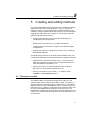
1
UNICORN
version 3.10
for oligonucleotide synthesis
User Manual
18-1134-71
Edition AA
BioPilot, BioProcess, FPLC, FPLCdirector, SMART, UNICORN and
ÄKTA are trademarks of Amersham Biosciences Limited or
its subsidiaries
Amersham and Amersham Biosciences are trademarks of Amersham plc
Compaq is a trademark of Compaq Computer Corporation
Microsoft and Windows are trademarks of Microsoft Corp
Novell and NetWare are registered trademarks of Novell Inc
All goods and services are sold subject to the terms and conditions
of sale of the company within the Amersham Biosciences
group which supplies them. A copy of these terms and conditions is
available on request
© Amersham Biosciences AB 1999 – All rights reserved
Amersham Biosciences UK Limited Amersham Place Little
Chalfont Buckinghamshire England HP7 9NA
Amersham Biosciences AB SE-751 84 Uppsala Sweden
Amersham Biosciences Inc 800 Centennial Avenue
P.O. Box 1327 Piscataway NJ 08855 USA
Amersham Biosciences Europe GmbH Munzinger Strasse 9
D-79111 Freiburg Germany
Preface
Preface
About this manual
This manual provides a full reference to UNICORN TM version 3.10
from Amersham Biosciences AB.
UNICORN is a complete package for control and supervision of
oligosynthesis systems, suitable for use with Amersham
Biosciences' OligoPilot IITM and OligoProcessTM systems. UNICORN
consists of software which runs on an IBM-compatible PC under
Microsoft Windows NT 4.00*, and hardware for interfacing the
controlling PC to the synthesis module.
The manual is organised in 14 chapters and 6 appendices:
Introductory
material
1. Introduction
2. UNICORN concepts
3. Logon and file handling
Methods and
runs
4. Creating methods from method templates
5. Creating and editing methods
6. Performing a run
7. MethodQueues
Evaluation
8. Presenting results
9. Evaluating results
System
management
10. Security features
11. Network setup
12. Installation
13. Administration
14. System settings
Appendices
A. Technical specifications
B. General strategy for oligosynthesis
C. Evaluation functions and instructions
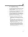
D. Feedback tuning
E. File organisation
F. Troubleshooting
*Microsoft Windows NT and other Microsoft products mentioned in this User Manual are
trademarks or registered trademarks of the Microsoft Corporation.
i
Preface
Assumptions
Two broad assumptions are made in this manual:
1. You should be familiar with the oligosynthesis systems in your
installation. Refer to the appropriate System Manuals for details.
2. You should be familiar with the general principles of using
Microsoft Windows NT version 4.0 on your PC. Although
UNICORN is a self-contained program package and does not
require any direct interaction by the user with Windows NT, the
user interface principles follow the conventions set by Windows
NT programs.
Many of the menu commands in UNICORN can be activated
using the toolbar buttons, keyboard shortcuts and the right mouse
button menu. The availability of these command options is
dependent on the active field or window in which you are currently
working. The function of a toolbar button is displayed when you
place the mouse pointer over a button. Right mouse button menu
commands are quickly found through use of the program.
Typographical conventions
Menu commands, the names of dialogue boxes and windows, the
contents of dialogue boxes windows, and option buttons are written
with a bold helvetica typeface. Menu commands are written in the
order of the menu name and then the command, separated by a colon.
For example:
“Select File:Save As to display the Save As dialogue. Locate the
destination drive and folder and enter a file name. Click on Save.”
This directs you to click on the File menu and select the command,
Save As. A dialogue called Save As is displayed in which you must
locate the destination folder for the saved file and give the file a name.
You then click on the button called Save in the dialogue to execute the
save command.
A typewriter-like typeface is used for instructions as they appear
in the text editor for methods and evaluation procedures. These are
normally entered automatically by UNICORN.
Some menu commands also have shortcut keys on the keyboard, which
are written within < > marks.
ii
Contents
Contents
Introductory material
1 Introduction
2 UNICORN concepts
2.1 UNICORN control software
2-1
2.1.1 Strategies
2-1
2.2 UNICORN user interface
2-2
2.2.1 Toolbar Guide
2.2.2 Software modules
2.2.3 On-line help
2-2
2-2
2-3
2.3 Files and folders
2-3
2.3.1 Method files
2.3.2 Result files
2-3
2-4
2.4 Methods
2-4
2.4.1 Method structure
2.4.2 Method templates
2-4
2-7
2.5 System control
2-7
2.5.1 Control facilities
2.5.2 System connections
2-7
2-8
2.6 Evaluation
2-9
2.7 Network considerations
2-10
2.7.1 Stand-alone installation
2.7.2 Network control from a remote workstation
2-10
2-10
2.8 Security
2-11
3 Logon and file handling
3.1 Logging on
3-1
3.2 Toolbar Guide
3-2
3.3 UNICORN Main menu windows
3-5
Contents
3.3.1 Creating a new folder
3.3.2 Opening and running method files
3.3.3 Presenting files
3.3.4 Finding files
3.3.5 Copying and moving files and folders
3.3.6 Deleting files
3.3.7 Renaming files
3.3.8 Backup security
3-5
3-5
3-6
3-8
3-9
3-13
3-13
3-14
3.4 Printer setup
3-14
3.4.1 Setting the margins
3-14
3.5 Logging off
3-15
3.6 Quitting UNICORN
3-15
Methods and runs
4 Creating methods from method templates
4.1 Creating a new method
4-1
4.2 Saving and running a test sequence method
4-3
4.3 Creating a sequence and method
4-4
4.4 Editing method variables
4-7
4.5 Method notes
4-9
4.6 Saving the method
4-10
4.7 Starting a run
4-11
4.8 Editing text instructions
4-12
5 Creating and editing methods
5.1 The sequence editor
5-1
5.1.1 Modifying cross references in the sequence editor
5-2
5.2 Text instruction editor
5-6
5.2.1 Run setup
5-8
5.3 Method blocks
5-8
5.3.1 Viewing blocks
5.3.2 Calling blocks
5.3.3 Adding blocks
5-8
5-10
5-11
Contents
5.3.4 Deleting blocks
5.3.5 Renaming blocks
5.3.6 Copying, moving and importing blocks
5-13
5-14
5-14
5.4 Method instructions
5-17
5.4.1 Viewing instructions
5.4.2 Adding instructions
5.4.3 Deleting instructions
5.4.4 Changing instructions
5.4.5 The flow scheme window
5-17
5-19
5-20
5-21
5-23
5.5 Method variables
5-23
5.5.1 Identifying variables
5.5.2 Defining variables
5.5.3 Removing a variable
5.5.4 Renaming a variable
5-24
5-24
5-26
5-26
5.6 Run setup
5-26
5.6.1 Variables
5.6.2 Questions
5.6.3 Notes
5.6.4 Evaluation procedures
5.6.5 Method Information
5.6.6 Sequence
5.6.7 Result Name
5.6.8 Start protocol
5-26
5-27
5-31
5-32
5-36
5-36
5-36
5-38
5.7 Saving the method
5-40
5.7.1 Saving a method
5.7.2 Saving as a template
5.7.3 Deleting a template
5-40
5-41
5-42
5.8 Printing the method
5-42
5.9 How to use selected unconditional method instructions 5-43
5.9.1 Base instruction
5.9.2 Instructions at the same breakpoint
5.9.3 Block and method length
5.9.4 Messages and set mark
5.9.5 Pausing a method
5.9.6 Linear flow rates
5-43
5-44
5-45
5-47
5-48
5-49
5.10 How to use selected conditional method instructions
5-49
5.10.1 Standard Watch conditions
5-49
Contents
6 Performing a run
6.1 Starting a method
6-1
6.1.1 Starting from the Main menu
6.1.2 Starting from System control
6.1.3 Starting an Instant Run
6.1.4 Start protocol
6-2
6-2
6-3
6-3
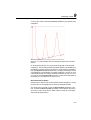
6.2 Monitoring a run
6-5
6.2.1 General window techniques
6.2.2 Run data
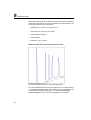
6.2.3 Curves
6.2.4 Flow scheme
6.2.5 Logbook
6.2.6 Synthesis Data
6-5
6-5
6-8
6-14
6-14
6-15
6.3 Manual control
6-16
6.3.1 The toolbar
6.3.2 Manual instructions
6.3.3 Alarms and warnings
6-16
6-18
6-19
6.4 If communication fails
6-20
6.5 Managing system connections
6-20
6.5.1 Establishing a connection
6.5.2 Connection modes
6.5.3 Leaving and locking a system
6.5.4 Disconnecting a system
6.5.5 Network considerations
6-20
6-21
6-22
6-23
6-24
6.6 Calibrating monitors
6-24
6.7 Maintenance
6-26
6.7.1 Viewing system component information
6.7.2 Setting up maintenance warnings
6.7.3 Viewing and zeroing the warning parameters
6.7.4 Getting a warning
6-27
6-28
6-30
6-30
7 MethodQueues
7.1 Setting up a MethodQueue
7-1
7.1.1 Defining a MethodQueue
7.1.2 MethodQueue folders and icons
7-1
7-4
7.2 Editing MethodQueues
7-4
Contents
7.3 Running a MethodQueue
7-5
7.3.1 Method execution in MethodQueues
7-5
7.4 Displaying MethodQueues
7-6
Evaluation
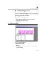
8 Presenting results
8.1 Opening a result file
8-1
8.1.1 Chromatogram
8.1.2 Temporary chromatogram
8-2
8-2
8.2 Basic presentation of chromatograms
8-2
8.2.1 The chromatogram window
8.2.2 Opening the Chromatogram Layout dialogue
8.2.3 Choosing the curve(s) you want to see
8.2.4 Changing curve names
8.2.5 Changing the colour and style of curves
8.2.6 Defining and positioning curve text
8.2.7 Changing and fixing the axes
8.2.8 Viewing information about the run
8.2.9 Saving and applying a layout
8.2.10 Viewing a grid in the chromatogram window
8-3
8-4
8-5
8-5
8-6
8-7
8-7
8-9
8-9
8-10
8.3 Other presentation possibilities
8-10
8.3.1 Showing part of a curve
8.3.2 Reducing noise and removing ghost peaks
8.3.3 Subtracting a blank run curve
8.3.4 Adding curves
8.3.5 Entering text in the chromatogram
8.3.6 Renaming chromatograms, curves and peak tables
8-10
8-13
8-14
8-17
8-17
8-18
8.4 Comparing different runs
8-18
8.4.1 Comparing chromatograms from different runs
8.4.2 Comparing curves
8.4.3 Stacking and stretching curves
8.4.4 Mirror images of curves
8-18
8-22
8-27
8-31
8.5 Saving results
8-32
8.6 Printing active chromatograms
8-32
8.7 Printing reports
8-33
Contents
8.7.1 Creating a new customised report format
8.7.2 Creating a new standard report format
8.7.3 Modifying an existing report format
8-34
8-47
8-50
8.8 Run documentation
8-51
8.9 Exiting Evaluation
8-55
9 Evaluating results
9.1 Integrating peaks
9-1
9.1.1 Baseline calculation for integration
9.1.2 Performing a basic integration
9.1.3 Optimising peak integration
9.1.4 Optimising the baseline parameters using a
morphological algorithm
9.1.5 Optimising the baseline parameters using a c
lassic algorithm
9.1.6 Manually editing a baseline
9.1.7 Adjusting the peak limits
9.1.8 Measuring retention time and peak heights
9.1.9 Measuring HETP
9.1.10 Measuring peak asymmetry
9.1.11 Measuring resolution
9-1
9-2
9-4
9-11
9-18
9-20
9-23
9-24
9-25
9-25
9.2 Other evaluations
9-26
9.2.1 Peak purity and peak identification
9.2.2 Finding the slope values for Peak Fractionation or
Watch instructions
9.2.3 Creating a curve
9.2.4 Measuring salt concentrations in the fractions
9-26
9.3 Automated evaluation procedures
9-33
9.3.1 Recording a procedure
9.3.2 Editing an existing procedure
9.3.3 Renaming and removing procedures
9.3.4 Points to watch
9.3.5 Running evaluation procedures
9.3.6 Batch runs
9.3.7 Evaluation procedures and reports
9.3.8 Placing a procedure on the menu and running
9.3.9 Exporting data or curves
9.3.10 Exporting results
9.3.11 Copying results to the clipboard
9.3.12 Importing results and curves
9-33
9-35
9-37
9-37
9-38
9-38
9-40
9-41
9-41
9-41
9-43
9-43
9-8
9-28
9-30
9-32
Contents
System management
10 Security features
10.1 Access security
10-1
10.2 Connection security
10-1
10.3 Data security
10-2
10.3.1 Network communication failure
10.3.2 Local station failure
10-2
10-3
10.4 Security recommendations for control stations
10-3
11 Network setup
11.1 Introduction
11-1
11.2 Requirements
11-4
11.3 Installation guide
11-5
11.3.1 TCP/IP - NT domain
11.3.2 IPX/SPX - Novell server
11-5
11-10
12 Installation
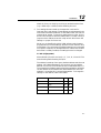
12.1 Installation summary
12-1
12.2 Migrating from UNICORN OS 1.10 to UNICORN 3.10
12-1
12.2.1 Before migration
12.2.2 Migration and post-installation setup
12-1
12-2
12.3 System requirements
12-2
12.4 Hardware installation
12-2
12.5 Software installation
12-6
12.5.1 Installing UNICORN for the first time
12.5.2 Installing selected software components after the
initial installation
12-6
12-18
13 Administration
13.1 System definitions
13-2
13.1.1 Defining new systems
13.1.2 Editing system definitions
13-2
13-4
Contents
13.1.3 Deleting system definitions
13-4
13.2 Access levels
13-4
13.2.1 Defining access levels
13.2.2 Access level examples
13-4
13-7
13.3 User administration
13-9
13.3.1 Defining new users
13.3.2 Changing user passwords
13.3.3 Viewing and changing user definitions
13.3.4 Deleting users
13.3.5 Defining new home folders
13.3.6 Deleting home folders
13.3.7 Printing user setup information
13-10
13-12
13-12
13-12
13-13
13-13
13-14
13.4 Audit trails
13-14
13.4.1 Examining audit trails
13.4.2 Renewing audit trail files
13.4.3 Backing up audit trail files
13-14
13-17
13-17
13.5 Report Generator Wizard
13-18
13.5.1 Generating a report from the main menu
13.5.2 Generating a report from System Control
13-19
13-22
14 System settings
14.1 Alarms
14-2
14.2 Specials
14-4
14.3 Curves
14-5
Appendices
A Technical specifications
A.1 System requirements
A-1
A.1.1 Hardware requirements
A.1.2 Software requirements
A.1.3 Network requirements
A-1
A-1
A-2
A.2 Control capacity
A-2
A.2.1 Stand-alone installations
A.2.2 Network installations
A-2
A-2
Contents
A.3 Data sampling
A-3
B General strategy for Oligo Synthesis
B.1 Method instructions
B-1
B.1.1 Pump
B.1.2 Flowpath
B.1.3 Alarms&Monitors
B.1.4 Watch
B.1.5 Other
B-1
B-4
B-6
B-7
B-8
B.2 Manual control
B-9
B.2.1 Pump
B.2.2 Flowpath
B.2.3 Alarms&Monitors
B.2.4 Other
B-9
B-9
B-9
B-10
B.3 System settings instructions
B-10
B.3.1 Alarms
B.3.2 Specials
B.3.3 Monitors
B.3.4 Curve
B.3.5 Method variables
B-10
B-11
B-12
B-13
B-13
C Evaluation functions and instructions
C.1 Smoothing algorithms
C-1
C.1.1 Moving Average
C.1.2 Autoregressive
C.1.3 Median
C-1
C-1
C-2
C.2 Baseline calculation theory
C-2
C.2.1 Defining baseline segments
C.2.2 Selecting baseline points (for Classic algorithm)
C.2.3 Drawing the baseline
C.2.4 Estimating the baseline parameters from the source
curve (for Classic algorithm)
C.2.5 Measuring the Slope limit using Differentiate and
curve co-ordinates (for Classic algorithm)
C-3
C-5
C-5
C.3 Peak table column components
C-7
C-5
C-6
C.4 Evaluation procedure
C-12
C.4.1 Curve operations
C-12
Contents
C.4.2 Integration
C.4.3 File Operations
C.4.4 Export
C.4.5 Chromatogram functions
C.4.6 Other
C-15
C-16
C-17
C-21
C-22
D Feedback tuning
D.1 Flow rate tuning
D-2
D.2 Gradient tuning
D-3
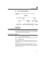
E File organisation
E.1 Stand-alone installations
E-1
E.2 Network installations
E-1
E.2.1 Local and remote computers
E.2.2 Network server
E-1
E-1
F Troubleshooting
F.1 Logon problems
F-1
F.1.1 Unable to log on to UNICORN
F.1.2 Error message "Strategy file error"
F-1
F-1
F.2 UNICORN access problems
F-1
F.2.1 Unable to access certain UNICORN functions
F.2.2 Connections are not available
F.2.3 Run data Connection in System control displays a “No x”
F-1
F-2
F-2
F.3 Method and run problems
F-3
F.3.1 Cannot Quit or Logoff from UNICORN
F-3
F.3.2 Monitor signals do not appear in the system control
Curves panel
F-3
F.3.3 Error message "Couldn't create result file"
F-3
F.3.4 The Method-System Connection dialogue keeps appearing F-3
F.3.5 The method editor window does not fit on the screen
F-4
F.3.6 There are red instructions in a method
F-4
F.3.7 I’ve logged out of Windows NT and then logged in
again but I can not get system connection in
UNICORN (only for local systems, not remote)
F-5
F.3.8 Print screen does not send a copy of the screen to the printer F-5
F.4 Evaluation problems
F-5
Contents
F.4.1 Incorrect date and time
F.4.2 Evaluation procedure aborts
Index
F-5
F-5
Contents
Introductory material
Methods and runs
Evaluation
System management
Appendices
Introduction
1
1
Introduction
UNICORN is a control system developed and marketed by Amersham
Biosciences AB for real-time control of oligosynthesis systems
from a personal computer. The package operates together with
OligoPilot II and OligoProcess from Amersham Biosciences.
UNICORN runs under the operating system Microsoft Windows NT
version 4.0.
Functional features of UNICORN 3.10 include:
• One PC may control up to 4 oligosynthesis systems directly.
• Network support allows up to 90 systems to be run from one PC.
• Method templates, providing method frameworks for most
common applications, eliminating the need to program methods
from scratch.
• Modular method definition in the method templates, reflecting the
separate steps in a process.
• Dynamic graphical overview of active runs.
• User-definable alarm and warning limits for monitor signals.
• Programmed sequential operation.
• Batch operation and process documentation in accordance with
the requirements of Good Manufacturing Practice (GMP) and
Good Laboratory Practice (GLP).
• Comprehensive data evaluation software.
In addition, UNICORN offers a comprehensive security system:
• Password control for all users, with access authorisation for other
users' method and result files.
• Customised definition of access control levels.
• Audit trail for system operation.
Note: UNICORN must be correctly installed for stand-alone or
network operation before the software can be used. Network
considerations, software installation and administration of
system and user definitions are described in Chapters 11, 12
and 13.
1-1
1
1-2
Introduction
UNICORN concepts
2
2
UNICORN concepts
This chapter introduces the basic concepts that are specific to
UNICORN. For a description of how to work with the Windows NT
operating system, see your Windows NT system documentation.
Material in this chapter is divided into 8 sections, dealing with:
• UNICORN control software
• UNICORN user interface
• Files and folders
• Methods and method structure
• System control
• Evaluation
• Network considerations
• Security and administration
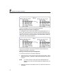
2.1 UNICORN control software
UNICORN runs under the Windows NT operating system, and
provides facilities for method-controlled operation of oligosynthesis
systems as well as real-time monitoring and subsequent evaluation of
the synthesis process.
2.1.1
Strategies
Part of UNICORN software (referred to as the strategy) is system
specific. The strategy defines what is available in method and manual
instructions, system settings, run data, curves and method templates.
Most of this manual describes the user interface in UNICORN
independent of the strategy. Strategy-dependent instructions are listed
in Appendix B.
2-1
2
UNICORN concepts
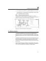
2.2 UNICORN user interface
2.2.1
Toolbar Guide
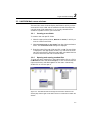
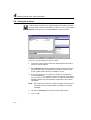
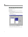
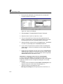
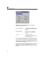
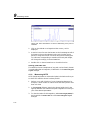
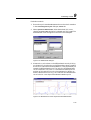
The UNICORN Toolbar Guide dialogue is shown after start-up and
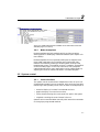
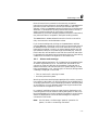
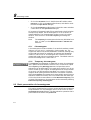
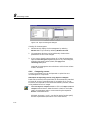
logon reminding you about the Main menu toolbar buttons.
Figure 2-1. UNICORN Toolbar Guide dialogue.
The Main menu toolbar buttons allow you to begin using UNICORN
quickly, for example, to create a new method in the Method editor,
start an instant run, open a result file for evaluation, or execute manual
instructions in System control (see Section 3.2).
2.2.2
Software modules
UNICORN control software consists of four integrated modules:
• The Main menu, with functions for file handling and
administrative routines such as definition of available
oligosynthesis systems and maintenance of user profiles.
• The Method editor, where methods for pre-programmed control of
oligosynthesis systems are created and edited.
2-2
UNICORN concepts
2
• The System control module, which permits manual or methodbased control of oligosynthesis systems and on-line monitoring of
synthesis processes. There may be up to four independent system
control modules on one computer, for controlling up to four
separate systems.
• The Evaluation module, with extensive facilities for presenting and
evaluating stored results from synthesis processes.
These modules are present on the Windows NT taskbar.
To minimize a module to the taskbar, click on the Minimize button at
the right-hand end of the window title bar. To minimize the whole of
UNICORN click on the <Windows + M> keys on the keyboard.
Note:
Minimizing a module window to the taskbar does not close
the module. Once opened, UNICORN modules remain
active until you quit the program. A minimised System
control module may thus be actively in control of a running
process.
2.2.3
On-line help
A comprehensive on-line help utility is included in UNICORN
software. Entry to the general help utility can be accessed from the
Help menu. Dialogue- or window-specific help topics can be obtained
by clicking on the Help button in the dialogue or by pressing <F1> on
the keyboard. In the dialogues for method instructions, procedure
instructions and system settings, pressing <F1> when an instruction is
highlighted will display an information box with short help on the
function and use of the selected instruction.
2.3 Files and folders
UNICORN Main menu interface divides user files into two categories,
for methods and results (see Figure 2-1). Only folders to which the
current user has access are shown in the Main menu windows, Method
window and Results window. Files may be displayed in several
viewing options (see Chapter 3 for more details).
2.3.1
Method files
Method files contain instructions for controlling a run and are shown
in the Methods window of the Main menu.
The Methods window also displays icons for MethodQueues, which
allow several methods to be run in an automatic pre-programmed
sequence on the same or different systems.
2-3
2
UNICORN concepts
2.3.2
Result files
Result files are created by UNICORN when a method is run and
contain:
• A copy of the method used in the run.
• Run data from the monitors in the oligosynthesis system (e.g. UV
absorbance, flow rate, conductivity etc.).
• Saved results from evaluation of the run data (see Chapter 10).
• Run documentation including information on, for example, the
run log, calibration settings, scouting parameters, text method etc.
2.4 Methods
Oligosynthesis runs are programmed as methods in UNICORN. This
section gives a brief overview of the concepts and principles of
methods. See Chapters 4 and 5 for a description of how to program
methods, and Chapter 6 for how methods are used to control
oligosynthesis systems.
2.4.1
Method structure
Blocks
Methods in UNICORN are divided into blocks. Blocks typically
contain the subroutines that control the complete synthesis procedure.
A synthesis cycle is generally based on the following order of
subroutines:
• Detritylation
• Detrit wash
• Coupling
• Oxidation/thiolation
• Capping
Method templates supplied with UNICORN contain all the blocks
that are likely to be used in a specific method. When the desired
sequence is created, the blocks needed to build up the method to
synthesize the sequence are automatically copied in from the method
template. The methods derived from the method templates can be
directly used to process the run.
Additionally, the methods are convenient starting points for
developing customized methods. Fully adequate customised methods
for many applications can be created simply by adjusting the values of
2-4
UNICORN concepts
2
method variables (see below). New blocks can also be created in the
Text instructions or in the cross reference list of the Sequence page in
Run setup.
Method base
Method blocks are written in one of three method bases, which defines
the unit for the breakpoints in the block:
• time (min)
• volume (ml or l according to the strategy)
• column volume (set by the user)
Different blocks in the same method may be written with different
method bases: for example a column wash block might be written in
terms of column volumes while a purge block might be best expressed
in absolute volume.
Note:
The term method base should not be confused with bases in a
sequence or an oligonucleotide.
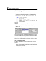
Instructions
The method is a call to blocks, with each block containing a series of
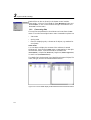
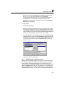
instructions or sub-routines (see Figure 2-2). Each instruction is a
request for specific operations in the system. A block may also contain
other blocks which in turn contain their own series of instructions.
Double click on a block to expand/collapse the view of the
instructions.
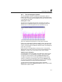
Figure 2-2. Relationship between blocks and instructions. The method (left)
is written as a series of calls to blocks, each of which consists of instructions
for performing one or more specified tasks (right).
2-5
2
UNICORN concepts
Breakpoints
Each instruction in a method block is issued at a specified breakpoint
according to the method base. The first instruction in a block is always
at breakpoint 0, and all other breakpoints are counted from this point.
For example, in the following instructions from a block:
0.00
Base Time
0.00
Flow_Reag 5.00 {ml/min}
9.00
Flow_Reag 0.00 {ml/min}
At breakpoint 0.00, the reagent flow rate is set to 5.00 ml/min. After
nine minutes have elapsed, at the next breakpoint, the flow rate of the
reagent will be set at 0.00 ml/min, i.e. no flow at all.
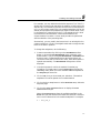
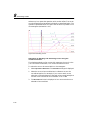
Method variables
Breakpoint values and instruction parameters may be defined as
variables. This is a powerful facility for constructing a method which
contains default parameter values. These default values may then
easily be changed either to create variants of the same method or to
adjust the parameter values at the start of a run (see Section 4.4).
Using variables makes it easy to adapt a method to a particular
oligonucleotide synthesis run. For example, in the block below, the
values of the start parameters variables can be seen:
(START parameters)
0.00
Base SameAsMain
0.00
Scale (2)#Weight_of_support {g},
(90)#Loading_of_support {umol/g}
0.00
DelayVol 2.00 {ml}
0.00
ColDiam (20)#Col_Diam {mm}
4.00
End_block
The variables are expressed:
(variable value)#Variable_type {variable units}
In the block above, it is possible to see that the variable values have
been set at 2 g weight of support, 90 µmol/g loading of support and a
20 mm column diameter.
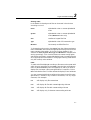
By using variables, a method may be displayed either in detail as text
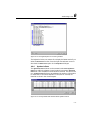
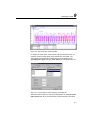
instructions or in a condensed form as variable values in Run setup
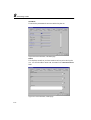
mode. This is illustrated in Figure 2-3. The Run setup mode is
displayed when the method is run, allowing variable values to be set at
the beginning of the run.
2-6
UNICORN concepts
2
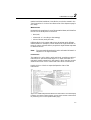
Figure 2-3. Relationship between variables in text instructions and in the
Variables page of run set-up.
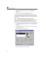
2.4.2
Method templates
Method templates are basic methods which provide convenient
starting points for developing customised methods (see Chapter 4 for
more details).
Method templates for most synthesis techniques are supplied with
UNICORN installations for OligoPilot and OligoProcess. New
methods are created by selecting a suitable system, technique and
template and column. The method can then, if necessary, be modified
on the Variables page or in the Text instructions. Fully adequate
customised methods for many applications can be created simply by
adjusting the values of method variables in a suitable template.
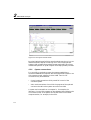
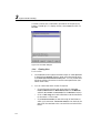
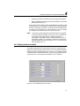
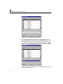
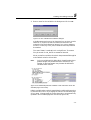
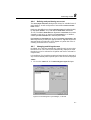
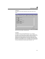
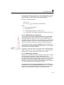
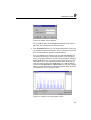
2.5 System control
2.5.1
Control facilities
The system control module allows independent control of up to four
oligosynthesis systems from one computer, with continuous real-time
monitoring of the synthesis process. The run status can be displayed as:
• numerical display of run data from selected monitors
• graphical display of curves from monitors
• a flow scheme showing the current open flow path in the system
• a logbook recording the control events in the run.
Systems can be controlled either manually with interactive commands
or through pre-programmed methods.
2-7
2
UNICORN concepts
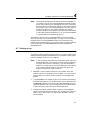
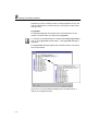
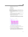
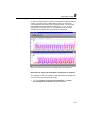
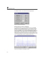
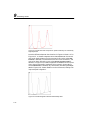
Figure 2-4. The system control screen.
By using MethodQueue facilities, several methods may be run in a predefined automatic sequence involving one or more oligosynthesis
systems. With suitable oligosynthesis system equipment, this allows
unattended operation of quite complex multi-step synthesis processes.
2.5.2
System connections
For controlling a synthesis process, the operator establishes a
connection between the computer and the oligosynthesis system in one
of the system control windows in UNICORN. Two kind of
connections may be established:
• Control mode connections which permit full control of the
connected system.
• View mode connections from which the progress of the synthesis
can be monitored but the system cannot be controlled.
A system can be started from a computer in, for example, the
laboratory. Control of the system can be released without affecting the
run and the control of the system can be later taken from another
computer station, for example, in the office.
2-8
UNICORN concepts
2
Each oligosynthesis system can have only one control mode connection
at any one time, but it can have several view mode connections. In a
network installation, the same or different users may establish
simultaneous view mode connections to one system on different
computers. This allows a running process to be monitored from several
locations at the same time.
2.6 Evaluation
The evaluation module (chapter 9 and 10) provides extensive facilities
for presentation and evaluation of synthesis results. Essential features
of evaluation include:
• Trityl data. This is stored in the result file and can be printed in a
report as a table
• Curve manipulation. A wide range of operations can be performed
on curves, such as addition and subtraction of two curves,
differentiation, integration, normalization and scaling. The
original raw data curves are always kept unmodified in the result
file.
• Curve comparisons. Curves from different result files can easily be
compared in the evaluation module.
• Evaluation procedures. Operations performed in the evaluation
module can be recorded as an evaluation procedure and repeated
for other result files with a single menu command. Evaluation
procedures may be executed either automatically on completion of
a method run or interactively from within the evaluation module.
• Reports. Comprehensive reports of the evaluation results can be
generated for hard-copy documentation of the synthesis process.
Generation and printing of reports may be included as an
operation in an evaluation procedure to automate process
evaluation and documentation.
2-9
2
UNICORN concepts
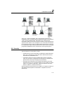
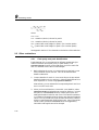
2.7 Network considerations
UNICORN can be installed on a stand-alone PC workstation and/or
PC workstations in a network.
2.7.1
Stand-alone installation
In a stand-alone installation, up to four oligosynthesis systems may be
physically connected to and controlled from the workstation where
UNICORN is installed.
Figure 2-5. Stand-alone installation of UNICORN on a workstation, which can
control up to four separate oligosynthesis systems.
2.7.2
Network control from a remote workstation
In a network installation, each oligosynthesis system is physically
connected to a workstation, but may be controlled from any
workstation in the network on which the UNICORN software is
installed. A workstation to which a system is physically connected is
referred to as a local station. Other workstations in a network
installation are called remote stations.
During installation of UNICORN for the first time on a workstation
in a network configuration, certain files are copied to the network
server. These files include UNICORN user files and strategy files, and
are the global settings for all UNICORN users in the network (see
Chapter 13). However, UNICORN program files and templates are
NOT copied or located on the network server and as such the server
cannot be used to control a run. UNICORN program files and
templates are instead locally installed on each workstation in the
network, and the network is used as the medium of communication to
establish control with the oligosynthesis systems.
2-10
UNICORN concepts
2
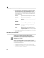
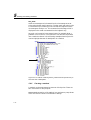
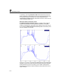
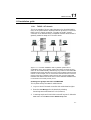
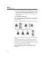
Figure 2-6. A network installation with 4 oligosynthesis systems and 5
workstations (PCs). The oligosynthesis systems physically connected to PCs
1 and 5 can be controlled locally. Alternatively, any of the PCs with
UNICORN installed can be used to remotely control any of the oligosynthesis
systems via the network. In this example, PC 4 is connected to the network
but it cannot be used to control any oligosynthesis systems since it does not
have UNICORN installed. Note also that the server does not have UNICORN
program files installed and is not involved in the control process per se.
2.8 Security
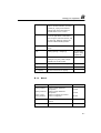
Security features in UNICORN include:
• Access security. Use of UNICORN is restricted to authorised users.
Each user is assigned an access level which defines the functions
that the user is permitted to use.
• Connection security. Running systems may only be controlled
from one connection. Systems may be locked with a password to
prevent other users from changing run parameters.
• Data security. Result files can be saved automatically at pre-set
intervals during a run to minimise data loss in the event of system
failure. In a network installation, results are saved on the local
station if network communication fails.
Security features are discussed in more detail in Chapter 10. Network
and administrative aspects are discussed in Chapters 13 and 14
respectively.
2-11
2
2-12
UNICORN concepts
Logon and file handling
3
3
Logon and file handling
3.1 Logging on
When you start the computer you must log on to Windows NT before
you can log on to UNICORN and begin working. Logging on to
Windows NT will automatically connect you up to the network if NT
has been so configured. Network connection is not essential for local
control of a system.
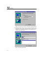
1. To start UNICORN, locate the program in the Windows NT Start
button under Programs:Unicorn:Unicorn 3.10. Alternatively,
double click on the UNICORN icon on the desktop if this option
was selected during installation.
If UNICORN is already started and the previous user has logged
off, click on the Logon menu command or click on Logon/Logoff
button the in the Main menu module.
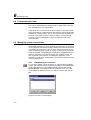
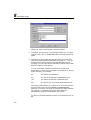
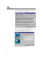
Figure 3-1. The Logon dialogue.
Click on your username in the list and type your password. Click
on the OK button to log on. If you cannot remember your
password, you cannot log on to UNICORN. Ask your system
administrator or other user with sufficient authorisation to give
you a new password.
Note:
If UNICORN has been installed so that no password is
required for logon, you need only select you username and
click on OK to proceed.
3-1
3
Logon and file handling
Press the Cancel button to abandon the logon attempt.
Network installations
In a network installation, you must be logged on to the network before
starting UNICORN. Any computer station in the network with
UNICORN software installed can be used to log on to UNICORN.
You can log on with the same username and password on multiple
computers simultaneously.
Each oligosynthesis system can have only one control mode connection
at any one time, but it can have several view mode connections. In a
network installation, the same or different users may establish
simultaneous view mode connections to one system on different
computers. This allows a running process to be monitored from several
locations at the same time. Multiple logons with the same username
are treated internally as separate users for the purpose of System
control.
Note:
Do not confuse Windows NT/network logon with
UNICORN logon. You log on to the network to gain access
to network resources (shared drives, printers and other
networked equipment). You log on to UNICORN to gain
access to the oligosynthesis systems that are installed in the
network. The username and password for logging on to the
network are entirely independent of the those for logging on
to UNICORN.
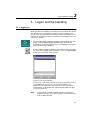
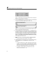
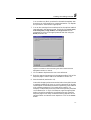
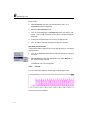
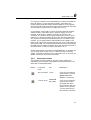
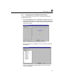
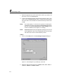
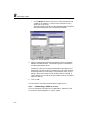
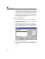
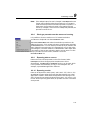
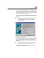
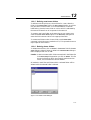
3.2 Toolbar Guide
The UNICORN Toolbar Guide dialogue is shown after start-up and
logon reminding you about the Main menu toolbar buttons.
The Main menu toolbar buttons allow you to begin using UNICORN
quickly, for example, to create a new method in the Method editor,
start an instant run, open a result file for evaluation, or execute manual
instructions in System control.
3-2
Logon and file handling
3
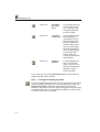
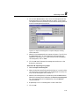
Figure 3-2. UNICORN Toolbar Guide dialogue.
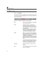
The toolbar buttons are:
About UNICORN
This gives you information about the
UNICORN version installed, copyright
and web address for obtaining more
information.
Logon/Logoff
This allows you to log on or off
UNICORN as appropriate.
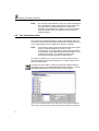
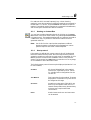
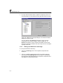
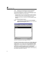
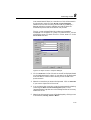
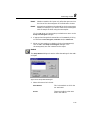
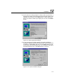
Instant Run
This opens the Instant run dialogue (Fig. 33) in which you can select the system to
run, technique and template. Press on the
Run button to view the Start protocol and
to start the run (see Chapter 6).
3-3
3
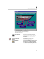
Logon and file handling
Figure 3-3. Instant Run dialogue.
Note:
3-4
Use of this function requires that templates are defined.
Standard systems are supplied with templates, but custom
systems require that the user makes templates.
New Method
This immediately starts the Method editor
module and displays the New Method
dialogue (see Section 4.1).
System Control
This activates the first connected System
control and displays the Manual instruction
dialogue (see Section 6.3.2).
Evaluation
This displays the Open result dialogue.
Select a result file and click on OK to launch
the Evaluation module (see Chapter 9).
Logon and file handling
3
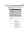
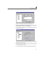
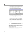
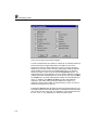
3.3 UNICORN Main menu windows
The two Main menu windows display the folders to which you have
access within UNICORN and the method and result files within the
currently open folder respectively. You can only see method files
written for systems to which you have access.
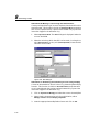
3.3.1
Creating a new folder
To create a new user-specific folder:
1. Select the appropriate window, Methods or Results, in which you
want to create a new folder.
2. Select File:New:Folder or New Folder from the right mouse button
menu. The Create New Folder dialogue is displayed.
3. Enter the name of the new folder and click on OK. The new folder
is displayed in the appropriate window. Any user that has access
set to the main folder in which the new folder was created also has
access to the folders and files contained therein.
3.3.2
Opening and running method files
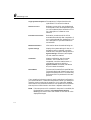
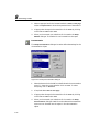
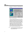
To open and edit a method file in the Method editor click on a file in
the Methods window and select File:Open, or click on the file with the
right mouse button and select Open from the menu. Alternatively,
double click on a file to open it.
Figure 3-4. The Method window with right mouse button selected in the
window (left) and the right mouse button menu for a selected icon within the
window.
3-5
3
Logon and file handling
Method files can be run directly in the System control module.
Alternatively, click on a file in the Main menu Methods window and
select File:Run, or click on the file with the right mouse button and
select Run from the menu.
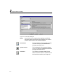
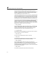
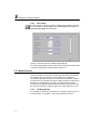
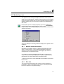
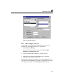
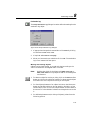
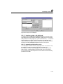
3.3.3
Presenting files
The way files are presented in the windows can be set from the File
menu or from the mouse right button menu. Presentation options are:
• view mode
• sorting order
• filter (for displaying only a chosen set of objects, e.g. methods for
one system)
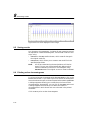
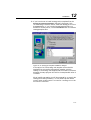
View mode
You can select to display the contents of the windows in several
Windows NT views from the View menu or View options in the right
mouse button menus. View the files either as a details list
(View:Details), a simple list (View:List), large icons (View:Large Icons)
or small icons (View:Small Icons).
The details list includes a small icon identifying the type of object, file
name, file type, and the last modified date and time.
Figure 3-5. Icon and detail display modes illustrated for the Methods window.
3-6
Logon and file handling
3
Sorting order
In the details list viewing mode files can be sorted in the window
according to one of:
Name
alphabetical order or reverse alphabetical
order
System
alphabetical order or reverse alphabetical
order (Method window only)
Size
smallest or largest files first
Type
alphabetical order of file extension type
Modified
last recently modified files first
To change the sorting order, choose Sort from the right mouse button
menu or File:Sort, and choose the appropriate sorting order from the
menu cascade. Alternatively, click on the column headers in the
window for Name, System, Size, Type and Modified to change the file
sorting accordingly. Click a second time on the same sorting option
and the files are sorted in reverse alphabetical order, increasing file size
etc. as appropriate to the selection. Changing the sorting order affects
only the currently active window.
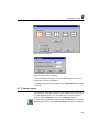
Filter
To restrict the files displayed according to file name or the system with
which they are associated, choose Filter from the right mouse button
menu or select File:Filter. Mark the system(s) for which you want to
display files, and enter a file name specification if required. Click on
OK to activate the filter. The filter affects the display in both windows.
You can use standard Windows wildcard characters in the file name
specification (* stands for any number of characters, ? for any single
character). For example:
test
will display only files named test
test*
will display all files with names beginning with test
*test
will display all files with names ending with test
?test
will display only 5-character names ending with test
3-7
3
Logon and file handling
If a filter is active, this is indicated in the title bar of the panel (e.g.
Results : filtered igf*). To display all files, choose Filter and click on
View All.
Figure 3-6. The Filter dialogue.
3.3.4
Finding files
To find a file:
1. Choose Find from the right mouse button menu or select File:Find.
In the displayed Find file dialogue, enter a file name specification
in the Search for files filtered on name field. You can use standard
Windows wildcard characters in the file name specification (see
above under Filter).
2. You can restrict the search further if required:
3-8
•
Choose file type from the pull-down menu for Type (All,
Folders, Method files or MethodQueue files for the Methods
window; All, Folders or Result files for the Results window).
•
Click on Date range and use the slide bar to set the date limits
for the search. Click on OK.
•
Check Search all folders to search through all the folders to
which you have access. If Search all folders is not checked, the
search will be restricted to the current folder and sub-folders
below.
Logon and file handling
3
Figure 3-7. The Find file dialogue.
3. Click on Find when you have entered all parameters. The result of
the search is shown in the Found files box.
4. Double-click on a file in this list to return to the Main menu with
the selected file highlighted in the appropriate window. If you click
on Close (with or without selecting a file), you will return to the
Main menu with the window display unchanged.
3.3.5
Copying and moving files and folders
You can copy and move files and folders to another folder that is
specific to your user logon name. You can also copy or move files to
and from an external drive and folders available on the network. If you
copy or move a folder, all files within the folder will also be copied or
moved.
Copying or moving files and folders
1. Select one or more files or folders in either the Methods or Results
window of the Main menu. To select multiple files or folders, use
the standard Windows function keys <Ctrl> or >Shift>.
2. Click with the right mouse button on any file/folder icon and
choose the Copy or Move command or select File:Copy or
File:Move. The Copy or Move dialogue is displayed respectively.
3-9
3
Logon and file handling
3. Select an available folder or the diskette drive to which you want
to copy or move the file/folder and click on OK. Copied files and
folders are user-specific.
Note 1: You cannot copy or move files between the Methods and
Results windows of the Main menu.
Note 2: Explicit authorisation is required to copy or move files (see
Section 14.2).
Note 3: To copy a file within the same folder, open the file in the
relevant UNICORN module, e.g. a method file in Method
editor or a result file in the Evaluation module, and use the
File:Save as command in the module to save the file with a
different name from the original.
Note 4: When copying to a diskette (a:) use Copy to external so that
the files are automatically compressed.
Note 5: If you are moving a method to another system, you must
always use the Copy to external/Copy from external
functions. this will give you the possibility of connecting the
method to the appropriate system. The extension for the
method file name is used to identify the system for which the
method has been created. An incorrect extension may result
in syntax errors in the method or the method not being
visible in the Methods window of main menu.
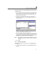
Copying files to external
Copying files to external may be useful when you want to store all
results, documentation etc. in a common project folder on the
network, or want to back up the files in a special place.
To copy a method or result file to external:
1. Select the file to be copied in either the Methods window or Results
window.
2. Select Copy to external from the right mouse button menu or select
File:Copy to external. The Copy to external dialogue is displayed.
3. Select the destination drive and folder and click on the Save
button.
3-10
Logon and file handling
3
Figure 3-8. Copy to external dialogue.
Note:
If you select the 3½” Floppy Drive (a:) as the destination
drive, the files will be automatically compressed into a .zip
file thus allowing approximately 5-10 times the storage
capacity. Moreover, if the zipped file is greater than the
storage capacity of the disk, the file saving is automatically
spanned across several disks. Files are automatically
decompressed when using the Copy from external operation
(see below). The zip function does not work if you select the
Copy function.
Copy files from external
Method and result files can be copied from external. If the selected files
have been compressed using the Copy to external function, then these
will be automatically decompressed. To copy a method or result file
from external:
1. Select the destination folder in the Methods window or Results
window.
2. Without selecting a file icon, bring up the right menu button menu
and select Copy from external or select File:Copy from external.
The Copy from external dialogue is displayed.
4. Select the wanted file(s) from the relevant source drive and folder.
Click on the Save button.
3-11
3
Logon and file handling
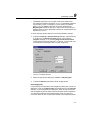
Figure 3-9. Copy from external dialogue, in this example, used to copy
method files.
5. If result file(s) were selected, these will be copied into the
previously designated folder in the Results window.
6. If method file(s) were selected, the Method-System connection
dialogue is displayed.
Figure 3-10. Method-System connection dialogue.
Each copied method listed in the Method files field must in turn be
connected to the same type of system (same strategy) for which the
method was originally created, listed in the Systems field.
Highlight a method and double click on a system. Click on the OK
button.
3-12
Logon and file handling
3
The Method-System connection dialogue is displayed again listing
the remaining methods to be connected. Repeat the process until
all methods have been connected.
Note:
Method syntax errors may arise if a method created on one
system is connected to a different type of system using the
copy from external facility.
If at any time you press on the Cancel button, the Method - System
connection dialogue is closed. However, it will reappear each time
you perform other copy to/from external procedures for method
files.
Method files that have been copied in and connected are displayed
in the previously designated folder in the Methods window.
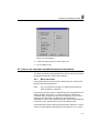
3.3.6
Deleting files
To delete a file or folder:
1. Select the item(s) to be deleted in the Methods or Results window
of the Main menu. To select multiple files, hold down the <Ctrl>
key while you click on the file names or icons.
2. Click with the right mouse button on any file icon and choose
Delete from the menu, or choose File:Delete.
3. Confirm the deletion in the dialogue.
Note 1: Home folders cannot be deleted by this method (see Section
13.3).
Note 2: Explicit authorisation is required to delete files (see Section
13.2).
Note 3: A file that has been deleted cannot be recovered except by
restoring a back-up copy.
3.3.7
Renaming files
To rename a file or folder:
1. Select a file or folder to be renamed in the Methods or Results
window of the Main menu.
2. Click with the right mouse button on any file icon and choose
Rename from the menu, or choose File:Rename. The Rename
dialogue is displayed
3-13
3
Logon and file handling
3. Enter the new name for the file and click on OK.
3.3.8
Backup security
To protect important data against accidental deletion or loss in the
event of hard disk failure, backup copies should be taken at regular
intervals.
This can be best achieved by having the UNICORN folders on the
server (if available) and working directly from these folders.
Alternatively, you can use the File:Copy to external function to save
files onto the network server. It is standard practice for backups to be
made of the server folders. The responsibility for making backup
copies rests entirely with the user. Amersham Biosciences
cannot undertake to replace method programs lost as a result of
computer failure or other incident.
3.4 Printer setup
UNICORN 3.1 uses the default printer and printer settings installed on
your computer. To change the choice of printer, either change the
default settings in Windows NT or set up your choice of destination
printer for the current working session by selecting File:Printer setup
in the Main menu module and selecting the desired printer.
3.4.1
Setting the margins
The default margins for the printers can be changed:
1. Locate the file UNICORN.INI found under C:\UNICORN\BIN,
for example by using Windows NT Explorer.
2. Double click on the file to open it and locate the following lines:
EVAL
PrintMarginLeft
10
EVAL
PrintMarginRight
5
Eval
PrintMarginTop
5
Eval
PrintMarginBottom 5
The values in the lines set the margins based as a percentage of the
full width and height of the paper.
3. Change the values as appropriate and save the file.
Caution: Do not make any other changes in the UNICORN.INI file
since this may severely affect the function of UNICORN.
3-14
Logon and file handling
3
3.5 Logging off
To log off from UNICORN click on the Logoff button or select the
Logoff menu command.
Processes that are running when you log off will continue to run, and
may be left locked with a locking password or unlocked (see Section
6.5 for more details). If the Method editor module was active at the
time of logoff, it will be re-opened when the same user logs on again.
UNICORN will still be open after a user has logged off, and another
user may log on. We recommend that you always log off when you
leave the computer to prevent other users from accidentally changing
or deleting your files or disturbing your runs.
3.6 Quitting UNICORN
To quit UNICORN and close the program, select File:Quit program in
the Main menu. You will be prompted to save any unsaved data in the
Method editor or Evaluation module. If a run is proceeding when you
quit do not shut down Windows NT or turn off the computer while
the run is in progress.
Note:
You can not quit the program if you are performing a
MethodQueue run.
3-15
3
3-16
Logon and file handling
Introductory material
Methods and runs
Evaluation
System management
Appendices
Creating methods from method templates
4
4
Creating methods from
method templates
UNICORN is supplied with a set of method templates that can serve
as the starting point for creating customised methods. These method
templates are defined with variables for critical parameters in the
synthesis, so that customised methods can be created for most
purposes simply by setting appropriate values for the method
variables. Different templates are provided for different system
strategies. This chapter describes how to create and edit methods at
this level. See Chapter 5 about advanced method editing facilities.
Briefly, the steps in creating a method by editing method variables are
as follows:
1. Click on the New Method toolbar button in the Main menu, or
select File:New:Method in the Main menu or File:New in the
Method editor module. Select a system, technique, template and
column.
2. Choose View:Run setup or press the Run setup button.
3. Adjust the values for the method variables.
4. Read the method notes.
5. Save the method.
Note:
The fastest and easiest way to run a method is to click on the
Instant Run toolbar button in the Main menu. This function
runs a method template and the method is not saved in the
Main menu Methods window. The method may, however, be
recovered from the result file.
4.1 Creating a new method
To create a new method, do one of the following:
• click on the New Method toolbar button in the Main menu
• select File:New:Method in the Main menu
• click on the New Method toolbar button in Method editor
• select File:New in the Method editor
4-1
4
Creating methods from method templates
These alternatives are equivalent. When you choose the command
from the Main menu, the Method editor is opened automatically.
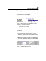
Figure 4-1. The New method dialogue.
1. Choose the system for which the method is intended.
The instructions available for a given system are determined by the
system strategy. A method developed for one system may not be
valid on another.
2. Select Any for the technique. The templates available for the
selected technique will be displayed.
3. A list of ready-to-run method templates is displayed for the
selected technique. Available templates are determined by the
system strategy. Select one of these templates to create customised
methods either by adjusting variable values or changing method
instructions. For your first run you are recommended to select the
method template, Fix Column Recycling Coupling.
Click on a template to display information about the particular
template in the Method notes field.
4. Choose a specific column to be used. Only columns for the selected
technique are displayed. If you do not find your specific column it
can be added to the list (see Section 5.9). Relevant column data are
automatically copied into the method thus reducing the need to
edit the method.
4-2
Creating methods from method templates
4
If Any is selected, you can use any column but must enter the
column volume in the method on the Variables page. It is
recommended that a specific column is selected.
5. Click on OK once you have made your selections. The method
template will now be opened in Run setup view as an untitled
method.
4.2 Saving and running a test sequence method
Several of the newly created templates already contain a partially built
method for a pre-defined 20 base sequence, which is:
Note1: To view what the various symbols mean for the bases, please
see the table in Section 4.3.
Note2: The synthesis reaction proceeds in the 3´- 5´ direction, so the
3´ base position is always the first base on the solid support
before the start of the synthesis procedure.
This sequence can be viewed in the sequence editor in the Sequence
page of Run setup, or the blocks for the sequence as blocks in the Text
instruction panel. This partial method has two main uses:
• Used specifically with the Fix Column Recycling Coupling method
template, you can save the method and directly perform a test run
of UNICORN to synthesize the sequence (see below)
• Used with other templates containing the in-built sequence, you
can replace the supplied sequence with a one of your own choice
and then generate a ready-to-run method for that sequence (see
Section 4.3).
To use the 20 base sequence for a test run of the instrument:
1. Create a new method according to Section 4.1.
2. Click on the Run set-up button on the toolbar or select View:Run
setup.
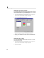
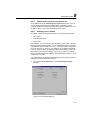
3. Select the Sequence page to display the pre-defined sequence in the
sequence editor field.
4-3
4
Creating methods from method templates
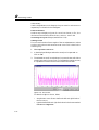
Figure 4-2. Sequence page in Run setup containing the 20 base
sequence pre-defined in the method template.
4. Click on the Create button (see Section 4.3), which fully generates
the method and inserts default variable values. The Save As
dialogue is then displayed. Save the method with the name test20.
The method must be saved before you can make a run. The test20
method will be displayed in the Methods window of the Main
menu.
5. To run the test20 method, follow the instructions detailed in
Section 4.7 and Chapter 6. You can change the method variables
prior to the commencement of the run.
4.3 Creating a sequence and method
As described in Section 4.2, some of the method templates contain a
partially built method for a pre-defined 20 base sequence. These
templates are:
• Fix Column Recycling Coupling
4-4
•
Fix Column Flowthrough Coupling
•
Adj Column Recycling Coupling
•
Adj Column Flowthrough Coupling
Creating methods from method templates
4
By replacing the pre-defined sequence in these method templates with
a sequence of your choice, you can quickly and easily create a readyto-run method.
1. Select a method template in the New Method dialogue box, as
described in Section 4.1.
2. Click on the Run set-up button on the toolbar or select View:Run
setup.
3. Select the Sequence page to display the pre-defined sequence. Select
the pre-defined sequence in the sequence editor and delete it using
the <Delete> key on the keyboard.
4. Enter a new sequence, up to a maximum of 200 bases, in the
sequence editor in the 5´- 3´ direction. Remember that the synthesis
reaction proceeds in the 3´- 5´ direction, so the 3´ base position is
always the first base on the solid support. This base should be
taken from the standard position and should be oxidated.
Use the radio button combinations to select the base type to be
added for each position. You are able to select DNA or RNA,
whether the base is to be oxidated or thiolated, and whether the
base is taken from the standard or modified reagent position.
There are two extra physical reagent positions in OligoPilot II,
labelled X and Y, both in the standard and modified positions. The
extra characters Z and Q are also provided. The available
combinations are as follows:
Radio button combination
Bases as represented on the
screen
DNA, -O(xidated), Standard
DNA, -O(xidated), Modified
DNA, -S (thiolated), Standard
DNA, -S (thiolated), Modified
RNA, -O(xidated), Standard
RNA, -O(xidated), Modified
RNA, -S (thiolated), Standard
RNA, -S (thiolated), Modified
4-5
4
Creating methods from method templates
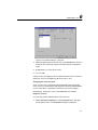
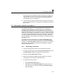
Figure 4-3. Radio buttons in the Sequence page used for choosing the
base type to be included in the sequence.
5. Click on the Group button if you want the sequence to be displayed
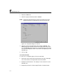
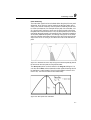
in groups of three bases, beginning from the 5´ end.
Figure 4-4. An ungrouped (top) and grouped (bottom) sequence in the
sequence editor field of the Sequence page.
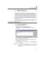
6. To save the sequence you have created, click on the Save As button
and type in a name for your sequence. The name can be up to 256
characters in length. Click on OK. The name of the saved sequence
will now be displayed in the Sequence page containing the specific
sequence. Note that saved sequences are personal to the current
user, i.e. users logged in under a specific username will not see the
saved sequences of another user.
7. Place a check mark in those boxes beside the Optional method
steps that you want to be included in your method.
8. Create the method for the sequence you have entered by clicking
on the Create button. The Create button serves four main
purposes:
4-6
•
to check the sequence for invalid combinations (ignoring the
3´ base), e.g. it is not possible to include both base 'A' (DNA)
and base 'a' (RNA) in the same sequence since they both take
up the same reagent bottle position on the instrument.
•
to generate a method based on the sequence and crossreference list (see Section 5.1.1).
Creating methods from method templates
4
•
update the method variables based on the generated method.
•
display the Save As dialogue so that the method can be saved
before performing a run.
Enter a name for the method, select the destination and click on OK
(see Section 4.6 for more details). The method is saved with default
values for the method variables. These can later be changed before
you start a run (see Section 4.7 and Chapter 6) or you can change
the variables and save the method under a new name.
Note:
Users with the appropriate access authorization have global
access to methods created by all users. In such circumstances,
an already saved method can be used as the basis for
generating a new method with a different sequence. This is
particularly useful if, for example, a method was saved with
specially modified blocks (see Section 5.2) or cross-reference
lists (see Section 5.1.1).
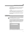
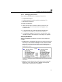
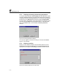
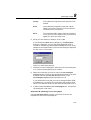
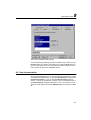
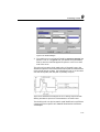
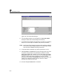
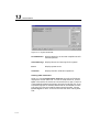
4.4 Editing method variables
The method templates are constructed from blocks representing the
stages in a typical synthesis. Each block has a set of method variables,
displayed on the Variables page in the run setup. You set default values
for the variables in the Method editor, and can change these values for
a particular run in the start protocol before the run is started.
Figure 4-5. The Variables page in Run setup.
4-7
4
Creating methods from method templates
Work through the variable list, adjusting the values to suit your
synthesis. To change a variable value, simply type the required value in
the field. Remember that the values you enter here will be default
values, suggested each time the method is run.
If the whole variable list does not fit on one screen, a scroll bar will be
shown to the right of the list. Click on the arrows at the ends of the bar
to scroll one variable at a time, or on the bar itself to scroll one screen
at a time. You can also drag the slider button to scroll, but this is not
recommended since you can easily miss variables by scrolling too far.
Typical blocks are illustrated with the list below, taken from a method
created for OligoPilot II with the Fix Column Recycling Coupling
template. The list is organised according to the blocks in the method,
with mentioned variable parameters identified in italics. Other method
templates have different structures and variables.
• Start_parameters
These variables together define the synthesis scale, i.e. Weight of the
support, Loading of the support and Column diameter. CV (column
volume) is also defined and is used for the calculation of special
instructions such as Vol_Cap, Vol_amid and CT5_Cap.
• CV_column_wash
The number of column volumes (CV) to wash the column is set here.
If zero is entered, no wash will take place.
• Detrit_peak_start
The flow rate of the detritylation solution is set here.
• Detrit_wash
The pressure of the detritylation wash and the number of column
volumes of detritylation solution to be used are set here.
• DNA_Parameters
These variables together define the coupling of a base to the
oligonucleotide sequence, i.e. how many equivalents of amidite should
be added to the column with respect to the scale, the percentage
volume of tetrazole to be used with respect to column volumes and the
concentration of the amidite.
• DNA_Recycle
The amidite recycling flow rate and time used are set here.
4-8
Creating methods from method templates
4
• Oxidation_DNA
Oxidation stabilizes the phosphite group of the coupled amidite. The
variables determine how many equivalents of iodine are used in the
oxidation solution and the contact time between the oxidation
solution and the support.
• Capping
The unreacted 5´-hydroxyl groups on the oligonucleotide are capped
to prevent further participation in the synthesis reaction. The column
volumes of capping solution and the contact time are set here.
Click on the x-axis button in the graphical display to change a base for
the graphical display. Changing the display base will not affect the
base in the method.
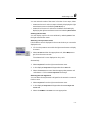
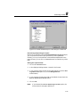
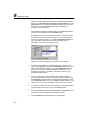
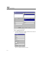
4.5 Method notes
Click on the Notes thumb-tab in the Run setup to show the Notes page,
and read through the method notes. You can maximise each section in
the notes page to fit more of the text on one screen. Click on the printer
icon or choose File:Print to print the method notes.
The method notes provided with each template describe the important
information about the template and, if relevant, how the system should
be connected for the method to work correctly. If your system does not
correspond to the description, either rearrange the valves and tubing
connections in accordance with the method notes description or edit
the method instructions (see Chapter 5) in accordance with your
system setup.
Figure 4-6. The Notes page in Run setup with the method notes maximised.
4-9
4
Creating methods from method templates
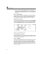
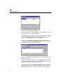
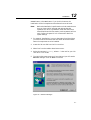
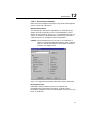
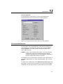
4.6 Saving the method
A new method created from a method template is untitled, and must
be saved under a method name before it can be run. Click on the Save
Method toolbar button or choose File:Save to save the method.
Figure 4-7. Save as dialogue for saving a method.
1. If required, select another folder than the default home folder in
which to save the method.
2. Enter a Method name for the method. Method names may be up to
256 characters long. The method name must be unique for the
chosen system within the folder (see steps 2 and 3).
3. If you have more than one system connected to the computer,
choose the System for which the method is intended. The method
can only be run on the system for which it is saved. Remember that
different systems may have different configurations and control
capabilities.
Note:
Each method is written for a specific strategy. The function of
the method cannot be guaranteed on systems having other
strategies.
4. Choose the Technique for which the method was written.
5. Click on OK.
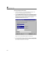
4-10
Creating methods from method templates
Note:
4
The method templates are written for standard strategies. If
you receive a syntax error message when the method is saved,
one or more instructions in the method are invalid. These may
be calls to blocks which are not defined, or instructions which
are invalid in your customised strategy (this can also arise if a
method is written for one system and saved for another).
Invalid instructions are marked in red in text instruction mode
in the Method editor (see Section 5.4.1), and must be deleted
or replaced before the method can be run.
The method remains open in the Method editor when it has been
saved, so that you can continue editing if you wish. Once the method
has been saved, choosing File:Save saves the current state of the
method under the same name. If you want to save a copy of the method
under a new name, choose File:Save As and enter the details as
described above.
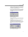
4.7 Starting a run
This section briefly summarises how to start a run with a method. The
method must be named and saved before it can be started. See Chapter
6 for more details of how to run a method.
Note:
If you are editing the method in the Method editor and have
made changes that you have not yet saved, these changes will
not apply during the run. Similarly, if you edit the method
while it is running, the run will not be affected. It is the version
of the method that is saved on disk at the time when the
method is started that controls the run.
1. Establish a control mode connection to the system where the
method is to be run. See Section 6.5 for details. You cannot start a
method without a control mode connection to the appropriate
system.
2. Choose File:Run from System control for the required connection
and select the method to run. Alternatively, click on the method in
the Methods window of the Main menu and select Run from the
right mouse button menu. Do not double-click on the method icon
in the Main menu as this will open the Method editor.
3. Change the method variable values if required. The suggested
values are those saved in the method. Any changes you make will
apply only for the current run, and will be recorded in the run
documentation.
4-11
4
Creating methods from method templates
4. Go through the rest of the Start protocol, entering information
where appropriate. Use the Next and Back buttons to move
through the Start protocol. If you click on Cancel on any page in
the start protocol, the method will remain loaded in the System
control module but will not start. Start protocol pages for most
method templates are:
Variables
Adjust variable values as required for the run.
Questions
Fill in answers to the questions.
Notes
Read the method notes and enter start notes if
required.
Evaluation
Procedures
Oligosynthesis
Sequence
Result
Select the print_chromatogram procedure if you
want the results to be printed automatically.
The sequence of the oligonucleotide to be
synthesized.
Set the result file name and path (folder) as
required. The default result file name includes a
2-digit serial number.
5. The last page of the start protocol has a Start button. Click on this
button to start the run.
4.8 Editing text instructions
Methods for most purposes can be created by adjusting the method
variable values as described above. The method is actually
programmed as a series of instructions that use these variables as
parameters. To see and/or change the instructions, click on the Text
Mode button on the Method editor toolbar or select View:Text
instructions from the menu.
With the Text instruction editor, you have complete facilities for
designing and editing your own customised methods. You will also use
the Text instruction editor for refining and modifying methods based
on the standard templates, e.g.
• Changing the method base (column volume, volume or time).
• Changing valve specifications for inlet and outlet (if the templates
do not suit your system configuration).
4-12
Creating methods from method templates
4
• Adding or removing variables.
• Adding or removing instructions to change the method
functionality.
• Adding or removing blocks to change the method structure.
To gain an understanding of how method templates are built up and
can be modified, work through Chapter 5 which gives a full
description of method editing facilities.
4-13
4
4-14
Creating methods from method templates
Creating and editing methods
5
5
Creating and editing methods
This chapter describes the complete facilities for creating and editing
methods in UNICORN. Refer to Section 2.3 for an overview of
method concepts. For many applications, suitable methods can be
created by changing the default variable values in one of the templates
supplied with UNICORN (see Chapter 4). Use the more advanced
editing facilities described here for:
• changing selected instructions in the method templates, e.g.
changing the outlet valve position
• adding blocks and instructions, e.g. Watch instructions
• changing method instructions to adapt to non-standard system
configurations
• creating new methods for applications which are not covered by
the templates supplied
Advanced editing facilities can be used at three different levels. The
chosen level is dependent on the type and extent of changes to be made:
• modifications at the sequence editor level, i.e. creating custom
methods by assigning a specific base in the sequence editor to a
freely selected block (see Section 5.1).
• adding new blocks to an existing method and/or modifying
instructions in existing blocks (see Section 5.2).
• writing a new method “from scratch”, i.e. selection of No
Template in the New Method dialogue.
5.1 The sequence editor
The sequence editor in the Sequence page of Run setup is a user
interface which allows methods to be easily created. The bases in a
sequence are each cross referenced to a specific block in the method
template, with each block representing a series of instructions to be
performed. Thus, in entering a sequence into the sequence editor and
clicking on the Create button, the specific blocks that are crossreferenced to the bases are copied from the method template into the
method. The method must be saved before it can be then used to run
an instrument.
5-1
5
Creating and editing methods
For example, in a sequence containing the bases 5´-...AC...3´, the DNA
base C is assigned to a specific block in the method template called
Add_DNA_C. Consequently, by clicking on the Create button in the
Sequence page, the C base in the sequence causes the block
Add_DNA_C to be copied into the method. The next base in the
sequence, DNA base A, is assigned to the block name Add_DNA_A.
Thus, the block cross referenced to base A will next be added to the
method (see Figure 5-1). In the standard method templates, each block
that is cross-referenced to a base is a self-contained set of instructions
to perform a complete coupling cycle of one base, i.e. detritylation,
detrit wash, coupling, oxidation or thiolation and capping (see Figure
5-1).
Figure 5-1. The relationship between the bases entered into the sequence
editor and the blocks copied into the method. In the example, the sequence
base C is cross referenced to the block name Add_DNA_C, which is then
copied into the method. Similarly for the following base A, this is cross
referenced to the block named Add_DNA_A which is also copied into the
method. Note that each block contains a self-contained set of instructions for
the complete coupling cycle of the specific base.
5.1.1
Modifying cross references in the sequence editor
Cross referencing a base to a method template block lends much
flexibility to modifying the method creation process. UNICORN OS
allows the user to change the block that is cross-referenced to any
specific base type.
5-2
Creating and editing methods
5
For example, you may decide that the DNA sequence 5´-ACTGGT-3´
should have a column wash step after the addition of each base in the
sequence. By cross referencing a base not used in the current sequence,
e.g. A, to the column wash block in the method template, this can be
directly incorporated into the sequence to signal a column wash. Thus,
in the sequence 5´-AAACATAGAGAT-3´, the appearance of A does
not mean that a thiolated DNA-A base will be added to the
oligonucleotide, but rather a column wash procedure is performed
after the addition of the preceding base.
Alternatively, you may modify the instructions in an existing block or
create a new block. It is thus a straightforward task to assign the new
block to the base in question.
To change the assignment, do the following:
1. Create a new method by clicking on the New Method toolbar
button or choose the File:New:Method menu command in the
Method editor, or by choosing File:New:Method or New:Method in
the Main menu. These alternatives are equivalent. When you
choose the command from the Main menu, the Method editor is
opened automatically. The New Method dialogue box will be
displayed.
2. Choose the system for which the method is intended, e.g.
OligoPilot or OligoProcess. From the Technique pull-down list,
select Any. Next, select one of the available method templates in
the Template pull-down list.
3. Click on OK once you have made your selections. The method
template will now be opened as an untitled method.
4. Click on the Run setup button or select View:Run setup. Select the
Sequence page.
5. Click on the Cross references button to display the Cross
reference list dialogue.
Select the Coupling list tag from the available List field. In the
Block field you will see the all the bases and the block name that
each is cross referenced to in the method template. For example:
A = Add_DNA_A
5-3
5
Creating and editing methods
Figure 5-2. Cross reference list dialogue box.
6. To change the assignment of a base to a different block in the
method template, first select the base in the Block field. Next, click
on the Block pull-down list and select the method template block
that you want assigned to the selected base. The base in the Block
field will now be associated with the block name that you chose.
Figure 5-3. In the above example, the base A has been cross referenced
to the block Column_wash.
5-4
Creating and editing methods
5
You can select any block contained in the method template, even
those that you have modified or created (see Section 5.3). Repeat
this process for other bases as appropriate.
7. You can also reassign the cross references for the optional method
steps selected in the Sequence page. The blocks for Column wash,
Final detritylation, Purge Amidite, and Purge Solvent can be
assigned by clicking on the appropriate tab and then using the
Block pull down list.
Figure 5-4. Fields for cross referencing the column wash and final
detritylation blocks in a method.
7. Click on Exit to implement the new cross references.
8. Enter the appropriate sequence in the sequence editor field of the
Sequence page. Create a method as described in Section 4.2.
9. Save the method (see Section 4.6).
Users with the appropriate access authorization have global access
to methods created by all users. In such circumstances, an already
saved method can be used as the basis for generating a new method
with a different sequence. This is particularly useful if, for
example, a method was previously saved with a specially modified
cross-reference list. In such circumstances, open the appropriate
method containing modified cross-reference list and access the
Sequence page in Run setup. Delete the existing sequence in the
sequence editor and enter the new sequence. Click on the Create
button.
5-5
5
Creating and editing methods
Note:
Do not open a saved sequence from your personal sequence
list in the Sequence page, otherwise the cross-reference list
corresponding to the saved sequence will replace the
modified cross-reference list present in the current method.
Always manually enter your sequence over the original
method sequence.
5.2 Text instruction editor
The next level of advanced editing to create new methods uses Text
instructions. This involves modifying the instructions within the blocks
of an existing method and/or adding new blocks to methods.
Note:
Users with the appropriate access authorization have global
access to methods created by all users. In such
circumstances, an existing method can be used as the basis
for generating a new method with a different sequence. This
is particularly useful if, for example, a method was
previously saved with specially modified blocks.
This section introduces you to the Text instruction editor and the
following sections present the components of a method and how to
edit and create blocks.
The text instruction editor is used for entering and editing method
instructions. Click on the Text instructions toolbar button or choose
View:Text Instructions to display the text instruction editor.
Figure 5-5. The Method editor in text instruction mode, showing the Block
window (top), text instruction window (centre) and instruction box (bottom).
5-6
Creating and editing methods
5
Up to four windows can be displayed together with the instruction
box. Click on the View Windows toolbar button or choose the
View:Windows menu command to open a dialogue for choosing which
windows to display.
Figure 5-6. The Windows dialogue for selecting which windows to display in
the Method editor.
Method editing operations which can be performed in the various
windows are summarised in the table below.
Window
Operations
See Section
Text window
Display and hide block
instructions. Select current
instruction. Move instructions
within a breakpoint.
5.4
Flow scheme window
For information only. The
flow scheme picture is static
and is therefore not updated
according to system status or
changes in the method.
5.4.5
Instruction box
Specify breakpoints, instructions, parameters and variables. Insert, change and delete
instructions.
5.4.2 5.4.4
5-7
5
Creating and editing methods
5.2.1
Run setup
The Run setup is a series of pages for defining the method properties.
To access the Run setup pages, press the Run setup toolbar button or
select View:Run Setup from the menu.
Figure 5-7. Run setup with the Variables page displayed.
To access a given page in the Run setup, click on the relevant tab. Pages
in the Run setup editor are described in Section 5.6.
5.3 Method blocks
Viewing a method as a long list of individual text instructions would
be confusing and inconvenient. Text instructions are therefore
conveniently grouped into blocks of instructions that define a specific
functional use. For example, one block might contain the instructions
necessary for equilibrating a column, and another block contain
instructions for adding a single defined nucleotide in the sequence, etc.
By using such blocks it is easier to build up a total method for a run.
5.3.1
Viewing blocks
It is possible for one block to contain one or several other blocks. This
is most evident, for example, in the Text instruction window.
5-8
Creating and editing methods
5
In the text instruction window
In the text instruction window, the method is shown as a list of blocks,
denoted by the blue square symbols. Beside each block is also a ‘+’
symbol, which you can click on to expand the view of the instructions
within the block. Note that a block can also contain other blocks as
denoted by the blue square symbols.
Unexpanded
blocks in a method
Expanded block in a
method containing
text instructions and
blocks.
Figure 5-8. Text instructions showing blocks in a method.
To collapse the view, click instead on the ‘-’ symbol for that block.
Alternatively you can double click on the block name to view or hide
the instructions (see Section 5.4.1).
In the block window
The organisation of blocks in the method is shown graphically in the
block window in text instruction mode.
Each block is represented by a grey bar with the block name and the
length of the block. The line is shifted down to indicate calls to other
blocks. In the example below, the blocks are called in sequence from
the Main block at breakpoint 0. Blocks to which there is no valid call
are not shown in this window.
5-9
5
Creating and editing methods
Figure 5-9. The Method editor block window.
Conditional (Watch) instructions are indicated by a green line showing
the start and duration of the watch. The example above has a Watch
instruction to start the fraction collector which is active throughout the
gradient elution block. Loop instructions (to repeat a group of
instructions) are also indicated in the block window.
If you click on the line representing a block in the block window, the
first instruction in the block will be highlighted in the text window.
5.3.2
Calling blocks
To execute the instructions contained within a block in a method, the
block must be called by the program. When a block is called the
instructions in the block are executed in the order that they are written
until the block is finished or the End_Block instruction is executed.
Any settings made in a block are valid throughout the method until the
settings are changed.
Figure 5-10. Illustration of the flow of process control through method blocks.
5-10
Creating and editing methods
5
Calls may be of two types:
• Unconditional calls are made with the Block instruction.
• Conditional calls are made with a Watch instruction, which makes
it possible to call a specified block or an instruction when a
particular monitor signal meets a given condition. As long as the
condition is not met, the block is not activated. There are different
Watch instructions for each process monitor signal, and each
Watch instruction can use various conditions to respond to
absolute signal values or to rate of signal change.
Note that the breakpoint when the Watch instruction is issued
determines when the watch begins, not when the block is
activated. The block will in fact never be activated if the watch
condition is not met during the run.
Once set, a watch remains active until the condition is met or a
new Watch instruction is issued for the same monitor. The watch
is cancelled automatically when the condition is met. A watch can
also be turned off with the Watch_off instruction.
See Section 5.8.7 for more details of Watch instructions.
5.3.3
Adding blocks
To add a new block use the Text instruction editor and click on the
New block toolbar button or select Block:New.
Figure 5-11. New block dialogue.
5-11
5
Creating and editing methods
Alternatively you can enter the Block instruction in the Instruction
box, enter a name for the block in the parameter field and click on
Insert.
Block name
Enter a name for the block in the Name field. Block names may be up
to 30 characters long, and may contain letters (A-Z), digits (0-9) and
underscore characters.
Block names must be unique within the method. The case of letters is
retained but is not significant (the names Add_DNA_W and
add_dna_w are treated as identical).
Base
Choose a base for the block. If you choose SameAsMain, the new block
will inherit the base from the Main block in the method. The
corresponding Base instruction will be inserted in the block at
breakpoint 0. If you choose CV, enter a value for the column volume.
If you chose a specific column, a column volume is entered
automatically.
Length
You can enter a length for the block if required. An End_Block
instruction will automatically be inserted in the block at the
corresponding breakpoint. This field may not be left blank.
Call
You can call the new block from an existing block (e.g. the Main
block). The block is called by an instruction named Block. Choose the
block from which the newly created block should be called in the From
field and enter the breakpoint at which the call is to be made in the At
field. If you do not want to call the block (e.g. when the block being
created is to be activated by a Watch instruction), choose an empty line
in the From field. These blocks are placed last in the method in the
Unused category.
Note 1: If the Block instruction is placed at the same breakpoint as
the End_Block instruction, the Block instruction will be
placed immediately before End_Block.
Note 2: Do not call a block from within itself. You will generate a
potentially infinite loop, which exceeds the maximum
number of calls allowed in a method. A loop symbol is
displayed at the beginning of the line if this occurs.
Press OK to add the new block.
5-12
Creating and editing methods
5
Strategy for creating blocks
For blocks which are to be called unconditionally, you have the option
of creating the Block instruction at the same time as you create the
block, by selecting where the block will be inserted in the From field of
the New block dialogue.
For blocks which are to be called conditionally with a Watch
instruction, first create the block and save it under unused by selecting
an empty line in the From field. Insert the Watch instruction into the
text method and then make a call to the block. The block will move
from unused to beneath the Watch instruction.
Note:
If you call the block before inserting the Watch instruction,
a copy of the block will be created, i.e. there will be two
instances of the block in the text method.
5.3.4
Deleting blocks
To delete a block from the method using the right mouse button menu:
1. Click on the desired block in the method with the right mouse
button to display the menu.
2. Select Delete. A warning dialogue is displayed requesting if you
want to totally delete the block instruction from the method.
Answer as appropriate:
Yes The block is totally removed from the method. Blocks deleted
in this fashion can not be called again in the
method.
No The block is deleted from the method and transferred the
Unused line. Blocks deleted in this fashion
can be called again in the method.
To delete a block from the method using the Block:Delete command:
1. Select the menu command Block:Delete. The Delete block dialogue
is displayed with all blocks listed in alphabetical order.
2. Select the block to be deleted and click on Delete.
3.
A warning dialogue is displayed requesting if you want to totally
delete the block instruction from the method. Answer Yes or No as
described for this function using the right mouse button menu
command (above)
5-13
5
Creating and editing methods
5.3.5
Renaming blocks
To rename blocks, choose Block:Rename Block or select a block in the
method using the right mouse button and select Rename from the
menu. In both instances the Rename blocks dialogue is displayed.
Figure 5-12. The Rename Blocks dialogue
By default, the block that is currently highlighted in the method text
instructions is automatically selected in the dialogue. Enter the new
name in the New Name field and press Rename. The dialogue remains
open until you press Close, so that you can rename more than one
block without closing the dialogue.
If the block you renamed is used in a Block or Watch instruction, the
block name in these instructions will be changed automatically.
5.3.6
Copying, moving and importing blocks
You can copy, cut and paste blocks within a method or import blocks
from another method.
Copying blocks
To copy blocks within a method:
1. Select the block to be copied using the right mouse button. Select
Copy from the menu.
2. Select the instruction line before which you want the copied block
to be pasted.
5-14
Creating and editing methods
5
3. Click on the right mouse button and select Paste from the menu.
A dialogue requests if you wish to rename the pasted block. Click
on Yes to rename the block before insertion or No to directly insert
the copied block.
The pasted block is inserted with the same breakpoint value as the
block selected for point of insertion.
Cutting and pasting blocks
To cut and paste blocks within a method:
1. Select the block to be copied using the right mouse button. Select
Cut from the menu. The block is removed from the text instruction
window.
Note:
A cut block does not mean that it has been deleted (see
Section (5.3.4) and can still be called from elsewhere in the
method.
2. Select the instruction line before which you want the cut block to
be pasted.
3. Click on the right mouse button and select Paste from the menu.
The pasted block is inserted with the same breakpoint value as the
block selected for point of insertion.
Importing blocks
Blocks may be imported from other method files to which you have
access including the current method file in which you are working.
1. Select Block:Import Block As.
2. Choose the method from which you wish to import and mark the
block to import. The name of the selected block is suggested in the
Block name field.
3. Select a block from the Call drop-down list into which the
imported block will be placed and enter a breakpoint value.
4. Click on Import to import the block. The dialogue remains open
until you click on Close, so that you can import more than one
block without closing the dialogue.
5-15
5
Creating and editing methods
Note:
If you use the import function to copy blocks within a
method, the blocks are copied from the saved version of the
method on disk. Any changes you have made in the method
but not yet saved will not be copied.
The imported block may not have the same name as an existing
block in the method. If the default name is not allowed for this
reason, the Import button will be grey and locked. Change the
name of the imported block so that the Import button becomes
available.
The block is imported exactly as it appears in the source method.
If the base of the imported block is defined as SameAsMain, the
block will inherit the main base in the new method, regardless of
the base in the source method. Also, the pasted block is inserted
with the same breakpoint value as the block selected for point of
insertion.
Figure 5-13. The Import Block dialogue.
5-16
Creating and editing methods
5
5.4 Method instructions
Use the Instruction box in text instruction mode to enter, edit and
delete instructions.
5.4.1
Viewing instructions
Instructions are displayed in the text Instruction box.
Figure 5-14. The text instruction window (top) with the instruction box
(bottom).
Instructions are displayed in the text instruction window as follows:
Blue square beside text
Valid call instructions (i.e. Block and
Watch instructions to other blocks in the
method).
Bold text
Valid instructions.
5-17
5
Creating and editing methods
Red bullet beside text
Instructions with invalid syntax. These
may be: (a) calls to blocks which are not
defined in the method, or (b) instructions
which apply to a different system strategy
(these can arise if a method is written for
one system and saved for another). All such
instructions must be deleted or changed
before a method can be run (see Sections
5.4.3 and 5.4.4).
Normal text
Instructions which will not be executed
because they are either after the end of a
block or method or constitute a block to
which there is no call.
Text with a loop symbol
When a block is called from within itself
this will generate a potentially infinite loop,
which might exceed the maximum number
of calls allowed in a method.
Double-click on a Block or Watch instruction to display or hide the
instructions in the called block or click on the ‘+’/’-’ symbol for the
block respectively. Double-clicking on the Main keyword at the
beginning of the method will show or hide instructions in all blocks in
the method.
Figure 5-15. Displaying and hiding block instructions.
General oligosynthesis instructions are listed in Appendix B.
5-18
Creating and editing methods
5.4.2
5
Adding instructions
To add a new instruction:
1. In the text instruction window, select an appropriate block and
display the instructions within the block.
2. Select an instruction line in the block.
Figure 5-16. Instructions added at the same breakpoint as existing
instructions are inserted after the highlight.
Note:
Make sure that the selected instruction line is within the
block, not the call to the block.
3. New instructions are added from the Instruction box. Open the
Instruction box if not already displayed (View:Windows). For the
new instruction:
(a) Set the desired breakpoint in the Breakpoint field.
(b) Choose the instruction type from the five or six options,
depending on the strategy, and select the desired instruction
from the displayed list. For short help on the purpose of each
instruction, click on the instruction and press <F1>.
(c) Enter values for instruction parameters in the Parameters field.
If a scroll bar appears on the right-hand side of the Parameters
field, additional parameters are required.
Figure 5-17. The Method editor Instruction box.
5-19
5
Creating and editing methods
4. Click on Insert. The new instruction will be inserted in the block
either
(a) at the position of the breakpoint of the new instruction if there
are no other instructions at that breakpoint
(b) immediately after the currently highlighted instruction if the
highlight is at the same breakpoint as the new instruction
(c) as the last instruction at the breakpoint if there are several
instructions at the same breakpoint as the new instruction and
none of these is highlighted.
Note:
Instructions that are placed at the same breakpoint are
executed simultaneously, with the exception of Block
instructions which are executed in the sequence in which
they are written.
5.4.3
Deleting instructions
To remove an instruction:
1. Select the instruction in the text instruction window.
2. Press Delete in the Instruction Box, or press on the <Delete> key,
or click on the right mouse button and select Delete.
An instruction that has been deleted can only be recovered by reinserting the instruction. If you want to suspend execution of an
instruction temporarily (e.g. during development work), you can
replace the breakpoint with a value after the End_block or
End_method instruction. Any instructions after the end of a block or
method will not be executed.
Note:
You cannot delete the Base instruction at the beginning of a
block.
Caution: If you delete the End_block instruction, the block will end at
the last instruction in the block.
5-20
Creating and editing methods
5.4.4
5
Changing instructions
There are three possibilities for changing an instruction:
• change the breakpoint
• change parameters (including variables, see Section 5.5)
• select another instruction
To change an instruction:
1. Select the instruction in the text instruction window. The
instruction with its current parameters will appear in the
Instruction Box.
2. In the Instruction Box, make the required changes to the
breakpoint or parameters or choose a new instruction.
3. Press Change or Replace. These buttons are equivalent unless
changes are made to the breakpoint or the length of a gradient
Changing breakpoints
Change and Replace have different functions if the breakpoint is
changed:
• Change shifts all subsequent instructions in the block according to
the change in the breakpoint. Change does not affect the relative
order of instructions in the method. You cannot change the
breakpoint of an instruction to earlier than the nearest previous
breakpoint in block.
Figure 5-18. Change moves the selected instruction and all subsequent
instructions.
• Replace moves the selected instruction but does not change the
breakpoint of any other instruction. Replace can change the
relative order of instructions in the method:
5-21
5
Creating and editing methods
Figure 5-19. Replace moves only the selected instruction.
Moving instructions within a breakpoint
To change the order of instructions within the same breakpoint in a
block, mark the instruction to move with the left mouse button and
drag the instruction to its new location, holding the left mouse button
down. You can only move instructions in this way within a group of
instructions at the same breakpoint.
Figure 5-20. Instructions can be moved within the same breakpoint by
dragging with the right mouse button.
Moving instructions between breakpoints
To move an instruction to another breakpoint:
1. Select the block to be moved using the right mouse button. Select
Cut from the menu. The block is removed from the text instruction
window.
Note:
A cut block does not mean that it has been deleted (see
Section (5.3.4) and can still be called from elsewhere in the
method.
2. Select the instruction line before which you want the cut block to
be pasted.
5-22
Creating and editing methods
5
3. Click on the right mouse button and select Paste from the menu.
The pasted block is inserted with the same breakpoint value as the
block selected for point of insertion.
5.4.5
The flow scheme window
The flow scheme window displays the configuration of system
components. This window is static and for information only, useful for
example in identifying valves for flow path instructions.
Figure 5-21. The Method editor flow scheme window.
5.5 Method variables
Variables can be assigned to many instruction parameters even
including breakpoints. Variable values can be changed immediately
before the start of a run without using the Method editor, allowing one
method to be used for runs under a variety of conditions (see Chapter
4).
Variables are defined with names which can be explicit descriptions of
the variable function, e.g. Sample_volume, Load_of_support. Suitable
choice of variable names can make the method easier to read and
understand, and also help the operator in setting variable values at the
start of a run.
Each parameter defined as a variable is also assigned a default value,
which is used if no changes are made to variable values at the start of
a run. Up to 64 variables can be defined in a single method.
5-23
5
Creating and editing methods
5.5.1
Identifying variables
Parameters defined as variables are identified in two ways:
• in the text instruction window, the parameter is given as the
default value in parentheses followed by the variable name, e.g.
(3.00)#Recycle_Time_DNA Recyle 0.00{cm/h}, OFF.
Figure 5-22. Default values for variables appear in parentheses in Text
instructions
• when the instruction is shown in the Instruction box, the VAR
button beside the parameter field is active in capital letters, i.e.
VAR not Var.
Figure 5-23. Parameters with variable definition are identified by an active
(not greyed out) VAR button. In this example the Watch Efficiency Value is
defined as variable and the Action position is fixed.
All variables are also listed on the Variables page of the Run setup (see
Section 5.6.1), grouped according to the block in which they appear.
5.5.2
Defining variables
To define a new variable (i.e. convert an existing fixed value to a
variable):
1. In the Text instructions window, select the instruction where you
want to define the variable. The parameters for the instruction are
shown in the instruction box.
2. Locate the breakpoint or the required parameter in the instruction
box. Click on the Var button.
5-24
Creating and editing methods
5
3. Enter a name for the variable in the dialogue and click on OK.
Figure 5-24. The Variable name definition dialogue.
Variable names may be up to 20 characters long, and may contain
letters (A-Z), digits (0-9) and the underscore character. Use
underscore characters instead of spaces if you want to separate
words in a name (e.g. Flow_rate). Names must be unique within
the method.
The case of letters is retained but is not significant. The names
Flow_Rate and FLOW_RATE are treated as identical.
When you define a variable, the value in the parameter field applies
as the default value for the variable.
Note:
Only one variable which affects block length (breakpoint or
gradient length) may be defined within each block. Any
number of other parameters may however be defined as
variables within a block.
Figure 5-25. Relationship between variables in text instructions and in the
Variables page of Run setup.
Default variable values can be changed either by editing the instruction
in the Instruction box or by changing the value in the Variables page
of Run setup. Changes made in the text instruction are automatically
updated in the Variables page and vice versa (Figure 5.26).
5-25
5
Creating and editing methods
Caution: If a breakpoint is defined as a variable, changing the variable
value when the method is started will shift other instruction
breakpoints accordingly. This functionality is equivalent to
using Change to alter a breakpoint or gradient length.
5.5.3
Removing a variable
To convert a variable to a fixed value:
1. In the text instruction window, select the instruction where you
want to remove the variable. The parameters for the instruction
will be shown in the instruction box.
2. Locate the required parameter in the Instruction box. Press the
VAR button.
3. Click on Clear to delete the variable name and click on OK.
5.5.4
Renaming a variable
To change the name of an existing variable:
1. In the Text instruction window, select the instruction where you
want to rename the variable. The parameters for the instruction
will be shown in the instruction box.
2. Locate the required parameter in the instruction box. Press the
VAR button.
3. Enter a new variable name in the dialogue and click on OK.
5.6 Run setup
The Run setup is a series of pages for defining the method properties.
To access the Run setup pages, press the Run setup icon at the top of
the Method editor toolbar. To access a given page in the Run setup,
click on the respective tab.
5.6.1
Variables
The Variables page lists all variables used in the method with their
default values, organised by method block. You can change the default
values to create a variant of the method (see Chapter 4).
5-26
Creating and editing methods
5
Figure 5-26. The Variables page in Run setup.
To change the default values, simply enter new values in the
appropriate fields. Use the scroll bar to display additional variables if
the variables occupy more than one screen. Click in the scroll bar to
move one screen at a time, or on the arrows to move one variable at a
time.
The changed values will be displayed for the corresponding
instructions in the text instruction window. Remember to save the
method with the changed variables.
Note:
The Variables box must be checked in the Start protocol if
you want to be able to change variable values at the start of
a method.
5.6.2
Questions
Questions provide a means for entering structured run-specific
information at the start of a run. Method templates supplied with
UNICORN are defined with a set of questions for sample, column and
eluent identification. To define questions which will be shown when
the method is started, open the Questions page in Run setup.
Note:
For questions to be shown in the start protocol, the
Questions option must be checked in the Run set up Start
Protocol page.
5-27
5
Creating and editing methods
Questions may have the following status:
• Mandatory: these questions must be answered before a method is
started.
• Authorised: answers to these questions must be acknowledged by
a user with Confirm/Unlock authorisation (see Section 14.2). The
user's password must be given to acknowledge the answers.
• Chromatogram: these questions will be printed with the answers
on the same page as the chromatogram if Diagram header is
chosen in an evaluation report (see Section 9.5).
Figure 5-27. The Questions page in Run setup
Questions may be defined to accept four types of answers:
• Input field accepts any alphanumerical input as the answer. Input
field questions may have a default answer. Example
Figure 5-28. Options for input field questions.
5-28
Creating and editing methods
5
• Multiple choice allows the user to choose one of a defined set of
answers. To allow a blank answer, enter a space in one of the predefined answers. Example:
Figure 5-29. Options for multiple choice questions.
• No answer does not require an answer. This kind of "question"
may be to display important information or to split a question
over more than one line (by setting all but the last line to No
answer). Example:
Figure 5-30. Options for no answer questions.
5-29
5
Creating and editing methods
• Value accepts only numerical answers. Value questions may have
specified maximum and minimum limits, and may be defined to
accept only integer values.
Figure 5-31. Options for value questions.
Press the Preview button to display the questions as they will appear
when the method is run. (Alternative answers to multiple choice
questions are not shown in this mode). From preview mode, press Edit
to return to question editing mode.
Inserting a question
To insert a new question after an existing question:
1. Click on the existing question in the questions list.
2. Enter the text, status, type and answer for the new question as
required. The Answer panel depends on the type of question:
•
Input field questions: Enter a default answer if required.
•
Multiple choice questions: Click on the input field under
Alternatives, enter the answer and click on Add/Delete.
Repeat this procedure to add other alternatives. New
alternatives are always added at the end of the list. To remove
an alternative, mark the alternative in the scroll list and click
on Add/Delete.
•
Value questions: Enter maximum and minimum limits. Check
the Integer box to if the question is to accept only whole
numbers as answers.
3. Click on Insert to add the new question to the list.
If the list is empty, the Insert operation creates the first question in
the list.
5-30
Creating and editing methods
5
Editing an existing question
To change the definition of an existing question, select the question to
be changed. Change the text, status, type and answer as required and
click on Replace.
Deleting a question
To remove a question, select the question and click on Delete. To
remove all questions, click on Delete All.
5.6.3
Notes
Notes are descriptive comments that form part of the method
documentation. There are four separate notes fields for method
editing, start-up, run and evaluation respectively. Only the method
notes can be edited from the Method editor: the other notes are
accessible at the respective stages in a run.
To view the method notes, open the Notes page in the Run setup.
Method templates are supplied with notes describing the system
requirements for running the method. Read through these notes
carefully before using a method. Click on the maximize notes button
to expand a notes field to fill the notes page. Click on the same button
again to restore the default display with all four notes fields visible.
Figure 5-32. The Notes page in Run setup.
5-31
5
Creating and editing methods
The notes are entered as free text and may be edited using standard
Window editing functions to edit the notes. Words wrap automatically
at the end of the field.
<Ctrl+X>
Cuts the marked text, saving it to the clipboard.
<Ctrl+C>
Copies the marked text to the clipboard.
<Ctrl+V>
Pastes the contents of the clipboard at the
cursor.
<Delete>
Clears the marked text without saving it in the
clipboard, or deletes the character to the right of
the cursor if no text is marked.
<Backspace>
Clears the marked text without saving it in the
clipboard, or deletes the character to the left of
the cursor if no text is marked.
In the default method templates supplied with UNICORN, the method
notes describe the system setup required by the method (e.g. eluent and
sample inlets, outlets, column connections and so on). We recommend
that you use method notes for this purpose in your own methods, to
provide documentation of the method requirements. Bear in mind that
method notes are saved with the method and apply to all runs made
with the method. Use the start or run notes for run-specific
information. The date and time when the method was created and last
edited are saved automatically in the method information, and need
not be entered in the method notes.
5.6.4
Evaluation procedures
Evaluation procedures can be called automatically at the end of a
method to evaluate and/or print the results. Method templates
supplied with UNICORN include procedures named:
Integrate_and_Print which integrates the first UV curve in the
chromatogram and prints out the results
Print_Chromatogram which prints the chromatogram from the run
with the scouting variables printed at the top.
User-defined procedures are created in the evaluation module and may
be saved in method files (see Section 10.3). Procedures saved with one
method file can be imported to another.
5-32
Creating and editing methods
5
Note 1: A procedure in a method will not be updated when a
procedure with the same name is changed in Evaluation. The
same applies to report formats saved in a procedure.
Note 2: If you use an evaluation procedure to print results
automatically from a run controlled from a remote station in
a network installation, the results will be printed on the
printer currently set up on the local station, not on the
remote station. If however you execute the procedure
interactively from the evaluation module on the remote
station, the results will be printed on the printer set up on the
remote station where you are working.
Figure 5-33. The Evaluation Procedures page in Run setup.
Defining and viewing procedures
Evaluation procedures are normally defined in the Evaluation module.
Procedures imported to a method can also be viewed and edited in the
Method editor; select the required procedure in the list and click on
Edit. See Section 10.3.2 for a description of how to edit evaluation
procedures.
Note:
Evaluation procedures which process chromatogram data
rely on consistent identification of curves in the result file for
correct operation. If you include evaluation procedures with
a method, make sure that references to curves in the
procedure will be valid when the procedure is executed at the
end of the run. See Section 10.3 for more details.
5-33
5
Creating and editing methods
Selecting procedures to run
The Evaluation Procedures page lists all evaluation procedures
associated with the method. Click on the procedure(s) which are to be
executed at the end of the run. The procedures will be executed in the
order they appear in the list.
Importing procedures
To import an evaluation procedure:
1. Select the Evaluation Procedures page and click on Import.
2. Choose a procedure from the Select list. You can also choose to
import a procedure from another method. Select a method to show
the procedures stored in the method. If you have chosen a method,
click on Evaluation Procedures to return to the complete list.
3. If desired, change the procedure name in the Import as field.
4. Click on Import.
The dialogue remains open until you click on Close, so that you
can continue to add procedures from the same or different method
files.
Figure 5-34. The Import procedures dialogue.
5-34
Creating and editing methods
5
Deleting procedures
To remove one or more procedures from the method:
1. Select the Evaluation Procedures page and select the procedure(s)
to be deleted.
2. Click on Delete and confirm the deletion.
Note:
Procedures that you delete from the method are removed
from the method file when you save the method.
Renaming procedures
To rename a procedure in a method:
1. Select the Evaluation Procedures page and click on Rename.
2. Select a procedure from the list and change the name in the
Rename item to field.
3. Click on Rename.
The dialogue remains open until you click on Close, so that you can
rename more than one procedure without closing the dialogue.
Editing procedures
To edit a procedure in a method:
1. Select a procedure on the Evaluation Procedures page and click on
Edit.
2. Edit the procedure as described in Section 10.3.
3. Choose File:Exit from the procedure editor menu. (File:Save is not
available in the procedure editor window when you edit
procedures in a method. Changes are saved automatically when
you close the procedure editor).
Note:
Report formats in procedures cannot be edited or viewed.
5-35
5
Creating and editing methods
5.6.5
Method Information
Figure 5-35. The Method Information page in Run setup.
The Method Information page displays information about the method,
such as method name, target system for creation and date of last
change, information about the strategy for which the method was
created, estimated eluent consumption and duration in time of the
method. These figures for the latter two are based on values for
methods with variable length parameters, and will be changed if the
values are changed.
The Method Information page is for information only and cannot be
edited.
5.6.6
Sequence
The Sequence page contains the user interface between the desired
sequence to be synthesized and the method created to run the synthesis
procedure. The properties of this interface are described in Chapter 4
and Section 5.1.
5.6.7
Result Name
Use the Result Name page to specify how the result files will be named
for the results of a run, and where the result file will be saved.
5-36
Creating and editing methods
5
Figure 5-36. The Result Name page in Run setup.
The result file name is constructed by adding a 2-digit serial number to
one of the base options listed below. The serial number is incremented
automatically each time the method is run.
• the method name plus a 2-digit serial number
• the date of the run (in an 8-digit format determined by the country
setting in Windows NT) plus a 2-digit serial number
• a freely specified name (within the file naming restrictions in the
operating system) plus a 2-digit serial number
If the result file folder already contains files with the same file name
base, the serial number is incremented automatically.
By default, result files are stored in the home folder of the user who
starts the run. To change the folder where the result file will be stored,
press the Browse button, double-click on the required folder icon and
press Close.
Note:
The result name may be specified as changeable in the Start
protocol (see Section 5.6.10). In that case, the specification
in the Result page serves to generate the suggested result
name, which may be changed at the start of the run.
5-37
5
Creating and editing methods
5.6.8
Start protocol
The Start protocol determines which items of the Run setup are
displayed (and may in appropriate cases be altered) at the start of a
run. Open the Start Protocol page and check the items that are to be
displayed.
Figure 5-37. The Start Protocol page in Run setup.
Variables
If this box is checked, values for method variables will be displayed
and can be changed at the start of the run. These values will override
the default values for the particular run, and will be saved in the result
file. The default values stored in the method are however not affected.
If the Variables box is not checked, the run will be executed with
default values for all variables as defined in the method.
Text Method
Displays the method instructions. Double-click on a Block instruction,
as denoted by the blue square and ‘+’ mark, to display or hide the
instructions in the called block (see Section 5.4.1). Method instructions
cannot be changed from this display.
Questions
If this box is checked, questions defined in the method will be
displayed at the start of the run.
5-38
Creating and editing methods
5
Important!
If the Questions box is not checked, questions will not be displayed
even if they are defined as mandatory. Since the answers to questions
can form an important part of the run documentation, you are
recommended always to check the Questions box.
Notes
If this box is checked, the notes page will be displayed at the start of
the run. You can enter notes in the Start notes field but not in any of
the other fields. You can use the scroll bar if necessary to read notes in
the Method notes field.
The start of the run is the only occasion when you can enter start notes.
If the Notes box is not checked, the notes will not be displayed and you
cannot enter start notes for the run.
Columns
If this box is checked, you can view the available column definitions.
The column definition used in the method run is selected with the Base
instruction, and may be changed at the beginning of the run on the
Variables page if the columns parameter is defined as a variable (see
Section 5.6.1).
Note:
Not used for Oligo systems.
Reference curves
If this box is checked, the reference curves associated with the method
will be displayed at the start of the run. You can add, delete and
rename curves at the start of the method. All curves in the list can be
displayed in System control during the run.
If the Reference curves box is not checked, the curve settings saved in
the method will apply.
Evaluation procedures
If this box is checked, the evaluation procedures set to execute at the
end of the method will be displayed at the start of the run. You can
change the choice of procedures to execute, but you cannot add or
remove procedures. (Procedures are stored as part of the method file,
which cannot be changed at the start of the run).
If the Evaluation Procedures box is not checked, the procedure settings
saved in the method will apply at the end of the method.
5-39
5
Creating and editing methods
Method information
If this box is checked, the method information (including creator,
target system, strategy information and date and time of creation and
latest change) will be displayed at the start of the run. You cannot edit
the method information.
Settings
If this box is checked, the settings (including alarms, monitors and
curve configuration) will be displayed for information at the start of
the run.
To change settings, use the System:Settings command in System
control before starting the run (see Chapter 15).
Calibration
If this box is checked, the monitor calibration settings will be displayed
at the start of the run.
If the Calibration box is not checked, you can still calibrate the
monitors before the run is started by using the System:Calibrate
command in System control.
Result name changeable
If this box is checked, you can change the result name when the run is
started. Click on the Browse button to change the result folder.
If the Result name changeable box is not checked, the result name will
still be displayed, but neither the name nor the folder can be changed.
Sequence
This option should be selected to display the sequence that the method
has been created for. This is for information only.
5.7 Saving the method
5.7.1
Saving a method
Click on the Save button on the toolbar or choose File:Save to save the
method. The method remains open in the Method editor when it has
been saved, so that you can continue editing if you wish. Once the
method has been saved, choosing File:Save saves the current state of
the method under the same name. If you want to save a copy of the
5-40
Creating and editing methods
5
method under a new name, choose File:Save As and enter the details
as described below.
1. Enter a name for the method. Method names may contain letters
(A-Z) and digits (0-9). The case of letters is not significant. The
method name must be unique for the chosen system within the
folder (see steps 2 and 3 below).
2. By default, the method will be saved in your home folder. To
change the folder, double-click on the appropriate folder icon in
the Methods panel.
Figure 5-38. Save As dialogue for saving a method.
3. If you have more than one system available, choose the system for
which the method is intended. The method can only be run on the
system for which it is saved. Remember that different systems may
have different configurations and control capabilities.
Note:
Each method is written for a specific strategy. The function
of the method cannot be guaranteed on systems having other
strategies.
4. Click on OK.
5.7.2
Saving as a template
You can save the method as a template if you have Edit global lists
authorisation.
1. Choose File:Save as Template. The Save As Template dialogue is
displayed.
5-41
5
Creating and editing methods
2. Enter a name for the template in the Name field, or choose an
existing template name from the list. If you choose an existing
name your will overwrite the existing template.
3. Choose the system for which the template is intended in the For
system field.
4. Select the Technique from the lists as appropriate.
5. Click on OK.
The templates for each system are common for all users. Be restrictive
in saving methods as templates. We recommend that only methods
that are useful for all users are saved as templates.
5.7.3
Deleting a template
You can delete templates if you have Edit global lists authorisation.
1. Choose File:Delete template.
2. Select the system and the template to delete, and click on Delete.
3. Confirm the action.
Note:
The templates for each system are common for all users. Be
restrictive in deleting templates.
5.8 Printing the method
You can print a copy of the method including items from the method
documentation (Run setup) and the Text instructions window.
1. In the Method editor select File:Print or click on the Print toolbar
button.
The Print dialogue is displayed. The dialogue contains print
UNICORN modules although only those available from Method
editor can be selected.
Note:
5-42
It is recommended that you select the print command from
the text instructions view so that you have access to the text
method print options.
Creating and editing methods
5
Figure 5-39. Print dialogue
2. Check the options that you want to print out.
3. Click on OK to print.
5.9 How to use selected unconditional method instructions
This section provides recommendations for how to use some common
programming features in UNICORN methods.
5.9.1
Base instruction
Every method block must start with a Base instruction, defining the
base for calculating breakpoints.
Note:
Do not confuse the concept of a method base instruction
with the bases in a sequence.
The base may be volume (ml or l depending on the scale defined in the
system strategy), time (min), or column volume CV (defined as a
numerical value or taken from the column definition). For all blocks
other than the main block, the base may also be defined as
SameAsMain, which means that the block will inherit the base defined
in the main block. Different blocks may use different bases.
Use the base which most closely suits the purpose of the block. Column
volume is recommended as the base for most steps in a run. In some
5-43
5
Creating and editing methods
situations, it may be more suitable to use time or volume base for
individual blocks.
Be careful when changing the base for an existing method. Changing
between time and volume base can affect the relative duration of steps
in the method if different steps use different flow rates.
Note:
For method blocks which use a volume or column volume
base, make sure that the flow rate is not zero. Volume
breakpoints are calculated from the flow rate of the pump,
and the method will not progress if the flow rate is zero.
The parameters for the Base instruction differ slightly according to
whether a named column definition is used.
The Methodbase instruction
Volume or column volume base is calculated from the flow rate of the
GradientPump (AB) or the sample pump, selected with the instructions
Methodbase. If no Methodbase instruction is included in the method,
the default setting GradientPump will be used.
5.9.2
Instructions at the same breakpoint
Instructions placed at the same breakpoint in a block are executed
simultaneously, with the exception of successive CALL instructions
which are executed in the sequence in which they are written. This can
have important consequences in some situations. For example, the
instruction sequence:
...
0.00 Block SameAsMain
0.00 WasteOut Waste_ACN
0.00 PFLow_ACN 2.00{bar}
(10.00)#CV_Column_wash End_block}
...
will set the waste valve to Waste ACN at the same time as 10 column
volumes of ACN are pumped through at a pressure of 2.00 bar.
Conversely, in the instruction fragment:
...
0.00
Call Normal, Detritylation
0.00
Call Normal, Detrit_wash
0.00
Call Normal, Coupling_recycle_DNA_T
...
5-44
Creating and editing methods
5
the instructions contained in the first listed call to a block will be
completed before proceeding onto the next instruction or call to block.
To ensure that instructions are executed in a defined sequence where
this is important, separate the instruction breakpoints by 0.1 base
units. The revised formulation for the first example above is:
...
0.00
Base SameAsMain
0.10
WasteOut Waste_ACN
0.20
PFlow_ACN 2.00{bar}
(10.00)#CV_Column_wash End_block
...
5.9.3
Block and method length
The length of a block is determined by the breakpoint of the last
instruction in the block. A block in which all breakpoints are at 0 will
take no time or volume during a run, e.g.
To extend the length of a block without performing any other
operation, set the breakpoint of the End_Block instruction
appropriately, e.g.
During a run, the overall time or volume is determined by the sum of
the block lengths.
Note:
The length of the main block does not indicate the overall
length of the method (the main block often consists only of
calls to other blocks and has zero length). The method length
can be checked in the Gradient window of System control.
5-45
5
Creating and editing methods
Depending on how conditional calls are used (see Section 5.8.8), the
overall method time or volume may vary according to watch events
during the run.
Log format
The difference between block time and accumulated time can be
viewed in Method editor by viewing the Log Format.
To view the accumulated time for a method select View:Log Format or
click on the Log Format toolbar button. The Log Format dialogue is
displayed.
The Log Format dialogue displays the cumulative time or volume for
the current method.
Figure 5-40. Log Format dialogue displaying the cumulative time for a
method (in rectangle with arrow).
5-46
Creating and editing methods
5
The concept of block time or volume versus accumulated time or
volume is illustrated in the following table:
Accumulated
time/vol
0
0
0
1
1
1
1
2
2
2
2
3
Block
time/vol
0
0
0
1
0
0
0
1
0
0
0
1
Instruction
(Main)
0.00
Block, Purge_G
0.00 Base Volume
. . .
1.00 End_block
0.00
Block, Purge_C
0.00 Base Volume
. . .
1.00 End_block
0.00
Block, Purge_A
0.00 Base Volume
. . .
1.00 End_block
Table illustrating the relationship between accumulated and block time/
volume for a simplified method fragment.
Depending on how conditional calls are used (see Section 5.8.8), the
overall method time or volume may vary according to watch events
during the run.
5.9.4
Messages and set mark
Use messages to inform the operator of the progress of the run. It is a
good idea to issue messages at critical points in the method, e.g. when
Watch instructions are used for conditional events or at the end of a
gradient (see below). The example block below instructs the operator
to fill the column with DNA-T support:
(Main)
0.00 Base CV, (6.30)#Column_volume{ml}, Any
0.00 Message "Fill your column with DNA-T
support",Screen
0.00 Message "Press CONTINUE when ready", Screen
0.00 . . .
Messages which are set to Screen will be displayed on the screen during
a run, and will remain there until acknowledged by the operator.
Messages can also be set to Noscreen: these will be recorded in the run
log but not displayed on the screen.
5-47
5
Creating and editing methods
Set_mark
Other text messages can be inserted into the chromatogram at set
points using the Set_mark instruction. The Set_mark instruction is also
a convenient way of inserting a note into both the logbook and the
chromatogram during a run. This contrasts from Message, which is
displayed on the screen and entered into the logbook only.
Set_mark can be used to insert manual notes, for example when a
problem occurs in the run. The instruction can also be incorporated
into a method as shown in the following example where Set_mark is
used to highlight the start of detritylation in a method.
Figure 5-41. A method containing the Set_mark instruction (see arrows) to
show the start of detritylation.
5.9.5
Pausing a method
A method can be programmed to pause at critical points. There are
two instructions for this purpose:
Hold suspends execution of the method, but continues to pump eluent
at the current flow rate and concentration settings.
5-48
Creating and editing methods
5
Pause suspends execution of the method and stops the pumps so that
the system comes to a standstill. In OligoPilot II, valves remain in the
position they were in before the pause. The pause may be defined as
indefinite or for a given number of minutes. This instruction is most
useful for stopping the system in the event of an unexpected condition.
In both cases, the method may be resumed by pressing the Continue
button in the System control toolbar (see Section 6.2).
Note:
Never select Pause or Continue during a system Hold
(Vol_amid, Vol_Ox, Vol_Thio, Vol_Cap), as this will
interrupt the adding of reagent.
5.9.6
Linear flow rates
Linear flow rates (cm/h) for ACN, detrit solution and reagent can be
specified by the instructions LFlow_ACN, LFlow_Det and
LFlow_Reag respectively. To use these instructions, it is necessary for
a column diameter to be defined in the Variables page of Run setup.
The volume flow rate is calculated from the specified linear flow rate
and the column diameter. The calculated volumetric flow rate is shown
during runs.
Figure 5-42. Setting linear flow rate in a method block. The linear flow rate
option is only available if the column diameter is defined in the method.
Note:
If a column diameter has not been defined in the method,
linear flow will not be able to be used.
5.10 How to use selected conditional method instructions
Conditional instructions allow the progress of a run to be determined
by the events during the run, e.g. start collecting fractions when the
first peak elutes, or equilibrate the column until the eluent conductivity
has reached a given value. This is facilitated by the Watch instructions.
5.10.1 Standard Watch conditions
The system strategy includes Watch instruction for each monitor
defined in the system. A Watch is active from the point at which it is
issued until either:
5-49
5
Creating and editing methods
• the Watch condition is met
• a new watch is set for the same monitor
• a Watch_Off instruction is issued for the monitor
The conditions for which a Watch can be set are as follows for most
monitors:
Greater_than
The signal exceeds a specified value.
Less_than
The signal falls below a specified value.
Slope_greater_than
The rate of change of the signal exceeds a
specified value, expressed in monitor units/
minute (e.g. mAU/min).
Slope_less_than
The rate of change of the signal falls below
a specified value, expressed in monitor
units/minute (e.g. mAU/min).
Less_than_or_valley
The signal falls below a specified value or a
valley is detected. A valley is detected only
after a peak_maximum has been detected,
and the valley is defined by a local
minimum followed by an increase to 102%
of the local minimum value plus the
Delta_Peak value (see below).
Peak_max
The signal falls to a specified fraction of the
most recent peak maximum minus the
Delta_Peak value (see below). Factor=1
detects peak maximum.
Stable_baseline
The signal is stable within the limits of the
Delta_Base value (see below) for the period
specified by the minutes parameter.
Int_Status
Equal to 0 or 1 to indicate if peak
integration is switched off or on
respectively.
To determine suitable values for watch conditions, it is often most
convenient to examine data from a test run. For slope values, use the
Differentiate function in the evaluation module to measure the slope of
the test chromatogram (see section 10.2.2).
5-50
Creating and editing methods
Note:
5
The slope criteria operate on the arithmetic value of the
slope, so that a value of -3 is less than a value of -2. The end
of a peak is thus detected by Slope_greater_than with a
negative value (the slope is negative but increasing).
Two conditions apply for air sensors (not available for OligoPilot II):
Equal 0
Air is not detected by the sensor.
Equal 1
Air is detected by the sensor.
Note:
To use the Watch_AirSensor instruction for air sensors, the
Alarm_AirSensor setting in Alarms&Mon must be disabled
(use the Method editor to disable the alarm locally in a
method, or the settings to disable the alarm for all methods,
see Section 15.1). The Alarm_AirSensor setting overrides
any Watch_AirSensor instruction, and if the alarm is enabled
the method will pause when air is detected.
5-51
5
5-52
Creating and editing methods
Performing a run
6
6
Performing a run
This chapter describes how to perform and monitor a run from the
System control window. It is recommended that for your first run you
use the 20 base pair sequence already supplied with the fixrec method
template and which you should have saved as a method called test20
(See Section 4.2). This and other methods that you have created should
be present in the Methods box of the Main Menu window.
Figure 6-1. The System control workspace with run data, curves, flow
scheme and logbook displayed.
6.1 Starting a method
You can only start a method if the system is connected and no method
is currently running. You must have Run methods authorisation to
start a method.
Before starting a method, make sure that:
• The correct system is connected in control mode (see Section 6.5).
The name of the connected system is shown in the title bar of the
System control workspace.
6-1
6
Performing a run
In the status bar, information is displayed about the following:
traffic light with status text,
current running block,
MethodQueue text,
connection status text.
If the correct system is not connected, you can connect up to the
system if it is free by selecting System:Connect.
• The system monitors are correctly calibrated (see Section 6.6).
6.1.1
Starting from the Main menu
You start a method from the Main menu by selecting the method in the
Methods window and selecting File:Run. Alternatively, you can click
on a method file with the right mouse button and select Run followed
by selecting one of the displayed available systems that have the same
strategy as the system for which the method was created. By default,
the system for which the currently selected method was created, is
selected (checked). You can choose the default system or one of the
other systems in this cascade list to run the method.
Note: Do not double-click on the method as this will open the
Method editor with the method loaded.
6.1.2
Starting from System control
You can also start a method from the System control module. Click on
the System control icon in the Windows NT taskbar. If you have more
than one system installed, make sure you select the correct System
control icon for the correct system.
From System control select File:Run and double-click on the method
icon in the displayed dialogue.
Figure 6-2. Starting a method from the System control menu.
6-2
Performing a run
6
For methods which are used frequently (e.g. column cleaning
methods), it may be convenient to define the methods as commands in
the File menu. To do this, choose File:Menu and select the required
method. The method name will appear as a command in the File menu,
and choosing the command will start the method.
6.1.3
Starting an Instant Run
You can Start a method template directly by clicking on the Instant
Run button in the Main menu toolbar or by selecting File:Instant Run
in System control. The method template will not, however, be saved as
a method file, but it is possible to retrieve the method from the
generated result file.
Note: Use of this function requires that templates are defined.
Standard systems are supplied with templates but custom
systems require that the user creates templates.
6.1.4
Start protocol
If the method is defined with a start protocol this will be displayed
before the method actually starts. Work through the start protocol,
answering questions as required. As each screen is completed, click on
Next to move to the next screen or Back to return to the previous
screen. The last screen has a Start button to start the run. At any stage,
click on Cancel to abort the method start.
The following start protocol items may be displayed (see Section 5.4.4
for more details):
Variables
All the variables defined in the method
instructions, organised by block. Values
for variables can be changed here for the
current run.
Text Method
Text instructions for the method. These are
displayed for information only and cannot
be changed at this stage.
Questions
Questions are data entry fields which are
filled in by the operator when the run is
started. Some questions may be mandatory
and some may require authorised
confirmation.
Notes
Method notes are shown and start notes
can be entered.
6-3
6
Performing a run
Oligo Synthesis Sequence The sequence of oligonucleotide to be
synthesized. This cannot be altered.
Reference Curve
Reference curves which may be displayed
in the System control workspace during the
run can be selected here. See Section 5.6.6
for a description of reference curve
selection.
Evaluation Procedures
Evaluation procedures which will be
executed automatically after completion of
a run can be selected here. See Section 5.6.5
for a description of procedure definition
and selection.
Method Information
Information about the method being run.
System settings
Displays the system settings for the run. If
the settings are not suitable, cancel the
method start, change the settings with the
System:Settings command (see Chapter
15) and restart the method.
Calibration
Displays calibration data for system
monitors. If the calibration is not
acceptable, cancel the method start, recalibrate the monitor(s) with the
System:Calibrate command (see Section
6.6) and restart the method.
Result Name
The name of the result file is specified here.
This page is displayed if there are any other
pages in the start protocol. The names may
be changed if this is permitted in the start
protocol.
If any questions in the start protocol require authorised confirmation,
you will be asked for a username and password when you attempt to
leave the screen containing the questions. Only users with Confirm
authorisation may authorise answers to such questions. Each question
that requires an authorisation must have a separate authorisation.
Note: If the start protocol for a method in the queue is cancelled, the
MethodQueue is paused. Select MethodQueue:Display
Running in the Main menu and Restart or end the run in the
displayed dialogue.
6-4
Performing a run
6
6.2 Monitoring a run
The System control workspace displays the status of the current
system. On the Windows NT taskbar, there may be up to four System
control modules available that can be connected to different systems.
Separate systems may be controlled and displayed independently of
each other.
Each System control workspace displays up to four windows for
monitoring different aspects of the run. Click on the View Windows
toolbar button or choose View:Windows from the menu to select which
windows to display.
Figure 6-3. Dialogue for choosing windows to display in the System control
workspace.
6.2.1
General window techniques
Windows in the System control are always displayed over the full
width of the workspace. The boundaries between the displayed
windows can be moved by selecting and dragging up or down to
change the size of a specific window.
Any window can be maximized to the full view or restored to its
original size by selecting the Maximize or Restore toggle command
respectively in the associated right mouse button menu.
To hide a window from view, select Hide in the relevant right mouse
button menu.
6.2.2
Run data
The run data window displays the current values for selected run
parameters. Values are updated at least every 5 seconds (the actual
interval is defined in the system strategy).
6-5
6
Performing a run
Figure 6-4. The run data window.
Run data layout
The general display for the run data window can be selected using
layouts by doing the following:
1. Select View:Properties or select Properties from the right mouse
button menu. The Properties dialogue is displayed for all windows
in System Control.
2. Select the Run Data Groups tab.
Figure 6-5. Properties dialogue, Run Data Groups tab.
3. Select individual run data parameters to view and click on OK.
6-6
Performing a run
6
Alternatively, select a layout, either:
an available layout
Select this from the list on the left
edit an available layout
Select this from the list on the left
and modify the included readings
in the list to the right
create a new layout
Click on the New Layout button
and enter a name for the layout in
the displayed dialogue. Finish by
clicking on OK. Select the readings
that you want to view from the list
on the right.
Note: For systems with optional components, parameters are not
shown for components that are not included in the system.
4. To delete a layout, select it and click on Delete Layout.
5. Click on OK to view the selection in the run data window. The
name of the layout selected replaces the default layout name Run
Data.
6. Toggle between the various layouts that you have created by
selecting Next Layout in the right mouse button menu.
You can choose run data items to display without using named
layouts, simply be selecting or deselecting items in the list. Note,
however, that this will change the definition of the currently selected
layout.
Run data style
You can change the colour of the text and background in the run data
window.
To change the colour of the text or text background in the displayed
readings boxes:
1. Select Colour Settings:Text or Colour Settings:Background from
the right mouse button menu cascade.
2. Select a colour in the dialogue and click on OK.
6-7
6
Performing a run
Alternatively:
1. Select Properties from the right mouse button menu. The
Properties dialogue is displayed.
2. Select the Run Data Colour tab.
3. Click on the Text button or Background button and select a new
colour. Click on OK. The result of the colour change is displayed
in the tab.
4. Make further adjustments to the colours as appropriate.
5. Click on OK to close the dialogue and apply the changes.
Run data pressure units
If the Pressure data is displayed in the run data window you can set the
displayed units.
1. Click on the Pressure data with the right mouse button to display
the menu.
2. Select Set Unit and then the appropriate unit, either MPa, bar or
psi, from the menu cascade.
The selected unit is now displayed.
6.2.3
Curves
The curves window displays monitor signal values graphically.
Figure 6-6. The Curves window.
6-8
Performing a run
6
To select the curves to be monitored on the screen:
1. Select View:Properties or select Properties from the right mouse
button menu. The Properties dialogue is displayed.
2. Select the Curves tab.
Figure 6-7. Properties dialogue, Curves tab.
3. Select the curves to be displayed from the list or click on Select All
if you want to view all of the available curves. Note that curves will
only be shown for components present in the oligosynthesis
system. To clear the selection, click on Clear All. The curves in this
list are those for which Store is set to On in the system settings (see
Section 15.4) together with any reference curves defined in the
method.
Note: Fraction marks, injection marks and set marks will always be
shown and are not curves in the list.
4. Click on OK.
Vertical cursor line
To display a vertical cursor line select Marker from the right mouse
button menu. Drag the cursor line with the mouse. Where the line
bisects the curve, the X-axis and Y-axis values are displayed at the top
of the window.
6-9
6
Performing a run
Changing the curve colours and styles
The curves window displays graphs for the selected curves in different
colours, with any reference curves included with the method as dashed
lines. The curve colours and styles can be changed:
1. Select View:Properties or select Properties from the right mouse
button menu. The Properties dialogue is displayed.
2. Select the Curve Style and Colour tab.
Figure 6-8. Properties dialogue, Curve Style and Colour tab.
3. Select a curve from the list and then select an appropriate colour
and style.
4. Click on OK.
Changing the scale of y-axis
The y-axis is automatically scaled for each of the curves. To fix the
scale of individual curves:
1. Select View:Properties or select Properties from the right mouse
button menu. The Properties dialogue is displayed.
2. Select the Y-axis tab.
6-10
Performing a run
6
Figure 6-9. Properties dialogue, Y-Axis tab.
3. Select the appropriate curve and click on the Fixed button. Enter a
minimum and maximum range in the fields within the specified
limits.
4. Repeat steps 2 to 3 for other curves.
5. Click on OK.
Values on the y-axis apply to the curve with the same colour as the axis
markings. Click on the legend to get the correct Y-axis.
Changing the scale of x-axis
Click on the x-axis to switch the display between time and volume
units. (The run is controlled according to the time/volume base defined
in the current block, regardless of the base in the curves display).
Alternatively, select the x-units in the X-Axis tab of the Curve
Properties dialogue.
You can also set the viewed portion of the total run.
1. Select View:Curve Properties or select Properties from the right
mouse button menu. The Properties dialogue is displayed.
6-11
6
Performing a run
2. Select the X-Axis tab.
3. Select the appropriate base, Time or Volume.
Note: Switching between bases may alter the resolution since the
sampling frequency is adjusted according to the flow rate.
Figure 6-10. Properties dialogue, X-Axis tab.
4. Select the appropriate Axis scale, either Total or Window. The
Total option will show the curves as far as they have come in the
run. The Window option allows you to set the portion of the total
window to be displayed, either in minutes or ml depending on the
selected base.
5. Click on OK.
The zoom function
To zoom in on a selected region of the curve window:
1. Press down and hold the left mouse button and drag a rectangle
out on the screen to encompass the area to be viewed.
2. Release the mouse button. The display is now zoomed in on the
selected area.
3. Repeat the process for further magnification of selected areas.
6-12
Performing a run
6
You can reduce the scale of the zoom in function in two ways, either:
• reverse each zoom in action a step at a time by displaying the right
mouse button menu and selecting Undo Zoom, or,
• reverse all of the zoom in actions to the default scale setting by
displaying the right mouse button menu and selecting Reset Zoom
Viewing hatch marks
You can display a grid in the curve window by selecting Hatch from
the right mouse button menu.
Selecting curve pressure units
If the Pressure curve is displayed in the curves window you can set the
displayed units.
1. Click on the pressure curve with the right mouse button to display
the menu.
2. Select Set Unit and then the appropriate unit, either MPa, bar or
psi, from the menu cascade.
The selected unit is now displayed on the y-axis.
Alternatively:
1. Select Properties from the right mouse button menu.
2. In the displayed Properties dialogue select the Y-Axis tab.
3. Select the Pressure curve and then the appropriate pressure unit
radio button. Click on OK to implement the change.
Selecting the text alignment
You can select the way that text is aligned for the set mark curves and
fraction curve.
1. Select Properties from the right mouse button menu.
2. In the displayed Properties dialogue select the Curve Style and
Colour tab.
3. Select the SetMark or Fraction curve as appropriate.
6-13
6
Performing a run
4. Select the appropriate Text alignment option from Horizontal,
Vertical or Flyover. Flyover displays the text only if you place the
mouse pointer over the generated mark. Click on OK to implement
the change.
6.2.4
Flow scheme
The flow scheme is a graphical representation of the oligonucleotide
synthesis system. During a run, the flow scheme displays open flow
path(s) in colour and monitor signals with numerical displays. The
flow scheme thus shows the current status of the run at a glance.
Stretching a flow scheme
The flow scheme can be stretched to fit the screen by selecting Stretch
from the right mouse button menu. Alternatively, select the Properties
option and the Flow scheme tab is shown in the Properties dialogue.
Check the Stretched box to display a stretched view of the window.
Figure 6-11. The flow scheme for a run.
Viewing multiple flow schemes
If there is more than one flow scheme picture for the system (there may
be up to five pictures per system), then these can be selected and viewed
in the right mouse button menu.
6.2.5
Logbook
All actions (including method start and end, base instruction, method
instructions and manual interventions such as Pause or Hold) and
unexpected conditions such as warnings and alarms are logged for
every run, with date, time and current username where appropriate.
(The date and time are taken from the system clock in the PC.) The
logbook thus provides complete history of any given run. The log is
saved in the result file.
6-14
Performing a run
6
Figure 6-12. The logbook panel for a running method.
The logbook window can autoscroll to display the latest entries if you
select the Autoscroll function from the right mouse button menu or
else check the Autoscroll option in the Properties dialogue.
6.2.6
Synthesis Data
The Synthesis Data window can be accessed under View:Synthesis
Data from within the System Control module (a summary Synthesis
Data view is also available in the Evaluation module). For the current
run, Synthesis Data displays a spreadsheet with summary information
for each base in the chosen sequence. Units (time or volume) are
identical to those in the chromatogram.
Figure 6-13. The Synthesis Data window within System Control.
6-15
6
Performing a run
6.3 Manual control
6.3.1
The toolbar
The toolbar at the top of the System control workspace contains a set
of buttons for starting and stopping the run, accessing documentation
and locking the system.
Figure 6-14. The toolbar in the System control workspace.
Run
Starts a run when the system is in End state
and a method is loaded.
Hold
Suspends execution of a method, but
continues to pump liquid at the current
flow rate and eluent concentration settings.
Accumulated time and volume continue to
be incremented.
Any method instructions which are set to
the time/volume when Hold is pressed are
executed. Later method instructions are
not executed until Continue is pressed.
Pause
Behaviour on Pause is strategy dependent.
Pause suspends execution of a method and
stops all pumps so that the system comes to
a standstill. In OligoPilot and
OligoProcess, valves remain in the position
they were in before the pause. Accumulated
time and volume is not incremented during
Pause.
Any method instructions which are set to
the time/volume when Pause is pressed are
executed. Later method instructions are
not executed until Continue is pressed.
6-16
Continue
Resumes execution of a paused or held
method.
End
Terminates method execution and puts the
system into End state.
Performing a run
6
These commands can also be located under the System control Manual
menu.
The available buttons in System control are dependent on the control
status of the connection:
Status
End
Running
Manual
Hold
Method pause
Manual pause
Available buttons
Run
Hold, Pause, End
Run, Pause, End
Pause, Continue, End
Hold, Continue, End
Run, Continue, End
Other buttons on the toolbar are:
Opens a dialogue for choosing which
window panels to display. Clicking on this
button is equivalent to choosing the menu
command View:Window.
Opens the documentation pages. Run notes
may be entered in the Notes page. Other
pages are displayed for information only.
The connection mode button has three
states which indicate and change the
connection mode (see table below)..
Button
Connection mode
Click to change mode
System control workspace
disconnected
Click to connect to a system
Control mode connection
Click to leave control of
system
View mode connection
Click to establish a control mode connection (if
possible)
The status bar also displays a text message indicating the connection
status of the window:
Controlled by :<user>
The indicated user has a control mode
connection to the system. Other users may
establish a view mode connection.
6-17
6
Performing a run
Locked by: <user>
The indicated user has left the system in a
locked state. Users who can supply the
required password may unlock the system
and establish a connection. Note that the
password is case sensitive.
Note: It is possible to unlock with the “lock” password or with the
UNICORN logon password. If using the UNICORN logon
password, the user must have the Unlock systems access
rights. The “lock” password is the password entered by the
user who locked the system and is case sensitive.
System is available
Any user may establish a connection.
System connections are described in more detail in Section 6.5.
6.3.2
Manual instructions
The oligonucleotide synthesis system can be controlled with manual
instructions issued from the Manual menu. The available instruction
options are dependent on the strategy, and only instructions for the
components defined for the system are displayed. To save the results
of a manual run, issue the instruction Record_on (in the Other
instruction group) at the beginning of the run. UNICORN will prompt
for a result file name at the beginning of the run.
The Manual menu opens a dialogue similar to the text instruction box
in the Method editor (see Section 5.4):
Figure 6-15. The Manual instruction dialogue.
The name of the connected system is displayed in the title bar of System
control. Available instructions are determined by the strategy and
selected optional components for the connected system. Instructions
for the OligoPilot strategy is listed in Appendix B.
6-18
Performing a run
6
Manual instructions are entered in the same way as method
instructions from the dialogue in the Method editor. The Insert button
places the current instruction in the list at the bottom left of the
dialogue. Clicking on Execute executes all instructions in the list at the
same time, or executes the currently marked instruction if the list is
empty. Note that although all instructions are executed
simultaneously, some (for example gradient and fraction instructions)
may take some time to complete in the liquid handling module.
The Delete button deletes selected instruction from the current list.
Only one instruction can be deleted at a time.
If you close the dialogue by clicking on the Close button without
choosing Execute, commands in the list will not be executed and will
be deleted from the command list. Manual instructions can also be
issued while a method is running. A manual setting applies until the
next method instruction of the same type is executed (e.g. a manual
Flow instruction will set the flow rate until the next Flow instruction
in the method is executed). Manual instructions that you issue during
a method are recorded in the logbook for the method run.
6.3.3
Alarms and warnings
The system settings (see Section 15.1) determine the acceptable limits
of monitor signals during a run. The limits can also be set for the
current run using an instruction in the method. Limits set with a
method instruction override the limits set in system settings. If these
limits are exceeded in a run, a warning (W) or alarm (A) dialogue with
a message is displayed on the screen.
• The run continues if a warning is issued.
• An alarm pauses the system.
Warnings and alarms are displayed regardless of the activity currently
in progress in UNICORN: you will be notified of an exceeded limit in
a running system even if you are developing a method, evaluating data
or monitoring a run on a different system. Warnings and alarms are
also recorded in the logbook for the run.
In a network installation alarms and warnings are displayed on the
controlling station and all stations viewing the system. An alarm can
be acknowledged only from the computer connected in control mode:
alarms are displayed but cannot be acknowledged on computers
connected in view mode.
Note: For this reason, we discourage "passive" operation of a
system, i.e. with no controlling connection.
6-19
6
Performing a run
6.4 If communication fails
This section summarises the consequences of system failure during a
run. See Section 11.3 for more details.
If the results of a run were to be stored on a server or another location
and there is network communication failure during a run that has been
started from a remote station, the run will continue and the results will
be saved in the Failed folder on the local station. A control mode
connection can be established on the local station to control the
running system.
6.5 Managing system connections
UNICORN installed on a given computer may have up to four System
control windows (the actual number is determined when the software
is installed, see Chapter 13), each of which may be connected to one
oligonucleotide synthesis system at a time. Connections are managed
using the Connect and Disconnect commands in the System menu. A
network installation may have more than four systems in total, but
each computer in the network can establish a maximum of four
connections. Connection management is the same for stand-alone and
network installations.
6.5.1
Establishing a connection
To connect a System control module to an oligonucleotide synthesis
system, open a System control that is not currently in use (identified by
the Disconnected icon in the System control tool bar) and choose
System:Connect. The dialogue lists the systems to which you have
access. Select the system to which you want to connect and click on
OK.
Figure 6-16. System connect dialogue.
6-20
Performing a run
6
To connect to a system from a remote station in a network installation,
the local station (i.e. the computer physically connected to the
oligonucleotide synthesis system) must be logged on to the network.
The UNICORN drivers must be running on the local station although
the UNICORN program does not need to be running.
A local station can be used to control the oligonucleotide synthesis
systems directly connected to the PC without logging on to the
network. Files stored on network drives will of course not be
accessible. This mode of working places UNICORN into an “error”
state and you should not ideally work in this state since global files
such as the user settings file (musers30.mpm) etc. are stored on the
network. Any changes made to these files while not logged on will
apply locally and will be lost the next time you log on to the network
to use UNICORN. For runs performed in this stand-alone mode where
the result file is directed to a network drive, the results will be saved in
the Failed folder on the local station (see Section 11.3).
Several simultaneous connections can be established to one system, but
only one may be in control mode, i.e. able to actively control the
system. The other connections are in view mode, and can monitor the
system activity but cannot issue commands.
6.5.2
Connection modes
The possible connection states of a System control module are
indicated by the connection mode button and the status text on the
status bar as summarised below:
Button
Connection
mode
Text
State/Action
Not connected
(none)
Click on the connection
mode button or choose
System:Connect to
establish a connection.
Control mode
Controlled
by: <user>
Click on the connection
mode button to leave
the system but retain
the connection with the
System control module.
You may leave the system locked or unlocked.
6-21
6
Performing a run
View mode
Controlled
by: <other
user>
The indicated user has a
control mode connection. Clicking on the
connection mode button has no effect.
View mode
Locked by:
<other user>
The indicated user has
left the system in a
locked state. Click on
the connection mode
button to establish a
control mode connection (you must supply
the locking password,
which is case sensitive,
or your logon password if you have
Unlock locked systems
authorisation).
View mode
System is
available
A user has left the system in an unlocked
state. Click on the connection mode button to
establish a control
mode connection.
In all modes you can choose System:Disconnect to disconnect the
system from the control window.
6.5.3
Leaving and locking a system
A running or End state system with a control mode connection can be
left and locked by clicking on the control mode button or selecting
System:Leave system. When the system is left, the connection
becomes a view mode connection. After leaving and locking scouting
or MethodQueue runs, it is not possible to establish a control mode
connection from another computer.
6-22
Performing a run
6
Figure 6-17. Leave Control dialogue.
You may leave the system unlocked or locked:
• Unlocked leaves the system unlocked. Any other user may
establish a control mode connection to the system. Use this option
if you do not intend to use the system in the near future.
• Locked locks the system with the password specified in the
dialogue. A control mode connection can only be established by
providing the correct password. Note that this password is
independent of the user's logon password. A locked system can
also be unlocked with the logon password for a user with Unlock
locked systems authorisation. This authorisation should be
restricted to a small number of users to prevent indiscriminate
unlocking of locked systems.
6.5.4
Disconnecting a system
To disconnect an oligonucleotide synthesis system from a System
control module, choose System:Disconnect. If you are disconnecting a
control mode connection, you will be asked if you wish to leave control
of the system under a password protected lock.
Logging off or quitting UNICORN automatically disconnects all
connected systems, displaying the Leave control dialogue for each
system. Systems which are disconnected in this way will be reconnected automatically when you log on to UNICORN again. (Note
however that you may have disconnected from a control mode
connection but establish a view mode connection on re-connect, if
another user has taken control of the system in the meantime).
6-23
6
Performing a run
Note: You can disconnect a system during a run and the run will
continue. It is not recommended to do this without locking the
system, since this can leave a run on the system with no
responsible user. You cannot, however, disconnect from
MethodQueue runs.
6.5.5
Network considerations
In a network installation, an oligonucleotide synthesis system can be
controlled from any computer in the network provided that the user
has sufficient access rights in UNICORN. UNICORN software has to
be installed but not necessarily running on the computer to which the
system is physically connected. The computer has to be logged on to
the network.
• A system which is controlled by another user through a control
mode connection can be viewed through a view mode connection
by any user with sufficient access on any number of computers in
the network. This allows runs to be monitored from multiple
display stations (although only the active connection can control
the system).
• A system that is locked by a user can be unlocked on any computer
in the network (not possible during MethodQueue runs) by any
user with sufficient access rights (see above).
• A UNICORN user may connect to a system with up to eight
different remote workstations in the network. Each successive
multiple instance of the user automatically establishes the same
System control connections as the first instance when the logon is
performed. Multiple instances are however treated by UNICORN
as separate users (although they are not distinguished in the
System control workspace display) and only one of the instances
may maintain a control mode connection to a system. Multiple
instances may also disconnect and connect their System control
modules independently of each other once the logon is performed.
See Section 2.6.2.
6.6 Calibrating monitors
Certain system monitors need to be calibrated regularly for correct
results. According to the routines established in the laboratory or
process department, monitors may be calibrated at pre-set intervals by
the system technician, or calibrated as required by the user before each
run.
This section describes the calibration procedure for the ACN and
Detrit solvent pumps in OligoPilot II. For other synthesis systems,
users are recommended to read the relevant system manual for
calibration procedures.
6-24
Performing a run
6
To calibrate the solvent pumps for OligoPilot II do the following:
1. Select System:Calibrate to display the Calibration box.
2. Select each of the pumps in turn and perform the procedures
described below.
3. Click on Exit once the calibrations have been made.
Detrit solvent pump
Figure 6-16. Dialogue box for pressure calibration of the detrit pump.
Select PressDet in the Monitor pull-down list to calibrate the pressure
reading of the Detrit P-6000 solvent pump. The calibration is based on
the maximum set pressure of the pump.
1. The value in the Reference value 1 box should be zero (0.0000
bar). If not, enter 0.0000. Click on the Read value 1 button.
2. Enter the desired maximum pressure value (<20.0 bar) in the
Reference value 2 box. On the detrit pump, press and hold the SET
button and manually set the pressure to the desired level. While
holding the SET button on the pump, you can observe in the
UNICORN Calibration dialogue that an internal Measured value
is assigned. Click on the Read value 2 button and then release the
SET button on the pump. Click on Save to save the calibration.
Refer to the P-6000 Pump Instruction Manual for more detailed
instructions.
Note: A value for the actual calibrated pump pressure can be
obtained by multiplying the values obtained in the Measured
value and Measured 1 fields.
6-25
6
Performing a run
ACN solvent pump
Figure 6-17. Dialogue box for pressure calibration of the ACN pump.
Select PressACN in the Monitor pull-down list to calibrate the pressure
reading of the ACN P-6000 solvent pump. The calibration is based on
the maximum set pressure of the pump.
1. The value in the Reference value 1 box should be zero (0.0000
bar). If not, enter 0.0000. Click on the Read value 1 button.
2. Enter the desired maximum pressure value (<20.0 bar) in the
Reference value 2 box. On the ACN pump, press and hold the SET
button and manually set the pressure to the desired level. While
holding the SET button on the pump, you can observe in the
UNICORN Calibration dialogue that an internal Measured value
is assigned. Click on the Read value 2 button and then release the
SET button on the pump. Click on Save to save the calibration.
Refer to the P-6000 Pump Instruction Manual for more detailed
instructions.
Note: A value for the actual calibrated pump pressure can be
obtained by multiplying the values obtained in the Measured
value and Measured 1 fields.
6.7 Maintenance
Some strategies support the possibility to view system information for
the components in a synthesis unit and to define warnings on the
components for maintenance purposes.
Note: OligoPilot II systems do not support these Maintenance
functions.
6-26
Performing a run
6.7.1
6
Viewing system component information
To view the maintenance functions for a maintenance-supported
oligosynthesis system:
1. Select System:Maintenance. The Maintenance manager dialogue is
displayed. The Info tab is shown by default and UNICORN takes
a few moments to scan the connected oligosynthesis system for the
components present.
Figure 6-18. Maintenance manager dialogue, Info tab.
When UNICORN has completed its scan all system components
are displayed.
Figure 6-19. Maintenance manager dialogue, Info tab with system
components displayed.
6-27
6
Performing a run
2. To view the information about a specific component, click on it.
The information can be viewed on the right-hand side of the tab.
Figure 6-20. Maintenance manager dialogue, Info tab with information
displayed for pH/Cond cells.
You can select to view General information, which contains
information such as serial number, version number etc., or
Specific information, which contains information such as how
long the component has been used, how many hours for example
a pump has run etc.
6.7.2
Setting up maintenance warnings
To set up a maintenance warning:
1. Click on the Warning tab. All of the system components are
displayed.
2. Click on a specific component for which you want to set up a
warning and select Warning:New from the menu. Alternatively,
click with the right mouse button on the specific component and
select New from the displayed menu.
6-28
Performing a run
6
Figure 6-21. Maintenance manager dialogue, Warning tab.
3. Enter the appropriate values for Periodicity, enter the desired Pop
up text and enter a Name for the warning type.
4. Click on Save to save the warning. The new warning is added to
the specific component.
Figure 6-22. Maintenance manager dialogue, Warning tab with a defined
warning set up for the UV lamp.
5. Repeat the process for setting up warnings for the same component
or other components in the list.
6. Click on Close when you have made the appropriate selections.
6-29
6
Performing a run
6.7.3
Viewing and zeroing the warning parameters
A counter is set up linked to the Periodicity that you defined for a new
warning message (see above). By entering the edit warning mode you
are able to zero the warning parameters. You can do this by selecting
the warning in the Warning tab followed by selecting Warning:Edit
from the menu. Alternatively, click with the right mouse button on the
warning and select Edit from the displayed menu. In the edit mode
click on the Reset button, which displays the Reset parameters
dialogue.
Figure 6-23. Reset parameters dialogue.
You can zero specific counters by clicking on the associated Reset
button in the dialogue.
6.7.4
Getting a warning
When you end a method using an oligosynthesis system for which
maintenance warnings have bee set up, a warning message will be
displayed once the specific Periodicity parameter has been reached.
Figure 6-24. Warning dialogue for a lamp check.
6-30
MethodQueues
7
7
MethodQueues
MethodQueues provide a means for linking several methods together,
on the same or different systems. For example, if a system wash
procedure is programmed in a separate method, it can be linked in a
MethodQueue to a series of different process methods, ensuring that
the same wash procedure is used before every process. Alternatively,
the product of a separation on one system might form the starting
material for a separation on the next, allowing fully automated multistep processing.
Specific user authorisation is required to edit and run MethodQueues,
separate from that required for editing and running methods.
7.1 Setting up a MethodQueue
7.1.1
Defining a MethodQueue
To create a new MethodQueue:
1. In Main menu select File:New:MethodQueue or
MethodQueue:New. The MethodQueue Editor dialogue is
displayed.
Figure 7-1. MethodQueue Editor dialogue
2. To add a method to the MethodQueue list, select the End of
MethodQueue instruction in the list.
3. Click on the appropriate System # button. The Load MethodQueue
dialogue is displayed.
Note:
The number of available System # buttons is dependent on
the number of systems that were selected during installation
of UNICORN.
7-1
7
MethodQueues
Figure 7-2. Load MethodQueue dialogue.
4. Use the dialogue to locate and select the required method. Click on
OK or double click on the method item.
The system type for the selected method, e.g. Basic 10, is assigned
to the selected System # button and the System # name on the
button is replaced with the name of the system.
A line is also inserted into the MethodQueue list before the
previously selected End of MethodQueue instruction. The new line
contains the name of the selected method.
Figure 7-3. MethodQueue Editing dialogue with a method selected for a
Basic 10XT system.
5. To add more method steps click on the Insert button and repeat
steps 3-4. Note that you must use a new System # button to add
methods written for a different system type.
For example, if you have designated System 1 to methods for the
Basic 10 system, then only methods written for Basic 10 can be
added with this button. If you want to add to the list methods
7-2
MethodQueues
7
written for, for example, Explorer 100 then you must use another
free System # button such as System 2. In this case, System 2 will
be assigned and renamed Explorer 100 and only methods written
for this system can be added using this button.
6. By default each method step will start as soon as possible (ASAP)
after the completion of the previous method step. To set the time
interval for starting a selected step click on the Condition button.
In the Condition dialogue set the time when the step is to start.
Click on OK.
Figure 7-4. Condition dialogue.
The timing of MethodQueue steps performed on different systems
can also be controlled by the Ready instruction (see Section 8.3.1)
in the method.
7. Click on Setup to define the starting time for the MethodQueue.
Immediate start sets the MethodQueue to start as soon as you
request Run from the Main menu. Start time sets the
MethodQueue to start at a pre-set time of day up to one week after
Run is requested. If no day is specified, the MethodQueue will start
as soon as the pre-set time is reached (i.e. within the next 24
hours).
Figure 7-5. MethodQueue Setup dialogue.
7-3
7
MethodQueues
Note:
The MethodQueue setup time defines the starting time for
the MethodQueue as a whole. Do not confuse this with
Condition, which defines the relative starting time for a step
within a MethodQueue.
8. Click on Save to save the MethodQueue. Enter a MethodQueue
name in the dialogue.
Note:
Edit MethodQueue authorisation is required to define a new
MethodQueue.
7.1.2
MethodQueue folders and icons
MethodQueues are saved in a separate MethodQueue folder within
the folder that you specified during the save. The MethodQueue folder
is represented by a special icon in the Methods window of the main
UNICORN menu.
MethodQueue folder.
Double-click on the MethodQueue folder icon to open it. A
MethodQueue folder contains the MethodQueue definition and copies
of all methods included in the MethodQueue.
MethodQueue definition (in
MethodQueue folder).
It is important to realise that the MethodQueue works with copies of
the original method files. If changes are made in the original method,
these will not affect the method in the MethodQueue. To implement
changes in a MethodQueue method, edit the method in the
MethodQueue folder. Alternatively, edit the original method, then use
the MethodQueue editor to update the MethodQueue, replacing the
old method with the changed version. It is a good idea to make sure
that MethodQueue definitions always contain updated methods, to
avoid confusion between different versions of method files.
7.2 Editing MethodQueues
To edit an existing MethodQueue, open the MethodQueue icon with
the right mouse button menu command, Edit. The MethodQueue
Editor dialogue is displayed for the selected MethodQueue. Edit
MethodQueue authorisation is required to edit a MethodQueue.
• To change the start condition or method name, select the line to be
edited and click on the Condition or assigned system button
respectively.
7-4
MethodQueues
7
• To insert a new MethodQueue line after the currently selected line,
click on Insert.
• To erase the currently selected line from the MethodQueue, click
on Delete. In the dialogue box, check the system(s) for which the
method is to be deleted.
7.3 Running a MethodQueue
Before starting a MethodQueue run, make sure that all systems used in
the MethodQueue are connected with control mode connections (see
Section 6.5) and are in End status. The system associated with the first
System button in the MethodQueue definition must be connected to
System control window 1, the second system to System control
window 2 and so on. The MethodQueue will not start unless all
required systems are connected in control mode.
To start a MethodQueue from the Main menu, select the
MethodQueue icon and select File:Run or select Run from the right
mouse button menu. The MethodQueue will start in accordance with
the conditions defined in the MethodQueue setup. You cannot start or
end a MethodQueue from the System control window.
Run MethodQueue authorisation is required to start a MethodQueue.
7.3.1
Method execution in MethodQueues
The start protocol for the first and each subsequent method step in the
MethodQueue is displayed when the corresponding method is run. If
you require unattended MethodQueue operation after the start of the
first method step, make sure that subsequent method steps do not
include a start protocol.
The Condition setting for each step in a MethodQueue determines the
relative timing of the steps. If successive methods are run on the same
system, the timing set in Condition applies from the completion of one
method to the start of the next.
If successive methods are run on different systems, the Ready
instruction in one method can be used to trigger the start of the next
method, i.e with the Ready instruction you will be able to start the next
method already before the current method has ended. The Condition
setting then applies from the Ready instruction to the start of the
triggered method. This is useful for example in situations where a
method on one system prepares the starting material for the next, and
then continues to wash the system:
7-5
7
MethodQueues
System 1
System 2
Apply sample
Elute
READY ------------Apply sample
Wash
Elute
....
7.4 Displaying MethodQueues
Choose MethodQueue:Display running to display pending and running
MethodQueues. A pending MethodQueue is one for which Run has
been requested, but which has not yet started either because the system
is not available or because the Setup time has not been reached.
Figure 7-6. Displaying running and pending MethodQueues.
Use the list box at the top left corner of the dialogue to select a
MethodQueue. The list shows pending and running MethodQueues.
For the selected MethodQueue, Start at shows the time when the
MethodQueue is programmed to start. The actual time of start is
shown for a currently running MethodQueue. The buttons in the
MethodQueue display have the following functions:
Restart
7-6
Restarts the currently running
MethodQueue if a start protocol has been
terminated by Cancel.
MethodQueues
7
End
Terminates a running MethodQueue after
the current step. Any methods currently in
operation will continue to run, and must be
terminated with End in the System control
window if they are not to run to
completion. Clicking on End for a pending
MethodQueue deletes the MethodQueue
from the pending list.
Exit
Closes the MethodQueue monitor panel.
7-7
7
7-8
MethodQueues
Introductory material
Methods and runs
Evaluation
System management
Appendices
Presenting results
8
8
Presenting results
A result file is automatically generated at the end of a run and contains
a complete record of the run, including method, system settings, curve
data, run log and Trityl data. The Evaluation module offers extensive
facilities for presenting synthesis run data.
This chapter describes how to:
• view the documentation from a run
• present the chromatograms and curves of your result file
• compare chromatograms and curves
• print reports
8.1 Opening a result file
Figure 8-1. Evaluation module view.
To open a result file, either:
• double click on a result file icon in the Results window of the
Main menu,
• select a result file icon in the Results window of the Main menu
and select File:Open,
8-1
8
Presenting results
• click on the Evaluation icon in the Windows NT taskbar, select
File:Open or click on the Open toolbar button, and select a result
file from the Open Result dialogue,
• click on the Evaluation toolbar button in the Main menu and select
a result file from the Open Result dialogue.
All contents of the opened result file are transferred to the Evaluation
workspace. By default, the chromatograms in a run are shown as
opened windows. The chromatogram window on top is the active
window. There is also an minimized Temporary chromatogram
window.
Note:
The Temporary chromatogram window may be hidden from
view - to view it, us the Window:Cascade or Window:Tile
functions.
8.1.1
Chromatogram
A chromatogram includes a number of curves that have been created
during a run, such as UV, conductivity, fraction marks, etc. The
original raw data curves cannot be deleted or modified, although they
can be used as the basis for evaluation procedures and subsequent
creation of new curves. A chromatogram also contains the curves
created and saved during an evaluation session. The default name for
the first chromatogram in a result file is 1.
8.1.2
Temporary chromatogram
The Temporary chromatogram is essentially an empty chromatogram
and is specific to the Evaluation module. Thus, curves can be copied
into Temporary using Edit:Copy:Curve and comparisons and/or
evaluations can be performed. This is particularly useful if you do not
want to clutter up your original chromatograms with a large number
of curves. It can also be used to keep blank run curves or curves to
compare when opening different result files. Information contained
within the Temporary chromatogram is automatically saved from one
evaluation session to the next, but is not saved within the result files.
Click on the window restore button or select Windows:Temporary. The
contents of the temporary chromatogram can be removed by selecting
Edit:Clear temporary chromatogram.
8.2 Basic presentation of chromatograms
This section gives directions on how to access result files and optimise
the presentation of a chromatogram and its curves via the so called
Chromatogram Layout dialogue. The last evaluation operation that is
performed can be undone using Edit:Undo.
8-2
Presenting results
8.2.1
8
The chromatogram window
The chromatogram window is divided into three main views for
header information, run curves and peak tables. The displayed areas
for the views can be adjusted by dragging the borders with the mouse
cursor between the views.
Viewing the curves
The first time a chromatogram window is opened and viewed, a
default layout is applied to display all of the original curves. The
default layout can be changed by the user (see Section 9.2.9).
Figure 8-2. Displayed chromatogram in a newly opened result file.
Each curve is automatically assigned a default colour and style, with
default information about each curve displayed in the key above the
curves. This information includes the result file name, chromatogram
name and curve name.
Each curve has a correspondingly coloured y-axis. To choose the
appropriate y-axis scale, click on the y-axis until the desired scale is
displayed, or simply click on the name of the curve of interest.
Optimising the workspace
Chromatograms can be minimised in the desktop by clicking on the
minimize button in a chromatogram window. Icons can be neatly
arranged in the workspace by selecting Window:Arrange icons.
To restore a window, click on the restore button for the iconised
window or select the chromatogram name from the Window menu.
You can also maximise a chromatogram window to fit in the whole
Evaluation desktop by clicking on the maximize button.
To view several chromatogram windows side by side select
Window:Tile. Alternatively, Window:Cascade will stack all of the open
windows like a deck of cards.
8-3
8
Presenting results
8.2.2
Opening the Chromatogram Layout dialogue
Most of the changes that you are likely to make regarding
chromatogram presentation, are made in the Chromatogram Layout
dialogue. This is opened in one of two ways:
• Place the mouse cursor in the chromatogram window and select
Properties from the right mouse button menu options. Note that
the view from which you activate the Properties command
determines the tab that is displayed in the Chromatogram Layout
dialogue.
• Select Edit:Chromatogram Layout.
Note:
You can apply any changes made in the Chromatogram
Layout dialogue to all open chromatograms by checking the
Apply to all chromatograms option.
Figure 8-3. Chromatogram Layout dialogue, Curve tab.
The layout of the three views for header, curves and peak table can be
modified in the various tabs that are displayed in the Chromatogram
Layout dialogue. You can work freely in the Chromatogram Layout
dialogue and all of the configurations are applied when you click on
the OK button. If instead you want to close the dialogue without
applying the changes you have made, click on the Cancel button. The
main features of the Chromatogram Layout dialogue regarding
chromatograms are described in the sections below. Features regarding
peak tables are described in chapter 10.
8-4
Presenting results
8.2.3
8
Choosing the curve(s) you want to see
In the Curve tab of the Chromatogram Layout dialogue is a list of all
curves contained within the chromatogram, numbered from 01
onwards. Select the curves you want to see in the chromatogram. Click
on OK to return to the active chromatogram window.
8.2.4
Changing curve names
By default, names are sequentially built up from three components:
• result name,
• chromatogram name,
• curve name.
For example, a curve with the name 9139401:1_UV1_280, is derived
from the result named 9139401. The chromatogram name is a number
automatically given during a run, e.g. 1. The curve name corresponds
to the curve type, e.g. UV1 for UV detection of an eluted component.
If two or more curves of the same type were created within a result file,
they will be numbered accordingly, e.g. UV1, UV2 etc. For systems
using a variable wavelength detector, the wavelength for the UV curve
is also given, e.g. 280.
If you do not want to display the entire names of the curves in both the
dialogues and chromatogram windows:
1. Click on the Curve Names tab in the Chromatogram Layout
dialogue.
Figure 8-4. Curve Names dialogue.
8-5
8
Presenting results
2. Check the appropriate option boxes for the Curve name
appearance.
3. Select the appropriate Curve legend position option.
It is usually sufficient to select the Curve name option if only one
chromatogram is being evaluated. However, confusion may arise when
more than one chromatogram is shown, so more complete names may
be necessary.
8.2.5
Changing the colour and style of curves
All curves within a chromatogram are represented by a default colour
and line style. Curves imported into the chromatogram or newly
created curves are automatically assigned a colour and line style.
To reassign the colour and/or style of a specific curve, do the following:
1. In the Chromatogram Layout dialogue, select the Curve Style and
Colour tab.
2. To change the colour and/or line style of a curve, select the curve
of interest from the list.
3. Select the desired colour and/or style.
Figure 8-5. Curve Style and Colour dialogue.
8-6
Presenting results
8.2.6
8
Defining and positioning curve text
The Curve Style and Colour dialogue also allows for variable forms of
peak labelling, as well as alignment of text within Fraction and Set
mark curves.
Peaks may be labelled according to Retention times (the default label),
by sequential Number, or by user-defined Peak name (see Section
10.1.6). The default Peak label text alignment is Horizontal, but can be
changed to vertical by un-checking the Horizontal box. In addition,
checking the No Peak Label box removes peak labels.
Both Fraction and Set mark text can be set to Vertical, Horizontal or Fly
Over alignment by checking the appropriate box. Fly Over alignment
sets text labels as hidden text, which appear only when the cursor is
carefully positioned over a curve line.
8.2.7
Changing and fixing the axes
By default, the y-axes are automatically scaled for each curve to show
the whole curve. The x-axis scale is automatically displayed to show
the whole run (ml or minutes for OligoPilot and litres or minutes for
OligoProcess).
It is possible to 'fix' the minimum and maximum values for the axes of
any curve and thereby select a specific part of the curve to be displayed.
Y-Axis
1. Click on the Y-Axis tab in the Chromatogram Layout dialogue.
Figure 8-6. Chromatogram Layout dialogue, Y-axis tab.
8-7
8
Presenting results
2. Select the appropriate curve from the list for which you want to fix
the scale. Click on the Fixed option.
3. Type in the desired minimum and maximum values for the y-axis.
If you click on All with this unit, other curves that have the same yaxis units as the current scaled curve will be similarly scaled. Click
on OK.
Note:
On some systems, Y-Axis units for pressure curves may be
changed by clicking on the appropriate Pressure unit (MPa,
psi, bar). The default Pressure unit is From strategy, which
is the unit defined in the original run strategy.
Note:
All with this unit will only be applied to existing curves. It will
not be applied to new curves created after this function was
last used. New curves are automatically scaled.
X-Axis
1. Click on the X-Axis tab in the Chromatogram Layout dialogue.
Figure 8-7. Chromatogram Layout dialogue, X-axis tab.
2. Select the appropriate choice from the Base field, either Time of
retention, Volume or Column volume.
8-8
Presenting results
Note:
8
Some calculated curves, e.g. baselines, exist in only one base
and may seem to “disappear” when the base is changed. In
addition, switching between Time and Volume base may
alter the resolution, since the sampling frequency is not
adjusted according to the flow rate.
3. Click on the Axis Scale, Fixed option. Type in the desired
minimum and maximum values for the x-axis.
8.2.8
Viewing information about the run
You may wish to display header information at the top of a
chromatogram detailing the variables, questions and/or notes. Header
information cannot be displayed for imported chromatograms.
1. In the Chromatogram Layout dialogue, click on the Header tab.
2. Check the options to be included in the header of the
chromatogram window.
Figure 8-8. Chromatogram with header information displayed.
8.2.9
Saving and applying a layout
All configurations that you make in the Chromatogram Layout
dialogue can be saved as a layout. It is possible to apply saved layouts
to other chromatograms. All saved layouts are user specific.
8-9
8
Presenting results
To save a layout
1. Open the Chromatogram Layout dialogue and make the
appropriate layout configuration within the various tabs. Note
that you can return to the chromatogram window by clicking on
OK to see the applied affects of a given configuration and return
again to the Chromatogram Layout dialogue to perform further
changes.
2. Select the Layout Library tab and click on Save current layout as.
3. Enter a name for the layout in the displayed dialogue. If you want
the current layout to be the new default layout, check the Save as
default option.
4. Click on OK to save the layout. The new name is added to the
Saved layouts list.
To apply a layout
1. Select the Layout Library tab.
2. Select a layout from the Saved layout list and click on the Apply
selected layout button. The layout is automatically applied to the
active chromatogram window. If the same layout is to be applied
to all chromatograms on the Evaluation workspace, select (check)
the Apply to all chromatograms option.
8.2.10 Viewing a grid in the chromatogram window
You can display a grid in the chromatogram window:
1. In the Chromatogram Layout dialogue, select the Curve Style and
Colour tab.
2. Check the Grid option.
To remove the grid uncheck the Grid option.
8.3 Other presentation possibilities
The Evaluation module allows you to perform operations on the
curves to optimise the presentation.
8.3.1
Showing part of a curve
This section deals with the selection of just part of a curve for purposes
of closer examination of details and for presentation. This can be done
in three different ways:
8-10
Presenting results
8
• magnification using the zoom function
• fixing the axes
• cutting the curves
The zoom function
In the active chromatogram window, it is possible to zoom in on a
designated area of the chromatogram. This is the easiest and quickest
way to enlarge different parts of a curve.
1. Place the mouse pointer in any corner of the intended area to be
magnified.
2. Press and hold the left mouse button. A magnifying-glass icon will
replace the mouse pointer arrow on the screen.
3. Drag out a box from the point of origin to cover the area to be
magnified. Release the mouse button.
The selected region is now displayed in the entire chromatogram
window, together with appropriate scales for the y- and x-axes.
Figure 8-9. Illustration of the chromatogram Zoom function.
4. To move around in the chromatogram at the current zoom scale,
use the cursor-arrow keys on the keyboard.
5. To undo the last zoom step, select Undo zoom from the right
mouse button menu. To reset all zoom steps at once, i.e. no zoom
applied, select Reset zoom from the right mouse button menu.
8-11
8
Presenting results
Alternatively:
Use the <Page Down> and <Page Up> keys to zoom in and zoom out
respectively on the whole chromatogram.
Fixed scale axes
Another way to display only part of a curve is to choose, or 'fix', the
minimum and maximum values of the y- and/or x- axes in the
Chromatogram Layout dialogue (see Section 9.2.6).
Cutting curves
The cut curve function allows a region of the curve between two values
on the x-axis to be cut and stored as a new curve. This is done in the
following way:
1. Select Operations:Cut curve.
2. In the displayed dialogue select the curve(s) to be operated on.
Click on OK.
3. The selected curve will now be shown in a new window which also
contains two vertical cursor lines. To facilitate the cutting process,
it is possible to use the zoom function within the window.
Figure 8-10. Cut window.
To select the region to be cut, either:
•
•
drag the two cursor lines to define the left and right limits of
the cut area, or,
type the desired left and right limit values in the boxes marked
Left limit and Right limit.
8-12
Presenting results
Note:
8
The areas outside of the Left limit and Right limit will not be
saved in the newly created cut curve. Thus, the x-axis of the
new saved curve will not begin at zero unless designated as
one of the limits. The original curve is not changed.
4. Click on OK. A new dialogue is displayed. Select whether to save
the new cut curve in the Source chromatogram, i.e. the current
active chromatogram, or in a New chromatogram. If you select the
latter option, you can change the name of the chromatogram.
Click on OK.
5. If the destination of the cut curve was the source chromatogram,
the cut curve is automatically displayed in the source
chromatogram. If the destination of the cut curve was a new
chromatogram, this will be represented as a new, open
chromatogram window.
8.3.2
Reducing noise and removing ghost peaks
Sometimes the chromatograms may contain curves with a noisy
baseline. The noise can be caused by several things e.g. a dirty flow cell,
air bubbles, electrical noise, dirty buffers etc. The amount of noise can
usually be reduced by taking proper precautions, e.g. filtration of
buffers and instrument maintenance.
Smoothing a curve
The smoothing function allows background noise to be reduced or
removed from any selected curve. The type of smoothing function you
should choose depends upon the type of noise encountered.
1. Select Operations:Smooth.
2. Select the source curve to be smoothed and its target destination.
By default, smoothed curves are given the suffix, SMTH.
3. Select the Filter type to be applied in the smoothing operation. This
selection can be based on the following criteria:
•
Choose Moving average if you have noise along most of the
curve.
Smoothing with this filter affects peak height but not
retention. There is little effect on peak area.
•
Choose Autoregressive if you have periodic noise along the
whole curve.
Smoothing with this filter will affect peak height and
retention, although has little affect on peak area.
8-13
8
Presenting results
•
Choose Median if there is only one or a few noise spikes, e.g.
caused by air bubbles, or if the noise is confined to only a
small part of the curve.
Smoothing with this filter may give flattened peaks and affect
peak areas slightly but will not affect the retention.
Figure 8-11. Smooth dialogue.
4. Select an appropriate smoothing parameter value from Light to
Hard for the selected filter. The smoothing effect increases with
increasing parameter values.
Smoothing is always a compromise between noise removal and
preservation of peak shape. The easiest way to find the optimum
smoothing effect is to start with a low parameter value, e.g. the
default value, and increase it until the best result is achieved. A
useful strategy is to increment the parameter value by the default
value for each try.
5. Click on OK.
The formulae for the filters are described in Appendix D.1.
8.3.3
Subtracting a blank run curve
This is a frequently used function in presentations, especially if the
curves have a drifting baseline or "ghost" peaks.
8-14
Presenting results
Note:
8
If the ghost peaks come from impurities in the eluents, all
equilibration of the columns should be the same from run to
run. If, for example, the equilibration volume with buffer A
is larger before a blank run curve than before a synthesis,
your ghost peaks might be higher in the blank run curve.
Figure 8-12. UV curve with baseline prior to subtraction of the baseline.
Figure 8-13. UV curve after subtraction of the baseline.
Alternative A: Importing a blank run curve
If a blank run curve was done, this may have been stored in another
result file. To access the blank run curve:
1. Ensure that the destination chromatogram has been opened and is
the active window on the workspace.
8-15
8
Presenting results
2. Select File:Open and then from the select Curves from the menu
cascade. The Open Curves dialogue is displayed.
3. Locate and double click on the result file containing the blank run
curve. The curves in the first chromatogram are displayed.
Figure 8-14. Open Curves dialogue with a result file selected.
4. Select the curve corresponding to the blank run curve and click on
the Select button. The selected curve will now be displayed in the
Selected curves list.
To remove a curve from the list, select it and click on Remove.
If there is more than one chromatogram in the result file and the
blank run curve resides in another chromatogram, select the
appropriate chromatogram from the drop-down list. The curves
for that chromatogram are displayed from which you should make
the appropriate selection.
5. To import the curve click on OK.
Note:
For more detailed information about how to import curves,
chromatograms and other results, see Section 9.4.
Alternative B: Calculating a baseline
If there is no blank run curve, you can instead create a baseline with
Integrate:Calculate baseline (see Section 10.1.1).
Subtracting the blank run curve
Select Operations:Subtract to subtract the blank run curve or the
baseline away from the sample curve. Click on OK. All resulting curves
from the subtract operation receive the SUB suffix.
8-16
Presenting results
8.3.4
8
Adding curves
In some runs, several sequential chromatograms may have been
created, for example, when the instruction New chromatogram has
been used in the method, thus creating different chromatograms
during the run. In order to view and evaluate the resultant curve of all
the chromatogram parts, the curves must be added together. The
common situation is when you have a number of chromatograms
within the same result file and you want to add the curves. In some
circumstances, curves may need to be imported from other result files.
To add curves:
1. Select and view the first chromatogram in the sequence.
2. Select Operations:Add. Add the first curve in the sequence to the
second curve in the sequence from the appropriate
chromatograms.
3. Add the result of the previous step to the next curve in the
sequence.
4. Repeat this process until all curves have been added together. The
final curve should be the cumulative curve for the whole run. All
curves created using the Add operation receive the ADD suffix.
8.3.5
Entering text in the chromatogram
Basic annotations can be added to the chromatogram.
1. Place the mouse pointer in the curves view of the chromatogram
window and select Add text from the right mouse button menu.
Alternatively select the Edit:Text:Add command. The mouse
pointer is replaced with an ABC pointer.
2. Position the pointer where you want to insert text in the
chromatogram and click the left mouse button once.
3. In the dialogue that appears, type the desired text and then click
on OK. Now the text can be viewed on the chromatogram. The text
is saved at the position where it is placed in the chromatogram
window and is not linked to any curve. The text cannot be moved
within the window once it has been placed.
If you want to edit or delete an inserted text:
1. Open the Chromatogram Layout dialogue and select the Edit Texts
tab. Alternatively, select the Edit:Text:Edit command and the Edit
Texts tab is displayed automatically.
8-17
8
Presenting results
2. Select the specific text that you want to edit and make the
appropriate changes in the Selected text field. Click on Change
text.
3. Select the specific text that you want to delete and click on Delete
text.
4. Click on OK to close the dialogue and apply the changes.
8.3.6
Renaming chromatograms, curves and peak
tables
Sometimes, it may be desired to change the name of a chromatogram,
curve or peak table. To do this, close the Chromatogram Layout
dialogue and then:
1. Select Edit:Rename and the relevant menu cascade option
Chromatogram, Curve or Peak Table.
2. Select the appropriate object in the displayed dialogue and type in
the new name. Click on OK. The new name will replace the old one
rather than creating a new curve or chromatogram.
Note:
The original raw data curves cannot be renamed and are not
therefore given as options.
8.4 Comparing different runs
The previous sections dealt with the manipulation of single curves
within a chromatogram. The following sections describe how to make
comparisons between two or more curves or chromatograms from
different runs and detail how best to present them.
It is possible to:
• view several chromatograms at the same time
• overlay curves from different runs in one chromatogram
• stack curves from different runs in one chromatogram
• stretch curves to make comparisons easier
• create mirror images
8.4.1
Comparing chromatograms from different runs
To import chromatograms from other result files into an already
opened result file, two functions can be used, namely File:Open to
compare or File:Open. The former option is most useful in searching
8-18
Presenting results
8
for many chromatograms in a specific folder based on defined selection
criteria. The latter option is best used to import any individual
chromatograms from result files in different folders. The imported
chromatograms are sequentially numbered (11, 12, 13, etc.) for
identification purposes. Up to 10 chromatograms can be made
available at the same time on the evaluation workspace.
Figure 8-15. Windows:Tile function to display many chromatograms.
Alternative A: Import chromatograms using Open to compare
This method is useful, for example, when importing chromatograms
from all files of a previous results folder.
1. Click on File:Open to compare:Chromatograms. The Open
Chromatograms to Compare dialogue is displayed.
8-19
8
Presenting results
Figure 8-16. Open chromatograms to compare dialogue.
2. The search will take place in the displayed folder only. To select
another folder, click on the Browse button and open the desired
folder.
3. The search for chromatograms will take place in all result files
within the selected folder as denoted by the asterisk ‘ *’. You can
instead select a specific result file using the Browse function.
Moreover, you can use wildcard characters to search within result
files with a specific name profile.
You can use standard wildcard characters in the file name
specification (* stands for any number of characters and ? for any
single character). For example:
iex
will search files named iex
iex*
will search all files with names beginning iex
*iex
will search all files with names ending iex
?iex
will search only 4-character names ending in iex
User-entered search filters (to a maximum of 10) will be saved in
the drop-down menus for both Result and Chromatogram
selections. More than one string can be used as a search delimiter
(by inserting a ‘;’ between strings) and search filters are
automatically saved and stored within user profiles.
To return to the default setting to search in all result files, click on
All.
8-20
Presenting results
8
4. Click on the Search button and a list of chromatograms will be
displayed based on the designated search criteria. A new search
can be performed with new search criteria without erasing the first
found chromatograms from the list.
Figure 8-17. Open Chromatogram to Compare dialogue, showing
search delimiters.
5. Select the chromatograms that you want to import. If you click on
the Select All button, all of the displayed chromatograms are
selected for importing. If you want to clear the list of displayed
chromatograms, click on Clear.
6. Click on OK and all selected chromatograms are shown on the
Evaluation workspace.
Alternative B: Importing using Open
1. Select File:Open:Chromatogram.
2. Select the desired result file by double clicking on it, and all of the
chromatograms contained within will be displayed. Normally it is
only one chromatogram and is named "1”.
3. Select the chromatogram(s) of interest and press the Select button.
Selected chromatograms are added to the Selected chromatograms
list. Chromatograms can be deselected by using the Remove
command button.
4. Repeat steps 2-3 for chromatograms in other result files.
5. Click on OK.
8-21
8
Presenting results
Figure 8-18. Open chromatogram dialogue.
Viewing all chromatograms
1. Simultaneously display the chromatograms by selecting
Window:Tile or layer them by selecting Window:Cascade.
2. Chromatogram windows can be individually sized and the
presentation of the curves changed.
3. If you want to have the same scale on all of the chromatograms,
open the Chromatogram Layout dialogue for any chromatogram,
make the changes and select (check) the Apply to all
chromatograms option.
Imported chromatograms cannot be shown with column volume
as the x-axis base.
8.4.2
Comparing curves
Curves from different runs can be imported or copied into one
chromatogram for comparison.
Alternative A: Importing curves using Open to compare
Result files contained in the same folder can be automatically searched
to locate all curves of a specified type, for example, all UV curves.
Moreover, the imported curves can be automatically overlaid, stacked
or be presented as mirror images.
1. Select File:Open to compare:Curves or click on the Open curves to
compare toolbar button. Select the search criteria for the folder,
result, chromatogram and/or curve name using the respective
Browse command buttons.
Wildcard characters, * and ?, can also be used to further specify
the search parameters (see Section 9.4.1 Alternative A).
8-22
Presenting results
8
User-entered search filters (to a maximum of 10) will be saved in
the drop-down menus for both Result and Chromatogram
selections. More than one string can be used (by inserting a ‘;’
between strings) as a search delimiter and search filters are
automatically saved and stored within user profiles.
The UV curves are identified with number and sometimes
wavelength. For example, UV1_280, UV2_280 and UV1_254 are
all different curves. To search for all UV curves, enter UV* in the
Curve name text field.
Figure 8-19. Open Curves to Compare dialogue.
2. Click on Search and a list of found curves will be displayed based
on the designated search criteria. A new search can be performed
with new search criteria without erasing curves located in the
previous search.
3. Select the curves that you want to be imported. Click on Select All
if you want to import all of the curves.
4. You can import the curves into a new chromatogram by selecting
(checking) the Store in new chromatogram option. This is
recommended to keep the source chromatogram free of too many
additional curves.
5. Select how the imported curves will be displayed by clicking on one
of the buttons; Overlay, Stack or Mirror.
8-23
8
Presenting results
(a)
(b)
(c)
Figure 8-20. Different presentation options for comparison of imported
curves; (a) overlaid curves, (b) stacked curves, (c) mirrored curves.
8-24
Presenting results
8
Overlay
This presents the imported curves overlaid one on
another.
Stack
This presents the imported curves with a given
offset y-axis value so that the curves are stacked
and distinct from one another.
Mirror
This should be ideally used to view two imported
curves. One curve is inverted in the y-axis and thus
appears to mirror the other curve.
6. When you have made you selection, click on OK.
If you selected the Stack option (see step 5.), the Stack Offset
dialogue is displayed. You can change the displayed value to
increase or decrease the offset distance between the curves. If the
selected curves have different y-axis units, the dialogue is displayed
for each curve. Click on OK.
Figure 8-21. Stack Offset dialogue.
7. Imported curves are displayed in either the source chromatogram
or in a new chromatogram that you created.
8. Select the curves that you want to view in the Chromatogram
Layout dialogue. Curves can also be scaled individually or all with
the same scale using the All with this unit function in the
Chromatogram Layout dialogue (see Section 9.2.6).
If you stacked the curves and you want to change the stack offset,
the easiest way is to import the curves again with another offset
value. The individual curves can also be moved (see Section 9.4.3).
9. If desired, select the Store in new chromatogram box, and give the
chromatogram a new name.
Alternative B: Importing curves using Open
Using the File:Open:Curves function, individual curves may be
imported into the active chromatogram.
8-25
8
Presenting results
1. Ensure that the destination chromatogram for the imported
curve(s) is active on the screen.
Figure 8-22. Open curves dialogue.
2. Select File:Open. The Open Curves dialogue is displayed.
3. Select the folder in which to search for curves.
4. Click on the result file of choice and, where appropriate, the
specific chromatogram containing the desired curve. The chosen
chromatogram and curves contained therein will be listed.
5. Select the desired curve and click on the Select button. The selected
curve will now be displayed in the Selected curves list.
6. If you want to choose more curves from other chromatograms
repeat steps 3-4. When all the desired curves have been selected,
click on OK.
7. Restore the chromatogram window and open the Chromatogram
Layout dialogue. Select the curves that you want to view. Curves
can be scaled individually or all with the same scale using the All
with this unit function (see Section 9.2.6).
Alternative C: Copying curves into one chromatogram
Curves can be copied between chromatograms present in the
Evaluation desktop. For effective comparison of curves, it is suitable to
transfer all relevant curves to a single chromatogram. This is best
achieved by:
• creating a new chromatogram using File:New: Chromatogram, and
copying curves into it from other chromatograms, or,
• copying an existing chromatogram using
Edit:Copy:Chromatogram and importing more curves into it, or,
8-26
Presenting results
8
• copying curves into the Temporary chromatogram (see Section
9.1.2). You can perform evaluations in the Temporary
chromatogram and transfer the final curves to other destination
chromatograms. The unwanted contents remaining in the
Temporary chromatogram can then be removed using Edit:Clear
temporary chromatogram.
To copy curves:
1. Select Edit:Copy:Curve.
2. Select the source chromatogram and the curve of interest. Select
the target chromatogram. Click on the Copy button to effect the
copy. Stay within the same dialogue to repeat this step for as many
other curves you want, from the same or different chromatograms.
When you have copied all desired curves, click on Exit.
3. Open the destination chromatogram and access the Chromatogram
Layout dialogue. Select in the Chromatogram Layout dialogue the
curves that you want to view. Curves can be scaled individually or
all with the same scale using the All with this unit function (see
Section 9.2.6).
Figure 8-23. Copy curve dialogue.
8.4.3
Stacking and stretching curves
Several tools are available to stack and stretch curves from different
runs to better visualise the differences. These tools are normalising
curves, shifting curves and stretching curves. These allow you to
manually reproduce the Stack and Mirror functions associated with the
Open to compare:Curves operation (see Section 9.4.2 Alternative A),
and more besides. If the curves have been stacked with the Open to
compare curves operation and you want to change the stack offset, the
8-27
8
Presenting results
easiest way is to repeat the operation with another offset. The curves
can also be stacked and stretched individually as described below. The
operations presented below all require the curves to be present in one
chromatogram (see Section 9.4.2).
Figure 8-24. Stacking curves.
Alternative A: Stacking and stretching curves using the
normalise function
The simplest method to align curves with respect to the x-axis or the
y-axis for easier visualisation, is to use the normalise function.
To select the curve to be moved within a chromatogram:
1. Select Operations:Normalise. The Normalise dialogue is displayed.
2. Select the curve to be normalised and a reference curve to be
normalised against. For example, if you want to stack curves,
select the curve at the bottom of the stack to be normalised against
and the curve to be moved as normalised. Click on OK.
3. The Normalise window is displayed. A box surrounds the curve
selected to be normalised.
8-28
Presenting results
8
Figure 8-25. Normalise window.
You can now use the following functions:
Size
Allows the selected curve to be stretched along its
y-axis or x-axis. Click on Size and then drag the
coloured box either along its y-axis or x-axis. This
is useful for comparison of curves with, for
example, different gradient lengths.
Move
Allows the selected curve to be moved to any
position on the chromatogram. Axes are
automatically re-scaled to accommodate the new
positioning. This function is useful for stacking
curves. Click on Move and then move the curve
with the mouse pointer. Click on the mouse button
when the curve is in the correct position.
Normalise
The curve to be normalised will be adjusted to the
help curve. Thus, the height of the highest peak on
both curves will be the same and will occur at the
same retention point. The curve to be normalised is
automatically moved along the x-axis and
stretched along the y-axis.
4. When all operations have been performed, click on OK to save the
new normalised curve. Open the Chromatogram Layout dialogue
to select the normalised curve for viewing.
5. Repeat the procedure for all curves you want to stack or stretch.
8-29
8
Presenting results
Alternative B: Moving a curve using the Shift function
If more precise positioning of curves is required, then the shift function
should be used. This function is similar to Normalise:Move except that
each curve is repositioned by a precise value instead of by eye and the
instruction logged in the evaluation log.
1. Select Operations:Shift. The Shift dialogue is displayed. Select the
curve to be shifted.
2. Select the axis along which the shift is to be made, i.e. along the xaxis (Shift retention) or the y-axis (Shift amplitude). Enter the shift
value and click on OK.
Figure 8-26. Shift dialogue.
Alternative C: Stretching and shrinking a curve using multiply
Curves can be stretched or shrunk in the x or y plane using the multiply
function. This function is similar to Normalise:Size except that each
curve is repositioned with precise numbers instead of by eye and the
instruction logged in the evaluation log.
1. Click on Operations:Multiply and select the curve to be multiplied.
2. Select (check) the appropriate axis for multiplication, either
Multiply retention and/or Multiply amplitude.
3. Insert the appropriate multiplication factor and click on OK.
8-30
Presenting results
8
Figure 8-27. Multiply dialogue.
8.4.4
Mirror images of curves
A very useful way of comparing the features of two curves is to
produce a mirror image of one curve. To achieve this:
1. Select Operations:Multiply.
2. Select the desired curve to be mirrored and select Multiply
amplitude in the Multiply type field.
3. Type in a multiplication integer of -1 and click on OK.
4. Shift the mirror image curve downwards for an improved
presentation (see Alternative B above).
Now the mirror image of the original curve will be displayed in the
active window. Select/deselect for the other curves wanted in the active
chromatogram window in the Chromatogram Layout dialogue.
8-31
8
Presenting results
Figure 8-28. Two curves displayed in mirror image.
8.5 Saving results
Any changes to chromatograms, including all new created curves and
all imported or created chromatograms, can be saved in either of two
ways, using:
• File:Save or the Save toolbar button, which saves all changes in
the original result file,
• File:Save as, which allows you to create a new result file in the
specified target folder.
Note:
All curves created during the manipulations will also be
saved. This may not always be desirable. Before saving,
remove unwanted curves from a chromatogram using
Edit:Delete:Curve. The original curves can never be deleted.
8.6 Printing active chromatograms
To print out the open chromatogram(s) select File:Print or click on the
Print toolbar button. If you want to print out several chromatograms
ensure that these are open on the workspace before selecting File:Print.
A dialogue appears allowing you to select the print format of the
chromatograms. Alternatively, you can click on the Other option and
a dialogue appears that allows you to select the number of
chromatograms in each column and row to be used in the printed
document.
Click on OK to print out the chromatograms.
8-32
Presenting results
8
Figure 8-29. Print dialogue.
Figure 8-30. Print Options dialogue.
If the Documentation is open, click on the Print button to print any
components in the documentation.
Chromatograms can also be printed from the File:Report dialogue (see
9.7 below).
8.7 Printing reports
The Evaluation module provides you with extensive tools with which
to create detailed reports. You can create and save report formats
based on either Standard layouts or on Customised layouts.
To open the report generator interface select File:Report or click on the
Report toolbar button and the Generate Report dialogue is displayed.
8-33
8
Presenting results
Figure 8-31. Generate Report dialogue.
In the dialogue you can see the available formats in the Format field.
You can select a format from the list and directly apply it. Alternatively
you can create a new report format or edit the existing formats.
Note:
A report format saved with the Current chromatogram does
not necessarily print the actual chromatogram as it appears
on the screen in the Evaluation workspace.
Some global report formats are provided with the installation. Do not
delete these formats, since you will then be unable to run the
corresponding procedures selected in the method templates.
If you want to print a number of results with the same report format,
create a procedure to print one result and then perform a batch run for
the required results (see Section 10.3.6 for details).
8.7.1
Creating a new customised report format
You can create your own report format and save it for later use. The
customised report interface allows you to choose from a variety of
objects including chromatograms, methods, documentation, free text
and more. Moreover, you can decide the placing, alignment and sizing
of the objects according to the various options or else apply free
placement and sizing.
To access the customised report interface, click on the New button in
the Generate Report dialogue to display the Create New Report Format
dialogue. Click on the Customised format radio button (the default
setting), and then on OK. The Customise Report window is displayed.
8-34
Presenting results
8
‘
Figure 8-32. Customise Report window.
Adding and deleting pages
To add new pages to the report click on the Add Page button. A new
page is added after the last page.
To delete a page while in single-page mode, click on the Delete Page
button. Confirm the deletion. To delete a page in dual-page mode,
click on an object on the page and then click on the Delete Page
button. Confirm the deletion.
Adding objects
To add an object to the report:
1. Select an object from the Insert menu or click on the appropriate
toolbar button.
2. Move the mouse pointer into the page area of the window. You
will notice that the pointer has an additional symbol according to
the object type you selected to insert.
3. Press down and hold the left mouse button and drag out a box to
the desired size. Release the mouse button. A dialogue is displayed
8-35
8
Presenting results
specific to the type of object inserted. Make the appropriate
selections in the dialogue and then click on OK to view the inserted
object.
The various object types and dialogues are as follows:
Free text
The Setup Free Text dialogue is used to define the desired text and the
settings for the free text object.
Figure 8-33. Setup Free Text dialogue
In the dialogue you can:
1. Enter text in the open field.
2. If appropriate insert the text box on a new page by checking Start
on new page.
3. Automatically size the free text box by checking Size to content.
4. Select the font type, style, colour and size by clicking on the Font
button.
5. Click on OK once you have made your selection. The free text
object is inserted.
Two of the report options warrant more detailed description, namely
Synthesis data and Chromatogram.
8-36
Presenting results
8
Synthesis Data
This option can be used to print out all of the relevant information
concerning the actual synthesis, including the sequence, detritylation
table and cross-reference list. The detritylation table contains
information about the efficiency of the coupling reaction for the
addition of each base to the oligonucleotide. Efficiency is
automatically calculated by measuring the conductivity in the cell
during the cleavage of DMTr at the detritylation step. The level of
conductivity is determined by the amount of cleavage and is directly
correlated to the area under the relevant peak in a coupling cycle. The
area is determined by peak integration, which is automatically
performed if one of the supplied method templates has been used to
create a method. Click on the appropriate icon and select the options
to be included.
The detritylation table alone can be viewed separately under View:
Synthesis Data. This technique is useful if you would like to export
Synthesis Data to an external spreadsheet such as Microsoft Excel. Use
the cursor to highlight the desired sections of the table, and then Ctrl
+ C to copy the selection to the clipboard for export.
Figure 8-34. The Synthesis Data dialogue.
Chromatogram
The Setup Chromatogram dialogue is used to define the settings for the
chromatogram object.
8-37
8
Presenting results
Figure 8-35. Setup Chromatogram dialogue
1. Select which chromatogram(s) to insert from the Selected
chromatogram(s) drop-down list:
Current chromatogram
This inserts the chromatogram that is
currently active in the Evaluation
window.
All chromatograms
This inserts all chromatograms
contained within the Evaluation
window.
1, 2...etc.
This inserts the specific
chromatogram corresponding to the
selected number/name.
2. Check the appropriate Settings for the inserted chromatogram(s).
You can select to view and print the chromatograms with Thick
lines, view the chromatogram(s) in Landscape orientation, insert
the chromatogram(s) so that they Start on new page, and/or show
a chromatogram on a Full page.
3. To define the layout for the chromatogram(s) click on the Define
layout button. The Report Chromatogram Layout dialogue is
displayed. Make the appropriate selections in the various tabs for
the report.
8-38
Presenting results
8
Note1:
Selections made in this layout only affect the report and not
the view of the chromatograms in the Evaluation window.
Note2:
Appropriate variables can be selected for the chromatogram
header, for example, if you wish to mark the chromatogram
with the sample ID when using the autosampler.
Click on OK when you have made your selections to return to the
Setup Chromatogram dialogue.
4. If appropriate change the characteristics of the Fonts by clicking
on the buttons Chromatogram, Peak table and/or Header text.
5. When you have made your selections for the chromatogram(s)
click on OK in the Setup Chromatogram dialogue. The
chromatogram(s) are now inserted into the report.
Method
The Setup Method dialogue is used to define the settings for the method object.
Figure 8-36. Setup Method dialogue.
1. Select the items to be included:
Main Method
This is the method on which the
run was based.
Blocks
These are the blocks that were
used in the method.
8-39
8
Presenting results
2. Select as appropriate for the inserted method to Start on new page
and/or to Expand main to show the expanded view of the method.
3. If appropriate change the characteristics of the Fonts by clicking
on the buttons Title and/or Text.
4. When you have made your selections click on OK in the Setup
Method dialogue. The method is now inserted into the report.
Documentation
The Setup Documentation dialogue is used to define the settings for the
documentation object.
Figure 8-37. Setup Documentation dialogue.
1. Select the items to be included from the Evaluation Documentation
menu. To clear the current selection click on Clear. To select
everything click on Select all.
2. If required select Start on new page.
3. If appropriate change the characteristics of the Fonts by clicking
on the buttons Title and/or Text.
4. When you have made your selections click on OK in the Setup
Documentation dialogue. Details from the selected documentation
menu are now inserted into the report in the documentation
object.
8-40
Presenting results
8
Evaluation log
The Setup Evaluation Log dialogue is used to define the settings for the
evaluation log object.
Figure 8-38. Setup Evaluation Log dialogue.
1. If appropriate change the characteristics of the Fonts by clicking
on the buttons Title and/or Text.
2. If required select Start on new page.
3. When you have made your selections click on OK. The evaluation
log is now inserted into the report.
Moving and resizing objects
Objects can be freely moved, or moved and sized according to the
various commands in the Layout menu or toolbar.
Note:
Resizing the width of the objects with Make same size or
Make same width can only be performed on chromatograms
and free text.
1. To select an object for moving or sizing, click on the Select toolbar
button and click on the object of interest. To select several objects
hold down the <Ctrl> key while clicking on the objects.
2. For free object placement of an object hold down the left mouse
button and drag the object to its new position. Similarly, to free
size the object, click on one of the object border anchors either at
the corners or in the middle of a border and drag the box to re-size
it.
3. For defined placement and/or sizing of object(s), select from the
following options:
8-41
8
8-42
Presenting results
Align left
For multiple selected objects on the
same page, this function aligns the
objects by their left borders.
Align right
For multiple selected objects on the
same page, this function aligns the
objects by their right borders.
Align top
For multiple selected objects on
different pages, this function aligns
the objects by their top borders.
Align bottom
For multiple selected objects on
different pages, this function aligns
the objects by their bottom borders.
Adjust to margins
For single or multiple selected
object(s), this function resizes the
width of the object(s) to span from
the left to the right margin.
Adjust to left margin
For single or multiple selected
object(s), this function moves the
object(s) so that the left border(s)
are aligned with the left margin.
Adjust to right margin
For single or multiple selected
object(s), this function moves the
object(s) so that the right border(s)
are aligned with the right margin.
Adjust to centre
For single or multiple selected
object(s), this function centres the
object(s).
Presenting results
8
Make same size
For multiple selected objects, this
function resizes the objects to the
same size as the currently active
selection in the group of selected
objects.
Make same width
For multiple selected objects, this
function resizes the objects to the
same width as the currently active
selection in the group of selected
objects.
Make same height
For multiple selected objects, this
function resizes the objects to the
same height as the currently active
selection in the group of selected
objects.
Viewing options
You have several viewing options available in the View menu or on the
toolbar.
Preview/Edit
This toggles between looking at the print
preview mode and edit mode
One Page/Two Pages
This toggles between viewing single pages
or pairs of pages where there is more than
one page
Next Page
This displays the next page or pair of pages
where there is more than one page
Previous Page
This displays the previous page or pair of
pages where there is more than one page
Zoom In
This increases the magnification of the
view of the currently selected object or
most recently selected object in a group of
selected objects.
8-43
8
Presenting results
Zoom Out
This decreases the view magnification of
the currently selected object or most
recently selected object in a group of
selected objects.
Changing the page layout
To change the page layout double click on the header region of the
page to display the Page Setup dialogue.
There are three tabs for changing different aspects of the page layout:
Page Layout, which allows you to set the page Margins and the Units,
cm or inch. You can check the option to have the Same header on all
pages and also you can check the option to Draw a frame around the
pages.
Figure 8-39. Page Setup dialogue, Page Setup tab.
First Header, which allows you to select the components to be included
in the header for the first page.
Note:
8-44
If you have not selected the setting Same header on all pages
on the Page Setup tab, then a fourth tab option, Header, is
visible in the Page Setup dialogue. The Header tab allows
you to select items to include in the headers of the individual
pages, except for the first page.
Presenting results
8
Figure 8-40. Page Setup dialogue, First Header tab.
1. Select the items to be included in the header. Click on Select All or
Clear to facilitate your selection as appropriate.
2. If appropriate click on the Font button to alter the font
characteristics.
3. Add Free Text and a Report Title as appropriate. You can also
change the font style for these options.
4. If you have a logo in bitmap format this can be added to the
header. Check the Logo option and then use the Browse function
to locate your .bmp logo file.
5. Select the alignment of the logo, either Left, Middle or Right.
6. Select if you want a Line under or Line over the header.
7. Click on OK to implement the selection.
Footer, which allows you to select the components to be included in
the footer.
8-45
8
Presenting results
Figure 8-41. Page Setup dialogue, Footer tab.
Footer options are similar to those for First Header so you can have all
information in either the header or footer or split the information
between them as required.
Printing the report
To print the report select File:Print or click on the Print button. Select
the page range in the displayed dialogue and then on OK.
Saving the report format
To save the report format:
1. Select File:Save or click on the Save toolbar button. If saving for
the first time the Save Report Format dialogue is displayed.
8-46
Presenting results
8
Figure 8-42. Save Report Format dialogue.
2. Enter a name for the format.
3. If you want the report format to be saved globally check the Save
as global format option (if you have Edit global lists
authorisation).
4. If you want the format to be used as the default format check the
Save as default report format option.
5. Click on OK.
Note:
If you selected the Save as default report format option, the
format name is changed to DEFAULT.
To save a copy of the format under another name, select File:Save As
and enter a new name in the Save Report Format dialogue.
Exiting the Customise Report window
To exit the Customise Report window select File:Exit or click on the
Exit button. You will be prompted to save unsaved formats.
When you have exited the window the newly created format is
displayed in the Generate Format dialogue.
8.7.2
Creating a new standard report format
It you do not want to create a new report layout using a customised
format you can instead use the fixed layout in the Standard report
formats. With Standard formats you can still select the objects that are
included in the report and save the format for later use.
8-47
8
Presenting results
Selecting standard report options
1. Select the New button on the Generate Report dialogue. This
prompts the Create New Report Format dialogue.
2. Choose Standard format and OK, and then use the tabs to select the
report components within the displayed Create Standard Report
Format dialogue. Note that the tabs for the standard report format
are similar to the individual dialogues listed for objects in
Customised formats (see Section 9.7.1).
Figure 8-43. The Create Standard Report Format dialogue.
3. You can preview the report contents by clicking on the Contents
tab. Clicking on the + symbols next to the content headings reveals
the contents of each section of the report.
8-48
Presenting results
8
Figure 8-44. Create Standard Report Format dialogue, Contents tab.
Previewing and printing the report
Within any of the tabs on the Create Standard Report Format dialogue,
you can preview the entire report printout by clicking Preview.
Similarly, once you have made all of the desired adjustments to the
report format, you can click on the Print button from within any of the
tabs.
Saving the report format
1. Click on the Save As button.
2. In the displayed dialogue enter a name for the format.
3. If you want the report format to be saved globally check the Save
as global format option (if you have Edit global lists
authorisation).
4. If you want the format to be used as the default format check the
Save as default report format option.
5. Click on OK.
Note:
If you selected the Save as default report format option, the
format name is changed to DEFAULT.
8-49
8
Presenting results
8.7.3
Modifying an existing report format
Another way of creating a new report format is to edit an existing
format.
1. Select File:Report or click on the Report toolbar button and the
Generate Report dialogue is displayed.
2. Select the report format of interest and click on the Edit button.
Select either Standard format or Customised format and click OK.
Customised format
Choosing the Customised format button opens the Customised Report
window. As these options are dealt with for creating a new customised
report (see Section 9.7.1), they will be treated here only briefly. To add
formatting to the page layout:
1. Add new objects as described in Section 9.7.1. Alternatively you
can Cut, Copy, Paste, or Delete objects using the right mouse
button menu.
2. Edit existing and new objects by moving them to new positions,
resizing them or changing their properties. Change properties by
clicking on an object with the right mouse button. This generates
a popup menu that allows you to the highlighted section.
3. You can also modify the contents of the highlighted report section
by choosing the Properties command. From the popup menu, click
on Properties, make the desired choices on the resulting dialogue
and press OK.
4. Once the desired formatting choices have been made, clicking on
the Preview button will display the page layout. Press the Print
button to print out the report. Also you can save the modified
format under a new name by selecting File:Save As.
Standard format
Choosing the Standard format button generates a second Edit Standard
Report Format dialogue with tabs representing format options for the
major sections of the report. The options within the various tabs are
identical to those available when creating a new standard format (see
Section 9.7.2).
8-50
Presenting results
8
Figure 8-45. Standard format dialogue.
Once the desired formatting choices have been made, clicking on the
Preview button will display the page layout. Press the Print button to
print out the report. Also you can save the modified format under a
new name by clicking on the Save As button.
8.8 Run documentation
The full documentation of a run is stored within the result file. A few
of these are described below. To open the Documentation, either select
View:Documentation or click on the View Documentation toolbar
button. To print documentation contents, click on the Print button in
the Documentation dialogue (see Section 9.6.3). The contents can be
saved as a new method by selecting Method page and clicking on Save
as.
8-51
8
Presenting results
Variables
These are the parameters that were used during the run.
Figure 8-46. Documentation, Variables page.
Notes
This displays notes that you have made at various points during the
run. You are also able to enter new comments in the Evaluation Notes
field.
Figure 8-47. Documentation, Notes page.
8-52
Presenting results
8
Calibration
This displays what system calibrations were made, when and by
whom.
Figure 8-48. Documentation, Calibration page.
Log book
This displays exactly what happened during a run, including
information concerning alarms, the method, manual changes, errors,
the system and the oligonucleotide sequence. Selecting (checking) the
Synthesis Data option provides information about the coupling
efficiency of each base addition to the oligonucleotide. Trityl-ON
synthesis will not display the last 5´ base in the Trityl table since the
last base is not detriylated. Thus, in a synthesis of a 25-mer trityl-ON
there will only be 24 Detrit values in the synthesis data. Synthesis data
can also be obtained by printing a report (see Section 7.6).
8-53
8
Presenting results
Figure 8-49. Documentation, Logbook page.
Evaluation Log
This lists all of the evaluation operations that you have performed for
the current result file for all sessions, including procedures executed at
the end of the method.
Figure 8-50. Documentation, Evaluation Log page.
8-54
Presenting results
8
8.9 Exiting Evaluation
If you want to quit from the Evaluation module of UNICORN, select
File:Exit. You will then be asked if you want to save the results of the
evaluation session that you have performed. If you answer Yes, the
previous version of that result file will be unconditionally over-written.
This may be undesirable if you have included the current result file
within an evaluation procedure batch run (see Section 10.3.5).
8-55
8
8-56
Presenting results
Evaluating results
9
9
Evaluating results
This chapter will mainly describe how to:
• integrate peaks
• automate evaluation operations
• export data and curves
9.1 Integrating peaks
Using peak integration, UNICORN allows you to identify and
measure a number of curve characteristics including peak areas,
retention times, and peak widths.
9.1.1
Baseline calculation for integration
Integrating peaks is divided into two steps: calculating the baseline and
calculating peak areas. As a correct baseline is crucial for accurate
calculation of peak areas, several ways of calculating the baseline are
available in UNICORN:
• Using the Calculate baseline instruction for automatic calculation
of the baseline, which gives, in most cases, a very accurate
measurement. Baseline calculation can be performed using the
Morphological algorithm or classical algorithm (see Sections
10.1.3 to 10.1.5). Calculate baseline is the most common
alternative and it is strongly recommended that you read the
information contained within Appendix D.2 which describes the
principles of baseline creation.
• A blank run curve with the same chromatographic conditions as
the corresponding sample can be used as the baseline for peak
integration. Another approach that may improve the peak
integration (if a blank run is available) is to first subtract the blank
run from the source curve (see Section 9.3.3) and then perform
peak integration on the resulting curve using the Calculate
baseline option.
In addition to blank runs, it is possible to select any curve present
in the current chromatogram, e.g. an edited baseline (see Section
10.1.5), as baseline.
• Using a Zero baseline, i.e. no baseline subtraction at all.
• Reusing an already existing baseline for the selected curve by
selecting the Correlated baseline option. This is the default
alternative whenever possible.
9-1
9
Evaluating results
9.1.2
Performing a basic integration
To perform a basic integration:
1. Select Integrate:Peak integrate or click on the Peak Integrate
toolbar button. The Integrate dialogue is displayed.
Figure 9-1. Integrate dialogue.
2. Choose the source curve to be analysed, usually the first UV curve,
and a peak table destination from the peak table list. Any
chromatogram can contain up to eight peak tables, designated AH.
3. Make the appropriate Baseline selection from the abovementioned possibilities. The Calculate baseline option with the
default settings for the parameters is the most common choice.
Note: There are two choices of algorithm for baseline calculation,
Morphological and Classic. The default setting is
Morphological. See Section 10.1.3 for more details.
4. Click on OK to perform the peak integration when you are satisfied
with your selections.
Following integration, the peaks in the chromatogram will be
automatically labelled with their respective retention times. The start
and end point of each peak will be marked by drop-lines.
The peak table will be displayed underneath the active chromatogram.
9-2
Evaluating results
9
Figure 9-2. The results after peak integration.
In addition to peak areas, several other peak characteristics such as
retention time and peak width are automatically calculated. The
characteristics displayed in the peak table may be selected in the
Chromatogram Layout dialogue, Peak Tables tab (see Appendix D.3).
Figure 9-3. Chromatogram Layout dialogue, Peak Table tab.
Select the options that you want to be displayed from the Select peak
table columns list. Most characteristics are automatically calculated
9-3
9
Evaluating results
for each integrated peak when the peak integrate function is used,
although only the selected items will be displayed in the peak table.
Changing peak labels
As alternatives to using retention times as peak labels, the peaks can be
sequentially numbered or be marked with specific identification tags.
The choice of label type is made in the Curve Style and Colour tab in
the Chromatogram Layout dialogue (see Section 9.2.5). Note that the
labels may be displayed vertically for each peak by deselecting the
Horizontal text option. If you do not want to view the peak labels, e.g.
for presentation purposes, select the No peak label option.
Filtering peaks from view
It is possible to temporarily remove peaks from display in a peak table
based upon the criteria you determine.
1. In the Chromatogram Layout dialogue, click on the Peak Table tab.
2. Select (check) the filter criteria in the peak table and specify the
values used to filter the peaks, i.e.the minimum height, width and
area, the maximum width as well as a specified number of the
largest size peaks. Click on OK.
If you later want to include the peaks again you have to deselect the
options. The difference between Filter peaks and Reject peaks is that
the latter function permanently excludes peaks from the integration
and affects the calculation of total peak area etc.
9.1.3
Optimising peak integration
If the results from the peak integration are unsatisfactory, there are
several possibilities to improve the results.
Morphological and Classic baseline calculation
You can use one of two baseline calculation algorithms depending on
the type of peaks to be integrated.
• The Morphological algorithm is set as the default and gives the best
results in curves with drifting baseline and peak clusters.
Optimising baseline calculation using the Morphological algorithm
is also relatively easy since there are only three baseline
parameters, namely structure width, noise window and minimum
distance between points (see Section 10.1.4).
9-4
Evaluating results
9
• The Classic algorithm has long been used as the standard for
calculating the baseline (see Section 10.1.5). The Classic algorithm
is particularly useful in integrating curves containing negative
peaks. Thus, the Classic algorithm should be selected if the
Morphological algorithm gives poor results from the presence of
negative peaks or where quantitative data from negative peaks are
important in the run.
To select the appropriate algorithm and change baseline settings:
1. Display the Settings or Baseline Settings dialogue, respectively, by
(i) clicking on the Baseline settings button in the resulting
Integrate dialogue, or (ii) selecting Integrate:Calculate baseline.
These dialogues function identically. However, in the former case,
the baseline is immediately used in a peak integration.
Figure 9-4. Settings dialogue.
2. Select the appropriate algorithm, Classic or Morphological.
3. Change the Baseline parameter values as appropriate.
Excluding peaks
It is possible to exclude peaks from integration based upon criteria you
determine. Click on the Reject peaks command button in the Integrate
dialogue. In the dialogue that is displayed, select (check) the criteria
and parameters by which peaks will be excluded from the integration.
You are able to define the minimum height, width and area, the
maximum width as well as a specified number of the largest size peaks.
9-5
9
Evaluating results
The default criterion is to include only the 20 largest peaks.
Figure 9-5. Reject Peaks dialogue.
Selecting part of a curve for integration
To select only a part of a curve for integration, click on the Peak
window button in the Integrate dialogue. A chromatogram window
will open containing the curve and two vertical cursor lines. These
lines can be dragged to define a region between them that will be
analysed. Alternatively, x-axis values for the Left limit and Right limit
may be typed in. Click on OK to return to the main dialogue. The
baseline will be calculated from the whole curve, but calculation of the
areas beneath the peaks is only performed on the selected section of the
curve. The default peak window includes the entire curve.
Figure 9-6. Peak Window chromatogram window.
9-6
Evaluating results
9
Peak skimming
The area under a peak can be calculated either using drop-lines or peak
skimming. Drop-lines are vertical marks that split two peaks at the
valley. This is most commonly used for peaks of relatively similar size.
In some circumstances, for example when a peak has a shoulder, use
of a drop-line will cause too much area of the first peak to be lost to
the peak that forms the shoulder. Thus, the skim peak function can be
used when the smaller peak is skimmed off with a straight line starting
at the valley between the peaks, and ending at the point on the other
side of the smaller peak where the slope of the skim line is equal to the
slope of the curve. In doing so, this skims the area under the second
peak.
Figure 9-7. Illustration of how a drop-line (A) and a skimmed peak (B) affects
the area under the main peak and the peak shoulder.
The Skim peak option can be checked in the Integrate dialogue. You
can also set the Ratio value to determine when peak skimming should
be applied to a peak instead of drop-lines (the default value for this
ratio is 10). The ratio is based on the relationship:
Figure 9-8. Skim peak ratio calculation.
9-7
9
Evaluating results
Including negative peaks
If you want to include negative peaks in the integration, select (check)
Accept negative peaks in the Integrate dialogue (or in the Calculate
baseline dialogue). The negative peaks will be reported as negative
areas in the peak table. By default, negative peaks are not included in
the integration.
Manually editing the baseline
In the event that the automatic baseline calculation does not produce
a satisfactory baseline, it is possible to edit the baseline manually by
inserting and deleting baseline points. This is done with the
Integrate:Edit baseline function (see Section 10.1.6).
Manually editing the peak table
The Integrate:Edit peak table function (see Section 10.1.7) allows you
to manually adjust the peak start and end points, split and join peaks.
9.1.4
Optimising the baseline parameters using a morphological algorithm
The first choice when trying to optimise the peak integration is to
change the baseline parameters. A brief description of the parameters
and a suggested way of estimating settings for the Morphological
baseline parameters from the source curve, is given in Appendix D.2.
The Morphological algorithm can be described in terms of a straight
line that “strolls” along the chromatogram parallel to the x-axis. Data
points for the baseline are created wherever the straight line touches
the curve and the points are joined at the end to create a baseline.
Structure width
When optimising the baseline parameters using a Morphological
algorithm, changes to Structure width will in most cases give the best
improvement in results. Structure width determines the length of the
straight line (see above), which is set to a default value of the widest
peak on the chromatogram multiplied by 1.5. In situations with
drifting baseline for a curve, the morphological baseline follows the
curve faithfully. Subsequent subtraction of the baseline thus creates a
curve with the baseline at a more even level.
9-8
Evaluating results
9
Figure 9-9. Fluctuating curve with a morphological baseline that follows the
bases of the peaks at the different levels in the curve.
In some circumstances the default setting for the Structure width
should be increased since a too low setting may result in a baseline that
reaches too high up in the peaks of the curve (see figure below). This
situation may arise when, for example, a wider peak is not recognised
due to it containing a cluster of smaller peaks. The default Structure
width is therefore set to a default value according to the largest width
of the identified narrower peaks.
Figure 9-10. Chromatogram displaying a curve with two baselines; (A)
default morphological algorithm settings and (B) morphological algorithm
with increased structure width value.
9-9
9
Evaluating results
Conversely, a too large Structure width value means that narrower
peaks, especially in fluctuating curves, may not be properly followed.
This may arise when an artifact in a curve is identified by the
morphological algorithm as the widest peak and hence used to set the
default Structure width value.
Minimum distance between points
The Minimum distance between points is a measure of the distance
between the data points used to generate a baseline. The largest
number of data points is produced at the slopes of the curves, and so
by increasing the Minimum distance between points value fewer points
will be collected on the slopes.
Figure 9-11. A curve in a chromatogram integrated using the morphological
algorithm contains many data points when the Minimum distance between
points parameter is set to a low value (A). The number of data points is
reduced when the Minimum distance between points parameter is set to a
higher value (B).
9-10
Evaluating results
9
Noise window
Sometimes you get too many peaks after the peak integration, usually
because noise on the baseline is erroneously detected as peaks.
The cause of this problem is that the Noise window parameter is too
low. Increase the Noise window parameter in the baseline calculation.
This may in some cases result in peak limits too high up on the peak
slopes (see Section 10.1.5 for a description of Noise window with the
classic algorithm).
Another possibility is to use the Reject peaks function in the Integrate
dialogue to reduce the number of peaks based on an appropriate
criterion, e.g. the number of peaks or the minimum peak height.
9.1.5
Optimising the baseline parameters using a classic algorithm
The first choice when trying to optimise the peak integration is to
change the baseline parameters. A brief description of the parameters
and a suggested way of estimating settings for the baseline parameters
from the source curve, is given in Appendix D.2. The Integrate:Edit
baseline function may provide additional information about the cause
of the unsatisfactory peak integration by revealing where the baseline
points have been placed by the automatic baseline calculation
algorithm.
When optimising the baseline calculation, a change in the Slope limit
will very often give the expected result. An example of the effect of a
too high Slope limit is that the up-slopes of the peaks may be
recognised as baseline segments. Baselines that deviate substantially
from the source curve may arise from a combination of a too long
Shortest baseline segment value with a too high Slope limit.
A recommended strategy is to change the baseline parameters step by
step and to check the resulting baseline after each change. The size of
the initial change depends on the cause of the peak integration
problem, but some general guidelines can be given. When the desired
effect is achieved it is advisable to go back and check a parameter value
in between the two last settings to avoid an unnecessarily low or high
value. The default baseline parameters can be restored by clicking on
the Default command button.
Baseline parameter
Recommended initial change
Shortest baseline segment 20-50%
10-30%
Noise window
25-50%
Slope limit
Usually not necessary to adjust
Max baseline level
9-11
9
Evaluating results
Below are some examples of common problems with peak integration
and baseline calculation, as well as suggestions for improvements. The
following problems will be discussed:
• Baseline does not follow the source curve
• Peak limits too high up on the peaks
• Noise detected as peaks
• Peaks missing
• Baseline on top of peaks
Baseline slope does not follow the source curve
Figure 9-12. Baseline calculation with default parameters.
The calculated baseline does not follow the source curve, because short
curve segments between peaks in the middle of the chromatogram are
not identified as baseline segments. If you decrease the Shortest
baseline segment by 50% the following baseline is calculated.
9-12
Evaluating results
9
Figure 9-13. Baseline calculation with 50% lower Shortest baseline segment.
The baseline is, however, still unsatisfactory, due to the high slope of
the short segments in the region between the second and fourth peak
which are still not identified as baseline segments. If you increase the
Slope limit by a factor 2.5, a correct baseline is calculated.
Figure 9-14. Correct baseline parameters.
Peak limits too high up on the peaks
This peak integration problem is in most cases caused by a too high
value for the Slope limit and/or a too high value for the Noise window.
This can be encountered when the chromatogram includes a very large
flow-through or solvent peak. The large peak affects the calculation of
the default baseline parameters, leading to too high values for Slope
limit and Noise window.
9-13
9
Evaluating results
Figure 9-15. Peak start and end points on peaks caused by an excessively
high Slope limit.
Note the difference between the situations in Figures 9-12and 9-15. In
Figure 9-12, no baseline segments were detected between the second
and fourth peaks (there are no blue crosses is this region when Edit
baseline is selected). The baseline follows the curve as a best fit, and
cannot be drawn above the curve unless Accept negative peaks is
selected. In Figure 9-15, baseline segments are detected on the up and
down slopes of the peaks (marked by blue crosses in these regions
when Edit baseline is selected). By considerably decreasing the Slope
limit in Figure 9-16, a better baseline can be constructed, leading to an
improved peak integration.
Figure 9-16. Peak integration with decreased Slope limit.
9-14
Evaluating results
9
You may also have to decrease the Noise window to get a perfect peak
integration.
Figure 9-17. Correct baseline after decreasing both Slope limit and Noise
window.
An alternative approach is to exclude the large peak from the peak
integration, as its presence affects the default baseline parameters and
the retention and area of the large peak is in most cases not interesting.
Using the Operations:Cut curve function, the appropriate region of the
chromatogram can be selected. The peak integration can then in most
cases be performed with default baseline parameters on the cut curve.
You can not use the Peak window function to remove the large peak as
the baseline is calculated for the entire curve.
Noise detected as peaks
Sometimes you get too many peaks after the peak integration, usually
because noise on the baseline is erroneously detected as peaks.
The cause of this problem is that the Noise window parameter is too
low. Increase the Noise window parameter in the baseline calculation.
This may in some cases result in peak limits too high up on the peak
slopes (see example below).
9-15
9
Evaluating results
Figure 9-18. (A) Noise detected as peaks; (B) Peak integration after increase
of Noise Window.
Another possibility is to use the Reject peaks function in the Integrate
dialogue to reduce the number of peaks based on an appropriate
criterion, e.g. the number of peaks or the minimum peak height.
Peaks missing
In cases where obvious peaks are not detected in the peak integration,
a probable cause is that the Noise window parameter is too high.
Figure 9-19. Peak integration with too high Noise window.
9-16
Evaluating results
9
Decrease the Noise window parameter until the peaks are detected.
Figure 9-20. Correct peak integration after decreasing Noise window.
Another possible cause of missing peaks is that an improper reject
criterion has been used. Check the criteria used for Reject peaks in the
Integrate dialogue as well as Filter peaks in the Chromatogram layout
function.
Baseline on top of peaks
In rare cases the top of a broad flat peak will be incorporated as a
baseline segment.
Figure 9-21. Baseline segment on top of peak.
9-17
9
Evaluating results
This is one of the very few situations where it is useful to change the
Max baseline level. Measure the height of the flat plateau of the peak
using the XY icon on the chromatogram (see Section 10.1.8). Insert a
value somewhat lower than the plateau height as the Max baseline level
in the baseline calculation.
Figure 9-22. Correct baseline after decreasing Max baseline level.
If there are several rather short segments that erroneously have been
incorporated in the baseline, an alternative remedy is to increase the
Shortest baseline segment setting.
9.1.6
Manually editing a baseline
Once a baseline has been calculated, it is possible to add or remove
baseline points on it and then draw a new baseline from the new set of
data points. The edited baseline curve can then be used in a new peak
integration.
1. Select Integrate: Edit baseline.
2. Choose the desired baseline from the displayed dialogue and click
on OK. A window will appear displaying the baseline and the curve
from which it was calculated. Additionally, blue crosses are
displayed (the baseline points) and their co-ordinates in the Point
list.
9-18
Evaluating results
9
Figure 9-23. Edit Baseline chromatogram window.
Insertion of baseline data points
Select the Point mode button. Click on the left mouse button to place
a new baseline point on the chromatogram. Each new point is
represented by a cross and its co-ordinates are automatically entered
into the Point list. This is useful when, for example, you want the
baseline to go up to a high valley between two peaks.
To make your task easier you can click on Zoom mode and zoom in on
specific regions of the chromatogram and then insert baseline data
points. The right mouse button menu allows you to undo the last zoom
step with Undo zoom or to reset the default zoom scale with Reset
zoom.
Figure 9-24. Baseline before and after editing.
9-19
9
Evaluating results
Deleting baseline data points
If you want to delete a data point from the Point list, select the
appropriate point in the list and press the Delete button. Alternatively,
double click on the unwanted data point entry in the list to delete it.
Delete all removes all baseline data points.
Drawing the new baseline
When you are satisfied with your baseline point selection, click on the
Draw baseline button. The new baseline curve will be drawn as a spline
function based on the previous and the new points. The spline function
is guided by the points, but does not necessarily pass through them.
You may also force a straight baseline between two points by selecting
the first of the two points in the point list and then clicking on the Draw
straight to next point button.
Click on OK, and the new baseline will be saved with the default name
Edited Baseline. This may now be used as the baseline in a new peak
integration.
9.1.7
Adjusting the peak limits
Once a peak table has been generated using the appropriate baseline,
it is then possible to split or join peaks and to manually adjust the peak
start and end points. The peaks will then be renumbered and the peak
areas will be recalculated.
1. It is recommended that you first access Curve Style and Colour tab
in the Chromatogram Layout dialogue, and select either Number or
Retention for labelling the peaks. The former option will
sequentially number each of the peaks in the chromatogram which
is opened during the edit mode of a peak table. The latter option
will display the retention volume or time for each peak.
2. Select Integrate:Edit peak table. Select the desired peak table from
the displayed dialogue. Note that name of the baseline on which
the selected peak table was based, is displayed at the bottom of the
panel.
3. Double click on the desired peak table in the list or click on OK. A
chromatogram window is displayed containing the selected peak
table with corresponding curve and baseline. The various editing
features are described below. As an aid, it is possible to use the
zoom function.
4. Once you have completed your changes, click on OK and verify the
destination of the new (edited) peak table.
9-20
Evaluating results
9
Figure 9-25. Edit Peak Table chromatogram window.
Deleting a peak in the peak table
To delete a peak from the table, click on the peak in the chromatogram
or in the peak table and click on the Delete peak command button.
Note that the remaining peaks will be renumbered after the deletion.
Splitting a peak
A peak is defined within delimiting drop-lines to the left and right of
the peak. It is possible to split the peak into two new peaks by inserting
a drop-line. The drop-line is always inserted at the middle point
between two existing drop-lines. The area under each new peak will
not be the same if the symmetry of the original peak was not perfect.
To make a split, select the desired peak in the list or mark in the curve
and press the Split Peak button.
Note: The peaks will be renumbered according to the split. Refer to
the description below about adjustment of the drop-lines.
Joining a peak
It is possible to join the areas of adjacent peaks if separated by a dropline.
1. Select a peak either on the chromatogram or in the peak table.
9-21
9
Evaluating results
2. Click on Join left or Join right if you want the peak to be joined
with the peak to its left or right respectively. The original
intervening drop-line is removed and all peaks are renumbered.
Adjusting peak start and end points
The beginning of each peak is marked with a drop-line above the
curve, and the end of each peak is marked with a drop-line below the
curve.
Peak start
Peak end
Figure 9-26. A drop-line at the start and end of a peak.
Where there are two peaks beside one another, the end of the first peak
will be at the same point as the beginning of the next peak. Thus, there
will be a drop-line below and above the line at the same point.
End of first
peak, start of
second peak
Figure 9-27. A drop-line between two peaks.
9-22
Evaluating results
9
It is possible to move the drop-lines for a selected peak and thus affect
the area beneath the peak.
1. Click on the peak of interest on the curve or in the peak table and
two vertical cursor bars become superimposed on the left and right
drop-lines that delimit the selected peak.
2. Drag the left and right drop-line bars to define the new left and
right limits respectively for the selected peak. The drop-lines can
never be moved beyond any other drop-line. The new left and right
limits are now represented by a drop-line above and below the
curve respectively, and the peak areas are automatically
recalculated.
3. Drop-lines on preceding or following peaks can be similarly
adjusted. Movement of these drop-lines can be up to, but never
beyond, any other drop-line. A drop-line may also not be moved
beyond a point where the peak meets the baseline.
Identification names for peaks
Double click on the peak of interest in the peak table spreadsheet cell
and edit the name directly in the cell. You will see the peak names in
the chromatogram (and the spreadsheet cell) only if you have earlier
accessed Curve Style and Colour tab in the Chromatogram Layout
dialogue, and selected Peak name for labelling the peaks. Note also
that in order to have Peak name listed within the spreadsheet cell, you
must choose the Peak name option under the Peak Table tab within the
Chromatogram Layout dialogue.
9.1.8
Measuring retention time and peak heights
It is possible to determine the co-ordinates of any point on a curve and
thus obtain values for retention and peak height. This is a useful tool
for many other functions, such as for measuring the parameters used
in baseline calculations. Co-ordinates can be obtained in two ways:
• Direct measurement
• Viewing peak table data
Direct measurement
1. Double click on the small XY icon within the chromatogram area
at the top of the y-axis. The active XY box contains coloured text
which shows the x-axis co-ordinate and y-axis co-ordinate, both
with their respective units. The colour and units of the y-axis
information corresponds to a specific curve of the same colour.
9-23
9
Evaluating results
Figure 9-28. Active bar linked to XY box for determining curve point coordinates.
2. Click on the desired curve legend and the correct y-axis is
displayed.
3. A vertical cursor line can also be seen on the chromatogram which
is the same colour as the selected y-axis scale. Use the mouse
pointer to drag the line back and forth along the chromatogram.
Co-ordinates, corresponding to retention time and peak height,
will change accordingly in the active XY box.
4. Double click on the active XY box to close this function.
Viewing peak table data
The retention time and amplitude of any peak can be directly viewed
in a peak table after an integration, if selected for in the Chromatogram
Layout dialogue.
9.1.9
Measuring HETP
HETP (height equivalent to a theoretical plate) calculations allow you
to check how well the column has been packed.
1. Perform a run with injection of a non-interactive substance, for
example, a small volume of acetone. Note that the injection must
be at zero time.
2. In the Integrate dialogue, type in the column height (cm) in the
appropriate field area. Perform the peak integration according to
your other selected parameters.
3. To view the results of the integration, select Plate height (HETP) in
the list within the Peak Table tab of the Chromatogram Layout
dialogue.
9-24
Evaluating results
9
Every peak will have a HETP value. A narrow peak gives a low value
corresponding to a well packed column. A broad peak gives a high
value, indicating a column that is not optimally packed.
HETP is calculated as follows:
HETP = L/N
N = 5.54 x (VR/wh)2 assuming a Gaussian peak
where
N = no. of theoretical plates
L = bed height in cm
VR = peak retention (elution) volume or time
wh = peak width at half height expressed in the same units as VR
9.1.10 Measuring peak asymmetry
This function can be used in combination with HETP to help assess
column performance. A perfect peak will have no asymmetry and,
after peak integration, give a value of 1.0. Any value less than 1.0
means that there is a left skew, i.e. the asymmetry falls on the leading
side (left) of the peak. The reverse is true for values greater than 1.0
where the asymmetry comes on the tailing side (right) of the peak.
To view the asymmetry data select Asymmetry in the list within the
Peak Table tab of the Chromatogram Layout dialogue. Click on OK and
return to the chromatogram window.
Asymmetry = width B / width A, where A and B are the partial peak
widths measured at 10% of the peak height, with A representing the
leading part of the peak and B the tailing part of the peak.
9.1.11 Measuring resolution
Resolution is a measure of the relative separation between two peaks
and can be used to determine if further optimisation of the
chromatographic procedure is necessary. If the resolution value is 1.0,
then 98% purity has been achieved at 98% of peak recovery, provided
the peaks are Gaussian and approximately equal in size. Baseline
resolution requires that the resolution value is greater than or equal to
1.5. At this resolution, purity of the peak is 100%.
To view the resolution data, select Resolution in the list within the
Peak Table tab of the Chromatogram Layout dialogue. Click on OK and
return to the chromatogram window. The resolution value for each
peak shows the resolution with respect to the previous peak.
9-25
9
Evaluating results
where:
VR2 > VR1
VR1 = retention (elution) volume for peak 1
VR2 = retention (elution) volume for peak 2
wh1 = peak width at half height for peak 1 (for Gaussian peaks)
wh2 = peak width at half height for peak 2 (for Gaussian peaks)
See Appendix Section D-3 for alternative calculations of the resolution.
9.2 Other evaluations
9.2.1
Peak purity and peak identification
Ratios between UV curves measured at different wavelengths give
useful information about peak purity or peak identity. The
Operations:Divide function can be used when you have a result file
with run detected at more than one wavelength.
1. Before dividing the curves, you must make sure that both curves
have a baseline close to zero AU. This can be achieved with
baseline subtraction.
2. Create a baseline for each UV curve according to the procedures
detailed in Sections 10.1.1 and 10.1.2. Subtract the baselines from
their respective UV curves using Operations:Subtract.
Alternatively, you can subtract the corresponding blank runs from
the UV curves if such exist.
3. When you have achieved two curves with a zero baseline, select
Operations:Divide and select the two curves for division. You have
the option to set Threshold values by checking the option and
setting the threshold value for each curve. This sets the quotient to
1.0 if either of the sample values is closer to zero than the threshold
value. This is to prevent very high quotient values being created if
division is performed with values close to zero. Very low quotient
values are also prevented. Threshold values are suggested by
UNICORN although these can be changed.
9-26
Evaluating results
9
Figure 9-29. Divide dialogue.
4. The resulting curve can then be filtered by Operations:Smooth (see
Section 9.3.2). It is suggested that you smooth using the median
filter to remove noise that appears as spikes or occurs in a small
area of the curve.
The ratio can be used to check peak purity. If the peak is pure, the
absorbance spectra are the same over the whole peak and therefore the
ratios should remain constant. If the absorbance ratio is not the same
over the whole peak, then the peak is probably not pure.
Figure 9-30. Simulated chromatogram of two co-eluting components with
differing absorbance spectra and a small difference in retention time.
The resulting ratio can also be used for peak identification as different
compounds have a specific ratio between absorbencies at different
wavelengths.
9-27
9
Evaluating results
Figure 9-31. Simulated chromatogram of two components with differences in
their absorbance spectra.
9.2.2
Finding the slope values for Peak Fractionation or
Watch instructions
Peak fractionation parameters are set in the Method editor with the
instruction Peak_FracParameters. StartSlope and EndSlope values are
set. The procedures for finding suitable slope values for a particular
run are described below.
It is also possible to set up conditional (Watch) instructions which
allow the progress of a run to be determined by the events during the
run, e.g. start collecting fractions when the first peak emerges. The
slope of the curve may be set as a condition used to satisfy a Watch
condition in the method during the run. It is therefore important to use
accurate slope values for the specific Watch instruction parameter.
slope
Figure 9-32. The slope of a curve.
To determine slope values, you must first make a run with the sample
you intend to purify. Then use this result to find slope values in the
9-28
Evaluating results
9
Evaluation module:
1. Ensure that you have selected Time as the x-axis scale for retention
in the Chromatogram Layout dialogue, X-Axis tab.
2. Select Operations:Differentiate. Select the desired (UV) curve,
check that a First order calculation is selected and click on OK. The
differentiated curve will appear in the active chromatogram.
Figure 9-33. Differentiate dialogue.
3. Measure the y-axis values on the differentiated curve by clicking
on the XY icon, choosing the y-axis differentiate scale and reading
the curve co-ordinates in the active XY box. It may be necessary to
smooth the differentiated curve. The units for the differentiated
curve is mAU/min or AU/min. Co-ordinates are based upon the
position of the vertical line on the chromatogram in relation to
where it bisects the curve. Any y-axis value for the differentiated
curve is the UV curve slope at the selected retention point.
Figure 9-34. Measurement of the Slope limit after differentiation.
9-29
9
Evaluating results
4. Use the zoom function to magnify the curve over an appropriate
area. Place the vertical cursor bar at the beginning of a peak where
you want the Watch conditions to be fulfilled, i.e. where the slope
becomes higher. Read the actual slope value in the active XY box.
5. In the Method editor, enter the slope value as a parameter for the
Watch instruction or enter the StartSlope and EndSlope values in
the Peak_FracParameters instruction.
9.2.3
Creating a curve
It is possible to create a curve based on any external measurements.
1. Select Operations:Create Curve. In the dialogue that is displayed,
select one or several help curve(s).
2. Select the minimum and maximum values of the y-axis. Also
choose the appropriate units from the list that is displayed when
you click on the drop-down arrow. The help curve determines the
min and max values for the x-axis.
Figure 9-35. Create Curve dialogue.
3. If you want to create new unit, click on the New unit button and
enter the new unit name and number of decimal places the values
will receive.
9-30
Evaluating results
9
Figure 9-36. Create new unit dialogue.
Click on OK to return to the Create curve dialogue and again on
OK when you have made your selections there.
4. With Point Mode selected, you can use the left button to insert new
curve points on the chromatogram. The co-ordinates of each new
point are automatically entered into the Point list.
The co-ordinates of the mouse cursor are displayed beneath the
curves thus allowing you to precisely position a new data point.
The co-ordinates for the new curve are always displayed. Selecting
Zoom mode allows you to use the mouse to select an area of the
view and zoom in. The right mouse button menu allows you to
undo the last zoom step with Undo zoom or to reset the default
zoom scale with Reset zoom. In Zoom mode you can also drag the
vertical cursor line and the co-ordinates presented reflect where the
line bisects the curve of the same colour.
Figure 9-37. Create Curve chromatogram window.
9-31
9
Evaluating results
5. To delete a point from the Point list, double click on the
appropriate choice in the list. Alternatively, select the co-ordinates
in the list and click on the Delete button. To delete all of the points
in the list, click on the Delete All button.
6. To draw the curve, click on either Draw spline or Spline through.
Draw spline creates a smooth curve from the data but does not
necessarily pass through every point that you have entered. By
contrast, Spline through creates a curve that passes through all of
the data points.
7. In cases where you have created a curve using Draw Spline, you
may want the curve to pass through a selection of those points
currently lying away from the curve. You may force a straight line
between two points by selecting the first of the two points in the
Point list and then clicking on the Draw straight to next point
button. This may have to be repeated for several consecutive
points to achieve the desired curve.
8. Click on OK and save the curve. You can change the curve name
from the default, CreatedCurve, and also the curve destination.
9.2.4
Measuring salt concentrations in the fractions
If you need to know the approximate conductivity or concentration of
salt in your fractions, it is possible to calculate these from the
conductivity curve.
Note: The conductivity signal is not linear above 0.3 M, but you will
still gain a relatively good idea of the salt concentrations above
0.3 M.
A conductivity curve, usually given the name Cond, is stored in a
chromatogram within a result file. This curve represents the real
conductivity data in mS/cm and should be used for calculations.
Another curve, Cond%, is also present and is the same as Cond but rescaled to display percentage values.
To make the calculations:
1. Select Operations:Fraction histogram. Select the Cond curve in the
left list and the fractions curve should already be selected in the
middle list. If you have earlier pooled fractions, it is possible to
select the desired fraction curve. Click on OK.
2. Select the appropriate fraction curve in the Chromatogram Layout
dialogue. In the active chromatogram you will see the fraction
9-32
Evaluating results
9
marks, the fraction histogram of the conductivity curve and any
other selected curves. Double click on the XY box to display the
vertical cursor line. Click on the desired curve legend and the
corresponding y-axis is displayed.
3. Use the mouse to drag the vertical bar back and forth along the xaxis. For a given fraction, its conductivity is displayed in the active
XY icon box.
9.3 Automated evaluation procedures
An evaluation procedure is a recorded sequence of interactive
operations in the Evaluation module, which can be executed for
automated data evaluation and report generation. It can be used for
single chromatograms and for a number of chromatograms in different
result files. The concept is analogous to the "macro" facility provided
in many word processing and other programs. Evaluation procedures
can also be called from methods, making run execution, evaluation
and documentation fully automatic. Automation is achieved using the
Procedures menu.
A procedure can be recorded and run using the Procedures menu
commands or from the commands available in the Procedure Editor
dialogue. The Procedure Editor dialogue also allows you to view and
edit the instructions within a procedure. The evaluation module is
locked during a batch run.
9.3.1
Recording a procedure
1. Open the appropriate results file in the Evaluation module.
2. To begin recording a procedure select Procedures:Record on. The
Procedure Editor dialogue is displayed in Record mode.
3. Minimize the Procedure Editor dialogue.
4. Perform the evaluation steps that the procedure is to contain.
These steps are recorded as you perform them.
5. To stop the recording, either:
•
select Procedures:Record off, or
•
restore the iconised Procedure Editor dialogue and click on
the ‘stop’ button or select the dialogue Control:End Record
menu command.
9-33
9
Evaluating results
Figure 9-38. Procedure editor dialogue.
6. The recorded procedure can be viewed in the Procedure Editor
dialogue. Restore the iconised dialogue if necessary.
7. More steps can be added to the evaluation procedure by repeating
steps 2-6. The new steps are added to the previous procedure.
Note: New lines will be inserted into the procedure after the selected
line in the currently listed procedure. This can be used to insert
new instructions between existing instructions.
8. If required edit the evaluation procedure (see Section 10.3.2).
9. Select File:Save or File:Save as from the dialogue menu and enter
a name for the procedure. The evaluation procedure is saved
within UNICORN and is specific to your user name. If you have
Edit global list(s) access you may also check the Global procedure
option to make the procedure available to all users. Global
procedures are marked with [Global] before the name. Even if the
results of an evaluation session are not saved, the created
evaluation procedure(s) are saved.
10. Choose dialogue File:Exit menu command.
9-34
Evaluating results
9
Note: If you already have an existing procedure open for editing in
the Procedure Editor dialogue (see Section 10.3.2) and you
follow the above procedure, new instructions will be added to
the currently open procedure, i.e. you will not be creating a
new procedure.
To create a new procedure, select File:New:Procedure or
Procedure:Edit:New to display the Procedure Editor dialogue.
To begin recording, click on the Rec button or select the
dialogue Control:Record menu command.
9.3.2
Editing an existing procedure
Evaluation operations are represented by instructions (see Appendix
D.4) in the Procedure Editor dialogue. These may be modified to suit
specific evaluation needs and be saved for later use.
Note: You are recommended to be restrictive in editing existing
global procedures. It is recommended to open an existing
procedure and save a copy under a new name and use this copy
to perform any editing procedures.
1. Click on Procedures:Edit:Open and select the desired evaluation
procedure from the list. The Procedure Editor dialogue is displayed
for the selected procedure.
2. To view the parameters contained within a specific instruction in
the procedure, select it and view the information contained within
the Instructions and Parameters fields of the dialogue.
Figure 9-39. Editing procedures in the Procedure editor dialogue.
9-35
9
Evaluating results
There are several types of instructions, as denoted by the options
buttons, e.g. Curve operation, Integration, File operation etc., in the
Instructions field. The appropriate option button and instruction
therein will be automatically selected when you select an
instruction in the procedure.
The specific parameters contained within the selected procedure
instruction are displayed in the Parameters field.
A simple definition of the selected instruction is displayed at the
bottom left-hand corner of the dialogue. You can also select an
instruction and then press F1, or select Help:Index:Instruction. A
list of procedure instructions with fuller descriptions and
parameters can be found in Appendix D.3.
Figure 9-40. Instructions field in the Procedure editor dialogue.
3. To edit the parameters of a selected instruction, enter the new
value in the appropriate place in the Parameters field. When you
have made the desired changes, click on the Replace command
button. You will now see that the selected instruction in the
evaluation procedure is updated in accordance with the new
parameters assigned to it.
4. You can insert new instructions after the currently selected
procedure instruction. Select an instruction type and instruction in
the Instructions field and enter the appropriate parameter values
in the Parameters field. Click on the Insert command button. The
new instruction will now be added to the evaluation procedure.
5. To remove an instruction from the evaluation procedure, select it
in the procedure listing and click on the Delete button.
6. To save the edited procedure select File:Save or File:Save as from
the dialogue menu commands. Name the procedure.
7. Choose File:Exit from the menu bar in the dialogue.
9-36
Evaluating results
9.3.3
9
Renaming and removing procedures
Procedures that you have created can be renamed or deleted from the
list of available procedures.
Note: It is recommended that you exercise caution in renaming and
removing existing global procedures.
Renaming a procedure
1. Select Procedures:Edit:Rename.
2. Select a procedure in the Rename Procedure dialogue.
3. Click on OK.
Removing a procedure
1. Select Procedures:Edit:Delete.
2. Select a procedure in the Delete Procedure dialogue.
3. Click on OK.
9.3.4
Points to watch
In recording and editing evaluation procedures for automatic
evaluation, beware of the following potential pitfalls:
• Make sure that the procedure addresses the right curves. Curves
are identified by storage position alone: thus the instruction ADD
(01,02,03) will try to add curve 01 to curve 02 and store the result
in 03, regardless of the contents of 01 and 02. If 03 contains a
curve which is not a raw data curve, the existing curve in 03 will
be overwritten. If 03 contains a raw data curve, the procedure will
stop with an error message. The raw data curves will always
occupy the same positions for a given strategy, e.g. UV in position
01. If the operation is not valid when the procedure is run, the
procedure will stop at the instruction with an error message. Any
subsequent instructions in the procedure will not be executed.
• In calculating a baseline using the “classic” algorithm, UNICORN
suggests default values for the four control parameters (see Section
10.1.2) based on the appearance of the curve. To instruct
UNICORN to use default values appropriate for the curve every
time the procedure is run, choose the Default setting in the
appropriate fields for the parameters. For example;
9-37
9
Evaluating results
CALCULATE_BASELINE (01, 06, XXX, XXX, XXX, XXX)
can be changed to:
CALCULATE_BASELINE (01, 06, DEFAULT, DEFAULT,
DEFAULT, DEFAULT)
Similarly for baselines calculated using the Morphological algorithm:
CALCULATE_BASELINE_MORPH(01, 06, XXX, XXX, XXX,
XXX)
can be changed to:
CALCULATE_BASELINE_MORPH (01, 06, DEFAULT,
DEFAULT, DEFAULT, DEFAULT)
9.3.5
Running evaluation procedures
To run a procedure for a specific chromatogram, first make sure that
the desired chromatogram is active. Click on Procedures:Run and
choose the desired evaluation procedure. Click on OK and the
procedure runs at once. You can also open the Procedure Editor
dialogue and select the dialogue Control:Run menu command or click
on the 'Play' button.
9.3.6
Batch runs
It is possible to apply an evaluation procedure to a designated batch of
result files even if they are not open on the Evaluation workspace. It is
especially useful, for example, to perform integration with the same
parameter settings on many results, or to print a number of results with
the same settings. The batch run is done in the background of the
Evaluation module and thus the results of the run are not seen. You
will, of course, receive any print-outs or report documentation if this
was one of the steps in the run procedure (see Section 9.5.3).
1. Select Procedures:Batch run and the Open Procedure dialogue is
displayed. Select the evaluation procedure and click on OK. The
Batch Run dialogue, which allows you to search for the result files
and/or chromatograms on which you wish to perform the batch
run.
9-38
Evaluating results
9
Figure 9-41. Batch run dialogue.
2. The search will take place in the displayed folder only. To select
another folder, click on the Browse button and open the desired
folder.
3. By default, all chromatograms are searched for within the
designated folder and result files, as denoted by the asterisk ‘*’. As
for result files you can select a specific result file using the Browse
function or you can use wildcard characters to search for
chromatograms with a specific name profile.
You can use standard wildcard characters in the file name
specification (* stands for any number of characters and ? for any
single character). For example:
iex
will search files named iex
iex*
will search all files with names beginning iex
*iex
will search all files with names ending iex
?iex
will search only 4-character names ending in iex
User-entered search filters (up to a maximum of 10) will be saved
in the drop-down menus for both Result and Chromatogram
selections. More than one string can be used as a search delimiter
(by inserting a ‘;’ between strings). Search filters are automatically
saved and stored within user profiles.
9-39
9
Evaluating results
To return to the default setting to search for all chromatograms,
click on All.
4. Click on the Search button and a list of chromatograms will be
displayed based on the designated search criteria.
5. Select the chromatograms that you want to import. If you click on
the Select All button, all of the displayed chromatograms are
selected. If you want to clear the list of displayed chromatograms,
click on Clear.
6. Click on Run to perform the batch run. Any created curves and
peak tables will be saved in each result file automatically.
7. To view the results of a batch run on a specific result/
chromatogram, open this in the Evaluation workspace.
Note: If you include the currently opened result file in the batch run,
it will stop temporarily and you may exclude this result file
from the batch run. If you keep the current result file in the
batch run, the result file will be saved and then re-opened to
ensure that the contents of the Evaluation workspace reflects
the results of the evaluation procedure. The subsequent result
files in the batch run will always be processed automatically.
9.3.7
Evaluation procedures and reports
The creation of evaluation procedures, combined with batch runs, is a
very useful tool to produce printed documentation simultaneously for
many result files. This removes the necessity to open/import result files
onto the Evaluation workspace.
1. Begin recording a new procedure by selecting Procedures:Record
on.
2. Select File:Report and choose a report format (see Section 9.5.3).
3. Select Print in the Generate Report dialogue as the final instruction.
4. Stop the record function by selecting Procedures:Record Off.
5. Save the procedure.
6. Now do a batch run (see Section 10.3.5) on all the desired result
files to get the printed reports. The procedure can also be saved
with a method to get automatic printouts at the end of a run
(Section 5.6.5).
9-40
Evaluating results
9
Note: If the selected report format is changed in File:Report the new
format will be applied when the procedure is run (except in
cases where the procedure has been imported to a method - in
these cases, the procedure is saved in the method file and
cannot by changed). If the format is subsequently deleted, the
procedure cannot be run.
9.3.8
Placing a procedure on the menu and running
It is possible to choose a maximum of 15 created evaluation
procedures to be placed onto the Procedures menu.
Select Procedures:Menu and select the evaluation procedure to be
added to the menu. Click on OK. Activate a chromatogram and select
the Procedures menu. You will see the procedure that you added to the
menu. Select this procedure and it is automatically run for the active
chromatogram. The menu addition is remembered in UNICORN even
if the results of the current evaluation session are not saved. To take
away a procedure from the menu, deselect it from the
Procedures:Menu list.
9.3.9
Exporting data or curves
Data and curves can be exported to other file formats. Select
File:Export and then the appropriate cascade menu choice.
Alternatively, the Edit:Copy to clipboard function can be used, which
is the quickest and easiest way to copy a chromatogram into, for
example, a spreadsheet application software.
9.3.10 Exporting results
Data can be exported to ASCII (text), and Lotus 1-2-3 (.wks or .xls)
spreadsheet formats. Select the format that best matches your other
application software. Peak tables are exported as text strings in the
ASCII format, but as numerical values in the Lotus 1-2-3 (.wks or .xls)
format. When exporting peak tables, all possible columns in the table
are exported.
9-41
9
Evaluating results
Figure 9-42. Export Documentation dialogue.
Curves are exported as two series of numerical co-ordinates referring
to time/volume and signal respectively. Multiple curves can be
exported in each file. When exporting a curve, you may choose to
export only a portion of the curve by inserting the limiting retention
values directly into the boxes in the Cut curve field or by visually
selecting the part of the curve using the Cut graphically option. To
optimise the size of exported files, you may want to reduce the number
of data points that are exported.You can do this by clicking on the Max
no. samples box, and then adjusting the number of data samples up or
down. In addition, the Reduce by factor function decreases the
frequency with which data points are sampled for export. For
example, reducing the number of data points by a factor of five will
export every fifth point to the file.
Pressing the Export button will then prompt a dialogue where you can
choose the new file name and destination. The default name is the same
as the name of the current file. The extension of the exported file will
be .asc, .wks, or .xls, depending on the file format chosen.
9-42
Evaluating results
9
Figure 9-43. Export Curves dialogue.
9.3.11 Copying results to the clipboard
A related activity is Edit:Copy to Clipboard where the contents of the
active window are copied to the Windows clipboard and can be later
easily pasted into other programs, e.g. Microsoft® Word™. Curves and
Documentation are copied as Windows enhanced metafiles (.emf),
while Peak tables are copied as text. In the latter case, only the columns
selected in the Chromatogram Layout dialogue will be copied.
9.3.12 Importing results and curves
You may import curves in ASCII (text) and Lotus 1-2-3 (.wks or .xls)
spreadsheet formats, and results in SMART Manager and
FPLCdirector formats. Select File:Import and then the appropriate
menu choice. A new dialogue will then prompt you to choose the
source folder and file. The imported curve or result file is automatically
opened to the screen.
9-43
9
9-44
Evaluating results
Introductory material
Methods and runs
Evaluation
System management
Appendices
Security features
10
10 Security features
This chapter considers security features in UNICORN, under the
topics
• access security
• system connection security
• data security
• security recommendations for control stations
10.1 Access security
Operation of UNICORN is restricted to authorised users, defined in
the system by the system administrator (see Section 14.3). User access
may be protected by a password. The minimum password length for
users is defined when UNICORN is installed (see Section 13.4). In
installations where access security is important, passwords should be
enforced and should be changed regularly (see Section 14.3.2).
Each user is assigned an access level and a folder access profile,
defining the operations that the user can perform and the folders the
user is allowed to access (see Section 14.3). For system security,
administrative routines such as user and system definition should be
permitted only to the system administrator.
Installation of UNICORN establishes a default user with full access
rights in the system. It is important for system security that this user is
deleted when the site-specific users have been created.
10.2 Connection security
To prevent conflicts in system control requests, each system in an
installation may have only one control mode connection at any one
time.
A running system may be left in a view mode connection and locked
with a password (independent of the user's logon password) to prevent
other users from establishing a control mode connection and
interfering with controlling the synthesis process. If the system is left
unlocked in a view mode connection, any user may establish a control
mode connection to the system.
10-1
10
Security features
We recommend that systems are always locked when a user leaves the
system. For controlled and locked systems, the responsible user is
identified in the system control window for view mode connections. A
system which is left unlocked with no control mode connection has no
identified responsible user.
Systems may be locked even when they are idle, to allow users to
reserve a system for later use.
10.3 Data security
10.3.1 Network communication failure
If the network communication fails while a method is running, any
control mode connection on a remote station will lose control of the
system and results destined for network drives cannot be saved in their
correct folders. In this event, the run continues under control from the
local station. Results are saved on the local station with the original
result file name in the folder DRIVE:\Unicorn\Local \Fil\Failed, from
which they can be retrieved after the run is complete. To retrieve
results from the Failed folder:
1. Start UNICORN (if it is not already started) on the local station
where the synthesis process was run.
2. Log on as a user with access to the Failed folder.
3. You can now open the result file in the evaluation module and
move it to a suitable location on the network server when network
communication is re-established so that it is accessible from
remote stations.
Note:
Result files are saved directly under the Failed folder, and are
identified by result file name. Files with the same result file
name base are distinguished by an incremental serial
number, in the same way as result files in any other folder.
Access to the Failed folder
The system administrator may choose one of two policies concerning
access to the Failed folder:
• Grant access to the Failed folder to all users, so that each user can
retrieve his or her own result files. This places the responsibility
for retrieving result files and deleting old files from the Failed
folder on the individual users. Note that with this policy any user
will be able to examine, copy, move and delete the other users'
10-2
Security features
10
results in the Failed folder. This policy has the advantage that the
Failed folder can conveniently be used to temporarily store
methods and results from runs performed from the local station
when the network is not running.
• Grant access to the Failed folder only to one or a few users, who
share the responsibility for retrieving results files and deleting old
files from the Failed folder. This policy should be used if the
installation requires restricted access to users' result files. Note
that the user(s) with access to the Failed folder should also have
access to other users' home folders, to be able to copy or move
result files to suitable destinations.
In granting access to the Failed folder, it is sufficient to grant access to
DRIVE:\Unicorn\Local\Fil\Failed, since this is the path to the Failed
folder on each local station.
10.3.2 Local station failure
If the local station fails during a run, the run may continue but the
results generated after the failure cannot be saved. An autosave feature
saves a temporary result file on the local station during runs at a preset interval defined in the system definition (see Section 14.1). When
the local station is restarted, the temporary result file will be
transferred to the original result file destination (or to the Failed folder
if the original destination was on a network drive which is not
currently available). The result file will contain the results of the run
up to and including the last autosave time before the failure. Results
after this time will be lost.
10.4 Security recommendations for control stations
Oligosynthesis systems may be controlled without running the user
interface modules. In a network installation, this situation can arise if
a system is controlled from a remote station without starting
UNICORN on the local station. In a stand-alone installation, the
situation can arise if a user quits UNICORN after starting a run. In
both cases, it is not apparent from the desktop that UNICORN control
software is actually running, and there is therefore a risk that Windows
NT may be shut down and the computer turned off in the belief that it
is not in use. To prevent this:
• Do not quit UNICORN if you are controlling a system.
• Do not turn off local station computers in a network installation.
• If possible, start UNICORN application program on all local
stations in a network installation and establish a view mode
connection, as an indication that a connected system might be
running.
10-3
10
10-4
Security features
Network setup
11
11 Network setup
UNICORN 3.10 can be installed in a network environment, allowing
synthesis systems to be controlled from any PC in the network where
UNICORN is installed. This chapter describes how to set up the
network environment before installing UNICORN. This chapter is
only relevant if you will be running UNICORN to control synthesis
systems remotely.
The Network setup should be performed by someone with experience
in Windows NT and network installations.
11.1 Introduction
It is important to understand the basics of how UNICORN operates in
a network setup to ease the installation. A good start is to read the
following explanations of some of the aspects of UNICORN in a
network setup.
Explanation of some of the aspects of UNICORN in a network:
Storage of data
Methods and log files are stored in a folder shared
between the local and the remote UNICORN.
Communication
The remote and the local UNICORN use named
pipes to send commands and data between them.
Log files in a network setup
While running, the local UNICORN system writes
logs on the local harddisk. When the run is over it
copies them to the network drive where log files are
stored.
Named pipes communication
From the remote UNICORN commands are sent,
such as "run method foo.met". From the local
UNICORN messages and trend data is sent to the
remote UNICORN.
Network failure in
the middle of a run
The local UNICORN will continue the run and the
log file will be on the local harddrive when the run
is over.
Access to the network drive while
running
When a method is begun the method is copied from
the network drive to a local directory and it is read
from there during the run.
11-1
11
Network setup
UNICORN requires only a directory for log files
and method templates accessible by both the local
and the remote UNICORN. It is generally a good
idea to use a directory on an NT server for easy
backup.
Server in a UNICORN network
setup:
The different network setups that UNICORN has been tested in are
the following:
• NT domain with TCP/IP
• NT workstations connected to a Novell server
Note:
The same version of UNICORN must be installed on both
the computers with the synthesis system and the remote
control computers. Mixing different versions will not work.
Establishing and maintaining a networked UNICORN installation
requires some understanding of the working of the NT operating
system and the concept of NT domains if used. We recommend that a
competent network administrator that will also be involved in the
installation of UNICORN software, should maintain the network.
The network administrator is not necessarily the same person as the
system administrator for UNICORN. Once the network is set up,
network functions are entirely transparent to UNICORN users, and
the network administrator does not need to understand the use of
UNICORN for controlling synthesis systems.
Security is very important in a networked UNICORN installation.
Three aspects of security can be distinguished, and the responsibility
for maintaining security is shared by the network administrator and
the system administrator for UNICORN:
Network administrator
11-2
UNICORN administrator
Data storage
security (backup routines)
Back-up routines for
server and local disks.
Controlled user access to
home and shared folders,
e.g. placing all home folders
on a shared disk to prevent
data from being scattered
throughout the network.
Network
access security
Maintenance of user passwords and access rights to
shared resources.
-
UNICORN
access security
-
Maintenance of user profiles
Network setup
11
PC’s with UNICORN software can be categorised as follows:
• A local station is a PC to which synthesis systems are physically
connected. UNICORN software must be installed on all local
stations in the network.
• A remote station is a PC to which often no systems are physically
connected, but which can control systems over a network link.
UNICORN software is installed with the Remote Only option on
remote stations.
Synthesis systems in the network can be controlled from either remote
or local stations. A local station in a network can also be used as a
remote station to control other systems.
Note:
If a run is being controlled from a remote station and a
network communication error occurs, the run will continue
under the control of the local station. Results will be saved
in the Failed folder on the local station. A control mode
connection can be established on the local station to control
the run.
For a synthesis system to be accessible in the network, the local station
must be switched on and logged on to the network. The user interface
for UNICORN does not however need to be started on the local
station. System control from a remote station is managed through
network level routines, which are started at log on time on the local
station.
A local station can be used to control the synthesis system directly
connected to the PC without logging on to the network. (The station
must however have been logged on to the network once previously so
that the necessary files are copied from the network server to the local
computer.) This copying is performed automatically. Method and
result files stored on the network drives will of course not be accessible.
For runs performed in this stand-alone mode where the result file is
directed to a network drive, the results will be saved in the Failed folder
on the local station.
Note:
It is still required that the user log on to the local Windows
NT station using a valid user ID.
11-3
11
Network setup
11.2 Requirements
The following are minimum network requirements for running
UNICORN in a network installation:
• Windows NT workstation version 4.0.
• 3Com Etherlink III PCI network card or a Compaq NetFlex-3
network card.
• A valid network connection.
• The user right “Access this computer from network”.
• Protocols and services such that named pipes are usable over the
network.
• Protocols and services such that folders can be connected to a
drive unit.
The two last points are satisfied if the services; Server and Workstation
are installed and one of the protocols TCP/IP or NWLink IPX/SPX.
User rights
The requirement in the above list regarding user right is satisfied if a
default installation of the network is performed. The default is for
everyone to have the user right “Access this computer from network”.
However, if this is nor the case then the user rights should be set by a
person with administrative privileges on the NT workstation using the
following steps:
1. Select Start:Programs:Administrative Tools (Common):User
Manager.
2. Select Policies:User rights from the dialogue menu.
3. Select Access this computer from network from the drop-down list.
4. Click on the Add button.
5. Select the group or person(s) who will get this right. It should be a
group within which the person logged on to the local UNICORN
station is a member, or that person is specifically selected.
6. Click on the OK button.
11-4
Network setup
11
11.3 Installation guide
11.3.1 TCP/IP - NT domain
This is an example of how to setup the network so that UNICORN
may run across the network when the network protocol is TCP/IP and
there is an NT domain controller. The setup of the NT domain
controller is not described here; a competent network administrator is
generally needed to setup an NT domain server.
Figure 11-1. A network installation with 4 synthesis systems and 5
workstations (PCs). The synthesis systems physically connected to PCs 1
and 5 can be controlled locally. Alternatively, any of the PCs with UNICORN
installed can be used to remotely control any of the synthesis systems via the
network. In this example, PC 4 is connected to the network but it cannot be
used to control any synthesis systems since it does not have UNICORN
installed. Note also that the server does not have UNICORN installed and is
not involved in the control process per se.
Creating user groups and users of UNICORN
This is performed by the network administrator:
1. Log on to the NT domain controller with administrative rights.
2. Enter the User Manager for the domain by selecting
Start:Programs:Administrative Tools (Common).
3. Create a group that all UNICORN users will be part of. Select the
User menu and the New Local or Global Group item.
11-5
11
Network setup
4. In the dialogue that is displayed, enter a suitable name for the
group and click on OK.
5. Create the users that will run UNICORN. Select the User menu
and the New User item.
6. In the dialogue that is displayed, enter user name (maximum 20
characters and must be unique within the domain), description and
password. Click on the Groups button.
7. In the dialogue that is displayed, select the newly created group of
UNICORN users and click on the <- Add button. Finally click on
the OK button in the Group membership dialogue.
8. Click on the OK button in the New User dialogue and the user is
created.
9. When all users have been created, click on Close in the New User
dialogue.
Sharing a folder
This is performed by the network administrator:
1. Log on to the NT computer designated to be the UNICORN file
server with administrative rights.
2. Start Windows NT Explorer with Start:Programs:Windows NT
Explorer.
3. Open the right mouse button menu for the folder that will serve as
the UNICORN server disk. Select Sharing.
4. In the dialogue that is displayed, click on the Shared As radio
button and enter a suitable share name, e.g. UNICORN. This
name will be used when connecting to this folder.
5. Set up the permissions for the shared folder by clicking the
Permissions button. Select Everyone in the list box and click on
the Remove button. Click on the Add button and in the dialogue
that is displayed make sure that the domain is selected in the top
drop-down list. Select the newly created user group in the list and
click on the Add button and finally select Full Control in the bottom
drop-down list and click on the OK button.
6. Select OK to accept Share in the Type of Access dialogue.
11-6
Network setup
11
Installing TCP/IP on the computer
This is performed by the network administrator:
1. Open the control panel with Start:Settings:Control Panel.
2. Double click on the Network icon.
3. A question will be displayed asking if you want to install Windows
NT Networking. Click on Yes.
4. In the next dialogue select Wired to the network and click on Next.
5. Specify the network adapter to use by clicking on Select from list.
If your adapter is shown in the displayed list, select it and click on
OK.
Alternatively click on Have disk and insert the disk with the latest
version of your driver. Enter the path to it in the dialogue and click
on OK.
6. Click on Next.
7. Make sure your selected adapter is shown in the list and click on
Next.
8. Select TCP/IP as the protocol to use.
9. Click on Next.
10. Select all default the services and click on Next.
11. Configure the TCP/IP protocol. Information specific to the
network will have to be entered. This information should be
supplied by the network administrator. Click on Next when ready.
12. Click on Next again to install the selected components.
13. Insert the Windows NT CD-ROM disk and enter the path to it in
the dialogue (Example: D:). Click on Continue.
14. A dialogue is displayed, displaying where the files will be read.
Click on Continue.
15. The bindings are displayed. Click on Next to continue.
11-7
11
Network setup
16. Click on Next to start the network.
17. On the primary Domain Controller, run Server Manager by
selecting Start:Programs:Administrative Tools:Server Manager.
18. From the menu select Computer and then the Add to Domain item.
19. Select the Windows NT or Server radio button and enter the NT
workstation name in the Computer Name field. Click on Add. The
computer is added to the domain.
20. On the Windows NT workstation select the Domain radio button
and enter the name for the domain. The network administrator
should supply this name. Click on Next to continue. You will be
welcomed to the domain.
21. Acknowledge and click on Finish.
22. Select the option to restart your computer now. The computer is
restarted.
23. Log on to the Domain with administrator rights.
Installing TCP/IP on the computer
This is relevant when network has been installed earlier.
1. Log on to the computer with administrator rights.
2. Open the control panel with Start:Settings:Control Panel.
3. Double click on the Network icon.
4. In the Network dialogue, enter the Adapters tab and click on the
Add button.
5. In the dialogue that is displayed select the correct driver for your
network adapter and click on the OK button. Click on the Have
disk button and insert the disk with the latest version of your
driver and enter the path to it in the dialogue.
6. In the Network dialogue, enter the Services tab and click on the
Add button.
7. In the dialogue that is displayed, select Server and click on the OK
button.
8. Click on the Add button again.
11-8
Network setup
11
9. In the dialogue that is displayed, select Workstation and click on
the OK button.
10. In the Network dialogue, enter the Protocols tab and click on the
Add button.
11. In the dialogue that is displayed, select TCP/IP Protocol and click
on the OK button.
12. In the Network dialogue click on the OK button. When the window
is writing this new data to the hard disk the configuration
dialogues for the TCP/IP protocol will be displayed. Information
specific to the network must be entered. This information should
be supplied by the network administrator.
Installing UNICORN
1. Start Windows NT Explorer with Start/Programs:Windows NT
Explorer.
2. Connect the shared folder on the UNICORN file server with the
designated drive letter. You can do this by selecting Tools:Map
Network Drive).
3. In the dialogue that is displayed select the drive letter in the upper
drop-down list.
4. If the current user ID does not have permissions to the shared
UNICORN folder on the server, enter a valid domain user ID in
the Connect As field.
5. In the Shared folders list at the bottom of the dialogue the network
can be seen, double click on the server with the shared folder.
6. Available shared folders on the selected server are displayed.
Double click on the shared folder UNICORN will use.
7. A dialogue appears with a request to give a valid user name and
password. The user name will be the ID previously entered in the
Connect As field. Give the password and click on OK.
8. Install UNICORN (see Chapter 13), select Network version.
9. Re-boot the PC and log on as one of the domain users that will run
UNICORN.
11-9
11
Network setup
10. Connect the shared folder again, this is necessary since each user
has his own connected network drives. Repeat steps 1, 2, 3,5 and
6 above and make sure the Reconnect at Logon option is checked.
11. Start UNICORN and set up system definitions and user profiles
(see Chapter 13).
11.3.2 IPX/SPX - Novell server
This is an example of how to set up the network so that UNICORN
can run across the network when the network protocol is IPX/SPX and
uses a Novell server.
The general network organisation is described in the following picture.
Figure 11-2. General network organisation based on a Novell network
controller.
The setup of the Novell server is not described here; a competent
network administrator is normally needed to setup a Novell server.
Creating user group and users of UNICORN on the Novell server
This is performed by the network administrator.
The network administrator creates the users that will be running
UNICORN on the Novell server. The procedure for this is not
described here.
11-10
Network setup
11
Sharing a folder
This is performed by the network administrator.
The network administrator creates shared folder on the Novell server
which UNICORN will use for shared data. The procedure for this is
not described here.
Creating user group and users of UNICORN on the local
computers
1. Log on to the client computer with administrator rights.
2. Enter the User Manager with Start:Programs:Administrative Tools
(Common):User Manager.
3. Create the users that will run UNICORN. Select the User menu
and the New User item.
4. In the dialogue that is displayed, enter the user name (the
UNICORN users created by the network administrator),
description and password (enter the password the user has in the
Novell network). Make sure that the Password Never Expires
option is checked and that the User Must Change Password at Next
Logon option is not checked.
5. Click on OK in the New User dialogue and the user is created.
6. When completed, close User Manager.
Installing IPX/SPX on the computer
1. Open the control panel with Start:Settings:Control Panel.
2. Double click on the Network icon.
3. A question will be displayed asking if you want to install Windows
NT Networking. Click on Yes.
4. In the next dialogue select Wired to the network and click on Next.
5. Specify the network adapter to use by clicking on Select from list.
If your adapter is shown in the displayed list, select it and click on
OK.
Alternatively click on Have disk and insert the disk with the latest
version of your driver. Enter the path to it in the dialogue and click
on OK.
11-11
11
Network setup
6. Click on Next.
7. Make sure your selected adapter is shown in the list and click on
Next.
8. Select NWLink IPX/SPX Compatible Transport as the protocol to
use. Deselect TCP/IP.
9. Click on Next.
10. Select all default the services and click on Next.
12. Select Client Service for NetWare and click on OK.
13. Click on Next.
14. Click on Next again to install the selected components.
15. Insert the Windows NT CD-ROM disk and enter the path to it in
the dialogue (Example: D:). Click on Continue.
16. A dialogue is displayed, displaying where the files will be read.
Click on Continue.
17. The bindings are displayed. Click on Next to continue.
18. Click on Next to start the network.
19. Select the Workgroup radio button and enter a name for the
workgroup. The network administrator should supply this name,
click on Next to continue.
20. Click on Finish.
21. Remove the CD-ROM disk.
22. Select the option to restart your computer now. The computer is
restarted.
23. Log on with administrator rights.
24. The Select NetWare Logon dialogue is displayed. The network
administrator must supply the Default Tree and Context to use.
Select the Default Tree and Context radio button, enter the
information from the network administrator and click on OK.
11-12
Network setup
11
25. Since the name and password of the user you logged on as are not
a valid account on the Novell server, a message will be displayed
after a 30 second timeout, NetWare Authentication Failure. Click
on Yes to keep the default tree and context.
Installing UNICORN
1. Start Windows NT Explorer with Start/Programs:Windows NT
Explorer.
2. Connect the shared folder on the UNICORN file server with the
designated drive letter. You can do this by selecting Tools:Map
Network Drive).
3. In the dialogue that is displayed select the drive letter in the upper
drop-down list.
4. Enter a valid domain user ID in the Connect As field.
5. In the Shared folders list at the bottom of the dialogue the network
can be seen, double click on the Novell server with the shared
folder.
6. Available shared folders on the selected server are displayed.
Double click on the shared folder UNICORN will use.
7. A dialogue appears with a request to give a valid user name and
password. The user name will be the ID previously entered in the
Connect As field. Give the password and click on OK.
8. Install UNICORN (see Chapter 13), select Network version.
9. Re-boot the PC and log on as one of the users that will run
UNICORN.
10. The Select NetWare Logon dialogue will be displayed. The
network administrator must supply the Default Tree and Context
to use. Select the Default Tree and Context radio button, enter the
information from the network administrator and click on OK.
11. Connect the shared folder again, this is necessary since each user
has his own connected network drives. Repeat steps 1, 2, 3,5 and
6 above and make sure the Reconnect at Logon option is checked.
12. Start UNICORN and set up system definitions and user profiles
(see Chapter 13).
11-13
11
11-14
Network setup
Installation
12
12 Installation
This chapter describes how to install UNICORN software.
12.1 Installation summary
The following installation procedures are required before UNICORN
systems can be used:
1. Back up files if migrating from UNICORN OS 1.10to UNICORN
3.10.
2. Set up the network environment (for network installations only).
3. Install UNICORN hardware and software.
4. Define access levels for the installation.
5. Define users with home folders and access profiles.
6. Check the system settings for the attached systems.
12.2 Migrating from UNICORN OS 1.10 to UNICORN 3.10
12.2.1 Before migration
Caution: Before commencing with the migration from UNICORN OS
1.10 to UNICORN 3.10, ensure that all method files,
MethodQueue files and result files are backed up on separate
drive or medium and are separate to the UNICORN folders
used on the network. When you access these files for the first
time following installation of UNICORN 3.10, these will be
reformatted so that they can be used by the new system.
• Document your user setup, access rights and folder structure so
that they can be redone in the new version.
• Print out the system settings and calibration constants.
12-1
12
Installation
12.2.2 Migration and post-installation setup
1. Install UNICORN 3.10.
2. Install strategies either from diskette supplied with the original
system using the Have Disk option, or by selecting from the
standard systems supplied in the installation CD-ROM.
3. Set up the users, folders and access rights
4. Recalibrate the system.
5. Enter system settings.
6. Copy the methods and results you want using Copy from External.
7. If you are using multiple systems you might need to associate your
copied files with a system in this process.
12.3 System requirements
For the hardware, software and network requirements, please refer to
Appendix A.
12.4 Hardware installation
In most cases, an installation of your system will be performed by
Amersham Biosciences authorised personnel. If your system is
not pre-installed, then follow the steps below to install the expansion
card in your PC. This procedure is only required in stand-alone
installations, i.e. systems not connected to a network, and on local
computers in network installations.
1. Turn off the power to your PC and remove the power cable from
the mains socket.
2. Open the PC cover. Refer to your PC documentation if you are not
sure how to do this.
3. Locate an empty full length expansion slot.
4. Take the expansion card out of the anti-static bag. Handle the card
by its edges, and avoid touching the electronic components as far
as possible, because discharges of static electricity can permanently
damage electronic components on the card. If you are working in
a room where static electricity tends to build up, discharge any
12-2
Installation
12
electricity from your body by touching an earthed metal surface
(e.g. a water tap or radiator) before handling the card.
5. Two settings that are made on the expansion cards are for
interrupt (IRQ) and address. These settings must be entered in the
UNICORN software installation so that UNICORN can find the
systems when started. To see which settings the card has, look at
the card and compare it with the tables below. The IRQ is set by a
jumper and the address is set with a dip-switch. Write down the
settings on a paper for future use.
When you are installing the UNICORN software and the setup
program asks for the card settings, enter the correct values for IRQ
and address. If for some reason the default settings can not be used
on a specific computer, for example there is a conflict with another
device that it already installed, the settings have to be changed.
CU 900 (Oligosystems)
Alternative IRQs for this card are 3, 4, 5, 7, 10, 11, 12 and 15. The
manufacturing default setting is IRQ10.
The address is made up of two parts, the base address and the node
address. Valid base addresses for this card are any hex address
between 0 and FF0, the node address can be altered between 1-4.
The manufacturing default setting should be updated to reflect the
current default for the address 100 (base address 100 and node
address 1). Note that this is computer dependent. To change the
settings for the address, refer to the tables
Node address
Offset
S1:7
S1:8
1
0
ON
ON
2
400h
OFF
ON
3
800h
ON
OFF
4
C00h
OFF
OFF
12-3
12
12-4
Installation
Base address S1:1
S1:2
S1:3
S1:4
S1:5
S1:6
100 + offset
ON
ON
ON
ON
OFF
ON
110 + offset
OFF
ON
ON
ON
OFF
ON
120 + offset
ON
OFF
ON
ON
OFF
ON
130 + offset
OFF
OFF
ON
ON
OFF
ON
140 + offset
ON
ON
OFF
ON
OFF
ON
150 + offset
OFF
ON
OFF
ON
OFF
ON
160 + offset
ON
OFF
OFF
ON
OFF
ON
170 + offset
OFF
OFF
OFF
ON
OFF
ON
180 + offset
ON
ON
ON
OFF
OFF
ON
190 + offset
OFF
ON
ON
OFF
OFF
ON
1A0 + offset
ON
OFF
ON
OFF
OFF
ON
1B0 + offset
OFF
OFF
ON
OFF
OFF
ON
1C0 + offset
ON
ON
OFF
OFF
OFF
ON
1D0 + offset
OFF
ON
OFF
OFF
OFF
ON
1E0 + offset
ON
OFF
OFF
OFF
OFF
ON
220 + offset
ON
OFF
ON
ON
ON
OFF
230 + offset
OFF
OFF
ON
ON
ON
OFF
240 + offset
ON
ON
OFF
ON
ON
OFF
250 + offset
OFF
ON
OFF
ON
ON
OFF
260 + offset
ON
OFF
OFF
ON
ON
OFF
280 + offset
ON
ON
ON
OFF
ON
OFF
290 + offset
OFF
ON
ON
OFF
ON
OFF
2A0 + offset
ON
OFF
ON
OFF
ON
OFF
300 + offset
ON
ON
ON
ON
OFF
OFF
310 + offset
OFF
ON
ON
ON
OFF
OFF
320 + offset
ON
OFF
ON
ON
OFF
OFF
Installation
330 + offset
OFF
OFF
ON
ON
OFF
OFF
340 + offset
ON
ON
OFF
ON
OFF
OFF
350 + offset
OFF
ON
OFF
ON
OFF
OFF
3E0 + offset
ON
OFF
OFF
OFF
OFF
OFF
12
UNICORN Control Board, AT (Oligosystems)
Alternative IRQs for this card are 3, 5, 10 and 11. The
manufacturing default setting is IRQ10.
The jumpers of the multinet card correspond to IRQs as follows:
Jumper
setting
IRQ
W2
3
W3
5
W4
10
W5
11
Alternative addresses for this card are shown in the table. The
value that should be entered as an address in the UNICORN
software installation is the number listed in the Address DualPort
column. The manufacturing default setting for the address is no.
12 and for this setting D0000 should be entered as the address in
the UNICORN software installation.
No
.
S2:1
S2:2
S2:3
S2:4
Address
DualPort
0
ON
ON
ON
ON
A0000
1
OFF
ON
ON
ON
A4000
2
ON
OFF
ON
ON
A8000
3
OFF
OFF
ON
ON
AC000
4
ON
ON
OFF
ON
B0000
5
OFF
ON
OFF
ON
B4000
6
ON
OFF
OFF
ON
B8000
12-5
12
Installation
7
OFF
OFF
OFF
ON
BC000
8
ON
ON
ON
OFF
C0000
9
OFF
ON
ON
OFF
C4000
10
ON
OFF
ON
OFF
C8000
11
OFF
OFF
ON
OFF
CC000
12
ON
ON
OFF
OFF
D0000
13
OFF
ON
OFF
OFF
D4000
14
ON
OFF
OFF
OFF
D8000
15
OFF
OFF
OFF
OFF
DC000
6. Close the cover on your PC.
7. Connect the card to the liquid handling module CU connector
using the communication cable provided. Additional liquid
handling modules up to a total of four may be connected.
12.5 Software installation
UNICORN will normally be installed by your Amersham Biosciences
representative. Follow the instructions below if you need to
install the program yourself. If the system is connected to the network
and installed to support remote control, make sure that the same
version of UNICORN is installed on all stations in the network.
12.5.1 Installing UNICORN for the first time
The installation procedure described below assumes that the operating
system Windows NT is correctly installed on your computer. Refer to
the operating system documentation for details. For network
installations, the network must be correctly set up.
UNICORN is supplied on a CD-rom. Files on the CD-rom are
compressed and cannot simply be copied onto the hard disk. The
installation procedure described below creates the required folder
structure on the hard disk and decompresses the files. Do not attempt
to decompress the distribution files using any other file decompression
utility.
Follow the procedure below to install UNICORN. For a network
installation, follow this procedure on each computer in the network.
You can quit the installation at any point by clicking on either the
12-6
Installation
12
Cancel button or the Exit button. If you do this, however, the
installation will be incomplete and the software cannot be used.
Note:
Before the installation is performed on a local station be sure
that you know which interrupt and address that the
system(s) will use. It is possible to install the UNICORN
software without this information, but the system(s) will not
work. Refer to chapter 13.3 for information about the
system settings.
1. For network installations, log on to the network and check that
you have access to the server disk and folder where UNICORN
network components are to be installed.
2. Insert the CD-rom disk into the CD-rom drive.
3. Select Run from the taskbar Start button menu.
4. Write the command d:setup, where d: is the unit for your CDrom drive. Click on OK.
5. The UNICORN setup program is launched and you will see the
Welcome dialogue. Click on Next to continue.
Figure 12-1. Welcome dialogue
12-7
12
Installation
6. The license agreement must be accepted to install UNICORN.
Click on Yes to continue the setup program.
Figure 12-2. Unicorn Software License Agreement dialogue.
7. Enter your name, company, and product serial number for the
software. Click on the Next button to continue.
Figure 12-3. User information dialogue.
12-8
Installation
Note:
12
The serial number can be found on the UNICORN License
Agreement that is shipped with the software.
8. Select the components to install. The components User information
and Strategy and template files contain sub-components. These
sub-components can be accessed by clicking on the Change button.
When all selections are made, click on the Next button to continue.
Figure 12-4. Select Components dialogue.
Stand-alone installation
•
Check all components
Network installation
•
Program Files must be checked on all stations, both local and
remote.
•
Note:
User Information contains global files for the UNICORN
software, procedures, BufferPrep recipes, report formats,
column files and the users file. Click on the Change button to
select sub-components to install. These files need only be
installed once in a network. For all following installations to
the same network these files will be already be present on the
server.
The users file should be checked for the first installation
only. If the users file is checked during later installation on
other computers in the network, any users already defined
will be deleted and only the default user will be available.
12-9
12
Installation
•
Adviser should be checked on all stations, both local and
remote.
•
Strategy and Template files should be checked for each new
strategy to be installed (usually when a new system is installed
on a local computer). Each strategy needs only to be installed
once since they are stored on the server.
•
System should be checked on all stations where a system is
connected, but not on demo or remote stations.
If global procedures, report formats, BufferPrep recipes, columns
or a users file already exist, you will be asked if you want to replace
the corresponding files. Normally you should answer No. If you
answer Yes, all existing global procedures, report formats,
BufferPrep recipes, columns and the users file will be deleted and
replaced by the defaults.
9. Select the disk drive where the program is to be installed and click
on the Next button to continue. This should be a physical disk
drive (usually c:) on the computer where you are installing
UNICORN, not a network disk drive.
Figure 12-5. Select Drive dialogue.
10. Choose whether the setup type is stand-alone or network.
For a stand-alone installation the network options settings are
ignored. A stand-alone installation can be either a local station or
a demo station. If you want to install a demo station, make sure
that Demo system is checked.
12-10
Installation
12
A network installation can be either a local station or a remoteonly system. To get a remote-only system, i.e. a computer to which
no systems are physically connected, check Remote-only system.
For a network installation you will also have to select a server disk
where the server files are to be located.
When you perform a network installation, the necessary parts of
UNICORN software will be copied automatically to the network
server disk.
Note:
If you perform a stand-alone installation and later want to
connect the system to a network, you must remove the
current installation and install the software with the
appropriate settings.
Figure 12-6. Setup Type dialogue.
11. Enter the minimum number of characters required for passwords
(Valid numbers of password characters are 3 -15). Alternatively, if
you do not require password protection, check No password
required. With this setting, users can be defined with or without
passwords.
Note:
In a network installation, make sure that you enter the same
password settings on each station in the network.
Choose the number of system control windows that should be
available in the installation (maximum 4).
12-11
12
Installation
Figure 12-7. Password and System Control Window Settings dialogue.
12. Select the program folder in which you want the UNICORN icon
to be placed. You can either create a new folder or select one that
already exists. The folder will be placed in the programs menu
under the Start button menu.
Figure 12-8. Select program Folder
12-12
Installation
12
13. At this point, the setup program is ready to start copy the files. A
dialogue will display all the selections that have been made. If the
settings are correct click on the Next button to start copying the
files. If you want to make any changes you can click on the Back
button.
Figure 12-9. Start Copying Files dialogue.
14. If you have chosen to install systems, the system installation
dialogue is displayed after the file copy process. Select a system (for
OligoPilot II, select Oligo) and click on the Change button to set
up the system. When all systems that are connected to the station
have been defined click on the Next button to continue.
Figure 12-10. System Installation dialogue.
12-13
12
Installation
When you click on the Change button, the System Setup dialogue
is displayed.
Figure 12-11. System Setup dialogue.
Select the type of control board that the system being installed is
using, CU 900 or UNICORN control board, AT. For each system you
will have to set the correct settings for the control unit, interrupt
and address. Refer to chapter 13.3 for the correct settings. The
Default button gives the default resource settings for the selected
system type. If you want to remove a system, click on the Clear
button to clear all fields. All fields must contain a value before you
can continue. Click on OK to save the changes or Cancel to abort
the dialogue. In both cases you are returned to the System
Installation dialogue. Install additional systems until you have
installed all systems physically connected to the computer (the
number of systems is not related to the number of system control
windows installed in step 12). If you installed more than one
system, make a note of which system is connected to which control
unit. This information is useful to have when you set up the system
table or if you must in the future reinstall UNICORN.
Note:
12-14
If you want to define systems later or change the settings for
an already defined system, run the setup program once again
with only the System Installation option checked in the
Component Selection dialogue.
Installation
12
15. If you have chosen to install strategy and/or template files, the
Strategy & Template Installation dialogue is displayed. If the
correct strategy is visible in the list, mark that strategy and click on
the Install button. If you have the strategy/template files on a
diskette or another source, click the Have Disk button to locate the
strategy/template files.
Figure 12-12. Strategy & Template Installation dialogue.
If the options for both strategy and template are checked the
template files are installed automatically together with the
strategy. If the strategy and template files are located on different
diskettes, the setup program will ask for the template disk when it
is needed.
When installing strategies, you will be prompted for a name for the
strategy that is being installed. You can either keep the default
name or enter another name. The name for a strategy can not be
more than 8 characters.
12-15
12
Installation
Figure 12-13. Enter Information dialogue.
If you are installing template files separately, you must enter the
appropriate destination for the correct files. It is not possible to
detect which template files correspond to which strategy. A list
with all strategies installed on the station is displayed and you must
select the strategy for which you want to install the template files.
Figure 12-14. Select Strategy dialogue.
12-16
Installation
12
If you click on the Select button, the template files will be installed
to the folder where the selected strategy is located. The Cancel
button aborts the template installation. In both cases you are
returned to the Strategy & Template Installation dialogue.
Choose to install additional strategies if you have more than one
system configuration. Strategies are installed independently of
systems. A strategy is assigned to a system when the system is
defined.
16. The System Table Settings dialogue is only displayed when
UNICORN is installed for the first time and only if a system table
is not already present. The dialogue will be shown for each system
defined in the System Setup dialogue (see step 14 above). Enter a
name that you want to use for the system. If you want to connect
a strategy to the system, select a strategy in the drop-down list box
where all installed strategies are visible. When all selections have
been made, click on the OK button to save the system in the system
table. If you click the Cancel button, the system will not be written
to the system table and you have to enter it yourself from within
the UNICORN software (in the Main menu Administration:
System setup).
Figure 12-15. System Table Settings dialogue.
17. After the installation is complete the computer must be restarted
for the installed software to be properly configured. Click on
Finish to exit the UNICORN Setup dialogue and restart the
computer.
12-17
12
Installation
Figure 12-16. UNICORN Setup dialogue.
12.5.2 Installing selected software components after the
initial installation
If your UNICORN installation should be damaged, for example due
to accidental file deletion or hard disk failure, or if you want to install
additional systems, strategies or templates, you can use the installation
program to re-install selected parts of the software. The installation
program detects the presence of existing UNICORN files, and suggests
the components to install. Check some or all of Program files, User
information, Adviser, Strategy & template files and System installation
according to which part(s) you wish to install. The appropriate parts
will be copied into the existing folder structure.
Note:
For network installations, remember to log on to the
network before installing any UNICORN software
components.
Program files
Before re-installing the program files, be sure that the UNICORN
software is not running. Check the Program files option in the
Components list to re-install UNICORN. This will not affect any
existing method or result files in the system. The program is always
installed locally, even in network installations.
12-18
Installation
12
User information
User information contains several sub-components, global procedures,
global report formats, global BufferPrep recipes, column files and the
users file. To re-install these global files, check each sub-component.
Note:
Any changes to the files will be lost since they will be
replaced with their defaults.
If, for example, the existing user definitions are damaged you can
check the Users file to re-install the default user. Any other users
defined in the system including users installed from other stations in a
network installation will be deleted. However, method and result files
will not be erased. You can regain access to these files by re-defining
users with appropriate folder access. Users are installed on the network
server in a network installation.
System installation
Check the System installation option if you are installing a new or an
additional system on a stand-alone computer or a local station in a
network, or if you want to change the settings for an existing system.
Systems are not installed on demo or remote-only systems.
Strategy files
Check the Strategy files option to re-install system strategies or to
install additional strategies. Accept the suggested name or enter a new
name for the strategy. This will not affect any existing method or result
files in the system. Strategies are installed on the network server in a
network installation.
Template files
Check the Template files option to re-install template files or to install
template files for a new strategy. Normally, templates are installed
together with strategies. If you are not installing a strategy at the same
time, a dialogue will be shown displaying all strategies that are
installed on the system. You must select the strategy to which the
method template files correspond. Templates are installed on the
network server in a network installation.
Adviser
Check the Adviser option to re-install the Adviser. This will not affect
any existing method or result files in the system. The Adviser is always
installed locally even in network installations.
12-19
12
12-20
Installation
Administration
13
13 Administration
There are three main aspects of administration of a UNICORN
installation:
• System administration
• Access level and user administration
• Network administration where appropriate.
System administration concerns maintenance of software aspects of
the installation, including definition of connected systems and
monitoring of system usage (audit trails). These activities are described
in the present chapter. System administration duties may also include
routine monitor calibration (Section 6.6).
Access level and user administration concerns authorisation of access
to the system, and should (at least in larger installations) be the
responsibility of one person or a small group. These activities are
described in the present chapter.
In a network installation, maintenance of the network functions will
normally be carried out by the computer staff responsible for the
company's network. Aspects of network administration relevant to
UNICORN are considered in Chapter 12.
After installation, the following operations should be performed in
UNICORN by the administrator before other users can use the
program:
1. Set up system definitions for the synthesis systems (Section 14.1).
2. Define access levels for the installation (Section 14.2).
3. Define new users with home folders and access profiles (Section
14.3).
Note:
These operations can be performed on any station in a
network installation. It is however important that the
administrator is logged on to the network on the station
being used so that the changes will apply globally
throughout the network.
13-1
13
Administration
13.1 System definitions
System definitions set up the synthesis systems which are connected
directly to the local computer in UNICORN installation. This must be
done for each new system installed. In a network installation, these
definitions must be set up for each local computer in the network, but
the actual set-up operations can be performed on any computer. Rights
of access to system are controlled at the user administration level
(Sections 14.2 and 14.3).
To manage system definitions, choose Administration:System setup in
the Main menu. To use this menu command, you must have Audit trail/
System setup authorisation (see above).
Figure 13-1. System setup dialogue.
13.1.1 Defining new systems
To define a new system, click on New in the System setup dialogue.
The New system dialogue is displayed.
1. Enter the system name in the System name field. The system name
can be set only when defining a new connection, and cannot later
be edited since user access rights are linked directly to the system
name. Names can be up to 30 characters long.
2. Select a System Type, either Chromatography or Oligo.
3. Select a strategy for the system from the pull-down list in the
Strategy field. Available strategies are determined when
UNICORN is installed (see Section 13.4). If you have several
strategies installed, make sure that the selected strategy is
appropriate for the synthesis system being defined. Click on the
Information button to display information about the selected
strategy.
13-2
Administration
13
4. The Pipe server name field is the same as the Windows NT
computer name. Leave this value unchanged.
5. Select the control unit number (1-4) in Control unit number. This
is the physical connection number for the synthesis system on the
local computer (see Chapter 13).
6. Enter a value in the Autosave interval field if you want UNICORN
to save a copy of the result file at pre-set intervals during a run.
This minimises loss of data in the event of a computer failure. The
recommended interval for most systems is 5 minutes. A shorter
interval may slow down the user interface response. The control
functions in UNICORN performance will however not be
impaired.
Note:
Normally, you should define systems before defining users.
If you add system definitions after you have defined users,
remember to grant access to the new systems to the
appropriate users (see Section 14.3).
Figure 13-2. New system dialogue.
13-3
13
Administration
13.1.2 Editing system definitions
To edit an existing system, select the system in the System setup
dialogue and click on Edit. Alter the parameters as appropriate (see
Section 14.1.1 for a description of the dialogue contents).
Remember that if you change the system strategy the arrangement of
tubing, pumps, columns etc. may need to be changed on the synthesis
system. An attempt to control a system using the wrong strategy may
cause malfunction and damage to the synthesis system.
13.1.3 Deleting system definitions
To delete a system definition, select the system(s) in the System setup
dialogue and click on Delete. A system definition can only be deleted
if the system is idle and no users are connected to the system.
13.2 Access levels
Access to UNICORN software is controlled by username and
password authorisation (see Sections 14.3 and 3.1). Within the
program, each authorised user is assigned an access level within the
system which determines which functions the user can perform:
13.2.1 Defining access levels
Up to 10 different access levels can be defined. Initially, all levels are
the same with access to all functions.
To edit an access level, select Administration:Access levels from the
Main menu and select the level you wish to edit. To use this menu
command, you must have User setup/Levels authorisation (see below).
The levels are named Level 1 - Level 10 by default: to change the name
of a level, enter a new name click on the Rename button. Check the
items to which users at this level are to have access, and click on OK.
If you change the definition of a level to which users are already
assigned, the changes will apply to all users at this level.
At least one access level must have User setup/Levels authorisation.
UNICORN will not allow you to remove this authorisation from all
levels. Click on the Print button in the dialogue to obtain a record of
each authorisation level that you create.
The authorisation items are:
• Method Editor
Required for using the Method editor for creating and editing
methods (Chapters 4 and 5).
13-4
Administration
13
• Evaluation
Required for using the evaluation module for processing result
data (Chapters 9 and 10).
• User setup/Levels
Required for defining and changing access levels and user.
Caution: We recommend that only one user in an installation or
network is assigned this access.
• Audit trail/System setup
Required for examining the audit trail and for defining connected
systems (Section 14.4).
Caution: We recommend that only one user in an installation or
network is assigned this access.
• Delete, move - Home only
Required for deleting and moving files and folders within the
user's home folder (Sections 3.2.5 and 3.2.6). Does not authorise
these operations on other folders.
• Delete, move
Required for deleting and moving files and folders outside the
user's home folder (Sections 3.2.5 and 3.2.6). Also authorises these
operations within the home folder.
• Copy file(s)
Required for copying files (Section 3.2.5). The user must have
access to both the source and target folders for moving or copying
between folders.
• Confirm
Required for authorised confirmation of answers to start protocol
questions (Section 5.6.3).
• Unlock locked system
Permits a user to unlock locked systems by providing the user's
own logon passwords (locked systems can normally only be
unlocked using the locking password, see Section 6.5.3). We
recommend that this authorisation is restricted to a few users in an
installation. The user who locks a system does not require this
authorisation to unlock the same system.
• Run methods
Required for starting methods (Section 6.1).
13-5
13
Administration
• Manual interaction
Required for issuing manual commands in System control (Section
6.3).
• Pause
Required for pausing a running process with the PAUSE button in
System control (Section 6.3.1). The PAUSE instruction in methods
does not require explicit authorisation.
• Calibrate/Tune
Required for using the Calibrate and Tune commands in System
control (Section 6.6 and Appendix D).
• System settings
Required for changing system settings with the Settings command
in System control (Chapter 15). Any user may view the system
settings, but this authorisation is required to make changes to the
settings.
• Edit MethodQueue
Required for using the MethodQueue editor (Sections 8.1 and
8.2).
• Run MethodQueue
Required for running MethodQueues (Section 8.3).
• Edit global list(s)
Required for saving a method as a method template (Section
5.7.2), an evaluation procedure (Section 10.3), a report format, a
column in the Column list or BufferPrep recipe (also Quantitation
tables and Mol Size tables if the Analysis module is installed) as
globally available. It is also required for deleting method
templates, global procedures, global report formats, global
columns or global BufferPrep recipes (also global Quantitation
tables and global Mol Size tables). We recommend that this
authorisation is restricted to only one user in an installation.
• Maintenance
Required to gain access to the System:Maintenance command in
System control.
• Quit program
Required for ending a UNICORN session with the File:Quit
program command in the Main menu.
13-6
Administration
13
13.2.2 Access level examples
Below are some examples illustrating the way access levels might be
used in a multi-user installation.
System administrator
The administrator has special responsibility for maintaining user,
system and audit information and for file management in the PC
(folder structure, backup routines, etc.). The administrator may not
edit or run methods or MethodQueues, issue manual instructions,
calibrate monitors or change the system configuration.
Caution: We recommend that only one user in an installation or
network is assigned system administrator rights. If several
users can change user definitions and system connections,
confusion can rapidly follow.
Figure 13-3. Suggested authorisation profile for the system administrator.
Development staff
Developers need to be able to edit and run methods and
MethodQueues, issue manual instructions, configure system
parameters, calibrate monitors and evaluate data. They may also copy,
move or delete files.
13-7
13
Administration
Figure 13-4. Suggested authorisation profile for development staff.
Process supervisors
Supervisors may pause a method and issue manual instructions as well
as start methods and MethodQueues. Supervisors are also allowed to
calibrate monitors, configure system parameters, unlock running
processes, evaluate run data and quit UNICORN.
Figure 13-5. Suggested authorisation profile for process supervisors.
13-8
Administration
13
Process operators
Process operators are allowed to run and pause methods and
MethodQueues but may not perform any other operations.
Figure 13-6. Suggested authorisation profile for process operators.
13.3 User administration
All UNICORN users are identified by a username and password. A
new installation is provided with a default user (username:default,
password:default). This user provides unrestricted access to all
UNICORN functions.
Caution: As part of the installation procedure, new users should be
created with passwords and restricted access rights as
required. The default user should be deleted or redefined to
prevent unauthorised access to the system.
Maintenance of user authorisation information is the responsibility of
the system administrator. In a newly installed system, log on as user
default.
To define, edit or delete users, choose Administration:User setup in the
Main menu. To use this menu command, you must have authorisation
(see above). All user administration is performed from this dialogue.
13-9
13
Administration
Figure 13-7. The User setup dialogue.
13.3.1 Defining new users
1. To define a new user, click on New in the User field and enter the
username in the displayed dialogue.
Figure 13-8. dialogue for defining a new user.
13-10
Administration
13
2. Enter the Full name of the user and Position as appropriate.
3. To create a new home folder for this user, check the Create home
folder box and enter the folder name and drive in the appropriate
fields. If you choose to create a home folder on a network drive,
make sure that the drive is always accessible. Click on OK to create
the user and return to the User setup dialogue.
Note:
A home folder can always be created on a network drive
even if UNICORN is not installed for network control. The
computer only needs to be connected and logged on to the
local network.
In general, each user should have a separate home folder.
Caution: In a network installation, always create home folders on a
network drive which is accessible from all computers. If you
create a home folder on the C: (local) drive, it will only be
accessible from the computer on which it was created.
4. Enter the user's password in the Password field. The minimum
number of characters in the password is defined when UNICORN
is installed (see Section 13.3). The program may also be installed
without password protection. The case of letters in passwords is
significant.
Caution: Leaving the password as default can constitute a serious
security risk.
All user passwords are visible in the User setup dialogue. For security
reasons, make sure that access to this function is restricted.
5. Select a home folder from the Home folder drop-down list. You
may choose any folder from this list, even if you created a home
folder in the New user dialogue.
6. In the Access field, select other folders to which the user will have
access from the folders list. Up to 20 folders can be set up to be
shared. Selecting a folder here will give the user access to all files
and folders therein. Folders that are not selected in this list will not
be visible in the methods or results panel of the Main menu.
Note:
All users should be given access to the Failed folder on each
local station in a network installation. This will ensure that
users can access results saved in the Failed folder in the event
of a network communication error.
13-11
13
Administration
7. Select the system(s) to which the user will have access from the
System(s) list and the access level of the user from the Access level
drop-down list.
You can continue to define new users as long as the User setup
dialogue is open. Click on OK to close the dialogue. If you close the
dialogue by clicking on Cancel, all changes made since you opened the
dialogue will be lost.
13.3.2 Changing user passwords
Every user can change his or her own password with the
Administration:Change Password command in the Main menu. Enter
the old password and the new password in the appropriate fields.
Passwords are not displayed explicitly in this dialogue. The password
will not be changed if either the old password is incorrect or the two
copies of the new password differ from each other.
In addition, a user with User setup/Levels access can change the
password for any user. To change a password for another user, open
Administration:User setup, select the user and enter a new password in
the Password field (see Section 14.3.1).
Change passwords regularly and avoid obvious passwords like
"secret" and "open_sesame" for maximum security.
If you forget the password for the only user with User setup/Levels
access, you must re-install the default user as described in Section
13.4.2.
13.3.3 Viewing and changing user definitions
To view the setup for any user, click on the user name in the User setup
dialogue. To change the user definitions, make changes in the dialogue
fields as appropriate and click on OK.
13.3.4 Deleting users
To delete a user, select the user from the username list and click on
Delete. You may delete all users except the last user with User setup/
Levels access. This ensures that at least one user has the right to
perform administration functions.
Deleting a user does not affect the user's home folder or method and
result files.
13-12
Administration
13
13.3.5 Defining new home folders
To define an existing folder as a home folder for a user, select the
folder in the Home folder field in the User setup dialogue. Any folder
may be used as a home folder. As a recommendation in network
installations, place the home folder on a drive which is addressed by
the same drive letter from all computers in the network.
To create a new home folder at the same time as you create a user,
check the Create home folder option in the New user dialogue and
enter the folder name and drive in the appropriate fields.
To create new folders under a home folder, use the New folder
command in the Main menu (see Section 3.2). This operation does not
require special authorisation.
13.3.6 Deleting home folders
To delete home folders, click on Delete in the Access field of the User
setup dialogue. Select a folder to delete in the Delete Folder dialogue
that is displayed and click on OK.
Caution: It does not matter which folders are marked in the folders list
in the User setup dialogue when you click on Delete. This list
shows the folders to which the currently marked user has
access, not the folders that will be deleted.
All methods, result files and folders within a selected folder will be
deleted when the selected folder is deleted.
Figure 13-9. Delete Folder dialogue.
13-13
13
Administration
You cannot delete:
• a home folder to which a user is assigned. To delete such a folder,
you must first either delete the user or change the home folder
assignment for this user. Select the user in the User setup dialogue
and assign a different home folder.
• a folder to which several users share access. To delete such a folder,
remove the access rights from each user first.
13.3.7 Printing user setup information
You can print the settings for selected users.
1. In the User Setup dialogue click on the Print button. The Print
dialogue is displayed.
2. Select individual users for which you want to print information or
click on the Select All button.
3. Check the boxes for the Print Items that you want to include.
4. Click on OK to print.
13.4 Audit trails
The audit trail, accessed under Administration:Audit Trail in the Main
menu, provides a full record of UNICORN usage and system activity
for the system administrator. The audit trail may be viewed in global
mode (all systems in the installation) or system mode (one chosen
system).
13.4.1 Examining audit trails
In the audit trail window, select whether you wish to view the Global
or System trail.
Global audit trails
Check the items you want to display in the Global field. All items are
recorded in the audit trail: the check boxes in the Global field only
control which items are displayed. Global audit trail files are saved on
the server disk in a network installation, and a network connection is
required to examine global audit trails.
13-14
Administration
13
Figure 13-10. Global audit trails.
User
Displays all user creation, deletion and redefinition operations.
Backup
Displays backup operations for global audit trail
files.
Log on/off
Displays all logon and logoff attempts with the
name of the user logging on or off, including failed
logon attempts.
Define system
Displays all system definition, deletion and
redefinition events.
MethodQueue
Displays MethodQueue start operations.
Sequence
Displays sequence start operations.
System audit trails
Select the system for which the audit trail is to be displayed from the
drop-down list and check the items you want to view. All items are
recorded in the audit trail: the check boxes in the System field only
control which items are displayed. System audit trail files are saved on
the local station to which the system is physically connected, and may
be examined from the local station without logging on to the network.
System audit trail files can be viewed from any computer in a network
installation.
13-15
13
Administration
Figure 13-11. System audit trails.
Run/End/Manual
Displays times for run start and completion and for
manual operation.
Alarms/Warnings Displays alarms and warnings for the system.
Errors
Displays system errors.
Calibration
Displays monitor calibration operations.
Viewing older audit trails
When you choose Administration:Audit trail, the audit trail dialogue
displays the current audit trail. To view an older audit trail, click on
Open in the audit trail window and choose the file to open. The drive
is automatically selected according to the type of audit trail file. If you
have saved log files on diskette, these drives can be selected from the
pull-down list. Files are named by date and serial number. Choose
Current log file to return to the current audit trail after viewing older
files.
13-16
Administration
13
Figure 13-12. Open Log File dialogue.
Printing audit trails
Click on Print in the audit trail dialogue menu prints the audit trail file
as currently displayed in the window.
13.4.2 Renewing audit trail files
The audit trail file is renewed at regular intervals between 1 and 30
days. To set the interval, choose Administration:Audit Trail from the
Main menu. Enter the required interval in the Renew every field and
click on Set. The new setting will take effect from the time the change
is made, e.g. if the setting is changed to 7 days at 10 a.m. on a Monday,
the file will be renewed at 10 a.m. every Monday.
You can also start a new audit trail file at any time by clicking on Now.
This will not affect the automatic setting, e.g. if the audit trail is set to
renew at 10 a.m. every Monday, and you click on Now on a Friday, a
new file will be started immediately and another new file will be started
on the following Monday morning.
13.4.3 Backing up audit trail files
Click Backup in the audit trail window to make copies of audit trail
files on diskette. Choose whether to copy or move the files to diskette
and click on Backup. The Move alternative is recommended to save
disk space. Backup operations are recorded in the audit trail.
Note:
The Backup command simply copies the audit trail file to
diskette. It does not use any Windows NT backup
commands.
13-17
13
Administration
System run hours
In the system audit trail, click on Run hours to display the accumulated
run time for the system (i.e. the time the system has been in manual or
run mode). Run hour values show the number of hours that the system
has been used for manual or method-controlled runs. The Run hours
record is useful in following up expected and actual lifetimes for liquid
handling components. Click on Reset to reset the accumulated run
hours to zero. The reset time is recorded in the audit trail.
Figure 13-13. Run hours in the system audit trail.
13.5 Report Generator Wizard
UNICORN 3.10 contains a report generator Wizard for registration of
errors or problems that you have detected or that occur during a run.
The Report Generator Wizard takes you through the steps to generate
your own report.
There are two ways of accessing the Report Generator Wizard:
• you can generate a report in the Main menu by selecting the menu
command Administartion:Create System Report.
• when an error message appears in System control you can activate
the report generator by clicking on the Report button in the
message dialogue.
13-18
Administration
13
13.5.1 Generating a report from the main menu
Generate Report Wizard
This first dialogue gives an introduction to the report generator.
Systems
This dialogue is displayed only if you have accessed the wizard from
the Main menu. This displays a list of the available systems for the
logged on user. In order to proceed further, a system must be selected
for which the report is to be generated.
13-19
13
Administration
Description
You are required to enter a short description of the problem, the
circumstances under which the problem occurs, and the consequences
caused by the problem.
Reproducibility
You are required to give information concerning the reproducibility of
the problem. If the problem is reproducible then you can describe how
to bring about the problem.
13-20
Administration
13
Attachments
You have the option of attaching result files, method files and/or log
files to the report.
1. To make an attachment first select the appropriate tab, Result,
method, System log or Global log.
2. Click on the Add button and browse in the displayed dialogue to
find the file that you want to attach.
3. Select a file and click on Open. The selected file is added to the tab
in the Attachments dialogue.
System information can also be included in the report by checking the
appropriate option boxes. By default the following options are
checked:
Computer & operating
system information
Integrity check
This summarises information about the
computer and operating system, e.g. type
of processor, processor speed, RAM
memory, hard disk capacity and printer.
When UNICORN is installed a
checksum calculation is performed on
the stationary files (*.dll and *.exe) for
the system. An integrity check involves a
new checksum calculation being
performed for the same files in their
13-21
13
Administration
folders and comparing the new
calculated value with the checksum value
obtained during installation. The results
of the comparison are presented in the
report and any deviations are included.
Generate Report
The Generate Report dialogue displays a tree structure of all drives
that are reached from the computer performing the report generation.
By default the report is saved in the folder, Unicorn\Reports although
you can change this folder to another one of your choice.
You will also notice that the Print and Preview buttons are enabled in
this dialogue. Preview opens the report in NotePad, while Print prints
out the report without any preview.
13.5.2 Generating a report from System Control
If you activate the Generate Report Wizard by clicking on the Report
button in an error message dialogue in System control, the following
dialogues are displayed:
Generate Report Wizard
See description above
13-22
Administration
13
Description
All of the problems/errors that are currently listed in the System
control error message dialogue are recorded here. Help text is then
shown specific to the selected error in the error message dialogue. By
selecting a different error in the dialogue, the appropriate text is
shown. All problems with the help texts are included in the report.
You also have the possibility to enter a short description of the
problem, the circumstances under which the problem occurs, and the
consequences caused by the problem.
Reproducibility
See description above.
Attachments
See description above. One exception is that log book files can be
attached instead of result files.
Generate Report
See description above.
13-23
13
13-24
Administration
System settings
14
14 System settings
Each installed system has a set of default settings, for example, to
define global system settings for alarms and warnings and to select
which data will be stored in result files. The default system settings are
valid for all runs unless you change the settings in one of two ways:
• you assign a new value to a parameter within a method. The
specific change that you make in the method is valid only until
End. After End the parameter returns to its default setting. Some
parameter settings, however, can be set to override the global
settings for the duration of the method. See Appendices B and C
for settings defined in OligoPilot II system and other UNICORN
System Controller strategies respectively.
• you assign a new value to the actual system setting. This new value
is valid for all runs and remains until you again change the value
or return the setting to its default value. Of course you can
temporarily change the setting within a method as described in the
previous point.
Changes to the default settings should be made when the system is
installed. Also, certain settings may need to be adjusted if system
components are changed (e.g. alarm and warning limits) or for specific
run purposes (e.g. monitor and curve settings).
Note:
For strategies where you can select the system
components only the settings for the selected components
will be displayed.
Assigning a new value to the actual system setting is performed in the
System control module and Configuration access is required to make
such changes (see Section 14.2).
1. To access the settings, click on the appropriate System control icon
on the Windows NT taskbar and select System:Settings. The
Instructions dialogue for the current system is displayed.
Figure 14-1. Instructions dialogue in System control. The illustration
shows the Alarms group of settings.
14-1
14
System settings
2. The instructions are classified into Instructions groups including
Alarms, Special, Monitors and Curves. To view the parameters and
parameter settings for a particular group, click on the appropriate
radio button.
3. The instructions for the selected instruction group are listed.
Beneath each instruction is listed the parameters and the current
setting.
4. To change the setting for a parameter, select a parameter from the
list and change the associated parameter setting. The parameter is
updated in the list.
5. To restore a setting to its default setting as defined in the system
strategy, select the setting and click on Set Selected Parameter to
Strategy Default Value.
6. When all required changes have been made, click on OK. Choosing
Cancel will cancel all changes made since the dialogue was last
opened.
Caution:
Changes made to settings do not take effect until you
click on OK to close the dialogue.
14.1 Alarms
Alarms define upper and lower alarm and warning limits for process
monitor signals:
• If the signal exceeds the Alarm limits, a buzzer sounds and an
alarm message is displayed, and the process is paused (i.e. method
execution is suspended and all pumps are stopped). The situation
must be acknowledged and corrected before the process can be
restarted.
• If the signal exceeds the Warning limits, a warning message is
issued without interrupting the process.
Alarm and warning messages are displayed on all stations with a
connection to the system concerned, regardless of the activity currently
being performed in UNICORN and regardless of the identity and
access rights of the current user. Alarms and warnings can however
only be acknowledged from the control mode connection.
If allowed by the system strategy, limits for certain monitor signals
may also be set locally in a method, overriding the global setting as
long as the method is in operation. This feature allows for instance the
14-2
System settings
14
pH warning threshold to be set to one value during process operation
and another during system cleaning.
Error messages from the monitors and pumps are reported if the
respective Error settings are Enabled.
Caution:
Alarms are not active unless the mode is set to Enabled.
This can be viewed for each instruction in the list.
The hysteresis setting for a warning determines the extent to which the
signal can oscillate around the warning limits without re-activating the
warning (Figure 15-2).
Figure 14-2. The hysteresis setting defines the limits within which the signal
may oscillate up or down from the threshold without re-activating a warning.
After the signal has activated a warning, the warning will not be repeated as
long as the signal remains within a window defined by the hysteresis setting
above and below the warning limit. This prevents repeated warnings from
noisy or oscillating signals close to the warning boundary.
Hysteresis is only relevant for warnings, since an alarm puts the system
in Pause at the first alarm.
Flow rate warning
If the software has calculated a flow rate that is more than the
maximum capacity for a pump, a warning is displayed and the
maximum flow rate will be used. This could mean a longer contact
time than is set in the variables. this is mostly relevant for larger
columns.
14-3
14
System settings
14.2 Specials
Figure 14-3. Special settings in System control.
Settings in the Specials group include:
FracParameters
DelayVol determines the delay between
peak detection on the UV monitor and the
start of fraction collection. Fraction marks
in the System control display and result file
are adjusted with the delay volume. This
value should be set to the volume of tubing
between the UV monitor and the fraction
collector outlet. TubeChange determines
the flow handling during tube changes.
Peak_FracParameters
Determines the parameters used for peak
fractionation.
FracNum-
14-4
bering Mode
Determines whether fraction numbers will
be reset after each run (Reset or Continue).
Keyboard
Determines if the manual changes can be
performed also from the instruments.
Methodbase
Determines which pump flow rate
(GradientPump or SamplePump) will be
used to calculate method volume.
System settings
14
PumpType
Only for OligoPilot. Determines the types
of pump used for pumps A, B and C.
PumpGain
Only for OligoPilot. Sets the gain factor for
the pump control signal. Normal value 1.0.
14.3 Curves
Curve settings determine which monitor signals will be stored as
curves in the result file. Check that Store is set to ON for all signals that
are to be stored.
Figure 14-4. Curves settings in System control.
Settings in the Curves group include:
StoreDetermines whether the curve data is stored in UNICORN.
Time between samples
Caution:
The Time between samples determines the
frequency with which curve data is
recorded in UNICORN (this does not
affect the reading frequency of the monitor
itself). Default values are the shortest
possible time between samples.
If a curve is set to Store:OFF, data from the monitor
concerned cannot be displayed in the curves window
during a process run, and will not be recorded in any
way.
14-5
14
14-6
System settings
Introductory material
Methods and runs
Evaluation
System management
Appendices
Technical specifications
A
A Technical specifications
A.1 System requirements
A.1.1
Hardware requirements
• Compaq PC, Pentium II/333 MHz or later (minimum Pentium/90
MHz)
• 64 Mb RAM (minimum 32 Mb) for one system
128 Mb RAM (minimum 64 Mb) for two or more systems
• 1 Gb of available hard disk space, NTFS file system, (minimum
150 Mb)
• Colour monitor, 1024x768 pixels (minimum 800x600), small
fonts, 64k colours
• 1 ISA slot per connected system
• CD-ROM drive
• 1.44 Mb (3.5") diskette drive
• Mouse
• Supported printers:
HP DeskJet 660C
HP DeskJet 690C
HP DeskJet 870Cxi
HP DeskJet 895 C
HP DeskJet 2500 C
HP LaserJet 4M
HP LaserJet 5MP
HP LaserJet 4000 N
A.1.2
Software requirements
Microsoft Windows NT Workstation 4.0 (with Service Pack 4 or
later).
A-1
A
Technical specifications
A.1.3
Network requirements
These are the recommended network requirements for running
UNICORN in a network installation:
• Supported Network cards:
3COM Etherlink III
Compaq Netelligent 10/100 TX Embedded UTP Controller
Compaq Integrated NetFlex-3 Controller
AMD PCNET PCI Ethernet Adapter (Integrated)
• Novell NetWare version 4.50.189 or later or Microsoft Windows
NT Server 4.0. The UNICORN software works on earlier versions
as well even though some versions of the Novell Netware driver
have known problems.
• A valid network connection
A.2 Control capacity
A.2.1
Stand-alone installations
Simultaneous control of up to four synthesis systems. Each module is
separately configured in a system strategy supplied by Amersham
Biosciences.
A.2.2
Network installations
A few basic facts about a network installation:
• Synthesis systems must be locally linked to a workstation and then
the workstation is linked to the network, i.e. the synthesis systems
are not directly linked up to the network.
• Each local workstation can be connected to four separate synthesis
systems.
• A network can support up to 90synthesis systems, which are
connected locally to the workstations in the network.
• A workstation can locally or remotely actively control up to four
synthesis systems. This is achieved using the four possible System
control windows in UNICORN available on each workstation.
• Each synthesis system may be controlled by only one active System
Control window, and be viewed by seven different other System
control windows in UNICORN.
A-2
Technical specifications
A
A.3 Data sampling
Data from synthesis system monitors are stored temporarily in data
buffers in the local system controller. Data are transferred from the
buffers to disk storage by UNICORN whenever a chromatogram is
closed (i.e. when the New_Chromatogram instruction is issued or the
result file is closed). Data are also saved to disk at pre-set intervals
during a run, minimising data loss in the event of power or
communication failure.
The capacity of the data buffers is 16000 points for up to sixteen
monitors (as listed in the Curves group of System:Settings in System
control). If a buffer is filled during a run, the number of points is
halved by deleting every second point, and the sampling frequency for
subsequent points is halved. The initial sampling frequency for each
monitor is set in the system strategy, and can be viewed and changed
in the Curves group of System:Settings.
At an initial sampling frequency of 10 samples per second (10 Hz), the
following resolutions apply for the curves:
Duration
Sampling frequency No. of points
Resolution
(s/point)
0-27 min
10 Hz
0-16000
0.1
27-53 min
5 Hz
8000-16000
0.2
53-107 min
2.5 Hz
8000-16000
0.4
107-203 min
1.25 Hz
8000-16000
0.8
...
...
...
...
...
...
...
...
To ensure maximum resolution for part of a run, issue a
New_Chromatogram instruction at the beginning of the part. This
empties the data buffers and resets the sampling frequency to that
specified in the system settings.
A-3
A
A-4
Technical specifications
Strategy for OligoPilot II
B
B General strategy for Oligo
Synthesis
This appendix alphabetically lists the instructions for methods, manual
control, system settings and variables supported by the standard
strategy for OligoPilot II. The user is referred to the appropriate
synthesis system manual for specific details.
B.1 Method instructions
B.1.1
Pump
Instruction
Description
CT_Coupl
Start flow with the reagent pump to
create the contact time with the
oxidation reagents
The flow rate is determined by scale,
Eq_Amidite, %Tet, CV, Delay volume
CapCT5_Flow
Start flow with the reagent pump to
create the contact time with the oxidation reagents
The flow rate is determined by CV and
CV_Cap
OXCT5_Flow
Start flow with the reagent pump to
create the contact time with the oxidation reagents
The flow rate is determined by the
Scale and Eq_Ox
ThioCT5_Flow
Start flow with the reagent pump to
create the contact time with the oxidation reagents
The flow rate is determined by CV and
CV_Thio
B-1
B
Strategy for OligoPilot II
CapCT6_Flow
Start flow with the Pump P6000 to
create the contact time with the oxidation reagents
The flow rate is determined by CV and
CV_Cap
OXCT6_Flow
Start flow with the Pump P6000 to
create the contact time with the oxidation reagents
The flow rate is determined by the
scale and Eq_Ox
ThioCT6_Flow
Start flow with the Pump P6000 to
create the contact time with the oxidation reagents
The flow rate is determined by CV and
CV_Thio
B-2
Flow_ACN
Starts the flow with acetonitrile from
Pump P6000 to the column or waste
Flow_Det
Starts the flow with detrit solution
from Pump P6000 to the column or
waste
Flow_Reag
Starts the flow with reagent, connected to valve x.x, to the column or
waste
LFlow_ACN
Starts a linear flow of acetonitrile to
the column or waste and is dependent
on column diameter
LFlow_Det
Starts a linear flow of detrit solution
to the column or waste and is dependent on column diameter
LFlow_Reag
Starts a linear flow of reagent to the
column or waste and is dependent on
column diameter
PFlow_ACN
Pressure-controlled flow of acetonitrile from Pump P6000 to the column or waste
Strategy for OligoPilot II
PFlow_Det
Pressure-controlled flow of detrit
solution from Pump P6000 to the
column or waste
Vol_Amid
Set amidite and tetrazole with respect
to the Scale (loading*weight),
%Tetrazole, AmiditeConc, Eq_AM
Vol_Cap
Set capping with respect to CV and
CV_Cap
Vol_Oxid
Set oxidation with respect to Scale
(loading*weight), Eq_Ox, using the
contact time flow rate
Vol_Thio
Set Thiolation with respect to CV and
CV_Thio, using the contact time flow
rate
B
B-3
B
Strategy for OligoPilot II
B.1.2
Flowpath
Instruction
Description
Amidite:
ACN_A
A
ACN_C
C
ACN_G
G
ACN_T/U
T/U
ACN_A*
A*
ACN_C*
C*
ACN_G*
G*
ACN_T*/U*
T*/U*
ACN_X
X
ACN_Y
Y
to column 1.1: p1.0: p2.1 :5.2: 6.1
to column 1.2: p1.0: p2.1 :5.2: 6.1
to column 1.4: p1.0: p2.1 :5.2: 6.1
to column 1.3: p1.0: p2.1 :5.2: 6.1
to column 1.4: p1.0: p2.1 :5.2: 6.1
to column 1.5: p1.0: p2.1 :5.2: 6.1
to column 1.7: p1.0: p2.1 :5.2: 6.1
to column 1.6: p1.0: p2.1 :5.2: 6.1
to column 2.1: p1.1: p2.1 :5.2: 6.1
to column 2.2: p1.1: p2.1 :5.2: 6.1
to column 2.4: p1.1: p2.1 :5.2: 6.1
to column 2.3: p1.1: p2.1 :5.2: 6.1
to column 2.4: p1.1: p2.1 :5.2: 6.1
to column 2.5: p1.1: p2.1 :5.2: 6.1
to column 2.7: p1.1: p2.1 :5.2: 6.1
to column 2.6: p1.1: p2.1 :5.2: 6.1
to column 1.1: p1.0: p2.1 :5.2: 6.1
to column 1.8: p1.0: p2.1 :5.2: 6.1
to column 2.1: p1.1: p2.1 :5.2: 6.1
to column 2.8: p1.1: p2.1 :5.2: 6.1
Solvent:
Beaucage
ACN_3.1
Cap_A
Cap_B
ACN_3.4
OX
Extra_3.6
Tetrazole
3.7: p1.0: 5.2: 6.1
to column 3.1: p1.0: 5.2: 6.1
to column 3.2: p1.0: 5.2: 6.1
to column 3.3: p1.0: 5.2: 6.1
to column 3.4: p1.0: 5.2: 6.1
to column 3.5: p1.0: 5.2: 6.1
to column 3.6: p1.0: 5.2: 6.1
to column 3.8: p1.0: 5.2: 6.1
Comment
Means:
valve#pos#:
port1pos#:
port2pos1:
valve5pos2:
valve6pos1
Every amidite and solvent setting can also be set to waste. This means
setting value 6 from position 1 to position 2.
B-4
Strategy for OligoPilot II
WasteOut:
Waste_ACN
Waste_Detrit
Waste_A
Waste_C
Waste_G
Waste_T
Waste_X
Waste_Y
ACN Pump
Detrit Pump
valve 6.1
valve 6.2
valve 6.3
valve 6.4
valve 6.5
valve 6.6
valve 6.7
valve 6.8
to waste/to column
to waste/to column
Valve:
1
2
3
4
5
6
1-8
1-8
1-8
1-8
1-3
1-3
Port:
1
2
0-1
0-1
Recycle:
ON
OFF
flowrate LFlow 0-1000 cm/h
flowrate LFlow 0-1000 cm/h
B
B-5
B
Strategy for OligoPilot II
B.1.3
Alarms&Monitors
Instruction
Description
Comment
%Tetrazole
Percent tetrazole of the column volume
1-100%
AmiditeConc
0.01-0.5 M
Base_Id
Identification of the base that gives the
trityl peak - used because Last eff. only
considers bases with the same ID.
ColDiam
Sets the column diameter in mm - used
in Lflow functions
Cond1Alarm
Sets the alarm and warning limits for
the signal from the monitor
CV
Sets the column volume for calculation
of CT flows and volume of Capping
and Beaucage
1-200
CV_Cap
Column volume of capping, ½ CapA
and ½ CapB
0.1-10 CV
CV_Thiolat
Sets the column volume for thiolation
0.1-1.0 CV
Cycle_Start
Marks the start point for an integration
and thus where from retention is calculated
DelayVol
The dead volume from port1 to the
column inlet
0.1-10 ml
Eq_AM
Equivalents of amidites, dependent on
the scale
1-10 eq
Eq_OX
Equivalents of oxidation, dependent on
the scale
1-10 eq
pAlarm_Det
pAlarm_ACN
B-6
Sets the alarm and warning limits for
the pressure on the Det and ACN
pumps. An alarm will set the system in
Pause. A warning will issue a warning
message with the system in Run.
1-100 mm
Strategy for OligoPilot II
**CycleStart**
Indicates the synthesis cycle start in
order to calculate retention, and used
by Pause_at_Cycle_End to Pause a
synthesis Also moves the marker in
Synthesis Data in Run Control
PeakCond1
Sets the minimum peak (MinPeak)
Not to be regarded as a disturbance
when using the instruction Watch, and
the limits (±D_Baseline) used by the
instruction Watch Stable_baseline
PumpError
Enables\disables the alarms from the
pumps
Scale
Loading (µmol/g) * weight (g)
Integrate_Start
Indicates when the method can start
looking for Int_Start_Level to begin
integration of the trityl peak.
CT_Thio
Sets the contact time of Beaucage
CT_Oxidate
Sets the contact time of oxidation
CT_Capping
Sets the contact time of capping
B.1.4
B
10-250 µmol/g
and 0.1-100 g
respectively
Watch
Instruction
Watch_PressDet
Watch_PressACN
Watch_Cond1
Watch_IntStatus
Watch_Off
Watch_Efficiency
Description
Watch on Pump P6000 for
detritylation
Watch on Pump P6000 for
detritylation
Watch on conductivity monitor
Watch on integration
Comment
0-20 bar
0-20 bar
ON/OFF
Cancels a watch on a specified
monitor.
-1.0-151%
B-7
B
Strategy for OligoPilot II
B.1.5
B-8
Other
Instruction
Description
Comment
Base
Defines the base for a block for
calculating breakpoints. Each block
must have a defined base.
Volume
Time
Column volume
Block
Calls a block unconditionally.
Block name
Continue
Resumes execution of a paused or
held method. This instruction has the
same effect as clicking on the Cont.
button in System control.
-
End_Method
Terminates method execution,
equivalent to clicking on the End
button in System control.
-
Evaluate
Calls an evaluation procedure. The
procedure must be stored together
with the current method.
Procedure name
Hold
Places the system in Hold state. This
instruction has the same effect as
clicking on the Hold button in System
control.
-
Loop
Runs the instructions between a start
and a number of loops
No of loops
(1 - 9999)
Loop_end
Marks the end of a loop.
-
Message
Generates a user-defined message
which is recorded in the log book and
may be displayed on the screen.
"Message"
Mode: Screen /
Noscreen
New_
chromatogram
Opens a new chromatogram icon in
the result file. All data collected after
the instruction will be stored under
the new icon until another
New_chromatogram instruction is
issued.
Chromatogram
name
Pause
Places the system in the Pause state
for the specified length of time.
Time
(-1 (infinite) 9999.9 in minutes)
Strategy for OligoPilot II
B
Ready
Indicates that the next step in a
process sequence may start.
-
Set_Mark
Inserts a note into both the
logbook and the chromatogram
during a run
Selected text
End_Block
Terminates a block and returns
control to the point from which
the block was called.
-
;
Inserts a comment in the method
below the marked instruction.
Comment text
B.2 Manual control
B.2.1
Pump
This group contains the same instructions as the Pump group in
method instructions (Section B.1.1).
B.2.2
Flowpath
This group contains the same instructions as the Flowpath group in
method instructions (Section B.1.2).
B.2.3
Alarms&Monitors
This group contains the same instructions as the Alarms&Mon group
in method instructions (Section B.1.3), in addition to the following:
Instruction
Description
Parameters
Efficiency_
Threshold
Can be used to set the watch on
efficiency from off to on.
-
Pause_at_
Cycle_End
This sets the system to Pause at the
next cycle start. Active only one time.
-
B-9
B
Strategy for OligoPilot II
B.2.4
Other
Instruction
Description
Parameters
Block
Calls a block
Block name
Next_
breakpoint
Jump to the next breakpoint in the
current method (only relevant when a
method or block is running).
-
Record_on
Begins recording a run that has been
started manually. A result file will be
generated.
-
End_Timer
This is used to set the time out limit, in Accumulated time
time or volume, for the End instrucor volume
tion.
0 - 9999 min or 09999 l
or Disabled
B.3 System settings instructions
B.3.1
Alarms
Instruction
Description
Comments
Cond1Error
Enables/disables all alarms
Enabled/Disabled
Cond1Alarm
Sets the alarm and warning limits for High alarm
the signal from the respective monitor 0-99900 µS/cm
Low alarm
0-99900 µS/cm
High warn
0-99900 µS/cm
Low warn
0-99900 µS/cm
Hysteresis
0-99900 µS/cm
Enabled/Disabled
Efficiency_
Threshold
Sets the threshold for an acceptable
coupling efficiency. An efficiency
below this threshold will pause the
synthesis
pAlarm_Det
B-10
Threshold
0-100%
Enabled/Disabled
Strategy for OligoPilot II
pAlarm_ACN
B.3.2
Sets the alarm and warning limits for
the pressure on the Det and ACN
pumps. An alarm will set the system
in Pause. A warning will issue a warning message with the system in Run.
B
High alarm
0-20 bar
Low alarm
0-20 bar
High warn
0-20 bar
Low warn
0-20 bar
Hysteresis
0-5 bar
Enabled/Disabled
Specials
Instruction
Description
Parameters
%Tetrazole
Percent tetrazole of the column volume
Conc
1-100% CV
AmiditeConc
Conc
0.01-0.5 M
ColDiam
Sets the column diameter in mm - used
in Lflow functions
Diameter
10-100 mm
CV
Sets the column volume for calculation
of CT flows and volume of Capping
and Beaucage
Volume
1-200 ml
CV_Cap
Column volume of capping, ½ CapA
and ½ CapB
0.1-10 CV
CV_Thiolat
Sets the column volume for thiolation
Volume
0.1-10 CV
DelayVol
The dead volume from port1 to the col- Volume
umn inlet
0.1-10 ml
Eq_AM
Concentration of amidite
Eq
0.1-10
Eq_OX
Equivalents of oxidation, dependent on
the scale
Eq
1-10
B-11
B
Strategy for OligoPilot II
Int_Values
Sets the level where an integration
starts and ends
StartLevel
ø=2000 µS/cm
StopLevel
ø=2000 µS/cm
P50Gain
A scaling factor to calibrate the flow of
the P50 pump
Gain
0.75-1.25
PumpError
Enables\disables the alarms from the
pumps
ACN, Detrit
and Reagent,
each Enabled/
Disabled
Scale
Loading (mol/g) * weight (g)
Weight
0.1-1000 g
Loading
10-250 µmol/g
CT_Thio
Sets the contact time for Beaucage
0.1-10 min
CT_Oxidate
Sets the contact time for Oxidate
0.1-10 min
CT_Capping
Sets the contact time for Capping
0.1-10 min
B.3.3
Monitors
Instruction
Description
Cond1Keys
B-12
Parameters
Keyboard
Enabled/Displayed
Peak_Det
Peak_ACN
Sets the alarm and warning limits
for the pressure on the Det and
ACN pumps. An alarm will set the
system in Pause. A warning will
issue a warning message with the
system in Run.
MinPeak
0-20 bar
D_Baseline
0-20 bar
PeakCond1
Sets the minimum peak (min/peak)
Not to be regarded as a disturbance
when using the instruction Watch,
and the limits (±D_Baseline) used
by the instruction Watch
Stable_baseline
MinPeak
0-99900 µS/cm
D_Baseline
0-99900 µS/cm
Strategy for OligoPilot II
B.3.4
B
Curve
Instruction
Description
Comment
Cond1
Set the specific signal curve on/off
ON / OFF
PressDet
for storing in the Result file. The
Press ACN
time between samples determines
Time between
the frequency with which curve data
samples
is recorded
0->1.000 s
B.3.5
Method variables
Variable
Units
Description
Col_Diam
mm
Column diameter for linear flow rates
Column_Volume
ml
Column volume for text method
M
Sets the DNA amidite concentration
amidite
M
Sets the RNA amidite concentration
CT_Oxidation_DNA
min
Sets the oxidation contact time
CT_Oxidation_RNA
min
Sets the oxidation contact time
CT_Thio
min
Sets the Beaucage reagent (thiolation)
contact time
CT_Capping
min
Sets the capping reagent contact time
CV
ml
Column volume for calculation of
functions in the strategy
CV_CT_Capping
CV
Sets the number of column volumes
that the CT_Capping will last
CV_CT_Ox_DNA
CV
Sets the number of column volumes
that the oxidation will last
Conc_of_DNA_
amidite
Conc_of_RNA_
B-13
B
B-14
Strategy for OligoPilot II
CV_CT_Ox_RNA
CV
Sets the number of column volumes
that the oxidation will last
CV_Capping
CV
Sets the number of column volumes of
capping reagent
CV_Capping_wash
CV
Sets the number of column washes after
Capping contact flow
CV_Column_wash
CV
Number of column volumes used in
column wash block
CV_Coupling_wash
CV
Number of column volumes of wash
after coupling
CV_detrit_wash
CV
Number of column volumes of detrit
wash
CV_tetrazole_DNA
%
Sets the % of the column volume for
tetrazole in DNA cycles
CV_tetrazole_RNA
%
Sets the % of the column volume for
tetrazole in RNA cycles
CV_Thio
CV
Sets the number of column volume after
of Beaucage reagent
Detrit_flow
cm/h
The linear flow used in detritylation
block
Detrit_Pressure_Flow
bar
Maximum flow pressure of detrit
Efficiency_threshold
%
Minimum acceptable threshold efficiency
Eq_oxidation_DNA
eq
Number of equivalents of oxidation
Eq_oxidation_RNA
eq
Number of equivalents of oxidation
Eq_DNA_amidite
Eq
Number of equivalents of DNA amidite
Eq_RNA_amidite
Eq
Number of equivalents of RNA amidite
Loading_of_support
µmol/g
To calculate the scale
Recycle_Time
min
Sets the time of recycling of amidite and
tetrazole
Weight_of_support
g
To calculate the Scale
Evaluation functions and instructions
C
C Evaluation functions and
instructions
This appendix describes the functions implemented in the evaluation
module. There are four sections in the appendix:
C.1
describes how the smoothing functions are calculated
C.2
gives an basic introduction into baseline calculation theory
which is an essential part of peak integration
C.3
describes the peak table column components
C.4
the Procedure Editor instruction types are described which are
used to build up an evaluation procedure
C.1 Smoothing algorithms
C.1.1
Moving Average
For each data point in the source curve, the processed curve is
calculated as the average of the data points within a window centred
on the source data point. The width of the window is determined by
the parameter value, expressed as number of data points.
When the source point is less than half the window size from the
beginning or the end of the curve, the average is calculated
symmetrically round the source point over as many data points as
possible.
Increasing the window width increases the smoothing effect.
The filter algorithm only accepts odd integer parameter values between
1 and 151. If an even number has been given it is incremented by one.
C.1.2
Autoregressive
The first data point in the source curve is copied to the processed
curve. For each subsequent data point, the previous processed point is
multiplied with the parameter value and added to the current source
data point. The result is then divided by the parameter value plus 1
according to the following formulae:
C-1
C
Evaluation functions and instructions
where
tn = current processed point
tn-1= previous processed point
Sn = current source point
p = smoothing parameter value
Increasing the parameter value increases the smoothing effect. The
filter algorithm accepts integer parameter values between 1 and 25.
C.1.3
Median
For each data point in the source curve, the processed curve is
calculated as the median of the data points within a window centred
on the source data point. The width of the window is determined by
the parameter value, expressed as number of data points.
When the source point is less than half the window size from the
beginning or the end of the curve, the median is calculated
symmetrically round the source point over as many data points as
possible.
Increasing the window width increases the smoothing effect. To
completely remove a noise spike, the window width should in principle
be slightly more than twice the width of the spike.
The filter algorithm only accepts odd integer parameter values between
1 and 151. If an even number has been given it is incremented by one.
C.2 Baseline calculation theory
The baseline calculation can schematically be described in three steps:
1. Defining baseline segments
2. Select baseline points
3. Draw the baseline.
C-2
Evaluation functions and instructions
C.2.1
C
Defining baseline segments
In the first step, baseline parameters are used to find the baseline
segments. The parameters can be seen in the Integrate:Calculate
baseline function or by pressing the Baseline settings button in the
Integrate:Peak integrate function. The default values for the
parameters are determined from the source curve.
The baseline segments are found by different parameters based on the
type of algorithm selected.
Morphological algorithm
The Morphological algorithm searches for all parts of the source curve
which:
1. come into contact at both extremes of the Structure width.
This parameter is based on the widest detected peak in the curve.
2. fulfils the Minimum distance between data points.
This parameter reduces the total number of data points created
from a curve.
Classic algorithm
The Classic algorithm searches for all parts of the source curve which:
1. are longer than the Shortest baseline segment.
This parameter determines the minimum length for a part of the
source curve to be considered a possible baseline segment.
2. have no point outside the Noise window.
The noise window is defined as a rectangular corridor parallel to
the slope of the curve and centred on the first and last points within
the currently inspected segment.
3. slope less than the Slope limit.
This limits the maximum slope of the baseline to differentiate
baseline segments from peaks.
4. are lower than the Max baseline level.
C-3
C
Evaluation functions and instructions
Determines the highest acceptable signal level for the baseline. This
parameter is by default set to have no influence on the baseline
calculation and is seldom necessary to adjust.
The parameters can be illustrated as a rectangular box in which the
source curve has to fit to be identified as a baseline segment, see Figure
D-1. The length of the box corresponds to the Shortest baseline
segment and the height of the box corresponds to the maximum level
of noise on the baseline segments and is referred to as the Noise
window.
Figure C-1. Baseline box with Shortest baseline segment and Noise window.
The rectangular box is allowed to be tilted with a maximum slope
corresponding to the Slope limit, see Figure D-2. The box is not
allowed to move up above the Max baseline level.
Figure C-2. Slope limit and Max baseline level.
C-4
Evaluation functions and instructions
C
When looking for baseline segments, the box is virtually moved along
the source curve in steps of 1/3 of the Shortest baseline segment. A
baseline segment is found whenever the currently examined part of the
source curve fits completely within the box.
The found baseline segments are joined by connecting adjacent
segments, provided that the slope of the joining lines does not exceed
the Slope limit.
C.2.2
Selecting baseline points (for Classic algorithm)
In the second step, the baseline segments are replaced by a large
number of baseline points. A baseline point is placed at the start and
end of each segment. The line between these will also be filled with
points. The baseline points are shown as pale blue crosses in the
Integrate:Edit baseline function (see Section 10.1.5).
C.2.3
Drawing the baseline
The baseline points are used to create the baseline curve using a spline
interpolation. The spline function ensures that the baseline curve is
guided by the baseline points, but the curve does not necessarily pass
through them. The baseline will thus be a smoothly curved function
passing close to or through the points. To reduce the effect of noise on
the peak integration, the created baseline is adjusted by forcing it equal
to the source curve in every position where the difference between the
baseline and the source curve is small enough. If the Accept negative
peaks option (see Section 10.1.4) is off, the baseline will be forced
down to the level of the source curve whenever the created baseline
goes above the source curve.
C.2.4
Estimating the baseline parameters from the
source curve (for Classic algorithm)
The baseline parameters can sometimes be difficult to set. Rough
estimates can be found by analysing the source curve.
Measuring the Shortest baseline segment using curve
co-ordinates
If you are uncertain of the length of the Shortest baseline segment,
you can try to measure it directly on your chromatogram. Locate the
shortest segment of the curve that you consider as a part of the baseline
and measure the length of the segment using the XY box on the
chromatogram (see Section 10.1.7). Insert this value as the Shortest
baseline segment value.
C-5
C
Evaluation functions and instructions
Measuring the noise level using curve co-ordinates
As for measuring the Shortest baseline segment, curve co-ordinates can
be used in exactly the same manner to measure noise levels on the
source curve. First use the Zoom function to select a part of the curve
representative of the baseline noise. Measure the Y-axis co-ordinates,
using the appropriately selected Y-axis scale, to calculate the noise
range as the difference between the max. and min values. Add an extra
20% and insert this value as the Noise window value.
C.2.5
Measuring the Slope limit using Differentiate and
curve co-ordinates (for Classic algorithm)
To measure the slope at any point on the curve:
1. Select Operations:Differentiate. A dialogue will appear.
2. Select the desired source curve, check that a First order calculation
is selected and click on OK. The differentiated curve will appear in
the active chromatogram.
3. Measure the Y-axis values on the differentiated curve using the XY
curve co-ordinates function. Remember to select the appropriate
Y-axis scale. Any Y-axis value is interpreted as the UV curve slope
at the selected retention point.
If the differentiated curve is very noisy, it can be filtered using a
light Moving average filter in the Operations:Smooth function (see
Section 9.3.2)
4. Determine the highest slope value of the baseline (non-peak) part
of the curve. Add 10% and insert this value as the Slope limit.
C-6
Evaluation functions and instructions
C
C.3 Peak table column components
Figure C-3. Diagram illustrating peak parameters. See the parameter list
below for explanations.
Peak name
Name of peak.
Retention
(time or volume base) Retention at the peak
maximum (C in Figure C-3).
Width
(time or volume base) Difference in retention
between the peak end and peak start (G-A in
Figure C-3).
Area
(time or volume base) Calculated as the area
between the curve and baseline, between the peak
start and peak end (shaded in Figure C-3).
Height
Maximum amplitude above the baseline (C-F in
Figure C-3).
Peak endpoint reten- (time or volume base) Retention value at peak start
tion
and peak end (A, G in Figure C-3).
Width at half height
(time or volume base) Calculated by taking the maximum height of the peak above the baseline, then
determining the peak width at half this value above
baseline (D-B in Figure C-3, where BD bisects CF).
C-7
C
C-8
Evaluation functions and instructions
Percent of total area
(time or volume base) Peak area as a percent of the
total area under the curve above the baseline. Note
that this value may differ in time and volume base if
the flow rate is not constant throughout the method.
Percent of total peak
area
(time or volume base) Peak area as a percent of the
sum of all integrated peaks. Note that this value may
differ in time and volume base if the flow rate is not
constant throughout the method.
Type of peak limits
Identifies the criteria for peak start and peak end as
either the baseline intersection or drop-line to the
baseline.
Peak endpoint
heights
Amplitude above the baseline at left (A in Figure
D-3) and right peak limits (E-G in Figure C-3).
Fraction tube id
Fraction number at peak start, peak maximum and
peak end.
Baseline height
Baseline amplitude at peak start, peak maximum
and peak end (A, F and G in Figure C-3).
Sigma
Standard deviation for a Gaussian-shaped peak. For
definition see below*
Resolution
Peak resolution. For definition, see Section 10.1.10
and below**.
Capacity factor
For a definition, see below ***. The Capacity factor
will only be calculated when the chromatogram is in
volume base. The total liquid volume, Vt, must be
entered in the Integrate dialogue for this parameter
to be calculated.
Kav
Gel phase distribution constant in gel filtration. For
definition, see below ****. Kav will only be
calculated when a gel filtration column was used and
when the chromatogram is in volume base. The void
volume, V0, must be entered in the Integrate
dialogue for this parameter to be calculated.
Plate height (HETP)
Height equivalent to theoretical plate and plates/
metre. The column height must be entered in the
Integrate dialogue for this parameter to be
calculated. For definition, see Section 10.1.8 and
below‡.
Asymmetry
Peak asymmetry (indicator of column packing). For
definition, see Section 10.1.9 and below§.
Evaluation functions and instructions
C
Concentration
Values calculated by the Analysis module. For
further details see the Analysis for UNICORN 3.10
User Manual.
Amount
As above
Molecular size
As above
*Sigma
where:
n is the number of data points
x is the volume or time value
y is the amplitude value
xymax is the volume or time value at the maximum amplitude value
Apeak is the area of the peak
The peak width for a Gaussian peak is (4 x Sigma).
**Resolution
where:
VR1 = retention volume for peak 1
VR2 = retention volume for peak 2
wh1 = peak width at half height for peak 1 (for Gaussian peaks)
wh2 = peak width at half height for peak 2 (for Gaussian peaks)
C-9
C
Evaluation functions and instructions
The peak resolution is calculated with one of the following three
algorithms:
1) (VR2 - VR1)/((Wb2 + Wb1)/2)
2) (VR2 - VR1)/((Sigma2 + Sigma1) x 2)
3) (VR2 - VR1)/(2 x (Wh2 + Wh1)/2.354
where VR1, Wb1, Sigma1 and Wh1 are the retention, width, sigma and
width at half height of the previous peak, and VR2, Wb2, Sigma2 and
Wh2 are the retention, width, sigma, and width at half height of the
current peak, respectively. The UNICORN.INI variable (EVAL)
ResolutionAlg determines which of the three algorithms is actually
used. If this variable has the value 1, 2, or 3, then the algorithm used
corresponds to the numbered list above. If the variable has the value 0,
or if the varible is not defined or has a value other than 0, 1, 2, or 3,
then the default (3) algorithm is used.
To change the peak resolution algorithm, edit the UNICORN.INI file
by:
1. Minimize UNICORN and locate the file UNICORN.INI within
C:\UNICORN\BIN.
2. Open the file and locate the following line:
EVAL ResolutionAlg
If the line does not exist then add it before the “Begin” line.
3. Choose the desired value for the algorithm.
4. Save the file.
Note:
C-10
Do not make any changes in the UNICORN.INI file between
the lines “Begin” and “End” as this may severely affect the
functionality of UNICORN.
Evaluation functions and instructions
C
*** Capacity factor
where:
VR = retention volume
Vt = total liquid volume
**** Kav
where:
VR =retention volume
V0 = void volume
VC = column volume
§Asymmetry
Asymmetry = width B / width A, where A and B are the partial peak
widths measured at 10% of the peak height, with A representing the
leading part of the peak and B the tailing part of the peak.
‡ HETP
HETP = L/N
N = 5.54 x (VR/wh)2
where
N = no. of theoretical plates
L = bed height in cm
VR = peak retention volume or time
wh = peak width at half height expressed in the same units as VR
Plates/meter is the number of theoretical plates per meter, N x (100/L)
C-11
C
Evaluation functions and instructions
C.4 Evaluation procedure
C.4.1
C-12
Curve operations
Instruction
Description
Parameters
ADD
Adds two curves to gain a third curve
which is the sum of the two curves.
The two source curves must have the
same y-axis unit and not be fraction
or injection curves or else a run time
error will occur.
First source curve
Second source
curve
Target curve
position
AMP_MUL
Multiplies the amplitude of the source
curve by the multiplication factor and
stores the result in the target curve
position.
Source curve
Target curve
position
Multiplication
factor
AMP_SHIFT
Shifts the amplitude of the source
curve by the shift factor and stores the
result in the target curve position.
Source curve
Target curve
position
Shift factor
CLEAR
Clears specified curve from the working memory of the computer.
Source curve
COPY
Copies the source curve to target
curve position.
Source curve
Target curve
position
CUT
Cuts out the part of the source curve
between Left and Right Limits and
stores the result in the target curve
position.
Source curve
Target curve
position
Left limit Rightlimit
DERIVATE
Differentiates the source curve (first
or second order) and stores the result
in target curve position. The y-axis of
the target curve position will be a
normalised scale without unit.
Source curve
Target curve
position
First Order or
Second Order
Evaluation functions and instructions
C
DIV
Divides two curves to gain a third
curve which is the quotient of the two
curves. The two source curves can
have any y-axis unit. The y-axis of the
target curve position will be a
normalised scale without unit.
First source curve
Second source
curve
Target curve
position
HISTOGRAM
Creates a histogram from any nonfraction curve (source curve 1) and a
fraction curve (source curve 2_frac),
and stores the result in the target
curve position. If source curve 2 is not
a fraction curve a run time error will
occur. The y-axis of the target curve
position will be the same as that of
the first source curve.
First source curve
Second source
curve
Target curve
position
INTEGRATE
Performs a mathematical integration
of the source curve and stores the
result in Result curve. This instruction
is not the same as Peak integrate
which performs a real peak
integration.
Source curve
Target curve
position
POOL_
FRACTIONS
Pools fractions from the source curve
and stores the result in the target
curve position. The fractions are
pooled from the first selected fraction
to the last selected fraction. If source
curve is not a fraction curve, or First
or Last is not an existing
identification, a run time error will
occur.
Source curve
Target curve
position
First fraction to
pool
Last fraction to
pool
RET_MUL
Multiplies the retention of the source
curve by the Multiplication factor and
stores the result in the target curve
position.
Source curve
Target curve
position
Multiplication
factor
RET_SHIFT
Shifts the retention of the source
curve by the Shift factor and stores
the result in the target curve position.
Source curve
Target curve
position
Shift factor
C-13
C
C-14
Evaluation functions and instructions
SMOOTH_A
R
Smooths source curve with an
autoregressive filter and stores the
result in target curve position. The
Filter parameter decides the strength
of the filter.
Source curve
Target curve
position
Filter
SMOOTH_
MA
Smooths the source curve with a
moving average filter and stores the
result in Resulting Curve. The Filter
width parameter decides how many
samples wide the filter is.
Source curve
Target curve
position
Filter width
SMOOTH_
MEDIAN
Smooths the source curve with a
median filter and stores the result in
target curve position. The Filter width
parameter decides how many samples
wide the filter is.
Source curve
Target curve
position
Filter width
SUB
Subtracts two curves to gain a third
curve which is the difference of the
two curves. The two source curves
must have the same y-axis unit and
not be fraction or injection curves.
First source curve
Second source
curve
Target curve
position
TDIV
Divides two curves to gain a third
curve which is the quotient of the two
curves. The two source curves can
have any y-axis unit. The threshold
values are used to avoid division of
numbers close to zero. At those points
where source curve 1 has amplitude
less than Threshold1, or source curve
2 has amplitude less than Threshold2,
the result of the division is defined to
be 1.0. The y-axis of the curve will be
the same as that of the first source
curve.
First source curve
Second source
curve
Target curve
position
Threshold1
Threshold2
Evaluation functions and instructions
C.4.2
C
Integration
Instruction
Description
Parameters
CALCULATE_
BASELINE
Calculates a baseline from the source
curve. The baseline is stored in the
target curve position. DEFAULT can
be selected in the Baseline parameters
which will then calculate default
baseline parameters for each new
curve.
Source curve
Target curve
position
Noise Window
Shortest baseline
segment
Slope limit
Max baseline
level
CALCULATE_
BASELINE_
MORPH
Calculates a baseline from the curve
crvSrc using a morphological method.
The baseline is stored in curve crvDst.
Source curve
Destination curve
Noise Window
Width
Distance Between
Points
CLEAR_
PEAKTABLE
Clears the peak table in Peak table
source from the working memory of
the computer.
Peak table source
COPY_
PEAKTABLE
Copies a peak table from Peak table
source to Resulting peak table.
Peak table source
Resulting peak
table
NEGATIVE_
PEAKS
Controls the baseline behaviour in
subsequent baseline calculations. If
OnOff is ON then the baseline may
be drawn above the curve and
negative peaks may be detected by
PEAK_INTEGRATE. If OnOff is
OFF then the baseline is never drawn
above the curve.
OnOff
PEAK_
INTEGRATE
Performs a peak integration on the
source curve and stores the resulting
peak table in Resulting peak table. It
is assumed that the baseline is subtracted.
Source curve
Resulting peak
table
C-15
C
Evaluation functions and instructions
PEAK_
WINDOW
Specifies which part of the source
curve that will be integrated. Peaks
between retention Left limit and
Right limit will be detected if the
OnOff parameter is set to On. If
OnOff is set to Off, the whole curve
will be used for integration.
Source curve
Left limit
Right limit
OnOff
REJECT_
PEAKS
Any combination of conditions is
allowed. If all parameters are OFF
then every detected peak are included
in the peak table.
Height less than
Width less than
Width more than
Area less than
Peak must be one
of xx largest
SET_
COLUMN_
HEIGHT
Sets the column height for the peak
integration calculation of the HETP
value. The Column height parameter
is the height of the column in
centimetres. If Column height is OFF
then the HETP value is not calculated
for the following integrations.
Column Height
SET_
COLUMN_V0
Sets the void volume for peak
integration calculation of Kav.
Void volume
SET_
COLUMN_V
T
Sets the total liquid volume for peak
integration calculation of the capacity
factor.
Total liquid volume
SET_
SKIM_SIZE_
RATIO
Sets the Skim size ratio to be used in
the following peak integration(s)
Ratio
C.4.3
CURVE_
OPEN
C-16
File Operations
Opens the curve specified in the
Result file defined in File name and
stores it in target curve position. If
"*" is entered as File name the
current result file will be used. The
File name parameter may include a
path from the users root folder.
File name
Curve name
Target curve
position
Evaluation functions and instructions
C
IMPORT_
CURVE
Imports a curve to the current
chromatogram from another
chromatogram (in the current file)
and stores it in the target curve
position.
Chromatogram
name
source curve
Target curve
position
IMPORT_
PEAKTABLE
Imports a peak table to the current
chromatogram from another
chromatogram (in the current file)
and stores it in the target curve position.
Chromatogram
name
Peak table source
Resulting peak
table
PEAKTABLE_
OPEN
Opens the specified Peak table in the
Result file defined in File name and
stores it in the Resulting peak table. If
"*" is entered as File name the
current Result file will be used. The
File name parameter may include a
path from the current users root
folder.
File name
Peak table name
Resulting peak
table
C.4.4
Export
Instruction
Description
Parameters
EXPORT_
CURVE_
ASCII
Exports the Source curve to the file
defined in Export to File in ASCII
format. In the part of source curve
limited by Left limit and Right limit
Every <n> samples are exported.
Source curve
Left limit
Right limit
Every <n> sample
Export to file
EXPORT_
CURVE_W
KS
Exports the source curve to the file
defined in Export to File in WKS
format. In the part of source curve
limited by Left limit and Right limit
Every <n> samples are exported.
Source curve Left
limit Right limit
Every <n> sample
Export to file
EXPORT_
EVAL_LOG
_ ASCII
Exports an evaluation log in ASCII
format to the file defined in Export
to file.
Export to file
EXPORT_
EVAL_LOG
_ WKS
Exports an evaluation log in WKS
format to the file defined in Export
to file.
Export to file
C-17
C
C-18
Evaluation functions and instructions
EXPORT_
EVAL_LOG
_ XLS
Exports an evaluation log as XLS
format to the file defined in Export
to file.
Export to file
EXPORT_
METHOD_
ASCII
Exports a method to the file defined
in Export to file in ASCII format. If
all parameters are OFF then no
method is exported. If Main is ON
then the main method is included
and if Blocks is ON then all blocks
are included in the exported file.
Main Blocks Export
to file
EXPORT_
METHOD_
WKS
Exports a method to the file defined
in Export to file in WKS format. If
all parameters are OFF then no
method is exported. If Main is ON
then the main method is included
and if Blocks is ON then all blocks
are included in the exported file.
Main Blocks Export
to file
EXPORT_
METHOD_
XLS
Exports a method to the file defined
in Export to file in XLS format. If all
parameters are OFF then no method
is exported. If Main is ON then the
main method is included and if
Blocks is ON then all blocks are
included in the exported file.
Main Blocks Export
to file
EXPORT_
MULTI_
CURVES_
ASCII
Exports multiple curves (previously
defined with
EXPORT_SEL_CURVES instructions) in ASCII format to the file
defined in Export to file.
Export to file
EXPORT_
MULTI_
CURVES_
WKS
Exports multiple curves (previously
defined with
EXPORT_SEL_CURVES instructions) in WKS format to the file
defined in Export to file.
Export to file
EXPORT_
MULTI_
CURVES_X
LS
Exports multiple curves (previously
defined with
EXPORT_SEL_CURVES instructions) in XLS format to the file
defined in Export to file.
Export to file
EXPORT_
PEAKTABL
E_ASCII
Exports the peak table in Peak table
source to the file defined in Export to
file in ASCII format.
Peak table source
Export to file
Evaluation functions and instructions
C
EXPORT_
PEAKTABL
E_WKS
Exports the peak table in Peak table
source to the file defined in Export to
file in WKS format.
Peak table source
Export to file
EXPORT_
PEAKTABL
E_XLS
Exports the peak table in Peak table
source to the file defined in Export to
file in XLS format.
Peak table source
Export to file
EXPORT_S
EL_
CURVES
Selects a curve for subsequent export
(using the EXPORT_MULTICURVES_* instruction). The curve is
cut according to the right and left cut
limit and the number of points to be
exported may be set by the Export
every (for example, fifth point)
parameter.
Source curve
Left cut limit
Right cut limit
Export every
EXPORT_
DOC_WKS
Exports the documentation in the
current result file in WKS format to
the file defined in Export to file. If all
parameters to this function are OFF
then no documentation is exported.
If at least one of them is ON then the
documentation will be exported and
the corresponding parts will be
included in the exported file.
ONOFF Variables
ONOFF Scouting
ONOFF Start Protocol
ONOFF Questions
ONOFF RefCurves
ONOFF EvalProc
ONOFF Method
Info
ONOFF Method
Notes
ONOFF StartNotes
ONOFF RunNotes
ONOFF EvalNotes
ONOFF Sys Settings
ONOFF Calibration
ONOFF LogBook
ONOFF ResultName
ONOFF Column
Parameters NAME
Export to file
C-19
C
Evaluation functions and instructions
EXPORT_
DOC_XLS
C-20
Exports the documentation in the
current result file in XLS format to
the file defined in Export to file. If all
parameters to this function are OFF
then no documentation is exported.
If at least one of them is ON then the
documentation will be exported and
the corresponding parts will be
included in the exported file.
ONOFF Variables
ONOFF Scouting
ONOFF Start Protocol
ONOFF Questions
ONOFF RefCurves
ONOFF EvalProc
ONOFF Method
Info
ONOFF Method
Notes
ONOFF StartNotes
ONOFF RunNotes
ONOFF EvalNotes
ONOFF Sys Settings
ONOFF Calibra tion
ONOFF LogBook
ONOFF Result
Name
ONOFF Column
Info
ONOFF BufferPrep
NAME Export to file
EXPORT_
Exports the documentation in the curDOC_ASCII rent result file in ASCII format to the
file defined in Export to file. If all
parameters to this function are OFF
then no documentation is exported. If
at least one of them is ON then the
documentation will be exported and
the corresponding parts will be
included in the exported file.
ONOFF Variables
ONOFF Scouting
ONOFF Start Protocol
ONOFF Questions
ONOFF RefCurves
ONOFF EvalProc
ONOFF Method Info
ONOFF Method
Notes
ONOFF StartNotes
ONOFF RunNotes
ONOFF EvalNotes
ONOFF Sys Settings
ONOFF Calibra tion
ONOFF LogBook
ONOFF Result Name
ONOFF Column
Parameters NAME
Export to file
Evaluation functions and instructions
C.4.5
C
Chromatogram functions
Instruction
Description
Parameters
COPY_
CHROM
Creates a copy of the specified
chromatogram. If "*" is used as
source then the current (default)
chromatogram is used. If "*" is used
as destination then a default name
will be created for the copy.
From chromatogram name To
chromatogram
name
CREATE_
NEW_
CHROM
Creates a new chromatogram with
the given name. If "*" is used for the
chromatogram name a default name
will be generated and used.
Name
DELETE_
CHROM
Deletes the named chromatogram. If
trying to delete the current (default)
chromatogram a run time error will
be caused.
Chromatogram
name
OPEN_
CHROM
Opens the specified chromatogram
from the specified file.
File name Chromatogram name
RENAME_
CHROM
Renames the specified chromatogram.
If "*" is used as From then the
current (default) chromatogram is
used.
From chromatogram name To
chromatogram
name
RESTORE_
DESTINATION
_CHROM
Resets the destination for the subsequent curve and peak table
operations to the default
chromatogram. Used in pair with the
SET_DESTINATION_CHROM
instruction.
SET_ DESTINATION
_CHROM
Opens the named chromatogram as
destination for the subsequent curve
and peak operations. Used in pair
with the RESTORE_DESTINATION
_CHROM instruction.
Chromatogram
name
C-21
C
Evaluation functions and instructions
C.4.6
C-22
Other
BASE
Sets the x-axis base in which the following calculations will be done in. If
the value of x-axis base is DEFAULT
then the default base is used (usually
the base the method was run in). This
instruction should be the first in the
evaluation procedure otherwise it will
have no effect at all.
X-axis base
COMMENT
Inserts a comment below the marked
instruction
Comment text
ENDLOOP
Marks the end of a LOOP statement.
LOOP
The instructions between this statement and the ENDLOOP statement are
repeated n times. It is possible to have
loops within loops as long as the
number of LOOP statements matches
the number of ENDLOOP statements.
n Number of
loops
REPORT
Prints a report with the specified
named report layout and title. If Title is
"*" then the title in the report layout is
used. If ReportLayout is "*" then a
default layout is used.
Report layout
Report title
RUN_
PROGRAM
Starts a program as a separate process.
The Program name string contains the
program name and parameters to start
it with.
Program name
Feedback tuning
D
D
Feedback tuning
Some systems allow you to perform PID feedback tuning of the pump
flow rate using the System:Tune command in System control. Other
systems allow you to perform tuning with the insertion of a tune
instruction in the method.
This appendix describes the principles of PID feedback tuning of pump
flow rate to available systems. UNICORN process control software
provides a graphical interface for feedback tuning.
Feedback control is aimed at eliminating discrepancies between the
actual value and the requested value (in this case flow rate). OligoPilot
II and OligoProcess use the measured flow rate to control overall
pump speed and the measured conductivity to control the relative
speeds of pumps A and B in gradient formation.
PID tuning uses three parameters to determine feedback control:
• The P parameter reduces the effect of an error but does not
completely eliminate it. A simple P-regulator results in a stable
discrepancy between actual and requested flow rate (a stationary
error).
• The I parameter eliminates the stationary error, but results in a
slight instability leading to oscillations in the actual flow. I can
have values between 0 and infinity, where smaller values have
greater effect and a value of infinity has no effect. (The value
infinity is set as 9999 in UNICORN).
• In certain cases, the D parameter can reduce the oscillations
introduced by a PI-regulator. D can have values between 0 and
infinity, where larger values have greater effect and a value of 0
has no effect. Most often, a simple PI-regulator is preferable for
control of flow rate, and OligoProcess System is configured by
default with the D parameter set to zero.
D-1
D
Feedback tuning
Figure D-1. A simple P-regulator (left) gives a stationary error. A PI-regulator
(right) eliminates the stationary error but introduces stable oscillations in the
response.
Tuning a feedback control system in practice is largely a matter of trial
and error. The following recommendations summarize the ZieglerNichols method for finding suitable PID-values (small empirical
adjustments in the suggested values may be required for optimal
feedback control).
D.1 Flow rate tuning
1. Make sure that the flow path is open.
Select System:Tune in System control. Select Flow for Feedback
Control. Open the valves and start the pump with the column inline.
2. Set P=0.05, I=9999 and D=0. Set the flow rate in Setpoint. Press
New parameters and the new values will apply.
3. Note the response. Increase the value of P until the actual flow rate
oscillates with a constant period and amplitude.
Note:
When changing to new PID values, set the new values and
flow rate and press New parameters. The flow rate must be
changed in Setpoint every time the PID values are changed.
When the oscillation is satisfactory, note the P value (P0) and the
oscillation period in seconds (T0).
4. Calculate suggested PID values for the required regulator type
from the table below.
D-2
Feedback tuning
Regulator type
P
I
P
0.5 * P0
PI
0.45 * P0
0.83 * T0
PID
0.6 * P0
0.5 * T0
D
D
0.125 * T0
5. Adjust the PID parameters from these suggested starting values
until the feedback behaviour is satisfactory.
6. When satisfied, press Save to save the PID parameter settings.
During tuning adjustments, UNICORN displays the effects of the
current parameters graphically. The Output signal is the signal to the
pump. The Input signal is the actual flow rate.
D.2 Gradient tuning
Tune gradient settings in the same way as flow rate settings, with the
exception that the Setpoint parameter is %B. The Input signal is the
actual eluent concentration (%B) as determined by the conductivity.
D-3
D
D-4
Feedback tuning
File organisation
E
E File organisation
This appendix documents the file structure in a UNICORN
installation.
E.1 Stand-alone installations
In a stand-alone installation, the entire folder structure resides on the
local hard disk. System and user definition files and system strategies
are duplicated in the local and server folders.
E.2 Network installations
E.2.1
Local and remote computers
The bin, dll and local folder structures are installed on each computer.
E.2.2
Network server
The server folder structure is installed on the network server. The
local\fil folder structure is also installed if home folders are created on
the server disk.
System and user definition files and system strategies are copied
automatically from the network server to each station, so that local
stations can be used as stand-alone systems in the event of a network
communication failure.
E-1
E
E-2
File organisation
folder
Description
UNICORN
The main UNICORN folder.
– bin
Executable modules.
– dll
Device drivers and dynamic linked library (dll) modules.
the drivers are installed in the NT system folder for device
drivers: \winnt\system32\drivers
– local
Holds a copy of the global system definitions (system.tab). Not available on remote computers.
– – fil
Holds a copy of the files containing user definitions
(user30.mpm), Column list (columns.cmn) and
BufferPrep recipes (global.rcp, comp.rcp). Not available
on remote computers. Global audit trail files are also
stored here.
– – – <home>
Home folders for users in the system. There may be any
number of home folders in the system. In network
installations, home folders may be created on the server
disk as well as on local disks.
– – – – method
Holds method files, MethodQueue folders and
user-created method folders.
– – – – result
Holds result files, scouting result folders and user-created
result folders.
– – – failed
Holds result files in the event of network communication
failure.
– – strategy
Holds sub-folders for each system physically connected to
the local computer.
– – – system0
– – – system1
– – – system2
– – – system3
System information for systems physically connected to
the local computer. Holds a copy of the strategy, flow
scheme and templates, and files for the system settings
and system audit trail. folder system0 corresponds to
installed System 1. Folders for systems that are not
installed are empty.
– server
Holds the original file for system definitions (system.tab).
This file is copied to the local folder.
File organisation
E
– – fil
Holds the original files for user definitions
(users30.mpm), global procedures (globproc.gpl), global
report formats (globproc.grf), BufferPrep recipes
(global.rcp, comp.rcp) and the column list
(columns.cmn). The user definition file, Column list and
BufferPrep recipes are copied to the local\fil folder.
– – strategy
Holds the folder structure for installed strategies.
– – – <strategy>
Holds the original files for installed strategies. There is
one <strategy> folder for each installed strategy. Each
<strategy> folder also holds the corresponding template
methods (if installed). Strategy files are copied to the
local\strategy folder according to the systems installed on
the local station.
E-3
E
E-4
File organisation
Troubleshooting
F
F Troubleshooting
F.1 Logon problems
F.1.1
Unable to log on to UNICORN
Choose your username from the list and enter your password. If you
have forgotten your password, ask the system administrator for a new
one.
If you cannot log on using your correct username and password, the
USERS30.MPM file in the \UNICORN\SERVER\FIL folder may be
corrupt. Restore the file from the latest back-up copy or reinstall the
default user (see Section 13.4.2).
If users are not available on a remote station in a network installation
(the user list in the Logon dialogue box is empty), make sure that the
computer is logged on to the network before starting UNICORN. A
remote station accesses the user list directly from the network server.
If the user list on a local station in a network installation is not up to
date, make sure that the computer is logged on to the network before
starting UNICORN. The user list is stored locally on a local station,
and is updated automatically from the network server if the computer
is logged on to the network.
F.1.2
Error message "Strategy file error”
If you receive the error message "Strategy file error. Can't load
strategy" in a stand-alone installation, the strategy file is probably
corrupt. Reinstall the strategy as described in Section 13.4.2.
In a network installation, the error may appear if you try to create a
method for a system not physically connected to the computer. Make
sure that the computer is logged on to the network before UNICORN
is started so that the strategy file on the server disk is accessible.
F.2 UNICORN access problems
F.2.1
Unable to access certain UNICORN functions
UNICORN functions to which you do not have access appear grey in
the menu and cannot be used. Your user profile is determined by the
system administrator from Administration:User setup in the main
menu.
F-1
F
Troubleshooting
F.2.2
Connections are not available
Check the connection between the PC and the chromatography
system. Check that the power to the chromatography system is turned
on. If the connection appears to be correct and the power is turned on,
switch off the chromatography system and quit UNICORN. Shut
down and switch off the computer, then restart the entire system.
If a system is not available when you attempt to establish a connection,
check that you have access rights to the system. Access rights are not
automatically assigned for a newly defined system.
If you receive the error message "Cannot connect to system ..." in a
network installation, check:
• that the local computer to which the system is connected is turned
on and logged on to the network.
• that the computer from which you are trying to establish a
connection is logged on to the network.
• that the limit of 8 connections to the system has not been
exceeded.
If you can establish a connection but cannot control the system (the
manual menu commands in system control are grey), check that no
other user has a control mode connection, and that you have sufficient
access rights to control the system manually.
F.2.3
Run data Connection in System control displays a
“No x”
In System control, if the Run data option Connection says “No 1” or
“No 2”:
• Check that the UNICORN PC Control board is configured
according to the settings made during the installation of the
program, i.e. the same Control unit number, Address and IRQ
must be set at the Control board (see Chapter 13.4).
• The communication may also fail if the UNICORN PC Control
board configurations conflict with other boards in the PC. If this is
the case select a free Address and a free IRQ during UNICORN
installation and at the Control Board (see Chapter 13.4).
If the Run data option Connection says “No 3” there is no contact
with the OCI:
F-2
Troubleshooting
F
• In Main menu select Administration:System Setup. In the dialogue
select the system with problems and click on Edit. Check that the
strategy, pipe server name and the control number are correct
according to installation at the local station physically connected
to the system (see Section 14.1)
• If connecting to a system remotely check that the local station
(physically connected to the system) is turned on and that the
network is functioning at both the remote and the local station.
• Check that the limit of eight connections to the system has not
been exceeded.
F.3 Method and run problems
F.3.1
Cannot Quit or Logoff from UNICORN
If you are unable to Quit or Logoff from UNICORN for a connection,
you may be running a scouting method or a MethodQueue. These
functions require a control mode connection in order to start
subsequent cycles correctly.
F.3.2
Monitor signals do not appear in the system
control Curves panel
For monitor signals to be displayed in system control, they must be set
to STORE ON in system settings.
Signals for which STORE ON is set can be chosen from the View:Curve
contents dialogue box for display in the curves panel.
F.3.3
Error message "Couldn't create result file”
If you receive an error message "Couldn't create result file...
Destination path could not be found" at the end of a method, the local
computer was unable to access the folder specified in the result file
path. This may arise if the specified folder is on the network server and
network communication has been lost (see Section 11.3.1). The result
file is saved in the FAILED folder on the local station.
F.3.4
The Method-System Connection dialogue keeps
appearing
If the Method-System Connection dialogue keeps appearing you have
some method(s) that you have not connected to a system, most likely
from imported methods using the Copy from external function in the
Main menu (see Section 3.3.5). Connect the method(s) to the
appropriate system and the dialogue disappears.
F-3
F
Troubleshooting
F.3.5
The method editor window does not fit on the
screen
If the Method editor window does not fit on the screen and has scroll
bars, you may have the incorrect font size installed. For pre-installed
Windows NT 4.0 the display screen resolution is set at
“1024x768x65536” with “Large fonts”. You need to install the
“Small fonts”, which requires that you have available the Windows
NT Workstation 4.0 CD-ROM shipped with your Compaq computer.
Insert the CD-ROM and follow the directions on the screen.
Note:
Be sure to always install the latest NT4 service pack after
installing something from the Windows NT 4.0 CD-ROM.
F.3.6
There are red instructions in a method
Red instructions, i.e. instructions with a red dot, in a method are
syntax errors and may be due to the following:
• The method was connected to a wrong system, i.e. the strategy of
the system is incompatible with the method.
• The method instructions do not correspond to the components
you have chosen for your system. Check your system components
under Administration:System Setup:Components in Main menu.
• The Copy function was used instead of Copy from external when
importing a method from a diskette.
• The wrong system may have been selected in the Save As dialogue
in Method editor.
• You may also have templates not intended for your system, which
often happens for custom designed systems.
There are several actions that you can take:
• Check that the method has been connected to the correct system,
either in the System Method Connection dialogue when using the
Copy from external dialogue or in the Save As dialogue in Method
editor.
• For custom designed systems go to the Method editor, select the
red instruction and either delete it or replace it with a
corresponding instruction, if available, from the Instruction box.
Repeat this for all red instructions before saving the method.
F-4
Troubleshooting
F.3.7
F
I’ve logged out of Windows NT and then logged in
again but I can not get system connection in
UNICORN (only for local systems, not remote)
If you shut down Windows NT using the command Start:Shutdown:
Close all programs and log in as a different user, you will not be able
to obtain a system control connection in UNICORN the next time you
or another user logs on. This is because the aforementioned shutdown
procedure automatically shuts down a number of processes, including
those needed for system connection, that are only started when the
computer is booted up. In other words, you must restart the computer
in order to obtain a system connection in UNICORN.
F.3.8
Print screen does not send a copy of the screen to
the printer
Print screen only makes a copy of the screen to the clipboard and not
to the default printer. If you wish to make a print out of the view on
the screen, press the <Print Scrn> key and paste the image from the
clipboard into an appropriate program, such as Microsoft®Paint, and
then print out the image.
F.4 Evaluation problems
F.4.1
Incorrect date and time
The date and time recorded in the result file are taken from the PC
system clock setting. If these are not correct, check the system clock
setting.
F.4.2
Evaluation procedure aborts
Instructions in an evaluation procedure address curves by
identification number irrespective of curve names. Make sure that the
curves processed when the procedure is executed are compatible with
those processed when it was recorded. An evaluation procedure aborts
if you try to store resulting curves at the position of an original raw
data curve.
F-5
F
F-6
Troubleshooting
Index
Index
A
About UNICORN button 3-3
access 13-11
authorisation level items 13-4
defining levels 13-4
examples of levels 13-7
security 10-1
ActionIfPCFail setting 14-4
adding
curves 8-17
adding blocks 5-11
administration
overview 13-1
user 13-9
alarm activation 14-3
alarms
display 14-2
introduction 14-2
alarms and monitors instructions B-6
alarms and monitors manual instructions B-9
alarms and warnings 6-19
alarms system settings instructions B-10
algorithm
autoregressive C-1
median C-2
moving average C-1
smoothing C-1
All button 8-20
All with this unit 8-8
amplitude multiply 8-30
answers
input field 5-28
multiple choice 5-29
no answer 5-29
value 5-30
Apply to all chromatograms 8-4
ASCII export format 9-42
asymmetry C-11
measuring in peak 9-25
audit trail/system setup 13-5
audit trails 13-14
backing up audit trail files 13-17
examining 13-14
global 13-14
Index
printing 13-17
renewing audit trail files 13-17
system 13-15
viewing older audit trails 13-16
authorisation items 13-4
authorisation profile example
development staff 13-7
process operators 13-9
process supervisors 13-8
system administrator 13-7
automated evaluation procedures 9-33
autoregressive 8-13
autoregressive algorithm C-1
autosave interval value 13-3
autoscroll in logbook window 6-15
axes, fixed scale 8-9, 8-12
B
backup security 3-14
base
choosing 5-12
instruction 5-43
baseline
algorithm used for calculation 9-4
calculation 9-1
calculation theory C-2
classic algorithm C-3
default parameters values 9-11
defining baseline parameters C-3
deleting baseline data points 9-20
drawing the baseline C-5
drawing the new baseline 9-20
estimating the baseline parameters from the source curve C-5
insertion of baseline data points 9-19
manually editing 9-18
measuring noise level using curve co-ordinates C-6
measuring shortest baseline segment using curve co-ordinates C-5
measuring slope limit using differentiate and curve co-ordinates C-6
morphological algorithm C-3
optimising the baseline parameters using a morphological algorithm 98, 9-11
selecting baseline points C-5
selecting the baseline calculation algorithm 9-5
structure width 9-8
baseline problem
baseline on top of peaks 9-17
baseline slope does not follow the source curve 9-12
batch runs 9-38
Index
BioPilot, methodbase instruction 5-44
block
adding 5-11
calling 5-10
calling from an existing block 5-12
choosing base 5-12
controlling block and method length 5-45
cumulative time 5-46
deleting 5-13
entering length 5-12
log format 5-46
naming 5-12
renaming 5-14
strategy for creating 5-13
viewing 5-8
window 5-9
blocks
copying 5-14
importing 5-14
in method templates 4-7
blocks and instructions, relationship 2-5
blocks in methods 2-4
blue square beside text 5-17
bold text 5-17
breakpoint
changing 5-21
moving instruction between 5-22
moving instruction within breakpoint 5-22
breakpoints 2-6
buffer
capacity A-3
C
calculating a baseline 8-16, 9-1
calibrating monitors 6-24
calibration data display 6-4
calibration, display of calibration settings at start of run 5-40
calling block 5-12
calling blocks 5-10
calls, unconditional and conditional 5-11
capacity factor C-11
changing 13-12
chromatogram
adding chromatogram object to report 8-37
comparing chromatograms from different runs 8-18
contents 8-2
copying curves into one chromatogram 8-26
displaying a grid 8-10
Index
entering text 8-17
importing chromatograms to compare 8-19, 8-21
optimising presentation 8-2
optimising the workspace 8-3
printing active chromatograms 8-32
renaming 8-18
temporary 8-2
viewing the curves 8-3
window adjustments 8-3
chromatogram layout
changing curve names 8-5
choosing curves displayed 8-5
editing 8-4
opening the chromatogram layout dialogue 8-4
classic algorithm 9-5
Clear button 8-21
Close button 6-19
colour
changing colour of curve 8-6
changing colour of text and background in run data window 6-7
changing curve colour 6-10
column, choosing 4-2
columns
display of definitions at start of run 5-39
communication failure, consequences 6-20
comparing chromatograms from different runs 8-18
comparing curves 8-22
comparing runs 8-18
computer specifications A-1
Cond 9-32
Cond% 9-32
conditional (Watch) instructions 5-10
conditional calls 5-11
conditional instructions 5-49
connecting oligosynthesis system to remote and local computers 6-21
connecting system controllers to oligosynthesis system 6-20
connection
control and view mode connections 2-8
establishing 6-20
modes 6-21
security 10-1
system 2-8
connections are not available F-2
connections limit F-2
control
capacity A-2
facilities 2-7
manual 6-16
software modules 2-2
Index
control mode connections 2-8
control unit number selection 13-3
Controlled by, status bar message 6-17
copying blocks 5-14
copying files and folders 3-9
copying files from external 3-11
copying files to external 3-10
Correlated baseline 9-1
creating user groups and users 11-11
cumulative time in blocks and methods 5-46
cursor, vertical 6-9
curve
adding curves 8-17
adding points 9-31
calculating a baseline 8-16
changing and fixing the axes 8-7
changing colours and styles 6-10
changing curve names 8-5
changing the colour and style 8-6
comparing curves 8-22
comparing curves by mirror image 8-31
components of a curve name 8-5
copying curves into one chromatogram 8-26
creating 9-30
cut 8-12
defining and positioning curve text 8-7
deleting a point 9-32
export 9-41
importing a blank run curve 8-15
importing curves 8-22
importing individual curves 8-25
mirror 8-25
move 8-29
moving a curve using the Shift function 8-30
normalise 8-29
optimising presentation in Evaluation 8-10
overlay 8-25
presentation options for comparing imported curves 8-24
reading coordinates using vertical cursor line 9-24
renaming 8-18
selecting curves displayed on screen 6-8
selecting part of curve for integration 9-6
settings 14-5
showing part of a curve 8-10
size 8-29
smoothing 8-13
stack 8-25
stacking and stretching curves 8-27
stacking and stretching curves using the normalise function 8-28
Index
stretching and shrinking a curve using multiply 8-30
subtracting a blank run curve 8-14
subtracting the blank run curve 8-16
system settings instructions B-13
curve comparisons 2-9
curve manipulation 2-9
cut curve 8-12
D
data
buffers A-3
buffers capacity A-3
export 9-41
minimising loss in the event of communication failure A-3
security 10-2
transfer A-3
date and time incorrect F-5
delete
instruction 5-20
Delete button 6-19
deleting
blocks 5-13
files or folders 3-13
text in a chromatogram 8-17
Demo system 12-10
dialogue
Batch run 9-39
Calibration page in Documentation 8-53
choosing windows displayed in System control workspace 6-5
Chromatogram Layout X-axis tab 8-8
Chromatogram Layout, Curve tab 8-4
Chromatogram Layout, Y-axis tab 8-7
Condition 7-3
Contents tab in Create Standard Report Format 8-49
Copy curve 8-27
Copy from external 3-12
Copy to external 3-11
Create Curve 9-30
Create new unit 9-31
Create New User 13-10
Create Standard Report Format 8-48
Curve Name 8-5
Curve Style and Colour tab in Properties dialogue 6-10
Curves tab in Properties dialogue 6-9
Delete Folder 13-13
Differentiate 9-29
Divide 9-27
Enter Information 12-16
Index
Evaluation log page in Documentation 8-54
Export Curve 9-43
Export Documentation 9-42
Filter 3-8
Find file 3-9
First Header tab in Page Setup 8-45
Footer tab in Page Setup 8-46
Generate Report 8-34
Import Block 5-16
Import procedures 5-34
Instant Run 3-4
Instructions, Alarms group 14-1
Integrate 9-2
Leave Control 6-23
Line Style and Colour 8-6
Load MethodQueue 7-2
Logbook page in Documentation 8-54
Manual instruction 6-18
MethodQueue Editing 7-2
MethodQueue Editor 7-1
MethodQueue Setup 7-3
Method-System connection 3-12
Multiply 8-31
New block 5-11
New method 4-2
New system 13-3
Notes page in Documentation 8-52
Open chromatogram 8-22
Open Chromatogram to Compare 8-21
Open chromatograms to compare 8-19
Open Curves 8-16
Open curves 8-26
Open Curves to Compare 8-23
Open Log File 13-17
Page Setup tab in Page Setup 8-44
Password and System Control Window Settings 12-12
Peak Table tab in Chromatogram Layout 9-3
Print 8-33
Print Options 8-33
Procedure editor 9-34
Procedure editor, Editing procedures 9-35
Procedure editor, instructions field 9-36
Reject Peaks 9-6
Rename Blocks 5-14
Run Data groups tab 6-6
Save Report Format 8-47
Saving a method 4-10
Select Components 12-9
Select Drive 12-10
Index
Select Strategy 12-16
Settings 9-5
Setup Chromatogram 8-38
Setup Documentation 8-40
Setup Evaluation Log 8-41
Setup Free Text 8-36
Setup Method 8-39
Setup Type 12-11
Shift 8-30
Smooth 8-14
Stack Offset 8-25
Standard format 8-51
Start Copying Files 12-13
Strategy & Template Installation 12-15
System connect 6-20
System Installation 12-13
System Setup 12-14
System setup 13-2
System Table Strategy 12-17
Toolbar Guide 2-2, 3-3
Unicorn Setup 12-18
Unicorn Software License Agreement 12-8
User information 12-8
User set-up 13-10
Variable name definition 5-25
Variables page in Documentation 8-52
Welcome 12-7
Windows 5-7
X-Axis tab in Properties dialogue 6-12
Y-Axis tab in Properties dialogue 6-11
Divide 9-26
Draw a frame around the pages 8-44
Draw spline 9-32
Draw straight to next point 9-32
E
edit
chromatogram layout 8-4
editing text inserted in a chromatogram 8-17
existing procedure 9-35
method instructions 5-6
method variables 4-7
MethodQueues 7-4
methods, overview 5-1
parameters in procedure instruction 9-36
procedures 5-35
system definitions 13-4
text instructions 4-12, 5-6
Index
error
cannot connect to system F-2
connections not available F-2
couldn’t create result file F-3
Method-System Connection dialogue keeps appearing F-3
No x F-2
strategy file error F-1
evaluating results 9-1
Evaluation
exit 8-55
functions and instructions C-1
problems F-5
evaluation
overview of evaluation facilities 2-9
Evaluation button 3-4
Evaluation log
adding Evaluation log object to report 8-41
evaluation module
overview 2-3
evaluation procedures 5-32
abort problem F-5
automated evaluation procedures 9-33
chromatogram functions C-21
curve operations C-12
display after run 6-4
editing 9-35
export C-17
file operations C-16
integration C-15
miscellaneous C-22
potential problems 9-37
reporting 9-40
running 9-38
evaluation procedures, display at start of run 5-39
Execute button 6-19
exiting Evaluation 8-55
export
data or curves 9-41
results 9-41
F
failed folder access 10-2
feedback control, aims D-1
feedback tuning D-1
file
copying from external 3-11
copying to external 3-10
deleting 3-13
Index
file organisation E-1
file organisation in local and remote computers E-1
file organisation in network installations E-1
file organisation in network server E-1
file organisation in stand-alone installations E-1
filtering files displayed 3-7
finding 3-8
moving and copying 3-9
presenting 3-6
renaming 3-13
sorting order 3-7
files
method files overview 2-3
opening and running 3-5
result files overview 2-4
filter files displayed 3-7
Filter type 8-13
filtering peaks from view 9-4
finding files 3-8
First Header 8-44
Fixed button 6-11
Fixed y-axis 8-8
flow rate tuning D-2
flow scheme
adjusting display 6-14
flow scheme display 6-14
flow scheme window 5-23
flowpath
instructions B-4
folder
creating a new folder 3-5
defining new home folder 13-13
deleting 3-13
moving and copying 3-9
renaming 3-13
user access 13-11
footer, selecting contents 8-45
Frac- Parameters setting 14-4
FractionNumbering Mode setting 14-4
G
generate report 13-22
generating report from the main menu 13-19
ghost peaks removal 8-13
global audit trails 13-14
gradient
tuning D-3
grid in chromatogram window 8-10
Index
H
hardware
installation 12-2
requirements A-1
hatch marks
viewing 6-13
help
on-line 2-3
HETP C-11
calculation 9-25
measurement 9-24
home folder
deleting 13-13
new 13-13
selection 13-11
hysteresis setting 14-3
I
import
chromatograms to compare 8-19, 8-21
procedures 5-34
Importing 9-43
importing
blank run curve 8-15
importing blocks 5-14
Insert button 6-19
installation
address setting 12-3
hardware 12-2
operations required after installation 13-1
selecting the components 12-9
selecting the type of system 12-14
setting IRQ and address 12-3
stand-alone A-2
UNICORN software 12-6
installation as stand-alone or in network 2-10
installation of UNICORN on network 11-5
installing
program files after the initial installation 12-18
software components after the initial installation 12-18
stategy and/or template files 12-15
strategy files after the initial installation 12-19
system after the initial installation 12-19
template files after the initial installation 12-19
user information after the initial installation 12-19
installing IPX/SPX on the computer 11-11
installing TCP/IP on the computer 11-7
Index
installing UNICORN 11-13
installing UNICORN, NT domain with TCP/IP 11-9
Instant Run button 3-3, 6-3
instruction
changing 5-21
deleting 5-20
insert 5-20
moving between breakpoints 5-22
moving within a breakpoint 5-22
instructions
adding 5-19
alarms and monitors B-6
at the same breakpoint 5-44
conditional 5-49
flowpath B-4
manual 6-18
manual control B-9
miscellaneous B-8
pump B-1
system setting B-10
viewing 5-17
watch 5-10, B-7
instructions groups 14-2
instructions in methods 2-5
instructions manual
alarms and monitors B-9
miscellaneous B-10
instructions system settings
alarms B-10
curve B-13
monitors B-12
specials B-11
instructions, conditional 5-10
Integrate_and_Print 5-32
integrating peaks 9-1
integration C-15
common problems 9-12
including negative peaks 9-8
optimising 9-4
performing 9-2
selecting part of a curve for integration 9-6
integration problem
noise detected as peaks 9-11, 9-15
peak limits too high up on the peaks 9-13
peaks missing 9-16
introduction to Unicorn 1-1
IPX/SPX, installing on the computer 11-11
IRQ setting 12-3
Index
K
Keyboard setting 14-4
L
layout
creating 6-7
deleting 6-7
saving and applying 8-9
selecting 6-7
leaving system 6-22
length, entering for a block 5-12
license agreement 12-8
linear flow rates 5-49
local station 11-3
local station failure 10-3
Locked 6-23
Locked by 6-18
Locked by, status bar message 6-18
locking system 6-22
log format for cumulative time 5-46
logbook autoscroll 6-15
logbook for a run 6-14
logging off 3-15
logging on 3-1
Logoff button 3-15
logoff, problem logging off F-3
logon, problem logging on F-1
Logon/Logoff button 3-3
loop symbol with text 5-18
M
Main menu
for starting a method 6-2
main menu
functions overview 2-2
managing system connections 6-20
manual
assumed skills of user ii
bold typeface entries ii
contents overview i
manual control 6-16
manual control instructions B-9
manual instructions 6-18
Manual menu 6-18
Margins, adjusting in page layout 8-44
Max baseline level adjustment 9-18
maximising resolution A-3
Index
Median 8-14
median algorithm C-2
menu
manual 6-18
messages during run 5-47
method
adjusting method object in report 8-39
base 2-5
blocks 5-8
controlling block and method length 5-45
creating a new method 4-1
creating from method templates 4-1
cumulative time 5-46
default notes in template 5-32
display of instructions at start of run 5-38
display of method information at start of run 5-40
display of notes at start of run 5-39
editing operations summary 5-7
editing the variables 4-7
execution in MethodQueues 7-5
information 5-36
instructions 2-5
instructions entering, editing and deleting 5-17
log format 5-46
naming 4-10
notes 4-9
notes entry 5-32
open file 3-5
overview creating and editing 5-1
pausing 5-48
problems F-3
red instructions F-4
running file 3-6
saving 4-10, 5-40
saving method as a template 5-41
starting a method 6-1
starting a method from the Main menu 6-2
starting a method from the System control 6-2
templates 2-7
text instructions display in start protocol 6-3
using selected unconditional method instructions 5-43, 5-49
variables 5-23
viewing notes 5-31
method editor
overview 2-2
method file
copying from external 3-11
copying to external 3-10
method files overview 2-3
Index
method information display 6-4
method instructions
pump B-1
methodbase instruction 5-44
Methodbase setting 14-4
MethodQueue
adding more method steps 7-2
changing the start condition or method name 7-4
Condition command 7-4
condition setting 7-5
defining 7-1
displaying 7-6
editing 7-4
End 7-7
erasing a line 7-5
execution of methods 7-5
Exit 7-7
folders and icons 7-4
Immediate start command 7-3
inserting a line 7-5
overview 7-1
Ready instruction 7-5
Restart 7-6
running 7-5
selecting the method 7-2
setting a time interval for starting a selected step 7-3
setting up 7-1
Start at 7-6
Start time command 7-3
MethodQueue facilities 2-8
methods
concepts and principles 2-4
Migrating 12-1
migrating from UNICORN OS 1.10 to UNICORN 3.10 12-1
migration and post-installation setup 12-2
minimum distance between points 9-10
mirror curves 8-25
Mirror images of curves 8-31
modes, connection 6-21
monitors
calibration procedure 6-24
monitors system settings instructions B-12
morphological algorithm 9-4
moving average 8-13
moving average algorithm C-1
moving files and folders 3-9
multiply 8-30
multiply, retention or amplitude 8-30
Index
N
naming method 4-10
network
communication error 11-3
communication failure security 10-2
computer installations A-2
considerations 2-10
control access rights 6-24
controlling systems from local and remote stations 11-3
creating home folder 13-11
data transfer A-3
example 2-11, 11-5
installation 3-2, A-2
installation of UNICORN 11-5
maintenance 11-2
minimum requirements for running UNICORN 11-4
requirements A-2
security implications 11-2
setup 11-1
setup introduction 11-1
sharing a folder, NT domain with TCP/IP 11-6
sharing a folder, NT workstations connected to a Novell server 11-11
supported network cards A-2
UNICORN in the network environment 11-1
network installation 2-10
network, creating user groups and users, NT domain with TCP/IP 11-5
network, creating user groups and users, NT workstations connected to a
Novell server 11-10
New Method button 3-4
new method creation 4-1
New unit button 9-30
noise window 9-11
noise window adjustment 9-15, 9-16
noise, reducing 8-13
normalise function 8-28
notes 4-9, 5-31
display in start protocol 6-3
entering 5-32
in run documentation 8-52
O
oligo system type selection 13-2
oligosynthesis systems used with Unicorn i, 1-1
on-line help 2-3
open
chromatogram layout dialogue 8-4
method file 3-5
Index
result file 8-1
overlay curves 8-25
P
parameter setting
changing 14-2
restoring default value 14-2
viewing 14-2
password 12-11, 13-12
password entry 3-1, 13-11
peak
adjusting peak start and end points 9-22
adjusting the peak limits 9-20
changing peak labels 9-4
deleting a peak in the peak table 9-21
direct measurement of retention time and peak heights 9-23
excluding peaks from integration 9-5
filtering peaks from view 9-4
identification 9-26
identification names for peaks 9-23
integrating 9-1
joining a peak 9-21
measuring peak asymmetry 9-25
measuring retention time and peak heights 9-23
optimising peak integration 9-4
peak table column components C-7
purity 9-26
reject peaks 9-5
skimming 9-7
splitting a peak 9-21
viewing peak table data 9-24
peak table renaming 8-18
Peak_Frac- Parameters setting 14-4
Permissions button 11-6
PID
feedback tuning D-1
tuning parameters D-1
Point list 9-19
Point mode button 9-19
pressure curve, selecting units 6-13
print
active chromatograms 8-32
audit trails 13-17
can not print screen on printer F-5
printer setup 3-14
report 8-46, 8-49
reports 8-33
user setup information 13-14
Index
Print_Chromatogram 5-32
procedure instructions
editing the parameters 9-36
inserting new instructions 9-36
removing instructions 9-36
saving the edited procedure 9-36
viewing the parameters 9-35
procedures
defining and viewing 5-33
deleting 5-35
editing 5-35
importing 5-34
placing on the menu and running 9-41
recording 9-33
removing 9-37
renaming 5-35, 9-37
selecting to run 5-34
PumpGain setting 14-5
PumpType setting 14-5
Q
questions
defining for answer type 5-28
deleting 5-31
display at start of run 5-38
display in start protocol 6-3
editing 5-31
Input field 5-28
inserting 5-30
multiple choice 5-29
no answer 5-29
types mandatory, authorised, chromatogram 5-27
value 5-30
quit, problem quitting UNICORN F-3
quitting Unicorn 3-15
R
ratio value in peak skimming 9-7
ratios between UV curves 9-26
recording a procedure 9-33
red bullet beside text 5-18
reference curves
display in start protocol 6-4
reference curves, display at start of run 5-39
reject peaks 9-5
remote station 11-3
renaming
files or folders 3-13
Index
report
adding and deleting pages 8-35
adding objects 8-35
adjusting available viewing options 8-43
adjusting chromatogram object settings 8-37
adjusting documentation object 8-40
adjusting Evaluation log object 8-41
adjusting free text object 8-36
adjusting method object 8-39
adjusting page layout 8-44
adjusting settings for quantitate and molecular size object 8-41
creating a customised report format 8-34
creating a new standard report format 8-47
customising the format 8-50
defining placement and/or sizing of object 8-41
defining the layout for the chromatogram 8-38
generate 13-22
generate from System Control 13-22
generating from the main menu 13-19
modifying an existing report format 8-50
moving and resizing objects 8-41
previewing and printing 8-49
previewing contents 8-48
printing 8-46
printing report 8-33
saving report format 8-46
saving the report format 8-49
selecting a format 8-34
selecting standard report options 8-48
standard format 8-50
report generator
ÄKTA hardware information 13-21
attachments 13-21
integrity check 13-21
problem description 13-20
reproducibility information 13-20
systems list 13-19
report Generator Wizard 13-18
reports
overview 2-9
resolution C-9
maximising A-3
measurement 9-25
resolution and sampling frequency A-3
result 8-2
changing result name after start of run 5-40
result file
copying from external 3-11
copying to external 3-10
Index
specifying name 6-4
result files
overview 2-4
result name 5-36
results
after peak integration 9-3
copying results to the clipboard 9-43
export 9-41
opening a result file 8-1
presenting results, overview 8-1
saving results 8-32
retention
direct measurement of retention time and peak heights 9-23
measuring retention time and peak heights 9-23
retention multiply 8-30
run
comparing different runs 8-18
control mode connection 4-11
data 6-5
documentation 8-51
editing method variable values 4-11
logbook 6-14
mehod file 3-6
messages during run 5-47
MethodQueue 7-5
monitoring 6-5
performing 6-1
problems F-3
set mark during run 5-47
start protocol pages 4-12
starting 4-11
starting an instant run 6-3
viewing information about a run 8-9
run data
layout 6-6
pressure units 6-8
window style 6-7
run documentation
calibration 8-53
evaluation log 8-54
notes 8-52
variables 8-52
Run setup 5-8
run setup 5-26
S
salt concentrations, measuring in the fractions 9-32
Same header on all pages 8-44
Index
sampling frequency A-3
save
edited procedure 9-36
layout 8-10
method 4-10, 5-40
method as a template 5-41
procedures 9-34
report format 8-46, 8-49
results 8-32
scale
changing scale of x-axis 6-11
changing scale of y-axis 6-10
screen, problem with fit of method editor window on screen F-4
Search button 8-20
search filters 8-20
security
access 10-1
backup 3-14
connection 10-1
data 10-2
features overview 10-1
in network 11-2
recommendations for control stations 10-3
security features 2-11
security system in Unicorn 1-1
Select All button 8-21
set mark during run 5-47
setting
ActionIfPCFail 14-4
Frac- Parameters 14-4
FractionNumbering Mode 14-4
hysteresis 14-3
Keyboard 14-4
Methodbase 14-4
Peak_Frac- Parameters 14-4
PumpGain 14-5
PumpType 14-5
Store 14-5
Time between samples 14-5
settings
curve 14-5
display at start of run 5-40
specials group 14-4
shortcut keys ii
Shortest baseline segment 9-11
Shortest baseline segment adjustment 9-18
sigma C-9
skim peak ratio calculation 9-7
Slope limit 9-11
Index
Slope limit adjustment 9-14
slope value determination 9-28
slope values 9-28
Smooth 9-27
smoothing
algorithms C-1
curve 8-13
parameter 8-14
software requirements A-1
sorting order of files 3-7
specials system settings instructions B-11
Spline through 9-32
stack curves 8-25
Stack Offset 8-25
stacking and stretching curves 8-27
stand-alone installation 2-10, A-2
Standard 8-51
start
Unicorn 3-1
start protocol 5-38, 6-3
starting a run 4-11
static electricity precautions 12-2
status bar text messages 6-17
Store in new chromatogram option 8-23
STORE ON F-3
Store setting 14-5
strategies
what are strategies 2-1
strategy
selection 13-2
Strategy file error F-1
strategy for creating blocks 5-13
structure width 9-8
Subtract 9-26
subtracting a blank run curve 8-14, 8-16
System 6-18
system
audit trails 13-15
connection 6-20
connection modes 6-21
connections management 6-20
disconnect 6-22
disconnecting 6-23
leaving and locking 6-22
naming 13-2
requirements A-1
System # button 7-1
System Control button 3-4
system control button 6-17
Index
system control module
overview 2-3
system control, monitor signals not appearing F-3
system definitions
defining new system 13-2
deleting 13-4
editing 13-4
management 13-2
System is available, status bar message 6-18
system run hours 13-18
system settings
accessing settings 14-1
display 6-4
instructions B-10
introduction 14-1
system type 13-2
T
TCP/IP, installing on computer 11-7
template
deleting 5-42
templates
creating methods from method templates 4-1
method 2-7
temporary chromatogram 8-2
temporary chromatogram, clearing contents 8-2
text
adjusting free text object for report 8-36
defing and positioning text for curve 8-7
entry in chromatogram 8-17
text alignment, selecting 6-13
text instruction window 5-9
text instructions editing 4-12
text instructions editor 5-6
threshold values 9-26
time and date incorrect F-5
Time between samples setting 14-5
tool bar in system control workspace 6-16
toolbar
buttons 3-3
toolbar buttons 2-2
toolbar guide 3-2
trityl data 2-9
typographical conventions ii
U
unconditional calls 5-11
Index
UNICORN
access problems F-1
cannot quit or logoff F-3
in the network environment 11-1
installation 11-13
installation summary 12-1
installing in NT domain with TCP/IP 11-9
installing on network with IPX/SPX - Novell server 11-10
installing software 12-6
migrating from an earlier version 12-1
operations after installation 13-1
problem re-establishing system connection F-5
system administrator 11-2
Unicorn
concepts 2-1
introduction 1-1
main menu windows 3-5
network installation 3-2
oligosynthesis systems i, 1-1
quitting 3-15
security features 2-11
security system 1-1
starting 3-1
summary of functional features 1-1
user interface 2-2
units, adjusting in page layout 8-44
Unlocked 6-23
user
administration 13-9
creating a new home folder 13-11
defining new user 13-10
deleting 13-12
home folder selection 13-11
identification 13-9
password 13-11
selecting user accessible folders 13-11
viewing and changing user definitions 13-12
user groups and users, creating on local computer 11-11
user groups and users, creating on NT domain with TCP/IP network 11-5
user groups and users, creating on NT workstations connected to a Novell
server 11-10
user interface 2-2
user setup information, printing 13-14
username entry 3-1
V
Var button 5-24
variable
Index
in run documentation 8-52
removing 5-26
renaming 5-26
start protocol items 6-3
variables 5-38
defining 5-24
editing in run setup 5-27
identifying 5-24
in run setup 5-26
method 5-23
vertical cursor line 6-9
view mode 3-6
View Windows button 6-5
viewing blocks 5-8
viewl mode connections 2-8
W
Watch conditions 5-49
watch instructions 5-10, B-7
wildcards used in file search 8-19
window
Baseline box with Shortest baseline segment and Noise C-4
Create Curve chromatogram 9-31
curves 6-8
Customise Report 8-35
Cut 8-12
Edit Baseline chromatogram 9-19
Edit Peak Table chromatogram 9-21
flow scheme 5-23
general window techniques 6-5
hide 6-5
maximising or restoring 6-5
Method 3-5
Method editor flow scheme 5-23
Normalise 8-29
Peak Window chromatogram 9-6
run data 6-6
text instruction 5-17
Windows NT A-1
wizard, report generator 13-18
WKS export format 9-42
X
x-axis
adjustment 8-8
changing scale 6-11
xls 9-42
Index
Y
y-axis
adjustment 8-7
changing scale 6-10
Z
Zero baseline 9-1
Ziegler-Nichols method D-2
zoom
function 6-12
undo 8-11
zoom function
in chromatogram window 8-11