Download CybMod user manual - Personal WWW Pages

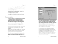
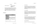
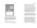
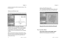
CybMod - User
Manual
A fuzzy modelling program for
process control
Table of Contents
Introduction . . . . . . . . . . . . . . . . . . . . . . . . . . . 1
System Requirements
............................... 2
Installing CybMod . . . . . . . . . . . . . . . . . . . . 2
How CybMod works . . . . . . . . . . . . . . . . . . . . 3
Why fuzzy ? . . . . . . . . . . . . . . . . . . . . . . . . 3
Fuzzy Sets . . . . . . . . . . . . . . . . . . . . . . . . . 6
Fuzzy relational models
. . . . . . . . . . . . . . . . . . . . . . . . . . . . . . 11
Relational model identification . . . . . . . . . 14
Dynamic Modelling . . . . . . . . . . . . . . . . . . 15
Tutorial . . . . . . . . . . . . . . . . . . . . . . . . . . . . .
Loading the data . . . . . . . . . . . . . . . . . . . .
Examining the data . . . . . . . . . . . . . . . . . .
Naming the fields . . . . . . . . . . . . . . . . . . .
Cross-correlation . . . . . . . . . . . . . . . . . . .
Building the model . . . . . . . . . . . . . . . . . .
Identifying the model
..............................
Testing the model . . . . . . . . . . . . . . . . . . .
Refining the model . . . . . . . . . . . . . . . . . .
What next ? . . . . . . . . . . . . . . . . . . . . . . .
18
19
20
21
22
24
Program Reference . . . . . . . . . . . . . . . . . . .
General program behaviour . . . . . . . . . . .
File Menu . . . . . . . . . . . . . . . . . . . . . . . . .
New System . . . . . . . . . . . . . . . . . . . .
37
37
38
39
27
29
31
35
Load a Model . . . . . . . . . . . . . . . . . . .
Save a Model . . . . . . . . . . . . . . . . . . .
Save a Model As . . . . . . . . . . . . . . . . .
Load Data . . . . . . . . . . . . . . . . . . . . . .
Save Data As . . . . . . . . . . . . . . . . . . .
Exit . . . . . . . . . . . . . . . . . . . . . . . . . . .
Data menu . . . . . . . . . . . . . . . . . . . . . . . . .
Data file Summary
...........................
Edit Field Names . . . . . . . . . . . . . . . . .
Outliers Removal . . . . . . . . . . . . . . . . .
Filter Data . . . . . . . . . . . . . . . . . . . . . .
Cross-Correlate Data
...........................
The Model Menu . . . . . . . . . . . . . . . . . . . .
Model Summary . . . . . . . . . . . . . . . . .
Manual Edit . . . . . . . . . . . . . . . . . . . . .
Identify a sub-model
...........................
Test a sub-model . . . . . . . . . . . . . . . .
Save test results . . . . . . . . . . . . . . . . .
Prediction Plot . . . . . . . . . . . . . . . . . . .
Residuals Plot . . . . . . . . . . . . . . . . . . .
The Analysis Menu . . . . . . . . . . . . . . . . . .
Do a Quick prediction
...........................
Model Completeness
...........................
Surface plots/Stacked plot . . . . . . . . .
Surface Plot/3D-Surface Plot . . . . . . .
The Controller Menu
..............................
The Logfiles Menu . . . . . . . . . . . . . . . . . .
The Help Menu . . . . . . . . . . . . . . . . . . . . .
The Main Window Dialogue . . . . . . . . . . .
39
39
39
40
40
41
41
41
43
43
45
47
50
51
52
54
57
59
59
59
62
62
63
66
67
67
68
69
70
Other Services from Process Cybernetics
.................................
Other products . . . . . . . . . . . . . . . . . . . . .
CybOnLine - On-line fuzzy modelling .
CybFIMC - Model-based fuzzy control
...........................
Services from Process Cybernetics . . . . .
Training . . . . . . . . . . . . . . . . . . . . . . . .
Consultancy . . . . . . . . . . . . . . . . . . . .
Software services
...........................
Contacting us . . . . . . . . . . . . . . . . . . . . . .
74
75
75
76
77
77
77
78
79
0
Introduction
Welcome to CybMod Vs 3.0. CybMod is a
powerful package for producing non-linear
process models using state of the art fuzzy
relational techniques. Models generated by
CybMod can be easily loaded into CybOnLine
and CybFIMC to provide fuzzy modelling and
control functionality to your current Microsoft
Windows-based SCADA system.
The process of building a model starts with
input/output data gathered from the system to be
modelled. CybMod includes tools which let you
examine this data, filter it, and remove outliers.
CybMod also includes cross-correlation tools to
help you generate appropriate structures for your
models. Once you have chosen a model
structure, building the model simply involves
some pointing and clicking with the mouse.
CybMod includes a variety of tools that you can
then use to verify the quality of the identified
model.
1
CybMod - User Manual
Chapter 1
We have developed CybMod from leading edge
research in fuzzy modelling and control in the
process industries. Process engineers have
designed the package with the process industries
in mind. We are continually developing our
products, and would be delighted to receive your
feedback.
System Requirements
Pentium PC running Microsoft WIndows 95, 98,
or NT.
Installing CybMod
Insert the diskette number 1 into the floppy disc
drive. Choose the Run command from the Start
menu, and in the Run window type:
Chapter 2
1
How CybMod works
Although it isn’t necessary to know anything
about fuzzy modelling to use CybMod, some
knowledge will help you get the most out of the
package.
Why fuzzy ?
a:\setup.exe
and then press enter.
Follow the on-screen instructions to complete the
installation.
Imagine a unit in a process plant. The behaviour
of the process is complex and is difficult to model
using conventional mathematical approaches.
Although they might not easily create a
mathematical model, the operators who control
the process obviously have a good
understanding of it - they must already have
some sort of process model in their heads.
The model the operators will have of their
2
CybMod - User Manual
3
CybMod - User Manual
Chapter 2
process will not be one which can be formed
from differential equations, but will instead be
made up of a set of rules which describe how the
process will behave under different conditions
(e.g. If the inlet concentration is low then the
reactor temperature will fall quickly).
If the operator’s model was rule-based and if
they could express these rules, then, at first
glance, it would appear to be simple to convert
the rule-based model into a form which a
computer could process (all computer languages
include “ if <condition> then <action>” type
statements). However, this isn’t very easy to do
using conventional mathematics.
To understand why, imagine we had obtained
two rules which described how an operator
controlled a temperature in a process:
If T is HIGH then set the steam pressure LOW
if T is LOW then set the steam pressure HIGH
Putting these rules into a computer program is
easy, provided we can explain to the computer
what LOW and HIGH temperatures, and steam
pressures, mean.
We need to define what we mean by these terms
by creating sets of LOW and HIGH temperatures
and LOW and HIGH steam pressures. The
definition will be highly dependant on the
4
CybMod - User Manual
Chapter 2
application. A high temperature in a water bath
will be much different from a high temperature in
a catalytic convertor. Here, we might say that all
temperatures less than 50oC were LOW, and all
temperatures greater than 80oC were HIGH. For
the steam pressure we might say a LOW
pressure is 0.5 barg and a HIGH pressure is 5
barg.
What happens if we use the rules and set
definitions to control the process? When we start
the process, the temperature is below 50oC, and
so is classified by the computer as LOW. This
means that the computer applies a HIGH steam
pressure of 5 bar, and the process heats up. As
the process temperature crosses the 50oC
boundary, the computer has a problem - it has no
rule to tell it what to do. A temperature of 51oC
(or any other temperature between 50oC and
80oC) belongs to neither the HIGH nor the LOW
temperature sets.
If we had foreseen this problem, we might have
added code to tell the computer not to change
anything when the temperature doesn’t belong to
either temperature set. Then, as the temperature
crosses the 50oC boundary, the controller will
maintain the steam pressure at the high value,
and the temperature will continue to increase.
As the temperature crosses the 80oC boundary,
another unpleasant thing happens. At 79.9oC the
5
CybMod - User Manual
Chapter 2
computer will maintain a HIGH steam pressure,
but at 80oC the HIGH temperature rule will
activate, and steam pressure will suddenly switch
to its LOW value. The controller will then
maintain the LOW value until the temperature
drops to 50oC, and then the steam pressure will
suddenly switch to HIGH, resulting in a
temperature which oscillates between roughly
50oC and 80oC.
The problem with our system is that we haven’t
defined properly what a human means by the
terms HIGH and LOW, or BIG or SMALL, or any
of the other adjectives which are used in
everyday life. Humans don’t make crisp
boundaries to the sets they use to describe the
world. In our process example the operator
would probably regard 70oC as quite a HIGH
temperature, not as HIGH as 80oC, perhaps, but
still sufficient to require some attention. These
leads to the idea of Fuzzy Sets.
Fuzzy Sets
A fuzzy set is a set where the elements can
belong to the set with a variable degree of
membership. By convention, this degree, or
grade, of membership is a number which varies
between zero and one, with zero showing that
the element doesn’t belong to the set, one that it
belongs completely to the set, and intermediate
grades showing intermediate membership. In
6
CybMod - User Manual
Chapter 2
process control problems, where we are usually
dealing with continuous variables rather than
discrete elements, the grade of membership of a
variable to a fuzzy set is expressed as a
continuous membership function. These
membership functions can take many forms, but
the most common, and that used in CybMod is
the triangular membership function.
Figure 2.1 shows a group of four typical
triangular membership functions defined over a
variable’s range.
Three values can completely define each
membership function; the variable’s value at the
leftmost edge of the function where the grade-ofmembership (GM) is zero; the set centre where
the GM is one; and the rightmost edge of the set
where the GM is again zero. If we define a group
of reference sets to be fully overlapping, then the
rightmost edge of a set is at the same value as
the centre point of the immediately following set,
and as the leftmost edge of the set after that.
Just setting the centre points of each set in the
series can completely define a group of
overlapping triangular reference sets. All set
definitions in CybMod are fully overlapping
triangular sets, because of the simplicity of
definition, and because they possess very useful
computational properties.
7
CybMod - User Manual
Chapter 2
The two end sets of the group in fig 2.1 illustrate
other features of triangular fuzzy sets. The left
most set has a left value equal to its centre
value, and is called a closed end set. Variable
values outside a closed end set (to the left in this
case) have zero membership in any of the sets.
This can be useful in situations where an error
needs to be flagged if a variable value falls
outside a certain range. Usually, however, an
open end set, such as the rightmost of the group,
is much more useful. An open set has a
boundary which extends to infinity which means
Chapter 2
end sets in CybMod are open sets.
A group of fuzzy sets defined over a variable’s
range are usually called the reference sets for
the variable, because they establish a frame of
reference for the computer to understand rules
about the system. We can give reference sets
linguistic labels ((Z)ero, (S)mall, (M)edium and
(L)arge in figure 2.1). This is useful when working
with rule-based models, but is unnecessary and
cumbersome when working with the relational
models described later in the chapter.
Going back to the example described earlier in
the chapter, we could define a set of reference
sets for the process temperature as shown in
figure 2.2.
Figure 2.1 - Triangular reference sets
Using these fuzzy reference sets for the process
temperature now produces a controller with a
much more sensible control action. At
temperatures below 50oC the temperature
completely belongs to the LOW set and belongs
to the HIGH set with a zero GM. This means that
the rule associated with low temperature will fire
at full strength, and the steam pressure will be
set to its LOW value. As the temperature moves
above 50oC, the GM in the LOW set starts to fall
below one and the GM in the HIGH set starts to
increase above zero. This causes the rule
that all variable values on the open side of the
set centre belong to the set with a GM of one. All
8
CybMod - User Manual
9
CybMod - User Manual
Chapter 2
Chapter 2
this makes them a very powerful general
purpose tool for process modelling and control
applications.
Fuzzy relational models
associated with LOW temperatures to fire less
strongly, and that associated with HIGH
temperature to fire more strongly. After
defuzzification this results in a steam pressure
which gradually increases from a LOW value up
to a HIGH value in the region of temperatures
between 50oC and 80oC.
The idea of obtaining qualitative process models
from knowledgeable operators is attractive in
theory, but difficult to do in practice. Operators
often find it difficult to express all the knowledge
they have in a coherent set of rules. When
different operators are interviewed, they often
come up with different, sometimes conflicting,
sets of rules about the process behaviour and
the best way to control it. As a result,
applications of fuzzy control based around rulebased systems all have to go through a period of
difficult and expensive knowledge engineering
where expert interviewers obtain rule sets from
operators and then, after several iterations, refine
them to a complete and consistent set of rules.
That is really all that there is to fuzzy modelling.
In this simple example the same controller could
be produced more easily with a simple linear
function, but in practical systems more inputs are
used, and more reference sets are used for each
variable, leading to non-linear relationships
between the inputs to the model and the output.
Fuzzy models can represent any non-linear
function, to any required degree of accuracy, and
Another disadvantage with the rule-based
approach for control system design is that the
rules the operators give are often very
conservative. A human operator is unable to
devote all their attention consistently to a single
control problem throughout an entire shift. This
means that they make control actions which don’t
move the process particularly quickly, and so
give them time to focus their attention elsewhere.
10
11
Figure 2.2 - Reference sets for the temperature
controller
CybMod - User Manual
CybMod - User Manual
Chapter 2
An alternative to the rule based modelling
approach is fuzzy relational modelling. The idea
behind a relational model is that relationships
exist, to some extent, among all the AND
combinations of the inputs (e.g. HIGH flow AND
MED concentration), and the output fuzzy
reference sets. These relationships are fuzzy
relationships, and are held in a relational array
as values between zero and one (zero
representing no relationship and one a very
strong relationship).
The modelling problem now becomes the
assignment of appropriate values to the entries in
the relational array. Translating rules obtained
from knowledge engineering into a relational
array format is possible, but it is much more
common, and useful, to obtain the relational
array directly from measured process
input/output (i/o) data through an identification
algorithm.
Obtaining the model directly from process i/o
data has two important advantages over the rulebased knowledge engineering approach.
a) Process i/o data is easily available in most
process plants. Although obtaining a good,
representative, set of i/o data can be difficult
sometimes, it is still much less time
consuming than generating a complete and
consistent rule-base.
12
CybMod - User Manual
Chapter 2
b) The model which is obtained will be a
representation of the process i/o relationships
present in the identification supplied. It will
not represent the operator’s opinion of, and
prejudices about, the process behaviour.
Including such a model in a model-based
control scheme will allow much tighter control
than that which could be achieved from the
knowledge engineering approach.
Although a relational model doesn’t usually
incorporate human operators knowledge directly,
it does use the same qualitative structure that
humans use to deal with real world complexity.
This provides computer based systems with a
very powerful way of dealing with complex
process behaviour.
Relational model identification
There are a wide range of different ways of
identifying fuzzy relational models. The method
used in CybMod, direct-least squares, is one of
the best and is described below. It isn’t
necessary to know how this identification
algorithm works to use CybMod, and the details
are included for information only.
A fuzzy relational model is usually represented
13
CybMod - User Manual
Chapter 2
by
Y'R  X1  X2 ÿ Xn
where Y
Xi
R
"
=
=
=
=
Possibility vector of the output
Possibility vector of the ith input
Fuzzy relational array
Fuzzy compositional operator
A Possibility Vector is a vector made up of the
grades of membership of a particular variable
value in each of the reference sets used to
describe that variable. The fuzzy compositional
operator is the method used to combine the
inputs and relationships to form a prediction;
there are several different ways of doing this.
If a particular form of fuzzy composition is used
(summated-product), and a property of fully
overlapping reference sets invoked, then the
relational model equation can be expressed as
Chapter 2
This form of the relational equation is linear in
the parameters (R’), and can be identified using
normal linear least-squares techniques. CybMod
uses a recursive least-squares identification
algorithm which allows multiple i/o data sets to
be easily processed.
Dynamic Modelling
Most models used directly for control are
dynamic, that is they model not only how big
changes are, but also how quickly they take
place. A fuzzy relational model is not inherently
dynamic, but is simply a static mapping between
combinations of inputs and the corresponding
output. However a relational model can be
formed to represent a discrete-time(sampled)
dynamic system.
Consider the following first-order dynamic
process
dy
'f ( y, u1, ÿ ,u n)
dt
y'R ). kron (X1 , X2 , ÿ , Xn)
where y
=
R’ =
kron() =
14
Scalar (non-fuzzy) value of the
output
Reordered fuzzy relational array
Kronecker tensor product (just an
ordered multiplication) of the input
possibility vectors
CybMod - User Manual
where y =
ui =
f =
process output
ith process input
some function
a backward difference discrete time
15
CybMod - User Manual
Chapter 2
approximation of this process can be formed as:
y(k)&y(k&1)
'f ( y(k&1) , u1(k&1),ÿ, u n(k&1))
∆t
where k =
∆t =
current sample number
sampling interval
Chapter 2
process deadtime. This deadtime will either be
real and/or will be included to approximate
higher-order process dynamics ( as a first-order
+ dead-time model).
A typical fuzzy relational dynamic model for a
process will therefore look like this:
Y(k)'R  Y (k&1)  U1 (k&1&τ1)  ÿ  Un (k&1&τn)
and, after rearrangement
y (k)'f ) (y(k&1) , u1(k&1), ÿ , u n(k&1))
where f’ is a modified form of the function f.
where Y
Ui
k
τi
=
=
=
=
possibility vector of the output
possibility vector of process input i
current sample
dead-time on input i
This can easily be expressed as a fuzzy
relational model:
Y(k)'R  Y(k&1)  U1(k&1)  ÿ  Un(k&1)
Higher-order dynamic models can be created
simply by adding additional lagged outputs (and,
perhaps, inputs) on the right-hand side of the
relational equation. In practical situations it
usually isn’t a good idea to go beyond first-order
model dynamics because of the problems in
obtaining complete and representative data.
In most practical situations additional lags will be
introduced into the input variables to represent
16
CybMod - User Manual
17
CybMod - User Manual
Chapter 3
Chapter 3
Loading the data
Start CybMod by selecting CybMOd from the
Windows start menu.
2
From CybMod's File menu, select the Load Data
item. This will bring up a standard Windows file
dialogue. Select the file 'boxjen.dat' from the
c:\CybMod directory. CybMod's Window display
will change to show the model building dialogue.
Tutorial
The best way to learn how to do something is to
do it. This chapter introduces you to the use of
the CybMod program by going through the
stages involved in building a model of a simple
dynamic process. You should read the manual
alongside your computer and follow the exercise
through.
A set of sample data (boxjen.dat) is included with
CybMod, and can be found in the c:\CybMod
directory. This data is the famous Box-Jenkins
laboratory furnace data and consists of three
fields of data: the sample number; the fuel
flowrate deviation; and the off-gas concentration.
The object is to build a dynamic model of the offgas concentration.
18
CybMod - User Manual
19
CybMod - User Manual
Chapter 3
Chapter 3
giving you a chance to look at how the data is
distributed.
Examining the data
Before we start to build a model we need to look
at the data that we have just loaded. From the
Data menu, select the Data file summary item.
A window will appear which gives a summary of
the information contained in the data file.
Have a look at the data fields. Field_0 is just the
sample number, and will produce a rather
strange looking histogram! Field_1 is the fuel
flowrate deviation, and the histogram shows an
approximately Gaussian distribution. Field_2 is
the off-gas concentration, and the histogram
shows a distribution which is slightly skewed
towards higher gas concentrations.
Naming the fields
It's easy to get confused when referring to the
fields of data as 'Field_0', 'Field_1', etc, and so
it's worthwhile giving them meaningful names
early in the model building process.
From the Data menu, select the Edit Field
Names item.
From the summary we can see that the data file
consists of 296 samples of data, each containing
three data fields. Information about the individual
data fields can be obtained by selecting the field
name from the Field Information list box. The
Histogram button plots a histogram of the data,
The
list box in
this dialogue gives you access to all the field
20
21
CybMod - User Manual
CybMod - User Manual
Chapter 3
Chapter 3
names stored internally by CybMod. To change a
name simply select a field from the list box and
then edit it using the keyboard. To edit another,
just repeat the process.
Change 'Field_0' to 'Sample No', 'Field_1' to
'Fuel', and 'Field_2' to 'Conc'.
Press OK to tell CybMod to save the changes.
Cross-correlation
Cross-correlation is a statistical technique which
is sometimes useful in detecting dynamic
relationships between variables. It works by
calculating the correlation coefficient between
two variables at a range of different lags.
To run a cross-correlation analysis, select
Cross-Correlate Data from the Data menu.
Two list boxes are displayed on the dialogue box
which appears: 'Input variable'; and 'Output
variable'.
Select 'Fuel' as the input variable, and 'Conc' as
the output variable, and then press the XCorr
button to carry out the cross-correlation.
After a few seconds a graph will appear on the
right of the dialogue. This graph shows the
results of the cross-correlation analysis. The x22
CybMod - User Manual
axis is the relative lag between the input and the
output. The y-axis is the correlation coefficient.
High absolute values of the correlation coefficient
at positive lags indicate a causal relationship
between the input and the output, and high
values at negative lags indicate a causal
relationship between the output and the input
(due to feedback in the process).
In this example, a high negative correlation
occurs at a lag of five samples ( to zoom in on
the graph, left-click and drag select the area you
want magnify, and right-click to restore the
graph). This gives us an idea of the lag that we
might want to apply to the input in the dynamic
model we shall be building.
23
CybMod - User Manual
Chapter 3
Chapter 3
Cross-correlation suffers from a number of
limitations. In cases where an output is affected
by several inputs, and these inputs change in a
non-random manner, the cross-correlation
results can be impossible to interpret. Also, with
high-order processes, the best lag on the input
can be over-estimated.
Building the model
If you haven't already done so, close the crosscorrelation dialogue. On the main Window you'll
see a list box which lets you select the output for
your new model. From this list box select 'Conc'.
Below this is another list box which allows you to
select the default number of reference sets to be
applied to each input in the new model. For now
just leave this at '2'.
For this example, however, we want to build a
dynamic model, so leave the lagged output as it
is.
The current model structure is shown as a fuzzy
relational equation. By default, a lagged value of
the output is used as a model input creating the
basis of a first-order dynamic model. If you want
to create a steady-state model, just double-click
the lagged output and change it to the input you
want (remember to set the lag to zero).
At the bottom of the display the centre points of
the reference sets for the model variables are
listed. These sets are automatically created by
spacing them equally between the minimum and
maximum values present in the data set for the
variable in question. Usually, you should at least
change the end set positions to the minimum and
maximum values you would ever expect to see in
the 'real world'. To change the set positions
double-click on the reference set centre points.
This brings up a set editing dialogue. To change
the position of a particular centre point, double-
24
25
To create the model press the Create button. A
new card will be created containing your initial
model structure.
CybMod - User Manual
CybMod - User Manual
Chapter 3
click on the value in the reference set centres
Chapter 3
at '2', and press the OK button.
A new input (Fuel(k-5)) will be added to the
model structure display. Change the values of
the reference set centres for this variable to '-3'
and '3'.
Identifying the model
Now that we have set the model structure we
need to identify the relational array entries. To do
this select the Identify a sub-model item from
the Model menu. Make sure that the 'Model 1'
tab is selected on the main window display (all
the modelling menus refer to the currently
selected sub-model).
frame, and then edit the value in the edit box that
pops up. For this example, change the two set
centres to 40 and 65.
Click the Done button to close the 'Edit reference
sets' dialogue.
We are now ready to add another input to the
model. Click the Add a new Input button on the
main window dialogue. Select 'Fuel' from the list
box in the dialogue that appears. Set the lag
value to '5' (the value obtained from crosscorrelation), leave the number of reference sets
26
CybMod - User Manual
CybMod provides two ways of presenting the
data to the identification algorithm. The first is
sequentially where the data is presented in
sequence from the first sample to be used to the
last. The second is randomly, where a fraction of
the total number of examples are chosen at
random from the data (the same example can be
chosen several time, so that 75% on the dialogue
doesn't mean that three-quarters of the data will
be used).
27
CybMod - User Manual
Chapter 3
If you intend to use all the data for identification,
or you want to identify only on a fixed portion of
the data, then sequential presentation is best. If
you intend to use only part of the data for
identification, but the whole set for testing, then
random presentation is best since samples will
be chosen across the whole range of data. This
is useful if the data covers several different
Chapter 3
example, choose random presentation by
selecting the Use data drawn randomly option.
The % of data to be used is the number of
presentations of data to the identification
algorithm expressed as a percentage of the total
number of samples in the data (e.g. if a file
consists of 500 samples, a value of 150% will
present 750 examples to the identification
algorithm). The random number seed is used to
initialise the random number generator. Leave
both as they are, and press the OK button to
start the identification process. A progress bar
will appear, and, after a few seconds, the
dialogue will disappear - identification is now
complete.
Testing the model
To test the model, select the Test a sub-model
item from the Model menu.
The dialogue allows you to set the range of
samples to be included in the test. The Steps
ahead list allows you to specify how far ahead
you want the model to predict. SIngle-step ahead
ing
es.
For
28
operat
regim
this
CybMod - User Manual
29
CybMod - User Manual
Chapter 3
Chapter 3
Refining the model
Model building is an iterative process where
different models are built, compared against each
other and refined. CybMod includes several tools
to help you with this process.
prediction,
where the
current
value of the real
output is
used, isn't
too much
of a
challenge.
Multi-step
ahead prediction, where predictions are based on
one or more previous predictions is a much better
way of assessing model quality. The most difficult
test is the 'free running' predictor where the model
is only supplied with the initial value of the output,
and all subsequent predictions are based on
previous model outputs.
Select 'Free' from the list to run the model as a
free running predictor. Press the Test button.
After a few seconds summary results of the test
will appear at the bottom of the dialogue. Note
that the mean squared error is 2.04, the maximum
error is 4.57, and the AIC (Akaike Information
Criterion, a measure of accuracy vs. complexity)
is 0.742. Press the Cancel button to close the
test dialogue.
30
CybMod - User Manual
One useful thing to do is to look at the model
residuals (the differences between the predicted
and actual outputs). CybMod lets you plot the
residuals against all the data fields
(Model|Residuals plot), and also lets you crosscorrelate the residuals (Model|XCorr Residuals)
against the data fields.
For now, cross-correlate the residuals against the
'Fuel' ( the dialogue works just like data crosscorrelation, except that only the input needs to be
set). Your results should look like this :
Notic
that
31
e
we
CybMod - User Manual
Chapter 3
are getting a strong correlation of the residuals
with the 'Fuel' at a lag of 4 samples. This lag was
not used in the original model, and could be worth
evaluating more carefully.
Close the cross-correlation dialogue by pressing
the Done button. On the main window dialogue
for model 1, double-click on the 'Fuel(k-5)' term in
the model structure display. This will bring up an
edit dialogue.
Chapter 3
in model performance (also reflected in the AIC
dropping to -0.027).
The maximum error, however, hasn't been
reduced by much; it still has a value of 3.83. Have
a look at the prediction plot (Model|Prediction
plot). You should see that the model tracks the
real process output closely for most of the range,
but loses accuracy in the last thirty or so samples
- it looks as though the process has changed in
some way in this region, and more experimental
investigation would be needed to find out what
was happening.
The model we are using at the moment has only
two reference sets defined for each variable, and
as a result is almost linear. Highly non-linear
processes need more reference sets defined on
one or more of the inputs (depending where the
non-linearity is). Look at the residuals plot for the
fuel input
Change the lag on the 'Fuel' variable from 5 to 4,
and press the OK button to complete the edit.
Identify the model again using random
presentation and the default identification
parameters.
Run a model test with a free running predictor.
You should find that the mean squared error has
dropped to 0.948 indicating a significant increase
32
CybMod - User Manual
33
CybMod - User Manual
Chapter 3
The largest values of the residuals seem to be
clustered close to the '0' value, which could
indicate the presence of a non-linearity in this
region. We need to add some more reference
sets to the 'Fuel' variable in this region to check
this.
Close the residuals plot and double-click the
'Fuel(k-4)' field in the model structure on the main
window dialogue. In the variable edit dialogue
which appears, change the number of reference
sets to '4'. Press the OK button to make the edit
and note that the reference sets defined on this
variable have increased in number.
Double-click the reference set definitions for the
'Fuel' variable in the Reference Sets frame to
bring up the set centre editing dialogue. Change
the values of the sets centres to (-3, -0.1, 0.1, 3.0)
and exit the editing dialogue.
Now identify the model again (still using random
presentation and default parameters). Test the
model as a free running predictor. The value of
the mean squared error should have dropped to
0.874.
Although it looks as though we now have a better
model, we have to be careful. The number of
entries in the relational array have increased from
four (2 x 2) to eight (2 x 4), and so that it is not
surprising that the model error has reduced. The
34
CybMod - User Manual
Chapter 3
AIC which balances model performance against
model complexity has also reduced indicating that
the change we have made could be worthwhile. If
you look at the residuals plot for the fuel,
however, you'll find that the largest are still
clustered near zero, and so we haven't solved
that problem.
The largest residuals actually come from the end
of the data set, where, from earlier, we think that
the process has changed in some way. The fuel
flowrate in this region coincidently has values
close to zero, and it is this and not non-linearity
which is producing the cluster of residuals near
zero 'fuel' values.
It is probably best in this case to use only two
reference sets on each variable. This coincides
with other investigations which have been carried
out on this data set, and which have concluded
that the process is nearly linear in the range
which the data covers.
What next ?
Process modelling is an art. Although CybMod
provides a useful range of tools, it will take
experience to know when it is best to use them,
and how best to interpret the information which
comes from them.
35
CybMod - User Manual
Chapter 3
A good understanding of the process to modelled
is very important for effective modelling. Use your
own process data and practise building models.
Are the models sensible? Are the lags
reasonable? Does the prediction surface slope in
the right direction? The more you use CybMod,
the better you'll get !
Chapter 4
3
Program Reference
This chapter describes the functions available in
CybMod in detail. We recommend that you get
familiar with the program using the tutorial first,
and then use this chapter to fill in you knowledge.
General program behaviour
The information you will see in CybMod displays
is colour coded according to what you can do with
it:
Yellow background - information only
Blue background -
36
CybMod - User Manual
37
can be double clicked to
bring up additional
CybMod - User Manual
Chapter 4
Chapter 4
dialogues
White background
-
data can be typed in
directly from the
keyboard
Most of the 2-D graphic displays can be zoomed
to look at data in finer detail. To zoom in, left-click
and drag-select the area of interest and then
release the mouse button. Click the right mouse
button to reset the display back to the original
size.
New System
Selecting this menu item will clear CybMod of all
currently loaded model and data, and reset the
program for a new problem. If you haven’t saved
your model, or modified data, you’ll be given the
option to do so.
Load a Model
Loads a previously saved model. If the number of
data fields used to develop the loading model is
different from the number of fields in any currently
loaded data, then loading will be stopped and an
error announced.
File Menu
Save a Model
Saves the currently loaded model - all submodels
will be saved, along with tagname definitions,
model summary information, and the model log.
The model is saved with the default extension
‘*.pcg’, and the log file with the extension ‘*.mlg’.
Save a Model As
Allows you to save previously loaded model
38
CybMod - User Manual
39
CybMod - User Manual
Chapter 4
under a different name.
Chapter 4
CybMod either by filtering it, or by removing
outliers.
Load Data
Exit
Loads a process i/o data file. Doing this when
CybMod is empty will cause the main window to
change to the model creation dialogue. If a
model, or another datafile, is currently loaded
then CybMod will check that the field count is
consistent with the new data, if it isn’t then
loading will be aborted and an error will be
flagged. Loading new data will erase the previous
data set.
Data files for CybMod have to be standard ASCII
text. The data is arranged with the fields in
comma, space, or tab delimited columns, and the
records (samples) in rows. Non-numeric
information in a data file will cause an error on
loading.
Exits the program, prompting you to save any
modified models and/or data.
Data menu
The data menu provides you with some tools to
exam, modify, and process i/o data files.
Save Data As
Data file Summary
Allows you to save the datafile under a different
name, and also saves the data log. The data is
saved with the default extension ‘*.dat’, and the
log file with the extension ‘*.dlg’.
This is only useful if you modify the data within
40
CybMod - User Manual
Shows a dialogue containing summary
information about the currently loaded data. The
dialogue lists the model file name, the number of
samples of data, and the number of fields in each
sample.
41
CybMod - User Manual
Chapter 4
Chapter 4
Edit Field Names
The lower part of the dialogue, enclosed in the
frame, allows more detailed information to be
obtained about each field within the data. If you
select a data field in the list box, then CybMod will
calculate the maximum, minimum and mean
values of the data, and its standard deviation.
Clicking the ‘Histogram’ button will generate a
histogram showing the distribution of the values
of the data in the currently selected field.
When
a new
data
file is
loaded the fields are automatically named
‘Field_0', ‘Field_1', etc. It is much less confusing if
the data fields are given meaningful names, and
this dialogue allows you to do this. Simply select
the field you would like to rename from the list of
available fields, and type the new name in the edit
box. Continue to select and edit as many names
as you require, and press ‘OK’ to finish. The
‘Cancel’ button will close the dialogue without
saving the edited field names.
Outliers Removal
Sometimes process data will contain values
which are unreasonably large or small. The most
common reason for these outliers are ‘spikes’
from analytical instruments, with gas analysers
42
CybMod - User Manual
43
CybMod - User Manual
Chapter 4
being particularly prone to this problem. These
Chapter 4
acceptable data values to anything you wish by
editing the boxes in the frame in the lefthand side
of the dialogue. Pressing the ‘Try it’ button plots
the new limits on the graph, highlights the outliers
with red crosses, and provides a count of the
outliers at the bottom of the dialogue. At this
stage the data is unchanged.
Pressing the ‘Apply It’ button will apply CybMod’s
outlier removal. CybMod does this by simply
replacing outliers with a value interpolated from
the nearest valid data. Once this is done, the data
set loaded in CybMod has been changed
irrevocably - if you want to return to the old data,
then you must reload it.
values need to be removed prior to model
identification to prevent them from skewing the
results.
The outliers removal dialogue provides access to
CybMod’s routine for removing outliers. Select the
field to be processed from the ‘Datafield’ list. A
plot of the data will appear on the graph on the
right-hand side of the dialogue. Two dotted green
lines also appear on the plot showing the
maximum and minimum acceptable values of the
data. This is initially set to 5% outside of the
maximum and minimum values in the data set.
You can change the maximum and minimum
44
CybMod - User Manual
Outlier removal should be used with caution. It is
necessary to remove genuinely spurious data, but
removal of data because it ‘doesn’t look right’ can
lead to seriously flawed models. Most data will
not require outlier removal.
Filter Data
Process i/o data gathered for model identification
should ideally already be properly filtered using
analogue and digital filters. In some cases,
however, particularly in initial modelling
investigations, only unfiltered or poorly filtered
data is available. CybMod includes a simple firstorder filtering algorithm to deal with this.
45
CybMod - User Manual
Chapter 4
Chapter 4
The ‘Do it’ button actually applies the filter to the
data field. The only way to restore the original
data will be to reload it into CybMod.
The ‘Done’ button simply closes the dialogue.
Filtering is something that has to be done with
caution. Applying a filter can remove noise, but it
removes some useful data too. Also you need to
remember that if you have applied a filter to build
a model in CybMod you must make sure that the
same filter is applied to SCADA data prior to it
being passed to CybOnLine or CybFIMC loaded
with that model.
The filter parameters are specified through the
filter dialogue. The data field to be filtered is first
selected from the list box. This will trigger the
production of a graph of the data in the right-hand
side of the dialogue.
The two edit boxes on the left of the dialogue
allows the sample time at which the data was
gathered to be set, and a filter time constant to be
specified.
The ‘Try it’ button lets you try the filter on the data
without actually changing the data stored in
CybMod. The graph will show the effect of the
filter parameters you have chosen. Increasing the
value of the filter time constant will increase the
amount of filtering which takes place.
46
CybMod - User Manual
Cross-Correlate Data
Cross-correlation is a tool to help in spotting
relationships in dynamic data. It essentially
involves calculating the correlation coefficient
between an input and an output data series with
different values of lag between the data.
Cross-correlation can be carried out in CybMod
through the Cross-Correlation dialogue. The input
and output data are selected from the list boxes
(it is possible to select the same data for each
and carry out an auto-correlation).
The maximum lag over which the correlation will
be evaluated can be adjusted by changing the
number in the ‘maximum lag’ box.
47
CybMod - User Manual
Chapter 4
Sometimes false correlations can be detected
when both the input and output are subjected to
Chapter 4
The x-axis of the graph shows the relative lag of
the input to the output. Positive values of lag
represent causal relationships between the input
and the output. Negative values represent causal
relationships between the output and the input
(feedback relationships).
The y-axis of the graph shows the value of the
correlation coefficient. Positive values indicate a
positive gain between the input and output, and
negative values a negative gain.
Two yellow and two green dotted lines run
horizontally across the graph. These are the 95%
(yellow) and 99% (green) confidence limits on the
correlation coefficient based on a t-test.
an external influence which cause both to move.
To prevent this from happening a de-trending
filter is applied to both sets of data. The order of
this filter can be adjusted by editing the ‘Filter
Order’ box. The filter order shouldn’t be changed
unless you have a good reason for doing it.
Pressing the ‘XCorr’ button will carry out the
cross-correlation calculation. This will take a few
seconds, and the time required will increase with
the size of the data set, the maximum lag, and the
filter order. When the calculation is complete the
results will be displayed in the graph on right of
the dialogue.
48
CybMod - User Manual
The solid line on the graph represents the results
of the cross-correlation. The strongest peak
(positive or negative) on the positive side of the xaxis can give a reasonable first estimate for the
‘dead-time’ between the input and the output.
Cross-correlation works best for processes which
are dominated by one big capacity (a single big
time constant). In these cases a clear peak will be
observed and this can be used with some
confidence to form a model structure. When
process involved multiple capacities with similar
time constants, then the results are less useful.
The best that can be hoped for in these cases is a
rough idea of the most appropriate lag that can be
49
CybMod - User Manual
Chapter 4
refined by trial and error during model building.
Cross-correlation results can also be difficult to
interpret when an output is subject to several nonrandom inputs.
The Model Menu
The
model
menu
is only
activat
ed when a
submodel is
selected from the main window model building
dialogue. Most of the functions on the model
menu (apart from the Model Summary) act only
on the currently selected sub-model.
50
CybMod - User Manual
Chapter 4
Model Summary
The model summary simply provides information
about the model you are working on. The
summary applies to, and is the same for, all the
sub-models.
You can enter a suitable system name - the
system name is used by CybOnLine as the topic
name for DDE conversations with the SCADA
package. If you intend to run multiple on-line
modellers, then you need to make sure that the
models they use are allocated different system
names.
51
CybMod - User Manual
Chapter 4
The ‘General Remarks’ is just text that is saved
along with the model. You can use it to add
reminders to yourself about the model.
Manual Edit
Chapter 4
The manual editing dialogue works by taking twodimensional slices through the relational array.
The variables to be used for the x and y axes are
selected from the two list boxes, and the ‘slice’
appears in the big box on the righthand side of
the dialogue. The values highlighted with a yellow
background along the top of the box are the
centre points of the reference sets for the ‘xvariable’. The yellow highlighted values down the
lefthand edge are the reference set centres for
the ‘y-variable’. The values in the edit boxes in
the centre of the box are the relational array
entries, and can be changed simply by typing in a
new value.
In cases where the model has more than two
inputs, there will be more than one possible 2-D
slice. To access the individual slices a list box
appears at the bottom of the display when three
or more inputs are present. Clicking on an input in
this list brings up a popup menu showing the set
centres for that variable. Clicking on one of these
brings up the appropriate 2-D slice.
Manual editing allows you to go right into the
relational array and change the values stored
there. Since changing relational array entries is
likely to have wide ranging effects, it is something
that should only be attempted with extreme care.
It is, however, sometimes useful in situations
where data is missing or suspect.
52
CybMod - User Manual
Once again manual editing in not something to
undertake lightly. There are usually better ways of
dealing with model or data problems.
53
CybMod - User Manual
Chapter 4
Chapter 4
set for identification (perhaps to keep the rest for
testing). The maximum number of samples
available for identification will be less than the
number of samples in the data if lags are present
in the model structure.
Identify a sub-model
The identification parameters allows you to
control the identification algorithm. If the ‘Clear
Model First’ box is checked then the existing
model will be erased prior to the identification. If
you are identifying a model from multiple data
sets then you would need to make sure that this
box is unchecked on processing the second and
subsequent data sets. The ‘Forgetting Factor’
value allows the forgetting factor on the recursive
least-squares algorithm to be adjusted. If this is
moved to a value less than one then more recent
information will be given more weight in the
identification process. This is only useful if you
believe that the process is non-stationary. Unless
you have a very good reason to change it then
leave it at one !
There are two versions of this dialogue. The first,
shown above, is used when the ‘Use data
sequentially’ option is selected. In this case
identification is carried out by moving through the
data from the start sample sequentially to the end
sample.
The start sample and the end sample can be
adjusted if you wish to use only part of the data
54
CybMod - User Manual
Pressing ‘OK’ will start the identification process.
This can take quite a long time with big data sets,
lots of model inputs and lots of reference sets - if
you are finding it too long, then the process can
be stopped by pressing the ‘Cancel’ button.
The other form of the identification dialogue
appears when the ‘Use data drawn randomly’
option is selected.
55
CybMod - User Manual
Chapter 4
Chapter 4
The dialogue allows the percentage of data to be
used for identification and the random number
seed to be specified. Choosing the same random
number seed will always result in the same
sequence of data being drawn from the data set.
Test a sub-model
W
hen this
op
tion is
chosen identification will be carried out with a
portion of the data drawn at random from the
whole set of data. This is useful where only part
of the data is to be used for identification, but
where the data is non-uniform with one operating
state at the start of the data and another at the
end. Building a model sequentially would result in
a very good model of the data at the start, and no
model at all of the end condition.
56
CybMod - User Manual
This
dialogue
allows a prediction test to be run on a sub-model
using the currently loaded data set. The range of
data to be used for the test can be set by editing
the start and end sample values.
57
CybMod - User Manual
Chapter 4
The ‘Steps ahead’ list controls the way the
prediction is carried out. Remember that a
dynamic fuzzy model is generally of the form
y(k)'f (y(k&1) % some inputs)
if the current value of y (y(k)) is predicted using
the value of y(k-1) from the i/o data (single-step
prediction), then good prediction results are really
easy to acheive. In fact a pretty good single-step
predictor is just
y(k)'y(k&1)
Although this gives good single-step prediction
results, it is pretty useless for control and on-line
modelling purposes. This means that single-step
prediction performance is not a particularly good
measure of a model.
Multi-step prediction, where the model has to
predict several steps ahead, using its previous
predictions as a base for the next, is a much
better test. The most stringent test is a freerunning prediction where the model is only told
the first value of the output, and has to generate
the rest of its predictions based on its own
previous outputs.
The ‘Test’ button starts a test and the ‘Cancel’
button closes the dialogue. When a test is
complete a frame will appear at the bottom of the
58
CybMod - User Manual
Chapter 4
dialogue giving summary test statistics.
Save test results
Selecting this menu item after a model test will
bring up a dialogue allowing you to specify a
filename and location for saving the test results.
The results are saved with the original data
occupying the first fields, and the model
prediction placed in the last field. Where lags are
present in model, the first predictions can't be
made and are instead replaced with the actual
value of the output.
Prediction Plot
This produces a graph comparing the predicted
and actual outputs from the process. The menu
item isn’t available until a test has been run on
the current sub-model.
Residuals Plot
Generates a plot of the model residuals (the
difference between the predicted and actual
outputs), against either the sample number or
each of the data fields.
Simply select the variable you want to plot the
59
CybMod - User Manual
Chapter 4
Chapter 4
XCorr Residuals
residuals against from the list.
By examining the residuals plot you can get an
indication that your model is missing some
important variables. The residuals should be
evenly distributed on either side of the x-axis - if
they are not you may have a problem.
The residuals plot has to be used with caution in
dynamic systems since there may be a lag in the
effect of variables on the output. It is useful,
however, for giving a quick check on the
suitability of a sub-model.
60
CybMod - User Manual
This dialogue allows you to cross-correlate the
model residuals against each of the fields of data.
A high value of the correlation coefficient
indicates a significant contribution to the model
error. If it occurs for fields or lags that are not
currently included in the sub-model, then it
probably means that the model’s prediction
performance could be improved by including the
data field as an input. Remember that a high
correlation does not necessarily imply that adding
that variable will reduce the prediction error by a
worthwhile amount.
61
CybMod - User Manual
Chapter 4
Chapter 4
can be used to obtain predicted output values for
any desired set of inputs. It’s useful for checking
particular points on the sub-models prediction
surface.
The Analysis Menu
Th
e analysis
me
nu provides
you
with some
tool
s to analyse
the characteristics of the model rather than just its
predictive performance.
To carry out a quick prediction you first need to
specify the values of the inputs. Select an input
from the ‘Variable Name’ list and you will see its
currently stored value appear in the edit box to
the right. By default all inputs are set to their
lowest values. You can edit the stored value of
the input by typing directly into the box.
Once you’ve set up your input list, press the ‘Go’
button and the model prediction will appear.
Press ‘Done’ to exit the dialogue.
Do a Quick prediction
Model Completeness
One of the problems in modelling non-linear
systems is obtaining a set of identification i/o data
which completely covers the required operating
range. CybMod includes a mechanism for
keeping track of what data has been seen in a
frequency or ‘F-array’.
This
62
dialogue
CybMod - User Manual
The F-array stores the sum of the values of the
input tensor products associated with particular
combination of inputs. The value stored in the Farray is therefore a measure of how often, and
how strongly, a particular combination of inputs
63
CybMod - User Manual
Chapter 4
Chapter 4
dialogue a number of summary statistics are
presenent giving the maximum, minimum and
mean values of the entries in the F-array.
Underneath the statistics is an edit box which
allows you to set a minimum level for the value of
F (when the form is loaded this is set at zero, and
the test has already been performed). Pressing
the ‘Test’ button scans the F-array and counts the
values which are less than or equal to your
minimum acceptable level. The count is given as
a percentage completeness (70% means the
model is 70% complete, i.e. 30% of the entries
are equal to or below the minimum level).
The box below lists the indices of the F-array
entries which have failed the test. For example an
entry in the box of ‘(1,3)’ means that the input
combination of (input 1, set 1) and (input2, set 3)
has a frequency value lower than your acceptable
level.
has been seen by the identification algorithm. A
zero value in the F-array means that the input
combination has never been seen, and that the
model shouldn’t be used to predict in this region.
A low value means that the input combination has
been seen only weakly and infrequently, and that
model performance in this region may be
unreliable.
The completeness dialogue provides you with a
way to examine the F-array. At the top of the
64
CybMod - User Manual
There are a variety of ways of dealing with an
incomplete model. The most obvious is to gather
more data in the incomplete regions, but this is
often difficult as there are usually practical
reasons for the data being missing in the first
place. Another way is to alter the set definitions.
By shifting set boundaries, or eliminating sets
altogether most incompleteness problems can be
solved (but perhaps at the cost of overal model
performance). The last method is to go into the
65
CybMod - User Manual
Chapter 4
model and manaully edit the suspect entries. This
is a last resort !
Chapter 4
Surface Plot/3D-Surface Plot
The 3-D surface plot presents similar information
to the stacked plot and works in the same way.
Surface plots/Stacked plot
The stacked surface plot presents the sub-models
prediction surface on a 2-D plot. Two input
variables have to be selected from the list boxes
at the top of the diaologue. The model prediction
is calculated for the full-range of the ‘x-axis’
variable, and at set centre points for the ‘stacked’
variable.
When more than two inputs are present an extra
list at the bottom of the dialogue allows the stored
values for the other inputs to be specified (set
centre points only).
66
CybMod - User Manual
The 3-D surface can be rotated by clicking and
dragging on the plot with the left mouse button.
The Controller Menu
The controller menu is used to specify modelbased fuzzy controllers for CybFIMC, and is
described in that programs documention.
67
CybMod - User Manual
Chapter 4
Chapter 4
entries to the log file by typing into the edit box
and pressing the ‘Add entry’ button.
The Logfiles Menu
Log files are saved whenever the model or data
files is saved. A model log has a file extension of
‘*.mlg’, and a data log has an extension of ‘*.dlg’.
Model logs are saved as ASCII file and are for
your information only - they do not affect the
operation of CybMod.
The Help Menu
Provides access to CybMod help.
Context sensitve help is also available by
pressing the ‘F1' function key.
Tooltips are also available on many controls.
Simply leave the mouse cursor over a dialogue
item you are unsure about and a tooltip should
appear.
Logfiles are created for both models and data.
The logfiles are automatically updated when
something significant happens. You can add your
68
CybMod - User Manual
69
CybMod - User Manual
Chapter 4
Chapter 4
variable and default number of reference sets
from the lists, and then press the ‘Create’ button.
The Main Window Dialogue
The main window dialogue is where the
construction of a models structure takes place,
and is presented as a series of cards. A model is
a collection of up to nine individual sub-models
and each has their own card on the dialogue. You
can use the sub-models to create and save
different input structures for modelling the same
input, or you can use them to collect a group of
different output models which are based on the
same data set.
A new card will be created for the sub-model. The
frame at the top of the card shows the current
sub-model structure as a fuzzy relational
equation. A lagged value of the output is
automatically inserted as an input, but if you want
to create a steady-state model (perhaps for an
on-line estimator for use in CybOnLine), then
simply double-click the lagged input and change it
to the desired input.
The first card on the dialogue allows you to create
a new submodel. Simply select the desired output
To add another input to the model, click the ‘Add
a new input’ button. This will bring up a dialogue
allowing you to select the input from the list of
70
CybMod - User Manual
71
CybMod - User Manual
Chapter 4
Chapter 4
data
fields, the
lag to be applied to the input, and the number of
reference sets to be used to describe the input.
The check-box at the bottom indicates whether
the variable is usable as a manipulation in a
model for CybFIMC. Checking an unchecked box
will simply re-order the model to make the
variable the last model input (see CybFIMC
documentation for more details). A similar
dialogue appears if one of the existing inputs are
double-clicked, allowing them to be edited.
To change the reference set postions double-click
the appropriate reference set group in the set
frame. This will bring up a dialogue which lists the
individual set centres, and also gives a graphical
representation of the sets. To change a set centre
position, then double-click the appropriate entry
and edit the value in the dialogue box
In the frame at the bottom of the main window
dialogue is a list of the reference set centre points
for the currently defined inputs. The reference set
values are initialised by linearly spacing them
from the minimum to the maximum value of the
appropriate input.
72
CybMod - User Manual
73
CybMod - User Manual
Chapter 5
Chapter 5
Other products
CybOnLine - On-line fuzzy modelling
4
Other Services from Process
Cybernetics
We hope that you find CybMod a useful and easy
to use piece of software. All our software is
written in-house and we are continually
developing our products. We are very interested
in receiving your feedback on our products. If you
have any comments to make, or suggestions for
improvements to our products, then please get in
touch with us at the address given at the end of
this chapter.
CybOnLine provides an easy way of intergrating
models developed in CybMod with a wide range
of third-party SCADA systems. These models
could be used for inferring the values of difficult to
measure variables from other measurements, or
could be used to provide 'what-if' support for
process operators.
CybOnLine is a Dynamic Data Exchange (DDE)
server. It runs, as a seperate task, alongside your
existing DDE-capable SCADA system and
communicates via DDE links. These links are
easy to set up, usually just by setting an
appropriate i/o address.
Each CybOnline module can handle up to nine
sub-models (the maximum which can be defined
in CybMod), and multiple copies of CybOnLine
can be run simultaneously providing as many online models as you require.
The rest of this chapter outlines some of the other
products and services available from Process
Cybernetics.
74
CybMod - User Manual
75
CybMod - User Manual
Chapter 5
CybFIMC - Model-based fuzzy control
CybFIMC adds fuzzy model-based control
capability to your existing Windows based
SCADA system. It takes a model, generated in
CybMod, and incorporates it into a Fuzzy Internal
Model Control (FIMC) scheme. This provides full
non-linear feedback control with dead-time
compensation, and feedforward action on any
included disturbances.
CybFIMC, like CybOnLine is a DDE server
making it really easy to link to exisiting SCADA
installations.
CybFIMC is a MISO (Multi-input/Single-output)
controller; it controls a single output variable
which can be subjected to several inputs.
Multiples copies of CybFIMC can be run
simultaneously providing as many loops as you
require.
Chapter 5
Services from Process Cybernetics
Training
Process Cybernetics offers ocassional courses on
various aspects of fuzzy modelling and control.
The courses include a mixture of both theory and
practise.
If you would like to be kept informed of
upcomming courses then tick the boxes on your
registration card, or contact us directly at the
address given at the end of this chapter.
Consultancy
Process Cybernetics can provide consultancy to
help support your modelling and control projects.
The level of our consultancy involvement can
range from telephone support to full project
management.
We shall provide a fixed-price quotation for any
work we undertake. If you are interested in our
consultancy services, then contact us at the
address given at the end of the chapter.
76
CybMod - User Manual
77
CybMod - User Manual
Chapter 5
Chapter 5
Software services
All our software is written in-house, and, as a
result, we are able to offer a 'bespoke tailoring'
service to make our software suit your particular
requirements.
This could involve changing the look of the
software, changing the way it operates, or
integrating it with other applications.
If you have an application in mind that requires
special software, then contact us at the address
at the end of the chapter. We will discuss your
requirements and provide you with a fixed price
quotation for the work.
Contacting us
Process Cybernetics no longer exists as a
company, but you can still contact:
Dr. Bruce Postlethwaite
Dept. of Chemical and Process Engineering
University of Strathclyde,
James Weir Building
75 Montrose St.
Glasgow
Scotland, UK
Tel: 0141 548 2835
Email: [email protected]
78
CybMod - User Manual
79
CybMod - User Manual