Download R-Sentry: Providing Continuous Sensor Services against

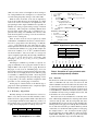
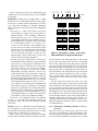
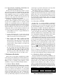
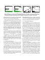
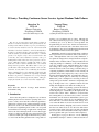
R-Sentry: Providing Continuous Sensor Services Against Random Node Failures
Shengchao Yu
WINLAB
Rutgers University
Piscataway, NJ 08854
[email protected]
Yanyong Zhang
WINLAB
Rutgers University
Piscataway, NJ 08854
[email protected]
Abstract
nectivity over a significant period of time. Although initial solutions have been proposed to provide coverage and
connectivity [11, 4, 19, 2], there is a severe problem– the
frequent failing of sensor nodes– that has received little attention. In sensor networks, due to the nature of the sensor
node hardware, there exists a fundamental tradeoff between
network lifetime and network service quality.
Maintaining graceful operations under faulty conditions
has long been a focus of research in other resource-rich systems. Although failures cannot be totally eliminated , a
few practical strategies have emerged and been adopted to
limit the effects of failures. These strategies usually involve
employing backups or redundancy to smoothly transfer the
load once a failure occurs. Though effective in resourcerich settings, these strategies can not be applied to sensor
networks because of the severe energy constraints, the poor
computing capabilities, and the nature of radio circuitry. In
particular, many radios employed by today’s sensor nodes
have the unfortunate failing that, even when idle, they consume nearly as much power as when they are receiving.
Further, the power consumption for receiving is almost as
taxing as the power needed to transmit. Consequently, turning on backup nodes is not a prudent solution since the
backup node might not even outlive the working node.
In order to build a long running system from relatively
short-lived sensor nodes, a widely-adopted approach is to
include high degree of redundancy in the deployment, and
let the nodes work in “shifts”. Therefore, at any moment,
the working shift (i.e., the active nodes) consists of a minimal number of nodes needed to maintain the system’s operations, while the rest of the nodes (i.e., the redundant nodes)
have their radios off. The downside of this strategy, however, is that the failure of an active node will lead to a hole
in the network, thereby disrupting sensor services. Even in
the ideal case where nodes do not die before their batteries drain out, the death of an active node still could disrupt
the services since network dynamics make it impossible to
precisely predict when power resources will be depleted.
In this paper, we propose R-Sentry, a node scheduling
algorithm that attempts to balance continuous network ser-
The success of sensor-driven applications is reliant on
whether a steady stream of data can be provided by the underlying system. This need, however, poses great challenges
to sensor systems, mainly because the sensor nodes from
which these systems are built have extremely short lifetimes.
In order to extend the lifetime of the networked system beyond the lifetime of an individual sensor node, a common
practice is to deploy a large array of sensor nodes and,
at any time, have only a minimal set of nodes active performing duties while others stay in sleep mode to conserve
energy. With this rationale, random node failures, either
from active nodes or from redundant nodes, can seriously
disrupt system operations. To address this need, we propose R-Sentry, which attempts to bound the service loss duration due to node failures, by coordinating the schedules
among redundant nodes. Our simulation results show that
compared to PEAS, a popular node scheduling algorithm,
R-Sentry can provide a continuous 95% coverage through
bounded recoveries from frequent node failures, while prolonging the lifetime of a sensor network by roughly 30%.
Keywords:
Sensor Networks, Network Coverage, Fault Tolerance,
Node Failure, Gang
1. Introduction
Sensor networks promise to change the way we interact
with the physical world: instead of querying data as a response to events, sensor networks continuously push data to
applications so that necessary parsing and analysis can take
place before events occur. The very fact that this data may
be collected for significant periods of time over vast spatial
areas facilitates a broad range of applications. An important
issue for the successful deployment of sensor-driven applications is to make sure that the sensor network will be able
to deliver as much spatio-temporal information as possible,
i.e. sensor networks must guarantee both coverage and con-
Figure 1. Illustration of a WSN.
vices and extended network lifetime in the presence of frequent node failures. For every active node, R-Sentry groups
the nodes whose sensing/networking functionalities overlap
with that of the active node into gangs. A gang consists of
a set of redundant nodes that can collectively replace the
active node upon its failure. R-Sentry ensures that, every
so often, a gang will wake up to probe whether the active
node is still functioning. If a failure has occurred to the active node, the probing redundant nodes can become active to
take over the failed active node to resume network services.
Hence, R-Sentry promises to limit the service loss time by
coordinating the wake up schedules of the redundant nodes.
R-Sentry also seamlessly handles more complicated situations, such as cases where a redundant node serves multiple active nodes simultaneously, or cases where redundant
nodes die before the active node fails.
Compared to existing techniques that share the same
viewpoint of having redundant nodes sleep for periods of
time to conserve energy, such as PEAS [16] or OGDC [19],
R-Sentry takes a much closer look at the problem of local
network recovery in the face of node failures. It tries to
provide quality of service guarantees to sensor applications
instead of the best effort approach by using random wake
ups. We have conducted a set of simulation experiments
to study the performance of R-Sentry. Compared to PEAS,
R-Sentry can (1) provide a longer network life, (2) provide
better network coverage (> 95%), (3) provide controllable
coverage recovery, (4) provide more robustness against random node failures, and (5) provide better scalability with
larger node density.
The rest of the paper is organized as follows. We provide an overview of our sensor network model in Section 2,
followed by related work. In Section 4, we discuss the RSentry algorithm in detail. We present our simulation effort
and the simulation results in Section 5. We conclude in Section 6.
2. Sensor Network Model
In this section, we discuss in detail our wireless sensor
network (WSN) model.
2.1. Generic Sensor Network Model
Coverage: In this work, we adopt the grid-based coverage
model [11, 12] illustrated in Figure 1. In this popular cover-
age model, the square network field in question is imaginarily partitioned into grids, marked by the dotted lines in the
figure. The grids should be small enough so that the underlying physical phenomena do not exhibit much variability
within a grid. The grid points that fall within a node’s sensing area are considered covered by that sensor node. This
discretization approach simplifies the measurement of the
coverage, making the network coverage percentage equivalent to the percentage of the grid points that are covered.
This model can be enforced by having nodes exchange the
list of grid points it can cover with their neighbors, which
we call GridList. Figure 1 shows such a scenario where
there are a subset of sensor nodes, represented by darker
solid circles, actively monitoring corresponding grid points,
while other nodes are not required for the coverage under
the model. With sufficient node density, there is a high
probability that, out of uniformly randomly deployed nodes,
there exists a set of nodes that could collectively cover all
the grid points in the network field.
Connectivity: In addition to sensing the physical world, a
WSN is also responsible for delivering the sensed data to
the applications. Network connectivity thus requires that
there exists a routing path between every sensing node and
the sink. In order to achieve this goal, it may be necessary to have more active nodes than just those needed for
provide sensor coverage, i.e., we may need extra nodes to
have good network connectivity, which are represented by
the light solid circles in Figure 1.
To focus on failure recovery schemes, we choose grid
sizes small enough to ensure connectivity through coverage: a WSN that satisfies the coverage requirement is automatically connected. This was also observed in many earlier studies [16, 4, 11], which assumed the communication
range is at least double of the sensing range. Therefore, in
this paper, we can focus on providing sensing coverage.
Turning Off Redundant nodes: Energy is a scarce resource for many sensor nodes may not have external power
sources, and have to rely on batteries. Even a battery with a
capacity of 3000 mA-hour can only last for 17 months [3].
A sensor node has three main components: sensor(s), processor, and radio. Sensors measure physical phenomena,
the processor takes as input the data from the sensors or the
network and performs in-network processing, while the radio communicates with the rest of the network. Among the
three, the radio is by far the main power consumer [17]. For
example, a Mica2 radio has current draw of 12mA in transmitting and 8mA in receiving. It’s worth noticing that a radio being in receiving mode does not necessarily mean the
application is receiving any valid packets; it is merely monitoring the medium. The energy consumed by a Mica2 radio in transmitting a 30-byte message is roughly equivalent
to the energy consumed by an ATMega128 processor exe-
cuting 1152 instructions [9]. As a result, if we leave all the
sensor nodes on, then no matter how many are deployed, the
network cannot function longer than 17 months. In practice,
to extend network lifetime it is necessary to have redundant
nodes off and turn them back on only when needed.
Disruptions Caused by Node Failures: Although the strategy discussed above is energy-conscious, it does not provide any robustness against random node failures. For instance, suppose that grid point p was monitored by sensor
node s while all the other nodes that can also cover p were in
sleep mode. Further, suppose that those sleeping nodes will
wake up at a later time t. If s fails at time t0 , then during this
period with duration t−t0 , the coverage and/or connectivity
of the network will be lost. In particular, node failures will
occur more frequently under heavy traffic volumes, which
is more likely when the monitored physical phenomena exhibit interesting behavior. Fail to collect or forward data on
these occasions can have severe consequences, likely detrimental to the applications.
2.2. Target Sensor Network Assumptions
In this study, the WSNs have the following features:
Regularity in Sensing and Communication. The popular
disk sensor model [11, 10, 16] is used to simplify the analysis and simulations. Specifically, a node’s sensing area is
a circular disk with the node as the center and the sensing
range as radius; and the neighbor nodes that fall into the
cocentric circle with the transmission range as radius are
considered as 1-hop neighbors. Moreover, all the links are
symmetric.
Resource-constraints. Sensor nodes are battery-driven and
non-rechargeable, except the sink node.
Location-Awareness. Each sensor node is assumed to be
stationary and have its own location, which can be obtained
through either localization devices, such as GPS, or certain
localization algorithms [7, 8]. We further assume the sensor
nodes have the geographical location of the network field in
which they are deployed. Based on a node’s location and
sensing radius, it can obtain the list of grid points it covers.
3. Related Work
Local networking repair has been studied in the context
of sensor networks, and several strategies have been proposed, such as GAF [14], AFECA [13], and ASCENT [1].
GAF identifies those nodes that are equivalent in terms of
routing capabilities, and turns them off to conserve energy.
In AFECA, a simple adaptive scheme is employed to determine the node sleep interval for those nodes that are turned
off. ASCENT shares the same goal as GAF, and it also considers mechanisms for sleeping nodes to come back and join
the routing when necessary. To avoid degrading connectiv-
ity severely, sleeping nodes need to wake up relatively frequently. In addition, a fixed sleep interval is used for every
node in the network. The authors also proved that the upper
bound on the lifetime improvement is the ratio of a node’s
sleep interval to its awake period.
Besides information delivery, data collection is the other
critical task of sensor networks. In PEAS [16], an independent probing technique was proposed for redundant nodes
to check whether there is an active node in its vicinity.
OGDC [19] is a round-based node scheduling algorithm
which selects active nodes based on their geo-locations to
improve network lifetime. In [5, 15], all the nodes that can
cover the same spot form a cluster, and at any time, there is
only one active node from the cluster while the other members stay in the sleep mode.
Compared to the aforementioned earlier work, R-Sentry
takes a closer look at the problem of local network recovery
in the face of node failures, and takes a distinctly different
approach: (1) R-Sentry tries to provide quality of service
guarantees to sensor applications instead of using a best
effort approach based on random wake ups; (2) the wake
ups of the redundant nodes are carefully scheduled to ensure timely network recovery with less energy consumption,
and (3) waking up one redundant node to replace the failed
active node is often impossible. R-Sentry extends our exploratory work in [18] by introducing the concept of gangs
and conducting more comprehensive evaluations.
4. The Design of R-Sentry
While on duty, a WSN is composed of two types of
nodes: active nodes , which are performing duties; and
redundant nodes, which are sleeping with their radios off.
While active nodes is on duty, the redundant nodes should
not sleep for an infinitely long period. Rather, they should
wake up from time to time and check the conditions of the
active nodes. Every node randomly waking up [16, 1], however, is wasteful and does not provide much benefit. For instance, if the subsequent wake ups are far apart from each
other, then it is impossible to ensure quick network recovery. To address this void, we propose a coordinated scheduling algorithm among all the redundant nodes. Those redundant nodes that wake up play a role analogous to sentries in
real world in the sense that they monitor the health of the active node, and whenever a fault or failure occurs, they jump
in to replace the lost node. In the following discussions,
we use redundant node and sentry interchangeable. Since
redundant nodes rotate to wake up, we call this scheme Rotatory Sentries or R-Sentry.
4.1. Redundant Sets and Gangs
Before going into details of R-Sentry, it is beneficial to
examine the redundancy among nodes. Every sensor node
has a group of neighbor nodes with overlapping communication or sensing capabilities. The sensing redundant set
(SRS) of a node consists of its neighbors whose sensing areas overlap with the node’s sensing area, i.e. nodes that can
cover the same grid point(s) belong to each other’s SRS.
When an active node fails, it can only be replaced by
nodes from its SRS. However, the replacement of a failed
active node can not necessarily be accomplished by simply replacing it with a single redundant node, regardless of
whether one is trying to repair sensing coverage or network
connectivity. This viewpoint is distinctly different from
those in earlier studies such as [16, 1], which tried to replace the active using one redundant node. In fact, it has
been shown in [4] that on average 3-5 nodes are needed to
replace a node’s sensing area.
Since an active node can only be replaced by certain
combinations of redundant nodes, there is a need for the active node to group all the nodes that belong to its SRS into
“gangs”. Nodes that belong to the same gang can collectively replace the active node. Now let us look at an example
to understand the definition of a gang. In this example, the
active node A’s SRS is {B, C, D, E, F }, and their GridLists
are shown in Table 1. We can see that A’s coverage area
can be completely replaced by the following combinations:
{B}, {C, D}, {C, E}, and {D, E, F }. As a result, A has
four gangs: {{B}, {C, D}, {C, E}, {D, E, F }}, which we
call GangList.
One thing we would like to point that is, a superset of a
gang set technically is also a gang. For instance, in the example in Table 1, the set {B, C} is also a gang. However, in
this paper, we only focus on “minimum gangs”, those sets
that would no longer be a gang should we remove any member from the set. Grouping nodes from an SRS into gangs
is essentially a combinatorial problem. shows the pseudo
code for a node populating its GangList with gangs of sizes
no larger than gs. In order to limit the computation of this
procedure, we only consider gangs of small sizes.
For the purpose of fault tolerance, nodes that belong to a
gang need to wake up simultaneously to completely replace
the functionalities of an active node.
4.2. R-Sentry Algorithm
R-Sentry attempts to bound the duration of service loss.
That is, every time an active node fails, R-Sentry seeks to
make nodes from a gang available within a time interval of
∆ (an example schedule shown in Table 3(b)), where ∆ is
the promised service loss time limit. If an active node has
N gangs, then each gang needs to wake up every N ∆.
node ID
A
B
C
GridList
{1, 2, 3, 4}
{1, 2, 3, 4, 5}
{1, 2, 3, 5}
node ID
D
E
F
GridList
{1, 4, 5, 6, 7}
{3, 4, 5, 6, 8}
{2, 9, 10}
Table 1. An example of GridList table.
GENE-GANGS(SRS, gs)
// gs : maximum gang size
1 i = 1; clear GL;
// GL : Gang List
2 GCL = SRS;
// GCL : Gang Candidate List
3 while i ≤ gs
4
clear TEMP GCL;
// TEMP GCL : temporarily GCL
5
for each set s in GCL
6
if s is a minimum gang
7
then push back s to GL;
8
else push back s to TEMP GCL
9
if i < gs
10
then GCL = PREPARE-CANDY(TEMP GCL);
11 return GL
PREPARE-CANDY(TEMP GCL)
1 clear GCL;
2 for each set t in TEMP GCL
3
for each node srs in SRS
4
t = srs ∪ t;
5
push back t to GCL;
6 return GCL
Table 2. Algorithm for generating gang
Gang
{B, C}
{D, C, E}
{B, E}
{E, F }
Time To Wake Up (s)
1200
1500
1800
2100
(a) Gang schedule table
B
C
D
C
E
B
E
E
F
B
C
D
C
E
B
E
E
F
B
C
1200
1500
1800
2100
2400
2700
3000
3300
3600
Time (s)
(b) Wake up schedule
Table 3. Illustration of a gang schedule table
and the resulting wake up schedule.
4.2.1 Basic idea
The discussions in this section have simplified assumptions
such as a redundant node only serves one active node, and
all the redundant nodes will not fail before the active nodes
do. We made these assumption to keep the explanation easy
to understand, and in the following sections, we discuss how
to extend R-Sentry to handle more realistic scenarios, where
a redundant node may belong to multiple active nodes, and
node failures can occur at random times.
We let the active nodes maintain most of the data structures, while having redundant nodes only keep track of their
own next wake up time. The most important data structure maintained by an active node is its gang schedule table,
which specifies each gang’s next wake up time. An illustration of such a data structure is provided in Table 3(a). Based
on this table, we can infer the wake up times for each gang.
For example, with ∆ = 300s, if an active node has 3 gangs,
the gang that wakes up at time 1200s also wakes up at times
2100s, 3000s, 3900s, etc. Therefore, a portion of the wake
up events caused by Table 3(a) is shown in Table 3(b).
Next we discuss how active nodes establish their gang
schedule tables, and more importantly, how they maintain
the schedules.
Initialization: During the bootstrapping phase, a WSN
usually runs a host of initialization services, such as neighbor discovery, localization, time synchronization, route discovery, duty-cycle scheduling, etc. Similarly, a WSN that
employs R-Sentry needs the following extra initialization
services:
• Gang Discovery. This service ensures every sensor
node identifies its neighbor nodes, and populates its
SRS and GridList. At the beginning, each node in
the network sends out a presence announcement message including its ID and location . Such messages are
flooded within h hops around the source nodes, where
h is a small number, usually 1 or 2, as the presence
announcement only matters to nodes within the vicinity of the source node. After a certain amount of time
in the process, every node will receive the announcements from all of its SRS members, based on which
a node can calculate the GridList of each node in its
SRS. After that, a node would be able to form its own
GangList in the way illustrated in Table 2.
A
active
G D BC
up up up
C
up
B
up
F
up
E
up
Time (s)
1200
1300
1400
1500
1600
1700
1800
(a) The events that have been observed by A.
{B, C}
{D, E}
{E, F}
-
(b) t = 1200
{B, C}
{D, E}
{E, F}
1600
-
{B, C}
{D, E}
{E, F}
1600
1900
-
{B, C}
{D, E}
{E, F}
2200
1900
2500
(d) t = 1400
(f) t = 1550
(h) t = 1700
{B, C}
{D, E}
{E, F}
1600
-
{B, C}
{D, E}
{E, F}
1600
-
{B, C}
{D, E}
{E, F}
2200
1900
-
{B, C}
{D, E}
{E, F}
2200
1900
2500
(c) t = 1300
(e) t = 1500
(g) t = 1600
(i) t = 1800
Figure 2. Illustration of how a new active
node establishes its gang schedule table.
• Schedule Bootstrapping. The initial set of active nodes
are determined by the underlying coverage and initialization protocols. Our approach is similar as the one
employed in CCP [11], which can be broken down
into 3 steps: 1) after presence announcement exchange
phase, every node stays active and starts a random
backoff timer, collecting redundancy announcement
from its SRS members; 2) upon the timer’s expiration,
a node checks its SRS members’ redundancy status and
determines if all grid points in GridList are covered by
the non-redundant SRS members. If yes, it considers
itself redundant and broadcasts redundancy announcement, otherwise it considers itself non-redundant and
doesn’t take any actions; 3) at the end of bootstrapping
phase, the non-redundant nodes calculate their gangs’
schedules and flood them within a small number of
hops, staying active; while the redundant nodes, upon
receiving the schedules, record their own wake up time
or the earliest one if it receives multiple schedules.
At the end of the initialization phase, the redundant
nodes go to sleep with their sleep timers properly set
up, while the active nodes start collecting and forwarding
sensed data.
the other sentries of the same gang will also wake up and
probe. If the target active node is still alive, it will match
the node ID’s contained in the probing messages with the
gang whose scheduled wake up time is closest to the current
time. If the match is successful, the active node updates the
gang schedule table by incrementing the wake up time by
the round duration N ∆. Finally, the active node sends the
sentries a reply message which has two fields: NextWakeTime, and CurrentTime. The CurrentTime field is used to
synchronize the clocks between the sentry nodes and the
active node.
The above discussion assumes the active node is still
alive while sentries probing. If the active node has failed
before sentries probe, the sentries will not receive the reply
message, then they conclude the active node has failed. In
this situation, the sentries should become active to provide
uninterrupted services. The design of R-Sentry thus ensures
that, whenever one of the active node fails, its functionality will be fully resumed by other nodes roughly within ∆,
when the sentries outlive the target active node and corresponding communication time is negligible compared to ∆.
Therefore, R-Sentry can limit the service loss period within
a tolerable threshold.
Probing: A sentry (i.e. redundant) node periodically wakes
up, as scheduled, to probe the active node. If the active
node has failed, sentry nodes will become active to resume
network services; otherwise, they go back to sleep.
When a sentry node wakes up, it broadcasts a probing
message with its node ID included. Around the same time,
4.2.2 Dynamically establishing schedules for new active nodes
After the sentry nodes become active, these new active
nodes face several challenges. The main challenge stems
from the fact that the communication between the new active node and the redundant nodes that belong to its SRS
has not been established. On one hand, the redundant nodes
are still following the schedules of the previous active node,
without realizing that the active node has changed. On the
other hand, the new active node does not have a schedule for
its gangs, and therefore, it will not be guarded properly. Further complicating the problem is that it is impossible for the
new active node to communicate with the redundant nodes
when they are asleep for their radios are off. As a result,
we can only attempt to establish the schedule gradually as
more and more redundant nodes wake up in groups down
the stretch.
The algorithm a new active node uses to establish its
schedule is rather simple, yet effective. The idea is that,
if the redundant node that is probing is not associated with
a wake up time in the gang schedule table, the new active
node will assign the next available wake up slot to the gang
that contains this redundant node. If the node is included in
multiple gangs, the smallest gang will be picked.
To better understand this algorithm, let us walk through
an example shown in Figure 2. Suppose node A is the new
active node, and its GangList is {B, C}, {D, E}, and {E,
F}. The ∆ is 300 seconds. Figure 2(a) illustrates the wake
up events A observes in the establishing phase, and for each
event, it shows the corresponding schedule table in the subsequent figures (Figures 2(b-i)). In particular, the establishing phase has the following steps:
1. A becomes active at time 1200, when A’s schedule is
empty (Figure 2(b)).
2. At time 1300, B wakes up. A then assigns next available wake up slot, i.e. the current time incremented by
∆, 1600, to gang {B, C}, and updates the gang schedule table accordingly (Figure 2(c)).
3. At time 1400, C wakes up. A finds C is already scheduled, so it does not update the gang schedule table. It
just simply sends a reply message to C to instruct C to
wake up at 1600 (Figure 2(d)).
4. At time 1500, G wakes up. A finds G does not belong
to its SRS, so it does not update the gang schedule table. A sends a reply message to G with a large sleep
interval (Figure 2(e)). If G serves other active nodes,
it will receive a much shorter sleep time from them.
5. At time 1550, node D wakes up. A assigns next available wake up slot, 1900, to gang {D, E}, and updates
the gang schedule table accordingly (Figure 2(f)).
6. At time 1600, node B and C wake up according to the
schedule. Since A’s table is not fully occupied yet, A
assigns the next available wake up slot, 2200, to them
(Figure 2(g)).
7. At time 1700, node F wakes up. A assigns the next
available wake up slot, 2500, to node E and F (Figure 2(h)).
{B, C}
{D, E}
{F, G}
1200
1500
1800
{B, C}
{D, E}
{F, G}
3000
2400
2700
(a) t = 1000
(c) t = 2400, A still has not
heard from D.
{B, C}
{D, E}
{F, G}
2100
1500
1800
{B, C}
{F, G}
3000
2700
(b) t = 1500
(d) t = 2400, A cleans up its
gang schedule table
Figure 3. An example illustrating how a active node detects failures among redundant
nodes and adapts its schedule accordingly.
8. At time 1800, node E wakes up. A does not update
the schedule table because E is already scheduled. A
sends a reply message to E, requesting E to wake up
at time 1900 (Figure 2(i)).
9. After that, A becomes a normal active node, and it will
handle the subsequent waking sentries by incrementing their wake up times by 3∆ = 900.
We note that a new active usually can establish its gang
schedule within a reasonable amount of time because according to R-Sentry, every redundant node wakes up periodically, and this period will be the upper bound of the time
taken to form the schedule.
4.3. Scheduling Redundant Nodes That
Serve Multiple Active Nodes
To simplify the discussion, we assumed that a redundant
node only serves one active node in the earlier sections.
In this section, we look at how R-Sentry handles the cases
where a redundant node may serve multiple active nodes.
If a sentry node guards multiple active nodes, the main
challenge lies in that when it probes, how it handles schedules from multiple active nodes. In R-Sentry, when a sentry
node probes, it only includes its own ID in the probing message. Each of the active nodes that receive the probing messages, will examine the difference between the scheduled
wake up time of that redundant node and the current time
at the active node. If the difference is below a threshold,
the corresponding active node assumes this is a valid wake
up, calculates its next wake up time, and sends a reply message back. The reply message contains three fields: the next
wake up time Tnext , the current time Tcurr , and the active
node’s ID. Those active nodes that have a different wake up
time for the redundant node will simply copy the previously
scheduled wake up time to the reply message. After receiving all the reply messages, the redundant node calculates
the sleep interval for each of the active nodes, chooses the
shortest one as the next sleep interval , and synchronizes its
clock appropriately.
4.4. Dynamically Adjusting Schedules for
Missing Redundant Nodes
In many sensor network applications, failures occur not
only to active nodes, but also to redundant nodes, even when
they are in sleep mode. For instance, a catastrophic event,
such as lightning can cause sensor node failures, regardless
of their state. When a redundant node fails, the active node
cannot rely on the gangs that contain the failed node, and
should remove these gangs from its schedule.
In R-Sentry, dynamically adapting the active node’s
schedule is rather straightforward. If the active node does
not hear from a redundant node in k consecutive rounds
(usually, k is a small number such as 2), it simply removes
the gangs that contain the missing node from the gang list.
In order to understand the details, let us look at an example
illustrated in Figure 3, where the active node A has the following gangs, {B, C}, {D, E}, and {F, G}; and the ∆ is 300
seconds. Node D fails at time 1000. What happens to A is:
1. At time 1000, node D fails. A’s gang schedule table is
shown in Figure 3(a).
2. At time 1500 (Figure 3(b)), A only receives probes
from E, not D. A decides to wait for one more round
(900 seconds in this case) before taking actions.
3. After a round, at time 2400, A still has not heard
from D (Figure 3(c)). A then concludes that D has
failed, and removes the gang {D, E} from the schedule
(shown in Figure 3(d)). At this time, A will still send
a reply message to E that includes a reasonably long
sleep time, like 2∆.
4. A will schedule the remaining two gangs as usual, with
the only exception that the round duration now becomes 600 seconds. As a result, gang {B, C} will wake
up at times 3000, 3600, 4200, etc, while gang {F, G}
will wake up at times 2700, 3300, 3900, etc. Therefore, A will still receives probes every 300 seconds.
5. Performance Evaluation
In this section, we first define a simplified sensor failure
model, then give the simulation model and simulation setups. After that we examine R-Sentry’s performance against
PEAS, in terms of scalability, energy efficiency, service
availability, coverage recoverability and fault tolerance.
5.1. Sensor Failure Model
We purposely introduce sensor failures into our simulations to model the fact that random node failures are norms
instead of exceptions in sensor network. The catastrophic
failure model used in our simulation is a coarse-grained
model, in which a percentage of sensor nodes that are alive
(but not necessarily active) “die” due to external catastrophic events, like natural disasters. By “die”, we mean the
node stops functioning completely as an electronic device,
even though it’s possible in reality that not all components
in the node are affected by the external events.
This failure model has two parameters: (i) failure period fp , the mean time between consecutive external catastrophic events (the intervals between two events are random
numbers that follow an exponential distribution), and (ii)
failure percentage f% , the mean percentage of the live nodes
that are affected by a particular event. Upon a catastrophic
event, the actual percentage of affected nodes is a random
number between 0 and 2f% .
5.2. Overview of PEAS
In this study, we compare R-Sentry’s performance
with PEAS [16], a well-recognized fault-tolerant energyconserving protocol for sensor networks. Before we present
the detailed simulation results, we would like to first give a
brief description of PEAS. Like R-Sentry, PEAS also assumes that at any moment, only a subset of nodes stay active, while the others go to sleep and wake up periodically
to probe the health of the active node(s). PEAS, however,
allows the redundant nodes to independently wake up, without coordinating the schedules among them, and as a result,
it only provides a coarse granularity of fault-tolerance.
PEAS guarantees there is at least one active node within
every redundant node’s probing range. An active node controls the wake up frequencies of the redundant nodes using
the parameter λd , the desired probing rate. Every time an
active node receives a probing message, it replies with λd
b that it has observed, based on
and the actual probing rate λ
which the probing node calculates its new probing rate as
λnew = λold λd . Then the probing node generates its new
b
λ
sleep interval ts following the probability density function
new
f (ts ) = λnew e−λ ts . We note that, in PEAS, the parameter 1/λd is similar to ∆ in R-Sentry, both denoting the desired recovery time from the applications, and we use these
two notations interchangeably when presenting the results.
5.3. Simulation Model and Settings
We have implemented both R-Sentry and PEAS on our
own simulator USenSim. USenSim is a discrete event-driven
simulator that is intended to model large-scale sensor networks. In order to realize the network scale we envision, i.e.
with thousands of nodes, which was impossible with more
detailed network simulators such as NS-2, USenSim assumes a constant transmission delay between nodes and serialized transmissions among nodes that compete the channel, similar as the one adopted in [11]. We believe the simRouting protocol
Communication range
Receiving power
Sleeping power
Bandwidth
Shortest path
15m
0.012w
0.00003w
20Kbps
Sensing range
Transmission power
Idle power
Sensing power
Packet size
10m
0.06w
0.012w
0.001w
25Bytes
Table 4. Simulation Platform Parameters
Coverage
# of Active Nodes
20
0
0
60
40
Coverage
# of Active Nodes
20
1
2
3
time (seconds)
(a)
4
4
x 10
0
0
1
2
3
time (seconds)
(b)
4
4
x 10
600
6
500
5
90% lifetime(seconds)
40
80
percentage(%)
percentage(%)
80
60
PEAS
100
average coverage loss time(seconds)
R−Sentry
100
400
300
200
100
0
0
R−Sentry
PEAS
100
200
300
400
delta (seconds)
500
600
4
x 10
4
3
2
1
0
0
(c)
R−Sentry
PEAS
100
200
300
400
delta (seconds)
500
600
(d)
Figure 4. Network coverage statistics throughout the lifetime of a WSN: (a) R-Sentry, and (b) PEAS.
The average coverage loss time and the 90% network life time with ∆ are shown in (c) and (d).
plified network model does not prevent us proving the validity and effectiveness of our algorithm, given that our work
is orthogonal to the works in the underlying layers.
Unless specified, the simulation setup has 600 sensor
nodes uniformly randomly deployed in a 50×50m2 square.
Each grid is a 1 × 1m2 square. The initial energy of a sensor node is uniformly distributed between 50 and 60 Joules,
which allows the node to function around 4000 ∼ 5000 seconds if the radio is in idle listening mode. Every 50 seconds, each active node transmits a packet containing collected data to the sink, which is located at the center of the
field and has persistent power supply. The neighbor nodes
that are located within the distance of 15m constitute SRS.
Due to the high redundancy, a gang size of 1 is sufficient in
the simulations.
For those parameters that are specific to PEAS, we have
tried various parameter values, and chosen the following
settings because they produced the best results: probing
range Rp = 3m, desired probing rate λd = 0.02, initial probing rate λs = 0.02, and k = 32. We would like
to emphasize that we chose a rather small probing range
for PEAS to guarantee all the grid points are covered since
PEAS does not explicitly require every grid point to be covered. The network/energy parameters used in our simulations are summarized in Table 4, and we took these values
from PEAS [16].
5.4. Performance Metrics
Coverage ratio is the percentage of the grid points that
are covered at a time. Both R-Sentry and PEAS attempt
to achieve a high coverage ratio throughout their lifetimes.
β network lifetime is the duration the network lasts until the coverage ratio drops below β and never comes back
again. We use β lifetime to measure the protocol’s capabilities of preserving coverage and recovering coverage loss
from node failures.
Coverage loss time is the duration from when a grid point
loses coverage to when the coverage recovers. The average
coverage loss time reflects how quickly a failed active node
can be replaced by the redundant nodes.
Packet delivery ratio is the ratio of number of packets received by the sink to the number of packets sent out by the
active nodes in a specific length of time window. The packet
delivery ratio indicates the connectivity of the network.
5.5. Performance Results
Service Availability: The motivation behind this study is
the need to provide uninterrupted services throughout a sensor network’s lifetime. Figures 4 (a) and (b) shows how the
coverage ratio evolves with time for the two schemes. In
this experiment, we have ∆ = 50 seconds in both schemes.
We observe that R-Sentry can offer a 95% coverage ratio
until 2.5 × 103 seconds, while PEAS’s coverage ratio drops
below 90% from 2.5 × 103 seconds. This is because in RSentry, once an active node fails, it can be quickly replaced
by a gang, while in PEAS, there is not a guarantee that the
awake redundant node can fully replace the active node.
We can also confirm our hypothesis by looking at the
time series of the percentage of active nodes in both cases.
R-Sentry can maintain a steady number of active nodes,
which can in turn guarantee a high coverage ratio, but in
PEAS, the number of active nodes decreases with time due
to oversleeping. We note that the drop of the number of active nodes in PEAS around 5000 second is due to the fact
that most of the initial active nodes failed at that time. We
did not observe a drop in R-Sentry because it can quickly
recover from failures.
Algorithm Controllability: Controllability is a valuable
feature for an algorithm, in that the performance of an algorithm with controllability can be easily tuned up to match
application requirements. In this set of experiments, we varied ∆, and collected the corresponding average coverage
loss time , which is shown in Figure 4(c). We can observe
that R-Sentry demonstrates good controllability: for any
given ∆ value, the resulting average coverage loss time is
always below ∆, and often slightly higher than ∆/2. PEAS,
however, fails to do so – we cannot correlate the delivered
coverage loss time and the desirable coverage loss time.
Thanks to the capability of maintaining high coverage ratio and low coverage loss time, R-Sentry can make the sen-
4
400
3.5
350
300
R−Sentry
PEAS
250
200
150
100
3
2.5
2
1.5
1
R−Sentry
PEAS
0.5
50
0
1000
2000
3000
4000
5000
6000
failure period (seconds)
7000
0
0
8000
2000
4000
6000
failure period (seconds)
(a)
8000
(b)
5
600
R−Sentry
PEAS
500
90% lifetime(seconds)
450
4
x 10
average coverage loss time (seconds)
4.5
90% lifetime(seconds)
average coverage loss time (seconds)
500
400
300
200
100
0
0
5
10
15
failure percentage (%)
(c)
20
4
x 10
R−Sentry
PEAS
4
3
2
1
0
0
5
10
15
failure percentage (%)
20
(d)
Figure 5. The impact of fp on average coverage loss time and 90% network lifetime is shown in (a)
and (b) (with f% = 5%, and ∆ = 50 seconds). The impact of f% on average coverage loss time and
90% network lifetime is shown in (c) and (d) (with fp = 5000 seconds, and ∆ = 50 seconds).
14
4
x 10
10
8
6
4
2
4
x 10
14
90% lifetime(seconds)
90% lifetime(seconds)
16
R−Sentry
PEAS
12
12
R−Sentry G1
R−Sentry G5
PEAS G1
PEAS G5
10
8
6
4
2
0
0
500
1000
node number
(a)
1500
2000
0
0
500
1000
node number
1500
2000
(b)
Figure 6. Scalability and impact of grid size
sor network function for a much longer period, as shown in
Figure 4(d). The interesting phenomenon we observe from
Figure 4(d) is that the 90% network lifetime stays almost the
same as ∆ goes up. This can be explained by the fact that,
though a large ∆ can save more energy by making redundant nodes sleep longer, the likelihood of the overall coverage ratio falling below a certain percentage (90% in this
case) is also higher due to oversleeping. As a result, these
two effects will cancel each other.
Fault Tolerance: It’s not unusual that sensor nodes die before running out of energy [6, 16, 1]. In this set of experiments, we evaluate the robustness of the two schemes
against node failures under the catastrophic failure model.
In Figures 5(a) and (b), we fixed f% as 5%, and varied
the value of fp . Since R-Sentry has sentry nodes guarding
active nodes and can dynamically adapt an active’s node
schedule table to accommodate the failures of its redundant
nodes, it is rather robust against random node failures. Figure 5(a) shows that, regardless of the failure rate, R-Sentry
is able to replace a failed active node around 50 seconds
(which is the value of ∆). On the other hand, in PEAS,
the average service loss period is much longer. As a result,
R-Sentry provides a much better 90% network lifetime than
PEAS across all the failure rates (shown in Figure 5(b)). We
also observe the similar trend from the results when we fix
fp but vary f% , which are shown in Figures 5(c) and (d).
Energy Efficiency and Scalability: Many sensor applications seek to achieve longer network lifetime by deploying
more nodes. Therefore, the ability to translate a larger number of sensor nodes into a prolonged network lifetime is
critically important to node scheduling algorithms like RSentry and PEAS. In this set of experiments, we varied the
number of sensor nodes, and measured the resulting 90%
lifetime. The results, reported in Figure 6(a), show that
R-Sentry leads to longer lifetimes than PEAS by roughly
30%. This is because R-Sentry maintains a good coverage
ratio for a much longer duration than PEAS through careful
scheduling, which leads to a better 90% lifetime. In fact, we
find that the 90% lifetime in R-Sentry almost scales linearly
with the number of nodes, and that the difference between
the two schemes increases with the number of nodes.
Connectivity: Our simulations also show that, both algorithms achieve more than 95% packet delivery ratio during
90% lifetime, which confirms our claim in Section 2.1. Due
to space limitation, we didn’t include these plots.
5.6. Discussion
Energy Overheard of R-Sentry: The ability to timely
wake up appropriate redundant nodes ensures R-Sentry’s
fault-tolerance. However on the other hand, it also entails
additional energy overhead by requiring extra message exchanges between nodes. Assuming no packet loss, when a
redundant node wakes up, it will send out a probing message, and will receive n reply messages, where n is smaller
than the number of active nodes at the moment. To better
understand the overhead, let us next look at one example
scenario. We assume 2000 nodes and 1 × 1m2 grids, and
we further assume that each node on average wakes up 75
times during the 90% lifetime and receives 16 replies during each wake up (with a total of 1200 reply packets). According to our simulation traces, these numbers are rather
conservative. Given the power specifications in Table 4, the
amount of energy consumed in transmitting the aforementioned scheduling related packets would be:
(75 + 1200) ∗ (25 ∗ 8/20000) ∗ 0.06 = 0.765 Joules
which is less than 2% of the initial energy level. Therefore,
we take the viewpoint that the energy overhead of R-Sentry
is rather low.
The Impact of Grid Size: The grid is virtual, but its size
plays a role in R-Sentry: larger size usually leads to longer
lifetime since fewer active nodes are needed to cover all
the grid points, which we confirmed through experiments.
Specifically, we adopted two grid sizes: 1×1m2 , referred to
as G1 and 5×5m2 , referred to as G5. The results are shown
in Figure 6(b). We can see that the 90% network lifetime of
R-Sentry can be further improved by the system adopting
a larger grid size. In fact, a grid size of 5 × 5m2 extends
the lifetime by 30%. However, excessively large grid would
compromise connectivity since the network would be disconnected due to low density of active nodes. On the other
hand, since PEAS does not rely on the concept of grids, its
performance is not influenced by the grid size. We would
like to point out that the inconsistency between G1 and G5
in the case of PEAS is caused by artifacts of the simulations.
6. Concluding Remarks
Providing continuous, uninterrupted sensor services requires the network to be able to quickly recover from coverage loss due to frequent node failures. That is, if an active
node fails, its coverage should be quickly resumed by the
redundant nodes, which were sleeping to conserve energy.
Earlier node scheduling solutions, such as PEAS [16], adopt
completely random schedules among redundant nodes. A
random schedule cannot guarantee a redundant node will
wake up timely when the active node fails, nor can it guarantee the redundant node that happens to wake up can fully
recover the coverage hole.
R-Sentry addresses these issues by grouping redundant
nodes into “gangs”, which collectively can fully replace
an active node, and then by scheduling gangs with fixed
intervals. R-Sentry also takes into consideration realistic network situations, such as cases where a redundant
node serves multiple active nodes, or cases where redundant
nodes may fail before the active node. Through detailed
simulations, we show that R-Sentry can provide better resilience against failure while prolonging network life time.
As a result, R-Sentry has made a significant step towards
building reliable sensor services.
References
[1] A. Cerpa and D. Estrin.
ASCENT: Adaptive SelfConfiguring Sensor Networks Topologies. In Proceedings
of IEEE INFOCOM’02, June 2002.
[2] B. Chen, K. Jamieson, H. Balakrishnan, and R. Morris. Span:
An Energy-Efficient Coordination Algorithm for Topology
Maintenance in Ad Hoc Wireless Networks. In Proceedings
of ACM/IEEE MobiCom 2001, July 2001.
[3] CrossBow Technology.
Mote User’s Manual.
http://www.xbow.com/Support/Support pdf files/MPRMIB Series User Manual 7430-0021-05 A.pdf.
[4] Y. Gao, K. Wu, and F. Li. Analysis on the redundancy of
wireless sensor networks. In Proceedings of the 2nd ACM
[5]
[6]
[7]
[8]
[9]
[10]
[11]
[12]
[13]
[14]
[15]
[16]
[17]
[18]
[19]
international conference on Wireless sensor networks and
applications, pages 108 – 114, September 2003.
T. He, S. Krishnamurthy, J. A. Stankovic, T. Abdelzaher,
L. Luo, R. Stoleru, T. Yan, L. Gu, J. Hui, and B. Krogh. An
Energy-Efficient Surveillance System Using Wireless Sensor
Networks. In Proceedings of the ACM MobiSys 2004, 2004.
W. R. Heinzelman, A. Chandrakasan, and H. Balakrishnan.
Energy-Efficient Communication Protocol for Wireless Microsensor Networks. In Proceedings of the 33rd Hawaii International Conference on System Science, 2000.
K. Langendoen and N. Reijers. Distributed localization in
wireless sensor networks: a quantitative comparison. Comput. Networks, 43(4):499–518, 2003.
Z. Li, W. Trappe, Y. Zhang, and B. Nath. Robust Statistical
Methods for Securing Wireless Localization in Sensor Networks. In Proceedings of the IEEE/ACM IPSN’05, 2005.
S. Mohan, F. Mueller, D. Whalley, and C. Healy. Timing
analysis for sensor network nodes of the atmega processor
family. In Proceedings of the 11th IEEE Real-Time and Embedded Technology and Applications Symposium, 2005.
D. Tian and N. D. Georganas. A coverage-preserving node
scheduling scheme for large wireless sensor networks. In
Proceedings of the 1st ACM international workshop on Wireless sensor networks and applications, September 2002.
X. Wang, G. Xing, Y. Zhang, C. Lu, R. Pless, and C. Gill.
Integrated coverage and connectivity configuration in wireless sensor networks . In Proceedings of the ACM SenSys’03,
pages 28–39, November 2003.
G. Xing, C. Lu, R. Pless, and J. A. O’Sullivan. Co-Grid: an
efficient coverage maintenance protocol for distributed sensor networks. In Proceedings of IPSN’04, April 2004.
Y. Xu, J. Heidemann, and D. Estrin. Adaptive energyconserving routing for multihop ad hoc networks. Research
Report 527, USC/Information Sciences Institute, 2000.
Y. Xu, J. Heidemann, and D. Estrin. Geography-informed
Energy Conservation for Ad Hoc Routing. In Proceedings of
the ACM/IEEE MobiCom’01, July 2001.
T. Yan, T. He, and J. A. Stankovic. Differentiated Surveillance Service for Sensor Networks. In Proceedings of the
ACM SenSys’03, 2003.
F. Ye, G. Zhong, S. Lu, and L. Zhang. PEAS: A Robust Energy Conserving Protocol for Long-lived Sensor Networks.
In Proceedings of ICDCS’03, May 2003.
W. Ye, J. Heidemann, and D. Estrin. An Energy-Efficient
MAC Protocol for Wireless Sensor Networks. In Proceedings of IEEE INFOCOM’02, June 2002.
S. Yu, A. Yang, and Y. Zhang. DADA: A 2-Dimensional
Adaptive Node Schedule to Provide Smooth Sensor Network
Services against Random Failures. In Proceedings of the
Workshop on Information Fusion and Dissemination in Wireless Sensor Networks, 2005.
Honghai Zhang and Jennifer C. Hou. Maintaining sensing
coverage and connectivity in large sensor networks. Wireless
Ad Hoc and Sensor Networks: An International Journal, 1(12), January 2005.