Download User Manual

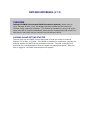
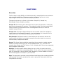
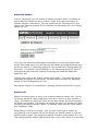
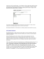
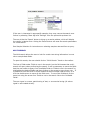
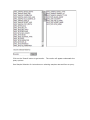
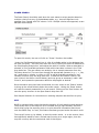
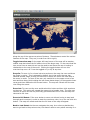
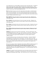
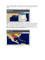
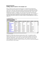
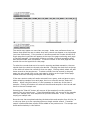
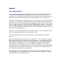
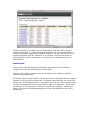
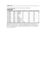
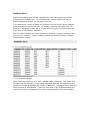
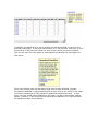
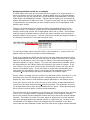
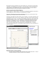
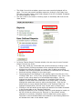
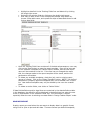
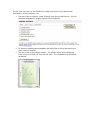
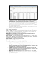
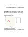
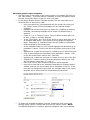
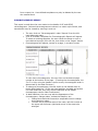
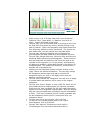
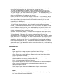
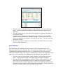
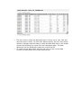
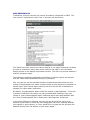
GWIS ENTERPRISE
Version 3.3
END-USER MANUAL
GWIS END-USER MANUAL (V. 3.3)
OVERVIEW
Infologic’s GWIS (Geochemical Web Information System) allows users to
store, manage, browse, view, and display geochemical data via the Internet or
Intranet, using a personal computer. This manual is intended for use by end-users—
those who wish to search the database, select specific samples/sites that result from
that search, and create various reports from the selected results.
LOGGING IN AND GETTING STARTED
The user may log into GWIS via any authorized PC that has access to Internet
Explorer 6.0 or later, or Firefox. Once GWIS is installed for a particular company, an
Internet address for GWIS will be provided to the user. The user’s company will
provide a user id and password, which are typed into appropriate boxes. Once the
user is logged in, the GWIS search options will appear’.
FUNCTIONS
Searches
The first step in using GWIS is to find the site and/or sample that the user wishes to
view or extract data from. There are a number of ways to perform a search,
depending on the user’s desired result and/or preference.
The search options can be found in the toolbar: Sample ID, Sample List,
Site/Sample, Power, Multiple, and Map.
Sample ID: This search option allows the user to search for samples in a range by
querying on the sample ID numbers. This method is useful if the user knows which
sample contains the desired data and is knowledgeable about as to what the
samples’ sample IDs are.
Sample List: This search feature allows the user to either search for samples by
range (just as in the Sample ID search), or to copy\paste a list of samples from a
report and view a list of samples matching those exact IDs.
Site/Sample: Site/Sample search is useful when the user wants to narrow the
search results by location or descriptive sample information based on commonly
used site and/or sample information.
Power: The Power Search should be used when the user wants to select samples
based on multiple criteria from any of the database tables, e.g., show all rock
samples from Canada with TOC values >2.0%. Multiple search criteria are supported,
as are AND/OR relationships.
Multiple: The Multi-search feature allows the user to look for certain text string
information in most site or sample data fields. This is useful if the user knows only a
part of a value and is not sure which field it appears in, such as whether or not the
word Texas appears in the basin or province field.
Map: The map search provides a map interface that displays sites containing latitude
and longitude information and allows the user to query and view results from any
site plotted on the map.
SAMPLE ID SEARCH
Click on “Sample ID” from the toolbar to display the search fields. The Sample ID
search feature will allow the user to search a range of samples and retrieve all
relevant samples in that search. The user should type the first sample ID in this
range in the “Beginning sample ID” box and then the last sample ID in the “Ending
sample ID” box.
If the user only knows a partial sample ID and wants to retrieve all samples that
contain that partial value, he or she can use the wildcard by typing the partial value
ad then an asterisk (*)“Beginning sample ID” box and leave the “Ending sample ID”
box empty. For example, typing SAMPLE0* in the “Beginning sample ID” box will
retrieve all samples that have a sample ID starting with SAMPLE0 (SAMPLE01,
SAMPLE02, etc).
The user then clicks on the 'Search' button to get results. The results will appear
underneath the sample ID input boxes. The clear button will clear the “Beginning
sample ID” and “Ending sample ID” box.
See Sample Selection for instructions on selecting samples returned from a query.
SAMPLE LIST
Sample List Search works to query a list of samples based on sample IDs. The list
can be any sample ID values, regardless if they are in order or if they complete a
range. The search will return the results for the exact sample IDs that are placed in
the Sample List window. The Sample List feature can search for samples in a range,
just like in the Sample ID search option, by adding a range using the “Start Range”
and “End Range” fields.
Select Sample List from the toolbar. First, the user should type or export (by
copy/pasting) a list of sample IDs into the Sample List Search window, or type the
desired range by hand. Type a beginning sample ID and an ending sample ID in the
“Start Range and End Range” fields and then click on the “Add” button to move those
values into the list to add ranges. A combination of both ranges and specific sample
values can be queried at the same time, or even a combination of different ranges.
Any sample Ids in the Sample List window, whether specific and/or ranges will be
queried once the Search button is selected.
The results will appear underneath the sample list input boxes. To clear out the
sample list and begin typing a new one, hit the clear button.
See Sample Selection for instructions on selecting samples returned from a query.
SITE/SAMPLE SEARCH
Site/Sample search is useful when the user wants to narrow the search results by
location or descriptive sample information based upon commonly used site and/or
sample information.
Select “Site/Sample” from the toolbar and then select parameters from the
dropdown lists of different site or sample parameters under ‘Field.’ Once the
appropriate selections are made, the dropdown menu under ‘Value’ to the right of
that box will then populate with a list of valuable values that match the selected
parameter.
If the user wishes to filter the first parameter by an additional parameter they can go
to the second row and choose the second parameter in the left hand side of the
menu. Once again, the dropdown on the right hand side of the menu will populate
with available values, but this time it will be filtered by the top result. So, for
example, if in the first row Country and United States were selected, and in the
second row (in the left hand dropdown box) State was selected then the right hand
dropdown box will populate with a list of states from the United States that are
available in the database. This can be done with up to three rows.
If the user is interested in age-specific samples, they may narrow the search even
further by selecting 'Start Age' and 'End Age' from the optional drop down list.
The user clicks the 'Search' button to bring up a results window, which will display
the results in tabular form. Hitting the 'Reset' button will reset the search parameters
for a new search.
See Sample Selection for instructions on selecting samples returned from a query.
MULTI-SEARCH
The Multi-search allows the user to look for certain text string information in most
site or sample data fields.
To open this search, the user should click on “Multi-Search” found on the toolbar.
The lists of fields under ‘Fields to use in the search’ are the field names that multisearch will query when performing the search. It will be necessary to move the fields
that the user wants to query from 'Available Fields to 'Fields to use in the search' by
highlighting the desired fields and then clicking on the arrow to move them over. It
is possible to hold the shift or control button to select multiple fields at once, or to
click the double arrow to move all the fields over. To move the field back, do the
same but using the arrow from 'Fields to use in the search 'the to the 'Available
Fields’.
The user types in a name, partial string of text, or a numerical string (all values
typed in are treated at text).
Click on the 'Search' button to get results.
query options.
The results will appear underneath the
See Sample Selection for instructions on selecting samples returned from a query.
POWER SEARCH
The Power Search should be used when the user wants to select samples based on
multiple criteria from any of the database tables, e.g., show all Oligocene rock
samples from Canada with TOC values >2.0%. Multiple criteria are supported, as are
AND/OR relationships.
To open this search, the user will click on “Power” found on the toolbar.
Under the Site/Sample/Analysis box is a list of available tables in the database that
the user can query. The user pulls down this list by clicking on the arrow attached to
the Site/Sample/Analysis box, and selects the table of interest. When a data table is
selected, a list of available parameter fields within that table is shown in the 'Field'
drop down box. The user selects one analysis, site or sample parameter from the
Field drop down list. The user then chooses the appropriate operator (e.g. =, >, like,
etc.) and types in a Value, or clicks on LIST to see all available parameters, and
chooses an option from the drop down box. To add the next search criterion, the
user clicks on the AND or the OR button (and may group as necessary) under 'Add
Criteria', and repeats the parameter definition steps again as desired.
Once the search query has been constructed, the user clicks on the 'Search' button
to bring up the results directly below the power search. Hitting the 'Reset' button
will reset the search parameters for a new search. Clicking on the ‘Save' button will
save the query structure in the Open Search drop down list.
See Sample Selection for instructions on selecting samples returned from a query.
MAP
GWIS is equipped with a map that has the capacity of both searching and reporting.
The primary focus of the map tool is to find data using a map interface, and from
there either using the reporting tools or to plot sites and information about them
onto the GWIS map. As such, this feature has been grouped under the search tools.
The map will come up, by default, to show the entire world – or in the event a client
has specifically asked to have a limited map focusing on a single region, then the
map will come up with the maximized view of that region.
Along the top of the map are a series of buttons. These buttons control the various
features of the map. They are (in order from left to right):
Toggle Overview map: In the upper left hand corner of the map will be another,
smaller map that shows the full extent view of the larger map. In the event that the
user zooms into an area this tool can be used to see where the user is looking in
relationship to the rest of the world. Clicking the toggle button will turn this
overview map on or off. It can be toggled on (or off) at any time.
Zoom In: To zoom in for a closer look at a section on the map, the user would use
the Zoom in option. This is selected by default, but in the event the user has
selected another mode, clicking on the zoom in button will return the user back to
the zoom in mode. To zoom in the user only need click on the upper corner of an
area and then drag (while holding the left mouse button down) to the opposite lower
corner and then release the left mouse button. The map will refresh with the new
view filling the screen.
Zoom Out: To zoom out the user would select this button and then click anywhere
on the map. This option will expand the map out to a broader view. The user may
continue to zoom out this way until they get the desired view or until the map has
returned to full view.
Zoom to Full Extent: If the user wishes to zoom out without having to step back
through each increment in order to reach the maximum view, he or she can click this
button. The map will refresh and then the full view of the map will appear.
Back to Last Extent: As the user navigates the map, he or she may decide they
want to go back to the previous view, but doesn’t want to worry about zooming in or
out or pan back to try and recreate the exact view he or she saw before. It would be
easier if there were just a “back” button to bring them to that exact view. That is
exactly what “Back to Last Extent” does. Clicking on this button will take the user to
the previous view. This can be clicked any number of times to go back through the
history of each view in the reverse sequential order.
Pan: Pan allows the user to move the map around in the screen. In the event the
user zooms into a particular view, he or she can select pan then left click and hold
down on the mouse button. He or she can then drag the map in any direction until
he or she gets to the desired view. The user then releases the mouse button and the
map will refresh with that view in place.
Pan to North: Clicking this button will move the map view north. Whatever the
zoom ratio is will remain the same, and the map will merely refresh with that zoom
view further north.
Pan to South: Clicking this button will move the map view south. Whatever the
zoom ratio is will remain the same, and the map will merely refresh with that zoom
view further south.
Pan to West: Clicking this button will move the map view west. Whatever the zoom
ratio is will remain the same, and the map will merely refresh with that zoom view
further west.
Pan to East: Clicking this button will move the map view east. Whatever the zoom
ratio is will remain the same, and the map will merely refresh with that zoom view
further east.
Identify: Sites plot onto the screen as colored dots. The color itself tells the user
something about the site or well, e.g. if it’s an oil well or an outcrop. However, there
is a lot of detailed information available with each site that the user may want to
see, and if they want to get at that information he or she will need to use the
“Identify” button.
To use this feature the user will need to click on this button. The word “Identify”
should appear in the toolbar next to the buttons. If the user wants only to see
information about a single well, he or she needs only to click on the well. If the user
wants to see information about a group of wells, he or she should left click and drag
their mouse to draw a box around the wells or sites that he or she wants to see
information on.
Once a site or group of sites is selected in this manner, GWIS will redirect the user to
the Last Search Results page. Base information about the site and the samples
associated with the site will appear in the Last Search Results page. More
information about the sites and samples can be found by adding to the sample cart
and generating reports using GWIS’ reporting tools. For more information, see Last
Search Results.
Legend: The Legend is a tool that shows the user information about sites that are in
the user’s sample cart. Once data is in the sample cart, the user can turn on the
legend and see different types of data. He or she can turn on or off oils, rocks and
various other types of data. To turn these on or off the user need only to check the
box next to each data type. The map will refresh with the appropriate data on the
screen.
Layer: There are a number of layers available for viewing on the map. Examples of
layers include country or basin boundary lines, or the location of various types of
sites. To see any of these layers, the user may click on the layer button. A layer
index box will appear. Clicking next to the layer (in the check box) will turn on a
layer. To turn them off, the user should just uncheck the box next to a layer. Any
number of available layers can be activated at once.
Update Selected Samples: when a user adds data to his or her sample cart he or
she may want to view that data’s placement on the map. The quickest way to do
that is to bring up the map and click on the “Update Selected Samples” button. The
map will refresh and then show the points location on the map. To turn on or off
certain points, see notes on the Legend feature of the map.
Sample Section:
Adding search results to the sample cart
When a search has been performed through any of the aforementioned search
methods, the results of that query will appear in a list form underneath the search
query itself. The results will list all the sites containing sample data that the search
performed. The results provide site information such as site name, country, and
latitude and longitude. In addition, out to the right end of each record will be a
record count of how many samples of each type are in each site. So, for example, if
site name “Robert One” has three oils and one gas sample belonging to it, in the
right end of the menu under OIL it will give a count of 3 and under GAS it will give a
count of 1.
However, using the User Preference option under “tools” it is possible to select
sample view as the view for the results to be returned at, instead of the site view
(see User Preferences). In this event, the search results will show a list of all the
samples by sample ID, depth and sample type. Also, instead of a count of how
many samples per site exist, it will give a count of how many (of what kind) analyses
were performed on each sample.
The results may appear on more than one page. Under user preference there is a
feature that allows the user to select how many records can appear on a single page
(see User Preferences). If the number of records exceeds the number allowed on a
single page then hyperlinks will appear at the top of the page numbering each page
of returned samples. No one page will have a number of records exceeding what
was selected under User Preferences. To see the results on the next page the user
should click on the hyperlink for that page.
To select the records that are to be used in reporting and data extraction, the user
should check the check box by each site desired. Checking the check box at the top
of the table will select the records for that one page. Clicking submit select will add
those records to the sample cart. To select records from the second (or beyond)
page, the user should click on the next page by clicking on the hyper-linked page
number and then choosing the samples from that page.
If the user wants to select all results returned from a query, and not have to worry
about selecting samples from each page, then he or she can use the “Select All”
button. When using this button it is not necessary to check any of the sites or
samples. Clicking this button will select all the sites and samples in the list and add
them to the user’s sample cart.
Selecting the “Clear All” button will remove all the samples from this particular
search from your sample cart. “Clear Selected Samples” will remove all the samples
from your sample cart, even samples from previous searches. It will, in essence,
empty your sample cart.
Once the user has completed selecting the desired site and samples from this list, he
or she may then go to the reporting options or begin another search. If another
search is performed these results will be added to the previous one. The sample cart
builds accumulatively in this fashion.
Results
LAST SEARCH RESULTS
The Last Search Results window allows the user to view some information about the
sites and associated samples, add data to the sample cart and do some minor
reporting. For information on adding data to the sample cart and viewing summary
data from this page, see Sample Section: Adding samples to your sample cart.
In addition to adding data to the sample cart, the Last Search Result page also offers
an easy way to report on pre-defined well logs using the Well Summary application.
While in the site view of the Last Search Results page, along side each site is a small
W icon. Clicking on this icon will bring up the Well Summary window. A link to each
report template will appear, where data exists matching each template. If no data
for any of these templates is associated with this well, the page will read “There is no
Well Summary data for Site ID…”
In order to use this feature Well Summ must be installed. A link will appear on the
Well Summ page allowing the user to download a copy.
For more information on how to use Well Summ, please see Well Summ under
reports.
Next to the Well Summ icon is another icon labeled “D”. This icon links to a feature
that is used to help QC the data for duplicate information. It is possible that during
data loading the individual or team who is responsible for loading the data may be
confused about what data is or isn’t in the database, and may reload a site that
already exists in the database, but giving it different information. They may, for
example, give the site a different name but leave the UWI and latitude and longitude
the same (since it is, after all, the same well). Using this “D” icon allows the end
user to QC the database for such duplicates.
Clicking on the icon will immediately run a search on the well selected against the
entire database for any sites that have the same latitude and longitude. A window
will appear with a list of duplicate sites.
The site in question will appear first in yellow and all other sites with matching
results will list under it. Using latitude and longitude may not accurate suffice to
check for duplicates, depending on the data available. As such, the user can run a
similar such search with any criteria he or she wishes. The user can do this by
checking the box next to the field he or she wants to use and then clicking the
submit button.
SAMPLE CART
The user may view the contents of the sample cart at any time by clicking on
‘Sample Cart’ from the Results option in the toolbar
The user may check or uncheck boxes in the ‘Sample Cart’ window to edit the
contents of the sample cart.
As with the search results window, the user can use the “Select All” button to add all
samples in this list into the sample cart. By default, being that this is a view of the
sample cart, all these samples are in the sample cart, but if the user should unselect
any group of samples then this button makes it easy to re-add them. When using
this button it is not necessary to check any of the sites or samples. Clicking this
button will select all the sites and samples in the list and add them to the user’s
sample cart.
Selecting the “Clear All” button will remove all the samples from this particular
search from your sample cart. “Clear Selected Samples” will remove all the samples
from your sample cart, even samples from previous searches. It will, in essence,
empty your sample cart.
SUMMARY DATA
The Summary Data report can be created at any time after samples have been
submitted to the sample cart. The resultant table reflects a quick summary of
available analytical data for the samples in the cart.
In the commercial version of GWIS this summary view will show a grid of analysis
types that shows a count of records - by sample - that goes with each type. For
example, if sample07 is listed with a 1 under API in the grid, this means there is a
single entry of API data for sample07.
Any row can be sorted from least to greatest or greatest to least by clicking on the
arrow next to a column. Least to greatest must be selected first before it can be
sorted greatest to least.
Some data types may have a ‘D’ with a number value underlined. This means that
the data type has a number of chromatographic data files that accompanies it (the
number next to the D indicates the number of datafiles). Clicking on the number will
show the name of the datafiles. Clicking on the name of any of these datafiles will
send them to the chromatographic list (see chromatographic list for more details).
In addition, the datafiles for a set of samples can be downloaded in bulk from the
Summary Data page. In any test that contains a “D” link the user need only to click
on the name of the test (the header for that column) and a new box will appear.
This box will ask if the user wants to download all the datafiles for that page or for
that report.
Since some sample carts can be rather large, and contain hundreds, perhaps
thousands of datafiles, trying to download all at once may be too much for the users
connection (depending on their network’s speed and download bit-rate). In that
event, the user would select datafiles on this page, in order to download a smaller
subset. However, in the event the user wants all the datafiles he or she can select
All Datafiles to begin the download.
Reports
TABULAR REPORT
Tabular reports are used when the user wants to display data in a table format,
without graphics.
•
•
•
•
•
•
•
•
The user clicks on ‘Tabular’ under ‘Reports’ from the left-hand menu. A list of
available templates for tabular reports will be displayed.
By default, there will be a company-defined report template folder, which
contains standard company report formats. Available report formats may be
grouped by report type (see Design Report)
To select an existing report template, the user may check box(es) next to
existing report names of interest (any or all may be selected).
To display the tabular report, the user will click on the ‘Report’ button. If the
report is wider than the computer screen, the user may scroll left and right
with the arrow buttons at the bottom of the page, and the sample id column
will remain locked.
If more than one report is selected, the first report will be displayed, and a
list of selected report names will appear at the top of the page. The user
clicks on the various report names at the top of the ‘create report’ window to
toggle back and forth between reports. If the report is very large, the user
should use the ‘go to page…’ command at the bottom of the window to scroll
through the entire report.
Tabular report results may be sorted by any parameter in ascending or
descending order. If the user clicks on the arrow key in the column name
box, the report results will be sorted by that parameter. Clicking on the
arrow again will reverse the sort order. This is a nice feature for separating
out samples, which actually have associated values, from those that do not.
To view, edit, and/or save the report in Excel, the user should click on the
name of the Excel file in the ‘Open tab delimited report file in Excel:.xls’
statement at bottom of Create Report results page. An Excel worksheet will
open up, displaying the report on the first sheet (All Fields), and the data
definitions on the second sheet (Definitions). On the All Fields page, the
names of the data fields shown are contained within the column headers. The
user may choose whether to display just the data field name, or the table and
data field name together in each column header, e.g. ‘TOC’ vs.
‘ROCKEVAL.TOC’, by selecting an option from the Preferences page. (See
‘Preferences’ discussion for more information.)
In Excel, go to ‘File’ command in the menu to save the file onto user’s hard
drive.
Once the desired report is displayed, there are several other features contained
within the tabular report available.
Displaying statistical results
As well as displaying requested data fields, all tabular reports show basic statistical
information. Maximum and minimum values, and standard deviations are shown at
the bottom of each tabular report. The user can choose statistical information to be
displayed under ‘Preferences’.
Displaying multiple results for one sample
In some cases, there may be more than one set of results for a single sample, i.e.,
there are multiple runs for one sample. Because GWIS keys off of unique sample
id’s, multiple runs for one sample can only be captured in the database if the PREP
CODE and/or the REQNUM are unique. Tabular reports display only one sample id,
and an associated line of data, at a time. If there is more than one set of results for
a single sample, the parameter box with multiple results will be highlighted in the
tabular report results.
The color of the parameter box is determined by the standard deviation of the
multiple values. For example, if there are four available d13Csat values for one
sample, the d13Csat column will be highlighted either red or yellow. Red indicates
that the range of available values is broad, and yellow indicates that the range of
available values is fairly narrow. The user controls how broad the range of values is
by selecting ‘Preferences’ in the main left-hand menu.
To view the multiple values, the user clicks on the colored box. A pop-up box will
appear with a list of all the records for that field\sample.
If the user is logged into GWIS with an account that has update permissions to the
GWIS database, then this box will allow the user to select a record or set of records
that he or she wishes to view in the report in place of the summed average that
otherwise appears in red (or yellow). The user may choose which available values
will be displayed in the Tabular Report by clicking on the values of interest. If the
user clicks on only one value, then hits the “this sample” button, the value will be
shown in the tabular report. If the user clicks on more than one available value,
then clicks the “this sample” button, the average of the selected values will be
calculated, and that average will then be displayed in the tabular report.
Once a value or average value for multiple runs has been chosen (checked ‘on’), the
parameter box color will change to green, indicating that the user has chosen to
display the ‘best’ value for that particular sample parameter in the tabular report.
If the user wants to pick the record for one or more values, all data displayed that
comes from the same analytical table will also be picked. The parameter box color
for all data fields coming from the same table will turn green. Other data displayed
which come from other tables, must be picked separately.
The user can click on a parameter box to bring up the ‘Pick the record’ box, and then
click on the ‘This Page’ button to highlight in green all of the results for samples
which have exactly the same Request number and Prep code as the original sample
selected. This feature is useful if the user wants to quickly find all of the samples
that were grouped together by request number in a particular job. Clicking on the
‘All Samples in This Report’ button will highlight all of the samples in the entire
report with the same Request number and Prep code as the original sample selected.
Note that the values selected are for report making only, and that the original data
contained in the database do not change. If the user does not have permissions to
make updates in the database then he or she will be allowed to see the different
available records, but will not be allowed to select any of them.
Quick cross plots from Tabular Reports
Another feature in Tabular Report is the ability to create quick graphics cross plots or
ternary diagrams, just by clicking on the parameters of interest.
If the user places the mouse arrow on a header box (but not over the arrow in the
header box), the header name will become yellow.
Clicking on the header will cause a pop up box to appear. The chosen parameter will
automatically be set on the “X” axis. Clicking on any other column will then set that
parameter on the “Y” axis. If a ternary plot is desired, clicking on a third column will
set that parameter on the “Z” axis. Clicking on ‘Create Graph’ will then bring up a
quick Iplot. This feature is nice for making quick cross plots to determine trends,
especially with GCMS data. (Note: Iplot requires a download the first time it is
used. The user should follow the instructions for downloading Iplot. See Iplot
Icons/Information discussion in the Graphics Reports section for more information on
how to use Iplot.)
Edit/New tabular report templates
• The user clicks on ‘Tabular’ under ‘Reports’ from the left-hand menu. A list of
available templates for tabular reports will be displayed.
•
•
•
The folder from which a tabular report was most recently displayed will be
open. The user may see all available reports by clicking on the folder icons.
The user may also create a new folder category from the ‘Available Templates
for Tabular Reports’ screen.
The user clicks on the name of existing report to be edited, OR clicks on the
‘New’ button.
In Design Tabular Report Template window, the user may do one of several
things in almost any order:
• User may cancel any commands and exit this window by clicking on the
‘Cancel’ button (Existing templates will be retained without changes).
• Highlight the title box and type in a report title (if editing an existing
template, the existing template will be saved if a different title is entered).
• Chose an existing category for the report type.
• The parameters to be displayed in any tabular report must be put in the
‘Existing Fields’ box. In the ‘From Analysis/Site/Sample:’ box, click on the
arrow to view a drop down list of all available data tables. Click to
highlight the desired table. Parameters in ‘Available Fields’ box will
update to reflect data fields contained in the chosen table. Click and
highlight the parameter name to add to existing fields. Click the left
arrow button to move desired data fields to the ‘Existing Fields’ box. To
highlight multiple fields, the user may use the shift or control keys.
• Clicking on the left double arrow button will add all of the fields contained
in the chosen table to the ‘Existing Fields’ box.
• Highlight a data field in the ‘Existing Fields’ box, and change its location in
the list of fields by clicking on the ‘Move Up’ or ‘Move Down’ arrows.
(Sample id is currently, by default, the first data field in every report.)
The order in which the data fields are contained in the Existing Fields box
will dictate their order in the tabular report.
•
•
•
•
•
•
Highlight a data field in the ‘Existing Fields’ box and delete it by clicking
the single right arrow.
Delete all the existing fields by clicking on the double right arrow.
User may go back to the ‘From Analysis/Site/Sample’ drop down list,
choose a new table name, and repeat the steps as described above to add
further data fields.
Once the ‘Existing Fields’ box contains all of the desired parameters, user may
click on the ‘Save’ button to save the report template. User will be returned
to the ‘Available Templates for Tabular Report’ window, and the new report
name will be contained in the list. If the user has not changed the report
title, the changes made to the report template will be saved, and the old
parameters overwritten.
To delete any available templates, check box (es) next to existing report
names of interest. Click on the ‘Delete Template’ button. NOTE: Pre-defined
templates or company-approved templates may not be deleted from a report
list. User-defined templates may only be deleted by the user who created
them.
To delete an entire folder, user clicks on ‘Delete Folder’.
If data field definitions and/or algorithms are contained in the data definitions table
in the database, the definition will be displayed in the definitions box when the user
clicks on a parameter in the ‘Available Fields’ box. This information is helpful
especially when the user is selecting new data fields in ‘Design Tabular Report’ mode.
GRAPHIC REPORT
Graphic reports are used when the user wants to display data in a graphic format,
using Excel or Iplot to plot and edit data. There are several pre-defined templates,
but the user may also use this function to create cross-plots of any geochemical
parameters, ternary diagrams, etc.
•
The user clicks on ‘Graphic’ under ‘Reports’ from the left-hand menu. A list of
available templates for graphic reports will be displayed.
•
To select an existing report template, the user clicks on the circle next to the
report name of interest.
The user clicks on the ‘Report’ button. The graphic report will be displayed.
If the report is in Excel, an Excel file will open. The worksheet may be edited
as desired.
•
•
•
If the report is in Iplot, instructions regarding how to use Iplot are available
for downloading. The user clicks on an Iplot template to launch the
instructions. Once Iplot has downloaded, the user should open an empty Iplot
plot, and then return to the templates page. Iplot will then be automatically
launched when future reports are created. If a new version of Iplot is
distributed, or the user changes computers, Iplot will need to be re-installed
and the same steps followed.
To save the graphic report to the user’s hard drive, the user should go to the
file menu in Excel and save as usual.
Iplot Icons / Information
Copy to Image (may also be accessed by right-clicking on the plot): This feature
will copy the image as shown to a clipboard. The image may then be pasted into
other applications, such as MS WORD or Power Point.
Open: Opens existing Iplot files of type .plt saved previously by the user.
Save As: Saves Iplot files as .plt files, allows the user to rename the file and
change the location to which the file is saved.
Print Preview: This feature displays how the image will fit on an 8 ½ x 11” paper
when printed. When the cursor is shown by a magnifying glass symbol, the user can
left-mouse click on the plot to zoom in twice.
Close Preview: Closes the print preview mode.
Print: Prints the image as shown.
Properties (may also be accessed by a right click):
• Common: User may type in the desired plot title, choose the plot
background color from a dropdown list or create their own, show or hide the
plot legend, and choose the legend background color.
• X-axis: User may type in the desired axis label, define the minimum and
maximum scale values shown, control the frequency of major and minor scale
grids, and display a logarithmic or reverse scale.
• Y-axis: User may type in the desired axis label, define the minimum and
maximum scale values shown, control the frequency of major and minor scale
grids, and display a logarithmic or reverse scale.
• Major grid: User may show/hide the grid, select a grid color, and change
the grid line thickness/style.
• Minor grid: User may show/hide the grid, select a grid color, and change the
grid line thickness/style.
Show Grid: This feature opens up a new window displaying individual data point
information, including the Site_ID, Sample_ID, top depth, x and y values, color code
and symbol code. When the user clicks on an individual sample in the grid, the line
is highlighted in yellow, and the selected point is highlighted on the plot and in the
legend.
• The Copy to Clipboard command will save the grid data to the clipboard,
which then can be pasted as tab delimited text into other applications such as
MS WORD.
• The Save to File command allows the user to save the grid information as
shown in an .xls file.
• The Print command allows the user to print the information in a spacedelimited format.
Show Point ID: Right clicking on the plot will display an abbreviated command
menu. Selecting Show Point ID will display the Site_ID, Sample_ID, and top depth
value next to all of the points in the main body of the plot. When this feature is on,
a check mark will be shown next to Show Point ID in the command menu. This
information may be hidden by right clicking again and de-selecting Show Point ID.
Left click on individual data point: Left clicking on an individual data point will
highlight the site name in the legend associated with that point. Clicking on the
point again will turn the legend highlight off.
Left click on site name in legend: Left clicking on the site name in the legend will
highlight all of the points in the plot that are from that particular site. Clicking on
the site name again will turn off the highlight.
Enlarge/reduce plot size: Left clicking on the plot body will highlight the plot
boundaries, and change the cursor to a 4-way arrow. The plot size may be changed
by placing the cursor at the middle of an edge, or at any corner of a plot until the
cursor symbol changes to a 2-way arrow, and then left clicking and dragging the plot
boundaries.
Move plot, legend, and title locations: The plot area itself, the legend box, and
the title text box may all be moved to anywhere on the page by left clicking on the
item, dragging, then letting go.
Edit/New graphic report templates
• The user clicks on the name of the existing report to be edited, OR clicks on
the ‘New’ button. If the New button is selected, a screen will appear where
the user must select Excel or Iplot for their new graph.
• In the Design Graphic Report Template window, the user may take one of
several actions in almost any order:
o User may cancel any commands and exit this window by clicking on
the ‘Cancel’ button (Existing templates will be retained without
changes).
o Highlight the title box and type in a report title (if editing an existing
template, the existing template will be saved if a different title is
entered).
o Check on ‘x-y’ or ‘Ternary’ next to ‘Type’ to define whether plot is to
be an x-y chart or a ternary diagram.
o In the ‘From Table:’ box, click on the arrow to view a drop down list of
all available data tables. Left-mouse click to highlight the desired
table. Parameters in ‘Available Fields’ box will update to reflect data
fields contained in the chosen table.
o In the Available Fields box, click on and highlight the parameter to be
plotted as X values. Click on the left arrow button next to the X Field
box.
o Highlight the X Label box and type in a name for the X-axis of the plot.
o Click on and highlight the parameter to be plotted as Y values. Click
on the left arrow button next to the Y Field box.
o Highlight the Y Label box and type in a name for the Y-axis of the plot.
o (Repeat for Z values if plotting a ternary diagram, defining 1st, 2nd,
and 3rd values, rather than x, y, and z.)
o User clicks on the ‘Save’ button to save the report template.
o User will be returned to the ‘Available Templates for Graphics Report’
window, and the new report name will be contained in the list. If the
user has not changed the report title, the changes made to the report
template will be saved, and the old parameters overwritten.
To delete any available templates, the user checks the circle next to the
existing report name of interest and clicks on the ‘Delete’ button. NOTE:
Pre-defined templates or company-approved templates may not be deleted
from a report list. User-defined templates may only be deleted by the user
who created them.
CHROMATOGRAPHIC REPORT
This report is used when the user wants to view details of GC and GCMS
chromatograms. Selected chromatograms are shown in a matrix-style format, and
trace details may be viewed by zooming in and out.
The user clicks on ‘Chromatographic’ under ‘Reports’ from the lefthand side main menu.
A list of Available Templates for Chromatographic Reports will appear.
To select an existing template, the user checks the boxes on one or
more desired report(s) from the list, then clicks on the ‘Report’ button.
Chromatograms will appear, several to a page, in a matrix format.
To view more chromatograms, the user clicks on the desired page
number at the bottom of the page. (If sorting the chromatograms A to
Z or Z to A by using the header column arrows, chromatogram order is
determined by the data file name.)
To enlarge a chromatogram, the user clicks on the desired trace to
launch Web PeakView. (If the user has PeakView installed and prefers
it to Web PeakView, they may choose PeakView as the default
chromatogram viewer under Preferences.)
In Web PeakView, the user may edit the appearance of the
chromatogram, change scales, redraw the baseline, etc.:
Change start and end time and/or amplitude times to change
chromatogram scales.
To zoom into a particular area of the trace, left-click mouse at
the upper left and lower right hand corner of the area to be
enlarged.
Check on any or all of ‘Display Peak Color From Dictionary’,
‘Retention Time’, ‘Peak labels’, or ‘Baseline’, then click on
‘Apply. Values will appear if they exist.
The user may color an individual peak by choosing a color from
the Peak Color drop down box, and by double-clicking on the
peak of interest. (Note: the Integration and Display Peak Color
from Dictionary buttons must be checked off.) To remove the
user-added color, the user should color the peak White.
The user may redraw the baseline and re-integrate the
chromatogram with Web PeakView’s autointegration function.
The user may change Sensitivity, Minimum Area, and Minimum
Amplitude before performing autointegration. These minimum
area and amplitude will determine the size of the peak to be
included in the integration (i.e. to omit noise), and sensitivity
will determine whether a slight peak shoulder is divided out as
a separate peak. The smaller the sensitivity, the less likely a
shoulder will be separated out.
Checking on the Integration button and then clicking on the
‘Apply’ button will redraw the baseline. The user may change
the integration settings again and again, and with the
Integration button on, click on the Apply button until the
baseline is drawn as desired.
The user must uncheck the ‘Integration’ box and click on ‘Apply’
to redraw labels and baseline, and to return to the original
integration.
The user may click on ‘Report’ to view a PRC file, which will list
all the peaks and their heights/areas, as originally processed.
Clicking on the ‘User Processed’ file will show peak information
results from the re-integrated chromatogram. Both the original
PRC and user-processed peak information may be downloaded
to Excel. (The ‘User Processed’ grid will remain populated with
the last integration results until it is overwritten by a new
integration action.)
To zoom back out to the full trace, click ‘View Full’
To reset all user changes and go back to the original
chromatogram, click on ‘Reset All’.
‘Overlay’ and ‘Apply All’ functions are more useful in
‘Chromatogram List’ (see further description below)
•
•
•
•
To see a different ion, the user clicks on the ion name. The
user may edit individual ion traces as described above.
To download a trace and create an .emf file, the user clicks on
‘Download Metafile’ at the bottom of the page.
To download an original chromatogram data and associated
.prc files to the user’s hard drive, user clicks on ‘Download
Datafile’.
To close the window, click on ‘Quit’.
Edit/New chromatographic report template
The user clicks on ‘Chromatographic’ under ‘Reports’ from the left-hand
side main menu.
The user clicks on the name of the existing report to be edited, OR clicks
on the ‘New’ button.
In the Design Chromatographic Report Template window, the user may
take one of several actions in almost any order:
• User may cancel any commands and exit this window by clicking on
the ‘Cancel’ button (Existing templates will be retained without
changes).
• Highlight the Template title box and type in a report title (if editing an
existing template, the existing template will be saved if a different title
is entered).
• Choose the table containing the data of interest from the ‘Analysis
Type’ drop down list.
• Check on/off boxes and enter values to edit the layout of the
chromatogram plot.
• The user may preview the designed report for individual samples to
see if the chromatograms will be displayed as desired. The user clicks
on Preview from the design page. A ‘select sample to preview’ drop
down box will appear. The user selects the chromatogram of interest,
and clicks on the Preview button.
•
•
•
From the Select Sample to Preview page, the user may also download
the chromatograms as an .emf file by clicking on the ‘Download
Metafiles’ button. This will download all of the chromatograms in the
drop down list (one to a page) to an .emf file saved to the user’s hard
drive
To return to the design report page, the user should click on the Back
button or use the Return to Design Page button.
Once the template is as desired, the user clicks on the ‘Save’ button to
save the report format.
After a report template is saved, the user will be returned to the
‘Available Templates for Chromatographic Report’ window, and the
new report name will be contained in the list. If the user has not
changed the report title, the changes made to the report template will
be saved, and the old parameters overwritten.
To delete any available templates, the user checks the box next to the
existing report name of interest, and clicks on ‘Delete’. NOTE: Predefined templates or company-approved templates may not be deleted
from a report list. User-defined templates may only be deleted by the
user who created them.
CHROMATOGRAPHIC LIST
The Chromatogram List function serves as a way to select and view several
chromatograms in one viewing window. The user can build up a list of selected
chromatograms from multiple sites, and then view them with Web PeakView or
PeakView (if installed). The list is cumulative, and samples are added by clicking on
the actual name of the desired GC or GCMS data file in various tabular reports.
Each GC or GCMS analytical results table has a data field called ‘Datafile’. By
choosing this field to be included in a tabular report display, the user can see if a
chromatographic file(s) exists for a particular sample. If a file does exist, the actual
file name will be displayed in the Datafile field in the tabular report. The data file
name will be underlined, and by clicking on the file name, that file is added to the
Chromatogram List. The user may create reports with, and add datafile filenames
from, any of the GC or GCMS analytical results tables.
To view multiple chromatograms from the Chromatogram List:
The user clicks on ‘Chromatogram List’ under ‘Reports’ in the left-hand menu.
The user checks on the box (es) next to the samples of interest. User checks
on the uppermost box in the header row to select all samples.
The user clicks on the ‘Delete’ button to delete checked files.
Clicking on ‘Display’ allows the user to view checked files.
Clicking on the ‘Update View’ button will clear checked boxes.
The layout and appearance of chromatograms may be changed as described
in the Chromatographic Reports Section.
In addition to the functions in the Chromatographic Report as described above,
performing a function and then clicking on the “Apply All” button will repeat that
function in all of the chromatograms viewed in the list.
Clicking on the “Overlay” button in a particular chromatogram creates a partially
transparent image of the chromatogram, which may be clicked on and dragged on
top of other chromatograms. Multiple chromatograms may be dragged and overlain.
Double clicking on the created image will make the image disappear.
WELL SUMMARY REPORT
A Well Depth Summary Report displays routine rock screening and maturity data
values with depth, for the chosen well or site. The data are displayed in a 'track'
format similar to well log tracks. Content and display styles can be edited, and most
kinds of geochemistry data can be pulled in and displayed in a track.
•
•
•
•
•
Standard well summary plots can be created by clicking on the 'W' icon to the left
of the site id shown in a search results window, or by clicking on 'Well Summary
Report' under 'Reports' in the left-hand menu. All available sites will be
displayed.
Because WellSumm is a local application, a user will be asked to download
WellSumm the first time it is accessed. When the user clicks on a WellSumm
template in GWIS, a screen will appear with instructions for downloading. At the
end of download, the user should open an empty WellSumm plot, then return to
the templates page. Once WellSumm is downloaded and opened once, it will
automatically be launched when future reports are created. If a new version of
WellSumm is distributed, or the user changes computers, WellSumm will need to
be re-installed.
The user clicks on the name of the desired report to bring up a 'download'
window, which asks the user if they want to download the file from its current
location, or save the file to disk. To view a Well Summary Report, the user
selects 'Open this file from its current location'. The user can then customize the
results.
Copying a Well Summary Report: A WellSumm report can be copied onto a
clipboard and pasted into other applications either by clicking on the ‘Copy to
Image’ command from the main toolbar, or by clicking on the Copy to Image
icon.
Editing a Well Summary Report: The user can show/hide all header/footer
information with the Show/Hide commands from the main menu, Show/Hide
icons on the toolbar, or by right clicking on the plot and choosing the appropriate
command from the pop up window. Track widths may be widened/narrowed
slightly by placing the cursor on a track edge until a double arrow appears, and
left clicking, dragging, and letting go of the cursor. Tracks may be repositioned
by left clicking in the middle of a plot, dragging the track to the desired location,
and letting go of the cursor (drag ‘n drop). Surrounding tracks will adjust
accordingly. Track properties may be changed by right clicking on a particular
track then clicking on ‘Properties’ in the pop up menu. The user can change the
•
•
•
•
current properties of the track such as label text, scale min. and max., major and
minor scale grid properties, etc. by typing into appropriate boxes.
The user may add/erase new data to existing tracks by clicking on the Pencil
(shift) Eraser icon. Clicking on this icon will turn the cursor into a small pencil.
The user may go to any track and left click at a point. The new data point(s) (in
a different color) will be added to the track. To erase user-added data, hold
down the Shift key and click again on the point(s)
Clicking on the Logo icon/command brings up a file list of .bmp files from which
the user may choose to replace the existing template icon display. (NOTE: if the
user does not have the correct .bmp file format, this command will not work.
The user should consult their DBA to ensure their desired logo pictures are
compatible with WellSumm.)
Printing Well Summary Reports: WellSumm reports are designed to fit on one 8
½” by 11” page in portrait mode, hence changes to printing parameters are
limited. ‘Print Preview’ allows the user to view the print, as it will appear on the
page. Clicking on the plot when the magnifying glass icon is visible while in Print
Preview mode, or clicking on the ‘Zoom’ button, allows the user to zoom in two
times to see details of the plot. The user closes the ‘Print Preview’ page by
clicking on the word ‘Close’ or the close icon.
Saving a Well Summary Report: Once the user is happy with their report edits,
they may save the report to their hard drive as a .wlsp file by clicking on the
‘Save’ command. The report will be given a unique numerical name, and
automatically be saved to the user’s computer. If the user saves a report, makes
edits, then clicks on ‘Save’ again, the new edits will overwrite the original report.
If the user wants to edit the filename or change the location of where the file is
saved, they should use the ‘Save As’ command, either from the main toolbar or
by clicking on the ‘Save As’ icon. The ‘Save As Metafile’ command will save the
report as an .emf file. An .emf file may be opened, copied, and pasted into other
applications such as MS WORD and Power Point, unlike .wlsp files, which can only
be opened with WellSumm.
WellSumm Icons
FILE
New: the WellSumm program generates Inactive and Well Summary files.
Open: Opens an existing WellSumm Report, of .wlsp file type.
Close: Closes the current WellSumm Report.
Save: Saves the current WellSumm Report to the user’s hard drive with a
program-generated file name.
Save As: Save the current WellSumm Report to the user’s hard drive or
elsewhere, allows the user to name the saved file.
Save As Metafile: Saves the current WellSumm Report as an .emf file.
Print: Prints a one-page WellSumm Report.
Print Preview: Allows the user to zoom into and view the WellSumm Report.
Close Preview: Closes the print preview window and returns to the
WellSumm Report window.
Print Setup: Allows the user to change paper size, etc.
Send: Opens up an email with the WellSumm Report inserted as an
attachment.
EDIT
Copy to Image: Copies the WellSumm Report to the clipboard, for pasting
into other applications, e.g. MS WORD.
Change Logo: Allows the user to insert a different logo into the log box on
the left side of the header box (user must have appropriate .bmp file for this
to work).
VIEW
Toolbar: Shows/Hides command toolbar.
Status Bar: (disabled)
Show/Hide Object:
Show Header: Shows/Hides Header panel, including logo, plot title,
etc.
Show Pane Title: Shows/Hides Pane title, including track headings and
interpretation subheadings.
Show Interpretation: Shows/Hides Interpretation subheadings, but
retains major pane title box divisions.
Show Legend: Shows/Hides age/lithology legend at bottom of plot.
Auto Resize: (disabled)
Configuration: (disabled)
WINDOW
New Window: Opens a copy of the current WellSumm window.
Cascade: If multiple WellSumm Reports are open, this feature allows the
user to view all report windows overlapping.
Tile: Arranges all open WellSumm Reports one on top of the other.
Arrange Icons: Organizes minimized report windows at the bottom of the
screen.
NOTE: First-time users will be given instructions on how to download Well Sum,
which is necessary for creating Well Summary Reports. When Well Sum has been
downloaded and run once, users will not need to go through the initial steps again.
SAMPLE SUMMARY REPORTS
This report creates an Excel file, which displays detailed descriptive and analytical
information (both tabular and graphic) for one sample. A spreadsheet containing
raw data is also created, so that the user may edit the report content and layout in
Excel.
The user clicks on ‘Sample Summary’ under ‘Reports’ from left-hand main
menu. A list of Available Templates for Sample Summary Reports will be
displayed.
The user checks the box (es) next to the report(s) of interest, and clicks on
the ‘Report’ button.
A tabular list of site/sample information will be displayed, with Available
Sample Summary Reports for Selected Samples. The user clicks on ‘View’
next to the sample(s) of interest. An Excel file will open. The user may edit
the layout in Excel.
The user may use the ‘Save As’ command from the Excel File menu to save
the file to their hard drive.
QUICK REPORT
This report may be used when the user wants to see a complete listing of all
analytical data fields, and available data, for a particular analysis type. An entire
results table is displayed in tabular form. For example, the user may choose a
particular analytical table, such a bulk oil parameters, to determine what data of that
type, if any, are contained in the database for the samples in the sample cart.
The user clicks on ‘Quick Report’ under ‘Reports’ from the left-hand main
menu. A Quick Report listing of available Analysis Tables will appear.
The user selects and highlights an Analysis Table from drop down list, and
then clicks on the ‘Quick Report’ button. A tabular report will be appear,
which shows every available parameter field for that particular analysis type.
The user may scroll right or left to review the entire report, and the sample id
column will remain frozen on the left side of the screen.
The user clicks on ‘Open tab delimited report in Excel:.xls to view, edit, and
save the report in Excel. As with other tabular reports, the user may choose
whether to display data field name or table and data field name in the header
columns by selecting any option from the Preferences page. The data
definitions are also displayed in page two of the Excel file.
To create a quick Iplot graph, the user may click on two or three data
columns, as described in the Create Graph section.
USER PREFERENCES
‘Preferences’ primarily controls how results information is displayed in GWIS. The
user clicks on ‘Preferences’ under ‘User’ in the main left hand menu.
The ‘Select how many records you want to display in one page’ drop down list allows
the user to choose how many sites will be listed on one page in the Last Search
Results window or the Sample Information window. The user may choose between 5
and 300 listings per page.
The statistical calculations displayed at the bottom of tabular reports are selected
with the ‘Please select statistical function(s)’ preference.
Also, the user can set the standard deviation threshold that determines the colorcoding of the parameter box where multiple results for one sample are indicated in a
tabular report (see Tabular Report section) with the ‘Set the ratio of deviation to
average (for report data)’ preference.
By default, chromatographic data in GWIS are viewed in Web PeakView. If the user
is already a PeakView user and/or has not purchased Web PeakView, they may
choose to view chromatographic data in PeakView rather than Web PeakView with
the ‘View Chromatographic files in Peakview or Web Peakview’ preference.
In the event Peakview is selected, the user will also be given the choice as to
whether he/she wants to utilize the Chromatographic List when selecting datafiles
from tabular or quick reports, or if they would like to by-pass the list and open the
datafiles directly from the tabular or quick report pages.
The user may select how many chromatograms will be displayed per page with the
‘Select the number of chrom records per page’.
‘Please select headers format for your custom reports’ allows the user to chose
whether column headers in Excel tabular reports display just the data field name, or
the table and data field names.
Also, the user may choose to see the search results (or last search results) in either
the sample mode or the site mode. By default, samples will be returned in site
mode, so the user will see information about the site or well when they return the
search, but it can be changed and saved to show results in the sample mode.
FAQ (FREQUENTLY ASKED QUESTIONS)
Q.
A.
What browser does GWIS require?
GWIS is compatible with Internet Explorer 6.0 or Firefox 2. GWIS can be
accessed from a PC or a Unix machine, although Excel functionality is
available only from a PC.
Q.
A.
Which version of Oracle does GWIS need?
GWIS has been tested on Oracle 8i through 10g.
Q.
A.
Why don’t all sites in the database always appear as dots on the map?
A dot (site) will not appear unless the site has associated latitude and
longitude values in the database.
Q.
A.
Can I search on the entire database?
You can, but it is not advisable. The larger and more complex the search
query, the longer the search will take. Your database administrator may
remove time-out restrictions.
Q.
If I do a search, submit samples to the sample cart, then change my mind on
the search area can I redefine the search without using a ‘back’ button?
Yes, you can go back and forth between the search and reporting functions,
and you can do multiple searches to find samples to put in the sample cart.
Remember, though, the sample cart is cumulative. If you abandon a search
or report to start over, the sample cart will not be cleared unless you
manually do so.
A.