Download fNIRSOFT Manual

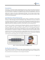
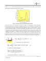
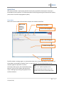
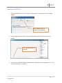
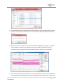
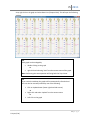
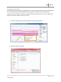
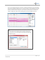
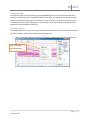
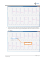
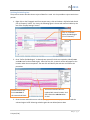
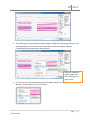
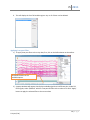
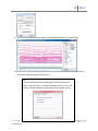
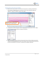
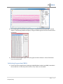
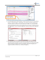
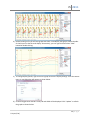
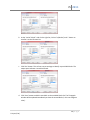
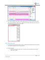
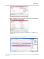
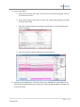
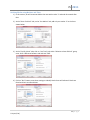
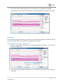
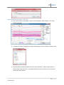
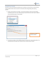
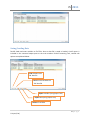
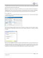
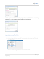
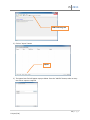
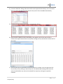
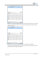
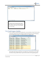
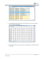
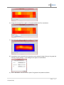
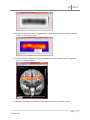
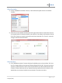
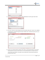
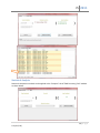
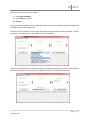
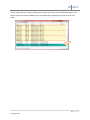
fnirSoft
A Quick Start Guide
12/27/2011
Drexel University
Hasan Ayaz
fS 2011
Please refer to fnirSoft in your publications with the following:
Ayaz, H. (2010). “Functional Near Infrared Spectroscopy based
Brain Computer Interface”. PhD Thesis, Drexel University,
Philadelphia, PA.
Disclaimer
THIS SOFTWARE IS PROVIDED ''AS IS'' AND ANY EXPRESS OR IMPLIED WARRANTIES, INCLUDING,
BUT NOT LIMITED TO, THE IMPLIED WARRANTIES OF MERCHANTABILITY AND FITNESS FOR A
PARTICULAR PURPOSE ARE DISCLAIMED. IN NO EVENT SHALL THE AUTHORS OR COPYRIGHT
HOLDERS BE LIABLE FOR ANY DIRECT, INDIRECT, INCIDENTAL, SPECIAL, EXEMPLARY, OR
CONSEQUENTIAL DAMAGES (INCLUDING, BUT NOT LIMITED TO, PROCUREMENT OF SUBSTITUTE
GOODS OR SERVICES; LOSS OF USE, DATA, OR PROFITS; OR BUSINESS INTERRUPTION) HOWEVER
CAUSED AND ON ANY THEORY OF LIABILITY, WHETHER IN CONTRACT, STRICT LIABILITY, OR TORT
(INCLUDING NEGLIGENCE OR OTHERWISE) ARISING IN ANY WAY OUT OF THE USE OF THIS
SOFTWARE, EVEN IF ADVISED OF THE POSSIBILITY OF SUCH DAMAGE.
2|Page
H. Ayaz (1.0e)
fS 2011
Table of Contents
Introduction .................................................................................................................................................. 5
Functional Near Infrared Spectroscopy .................................................................................................... 5
Modified Beer Lambert Law ..................................................................................................................... 5
Quick Start..................................................................................................................................................... 8
Overview ................................................................................................................................................... 8
Loading raw fNIR files ............................................................................................................................... 9
Loading marker files ................................................................................................................................ 12
Preprocessing .......................................................................................................................................... 14
Rejecting Channels .............................................................................................................................. 14
Defining Exclude Regions .................................................................................................................... 17
Applying Low-pass Filter ..................................................................................................................... 19
Applying Motion Artifact Rejection (SMAR) ....................................................................................... 21
Calculating Oxygenation (MBLL) ............................................................................................................. 22
Block Analysis .......................................................................................................................................... 25
Defining Blocks .................................................................................................................................... 26
Defining Blocks using Markers ............................................................................................................ 27
Define Blocks using Time .................................................................................................................... 30
Defining Blocks using Markers and Time ............................................................................................ 33
Using blocks ........................................................................................................................................ 34
Exporting Blocks directly to a Matlab™ File ........................................................................................ 34
Exporting Blocks directly to a Text File ............................................................................................... 35
Saving Blocks as Variables ................................................................................................................... 36
Saving/Loading Data ............................................................................................................................... 37
Exporting Data ........................................................................................................................................ 38
Importing Data from Text Files ............................................................................................................... 39
View/Graph/Compare Variables ................................................................................................................. 43
Visually comparing variables................................................................................................................... 46
Topograph and Visualization .................................................................................................................. 51
3|Page
H. Ayaz (1.0e)
fS 2011
Processing Tool ........................................................................................................................................... 56
Select Variables ....................................................................................................................................... 57
Select Actions .......................................................................................................................................... 57
Statistical Analysis ................................................................................................................................... 59
References .................................................................................................................................................. 62
4|Page
H. Ayaz (1.0e)
fS 2011
Introduction
fnirSoft (fS) is a stand-alone software package designed to process, analyze and visualize functional near
infrared (fNIR) spectroscopy signals through a graphical user interface and/or scripting (for automation).
This section provides an introduction to the fNIR technology and discusses Modified Beer Lambert Law
(MBLL) that is integral to the analysis of fNIR spectroscopy signals. The next chapter provides step-bystep guide for using fS. For information about fnirSoft programming and command line options, please
refer to fnirSoft Scripting Manual.
Functional Near Infrared Spectroscopy
fNIR is an optical brain monitoring technology that monitors changes in hemodynamic response within
cortex [1-3] . fNIR technology uses specific wavelengths of light, introduced at the scalp, to enable the
noninvasive measurement of changes in the relative ratios of deoxygenated hemoglobin (deoxy-Hb) and
oxygenated hemoglobin (oxy-Hb) in the capillary beds during brain activity. This technology allows the
design of portable, safe, affordable, noninvasive, and minimally intrusive monitoring systems.
Our focus here is analysis of continuous-wave fNIR signals collected by the Drexel fNIR system. The
system is composed of two parts: a hardware box and a flexible sensor pad that is placed over the
forehead of subjects. With a fixed source-detector separation of 2.5 cm, this configuration generates a
total of 16 measurement locations (voxels) per wavelength. The sensor pad as shown in Figure 1 below.
The hardware box is connected to a computer via a standard universal serial bus (USB) cable for data
acquisition and control via Cognitive Optical Brain Imaging (COBI) Studio [2] that was also developed at
Drexel University. The system records two wavelengths and dark current for each 16 voxels, totaling 48
measurements for each sampling period. The sampling rate of the system is 2Hz.
Figure 1. Latest generation fNIR Sensor (fNIRDevices.com)
Modified Beer Lambert Law
For a medium that contains chromophores (light absorbing molecules) and no scattering, the BeerLambert Law states that the ratio of incident and response (detected) light intensity is proportional to
the concentration of the chromophore in the unit length of the medium:
5|Page
H. Ayaz (1.0e)
fS 2011
I
log( 0 )   cL
I
(1)
where I 0 is incident light intensity and I is the detected light intensity. c is the concentration of the
chromophore. L is the distance from where light enters the tissue to where it leaves the tissue. Finally,
 is the absorption coefficient of the chromophore.
However, tissue is a highly scattering medium and L does not reflect the true path length. Scattering
significantly prolongs the path length of light. To account for that, the modified Beer-Lambert law can be
used:
I
log( 0 )   cLB  G
I
(2)
where I 0 , I , c ,  and L are the same as in the previous equation. B is an experimentally determined
correction factor for L. G is constant attenuation factor related to optical properties and geometry of
the tissue. If measurements are made of the changes in attenuation, the Modified Beer Lambert Law
can be rearranged as follows:
c 
where
OD
 LB
(3)
OD  log(
I0
)
I
(4)
To calculate changes in the concentrations of the chromophores, we need to compare two
measurements: one from the subject in a “rest” state as a baseline, and one during the presentation of
the stimulus or “test” condition. This comparison can be expressed as follows:
OD  log(
I0
I
)  log( 0 )
I test
I rest
 log( I rest )  log( I test )
I
 log( rest )
I test
(5)
6|Page
H. Ayaz (1.0e)
fS 2011
where
I rest is the measured reflected light intensity in the baseline condition, and I test is the reflected
light intensity during the presentation of the stimulus.
Figure 2 Absorption factors of 3 main chromophores in tissue
Brain tissues have three significant chromophores: water, oxy-hemoglobin (oxy-Hb) and deoxyhemoglobin (deoxy-Hb). In functional brain imaging applications, the main interest is to monitor oxy-Hb
and deoxy-Hb concentration changes. Within the 700-900nm range, or “optical window“, tissue is
relatively transparent because all significant chromophore absorption factors are low. The dominant
chromophores in the optical window are oxy-Hb and deoxy-Hb, and their concentration changes can be
calculated using Equation 3. Absorption factors of the three main chromophores with respect to
wavelength are given in Figure 2. Within the optical window, there is an isosbestic point where the
absorption spectra of oxy-Hb and deoxy-Hb cross. Measurements by choosing two wavelengths, one
below and one above this isosbestic point, could reveal the individual effects of oxy-Hb and deoxy-Hb.
(6)
(7)
7|Page
H. Ayaz (1.0e)
fS 2011
Quick Start
This section provides a step-by-step tutorial for basic tasks required for data analysis. Each step is
illustrated by screen captures. For information about fnirSoft programming and command line options,
please refer to fnirSoft Scripting Manual (2011).
Overview
Below is the main window of fnirSoft with common user elements identified.
Open a new
editor to
view/edit
scripts
View/Process Variables
Create a new Topograph
Create a new Timegraph
Command output pane
Command prompt
fnirSoft includes a scripting engine, so commands written to the “command prompt” at the bottom of
the window are executed by pressing “Enter” on your keyboard. The command prompt can also
evaluate algebraic expressions. For more
TIP
information about syntax, see the fnirSoft Scripting
Type “2 +3” (without quotes) at the
Manual. The rest of this chapter will detail basic
command prompt and press enter. You
steps in fNIR signal processing with graphical user
should see the result 5 at the output pane.
interface elements.
8|Page
H. Ayaz (1.0e)
fS 2011
Loading raw fNIR files
1. Click on the ‘fNIR Data Tool’ at the toolbar of main window. This will open a new Timegraph
window.
Click “fNIR Data Tool” to
create a new Timegraph.
2. In the Timegraph window, click on the ‘Load Data’ Button at the lower left corner of the
window.
Click ‘Load Data’ button to
select file
3. A file selection window will appear. COBI data files in three formats are recognized (*.nir, *.xls
and*.txt). Select the *.nir to open.
9|Page
H. Ayaz (1.0e)
fS 2011
4. If the selected file is part of an experiment saved by COBI, it might be accompanied by a marker
file for time and event information. Click ‘Yes’ to also load the associated marker file with the
data file.
5. Measurements from all channels in the selected file will be displayed in the graph. If a marker
file was loaded, vertical lines corresponding to the markers will be displayed as well. The
”Properties” pane on the right hand side provides information about the current data file.
6. The data can be displayed in 2-by-8 format. This view shows data for each channel individually,
in an arrangement corresponding to the actual arrangement of the sensors used. To select this
10 | P a g e
H. Ayaz (1.0e)
fS 2011
view, right click on the graph and select Raw View (Temporal 2x8). This will open the following
window.
TIP
Each graph can be enlarged by
 double-clicking on the graph
or
 right-click and selecting ‘view’ from the context menu of the graph.
Note: Performing the same operation will bring back the 2-by-8 view.
TIP
If you resize the window, the graphs will be automatically refreshed and
this can also be manually initiated by one of the following:



Click on Update button (lower right-hand side corner)
or
Right-click and select ‘update’ from the context menu
or
Left-click on the graph
11 | P a g e
H. Ayaz (1.0e)
fS 2011
Loading marker files
Marker files that are associated with fNIR data files are automatically recognized and will be loaded with
the respective fNIR data file if using default settings. However, if data were not recorded in the
‘Experiment mode’ of COBI, marker files are not associated with the data file. In this case, ‘Load Events’
button can be used to select a marker file to load.
1. Click the ‘Load Events’ button at the bottom of the main graph window.
Click ‘Load Events’
button to select
marker file
2. Select the marker file to load.
12 | P a g e
H. Ayaz (1.0e)
fS 2011
Once a file is selected and opened, all markers are loaded and displayed on graph immediately.
Note that each fNIR file by default has the -1 (end of recording), -2 (start of baseline),-3 (end of
baseline),-4 (baseline values ready) and -5 (record button is pressed) markers and these are
shown in orange color. Other markers (in dark green) are the ones loaded from the file.
TIP
You can view a list of all loaded markers by double-clicking on the
“Current Events” item in the properties pane (right-hand side) within
“Experiment” group.
13 | P a g e
H. Ayaz (1.0e)
fS 2011
Preprocessing
The necessary steps for preprocessing may change depending on the current data and experiment
protocol. If the data is noisy, it is advised to apply a linear phase, low pass filter that attenuates high
frequency components of the signal. Furthermore, certain channels, or time periods may need to be
excluded due motion artifact, saturation or noise. fnirSoft can be used to design and apply windowbased finite impulse response (FIR) filters.
Rejecting Channels
To exclude all data from a voxel, first, go to “Raw View” window and reject or accept the selected voxel
from the “Evaluate” option at the context-menu (by right-click).
1. Right-click on the Timegraph, and select “Raw View (Temporal 2x8)” from the context menu.
Click ‘Raw View’ at
the context-menu
14 | P a g e
H. Ayaz (1.0e)
fS 2011
2. A new window will appear as shown below. In this “Raw View (Temporal 2x8)”, you can toggle
hide/view markers (by right clicking graphs and selecting Toggle Marker Display).
3. In the Raw View, right-click on the graph of the voxel you want to reject, and at the context
menu, select Evaluate > Reject.
Click on “Reject.”
4. Once rejected, the voxel graph is changed to “null” display as shown below for voxel 3:
15 | P a g e
H. Ayaz (1.0e)
fS 2011
5. To reverse this action, simply right-click on the graph of the rejected voxel and select Evaluate >
Accept from the context menu. The graph will be updated to show the voxel data instead of the
“null” display.
Click on “Accept”
16 | P a g e
H. Ayaz (1.0e)
fS 2011
Defining Exclude Regions
The previous section describes how to reject all data for a voxel. It is also possible to reject certain time
periods.
1. Right-click on the Timegraph and from context menu, click on Evaluate > Define Exclude Period
(For all Channels). NOTE: For clarity, the following figure is shown with markers hidden by the
use of the “Display Settings” button.
Click on “Evaluate >
Define Exclude Region
(For all Channels)”
2. Once “Define Exclude Region” is selected, two mouse left-clicks are required to identify start
and end times for the exclude region. After the first click, a vertical red line will appear at the
location under the mouse pointer. The next click will identify the end time and finalize the
procedure.
The first vertical red
line is start time of
this new exclude block
The second vertical red line is
updated with mouse location. And
will indicate the end time when
clicked
3. Once the start and end times are selected, the graph is immediately updated to exclude the
selected region. NOTE: Selecting exclude regions do not delete/remove data.
17 | P a g e
H. Ayaz (1.0e)
fS 2011
4. All exclude regions can be deleted by right-clicking the Timegraph and selecting Evaluate > Clear
All Exclude Regions in the context menu. Selecting this is option will update the graph
immediately and all exclude regions will be deleted.
Select this to delete all
exclude regions and
return the graph to its
original state.
5. You can view a list of all defined exclude blocks by right-clicking the Timegraph and selecting
Manage > Exclude Regions in the context menu.
18 | P a g e
H. Ayaz (1.0e)
fS 2011
6. This will display the list of all exclude regions. Any or all of them can be deleted.
Applying Low-pass Filter
1) To apply a low-pass filter to the noisy data, first, click on the Refine button at the toolbar.
Click Refine button to see
available options
2) A popup windows will appear that displays available algorithms in different tabs. Under FIR
Filtering tab, select “$default” which is a low pass FIR filter with an order of 20. Click “Apply”
button to apply the selected filter to the current data.
19 | P a g e
H. Ayaz (1.0e)
fS 2011
3) The filter will be applied and the graph will be updated immediately, as shown below:
4) Filtered data do not replace original (unfiltered) data. Both are accessible with functions to be
exported or used for oxygenation calculation.
TIP
To return to viewing unfiltered data, right-click on the graph and
select “Display Settings”. In the pop-up dialog, under the “Filter” tab,
select the “Show Unfiltered” option and click the “Update” button.
20 | P a g e
H. Ayaz (1.0e)
fS 2011
Applying Motion Artifact Rejection (SMAR)
1) Motion artifacts and saturation can be detected automatically by a Sliding-window Motion
Artifact Rejection (SMAR) algorithm. See Ayaz et. al. [4] for more information about the
algorithm. To apply, click “Refine” button at the toolbar.
Click Refine button to apply sliding
window motion artifact rejection
2) A configuration window will appear to allow changing algorithm parameters. Click the “Apply”
button to accept current parameters and apply the algorithm.
3) Segments identified as motion artifacts and saturated channels will be excluded automatically.
Compare the following graph with the one in step 1 above. Also, see the command output pane
(at the main window) for a brief report. The graph will be updated immediately.
21 | P a g e
H. Ayaz (1.0e)
fS 2011
4) All exclude regions can be seen by right-clicking on the graph and selecting Manage > Exclude
Regions. The following window will appear, listing all exclude regions with start and end times in
parenthesis.
5) To clear all exclude regions, right-click on the graph and select Evaluate > Clear All Exclusions
from the context menu.
Calculating Oxygenation (MBLL)
1) fnirSoft calculates oxygenation by applying the Modified Beer Lambert Law (MBLL) described in
the introduction. To start the process, click the “Oxy” button on the toolbar.
22 | P a g e
H. Ayaz (1.0e)
fS 2011
Click ‘Oxy’ button to
calculate oxygenation
data
2) The following parameter window will appear. Under the General tab, you can select different
baselines, and specify filtered or unfiltered data. The Coefficients tab allows modifying the
absorption spectrum coefficients of oxy-Hb and deoxy-Hb of MBLL. The “Use filtered data”
option will be disabled if no filter has been applied to the current data. The default baseline is
the “COBI Baseline”. Click the “Calculate Oxygenation” button to accept current settings and
continue.
3) Once oxygenation data is calculated, a new window will appear that displays 16 voxels
separately as follows. By default, all markers and exclude regions are transferred. The graphs
displays Hb (deoxy-hemoglobin), HbO2 (oxy-hemoglobin), HbT (total hemoglobin) and
oxygenation (difference between oxy- and deoxy-hemoglobin).
23 | P a g e
H. Ayaz (1.0e)
fS 2011
4) Double-clicking on any of the voxel graphs will zoom in and display that graph. Another doubleclick will return to the 16-voxel display. Alternatively, you can right-click and select “View”
instead of double-clicking.
5) To change display options, right click on the graph and select “Display Settings” from the context
menu. A new dialog box will appear as shown below.
6) Uncheck Oxygenation and HbT so only Hb and HbO2 will be displayed. Click “Update” to refresh
the graphs as shown below.
24 | P a g e
H. Ayaz (1.0e)
fS 2011
7) You can apply various filters using Filter tool available on the toolbar. To save and/or export
data and apply block analysis, see the next section.
Block Analysis
Here, a “block” refers to an epoch/segment of data, defined by a start time and end time and contains
all channels (48 for raw data blocks and 16 for oxygenation data blocks).
Block analysis is ideal for event related analysis. For example, blocks before and after events can be
compared across trials and within subjects. The remainder of this section describes various ways to
define blocks. All of these apply to the “Define Blocks” tool, available in both the “raw” and
“oxygenation” windows. Once blocks are defined, they can be exported, saved and further processed.
1) The following data file and event file are loaded for the reminder of the section:
2) Available events are -5 (Recording Started), 1, 1, 2, 2, 3, and -1 (Device Stopped).
25 | P a g e
H. Ayaz (1.0e)
fS 2011
Defining Blocks
The “Define Blocks” tool is available in both the “raw” and “oxy” view windows by clicking the “Define
Blocks” button on the toolbar. The following window will appear, allowing you to define blocks
separately by using marker(s), absolute time or relative time.
There are 5 steps in creating blocks. Multiple blocks or a single block can be created with each run. The
steps are as follows; details of each step are provided in the next sections.
1)
2)
3)
4)
5)
Define “Start of a block”
Define “End of a block”
Run current settings
See the report at the output pane.
Save the new found blocks to current list
1
3
TIP
To see current list of
blocks, click manage
button. A new window
with list of blocks will
appear.
2
4
5
26 | P a g e
H. Ayaz (1.0e)
fS 2011
Defining Blocks using Markers
1) In this section, we will create two blocks: one between the two ‘1’ markers, and another
between the last ‘2’ marker and the ‘3’ marker.
2) Both “Start of a block” and “End of a block” sections has two lists: one empty and the other one
with all available marker types as source. Transfer any type and number of markers from these
lists on the right to the left to create a pattern that specifies start and end of blocks.
3) For the first block:
a. On the “Start of a block” side: On the right list, click to select the ‘1 (Marker)’ item and
then the ‘<’ button to transfer it to the left-most list.
TIP
Double-clicking on list
items transfer them to
the next list.
b. On the “End of a block” side: On the right list, click on the ‘1 (Marker)’ and then the ‘<’
button to transfer it to the left-most list. . The window should appear as follows:
c. Now that we have identified the start and end of the block, click the ‘Run’ button at the
bottom of the window. fnirSoft will search the data for all blocks that can be defined as
beginning and ending with a “1” marker. All found blocks will be listed in the text box
just above the buttons, as indicated below:
27 | P a g e
H. Ayaz (1.0e)
fS 2011
Indicates how many
blocks have been found
with the current settings.
Start and end times for
each found block are
within parentheses.
d. Click the “Save” button at the bottom of the window to save the block. On the
timegraph window, the block will be shown by a colored (in this case blue) bar drawn
between the start and end times, just below the X axis.
4) For the second block:
a. At the “Start of a block” side: On the right list, click on ‘2 (Marker)’ and ‘<’ button to
transfer it to the left-most list. Click the ‘<’ button again to add another ‘2 (Marker)’.
This indicates our block start with a successive ‘2’ markers.
TIP
You can apply labels (that are simply strings) to tag blocks you have created.
To do that, add any string (separate by comma for multiple labels) to “Apply following label” field.
If you use # within the label, block index numbers will be added to the label. For example, with
“sample#” temple, and if 3 blocks are created, they will have “sample0”, “sample1” and
“sample2”.
28 | P a g e
H. Ayaz (1.0e)
fS 2011
b. At the “end of a block” side: On the right list, click on ‘3 (Marker)’ and ‘<’ button to
transfer it to the left-most list.
c. Click ‘Run’ button. This will use current settings to identify any available blocks. The
output pane indicates 1 new block found.
d. Click ‘Save’ button to add this new block to the available blocks list. The Timegraph
window will be updated immediately to show the second block (in this case magenta
color).
29 | P a g e
H. Ayaz (1.0e)
fS 2011
5) All currently available blocks can be listed by right clicking on the graph, and from the contextmenu, selecting Manage > Blocks. Here, it displays the two blocks created. Any one of them can
be deleted and the whole list can be re-sorted.
Define Blocks using Time
1) In this section, we will create two blocks, the first one with start and end times as 30 sec and 70
sec. And the second block, with 90 sec and 200 sec.
2) For the first block:
a. At the “start of a block” side: click on “Use Time” Tab. Under fixed time, enter 30 for
‘block starts at’ field.
30 | P a g e
H. Ayaz (1.0e)
fS 2011
b. At the “End of block” side, click on “Use Time” tab and enter 70 at the within fixed time
group, for “block ends at” as shown below.
c. Click “Run” button to apply these settings to identify blocks. Pane will indicate that it
found 1 block.
d. Click on “Save” button to add this block to current block list. The timegraph window will
be updated immediately to visualize the block.
31 | P a g e
H. Ayaz (1.0e)
fS 2011
3) For the second block:
a. At the “start of a block” side: under “Use Time” Tab. Under fixed time group, enter 90
for ‘block starts at’ field.
b. At the “end of a block” side: under “Use Time” Tab. Under fixed time group, enter 200
for ‘block ends at’ field.
c. Click “Run” button to apply these settings to identify blocks. Pane will indicate that it
found 1 new block.
d. Click “Save” button to add this new block to current block list.
4) All blocks can be cleared by the “Clear All” button at the “Define Blocks” tool window. Or, by
right-clicking the graph and from the context menu, selecting, Manage>Blocks and “Delete All”
at the new window.
32 | P a g e
H. Ayaz (1.0e)
fS 2011
Defining Blocks using Markers and Time
1) In this section, we will create two blocks that start with marker ‘2’ and ends 10 seconds after
that.
2) At the “Start of a block” side, at the “Use Marker” tab, add only one marker ‘2’ to the list as
shown below.
3) At the “End of a block” side, click on “Use Time” tab, within “Relative to Start of block” group,
enter 10 for ‘difference between end and start’ field.
4) Click on “Run” button to use these settings to identify blocks. Pane will indicate 2 blocks are
found and their start & end times.
33 | P a g e
H. Ayaz (1.0e)
fS 2011
5) Click “Save” button to add these blocks to current blocks list. The graph will be updated
immediately to visualize them. The two blocks are have identical length and start with a marker
‘2’
Using blocks
There are different ways to use blocks. This section uses the raw data Timegraph for illustration, but the
same interface and options are available for the oxygenation view graph.
Exporting Blocks directly to a Matlab™ File
1) Click the “Save” button in the toolbar. In the menu that appears, click “Export”. Then, click “All
blocks to a Matlab™ file”.
2) A “Save As” dialog will appear, allowing you to select a file name and location for the exported
block data.
34 | P a g e
H. Ayaz (1.0e)
fS 2011
Exporting Blocks directly to a Text File
1) Click “Save” button in the toolbar. In the menu that appears, under “Export”, click “Each
block to a text file”.
2) A “Browse for Folder” dialog box will appear, allowing you to select a folder in which to save
the exported block data.
3) All blocks will be saved in separate files with names “Block#.txt”, where # represents the
block number. Each text file is in tab-separated format; the first column is the time and all
the rest are data channels.
35 | P a g e
H. Ayaz (1.0e)
fS 2011
Saving Blocks as Variables
fnirSoft has various processing and visualization tools, and data can be used if they are saved as Blocks
to be used within fnirSoft. See next section for information about saving/loading and exporting
variables.
1) Click the “Save” button on the toolbar. In the menu that appears, select the “Save all blocks
(Unfiltered)” option. This saves unfiltered (original raw) data. Note that a brief report is added in
the command output pane of main window.
Indicates that 2 blocks are
saved as variables.
2) To view these variables, click the“fNIR Processing Tool” button on the main window toolbar. The
following window will appear that indicates two pairs of data and time variables.
36 | P a g e
H. Ayaz (1.0e)
fS 2011
Saving/Loading Data
fnirSoft loads and saves variables to ‘fsd’ files. Once a data file is saved or loaded, a brief report is
included in the command output pane at the main window. fnirSoft Processing Tool, variable tab
options are explained below.
Load variables from
‘fsd’ data file
Save current variables to a
‘fsd’ data file
Export variables (Using Export Tool)
Import data (Using Import Tool)
Delete all variables
37 | P a g e
H. Ayaz (1.0e)
fS 2011
To select variables click on them, to select multiple variables, keep ctrl button (on the keyboard) pressed
and click (with mouse) on the variables listed.
Note: When saving or clearing variables, all variables in the list are saved or cleared except Timegraph or
Topograph items such as the item simply called ’g0’ in the figure below. These are objects as opposed to
data variables. They can be deleted by right-clicking and selecting Delete from the context menu.
Exporting Data
The Export Data Tool, accessible from Main window, tool top menu item, or fnirSoft Processing Tool,
variable tab, export button.
The wizard style dialog, provides 3 steps where all variables or selected ones can be saved in various
formats and styles. The first step includes selection of all variables or selection of a subset of variables
for export.
Next, one of the available file formats is selected: tab-separated text file, comma separated Excel file
and Matlab file format. Also, exported variables can be saved into separated files (one file for each
variable) or all of them into a single output file (one file for all variables). Also, a report file can be
generated. This selection saves mean and standard deviation of variables instead of all data.
38 | P a g e
H. Ayaz (1.0e)
fS 2011
At the last step, the output folder is selected by using the “select output folder” button. Also, optionally,
prefix option can be used to append a string at the beginning of each export file.
Importing Data from Text Files
1) fnirSoft can import data from any text file. To start procedure, select “Import Data Tool” under
Tools top menu item.
OR click on “fNIR Processing Tool” button at the main window toolbar.
39 | P a g e
H. Ayaz (1.0e)
fS 2011
fNIR Processing Tool
2) Click on “Import” button
Import
3) The Import Data Tool will appear empty as below. From the “Add File” button, select as many
text files to import as required.
40 | P a g e
H. Ayaz (1.0e)
fS 2011
4) From the “Add Files” dialog, select the text file to be imported. Alternatively, one or more text
files can also be drag-dropped (with mouse cursor) to this list to be added automatically.
5) A sample text file contents are shown in the Notepad as follows
6) Once the files is added to Import data dialog, it will appear in the file list and if the file is
selected, the import function with current parser settings can be previewed at the lower half of
the screen.
7) The first row of the file (see above file contents above) is not data, so we can ignore the first
row, visually, first by clicking on the left-top cell. This would enable viewing check-boxes for
each row (see below). Any row can be removed from import by clearing the respective
checkbox.
41 | P a g e
H. Ayaz (1.0e)
fS 2011
Alternatively, at the parser settings tab, enter 1 at the header group: ignore the first rows option
and hit “Preview” button to reapply current settings and view the potential output variable as
shown within the grid.
8) Click “Import” button to add this 10x16 variable to current variables. It will appear as
‘imported#’ with # to replace number. Note: If there are more than one files in the list, each file
with the same parser settings will be imported.
42 | P a g e
H. Ayaz (1.0e)
fS 2011
TIP
To quickly reach file selection step, simply
type ‘import’ at the command prompt of the
main window and hit enter. This will display
‘open file’ dialog.
View/Graph/Compare Variables
1) At the “Variables” tab of fnirSoft Processing Tool, current variables are listed. This list can be
re-sorted by clicking on any column header. fnirSoft Processing Tool can be accessed from
the main window by clicking on the “fNIR Processing Tool” toolbar button.
2) Any selected variable will be highlighted. Double click on a variable to open detail-view for
that variable. Alternatively, right click on any variable in the list and click on ‘view’. Detailview allows viewing variable contents in grid and also provides various graphing options.
43 | P a g e
H. Ayaz (1.0e)
fS 2011
3) A new window that displays all channels of the selected variable in array view will appear.
Any cell of the data can be viewed.
4) Click on “Graph View” tab to view all channels in a single graph, this is called Temporal (All in
1) type graph.
44 | P a g e
H. Ayaz (1.0e)
fS 2011
5) Type of the graph can be changed at “Graph Type” button at the toolbar.
6) Select Temporal (2 by 8) graph type from the toolbar. This view is available only for variables
with 48 columns (raw fNIR data) or 16 columns (oxy data).
45 | P a g e
H. Ayaz (1.0e)
fS 2011
7) Double click on any graph will en-large that graph. Alternatively, right-click and select “view”
from the context menu. Perform the same operation again to go back to previous view.
8) Select “Bar” from “Graph Type” at the toolbar. This will display all channels means.
Visually comparing variables
1) Select two or more variables at “Variables” tab of “fNIR Processing Tool”. To do that, keep ‘ctrl’
button (at the keyboard) and click on variables to select more variables. In the figure below, two
variables are selected.
46 | P a g e
H. Ayaz (1.0e)
fS 2011
2) Right-click on one of the selected variables and click on “View” from the context-menu.
3) Comparison of means of all channels (columns) is shown with bar graph type. Error bars are
Standard Error of the Mean (SEM) by default.
47 | P a g e
H. Ayaz (1.0e)
fS 2011
4) To edit graph properties such as range, error bar type, etc, right click on the graph and click on
“Properties” from the context-menu.
5) The properties pane will be shown on the right-hand side.
48 | P a g e
H. Ayaz (1.0e)
fS 2011
6) Change the error bars to “standard deviation” and Y-axis range maximum to 6
49 | P a g e
H. Ayaz (1.0e)
fS 2011
7) Finally, change Size field under Bar to 15 and right click on the graph and uncheck “Properties”
to close the pane.
8) This windows is resizable and also be enlarged by mouse cursor (keeping the cursor at the
border) for better view. TIP: The final graph can be copied to memory or saved as image to a file
for use in reports.
50 | P a g e
H. Ayaz (1.0e)
fS 2011
Topograph and Visualization
1) Click on Topograph button at the main window toolbar. This will create a new window and a
Topograph object that will be listed in the variables tab of the fNIR Processing Tool window.
Topograph Tool
51 | P a g e
H. Ayaz (1.0e)
fS 2011
2) By default, the Topograph object is empty. To load a variable, click on variables button at the
toolbar. All available variables will be listed in drop-down menu. If there are too many variables,
a separate window, as shown below, will appear.
3) Select a variable from the list on the left and transfer it to the selected variables list on the right
by clicking on the right arrow button.
4)
Click save button to save the list and close this window. The Topograph window will be updated
immediately.
5) Since the variable contains more than one row, temporal progression of spatial changes can be
visualized. (Similar to a video with each row being a different frame). Click play button to start.
You can drag the slider to the desired location.
52 | P a g e
H. Ayaz (1.0e)
fS 2011
6) Change the view type from regular to “Interpolated-Bordered” for visualization.
7) The graph will change immediately to reflect the changes.
8) Interpolation type, range and other properties can be changes by right-clicking on the graph and
selecting “Display Settings”. A new dialog box will appear as shown below.
9) Select “WhiteBlack” from as the color pallet. The graph will be updated as follows.
53 | P a g e
H. Ayaz (1.0e)
fS 2011
10) Change the color pallet back to “BlueRedYellow”. Right click on the graph and select “Register
Frontal” from the context-menu.
11) A new visualization window will appear that registers the data to a brain surface image. See
Ayaz et. al. (2006) for details.
12) The slider at bottom of the window is the threshold value, move the slider to 190
54 | P a g e
H. Ayaz (1.0e)
fS 2011
13) To increase the visibility, activation rendering can be changed from Transparent to Opaque for
clear image. To do this, at the top menu, select Style > Opaque
14) The current view can be saved as image from top menu, File > Save menu option.
55 | P a g e
H. Ayaz (1.0e)
fS 2011
Processing Tool
Processing tools allows a quick and visual way to apply predefined action to selected input variables.
Processing tool is available at the “Process” tab under “fNIR Processing Tool” toolbar button of the main
window. The following window will appear.
There are 3 steps needed to perform an operation:
1) Select input variable(s)
2) Select action(s) to perform
3) Execute
The outcome will be displayed at the output pane at the bottom of the window. And, new variable(s)
will be added to the current variables’ list.
3
2
1
56 | P a g e
H. Ayaz (1.0e)
fS 2011
Select Variables
1) Click on “Add/Remove Variables” button, a new window will appear that lists all available
variables.
2) Select one or more variables of interest and click ‘right-arrow’ button to move them to the list
on the right hand side. Selected variables’ name and size is also shown at the bottom of the list.
Click “Save” button to accept the selected list and close the window. The “Process” screen will
change to indicate selected variables.
Select Actions
1) Click “Add/Remove Actions” button to display all available actions as shown below. The list on
the left is categorized by processing type (Temporal/Spatial/Cell by Cell). Temporal processing
operation is performed across rows. So, for Temporal Mean, the result variable has the same
number of columns with only one row. Spatial processing is performed across columns, so for
Spatial Mean, the resultant variable has same number of rows but one column.
57 | P a g e
H. Ayaz (1.0e)
fS 2011
2) Select Temporal Processing > Averaging > Mean Within Blocks and click right arrow button.
3) Click “Save” button to accept changes and close the window. Note that “Process” tab is updated
immediately with selected settings and output variable name is automatically entered. This can
be changed if necessary.
4) Finally, click on Execute button to perform the actions on the selected variables. The outcome
will be posted at the pane as shown below. For the selected operations, temporal means of
selected two input variables are created as new variables with names process0.result0 and
process0.result1. These
58 | P a g e
H. Ayaz (1.0e)
fS 2011
Statistical Analysis
Statistical comparison methods can be applied at the “Compare” tab of “fNIR Processing Tool” window
as shown below.
59 | P a g e
H. Ayaz (1.0e)
fS 2011
Similar to Process Tool, there are 3 steps:
1) Select input variable(s)
2) Select action to perform
3) Execute
The outcome will be displayed at the output pane at the bottom of the window. And new variable(s) will
be added to the current variables list.
Selection of ‘input variables’ are same using the variable selection window interface. However, “Actions
to perform” are selected from a drop-down menu as shown below.
Once the input variable and the action to perform are selected, output variable names are automatically
filled. Also, description of selected action is added to the pane at the bottom of the screen.
60 | P a g e
H. Ayaz (1.0e)
fS 2011
Finally, clicking “Execute” button performed the analysis and creates new variables depending on the
analysis type. In this case, for ANOVA, two new variables are created: one for F and the other for p
values.
61 | P a g e
H. Ayaz (1.0e)
fS 2011
References
[1]
[2]
[3]
[4]
H. Ayaz, P. A. Shewokis, S. Bunce, K. Izzetoglu, B. Willems, and B. Onaral, "Optical brain
monitoring for operator training and mental workload assessment," Neuroimage, vol. 59, pp.
36-47, 2012.
H. Ayaz, P. A. Shewokis, A. Curtin, M. Izzetoglu, K. Izzetoglu, and B. Onaral, "Using MazeSuite and
Functional Near Infrared Spectroscopy to Study Learning in Spatial Navigation," J Vis Exp, p.
e3443, 2011.
H. Ayaz, "Functional Near Infrared Spectroscopy based Brain Computer Interface," PhD Thesis,
School of Biomedical Engineering Science & Health Systems, Drexel University, Philadelphia,
2010.
H. Ayaz, M. Izzetoglu, P. A. Shewokis, and B. Onaral, "Sliding-window Motion Artifact Rejection
for Functional Near-Infrared Spectroscopy," Conf Proc IEEE Eng Med Biol Soc, pp. 6567-70, 2010.
62 | P a g e
H. Ayaz (1.0e)