Download development of an autonomous navigation

DEVELOPMENT OF AN
AUTONOMOUS NAVIGATION TECHNOLOGY
TEST VEHICLE
By
CHAD KARL TOBLER
A THESIS PRESENTED TO THE GRADUATE SCHOOL
OF THE UNIVERSITY OF FLORIDA IN PARTIAL FULFILLMENT
OF THE REQUIREMENTS FOR THE DEGREE OF
MASTER OF SCIENCE
UNIVERSITY OF FLORIDA
2004
Copyright 2004
by
Chad Karl Tobler
This thesis is dedicated to my parents, Karl and Jan Tobler.
ACKNOWLEDGMENTS
I would like thank the many individuals that have contributed to make this project a
success, and my educational experience at UF so enjoyable. Specifically, I would like to
thank Dr. Carl Crane, III, my academic advisor and committee chair, for his continual
support and guidance during my time at the University of Florida. I would also like to
thank the other members of my supervisory committee, Dr. John Schueller and Dr.
Antonio Arroyo, for their willingness to support the project.
I also need to express my gratitude to the staff of the Air Force Research
Laboratory at Tyndall Air Force Base, for their ongoing relationship and financial
support of the CIMAR lab. This project would not have been possible without their
financial backing.
Special thanks also go to the other students in CIMAR who contributed their time
and technical expertise to the project. My time as a student in CIMAR has been a great
learning experience and is highlighted by many fond memories, largely due to the
outstanding intelligence and friendliness of the other students with whom I associated.
Finally, I would like to thank my parents, who have never wavered in their love and
support for me. They laid the foundation for everything I have achieved and become
today.
iv
TABLE OF CONTENTS
page
ACKNOWLEDGMENTS ................................................................................................. iv
LIST OF TABLES........................................................................................................... viii
LIST OF FIGURES ........................................................................................................... ix
LIST OF OBJECTS .......................................................................................................... xii
ABSTRACT..................................................................................................................... xiii
CHAPTER
1
INTRODUCTION ........................................................................................................1
1.1 Project Background ................................................................................................1
1.2 Autonomous Vehicle Development at CIMAR......................................................2
1.3 The Joint Architecture for Unmanned Systems (JAUS).........................................9
1.3.1 Overview ......................................................................................................9
1.3.2 Technical Constraints ...................................................................................9
1.3.3 System Topology........................................................................................11
1.4 Thesis Focus .........................................................................................................13
2
AUTONOMOUS VEHICLE DESIGN: A MODULAR APPROACH.....................15
2.1 Hardware Modularization.....................................................................................16
2.1.1 Hardware Modules .....................................................................................16
2.1.2 Power System Design.................................................................................17
2.1.3 Communications System Design................................................................18
2.2 JAUS Software Modularization............................................................................19
2.2.1 Communicator and Node Manager ............................................................20
2.2.1.1 Overview ..........................................................................................20
2.2.1.2 Implementation.................................................................................21
2.2.2 Primitive Driver (PD) .................................................................................22
2.2.2.1 Overview ..........................................................................................22
2.2.2.2 Implementation.................................................................................24
2.2.3 Velocity State Sensor and Global Pose Sensor ..........................................31
2.2.3.1 Overview ..........................................................................................31
2.2.3.2 Implementation.................................................................................32
v
2.2.4 Global Path Segment Driver.......................................................................36
2.2.4.1 Overview ..........................................................................................36
2.2.4.2 Implementation.................................................................................36
2.2.5 Subsystem Commander ..............................................................................37
2.2.5.1 Overview ..........................................................................................37
2.2.5.2 Implementation.................................................................................37
2.2.6 In Progress JAUS Experimental Components............................................38
3
ACTUATION SYSTEMS AND HARDWARE ........................................................40
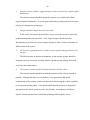
3.1 Description of a Servo System .............................................................................40
3.2 Design Process for Actuating a Vehicle Control..................................................41
3.3 Actuator Control Hardware Elements ..................................................................43
3.3.1 Servo Motors ..............................................................................................43
3.3.2 Servo Amplifiers ........................................................................................50
3.3.3 Speed Reduction, Torque Multiplication and Conversion .........................53
3.3.4 Servo Motion Controllers ...........................................................................54
3.3.5 Servo System Feedback Devices................................................................54
3.3.6 Limit and Index Switches...........................................................................56
4
ACTUATOR SUB-SYSTEMS ..................................................................................59
4.1 General Actuator System Requirements...............................................................59
4.2 Throttle Control System .......................................................................................61
4.2.1 System Parameters and Design Requirements ...........................................61
4.2.2 Design Concepts.........................................................................................61
4.2.3 System Design and Hardware Selection.....................................................63
4.2.3.1 Servo mechanism .............................................................................63
4.2.3.2 Servo motor ......................................................................................64
4.2.3.3 Servo motion controller and amplifier .............................................67
4.2.3.4 Optical encoder ................................................................................69
4.2.3.5 Limit and index switches..................................................................69
4.2.4 Satisfaction of Design Criteria ...................................................................71
4.3 Steering Control System .......................................................................................71
4.3.1 System Parameters and Design Requirements ...........................................71
4.3.2 Design Concepts.........................................................................................73
4.3.3 System Design and Hardware Selection.....................................................73
4.3.3.1 Servo mechanism .............................................................................74
4.3.3.2 Servo motor ......................................................................................75
4.3.3.3 Servo motion controller....................................................................78
4.3.3.4 Servo amplifier .................................................................................79
4.3.3.5 Optical encoder ................................................................................81
4.3.3.6 Limit and index switches..................................................................82
4.3.4 Satisfaction of Design Criteria ...................................................................83
4.4 Brake Control System...........................................................................................84
4.4.1 System Parameters and Design Requirements ...........................................84
4.4.2 Design Concepts.........................................................................................85
vi
4.4.3 Hardware Selection ....................................................................................86
4.4.3.1 Servo mechanism .............................................................................86
4.4.3.2 Smart motor......................................................................................90
4.4.3.3 Limit and index switches..................................................................94
4.4.4 Satisfaction of Design Criteria ...................................................................94
5
ACTUATOR SERVO SYSTEM ANALYSIS...........................................................96
5.1 Servo Controller Operational Theory ...................................................................96
5.2 PID Filter Tuning................................................................................................102
5.3 Actuator System Mathematical Modeling ..........................................................104
5.3.1 Integrator Mathematical Model................................................................107
5.3.2 Throttle System Model .............................................................................109
5.3.3 Steering System Model.............................................................................111
5.3.4 Brake System Model ................................................................................113
6
CONCLUSIONS AND FUTURE WORK...............................................................119
LIST OF REFERENCES.................................................................................................122
BIOGRAPHICAL SKETCH ...........................................................................................124
vii
LIST OF TABLES
page
Table
2-1
PD Hardware Components Currently Include in Tray Module ...............................28
2-2
General Component State Transition from JAUS Document .................................29
2-3
JAUS State Primitive Driver Implications ...............................................................30
2-4
Hardware Included in the Position System Module.................................................35
5-1
Throttle Actuator Motion Controller Parameter Values ........................................109
5-2
Throttle Actuator 100 Percent Step Response Attributes and Model Constants....110
5-3
Steering Actuator Motion Controller Parameter Values ........................................112
5-4
Steering System 100 Percent Step Response Attributes and Model Constants .....112
5-5
Brake Motion Controller Parameter Values...........................................................114
5-6
Brake Actuator 100 Percent Step Response Attributes and Model Constants .......116
5-7
Brake Actuator Best-Fit Second-Order Critically Damped Model Constants .......116
viii
LIST OF FIGURES
page
Figure
1-1
Navigational Test Vehicle ..........................................................................................3
1-2
The Autonomous Survey Vehicle and Metal Detecting Trailer.................................4
1-3
The Automated John Deere Excavator.......................................................................4
1-4
The AMRADS............................................................................................................5
1-5
One of Two Eliminator Vehicles ...............................................................................6
1-6
The TailGator .............................................................................................................7
1-7
Diagram of JAUS Topology ....................................................................................12
1-8
Photo of the Mule 3010 4X4 ....................................................................................14
2-1
Electronics Rack for Tray Modules .........................................................................16
2-2
JAUS Communicator and Node Manager Interaction .............................................21
2-3
Primitive Driver Command Flow.............................................................................23
2-4
Vehicle Coordinate System ......................................................................................24
2-5
Digital Input Board...................................................................................................26
2-6
Primitive Driver Hardware Tray Module.................................................................27
2-7
Current Mule Component Interface Configuration ..................................................35
3-1
Typical Servo Control System .................................................................................41
3-2
DC Motor Operational Theory .................................................................................46
3-3
Typical Torque-Speed and Power Curves for a PMDC Motor ................................49
3-4
Simplified PWM Amplifier Circuit..........................................................................51
3-5
Simple H-bridge Circuit ...........................................................................................52
ix
3-6
Encoder Output Signals and Quadrature States .......................................................56
3-7
Typical Configuration of Index and Limit Switches in a Servo System..................58
4-1
Stock Mule Throttle Control System .......................................................................62
4-2
Actuated Mule Throttle Control System ..................................................................64
4-3
Torque-Speed Curve for Throttle Servo Motor........................................................65
4-4
Torque-Speed Curve for the Gearhead Output ........................................................66
4-5
Typical LM629 Based Servo Motor Control System...............................................68
4-6
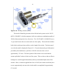
Servo Boss with Cam Tracks ...................................................................................70
4-7
Photograph of the Throttle Actuator Servo Unit ......................................................72
4-8
CAD Rendering of Steering Actuator Configuration...............................................74
4-9
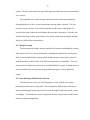
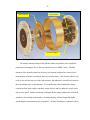
Exploded View of a Kollmorgen Servodisk Motor .................................................76
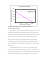
4-10 Torque-Speed Curve for U12M4H Servodisk Motor ..............................................78
4-11 AMC PWM Amplifier .............................................................................................80
4-12 Steering Limit and Index Switches ..........................................................................82
4-13 Stock Mule Steering .................................................................................................83
4-14 Modified Mule Steering ...........................................................................................84
4-15 Functional Diagram of the Brake Actuator System .................................................87
4-16 Photo of the Brake Pedal Cable Attachment Bracket ..............................................88
4-17 Brake Actuator System.............................................................................................90
4-18 The Bug Actuator......................................................................................................91
4-19 Thrust-Speed Curve for Smart Bug operated at 48 VDC.........................................92
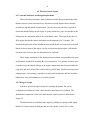
5-1
Block Diagram of Servo Systems Implemented on the Mule Actuators .................97
5-2
Trapezoidal Velocity Profile Graphs (a) Standard Profile (b) Modified Profile......98
5-3
PID Filter Block Diagram ........................................................................................99
5-4
Unit Step Response Plots .......................................................................................100
x
5-5
Step Input Produced by Throttle System Trajectory Generator .............................103
5-6
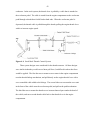
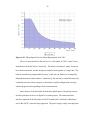
Discrete Transfer Function for Modeling Mule Actuator Systems........................109
5-7
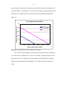
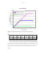
Throttle Step Response to 10, 50, and 100 Percent Step Inputs.............................110
5-8
Discrete Transfer Function Model Plotted with Actual Throttle Actuator
Response of for Step Inputs of 50 and 100 Percent Displacement ........................111
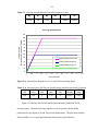
5-9
Steering Step Response to 10, 50, and 100 Percent Step Inputs ............................112
5-10 Discrete Transfer Function Model Plotted with Actual Steering Actuator
Responses to Step Inputs of 50 and 100 Percent Displacement.............................113
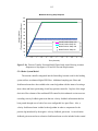
5-11 Brake Step Response to 10, 50, and 100 Percent Step Inputs................................116
5-12 Discrete Transfer Function Models Plotted with Actual Brake Actuator
Responses to Step Inputs of 50 and 100 Percent Displacement.............................118
6-1
Navigational Test Vehicle II ..................................................................................121
xi
LIST OF OBJECTS
page
Object
1
NTV2 Tele-Operation Demonstration at Tyndall Air Force Base (8.1 MB,
mule1stTeleOp.mpeg. 45 seconds) ........................................................................119
2
NTV2 Autonomous GPS Waypoint Navigation (13.2 MB,
AutonomousMule.wmv. 62 seconds).....................................................................119
xii
Abstract of Thesis Presented to the Graduate School
of the University of Florida in Partial Fulfillment of the
Requirements for the Degree of Master of Science
DEVELOPMENT OF AN AUTONOMOUS NAVIGATION
TECHNOLOGY TEST VEHICLE
By
Chad Karl Tobler
August 2004
Chair: Carl D. Crane III
Major Department: Mechanical and Aerospace Engineering
The Center for Intelligent Machines and Robotics (CIMAR) at the University of
Florida has been a leader in the field of autonomous vehicles since 1991. In order to
continue these research activities at CIMAR, a new Kawasaki Mule All-Terrain Vehicle
was chosen to be automated as a test-bed for the purpose of developing and testing
autonomous vehicle technologies. This Mule will be referred to as the Navigational Test
Vehicle II (NTV2), because it is the second generation of the Navigational Test Vehicle
(NTV) that was first automated at CIMAR in 1991. This thesis describes in detail the
design and implementation of the software and hardware systems necessary for
converting the stock Kawasaki Mule ATV into an unmanned vehicle capable of remote
control or fully autonomous operation.
As part of the automation project, servo actuators were added to the throttle, brake,
and steering systems in order to control the mobility functions of the Mule, allowing it to
operate as an autonomous vehicle. The operational theory of servo control systems is
xiii
discussed, and the throttle, brake, and steering actuator systems are described in detail. In
addition, transfer function models have been developed to predict the transient response
of each actuator control system.
A description is given of the Joint Architecture for Unmanned Systems (JAUS),
which was used as the vehicle control architecture. Because the Mule control software
has been designed according to the modular ideology of the JAUS Reference
Architecture, new software and hardware components can be readily implemented as part
of the autonomous vehicle system, allowing it to be modernized as new technologies
develop. Finally, the goals of this project were accomplished, and the Mule was
converted into a reliable development vehicle for autonomous systems technology.
xiv
CHAPTER 1
INTRODUCTION
1.1 Project Background
Unmanned robotic vehicle systems have evolved rapidly in the past two decades,
with new technologies and applications being discovered at an ever increasing pace.
Unmanned vehicle systems have been successfully developed and deployed for
agricultural, military, nuclear, and other applications that are either hazardous in nature,
or require an exacting level of precision or repeatability. Vehicle control and sensor
systems have become more advanced and reliable with the increasing availability of
smaller, more powerful computers. The modern computing capability and other
technological advancements have led to autonomous vehicles equipped with global
positioning systems capable of centimeter accuracy, detailed real-time updating terrain
maps, and obstacle avoidance systems using three-dimensional vision processing and
laser range finding sensors.
The advantages offered by unmanned vehicle systems make them well suited for
military applications. In order to develop these technologies, in 1991 the Air Force
Research Laboratory (AFRL) at Tyndall Air Force Base initiated an autonomous vehicle
program, and contracted the Center for Intelligent Machines and Robotics (CIMAR) at
the University of Florida for assistance with the project. That relationship has continued
until the present, with a continual transfer of technology between CIMAR and the AFRL
robotics research center. Research activities at CIMAR have included all aspects of
autonomous vehicle systems, such as vehicle control, path planning, positioning systems,
1
2
sensor systems, system architecture, and multiple vehicle coordination. The years of
cooperative development between CIMAR and AFRL have yielded many successful joint
projects, and produced many practical advancements in the field of autonomous vehicle
systems.
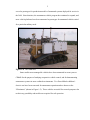
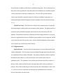
1.2 Autonomous Vehicle Development at CIMAR
The first vehicle automated by CIMAR under the direction of the AFRL was the
Navigational Test Vehicle (NTV) (see Figure 1-1). The NTV was designed using a
Kawasaki Mule 500 as the base platform. The Mule was chosen to be the first test bed
for the vehicle automation project based on its compact size, payload capacity, and
simple controls. In order to convert the Mule to the vehicle capable of autonomous
navigation, servo actuator systems were installed on the vehicle steering, throttle, brake
and shifter controls. Initially, a VME computer system was installed to command the
actuator systems and perform high-level processing necessary for navigation control and
sensory functions. Over its 10 years of service to CIMAR and the AFRL, the NTV
evolved through countless design improvements made to the actuator, sensor, and
computing systems. After a hardware or software technology was successfully developed
and tested on the NTV, it was transferred to other Air Force systems.
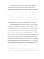
One application for the unmanned vehicle technology developed at CIMAR was for
the clean up of unexploded buried munitions. The closure of military bases by the
Department of Defense created a demand for a safe and thorough way of locating and
clearing unexploded ordnance from abandoned test ranges. Unmanned vehicle
technology offered a solution that would remove human operators from this dangerous
task, and ensure thorough coverage of the ranges by following precisely planned survey
3
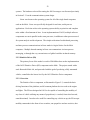
paths. In order to answer that demand, CIMAR automated a John Deere Gator that
would become the Autonomous Survey Vehicle (ASV) (shown in Figure 1-2).
Figure 1-1: Navigational Test Vehicle
The ASV was built using similar software and hardware technology that had been
developed previously on the NTV. In order to locate buried munitions, the ASV towed a
sensor package equipped with an array of magnetometers and ground penetrating radars.
The ASV autonomously navigated a carefully planned survey mission covering the
intended search field, and recorded time-stamped information from the sensors that was
post-processed to determine the exact location of possible buried munitions [Man01].
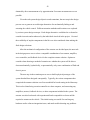
Once possible buried munitions were located, the next step in clean up effort was to
excavate and remove them. A John Deere excavator was automated for this purpose,
which could be remotely-operated a safe distance by clean up personnel (see Figure 1-3).
4
Figure 1-2: The Autonomous Survey Vehicle and Metal Detecting Trailer
Figure 1-3: The Automated John Deere Excavator
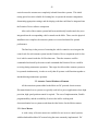
The continued technology transfer between CIMAR and the AFRL has led to other
successful autonomous vehicles. The All-Purpose Remote Transport Vehicle (ARTS)
and Autonomous Mobility Research and Development System (AMRADS) shown in
Figure 1-4 were the next-generation of autonomous vehicles that were built at AFRL
using technologies developed at CIMAR on the NTV. These vehicles have been used to
successfully demonstrate the capabilities of unmanned systems for the military, and
5
served as prototypes for production models of unmanned systems deployed for service in
the field. Since that time, the autonomous vehicle program has continued to expand, and
more vehicle platforms have been automated as prototypes for unmanned vehicles suited
for a particular military need.
Figure 1-4: The AMRADS
Some smaller more manageable vehicles have been automated in recent years at
CIMAR for the purpose of studying cooperative vehicle control, and for demonstrating
autonomous systems in more confined environments. Two PowerWheels children’s
electric cars have been converted for autonomous operation and are known as the
“Eliminators” (shown in Figure 1-5). These vehicles are useful for research purposes due
to their easy portability and smaller area required for safe operation.
6
Figure 1-5: One of Two Eliminator Vehicles
One application for multiple vehicle systems being researched with the Eliminators
is to have a formation of smaller less-intelligent child vehicles collecting and transmitting
data back to a mother vehicle with a greater level of intelligence and functional
capability. The mother vehicle would be equipped with more expensive global
positioning and guidance systems, while the small child vehicles could rely on a
positioning system relative to the mother vehicle. In this manner, the smaller vehicles
would function as a sensor array relative to the mother vehicle, and the surrounding
environment could be surveyed more efficiently.
Another small scale vehicle automated in CIMAR for technology development and
demonstration was a 50cc Suzuki Mini-Quad known as the “TailGator.” The rapid
development of this autonomous vehicle system was aided by using the Joint
Architecture for Unmanned Systems (JAUS) as described in Version 3.0 of the Reference
Architecture (RA) document. JAUS is designed to standardize the interface between
7
elements of autonomous vehicle systems. The standard message sets and component
definitions provided a framework for the integration of all systems necessary for
autonomous navigation. The TailGator was entered in the 2003 Intelligent Ground
Vehicle Competition sponsored by the Association for Unmanned Vehicle Systems
International (AUVSI) in Michigan. As a credit to the quality of systems designed in
CIMAR, TailGator won 1st place in the navigation challenge competition, which involved
following a course of GPS waypoints while simultaneously detecting and avoiding
obstacles. It also won 1st place in the vehicle tracking competition, in which it
autonomously followed another vehicle through a course using a SICK laser range
sensor.
Figure 1-6: The TailGator
Some of the greatest contributions CIMAR has made in the field of unmanned
systems technology have been in the area of modular vehicle control architectures. The
first control architecture implemented on the NTV was based on a shared memory
approach to inter-process communications. Multiple processor boards were mounted on
8
a VME backplane in order to share data and resources in real-time. The difficulties with
this system were due to the fact that a programming error in one process could overwrite
shared memory and cause an error in another process using that data, which made
debugging of the experimental systems difficult. The shared memory architecture also
presented significant difficulties when trying to upgrade hardware or software
components, or exchange them between vehicles [Sen98].
This early experience with the NTV established the need for an improved system
architecture that would reduce the difficulties encountered with, and disadvantages
inherent to the shared memory approach. In order to address this need, four design
criteria for a modular, scalable vehicle control architecture were established [Arm99].
1.
The architecture should be comprised of a set of well-defined, self-contained submodules.
2.
Software interfaces for the modules should be well defined and hardware
independent.
3.
The architecture should be scalable, so system functionality can be varied by
adding or removing sub-modules used in the system.
4.
The architecture should be a step toward the establishment of a standardized
architecture.
The guidelines for the standardized architecture listed above would result in greater
interoperability of system components between vehicles, and between alternate versions
of the same component due to the standardized interface. Several iterations of the
modular control architecture were progressively developed and tested at CIMAR in
conjunction with the AFRL. The most successful implementation was known as the
Modular Architecture eXperimental (MAX). The MAX architecture became the genesis
of a much larger scaled effort to establish a common unmanned system architecture
9
known as the JAUS working group. Much of CIMAR’s current research effort is
directed at developing and defining components for the JAUS reference architecture.
1.3 The Joint Architecture for Unmanned Systems (JAUS)
1.3.1 Overview
The Joint Architecture for Unmanned Systems (JAUS) is a collaborative effort
between military researchers, research institutions, and private industry to create a
standardized architecture for unmanned vehicles. The primary goal of creating a
standardized architecture is to reduce unmanned system life-cycle costs, by specifying an
interface standard that would allow reuse and compatibility of independently developed
system components. If built according to the JAUS standard, a particular component can
be inserted into all JAUS compliant systems, and individually upgraded or replaced as
technology advances. This is a great benefit as it allows expensive components that have
already been developed to be easily used in other vehicle systems, and for outdated or
malfunctioning components to be easily replaced. JAUS is defined to be modular and
scalable to include all the components necessary for the proposed missions and required
complexity of a system. JAUS has been designed to support the entire functional
spectrum of unmanned systems, ranging from simple remote-control functionality to fully
autonomous intelligent systems. After successful implementation and demonstrations of
JAUS controlled test vehicles, the Department of Defense has adopted JAUS as the
standard architecture for unmanned ground systems, and included it as part of the
Operational Requirements Document for the Future Combat System [Jau04].
1.3.2 Technical Constraints
Four technical constraints have been imposed on the JAUS architecture to ensure
that it satisfies the purposes for which it was created. These constraints are:
10
1.
Platform Independence
JAUS is designed to be useful for any unmanned system design based on any vehicle
platform. In order to be truly interoperable, the components specified by the JAUS
reference architecture make no assumptions about the base platform configuration or
maneuverability (i.e. Ackerman steered vs. omni-directional).
2.
Mission Isolation
The set of tasks defined for an unmanned system, which may include gathering
information about or altering the state of the environment, or both, are defined as its
missions. Mission isolation is intended to allow engineers to customize the set of
missions for an unmanned system by adding or removing components that support each
individual mission.
3.
Computer Hardware Independence
In order to capitalize on the rapid advancements in computer and sensor technology,
JAUS components should not specify a hardware standard. Computing hardware can be
selected according to the demands of a particular application. This constraint allows new
computer architectures to be used for implementing a component, which can be inserted
into an existing system to extend its life cycle.
4.
Technology Independence
There are usually multiple technical solutions to a given engineering problem, so the
architecture must not be bound to any particular technologies. Basically, this means that
no assumptions are to be made about the methods used to perform the function of a
component. For example, a JAUS position status component delivers position
information without specifying how it should be obtained (i.e. GPS, dead reckoning,
11
inertial measurement, etc.). This ensures that JAUS continues to be a viable architecture
as technology advances [Jau04].
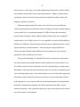
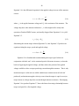
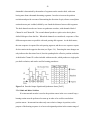
1.3.3 System Topology
JAUS is organized into a hierarchy of four levels, namely the system, subsystem,
node, and component/instance. The organization of these hierarchal elements is
illustrated in Figure 1-7. A system is a logical grouping of all subsystems that typically
would function together to gain a cooperative advantage for the complete unmanned
system. A subsystem is described as a single localized entity, usually a vehicle or robot,
hosting one or more nodes that give it give it communication, command, and control
functionality. A node is a distinct processing capability, typically the computing device,
and provides a node manager component to manage the flow of the JAUS message traffic
to the components hosted on the node. The node also provides the hardware interface
needed to support the functionality and communications of each of the software
components it hosts. The component is the lowest element of the hierarchy, and each one
provides a unique functional capability for the unmanned system. Multiple modules of
the same JAUS component can be run on a node, and are distinguished by a distinct
instance identification [Jau04].
Each component in JAUS has a strictly defined messaging interface that includes a
standard set of messages that are required to be supported by every component, and other
messages that relate to its unique functionality. It is important to note that although
JAUS defines the function and messaging structure for the component, it does not specify
how the function must be carried out. These modular system building blocks allow an
engineer to select the components required for a particular application, and add or remove
them if the mission of the vehicle system should change. Also, because JAUS
12
standardizes the communications interface of a component, an engineer can spend more
effort developing the functional performance of it, as less time is needed for
communications related issues.
Figure 1-7: Diagram of JAUS Topology [Jau04]
In essence, JAUS is a component based, message passing architecture. JAUS
defines a distinct name and identification number for every JAUS component, as well as
input and output codes and data formats specific to each component’s individual
function. Every component must also accept and execute a set of core JAUS command
codes.
Components on separate nodes communicate through the combined functions of
the Communicator and Node Manager components that are required for each node.
When a message is generated by a component, it is sent to the Node Manager, which
completes the message by attaching information pertaining to the destination component
and node. The completed JAUS message can then be passed to the Communicator,
which routes it to the indicated component residing on another node or subsystem. The
13
Communicator and Node Manager on the node receiving the message will deliver it to
the intended component, or queue the message for subsequent delivery if necessary.
1.4 Thesis Focus
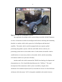
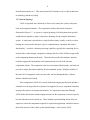
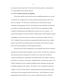
After 10 years of faithful service to CIMAR and the AFRL, the decision was made
to retire the aging Navigational Test Vehicle, and replace it with a brand new vehicle.
Due to the proven reliability and usefulness of the Kawasaki Mule platform used for the
NTV, a 2001 4x4 version of Kawasaki’s Mule was purchased to be the new CIMAR
autonomous technology development vehicle (viewable in Figure 1-8). This new Mule
will be referred to as the Navigational Test Vehicle II (NTV2), because it is the second
generation of the Navigational Test Vehicle (NTV). The control system of the new Mule
was designed based on the JAUS reference architecture, with the implementation of the
Primitive Driver (PD) intelligence component being the primary focus of this work. A
functional Primitive Driver will allow for remote control operation or autonomous
computer control of the basic driving functions of the platform. The PD accomplishes
this task by communicating with a Subsystem Commander component, and executing
servo control of all actuators that directly affect the motion of the platform.
This thesis will cover the design and development of the vehicle actuation systems
necessary to convert the new Mule into an autonomous test vehicle. After introducing
the operational theory of servo control systems, the throttle, steering, and brake actuator
systems are described in detail. Also, a description is given of the JAUS reference
architecture components that have been successfully implemented on the NTV2 to
achieve autonomous navigation.
14
Figure 1-8: Photo of the Mule 3010 4X4
CHAPTER 2
AUTONOMOUS VEHICLE DESIGN: A MODULAR APPROACH
A modular approach was taken when designing the software and hardware systems
of the Mule. The advantages of modular control architecture were discussed in Chapter 1
along with the JAUS reference architecture. Hardware modularity allows the systems
engineer to take full advantage of the benefits offered by a modular software architecture.
For example, if each functional software component was implemented in an individual
hardware unit, components could easily be added to or removed from the vehicle system.
In this way, a system could be easily reconfigured to include the components needed for
different missions. Also, components could be developed, upgraded, or replaced on an
individual basis.
There are some disadvantages to the modular approach. One obvious disadvantage
is the bulkiness of the infrastructure needed to mount, power, and link the hardware
modules. The physical capacity required for this type of set-up may not be available in
very small or weight constrained vehicles. Also, the expense of a separate computer for
each component greatly increases the cost of the overall system. For these reasons,
complete hardware modularity is usually not desirable for production model vehicles
where a high priority is placed on minimizing the size and cost of a control system.
However, in the case of a developmental platform such as the Mule, the advantages of a
modular system justify the added hardware and cost. Not all software components on the
Mule have their own hardware module. Multiple components are located in the same
hardware module either because those components function best when run
15
16
simultaneously on the same computer, or because a dedicated computer was unnecessary
or unavailable for a particular component. That flexibility is built into the JAUS
reference architecture, which makes it well suited for an “in development” system.
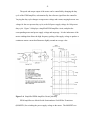
2.1 Hardware Modularization
2.1.1 Hardware Modules
The hardware standard selected as the basis for hardware modularization was the
19” rack frame common in industrial applications. This standard was adopted from the
previous NTV, where it had proven useful. Many manufactures support the 19” rack
standard, offering products designed to mount directly into the rack, or hardware modules
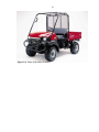
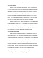
compatible with the standard. A 36” tall standard electronics rack was shock mounted to
the rear bed of the Mule as the mounting structure for the hardware modules. Slide-out
tray shelves designed for the 19” rack were selected as the basic hardware modules. The
shelves are designed to be self-contained hardware modules that can be easily removed or
inserted into the Mule system. The electronics rack filled with the tray modules is
pictured in Figure 1-1.
24-Port Ethernet Router
Obstacle Detection
Sensor Tray
Position/Velocity
Sensor Tray
Power Supply &
Distribution Tray
Figure 2-1: Electronics Rack for Tray Modules
Primitive Driver
Tray
17
In order to simplify the number and type of hardware connections that each unit
would require, standards were established for the power and communications hardware
interfaces. One 12 VDC power cord would be supplied to power each module. If other
voltages were required, the module would have to make its own conversion. Each unit
would also be allowed one RJ-45 standard Ethernet connection for the communications
system. Other permitted connections were those required to support specific component
functionality, such as signal lines from remotely mounted sensors or power lines to drive
the actuators. Amphenol military-specification connectors were used for the power lines,
and for all other connections to the trays where possible. These rugged connectors lock
together and seal out dirt and moisture, making them an excellent choice for the allterrain Mule. The connections were wired so that the “hot” side had a female connector
to reduce the risk of short-circuiting the system.
2.1.2 Power System Design
The power solution designed for the Mule electronics system relies on a 1000 Watt
gas powered generator as the primary source of electricity. The generator chosen was a
Honda EU1000, because it is equipped with inverter technology that ensures “clean”
conditioned power is delivered for use with sensitive electronics. A gas powered
generator was selected over a battery based system because it can operate over extended
periods of time with an adequate fuel supply, and there is no down-time for recharging.
The AC power output from the generator supplies a 940 Watt Uninterruptible Power
Supply (UPS) which provides battery back-up when the generator is off. While indoors,
the UPS is plugged into an extension cord from a wall outlet.
A power distribution shelf was designed as the lowest level in the electronics rack.
This shelf holds the AC to DC power converters, and splits the output to 12 available
18
power lines. A 500 Watt 12 VDC switching power supply is used to supply power to all
other tray modules. A 500 Watt 60 VDC converter supplies power for the steering motor
on an auxiliary line to the actuator control module. This exception was made to the 12
VDC supply rule because the steering motor requires a much higher voltage and enough
power that it merited a dedicated 60 VDC supply. The AC to DC power converters draw
AC power from the UPS, and output to a grid of output lines. Each power output line is
fused, and the amperage drawn from each converter is displayed by an ammeter on the
front panel of the tray. Input power to each converter is also fused and switched at the
front panel of the tray.
At the tray module, the 12 VDC power line connects to an Amphenol connector on
the back panel of the tray. The raw 12 volts is then conditioned and converted to 12 and
5 VDC by a custom built power supply board for use by the sensitive electronics. The
units are very small and are fused protected on the input and output power stages.
2.1.3 Communications System Design
In order to simplify the communication system between modules, Ethernet was
adopted as the standard interface. The communications protocol chosen for transmitting
the JAUS messages across the Ethernet lines was User Datagram Protocol (UDP). Each
unit is connected by an Ethernet patch cable to a 24 port high-speed industrial switch that
is mounted in the rack (Netgear Model FSM726). The switch routes the communication
packets to the intended recipient module according to the Internet Protocol (IP) address
assigned to each computer. The Ethernet router switch is visible at the top of the
electronics rack pictured in Figure 1-1.
In order to provide for wireless connectivity between the onboard Mule computers
and remote development systems, commercially available 802.11g Ethernet broadcasting
19
equipment was used. The IEEE 802.11g standard operates in 2.4 GHz range and
transmits data at speeds up to 55 Mbps. A D-Link wireless Ethernet access point (model
DWL-2000AP) was installed in the electronics rack and connected to the Ethernet switch.
In this manner, a wireless link could be obtained to any of the computers connected on
the Mule Ethernet network. This wireless link also allowed tele-op mobility control of
the vehicle with an Operator Control Unit laptop equipped with a wireless Ethernet card
and joystick.
2.2 JAUS Software Modularization
As specified in Chapter 1, JAUS was designed to fit the criteria of a modular,
scalable architecture. The components of JAUS are cohesive software processes that
provide some special functionality to the system. Only the functional description and
message formats are defined for each component by JAUS. The processor on which the
software is implemented, and the methods by which the information is obtained, are left
to the engineer to decide.
Hardware independence is one advantage offered by JAUS, due to the well defined
messaging interface. The only requirement JAUS places on the microprocessor used to
execute component functions is that it supports the JAUS message interface. The JAUS
message standards allow modules to exchange information without regard for how that
information was obtained or processed. This is an important feature of a modular control
architecture, because it allows different processors and different operating systems to
function together as part of the complete solution without additional interface
considerations. This gives total freedom to the systems engineer to implement each
component using any combination of processor, operating system, and programming
language deemed appropriate.
20
2.2 JAUS Components Implemented on the Mule
This section will discuss the JAUS components that have been selected as part of
the control system for the Mule. A functional description will be given for each
component (as defined by the JAUS reference architecture version 3.0), as well as details
regarding the hardware and software used for its implementation.
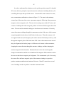
2.2.1 Communicator and Node Manager
2.2.1.1 Overview
The Communicator and Node Manager technically are separate components as
defined by JAUS. These components work closely together to handle all the message
routing in a JAUS System. Messages are routed according to the source and destination
address information contained within the message header. The sender and receiver
component addresses are indicated by a four field identifier for each in the message
header. The four fields of the address identifier are: Subsystem ID, Node ID, Component
ID, and Instance ID.
Each node in JAUS is required to have a Node Manager that is responsible for
managing the flows and controls of JAUS message traffic. The Node Manager contains
address information for all components in the system, and attaches this address to
outgoing messages generated by the components on that node. The Node Manager is the
receiver of messages delivered to that node, and depending on delivery information in the
header, delivers the message to an individual component or broadcasts it to all of them on
that node. The Node Manager also handles a priority class of messages in an exchange
between components known as a Service Connection.
The Communicator component maintains the data communication links to other
subsystems within a system. A subsystem may have a single communicator, which
21
provides a single point of entry for all JAUS messages into that subsystem. Figure 1-2 is
a graphic depicting the flow of messages between components, nodes and subsystems.
Figure 2-2: JAUS Communicator and Node Manager Interaction
2.2.1.2 Implementation
As currently implemented in the Mule subsystem, the Node Manager and
Communicator JAUS components have been combined to form a Message Routing
Service (MRS) that is included on every node. The MRS code was written by developers
at the Air Force Research Laboratory, and given to CIMAR for use and evaluation. The
code was written in C, and runs as an independent thread on processors using the Linux
operating system.
The computer hardware selected for the nodes that host the MRS threads were
single board computers. These industrial computers were chosen because they offer the
functionality of a full size computer in compact, sturdy form designed for embedded
22
systems. The hardware selected for routing the JAUS messages was discussed previously
in Section 2.3.1 on the communications system design.
Linux was chosen as the operating system for all of the single board computers
used on the Mule. Linux was specifically designed for real-time, multi-process
applications. Real-time refers to the operating systems ability to prioritize and complete
tasks within a fixed amount of time. In our implementation of JAUS, multiple software
components are run in parallel on the same processor, in addition to other processes used
for system analysis and development. The simple realization of multi-thread processing
and inter-process communications in Linux made it a logical choice for the Mule
computers. Multiple threads running in Linux can communicate via inter-process
messaging, or through the very convenient use of global variables in shared memory.
2.2.2 Primitive Driver (PD)
The primary focus of the author’s work in CIMAR has been on the implementation
of the JAUS Primitive Driver (PD) component on the Mule. The project started with a
stock Kawasaki Mule 4x4, and proceeded with the goal of producing a fully automated
vehicle, controlled at the lowest level by the JAUS Primitive Driver component.
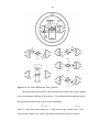
2.2.2.1 Overview
The Primitive Driver component, as illustrated in Figure 2-3, controls the basic
driving functions of the platform, and all common platform devices such as the engine
and lights. The PD was designed in JAUS to be capable of controlling the mobility of
any class of vehicle utilizing any means of propulsion (i.e. tracked, front-wheel steered,
omni-directional). In order to be useful for controlling any vehicle set-up, the PD accepts
mobility commands in the form of two wrenches, one propulsive and one resistive, that
23
define a percentile of effort in any of the three translational or three rotation degrees of
freedom for motion.
Figure 2-3: Primitive Driver Command Flow
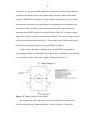
The wrenches can be resolved into three force and three moment components,
relating to the orthogonal coordinate system assigned to the assumed vehicle center of
mass, as illustrated in Figure 2-4. The convention specified by the JAUS reference
architecture is to assign the positive x axis as the forward direction of travel, the z axis
pointing downward, and the y axis as defined by a right hand coordinate system. The
propulsive wrench can be written in the form
ǒp= {fpx, fpy, fpz; mpx, mpy, mpz,}
(2-1)
in which the net propulsive translational force percentage of effort is decomposed into
components in the direction of the three coordinate axes, and the percentage of moment
effort about each axis represent the net propulsive rotational moment. The resistive
wrench is similarly defined as
ǒr= {frx, fry, frz; mrx, mry, mrz,}
(2-2)
24
which represents force and moment efforts the vehicle must produce to resist translational
or rotational movement [Arm00].
Figure 2-4: Vehicle Coordinate System
The PD translates the wrench commands into control signals for the actuators that
directly control the motion of the platform. Most platforms have limited mobility, so
only the wrench commands relating to the actuated axes of motion are applicable. For
example, a traditional front-wheel steered vehicle like the Mule can execute wrenches
commanding propulsive or restive linear effort in the x direction, or a rotational effort
about the z axis.
In the JAUS system, the PD functions in a strictly open loop manner, with platform
position/velocity control and feedback sensing responsibilities delegated to other
components. For example, a propulsive linear effort is commanded instead of a velocity,
because velocity control would require a platform velocity sensor.
2.2.2.2 Implementation
Actuator system hardware. The hardware required for the implementation of the
Primitive Driver on the Mule included: a computer for running the PD software and
communicating JAUS messages with other components, vehicle control actuator systems
25
with servo motion controllers, hardware for I/O systems, and other supporting electrical
and mechanical hardware. The mobility command wrenches for propulsive and resistive
effort in the x direction are translated by the PD into a control signal for the throttle and
brake actuator systems respectively. At the lowest level, the percentage of commanded
linear effort is scaled to the corresponding number of encoder clicks in the 0 to 100
percent position range of the actuators. Then, using position feedback from the encoder,
the servo motion controller closes the loop to seek and maintain the commanded actuator
position. Similarly, the wrenches for rotational effort about the z axis are mapped to a
steering angle controlled by the steering actuator. The design and function of the actuator
systems and their associated servo controllers are discussed in detail in Chapter 4.
Computing hardware. A single board computer (SBC) was chosen as the
processing hardware for the JAUS node that would host the PD software along with the
MRS messaging components. The SBC was ideal for this application for the reasons
discussed in Section 2.2.1.2, and because it had the interface ports needed to
communicate with the actuator motion controllers. Specifically, it had a PC/104 port and
four available serial ports, which served as the data link to the three motion controllers. It
also had two Ethernet ports built in for network communication to other nodes, and a
compact flash card slot. In order to increase the ruggedness of the computing system, a
one gigabyte compact flash memory card was used in place of a traditional hard drive for
non-volatile memory storage. This eliminated the potential failure of the rotary disk hard
drive due to the shock and vibration inherent in off highway operating conditions.
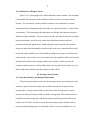
I/O hardware. In order to monitor the state of certain discrete inputs pertinent to
the control logic of the Primitive Driver, a custom digital input board was designed and
26
fabricated (shown in Figure 2-5). Three eight-bit ports are available on the ESC629
motion control board for use as digital inputs or outputs. However, in order to use this
I/O capability, the custom input board was needed in order to set the port bit signal line to
a high (+5 VDC) or low (0 VDC) state, based on the input from switch contacts. The
input board is designed to uses a supply voltage from the ESC629 board to power a line
driver chip, and provide outgoing power to the switches to be monitored. Pull down
resistors hold the input signal line for each bit low until the switch is closed, at which
point the high voltage is connected to the input channel of the line driver, which outputs
the supplied 5 VDC to signal the bit high. LEDs were also built into the circuitry to
indicate when a switch has been closed. At this point in the Mule’s development, the
steering actuator index switch, the throttle relay override switch, and the remote
RUN/PAUSE signal have been interfaced this way. It is anticipated that additional
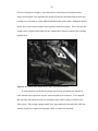
digital inputs will be added as needed.
Figure 2-5: Digital Input Board
A similar digital output board for commanding the state of discrete devices on the
Mule has been envisioned. This board would use opto-isolator chips to isolate the
discrete device circuits from the control logic electronics. This board will provide the
27
means for starting or stopping the engine, horn, lights, and other platform functional
devices.
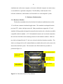
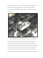
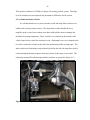
Figure 2-6 is a photograph of the Primitive Driver tray module that holds the
computer and actuator controller hardware. Table 2-1 lists the hardware currently
installed in the PD module.
Figure 2-6: Primitive Driver Hardware Tray Module
Emergency stop solution. In the event of an emergency situation, two completely
independent methods exist for a human operator to attempt to the halt the Mule. The
preferred method is to send an emergency state command to the Primitive Drive via the
wireless Ethernet link. Assuming the PD is responding and the wireless connection
exists, the PD will respond by engaging the brake at 100 percent effort, and commanding
the throttle and steering actuators to zero percent effort. The vehicle will remain stopped
in this state unit the emergency clear message is received. This software control way of
stopping an errant vehicle is referred to as a “soft-kill.” Failure of the wireless link as
28
detected by a watchdog running in the communications thread of the PD will also trigger
an Emergency state soft-kill.
Table 2-1: PD Hardware Components Currently Include in Tray Module
Component
Model Number
Vendor
Single Board Computer
NOVA 7896
ICP Electronics Inc.
Steering Motion
Controller
MVP 2001A
Micro Mo Electronics
Throttle Motion
Controller
ESC629
Real Time Devices
Steering Motor PWM
Amplifier
30A8DD
Advanced Motion
Controls
PWM Filter Card
FC15030
Advanced Motion
Controls
Digital Input Interface
Board
Custom Designed
CIMAR
DC Power Filter and
Converter
Custom Designed
CIMAR
Throttle Power Relay
KUHP-11DTT1-12
Potter & Brumfield
The other method used to stop the vehicle is through a hard-kill system that
disconnects power to the vehicle’s ignition system, which turns off the engine. In order
to ensure robust emergency kill functionality, the ignition circuit relay used for the hardkill was power by circuitry controlled by a separate wireless transmitter. A 900 MHz
Freewave radio modem was used to transmit a repeated serial string from a dedicated
laptop computer to another Freewave radio mounted on the Mule. The receive modem
outputs the serial string to a circuit that powers the ignition relay. If the emergency kill
transmitting program is exited, or the wireless link fails, the receiver circuit disconnects
power to the relay and the engine dies.
29
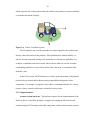
Primitive Driver states. The JAUS reference architecture defines a set of six
possible states for components, namely: Initialize, Standby, Ready, Emergency, Failure,
and Shutdown. The state of a component is queried and reported through the use of a
standard core message set. The general characteristics, transitions, and messaging relating
to these states are not discussed here, but can be referenced in Volume II (Reference
Architecture) of the JAUS Documentation [Jau04]. Suffice it to say that the control logic
of the PD has been programmed to be compliant with the JAUS specification for state
operational constraints and transitions. Table 2-2 lists the general JAUS component state
transitions. The remainder of this section will discuss specific PD implications of each
JAUS defined state.
Table 2-2: General Component State Transition Table from JAUS Document [Jau04]
State
Event
Initialize
Standby
Ready
Emergency
Failure
Shutdown
Shutdown
Standby
Resume
Shutdown
Shutdown
Shutdown
Shutdown
Shutdown
Automatic to Standby
Ready
Standby
Reset
Set
Emergency
Initialize
Initialize
Emergency
Emergency
Clear
Emergency
Standby
Initialize
Shutdown is non-recoverable
After a successful Initialization process on start-up, the PD transitions to the
Standby state. When the PD is in the Standby state, incoming wrench commands are
ignored, the throttle is set to zero percent effort, and the brake is applied at 50 percent
effort. When commanded to the Ready state, the brake is released, and the PD begins to
respond to wrench commands. An external RF remote controlled switch has been
interfaced to the PD digital input in order to signal a RUN/PAUSE command. If the
remote switch is opened, the PD puts the Mule in the Standby state until the remote
switch is closed again, when the PD resumes the Ready state. When an Emergency state
30
is signaled, the steering and throttle are sent to the zero effort positions, and the brake is
applied at 100 percent effort. This condition remains until the Emergency state is
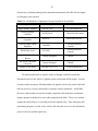
cleared. Table 2-3 summarizes the PD states.
Table 2-3: JAUS State Primitive Driver Implications
JAUS State
Primitive Driver State Implications
Initialization
x
x
x
x
x
All program control threads begin to run
Motion controller filter parameters loaded
Actuator homing sequences executed
Digital input states checked for safety logic
JAUS communications initiated
Standby
x
x
x
Wrench commands ignored
Throttle set to 0% effort
Brake set to 50% effort
Ready
x
Wrench commands executed
Emergency
x
x
x
x
Wrench commands ignored
Throttle set to 0% effort
Steering set to 0% effort
Brake set to 100% effort
Failure
x
No mobility function control
Shutdown
x
All program control threads ended
Primitive Driver software. The SBC used to process the PD software was loaded
with the Linux operating system. The code for the PD was written in the C programming
language, and structured as multiple threads to take advantage of the parallel processing
capabilities of Linux (some actuator manufacturer provided C++ libraries were also
included). The throttle, steering, and brake systems’ control logic is processed in
dedicated threads which maintain communications with the motion controllers, and
translate the mobility wrenches into position commands for the actuators. Another thread
evaluates the component state logic, and includes a watchdog sequence that signals an
31
emergency state if communications with the commanding component are lost. Also
included as part of the PD program, is a thread that handles all the JAUS message
communications. This thread and the JAUS message libraries were adopted from code
obtained from researchers at the AFRL to specifically work with their message routing
software (MRS).
A window display was created to monitor the PD using the Linux Curses library.
This display console provides information about the current state of the PD, commanded
wrench efforts, current actuator feedback positions, and identifies the component that
currently has command control. Also, if the PD is in an Emergency or Failure state, the
terminal window will display the reason why that state was activated. This visual
feedback of the PD status has been very useful for trouble-shooting and development.
2.2.3 Velocity State Sensor and Global Pose Sensor
The Velocity State Sensor and Global Pose Sensor are two different components
defined according to the JAUS Reference Architecture. In their current implementation
as part of the Mule subsystem, they receive input from the same three sensors, so it was
practical to develop them on the same node. These components, along with the Global
Path Segment Driver Component, have been developed as part of the research of another
student at CIMAR. They are briefly explained here to show how they have been
integrated into the modular control system in order to augment the Mule’s autonomous
operating capabilities.
2.2.3.1 Overview
Velocity State Sensor (VSS). The Velocity State Sensor is responsible for
determining and reporting the instantaneous velocity state of the vehicle. The velocity
state of a point in a rigid body can be described by six parameters defined in terms of a
32
fixed reference coordinate system that is coincident to that point. The six parameters are:
three linear velocity parameters in the direction of the coordinate axes, and three angular
velocity terms about each of the coordinate axes. The JAUS RA specifies that the
velocity state should be reported in terms of a reference coordinate system that is colocated and aligned with the designated vehicle coordinate system discussed in Section
2.2.2.1.
Global Pose Sensor. The Global Pose Sensor is the component that is responsible
for determining the global position and orientation of the platform. The global position is
reported in terms of latitude, longitude, and elevation as described by the WGS 84
standard. The platform orientation is defined by the Euler angle parameters <, T, and I,
related to a right-handed reference coordinate system with the x axis facing north, and the
z axis in the direction of the gravity vector. A more detailed explanation of these angles
can be found in the JAUS RA document [Jau04].
2.2.3.2 Implementation
Optical Encoder. An array of three distinct sensors is used to detect position and
velocity information. The first sensor was a two channel Dynapar optical encoder which
was installed on the drive shaft of the Mule. The rotation of the drive shaft is coupled to
the rotation of the wheels, so as the vehicle moves, the encoder emits a series of
quadrature pulses. The quadrature series indicates the direction and relative rotation of
the drive shaft, which can then be used to determine the vehicle velocity and relative
position. Due to the fact that the gear ratio between the drive shaft and drive axles is not
1:1, a series of tests were performed to determine the relationship between distance
traveled, and relative encoder counts.
33
In order for the output of the encoder to be usable by the SBC, a quadrature
decoder produced by US Digital was added. The quadrature decoder utilizes a
microprocessor to decode the quadrature signal, and provides an RS-232 serial interface
so the encoder position information can be queried by host computer. The encoder
measures the actual distance traveled by the vehicle (if it is assumed that there is no
wheel slippage), so it can be used as part of a dead reckoning position solution. Dead
reckoning is a method of calculating position based on continuously measuring the
heading and distance traveled by a vehicle. Also, the vehicle velocity can be calculated
based on the time derivative of the relative shaft rotation reported by the encoder.
Inertial measurement unit. The inertial measurement unit selected for the Mule
system was the 3DM-G produced by MicroStrain. The 3DM-G combines the sensor
output of three angular rate gyros, three orthogonal accelerometers, and three orthogonal
magnetometers in its own microprocessor designed to provide orientation information
accurate to less than 0.1 degrees. The unit is very small (approximately 3.5x 2.5 x 1 in.),
and has an update rate of 100 Hz. The 3DM-G sensor data is input to the SBC via an RS232 serial connection, where it can be used to calculate position, orientation, velocity,
and acceleration in the global reference frame. This sensor can be used to determine the
heading information necessary for a dead-reckoning position system. The 3DM-G is an
impressive sensor given its comparatively inexpensive cost (approximately $1500), but
often needs to be recalibrated due to magnetic field disturbances produced by the Mule’s
engine during vehicle operation.
GPS receiver. The third sensor implemented as part of the position and velocity
sensor suite was a Novatel Global Positioning System (GPS) receiver. The Novatel GPS
34
sensor receives telemetry data that is transmitted from a constellation of 24
geosynchronous satellites maintained by the Department of Defense. By receiving the
telemetry data from multiple satellites simultaneously, a position solution can be realized
with centimeter accuracy. The Novatel GPS receiver unit provides global position
information in the from of latitude, longitude, and altitude at a update rate of 10 Hz,
which is transmitted to the SBC through an RS-232 serial connection. The unit also
calculates current heading and velocity based on GPS position information.
Position data fusion. The major disadvantage of a pure dead reckoning approach
to a position solution is that slight inaccuracies in the sensor data accumulate over time,
causing a decay in position accuracy. The position information reported by the GPS
receiver is very accurate, but is susceptible to signal loss if direct line-of-sight with the
satellites is not maintained. In order to overcome these inadequacies, the data from all
three sensors is combined and filtered using a weighted average calculation. After
filtering, the global position, orientation and velocity information is more stable and
accurate for use by the Velocity State Sensor and Global Pose Sensor components.
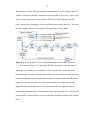
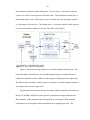
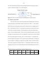
Figure 2-6 illustrates the current configuration of the sensors and the sequence of data
flow through the JAUS components.
The processing hardware used for the VSS and Global Pose Sensor was identical to
the set-up used with the PD. A single board computer equipped with a one gigabyte flash
memory card and loaded with the Linux operating system was used for interfacing the
sensors, and processing the JAUS component software. Table 2-4 lists the hardware used
in the position system module.
35
Figure 2-7: Current Mule Component Interface Configuration
Table 2-4: Hardware Included in the Position System Module
Component
Model Number
Vendor
Single Board Computer
NOVA 7896
ICP Electronics Inc.
GPS Receiver
P/N: 01016790
Quadrature Serial Adapter
AD4-B
US Digital
Inertial Measurement Unit
3DM-G
MicroStrain
Optical Encoder
HS35
DC Power Filter and
Converter
Custom Designed
Novatel
Dyanapar
CIMAR
36
2.2.4 Global Path Segment Driver
2.2.4.1 Overview
Fully autonomous operation of the Mule has been achieved by using the JAUS
Global Path Segment Driver (GPSD) as the navigational control component. The
function of this component is to perform closed loop control of the platform position and
velocity as it navigates a preplanned course of path segments defined in the global
position reference frame.
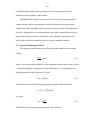
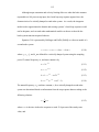
The path segments are defined by a second order polynomial that is calculated as a
function of three input points and a weighting factor. The path segments lie in the plane
formed by the control points (point coordinates given in three dimensions), with the exact
shape of the path segment depending on the location of the points and the magnitude of
the weighting factor. A more detailed explanation is available in the JAUS RA
documentation [Jau04].
The inputs to the GPSD that relate to the desired navigation course are the global
point coordinates and weights that correspond to the constituent path segments, and the
desired travel velocity. The travel velocity can be changed at any time while the vehicle
is navigating the course. In order to accomplish closed loop control of the vehicle
heading and velocity, the GPSD queries current position and velocity information from
the Global Pose Sensor and the Velocity State Sensor. The feedback data from these
sensor components allow the GPSD to stay on course at the desired speed by adjusting
the desired wrench efforts output to the Primitive Driver.
2.2.4.2 Implementation
The Global Path Segment Driver has been implemented as a software component
on the same node shared by the VSS and Global Pose Sensor. It is important to note that
37
although these three components share the same computer, in order to be JAUS
compliant, they must appear as independent components to other components not located
on that node.
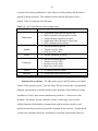
2.2.5 Subsystem Commander
2.2.5.1 Overview
The Subsystem Commander component in JAUS is the program that coordinates all
the activity within a given subsystem. This component is responsible for all mission
planning activities, high-level decision making based on input from other supporting
components, and issuing commands in order to accomplish the mission of the subsystem.
As per the JAUS RA document, the duties of the Subsystem Commander component may
be executed by a human operator, a computer, or a combination of both. The only
messaging constraints placed on the Subsystem Commander are that it needs to support
the standard core message set that is required of every component.
2.2.5.2 Implementation
At this point in the development cycle of the Mule, the Subsystem Commander has
been implemented in the form of an Operator Control Unit (OCU). The OCU is the
computer interface that enables a human operator to perform some or all of the duties of
the Subsystem Commander. The use of an OCU makes it possible to operate the Mule in
tele-op mode, where wrench commands are issued to the Primitive Driver in order to
control the mobility functions of the vehicle.
During the initial stages of the Mule PD development, a simple text-based OCU
was used to issue wrench commands to the actuator systems. This first OCU was run as a
parallel process on the same computer as the PD, and provided a text based terminal
interface for issuing JAUS commands to the PD. The OCU and PD are two distinctly
38
defined components in JAUS, so the MRS Node Manger component also had to be
running on the computer in order for the components to exchange JAUS messages. The
basic functionality of this OCU proved to be very valuable during testing and debugging
of the PD code and actuator systems.
A second, more sophisticated OCU was used later in the development cycle. This
OCU provided a graphic user interface, used joystick input to generate wrench
commands, and offered many other advanced capabilities such as video feedback display.
This OCU, also developed at the AFRL, was installed on a Dell laptop computer running
RedHat Linux version 8.0. Using the laptop’s built-in wireless Ethernet card, a wireless
connection could be established between the laptop OCU and the Mule PD node, which
allowed the Mule to operate in the tele-op mode. Testing with the Mule found the
maximum range for wireless Ethernet connection between the OCU laptop and the DLink wireless access point installed on the Mule to be approximately 500 feet with a clear
line-of-sight.
At the present time, the Subsystem Commander has only been implemented on the
Mule in the form a human operator/OCU combination. However, as more components
are added to the Mule subsystem and thereby increase its capabilities, it is anticipated that
an intelligent Subsystem Commander will be integrated as the highest level of subsystem
command control. The type of tasks that could be handled by this type of intelligent
Subsystem Commander are high-level decision making based on input from other
components, and path planning and managing operations.
2.2.6 In Progress JAUS Experimental Components
The Mule has already begun to serve its purpose as an autonomous technology test
vehicle. CIMAR is working in coordination with researchers at the AFRL to develop
39
specifications for components that have yet to be defined in the JAUS Reference
Architecture. Current student research projects include developing a smart sensor
obstacle detection component, a world model component, a dynamic path planning
component, and others. As unmanned systems technology advances, so will the demand
for new and better performing system components. In conclusion, because the Mule
subsystem has been designed according to the modular ideology of JAUS, it will continue
to serve for years to come as a test-bed for new and improved autonomous vehicle system
components.
CHAPTER 3
ACTUATION SYSTEMS AND HARDWARE
3.1 Description of a Servo System
A servo system can be described as the combination of components functioning
together to perform closed loop control of position or velocity of an actuated assembly.
A servo control loop controls the position and/or velocity along one axis of freedom of
the assembly, so multiple servo loops are need if multi-axis position control is desired.
Typically, the desired position or velocity (depending on which control mode is chosen)
is output from a host computer, or other external reference source, into a programmable
motion controller. The motion controller determines the error between the commanded
and actual position, then uses this position error to calculate the output signal based on
pre-programmed velocity, acceleration, and PID filter parameters. The control signal
generated by the motion controller is then routed to a servo amplifier, which amplifies the
control signal to the voltage and amperage levels necessary to drive a DC motor. The
motor is usually coupled to some form of gear reduction and then to the assembly that is
being position controlled. One or multiple feedback devices connected to the motor or
assembly return actual position and velocity feedback to the motion controller, which
recalculates the position error and issues new control signal based on the updated position
information. Once the desired position is reached, the closed loop servo system will
attempt hold that position, even if the load on the actuator changes. Figure 3-1 illustrates
a simplified servo control system block diagram.
40
41
Figure 3-1: Typical Servo Control System
3.2 Design Process for Actuating a Vehicle Control
This section describes the general approach used for designing and implementing
servo actuator systems on the vehicle steering, throttle, and brake controls. Sub-system
design constraints and decisions specific to the steering, throttle, and brake control
actuators are detailed in individual sections of Chapter Four.
The first task in the actuator design process was to outline the general design
specifications and functional requirements that would be applicable to all the vehicle
actuator systems. These included standards for serviceability, reliability, and aesthetics.
Also included in these are universal functional requirements, such as the actuator must be
simple to transition between manual and autonomous operational modes.
After the general design criteria for the Mule systems were outlined, the automation
process for the Mule continued by defining the design parameters and restrictions for
each of the vehicle control sub-systems. This involved measuring the physical
requirements for engaging each vehicle control mechanism. Design requirements
included the required actuation force or torque, required actuation time, dimensional
constraints, and other factors influencing the selection of an actuator. These metrics were
42
obtained by direct measurement or by approximation if accurate measurement was not
possible.
Given the sub-system design objectives and constraints, the next step in the design
process was to generate several design alternatives for mechanically linking to and
actuating the vehicle control. Different actuation methods and locations were explored
by various system design concepts. Each design alternative would then be evaluated to
consider its merits and weaknesses by the individuals involved in the project. Cost and
the availability of surplus components in the lab were also considered when making the
final design selections.
After the mechanical configuration of the actuator was decided upon, the next task
in the design process was to select a compatible combination of servomotor, amplifier,
servo controller, and feedback device for the complete actuator solution. Options to
consider when choosing a method of actuation are whether the system will be driven
electromechanically, hydraulically, or pneumatically or by some combination of fluid and
electric power.
The next step in the actuation process was to build a physical prototype of the
system that had been designed conceptually. Typically, the various components that
comprised the actuator solution were first assembled for bench-testing in the laboratory.
This involved interfacing a motion controller to a host computer, and connecting any
amplifiers, motors, feedback devices, or other components included in the system. The
actuator was also load tested with experimental loads comparable to what would be
required to actuate on the vehicle. This initial testing was useful for resolving any
hardware and/or software integration issues, and made trouble shooting any problems
43
easier because the actuator was completely isolated from other systems. This initial
testing period was also valuable for learning how to operate the actuator components,
determining appropriate settings, and developing code that could later be integrated into
the Primitive Driver software component.
After each of the actuator systems had been satisfactorily bench-tested, they were
integrated into the corresponding vehicle controls on the Mule. Then, once the physical
installation was complete, the actuator systems were tested and tuned for optimal
performance.
The final step in the process of actuating the vehicle controls was to integrate the
control code for each actuator system into the Primitive Driver component used for lowlevel vehicle control under the JAUS architecture. Then the actuators could be
commanded and tested by the same wrench commands the Primitive Driver would be
receiving during autonomous operation. This stage also allowed the actuator systems to
be operated simultaneously, in order to verify that all systems could function together as
intended during autonomous operation.
3.3 Actuator Control Hardware Elements
All the actuation systems added to the Mule use DC powered electric motors.
Electromechanical servo systems are typically used in low power applications where high
precision, high speed position control is required. The ease of implementation, flexible
programmability, and the availability of tools in the lab for working with
electromechanical servo systems made them the ideal choice for the Mule actuators.
3.3.1 Servo Motors
A wide variety of electric motors are available for use in servo control systems,
with brushed and brushless DC motors being the most commonly implemented. DC
44
motors come in a wide range of sizes and configurations, and must be selected to match
to performance requirements of the system being designed. Things to consider when
choosing an electric motor are the torque and speed capabilities, and the voltage and
amperage required for operation.
Permanent magnet brushed DC motors were used in the steering and throttle
control actuator designs on the Mule due to their availability and ease of implementing in
a servo control loop. For permanent magnet DC (PMDC) motors, the relationship
between torque and speed is linear, making controller design easier due to simplified
system analysis. Also, PMDC motors are very compatible with pulse width modulation
(PWM) servo amplifiers, which typically provide the power amplification of the control
signal produced by a motion controller. These advantages, along with their costeffectiveness and reliability, make PMDC motors the popular choice for low power
applications where cleanliness is not critical.
The typical disadvantages of a brushed DC motor are maintenance requirements
due to the wearing of the graphite brushes used to transmit power to the armature coils.
The brushes need to be replaced when they wear to the point that they no longer contact
the armature, release dust into the environment as they wear, and have a potential to arch
when switching contact points. These disadvantages were not critical in their application
to the Mule systems, because the relatively low hours of use mean the brushes will not
need replacing for a very long time, and because the small amounts of dust generated by
the brushes is insignificant compared to the dust encountered in the Mule’s typical
outdoor environment. Also, possible arching is not a safety concern because the Mule is
not used in explosive environments.
45
In order to understand the techniques used to perform position control of a brushed
DC motor, the basic principles of operation must be understood, including the theory for
controlling the torque and speed of the motor. A brushed DC motor consists of a stator,
rotor, commentator, and brushes as shown in Figure 3-2. The stator is the stationary
external part of the motor that creates a permanent magnetic field using either permanent
magnets or electro-magnetic coils. The rotor is the rotating center of the DC motor, and
consists of windings that when energized, produce an electrical field to oppose that of the
stator. The rotor and its attached windings are also known as the armature. Electricity
enters the armature windings through the commutator section of the rotor, which contacts
energized graphite brushes that are held fixed with the stator. When the armature coils
are supplied with current, the magnetic poles of the armature field attempt to line up with
the opposite magnetic poles of the fixed stator field. Just as the armature rotates toward
this pole alignment, the brushes jump to a different set of contacts on the commutator,
changing the current direction through the armature windings, and thus changing the
armature magnetic field orientation. Rotational inertia carries the rotor though the
change in commutation, and the new orientation of the magnetic fields continues to drive
the rotor toward the new magnetic pole alignment. This commutation cycle of reversing
the current flow and hence magnetic poles of the armature windings is repeated to
produce continuous unidirectional rotation of the rotor. Most DC motors have several
sets of windings in order to produce a smoother rotational motion.
46
Figure 3-2: DC Motor Operational Theory [His98]
The torque and speed of the DC motor depend on the current and voltage supplied
to the electromagnet windings of the armature. The mathematical relationship between
the output torque and current is given by the relationship
Tm k t ia
(3-1)
where Tm is the motor torque produced, k t is the motor torque constant, and ia is the
current in the armature coil. Hence, the torque produced by the motor is directly
47
proportional to the current passing through the windings of the armature. However, the
torque a motor is able to produce is limited by the amperage ratings of the electrical
components used in the motor, and by the occurrences of back electro-motive force
(emf).
Voltage is induced in a conductor when moved through a magnetic field, so when
the conductive windings of the armature spin in the field of the stator, a voltage is
induced in the windings. The induced voltage is known as back emf because it opposes
the voltage applied to armature. The back emf generated in the armature is directly
proportional to its angular velocity Za of the rotor as describe by the equation
vb
k eZ a
(3-2)
where vb is the back emf and k e is the back emf or voltage constant.
The electro-magnetic coils of the armature also act as inductors, which produce a
voltage as result of changing current, that is described by the relation
vi
La ˜
di
dt
where vi is the inductive voltage produced, La is the inductance of the coil, and
(3-3)
di
is
dt
the rate of change of the current flowing through the coil. This induced voltage is
produced by the current direction change in the windings due to commutation, and also
opposes the supply voltage applied to drive the motor. This additional inductor produced
voltage also reduces the current that can pass through the armature.
The voltage applied to the armature is equal to the sum of the back emf voltage vb ,
the inductive drop vi , and the voltage drop due to the resistance in the armature.
48
Equation 3-4 is the differential equation for the applied voltage in terms of the armature
current
va
vb Raia La ˜
di
dt
(3-4)
where va is the applied armature voltage and Ra is the resistance of the armature. The
voltage drop due to the armature inductance vi is often neglected for steady state
operation of brushed PMDC motors, and usually dropped from Equations 3-4, to yield
Equation 3-5.
va
k e Z a Ra i a
(3-5)
Substituting the current-torque relation (Equation 3-1) into Equation 3-5 produces an
equation relating the torque, speed and applied voltage.
va
k eZ a Tm ˜
Ra
kt
(3-6)
Equation 3-6 is fundamental to understanding the torque-speed relation in
conjunction with back emf. As the rotational speed of the motor increases, so does the
back emf opposing the applied voltage, and thus reduces the portion of the applied
voltage available to drive a torque producing current through the armature. That is why
maximum torque is achieved at a stalled condition (no rotation means no back emf
produced), and maximum angular velocity occurs when the torque is equal to zero (no
torque means no voltage drop from current through armature resistance). Rearranging
Equation 3-6 to produce Equation 3-7 shows the linear decreasing relationship between
torque and speed for a fixed applied voltage.
49
Tm
§k k
¨¨ e t
© Ra
§k ·
·
¸¸Z a ¨¨ t ¸¸v a
© Ra ¹
¹
(3-7)
Equation 3-7 can be plotted as a torque-speed curve illustrated in Figure 3-3.
Figure 3-3: Typical Torque-Speed and Power Curves for a PMDC Motor [His98]
In summary, it is useful to remember that in general, the torque produced by a DC
motor is proportional to the motor current, and that the motor speed is proportional to
motor voltage. The DC motor equations presented in the preceding paragraphs are useful
for selecting a motor that will satisfy the design requirements for speed and torque while
operating at the voltage and amperage levels of the available power supply. Motor
manufacturers will provide all the needed specifications, such as torque and voltage
constants ( kt and k e ), and values for motor resistance and inductance ( Ra and La ). The
motor manufacturers also generally provide torque-speed curves for various
recommended operational voltage levels, that are especially useful for selecting a motor
with suitable performance characteristics.
50
3.3.2 Servo Amplifiers
Another consideration when designing an actuation solution is how to use the
low-power output of the motion controller to drive the motor required for actuation. The
output of most motion controllers is a control level signal that cannot supply the current
or voltage required to drive a DC motor. Therefore, some method of transforming the
low-power control signal into a high-power signal capable of driving the motor is
necessary. This can be accomplished by using a servo amplifier that is designed to
accept either a digital or analog low-voltage control signal and output a higher voltage
and amperage supplied from a capable power supply to drive the motor. The control
signal produced by the motion controller is commonly an analog signal in the ± 10 VDC
range, or a low-power PWM signal, that can represent either a motor torque (current) or
velocity (voltage) demand.
Although there are various ways to amplify the control signal, pulse width
modulation amplifiers are the most popular for servo control systems due to their costeffectiveness and superior efficiency. PWM amplifiers work by rapidly switching, or
“pulsing”, a DC power supply voltage to the motor at a fixed frequency. The supply
voltage is held on for variable percentage of the repeating time period T, having the effect
of producing an average voltage at the motor that is a fraction of the supply voltage. The
percentage of the time period T that the voltage is held switched on is known as the duty
cycle. The duty cycle is defined by Equation 3-8, where ton is the time the voltage is
switched on.
duty cycle
t on
˜ 100%
T
(3-8)
51
The speed and torque output of the motor can be controlled by changing the duty
cycle of the PWM amplifier, as determined by the reference signal from the controller.
Varying the duty cycle changes average motor voltage and current, ranging between zero
voltage for the zero percent duty cycle, to the full power supply voltage for 100 percent
duty cycle. Figure 3-4 displays a simplified PWM amplifier circuit, and plots the
corresponding motor and power supply voltage and amperage. It is the inductance of the
motor windings that allows the high frequency pulsing of the supply voltage to produce a
continuous motor current that fluctuates slightly around an average value.
Figure 3-4: Simplified PWM Amplifier Circuit [Adv04a]
PWM amplifiers use Metal-Oxide-Semiconductor Field-Effect Transistors
(MOSFETs) for switching the power supply voltage to the motor. The MOSFETs are
52
switched on by a low-power PWM signal that is output from a digital motion controller,
or generated by internal circuitry based on the analog reference signal from an analog
controller. MOSFETS are ideal for use as the switches, because they are able to switch
large amounts of current at very high frequencies with minimal power dissipation, and
are relatively small. In order to operate at maximum efficiency with minimal heat
generation, the MOSFETs need to be switched fully on or fully off. An analog voltage
signal can be used to control the current through a MOSFET, but a lot of energy is wasted
as heat at states between full on and full off. This explains why a PWM control signal is
preferred over an analog voltage for driving the MOSFETs [Big03].
In order to drive the motor in both directions, the MOSFETS are arranged in a
circuit topology known as an H-bridge. In its simplest form, an H-bridge can be modeled
by four switches, a motor, and a power supply as illustrated in Figure 3-5.
Figure 3-5: Simple H-bridge Circuit [Big03]
By controlling the state of the four switches in the H-bridge, the motor can be
driven in either direction, dynamically braked, or left to freewheel. Closing only
53
switches a and d connect the supply voltage of one polarity to the motor, causing current
to flow through the motor and spin in one direction. Closing only switches b and c place
the reverses polarity on the motor, and it will spin in the opposite direction. Figure 3-5
lists possible switch states and how the motor will respond to each state. The H-bridge
circuits used in PWM amplifiers includes additional circuitry for controlling the
MOSFET switches, but the fundamental principle of operation is the same.
3.3.3 Speed Reduction, Torque Multiplication and Conversion
Generally, DC motors rotate at rates much higher than desirable for most
applications. Therefore, the speed is generally reduced to an acceptable rate and output
torque increased by some form of torque-speed conversion. Also, by reducing the shaft
speed with gears or some other torque-speed converter, a much smaller motor can be
used because the output torque has been increased. Additionally, the rotational torque
produced by the motor may need to be transformed into a linear force, depending on the
method of actuation. Therefore, in vehicle applications, the electric motors will need to
be coupled with a torque or force multiplier. A gearbox coupled to the motor is the most
common way of converting the high-speed, low-torque output to a low-speed, hightorque output. DC motors are generally available from the manufacturer with an attached
gearbox that can be selected with a gear ratio designed to produce a specified range of
rotational speed and torque. The output of the gear-head motor can then be coupled to
additional combinations of torque or force multipliers to achieve the desired amount of
force and speed in the desired direction. Other methods of increasing torque and
converting it to a linear force include belt-and-pulley sets, rack-and-pinion gears systems,
and lead screws.
54
3.3.4 Servo Motion Controllers
Another consideration when designing the actuation solutions on the Mule was
what type of servo motion controllers would be used to perform closed loop control of
each actuator system. A wide variety of motion controllers are commercially available,
with many different combinations of computational capability and features. Selection
criteria for choosing a motion controller included the hardware and communications
interfaces, required feedback signals, type of control signal produced, and additional
features offered.
Motion controllers are available in configurations supporting many different
hardware and communications standards. Motion controllers can be found in the form of
PC/104, PCI, and other card standards that insert into a port on a processor board or bus
chassis, and as standalone units that can function with or without communication from a
host computer. Communications protocols supported by the standalone type controllers
can include RS-232, RS-485, CAN, Ethernet and others. The controllers offer output in
the form of an analog voltage or as a PWM control signal. They also can be selected to
accept feedback input from most linear and rotational position feedback devices. Often,
the motion controllers come equipped with additional features such as multiple axis
control channels, programmable memory for independent operation, built in PWM
amplifiers, and analog and digital input/output ports.
3.3.5 Servo System Feedback Devices
A wide variety of position and velocity sensors are available to feedback
information necessary for the motion controller to perform closed loop motion control.
The output of the feedback sensor can be either analog or digital, and should be matched
or converted to the input capabilities of the motion controller. Among the most
55
commonly used sensors for detecting motor shaft orientation are optical encoders,
resolvers, potentiometers, and hall-effect sensors. Encoder and resolver feedback can
also be used to determine shaft velocity, as well as velocity sensing tachometers.
Optical encoders were used as the feedback sensors for determining the actuator
position of the steering, throttle, and brake systems of the Mule. An optical encoder was
also mounted on the drive shaft of Mule to provide vehicle velocity information.
Encoders are available in absolute or incremental configurations. Absolute encoders
produce a unique digital word to identify absolute shaft position, while incremental
encoders produce digital pulses as the shaft rotates that indicate relative shaft position
displacement. Incremental encoders are more commonly implemented in servo systems,
but require that a homing sequence be performed upon initialization in order to determine
absolute position. Incremental encoders were used on the Mule systems because
adequate position resolution could be obtained at an overall reduced cost than a system
implemented with absolute encoders.
Incremental shaft encoders are electro-optical devices that in simplest form are a
light source directed toward a photosensor, and separated by a disk with an incremental
slot pattern. The slotted disk is coupled to the motor shaft, so as it rotates, an electrical
pulse is emitted from the photosensor each time it senses light passing through a slot.
The number of pulses generated indicates relative shaft position, while the number of
pulses counted per unit-time indicates shaft velocity.
Optical encoders typically use an LED as the photo source and a phototransistor as
the photo detecting sensor. The disk is usually made of glass or metal, and is
incremented with alternating opaque and transparent segments. The position resolution
56
obtainable is determined by the number of segments on the encoder disk, with some
having more than a thousand alternating segments. In order to increase the position
resolution and provide a means of determining the direction of spin, often a second photo
emitter-detector pair is added, shifted by one fourth the distance between disk segments.
The dual channel encoders are known as quadrature encoders, with channels labeled
Channel A and Channel B. The second channel produces a pulse series that is phase
shifted 90 degrees from the first. When both channels are considered, a sequence of four
different output states are possible with each passing disk segment. As the disk rotates,
the state sequence is repeated for each passing segment, and the reverse sequence repeats
for the rotation in the opposite direction (see Figure 3-6). Detecting the state changes not
only indicates the direction of travel, but also quadruples the effective position resolution.
A third index Channel Z is often included with an encoder, which produces a single pulse
per shaft revolution, and can be used for homing procedures.
Figure 3-6: Encoder Output Signals and Quadrature States [Fre95]
3.3.6 Limit and Index Switches
If an incremental encoder is used as the position sensor in the servo control loop, a
homing routine must be performed on start up in order to be useful as an absolute
position sensor. Incremental encoders only sense relative changes in position, so the
purpose of the homing sequence is to locate a designated position in the actuator range of
57
motion as the “home” position. Once the home position is located and set in the
controller, absolute position can be identified as the distance relative to the home
position.
A typical homing routine begins by commanding the actuator to move in one
direction until it triggers an index switch. When the index switch is triggered, the motion
controller stops the actuator, and commands it to travel in the reverse direction a pre-set
relative distance to the “home” position. Once the actuator has completed its move to the
home position, the controller sets the current position to correspond to an absolute index
position of zero. The index switch is usually located near one end of the actuator
displacement range, so that motion in only one direction will be toward the switch, no
matter what position the actuator is in upon start up.
For safety reasons, two other limit switches are also typically added to the actuator
system. These switches are located slightly beyond each end of the actuator’s intended
range of motion. If tripped, these switches disable power to the motor during a controller
failure situation where the actuator attempts to travel beyond its intended range. The
purpose of the range limiting switches is to prevent damage to the motor or the vehicle
that could occur if an actuator tries to move against the mechanical limits of the system.
Figure 3-7 is a diagram of the typical index and limit switch arrangement in a servo
system.
58
Figure 3-7: Typical Configuration of Index and Limit Switches in a Servo System
CHAPTER 4
ACTUATOR SUB-SYSTEMS
4.1 General Actuator System Requirements
The general design process for the automation of the Navigational Test Vehicle II
began by outlining the general design constraints applicable to all of the vehicle control
sub-systems. All of the actuator system designs considered for the Mule were required to
comply with the following criteria.
1.
Each actuated vehicle control must be able to transition between manual and
autonomous control simply and without tools.
The Mule is a test platform for testing and development of new sensors, controllers,
position systems, and other unmanned vehicle system technologies. As such, it was
important that the Mule be drivable by both a human operator and by the autonomous
navigation control systems. Typically, a sensor, position system, or other component of
the unmanned vehicle system is evaluated and developed first on a vehicle driven by a
human driver, and later is integrated into the unmanned system. Also, due to the size of
the Mule, it was important for it to be drivable by a human operator for positioning at a
test site and maneuvering during loading for transport. A simple transition between
manual and autonomous control of the vehicle controls would save time and effort during
testing.
2.
In the case of system failure, each sub-system should be readily overridable.
If any of the actuator systems were to fail, it is important that there is a way to
override or disengage the failed actuator to allow for manual operation of the Mule.
59
60
3.
Actuator systems should be rugged enough to endure projected use without regular
maintenance.
The actuator systems should be designed to operate very reliably and without
regular required maintenance. Less time spent maintaining existing systems leaves more
time for developing new technologies.
4.
Designs should be simple and easily accessible.
In the event of an actuator system failure, easy access to the system is critical for
troubleshooting and repair operations. Also, simple designs with the necessary
functionality are preferred over more complex designs in order to reduce the number of
failure points of the system.
5.
All electronic equipment must be sealed to protect against damage from dust and
moisture.
The Mule operates in outdoor environments, so the actuator systems should be
designed to protect electronics and other sensitive equipment from damage that could
occur from dust and moisture.
6.
The actuator systems should be blend aesthetically with the vehicle.
The actuator systems should blend with the aesthetics of the vehicle as much as
possible. Although the Mule is a test platform, a nice appearance and quality
craftsmanship of the actuator systems was desired for showcasing the vehicle capability
to our sponsors and the public. It was also desirable that the actuators be designed to
integrate into the vehicle system in such a way that they are unobtrusive and do not
impede a human operator from comfortably mounting and driving the vehicle.
61
4.2 Throttle Control System
4.2.1 System Parameters and Design Requirements
Three principle performance metrics characterized the design requirements of the
throttle actuator system: actuation force, maximum required displacement of throttle
mechanism, and full throttle actuation time. In order to measure the force required to
actuate the throttle linkage on the engine, a spring loaded force gage was attached to the
linkage near the attachment point of the stock throttle cable. The required pull force to
fully engage the throttle control mechanism was determined to be 25 pounds. The
maximum displacement of the attachment point at full throttle was measured at one inch.
Based on observations of the engine’s ability to respond to throttle input, a full throttle
actuation time of one second was determined to be sufficient.
Other design constraints for the throttle actuator solution corresponded to the space
and locations available for installing the servo-mechanism. Two primary locations were
considered; near the throttle linkage in the engine compartment that is located under the
cargo bed, and in the front of the vehicle under its plastic hood. Both locations provided
adequate space for mounting a capable servo motor and mechanism, and both would be
hidden from view and unobtrusive to a human operator.
4.2.2 Design Concepts
In order to generate design concepts for actuating the throttle, the current
configuration and function of the vehicle throttle control had to be examined. The
fundamental components of the stock Mule throttle control system are illustrated in
Figure 4-1.
The Mule throttle is controlled at the engine by pulling on a spring loaded engine
throttle lever that actuates the linkages that move the throttle control valve on the
62
carburetor. In the stock system, the throttle lever is pulled by a cable that is attached to
the accelerator pedal. The cable is routed from the engine compartment to the accelerator
pedal through a sheath that is held fixed at both ends. When the accelerator pedal is
depressed, the throttle cable is pulled through the sheath, pulling the engine throttle lever
with it to increase engine speed.
Figure 4-1: Stock Mule Throttle Control System
Three system designs were considered for the throttle actuator. All three designs
were similar in that they would exert a linear pull force, but differed in where that force
would be applied. The first idea was to mount a servo motor in the engine compartment
near the throttle linkage mechanism, and pull directly on the engine throttle lever with a
servo controlled cable added to the linkage. The second idea was to mount the servo unit
in the front of the vehicle near the accelerator pedal, and pull on the pedal mechanism.
The third idea was to mount the throttle servo in an uncluttered space under the hood of
the vehicle, and run a second throttle cable back to the throttle lever in the engine
compartment.
63
4.2.3 System Design and Hardware Selection
After some deliberation, the third design was selected, placing the throttle actuator
under the hood in an available space that would allow unobstructed access to the actuator
system. This mounting location provided greater isolation from the heat, vibration and
dust that would be encountered by an actuator mounted in the engine compartment. Also,
access to the engine compartment for troubleshooting the actuator would have been much
more difficult due to the equipment mounted on the cargo bed that must be raised for
access. The parallel cable design was chosen over interfacing to the accelerator pedal or
the existing throttle cable because the area surrounding them is very cluttered, and the
second cable provides a more direct link to the throttle control on the engine.
4.2.3.1 Servo mechanism
After the parallel cable design idea had been selected, the exact implementation had
to be determined. A servo mechanism was designed taking into consideration all of the
general design criteria listed in Section 4.1., and the throttle actuator design specifications
as outlined in Section 4.2.1.
The servo mechanism design for the controlling the throttle required that the stock
engine throttle lever be modified to accept the addition of the second throttle cable, which
would act in parallel to the original cable. The second throttle cable, which was
purchased from Kawasaki, was routed with the original cable from the rear engine
compartment to the front of the vehicle. The front end of the cable sheath was mounted
under the hood in the location chosen for the servo motor. The front end of the second
cable is pulled by a controller cable attached to a boss on the servomotor shaft. When the
rotational position of the servomotor is changed, the controller cable wraps around the
boss and pulls on the attached throttle cable. The controller cable is connected to the
64
second throttle cable with a coupling that will allow a quick disconnect without tools
should it be necessary. The parallel cable design allows the engine throttle to be
controlled by the actuator system, or by a human driver, with no physical configuration
changes required to operate in either mode. This arrangement is illustrated in Figure 4-2.
Figure 4-2: Actuated Mule Throttle Control System
4.2.3.2 Servo motor
The servo motor and optical encoder combination used for the throttle actuation
solution was available as a surplus component from the retired Navigational Test Vehicle
(NTV). Although the design metrics for the throttle system of new Mule were slightly
different than those for the previous NTV, the motor and encoder were still well suited
for the throttle actuation.
The servo motor is a Pittman brush-type DC gearhead motor, model GM9434 with
a 65.5:1 gearhead. The motor has a 24 volt rated windings, capable of delivering 41.3 ozin. of max. torque, and a top speed of 6151 RPM at the rated voltage (these torque and
65
speed values are for the motor only and do not include the mechanical advantage of the
gearhead) [Pit02]. Using Equation 3.7 and values of the motor constants supplied by the
manufacturer, the torque-speed curves for the motor were generated as displayed in
Figure 4-3.
Torque-Speed Output of Motor
Motor Output Torque (oz-in.)
50
12 Volt Input
40
24 Volt Input
30
20
10
0
0
1000
2000
3000
4000
5000
6000
Motor Output Speed (RPM)
Figure 4-3: Torque-Speed Curve for Throttle Servo Motor
The 12 volt DC power supply was already installed on the Mule and available for
use, so the motor’s performance at 12 volts was evaluated. The torque-speed curve for
the output of the 65.5:1 gearhead was generated next, and included the 66% gearbox
efficiency rating supplied by the manufacturer. The results are plotted in Figure 4-4
below.
66
Torque-Speed Output of Gearhead Motor
Gearhead Output Torque (oz-in.)
1000
900
800
12 Volt Input
700
600
500
400
300
200
100
0
0
10
20
30
40
Gearhead Output Speed (RPM)
(65.5:1 Ratio 66% Efficiency)
50
Figure 4-4: Torque-Speed Curve for the Gearhead Output
In order to fully actuate the throttle cable, a pull force of 25 lbs was required. A
0.75 in. diameter boss was connected to the output of the gearhead, and would require
150 oz-in. of torque in order to exert a the necessary 25 lbs of tension on the controller
cable. The required 150 oz-in. is well within the 900 oz-in. torque capability gearhead
motor at 12 volts, and corresponds to a speed of 40 RPM (see Figure 4-4). At 40 RPM,
the one inch of cable displacement required for full throttle position can be wrapped
around the 2.36 in. circumference boss in 0.64 seconds. This actuation time is within the
one second design specification. In reality, the actuation time will be even faster,
because the spring loaded cable system only reaches the maximum 25 lbs of pull force at
the end of the one inch displacement. Also, the maximum current draw for the motor in a
stalled condition was calculated to be 4.05 amps. However, because the motor will only
67
be required to hold a torque load of 150 in-lbs at the full on position, a current draw of
0.67 amps should be the maximum required.
4.2.3.3 Servo motion controller and amplifier
The motion controller selected for the task of controlling the throttle servo system
was the ESC629 2-Channel DC Servo Motor Interface Board produced by Real Time
Devices of Finland. The ESC629 was selected in the PC/104 form factor due the
compactness and ruggedness of the PC/104 standard, and the availability of the interface
port on the host single board computer. The ESC629 has two independent channels
available for simultaneously performing motion control of two servo systems. Two
onboard full H-bridges are built into ESC629, which function as PWM amplifiers capable
of handling 10 amps peak current sourced from an external power supply of up to 60
VDC. Additional features include three programmable eight bit ports for use as digital
input or output, PWM control signal output for interfacing to an external power stage,
and two incremental quadrature encoder input ports [Rea01].
Real-time motion control computations are accomplished by the ESC629 using two
National Semiconductor LM629 integrated circuit (IC) chips. The LM629 is a dedicated
motion control processor designed for use with DC servo motors that can perform
complex positioning tasks with minimal intervention from the host computer. Built into
the LM629 are: a trajectory control unit, a tunable PID filter, and a position counter. The
LM629 is designed to accept a quadrature feedback signal, and output sign (direction)
and PWM (magnitude) control signals. The LM629 receives commands from the host
computer via the PC/104 bus interface, and then generates the motion trajectory profile
and performs closed loop position control of the system. A block diagram of a typical
implementation of the LM629 in a servo system is illustrated in Figure 4-5 [Nat99].
68
Figure 4-5: Typical LM629 Based Servo Motor Control System [Nat99]
The onboard H-bridge of the ESC629 was all that was required as a PWM
amplifier for the throttle servo motor. With a maximum current rating of 10 A and
maximum voltage rating of 60 VDC, the H-bridge was easily able to handle the 4.05 A
maximum current draw from the 12 volt supply. The ESC629 is equipped with screw
terminal blocks for interfacing the 12 VDC external power supply, and motor power
output lines to the H-bridge.
The ESC629 software drivers for the Linux operating system were supplied by
Real Time Devices, and allowed for a relatively smooth set up with the host single board
computer. After successfully bench testing the controller with the all the components of
the complete servo system, it was integrated into the Primitive Driver control component.
Then the installed throttle actuator system was tested and tuned as a functional element of
the vehicle control system.
69
4.2.3.4 Optical encoder
The optical encoder used to monitor the position and velocity of the throttle servo
is a Dynapar Model H23102411423D. This is an incremental quadrature encoder with a
single channel resolution of 1024 pulses-per-revolution (PPR), resulting in an effective
quadrature resolution of 4096 increments. The encoder is package in a rugged housing
that is NEMA-4 rated and has an operational temperature rating up to seventy degrees
Celsius. The ¼ in. drive shaft of the encoder is connected to a ¼ in. output shaft on the
servo boss with a flexible coupling that allows for slight shaft misalignment.
The amount of rotation of the 0.75 in. servo boss necessary to engage the throttle to
the full on position was found to be 0.425 of a revolution. Given the effective resolution
of the indicated encoder, that percentage of a revolution corresponds to 1740 quadrature
increments over the entire throttle cable displacement range. That level of resolution is
more than sufficient for accurately controlling the throttle servo system.
4.2.3.5 Limit and index switches
An index switch was required as part of the servo system in order to perform the
initial homing procedure. Also, upper and lower range limit switches were installed that
would prevent damage to the system in the case of a system failure overshoot. In order to
integrate the switches into the throttle servo system, the servo boss was designed as a cam
shaft actuating the switches at certain angles of rotation. Upper and lower tracks were
designed for rollers of the switch actuators, with flat spots machined in the tracks where
the switches engage. The index switch and lower range limit switch share one track, and
the upper range limit switch has its own track. The flats are designed to allow
approximately ½ of the boss revolution between the lower and upper range limit
switches. The photo of the servo boss is displayed in Figure 4-4.
70
Figure 4-6: Servo Boss with Cam Tracks
The range limit switches were wired normally closed in series with the ground
circuit of a relay that supplied power to the H-bridge amplifier. That way, in the event of
an error situation, power to the motor would be disconnected. A range limit switch
override switch was also installed to power the relay, and a program written to reset the
servo boss position after an error situation had occurred. This throttle limit override
switch was also monitored by the Primitive Driver via digital I/O, which included code to
prevent autonomous operation if the override switch was engaged. As an additional
safety measure, 100 lb-test nylon fishing line was used as the controller cable. The
fishing line provided and easily replaceable failure point in an error situation where the
limit switches were overridden before the controller was reset.
71
4.2.4 Satisfaction of Design Criteria
Figure 4-5 is a photograph of the finished throttle actuator solution. One advantage
of the parallel cable design was the flexibility it allowed for the servo motor mount
location. The servomotor, encoder, and limit switches were assembled in a custom
aluminum bracket and mounted under the hood on an exposed section of a vehicle frame
crossmember. This location provided maximum accessibility and adequate protection
from the weather conditions. The servo motor, encoder, and limit switches do not require
regular maintenance, and will easily endure the limited dust, moisture and heat
encountered under the plastic hood. Another design criteria satisfied by this actuator
design was that either the manually controlled cable or the servo controlled cable could
actuate the engine throttle lever with no hardware changes necessary to switch between
control modes. Also, in the event of an actuator error, the controller cable could be easily
disconnected from the cable coupling with no tools required. Finally, because the
complete actuator system is entirely hidden from view when the hood is down, it is very
discrete and does not detract from the aesthetics of the vehicle.
4.3 Steering Control System
4.3.1 System Parameters and Design Requirements
The primary performance metrics for the steering actuator system design were the
amount of torque needed to turn the wheels, and the desired rate of rotation of the
steering shaft. A torque wrench with a socket fitted on the steering nut was used to
measure the amount of torque needed to turn the steering shaft. This measurement was
performed on concrete and grass, and the maximum required torque measured on any
surface was 225 in-lbs. In order to ensure that the steering actuator would be able to
provide enough steering torque even when the vehicle was heavily loaded or on very
72
rough terrain, a design factor of two was chosen, to set the maximum required torque
metric at 450 in-lbs. The required rotation rate was determined to be at least one
revolution per second (60 RMP), based on the estimate of a human driver’s ability to
rotate the wheel.
Figure 4-7: Photograph of the Throttle Actuator Servo Unit
Other design constraints were the locations and amount of space available for an
actuator system capable of driving the steering system. The steering shaft consists of
three shaft segments connected by U-joints. The final segment drives a pinion in a
typical rack-and-pinion steering gear box, which changes the steering angle with standard
tie-rods. Due to the density of other vehicle systems in near proximity to the final two
segments of the steering column, the first segment (the one connected to the steering
wheel at one end) was the most logical segment that could be interfaced for driving the
73
system. The area below and to the side of this segment could most easily accommodate a
servo system.
An acceptable servo system design would also need to entail some method for
disengaging the servo drive system when manual steering mode is desired. This was
necessary for two reasons. First, because back-driving the motor would produce a
current in the motor leads that could damage the motor drive electronics. Secondly, the
friction in the large gearbox used with the servo motor would make turning the steering
wheel very difficult for a human driver.
4.3.2 Design Concepts
The most practical design concepts considered for position controlling the steering
angle all involved a servo motor and encoder combination coupled to the steering drive
shaft. It was decided that the steering wheel should remain as a part of the system for
manual operation, so direct drive of the shaft was eliminated as a possibility. Thus, the
most practical solution was some form of a parallel shaft drive system, in which the servo
motor could drive that steering shaft using matched spur gears or a belt and pulley
system.
4.3.3 System Design and Hardware Selection
The final decision was to use a belt and pulley system, with the servo motor
positioned parallel to the steering shaft. This configuration offered more flexibility in
motor positioning that meshed gear teeth, because the length of the belt could be varied
accordingly. It would also be easier to implement, because a belt system would be more
tolerant of slight misalignments.
74
4.3.3.1 Servo mechanism
The servo mechanism designed was similar to the steering actuator systems
successfully implemented on other automated vehicles at CIMAR. A CAD rendering of
the steering actuator design is displayed in Figure 4-8.
Figure 4-8: CAD Rendering of Steering Actuator Configuration
The servo motor was mounted parallel and on the left side of the upper segment of
the steering shaft. A custom aluminum case and mounting hardware were designed and
fabricated to hold the servo motor in this position. A plastic glove compartment was
removed, and several vehicle controls were relocated in order to mount the servo motor
in the front panel area of the Mule, so it would be as unobtrusive and discrete as possible.
A 40 tooth timing pulley was fixed to the gearhead output shaft of the motor, and using a
timing belt, drives a 34 tooth timing pulley installed on the steering shaft. In order to
provide a provision for transitioning the steering system between automatic and manual
75
control, an engagement collar was fixed to the steering shaft just above the free-spinning
steering shaft timing pulley. In order to engage the steering pulley, three steel pins must
be inserted through coaxial holes in the engagement collar and steering pulley. This
effectively locks the steering pulley to the steering shaft in order to allow servo control of
the steering. Hence, all that is need to convert the system between manual and automatic
control is to insert or remove the pins.
4.3.3.2 Servo motor
The servo motor selected for the driving the steering system was a model
U12M4H/GH12-60 of the Servodisk line offered by the Kollmorgen Corporation. This
motor was selected because it offered high standards for quality and performance, and
satisfied the design specifications for speed and torque. It was also chosen because it had
been previously purchased by the lab, making it a cost-effective option as well.
The U12M4H is a PMDC motor with a printed disk armature, commonly known as
a “pancake” style motor. Conventional PMDC motors have armature that consists of
electromagnetic coils of wire wound around a heavy iron core used to increase the
continuity and intensity of the magnetic fields. In contrast, the armature of a pancake
motor is a flat disk with copper conductors arranged as radial lines on the surface of disk.
When current is directed outward in the radial conductors, it interacts with the
perpendicular magnetic field of permanent magnets, producing a tangential force or
torque about the motor axis. Figure 4-9 shows an exploded view of a Servodisk motor in
order to make visible the disk armature, radially mounted permanent magnets, and carbon
brush functional elements.
76
Disk Armature
Carbon Brushes
Permanent Magnets
Figure 4-9: Exploded View of a Kollmorgen Servodisk Motor [Kol04]
The unique armature design of the pancake motor can produce some significant
performance advantages of over the conventional iron-core PMDC motor. The disk
armature of the pancake motor has no heavy iron element and therefore a much lower
mass moment of inertia, resulting in faster acceleration times. Also, because there are no
coils of wire and no iron core in the disk armature, the inductance is much lower than for
the conventional wire wound armature. The significantly reduced inductance means
current can flow more readily to produce torque sooner, and less inductive torque losses
due to rotor speed. Another advantage resulting from the reduced inductance of the disk
armature is less arching at the brushes, which means they will last longer and higher
speeds (higher commutation rates) are possible. All these advantages, combined with its
77
torque and speed capabilities, made the Kollmorgen Servodisk motor an ideal choice for
the steering servo system.
The U12M4H/GH12-60 Servodisk is fitted with a 60:1 gearhead capable of
delivering up to 1548 in-lb of torque, and rated for a speed of 50 RPM when operated at
the rated 62.7 VDC. A pulley gear ratio of 34:40 was selected for the timing belt drive
system to bring the torque/speed capabilities of the servo motor closer to the design
goals. Also, when operating at its continuous torque rating of 602 in-lb, the motor will
draw 7.9 amps of current. Under stalled conditions, the motor could draw a peak amount
of 88 amps [Kol04].
Using motor specifications and a modified version of Equation 3-7 as suggest by
the manufacturer, the torque-speed curve was plotted for the U12M4H motor operated at
60 VDC (modified equation includes effects of static friction torque and viscous
damping). This curve is plotted in Figure 4-10. Note that this is the theoretically
predicted torque-speed curve, and is for the motor operated without the gearhead.
Given the 60:1 ratio in the gearhead, and the 34:40 ratio between the timing
pulleys, the desired 60 RPM steering shaft rotation rate translates to 3060 motor RPMs.
The corresponding torque value of 107.4 oz-in., or 6.7 in-lb, can be obtained from the
torque-speed equations or the plot viewed in Figure 4-10. Considering the mechanical
advantage of the gearhead and pulley ratios, 6.7 in-lb will produce approximately 342 inlb at the steering shaft. Note that this torque value does not account for the gearbox
mechanical efficiency, as it was not provided by the manufacturer. If the typical gearbox
efficiency of 90% is assumed, any steering torque load of 308 in-lb or less will
theoretically permit the desired rotation rate of 60 RPM.
78
Torque-Speed Output of Motor
Motor Output Torque (oz-in.)
2500
2000
60 Volt Input
1500
1000
500
0
0
1000
2000
3000
Motor Output Speed (RPM)
Figure 4-10: Torque-Speed Curve for U12M4H Servodisk Motor
4.3.3.3 Servo motion controller
The steering servo system was initially implemented using the second servo control
channel that was available on the ESC629 motion controller used for the throttle system.
This controller worked fine when tested in the lab, but behaved erratically when tested in
the field. After various trouble-shooting sessions, it was determined that when the
vehicle was heavily loaded (i.e. three people and equipment), causing an increased
steering torque demand, the controller would sometimes quit functioning. After this
discovery, the ESC629 was deemed unreliable and inadequate for use with the steering
actuator system.
After abandoning the ESC629, it was decided to use an MVP 2001A motion
controller available as a surplus component from the retired NTV. The MVP 2001A is
produced by MicroMo Electronics, Inc. It is a full-featured stand-alone motion controller
that can be programmed to operate completely independently, or operate under the
79
control of a host computer as an element of a distributed control system. Features of the
MVP 2001A include both analog +/- 10 VDC linear and PWM control outputs, an
integrated 50 Watt PWM drive amplifier, and analog and digital I/O capabilities.
Communications with the unit are accomplished via RS-232, RS-485, or DeviceNet
(CAN) serial interface standards. The MVP 2001A accepts two channel incremental
encoder feedback in order to perform closed loop position/velocity control.
The MVP 2001A was implemented as a slave unit to the to the single board
computer running the Primitive Driver control code. Desired position commands are sent
from the PD and queried feedback information is returned using an RS-232 serial line
connected to an available serial port of the SBC. In order to generate a control signal
from the feedback system, the MVP 2001A uses PID filters, which are programmed by
the PD during an initialization sequence. The PWM control signal generated by the MVP
2001A had to be sent to an external power amplifier because the onboard 50 W amplifier
is not sufficient to drive the steering servo motor.
4.3.3.4 Servo amplifier
The servo amplifier selected for the system was PWM brush type amplifier model
30A8DD produced by Advanced Motion Controls (displayed in Figure 4-11). This
model is designed to receive a digital PWM control signal from a digital controller, but
has some stand-alone functionality for testing and tuning the amplifier settings. The
PWM input signal determines the output PWM duty cycle, while the “Direction In” input
determines which side of the H-bridge output is switched to control motor direction. The
30A8DD is rated for 20 to 80 VDC, and is capable of handling a continuous current of 15
amps and a peak current of 30 amps. The steering amplifier is powered by a 60 VDC,
500 Watt power supply capable of delivering approximately eight amps of continuous
80
current. The servo gearhead motor will produce approximately 602 in-lb of torque with
eight amps, which is more than maximum design requirement. Therefore, the 30A8DD is
well suited for handling the maximum deliverable power from the 60 VDC supply. The
amplifier also has current limit adjustment settings, an amplifier disable input, and fault
indicating outputs [Adv04a].
Figure 4-11: AMC PWM Amplifier
The output of a PWM amplifier is a pulsed supply voltage, so a minimum amount
of motor inductance is required in order to deliver an adequately filtered current to the
motor. The 30A8DD requires a minimum load inductance of 150 µH, but the Servodisk
motor selected has an inductance of less than 100 µH due to its lack of iron-cored
windings. In order to add inductance to the system, a 300 µH external filter card (model
FC15030) was also purchased from Advanced Motion Controls. The filter is essentially
two large iron cored inductors that are wired in series with the motor leads. The added
81
inductance also reduces the potential for signal interfering noise emitted from the
amplifier due to the high dV/dT of the output power stage [Adv04b].
When the steering actuator system was first assembled and tested on the vehicle, it
was observed that when the motor reversed directions rapidly, the servo amplifier would
indicate a fault condition. This phenomenon was determined to be a power supply overvoltage fault caused by the deceleration of the motor load required when changing the
direction of rotation. During deceleration or braking of the motor, the mechanical energy
of the load is converted into electrical energy that charges the power supply output
capacitor to a voltage higher than the over-voltage shutdown point of the amplifier. In
order to correct this situation, a large 15000 µF capacitor was wired in parallel to the
power supply to absorb the energy generated during direction changes. This successfully
prevented the over-voltage error from reoccurring. Adding capacitance also helps to
reduce noise in the power supply circuit caused by the rapid switching of the PWM
amplifier. The capacitor charges during the part of the PWM cycle when the H-bridge
switches are open, and discharges when they close.
4.3.3.5 Optical encoder
The incremental optical encoder used to monitor the position and velocity of the
steering servo system was a Dynapar Model H23102411423D, identical to the encoder
chosen for the throttle actuator. The encoder drive shaft was connected to the rear end of
the motor shaft with a flexible shaft coupling. The effective position resolution of the
encoder is 4096 quadrature position increments per revolution of the motor shaft.
However, with the addition of the 60:1 gearhead and 40:34 timing gear ratios, the
resultant resolution of the system is 208896 positions per revolution of the steering shaft.
82
This equals a resolution of 1/580th of a degree for steering position system. This high
level of resolution was not required, but presented no difficulties for the system.
4.3.3.6 Limit and index switches
As with the throttle servo system, an index switch and range limit switches were
added to the steering actuator system. The range limit switches disable the servo
amplifier in the event of an overshoot error than could stall the motor or damage the
mechanical steering components. These switches were attached on the outside of the
vehicle frame below each of the steering tie-rods. Aluminum levers were clamped to the
tie-rods to actuate the switches at the end of the maximum possible steering angle. The
index switch used for homing was positioned just before the left side range limit switch,
so that starting the homing sequence from any position in the range is successful. The
adjacently mounted left-side homing and limit switches are pictured in Figure 4-12.
Figure 4-12: Steering Limit and Index Switches
83
4.3.4 Satisfaction of Design Criteria
In summary, the Servodisk gearhead motor will easily handle the max design
torque of 450 in-lb, and in theory will operate at the desired speed of 60 RPM at torque
loads less than 308 in-lb. In reality, when operating on typical surfaces (grass, asphalt,
dirt) the steering has been observed to respond faster than 60 RPM, and much faster than
a human operator could physically turn the wheel. The system is easily converted
between manual and autonomous operation modes by simply removing the pins from the
engagement collar. This procedure also allows the system to be manually overridden in
the event of a controller failure. The system components are sealed against dust and
moisture, and the only suggested maintenance is occasional lubrication of the driven
pulley bearing. The actuator system is very accessible, and was positioned in the dash
area of the Mule to be as unobtrusive and discrete as possible. Figures 4-13 and 4-14
show the Mule dashboard before and after the steering system was installed.
Figure 4-13: Stock Mule Steering
84
Figure 4-14: Modified Mule Steering
4.4 Brake Control System
4.4.1 System Parameters and Design Requirements
A reliable brake actuator solution was critical for the proper functioning of the
automated Mule. Automated vehicle brakes are necessary for bringing the vehicle to a
halt at the end of an autonomous mission, for controlling vehicle speed, and for
preventing movement during an emergency or standby situation. Braking capability is an
essential safety feature, and as such the system designed would have to be very reliable.
When fully actuated, the brake system should bring the vehicle to a halt in the shortest
stopping distance possible. In order to obtain the minimal stopping distance, the braking
force applied to the wheels should be slightly below the force threshold that would lock
the wheels and cause less effective stopping. Although the Mule operates in both on and
off-road conditions, the brake system was designed to provide the amount of braking
85
force required to bring the vehicle to a short stop on a pavement surface. The coefficient
of friction of paved surfaces is greater than that of grass, sand, or other soft surfaces, so
more braking force can be applied before locking the wheels. The exact amount of force
the brake actuator would need to produce was dependent on where the force would be
applied, which would be decided by the servomechanism design. The time required to
reach 100 percent braking force should be the minimum possible, with a half second or
less being the quantified benchmark.
4.4.2 Design Concepts
Two fundamentally different approaches were considered for actuating the brake
system of the Mule. The stock brake system consists of a standard brake pedal lever, that
when depressed pushes the piston in a master cylinder to pressurize the brake fluid
distribution system. Steel tubing routes the pressurized fluid to the brake caliper pistons
on the front wheel rotors, and the brake shoe pistons of the rear wheel brake drums.
One idea considered for the brake solution was to mount a second parallel
functioning brake master cylinder that would be pressurized by a computer controlled
linear actuator. The brake lines from the second master cylinder would tee into the
existing steel brake lines, so that either master cylinder could pressurize the system to
halt the vehicle. In order to function properly, the tubing tee connectors would have to be
electrically actuated valves, in order to ensure that only one master cylinder at time
would be connected to the system. In order to switch between manual and autonomous
control, the Primate Driver would have to command the tee valves to switch between the
first and second master cylinders. The advantages of this solution would be great
flexibility in mounting locations, because the steel tubing could be routed from anywhere,
and a direct connection between the actuator and the master cylinder. The disadvantages
86
would be the added complexity of control electronics for the tee valves, and difficulty
overriding the systems in the event of a computer or electric failure.
The second approach considered was to interface with the existing brake lever
mechanism, and push or pull it with enough force to simulate a human driver’s input to
the brake pedal. The advantages of this idea were that the stock braking system would
not be breeched, and the installation could be simpler than the other approach. The
disadvantages were that depending on placement, the actuator could interfere with
manual operation of the brake pedal.
4.4.3 Hardware Selection
Due to the added electronic and control complexity required by the parallel master
cylinder design idea, and the potential for no manual brake control in the event of a
system failure, this idea was not pursued. It was decided to design an actuator system
that would engage the same pedal lever used by the human operator.
4.4.3.1 Servo mechanism
Various methods of pushing or pulling on the brake pedal lever were possible at
several different locations. The brake pedal lever pivots about a point along its length, so
a linear actuator could be directly attached to the lever at either the pedal end or the
master cylinder end. Unfortunately, on the pedal side of the lever pivot, the actuator
would have to be placed around the driver’s leg area, which would be obtrusive to a
human operator. If attached at the master cylinder side of the lever, the actuator would be
hidden from view, but that area is very densely packed with other vehicle systems. In
order to avoid these difficulties, a cable and pulley system was designed that would allow
the actuator to be mounted in a more convenient and discrete location.
87
Figure 4-15 is a functional diagram of the brake actuator system. The actuator
system was designed with a cable attached to a pivoting axle mounted in a bracket
welded to the underside of the brake pedal (see Figure 4-16). The cable is then routed
from the pedal through a sheath with one end fixed to the floor, and at the other end
terminating at a fixture welded to the frame of the vehicle under the hood. From that
point, the cable is attached to a heavy-duty tension spring, which is pulled by the linear
actuator. Two sheathed cables were routed in parallel from the brake pedal for added
strength. The cables were available in the lab as surplus brake parts from a Suzuki ATV.
Figure 4-15: Functional Diagram of the Brake Actuator System
The spring was added in series with the cable system in order to create a linear
relationship between the actuator position and the tension force the cable applied to the
brake pedal. This was necessary due to the extremely non-linear relationship between the
brake pedal displacement and the resulting pressure rise in the brake fluid system.
During normal operation, most of the brake pedal displacement serves only to remove
slack from the mechanism and pressurize the system to a baseline level (pressure when
88
effective braking force begins). Once the pedal is at the bottom of its displacement
range, increasing the force applied to the pedal will increase the brake fluid pressure and
braking force, but with very little additional displacement of the pedal. Adding the spring
makes force control more feasible with a position controlled actuator. This is because the
spring creates a displacement range for the actuator that is linearly related to the resulting
applied force.
Figure 4-16: Photo of the Brake Pedal Cable Attachment Bracket
In order properly size the linear actuator, drive motor and spring, the amount of
cable tension force required to stop the vehicle needed to be measured. To accomplish
this, the cable and sheath system were installed on the vehicle as they would be in the
final system. Then, using a spring loaded force gage attached to the end of the cable, the
amount of pull force required to bring the vehicle to a halt was measured.
89
To begin the braking tests, the Mule was accelerated to its maximum velocity on a
paved road, and then the brakes were applied by the driver’s foot with the intent of
bringing the vehicle to a halt as rapidly as possible (without locking the brakes). The
distance traveled between the point where the brakes were first applied, and the stopping
point was marked on the ground. Then, the procedure was repeated, only this time the
brakes were applied using the installed cable system and the spring force gauge. After
multiple trials on the pavement surface, it was estimated that nearly 100 lbs of tension
pull force were required to bring the vehicle to a halt in approximately the same distance
attained by the human operator.
The minimum required length of stroke of the linear actuator also had to be
determined. It was noted that the actuator end of the cable had to be displaced
approximately 2 in. in order to remove all of the slack from the brake pedal mechanism
and pressurize the system to the baseline level. Any additional displacement beyond this
point would be due to the stretching of the spring. A safety drawbar spring with a spring
constant of 110 lb/in. and maximum displacement of 2 in. was selected. With this spring
connected in series with the brake cable, approximately one more inch of displacement
would be required to achieve the minimum required force of 100 lbs. Hence, the linear
actuator would need a minimum stroke length of at least 3 inches to apply the minimum
required force to the system.
The best location available for the linear actuator and spring components of the
automated brake system was determined to be under the hood of the vehicle. In this
location, they would be protected from weather conditions and easily accessible. With
some slight modifications, the system was installed under the hood above the right wheel
90
well. In order to group the linear actuator, spring and cable components closer together,
two pulleys were added to configure them in the shape of a Z. Figure 4-17 is a photo of
the brake actuator system under the hood of the vehicle.
Figure 4-17: Brake Actuator System
4.4.3.2 Smart motor
Once the servo mechanism had been designed, and the exact actuator performance
metrics were known, the linear actuator and servo motor combination could be selected.
The search for a suitable linear actuator concluded with the Smart Bug actuator available
from Ultra Motion. The Smart Bug is a lead screw linear actuator that is driven by a
parallel mounted servo motor. The motor drives the lead screw with a geared pulleys
connected by a Kevlar reinforced cog belt. Figure 4-18 is a cut-away view of the Smart
Bug actuator.
91
Figure 4-18: The Bug Actuator [Ult04]
The model of Smart Bug Actuator selected for the brake system was the 1-B.125QS23-4-1NO-B/EC4, which incorporates a ball screw and motor combination capable of
500 lb of thrust and speeds of over four in/sec. The 1-B.125-QS23-4-1NO-B/EC4 uses a
1:1 gear ratio between the servo motor and screw drive pulley. This model also includes
built in limit switch provisions and has a stroke length of four inches. The thrust-speed
curve for this model is displayed in Figure 4-19. Given the thrust and speed information
provided by the manufacturer, a pull force of 100 lb can be moved at a rate of
approximately 3.25 in/sec. The home position of the actuator was set such that the
actuator pulled the 2 inches of slack out of the system. This was done so that an effective
braking force could be applied immediately with any commanded displacement of the
actuator. Hence, to obtain an applied brake force of 100 lb, the actuator would only have
to move approximately one more inch, which could be accomplished in approximately
0.3 seconds.
92
Figure 4-19: Thrust-Speed Curve for Smart Bug operated at 48 VDC
The servo motor that drives the ball screw is a SilverMax S-23H-5 “smart” motor
manufactured by Quick Silver Controls Inc. The motor is considered “smart” because it
has a motion controller, encoder and power amplifier built together as a single unit. The
built-in controller has programmable memory, so the unit can function as a completely
independent motion control solution. Alternatively, the unit can be controlled entirely by
commands sent from a host computer, or function in a hybrid configuration executing
onboard programs and responding to host communications.
Some features of the SilverMax include three digital inputs with pull-up resistors,
and four ports that can be set as digital I/O or analog inputs. The communications
interface standards of the SilverMax are RS-232 and RS-485, with both “9-Bit Binary”
and “8-Bit ASCII” protocols being supported. The power supply voltage can range from
93
12 to 48 VDC, and it can operate at up to 80º C. The built in encoder resolution is 4000
counts per revolution. When operated at 48 VDC, the S-23H-5 can supply 190 oz-in of
continuous stall torque, and will draw a maximum current of four amps [Qui03].
The SilverMax is not a traditional PMDC servo motor. Instead, the drive motor is a
50-pole synchronous permanent magnet motor, commonly identified as a stepper motor.
Advanced commutation control systems implemented on the high pole count motor
effectively transform it into an AC brushless servo motor. Its integrated motion
controller uses feedback from the built-in encoder to determine the position error, and
varies the motor torque to achieve the desired position. The primary advantage of using
the high pole count motor is the large torque available over a range of low speeds. In
many applications, the need for a gearhead is eliminated, because low-speed high-torque
characteristics of the motor match desired speed-torque curve directly. This eliminates
the weight, backlash, and inefficiency introduced by a gearhead. Another advantage
available with the SilverMax is an “anti-hunt” function that can be activated in the
control software. This mode eliminates the position hunting (dithering) that is common
in servo systems, by switching the motor to open-loop mode at the end of a move to hold
a position like a stepper motor.
In order to take advantage of the stand-alone functionality of the SilverMax, it was
implemented in the brake actuator system according to a hybrid distributed control
configuration. A program was written and stored in the non-volatile memory of the
SilverMax that would initialize the controller parameters and perform a homing routing.
Once the home position had been located, it would wait to receive brake commands from
the Primitive Driver host computer. The SilverMax also monitored a digital input,
94
connected to a toggle switch on the dash, which would switch the actuator between
automatic and manual modes. If the switch was toggled to manual mode, the SilverMax
would quit responding to brake commands from the PD and extend its position to release
the slack in the brake pedal. When the switch is toggled to automatic mode, the actuator
returns to the home position, and again starts listening for brake commands from the host
computer. The state of the manual/auto brake switch is monitored by the PD, which will
not allow autonomous operation if the brake is in the manual mode.
4.4.3.3 Limit and index switches
The Smart Bug linear actuator has custom external tube mount limit switches
available. These are magnetic switches activated by a magnet on the ball screw nut. The
external mounting of the magnetic switches provides a clean, simple way to implement
the switches in the actuators range of motion.
Two switches were installed for the brake servo system. One switch was located so
that it would close when the actuator was fully extended. This switch was used as the
index switch for the homing routine and a range limiting switch during autonomous
operations. Another range limiting switch was located on the actuator tube just beyond
the 100 percent brake position.
4.4.4 Satisfaction of Design Criteria
The complete brake actuator system functioned exactly as designed. Actual
operation of the system has shown that a 100 lb braking force can be applied in less than
half a second. The system transitions seamlessly between manual and autonomous
operation with the simple flip of a switch on the dash. In the event of a system failure, a
pin can be removed to disconnect the actuator from the cable-spring system to allow
manual operation. The entire system is transparent to the drive because it is under the
95
hood, which also provides easy access and protection from the elements. The system
components are rugged and virtually maintenance free, with occasional oiling of the
cable being the only service recommendation. Field testing has proven the effectiveness
of the brake system.
CHAPTER 5
ACTUATOR SERVO SYSTEM ANALYSIS
5.1 Servo Controller Operational Theory
The elements of the throttle, steering, and brake servo systems implemented on the
Mule are displayed in block diagram form in Figure 5-1. The motion controller is the
independent processor responsible for performing the calculations necessary to
accomplish closed loop control of the actuator position. During autonomous operation,
the Primitive Driver receives platform mobility commands from higher level navigation
control components, and translates them into an absolute position commands for the
corresponding throttle, steering, or brake actuators. The Primitive Driver communicates
the desired actuator position to the motion controller via RS-232 serial or PC/104 bus
interfaces. The Primitive Driver also initializes the actuator motion controllers by setting
desired acceleration, velocity, and PID filter parameters, and performs homing routines to
ascertain the absolute position reference frame for each actuator.
The motion controllers used to control the actuators on the Mule utilize trajectory
generators, which calculate transient incremental command positions based on input
parameters specified by the host computer. In order to compute the desired position of
the actuator as a function of time, the trajectory generator creates a trapezoidal velocity
profile using the specified acceleration, maximum velocity, and desired final position.
The motion controller then uses this information to control a move by continuously
accelerating the actuator at the specified rate (if physically possible) until the maximum
velocity is reached, or until deceleration must begin to stop at the desired final position.
96
97
The maximum velocity and target position control parameters can be changed while the
actuator is in motion, allowing a composite trajectory profile to be created. Figure 5-2(a)
shows a simple trapezoidal velocity profile, while Figure 5-2(b) displays a velocity
profile generated by changing the velocity and final position during the move. Note that
the final stopping position is the integral of the trapezoidal velocity profile.
Figure 5-1: Block Diagram of Servo Systems Implemented on the Mule Actuators
Also shown in Figure 5-1 is the digital PID filter designed to create the control
signal that is used with a power amplifier to effectively drive the servo motor to the
desired position. In order to calculate the position error term used by the filter, the actual
position (feedback position from quadrature decoder) is subtracted from desired position
supplied by the trajectory generator. The current position error is then passed to the
digital PID filter, which performs various operations on the error signal in order to
calculate the command signal. The command signal is then converted to a current by the
power amplifier, which produces a torque in the motor intended to minimize the position
error.
98
Figure 5-2: Trapezoidal Velocity Profile Graphs (a) Standard Profile (b) Modified
Profile
The performance of a servo control system, or its ability to seek and maintain the
commanded position in a timely and stable manner, strongly depends on the PID filter
parameter settings. A typical proportional, integral, and derivative (PID) filter consists of
three parallel acting sub-filters, each of which performs a different operation on the error
signal. The results of the proportional, integral, and derivative sub-filters are then
summed to calculate the servo control signal as illustrated in Figure 5-3.
The performance of a control system is usually indicated by the transient response
characteristics to a change in reference input. A simple step input is easy to generate, and
is valuable for examining the transient response of a servo control system. The system
step response is characterized by three attributes illustrated in Figure 5-4(a): the rise time,
99
the maximum overshoot, and the settling time. The rise time, tr, is the time it takes the
system to rise from 10 to 90 percent of the final value. The maximum overshoot, Mp, is
the maximum peak value of the response curve measured above the step input, reported
as a percentage of the step size. The settling time, ts, is the time required for the response
curve to reach and stay within two percent of the final value [Oga97].
Figure 5-3: PID Filter Block Diagram
Figure 5-4(b) shows the step response of a critically damped control system. The
transient response characteristics of a critically damped system are optimal because it
exhibits the minimal rise time, without overshooting or oscillating about the input value.
The ultimate goal of tuning a control system is to produce a critically damped response to
any change in the reference input value.
The parameters that must by selected to produce optimal controller performance are
the Kp, Ki, and Kd coefficients of the respective proportional, integral, and derivative
filter elements. Other parameters that can typically be set to improve PID controller
performance are an integration limit term and derivative sampling rate term. The
100
following discrete-time equation is an example of the a typical digital PID control signal
calculation
N
m(n)
Kp ˜ e(n) Ki ¦ e(n) Kd[e(n' ) - e(n'-1)]
(5-1)
n 0
where m(n) is the control signal output at sample time n, e(n) is the position error at
sample time n, and n' is the derivative sampling interval which is an integer multiple of
the control loop sampling period [Nat03].
Figure 5-4: Unit Step Response Plots (a) Response Showing Transient Response
Attributes (b) Response of a Critically Damped System
The proportional filter element produces a command signal proportional to the
position error, where the gain coefficient Kp is the constant of proportionality. The
proportional controller can be compared to a spring obeying Hooke’s law, because the
controller responds with a restoring force proportional to the displacement from the
101
desired position. If Kp is too small, the system will respond slowly, but if Kp is too
large, the system responds with too much force, causing excessive overshoot and
oscillations about the desired position. For an optimal system response, Kp is typically
set at a value that yields a minimal rise time, but does not cause oscillations or
unacceptable overshoot [Nat99].
The integral operator of the PID filter produces a control signal intended to
eliminate the deflection effects of a static torque load while the controller is holding a
position (steady-state error), and eliminate flowing error while the shaft is spinning. The
corrective force provided by the integral term is proportional to the integral of the
position error with respect time, where Ki is the constant of proportionality. One possible
difficulty associated with the integral term is controller “wind up”, a backlash effect
observed when the integral term contribution to the control signal has summed to a high
value and the load is suddenly removed. This causes the system to violently overshoot
the desired position, like a stretched spring that is suddenly released. To prevent this
from occurring, most motion controllers offer an integration limit term that can be set as a
maximum contribution from the integral portion of the filter. A high value of Ki provides
quick compensation for steady-state error, but increases overshoot and ringing (damped
oscillations). In general, Ki is set at the smallest value that effectively cancels the effects
of a static torque load, without producing undesirable overshoot of ringing [Nat99].
The derivative filter term provides a controller output proportional to the rate of
change of the position error, which compensates for rapid changes in load or controller
set point. This term has an effect similar to a viscous damper in a spring-mass-damper
mechanical system. The derivate control element is included to minimize oscillations
102
and overshoot, which has a stabilizing effect on the system. Most motion controllers
allow the user to specify the derivative sampling interval as an integer multiple of the
control loop sampling period, which can be useful for a better approximation of the
continuous time derivate. Longer sampling intervals are typically used with lowvelocity, high inertia loads [Nat99].
5.2 PID Filter Tuning
PID filter parameters are usually selected, or “tuned” experimentally, especially if
the exact system dynamics are not known, or not well defined. Because accurate models
of the throttle, steering, and brake actuator systems were not readily available, the values
for the control variables of the respective PID filters were determined experimentally. In
cases such as these, where many approximations would have to be made for unknown
parameters of the dynamic system model, tuning methods are often more effective for
selecting suitable PID parameters than a model based approach. This is due to the fact
that the cumulative error introduced by the approximations for unknown model constants
usually results in a dynamic model of limited accuracy and usefulness.
The widely published Ziegler-Nichols ultimate cycle PID controller tuning method
was used as a first attempt at selecting the PID filter gains for the actuator systems.
However, the gains calculated using this method produced instability in the actuator
systems, so an iterative approach was used for tuning the controllers.
The general approach used for tuning the PID filter gains began by setting the
velocity and acceleration parameters of the trajectory generator sufficiently high, so as to
generate the best possible approximation of a step input to the system. Figure 5-5 shows
the actual step input produced by the throttle system trajectory generator when the
velocity and acceleration parameters were set high enough during the initialization of the
103
motion controller. Then, with the Ki and Kd coefficients set to zero, Kp was successively
increased until the point where an increase in the magnitude of Kp produced no
improvement in the system rise time. Next, the derivate coefficient Kd was increased,
and the derivative sampling period adjusted, to the minimum amount required to dampen
any noticeable overshoot. Then, the integration term multiplier Ki was increased to
eliminate any steady state error observed after the actuator had completed the move.
These initial adjustments were made by visually observing the response of each actuator.
The next step in the tuning process was to plot the actuator step response curves on an
actuator position versus time graph, and compare the performance attributes of each
iteration. In this manner, final adjustments were made to the PID filter gains in order to
produce the best possible system response.
Throttle Step Response
Actuator Position
(Percentageof Displacement Range)
120
100
80
Commanded Position
60
Actual Position
40
20
0
0
0.1
0.2
0.3
0.4
0.5
0.6
0.7
0.8
0.9
Time (Seconds)
Figure 5-5: Step Input Produced by Throttle System Trajectory Generator
1
1.1
104
5.3 Actuator System Mathematical Modeling
When designing and implementing a servo control system, mathematical modeling
of the system dynamics is generally attempted in order to obtain a useful model for
predicting system behavior. Mathematical models, usually in the form of transfer
functions, can be determined for individual elements of a servo control loop, or for the
entire closed-loop system.
One technique used for obtaining a system model from experimental data is stepresponse based modeling. This method of determining a dynamic model of the system is
useful because only the time-domain response data generated from a step input to the
system is required. To formulate a system model, the attributes of the step-response
curve are analyzed in order to match it to an appropriate mathematical model (i.e. fistorder, second-order, etc.). The step-response tests can be carried out in quick succession,
and are relatively easy to analyze compared to more complex physical models. The
results predicted from a step response model can be compared to the output of the actual
system in order to access the accuracy of the model. Based on the comparison of the
model predictions and the actual system response, the model coefficients can be adjusted
if necessary to achieve a more accurate fit.
In order to model the transient response of the “plant” elements of the servo control
loop (servo motor, gear box, and servo mechanism), an open loop step response test can
be performed on that part of the system. Based on the step response curve, an appropriate
mathematical model can be chosen, and model constants selected to yield the plant
transfer function. This allows the engineer to design a controller for the system (or select
the control parameters for a prefabricated motion controller) that will achieve the
required levels of closed loop performance based on analysis of the dynamic model. In
105
the case of a servo actuator system, the input to the plant model is a voltage, and the
output is the actuator velocity.
No attempt was made to determine the plant model for the Mule actuator systems,
because additional set up would be required for performing the open loop tests, and
because satisfactory selection of the PID control gains was accomplished using tuning
methods. Instead, the closed loop systems were modeled, because they would predict the
behavior of the current actuator system implementations, and as such, would be more
useful for others working on higher level vehicle velocity and heading control systems.
The closed loop system transfer functions would represent the combined effects of the
motion controller, plant, and feedback sensor servo loop elements, with the model input
being the reference position, and the output being the actual (predicted) position.
Determining the closed loop model was also more practical, because the system was
already installed on the vehicle in the configuration needed for testing, so no additional
set up was required. Also, the reference position step input would in the same form as
the actuator wrench commands issued to the Primitive Driver, so the model would be
formulated from actuator response data similar to what would be produced during
autonomous operation.
Before the details of the individual actuator system models are presented, one
important system constraint needs to be discussed. As an amateur designer of servo
control systems, the author selected power supply voltages that were equal to the rated
voltage of the servo motors. Obtaining the desired velocities from the actuator systems
required them to be operated at their rated voltages, which meant that the servo amplifiers
must emit a 100 percent duty-cycle PWM signal to drive the servomotor at the desired
106
actuation speed. This can be described as voltage limiting or torque saturation, because
no amount of tuning the controller will increase the maximum torque and speed available
from the motor already operating at the maximum supply voltage. This situation has
resulted in transient response characteristics of the closed loop actuator systems that
closely resemble the response of a pure integrator system, because the motor responds
very linearly to the application of the 100 percent duty cycle supply voltage. Also,
because the actuator systems are voltage limited, true models of the unconstrained system
response would only be obtainable for very small step sizes, making them less useful
because they would not be representative of large changes in reference input that would
be common during autonomous operation of the systems. Therefore, the velocity limited
throttle and steering actuator systems were modeled at integrators, which very accurately
predicted system response to reference input commands over the entire actuator
displacement ranges.
Another consideration regarding the voltage limiting constraint imposed by the
power supply voltages is the possibility for integrator wind-up if the integration term of
the PID filter is used. If the system is voltage limited, and cannot instantaneously follow
the commanded step input, the controller output can integrate to a very high value as the
actual position lags behind the commanded input. This accumulated integrator error can
cause overshoot and instability in the system. To prevent this situation from occurring,
the integration term can be omitted from the control algorithm, an integration limit can be
implemented, or the controller can be designed such that a command input will never be
generated that exceeds the physical limits of the system. An example of the last strategy
107
is initializing the maximum velocity parameter of the trajectory generator to the
maximum velocity capability of the actuator.
Although the Mule actuator systems satisfy the design specifications originally
outlined for them, future system designers would be advised to select power supply
voltages 10 to 50 percent higher than the maximum required voltage for the application
[Adv04a]. Although this is the recommendation, the supply voltage should not exceed
the maximum voltage limitations of the motor, or be so high that a mechanical overspeed could result from an amplifier failure or runaway controller condition.
5.3.1 Integrator Mathematical Model
The integrator transfer function is developed from the continuous time defining
relation
dc(t )
dt
km(t )
(5-2)
where c is the system output variable, m is the manipulated system input variable, and k is
a constant that depends on the physical system characterizes. Cross multiplying and
integrating both sides of the Equation 5-2 yields
t
c(t )
k ³ m(t )dt
(5-3)
0
which can be transformed to the frequency domain using the Laplace transform
t
L^c(t )` L^k ³ m(t )dt`
0
to become
c( s)
k
m( s )
s
The transfer function for the integrating system is then defined by
(5-4)
108
TF
c( s )
m( s )
k
s
(5-5)
A discrete time model of an integrating system is particularly useful for the Mule
actuator applications which use digital controllers. The motion controllers use sampled
data and the digital control signal is generated once for each sampling period, so the
system is more accurately viewed in terms of discrete time rather than continuous time
signals. The discrete time model for an integrating system is defined by Bollinger and
Duffie [Bol88] as
cn
(5-6)
c n 1 kTmn 1
where T represents the sampling period, and k can be found from the steady-state slope of
the response
dc
and the step size M by the relationship
dt
k
§ dc ·
¨ ¸
© dt ¹
M
(5-7)
Using the backward shift operator B, Equation 5-6 can be transformed into a
discrete time transfer function of the form
TF
cn
mn
kTB
(1 B )
(5-8)
This discrete time transfer function is valid during the integrating section of the response,
until the actual position is equal to the commanded position, where the system transfer
function becomes a simple constant multiplier of one. This time index n where the actual
position becomes equal to the commanded position is defined by
n
1
kT
(5-9)
109
The closed loop transfer function used for modeling the throttle and steering actuator
systems is illustrated in Figure 5-6 as a block diagram.
Figure 5-6: Discrete Transfer Function for Modeling Mule Actuator Systems
5.3.2 Throttle System Model
The values of the motion controller parameters that yielded the best closed loop
system performance for the throttle actuator are displayed in Table 5-1. These include
the PID filter gains, the integration limit term (IL) and the derivative sampling interval
(DS). Also displayed in Table 5-1 are the trajectory generator acceleration and velocity
values used to create the step input. The step input used was the entire displacement
range, or 100 percent displacement. Trials were also performed using other values for the
step input, but system responses were very comparable, because they all closely followed
the velocity limited position trajectory. This is visible in Figure 5-7, which shows the
transient response to step inputs of 10, 50, and 100 percent displacement. The transient
response attributes, including any steady-state error (SSE), which were obtained from a
100 percent step input are listed in the Table 5-2. The integrator model constant k and
sampling period T were also calculated from the response data and displayed in Table 52.
Table 5-1: Throttle Actuator Motion Controller Parameter Values
Kp
Ki
Kd
IL
DS
Acc
Vel
7000
50
30000
100
4
1000000
5000000
110
Throttle Step Response
120
100% Step Actual Position
50% Step Actual Position
Actuator Position
(Percentageof Displacement Range)
100
10% Step Actual Position
80
60
40
20
0
0
0.1
0.2
0.3
0.4
0.5
0.6
0.7
0.8
0.9
1
1.1
Time (Seconds)
Figure 5-7: Throttle Step Response to 10, 50, and 100 Percent Step Inputs
Table 5-2: Throttle Actuator 100 Percent Step Response Attributes and Model Constants
Mp
ts
SSE
K
T
Step
tr
(sec)
(%)
(sec)
(%)
(%/sec)
(sec)
(%)
100
0.56
0.22
0.70
0
1.4256
0.02
Figure 5-8 displays the discrete transfer function model predictions plotted with the
actual throttle system response for step inputs of 50 and 100 percent displacement. The
plot shows that the discrete model almost exactly predicts the behavior of the actual
system.
111
Throttle Step Response
Actuator Position
(Percentageof Displacement Range)
120
100
80
60
40
Actual Position Step=100
Modeled Position Step =100
Modeled Position Step = 50
20
Actual Position Step=50
0
0
0.1
0.2
0.3
0.4
0.5
0.6
0.7
0.8
0.9
1
1.1
Time (Seconds)
Figure 5-8: Discrete Transfer Function Model Plotted with Actual Throttle Actuator
Response of for Step Inputs of 50 and 100 Percent Displacement
5.3.3 Steering System Model
The values of the motion controller parameters that yielded the best closed loop
system performance for the steering actuator are displayed in Table 5-3. The motion
controller used for the steering system has a fixed derivative sampling interval of two
times the loop sampling period. Also, this motion controller does not offer a user
selectable integration limit term. As with the throttle system, multiple trials were
performed with various values of the step input to ensure that all the system responses
followed the same velocity limited position trajectory, as illustrated in Figure 5-9. The
transient response attributes obtained from a 100 percent step input are listed in Table 54. The integrator model constant k and sampling period T are also calculated from the
response data and displayed in Table 5-4.
112
Table 5-3: Steering Actuator Motion Controller Parameter Values
Kp
Ki
Kd
DS
Acc
Vel
10000
200
5000
2
100000
200000
Steering Step Response
110
Actuator Position
(Percentageof Displacement Range)
100
90
80
70
60
50
40
Actual Position Step=100
30
Actual Position Step=50
20
Actual Position Step=10
10
0
0
0.5
1
1.5
2
2.5
3
3.5
4
4.5
5
5.5
Time (Seconds)
Figure 5-9: Steering Step Response to 10, 50, and 100 Percent Step Inputs
Table 5-4: Steering System 100 Percent Step Response Attributes and Model Constants
Step
tr
Mp
ts
SSE
K
T
(%)
(sec)
(%)
(sec)
(%)
(%/sec)
(sec)
100
1.20
0
1.52
0
0.6622
0.04
Figure 5-10 displays the discrete transfer function model predictions for the
steering system. The actual steering response curves are plotted with the model
predictions for step inputs of 50 and 100 percent displacement. The plot shows that the
discrete model is a very good approximation of the actual system behavior.
113
Modeled Steering Step Response
110
Actuator Position
(Percentageof Displacement Range)
100
90
80
70
60
50
Actual Position Step=100
40
Actual Position Step=50
30
Model Position Step=100
20
Model Position Step=50
10
0
0
0.5
1
1.5
2
2.5
3
3.5
4
4.5
5
5.5
Time (Seconds)
Figure 5-10: Discrete Transfer Function Model Plotted with Actual Steering Actuator
Responses to Step Inputs of 50 and 100 Percent Displacement
5.3.4 Brake System Model
The motion controller integrated into the Smart Bug Actuator used for the braking
system utilizes an enhanced digital PID filter. Additional sampling rate filters and
feedforward terms have been added to the control algorithm with the intent of creating a
more robust and better performing closed loop position controller. In place of the single
derivative filter element of the traditional PID controller, this enhanced version uses two
cascading velocity feedback gain terms that use velocity feedback information that has
been passed through one or both of two user configurable low pass filters. Also, a
velocity feedforward term is added to the algorithm in order to compensate for the
position lag introduced by the negative velocity feedback gain terms. An acceleration
feedback gain term and an acceleration feedforward term are also included in the control
114
filter. The acceleration feedback term counteracts rapid changes in shaft velocity like a
virtual flywheel, which contributes to overall system smoothness. Similar to the velocity
feedforward term, the acceleration feedforward term is added to compensate for any
position lag that could be caused by the negative acceleration feedback filter action. A
more detailed explanation of the control algorithm designed for this motion controller can
be found in the SilverMax User Manual [Qui03].
The control filter values for the brake motion controller that produced an acceptable
closed loop step response for the brake actuator system are listed in Table 5-5. Figure 511 displays the brake actuator transient response to step inputs of 100, 50, and 10 percent
of the total actuator displacement range. The transient response attributes obtained from
a 100 percent step input are listed in Table 5-6.
Table 5-5: Brake Motion Controller Parameter Values
Parameter
Filter Parameter
Variable
Value
Proportional Gain
Kp
300
Velocity #1 Feedback Gain
Kv1
0
Velocity #2 Feedback Gain
Kv2
6
Velocity Feedforward Gain
Kvff
6
Acceleration Feedback Gain
Ka
20
Acceleration Feedforward Gain
Kaff
20
Integrator Gain
Ki
1000
Velocity #1 Feedback Filter
Fv1
150 Hz
Velocity #1 Feedback Filter
Fv2
250 Hz
Acceleration Feedback Filter
Fa
400 Hz
115
Although torque saturation and velocity limiting did occur when the brake actuator
responded to a 100 percent step input, the closed loop step response appears have the
characteristics of a critically damped second-order system. As a result, the integrator
model used to approximate the throttle and steering systems’ closed loop response would
not be adequate, and a second-order mathematical model was chosen to describe the
brake system transient response behavior.
Equation 5-10 is presented by Bollinger and Duffie [Bol88] as a discrete model of a
second-order system
cn
a1 c n 1 a 2 c n 2 b1 m n 1 b2 m n 2
(5-10)
where a1, a2 , b1, and b2 are defined for a critically damped system using the sampling
period T, natural frequency Ȧn, and time constant IJ by
a1
2e ZnT
(5-11)
a2
e 2ZnT
(5-12)
b1 1 e ZnT Z n Te ZnT
b2
e ZnT (e ZnT Z n T 1)
(5-13)
(5-14)
The natural frequency, Ȧn, and time constant, IJ, for a critically damped second-order
system are determined based on information from the step response data according to the
following relations
W
1
t 0.594
2
(5-15)
where t0.594 is the time it takes the response to reach 59.4 percent of the steady-state
value, and
116
Zn
2
(5-16)
t 0.594
Brake Step Response
Actuator Position
(Percentageof Displacement Range)
120
100
80
60
40
Actual Position Step=100
Actual Position Step=50
20
Actual Position Step=10
0
0
0.1
0.2
0.3
0.4
0.5
0.6
0.7
0.8
0.9
1
1.1
Time (Seconds)
Figure 5-11: Brake Step Response to 10, 50, and 100 Percent Step Inputs
Table 5-6: Brake Actuator 100 Percent Step Response Attributes
Step
tr
Mp
ts
SSE
(%)
(sec)
(%)
(sec)
(%)
100
.39
0
0.65
T0.594
(sec)
1.02
0.289
Table 5-7: Brake Actuator Best-Fit Second-Order Critically Damped Model Constants
IJ
Ȧn
T
ȗ
a1
a2
b1
b2
(sec)
(sec)
(Hz)
100
.39
1
1.92
-1
0.00006
0.00005
0.001548
Using the backward shift operator B, Equation 5-10 can be transformed into a
discrete time transfer function for a second-order system of the form
117
TF
cn
mn
k (b1 B b2 B 2 )
1 a1 B a 2 B 2
(5-17)
where the gain constant k is found from the steady-state response css and the step size M
by the relationship
k
c ss
M
(5-18)
Figure 5-12 is a plot of the discrete transfer function model predictions for the
braking system. The actual steering responses are plotted with the model output for step
inputs of 50 and 100 percent displacement. The first model output was generated using
values for the transfer function parameters that were calculated using Equations 5-11 to
5-16. After comparing the first model prediction to the actual system output, the transfer
function constants were slightly adjusted to achieve a best-fit model of the system (values
listed in Table 5-7). The response curves generated for step inputs for 50 and 100 percent
illustrate that the best-fit discrete model is an extremely good predictor of the actual
system behavior.
118
Modeled Brake Step Response
Actuator Position
(Percentageof Displacement Range)
120
100
80
60
40
20
0
0
0.1
0.2
0.3
0.4
0.5
0.6
0.7
0.8
0.9
1
1.1
Time (Seconds)
Actual Position Step=100
Actual Position Step=50
First Model Prediction for Step=100
Best-Fit Model Prediction for Step=100
Best-Fit Model Prediction for Step=50
Figure 5-12: Discrete Transfer Function Models Plotted with Actual Brake Actuator
Responses to Step Inputs of 50 and 100 Percent Displacement
CHAPTER 6
CONCLUSIONS AND FUTURE WORK
6.1 Conclusions
The first time the Navigational Test Vehicle II operated under wireless tele-op
control was June 17, 2003, in preparation for JAUS controlled autonomous vehicle
demonstration at Tyndall Air Force Base (see Object 1). The only change that had to be
made in order for the Air Force Research Laboratory system to assume command control
of the NTV2 Primitive Driver was to enter the designated component IP addresses. The
standard messaging interface outlined by the JAUS reference architecture made this
nearly immediate interoperability of systems developed at different laboratories possible.
Object 1: NTV2 Tele-Operation Demonstration at Tyndall Air Force Base (8.1 MB,
mule1stTeleOp.mpeg. 45 seconds)
Over the course of a year since that time, additional intelligence components have
been added to the Mule, and during testing and demonstrations in November 2003, it
successfully demonstrated GPS waypoint navigation at speeds of approximately 12 mph
(see Object 2). The modular design of JAUS components and their hardware
implementation on the Mule has proven very functional, as the PD and other components
have evolved through multiple hardware and software redesigns.
Object 2: NTV2 Autonomous GPS Waypoint Navigation (13.2 MB,
AutonomousMule.wmv. 62 seconds)
The throttle, brake, and steering actuator systems designed to control the mobility
functions of the Mule meet or exceed the outlined design criteria. The systems have been
field tested repeatedly, allowing system “bugs” to be identified and corrected. At the
119
120
present time, the actuator systems are very reliable. In conclusion, the goals of this
project have been accomplished, and the Mule has been converted into a reliable
development vehicle for autonomous systems technology (see Figure 6-1).
6.2 Future Work
As with any development project in a research laboratory, the work is never
finished. Immediate projects pending for the NTV2 include designing an electronics
enclosure and integrating control of the shifting and other vehicle discrete devices. The
electronics enclosure is needed to protect the hardware rack modules from the
environment, and should support the modularity incorporated thus far into the NTV2
systems. The project to automate the shifters was started by the author, but at this time
has not been fully integrated. Two Addco linear actuators were installed to position
control the forward-neutral-reverse and high-low gear selectors. The actuator controllers
however remain to be integrated into the PD functionality. At the subsystem level, many
JAUS components remain to be implemented on the NTV2, which will give it added
autonomous capabilities.
The previous Navigational Test Vehicle served CIMAR and the AFRL for ten
years, experiencing continual hardware and control software upgrades, and serving as the
test platform for countless unmanned systems experiments. Only the creativity and
imagination of future students in CIMAR will determine what future modifications and
missions are in store for the NTV2. It is the hope of the author that his work on the Mule
will continue to serve and support the research efforts of other students for many years to
come.
121
Figure 6-1: Navigational Test Vehicle II
LIST OF REFERENCES
Adv04a
Advanced Motion Controls, “PWM Servo Amplifier Engineering Reference,”
Technical Manual, Advanced Motion Controls Camarillo, CA, http://www.am-c.com/download/instnotes.pdf, May 2004.
Adv04b
Advanced Motion Controls, “Inductive Filter Cards Engineering Reference,”
Technical Manual, Advanced Motion Controls Camarillo, CA, http://www.am-c.com/download/inductivefiltercards.pdf, May 2004.
Arm99
Armstron, D.G., Crane, C.D., Waltz, W. “Air Force Research Laboratory
Modular Architecture Development for Unmanned Vehicles,” Center for
Intelligent Machines and Robotics, University of Florida, 1999.
Arm00
Armstrong, D., Crane, C., Novick, D., Wit, J., English, R., Adsit, P., Shahady,
D. "A Modular, Scalable, Architecture For Unmanned Vehicles," Proceedings
of the Association for Unmanned Vehicle Systems International (AUVSI)
Unmanned Systems 2000 Conference, Orlando, Florida, July 2000, pp. 1-14.
Big03
Bigge, B., “The Evolution of Motor Control,” Master’s Thesis, University of
Sussex, UK, 2003.
Bol88
Bollinger, J.G., and Duffie, N.A., Computer Control of Machines and
Processes, Addison-Wesley, Reading, MA, 1988.
Fre95
French, P.W., “Automation of an All-Terrain Tow Vehicle,” Master’s Thesis,
University of Florida, 1995.
His98
Histand, M.B., and Alciatore, D.G., Introduction to Mechatronics and
Measurements Systems, McGraw-Hill, Boston, MA, 1998.
Jau04
JAUS Working Group, “Joint Architecture for Unmanned Systems (JAUS),”
Version 3.1, Volume 2, The Joint Architecture for Unmanned Systems,
http://www.jaugs.org, April 2004.
Kol04
Kollmorgen, “SERVODISK Catalog,” Technical Manual, Kollmoregen
Motion Technologies Group, Commack, NY,
http://www.motionvillage.com/products/product_literature/product_brochure/
pdfs/KOL1037.pdf, June 2004.
122
123
Man01
Mandapat, R.E., “Development and Evaluation of Positioning Systems for
Autonomous Vehicle Navigation,” Master’s Thesis, University of Florida,
2001.
Nat99
National Semiconductor, “LM628/629 Programming Guide,” Technical
Manual AN693U, National Semiconductor Corporation, Santa Clara, CA,
1999.
Nat03
National Semiconductor, “LM628/629 Precision Motion Controller,”
Technical Manual DS009219, National Semiconductor Corporation, Santa
Clara, CA, 2003.
Oga97
Ogata, K., Modern Control Engineering, Prentice Hall, Upper Saddle River,
NJ, 1997.
Pit02
Pittman, “LO-COG DC Gearmotors,” Bulletin LCG, Pittman Corporation,
Harleysville, PA, 2002.
Qui03
QuickSilver Controls, “SilverMax User Manual,” Technical Manual Rev.
4.01, QuickSilver Controls Corporation, San Dimas, CA, 2003,
http://qcontrol.com/SilverMax%20Servos/silvermax_23.htm, June 2004.
Rea01
Real Time Devices, “ESC629 2-Channel DC Servo Motor Interface Board
User’s Manual,” Technical Manual, Real Time Devices Finland Oy, Helsinki,
Finland, 2001.
Sen98
Senior, A.J., “Design of a Vehicle Control System for Autonomous or
Teleoperated Vehicles,” Master’s Thesis, University of Florida, 1998.
Ult04
Ultra Motion, “Bug Actuator Linear Actuator,” Product Data Sheet, Ultra
Motion , Mattituck, NY, http://www.ultramotion.com/products/bug.php, May
2004.
BIOGRAPHICAL SKETCH
Chad Karl Tobler was born August 3, 1976, in St. George, Utah, to Karl and Jan
Tobler. In 1994 he graduated from Pasco High School in Pasco, Washington, and then
attended Brigham Young University in Provo, Utah. After completing his freshman year
at BYU, Chad put his academic pursuits on hold and served a two year mission in Puerto
Rico for the Church of Jesus Christ of Latter-Day Saints. After returning from the
mission, he completed his studies at BYU, receiving a bachelor’s degree in
manufacturing engineering in May 2001. In order to pursue his interest in automation
and robotics, Chad began a master’s degree program in the Mechanical Engineering
Department at the University of Florida in August 2001. After completing his studies at
UF, Chad will begin working for Harris Corporation in Palm Bay, Florida.
124