1
7~)o 5"'
/
Department of Electrical Engineering
Measurement and Control Section
Edge detection from
noisy images for 3-D
scene reconstruction
By P.I.H. Buts
M.Sc. Thesis,
carried out from August 16, 1992 to April 8, 1993,
commissioned by Prof.drjr. A.C.P.M. Backx,
under supervision of ire M. Hanajik and ir. N.G.M. Kouwenberg.
Date: April 15, 1993
The Department of Electrical Engineering of the Eindhoven University of Technology
accepts no responsibility for the contents of M.Sc. Theses or reports on practical training
periods.
Samenvatting
Buts, P.J.H.; Edge detection from noisy images for 3-D scene reconstruction
Afstudeerverslag, vakgroep Meten en Regelen (ER), Faculteit Elektrotechniek,
Technische Universiteit Eindhoven, april 1993.
Door het zogenaamde "Vision Survey System" wordt een reconstructie van een 3-D scene
vanuit 2-D camerabeelden uitgevoerd. Vanwege de datareductie worden de contouren
(edges) van de objecten in de scene gebruikt als uitgangspunt voor de interpretatie.
Dit verslag beschrijft drie verschillende methoden voor de edge detectie. Als
uitbreiding op de detectie zullen extra eigenschappen van de edge bepaald worden.
De line support region methode. Dit algoritme, geimplementeerd op een Sun
systeem, is geanalyseerd en geimplementeerd op een PC. Deze methode kan geen extra
eigenschappen bepaIen, maar wordt als uitgangspunt gebruikt.
De computational methode is gebaseerd op het berekenen van een optimaal filter,
op basis van een aantal prestatie-maten. Hiermee zijn extra eigenschappen te extraheren.
De weak continuity constraint methode berekent een stuksgewijs continue benadering van het originele beeld. Van hieruit kunnen de eigenschappen op eenvoudige wijze
gedetecteerd worden.
Van aIle drie de methoden worden de implementatie en de resultaten beschreven.
Vergelijking van de gedetecteerde edges met die van de eerste methode was niet mogelijk,
omdat de andere twee methoden nog geen lijn-extractie hebben. De computational
methode blijkt het beste te zijn voor de applicatie binnen een project waarbij de Vakgroep
Meten en Regelen van de Faculteit Elektrotechniek betrokken is. Binnen dit Esprit-project
6042 heeft de vakgroep de taak het Vision Survey System te ontwikkelen.
Abstract
Buts, P.J.H.; Edge detection from noisy images for 3-D scene reconstruction
M.Sc. Thesis, Measurement and Control Section ER, Department of Electrical Engineering, Eindhoven University of Technology, The Netherlands, April 1993.
A reconstruction of a 3-D scene from 2-D camera images is performed by the so
called "Vision Survey System". To provide data reduction, contours of the objects in the
scene (edges) are used as a clue for the interpretation.
This thesis discusses three different approaches to the edge detection. An extension
to the edge detection is the co-extraction of some extra properties of the edge.
The line support region approach. This algorithm, implemented on a Sun system,
was investigated and implemented on a PC. It is not capable of extracting the extra
properties, but is used as a starting point. Differences in implementation are discussed.
The computational approach is based on calculating an optimal filter, given some
performance measures. It is capable of extracting extra properties.
The weak continuity constraint approach calculates a piecewise continuous fit to
the original image. From this fit the properties can be easily detected.
Implementation details and achieved results are presented for all three approaches.
Comparison of the detected edges to that of the first approach was not possible because
the other two algorithms have no line extraction yet. The computational approach seems
to be the best for the application within a project in which the Measurement and Control
Section of the Department of Electrical Engineering is involved. Within this Esprit project
6042 the Section has the task to develop the Vision Survey System.
Contents
Contents
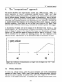
1.
Introduction. . . . . . . . . . . . . . . . . . . . . . . . . . . . . . . . . . . . . . . ., 7
2.
Edge detection . . . . . . . . . . . . . . . . . . . . . . . . . . . . . . . . . . . . . . .. 9
3.
t ' " approac h
Th e "1'me supporregIon
.
3.1
Image acquisition
3.2
Contrast operations
3.3
Filtering operations
3.4
Image segmentation . . . . . . . . . . . . . . . . . . . . . . . . . . . . . . . .
3.5
Line estimation . . . . . . . . . . . . .
3.6
Memory usage . . . . . . . . . . . . . . . . . . . . . . . . . . . . . . . . . . .
3.7
Conclusion.....................................
13
13
14
15
16
21
21
22
4.
The "computational" approach
4.1
Optimal detectors
4.2
Theory
4.3
Experiments
4.3.1 Implementation in Matlab
4.3.2 Implementation in C
4.4
Conclusion...............
23
23
24
32
32
35
37
5.
The "weak continuity constraint" approach
5.1
Detecting step discontinuities in 1D
5.2
The computational problem
5.3
Higher order energies: the weak rod and plate
5.4
Detection of discontinuities
5.5
Properties of the weak string and membrane
5.6
The minimisation problem
5.6.1 Convex approximation
5.6.2 The performance of the convex approximation
5.6.3 Descent algorithms
5.7
Stop criterion for the algorithm . . . . . . . . . . . . . . . . . . . . . . . . .
5.8
Experiments....................................
5.8.1 Implementation in Matlab . . . . . . . . . . . . . . . . . . . . . . . .
5.8.2 Implementation
5.9
Conclusion
39
39
40
45
46
47
48
48
51
52
54
54
54
58
61
6.
Line extraction
63
7.
Conclusions and recommendations
65
7.1
Conclusions............... . . . . . . . . . . . . . . . . . . . . . . 65
7.2
Recommendations
66
5
Contents
8.
References. . . . . . . . . . . . . . . . . . . . . . . . . . . . . . . . . . . . . . . . . . 67
Appendix A Program description ltLinefind.exe"
~
. .. . .
. . . . . . . . 71
Appendix B
Program description "Lee.exe"
77
Appendix C
Program decription "Wcc.exe"
79
6
Introduction
1.
Introduction
The Measurement and Control Section of the Department of Electrical Engineering of the
Eindhoven University of Technology is involved in the Esprit project 6042: "Intelligent
robotic welding system for unique fabrications", Hephaestos II [Esprit, 1992]. Goal of
this project is to define and produce a robotic welding system for a shipyard in Greece. In
the shipyard, ships are repaired by replacing damaged parts with new constructed ones.
The constructed ship-parts (workpieces) are unique and so far they have been assembled
and welded entirely manually. The aim of the project is to design and implement a
robotic welding system, which will replace most of the manual labour. Workpieces will be
assembled and tack welded manually. Then the Vision Survey System will extract a
geometrical description of the workpiece. This and other a priori knowledge from the
knowledge-base will be used to complete the welding job by the robotic system. The VSS
is under construction at this Section
The vision survey system is designed as follows: a set of cameras produces images of the
workpiece. These images are digitised to be processed by computer. From these images
lines are extracted that represent the physical contours of the objects. These lines serve as
an input for a 3-D reconstruction process. There are two types of reconstruction: top view
[Blokland, 1993] and side view [Staal, 1993]. The top view reconstruction uses data from
top view images and produces a rough model. This model is used, together with the data
obtained from the side view cameras, to generate the final 3-D geometrical data that can
be used for the welding process.
The task of the Master Thesis was to investigate a line segment extraction program
existing on a Sun system and to implement this on a Personal Computer. The accuracy of
the lines extraction should be improved and some properties of the line should be
determined along with the extraction. These properties could assist the decision making in
the reconstruction process.
This report describes the edge detection process, Le. the first step in the line extraction.
For the previous project Hepheastos I, a line extraction algorithm was implemented on a
Sun system [Farro, 1992]. From practical considerations the project Hephaestos II uses
personal computers, so this algorithm had to be transported. Also, to improve the two
reconstruction processes, more information about a line, particularly its environment, is
required. The "line support region" algorithm implemented by Farro [Farro, 1992] is not
suitable to extract this extra information. Therefore two other algorithms are investigated:
an algorithm proposed by Lee [Lee, 1988], [Lee, 1989] and a "weak continuity constraint" algorithm [Blake, 1987]. After detecting the edges, while preserving information,
the lines have to be extracted. Some algorithms to perform this are selected, but they are
not worked out.
7
Edge detection
2.
Edge detection
The main part of this report is concerning edge detection. In this section will be defined
what edge detection actually is. The framework, in which edge detection is used, is
described.
Machine Vision deals with processing camera images in order to control processes. To
control processes decisions have to be made. For example in a sorting machine, the
objects have to recognized, in order to guide them to the right place. Also in our
application, which is mainly a measurement task, objects have to be recognized. A
keyword in vision appears to be object recognition.
The object recognition needs references. It is possible to take a sample of one object, a
intensity value mask, and try to find the same pattern in other images. This is however a
very slow process, it requires convolutions with usually very large masks. It is also very
limited, in that it is not flexible. Varying lighting conditions, rotations of the objects are
hard to handle. When the objects are not known at all, it is completely impossible to use
this approach. What does this tell us? 1) The amount of data must be greatly reduced. 2)
A representation that is insensitive to lighting conditions, rotations, etc. must be found.
Feature extraction is one of the ways to achieve this. Contours of the objects are an
example of features. In vision edges are sudden changes in the intensity. These can result
from changes in the depth of the scene, changes in reflectance, etc. When these edges
could be extracted, a large reduction in the amount of data would be achieved [Hanajik,
1991]. consequently some knowledge is discarded, but a very useful part of the knowledge is contained in the edges.
Some definitions [Marr, 1980]:
•
•
An image is a projection of the 3-D scene onto a 2-D plane.
Edges I discontinuities of the intensity in the 2-D image are:
1
(sudden) changes in surface orientation in 3-D (edges)
2
(sudden) changes in surface reflectance (color, material)
3
(sudden) changes in surface illumination (shadow)
4
(sudden) changes in depth (contours, occluding boundaries)
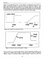
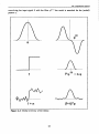
As said before, edges are changes in the intensity of the image. There can be sudden
changes: from one pixel to the next the intensity changes substantially, this is usually
called a step (figure 2.1a). It is also possible that the intensity of the pixels changes
approximately linear over a range of pixels. This is called a ramp. Assuming a consistent
grey level before and after the ramp (figure 2.1b), the transition can be considered an
edge or crease. The steps and creases are never ideal. This is caused by the camera
system. The camera system can be seen as a low pass system, edges and creases are not
sharp (figure 2.2). In theories about edge detection, quite often an approximation of steps
and creases is used. For the step edge this is the mathematical step, for the crease it is the
9
Edge detection
integral of the mathematical step. In some theories the mathematical step function is
called a discontinuity of degree Ot the ramp function a discontinuity of degree 1. Also
higher order discontinuities are possible t but in practice mostly zero and first order
discontinuities are used. In literature the term edge and discontinuity are used alternately.
In the description of the edge detection algorithms used, the choice of terms of the author
is followed, therefore discontinuity in this report is often used to denote edge.
1[\ grey
value
--J~---------?>
edge
a)
Figure 2.1: Example of a) step and b) ramp.
(neg)
step
'ramp
----I----Ir---------I---->----:7
edge edge
edge
Figure 2.2: Step and ramp as they appear in images.
There are several ways to perform edge detection. The three approaches described in this
report all use a different basic principle. In the direction across an edge, the change in
intensity is large, in the direction along the edge the change is usually very small. This
10
Edge detection
property is used by the "line suppon region" approach. When calculating the gradient of
the image, regions appear with approximately the same gradient direction. These regions
surround the line, therefore they are called "line support regions". When a region is
known a line can be estimated in it by a least squares estimator. This can be applied to
extract straight lines only.
The second approach is the use of filters to detect the edges. Over the years a huge
amount of filters have been developed. Canny [Canny, 1986] proposed some measures to
quantify the performance of a filter and described a computational way for a design of a
filter, optimizing these measures. Important performance measures of a filter are: 1)
sensitivity to noise, expressed by the signal-to-noise ratio, 2) localisation of the response,
3) the number of extrema (caused by noise) in the neighbourhood of the response to the
real edge. In a computational process, filters can be calculated for every type of edge that
must be detected. Lee [Lee, 1988] and [Lee, 1989] used this theory to optimize the filters
he designed. The filters designed by Lee are ment to detect discontinuities. For every
degree of discontinuity a different filter is derived. A special property of these filters is
that they are derivatives of some pattern. The (k+ 1)1h derivative of this pattern will return
that pattern as a response to a degree k discontinuity. (figure 2.3) Using statistical
properties of the responses it is possible to distinguish between true and false responses.
The third approach is to approximate the image by a piecewise continuous function.
Therefore the "weak continuity constraint" approach is developed [Blake, 1987]. For the
image a fit is calculated, using an energy function. This function contains terms expressing energy for the deviation from the real value, energy for deforming the fit, and a sum
of penalties for each discontinuity. The fit is calculated to be as smooth as possible. But
when the deformance of the fit becomes too high, it may be cheaper in terms of the
energy to put a discontinuity in that position. The penalty for the discontinuity must then
be lower than the energy caused by the deviation from the real values and the deforming
of the fit. The minimum energy fit is a piecewise continuous approximation of the
original image. The discontinuities in this approximation correspond accurately to the
edges in the image. An extension for detection of creases is also possible. The energy
must then be extended by a term representing energy for high curvature. This will make
second derivatives appear in the energy, causing very large computational effort,
compared to the first case. A different way to detect creases is then to calculate the first
fit. From this piecewise continuous approximation the derivative is taken, and for this
derivative another piecewise continuous approximation is calculated. The discontinuities in
this last approximation then correspond to the creases in the original image.
11
The "line support region" approach
3.
The "line support region" approach
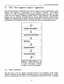
This section describes an algorithm that extracts straight lines from intensity (grey scale)
images. This algorithm is implemented in the program "Linefind". The program
'Linefind' is in fact a translation of the program Lowlevis [Farro], that runs on a Sun
system and uses Imaging Technology Series 150/151 Image Processor. The described
program runs on a Personal Computer (286 and up) and Data Translation 01'2851 Frame
Grabber and 01'2858 Auxiliary Frame Processor equipment. For this reason this section
concentrates on the differences between both programs, that are functionally the same.
image acquisition
contrast operations
filtering
segmentation
line estimation
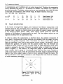
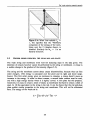
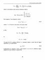
o
Figure 3.1: Block diagram of the
algorithm. i denotes the input, this
is a grey value image. 0 denotes
the ouput, a list of line segments.
3.1
IMAGE ACQUISmON
The first step in the line segment extraction process is the acquisition of the image.
Because computers process digital information only, the analog signal from the camera
has to be discretizised. The result is a two dimensional array (size 512x512), containing
13
The "line support region" approach
values representing the intensity in the range [0..255] of the part of the scene that is
projected on the array elements. From now on the array elements will be called pixels.
. The process from analog to digital infonnation is perfonned by the frame grabber. The
result is stored in one of the frame buffers provided by the frame processing equipment.
This is not different from 'Lowlevis', except for the names of the functions.
3.2
CONTRAST OPERATIONS
The library belonging to the Data Translation image processing equipment (DT-Iris) does
not provide ready-to-use functions for contrast enhancement. Probably the most common
contrast enhancement methods are linear stretching and equalization of a histogram. The
pixel values range from zero, for black, to 255, for white. Usually an acquired image
doesn't cover the full available range of intensity values. A histogram of an image assigns
to every intensity valuethe number of pixels having that value. The histogram contains
information about how the intensity values are spread over the available range. Often the
histogram is very low or zero near the ends and higher in the middle. To improve image
contrast, the pixel values of the image can be changed in such a way that the whole range
is used. If the function which maps original pixel values into new ones is linear, then the
operation is called "linear stretching". The image can also be changed in such a way that
all intensity values are equally used, this is a "histogram equalization". The linear stretch
just scales the image. For the oncoming parts of the algorithms the range of intensity
values should be as large as possible, for best performance. The linear stretch also avoids
changing the parameters discussed in appendix A, when lighting conditions change. The
histogram equalization is somewhat dangerous, as it deforms the histogram. This could
result in a contrast decrease at critical places. The histogram equalization is therefore not
implemented.
For the linear stretch, the 'feedback' function is used. This hardware function enables the
programmer to feed the image through a lookup table (LUT). The LUT contains for
every index, ranging from 0 to 255, a value. The values of the LUT can be programmed.
During the 'feedback' operation all pixels are passed through a specified LUT. The value
of a pixel is used as an index in the LUT. The pixel will then be assigned the indexed
value. To stretch the histogram of an image, this histogram is inspected and the minimum
and maximum intensity values that appear in the image are stored. Now a LUT is programmed. From index 0 to the minimum intensity value minus one and from the maximum
intensity value plus one to 255 the LUT values don't care as they are not present in the
image. Because the image doesn't have intensity values in those ranges no information is
lost. The indices ranging from the minimum to the maximum intensity value contain a
linearly increasing value, ranging from 0 to 255. (figure 3.2) When passed through this
LUT the resulting image has a better contrast. This operation takes about 2 seconds.
14
The "line support region" approach
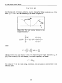
output
255
o
min
max 255
Input
Figure 3.2: Example of contrast enhancement function. On the dotted lines the values
don't care.
3.3
FILTERING OPERATIONS
Filters can be used for several purposes and in different domains. Because the program
uses single images, filtering in time domain is not possible. Filtering in spatial domain
can be very useful. If edges must be enhanced, high pass filters are commonly used. As
an ideal edge a step function can be considered. The spectrum of a step contains very
high frequencies. While all lower spatial frequencies are suppressed, the edges are
emphasized. Because an image can be considered as a low pass filtered signal, the energy
in the higher frequencies is less than in the lower frequencies. High pass filtering
therefore decreases the signal to noise ratio. Low pass filters increase the signal to noise
ratio by suppressing the higher frequencies. In practice the high pass filter is not used.
In 'Linefind' both high pass and low pass filters are implemented. For the high pass filter
a standard function is used. This function provides a 2-D convolution of the digital image
with a 3 by 3 kernel:
-1
-1
-1
-1
+9
-1
-1
-1
-1
For the low pass filter three Gaussian filters are implemented. The user can choose
between variances of 0.5, 2 and 4. The first filter reduces noise less than the other two,
but it keeps the image relatively sharp. The third filter gives a large noise reduction, but
also makes the image unsharp. For the Gaussian filters 7 by 7 kernels are used. These are
sampled versions of the continuous Gaussian filters. To increase speed these 7 by 7
Gaussian kernels can be decomposed into a 1 by 7 and a 7 by 1 kernel, yielding the same
results. These two kernels are then applied to the image in sequence. While the 7 by 7
kernel would require 49 multiplications and 48 additions per one output image pixel, the
1 by 7 and 7 by 1 kernels require just 7 multiplications and 6 additions each. That means
15
The "line support region" approach
14 multiplications and 12 additions per one output image pixel. Therefore the computation
time is decreased from about 15 - 20 seconds to 5 seconds. The variance of 0.5 seems to
give the best results. The higher variances give too much smoothing. Only when the noise
is very high, for example in a low contrast image, the higher variances were used.
The 7 by 1 and 1 by 7 kernels are:
(1 = 0.5
(1=2
(1=4
3.4
o
1
3
9
9
16
21
20
23
56
26
26
21
20
23
1
o
9
3
9
16
Scale factor: 100
Scale factor: 90
Scale factor: 122
IMAGE SEGMENrATION
In the vicinity of straight lines (edges), pixel values are very likely to change little in the
direction along the line and change much in the direction perpendicular to the line. This
property makes it possible to classify pixels into so called line suppon regions, according
to the intensity gradient [Bums, 1986]. These regions contain pixels for which the
direction of the gradient is approximately the same. The line support regions are the
segments resulting from the segmentation step.
In order to achieve the segmentation as described above, the gradient components of
every pixel in horizontal and vertical direction are calculated from the image. So every
pixel has two gradient component values. From these two values a vector length and an
angle are calculated. Every pixel is then assigned a sector number. The length is used to
threshold the gradients. All pixels with the gradient smaller than the threshold are
assigned the sector number zero. For all other pixels the angle determines which sector
number is assigned to the pixel. Therefore the gradient plane is divided into sectors as
shown in figure 3.3. This results in an image with groups of pixels having the same
sector number. Such a group of 4-connected pixels (with non-zero sector number) is
called a line suppon region. After the sectorization the whole image is searched for those
regions. Once a line support region is found, a line is estimated through that region. For
the line estimation a least squares estimator is used. Regions that were found are marked,
to avoid unnecessary processing.
r--"------------,
II
.... I ....
··m···
Figure 3.3: Possible division of
the gradient plane for image
segmentation
16
The "line support region" approach
A least squares estimator requires some data about the region: the accumulated sums of
the x-coordinates, the y~coordinates, the squares of the x- and y-coordinates and the
product of the x- and y-coordinates, of all pixels belonging to the region.
Both the programs 'Lowlevis' and 'Linefind' are based on the principle described above,
however the implementation differs significantly. Both programs scan the image line by
line and pixel by pixel to find points of line support regions. Once one point is found
'Lowlevis' uses a recursive algorithm to locate the complete line support region and at the
same time update accumulated sums. (Lowlevis had a user defined maximum depth of
3000 in order to find also large regions.) On the PC system this was not usable because
the stack space was not large enough. (With the default stack space a recursive depth of
only about 30 was reached, so on the PC system a complete recursive search would
require a too large stack.) Therefore a non-recursive algorithm was implemented. We call
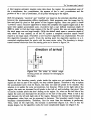
this algorithm boundary search. From the starting point the algorithm searches in a 4connected neighbourhood for pixels with the same sector value. The boundary is always
traced counter-clockwise from the starting point as in shown in figure 3.4.
direction of arrival
Figure 3.4: The order in which neighbouring pixels are checked for belonging to
the region.
Because of this boundary search, pixels inside the region are not reached (holes in the
region are seen as part of the region, but they seldom appear). Therefore a way to update
the accumulated sums must be found, that does not need all pixels to be reached. The
solution is to update the sums not pixelwise, but linewise. When on the right side of the
region, the sums are increased for all pixels to the left of, and including, that pixel. This
of course includes pixels that don't belong to the region. So, when on the left side of the
region the sums are decreased for all pixels to the left of that pixel. What is left is the
part between the left and right side of the region. Because the increase and decrease are
independent, other lines can be processed in between. The boundary search travels the
boundary counterclockwise. Therefore, first for most lines the decrease is performed.
Then, when on the right side, the increase is performed (figure 3.5). This is true for
simple shapes, but the algorithm works for more complicated shapes too (figure 3.6).
17
The "line support region" approach
subtract from accumulated sums
D
II
add to accumulated sums
pixel
pixel belonging to
region
Figure 3.5:: Calculation of accumulated sums
Figure 3.6: A more complicated shape, that
can still be handled by the boundary search.
18
The ·line support region· approach
For the updating process of the sums, some simple rules are used (figure 3.7).
.... . ....
.......
.......
......
...........
......
.............
.......
...
................ .
........
.............
•••
add(r)
add(r)
sub(r)
............................
....
..
.
.
.
..
...
.
,'
....
.
a
~
previous direction
(r)
-+-
new direction
Figure 3.7: The rules for the updating of the accumulated sums. Add(r)
means: add row value. Add(P) means: add pixel value. Sub(r) means:
subtract row value.
Updating formulas when on the left side of the region (sub(r». 'c' stands for the actual
column (x-direction) and 'r' stands for row (y-direction).
ndara
= ndara
19
- (c-l)
The "line support region" approach
c-l
EX-I>
Ex=
region
region
E y =L
region
y - (c-l) * r
region
Ex
c-I
2
y2
E x E ;2
2
=
region
E
laO
=
region
E
-
1-0
region
y2 - (c-l) * r 2
region
c-l
EX*y=EX*y-Ei*r
region
region
1-0
Updating formulas when on the right side of the region (add(r».
ndata = ndata + c
c
Ex = Ex + Ex
region
Ey=
region
Ex
region
1-0
region
Ey+c*r
region
c
2
=
L x + E;2
2
region
20
/-0
The "line support region" approach
L
region
y2 =
L y2 +
C
* r2
region
c
LX*Y= LX*y+I>*r
region
3.5
region
i-O
LINE ESTIMATION
The line estimator estimates a line through a line support region so that the sum of the
squares of perpendicular distances of region pixels to the estimated line is minimized. The
line is represented in the form: ax + by + c = O. The line could be represented using
only two parameters (a, b and c are not independent), but for the estimator it is more
convenient to use this representation. The vector [a b]T is the unit normal vector for the
line, this gives an easy expression for the distance of a pixel to the line.
From the pixel coordinates of the region the centroid is calculated. The estimator uses the
number of pixels in the region and the accumulated sums of x, y, x2, y2 and x*y. From
these sums the parameters a, b, c, AI and A2 are calculated. AI and A2 can be considered
estimates for the width and the length of the region. From the centroid and the length of
the region the begin and end point of the line can be calculated. These values are clipped
when they exceed image boundaries. This estimation differs from that in Lowlevis in that
Lowlevis uses two different parametrizations, depending on the sector number of the
regions. Lowlevis' estimator does not minimize the distance perpendicular to the line, but
the distance from a pixel to the line in horizontal or vertical direction, depending on the
parametrization used. Once a line is estimated, the begin and end points are stored in a
d2d format [Stap, 1992].
3.6
MEMORY USAGE
All operations up to the calculation of the horizontal and vertical gradient have been
performed using the Data Translation image processing equipment (by hardware). The
rest of the operations can not be performed on the image processing equipment, and the
image has to be transferred into the computer memory. This has caused a lot of problems.
The first problem was that the large memory model of the Microsoft C compiler does not
permit arrays exceeding 64 K of memory. Because Linefind uses 512 by 512 pixels for
one image, the memory required for one image is 256 K when intensity values are stored
as 'char'. To overcome the limited size the 'huge' qualifier was used. Although this
should enable the use of arrays exceeding 64 K, it didn't work. The solution to this
problem was to make an array of pointers, where these pointers were pointers to arrays.
Because in C arrays are treated as pointers, it was now possible to access an array
21
The "line support region" approach
element (representing one pixel) as if the array of pointers was a 2-dimensional array:
A[p][q].
At the same time another problem appeared. The program kept reporting memory
allocation errors, which were caused either by the Linefind program or by the Data
Translation device driver. The image processing equipment provides two frame buffers on
the board, but it supports up to 128 frame buffers, to be allocated in computer memory.
The extra frame buffers can be allocated using Data Translation library functions. The
extra frame buffers will be placed in extended memory. If this is not possible the buffers
are allocated in system memory. These buffers use 512 K of memory. Because Data
Translation does not support memory management standards it cannot use extended
memory. The memory manager used, QEMM386, takes all extended memory and passes
parts of it to programs requesting extended memory. While the Data Translation driver
cannot request extended memory it puts extra frame buffers in system memory. The extra
frame buffer was used to store intermediate results. The system memory is maximal 640
K, so there is no space for a frame buffer of 512 K, an array for images of 256 K and
the program itself. The solution was to store the intermediate results on a disk. This
decreases the speed of operation, but releases 512 K of system memory.
3.7
CONCLUSION
The transport of the program Lowlevis to a PC configuration contained some serious
traps, that took quite some time to overcome. Especially the size of the array to store
images caused a lot of trouble. On the other hand the Lowlevis program contained errors
and inaccuracies, which were solved. E. G. the line estimation was improved by not
minimising (in the least squares sense) the distances of the pixels to the line in horizontal
or vertical direction, but perpendicular to the line. At the same time the Linefind program
is more time and memory efficient, due to a better use of the special frame processing
equipment. The execution times of both programs are in the same order of magnitude. It
is impossible to give execution times, because these are dependent on the number of
regions in the image. They also depend on the control parameters described in appendix
A.
22
The ·computational· approach
4.
The" computational" approach
This section describes Lee's edge detection method [Lee, 1988] and [Lee, 1989], as a
special application of Canny's computational approach [Canny, 1986]. Lee's edge
detection method combines the detection, classification and measurement for discontinuities of different degrees. Herefore, for every degree of discontinuity, a filter is derived.
The result is a signal having extrema at the positions of the corresponding discontinuities.
Afterwards some statistical properties are determined for every extremum. According to
an ergodic theorem false responses can be distinguished from correct responses, using the
statistical properties. These filters, as well as those from Canny are I-D filters. They
should be used in different directions (e.g. horizontal and vertical) to process 2-D images.
A discontinuity of degree zero is the integral of the Kronecker delta function, a step
function (figure 4.1a). The discontinuity is located at the position of the step. A discontinuity of degree 1 appears in the integral of the degree zero discontinuity, and so on.
(figure 4.1b) The edges that appear in images are never as ideal as in figure 4.1. They
will be smoothed by the camera and digitizing process, but more important is the
influence of noise. Edge detectors can be optimized for edges in the presence of noise.
grey value
b)
a)
Figure 4.1: Definition of discontinuities: a) degree zero, b) degree one. The
the locations of the edges.
4.1
*
mark
OPTIMAL DETECTORS
To derive the optimal detector, within the given constraints, part of the computational
approach of Canny [Canny, 1986] is used. Canny specifies some performance measures
that can be used to calculate the optimal filter, given some weights for the measures.
They are: 1) the signal-to-noise ratio, 2) localisation and 3) distance between peaks in the
23
The "computational" approach
presence of noise. The signal to noise ratio is quite obvious: the ratio between the signal
part and the noise part of the response. Localisation and the distance between peaks
depend on the filter and will therefore be presented when the theory regarding the filter is
clarified.
Random noise
The theory make use of the ergodicity theorem, therefore a short recapitulation follows.
Two ways to calculate averages of stochastic processes are: ensemble average, average
the values of all member functions evaluated at a particular time and time average, the
average of a particular member function over all time. The ensemble average is denoted
as E{.} and the time average over the interval [- T, 1] as EIl-T , 1]{'}' A stochastic process is
ergodic if 1) the ensemble average is constant with time; 2) the time averages of all
member functions are equal; and 3) the ensemble and time averages are numerically
equal. White and Gaussian noise can be considered ergodic. From now on the noise is
considered ergodic.
An ergodic process is characterized by its autocorrelation function
Rn(t)
= neT) * n( -T) =
!
n(T)n(t+T)dT
where net) is a .... function at time t.
and power spectrum
Pn(S)
where N
= Fln]
Lemma 4.1. Let
4.2
= FIRn(t)] = N(s)N( -s) = I N(s) 12
and F is the Fourier transform.
~
(a filter) be a square integrable function. Then
THEoRY
The approach for finding discontinuities as proposed by D. Lee is: For degree kedges,
choose an appropriate pattern function tI', and then take the (k+ l)st derivative. After
24
The ·computational· approach
convolving the input signal S with the filter
pattern rp.
rp(1;+ 1)
the result is searched for the (scaled)
(n)
~
f
f*q>
f+n
(f+n)*q>
Figure 4.2: Global overview of the theory.
25
C.q>
The
·~omputational· approach
The convolution off and g is defined as
f* g(t) =
Jj(t-T)g(1)d1
-""
Obviously f"g
= g*J, f"(gl+ g~
= f"gl
+ f"g2
and erg)'
= f*g = f"g'.
The "computational" approach is based on the following theorem:
Theorem 4.1
Let the input signal f(t) have an ideal discontinuity of degree k at to with a base (to - L, to
+ L], where k = 0,1, ... and L>O. Let WkA, A), for r~O and A>O, be the set of real
valued functions satisfying the following conditions: i) it has absolutely continuous rn
derivative and square integrable (r+ 1).t derivative almost everywhere; ii) it has support
[-A, A), Le. it is identically zero outside the interval [-A, Al. Let ((J E Wt+l[-A, Al, where
O<A ~LI2. The convolution off and ((J(t+l) is:
Then for t E [-A, Al,
Proof:
For simplicity, assume that to = O. Then for k
T
~
0,
=f * ((J(t+l)
Since f is a polynomial of degree k in the interval [-L, 0),
f
is defined identical to that
polynomial in (-lXI, 0). Similarly, lis defined in [0, 00). Since
A) and O<A ~L12, for
t
E [-A, Al,
!*«((J)(t+\)
26
=
f"«((J)(t+\).
«((J)(t+l)
has support
[-A,
The ·computational· approach
Since
1(1:+1)
for
t
is a step function at 0 of size Il)(O+) _/l)(O_) and with infinite support,
1(1:+1)
= [fl)(O+)-.fl)(O-)]50
E [-A, A]
,where 50 is the delta function. Since 50*cp(t)
= cp,
0
In the presence of additive random noise
n: 1 = f+n , and with the appropriate choice
for a detector (cp, cp(l+I» for degree k edges, the filter response becomes
t =J * cp(l+l) = (f+n) * cp(l:+l) =f * cp(l+1)
+
n * cp(l+l)
Iff has an ideal discontinuity of degree k at to, then
(4.1)
where
T(tJ
=
fl)(t o+) _fl) (to - ) is the size of the discontinuity.
Theorem 4.1 suggests the following approach. When f has a degree k discontinuity at to
and cp has a feature point at 0 then T = cp has a feature point at to. Strict extremum is an
obvious choice as a feature point, and cp with a strict maximum at 0 is used. Therefore
extrema in the filter response are candidates for discontinuities.
To facilitate processing cp is chosen to satisfy:
i)
ii)
iii)
cp E W(l+lkA, A]
cp is symmetric and has a strict maximum at 0
cp is normalized (cp(O) = 1)
27
The "computational" approach
Optimal discontinuity detectors
From (4.1) the first part on the right side is the response to the signal f and the second
part is the response to the noise. The average magnitude of the extremum in the filter
response to the signal is proportional to E{ ~2(O)} = 1. The average magnitude of the
filter response to the noise is proportional to E{[n*~(.t+I)(to)]2}. From lemma 4.1 it is
invariant with respect to to. The signal-to-noise ratio is
E{~2(O)}
p =
E{[n *
~(k+I)]2}
The detector should be relatively insensitive to noise, therefore the signal-to-noise ratio
must be maximized.
The locations of extrema are used as candidates for discontinuities. The number of
extrema must be as low as possible, to avoid declaring false discontinuities. This is
equivalent to minimizing
or maximizing
/L
= E{[n * ~(k+1)]2}
E{[n
* ~(k+2)]2}
The detector ~ should maximize /L and p. For simplicity the product /LP is maximized.
From lemma 4.1
p.p
A
~
1
!
=- - - - - - - IFI~(l+2)](S) 12P,.(s)ds
minimizing the denominator of (4.2) must be found.
28
(4.2)
The ·computational· approach
Because of the noise, the location of an extremum in the filter response may deviate from
the actual location. The mean of this deviation is zero and the standard deviation of this
deviation, which has to be minimized, is:
! FI
I
E{;F} =
2
!p(t+2) (S)] 1 Pn(s)ds
(4.3)
[fA:) (0 +) -fA:)(O- )]2[!p1l (0)]2
The denominator of (4.2) and the numerator of (4.3) are equal. Therefore the optimal
detector also tends to minimize the deviation of the extremum in the filter response from
the location of the corresponding discontinuity in the input signal.
For white noise the denominator of (4.2) becomes
(4.4)
Minimization of (4.4) for the two most important cases: degree 0 (steps) and degree 1
(roof edges) results in the following filters:
For degree 0 discontinuities:
2
-t (2t+3A) + 1
A3
!p(t) =
2
-A~t~O
_t (2t-3A)+1
O<t~A
0
otherwise
A3
_ 6t(t+A)
A3
!p' (t) =
-A~t~O
6t(t-A)
A3
O<t~A
0
otherwise
29
The "computational" approach
0.03 .------,.~-,._---,._------,
0.02
o.e
0.01
0.6
0.4
-0.01
0.2
o
.
o
-0.02
so
150
-0.03 O~--~S.".O-....>O...O'---,
O
......O - - - - l ,50
Figure 4.3: Detector for degree zero discontinuities. The left plot is the pattern fP,
the right plot is the first derivative fP' .
For degree 1 discontinuities:
(t+A)3 (8t2-9At+3A 2)
3A s
fP(t)
(t-A)3 (8t2+9At+3A2) O~t~A
3A s
=
o
otherwise
20 (t+A)(8t2+At-A 2)
3A s
"l'
(t)
T
=
-A <t~O
-A ~ t< 0
20
2-At-A 2) O<t~A
-_(t-A)(8t
s
3A
o
otherwise
30
The "computational" approach
JlC10- 3
2r------,.----"""T"'""------,
-1
-2
-.3
.
o
50
100
150
Figure 4.4: The detector for degree 1 discontinuities. The left plot is the pattern rp,
the right plot is the second derivative rp".
Searching for the scaled pattern in the filter response
After the convolution, scaled patterns are searched in the filter response.
If/has an ideal discontinuity of degree k at to , then for t E [-A, A],
t'(..{o +t) - T(t~rp(l)
= n * rp(.t+I)(lo +t)
(4.5)
where T(loJ is the edge size.
If there is no noise, n =0, the matching is exact. When noise is present the matching is
approximate. Some ways to match the filter response and the scaled pattern are: calculate
the ~ or Lao norm of
(4.6)
If the norm is smaller than a threshold value, the matching is considered succesful.
However, the ~-norm tolerates sharp deviations and the Lao-norm seems to be too
conservative. Lee therefore suggests a statistical method based on the ergodic theorem
EIf_A,A,{[ittO+I)-T(I)CP(I)]} =E{n}! rp(k+l)(r)dr
EtI-A,A,{[T(lo+l) - itIO>cp(t)]2} =
31
!
(4.7)
IFlcp(k+1)](s)1 2Pn(s)ds
The "computational" approach
E'l.] denotes time mean, E{.} denotes ensemble mean,
Ft.] is the Fourier transform and PIt
is the power spectrum of n.
(4.5) Can be interpreted as an estimation of n*qp:+I}(to+t). For a correct discontinuity the
time mean and variance should approximately equal the right sides of (4.7), that can be
precomputed.
4.3
EXPERIMENTS
4.3.1 Implementation in Matlab
This theory has been implemented and tested using Matlab. Experiments are conducted on
single lines only, synthetic as well as real data. Routines that copy lines from the frame
grabber into Matlab variables, and vice versa, are available.
A single line is a one dimensional function of one coordinate space. However, the line the
camera produces is a function of time. So a line in the frame grabber can be considered a
function of time or space, whatever is more convenient. For the time mean El(.] the mean
over the area [-A,A] around t is taken.
In Lee's article functions <p are given as an example for zero or first order discontinuity
detection. The filters for zero order edge detection are implemented in Matlab. The
pattern <p used is a natural cubic spline and the corresponding filter cp' is a quadratic
spline.
2
-t
A3
<p(t)
(2t
+
3A)
= -(2t
t2
+ 3A)
3
A
0,
+
+
1,
1,
-A ~t<O
O~t$A
otherwise
The detection of extrema was in the first instance performed by calculating the zero
crossings of the first derivative of the filtered signal and using only the extrema that
exceed a certain threshold. This gives visually a good result. The locations of the extrema
match the edges in the image and there are almost no false responses.
The implementation of the ergodic theorem to distinguish false from correct responses,
did not give the results that were expected. Over the neighbourhood of an extreme, the
mean and variance of (4.6) are calculated. The same neighbourhood is used as in the
detection fase, this means [-A,A] with the extreme as centre. Comparing the results with
the mean of (4.6) from the response of the filter to noise only, it appeared that those
32
The "computational" approach
values did not match at all. The vanances were not compared in this stage of the
research.
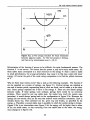
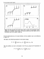
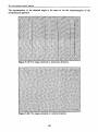
As test data a real image line (figure 4.6), an artificially made line, that resembles the
real one (figure 4.7), and the same artificial line with noise (uniformly distributed over [1,1]) (figure 4.8) were used. For the latter two cases the results are what the theory
predicts. As can be seen from Table 1 the extrema corresponding to real edges have
almost zero mean in the noiseless case, and a mean of about 0.05 in the case with added
noise. There are however a few outliers. This appears where two discontinuities are close
together. In this case they are separated by 6 or 7 pixels. With a support of 5 pixels to
either side for the filter this means that the responses of the two edges interact, and
thereby mess up the mean and variance of both.
From figure 4.6, the first extreme (position 4) and from figure 4.7 the third extreme
(position 168) are disregarded because they don't have matching extremes in the other
cases.
On the real line the location of the edges is determined with about one pixel accuracy,
however the values for the mean differs much from the artificial cases. This is because
the edges in the real line deviate too much from zero order discontinuities. This means
that the mean of (4.6) is not an estimate of the noise response to the filter, but it also
contains an estimate of the difference between real edge and ideal discontinuity.
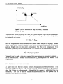
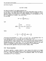
Figure 4.5: The image from which the line in figure 4.6 is taken.
(The line between the two black lines.)
33
The ·computational" approach
Lin_ 200;
A.
_
~
:zoo
-100
-200
:zoo
100
300
400
~oo
Figure 4.6: Upper trace: real image line, lower trace: filter response.
LIne
:zoo
1 00
200;
A
_
~
...r-,
~
o I-'-------...J
-100
-200
100
:zoo
300
400
~oo
Figure 4.7: Upper trace: a synthetic line, resembling the one in figure 4.6, lower
trace: filter response.
Line
200;
A
_
~
:zoo
1
00
~-------J--l
o I-'-------...J
-100
-200
100
200
300
400
~oo
Figure 4.8: Upper trace: the same synthetic line as in figure 4.7, with added noise,
lower trace: filter response.
34
The ·computational· approach
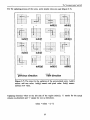
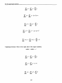
Table 4.1: Results for three lines.
position
Mean of (4.5) for
t E [-A, A]
T(la)
I
1
I
2
I
3
I
1
Var of (4.5) for
t E [-A, A]
2
3
1
2
3
1.16
4.36
3.51
122
22.2
19.2
19.4
-0.12
0.00
0.16
163
-71.3
-77.8
-17.8
1.06
3.36
3.28
181
13.1
10.6
11.4
0.51
0.00
0.11
2.46
1.57
1.60
219
16.9
16.3
16.5
1.52
0.00
-0.07
3.62
3.15
4.21
229
39.5
38.4
38.1
0.68
0.00
0.03
9.83
272
-56.0
-61.4
-62.0
4.27
4.15
4.22
278
19.5
18.2
18.8
-9.81
-8.38
361
39.9
27.8
28.2
1.83
0.00
-0.09
4.71
402
-66.3
-63.4
-63.9
-0.51
1.83
1.92
4.97
409
13.8
13.4
13.3
-6.71
-4.03
-8.68
432
65.7
63.4
63.4
5.07
0.00
-0.00
471
-29.6
-28.8
-28.4
-1.64
0.00
-0.04
-14.3
68.1
61.3
342
247
60.2
5.00
149
17.4
140
16.0
141
142
307
726
9.17
75.5
105
47.5
9.81
8.43
75.0
362
44.7
9.06
4.3.2 Implementation in C
Lee has developed the edge detector assuming some order ideal edges at the supporting
region [-A, A], contaminated with noise. In the response he searches for extrema and tries
to match them to the pattern that belongs to the filter, using that theory. It appeared from
the Matlab implementation that this matching was quite cumbersome and that just locating
all extrema and applying a simple threshold gives good results too. The program
lee. exe" , written in C, performs an edge detection on an image, using the theory of Lee,
except the stochastical matching. The advantage of using the filters developed by Lee,
even without the matching, is that they are designed for optimal localisation and maximum distance of extrema in the presence of noise. Furthermore the filters can be
implemented as convolutions at the D1'2858 Frame Processor. This combination gives
high speed and satisfactory accuracy.
II
Only detection of the edges is performed, the result are two intensity images. Where no
edge is present the value of the pixel is 128. A transition from light to dark (seen from
left to right or from top to bottom) appears dark in the intensity image. The contrast of
the edge is divided by two (to represent contrasts up to 255) and subtracted from 128. For
an opposite transition the value is added to 128. Due to scaling and the print process the
result may appear not very usable. The numerical data gives a good representation,
35
The 'computational" approach
however. There is no data present about the location of the edges. Because the edge
detector is 1-D the detection is performed once in horizontal direction and once in vertical
direction: Some results are:
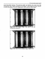
Figure 4.9: The image on which the edge detection is performed.
Figure 4.10: The edges detected in the horizontal detection.
36
The "computational" approach
Figure 4.11: The edges detected in vertical direction.
4.4
CONCLUSION
This is a fast and accurate edge detection algorithm. The edges that are detected are
stored in two frame buffers. The edges detected in vertical direction reside in frame
buffer 0, the edges detected in horizontal direction in frame buffer 1. The computation
time for the algorithm is about 21 seconds. This is the time between the moment of
freezing the image and the moment the results of both directions of detection are present.
37
The ·weak continuity constraint· approach
5.
The "weak continuity constraint" approach
Another way to detect lines in images is to obtain a piecewise continuous approximation
of the image. The resulting discontinuities in this approximation are the edges that were
detected. This piecewise continuous model can be obtained by fitting a spline to the data,
whilst allowing discontinuities when this would give a better fit. The "weak continuity
constraint" approach is one implementation of this theory. [Blake, 1987]
5.1
DETECflNG STEP DISCONTINUITIES IN
ID
To clarify the theory of weak continuity constraints, let's focus on a simple case: the
detection of step discontinuities in 10 data. Function u(x) will be fitted to the data d(x) in
a piecewise smooth way. The "weak elastic string" is an elastic string under weak
continuity constraints and will be used to model u(x). Discontinuities are places where the
continuity constraint on u(x) is violated. Such places can be visualised as breaks in the
string. The weak string is characterized by its associated energy. The problem of finding
u(x) is then the problem of minimizing that energy.
a)
b)
c)
--------------------~
.
Figure 5.1: Visualisation of the different elements of the energy. a) faithfulness to
the data (D). b) deforming energy (S). c) penalty for a discontinuity (P).
This energy is a sum of three components:
P:
the sum of penalties at levied for each discontinuity in the string (figure 5.lc).
39
The 'weak continuity constraint' approach
D:
a measure of faithfulness to the data. This can be visualised as minimising the
hatched area in figure 5. 1a.
S:
a measure of how severely the function u(x) is deformed. In figure 5.1b the dotted
line has lower energy S than the continuous line.
S can be interpreted as the elastic energy of the string itself. The constant >..,2 is a measure
of willingness to deform.
The goal is to approximate given data d(x) by the string u(x) , involving minimal total
energy:
E=D+S+P
Without the term P this problem could be solved using the calculus of variations. This
will clearly result in a compromise between minimising D and minimising S, a trade-off
between sticking close to the data and avoiding very steep gradients. The balance between
D and S is controlled by A. If A is small, D dominates. The resulting u(x) is a close fit to
the data d(x). A has the dimension of length and it will be shown that it is a characteristic
length or scale for the fitting process.
When P is included in E the minimisation is no longer a straightforward mathematical
problem. E may have many local minima. The reconstruction u(x) should yield the global
minimum. Depending on the values of a, A, and the height of the step h the resulting u(x)
contains a discontinuity, or is continuous.
5.2
THE COMPUTATIONAL PROBLEM
To implement this energy minimization problem on a computer, the problem has to be
discretisized. The continuous interval [0, N] is divided into N unit sub-intervals ('ele-
40
The ·weak continuity constraint· approach
ments') [0, l], ... ,[N-l, Nl, and nodal values are defined: uj = u(i) , i = O.. N. Then u(x)
is represented by a linear piece in each sub-interval. The energies defined earlier now
become:
N
S
= }..2E (u -Ui-I)2(1-1)
j
1
where Ij is a so-called "line process". It is defined such that each I j is a boolean-valued
variable. Ij = 1 indicates a discontinuity in the sub-interval [i-l,i], Ij = 0 indicates
continuity in that interval, Uj and uj _l are joined by a spring. When Ij = 1 the relevant
energy term in S is disabled.
The problem in discrete form is:
min E
{uj,/.}
The minimisation over the {/J can be done in advance, the problem then reduces to a
minimisation over the {uJ. This gives simpler computation, because it involves only one
set of real variables {uJ and the absence of boolean variables enables the "graduated nonconvexity algorithm" to be applied to minimize the energy E.
To eliminate the line-process {/J, E must first be expressed as:
N
E
=D
+
E ha,x(uj-ui-I' I
j)
i-I
where
and
41
The 'weak continuity constraint' approach
N
D
= L (U -d )2
o
j
j
as before. All dependence of E on the line-process is now contained in the N copies of
ha,>..' The function ha.,>.. controls local interactions between the {uj } .
The problem is now:
or
since D does not involve the {/j}' Now, immediately performing the minimisation over
{l;}, the remaining problem is to minimise F with respect to Uj , where
N
F
=D
+
L ga,>..(u -u
j
j _l)
(5.1)
I
and
ga>..
,
= IE{O,I}
min h
",(t,1)
a,
Explicitly ga,>.. is
if It I <~rA
otherwise
The central dip in the function ga,>..(t) (figure 5.2b) encourages continuity by pulling the
difference Uj - U j _1 between neighbouring values towards zero. The plateaus allow
discontinuity: the pull towards zero difference is released, and the weak continuity
constraint has been broken.
42
The ·weak continuity constraint· approach
1=0
....
h(t,l)
a.
....
1=1
--~----+---~~-_
t
a)
g(t)
...._-"
~-_
b)
...
t
Figure 5.2: a) The energy function for local interaction
between adjacent nodes. b) The line process I eliminated from a) by minimisation over I E {a, I}
Minimisation of the function F proves to be difficult, for quite fundamental reasons. The
function F is not convex. This means that the system uj may have many stable states. All
these stable states correspond to a local minimum in the energy F. Such a state is stable
to small perturbations, but a large perturbation may cause it to flip into a state with lower
energy. Of course the goal of the weak string computation is to find the global minimum
of F.
Why do these local minima exist? Take a look at the following example. The function F
can be regarded as a system of springs, see figure 5.3. Vertical springs are attached at
one end to anchor points, representing data di wich are fixed, and to nodes uj at the other
end. These springs represent the D term in the energy F. There are also lateral springs
between nodes. If these springs were ordinary springs there would be no convexity
problem. There would be just one stable state. No matter how much the system were
perturbed, it would always spring back to the configuration of figure 5.3a. However the
springs are not normal, they are the ones that enforce weak continuity constraints. Each is
initially elastic but, when stretched too far, gives way and breaks, as specified by the
energy g. Therefore a second stable state is possible in which the central spring is broken.
(figure 5.3b) In an intermediate state (figure 5.3c) the energy will be higher than in either
of the the stable states, so that traversing from one stable state to the other, the energy
must change as in figure 5.3d.
43
The "weak continuity constraint" approach
b)
a)
c)
l
d)
energy
a
c
b
Figure 5.3: Non-convexity: the weak string is like a system of conventional vertical
springs with "breakable" lateral strings. The states (a) and (b) are both stable, but the
intemediate state (c) has higher energy (d).
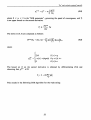
For the 2-dimensional case, the weak membrane, the line-variables 1 and m are defined as
in figure 5.4.
This leads to the following expression for the discrete energy:
The line-variables can also be eliminated in the 2D case, giving the 2D equivalent of
(5.1)
44
The "weak continuity conatraint" approach
Figure 5.4: When line-variable ljj =
1, this signifies that the "Northerly
component of the energy of the membrane over the 2 triangles shown, is
disabled. Similarly for mjj = 1 in an
Easterly direction.
5.3
HIGHER ORDER ENERGIES: THE WEAK ROD AND PLATE
The weak string and membrane work well for detecting steps in the data given. The
detection of creases however cannot be performed by the string or membrane. A crease is
a sudden change in the gradient of the intensity (figure 5.5).
The string and the membrane cannot detect crease discontinuities, because they use first
order energies. (The energy is calculated over the pixel and its right and lower neighbours.) This first order energy gives no resistance to creasing, a crease doesn't cause an
increase in the energy. In order to detect creases, a second order surface must be used,
one with a high energy density where it is tightly curved. A thin plate has this property.
Intuitively it is easy to crease a sheet of elastic (a membrane) but hard to crease a sheet of
steel. In ID the equivalent to the string is the rod. It can be shown that the rod and plate
plate exhibit similar properties to the string and membrane. This will not be elaborated
here. The energy of the weak rod is:
45
The "weak continuity constnint" approach
intensity
crease
position
Figure 5.5: The definition of step and crease, illustrated
for the IDease.
This involves a second derivative of u and will have a dramatic effect on the computational effort required to calculate the rod or plate. It is now also possible to include penalties
for both steps and creases:
P
= aZstep
+ {3Zcrease
Since the computational cost of schemes with second order energies is very high, another
way to obtain similar results is needed. It can be shown that the computation of the weak
plate can be split into two first order computations. The first is the computation of the
membrane, producing the step discontinuities. The surface can be differentiated to give:
This result can be used as data for a second first order process to reconstruct gradient PiJ
and its discontinuities. The step discontinuities in PiJ then represent the creases in the
original data.
5.4
DETECTION OF DISCONTINUITIES
As stated in § 5.2, the line process controls the appearance of discontinuities in the
optimal {uJ. When Ii (for the 2-D case also rnJ is 0, there is continuity in the interval,
when Ii is I there is a discontinuity. Although the line process is eliminated from the
calculation, it can still be used to indicate the discontinuities. The line process can be
recovered from g(t) by the formula:
46
The ·weak continuity constraint· approach
2 2
l = {A t
a
if ItI <";;fA
otherwise
The input t for g(t) is the difference between the two pixels that mark the interval l/.
The detection of the discontinuities is just ~rocess of checking if the difference between
fA.
two neigbouring pixels exceeds the value
va
s.s
PROPERTIES OF THE WEAK STRING AND MEMBRANE
So far the parameters a and A are arbitrary parameters, it is not clear what value they
should be assigned. Some properties will be presented here, for a derivation please refer
to [Blake, 1987].
q"
q"
q"
q"
q"
q"
The parameter A is a characteristic length.
The ratio ho = J2afA is a "contrast" sensitivity threshold, determining the minimum
contrast for detection of an isolated step edge. A step edge in the data is regarded
isolated if there are no features whithin A of it. This also clarifies the interpretation of
A as characteristic length. A is not only a characteristic length for smoothing the
continuous parts of the data, it is also a characteristic distance for interaction between
discontinuities.
When two similar steps in the data are only a apart ML~ A) they interact as follows:
the threshold for detection is increased by a factor VAfa compared with the threshold
for an isolated step.
The ratio gl = hJ2A is a limit on the gradient, above which spurious discontinuities
may be generated. When a ramp occurs in the data, with a gradient exceeding gl' one
or more discontinuities may appear in the fitted function.
It can be shown that, in a precise scene, location accuracy (for a given signal to noise
ratio) is high. In fact it is qualitatively as good as the "difference of boxes" operator
[Rosenfeld, 1971], but without any false zero-crossings problem. This means that there
is no problem determining which extremum in the response represents the actual edge.
Non-random localisation error is also minimised. Given asymmetrical data, gaussians
and other smooth linear operators make consistent errors in localisation. The weak
string, based as it is on least squares fitting, does not.
The parameter a is a measure of immunity to noise. If the mean noise has standard
deviation (1, then no spurious discontinuities are generated provided a> 2ci2, approximately.
47
The "weak continuity constraint" approach
d"
The membrane has a hysteresis property - a tendency to form unbroken edges. This is
an intrinsic property of membrane elasticity, and happens without any need to impose
additional coston edge terminations.
d"
The weak string and membrane are unable to detect crease discontinuities. This is
because a membrane conforms to a crease without any associated energy increase. To
detect creases a weak plate can be used.
5.6
TIlE MINIMISATION PROBLEM
The problem of finding the global minimum of F can not be solved by a local descent
algorithm, because of the non-convexity of F. A local descent algorithm is very likely to
get caught in a local minimum. There are several ways to overcome this problem. One of
them is the Graduated Non-Convexity Algorithm, from now on called GNC. The
algorithm consists of two steps. The first step is to construct a convex approximation to
the non-convex function, and then proceed to find its minimum. The second step is to
define a sequence of functions, ending with the true cost function, and to descend in each
in turn. Descent on each of these functions starts from the position reached by descent on
the previous one. In the case of the energy functions describing the weak string and
membrane it is even possible to show that the algorithm is correct for a significant class
of signals.
5.6.1 Convex approximation
The energy
N
F =D
+
E g(uj-u j_
l)
j-I
is to be approximated by a convex function
N
F'
=D
+
Eg ·(ui-uj-J)
i=1
by constructing an appropriate neighbour interaction function g.. This is done by
balancing the positive second derivatives in the first term D =
(u i -di )2 against the
negative second derivatives in the g* terms. The balancing procedure IS to test the Hessian
matrix H of F": if H is positive definite then F"(u) is a convex function of u. The Hessian
H of F" is
E,
48
The ·weak continuity constraint· approach
aF·
2
H .. = _ _ = 21.. + ~ g /I (U. -u._I)Q•.Q•.
IJ
auI auJ
~
LJ
IJ
A:
A
~,l
AJ
where I is the identity matrix and Q is defined as follows:
-1
=k
if i = k-l
o
otherwise
1 if i
QA:,I
= o(uA: -ut_I)/ou =
j
Now suppose g. were designed to satisfy
Vt,
where c·
g .11 (t)
~
-c·
(5.2)
> O. Then the "worst case" of H occurs when
vk , g.1I (u A: -ut-I ) = -c·
so that
or
To prove that H is posItIve definite, it is necessary simply to show that the largest
eigenvalue Vnuu of QTQ satisfies
V
~
max
2/c·
(5.3)
Construction of a function g. with a given bound c· as in (5.2) is relatively simple.
Suppose the extra condition is imposed that
49
The ·weak continuity constnint· approach
Vt, g • (t) < get)
then the best such g* (closest, pointwise, to g) is obtained by fitting a quadratic arc of the
form -~c· t 2 + bt + a to the function g(t), as shown in figure 5.6.
.... ~ g{t)
.
9 (t)
t
Figure 5.6: The local energy function g and
its approximation g•.
)..,2(t)2
ga\(t)
It1<q
if q$; It 1 <r
if It! ~r
if
= a -c • (I t l-r)212
where
All that remains now is to choose a value c· by determining the largest eigenvalue
QTQ. Then to satisfy (5.3) while keeping c· as small as possible, we choose
Vmax
of
c· = 2/vrnu.
The values of c· for the weak string, membrane, rod and plate are summarized in the
following table.
50
The ·weak continuity constraint" approach
Table 5.1: The values of c· for the different types of fits.
I
c•
string
1/2
membrane
1/4
rod
1/8
plate
1/32
I
5.6.2 The perfonnance of the convex approximation
Minimisation of F' is only the first of the two steps of the GNC algorithm. But just how
good is this approximation? Might it be sufficient only to minimise this? That depends on
the value of A. If A is small enough, it is sometimes sufficient. For larger A the second
step is essential.
When is the minimum of F', which can be found by gradient descent, also the global
minimum of F! For isolated steps and including noise some results can be given. In this
case F behaves exactly like F, except when the step height h is close to the contrast
sensitivity ho• How close depends on A. If A =1 then h must be quite close to ho before
F' starts to behave badly. But if A ~ 1 then F' behaves badly almost all the time. This
can be made intuitively clear by considering ga\' This approximates ga,>- only well for
small A. Hence F is much closer to F than when A is large.
A test for succes in optimising F' (in the sense that the minimum u· of F' is also the
global mimimum of F) is that:
(5.4)
g. is defined in such a way that
Vt, g ·(t) <g(t)
this means that
Vu, F· (u) < F(u)
Combining this with the definition of u·, that
51
The "weak continuity constraint" approach
and with (5.4) gives
Vu, F(u·) <F(u)
So when (5.4) holds u· is the global mimimum of F.
r was shown to be a good approximation to F, for the weak elastic string, for small A.
But for large A the second step of the GNC algorithm must be performed. A oneby
parameter family of cost functions p) is defined, replacing g. in the definition of
g(P). c· is replaced by a variable c, that varies with p.
For the string:
r
N
F(P)
=D
+
L g (P)(u -u
j
j
_
l
)
I
with
A2(t)2
g:~(t)
=
ItI <q
if q~ It I <r
if ItI >r
if
a-c(ltl-t)2/2
where
c
=
c· r 2 = a [2
p'
c+ A1]2 ,and q = Aa2r
At the start of the algorithm, p = I and c = c·, so g(l) =g • . As p decreases from I to
0, g(P) changes from g. to g. At the same time p) changes from
to F.
r
The GNC algorithm starts at minimising pi). This is the same as the convex function F'
and therefore has a unique minimum. From that minimum the local minimum of FP> is
tracked continuously as p varies from I to O. Of course discrete values of p are used.
Each JfJ') is minimised, using the minimum of the previous JfJ') as a starting point.
Proof that the GNC algorithm works can be found in [Blake, 1987].
5.6.3 Descent algorithms
As descent algorithm a gradient descend is used, because this proved to be highly
effective. A local quadratic approximation is used to determine the optimal step size. This
is in fact a form of non-linear successive over-relaxation (SOR). For the iterative
minimisation of p) the nib iteration is
52
The ·weak continuity constraint· approach
(ft+1)
U1
(ft)
= U1
-
1 aF(P)
T1 aUI
w---
(5.5)
where 0 < w < 2 is the "SOR parameter", governing the speed of convergence, and T,
is an upper bound on the second derivative:
The terms in (5.5) are computed as follows:
(5.6)
where
2}..2t
(p)1
ga,A
-
-
ItI <q
if q ~ It I <r
if ItI >r
if
-c( It I -r)sign(t)
o
The bound on T1 on the second derivative is obtained by differentiating (5.6) and
observing that g (p)1I ~ 2}"2
T1 = 2 + 2}..2E Q1.1
k
This results in the following SOR algorithm for the weak string:
53
The 'weak continuity constraint" approach
i Choose)., ho (scale and sensitivity).
ii Set ex ,;. hg)./2. iii Set SOR parameter: w =2(1-11),).
iv Choose p from function sequence: p E {1, 0.5, 0.25, ... , 11)" 1I2)'}.
v Use nodes: i E {O, ... ,N}.
vi For each p iterate n = 1, 2, ...
vii For i = 1, ... , N-1 compute
Uj(II+1)
= ut>
(5.7)
- w{2(ut>-dj)+g.?:i' (Uj(II)-Uj~;I)+g!.i' (ut)-u/~:)}/(2+4).2)
Appropriate modification is necessary at boundaries:
UJ"+l)
= uril)-w{2(uri"J-do>+g2:~' (uJ")-u 1(n»}/(2+2).2)
and similarly at i
5.7
= N.
STOP CRITERION FOR THE ALGORITHM
There are two locations in the algorithm at which a decision has to be taken to stop the
current iteration and the complete algorithm. The first location is at the descent-algorithm. Here a decision has to be taken to stop for the current approximation g(P), or not.
The implementation as in (5.7) has no explicit value for the energy F, so there are two
options for a stop criterion. 1) Calculate the energy F after each iteration and determine if
the minimum is reached, for example if the difference between the two iterations is lower
than a specified value. 2) Try to determine if the minimum is reached by observing the
individual updates. The first option is computationally more expensive of course.
The second location is the point where to determine if the global minimum is found. Here
has to be checked if (5.4) holds. If not, a better approximation for g(P) must be used. If
(5.4) holds the algorithm can stop. To check this, two energies F and F" must be calculated.
5.8
EXPERIMENTS
5.8.1 Implementation in Matlab
The theory described above was promising enough to implement it and evaluate it in Matlab. The algorithm for the weak string was implemented in Matlab. The implementation
consisted in fact only of a descend algorithm (SOR) for a fixed approximation for F. The
switch to a better approximation had to be made by hand. This was done to save
computing time. From the updates generated by the SOR algorithm, it was not clear when
54
The ·weak tontinuity tonstraint· approath
a minimum was reached. In fact a very small oscillation occurred, around the minimal
solution. This was probably caused by numerical aspects. It is possible that solution very
near to the optimal one, are numerically indistinguishable. Therefore the updates never
came to rest. It is of course possible to calculate the energy F and try to detect F reaching
a steady state, but this will increase the computational burden of the program.
As test-signals, real lines from a camera were used. The smoothing effect of the weak
string was very clear on the test signals. No attention was paid to the detection of
discontinuities in this phase of the research. From simple experiments it became clear that
the properties of the weak string as described above (§5.4) were met. Contrast sensitivity
h o accurately discarded steps below the sensitivity value. Also spurious step occurred
when the gradient of the intensity over the line exceeded g" This is a matter of concern
for the future. In real images, the data will almost never contain ideal steps with noise.
Because the data originates from a camera, a step will be somewhat smoothed. The step
in fact becomes a part in the data with a very large gradient. This results in spurious
responses, the large gradient will certainly exceed gr' While the transition is very steep
the generated steps will be very close to each other. In fact not a single step is found, but
an area of steps, lying next to each other.
intensity
detected edges
L-------'----'----'------'----'-----'~"_____'
__
jj----'----'___'___'I-----'I
_
position
Figure 5.7: Example of spurious responses on a very
large gradient. The straight line represents the data, the
dottet line the fitted string.
In figure (5.7) the detected edges are neighbouring pixels. The occurrence of such areas
must be handled by the line linking algorithm. The detected edge could be located for
example in the middle of the area, perpendicular to the direction of the edge.
Location of the step appears to be very accurate, within one pixel. The results for the
weak string in Matlab were very good. The implementation of the weak membrane was
not feasible in Matlab however. This is because of the enormous overhead, caused by the
communication with the frame grabber, and the size of the data. One image of 512 x 512
pixels requires about one Megabyte of memory, when every pixel is stored as a floating
point variable (4 bytes). The library of Microsoft C, version 7.0 contains some functions
55
The 'weak continuity constraint' approach
enabling the programmer to use very large datastructures. Therefore the weak membrane,
and also the weak string, was implemented using Microsoft C. This implementation is
also user guided, that means, the user determines the moments when to switch to a lower
value of p, and when to stop completely. The result of the operation is again an intensity
image. To help the user to determine how good the fit is, the profile of one line is also
displayed. The smoothing is much better visible in this profile, than in the intensity image
of the fit. The image can be used to detect the step edges. This is done in the same way
as described at the discussion of the Matlab implementation. The results of the fit are
very accurate, the location of the steps is within one pixel accuracy. The problem of the
non-ideal steps, caused by the vision-process, also arises here. The line linking algorithm
will have to take care of this, as this inherent to the weak continuity constraint algorithm.
In the next section the various properties of the weak string are illustrated on artificial
data. The length of the data is 20 elements.
The first figure (figure 5.8) shows the convergence of the algorithm. The data contains a
step of size 10 at element 11. The initial estimate for u is an array of zeros. In figure 5.8
only the first step of the GNC algorithm is executed. This means that only a minimisation
of F' is done.
, 0 r--~--~--~-----~---r---===
6
2
o!-~---------_I!II!!!!!!~ =--~_ _~_ _~_--:-,=--_----=,
o
2
4
6
e
Figure 5.8: The intermediate results for the first step of the GNC algorithm. The
initial estimate is all zeros. Ho is 5 and A is 4.
The next figure (figure 5.9) shows the effect of Ho on the performance of the GNC
algorithm. As data the same step is used as before, but homogeneously distributed noise
[-1,1] is added. The data is represented by a continuous line. The results u are represented by marks. The algorithm will only detect steps exceeding H o. Only for H o = 15 a
continuous spline is fit. The other three cases yield the same results.
56
The "weale continuity constraint" approach
'2 r--~--~--~--~--~---'---~--~--~------,
10
~_ . . ~. . . ~. . . . ~ . . . . ~ . . .
.........•.........
. . . . ,
·
8
;
6
":
:
:
:
~
~
":'"
;
.
"
4
.••.•••• ; .•.•••••••..••.••. : •.•..•••.
2
...•....
:
~·. . • . . . . . . . . . . • . . . . ~
,"
...... ..
o
, .
:
: :
.
'.
:
: .:
.
.:
.°a'"
•
.
':'
";_
":"
":"
·:
·
.
:
,
"...
~
.
.
.
. . . • . • . • .~ . . • • • • . . ~ . • • . • . • . • :• . • • • • . • • •: • • . . • . • • • ; • . • • . . . •
~.
d:
:
.
:
.
i
.~ ..•••..•• .~ . . • . . . . • . .~. . . . •...•.:.. . . . . . . • . .
: : . .
.:
.
~
-20~-----:2:-----':
...:--~6----=-a---:'''':'0---:-'''':'2--~'
":'"
... -_~,e::----'~8-------='20
Figure 5.9: Results of the GNC algorithm for various values of H o and fixed A = 4.
H o = 4: +, H o = 7: x, H o = 10: 0, H o = 15: •
Figure 5.10 shows the effect of interacting discontinuities. This is the effect that when
two steps are only a apart, and a ~ A, the threshold is increased by a factor l}Ja,
compared with the threshold for an isolated step. The data now consists of two steps of
size 10, located at element 7 and 13. Also the same noise is added to the data. The data is
represented by the continuous line. It is clearly visible that the results decrease when A
increases.
2~ r--~--~--~--~--~--~--~--~--~------,
·:
20
:
··
1 ~
: .•.......
.
.:
.:
.:
.:
;
;
;
;
:
:
i·········;·········:.········ .:
..
..
··
:
·
..
~ •••• ~ •••• OJ •••• ~
·
.
'0
~
~
..
.
...
..
..: . . . .
.
.
.
,
.
.
.. .
~ •••••••• ~
~
.
..
..
." :r::.......:l"::...-,.;;.;..---- '~.~
..-:-:..~.;
o
_~
:
2
__
...
L..-_~~_~
o
··
··
~
__
;
..
~
8
;
__
..
.
~
..
;
...
.
_ _---'-_ _
'0
'2
;
;.
...
:
:
;
..
;
..
..
r-:..-:-..~.*;-:...,.."
. ..,.....~.--:-.-.:..:-:
..~.i""'"'".",.i""'~''''
.,
.
-:.
..
,
..
.
..
:.
..
.
, ...
~
~.
..:.
.
~
'6
.
~
.
;
.
..
..
..
:
__
:
..
;.
__
..
.
..
~ _ - - - - - '
'8
20
Figure 5.10: Results of the GNC algorithm for various values of A and fixed H o =
5, to show the effect of interacting steps. A = 4: +, A = 6: x, A = 10: 0, A = 20:
•
The consequences of the gradient limit gl are visible in figure 5.11. Remember that
gl = hc!2A. The data now starts with 6 zeros. Than a slope, with a gradient of one,
occurs from element 7 up to 16, going from 0 to 10. The last elements have the value 10.
The value used for A is 4. When H o is 4, the gradient in the data (1) exceeds the gradient
limit (4/8) and a spurious step occurs (+). For H o is 8 (x) or 10 (0) no spurious steps are
generated, because the gradient limit is not exceeded. From this figure it is also visible
that the weak string fails to detect the creases.
57
The ·weak continuity constraint· approach
12
, 0
r--~--~--~--~--~--~--~--~--""""'---,
. . . . . • • • .: . . • . . . . . •
··
·
··
8
~
...••••..••..•........•••••
...
..
..
.
.
.
..
.
··
·
••...••• "
·
...... :
+
o
~
..
~
. '.
•
<
+
"
~
.
:.
+
~
:-.
:
.:
..
..
..
.
• . . . . ..
.
.
. .. ":
0:'.
0;".
":".
:'.
··
.
.
.
;, .. '."...
~
2
·
•
+
. ........
e·········:·········,·········
4
.
.
• • •
~
..
..
~
:
..
a
•••••••••••••••••••••••••
-:
..
"
..
.
.
••••••••
"
-:
:
~
..
.
.
-20~----:'2c--...----7~--~~----:1:"::·0---,~·2--~,.~... --~,.e-----i.,.8------l20
Figure 5.11: The effect of the gradient limit gl and the fact that creases are not
detected. A = 4:, Ho = 4: +, Ho = 8: x, Ho = 10: 0
The last figure (figure 5.12) shows the accuracy of the algorithm. The same step as in
figure 5.8 and figure 5.9 is used. The difference between the fitted curve and the original
step is plotted. For the continuous line, the fit to the noisy case is used. The dotted line is
the difference between the fit to the original step and the step itself. In the noiseless case
the fit is exact and in the noisy case the deviation is very small. The error does not show
a peak around the location of the edge. This means that there is no localisation error.
0.:55
0.3
0.25
0.2
O.,S
0.1
O.os
0
-O.os
0
2
",
4
20
Figure 5.12: The difference between the fit u and the data d for a noiseless and a
noisy step edge. The continuous line is for the noisy case, the dotted line for the
noiseless case.
5.8.2 Implementation in C
The programm "Wcc.exe" performs an edge detection on an image, using the weak
continuity constraint theory. It is implemented for manual control for switching and
stopping the algorithm. For evaluation of the algorithm this works fine. The implementation of the automatic stop of the descent algorithm by observing the individual updates did
not work. The updates never came to rest. It appears that a small oscillation occurs
58
The ·weak continuity coll8traint· approach
around the global minimum. The maximum update was therefore only rarely lower than
the specified value. Explicit calculation of the energy F would require too much calculation time, and therefore it was not implemented. Some results are shown below.
Figure 5.13: The original image. (The same as for the
computational approach.)
:b~
=;.tW
Figure 5.14: The fit for the original image. (figure 5.12)
59
The ·weak continuity constraint· approach
The representation of the detected edges is the same as for the implementation of the
computational approach.
Figure 5.16: The edges detected in vertical direction.
60
The ·weak continuity constraint· approach
5.9
CONCLUSION
The "weak continuity constraint" approach is a very elegant way of edge detection. It has
however some drawbacks, that make it less usefull in practice. The first one is the
computation time. It takes several minutes to calculate a good fit. Another drawback is
the fact that spurious responses are generated on steep slopes.
The edges that are detected are stored in two frame buffers. The strength of the edges is
imposed on a intensity value of 128.
61
Line extraction
6.
Line extraction
The task of the line linking process is to extract the detected edges by determining the
begin and end points of the line, and also some attributes. The edge detection processes
described before produce two kinds of information: the type and the strenght of the found
edges. The type of the edge is obvious: the type the filter is designed for. The strength of
the edge is the differce between values on opposite sides of the edge. The detectors detect
only edges of the "step"-type at the moment, but it is not very difficult to extend this. For
every type of edge there is information about the direction and size of the edge. For step
edges the size of the response represents the size of the step, for creases the size of the
response represents the change in the gradient and so on.
Before the lines can be extracted, some preprocessing might be advisable. It is possible
that a very small part of the edge is missed by the detector. By tracing the edge it is
possible to find such breaks. By checking the neigbourhood of such endpoint it is possible
to find the continuation of that edge. These parts can then be connected. The edges
produced by the "weak continuity constraint" algorithm can be more than one pixel wide.
This problem can be solved by taking the mean position in the direction perpendicular to
the direction of the edge.
The results of the horizontal and vertical edge detection must be combined of course. And
the properties of the edge must also be extracted. The value of the edge-pixels can for
example be used to detect comers, in addition to curvature. The value of the edge-pixel
gives information about its neighbourhood, and can therefore be helpfull in the line
linking process.
Because of the nature of both edge detectors it is not possible to use a "least squares"
estimator. This was possible for the "line support region" algorithm because regions (each
region represents one line) were constructed to be linear. Lines in different directions
could not be connected. The edges detected by the "computational" and the "weak
continuity constraint" algorithm can have any direction and can also be connected.
Therefore a line linking algorithm must be used that produces a piecewise linear estimation of the edge.
It is possible to extract the curve and then perform an angle detection. Rosenfeld
[Rosenfeld, 1973] and [Rosenfeld, 1975] describe an algorithm to perform this.
Williams [Williams, 1978] and [Williams, 1981] uses a different approach. This involves
the approximation of lines and curves by linear line segments that are constrained to pass
within specified distances of the points. The algorithm automatically selects line segments
as long as possible. This is not a "best fit" approximation. In fact, each approximated line
deviates from at least one data point by the maximum allowable amount.
Han, lang and Foster [Han, 1989] describe a split algorithm. The first estimation is one
line between begin and end point of the curve. Then the distance of the elements of the
curve to the line is determined. If this exceeds some value, the estimated line is split into
63
Line extraction
two lines. This procedure is repeated until all distances are smaller than the specified
value. The method described is efficient. A derivative-free line search method is applied
to determine the comerpoints of an image boundary.
64
Conclusions and recommendations
7.
Conclusions and recommendations
7.1
CONCLUSIONS
All algorithms described in the previous chapters were programmed in C and successfully
tested. For the "computational" and "weak continuity constraint" algorithms there is no
line linking yet. So comparison of the three algorithms is very difficult. The "line support
region" algorithm can, however, be judged at a pre line linking stage. All algorithms
produce images of the areas considered to be lines. These results can be visually
compared. The accuracy of the latter two algorithms appears to be far better than that of
the "line support region" algorithm. As said before, a real comparison can only be made
when the line linking for the other two algorithms is implemented.
The program "Linefind" is in fact a translation of the "Lowlevis" program, that was
implemented on a Sun. The performance of both programs is the same, the implementation required some major addaptions, because of the different natures of a Sun and a PC.
Edge localisation is not sufficient and also the algorithm offers no feature extraction
facilities, therefore it is rejected.
The program "Lee" is the implementation of the computational algorithm. This is a very
fast program to detect the edges in horizontal and vertical direction. The algorithm is onedimensional, so it must be performed in at least two directions. The resulting edges
appear to be accurately located. The number of spurious responses is very low. This
depends of course on the detection threshold. The number of missed edges is hard to
quantify. This is very dependend on the illumination and of course the detection threshold. The results of the program are good and the program needs only to be started, no
further operator intervence is needed to complete the edge detection.
The program "Wee" is the implementation of the weak continuity constraint algorithm.
The implementation consists of the basics of the theory. No actions are taken to stop the
algorithm automatically. The operator has to decide when to switch to a better approximation for the function g and when to stop completely. The calculation of a good fit can take
quite some time. The resulting edges are accurately located. The number of spurious
responses is higher than for the computational algorithm. This is mainly caused by the
multiple responses to a steep gradient. The fact is that most multiple responses are
connected, so it is not too hard to regard them as one response. The number of isolated
spurious responses is low. For the number of missed edges the same as for the computational approach holds.
All observations described above are based on the detection of degree zero discontinuities
(steps)
User manuals for the programs are included in appendices A-C.
65
Conclusions and recommendations
7.2
RECOMMENDATIONS
The program "Lee" works fine as it is, the program "Wee" can be improved: the
implementation of an automatic switch to a better approximation of g and an automatic
complete stop.
As stated in the conclusions, only detection for step edges is implemented. The detection
of higher order discontinuities is described in the theoretical chapters, but is not implemented. For this purpose only the function f{J needs to be changed in the computational
algorithm. For the weak continuity constraint algorithm the differential of the fit after the
step detection has to be taken. For the steps in this fit the differential should be set to
zero. From this differential the steps can be detected by calculating a new fit. The
discontinuities in the result are the creases in the original image.
Because the results of the computational and the weak continuity constraint algorithm are
in the same format, one line linking algorithm is likely to be usable for both.
For future use in the Esprit project the computational approach is recommended. This
approach gives good performance and has very acceptable speed. The filter operation can
be performed by convolution, and is therefore easy to implement. Also no user intervence
is needed, the algorithm needs only to be started.
66
Literature
8.
References
[Blake, 1987]
Visual reconstruction.
A. Blake, A. Zisserman.
Massachusetts: The MIT Press, 1987.
[Blokland, 1993]
Blokland, E.
3D workpiece reconstruction from 2D images.
M.Sc. Thesis, Eindhoven University of Technology, Measurement
and Control Section, april 1993.
[Bums, 1986]
Burns, J.B., A.R. Hanson and E.M. Riseman
Extracting straight lines.
IEEE Trans. on Pattern Analysis and Machine Intelligence, vol.
PAMI-8 (1986), no. 4, p. 425-455.
[Canny, 1986]
Canny, J.
A computational approach to edge detection.
IEEE Trans. on Pattern Analysis and Machine Intelligence, vol.
PAMI-8 (1986), no. 6, p. 679-698.
[Esprit, 1992]
Esprit Project 6042: Hephaestos II.
Technical Annex.
may, 1992.
[Farro, 1992]
Farro, M.J.
Straight line detection in low contrast images: Theory and application.
M.Sc. Thesis, Eindhoven University of Technology, Measurement
and Control Section, june 1992.
[Han, 1989]
Han, M.-H., D. lang and J. Foster.
Identification of cornerpoints of two-dimensional images using a line
search method.
Pattern Recognition, vol. 22 (1989), no 1, p. 13-20.
[Hanajik, 1991]
Hanajik, M.
Analysis of a line drawing of a workpiece.
Internal report, Eindhoven University of Technology, Measurement
and Control Section, november 1991.
67
Literature
[Lee, 1988]
Lee, D.
Coping with discontinuities in computer vision: their detection,
classification, and measurement.
IEEE second int. conf. on Computer Vision, 1989, Innisbrook
Resort, Tampa, Florida, USA, 5-8 december 1988.
P.546-557.
[Lee, 1989]
Lee, D.
Edge detection, classification, and measurement.
IEEE Computer Society Conference on Computer Vision and
Pattern Recognition, 1989, San Diego, California, USA, 4-8 june
1989.
P. 2-10.
[Marr, 1980]
Marr, D.C. and E. Hildreth.
Theory of edge detection.
Proc. Roy. Soc. London, vol. B 207 (1980), p. 187-217
[Rosenfeld, 1971]
Rosenfeld, A and M. Thurston.
Edge and curve detection for visual scene analysis.
IEEE Trans. on Computers, vol. C-20 (1971), no. 5, p. 562-569.
[Rosenfeld, 1973]
Rosenfeld, A and E. Johnston.
Angle detection on digital curves.
IEEE Trans. on Computers, vol. C-22 (1973), no. 9, p. 875-878.
[Rosenfeld, 1975]
Rosenfeld, A and J.S. Weszka.
An improved method of angle detection on digital curves.
IEEE Trans. on Computers, vol. C-24 (1975), no. 9, p. 940-941.
[Staal, 1993]
Staal, M.J .F.
Knowledge-based 3D workpiece reconstruction.
M.Sc. Thesis, Eindhoven University of Technology, Measurement
and Control Section, februari 1992.
[Stap, 1992]
Stap, J.W.
Automatic 3-D measurement of workpieces in a ship repair yard.
M.Sc. Thesis, Eindhoven University of Technology, Measurement
and Control Section, june 1992, p. 67.
[Williams, 1978]
Williams, C.M.
An efficient algorithm for the piecewise linear approximation of
planar curves.
Computer Graphics and Image Processing, vol. 8 (1978), p. 286293.
68
Literature
[Williams, 1981]
Williams, C.M.
Bounded straight-line approximation of digitized planar curves and
lines.
Computer Graphics and Image Processing, vol. 16 (1981), p. 370381.
69
I
Appendix A
Appendix A Program description "Linefind. exe"
User manual
System requirements
To use this program, a personal computer with the DT2851 frame grabber and the
D1'2858 auxiliary frame processor is needed. Also the Data Translation device driver,
version 01.05, must be loaded. The software is compiled using the DT-Iris library,
version 01.05. The software consists of the files 'LINEFIND.EXE' and 'IRIS.SET'. The
file "Iris.set" must reside in the active directory.
Operation
To run the program, 'LINEFIND' must be typed in the directory in which 'LINEFIND. EXE' resides. The program starts reading a setup file (see at 'IRIS.SET'). The
information is displayed for a moment. Then the frame processing equipment is initialized. The program tries to allocate 256 K memory for storage of an image. If the
allocation fails, the message 'Memory allocation failed' is displayed and the program
terminates. If the memory allocation if successful a menu is displayed.
< 1>
<2>
<3>
<4>
< 5>
<6>
<0>
Acquire image
Contrast operations
Filter operations
Sectorization
Line estimation
Retrieve image from disk
Exit program
Some of the menu options appear shaded. This means that they are not available at that
moment. For example, filter operations cannot be performed when no image is present.
< 1 > Acquire image
With this option an image can be acquired. The image will be displayed (real time) on the
monitor, so you can manipulate the scene and camera adjustments. When the image
appears ok, it is frozen by pressing any key.
< 2> Contrast operations
This option is only available when an image is acquired or loaded from disk. When the
image is acquired, the contrast is checked. If the range of intensity values used in the
image is less than 180, 'strongly recommended' appears behind this menu option. When
this option is chosen, a submenu appears.
< 1 > Linear stretching
< 2> Histogram equalization
< 0 > No stretching
71
Appendix A
< 1 > Linear stretching: The range of intensity values is linearly stretched.
< 2> Histogram equalization: This is not implemented.
< 3 > Filter operations
This option is only available when an image is acquired or loaded from disk. This option
gives a submenu
< 1 > High pass filter
< 2 > Gaussian filter
< 0 > No filtering
< 1 > High pass filter. The image is convolved with a 3 by 3 high pass kernel. This
emphasizes edges (or high frequencies in general), but also decreases signal to
noise ratio.
< 2> Gaussian filter. This option gives a submenu. There is a choice of one out of three
variances (0.5, 2.0 and 4.0). These filters are implemented as convolutions with a
7 by 7 kernel. (For considerations of speed this kernel is decomposed into a I by
7 and a 7 by I kernel.)
When the filter operation is performed the program asks if it should continue with the
filtered result (answer 'y' to the question), or with the image as it was before filtering
(choose 'n').
< 4 > Sectorization
This option is only available when an image is acquired or loaded from disk. When this
option is chosen, the program starts calculating gradients and determines to which sector
a pixel belongs. You can see this by the colour of the pixels on the screen. When the
whole image is processed, all pixels that don't have a neighbour (4-connectivity) with the
same sector number are removed. This will decrease the time needed for the line
estimation. The program asks if it should continue with the filtered result (answer 'y' to
the question), or with the unfiltered result.
< 5 > Line estimation
This option is only available when an image is acquired or loaded from disk and that
image is sectorized (menu option 4). When this option is chosen the program asks for the
name of the file to store the line information in. Then it starts searching for regions in the
sectorized image. When a region is completely detected, a line is estimated through it. All
estimated lines are shown on the screen.
< 6 > Retrieve image from disk
This option can be used to retrieve images from disk. The program can retrieve files that
are stored on disk with the Data Translation image processing equipment. When this
option is selected the program asks for the name of the file to be retrieved. The filename
can contain drive and path specifications.
72
Appendix A
Iris. set
This file contains parameters that influence the performance of the LINEFIND program.
IRIS.SET can be edited by any editor that operates on ASCII files. The first four
parameters define a work area in the image. The operations sectorization and line
estimation perform on the work area only. All other operations perform on the complete
image. The parameters are:
BEGIN X
This parameter of type integer defines the starting-point of
the work area in horizontal direction. (See fig. 1)
BEGIN Y
This parameter of type integer defines the starting-point of
the work area in vertical direction. (See fig. 1)
IMAGE- SIZE- X
This parameter of type integer defines the length of the work
area in horizontal direction. (See fig. 1)
IMAGE- SIZE- Y
This parameter of type integer defines the length of the work
area In vertical direction. (See fig. 1)
be~
I····.,--------·i
01
•
.§
:
OIl
~
end-y .
work area
•
. . . . .. '- -------. ---. -----. --------------.'
image
(512,0)
(512,512)
Figure A.I Definitions of image and work area. Pixel coordinates
are in (row,column)
ASPECT RATIO
MIN STEEPNESS
This parameter of type floating point reflects the aspect ratio
of the camera. (length in horizontal direction/ length in
vertical direction)
This parameter of type integer influences the image sectorization. MIN STEEPNESS is a threshold that must be
exceeded by the length of the gradient in order to be evaluated on direction. This parameter is defined in intensity
values/pixel. A higher value discards weaker edges. This
also implies that less regions are generated and as a consequence line estimation is less time consuming.
73
Appendix A
MIN- PIXEL- COUNT
MIN- LINE- LENGTH
This parameter of type integer defines the minimum number
of pixels a region must contain in order to estimate a line
through it. A higher value means that lines are only estimated in larger regions, which reduces processing time.
This parameter of type integer defines a threshold. Lines that
are longer appear in green on the screen. Lines that are
shorter appear in red. This has no influence on the lines
stored in the d2d-file.
Source code:
irissoft.c, irishard.c, iris.h
Executable file:
linefind.exe
Project file:
linefind. mak
Dependable file:
iris. set
Desciption of source files
The program consists of the source files irissoft.c, irishard.c and iris.h. Iris.h contains the
declaration of global variables. lrishard.c contains the routines that use the image
processing hardware and irissoft.c contains all other routines, including the main routine.
The routines are shortly decribed below.
Irissoft.c
clear screenO
This function clears the text screen. Ansi.sys needed.
setupO
This function reads the default values in the file 'iris. set' and opens
a file for use as d2d-file.
IsJine_estimationO
Least square estimation of a line through the last found region. This
function returns 0 if the number of pixels if below a specified
bound. It returns 1 if a line is estimated.
draw_foundJineO
This function draws the last found line and writes coordinates to d2d
file.
positionO
This function returns the value of the neighbour of point
(row,column) indicated by 'dir' or 0 if neighbour(dir) out of work
area.
find_nextyointO
This function searches the next point on the boundary of a region
with the value 'value'. It searches for a 4-connected neighbour of
the point (row,column) using the direction of arrival. The direction
of the found neighbour is passed also via 'dir'. Neighbour value is
'anded' by 63 to get rid of boundary mark (value + 64).
74
Appendix A
add to sumO
This function is used to update running sums for new point.
subtract_from_sumO This function is used to update running sums for new point.
This function is used to update running sums for new point. The
previous direction is used to determine if update is needed. On the
left side of the region a value is subtracted, on the right side added.
This function searches for the boundary of a region with value
'value', starting from point (row,column).
find_sectorO
This function is used to find a region in the image.
finish d2d fileO
This function completes the d2d-file.
gradient20
This function calculates the gradients and assigns a sector value to
each pixels according to the gradient. Changes FB 0 and 1.
Irishard.c
initializeO
This function initializes the DT2851 frame grabber. It also creates a
frame buffer in the memory of the computer.
linearizeO
This function linearizes the histogram of an image, stored in frame
store O. The range is linearized between 'min' and 'max'. The
result is stored in FB O.
grab)mageO
This function grabs the image and stores it in frame store O. Returns
1 if contrast enhancement needed, else O.
contrastO
This function performs contrast operations on the image in frame
store O. The result is stored in frame store O.
filterO
This function performs filter operations on the image in frame store
O. You can choose to continue with the result or with the original
image. This image is stored in frame store 1.
gradientO
This function calculates the gradient of the image in frame store 0,
and assigns sector numbers according to it. Result in frame store O.
Frame store 1 changed.
sectorizeO
This function divides an image into sectors. This is done by passing
the image through a LUT. Result in FB O.
75
Appendix A
removeyixel_noiseO
This function removes isolated pixels from a segmented
image. It should not contain more than 8 sectors. The oper. ation· is done in hardware. A 4-neighborhood is used. (To
use up to 16 sectors the data should be loaded from the
frame processor in two steps (high and low byte» Position
coding is used. Result in FB 0, Fb1 changed.
76
Appendix B
Appendix B Program description "Lee.exe"
User manual
The program lee.exe performs an edge detection on an image, using part of the theory of
D. Lee. Lee has derived filters for different types of discontinuities. These filters are
differentials of some order of a spline. The order of the differential depends on the order
of the discontinuity to be detected. When such a filter is convolved with a signal
containing the type of discontinuity the filter was intended for, the original spline will
return in the response. This (scaled) spline can be extracted from the response, in order
to find the location of the edge. Lee developed a theory about determining if the response
is a proper one. In the response he searches for extrema and tries to match them to the
spline, using that theory. It appeared that this matching was quite cumbersome and that
just locating all extrema and applying a simple threshold gave good results too. The
advantage of using the filters developed by D. Lee is that they are designed for optimal
localisation and maximum distance of extrema in the presence of noise. Furthermore the
filters can be implemented as convolutions at the DTI858 Frame Processor. This
combination gives high speed and great accuracy.
System requirements
To use this program, a personal computer with the Data Translation DTI8S1 frame
grabber and the DTI858 auxiliary frame processor is needed. The Data Translation
device driver must be loaded (version 01.05). The program is compiled using the DT-Iris
library version 01.05. The program needs the files "Lee.exe" and "Lee.set" to run.
"Lee.set" must be in the active directory.
Operation
The program starts with a message to press a key to freeze the image. Set up the scene as
wanted and press a key to freeze the image. Some messages will appear about allocation
of memory. The user should only be aware of it when the allocation fails. In that case the
program terminates immediately. When the allocation succeeds the program will start
detecting the edges in horizontal direction. The results are visible on the vision monitor.
Then the detection in vertical direction will take place. When this is also finished, the
edges in horizontal and vertical direction can be displayed alternating on the vision
monitor. Each time a key is pressed the other edge-image is displayed. Pressing's' once
or twice (depending on what image is displayed that moment) will end the program.
Lee.set
The program reads a setup file ('lee. set'). This file contains two parameters that control
the program operation.
A
The length of the spline (the width of the filter) can be adjusted by A. This
will give a spline of 2A + I elements [-A, + A]. A must be an integer. When
two edges are separated less than 2A, they will interact.
77
Appendix B
DELTA
This is the detection threshold. The peak value of the response must exceed
this value, to make it appear in the result.
Source code:
lee.c
Executable file:
lee.exe
Project file:
lee. male:
Dependable file:
lee. set
Description of the source file
This file contains the complete program. The functions that are used by the program are
shortly described below.
initializeO
This function initializes the DT28S1 frame grabber. It also creates a frame
buffer in the memory of the computer.
setupO
This function reads the default values in the file 'lee. set' .
draw lineO
This function draws one image line on the computer screen.
signO
Sign function: returns 1 if inp is positive, 0 if zero and -1 if negative.
find_edgesO
This function performs the actual edge detection (l dimension). Result in
frame buffer O.
78
AppcndixC
Appendix C Program decription "Wcc.exe"
User manual
The program wcc.exe performs an edge detection on an image, using the theory of weak
continuity constraints. This means that the original image will be approximated by a
discretisized spline. This spline is constructed to have a minimal energy (in the sense of
difference of a pixel to its neighbours and to the value of the original). The spline has an
extra property in that it allows discontinuities when the difference becomes to high. These
discontinuities coincide almost exactly with real edges, and that makes it suitable as edge
detector.
System requirements
To use this program, a personal computer with the Data Translation DT285 I frame
grabber and the DT2858 auxiliary frame processor is needed. The Data Translation
device driver must be loaded (version 01.05). The program is compiled using the DT-Iris
library version 01.05. The program needs the files "Wce.exe" and "Wec.set" to run.
"Wee.set" must be in the active directory.
Operation
The program starts to asks for two values: lambda and hO. These will be explained later.
The program continues with some messages about the allocation of memory. The user
should only be aware of it when the allocation fails. In that case the program terminates
immediately. When the memory allocation succeeds,J a menu will appear with seven
options.
1.
2.
3.
4.
5.
6.
O.
Acquire image. Use this option to grab an image from the camera.
Weak. string. This option will show the result of the weak. continuity constraint
method on a single image line (l dimensional). This gives some insight in the
quality of the algorithm. Press a key to decrease the value of 'p'. CP' is a measure
for the quality of the fit.) Press's' to stop the algorithm and return to the menu.
The algorithm will not decrease 'p' or stop by itself.
Weak. membrane. This is the 2-dimensional implementation of the weak. continuity
constraint method. Pressing a key will also decrease 'p' and pressing's' will stop
the algorithm. This may take some time because keystrokes are only evaluated
after one complete iteration. The algorithm will not decrease 'p' or stop by itself.
Edge detection. This option will locate all discontinuities and display them. A
difference to its right and lower neighbour greater than hO is considered a discontinuity. Press a key to return to the menu.
Restore previous result of the membrane. The last calculated spline is loaded, and
can be used for further elaboration. The result of the previous calculation is stored
as ·wec. img' .
Change the values of lambda and hO. The values of lambda and hO can be changed
to calculate a new spline.
Exit. Leave the program.
79
AppendixC
Parameters
Lambda:
hO:
This float parameter is a measure for the width of the filter. A large
lambda will give faster convergence, but also a smoother spline. It will be
harder to find the edges. A smaller lambda will give sharper discontinuities. A value of 4 gives good results.
This integer parameter controls the appearance of discontinuities in the
spline. This difference between two neighbours is restricted by an energy
function. The larger the difference, the larger the (elastic) energy. The
algorithm tries to minimize the total energy of the spline, that consists of
the difference between spline and original and the elastic energy of the
spline itself. The energy function is monotonically increasing, up to the
difference hO. From then on it has a constant value Ot. When fitting the
spline to a step, a continuous spline will have high differential energy and
low elastic energy. When the energy of the spline for the step is higher
than Ot, it is cheaper to accept the discontinuity. This will give an energy of
Ot for the discontinuity and almost zero differential energy. This can only
occur when the size of the step exceeds hO.
Wee.set
The program reads a setup file ('wcc.set'). This file contains three parameters that control
the output in the weak membrane section.
DISPLAY RESULT:
DISPLAY INTERVAL:
LINE NUMBER:
When this parameter is set to one, the result of the iterations
will be shown, depending on DISPLAY_INTERVAL. When
set to zero, the result is only displayed at the beginning of
the algorithm and when 'p' is decreased.
When DISPLAY_RESULT is one, this parameter controls
how often the result is displayed. This will occur every
DISPLAY INTERVAL iterations.
The effect of the algorithm is very perceptible in a single
line projected on the screen. LINE_NUMBER controls
which line will be projected on the screen.
Source code:
wcc.c
Executable file:
wcc.exe
Project file:
wee. male
Dependable file:
wee. set
80
AppendixC
Description of the source file
This file contains the complete program. The functions that are used by the program are
shortly described below.
setupO
This function reads the default values in the file 'wee. set' .
initializeO
This function initializes the DT2851 frame grabber. It also creates a
frame buffer in the memory of the computer.
signO
Sign function: returns 1 if inp is positive, 0 if zero and -1 if negative.
This function generates a table representing the g-function, for
specified lambda, hO and p, for the weak string.
make_membrane_dgO
This function generates a table representing the g-function,
for specified lambda, hO and p, for the weak membrane.
draw_lineO
This function draws one image line on the computer screen.
vdrawJineO
This function draws one image line from virtual memory on the
computer screen.
draw_imageO
This function draws a grayscale image on the computer screen.
copyJmage_from_fg_to_vmO
This function copies one image from the frame buffer
o to virtual memory.
weak_stringO
This function calculates the weak string.
weak_membraneO
This function calculates the weak membrane.
detect_edges()
This function performs actual edge determination.
81