Download LabTalk Scripting Guide

LabTalk Programming Guide for
Origin 8.5.1
Table of Contents
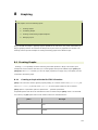
1
LabTalk Scripting Guide....................................................................................... 1
2
Introduction ........................................................................................................ 3
3
Getting Started with LabTalk............................................................................... 5
3.1
Hello World ..................................................................................................................... 5
3.1.1
3.1.2
3.2
3.3
3.4
Script Window .............................................................................................................5
Custom Routine ...........................................................................................................5
Hello LabTalk................................................................................................................... 6
Using = to Get Quick Output .............................................................................................6
Working with Data ...........................................................................................................7
3.4.1
3.4.2
3.5
4
Input and Operators.....................................................................................................7
Import........................................................................................................................8
Where to Go from Here? ...................................................................................................8
Language Fundamentals ....................................................................................11
4.1
General Language Features ............................................................................................. 11
4.1.1
4.1.2
4.1.3
4.1.4
4.1.5
4.1.6
4.2
Data Types and Variables............................................................................................ 11
Programming Syntax.................................................................................................. 21
Operators ................................................................................................................. 27
Conditional and Loop Structures .................................................................................. 34
Macros ..................................................................................................................... 38
Functions .................................................................................................................. 40
Special Language Features .............................................................................................. 47
4.2.1
4.2.2
4.2.3
4.2.4
4.2.5
4.2.6
4.3
5
Range Notation.......................................................................................................... 47
Substitution Notation.................................................................................................. 57
LabTalk Objects ......................................................................................................... 67
Origin Objects ........................................................................................................... 70
String registers........................................................................................................ 124
X-Functions............................................................................................................. 129
LabTalk Script Precedence............................................................................................. 130
Running and Debugging LabTalk Scripts ..........................................................131
5.1
Running Scripts ........................................................................................................... 131
5.1.1
5.1.2
5.1.3
5.1.4
5.1.5
5.1.6
5.1.7
5.1.8
5.1.9
5.1.10
5.1.11
5.1.12
5.1.13
5.1.14
5.1.15
5.2
5.2.1
5.2.2
5.2.3
6
From Script and Command Window............................................................................ 132
From Files ............................................................................................................... 133
From Set Values Dialog............................................................................................. 138
From Worksheet Script ............................................................................................. 139
From Script Panel .................................................................................................... 140
From Graphical Objects ............................................................................................ 140
ProjectEvents Script ................................................................................................. 142
From Import Wizard ................................................................................................. 143
From Nonlinear Fitter ............................................................................................... 144
From an External Application ..................................................................................... 144
From Console .......................................................................................................... 145
On A Timer ............................................................................................................. 150
On Starting Origin.................................................................................................... 151
From a Custom Menu Item........................................................................................ 153
From a Toolbar Button.............................................................................................. 153
Debugging Scripts ........................................................................................................ 156
Interactive Execution................................................................................................ 156
Debugging Tools ...................................................................................................... 157
Error Handling ......................................................................................................... 162
Working With Data ...........................................................................................165
6.1
Numeric Data .............................................................................................................. 165
iii
LabTalk Programming Guide for Origin 8.5.1
6.1.1
6.1.2
6.2
6.2.1
6.2.2
6.2.3
6.2.4
6.3
6.3.1
6.3.2
7
7.1.1
7.1.2
7.2
7.2.1
7.2.2
7.3
7.3.1
7.3.2
7.4
String Variables and String Registers.......................................................................... 168
String Processing ..................................................................................................... 169
Conversion to Numeric ............................................................................................. 171
String Arrays........................................................................................................... 172
Date and Time Data ..................................................................................................... 172
Dates and Times ...................................................................................................... 173
Formatting for Output .............................................................................................. 174
Worksheet Manipulation ................................................................................................ 177
Basic Worksheet Operation ....................................................................................... 177
Worksheet Data Manipulation .................................................................................... 180
Matrix Manipulation ...................................................................................................... 183
Basic Matrix Operation.............................................................................................. 183
Data Manipulation .................................................................................................... 185
Worksheet and Matrix Conversion .................................................................................. 189
Worksheet to Matrix ................................................................................................. 189
Matrix to Worksheet ................................................................................................. 189
Virtual Matrix............................................................................................................... 190
Graphing ..........................................................................................................193
8.1
8.1.1
8.1.2
8.1.3
8.1.4
8.2
8.2.1
8.2.2
8.2.3
8.2.4
8.2.5
8.2.6
8.3
8.3.1
8.3.2
8.3.3
8.3.4
8.3.5
8.3.6
8.3.7
8.3.8
8.4
8.4.1
8.4.2
8.4.3
9
String Processing ......................................................................................................... 168
Workbooks and Matrixbooks ............................................................................177
7.1
8
Converting to String ................................................................................................. 165
Operations .............................................................................................................. 167
Creating Graphs........................................................................................................... 193
Creating a Graph with the PLOTXY X-Function ............................................................. 193
Create Graph Groups with the PLOTGROUP X-Function ................................................. 195
Create 3D Graphs with Worksheet -p Command .......................................................... 196
Create 3D Graph and Contour Graphs from Virtual Matrix ............................................. 197
Formatting Graphs ....................................................................................................... 197
Graph Window......................................................................................................... 197
Page Properties ....................................................................................................... 197
Layer Properties ...................................................................................................... 198
Axis Properties ........................................................................................................ 198
Data Plot Properties ................................................................................................. 199
Legend and Label..................................................................................................... 199
Managing Layers .......................................................................................................... 200
Creating a panel plot ................................................................................................ 200
Adding Layers to a Graph Window.............................................................................. 200
Arranging the layers................................................................................................. 201
Moving a layer......................................................................................................... 201
Swap two layers ...................................................................................................... 201
Aligning layers......................................................................................................... 202
Linking Layers ......................................................................................................... 202
Setting Layer Unit .................................................................................................... 202
Creating and Accessing Graphical Objects ....................................................................... 202
Labels .................................................................................................................... 202
Graph Legend.......................................................................................................... 204
Draw ...................................................................................................................... 205
Importing.........................................................................................................207
9.1
9.1.1
9.1.2
9.1.3
9.1.4
9.1.5
9.1.6
9.1.7
9.2
Importing Data ............................................................................................................ 209
Import an ASCII Data File Into a Worksheet or Matrix .................................................. 209
Import ASCII Data with Options Specified ................................................................... 209
Import Multiple Data Files ......................................................................................... 210
Import an ASCII File to Worksheet and Convert to Matrix ............................................. 210
Related: the Open Command .................................................................................... 210
Import with Themes and Filters ................................................................................. 211
Import from a Database ........................................................................................... 211
Importing Images ........................................................................................................ 213
iv
Table of Contents
9.2.1
9.2.2
9.2.3
9.2.4
Import
Import
Import
Import
Image to Matrix and Convert to Data ............................................................... 213
Single Image to Matrix ................................................................................... 213
Multiple Images to Matrix Book ....................................................................... 213
Image to Graph Layer .................................................................................... 214
10 Exporting .........................................................................................................215
10.1
Exporting Worksheets................................................................................................... 215
10.1.1
10.2
10.2.1
10.2.2
10.2.3
10.3
Export a Worksheet.................................................................................................. 216
Exporting Graphs ......................................................................................................... 217
Export a Graph with Specific Width and Resolution (DPI) .............................................. 217
Exporting All Graphs in the Project ............................................................................. 217
Exporting Graph with Path and File Name ................................................................... 218
Exporting Matrices ....................................................................................................... 218
10.3.1
10.3.2
Exporting a Non-Image Matrix ................................................................................... 218
Exporting an Image Matrix ........................................................................................ 218
11 The Origin Project ............................................................................................221
11.1
Managing the Project .................................................................................................... 221
11.1.1
11.1.2
11.2
Accessing Metadata ...................................................................................................... 224
11.2.1
11.2.2
11.2.3
11.3
The DOCUMENT Command........................................................................................ 221
Project Explorer X-Functions ..................................................................................... 223
Column Label Rows .................................................................................................. 224
Even Sampling Interval ............................................................................................ 225
Trees...................................................................................................................... 226
Looping Over Objects ................................................................................................... 229
11.3.1
11.3.2
Looping over Objects in a Project ............................................................................... 229
Perform Peak Analysis on All Layers in Graph .............................................................. 233
12 Calling X-Functions and Origin C Functions ......................................................235
12.1
X-Functions ................................................................................................................. 235
12.1.1
12.1.2
12.1.3
12.1.4
12.2
X-Functions Overview............................................................................................... 235
X-Function Input and Output ..................................................................................... 237
X-Function Execution Options .................................................................................... 240
X-Function Exception Handling .................................................................................. 242
Origin C Functions ........................................................................................................ 243
12.2.1
12.2.2
12.2.3
12.2.4
Loading and Compiling Origin C Functions ................................................................... 244
Passing Variables To and From Origin C Functions........................................................ 244
Updating an Existing Origin C File .............................................................................. 245
Using Origin C Functions ........................................................................................... 246
13 Analysis and Applications.................................................................................247
13.1
Mathematics................................................................................................................ 247
13.1.1
13.1.2
13.1.3
13.1.4
13.2
Statistics..................................................................................................................... 253
13.2.1
13.2.2
13.2.3
13.2.4
13.3
Linear Fitting ........................................................................................................... 260
Non-linear Fitting ..................................................................................................... 261
Signal Processing ......................................................................................................... 263
13.4.1
13.4.2
13.5
Descriptive statistics ................................................................................................ 253
Hypothesis Testing................................................................................................... 255
Nonparametric Tests ................................................................................................ 256
Survival Analysis...................................................................................................... 257
Curve Fitting ............................................................................................................... 260
13.3.1
13.3.2
13.4
Average Multiple Curves ........................................................................................... 247
Differentiation ......................................................................................................... 248
Integration.............................................................................................................. 249
Interpolation ........................................................................................................... 249
Smoothing .............................................................................................................. 263
FFT and Filtering ...................................................................................................... 263
Peaks and Baseline....................................................................................................... 264
v
LabTalk Programming Guide for Origin 8.5.1
13.5.1
13.5.2
13.5.3
13.5.4
13.6
X-Functions For Peak Analysis ................................................................................... 264
Creating a Baseline .................................................................................................. 265
Finding Peaks .......................................................................................................... 265
Integrating and Fitting Peaks..................................................................................... 266
Image Processing......................................................................................................... 266
13.6.1
13.6.2
13.6.3
13.6.4
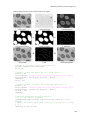
Rotate and Make Image Compact............................................................................... 266
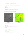
Edge Detection ........................................................................................................ 267
Apply Rainbow Palette to Gray Image ......................................................................... 269
Converting Image to Data ......................................................................................... 270
14 User Interaction ...............................................................................................271
14.1
Getting Numeric and String Input................................................................................... 271
14.1.1
14.1.2
14.1.3
14.2
Getting Points from Graph............................................................................................. 275
14.2.1
14.2.2
14.2.3
14.3
Get a Yes/No Response............................................................................................. 271
Get a String ............................................................................................................ 272
Get Multiple Values .................................................................................................. 272
Screen Reader ......................................................................................................... 275
Data Reader ............................................................................................................ 275
Data Selector .......................................................................................................... 277
Bringing Up a Dialog..................................................................................................... 279
15 Automation and Batch Processing ....................................................................283
15.1
15.2
15.3
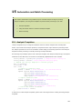
Analysis Templates....................................................................................................... 283
Using Set Column Values to Create an Analysis Template.................................................. 284
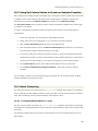
Batch Processing.......................................................................................................... 284
15.3.1
15.3.2
15.3.3
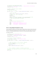
Processing Each Dataset in a Loop ............................................................................. 284
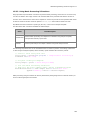
Using Analysis Template in a Loop ............................................................................. 285
Using Batch Processing X-Functions ........................................................................... 286
16 Reference Tables..............................................................................................287
16.1
16.2
Column Label Row Characters........................................................................................ 287
Date and Time Format Specifiers ................................................................................... 288
16.2.1
16.2.2
16.3
LabTalk Keywords ........................................................................................................ 290
16.3.1
16.3.2
16.4
16.5
16.6
16.7
16.8
Keywords in String................................................................................................... 290
Examples ................................................................................................................ 290
Last Used System Variables........................................................................................... 291
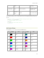
List of Colors ............................................................................................................... 293
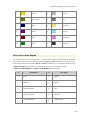
List of Line Styles......................................................................................................... 294
List of Symbol Shapes .................................................................................................. 296
System Variables ......................................................................................................... 297
16.8.1
16.8.2
16.8.3
16.9
Date Time Specifiers ................................................................................................ 288
Example ................................................................................................................. 290
Numeric System Variables ........................................................................................ 297
@ System Variables ................................................................................................. 299
Automatically Assigned System Variables.................................................................... 312
Text Label Options ....................................................................................................... 312
17 Function Reference ..........................................................................................315
17.1
LabTalk-Supported Functions......................................................................................... 315
17.1.1
17.1.2
17.1.3
17.1.4
17.2
Statistical Functions ................................................................................................. 315
Mathematical Functions ............................................................................................ 319
Origin Worksheet and Dataset Functions ..................................................................... 325
Notes on Use........................................................................................................... 331
LabTalk-Supported X-Functions ..................................................................................... 331
17.2.1
17.2.2
17.2.3
17.2.4
17.2.5
17.2.6
Data Exploration ...................................................................................................... 331
Data Manipulation .................................................................................................... 332
Database Access ...................................................................................................... 339
Fitting .................................................................................................................... 339
Graph Manipulation .................................................................................................. 340
Image .................................................................................................................... 342
vi
Table of Contents
17.2.7
17.2.8
17.2.9
17.2.10
17.2.11
17.2.12
Import and Export ................................................................................................... 345
Mathematics............................................................................................................ 348
Signal Processing ..................................................................................................... 350
Spectroscopy........................................................................................................... 352
Statistics ................................................................................................................ 352
Utility ..................................................................................................................... 354
Index......................................................................................................................361
vii
1
LabTalk Scripting Guide
In these pages we introduce LabTalk, the scripting language in Origin. LabTalk is designed for users who
wish to write and execute scripts to perform analysis and graphing of their data. The purpose of this
manual is to help users who are generally familiar with programming in a scripting language to take
advantage of the scripting capabilities in Origin. We provide sufficient detail for a user with basic
knowledge of Origin to begin tailoring the software to meet their unique needs.
New features are continually introduced to LabTalk with successive versions of Origin. Look for the version
number in which a feature was introduced in parentheses in or near the topic description (i.e., 8.1),
typically in a bold and/or red-colored font.
1
2
Introduction
Origin provides two programming languages: LabTalk and Origin C. This guide covers the LabTalk scripting
language. The guide is example based and provides numerous examples of accessing various aspects of
Origin from script.
The guide should be used in conjunction with the LabTalk Language Reference help file, which is accessible
from the Origin Help menu. The most up-to-date source of documentation including detailed examples can
be found at our wiki site: wiki.OriginLab.com
3
3
Getting Started with LabTalk
We begin with a classic example to show you how to execute LabTalk script.
3.1 Hello World
We demonstrate two ways to run your LabTalk scripts: (1) from the Script Window, (2) from the Custom
Routine toolbar button.
3.1.1
1.
Script Window
Open Origin, and from the Window pulldown menu, select the Script Window option. A new
window called Classic Script Window will open.
2.
In this new window, type the following text exactly and then press Enter:
type "Hello World"
You can execute LabTalk commands or functions line-by-line (or a selection of multiple
lines) to proceed through script execution step-by-step interactively. In script window,
press ENTER key to execute:
•
The current line if cursor has no selection.
•
The selected block if there is a selection.
Origin will output the text Hello World directly beneath your command.
3.1.2
Custom Routine
Origin provides a convenient way to save a script and run it with the push of a button.
1.
While holding down Ctrl+Shift on your keyboard, press the Custom Routine button (
) on
the Standard Toolbar.
2.
This opens Code Builder, Origin's native script editor. The file being edited is called
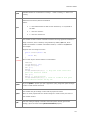
Custom.ogs. The code has one section, [Main], and contains one line of script:
[Main]
type -b $General.Userbutton;
3.
Replace that line with this one:
5
LabTalk Programming Guide for Origin 8.5.1
[Main]
type -b "Hello World";
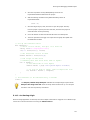
4.
And then select Save (
) in the Code Builder window.
5.
Now go back to the Origin project window and click
.
Origin will again output the text Hello World, but this time, because of the -b switch, to a pop-out window.
3.2 Hello LabTalk
Now that you are familiar with ways in which to write, save, and execute your LabTalk scripts, we can
begin using LabTalk to take advantage of the many other features of the Origin software. Again, we
provide simple examples for you to follow and get going quickly.
In the Classic Script Window type the following text exactly, and press Enter:
type -a "In %H, there are $(wks.ncols) columns."
Origin will output the following text in the same window, directly below your command:
In Book1, there are 2 columns.
%H is a String Register that holds the currently active window name (this could be a workbook, a matrix,
or a graph), while wks is a LabTalk Object that refers to the active worksheet; ncols is one attribute of
the wks object. The value of wks.ncols is then the number of columns in the active worksheet. The $ is
one of the substitution notations; it tells Origin to evaluate the expression that follows and return its
value.
3.3 Using = to Get Quick Output
The script window can be a calculator that returns result interactively. Type below script and press Enter:
3 + 5 =
Origin computes and types the result in the next line after equal sign:
3+5=8
The = character is typically used as an assignment, with a left hand side and a right hand side. When the
right hand side is missing, the interpreter will evaluate the expression on the left and print the result in
the script window.
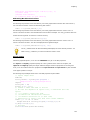
In the example below, we will introduce the concept of variables in LabTalk. Entering the following
assignment statement in the Script window:
A = 2
creates the variable A, and sets A equal to 2. Then you can do some arithmetic on variable A, like multiply
PI (a constant defined in Origin,
) and assign back to A
A = A*PI
To see the value of A:
6
Getting Started with LabTalk
A =
Press Enter and Origin responds with:
A=6.2831853071796
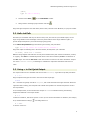
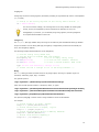
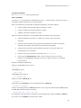
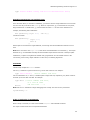
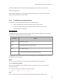
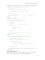
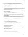
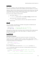
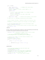
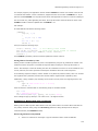
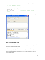
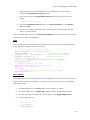
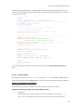
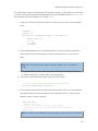
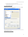
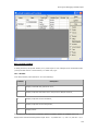
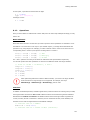
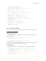
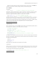
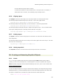
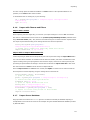
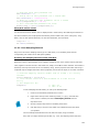
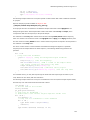
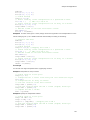
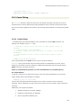
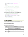
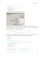
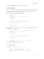
In addition, there are LabTalk Commands to view a list of variables and their values. Type list or edit and
press Enter:
list
Origin will open the LabTalk Variables and Functions dialog that lists all types of Origin variables as shown
below.
LabTalk supports various types of variables. See Data Types and Variables.
3.4 Working with Data
3.4.1
Input and Operators
Open a new Origin project. On a clean line of the Classic Script Window type the following text exactly
and press Enter:
Col(1) = {1:10}
In the above script, Col function is used to refer to the dataset in a worksheet column. Now look at the
worksheet in the Book1 window; the first 10 rows should contain the values 1--10. You have just created
a data series. So now you might want to do something with that series, say, multiply all of its values by a
constant. On another line of the Classic Script Window type
Col(2) = Col(1)*4
7
LabTalk Programming Guide for Origin 8.5.1
The first 10 rows of the second column of the worksheet in Book1 should now contain the values
corresponding to the first column, each multiplied by the constant 4.
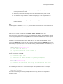
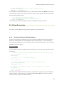
Origin also provides several built-in functions for generating data. For instance, the following code fills the
first 100 rows of column 2 (in the active worksheet) with uniformly distributed random numbers:
Col(2) = uniform(100)
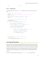
3.4.2
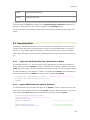
Import
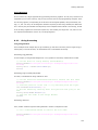
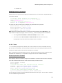
Most likely, you will want to do more than create simple data series; you will want to import data from
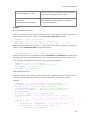
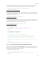
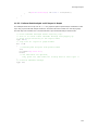
external applications and use Origin to plot and analyze that data. In LabTalk script, the easiest and best
way to do this is to use the impASC X-Function. For example:
// Specify the path to the desired data file.
string path$ = "D:\SampleData\Waveform.dat";
// Import the file into a new workbook (ImpMode = 3).
impasc fname:=path$ options.ImpMode:=3;
This example illustrates a script with more than one command. The path$ in the first line is a String
Variable that holds the file you want to import, then we pass this string variable as an argument to the
impASC X-Function. The semicolon at the end of each line tells Origin where a command ends. Two
forward-slash characters, //, tell Origin to treat the text afterward (until the end of the line) as a
comment. To run both of the commands above together, paste or type them into the Script Window,
select both lines (as you would a block of text to copy, they should be highlighted) and press enter. Origin
runs the entire selection (and ignores the comments).
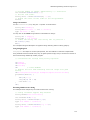
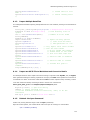
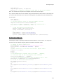
There are also many files containing sample data that come with your Origin installation. They are located
in the Samples folder under the path that you installed Origin locally (the system path). This example
accesses one such file:
string fn$=system.path.program$ +
"Samples\Spectroscopy\HiddenPeaks.dat";
// Start with a new worksheet (ImpMode = 4).
impasc fname:=fn$ options.ImpMode:=4;
The data tree named options stores all of the input parameters, which can be changed by direct access
as in the example.
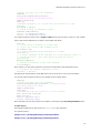
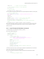
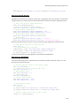
Once you have your data inside Origin, you will want a convenient way to access it from script. The best
way to do this is using the new Range Notation introduced in Origin 8:
// Assign your data of interest to a range variable.
range rr = [Book1]Sheet2!Col(4);
// Assign the range data to column 1 of the active worksheet.
Col(1) = rr;
// Change the value of the 4th element of the range to the value
10.
rr[4] = 10;
Although this example is trivial it shows off the power of range notation to access, move, and process your
data.
3.5 Where to Go from Here?
8
Getting Started with LabTalk
The answer to this question is the subject of the rest of the LabTalk Scripting Guide. The examples above
only scratch the surface, but have hopefully provided enough information for you to get a quick start and
excited you to learn more.
9
4
Language Fundamentals
This chapter covers the following topics:
1.
LT General Language Features
2.
LT Special Language Features
3.
LabTalk Script Precedence
In any programming language, there are general tasks that one will need to perform. They include:
importing, parsing, graphing, and exporting data; initializing, assigning, and deleting variables;
performing mathematical and textual operations on data and variables; imposing conditions on program
flow (i.e., if, if-else, break, continue); performing sets of tasks in a batch (e.g., macro) or in a loop
structure; calling and passing arguments to and from functions; and creating user-defined functions. Then
there are advanced tasks or functionalities specific to each language. This section demonstrates and
explains how to both carry out general programming tasks and utilize unique, advanced features in
LabTalk. In addition, we explain how to run LabTalk scripts within an Origin project.
4.1 General Language Features
These pages contain information on implementing general features of the LabTalk scripting language. You
will find these types of features in almost every programming language.
4.1.1
Data Types and Variables
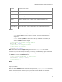
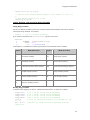
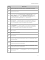
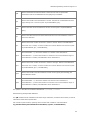
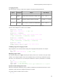
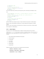
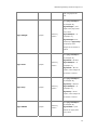
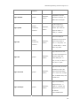
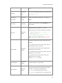
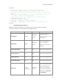
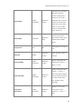
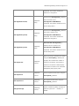
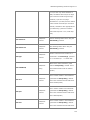
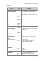
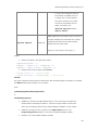
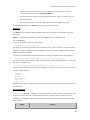
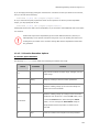
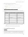
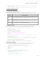
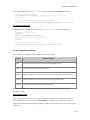
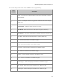
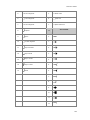
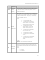
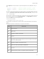
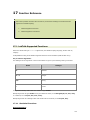
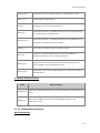
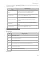
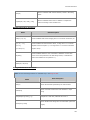
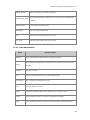
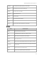
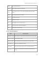
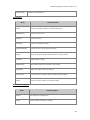
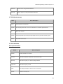
LabTalk Data Types
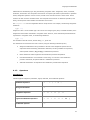
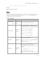
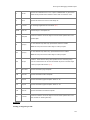
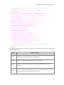
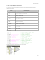
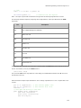
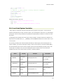
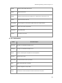
LabTalk supports 9 data types:
Type
Comment
Double
Double-precision floating-point number
Integer
Integers
Constant
Numeric data type that value cannot be changed once declared
11
LabTalk Programming Guide for Origin 8.5.1
Dataset
Array of numeric values
String
Sequences of characters
StringArray
Array of strings
Range
Refers to a specific region of Origin object (workbook, worksheet, etc.)
Tree
Emulates data with a set of branches and leaves
Graphic Object
Objects like labels, arrows, lines, and other user-created graphic elements
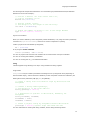
Numeric
LabTalk supports three numeric data types: double, int, and const.
1.
Double: double-precision floating-point number; this is the default variable type in Origin.
2.
Integer: integers (int) are stored as double in LabTalk; truncation is performed during
assignment.
3.
Constant: constants (const) are a third numeric data type in LabTalk. Once declared, the
value of a constant cannot be changed.
// Declare a new variable of type double:
double dd = 4.5678;
// Declare a new integer variable:
int vv = 10;
// Declare a new constant:
const em = 0.5772157;
Note: LabTalk does not have a complex datatype. You can use a complex number in a LabTalk
expression only in the case where you are adding or subtracting. LabTalk will simply ignore the imaginary
part and return only the real part. (The real part would be wrong in the case of multiplication or division.)
Use Origin C if you need the complex datatype.
// Only valid for addition or subtraction:
realresult = (3-13i) - (7+2i);
realresult=;
// realresult = -4
Dataset
The Dataset data type is designed to hold an array of numeric values.
Temporary Loose Dataset
When you declare a dataset variable it is stored internally as a local, temporary loose dataset. Temporary
means it will not be saved with the Origin project; loose means it is not affiliated with a particular
worksheet. Temporary loose datasets are used for computation only, and cannot be used for plotting.
12
Language Fundamentals
The following brief example demonstrates the use of this data type (Dataset Method and $ Substitution
Notation are used in this example):
// Declare a dataset 'aa' with values from 1-10,
// with an increment of 0.2:
dataset aa={1:0.2:10};
// Declare integer 'nSize',
// and assign to it the length of the new array:
int nSize = aa.GetSize();
// Output the number of values in 'aa' to the Script Window:
type "aa has $(nSize) values";
Project Level Loose Dataset
When you create a dataset by vector assignment (without declaration) or by using the Create (Command)
it becomes a project level loose dataset, which can be used for computation or plotting.
Create a project-level loose dataset by assignment,
bb = {10:2:100}
Or by using the Create command:
create %(strWks$) -wdn 10 aa bb;
For more on project-level and local-level variables see the section below on Scope of Variables.
For more on working with Datasets, see Datasets.
For more on working with %( ), see Substitution Notation.
String
LabTalk supports string handling in two ways: string variables and string registers.
String Variables
String variables may be created by declaration and assignment or by assignment alone (depending on
desired variable scope), and are denoted in LabTalk by a name comprised of continuous characters (see
Naming Rules below) followed by a $-sign (i.e., stringName$):
// Create a string with local/session scope by declaration and
assignment
// Creates a string named "greeting",
// and assigns to it the value "Hello":
string greeting$ = "Hello";
// $ termination is optional in declaration, mandatory for
assignment
string FirstName, LastName;
FirstName$ = Isaac;
LastName$ = Newton;
// Create a project string by assignment without declaration:
greeting2$ = "World";//global scope and saved with OPJ
For more information on working with string variables, see the String Processing section.
13
LabTalk Programming Guide for Origin 8.5.1
String Registers
Strings may be stored in String registers, denoted by a leading %-sign followed by a letter of the alphabet
(i.e., %A-%Z).
/* Assign to the string register %A the string "Hello World": */
%A = "Hello World";
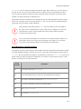
For current versions of Origin, we encourage the use of string variables for working with
strings, as they are supported by several useful built-in methods; for more, see
String(Object). If, however, you are already using string registers, see String Registers
for complete documentation on their use.
StringArray
The StringArray data type handles arrays of strings in the same way that the Datasets data type handles
arrays of numbers. Like the String data type, StringArray is supported by several built-in methods; for
more, see StringArray (Object).
The following example demonstrates the use of StringArray:
// Declare string array named "aa",
// and use built-in methods Add, and GetSize:
StringArray aa;
// aa is an empty string array
aa.Add("Boston");
// aa now has one element: "Boston"
aa.Add("New York");
// aa has a second element: "New York"
type "aa has $(aa.GetSize()) strings in it";
/* Prints "aa has 2 strings in it" in the Script Window. */
Range
The range data type allows functional access to any Origin object, referring to a specific region in a
workbook, worksheet, graph, layer, or window.
The general syntax is:
range rangeName = [WindowName]LayerNameOrIndex!DataRange
which can be made specific to data in a workbook, matrix, or graph:
range rangeName = [BookName]SheetNameOrIndex!ColumnNameOrIndex[RowBegin:RowEnd]
range rangeName = [MatrixBookName]MatrixSheetNameOrIndex!MatrixObjectNameOrIndex
range rangeName =[GraphName]LayerNameOrIndex!DataPlotIndex
The special syntax [??] is used to create a range variable to access a loose dataset.
For example:
// Access Column 3 on Book1, Sheet2:
range cc = [Book1]Sheet2!Col(3);
// Access second curve on Graph1, layer1:
range ll = [Graph1]Layer1!2;
// Access second matrix object on MBook1, MSheet1:
range mm = [MBook1]MSheet1!2;
// Access loose dataset tmpdata_a:
range xx = [??]!tmpdata_a;
14
Language Fundamentals
Notes:
•
CellRange can be a single cell, (part of) a row or column, a group of cells, or a
noncontiguous selection of cells.
•
Worksheets, Matrix Sheets and Graph Layers can each be referenced by name or index.
•
You can define a range variable to represent an origin object, or use range directly as an
X-Function argument.
•
Much more details on the range data type and uses of range variables can be found in
the Range Notation.
Tree
LabTalk supports the standard tree data type, which emulates a tree structure with a set of branches and
leaves. Branches contain leaves, and leaves contain data. Both branches and leaves are called nodes.
Leaf: A node that has no children, so it can contain a value
Branch: A node that has child nodes and does not contain a value
A leaf node may contain a variable that is of numeric, string, or dataset (vector) type.
Trees are commonly used in Origin to set and store parameters. For example, when a dataset is imported
into the Origin workspace, a tree called options holds the parameters which determine how the import is
performed.
Specifically, the following commands import ASCII data from a file called "SampleData.dat", and set
values in the options tree to control the way the import is handled. Setting the ImpMode leaf to a value
of 4 tells Origin to import the data to a new worksheet. Setting the NumCols leaf (on the Cols branch) to a
value of 3 tells Origin to only import the first three columns of the SampleData.dat file.
impasc fname:="SampleData.dat"
/* Start with new sheet */
options.ImpMode:=4
/* Only import the first three columns */
options.Cols.NumCols:=3
Declare a tree variable named aa:
// Declare an empty tree
tree aa;
// Tree nodes are added automatically during assignment:
aa.bb.cc=1;
aa.bb.dd$="some string";
// Declare a new tree 'trb' and assign to it data from tree 'aa':
tree trb = aa;
The tree data type is often used in X-Functions as a input and output data structure. For example:
// Put import file info into 'trInfo'.
impinfo t:=trInfo;
Tree nodes can be string. The following example shows how to copy treenode with string data to
worksheet column:
15
LabTalk Programming Guide for Origin 8.5.1
//Import the data file into worksheet
newbook;
string fn$=system.path.program$ +
"\samples\statistics\automobile.dat";
impasc fname:=fn$;
tree tr;
//Perform statistics on a column and save results to a tree
variable
discfreqs 2 rd:=tr;
// Assign strings to worksheet column.
newsheet name:=Result;
col(1) = tr.freqcount1.data1;
col(2) = tr.freqcount1.count1;
Tree nodes can also be vectors. Prior to Origin 8.1 SR1 the only way to access a vector in a Tree variable
was to make a direct assignment, as shown in the example code below:
tree tr;
// If you assign a dataset to a tree node,
// it will be a vector node automatically:
tr.a=data(1,10);
// A vector treenode can be assigned to a column:
col(1)=tr.a;
// A vector treenode can be assigned to a loose dataset, which is
// convenient since a tree node cannot be used for direct
calculations
dataset temp=tr.a;
// Perform calculation on the loose dataset:
col(2)=temp*2;
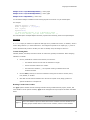
Now, however, you can access elements of a vector tree node directly, with statements such as:
// Following the example immediately above,
col(3)[1] = tr.a[3];
that assigns the third element of vector tr.a to the first row of column 3 in the current worksheet.
You can also output analysis results to a tree variable, like the example below.
newbook;
//Import the data file into worksheet
string fn$=system.path.program$ + "\samples\Signal
Processing\fftfilter1.dat";
impasc fname:=fn$;
tree mytr;
//Perform FFT and save results to a tree variable
fft1 ix:=col(2) rd:=mytr;
page.active=1;
col(3) = mytr.fft.real;
col(4) = mytr.fft.imag;
More information on trees can be found in the chapter on the Origin Project,Accessing Metadata section.
Graphic Objects
New LabTalk variable type to allow control of graphic objects in any book/layer.
The general syntax is:
GObject name = [GraphPageName]LayerIndex!ObjectName;
GObject name = [GraphPageName]LayerName!ObjectName;
16
Language Fundamentals
GObject name = LayerName!ObjectName; // active graph
GObject name = LayerIndex!ObjectName; // active graph
GObject name = ObjectName; // active layer
You can declare GObject variables for both existing objects as well as for not-yet created object.
For example:
GObject myLine = line1;
draw -n myLine -l {1,2,3,4};
win -t plot;
myLine.X+=2;
/* Even though myLine is in a different graph
that is not active, you can still control it! */
For a full description of Graphic Objects and their properties and methods, please see Graphic Objects.
Variables
A variable is simply an instance of a particular data type. Every variable has a name, or identifier, which is
used to assign data to it, or access data from it. The assignment operator is the equal sign (=), and it is
used to simultaneously create a variable (if it does not already exist) and assign a value to it.
Variable Naming Rules
Variable, dataset, command, and macro names are referred to generally as identifiers. When assigning
identifiers in LabTalk:
•
Use any combination of letters and numbers, but note that:
o
the identifier cannot be more than 25 characters in length.
o
the first character cannot be a number.
o
the underscore character "_" has a special meaning in dataset names and
should be avoided.
•
Use the Exist (Function) to check if an identifier is being used to name a window, macro,
tool, dataset, or variable.
•
Note that several common identifiers are reserved for system use by Origin, please see
System Variables for a complete list.
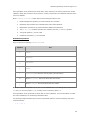
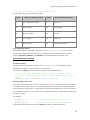
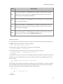
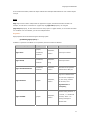
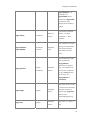
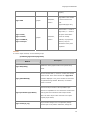
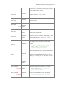
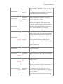
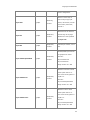
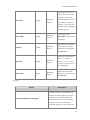
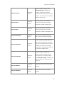
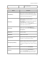
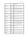
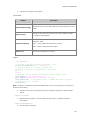
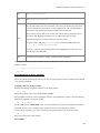
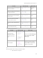
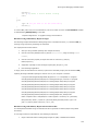
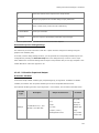
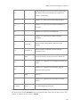
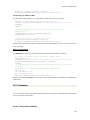
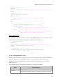
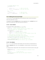
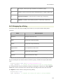
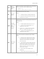
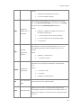
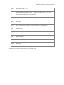
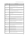
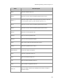
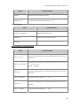
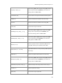
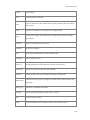
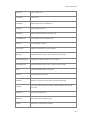
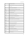
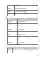
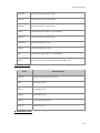
Handling Variable Name Conflicts
The @ppv system variable controls how Origin handles naming conflicts between project, session, and
local variables. Like all system variables, @ppv can be changed from script anytime and takes immediate
effect.
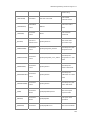
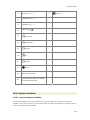
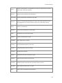
Variable
@ppv=0
Description
This is the DEFAULT option and allows both session variables and local variables to use
existing project variable names. In the event of a conflict, session or local variables
17
LabTalk Programming Guide for Origin 8.5.1
are used.
This option makes declaring a session variable with the same name as an existing
@ppv=1
project variable illegal. Upon loading a new project, session variables with a name
conflict will be disabled until the project is closed or the project variable with the same
name is deleted.
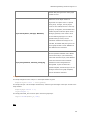
This option makes declaring a local variable with the same name as an existing project
@ppv=2
variable illegal. Upon loading of new project, local variables with a name conflict will be
disabled until the project is closed or the project variable with the same name is
deleted.
This is the combination of @ppv=1 and @ppv=2. In this case, all session and local
@ppv=3
variables will not be allowed to use project variable names. If a new project is loaded,
existing session or local variables of the same name will be disabled.
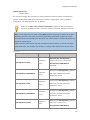
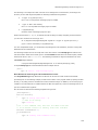
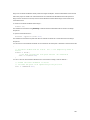
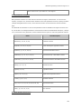
Listing and Deleting Variables
Use the LabTalk commands list and del for listing variables and deleting variables respectively.
/* Use the LabTalk command "list" with various options to list
variables; the list will print in the Script Window by default: */
list
list
list
list
a;
v;
vs;
vt;
//
//
//
//
List
List
List
List
all
all
all
all
the session
project and
project and
project and
variables
session variables
session string variables
session tree variables
// Use the LabTalk command "del" to delete variables:
del -al <variableName>;
variable
del -al *;
variables
// Delete specific local or session
// Delete all the local and session
// There is also a viewer for LabTalk variables:
// "ed" command can also open the viewer
list;
// Open the LabTalk Variables Viewer
Please see the List (Command), and Del (Command) (in Language Reference: Command Reference) for
all listing and deleting options.
If no options specified, List or Edit command will open the LabTalk Variables and Functions dialog to list all
variables and functions.
Scope of Variables
The scope of a variable determines which portions of the Origin project can see and be seen by that
variable. With the exception of the string, double (numeric), and dataset data types, LabTalk variables
must be declared. The way a variable is declared determines its scope. Variables created without
18
Language Fundamentals
declaration (double, string, and dataset only!) are assigned the Project/Global scope. Declared variables
are given Local or Session scope. Scope in LabTalk consists of three (nested) levels of visibility:
•
Project variables
•
Session variables
•
Local variables
Project (Global) Variables
•
Project variables , also called Global variables , are saved with the Origin Project (*.OPJ).
Project variables or Global variables are said to have Project scope or Global scope .
•
Project variables are automatically created without declarations for variables of type
double, string, and dataset as in:
// Define a project (global scope) variable of type double:
myvar = 3.5;
// Define a loose dataset (global scope):
temp = {1,2,3,4,5};
// Define a project (global scope) variable of type string:
str$ = "Hello";
•
All other variable types must be declared, which makes their default scope either Session
or Local. For these you can force Global scope using the @global system variable (below).
Session Variables
•
Session variables are not saved with the Origin Project, and are available in the current
Origin session across projects. Thus, once a session variable has been defined, they exist
until the Origin application is terminated or the variable is deleted.
•
When there are a session variable and a project variable of the same name, the session
variable takes precedence.
•
Session variables are defined with variable declarations, such as:
// Defines a variable of type double:
double var1 = 4.5;
// Define loose dataset:
dataset mytemp = {1,2,3,4,5};
It is possible to have a Project variable and a Session variable of the same name. In such a case, the
session variable takes precedence. See the script example below:
aa = 10;
type "First, aa is a project variable equal to $(aa)";
double aa = 20;
type "Then aa is a session variable equal to $(aa)";
del -al aa;
type "Now aa is project variable equal to $(aa)";
And the output is:
First, aa is a project variable equal to 10
Then aa is a session variable equal to 20
19
LabTalk Programming Guide for Origin 8.5.1
Now aa is project variable equal to 10
Local Variables
Local variables exist only within the current scope of a particular script.
Script-level scope exists for scripts:
•
enclosed in curly braces {},
•
in separate *.OGS files or individual sections of *.OGS files,
•
inside the Column/Matrix Values Dialog, or
•
behind a custom button (Button Script).
Local variables are declared and assigned value in the same way as session variables:
loop(i,1,10){
double a = 3.5;
const e = 2.718;
// some other lines of script...
}
// "a" and "e" exist only inside the code enclosed by {}
It is possible to have local variables with the same name as session variables or project variables. In this
case, the local variable takes precedence over the session or project variable of the same name, within
the scope of the script. For example, if you run the following script:
[Main]
double aa = 10;
type "In the main section, aa equals $(aa)";
run.section(, section1);
run.section(, section2);
[section1]
double aa = 20;
type "In section1, aa equals $(aa)";
[section2]
type "In Section 2, aa equals $(aa)";
Origin will output:
In the main section, aa equals 10
In section1, aa equals 20
In Section 2, aa equals 10
Forcing Global Scope
At times you may want to define variables or functions in a *.OGS file, but then be able to use them from
the Script Window (they would, by default, exist only while the *.OGS file was being run). To do so, you
need to use the @global system variable, which when given a value of 1, forces all variables to have
global or project level scope (its default value is 0). For Example:
[Main]
@global = 1;
// the following declarations become global
range a = 1, b= 2;
if(a[2] > 0)
{
20
Language Fundamentals
// begin a local scope
range c = 3; // this declaration is still global
}
Upon exiting the *.OGS, the @global variable is automatically restored to its default value, 0.
Note that one can also control a block of code by placing @global at the beginning and end such as:
@global=1;
double alpha=1.2;
double beta=2.3;
Function double myPeak(double x, double x0)
{
double y = 10*exp(-(x-x0)^2/4);
return y;
}
@global=0;
double gamma=3.45;
In the above case variables alpha, beta and the user-defined function myPeak will have global scope,
where as the variable gamma will not.
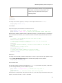
4.1.2
Programming Syntax
A LabTalk script is a single block of code that is received by the LabTalk interpreter. A LabTalk script is
composed of one or more complete programming statements, each of which performs an action.
Each statement in a script should end with a semicolon, which separates it from other statements.
However, single statements typed into the Script window for execution should not end with a semicolon.
Each statement in a script is composed of words. Words are any group of text separated by white space.
Text enclosed in parentheses is treated as a single word, regardless of white space. For example:
type This is a statement;
statement
ty s1; ty s2; ty s3;
// Single LabTalk
// Three statements
Parentheses are used to create long words containing white space. For example, in the script:
menu 3 (Long Menu Name);
the open parenthesis signifies the beginning of a single word, and the close parenthesis signifies the end
of the word.
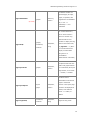
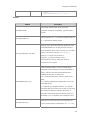
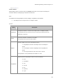
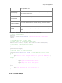
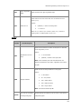
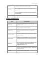
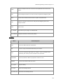
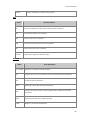
Statement Types
LabTalk supports five types of statements :
•
Assignment Statements
•
Macro Statements
•
Command Statements
•
Arithmetic Statement
•
Function Statements
21
LabTalk Programming Guide for Origin 8.5.1
Assignment Statements
The assignment statement takes the general form:
LHS = expression;
expression (RHS, right hand side) is evaluated and put into LHS (left hand side). If LHS does not exist, it
is created if possible, otherwise an error will be reported.
When a new data object is created with an assignment statement, the object created is:
•
A string variable if LHS ends with a $ as in stringVar$ = "Hello."
•
A numeric variable if expression evaluates to a scalar.
•
A dataset if expression evaluates to a range.
When new values are assigned to an existing data object, the following conventions apply:
•
If LHS is a dataset and expression is a scalar, every value in LHS is set equal to
expression.
•
If LHS is a numeric variable, then expression must evaluate into a scalar. If expression
evaludate into a dataset, LHS retrieves the first element of the dataset.
•
If both LHS and expression represent datasets, each value in LHS is set equal to the
corresponding value in expression.
•
If LHS is a string, then expression is assumed to be a string expression.
•
If the LHS is the object.property notation, with or without $ at the end, then this
notation is used to set object properties, such as the number of columns in a worksheet,
like wks.ncols=3;
Examples of Assignment Statements
Assign the variable B equal to the value 2.
B = 2;
Assign Test equal to 8.
Test = B^3;
Assign %A equal to Austin TX.
%A = Austin TX;
Assign every value in Book1_B to 4.
Book1_B = 4;
Assign each value in Book2_B to the corresponding position in Book1_B.
Book1_B = Book2_B;
Sets the row heading width for the Book1 worksheet to 100, using the worksheet object's rhw property.
The doc -uw command refreshes the window.
Book1!wks.rhw = 100;
doc -uw;
The calculation is carried out for the values at the corresponding index numbers in more and yetmore.
The result is put into myData at the same index number.
22
Language Fundamentals
myData = 3 * more + yetmore;
Note: If a string register to the left of the assignment operator is enclosed in parentheses, the string
register is substitution processed before assignment. For example:
%B = DataSet;
(%B) = 2 * %B;
The values in DataSet are multiplied by 2 and put back into DataSet. %B still holds the string "DataSet".
Similar to string registers, assignment statement is also used for string variables, like:
fname$=fdlg.path$+"test.csv";
In this case, the expression is a string expression which can be string literals, string variables, or
concatenation of multiple strings with the + character.
Macro Statements
Macros provide a way to alias a script, that is, to associate a given script with a specific name. This name
can then be used as a command that invokes the script.
For more information on macros, see Macros
Command Statements
The third statement type is the command statement. LabTalk offers commands to control or modify most
program functions.
Each command statement begins with the command itself, which is a unique identifier that can be
abbreviated to as little as two letters (as long as the abbreviation remains unique, which is true in most
cases). Most commands can take options (also known as switches), which are single letters that modify
the operation of the command. Options are always preceded by the dash "-" character. Commands can
also take arguments . Arguments are either a script or a data object. In many cases, options can also take
their own arguments.
Command statements take the general form:
command [option] [argument(s)];
The brackets [] indicate that the enclosed component is optional; not all commands take both options and
arguments. The brackets are not typed with the command statement (they merely denote an optional
component).
Methods (Object) are another form of command statement. They execute immediate actions relating to
the named object. Object method statements use the following syntax:
ObjectName.Method([options]);
For example:
The following script adds a column named new to the active worksheet and refreshes the window:
wks.addcol(new);
doc -uw;
The following examples illustrate different forms of command statements:
Integrate the dataset myData from zero.
integ myData;
23
LabTalk Programming Guide for Origin 8.5.1
Adding the -r option and its argument, baseline, causes myData to be integrated from a reference curve
named baseline.
integ -r baseline myData;
The repeat command takes two arguments to execute:
1.
the number of times to execute, and
2.
a script, which indicates the instruction to repeat.
This command statement prints "Hello World" in a dialog box three times.
repeat 3 {type -b "Hello World"}
Arithmetic Statement
The arithmetic statement takes the general form:
dataObject1 operator dataObject2;
where
•
dataObject1 is a dataset or a numeric variable.
•
dataObject2 is a dataset, variable, or a constant.
•
operator can be +, -, *, /, or ^.
The result of the calculation is put into dataObject1. Note that dataObject1 cannot be a function. For
example, col(3) + 25 is an illegal usage of this statement form.
The following examples illustrate different forms of arithmetic statements:
If myData is a dataset, this divides each value in myData by 10.
myData / 10;
Subtract otherData from myData, and put the result into myData. Both datasets must be Y or Z
datasets (see Note).
myData - otherData;
If A is a variable, increment A by 1. If A is a dataset, increment each value in A by 1.
A + 1;
Note: There is a difference between using datasets in arithmetic statements versus using datasets in
assignment statements. For example, data1_b + data2_b is computed quite differently from data1_b =
data1_b + data2_b. The latter case yields the true point-by-point sum without regard to the two
datasets' respective X-values. The former statement, data1_b + data2_b, adds the two data sets as if
each were a curve in the XY-plane. If therefore, data1_b and data2_b have different associated Xvalues, one of the two series will require interpolation. In this event, Origin interpolates based on the first
dataset's (data1_b in this case) X-values.
Function Statements
The function statement begins with the characteristics of a function -- an identifier -- followed by a
quantity, enclosed by parentheses, upon which the function acts.
An example of a function statement is:
24
Language Fundamentals
sum(dataset);
For more on functions in LabTalk, see Functions.
Using Semicolons in LabTalk
Separate Statements With Semicolon
Like the C programming language, LabTalk uses semicolons to separate statements. In general, every
statement should end with a semicolon. However, the following rules clarify semicolon usage:
•
Do not use a semicolon when executing a single statement script in the Script window.
o
An example of the proper syntax is:
type "hello" (ENTER).
o
The interpreter automatically places a semicolon after the statement to indicate
that it has been executed.
•
Statements ending with { } block can skip the semicolon.
•
The last statement in a { } block can also skip the semicolon.
In the following example, please note the differences between the three type command:
if (m>2) {type "hello";} else {type "goodbye"}
type "the end";
The above can also be written as:
if (m>2) {type "hello"} else {type "goodbye"}
type "the end";
or
if (m>2) {type "hello"} else {type "goodbye"};
type "the end";
Leading Semicolon for Delayed Execution
You can place a ';' in front of a script to delay its execution. This is often needed when you need to run a
script inside a button that will delete the button itself, like to issue window closing or new project
commands. For example, placing the following script inside a button will lead to problem (may crash)
// button to close this window
type "closing this window";
win -cn %H;
To fix this, the script should be written as
// button to close this window
type "closing this window";
;win -cn %H;
The leading ';' will place all scripts following it to be delayed-executed. Sometimes you may want a
specific group of statements delayed, then you can put them inside {script} with a leading ';', for
example:
// button to close this window
type "closing this window";
;{type "from delayed execution";win -cn %H;}
25
LabTalk Programming Guide for Origin 8.5.1
type "actual window closing code will be executed after this";
Extending a Statement over Multiple Lines
There are times when, for the sake of readability, you want to extend a single statement over more than
one line. One way to do this is with braces {}. When an "open brace", {, is encountered in a script file,
Origin searches for a "closed brace" , }, and executes the entire block of text as one statement. For
example, the following macro statement:
def openDialog {layer -s 1;
axis x;};
can also be written:
def openDialog {
layer -s 1;
axis x;
};
Both scripts are executed as a single statement, even though the second statement extends over four
lines.
Note: There is a limit to the length of script that can be included between a set of braces {}. The scripts
between the {} are translated internally and the translated scripts must be less than 1140 bytes (after
substitution). In place of long blocks of LabTalk code, programmers can use LabTalk macros or the
run.section() and run.file() object methods. To learn more, see Passing Arguments.
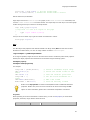
Comments
LabTalk script accepts two comment formats:
Use the "//" character to ignore all text from // to the end of the line. For example:
type "Hello World";
//Place comment text here.
Use the combination of "/*" and "*/" character pairs to begin and end, respectively, any block of code or
text that you do not want executed. For example:
type Hello /* Place comment text here,
or a line of code:
and even more ... */
World;
Note: Use the "#!" characters to begin debugging lines of script. The lines are only executed if
system.debug = 1.
Order of Evaluation in Statements
When a script is executed, it is sent to the LabTalk interpreter and evaluated as follows:
The script is broken down into its component statements
26
Language Fundamentals
Statements are identified by type using the following recognition order: assignment, macro, command,
arithmetic, and function. The interpreter first looks for an exposed (not hidden in parentheses or quotation
marks) assignment operator. If none is found, it looks to see if the first word is a macro name. It then
checks if the first word is a command name. The interpreter then looks for an arithmetic operation, and
finally, the interpreter checks whether the statement is a function.
The recognition order can have significant effect on script function. For example, the following assignment
statement:
type = 1;
assigns the value 1 to the variable type. This occurs even though type is (also) a LabTalk command, since
assignments come before commands in recognition order. However, since commands precede arithmetic
expressions in recognition order, in the following statement:
type + 1;
the command is carried out first, and the string, + 1, prints out.
The statements are executed in the order received, using the following evaluation priority
•
Assignment statements: String variables to the left of the assignment operator are not
expressed unless enclosed by parentheses. Otherwise, all string variables are expressed,
and all special notation ( %() and $()) is substitution processed.
•
Macro statements: Macro arguments are substitution processed and passed.
•
Command statements: If a command is a raw string, it is not sent to the substitution
processor. Otherwise, all special notation is substitution processed.
•
4.1.3
Arithmetic statements: All expressions are substitution processed and expressed.
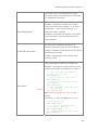
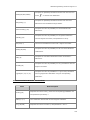
Operators
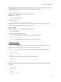
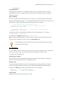
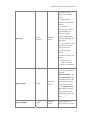
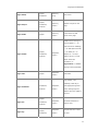
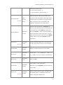
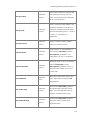
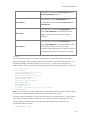
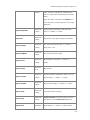
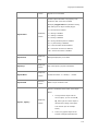
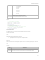
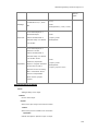
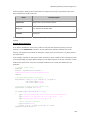
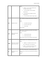
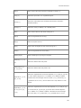
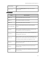
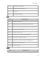
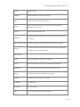
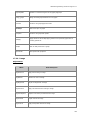
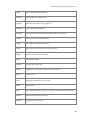
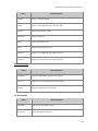
Introduction
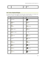
LabTalk supports assignment, arithmetic, logical, relational, and conditional operators:
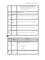
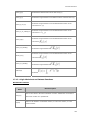
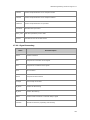
Arithmetic Operators
+
-
*
/
String Concatenation
+
Assignment Operators
=
+=
-=
Logical and Relational Operators
>
>=
<
Conditional Operator
?:
^
&
|
*=
/=
^=
<=
==
!=
&&
||
27
LabTalk Programming Guide for Origin 8.5.1
These operations can be performed on scalars and in many cases they can also be performed on vectors
(datasets). Origin also provides a variety of built-in numeric, trigonometric, and statistical functions which
can act on datasets.
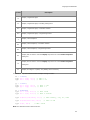
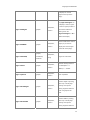
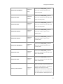
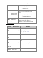
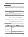
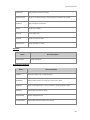
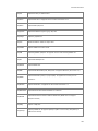
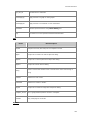
When evaluating an expression, Origin observes the following precedence rules:
1.
Exposed assignment operators (not within brackets) are evaluated.
2.
Operations within brackets are evaluated before those outside brackets.
3.
Multiplication and division are performed before addition and subtraction.
4.
The (>, >=, <, <=) relational operators are evaluated, then the (== and !=) operators.
5.
The logical operators || is prior to &&.
6.
Conditional expressions (?:) are evaluated.
Arithmetic Operators
Origin recognizes the following arithmetic operators:
Operator
Use
+
Addition
-
Subtraction
*
Multiplication
/
Division
^
Exponentiate (X^Y raises X to the Yth power) (see note below)
&
Bitwise And operator. Acts on the binary bits of a number.
|
Bitwise Or operator. Acts on the binary bits of a number.
Note: For 0 raised to the power n (0^n), if n > 0, 0 is returned. If n < 0, a missing value is returned. If n
= 0, then 1 is returned (if @ZZ = 1) or a missing value is returned (if @ZZ = 0).
These operations can be performed on scalars and on vectors (datasets). For more information on scalar
and vector calculations, see Performing Calculations below.
The following example illustrates the use of the exponentiate operator: Enter the following script in the
Command window:
1.3 ^ 4.7 =
28
Language Fundamentals
After pressing ENTER, 3.43189 is printed in the Command window. The next example illustrates the use of
the bitwise and operator: Enter the following script in the Command window:
if (27&41 == 9)
{type "Yes!"}
After pressing ENTER, Yes! is typed to the Command window.
Note: 27&41 == 9 because
27 = 0000000000011011
41 = 0000000000101001
with bitwise & yields:
0000000000001001 (which is equal to 9)
Note: Multiplication must be explicitly included in an expression (for example, 2*X rather than 2X to
indicate the multiplication of the variable X by the constant 2).
Define a constant
We can also define constant is defined in ORGSYS.CNF file as:
pi = 3.141592653589793
A Note about Logarithmic Conversion
•
To convert a dataset to a logarithmic scale, use the following syntax:
col(c) = log(col(c));
•
To convert a dataset back to a linear scale, use the following syntax:
col(c) = 10^(col(c));
String Concatenation
Very often you need to concatenate two or more strings of either the string variable or string register
type. All of the code segments in this section return the string "Hello World."
The string concatenation operator is the plus-sign (+), and can be used to concatenate two strings:
aa$ ="Hello";
bb$="World";
cc$=aa$+" "+bb$;
cc$=;
To concatenate two string registers, you can simply place them together:
%J="Hello";
%k="World";
%L=%J %k;
%L=;
If you need to work with both a string variable and a string register, follow these examples utilizing %( )
substitution:
aa$ ="Hello";
%K="World";
dd$=%(aa$) %K;
dd$=;
dd$=%K;
dd$=aa$+" "+dd$;
29
LabTalk Programming Guide for Origin 8.5.1
dd$=;
%M=%(aa$) %K;
%M=;
Assignment Operators
Origin recognizes the following assignment operators:
Operator
Use
Simple assignment.
=
+=
Addition assignment.
-=
Subtraction assignment.
*=
Multiplication assignment.
/=
Division assignment.
^=
Exponential assignment.
These operations can be performed on scalars and on vectors (datasets). For more information on scalar
and vector calculations, see Performing Calculations in this topic.
The following example illustrates the use of the -= operator.
In this example, 5 is subtracted from the value of A and the result is assigned to A:
A -= 5;
In the next example, each value in Data1_B is divided by the corresponding value in Book1_A, and the
resulting values are assigned to Book1_B.
Book1_B /= Book1_A;
In addition to these assignment operators, LabTalk also supports the increment and decrement operators
for scalar calculations (not vector).
Operator
++
--
Use
Add 1 to the variable contents and assign to the variable.
Subtract 1 from the variable contents and assign to the variable.
The following for loop expression illustrates a common use of the increment operator ++. The script types
the cell values in the second column of the current worksheet to the Command window:
30
Language Fundamentals
for (ii = 1; ii <= wks.maxrows; ii++)
{type ($(col(2)[ii])); }
Logical and Relational Operators
Origin recognizes the following logical and relational operators:
Operator
>
>=
<
Use
Greater than
Greater than or equal to
Less than
<=
Less than or equal to
==
Equal to
!=
Not equal to
&&
And
||
Or
An expression involving logical or relational operators evaluates to either true (non-zero) or false (zero).
Logical operators are almost always found in the context of Conditional and Loop Structures.
Numeric Comparison
The most common comparison is between two numeric values. Generally, at least one is a variable. For
instance:
if aa<3 type "aa<3";
Or, both items being compared can be variables:
if aa<=bb type "aa<=bb";
It is also possible, using parentheses, to make multiple comparisons in the same logical statement:
if (aa<3 && aa<bb) type "aa is lower";
String Comparison
You can use the == and != operators to compare two strings. String comparison (rather than numeric
comparison) is indicated by open and close double quotations (" ") either before, or after, the operator.
The following script determines if the %A string is empty:
if (%A == ""){type "empty"};
31
LabTalk Programming Guide for Origin 8.5.1
The following examples illustrates the use of the == operator:
x = 1;
// variable x is set to 1
%a = x;
// string a is set to "x"
if (%a == 1);
type "yes";
else
type "no";
The result will be yes, because Origin looks for the value of %a (the value of x), which is 1. In the
following script:
x = 1;
// variable x is set to 1
%a = x;
// string a is set to "x"
if ("%a" == 1)
type "yes";
else
type "no";
The result will be no, because Origin finds the quotation marks around %a, and therefore treats it as a
string, which has a character x, rather than the value 1.
Conditional Operator (?:)
The ternary operator or conditional operator (?:) can be used in the form:
Expression1 ? Expression2 : Expression3
This expression first evaluates Expression1. If Expression1 is true (non-zero), Expression2 is evaluated.
The value of Expression2 becomes the value for the conditional expression. If Expression1 is false (zero),
then Expression3 is evaluated and Expression3 becomes the value for the entire conditional expression.
Note that Expressions1 and Expressions2 can themselves be conditional operators. The following example
assigns the value which is greater (m or n), to variable:
m = 2;
n = 3;
variable = (m>n?m:n);
variable =
LabTalk returns: variable = 3
In this example, the script replaces all column A values between 5.5 and 5.9 with 5.6:
col(A) = col(A)>5.5&&col(A)<5.9?5.6:col(A);
Note: A Threshold Replace function treplace(dataset, value1, value2 [, condition]) is also available for
reviewing values in a dataset and replacing them with other values based on a condition. In the
treplace(dataset, value1, value2 [, condition]) function, each value in dataset is compared to value1
according to the condition. When the comparison is true, the value may be replaced with Value2 or Value2 depending on the value of condition. When the comparison is false, the value is retained or
replaced with a missing value depending on the value of condition. The treplace() function is much faster
than the ternary operator.
Performing Calculations
You can use LabTalk to perform both
32
Language Fundamentals
•
scalar calculations (mathematical operations on a single variable), and
•
vector calculations (mathematical operations on entire datasets).
Scalar Calculations
You can use LabTalk to express a calculation and store the result in a numeric variable. For example,
consider the following script:
inputVal = 21;
myResult = 4 * 32 * inputVal;
The second line of this example performs a calculation and creates the variable, myResult. The value of
the calculation is stored in myResult.
When a variable is used as an operand, and will store a result, shorthand notation can be used. For
example, the following script:
B = B * 3;
could also be written:
B *= 3;
In this example, multiplication is performed with the result assigned to the variable B. Similarly, you can
use +=, -=, /=, and ^=. Using shorthand notation produces script that executes faster.
Vector Calculations
In addition to performing calculations and storing the result in a variable (scalar calculation), you can use
LabTalk to perform calculations on entire datasets as well.
Vector calculations can be performed in one of two ways: (1) strictly row-by-row, or (2) using linear
interpolation.
Row-by-Row Calculations
Vector calculations are always performed row-by-row when you use the two general notations:
datasetB = scalarOrConstant <operator> datasetA;
datasetC = datasetA <operator> datasetB;
This is the case even if the datasets have different numbers of elements. Suppose there are three empty
columns in your worksheet: A, B and C. Run the following script:
col(a) = {1, 2, 3};
col(b) = {4, 5};
col(c) = col(a) + col(b);
The result in column C will be {5, 7, --}. That is, Origin outputs a missing value for rows in which one or
both datasets do not contain a value.
The vector calculation can also involve a scalar. In the above example, type:
col(c) = 2 * col(a);
Column A is multiplied by 2 and the results are put into the corresponding rows of column C.
Instead, execute the following script (assuming newData does not previously exist):
newData = 3 * Book1_A;
33
LabTalk Programming Guide for Origin 8.5.1
A temporary dataset called newData is created and assigned the result of the vector operation.
Calculations Using Interpolation
Origin supports interpolation through range notation and X-Functions such as interp1 and interp1xy.
Please refer to Interpolation for more details.
4.1.4
Conditional and Loop Structures
The structure of the LabTalk language is similar to C. LabTalk supports:
•
Loops, which allow the program to repetitively perform a set of actions.
•
Decision structures, which allow the program to perform different sets of actions
depending on the circumstances
Loop Structures
All LabTalk loops take a script as an argument. These scripts are executed repetitively under specified
circumstances. LabTalk provides four loop commands:
Command
Syntax
repeat
repeat value {script};
loop
loop (variable, startVal, endVal) {script};
doc -e
doc -e object {script};
for
for (expression1; expression2; expression3) {script};
The LabTalk for-loop is similar to the for loop in other languages. The repeat, loop, and doc -e loops are
less familiar, but are easy to use.
Repeat
The repeat loop is used when a set of actions must be repeated without any alterations.
Syntax: repeat value {script};
Execute script the number of times specified by value, or until an error occurs, or until the break
command is executed.
For example, the following script types the string three times:
repeat 3 { type "line of output"; };
Loop
The loop loop is used when a single variable is being incremented with each successive loop.
34
Language Fundamentals
Syntax: loop (variable, startVal, endVal) {script};
A simple increment loop structure. Initializes variable with a value of starVal. Executes script. Increments
variable and tests if it is greater than endVal. If it is not, executes script and continues to loop.
For example, the following script outputs numbers from 1 to 4:
loop (ii, 1, 4)
{type "$(ii)";};
Note: The loop command provides faster looping through a block of script than does the for command.
The enhanced speed is a result of not having to parse out a LabTalk expression for the condition required
to stop the loop.
Doc -e
The doc -e loop is used when a script is being executed to affect objects of a specific type, such as graph
windows. The doc -e loop tells Origin to execute the script for each instance of the specified object type.
Syntax: doc -e object {script};
The different object types are listed in the document command
For example, the following script prints the windows title of all graph windows in the project:
doc -e P {%H=}
For
The for loop is used for all other situations.
Syntax: for (expression1; expression2; expression3) {script};
In the for statement, expression1 is evaluated. This specifies initialization for the loop. Second,
expression2 is evaluated and if true (non-zero), the script is executed. Third, expression3, often
incrementing of a counter, is executed. The process repeats at the second step. The loop terminates when
expression2 is found to be false (zero). Any expression can consist of multiple statements, each separated
by a comma.
For example, the following script output numbers from 1 to 4:
for(ii=1; ii<=4; ii++)
{
type "$(ii)";
}
Note: The loop command provides faster looping through a block of script.
Decision Structures
Decision structures allow the program to perform different sets of actions depending on the
circumstances. LabTalk has three decision-making structures: if, if-else, and switch.
•
The if command is used when a script should be executed in a particular situation.
•
The if-else command is used when one script must be executed if a condition is true (nonzero), while another script is executed if the condition is false (zero).
•
The switch command is used when more than two possibilities are included in a script.
If, If-Else
35
LabTalk Programming Guide for Origin 8.5.1
Syntax:
1.
if (testCondition) sentence1; [else sentence2;]
2.
if (testCondition) {script1} [else {script2}]
Evaluate testCondition and if true, execute script1. Expressions without conditional operators are
considered true if the result of the expression is non-zero.
If the optional else is present and testCondition is false (zero), then execute script2. There should be a
space after the else. Strings should be quoted and string comparisons are not case sensitive.
Single statement script arguments should end with a semicolon. Multiple statement script arguments must
be surrounded by braces {}. Each statement within the braces should end with a semicolon. It is not
necessary to follow the final brace of a script with a semicolon.
For example, the following script opens a message box displaying "Yes!":
%M = test;
if (%M == "TEST") type -b "Yes!";
else type -b "No!";
The next script finds the first point in column A that is greater than -1.95:
newbook;
col(1)=data(-2,2,0.01);
val = -1.95;
get col(A) -e numpoints;
for(ii = 1 ; ii <= numpoints ; ii++)
{
// This will terminate the loop early if true
if (Col(A)[ii] > val) break;
}
if(ii > numpoints - 1)
ty -b No number exceeds $(val);
else
type -b The index number of first value > $(val) is $(ii)
The value is $(col(a)[ii]);
It is possible to test more than one condition with a single if statement, for instance:
if(a>1 && a<3) b+=1;
// If true, increment b by 1
The && (logical And) operator is one of several logical operators supported in LabTalk.
Switch
The switch command is used when more than two possibilities are included in a script. For example, the
following script returns b:
ii=2;
switch (ii)
{
case 1:
type "a";
break;
case 2:
type "b";
break;
case 3:
type "c";
36
Language Fundamentals
break;
default:
type "none";
break;
}
Break and Progress Bars
LabTalk provides a break command. When executed, this causes an exit from the loop and, optionally, the
script. This is often used with a decision structure inside a loop. It is used to protect against conditions
which would invalidate the loop test conditions. The break command can be used to display a progress
status dialog box (progress bar) to show the progress of looping.
Exit
The exit command prompts an exit from Origin unless a flag is set to restrict the exit.
Continue
The continue command can be used within the loop script. When executed, the remainder of the loop
script is ignored and the interpreter jumps to the next iteration of the loop. This is often used with a
decision structure inside a loop and can exclude illegal values from being processed by the loop script.
For example, in the following for loop, continue skips the type statement when ii is less than zero.
for (ii = -10; ii <= 10; ii += 2)
{
if (ii < 0)
continue;
type "$(sqrt(ii))";
}
Sections in a Script File
In addition to entering the script in the Label Control dialog, you can also save it as an Origin Script (OGS)
file. An Origin script file is an ASCII text file which consists of a series of one or more LabTalk statements.
Often, you can divide the statements into sections. A section is declared by a section name surrounded by
square brackets on its own line of text:
[SectionName]
Scripts under a section declaration belong to that section until another section declaration is met. A
framework for a script with sections will look like the following:
...
Scripts;
...
[Section 1]
...
Scripts;
...
[Section 2]
...
Scripts;
...
37
LabTalk Programming Guide for Origin 8.5.1
Scripts will be run in sequence until a new section flag is encountered, a return statement is executed or
an error occurs. To run a script in sections, you should use the
run.section(FileName, SectionName)
command. When filename is not included, the current running script file is assumed, for example:
run.section(, Init)
The following script illustrates how to call sections in an OGS file:
type "Hello, we will run section 2";
run.section(, section2);
[section1]
type "This is section 1, End the script.";
[section2]
type "This is section 2, run section 1.";
run.section(, section1);
To run the script, you can save it to your Origin user folder (Such as save as test.ogs), and type the
following in the command window:
run.section(test);
If code in a section could cause an error condition which would prematurely terminate a section, you can
use a variable to test for that case, as in:
[Test]
SectionPassed = 0;
// Here is where code that could fail can be run
...
SectionPassed = 1;
If the code failed, then SectionPassed will still have a value of 0. If the code succeeded, then
SectionPassed will have a value of 1.
4.1.5
Macros
Definition of the Macros
The command syntax,
define macroName {script}
defines a macro called macroName, and associates it with the given script. MacroName can then be used
like a command, and invokes the given script.
For example, the following script defines a macro that uses a loop to print a text string three times.
def hello
{
loop (ii, 1, 3)
{ type "$(ii). Hello World"; }
};
Once the hello macro is defined, typing the word hello in the Script window results in the printout:
38
Language Fundamentals
1. Hello World
2. Hello World
3. Hello World
Once a macro is defined, you can also see the script associated with it by typing
define macroName;
Passing Arguments to Macros
Macros can take up to five arguments. Use %1-%5 within the script for each argument. A macro can
accept a number, string, variable, dataset, function, or script as an argument. Passing arguments to a
macro is similar to passing arguments to a script.
If arguments are passed to a macro, the macro can report the number of arguments using the macro.nArg
object property.
For example, the following script defines a macro named double that expects a single numeric argument.
The given argument is then multiplied by 2, and the result is printed.
def double { type "$(%1 * 2)"; };
If you define this macro and then type the following in the Script window:
double 5
Origin outputs the result to the Script Window:
10
You could modify this macro to take two arguments:
def double { type "$(%1 * %2)"; };
Now, if you type the following in the Script window:
double 5 4
Origin outputs:
20
Macro Property
The macro object contains one property which, when inside a macro, contains the value for the number of
arguments.
Property
Macro.nArg
Access
Description
Read only,
Inside any macro, this property contains the value for the
numeric
number of arguments.
For example:
The following script defines a macro called TypeArgs. If three arguments are passed to the TypeArgs
macro, the macro types the three arguments to the Script window.
Def TypeArgs
{
if (macro.narg != 3)
{
39
LabTalk Programming Guide for Origin 8.5.1
type "Error! You must pass 3 arguments!";
}
else
{
type "The first argument passed was %1.";
type "The second argument passed was %2.";
type "The third argument passed was %3.";
}
};
If you define the TypeArgs macro as in the example, and then type the following in the Script window:
TypeArgs
One;
Origin returns the following to the Script window:
Error! You must pass 3 arguments!
If you define the TypeArgs macro as in the example, and then type the following in the Script window:
TypeArgs
One Two Three;
Origin returns the following to the Script window:
The first argument passed was One.
The second argument passed was Two.
The third argument passed was Three.
4.1.6
Functions
Functions are the core of almost every programming language; the following introduces function syntax
and use in LabTalk.
Built-In Functions
LabTalk supports many operations through built-in function s, a listing and description of each can be
found in Function Reference. Functions are called with the following syntax:
outputVariable = FunctionName(Arg1 Arg2 ... Arg N);
Below are a few examples of built-in functions in use.
The Count (Function) returns an integer count of the number of elements in a vector.
// Return the number of elements in Column A of the active
worksheet:
int cc = count(col(A));
The Ave (Function) performs a group average on a dataset, returning the result as a range variable.
range ra = [Book1]Sheet1!Col(A);
range rb = [Book1]Sheet1!Col(B);
// Return the group-averaged values:
rb = ave(ra, 5);
// 5 = group size
The Sin (Function) returns the sin of the input angle as type double (the units of the input angle are
determined by the value of system.math.angularunits):
system.math.angularunits=1;
double dd = sin(45);
// 1 = input in degrees
// ANS: DD = 0.7071
User-Defined Functions
40
Language Fundamentals
Support for multi-argument user-defined function s has been introduced in LabTalk for Origin 8.1. The
syntax for user-defined functions is:
function dataType funcName(Arg1 Arg2 ... ArgN) {script;}
Note:
1.
The function name should be less than 42 characters.
2.
Both arguments and return values support string, double, int, dataset and tree data types.
The default return type is int.
3.
By default, arguments of user-defined functions are passed by value, meaning that argument
values inside the function are NOT available outside of the function. However, passing arguments
by reference, in which changes in argument values inside the function WILL be available outside
of the function, is possible with the keyword REF.
Here are some simple cases of numeric functions:
// This function calculates the cube root of a number
function double dCubeRoot(double dVal)
{
double xVal;
if(dVal<0) xVal = -exp(ln(-dVal)/3);
else xVal = exp(ln(dVal)/3);
return xVal;
}
// As shown here
dcuberoot(-8)=;
The function below calculates the geometric mean of a dataset:
function double dGeoMean(dataset ds)
{
double dG = ds[1];
for(int ii = 2 ; ii <= ds.GetSize() ; ii++)
dG *= ds[ii]; // All values in dataset multiplied together
return exp(ln(dG)/ds.GetSize());
}
// Argument is anything returning a datset
dGeoMean(col("Raw Data"))=;
This example defines a function that accepts a range argument and returns the mean of the data in that
range:
// Calculate the mean of a range
function double dsmean(range ra)
{
stats ra;
return stats.mean;
}
// Pass a range that specifies all columns ...
// in the first sheet of the active book:
range rAll = 1!(1:end);
dsMean(rAll)=;
41
LabTalk Programming Guide for Origin 8.5.1
This example defines a function that counts the occurrences of a particular weekday in a Date dataset:
function int iCountDays(dataset ds, int iDay)
{
int iCount = 0;
for(int ii = 1 ; ii <= ds.GetSize() ; ii++)
{
if(weekday(ds[ii], 1) == iDay) iCount++;
}
return iCount;
}
// Here we count Fridays
iVal = iCountDays(col(1),6); // 6 is Friday in weekday(data, 1)
sense
iVal=;
Functions can also return datasets ..
// Get only negative values from a dataset
function dataset dsSub(dataset ds1)
{
dataset ds2;
int iRow = 1;
for(int ii = 1 ; ii <= ds1.GetSize() ; ii++)
{
if(ds1[ii] < 0)
{
ds2[iRow] = ds1[ii];
iRow++;
}
}
return ds2;
}
// Assign all negative values in column 1 to column 2
col(2) = dsSub(col(1));
or strings ..
// Get all values in a dataset where a substring occurs
function string strFind(dataset ds, string strVal)
{
string strTest, strResult;
for( int ii = 1 ; ii <= ds.GetSize() ; ii++ )
{
strTest$ = ds[ii]$;
if( strTest.Find(strVal$) > 0 )
{
strResult$ = %(strResult$)%(CRLF)%(strTest$);
}
}
return strResult$;
}
// Gather all instances in column 3 where "hadron" occurs
string MyResults$ = strFind(col(3),"hadron")$; // Note ending '$'
MyResults$=;
Passing Arguments by Reference
This example demonstrates a function that returns a tree node value as int (one element of a tree
variable). In addition, passing by reference is illustrated using the REF keyword.
42
Language Fundamentals
// Function definition:
Function int GetMinMax(range rr, ref double min, ref double max) {
stats rr;
//after running the stats XF, a LabTalk tree variable with the
//same name is created/updated
min = stats.min;
max = stats.max;
return stats.N;
}
// Call function GetMinMax to find min max for an entire worksheet:
double y1,y2;
int nn = getminmax(1:end,y1, y2);
type "Worksheet has $(nn) points, min=$(y1), max=$(y2)";
A more detailed example using tree variables in LabTalk functions and passing variables by reference, is
available in our online Wiki.
Another example of passing string argument by reference is given below that shows that the $ termination
should not be used in the function call:
//return range string of the 1st sheet
//actual new book shortname will be returned by Name$
Function string GetNewBook(int nSheets, ref string Name$)
{
newbook sheet:= nSheets result:=Name$;
string strRange$ = "[%(Name$)]1!";
return strRange$;
}
When calling the above function, it is very important that the Name$ argument should not have the $, as
shown below:
string strName$;
string strR$ = GetNewBook(1, strName)$;
strName$=;
strR$=;
Dataset Functions
Origin also supports defining mathematical functions that accept arguments of type double and return
type double. The general syntax for such functions is:
funcName(X) = expressionInvolvingX.
We call these dataset functions because when they are defined, a dataset by that name is created. This
dataset, associated with the function, is then saved as part of the Origin project. Once defined, a dataset
function can be referred to by name and used as you would a built-in LabTalk function.
For example, enter the following script in the Script window to define a function named Salary:
Salary(x) = 52 * x
Once defined, the function may be called anytime as in,
Salary(100)=
which yields the result Salary(100)=5200. In this case, the resulting dataset has only one element. But
if a vector (or dataset) were passed as an input argument, the output would be a dataset of the same
number of elements as the input.
43
LabTalk Programming Guide for Origin 8.5.1
As with other datasets, user-defined dataset functions are listed in dialogs such as Plot Setup (and can
be plotted like any other dataset), and in the Available Data list in dialogs such as Layer n.
If a 2D graph layer is the active layer when a function is defined, then a dataset of 100 points is created
using the X axis scale as the X range and the function dataset is automatically added to the plot layer.
The Function Graph Template (FUNCTION.OTP, accessible from the Standard Toolbar or the File: New
menu) also creates and plots dataset functions.
Origin's Function Plots feature allows new dataset functions to be easily created from any combination of
built-in and user-defined functions. In addition, the newly created function is immediately plotted for your
reference.
Access this feature in either of two ways:
1.
Click on the New Function button in the Standard toolbar,
2.
From the Origin drop-down menus, select File: New and select Function from the list of
choices, and click OK.
From there, in the Function tab of the Plot Details dialog that opens, enter the function definition, such
as, F1(x) = 5*sin(x)+1 and press OK. The function will be plotted in the graph.
You may define another function by clicking on the New Function button in the graph and adding another
function in Plot Details. Press OK, and the new function plot will be added to the graph. Repeat if more
functions are desired.
Fitting Functions
In addition to supporting many common functions, Origin also allows you to create your own fitting
functions to be used in non-linear curve fitting. User-defined fitting functions can also be used to generate
new datasets, but calling them requires a special syntax:
nlf_FitFuncName(ds, p1, p2, ... pn)
where the fitting function is named FitFuncName, ds is a dataset to be used as the independent variable,
and p1--pn are the parameters of the fitting function.
As a simple example, if you defined a simple straight-line fitting function called MyLine that expected a yintercept and slope as input parameters (in that order), and you wanted column C in the active worksheet
to be the independent variable (X), and column D to be used for the function output, enter:
// Intercept = 0, Slope = 4
Col(D) = nlf_MyLine(Col(C), 0, 4)
Scope of Functions
User-defined functions have a scope (like variables) that can be controlled. For more on scope see Data
Types and Variables. Please note that there are no project functions or global functions, that is different
from scope of variable.
44
Language Fundamentals
Similar to Session Variables, the scope of a function can be expanded for general use
throughout the current Origin session across projects by preceding the function definition
with the assignment @global=1.
You can associate functions with a project by defining them in the project's ProjectEvents.OGS file, using
the @Global=1 to promote them to session level.
To create a user-defined function for use across sessions, add commands in MACROS.CNF to run the
function definition .OGS files.
User-defined functions can be accessed from anywhere in the Origin project where LabTalk script is
supported, provided the scope of definition is applicable to such usage. Thus for example, a function
defined with preceding assignment @global=1 that returns type double or dataset, can be used in the
Set Values dialog Column Formula panel.
With preceding assignment @global=1, the function can be called anywhere.
[Main]
@global=1; // promote the following function to session
level
function double dGeoMean(dataset ds)
{
double dG = ds[1];
for(int ii = 2 ; ii <= ds.GetSize() ; ii++)
dG *= ds[ii]; // All values in dataset multiplied
together
return exp(ln(dG)/ds.GetSize());
}
// can call the function in [main] section
dGeoMean(col(1))=;
[section1]
// the function can be called in this section too
dGeoMean(col(1))=;
If the function is defined in a section of *.ogs file without @global=1, then it can only be called in its
own section.
[Main]
function double dGeoMean(dataset ds)
{
double dG = ds[1];
for(int ii = 2 ; ii <= ds.GetSize() ; ii++)
dG *= ds[ii]; // All values in dataset multiplied
together
return exp(ln(dG)/ds.GetSize());
}
// can call the function in [main] section
dGeoMean(col(1))=;
[section1]
// the function can NOT be called in this section
dGeoMean(col(1))=; // an error: Unknown function
If the function is defined in a block without @global=1, it can not be called outside this block.
[Main]
{ // define the function between braces
45
LabTalk Programming Guide for Origin 8.5.1
function double dGeoMean(dataset ds)
{
double dG = ds[1];
for(int ii = 2 ; ii <= ds.GetSize() ; ii++)
dG *= ds[ii]; // All values in dataset multiplied
together
return exp(ln(dG)/ds.GetSize());
}
}
// can Not call the function outside the braces
dGeoMean(col(1))=; // an error: Unknown function
Tutorial: Using Multiple Function Features
The following mini tutorial shows how to add a user-defined function at the Origin project level and then
use that function to create function plots.
1.
Start a new Project and use View: Code Builder menu item to open
Code Builder
2.
Expand the Project branch on the left panel tree and double-click to open
the ProjectEvents.OGS file. This file exists by default in any new Project.
3.
Under the [AfterOpenDoc] section, add the following lines of code:
@global=1;
Function double myPeak(double x, double x0)
{
double y = 10*exp(-(x-x0)^2/4);
return y;
}
4.
Save the file and close Code Builder
5.
In Origin, save the Project to a desired folder location. The OGS file is
saved with the Project, so the user-defined function is available for use in
the Project.
6.
Open the just saved project again. This will trigger the [AfterOpenDoc]
section to be executed and thus our myPeak function to be defined.
7.
Click on the New Function button in the Standard toolbar
8.
In the Function tab of Plot Details dialog that opens, enter the function
definition:
F1(x) = myPeak(x, 3)
and press OK. The function will be plotted in the graph.
9.
Click on the New Function button in the graph and add another function
in Plot Details using the expression:
F2(x) = myPeak(x, 4)
and press OK
46
Language Fundamentals
10. The 2nd function plot will be added to the graph
11. Now save the Project again and re-open it. The two function plots will still
be available, as they refer to the user-defined function saved with the
Project
12. You can assure yourself that the above really works by first exiting Origin,
reopening Origin, and running the project again, checking that the
myPeak function is defined upon loading the project.
4.2 Special Language Features
These pages contain information on implementing advanced features of the LabTalk scripting language.
Some of the concepts and features in this section are unique to Origin.
4.2.1
Range Notation
Introduction to Range
Inside your Origin Project, data exists in four primary places: in the columns of a worksheet, in a matrix,
in a loose dataset, or in a graph. In any of these forms, the range data type allows you to access your
data easily and in a standard way.
Once a range variable is created, you can work with the range data directly; reading and writing to the
range. Examples below demonstrate the creation and use of many types of range variables.
Before Origin Version 8.0, data were accessed via datasets as well as cell(), col() and wcol() functions.
The cell(), col() and wcol() functions are still very effective for data access, provided that you are working
with the active sheet in the active book. The Range notation essentially expanded upon these functions to
provide general access to any book, any sheet, or any plot inside the Origin Project.
Note : Not all X-Functions can handle complexities of ranges such as multiple columns or noncontiguous
data. Where logic or documentation does not indicate support, a little experimentation is in order.
Note : Data inside a graph are in the form of Data Plots and they are essentially references to columns,
matrix or loose datasets. There is no actual data stored in graphs.
Declaration and Syntax
Similar to other data types, you can declare a Range variable using the following syntax:
range [-option] RangeName = RangeString
The left-hand side of the range assignment is uniform for all types of range assignments. Note that the
square brackets indicate that the option switch is an optional parameter. At the present (8.1), option
47
LabTalk Programming Guide for Origin 8.5.1
switches only apply when assigning a range from a graph. Range names follow Origin variable naming
rules; please note that system variable names should be avoided.
The right-hand side of the range assignment, RangeString, changes depending on what type of object
the range points to. Individual Range Strings are defined in the sections below on Types of Range Data.
Range notation is used exclusively to define range variables. It cannot be used as a
general notation for data access on either side of an expression.
Accessing Origin Objects
A range variable can be assigned to the following types of Origin Objects:
•
column
•
worksheet
•
page
•
graph layer
•
loose dataset
Once assigned, the range will represent that object so that you can access the object properties and
methods using the range variable.
A range may consist of some subset or some combination of standard Origin Objects. Examples include:
•
column subrange
•
block of cells
•
XY range
•
XYZ range
•
composite range
Types of Range Data
Worksheet Data
For worksheet data, RangeString takes the form:
[WorkBookName]SheetNameOrIndex!ColumnNameOrIndex[CellIndex]
where ColumnName can be either the Long Name or the Short Name of the column.
In any RangeString, a span of continuous sheets, columns, or rows can be specified by providing pairs of
sheet, column, or row indices (respectively), separated by a colon, as in index1:index2. The keyword
end can replace index2 to indicate that Origin should pick up all of the indicated objects. For example:
range rs = [Book1]4:end!
range rd = [Book2]Sheet3!5:10;
// Get sheets 4 through last
// Get columns 5 through 10
In the case of rows the indices must be surrounded by square brackets, so a full range assignment
statement for several rows of a worksheet column looks like:
48
Language Fundamentals
range rc1 = [Book1]Sheet2!Col(3)[10:end];
last
range rc2 = [Book1]Sheet2!Col(3)[10:20];
20
// Get rows 10 through
// Get rows 10 through
The old way of accessing cell contents, via the Cell function is still supported.
If you wish to access column label rows using range, please see Accessing Metadata and the Column Label
Row Reference Table.
Column
When declaring range variable for a column on the active worksheet, the book and sheet part can be
dropped, such as:
range rc = Col(3)
You can further simplify the notation, as long as the actual column can be identified, as shown below:
range aa=1;
// col(1) of the active worksheet
range bb=B;
// col(B) of the active worksheet
range cc="Test A"; // col with Long Name ("Test A"), active
worksheet
Multiple range variables can be declared on the same line, separated by comma. The above example could
also have been written as:
range aa = 1, bb = B, cc = "Test A";
Or if you need to refer to a different book sheet, and all in the same sheet, then the book sheet portion
can be combined as follows:
range [Book2]Sheet3 aa=1, bb=B, cc="Test A";
Because Origin does not force a column's Long Name to be unique (i.e., multiple columns in a worksheet
can have the same Long Name), the Short Name and Long Name may be specified together to be more
precise:
range dd = D"Test 4";
range
// Assign Col(D), Long Name 'Test 4', to a
Once you have a column range, use it to access and change the parameters of a column:
range rColumn = [Book1]1!2;
rColumn.digitMode = 1;
display
rColumn.digits = 2;
// Range is a Column
// Use Set Decimal Places for
// Use 2 decimal places
Or perform computations:
// Point to column 1 of sheets 1, 2 and 3 of the active workbook:
range aa = 1!col(1);
range bb = 2!col(1);
range cc = 3!col(1);
cc = aa+bb;
When performing arithmetic on data in different sheets, you need to use range variables.
Direct references to range strings are not yet supported. For example, the script
Sheet3!col(1) = Sheet1!col(1) + Sheet2!col(1); will not work! If you really need to
write in a single line without having to declare range variables, then another alternative is
49
LabTalk Programming Guide for Origin 8.5.1
to use Dataset Substitution
Page and Sheet
Besides a single column of data, range can be used to access any portion of a page object:
Use a range variable to access an entire workbook:
// 'rPage' points to the workbook named 'Book1'
range rPage = [Book1];
// Set the Long Name of 'Book1' to "My Analysis Worksheets"
rPage.LongName$ = My Analysis Worksheets;
Use a range variable to access a worksheet:
range rSheet = [Book1]Sheet1!;
object)
rSheet.name$ = "Statistics";
"Statistics".
rSheet.AddCol(StdDev);
// Range is a Worksheet (WKS
// Rename Sheet1 to
// Add a column named StdDev
Column Subrange
Use a range variable to address a column subrange, such as
// A subrange of col(a) in book1 sheet2
range cc = [book1]sheet2!col(a)[3:10];
Or if the desired workbook and worksheet are active, the shortened notation can be used:
// A subrange of col(a) in book1 sheet2
range cc = col(a)[3:10];
Use range variables, you can perform computation or other operations on part of a column. For example:
range r1=1[5:10];
range r2=2[1:6];
r1 = r2; // copy values in row 1 to 6 of column 2 to rows 5 to 10
of column 1
r1[1]=;
// this should output value in row 5 of column 1, which equates to
row 1 of column 2
Block of Cells
Use a range to access a single cell or block of cells (may span many rows and columns) as in:
range aa = 1[2];
range bb = 1[1]:3[10];
// cell(2,1), row2 of col(1)
// cell(1,1) to cell(10,3)
Note: a range variable representing a block of cells can be used as an X-Function argument only, direct
calculations are not supported.
Matrix Data
For matrix data, the RangeString is
[MatrixBookName]MatrixSheetNameOrIndex!MatrixObject
Make an assignment such as:
50
Language Fundamentals
// Second matrix object on MBook1, MSheet1
range mm = [MBook1]MSheet1!2;
Access the cell contents of a matrix range using the notation RangeName[row, col]. For example:
range mm=[MBook1]1!1;
mm[2,3]=10;
If the matrix contains complex numbers, the string representing the complex number can be accessed as
below:
string str$;
str$ = mm[3,4]$;
Graph Data
For graph data, the RangeString is
[GraphWindowName]LayerNameOrIndex!DataPlot
An example assignment looks like
range ll = [Graph1]Layer1!2;
Layer1
// Second curve on Graph1,
Option Switches -w and -wx
For graph windows, you can use the range -w and range -wx options to get the worksheet column range
of a plotted dataset.
// Make a graph window the active window ...
// Get the worksheet range of the Y values of first dataplot:
range -w rW = 1;
// Get the worksheet range of the corresponding X-values:
range -wx rWx = 1;
// Get the graph range of the first dataplot:
range rG = 1;
// Get the current selection (%C); will resolve data between
markers.
range -w rC = %C;
Note that in the script above, rW = [Book1]Sheet1!B while rG = [Graph1]1!1.
Data Selector Ranges on a Graph
You can use the Data Selector tool to select one or more ranges on a graph and to refer to them from
LabTalk. For a single selected range, you can use the MKS1, MKS2 system variables. Starting with version
8.0 SR6, a new X-Function, get_plot_sel, has been added to get the selected ranges into a string that
you can then parse. The following example shows how to select each range on the current graph:
string strRange;
get_plot_sel str:=strRange;
StringArray sa;
sa.Append(strRange$,"|"); // Tokenize it
int nNumRanges = sa.GetSize();
if(nNumRanges == 0)
{
51
LabTalk Programming Guide for Origin 8.5.1
type "there is nothing selected";
return;
}
type "Total of $(nNumRanges) ranges selected for %C";
for(int ii = 1; ii <= nNumRanges; ii++)
{
range -w xy = sa.GetAt(ii)$;
string strWks$ = "Temp$(ii)";
create %(strWks$) -wdn 10 aa bb;
range fitxy = [??]!(%(strWks$)_aa, %(strWks$)_bb);
fitlr iy:=xy oy:=fitxy;
plotxy fitxy p:=200 o:=<active> c:=color(red) rescale:=0
legend:=0;
type "%(xy) fit linear gives slope=$(fitlr.b)";
}
// clear all the data markers when done
mark -r;
Additional documentation is available for the the Create (Command) (for creating loose datasets), the [??]
range notation (for creating a range from a loose dataset), the fitlr X-Function, and the StringArray
(Object) (specifically, the Append method, new to Origin 8.0 SR6).
Loose Dataset
Loose Datasets are similar to columns in a worksheet but they don't have the overhead of the book-sheetcolumn organization. They are typically created with the create command, or automatically created from
an assignment statement without Dataset declaration.
The RangeString for a loose dataset is:
[??]!LooseDatasetName
An example assignment looks like this:
range xx = [??]!tmpdata_a;
// Loose dataset 'tmpdata_a'
To show how this works, we use the plotxy X-Function to plot a graph of a loose dataset.
// Create 2 loose datasets
create tmpdata -wd 50 a b;
tmpdata_a=data(50,1,-1);
tmpdata_b=normal(50);
// Declare the range and explicitly point to the loose dataset
range aa=[??]!(tmpdata_a, tmpdata_b);
// Make a scatter graph with it:
plotxy aa;
Please read more about Using Ranges in X-Functions.
Loose datasets belong to a project, so they are different from a Dataset variable, which is
declared, and has either session or local scope. Dataset variables are also internally loose
datasets but they are limited to use in calculations only; they cannot be used in making
plots, for example.
Unique Uses of Range
Manipulating Range Data
52
Language Fundamentals
A column range can be used to manipulate data directly. One major advantage of using a range rather
than the direct column name, is that you do not need to be concerned with which page or layer is active.
For example:
// Declare two range variables, v1 and v2:
range [Book1]Sheet1 r1=Col(A), r2=Col(B);
// Same as col(A)=data(1,30) if [book1]sheet1 is active:
r1 = data(1,30);
r2 = uniform(30);
// Plot creates new window so [Book1]Sheet1 is NOT active:
plotxy 2;
sec -p 1.5;
// Delay
r2/=4;
// But our range still works; col(A)/=4 does
NOT!
sec -p 1.5;
// Delay
r2+=.4;
sec -p 1.5;
// Delay
r1=10+r1/3;
Direct calculations on a column range variable that addresses a range of cells is supported. For example:
range aa = Col(A)[10:19]; // Row 10 to 19 of column A
aa += 10;
// All elements in aa increase by 10
Support for sub ranges in a column has expanded.
// Range consisting of column 1, rows 7 to 13 and column 2, rows 3
to 4
// Note use of parentheses and comma separator:
range rs = (1[7:13], 2[3:4]);
del rs; // Supported since 8.0 SR6
// Copying between sub ranges
range r1 = 1[85:100];
range r2 = 2;
// Copy r1 to top of column 2
r2 = r1; // Supported in 8.1
// 8.1 also complete or incomplete copying to sub range
range r2 = 2[17:22];
r2 = r1; // Only copies 6 values from r1
range r2 = 3[50:200];
r2 = r1; // Copies only up to row 65 since source has only 16
values
Dynamic Range Assignment
Sometimes it is beneficial to be able to create a new range in an automated way, at runtime, using a
variable column number, or the name of another range variable.
Define a New Range Using an Expression for Column Index
The wcol() function is used to allow runtime resolution of actual column index, as in
int nn = 2;
range aa=wcol(2*nn +1);
Define a New Range Using an Existing Range
53
LabTalk Programming Guide for Origin 8.5.1
The following lines of script demonstrate how to create one range based on another using the %( )
substitution notation and wks (object) methods. When the %( ) substitution is used on a range variable,
it always resolves it into a [Book]Sheet! string, regardless of the type:
range rwks = sheet3!;
range r1= %(rwks)col(a);
in this case, the new range r1 will resolve to Sheet3!Col(A).
This method of constructing new range based on existing range is very useful because it allows code
centralization to first declare a worksheet range and then to use it to declare column ranges. Lets now use
the rwks variable to add a column to Sheet 3:
rwks.addcol();
And now define another range that resolves to the last (rightmost) column of range rwks; that is, it will
point to the newly made column:
range r2 = %(rwks)wcol( %(rwks)!wks.ncols );
With the range assignments in place it is easy to perform calculations and assignments, such as:
r2=r1/10;
which divides the data in range r1 by 10 and places the result in the column associated with range r2.
X-Function Argument
Many X-functions use ranges as arguments. For example, the stats X-Function takes vector as input and
calculates descriptive statistics on the specified range. So you can type:
stats [Book1]Sheet2!(1:end); // stats on the second sheet of book1
stats Col(2);
// stats on column 2 of active
worksheet
// stats on block of cells, col 1-2, row 5-10
stats 1[5]:2[10];
Or you can use a range variable to do the same type of operation:
/* Defines a range variable for col(2) of 1st and 2nd sheet,
rows 3-5, and runs the stats XF on that range: */
range aa = (1,2)!col(2)[3:5]; stats aa;
The input vector argument for this X-Function is then specified by a range variable
Some X-Functions use a special type of range called XYRange, which is essentially a composite range
containing X and Y as well as error bar ranges.
The general syntax for an XYRange is
(rangeX, rangeY)
but you can also skip the rangeX portion and use the standard range notation to specify an XYRange, in
which case the default X data is assumed.
The following two notations are identical for XYRange,
(, rangeY)
rangeY
For example, the integ1 X-Function takes both input and output XYRange,
// integrate col(1) as X and col(2) as Y,
// and put integral curve into columns 3 as X and 4 as Y
54
Language Fundamentals
integ1 iy:=(1,2) oy:=(3,4);
// same as above except result integral curve output to col(3) as
Y,
// and sharing input's X of col(1):
integ1 iy:=2 oy:=3;
Listing, Deleting, and Converting Range Variables
Listing Range Variables
Use the list LabTalk command to print a list of names and their defined bodies of all session variables
including the range variables. For example:
list a; // List all session variables
If you issue this command in the Command Window, it prints a list such as:
Session:
1
MYRANGE
2
MYSTR
3
PI
[book1]sheet1!col(b)
"abc"
3.1415926535898
As of Origin 8.1, we added more switches (given below) to list particular session variables:
Option
What Gets Listed
Option
What Gets Listed
a
All session variables
aa
String arrays (session)
ac
Constants (session)
af
Local Function (session)
afc
Local Function Full Content (session)
afp
Local Function Prototype (session)
ag
Graphic objects (session)
ar
Range variables (session)
as
String variables (session)
at
Tree variables (session)
av
Numeric variables (session)
--
--
Deleting Range Variables
To delete a range variable, use the del LabTalk command with the -ra switch. For example:
range aa=1;
range ab=2;
range ac=3;
range bb=4;
list a;
ac, bb
del -ra a*;
letter "a"
//
//
//
//
//
aa =
ab =
ac =
bb =
list
Col(1) of the active worksheet
Col(2) of the active worksheet
Col(3) of the active worksheet
Col(4) of the active worksheet
all session variables; will include aa, ab,
// delete all range variables beginning with the
55
LabTalk Programming Guide for Origin 8.5.1
// The last command will delete aa, ab, and ac.
The table below lists options for deleting variables
Option
What Gets Deleted/Cleared
Option
What Gets Deleted/Cleared
ra
Any Local/Session variable
al
same as -ra
rar
Range variable
ras
String variable
rav
Numeric variable
rac
Constant
rat
Tree variable
raa
String array
rag
Graphic object
raf
Local/Session Function
Converting Range to UID
Each Origin Object has a short name, a long name, and a universal identifier (UID). You can convert
between range variables and their UIDs as well as obtain the names of pages and layers using the
functions range2uid, uid2name, and uid2range. See LabTalk Objects for examples of use.
Special Notations for Range
XY and XYZ Range
Designed as inputs to particular X-Functions, an XY Range (XYZ Range) is an ordered pair (triple)
designating two (three) worksheet columns as XY (XYZ) data.
For instance, the fitpoly X-Function takes an XY range for both input and output:
// Fit a 2nd order polynomial to the XY data in columns 1 and 2;
// Put the coefficients into column 3 and the XY fit data in cols 4
and 5:
fitpoly iy:=(1,2) polyorder:=2 coef:=3 oy:=(4,5);
XY Range using # and ? for X
There are two special characters '?' and '#' introduced in (8.0 SR3) for range as an X-Function argument.
'?' indicates that the range is forced to use worksheet designation, and will fail if the range designation
does not satisfy the requirement. '#' means that the range ignores designations and uses row number as
the X designation. However, if the Y column has even sampling information, that sampling information will
be used to provide X.
For example:
plotxy (?, 5);
fails
plotxy (#, 3);
// if col(5) happens to be X column call
// plot col(3) as Y and use row number as X
These notations are particularly handy in the plotxy X-Function, as demonstrated here:
56
Language Fundamentals
// Plot all columns in worksheet using their column designations:
plotxy (?,1:end);
Tag Notations in Range Output
Many X-Functions have an output range that can be modified with tags, including template, name and
index. Here is an example that can be used by the Discrete Frequency X-Function, discfreqs
discfreqs irng:=1 freq:=1 rd:="[Result]<new template:=table.otw
index:=3>";
The output is directed to a Workbook named Result by loading a template named TABLE.OTW as the third
sheet in the Result book.
Support of these tag notations depends on the particular X-Function, so experiment before including in
production code.
Composite Range
A Composite Range is a range consisting of multiple subranges. You can construct composite ranges using
the following syntax:
// Basic combination of three ranges:
(range1, range2, range3)
// Common column ranges from multiple sheets:
(sheet1,sheet2,sheet3)!range1
// Common column ranges from a range of sheets
(sheet1:sheetn)!range1
To show how this works, we will use the wcellcolor X-Function to show range and plotxy to show
XYRange. Assume we are working on the active book/sheet, with at least four columns filled with numeric
data:
// color several different blocks with blue color
wcellcolor (1[1]:2[3], 1[5]:2[5], 2[7]) color(blue);
// set font color as red on some of them
wcellcolor (1[3]:4[5], 2[6]:3[7]) color(red) font;
To try plotxy, we will put some numbers into the first sheet, add a new sheet, and put more numbers into
the second sheet.
// plot A(X)B(Y) from both sheets into the same graph.
plotxy (1:2)!(1,2);
// Activate workbook again and add more sheets and fill them with
data.
// Plot A(X)B(Y) from all sheets between row2 and row10:
plotxy (1:end)!(1,2)[2:10];
Note: There exists an inherent ambiguity between a composite range, composed of ranges r1 and r2 as
in (r1,r2), and an XY range composed of columns named r1 and r2, i.e., (r1,r2). Therefore, it is
important that one keep in mind what type of object is assigned to a given range variable!
4.2.2
Substitution Notation
57
LabTalk Programming Guide for Origin 8.5.1
Introduction
When a script is executed, it is sent to the LabTalk interpreter. Among other tasks, the interpreter
searches for special substitution notations which are identified by their initial characters, % or $. When a
substitution notation is found, the interpreter replaces the original string with another string, as described
in the following section. The value of the substituted string is unknown until the statement is actually
executed. Thus, this procedure is called a run-time string substitution.
There are three types of substitutions described below:
•
String register substitution, %A - %Z
•
%( ) Substitution, a powerful notation to resolve %(str), %(range), worksheet info and
column dataset names, worksheet cells, legend and etc.
•
$( ) Substitution, where $(expression) resolves the numeric expression and formats the
result as a string
%A - %Z
Using a string register is the simplest form of substitution. String registers are substituted by their
contents during script execution, for example
FDLOG.Open(A);
%B=FDLOG.path$;
doc -open %B%A;
// put file name into %A from dialog
// file path put into %B
// %B%A forms the full path file name
String registers are used more often in older scripts, before the introduction of string variables (Origin 8),
which allows for more reliable codes. To resolve string variables, %( ) substitution is used, and is
discussed in the next section.
%( ) Substitution
String Expression Substitution
While LabTalk commands often accept numeric expressions as arguments, none accept a string
expression. So if a string is needed as an argument, you have to pass in a string variable or a string
expression using the %( ) substitution to resolve run-time values. The simplest form of a string expression
is a single string variable, like in the example below:
string str$ = "Book2";
win -o %(str$) {wks.ncols=;}
Keyword Substitution
The %( ) substitution notation is also used to insert non-printing characters (also called control
characters), such as tabs or carriage returns into strings. Use LabTalk keywords to access these nonprinting characters. For example,
// Insert a carriage-return, line-feed (CRLF) into a string:
string ss$ = "Hello%(CRLF)Goodbye";
ss$=;
// ANS: 'Hello', 'Goodbye' printed on separate lines
// Or use %() substitution to display the string variable:
58
Language Fundamentals
type %(ss$);
Worksheet Column and Cell Substitution
The following notation allows you to access worksheet cells as a string as well as to get column dataset
name from any book sheet. Before Origin 8, each book had only one sheet so you could refer to its
content with the book name only. Since Origin 8 supports multiple worksheets, we recommend that you
use [workbookname]sheetname to address a specific sheet, unless you are certain that the book has
only one sheet.
To return individual cell contents, use the following syntax:
•
This notation references the active sheet in the named book
%(workbookName, column, row)
•
New Origin 8 notation that specifies book and sheet
%([workbookname]sheetname, column, row[,format])
For example, if the third cell in the fourth column in the active worksheet of Book1 contains the value 25,
then entering the following statement in the Script window will set A to 25 and put double that value in
another sheet in Book1.
A = %(Book1, 4, 3);
%([Book1]Results, 1, 4) = 2 * A;
To return the contents of a text cell, use a string variable:
string strVar$ = %(Book1, 2, 5); // Note : No end '$' needed here
strVar$ = ;
Before 8.1, you must use column and row index and numeric cell will always return full precision. Origin
8.1 has added support for column to allow both index and name, and row will also support Label Row
Characters such as L for longname. There is also an optional format argument that you can use to further
specify numberic cell format when converting to string. Assuming Book2, sheet3 col(Signal)[3] has a
numeric value of 12.3456789, then
//format string C to use current column format
type "Col(Signal)[3] displayed value is
%([Book2]Sheet3,Signal,3,C)";
A=%([Book2]Sheet3,Signal,3);//full precision if format not
specified
A=;// shows 12.3456789
type "Showing 2 decimal places:%([Book2]Sheet3,Signal,3,.2)";
To return a dataset name, use the following syntax:
•
Older notation for active sheet of named book
%(workbookName, column)
•
New Origin 8 book sheet notation
%([workbookName]sheetName, column)
•
You can also use index
59
LabTalk Programming Guide for Origin 8.5.1
%([workbookName]SheetIndex, column)
where column must be an index prior to Origin 8.1 which added support for column name.
For example:
%A =
type
%B =
type
%(%H, 2);
// Column 2 of active sheet of active book
%A;
%([Book1]Sheet3,2); // Column 2 of Book1, Sheet3
%B;
In the above example, the name of the dataset in column 2 in the active worksheet is substituted for the
expression on the right, and then assigned to %A and %B. In the second case, if the named book or sheet
does not exist, no error occurs but the substitution will be invalid.
Note: You can use parentheses to force assignment to be performed on the dataset whose name is
contained in a string register variable instead of performing the assignment on the string register variable
itself.
%A = %(Book1,2);
// Get column 2 dataset name
type %A;
// Types the name of the dataset
(%A) = %(Book1,1); // Copy column 1 data to column 2
Calculation Involving Datasets from Another Sheet
The ability to get a dataset name from any book or sheet (Dataset Substitution) can be very useful in
doing calculation between columns in different sheets, like:
// Sum col(1) from sheet2 and 3 and put into active sheet's col(1)
col(1)=%([%H]sheet2, 1) + %([%H]sheet3, 1);
// subtract by col "signal" in the 1st sheet of book2 and
// put result into the active book's sheet3, "calibrated" col
%([%H]sheet3, "calibrated")=col(signal) - %([Book2]1,signal);
The column name should be quoted if using long name. If not quoted, then Origin will first assume short
name, if not found, then it will try using long name. So in the example above,
%([%H]sheet3, "calibrated")
will force a long name search, while
%([Book2]1,signal)
will use long name only if there is no column with such a short name.
Worksheet Information Substitution
Similar to worksheet column and cell access with substitution notation, the @ Substitution (worksheet info
substitution) make uses of the @ character to differentiate from a column index or name in the 2nd
argument to specify various options to provide access to worksheet info and meta data.
Prior to Origin 8, the following syntax is used and is still supported for the active sheet:
%(workbookName, @option, columnNumber)
It is recommended that you use the newer notation introduced in Origin 8:
%([workbookName]worksheetName, @option, columnNumber)
Here, option can be one of the following:
60
Language Fundamentals
Option
Return Value
@#
Returns the total number of worksheet columns. ColumnNumber can be omitted.
@C
Returns the column name.
Remove trailing zeros when Set Decimal Places or Significant Digits is chosen in
@DZ
Numeric Display drop down list of the Worksheet Column Format dialog box.
0 = display trailing zeros. 1 = remove trailing zeros for Set Decimal Places =. 2 =
remove trailing zeros for Significant Digits =. 3 = remove for both.
If columnNumber = 1, returns the number of Y error columns in the worksheet. If
@E#
columnNumber = 2, returns the number of Y error columns in the current selection
range. If columnNumber is omitted, columnNumber will be assumed as 1.
If columnNumber = 1, returns the number of X error columns in the worksheet. If
@H#
columnNumber = 2, returns the number of X error columns in the current selection
range. If columnNumber is omitted, columnNumber will be assumed as 1.
@PC
Page Comments
@PC1
Page Comments, 1st line only
@PL
Page Long Name
@OY
@OYX
@OYY
@T
Returns the offset from the left-most selected Y column to the columnNumber column in
the current selection.
Returns the offset from the left-most selected Y column to the columnNumber Y column
counting on Y columns in the current selection.
Returns the offset from the left-most selected Y column to the columnNumber X column
counting on X columns in the current selection.
Returns the column type. 1 = Y , 2 = disregarded, 3 = Y error, 4 = X , 5 = label, 6 = Z,
and 7 = X error.
61
LabTalk Programming Guide for Origin 8.5.1
@W
@X
@Xn
@Y
Returns information stored at the Book or Sheet level as well as imported file
information. Refer to the table below for the @W group of variables.
Returns the number of the worksheet's X column. Columns are enumerated from left to
right, starting from 1. Use the syntax: %(worksheetName, @X);
Returns the name of the worksheet's X column. Use the syntax: %(worksheetName,
@Xn);
Returns the offset from the left-most selected column to the columnNumber column in
the current selection.
Returns the column number of the first Y column to the left. Returns columnNumber if
@Y-
the column is a Y column, or returns 0 when the Y column doesn't exist. Use the syntax:
%(worksheetName, @Y-, ColumnNumber);
If columnNumber = 1, returns the number of Y columns in the worksheet. If
@Y#
columnNumber = 2, returns the number of Y columns in the current selection range. If
columnNumber is omitted, columnNumber will be assumed as 1.
Returns the column number of the first Y column to the right. Returns columnNumber if
@Y+
the column is a Y column, or returns 0 when the Y column doesn't exist. Use the syntax:
%(worksheetName, @Y+, ColumnNumber);
@YS
Returns the number of the first selected Y column to the right of (and including) the
columnNumber column.
If columnNumber = 1, returns the number of Z columns in the worksheet. If
@Z#
columnNumber = 2, returns the number of Z columns in the current selection range. If
columnNumber is omitted, columnNumber will be assumed as 1.
The options in this table are sometimes identified as @ options or @ variables.
Information Storage and Imported File Information
The @W variables access metadata stored within Origin workbooks, worksheets and columns, as well as
information stored about imported files.
Use a similar syntax as above, replacing column number with variable or node information:
%([workbookName]worksheetName!columnName, @option, varOrNodeName)
62
Language Fundamentals
Option
Return Value
Returns the information in varOrNodeName; the variable is understood to be located at
@W
workbook level, which can be seen in workbook Origanizer. When it is used, there is no
need to specify worksheetName!ColumnName.
@WFn
Returns the information in varOrNodeName for the nth imported file. The variable can be
seen in workbook Organizer.
Returns the information in varOrNodeName; the variable is understood to be located at
@WS
worksheet level, which can be seen in workbook Organizer. When it is used, there is no
need to specify ColumnName.
@WC
Returns the information in varOrNodeName; the variable is understood to be located at
column level, which can be seen in Column Properties dialog.
Examples of @ Substitution
This script returns the column name of the first column in the current selection range (for information on
the selc1 numeric system variable, see System Variables):
%N = %(%H, @col, selc1);
%N =;
The following line returns the active page's long name to a string variable:
string PageName$ = %(%H, @PL);
The script below returns the column type for the fourth column in Book 2, Sheet 3:
string colType$ = %([Book2]Sheet3, @T, 4);
colType$=;
An import filter can create a tree structure of information about the imported file that gets stored with the
workbook. Here, for a multifile import, we return the number of points in the 3rd dataset imported into
the current book:
%z=%(%H,@WF3,variables.header.noofpoints);
%z=
If the currently active worksheet window has six columns (XYYYYY) and columns 2, 4, and 5 are selected,
then the following script shows the number of the first selected Y column to the right of (and including)
the column whose index is equal to columnNumber (the third argument):
loop(ii,1,6)
{
type -l %(%H, @YS, ii),;
}
type;
This outputs:
63
LabTalk Programming Guide for Origin 8.5.1
2,2,4,4,5,0,
Legend Substitution
Graph legends also employ the %( ) substitution notation. The first argument must be an integer to
differentiate from other %( ) notations where the first argument is a worksheet specifier. The legend
substitution syntax is:
%(n[, @option])
where n is the index of the desired data plot in the current layer; n might be followed by more options,
typically plot designation character(X, Y or Z) associated with the data plot, which when not specified, will
assumed to be Y; @option if specified, controls the legend contents. For example:
// In the legend of the current graph layer ...
// display the Long Name for the first dependent dataset.
legend.text$ = %(1Y, @LL)
// Equivalent command (where, Y, the default, is understood):
legend.text$ = %(1, @LL)
Alternatively, display in the legend the Short Name for the second independent (i.e., X) dataset:
legend.text$ = %(2X, @LS)
The complete list of @options is found in the @ text-label options.
Note: This style of legend modification is limited in that it only changes a single legend entry, but the
syntax is good to understand, as it can be used in the Plot Details dialog.
The legendupdate X-Function provides an easier and more comprehensive way to modify
or redraw a legend from Script!
$( ) Substitution
The $() notation is used for numeric to string conversion. This notation evaluates the given expression at
run-time, converts the result to a numeric string, and then substitutes the string for itself.
The notation has the following form:
$(expression [, format])
where expression can be any mathematical expression, but typically a single number or variable, and
format can be an Origin output format or a C-language format.
Default Format
The square brackets indicate that format is an optional argument for the $() substitution notation. If
format is excluded Origin will carry expression to the number of decimal digits or significant figures
specified by the @SD system variable (which default value is 14). For example:
double aa =
type $(aa);
3.14159265358979323846;
// ANS: 3.1415926535898
Origin Formats
Origin has several native options to format your output.
64
Language Fundamentals
Format
*n
Description
Display n significant digits
*n*
Display n significant digits, truncating trailing zeros
S*n
Display n significant digits, in scientific notation
E*n
Display n significant digits, in engineering format
.n
Display n decimal places
S.n
Display n decimal places, in scientific notation
E.n
Display n decimal places, in engineering format
Display date in format n from the Display drop down list of the Column Properties
Dn
dialog box
Display time in format n from the Display drop down list of the Column Properties
Tn
#n
dialog box
Display an integer to n places, zero padding where necessary
This block of script demonstrates several examples of Origin formats:
xx = 1.23456;
type "xx = $(xx, *2)";
type "xx = $(xx, .2)";
// ANS: 1.2
// ANS: 1.23
yy = 1.10001;
type "yy = $(yy, *4)";
type "yy = $(yy, *4*)";
// ANS: 1.100
// ANS: 1.1
zz = 203465987;
type "zz = $(zz, E*3)";
type "zz = $(zz, S*3)";
// ANS: 203M
// ANS: 2.03E+08
type "$(date(7/20/2009), D1)";
// ANS: Monday, July 20, 2009
type "$(time(14:31:04), T4)";
// ANS: 02 PM
type "$(45, #5)";
// ANS: 00045
Note: For dates and times n starts from zero.
65
LabTalk Programming Guide for Origin 8.5.1
C-Language Formats
The format portion of the $() notation also supports C-language formatting statements.
Option
Un/Signed
Output
Input Range
d, i
SIGNED
Integer values (of decimal or integer value)
-2^31 -- 2^31 -1
f, e, E, g, G
SIGNED
Decimal, scientific, decimal-or-scientific
+/-1e290 -- +/-1e-290
o, u, x, X
UNSIGNED
Octal, Integer, hexadecimal, HEXADECIMAL
-2^31 -- 2^32 - 1
Note that in the last category, negative values will be expressed as twos complements.
Here are a few examples of C codes in use in LabTalk:
double nn = -247.56;
type "Value: $(nn,%d)";
// ANS: -247
double nn = 1.23456e5;
type "Values: $(nn, %9.4f), $(nn, %9.4E), $(nn, %g)";
// ANS: 123456.0000, 1.2346E+005, 123456
double nn = 1.23456e6;
type "Values: $(nn, %9.4f), $(nn, %9.4E), $(nn, %g)";
// ANS: 123456.0000, 1.2346E+006, 1.23456e+006
double nn = 65551;
type "Values: $(nn, %o), $(nn, %u), $(nn, %X)";
// ANS: 200017, 65551, 1000F
Combining Origin and C-language Formats
Origin supports the use of formats E and S along with C-language format specifiers. For example:
xx = 1e6;
type "xx = $(xx, E%4.2f)";
// ANS: 1.00M
Displaying Negative Values
The command parsing for the type command (and others) looks for the - character as an option switch
indicator. If you assign a negative value to the variable K and try to use the type command to express
that value, you must protect the - by enclosing the substitution in quotes or parentheses. For example:
K = -5;
type "$(K)"; // This works
type ($(K)); // as does this
type $(K);
// but this fails since type command has no -5 option
Dynamic Variable Naming and Creation
Note that in assignment statements, the $() notation is substitution-processed and resolved to a value
regardless of which side of the assignment operator it is located.
This script creates a variable A with the value 2.
A = 2;
66
Language Fundamentals
Then we can create a variable A2 with the value 3 with this notation:
A$(A) = 3;
You can verify it by entering A$(A) = or A2 = in the Script window.
For more examples of $() substitution, see Numeric to String conversion.
%n Macro and Script Arguments
Substitutions of the form %n, where n is an integer 1-5 (up to five arguments can be passed to a macro
or a script), are used for arguments passed into macros or sections of script.
In the following example, the script defines a macro that takes two arguments (%1 and %2), adds them,
and outputs the sum to a dialog box:
def add {type -b "(%1 + %2) = $(%1 + %2)"}
Once defined, the macro can be run by typing:
add -13 27;
The output string reads:
(-13 + 27) = 14
since the expression $(%1 + %2) resolves to 5.
4.2.3
LabTalk Objects
LabTalk script programming provides access to various objects and their properties. These objects include
components of the Origin project that are visible in the graphical interface, such as worksheets columns
and data plots in graphs. Such objects are referred to as Origin Objects, and are the subject of the next
section, Origin Objects.
The collection of objects also includes other objects that are not visible in the interface, such as the INI
object or the System object. The entire set of objects accessible from LabTalk script is found in
Alphabetical Listing of Objects.
In general, every object has properties that describe it, and methods that operate on it. What those
properties and methods are depend on the particular object. For instance, a data column will have
different properties than a graph, and the operations you perform on each will be different as well. In
either case, we need a general syntax for accessing an object's properties and calling it's methods. These
are summarized below.
Also, because objects can be renamed, and objects of different scope may even share a name, object
names can at times be ambiguous identifiers. For that reason, each object is assigned a unique universal
identifier (UID) by Origin and functions are provided to go back and forth between an object's name and
it's UID.
Properties
67
LabTalk Programming Guide for Origin 8.5.1
A property either sets or returns a number or a text string associated with an object with the following
syntax:
objName.property (For numeric properties)
objName.property$ (For text properties)
Where objName is the name of the object; property is a valid property for the type of object. When
accessing text objects, you should add the $ symbol after property.
For example, you can set object properties in the following way:
// Set the number of columns on the active worksheet to 10
wks.ncols = 10;
// Rename the active worksheet 'MySheet'
wks.name$ = MySheet;
Or you can get property values:
pn$ = page.name$;
layer.x.from = ;
// Get that active page name
// Get and display the start value of the x-axis
Methods
Method s are a form of immediate command. When executed, they carry out a function related to the
object and return a value. Object methods use the following syntax:
objName.method(arguments)
Where objName is the name of the object; method is a valid method for the type of object; and
arguments determine how the method functions. Some arguments are optional and some methods do not
require any arguments. However, the parentheses "()" must be included in every object method
statement, even if their contents are empty.
For example, the following code uses the section method of the run object to call the Main section within
a script named computeCircle, and passes it three arguments:
double RR = 4.5;
string PA$ = "Perimeter and Area";
run.section(computeCircle, Main, PA$ 3.14 R);
Object Name and Universal Identifier (UID)
Each object has a short name, a long name, and most objects also have a universal identifier (UID). Both
the short name and long name can be changed, but an object's UID will stay the same within a project
(also known as an OPJ file). An object's UID can change if you append one project to another one, at
which time all object UID's will go through a refresh process to ensure the uniquness of each object in the
newly combined project.
Since many LabTalk functions require the name of an object as argument, and since an object can be
renamed, the following functions are provided to convert between the two:
•
nVal = range2uid(rangeName$)
•
str$ = uid2name(nVal)$
•
str$ = uid2range(nVal)$
68
Language Fundamentals
A related function is NameOf(range$) with the general syntax:
•
str$ = nameof(rangeName$)
Its use is demonstrated in the following example:
// Establish a range variable for column 1 (in Book1, Sheet1)
range ra=[Book1]1!1;
// Get the internal name associated with that range
string na$ = NameOf(ra)$;
// na$ will be 'Book1_A'
na$ =;
// Get the UID given the internal name
int nDataSetUID = range2uid(na$);
Besides a range name, the UID can be recovered from the names of columns, sheets, or books
themselves:
// Return the UID of column 2
int nColUID = range2uid(col(2));
// Return the UID of a sheet or layer
int nLayerUID = range2uid([book2]Sheet3!);
// Return the UID of the active sheet or layer
nLayerUID =range2uid(!);
// Return the UID of sheet3 of the active workbook
nLayerUID =range2uid(sheet3!);
// Return the UID of the column with index 'jj' within a specific
sheet
nColUID = range2uid([Book1]sheet2!wcol(jj));
Additionally, the range2uid function works with the system variable %C, which holds the name of the
active data plot or data column:
// Return the UID of the active data plot or selected column
nDataSetUID = range2uid(%C);
Getting Page and Layer from a Range Variable
Given a range variable, you can get its corresponding Page and Layer UID. The following code shows how
to make a hidden plot from an XY data in the current sheet and to obtain the hidden plot's graph page
name:
plotxy (1,2) ogl:=<new show:=0>; // plot A(x)B(y) to a new hidden
plot
range aa=plotxy.ogl$;
int uid=aa.GetPage();
string str$=uid2Name(uid)$;
type "Result graph name is %(str$)";
Getting Book And Sheet from a Plot
You can also get a data plot's related workbook and worksheet as range variables. The following code
(requires Origin 8 SR2) shows how to get the Active plot (%C) as a column range and then retrive from it
the corresponding worksheet variable and book variable and thus allowing complete access to plot the
data:
// col range for active plot, -w switch default to get the Y column
range -w aa=%C;
// wks range for the sheet the column belongs to
range ss = uid2range(aa.GetLayer())$;
69
LabTalk Programming Guide for Origin 8.5.1
// show sheet name
ss.name$=;
// book range from that col
range bb = uid2range(aa.GetPage())$;
// show book name
bb.name$=;
There is also a simpler way to directly use the range string return from GetLayer and GetPage in string
form:
// col range for active plot, -w switch default to get the Y column
range -w aa=%C;
// sheet range string for the sheet the column belongs to
range ss = aa.GetLayer()$;
// show sheet name
ss.name$=;
// book range string from that col
range bb = aa.GetPage()$;
// show book name
bb.name$=;
When you create a range mapped to a page, the range variable has the properties of a PAGE (Object).
When you create a range mapped to a graph layer, the range variable has the properties of a LAYER
(Object).
When you create a range mapped to a workbook layer (a worksheet or matrix sheet), the range variable
has the properties of a WKS (Object).
4.2.4
Origin Objects
Then there is a set of LabTalk Objects that is so integral to scripting in Origin that we give them a
separate name: Origin Objects. These objects are visible in the graphical interface, and will be saved in an
Origin project file (.OPJ). Origin Objects are the primary components of your Origin Project. They are the
following:
1.
Page (Workbook/Graph Window/Matrix Book) Object
2.
Worksheet Object
3.
Column Object
4.
Layer Object
5.
Matrix Object
6.
Dataset Object
7.
Graphic Object
Except loose datasets, Origin objects can be organized into three hierarchies:
Workbook -> Worksheet -> Column
Matrix Book -> Matrix Sheet -> Matrix Object
Graph Window -> Layer -> Dataplot
70
Language Fundamentals
In the sections that follow, tables list object methods and examples demonstrate the use of these objects
in script.
Page
Page object can be used to read/control the properties of graph, workbook and matrix window. For
example, we can active a worksheet or a graph layer by page.active property. Or using the
page.nlayers property, we can either know how many layers in a graph window, or the number of sheets
in a workbook. For more details, you can see examples below.
Properties:
Page properties can be accessed using the following syntax:
[winName!]page.property =
winName! Is optional. If winName! Is not specified, the active window is affected.
Property
Applies To
graphs,
page.active
workbooks,
matrices
page.active$
page.activedataindicator
Access
Read/write,
numeric
Description
Active layer number.
workbooks,
Read/write,
matrices
string
workbooks,
Read/write,
Show the box in legend to
matrices
numeric
indicate active data plot
Active layer name.
Page color. Numbers from
the color list: transparent
page.baseColor
graphs
Read/write,
(0). The color() function
numeric
can be used, as in:
page.basecolor =
color(blue);
Window closing behavior: 0
page.closeBits
graphs
Read/write,
numeric
= normal, 1 = window will
not close, and 2 = no
warning message on
window close.
71
LabTalk Programming Guide for Origin 8.5.1
For Graphs, controls
drawing of overlapping
layers:
0 = show data that
extends into another layer
(default)
4 = draw layers
sequentially, thus hiding
underlying data. This
would, for instance,
page.cntrl
graphs,
Read/write,
matrices
numeric
prevent underlying data
from showing through an
inset graph.
16 = ignore system theme.
This would prevent the
system theme from
overriding template
settings.
For Matrices, controls view
mode:
0 = Data view mode
1 = Image view mode
2 = Show X/Y coordinates
When the control region is
displayed
(page.cntrlregion = 1),
then page.cntrlcolor sets
and reads the color of the
page.cntrlColor
graphs
Read/write,
control region using the
numeric
numbers from the color
list. Set page.cntrlcolor =
18 to display the control
region using the graph
window margin color (gray
area).
page.cntrlHeight
graphs
Read/write,
Set the height of the
numeric
control region (if you want
72
Language Fundamentals
to display the control
region at the top of the
page).
Set page.cntrlregion = 1
to display a control region.
page.cntrlRegion
graphs
Read/write,
numeric
A control region provides a
convenient location for
placing tools. Set
page.contrlregion = 0 to
disable the display.
Set the width of the control
page.cntrlWidth
graphs
Read/write,
region (if you want to
numeric
display the control region
at the left of the page).
graphs,
page.comments$
workbooks,
matrices
page.connect
page.cropmark
graphs
graphs
Read/write,
string
Read/write,
numeric
Read/write,
numeric
Page-level comments.
Connect missing values in
line data plots: 0 =
disable, 1 = enable.
Print cropmarks
Custom Height in printing,
used only in multi-page
page.customheight
graphs
Read/write,
printing when printer
numeric
setting might be different
from one graph to the
next.
Custom Width in printing,
page.customwidth
graphs
Read/write,
used only in multi-page
numeric
printing when printer
setting might be different
73
LabTalk Programming Guide for Origin 8.5.1
from one graph to the
next.
When page.viewPaper =
0 (viewpaper off),
page.dvheight = pixel
height of the page (white
area). When
page.dvHeight
graphs
Read only,
page.viewPaper = 1
numeric
(viewpaper on),
page.dvheight will be
reduced by 2*page.dvtop.
The property value
changes as the window is
resized.
When page.viewPaper =
0 (viewpaper off),
page.dvleft = 0. When
page.dvLeft
graphs
Read only,
page.viewPaper = 1
numeric
(viewpaper on),
page.dvleft = 12. The
property value changes as
the window is resized.
When page.viewPaper =
0 (viewpaper off),
page.dvtop = 0. When
page.dvTop
graphs
Read only,
page.viewPaper = 1
numeric
(viewpaper on),
page.dvtop = 9. The
property value changes as
the window is resized.
When page.viewPaper =
page.dvWidth
graphs
Read only,
numeric
0 (viewpaper off),
page.dvwidth = pixel
width of the page (white
area). When
74
Language Fundamentals
page.viewPaper = 1
(viewpaper on),
page.dvwidth will be
reduced by 2*page.dvleft.
The property value
changes as the window is
resized.
Type of active worksheet
page.extInfo
workbooks
Read only,
window: 0 = Origin
numeric
worksheet, 1 = Excel
workbook.
Once a window is saved as
page.filename$,
workbooks,
Read/write,
page.filepath$
matrices
string
ogw,ogg or external Excel
book, these properties
allow access to the file
name.
When displaying the page
with a gradient fill,
page.gradColor
determines the gradient
page.gradColor
graphs,
Read/write,
color. Use numbers from
workbooks
numeric
the color list: transparent
(0). The color() function
can be used, as in:
page.gradcolor =
color(blue);
Page height in dots. Height
in inches can be calculated,
page.height
graphs
Read/write,
using the resolution in
numeric
dots-per-inch, page.resy
(below), from
[page.height/page.resy].
page.icons
graphs
Read/write,
Layer icons: 1 = show, 0 =
numeric
hide.
75
LabTalk Programming Guide for Origin 8.5.1
It indicates whether the
specified page (of image,
page.isEmbedded
(8.0 SR0)
graphs
Read only,
numeric
graph, or sparkline) was
popped from an embedded
cell, or not: 1 =
embedded, 0 = nonembedded.
For versions before 8.0,
this is used to access a
label to a window. long
name should be used
graphs,
page.label$
workbooks,
matrices
instead. To display the long
Read/write,
name as the window title,
string
set page.title = 1. (Note:
You can also define and
display a window label
using the win -rl
windowName
"labelContents" command.)
The Speed mode and View
page.layoutCntrl
graphs
Read/write,
numeric
mode of all graph windows
are controlled by the layout
page window, if one exists:
1 = enable, 0 = disable.
The Show Picture
Placeholders mode causes
graph or worksheet
page.layoutSpeed
layout
Read/write,
pictures in the layout page
pages
numeric
window to be displayed as
named, cross-hatched
boxes: 1 = enable, 0 =
disable.
page.longname$
workbooks,
Read/write,
matrices
string
Page-level long name.
76
Language Fundamentals
page.name$
graphs,
Read only,
workbooks
string
graphs,
page.nLayers
workbooks,
matrices
page.nLinks
graphs
Short name
Read only,
Number of layers on the
numeric
page.
Read only,
Total number of child
numeric
layers on the page.
Disable mouse clicking on
various objects: 1 = on
axes and column headings,
2 = on data plots and cells,
graphs,
page.noClick
workbooks,
matrices
Read/write,
numeric
4 = on labels, 8 = on
objects, 16 = on layer
frames, and 32 = on tick
labels. Values are
cumulative, so
page.noclick = 5 disables
clicking on axes and labels.
page.order
graphs
Read/write,
numeric
Slide Index
0 for portrait, 1 for
landscape, used only in
page.orientation
workbooks,
Read/write,
multi-page printing when
matrices
numeric
printer setting might be
different from one graph to
the next.
graphs,
page.resx
Read/write,
Horizontal resolution in
numeric
dots-per-inch.
graphs,
Read/write,
Vertical resolution in dots-
workbooks,
numeric
per-inch.
workbooks,
matrices
page.resy
77
LabTalk Programming Guide for Origin 8.5.1
matrices
page.rtMaxPts
graphs
Read/write,
numeric
Independent real-time
calculation of maxpts: 0 =
disable and use maxpts.
Set the window as a
graphs,
page.sysWin
workbooks,
matrices
Read/write,
numeric
system window which
remains open when the
project is closed: 1 =
enable, 0 = disable.
Control the display of
graphs,
page.title
worksheets,
matrices
window title to show short
Read/write,
name or long name or
numeric
both: 1 = long name, 2 or
0 = short name, 3 = short
name -long name.
Page measurement units,
as on the Print/Dimensions
page.unit
graphs
Read/write,
tab of the page's Plot
numeric
Details dialog box: 1 =
inch, 2 = cm, 3 = mm, 4 =
pixel, and 5 = point.
Page view mode, as on the
Miscellaneous tab of the
page.viewmode
graphs
Read/write,
page's Plot Details dialog
numeric
box: 1=Print View, 2=Page
View, 3=Window View, and
4=Draft View.
Page is surrounded by
background color: 1 =
page.viewPaper
graphs
Read/write,
enable, 0 = disable. The
numeric
background color can be
set with the
system.ExtBackColor
78
Language Fundamentals
property.
Page width in dots. Width
page.width
graphs
Read/write,
in inches can be found
numeric
from
[page.width/page.resx]
Zoom mode: 0 = zoom to
page center, 1 = zoom to
page.zoomIn,
last point clicked. Note:
page.zoomOut,
page.zoomWhole,
graphs
Read/write,
These are actually
numeric
methods, not properties.
page.zoomLayer
However, they are
accessed as if they were
properties.
Methods:
To run the object methods, use the following script:
[winName!]page.method(argument)
Description
Method
page.dimUpdate()
Update the active graph window to the printer setup
mode.
Get the window label or, if there is no label, the window
name into %A. If the active window has a page.label
page.getFileName(A)
(whether displayed or not), then the label is returned in
the specified string variable. Otherwise, the window
name is returned.
Returns the layer number of the LayerName layer.
Returns 0 if LayerName is not a valid name. Useful when
page.layerNumber(layerName)
working with Excel workbooks with multiple sheets.
Note: The active layer's name is stored in the object
property layer.name$.
page.reorder(n[, m])
Layer number change. If m is not specified, change
current layer to nth position. Otherwise, change nth
79
LabTalk Programming Guide for Origin 8.5.1
layer to be the mth layer. Caution: If your graph includes
linked layers, you should only change parent layer
numbers. Origin may still break links during the
reordering process.
Examples:
Active Page Layer
This script uses the active property to set layer 2 in the Graph1 window as the active layer .
Graph1!page.active = 2;
Active Worksheet
Page.active property can also activate a worksheet. Such as:
page.active = 2; // Active the 2nd worksheet
page.active$ = "Raw Data" // Active the worksheet named "Raw Data"
Note that when specifying window's name in page.active property, it just make the layer or worksheet as
active worksheet on the window, but not active the window. The below example demonstrates how this
happens.
// Create a new workbook and save the name to bkn$
newbook result:=bkn$;
// Add a new worksheet to bkn$, now there are two worksheets
// and sheet2 is active worksheet
newsheet;
// Create another workbook, now the active window is the new one
newbook;
// Make sheet1 in bkn$ active
bkn$!page.active = 1;
// Since the second workbook is active window,
// data will be filled in new workbook, not bkn$
col(a) = {1:10};
Reorder Layers
This script uses the reorder() method to change layer 1 to layer 2. Layer 2 will move up a position to layer
1. Use the Edit: Add & Arrange Layers menu command to physically move the positions.
Graph1!page.reorder(1,2);
Work with Window Names
The page.title property controls how to display the window names, short name, long name, or both. And
you can use page.label$ to get or set window's long name.
page.label$ = "Temperature"; // Rename the long name to
"Temperature"
page.title = 3; // Show both short name and long name
Although there is a page.name$, this property is read only, so you can just get the window's name by this
property. To rename a window , use win -r command.
80
Language Fundamentals
string wn$ = page.name$; // Get the window name
win -r %(wn$) Source; // Rename the window name to Source
Know the Number of Layers/Worksheets
Page.nlayers returns the number of layers on a graph, or the number of worksheets in a workbook, and
even the number of matrix sheets in a matrix window. This script loops over each layer in the active graph
window and types the layer number to the Script window.
Loop (num,1,page.nlayers)
//loop from 1 to the # of layers in the page
{
type "layer number $(num)";
};
And you can use a similar way to get the number of worksheets in a book.
book1!page.nlayers=;
Wks
The WKS object has properties and methods related to an Origin sheet (Note: A sheet can be either
Worksheet or Matrix Sheet). You can use range notation to define a worksheet object:
range wksObject = [winName]sheetName!
If no range is specified, Origin will work on the active sheet. Once a worksheet (matrix sheet) object is
defined, the object properties and methods can be accessed using the following syntax:
wksObject.property
wksObject.method(argument)
For example:
range rWa = [Book2]Sheet2!;
rWa.colSel(2,1);
sheet
rWa.vGrids = 0;
range rWb = !;
range
rWb.AddCol(NewColumn);
NumColumns = rWb.ncols;
// Define a worksheet object range
// Select the second column of that
// Turn off vertical grid lines
// Use the active worksheet as a
// Add a new column
// Find out how many columns
Please see the wproperties X-Function for Read/Write access to additional Worksheet
properties. What's more, there are some X-Function can do the same things as wks
object. For more information, please refer to worksheet manipulation X-Functions.
Properties
When operating on the active worksheet or matrix sheet, you can use wks.property to access sheet
properties; otherwise, range notation should be used.
Property
Access
Description
81
LabTalk Programming Guide for Origin 8.5.1
Auto add rows when sheet is resized.
Example:
wks.AutoAddRows
(8.0 SR0)
wks.c1, c2, r1, r2
wks.cNamen$
Read/write
integer
Read only
integer
Read only
string
range aa=[book1]sheet2!;
// Disable auto add rows to
maintain fixed
// number of rows and columns
aa.AutoAddRows=0;
// Setup the wks with 3x2
aa.nCols = 2;aa.nRows = 3;
Selection range. First and last columns and rows.
The nth worksheet column short name. See
wks.cnamemode to operate on specific column types.
(See also: Wks.Col (Object))
Its value determines the columns that
operates on. Set
wks.cNameMode
Read/write
integer
wks.cnamen$
wks.cnamemode to the following
values: 0 = all columns, 1 = numeric columns, 2 = text
columns, 4 = text and numeric (mixed) columns, and
64 = columns in the selection range. Set
wks.cnamemode = 128 to return the full dataset
name to
wks.col
wks.cnamen$.
Read/write
Current column. See also: The Wks.Col object
integer
properties.
Column width. example:
wks.colWidth
Read/write
integer
wks.col2.width=10;
Or use the wcolwidth X-Function to update column
width.
wks.export
wks.font
Read/write
Read/write
integer
Worksheet export settings; enter wks.export.= for
sub-methods.
Font (by index) of the Standard name style in the
sheet. You can use the font(name) function to get a
font's index, like
wks.font = font(Courier
82
Language Fundamentals
New);
Read/write
Font size of the Standard name style in the sheet, like
float
wks.fsize = 12;
wks.hGrids
Read/write
Display horizontal and vertical grid: 1 = enable, 0 =
wks.vGrids
integer
disable.
wks.import
Read/write
wks.fSize
Worksheet import settings; enter wks.import.= for
sub-methods.
Worksheet index in workbook, i.e. 1,2,3, etc.
Use this property to reorder worksheets. For example:
wks.index
Read/write
integer
newbook sheet:=4; // Create a 4
sheets workbook;
wks.index = 3; // Move "Sheet1"
to the 3nd worksheet;
Note: This property is Read Only before 8.5.0 SR1.
Set/get the worksheet join mode. Values may be the
following:
0 = enumerate when column names match. Append
when matching rows are not found.
wks.joinMode
Read/write
integer
1 = drop when column names match. Append when
matching rows are not found.
2 = enumerate when column names match. Drop when
matching rows are not found.
3 = drop when column names match. Drop when
matching rows are not found.
See the
wks.loadedgrid
Read/write
integer
wks.join() method.
0 if grid not loaded; 1 if grid loaded.
Scan all columns and find the largest row index that
wks.maxRows
Read only
has value. You can setup a worksheet with
integer
wks.nRows, but before filling it with values,
wks.maxRows will still be zero. To reduce the size of
83
LabTalk Programming Guide for Origin 8.5.1
a worksheet, use wks.nRows, as this property is only to
get the longest column row size.
Read only
wks.multiX
integer
Read/write
wks.name$
string
wks.nMats
Read/write
(8.5.0)
wks.nCols
wks.nRows
integer
Multiple X columns: 1 = Yes, 0 = No.
Worksheet name.
Number of matrix objects in a matrix sheet.
Read/write
Number of columns in the worksheet. Before Origin 8,
integer
this property was Read-Only
Read/write
Number of rows in the worksheet. Before Origin 8, this
integer
property was Read-Only. See also:
wks.maxRows.
Row heading width in units of 1/10 of cell height.
Read/write
wks.rhw
integer
Example:
// Set to about 5 char height
range aa=2!; // 2nd sheet of
active book<br>aa.rhw=50;
Selection flags. The hex return number indicates what
Read only
wks.sel
integer
is selected in the worksheet. Values may be the
following, or a combination of these bits: 0 = none, 1 =
editing cell, 2 = column, 4 = row, 8 = range, and 16 =
1 column.
Read/write
wks.useFont
integer
wks.userParamn
(8.0 SR0)
wks.userParamn$
(8.0 SR0)
Read/write
integer
Read/write
string
Font usage: 1 = use selected font, 0 = use system font.
Show/hide specified User Parameter. For example:
wks.UserParam1=1; // Show the
first user parameter
Access the User Parameter's name. For example:
// Set parameter name as "Site
84
Language Fundamentals
Index"
wks.UserParam1$="Site Index";
Methods
Method
Description
Add a single named column to the end of the
wks.addCol(name)
worksheet. If name is not specified, a generic name is
chosen.
wks.colSel(colNum, n)
Column selection. If n = 1, select the colNum column. If
n = 0, deselect the colNum column.
Copy(Z): Copy entire wks into string register %Z. (It is
recommended that you use %Z which can hold up to
6,290 characters. If the text is too large, it is not copied
wks.copy(strRegister, Col, Row)
and no error occurs.) See also:
wks.paste().
Copy(Z, n): copy all rows of column n.
Copy(Z, 0, n): copy all columns of row n.
See the colcopy, colcopy, wcopy and wrcopy XFunctions for more options.
Finds an apparent label in a column of data (Origin
worksheet or Excel workbook. If an Excel worksheet is
active, make sure that the internal data has been
updated (as with layer -s) before use).
ind = (required) index of the column in which to find
label;
wks.findLabels(ind, K, [n])
K = (required) global string variable letter to store the
found label string;
n = (optional) 0 to disregard selection, 1 to consider
selection inside the column if only a range of rows inside
the column is selected (if nothing in the column is
selected or if the whole column is selected, treat as 0)
By default (i.e. if n is omitted), it is considered to be 0.
wks.insert(name list)
Insert the list of columns at the current location. The
current column position is specified by
wks.col. The
85
LabTalk Programming Guide for Origin 8.5.1
list consists of one or more desired column names
separated by spaces. If a column name is already used,
it is automatically enumerated.
If colNum is included as an argument, the method
returns the selection state of colNum. 0 = the column
isn't selected. 1 = entire column is selected. 2 = a
wks.isColSel([colNum])
range of the column is selected.
If colNum is not included as an argument, this method
returns the number of columns selected (partial and
entire selections).
Join the worksheet specified by FromWks to the
worksheet specified by ToWks. This method adds the
columns of FromWks to ToWks according to the method
[ToWks!]wks.join(FromWks)
specified by wks.joinmode.
If ToWks is not specified, then the currently active
worksheet is used.
Control the display of worksheet column labels. No
argument = do not show any labels, otherwise a string
containinig column label row characters, for example:
wks.labels(str)
(8.0 SR1)
// Show Long Name and Comments,
if they are not empty
wks.labels();
// Do not show any label rows
wks.labels(0);
// Set to show long name, units
and comments
wks.labels(LUC)
// Show Comments, User Parameter
1, and Long Name
wks.labels(CD1L)
Note, in Origin 8 SR0, the wks.labels() did
nothing.
The prefixes +, - and * were added in Origin 8 SR2,
// To remove Units
wks.labels(-U);
// To insert Sample Rate and
Sparklines to the top
wks.labels(+ES);
// To append Units to the bottom
wks.labels(*U);
86
Language Fundamentals
wks.paste(strRegister, Col, Row)
Paste the contents of a string register (specified without
the %) into the cell beginning at (Col, Row).
wks.template(
Apply the template named FileName to <NumRows>
FileName[,[WinName],NumRows])
rows of window WinName
Examples
Work with Worksheet Columns and Rows
When a new worksheet is created, there are 2 columns and 32 rows by default. To read or set the number
of worksheet columns and rows, you can use the wks.ncols and wks.nrows properties.
newsheet; // Add a new worksheet
wks.ncols = 5; // Set the number of columns to 5
wks.nrows = 100; // Set the number of rows to 100
Note that Origin will delete columns beyond (i.e., to the right of) the number you specify. So, in general, it
is safer to use the wks.addCol(name) method to add columns.
wks.addCol(Does); // Add a column with short name 'Does'
Regarding worksheet rows, two properties are similar, wks.maxRows and wks.nRows. The former finds
the largest row index in the worksheet that has a value, while the latter sets or reads the number of rows
in the worksheet. The following script illustrates how to use these two properties:
newbook; // Create a new workbook
col(b) = {1:10}; // Fill 10 numbers to column B
wks.maxRows = ; // Returns 10
wks.nRows = ; // Returns 32
Display Worksheet Column Labels
This script creates an empty table for the average temperature in different cities. In this example, we will
create a user-defined parameter and show the worksheet long name, unit and the user-defined
parameter.
range ww = !; // Define a range, on active worksheet
ww.name$ = "Average Temperature"; // Rename the worksheet
ww.ncols = 13; // Set total number of columns
ww.userParam1$ = Month; // Define a new user parameter label
// Show the worksheet long name, unit and a user parameter
ww.labels(LUD1);
Col(1)[L]$ = City; // Set column long name
stringarray month = {"Jun.", "Feb.", "Mar.", "Apr.", "May.",
"Jun.",
"July", "Aug.", "Sep.", "Oct.", "Nov.", "Dec."};
loop(ii, 2, 13)
{
Col($(ii))[L]$ = Temperature; // Set column long name
Col($(ii))[U]$ = \+(o)F; // Set column unit
// Set column user parameter
87
LabTalk Programming Guide for Origin 8.5.1
Col($(ii))[D1]$ = month.getAt(ii-1)$;
}
See Also
Worksheet Manipulation X-Functions
Wks.Col
Columns in a worksheet are handled as objects in Origin. Columns can contain much information, such as
column name, column numeric type, data formats, etc. The column attributes can be accessed and
changed using the properties in the table below.
Properties and Methods
Property
wks.col.comment$
(8.0 SR0)
Access
Read/write
string
Description
Column Comment row header string value
Set the digit display mode: 0 = display all, 1 = set
the decimal places, and 2 = set the significant digits.
When
wks.col.digitMode
Read/write
numeric
wks.col[n].digitmode = 0,
wks.col[n].digits is set to 0.
When
wks.col[n].digitmode = 1,
wks.col[n].digits is set to 3.
When
wks.col[n].digitmode = 2,
wks.col[n].digits is set to 6.
Number of decimal places when
wks.col.digits
Read/write
wks.col.digitMode = 1, number of significant
numeric
digits when
wks.col.digitmode = 2: 0 =
display all, n = display n.
Column index counting from left to right.
Use this property to reorder worksheet column. For
wks.col.index
Read/write
numeric
example:
range rr = col(A); // Define a
range notation
rr.index = 2; // Move the
column as the 2nd column
Note: This property is Read Only before 8.5.0 SR1.
88
Language Fundamentals
Column format: 1 = Numeric, 2 = Text, 3 = Time, 4
wks.col.format
Read/write
= Date, 5 = Month, 6 = Day of Week, and 7 = Text
numeric
and Numeric as listed in the Format drop-down list in
the Worksheet Column Format dialog box.
wks.col.justify
Read/write
Set the justification for worksheet cell values. 1 =
numeric
right, 2 = left, and 3 = center.
Column label access for versions before 8.0. Still
Read/write
wks.col.label$
string
supporte to control long name, units and comments
in a single call. For detailed access to column long
name, units and comments, use col(a)[L]$,
col(a)[C]$ etc notation instead.
Custom missing value, this is particularily important
for data types other then double as by default, only
Text & Numeric or double has built-in missing value
wks.col.missing
(8.0 SR1)
Read/write
support. This property allow setting custom missing
numeric
value such that non-double columns can have
missing value support. 0 means no custom missing
value, which means that you can not use 0 for
custom missing value.
Read/write
wks.col.name$
string
wks.col.nCols
(8.0 SR1)
wks.col.nRows
Read/write
Number of columns for Matrix Object; for worksheet
int
column, always 1.
Read/write
(8.0 SR1)
Column short name
int
Number of rows
Column numeric type, used only if column format is
numeric(1):
wks.col.numerictype
(8.0 SR1)
Read/write
1 = double, 2 = float, 3 = short int, 4 = int, 5 =
numeric
char, 8=byte, 9=unsigned short int, 10 = unsigned
int, 11=complex
The following values are redonedent, since they are
89
LabTalk Programming Guide for Origin 8.5.1
the same as Column format
6 = Text, same as format = 2
7 = Text and Numeric, same as format = 7
Setformat method combines functionalities of the
wks.col.setformat
(8.0 SR2)
Write
format and subformat methods, additionally allowing
numeric
custom formats to be specified. This object method
string
takes 3 arguments, wks.col.setformat(format[,
subformat , customFormat]). Example below.
Subformat options as listed in the Display dropdown list of the Worksheet Column Format dialog box
(in the Origin GUI, select Format pull-down menu,
wks.col.subformat
Read/write
then select Column ... option to open this dialog). To
numeric
get the appropriate number of the option you want,
simply count down from the top of the list of Display
options. Make sure the desired Format has been
selected first.
wks.col.svrm
(8.0 SR0)
Read/write
Set Value Recalculate Mode for the column formula
integer
(in any) of the column. 0=none,1=auto,2=manual.
Read/write
wks.col.tWidth
numeric
wks.col.type
Read/write
Column type: 1 = Y, 2 = disregard, 3 = Y Error, 4 =
numeric
X, 5 = Label, 6 = Z, and 7 = X Error. Example below.
Read/write
wks.col.unit
string
Read/write
wks.col.width
numeric
wks.col.xinit
Read/write
(8.0 SR2)
Number of characters allowed in a text column.
numeric
Units row header
Column width, in units of characters.
Please also see the wcolwidth X-Function which sets
column width.
Internal X Initial value for column. The XINIT, XINC
and XUNITS appear in the Sampling Interval row
header if displayed. Example below.
90
Language Fundamentals
wks.col.xinc
(8.0 SR2)
wks.col.xuints$
(8.0 SR2)
wks.col.xname$
(8.0 SR2)
Read/write
Internal X Increment value for column. Example
numeric
below.
Read/write
string
Read/write
string
Internal X Units string for column. Example below.
Internal X Name string for column. The XNAME and
XUNITS appear as the X Axis Title on plots of this
column. Example below.
Examples
Worksheet Column Access
Worksheet Column objects can be accessed in the following two ways:
Active sheet column access by index
// Set col(1)'s short name in active sheet as "Time"
wks.col1.name$ = Time;
// You can reference another book, but the target sheet must still
be active
// Set column 5 in the active sheet of Book5 to be an X column
Book5!wks.col5.type = 4;
Range variable that represents a column
range cc = [Book1]Sheet1!col("Room Temperature");
// Define a
range
cc.width = 10;
// Set the column width as 10
Designating variable column number
The column number may be omitted if you first set the wks.col property to the number of the column you
wish to address.
// Set every odd column as an X column
for( ii = 1 ; ii <= wks.ncols ; ii+=2)
{
wks.col = ii;
wks.col.type = 4;
}
// which is equivalent to
for( ii = 1 ; ii <= wks.ncols ; ii+=2)
{
wks.col$(ii).type = 4;
}
For column labels, you can access by column label row characters.
Set Column Type
This script sets column 1 of the active window to be an X column.
91
LabTalk Programming Guide for Origin 8.5.1
wks.col1.type = 4;
Loop Over Columns
This script loops over the selected columns in the Data1 worksheet. The script prints the names of all of
the columns to the Script window.
loop (var, Data1!wks.c1,Data1!wks.c2)
{
%A = Data1!wks.col$(var).name$;
type "%A";
};
Create Internal X Dataset
This script creates an internal X dataset for a Y column and plots the Y against this X.
newbook;
col(2) = uniform(10); // Fill Y column with random numbers
wks.col2.xinit = 600; // First X value will be 600
wks.col2.xinc = 10; // Subsequent X spacing of 10
wks.col2.xunits$ = nm;
wks.col2.xname$ = Wavelength;
plotxy iy:=(?,2); // Plot column 2 as Y using its internal X
dataset as X
Set Custom Date Format
This script sets the format of column 2 of the active worksheet to a custom date format.
// Surround non-date characters in specifier by single quotes:
wks.col2.SetFormat(4, 22, yyyy'.'MM'.'dd);
Note that all non-date characters to be included in the custom string specifier must be surrounded by
single quotes.
Dates entered into this column will now be displayed in the specified custom format. Enter
into one or more cells and confirm the display to show
07-29-09
2009.07.29.
Layer
LabTalk Object Type:
Window
Note: A layer in Origin can be either a graph layer or a Worksheet or Matrixsheet (i.e. each
Worksheet/Matrixsheet in a Workbook/Matrix is a layer). The layer object in LabTalk is mapped to a
graph layer. The wks object is the layer analogue for Worksheets and Matrixsheets.
The layer object controls the appearance of the specified (or active) layer on a graph page. The layer
object contains the axis sub-object. The axis object also contains sub-objects. You can either use the
layer.property notation to access the active layer's properties, or use the range notation to define a
layer range:
range layerObject = [winName]layerIndex!
92
Language Fundamentals
For example:
// Use layer object to access active layer properties ...
layer.tickl = layer.tickl * 2; // Double the tick length
// or specify the layer (which need not be active) in the active
graph ...
layer3.color = color(cyan); // Set layer3 background color to cyan
// or refer to layer in another window ...
// Set width of layer 2 in 'Graph2' to 50 (current units)
Graph2!layer2.width = 50;
// Define two range variables ...
range layA = [Graph1]1!, layB = [Graph2]1!;
layB.width = layA.width; // Make width of 'B' layer same as 'A'
Properties:
[winName!]layer[n].property =
WinName! is optional. If winName! is not specified, a layer in the active window is affected.
n is the layer number. If n is not specified, the active layer is used.
Property
layer.3DCoor
Applies
graphs
Access
Read/write,
numeric
Description
Coordinate system: 1 =
right-hand system, 0 = lefthand system.
Layer border pattern: 0 =
layer.border
graphs
Read/write,
off, 1 = shadow, 2 =
numeric
marble, 3 = white out, 4 =
black out.
layer.bounds.height
N/A
N/A
Not currently implemented.
layer.bounds.left
N/A
N/A
Not currently implemented.
layer.bounds.top
N/A
N/A
Not currently implemented.
layer.bounds.width
N/A
N/A
Not currently implemented.
Layer or worksheet heading
color. Numbers from the
layer.color
graphs,
Read/write,
color list, or transparent
worksheets
numeric
(0). The color() function can
be used, as in: layer.color
= color(blue);
93
LabTalk Programming Guide for Origin 8.5.1
layer.coortype
graphs,
Read,
worksheets
numeric
0=cartesian, 1=polar,
2=ternary, 3=smith chart,
16=3D
Display of column or bar
graphs with zero values: 0
layer.disp
graphs
Read/write,
= do not show zero-valued
numeric
columns or bars as a line, 1
= show zero-valued
columns or bars as a line.
layer.exchangexy
layer.factor
graphs,
Read/write,
worksheets
numeric
graphs
Read/write,
numeric
for catesian coordinate only,
to flip XY axes; 1 = true, 0
= false.
Set scaling factor as on the
Display tab of the layer's
Plot Details dialog box.
Fixed factor scale of
layer.fixed
graphs
Read/write,
numeric
elements: 1 = enable, 2 =
disable. Same as on the
Display tab of the layer's
Plot Details dialog box.
layer.height
graphs
Read/write,
numeric
Height of the layer frame,
measured in units specified
by layer.unit.
Used when the
layer.include.group
graphs,
Read/write,
layer.include() method is
worksheets
numeric
operating on a vector. 1 =
group and 0 = ungroup.
Used when adding datasets
layer.include.useAll
graphs,
Read/write,
worksheets
numeric
with the layer.include()
method in a box chart. 1 =
disregard column
designations, 0 = use
94
Language Fundamentals
column designations.
Returns 1 if the layer is
layer.is3D
graphs
Read only,
numeric
from a 3D plot type (3D
charts, 3D surfaces, and 3D
wire frames). Otherwise,
returns 0.
Distance from the frame to
layer.left
graphs
Read/write,
the left edge of the page.
numeric
Measured in units specified
by layer.unit.
layer.link
graphs
Read/Write,
Linked layer number, 0 if no
numeric
link.
Enable/Disable speed mode
for graphs from matrix.
layer.matmaxptsenabled
graphs
Read/Write,
See also:
numeric
layer.matmaxrows
layer.matmaxcols
Origin Version: 8.1 SR2
Maximum columns to show
when speed mode is on.
This value should greater or
layer.matmaxcols
graphs
Read/Write,
numeric
equal to 2.
See also:
layer.matmaxptsenabled
Origin Version: 8.1 SR2
Maximum rows to show
when speed mode is on.
This value should greater or
layer.matmaxrows
graphs
Read/Write,
numeric
equal to 2.
See also:
layer.matmaxptsenabled
Origin Version: 8.1 SR2
95
LabTalk Programming Guide for Origin 8.5.1
Speed mode for worksheet
data plots. Maximum
number of data points to
display for each column
layer.maxpts
graphs,
Read/write,
based data plot, for screen
worksheets
numeric
display only. Printing and
export will not use speed
mode. To turn off speed
mode for worksheet data
plots, set this to 0.
The active layer name.
layer.name$
worksheets
Read/write,
Useful when working with a
string
workbook with multiple
sheets.
layer.period
N/A
layer.plot
graphs
layer.showData
N/A
This property is no longer in
use.
Read/write,
Active data plot number in
numeric
the layer.
graphs,
Read/write,
worksheets
numeric
Display of data plots and
worksheet cell values: 1 =
show, 0 = hide.
Display of labels and other
objects: 1 = show, 0 =
layer.showLabel
graphs,
Read/write,
worksheets
numeric
hide. Unlike objects hidden
with the Visible check box in
the Label Control dialog
box, all labels remain
selectable.
Display of X and Y axes,
layer.showx
graphs,
Read/write,
and row and column
layer.showy
worksheets
numeric
headings: 1 = show, 0 =
hide.
96
Language Fundamentals
Tick length in units of .1 of
a point. When you set this
property, it sets the tick
layer.tickL
graphs
Read/write,
length for all the ticks in the
numeric
layer. When you read this
property, it returns the tick
length for the first displayed
X axis in the layer.
layer.tickW
graphs
Read/write,
numeric
Tick thickness. See
layer.tickL for read and set
conventions.
Distance from the frame to
layer.top
graphs
Read/write,
the top edge of the page.
numeric
Measured in units specified
by layer.unit.
Layer frame measurement
layer.unit
graphs
Read/write,
numeric
units: 1 = % page, 2 =
inches, 3 = cm, 4 = mm, 5
= pixel, 6 = points, and 7 =
% of linked layer.
layer.width
graphs
Read/write,
numeric
Width of the layer frame,
measured in units specified
by layer.unit.
Methods:
Method
Description
Dataset is the name of the dataset to be
added to the active graph layer. PlotType
layer.include(Dataset [,PlotType])
(optional) is the numeric value for the
desired graph type. For a list of possible
PlotType values, see the worksheet
command. If PlotType is not included, the
97
LabTalk Programming Guide for Origin 8.5.1
default data plot type for the active graph
window is used.
Allows the use of object vectors as
arguments. An object vector is a special
string array. In Origin, the only object
vector is wks.cname$ which is a read only
property. In OriginPro, the ComboBox and
ListBox objects include the object vector v.
layer.include(Vector, PlotType, WksName)
PlotType (optional) is the numeric value
for the desired graph type. For a list of
possible PlotType values, see the
worksheet command. If PlotType is not
included, the default data plot type for the
active graph window is used. WksName is
the dataset source worksheet.
Plot the specified X dataset and Y dataset
into the active layer. (This method only
works with the active layer.) Both datasets
must come from the same worksheet.
layer.plotxy(Xdataset, Ydataset[, PlotType])
Worksheet column designations are
disregarded. To plot the data into a
specific template, include PlotType. For the
PlotType values for the graph templates,
see the worksheet command.
Examples:
This script changes the color of layer 1 in the Graph1 window to green
Graph1!layer1.color = color(green);
This script sets layer 2 of the Graph1 window active, and then types the height of the layer 2 frame to the
Script window.
Graph1!page.active = 2;
layer.height = ;
This script plots Data1_B as a column plot in the active graph layer.
Layer.include(Data1_B, 203);
Mat
98
Language Fundamentals
LabTalk Object Type:
External Object
The mat object handles many operations on matrices including conversion between worksheets and
matrices, mathematical operations such as inverse, transpose, computing the X and Y projections,
multiplication, and data preparation such as gridding.
Please see the m2w, w2m, minverse,mexpand X-Functions for Matrix to Worksheet
conversion, Worksheet to Matrix conversion, Inversion of a Matrix and Matrix expansion.
Note: The mat object does not contain matrix sheet properties. Properties for sheets such as sheet
dimensions (wks.ncols, wks.nrows), sheet name (wks.name$), and number of objects in a matrix
sheet (wks.nmats) are controlled by the wks object. Also view the section on common properties and
methods of external objects.
Besides controlling matrix sheets using this mat object and the wks object, you can also use matrix
related X-Functions, such as mdim, and msetvalue, to change matrix dimension and set cell values.
Properties:
Property
Access
Description
Used with the mat.edgeview( )
mat.edgeView.xeCol$
Read/write
string
method. This is the X column in the
mat.edgeview.xeWksName$
worksheet.
mat.edgeView.xeWksName$
mat.edgeView.yeCol$
mat.edgeView.yeWksName$
mat.edgeView.zxeCol$
Read/write
string
Read/write
string
Read/write
string
Read/write
string
Used with the mat.edgeview( ) method.
This is the worksheet where the X
projection is stored.
Used with the mat.edgeview( ) method.
This is the worksheet where the Y
projection is stored.
Used with the mat.edgeview( ) method.
This is the worksheet where the Y
projection is stored.
Used with the mat.edgeview( ) method.
This is the Y column in the
mat.edgeview.xeWksName$
99
LabTalk Programming Guide for Origin 8.5.1
worksheet. This column contains the
maximum Y along that X.
Used with the mat.edgeview( ) method.
mat.edgeView.zxsCol$
Read/write
string
This is a column in the
mat.edgeview.xeWksName$
worksheet. This column contains the sum
of all Ys along that X.
Used with the mat.edgeview( ) method.
mat.edgeView.zyeCol$
Read/write
string
This is the X column in the
mat.edgeview.xeWksName$
worksheet. This column contains the
maximum X along that Y.
Used with the mat.edgeview( )
mat.edgeView.zysCol$
Read/write
string
method. This is a column in the
mat.edgeview.xeWksName$
worksheet. This column contains the sum
of all Xs along that Y.
When converting a worksheet to a matrix
using the mat.exp2m( ) method, this
mat.exp2m.cols
Read/write
numeric
property value controls the number of
columns in the matrix. The number of
columns in the matrix is determined by
the number of columns in the worksheet
multiplied by this property value.
mat.expand.col
mat.expand.row
mat.grid.average
Read/write
Column expansion factor when using the
numeric
mat.expand( ) method.
Read/write
Row expansion factor when using the
numeric
mat.expand( ) method.
Read/write,
numeric
Used in correlation gridding. Average all
points in a grid unit: 1 = enable, 0 =
disable.
100
Language Fundamentals
Used in correlation gridding. When
mat.grid.average is enabled, this
mat.grid.dCluster
Read/write
property represents the minimum
numeric
number of cluster points used in a given
direction. The maximum value allowed is
5 and the minimum is 3.
mat.grid.gcSize
mat.grid.grSize
mat.grid.maxSubpts
Read/write
numeric
Read/write
numeric
Size of a grid unit in the X direction.
Choosing a smaller size gives better
results but increases calculation time.
Size of a grid unit in the Y direction.
Choosing a smaller size gives better
results but increases the calculation time.
Read/write
The maximum number of points (raw
numeric
data or grid units) allowed in gridding.
Used in correlation gridding. When the
total number of data points is less than
mat.grid.maxUseAll
Read/write
this value, all the data points are used in
numeric
gridding. This speeds up the gridding
process when the total number of points
is less than 64 (default value).
Used in correlation gridding. The
minimum number of points used in a
mat.grid.minQuadra
Read/write
given direction in correlation gridding
numeric
when mat.grid.average is disabled. The
maximum value is 5 and the minimum
value is 3.
mat.grid.nMatCols
mat.grid.nMatRows
Read/write
Number of columns in the matrix after
numeric
gridding.
Read/write
Number of rows in the matrix after
numeric
gridding.
101
LabTalk Programming Guide for Origin 8.5.1
If the distance between a data point and
mat.grid.radius
Read/write
the gridding point is larger than this
numeric
value, the contribution of this data point
is set to a minimal value.
Used in weighted average gridding. This
parameter determines the weight as a
mat.grid.rule
Read/write
function of the distance between a data
numeric
point and the gridding point: 1 = linear, 2
= power, 3 = logarithmic, 4 =
exponential.
mat.grid.smooth
Read/write
Used in correlation gridding. Smaller
numeric
values give smoother results.
Control whether or not interpolation is
mat.interpolate
Read/write
used with the mat.profile( ) and the
numeric
mat.segment( ) methods: 0 = no
interpolation, non-zero = interpolation.
Number of points to use for interpolating
mat.interpolatePts
Read/write
numeric
with the mat.profile( ) and the
mat.segment( ) methods. If set to -1,
then the matrix number of columns or
rows is used.
mat.matName$
Read/write
string
Name of the active matrix. Specify the
active matrix before executing a mat
object method.
Used with the mat.profile( ) method mat.profile.angle
Read/write
for a profile along a line with a preset
numeric
slope. This is the angle with X axis (in
radians). The default value is PI/4.
mat.profile.hSection
Read/write
numeric
Used with the mat.profile( ) method.
This is the number of points in the
horizontal profile.
102
Language Fundamentals
mat.profile.hwksName$
mat.profile.hXCol
mat.profile.hZCol
mat.profile.sSection
mat.profile.vSection
mat.profile.vWksName$
mat.profile.vYCol
mat.profile.vZCol
Read/write
string
Read/write
numeric
Read/write
numeric
Read/write
numeric
Read/write
numeric
Read/write
string
Read/write
numeric
Read/write
numeric
Used with the mat.profile( ) method.
This is the worksheet that stores the
horizontal profile.
Used with the mat.profile( ) method.
This is the worksheet column that stores
the X horizontal profile.
Used with the mat.profile( ) method.
This is the worksheet column that stores
the Z horizontal profile.
Used with the mat.profile( ) method.
This is the number of points in the
slanted profile.
Used with the mat.profile( ) method.
This is the number of points in the
vertical profile.
Used with the mat.profile( ) method.
This is the worksheet that stores the
vertical profile.
Used with the mat.profile( ) method.
This is the worksheet column that stores
the Y vertical profile.
Used with the mat.profile( ) method.
This is the worksheet column that stores
the Z vertical profile.
When converting a regular worksheet to
a matrix, small variations in the data are
mat.res, mat.resolution
Read/write
allowed. The tolerance for these
numeric
variations is determined by this property.
The default value is 10, which allows up
to a 10% variation in the step size in X or
103
LabTalk Programming Guide for Origin 8.5.1
Y. If you have very small variations of
data, the default value may be too large
(the conversion would still go through).
Likewise, if you have very large
fluctuations in your data, then the default
value could be too small (the conversion
will fail). Calculate a value appropriate for
your data using: (maximum variation
from mean step size * 100 / mean step
size)
mat.shrink.col
mat.shrink.row
mat.type
Read/write
Column shrinkage factor when using the
numeric
mat.shrink( ) method.
Read/write
Row shrinkage factor when using the
numeric
mat.shrink( ) method.
Read/write
numeric
Used in conversion from a matrix to a
worksheet in the mat.m2xyz( ) method.
0 = X column first, 1 = Y column first.
Name of the active worksheet. (Used
mat.wksName$
Read/write
with the mat.profile( ) method. This is
string
the worksheet that stores the slanted
profile.)
The X column number in the worksheet.
mat.xCol
Read/write
(Used with the mat.profile( ) method.
numeric
This is the worksheet column that stores
the X slanted profile.)
The Y column number in the worksheet.
mat.yCol
Read/write
(Used with the mat.profile( ) method.
numeric
This is the worksheet column that stores
the Y slanted profile.)
mat.zCol
Read/write
numeric
The Z column number in the worksheet.
(Used with the mat.profile( ) method.
This is the worksheet column that stores
104
Language Fundamentals
the Z slanted profile.)
Methods:
Description
Method
Plot the maximum values of X along a given Y, and Y
mat.edgeView( )
along a given X. You can also specify a column (optional)
to compute and store the sum of all Y along a particular
X and the sum of all X along a particular Y.
Expand all columns of the active worksheet
(mat.wksName$) by a factor and convert it to a matrix
mat.exp2m( )
(mat.matName$). The expansion factor is determined
by mat.exp2m.cols. For example, if the active
worksheet has 3 columns and mat.exp2m.cols = 2, the
resultant matrix will have 6 columns.
Expand the active matrix (mat.matName$). The
mat.expand( )
expansion factor is determined by mat.expand.row and
mat.expand.col.
mat.grid(coo)
Correlation gridding.
mat.grid(ave)
Weighted average gridding.
mat.grid(check)
Check and set the consistency and validity of gridding
smoothness vs. minimum points per direction.
Integrate the matrix by starting from zero. If varName is
mat.integrate([varName])
included, the integration result is stored in varName. If
not included, the integration result is output to the Script
window.
mat.inv( )
Inverse the active matrix (mat.matName$).
Convert the active matrix (mat.matName$) to a
mat.m2w( )
worksheet (mat.wksName$) by the columns and rows
directly. The worksheet looks exactly like the original
105
LabTalk Programming Guide for Origin 8.5.1
matrix, but the X Y coordinate mapping information is
lost.
Convert the active matrix (mat.matName$) to a
worksheet (mat.wksName$). This method creates a
worksheet with X, Y and Z columns. The cell values of
mat.m2xyz( )
the matrix are converted to a Z column. The
corresponding X and Y column values in the worksheet
are set by the X and Y coordinate mapping information in
the matrix.
Multiply matrix1 by matrix2. Mat.matName$ stores the
mat.multiply(matrix1, matrix2)
name of the target matrix. If this matrix is matrix1 or
matrix2, the input matrix is overwritten.
Provides three profiles:
1.
The horizontal profile y = y1.
2.
The vertical profile x = x1.
3.
The profile along a line with a preset
slope passing through (x1, y1). Set the
angle with the X axis in radians using the
mat.profile.angle property. The default
angle is PI/4.
The profiles are stored in the following worksheets:
mat.profile(x1, y1)
1.
Horizontal: mat.profile.hwksname,
mat.profile.hXcol, mat.profile.hZcol.
2.
Vertical: mat.profile.vwksname,
mat.profile.vYcol, mat.profile.vZcol.
3.
Slanted: mat.wksname, mat.xcol,
mat.ycol, mat.zcol.
The number of points in each profile can be accessed
from mat.profile.hsection, mat.profile.vsection, and
mat.profile.ssection. Specify use of interpolation with the
mat.interpolate and the mat.interpolatePts
properties.
mat.segment(x1, y1, x2, y2)
Find the profile between (x1, y1) and (x2, y2). The
results are written to mat.wksName$. Control whether
106
Language Fundamentals
interpolation is used with the mat.interpolate and the
mat.interpolatePts properties.
Shrink the active matrix (mat.matName$). The
mat.shrink( )
shrinkage factor is determined by mat.shrink.row and
mat.shrink.col.
Convert the active worksheet (mat.wksName$) to a
mat.w2m( )
matrix (mat.matName$) by the columns and rows
directly. The matrix looks exactly like the original
worksheet.
Convert the active worksheet (mat.wksName$) to a
matrix (mat.matName$). This method creates a matrix
mat.xyz2m( )
with cell values from the Z column. The X and Y
coordinate mapping information in the matrix is from the
corresponding X and Y column values in the worksheet.
Examples:
This script converts a matrix to a worksheet using the matrix to regular XYZ format. The mat.type
property determines the type of data transfer from the worksheet to the matrix. When mat.type = 0 or
not specified (default), data copying follows the "X First" rule, i.e., the X axis of the matrix is the
independent axis. When mat.type is any integer greater than zero, data copying follows the "Y First" rule.
//Create a matrix
win -t mat;
//Set the dimensions to 10X10
matrix -ps DIM 10 10;
//Fill the cells of the matrix
(%H) = Data(1,100,1);
mat.matname$ = %H;
//Create an XYZ worksheet
win -t wks xyz;
mat.wksname$ = %H;
mat.type = 1;
//Convert the matrix to regular XYZ format
mat.m2xyz();
Note: %H is used only if the name of the window to be specified is the active window. Otherwise, specify
the name of the window enclosed in double quotes, such as "data1" and "matrix1".
This script converts a worksheet to a matrix using the regular XYZ to matrix format. X, Y, and Z columns
for the matrix are specified within the worksheet. The X column contains the independent data. The Y
column contains the dependent data. The Z column contains data that are to be placed in the
corresponding cells in the matrix.
mat.wksname$ = %H;
107
LabTalk Programming Guide for Origin 8.5.1
mat.xcol = 1;
mat.ycol = 2;
mat.zcol = 3;
//Create a new matrix
win -t mat;
mat.matname$ = %H;
//Convert the XYZ data to a matrix
mat.xyz2m();
This script converts a matrix to a worksheet using the column-row format. The resultant worksheet is
exactly the same as the matrix.
mat.matname$ = %H;
//Create a new worksheet
win -t wks;
mat.wksname$ = %H;
//Convert the matrix directly to a worksheet
mat.m2W();
This script converts a worksheet to a matrix by correlation gridding.
mat.grid.nmatcols = 32;
mat.grid.nmatrows = 32;
mat.grid.grsize = 4;
mat.grid.gcsize = 4;
mat.grid.average = 0;
mat.grid.minquadra = 3;
mat.grid.radius = 2;
mat.grid.dcluster = 3;
mat.grid.smooth = .8;
mat.xcol = 1;
mat.ycol = 2;
mat.zcol = 3;
mat.wksname$ = %H;
sum(wcol(mat.xcol));
xmax = sum.max;
xmin = sum.min;
limit -r xmin xmax 8;
sum(wcol(mat.ycol));
ymax = sum.max;
ymin = sum.min;
limit -r ymin ymax 8;
win -t m;
matrix -ps x xmin xmax;
matrix -ps y ymin ymax;
mat.matname$ = %H;
mat.grid(coo);
Sample script for the mat.profile() method :
mat.matname$ = Matrix1;
mat.wksname$ = data1;
mat.xcol = data1_a;
mat.ycol = data1_b;
mat.zcol = data1_c;
mat.profile.hwksname$ = data2;
mat.profile.vwksname$ = data3;
mat.profile.hxcol = data2_a;
mat.profile.hzcol = data2_b;
mat.profile.vycol = data3_a;
108
Language Fundamentals
mat.profile.angle = -PI/4;
mat.profile(7,7);
Datasets
Introduction
A dataset is a basic Origin object. It is essentially a one-dimensional array that can contain numeric
and/or text values.
•
A dataset may contain different data types
•
The individual values in a dataset are called elements.
•
Each element in a dataset is associated with an index number, by which individual
elements can be accessed. In a worksheet, the index number corresponds to the row
number. Note that in contrast to Origin C convention, the LabTalk index number starts at
1.
•
Each dataset in an Origin Project has its own unique name.
A dataset is often associated with a worksheet column and/or one or more data plots. Datasets are
defined such that, when a dataset is deleted, associated worksheet columns and data plots are also
deleted.
A dataset is also a LabTalk Variable, so it can either belong to the project, or be declared as a local
variable. The following types of datasets are supported in Origin:
Column or Matrix Object: A dataset that is associated with a column in a worksheet or a Matrix Object in
a Matrix Sheet.
Loose Dataset: A Dataset which is not attached to a worksheet or matrix sheet.
Temporary Dataset: A type of loose dataset which can be used as a temporary dataset storage.
Temporary datasets are deleted when the project is saved or a graph page is printied/copied. A temporary
dataset has a name which starts with an underscore ("_") character, e.g., _temp.
To see the names of the existing datasets, use List s command.
A dataset may also be associated with a Data Plot. Since a Temporary Dataset cannot be plotted, a data
plot is always associated either with a column/matrix-Object dataset, or with a loose dataset.
Creating a Dataset
For datasets in worksheet and matrix layer, they are automatically created when a column or matrix
object is added. A column or a matrix object is automatically added when it is requested as an output, like
when it is on the left hand side of an assignment, for example:
wks.ncols = 3; // set active sheet to be only 3 columns
col(4)={1,2,3}; // col(4) will be automatically added
To create a loose dataset, you can
•
Use Create (Command).
•
Auto create with assignment
For example:
109
LabTalk Programming Guide for Origin 8.5.1
// loose dataset mydata1 is created as result of assignment
mydata1 = col(1); // Since col(1) is a dataset, so is mydata1
// loose dataset is created by a function that returns a range
mydata2 = data(100,800,3);
Getting and Setting Size
Before Origin 8, you had to use Set and Get command with a dataset name to set and get a dataset's size.
In Origin 8 you can use the the following two methods:
•
GetSize()
•
SetSize(int nSize)
which are part of the vectorbase OriginC class and inherited by a LabTalk dataset. In order to use these
methods, you must have a variable of the type Range or type Dataset. For example:
Range a = 1; // col(1) of active sheet
for( int ii = 1 ; ii <= a.GetSize() ; ii++ )
{
if( a[ii] < 0 )
type "Row $(ii) is negative";
}
You cannot use these methods on a dataset name directly:
temp = col(a);
i = temp.GetSize(); // error, cannot do this
i =;// should produce -Instead, declare a Dataset object first:
Dataset temp = col(a);
// If the dataset is too small
if( temp.GetSize() < 50 )
// make it bigger
temp.SetSize(366);
Accessing Datasets
Datasets in Worksheets and in Matrices can be accessed by the following means:
1.
Range Variables
2.
Col() or Mat() function and WCol() function
3.
Cell() function
4.
Substitution Notation
5.
Dataset name
Range Variables
Range variables can be used to access data in worksheets, graphs, and matrices.
For Worksheet Data
string strBk$ = Book2;
string strSh$ = Sheet3;
range rDa = [strBk$]strSh$!col(A); // This is a data range
range rSh = [strBk$]strSh$!;
// This is a sheet range
rDa = {1:30}; // data generation from 1 to 30 increment 1
110
Language Fundamentals
// Use properties of a sheet range/object
if(rSh.ncols < 10)
// adding more columns can be simply done like this
rSh.nCols = 10;
loop(ii,2,10)
{
// re-assign range programmatically
range rDb = [strBk$]strSh$!wcol(ii);
rDb = normal(30);
rDb += rDa;
}
For Plotted (Graph) Data
You can get various ranges from plotted data as well.
// Get range ( [Book]Sheet!col ) of third dataplot in active layer
range -w rngData = 3;
// Gets the Page (Book) range of the data
range rngBook = rngData.GetPage()$;
// Gets the Layer (Sheet) range of the data
range rngSheet = rngData.GetLayer()$;
For Matrix Data
Similarily, you can access Matrix object with a Range variable and matrix elements by [rowNumber,
colNumber].
range ml=[MBook1]MSheet1!;
// This is a sheet range
range mm=[MBook1]MSheet1!1; // This is a data range, 1st Matrix
obj
// Access sheet property - number of columns
loop(i,1,ml.ncols)
{
// Access sheet property - number of rows
loop(j, 1, ml.nrows)
{
mm[i,j] = sin(pi*i/180) - cos(pi*j/180);
}
}
Besides, a matrix can be treated as a single-dimensional array using row major ordering, and you can
access a matrix value by:
MatrixObject[N*(i - 1) + j]
where N is the number of columns in the matrix, and i and j is the row and column number. So for a 4
rows by 5 columns matrix, using [2, 3] and [8] returns the same cell. For example:
range mm = [MBook1]MSheet1!Mat(1);
if(mm[2, 3] == mm[8])
ty "They are the same!";
By Col(), Mat() and WCol() function
// Require an active sheet
// Here, the win -o command is used to temporarily switch books and
set
string strBk$ = Book5;
string strSh$ = Sheet2;
111
LabTalk Programming Guide for Origin 8.5.1
win -o strBk$
{
temp = page.active;
// remember the active sheet
page.active$ = strSh$;
// col( ) function can take a column number (1..n)
col(1) = {1:30};
loop(ii,2,10)
{
// wcol( ) takes column number or an integer variable
wcol(ii) = normal(30);
// col( ) function can also take a Short Name
wcol(ii) += col(A);
}
page.active = temp;
// Restore the originally active sheet
}
// Exit 'win -o', returning to previously active window
// For a matrix, the Mat( ) function serves as an analog to the
Col( )
// function, and matrix objects are analogous to column numbers.
// Fill the second matrix object in the active matrix sheet
Mat(2) = Data(100,1024,.01);
// Set row 12, col 5 in first matrix object of active matrix sheet:
Mat(1)[12,5] = 125;
Cell Function
The Cell( ) function can be used with either a worksheet or a matrix. When referring to a non-active book,
this notation will only support the bookname! prefix for the active sheet.
cell(5,2) = 50; // Sets row 5, column 2 cell in active window
//(worksheet or matrix) to 50
// You can use prefix for different active page,
// but target is still the active sheet in that page
// Sets row 10, column 1 in active sheet of Book5 to 100
Book5!cell(10,1) = 100;
// Function accepts variables
for(ii = 1 ; ii <= 32 ; ii++)
{
for(jj = 1 ; jj <= 32 ; jj++)
{
MBook1!cell(ii,jj) = (ii-1) * 32 + jj;
}
}
Substitution Notation
// This notation accepts book name and sheet name
//to access data directly :
%([Book2]Sheet3,2,1) = 100;
// but does not resolve to active sheet of named book :
%([Book2],2,1) = 10; // THIS PRODUCES A COMMAND ERROR
// unless we just use the page name, as in :
%(Book2,2,1) = 10;
// Use active sheet of Book2
112
Language Fundamentals
// or :
%(%H,2,1) = 1;
// Uses active sheet of active window
// Substitution works before execution, so you can do things like:
%([Book2]Sheet1,2,1) + %([Book2]Sheet2,2,1) +
%([Book2]Sheet3,2,1)=;
val = %([Book2]Sheet1,2,1) + %([Book2]Sheet2,2,2) +
%([Book2]Sheet3,2,3);
type "Cross-sheet sum \x3D $(val)";
For other Substitution Notation, please see Substitution Notation .
By Dataset Name
This is the oldest notation in LabTalk and should not be used unless you have to maintain old labtalk code,
or when you know the workbook has only one sheet or you are working with loose datasets.
// Dataset Name
// Using the formal name of a dataset :
// PageName_ColumnName[@SheetIndex]
// Where PageName and ColumnName are the Short Name
// and SheetIndex is a creation order index
// (SheetIndex is not the order of the sheet tabs in the window)
Book1_B = Uniform(100);
// Can fill datasets
Book1_B@2 = Data(1,365); // Same book and same column name, but on
the
// second sheet
July_Week1@3[5]$ = Sell; // Can access a particular row element
// (5th row of column 'Week1' on
sheetindex
// 3 in book 'July')
BSmith = 6;
ChemLab_Grade@3[BSmith] = 86;
// Can use a variable to access row
//(6th row of 'Grade' in third sheet of 'ChemLab')
Masking Cells
Cells in worksheet columns and matrix sheets can be masked by setting
dataset<index> = 1
For example example:
// Masking the cell 3 in column A
col(a)<3> = 1;
// Mask a cell in matrix
range rr = [mbook1]msheet1!mat(1);
rr<2> = 1;
// Unmask a cell
col(a)<3> = 0;
For matrix, you can also use <row, col> to specify a cell:
// Mask
%C<2,3>
// Mask
%C<2,0>
// Mask
%C<0,3>
the 2nd row, 3rd column of current matrix sheet
= 1;
the whole 2nd row of the current matrix sheet
= 1;
the whole 3rd column of the current matrix sheet
= 1;
113
LabTalk Programming Guide for Origin 8.5.1
To mask a specified range, please see the mark command.
Using Loose Datasets in X-Functions
Loose datasets are more efficient to use in a LabTalk script since they do not have the overhead of a
column in a worksheet. If used inside a scope, they are also cleaned up automatically when the scope
ends. For example, declare a loose dataset missingvals, and then use the vfind X-Function to assign rownumbers of missing values in column 1 (of the active worksheet) to it:
// Declare a loose dataset
dataset missingvals;
// Call vFind X-Function to find row numbers
// where missing values appear in col 1
vfind ix:=1 value:=NANUM ox:=missingvals;
// Access missingvals for results
for(int ii=1; ii<=missingvals.GetSize(); ii++)
type $(missingvals[ii]);
Many X-Functions produce outputs in the form of a tree and some of the tree nodes can be vectors. To
access such a vector, you need to copy it to a dataset. You may directly put the tree vector into a column,
but if the vector is used in subsequent calculations, it is more efficent to use a loose dataset.
Graphic Objects
Visual objects can also be created by the Origin user and placed in an Origin child window. These objects
include labels, arrows, lines, and other user-created graphic elements. These objects are accessed from
script by their name, as defined in the associated Programming Control dialog box.
To open the Programming Control dialog box, use one of these methods:
•
Click on the object to select it, then choose Format: Programming Control from the
Origin menu.
•
Right Click on the Object and select Programming Control.
•
Alt+DoubleClick on the object.
Note: Objects can be set as not selectable. To access such objects you need to be in Button Edit
Mode found on the Edit menu.
Scripts can be attached to these labels by typing the script into the text box of the Programming
Control dialog box. The Script execution trigger is set from the Script, Run After drop-down list.
In general, only named objects can be accessed from LabTalk script. However, an unnamed object can be
accessed by a script from within its own Programming Control dialog box with this. notation, as
described below.
GObject Variable Type
GObject is a LabTalk variable type to represent graphic objects in a layer.
The general syntax is:
114
Language Fundamentals
GObject name = [GraphPageName]LayerName!ObjectName; // Use page name, layer name, object
name
GObject name = [GraphPageName]LayerIndex!ObjectName; // Use page name, layer number,
object name
GObject name = LayerName!ObjectName; // Active page, use layer name, object name
GObject name = LayerIndex!ObjectName; // Active page, use layer number, object name
GObject name = ObjectName; // Active page, active layer, use object name
You can declare GObject variables for both existing objects as well as for not-yet created object.
For example:
// Here we declare a GObject then create its Graphic Object.
win -t plot;
// Create a graph window
// Declare a GObject named myLine attached to 'line1'
GObject myLine = line1;
// Now create the object (list o shows 'line1')
draw -n myLine -lm {1,2,3,4};
win -t plot;
// Create a new graph window
// Even though myLine is in a different graph that is not active,
// You can still control it with the GObject name ...
myLine.X += 2; // Move the line
// More often the Graphic Object exists already
GObject leg = legend; // Attach to the legend object
leg.fsize = 28; // Set font size to 28
leg.color = color(blue); // Set text color to blue
leg.background = 0; // Turn off the surrounding box
Note: A list o with the original graph active will show line1 which is the physical object name, but will
not show myLine which is a programming construct.
Properties
The generic properties of these objects are listed below. Not all properties apply to all objects. For
example, the text property does not apply to a Line object.
Syntax
[winName!]objName.property = value;
or
this.property = value;
•
WinName! is required if a Graphic Object exists in a non-active page. It specifies the
window that the named object resides in. The layer the object resides in must be the
active layer of that page. When using a declared GObject, WinName is never needed.
•
objName is the object's name, as shown in the Object Name text box in the Programming
Control dialog box or the name of a declared GObject variable.
•
Property is one of the available objName properties.
115
LabTalk Programming Guide for Origin 8.5.1
General Properties
Property
object.arrowBeginLength
object.arrowBeginShape
object.arrowBeginWidth
object.arrowEndLength
object.arrowEndShape
object.arrowEndWidth
Access
Read/write,
numeric
Read/write,
numeric
Read/write,
numeric
Read/write,
numeric
Read/write,
numeric
Read/write,
numeric
object.arrowPosition
Note that
object.arrowBeginShape
and object.arrowEndShape
Description
Length of beginning arrow heads in point size.
Shape of beginning arrow heads by position in drop
down list, Object Control dialog box: 0 = none, 1 =
filled, 2 = chevron, etc.
Width of beginning arrow heads in point size.
Length of end arrow heads in point size.
Shape of end arrow heads by position in drop down
list, Object Control dialog box: 0 = none, 1 = filled,
2 = chevron, etc.
Width of end arrow heads in point size.
Controls the display of arrow heads for each line
segment of polyline and freehand objects:
Read/write,
0 = no arrow heads.
numeric
1 = arrow at beginning of each segment.
2 = arrow at end of each segment.
must also
3 = arrow at both ends of each segment.
be set.
Attach to method:
object.attach
Read/write,
0 = layer
numeric
1 = page
2 = axes scales
object.attach$
Read only,
Page name if the object attaches to page.
string
Otherwise, returns layer name in format
116
Language Fundamentals
[PageName]LayerName!
Origin 8.5 SR0
object.auto
object.background
object.color
object.dx, object.dy
object.enable
object.event
object.fillColor
object.font
object.fSize
object.height
object.hMove
object.index
Read/write,
Redraw automatically after property changes: 0 =
numeric
disable, 1 = enable.
Read/write,
numeric
Control the background of an object as follows: 0 =
no background, 1 = black line, 2 = shadow, 3 =
dark marble, 4 = white out, and 5 = black out.
Read/write,
Line, text, or outline color index number. Use the
numeric
Color function, as in name.color=color(red);
Read/write,
numeric
Width and height in axes units.
Read/write,
Enable hotspots on the object: 0 = disable, 1 =
numeric
enable.
Read only,
The object's script execution: 1 = run script when
numeric
button is clicked, 0 = all other events.
Read/write,
Shape object fill color index number. Use the Color
numeric
function, as in name.fillcolor = color(red);
Read/write,
Text label font index number. Use the Font
numeric
function, as in name.font = font(arial);
Read/write,
numeric
Read only,
numeric
Read/write,
numeric
Read only,
Text label font size.
Height in layer coordinate units.
Horizontal movement: 0 = disable, 1 = enable.
Only applicable for objects composed of multiple
117
LabTalk Programming Guide for Origin 8.5.1
numeric
items, such as the UIM objects. Indicates which
item in an object has been affected by a Windows
action.
(Note: The UIM is a component of OriginPro. For
more information, contact OriginLab or your Origin
distributor.)
object.keepInside
object.left
object.lineType
object.lineWidth
object.mouse
object.name$
object.realTime
object.revVideo
object.rotate
object.script
object.show
Read/write,
Restrict object's movement to within the layer
numeric
frame: 0 = disable, 1 = enable.
Read/write,
numeric
Left location of the object in physical coordinates.
Read/write,
Line and arrow object line type: 1 = solid, 2 =
numeric
dash, and 3 = dot.
Read/write,
numeric
Line or arrow object line width.
Read/write,
Mouse access to the object: 0 = disable, 1 =
numeric
enable.
Write only,
string
Object name.
Read/write,
Real-time update of substitution notation in a text
numeric
label message: 0 = disable, 1 = enable.
Read/write,
numeric
Read/write,
numeric
Reverse video display: 0 = disable, 1 = enable.
Text label rotation in degrees.
Read/write,
Script, Run After mode index number, from the
numeric
drop-down list in the Label Control dialog box.
Read/write,
Object display: 1 = visible, 0 = hidden. Hidden
118
Language Fundamentals
numeric
objects are not selectable
Controls object edit states. The property is bitoriented so that values can be added.
Example: polygon.states = 3, disables resizing
and rotating for the object named polygon.
0 = all controls are enabled.
object.states
Read/Write,
numeric
1 = resizing is disabled.
2 = rotating is disabled.
4 = skewing is disabled.
8 = moving individual points is disabled.
16 = in place editing is disabled.
32 = resize text label border disabled.
64 = horizontal movement is disabled.
128 = vertical movement is disabled.
object.text$
object.top
object.vMove
object.width
Read/write,
string
Read/write,
numeric
Read/write,
numeric
Read only,
numeric
Message displayed by a text label.
Top of the object in physical coordinates.
Vertical movement: 0 = disable, 1 = enable.
Width in layer coordinate units.
Axes X Y coordinates of the center of the object.
Notes:
1.
To align another object with the
current object, you can use the dx,
object.x, object.y
Read/write,
dy, x and y of the current object to
numeric
calculate the x and y of the object
to be moved. (See an example
below.)
2.
In fact, any graphic object has an
invisible rectangle associated with
119
LabTalk Programming Guide for Origin 8.5.1
it. X and Y are actually the center of
the rectangle. In addition, they are
in integer units, so there might be
some lost of precision. If you want
to know the axis position of a line
object, it is better to use
object.x#, object.y# instead of
object.x, object.y.
x# and y# are the axes position of the #th point of
an object. Straight lines and Arrows have 2 points,
object.x#, object.y#
Read/write
rectangles and circles have 4 points and other
objects may have many points.
loop(ii,1,4) {circle.x$(ii)=;circle.y$(ii)=;}
Examples
•
Position the legend in the upper left of a layer
legend.background = 1;
legend.y = layer1.y.to - legend.dy / 2;
legend.x = layer1.x.from + legend.dx / 2;
•
Change colors of a circle object named circle1
circle1.color = 1; // Black border
circle1.fillcolor = color(yellow); // Yellow fill
Methods
The generic methods of these objects are listed below. Not all methods apply to all objects. For example,
the addtext method does not apply to a Line object.
Syntax
[winName!]objName.Method(arguments)
or
this.Method(argument)
•
WinName! is required if a Graphic Object exists in a non-active page. It specifies the
window that the named object resides in. The layer the object resides in must be the
active layer of that page. When using a declared GObject, WinName is never needed.
•
objName is the object's name, as shown in the Object Name text box in the
Programming Control dialog box or the name of a declared GObject variable.
•
Method is one of the available objName methods.
120
Language Fundamentals
•
arguments are specific to the method.
General Methods
Method
object.addText(string)
object.click(n)
Description
Append the string to a text label. Requires a screen refresh to view the
change.
Simulate a click on the nth hot spot of the object. Multiple hot spots
are a feature of UIM objects.
Redraw the object.
object.draw(option)
option = local : Redraw the hot spots of an object
option = global : Redraw the entire object
object.run()
Run the script contained in an object.
Examples
•
Append text.
// Declare a string variable and assign a value
string stringVariable$ = " (modified)";
// Assign a value to a string register (A)
// Note how new line is contained in the value
%A = "
Final";
// Now add various text to an existing object named 'text'
text.addtext("%(stringVariable$)");
text.addtext("%(CRLF)Data passes all tests");
text.addtext(A); // No quotes and no % needed for string register
// And force it to refresh
text.draw();
Note : %(CRLF) is a substitution notation that adds a DOS new line (Carriage Return, Line Feed) to a
declared or literal string.
•
Simulate a click on the nth hot spot of the object. Multiple hot spots are a feature of UIM
objects.
object.click(n);
•
Redraw the object. Option = local to redraw hot spots. Option = global to redraw the
entire object.
object.draw(option);
•
Run the script of the object.
121
LabTalk Programming Guide for Origin 8.5.1
object.run();
Connect method
Graphic Objects may be connected using the connect method with various options controlling the
connection behavior and displaying an optional connection line.
Syntax
sourceObject.Connect(targetObject, bVisible, dwRigid, nTargetRefPt, nSourceRefPt)
•
sourceObject can be an object name or a GObject variable.
Parameters
Name
Description
The object to connect to. This can be an object name or a GObject variable.
targetObject
If not specified then all connections to source object will be deleted and other
parameters are ignored.
bVisible
If non-zero connector is visible else it is hidden
If not specified then connector will be hidden.
Connector rigidity. Set to one of the following values:
1 = targetObject will follow sourceObject when sourceObject is
moved
dwRigid
2 = sourceObject will follow targetObject when targetObject is
moved
3 = each object follows the other when either is moved
If this parameter is not specified then the default 1 is used.
Reference point on target object. Value is one of the following.
0 = auto
1 = left bottom
nTargetRefPt
2 = left
3 = left top
4 = top
5 = right top
6 = right
122
Language Fundamentals
7 = right bottom
8 = bottom
9 = free 1
10 = free 2
11 = free 3
12 = size
nSourceRefPt
Reference point on object being connected.
See nTargetRefPt parameter for allowed values.
Examples
// using GObject variables
GObject aa = [Graph1]1!text;
GObject bb = [Graph1]2!text;
bb.Connect(aa);
// using object names
myTextLabel.Connect(myLine,0);
// using GObject variable and object name
GObject aa = [Graph1]1!myTextLabel;
aa.Connect(myLine,0);
GetConnected method
One graphic object can can get all its connected graphic objects by this method.
See also: label command
Syntax
graphicObject.GetConnected(stringArray, option=0)
•
graphicObject can be an object name or a GObject variable.
Return Value
Return the number of the connected graphic objects. If there is no connected graphic object, it will return
zero.
Parameters
Name
stringArray
Description
The string array used to store the names of all connected graphic objects.
123
LabTalk Programming Guide for Origin 8.5.1
If zero, only get the direct connected graphic objects. If one, get graphic objects
option
recursively.
Example
// using GObject variables
GObject go = [Graph1]1!text;
StringArray sa;
numObjs = go.GetConnected(sa);
// using object names, recursively
StringArray sa;
numObjs = myLine.GetConnected(sa, 1);
// get names of connected graphic objects
StringArray sa;
numObjs = myLine.GetConnected(sa,1);
if(numObjs>0) // if has connected objects
{
for(int iObj=1; iObj<=numObjs; iObj++) // output connected
object name
{
string str$ = sa.GetAt(iObj)$; // get name
type %(str$); // type name
}
}
General Examples
•
This script disables horizontal movement for the Arrow object in the Graph2 window.
Graph2!Arrow.hmove = 0;
•
When entered in the Script window, the next script types the X and Y coordinates of the
center of the Button object to the Script window.
Button.x =;
Button.y =;
•
The following script runs the script associated with an object named Mode in the Graph1
window.
Graph1!mode.run();
•
The last script uses the draw() method to redraw the WksData object in the Data2
window.
Data2!WksData.draw(global);
4.2.5
String registers
Introduction
124
Language Fundamentals
String Registers are one means of handling string data in Origin. Before Version 8.0, they were the only
way and, as such, current versions of Origin continue to support the use of string registers. However,
users are now encouraged to migrate their string processing routines toward the use of proper string
variables, see String Processing for comparative use.
String register names are comprised of a %-character followed by a single alphabetic character (a letter
from A to Z). Therefore, there are 26 string registers, i.e., %A--%Z, and each can hold 266 characters
(except %Z, which can hold up to 6290 characters).
String registers are of global (session) scope ; this means that they can be changed by
any script, any time. Sometimes this is useful, other times it is dangerous, as one script
could change the value in a string register that is being used by another script with
erroneous and confusing results.
Ten (10) of the 26 string registers are reserved for use as system variables, and their use
could result in errors in your script. They are grouped in the ranges %C--%I, and %X-%Z. All of the reserved string registers are summarized in the table below.
String Registers as System Variables
String registers hold up to 260 characters. String register names are comprised of a %-character followed
by a single alphabetic character (a letter from A to Z); for this reason, string registers are also known as
% variables. Of the 26 possible string registers, the following are reserved as system variables that have a
special meaning, and they should not be reassigned in your scripts. It is often helpful, however, to have
access to (or operate on) the values they store.
String
Description
Variable
%C
The name of the current active dataset.
%D
Current Working Directory, as set by the cd command (New in Origin 8)
%E
The name of the window containing the latest worksheet selection.
%F
The name of the dataset currently in the fitting session.
%G
The current project name.
%H
The current active window title.
125
LabTalk Programming Guide for Origin 8.5.1
%I
The current baseline dataset.
%X
The path of the current project.
The full path name to the User Files folder, where the user .INI files as well as other
user-customizable files are located. %Y can be different for each user depending on
the location they selected when Origin was started for the first time.
Prior to Origin 7.5, the path to the various user .INI files was the same as it was to
the Origin .EXE. Beginning with Origin 7.5, we added multi-user-on-single%Y
workstation support by creating a separate "User Files" folder.
To get the Origin .EXE path(program path), use the following LabTalk statement:
%a = system.path.program$
In Origin C, pass the appropriate argument to the GetAppPath() function (to return
the INI path or the EXE path).
%Z
A long string for temporary storage. (maximumn 6290 characters)
String registers containing system variables can be used anywhere a name can be used, as in the
following example:
// Deletes the current active dataset:
del %C;
String Registers as String Variables
Except the system variable string registers, you can use string registers as string variables, demonstrated
in the following examples:
Assigning Values to a String Variable
Entering the following assignment statement in the Script window:
%A = John
defines the contents of the string variable %A to be John.
String variables can also be used in substitution notation. Using substitution notation, enter the following
assignment statement in the Script window:
%B = %A F Smith
This sets %B equal to John F Smith. Thus, the string variable to the right of the assignment operator is
expressed, and the result is assigned to the identifier on the left of the assignment operator.
As with numeric variables, if you enter the following assignment statement in the Script window:
%B =
Origin returns the value of the variable:
John F Smith
126
Language Fundamentals
Expressing the Variable Before Assignment
By using parentheses, the string variable on the left of the assignment operator can be expressed before
the assignment is made. For example, enter the following assignment statement in the Script window:
%B = Book1_A
This statement assigns the string register %B the value Book1_A. If Book1_A is a dataset name, then
entering the following assignment statement in the Script window:
(%B) = 2*%B
results in the dataset being multiplied by 2. String register %B, however, still contains the string
Book1_A.
String Comparison
When comparing string registers, use the "equal to" operator (==).
•
If string registers are surrounded by quotation marks (as in, "%a"), Origin literally
compares the string characters that make up each variable name. For example:
aaa = 4;
bbb = 4;
%A = aaa;
%B = bbb;
if ("%A" == "%B")
type "YES";
else
type "NO";
The result will be NO, because in this case aaa != bbb.
•
If string registers are not surrounded by quotation marks (as in, %a), Origin compares the
values of the variables stored in the string registers. For example:
aaa = 4;
bbb = 4;
%A = aaa;
%B = bbb;
if (%A == %B)
type "YES";
else
type "NO"
The result will be YES, because in this case the values of the strings (rather than the characters) are
compared, and aaa == bbb == 4.
Substring Notation
Substring notation returns the specified portion of a string. The general form of this notation is:
%[string, argument];
where string contains the string itself, and argument specifies which portion of the string to return.
For the examples that follow, enter this assignment statement in the Script window:
%A = "Results from Data2_Test"
The following examples illustrate the use of argument in substring notation:
127
LabTalk Programming Guide for Origin 8.5.1
To do this:
Enter this script:
Search for a character and return all text to
the left of the character.
Search for a character and return all text to
Return value:
%B = %[%A, '_'];
%B =
Results from
Data2
%B = %[%A,
>'_']; %B =
Test
%B = %[%A, 8];
%B =
Results
%B = %[%A,
14:18]; %B =
Data2
left.
%B = %[%A, #2];
%B =
from<
Return the length of the string.
ii = %[%A]; ii =
ii = 23
the right of the character.
Return all text to the left of the specified
character position.
Return all text between two specified
character positions (inclusive).
Return the
#n token, counting from the
Other examples of substring notation:
To do this:
Return the ith token
separated by a specified
Enter this script:
%A = 123
342
for (ii = 1;
ii <= 3;
ii++)
{
separator (in this case, a
Book1_A[ii]
= %[%A,
#ii,\t]
};
tab)
Return the @n line
%Z = "First
line
second
line";
%A = %[%Z,
@2];
Return value:
Places the value 123 in Book1_a[1],
342 in Book1_a[2], and 456 in
Book1_a[3].
Places the second line of the %Z
string into %A. To verify this, type
%A = in the Script window.
Note:
When using quotation marks in substring or substitution notation:
•
Space characters are not ignored.
128
Language Fundamentals
•
String length notation includes space characters.
For example, to set %A equal to 5 and find the length of %A, type the following in the Script window and
press Enter:
%A = " 5 ";
ii = %[%A];
ii = ;
Origin returns: ii = 3.
A Note on Tokens
A token can be a word surrounded by white space (spaces or TABS), or a group of words enclosed in any
kind of brackets. For example, if:
%A = These (are all) "different tokens"
then entering the following in the Script window:
Scripts
4.2.6
Returns
%B = %[%A, #1]; %B=
These
%B = %[%A, #2]; %B=
are all
%B = %[%A, #3]; %B=
different tokens
X-Functions
The X-Function is a new technology, introduced in Origin 8, that provides a framework for building Origin
tools. Most X-Functions can be accessed from LabTalk script to perform tasks like object manipulation or
data analysis.
The general syntax for issuing an X-Function command from script is as follows, where square-brackets [ ]
indicate optional statements:
xfname [-options] arg1:=value arg2:=value ... argN:=value;
Note that when running X-Functions, Origin uses a combined colon-equal symbol, ":=" , to assign
argument values. For example, to perform a simple linear fit, the fitlr X-Function is used:
// Data to be fit, Col(A) and Col(B) of the active worksheet,
// is assigned, using :=, to the input variable 'iy'
fitlr iy:=(col(a), col(b));
Also note that, while most X-Functions have optional arguments, it is often possible to call an X-Function
with no arguments, in which case Origin uses default values and settings. For example, to create a new
workbook, call the newbook X-Function:
129
LabTalk Programming Guide for Origin 8.5.1
newbook;
Since X-Functions are easy and useful to run, we will use many of them in the following script examples.
Details on the options (including getting help, opening the dialog and creating auto-update output) and
arguments for running X-Functions are discussed in the Calling X-Functions and Origin C Functions
section.
4.3 LabTalk Script Precedence
Now that we know that there are several objects, like Macros, Origin C functions, X-Functions, OGS files,
etc. So, we should be careful to avoid using the same name between these objects. Say, if there are XFunction and Macro both named MyFunc, it may cause confuse, and lead to wrong results. If duplicate
names are unavoidable, LabTalk will run the script by the following priority order:
1.
Macros
2.
OGS File
3.
X-Functions
4.
LT object methods, like run.file(FileName)
5.
LT callable Origin C functions
6.
LT commands (can be abbreviated)
130
5
Running and Debugging LabTalk Scripts
This chapter covers the following topics:
1.
LT Running Scripts
2.
LT Debugging Scripts
Origin provides several options for executing and storing LabTalk scripts. The first part of this chapter
profiles these options. The second part of the chapter outlines the script debugging features supported by
Origin.
5.1 Running Scripts
The following section documents 11 ways to execute and/or store LabTalk scripts. But first, it is important
to note the relationship between scripts and the objects they work on.
Active Window Default
When working on an Origin Object, like a workbook or graph page, a script always operates on the active
window by default. If the window is inactive, you may use win -a to activate it.
win -a book2;
col(b) = {1:10};
// Activate the window named book2
// Fill 1 to 10 on column B of book2
However, working on active windows with win -a may not be stable. In the execution sequence of the
script, switching active windows or layers may have delay and may lead to unpredictable outcome.
It is preferable to always use win -o winName {script} to enclose the script, then Origin will temporarily
set the window you specified as the active window (internally) and execute the enclosed script exclusively
on that window. For example, the following code fill default book with some data and make a plot and
then go back to add a new sheet into that book and make a second plot with the data from the second
sheet:
doc -s;doc -n;//new project with default worksheet
string bk$=%H;//save its book short name
//fill some data and make new plot
wks.ncols=2;col(1)=data(1,10);col(2)=normal(10);
plotxy (1,2) o:=<new>;
//now the newly created graph is the active window
//but we want to run some script on the original workbook
win -o bk$ {
newsheet xy:="XYY";
col(1)=data(0,1,0.1);col(2)=col(1)*2;col(3)=col(1)*3;
plotxy (1,2:3) plot:=200 o:=<new>;
}
131
LabTalk Programming Guide for Origin 8.5.1
Please note that win -o is the only LabTalk command that allows a string variable to be used. As seen
above, we did not have to write
win -o %(bk$)
as this particular command is used so often that it has been modified since Origin 8.0 to allow string
variables. In all other places you must use the %( ) substitution notation if a string variable is used as an
argument to a LabTalk command.
Where to Run LabTalk Scripts
While there are many places in Origin that scripts can be stored and run, they are not all equally likely.
The following sub-sections have been arranged in an assumed order of prevalence based on typical use.
The first two, on (1) Running Scripts from the Script and Command Windows and (2) Running Scripts from
Files, will be used much more often than the others for those who primarily script. If you only read two
sub-sections in this chapter, it should be those. The others can be read on an as-needed basis.
5.1.1
From Script and Command Window
Two Windows exist for direct execution of LabTalk: the (older) Script Window and the (newer) Command
Window. Each window can execute single or multiple lines of script. The Command Window has a prompt
and will execute all code entered at the prompt.
The Script Window has only a cursor and will execute highlighted code or code at the current cursor
position when you press Enter. Both windows accept Ctrl+Enter without executing. When using Ctrl+Enter
to add additional lines, you must include a semicolon ; at the end of a statement.
The Command Window includes Intellisense for auto-completion of X-Functions, a command history and
recall of line history (Up and Down Arrows) while the Script Window does not. The Script Window allows
for easier editing of multiline commands and longer scripts.
Below is an example script that expects a worksheet with data in the form of one X column and multiple Y
columns. The code finds the highest and lowest Y values from all the Y data, then normalizes all the Y's to
that range.
// Find the lowest minimum and the highest maximun
double absMin = 1E300;
double absMax = -1E300;
loop(ii,2,wks.ncols)
{
stats $(ii);
if(absMin > stats.min) absMin = stats.min;
if(absMax < stats.max) absMax = stats.max;
}
// Now normalize each column to that range
loop(ii,2,wks.ncols)
{
stats $(ii);
wcol(ii)-=stats.min;
// Shift to minimum of
zero
wcol(ii)/=(stats.max - stats.min);
// Normalize to 1
wcol(ii)*=(absMax - absMin);
// Normalize to range
132
Running and Debugging LabTalk Scripts
wcol(ii)+=absMin;
// Shift to minimum
}
To execute in the Script Window, paste the code, then select all the code with the cursor (selected text
will be highlighted), and press Enter.
To execute the script in the Command Window, paste the code then press Enter. Note that if there were a
mistake in the code, you would have it all available for editing in the Script Window, whereas the
Command Window history is not editable and the line history does not recall the entire script.
Origin also has a native script editor, Code Builder, which is designed for editing and
debugging both LabTalk and Origin C code. To access Code Builder, enter ed.open() into
the script or command window, or select the
5.1.2
button from the Standard Toolbar.
From Files
Most examples of script location require an Origin Object and are thus restricted to an open project.
Scripts can also be saved to a file on disk to be called from any project. Script files can be called with up
to five arguments. This section outlines the use of LabTalk scripts saved to a file.
Creating and Saving Script Files
LabTalk scripts can be created and saved from any text editor, including Origin's Code Builder. To access
Code Builder, select the
icon from the Standard Toolbar. Type or paste your code into the editor
window and then save with a desired filename (we encourage the OGS file extension) and path.
The OGS File Extension
LabTalk scripts can be saved to files and given any extension, but for maximum flexibility they are given
the OGS file extension, and are therefore also known as OGS files. You may save script files to any
accessible folder in your file system, but specific locations may provide additional advantages. If an OGS
file is located in your User Files Folder, you will not have to provide a path when running your script.
An OGS file can also be attached to the Origin Project (OPJ) rather than saving it to disk.
The file can be added to the Project node in Code Builder and will then be saved with the
project. Script sections in such attached OGS files can be called using the run.section()
object method similar to calling sections in a file saved on disk. Only the file name needs
to be specified, as Origin will first look for the file in the project itself and execute the
code if filename and section are found as attachments to the project.
Sections in an OGS File
133
LabTalk Programming Guide for Origin 8.5.1
Script execution is easier to follow and debug when the code is written in a modular way. To support
modular scripting, LabTalk script files can be divided into sections, which are declared by placing the
desired section name in square brackets [ ] on its own line:
[SectionName]
Lines of script under the section declaration belong to that section. Execution of LabTalk in a section ends
when another section declaration is met, when a return statement is executed or when a Command Error
occurs. The framework of a typical multi-section OGS file might look like the following:
[Main]
// Script Lines
ty In section Main;
[Section 1]
// Script Lines
ty In section 1;
[Section 2]
// Script Lines
ty In section 2;
Note here that ty issues the type command, which is possible since no other commands in Origin begin
with the letters 'ty'.
Running an OGS File
You can use the run object to execute script files or in certain circumstances LabTalk will interpret your
file name as a command object. To use a file as a command object, the file extension must be OGS and
the file must be located in the current working directory.
Compare the following call formats:
run.section(OGSFileName, SectionName[,arg1 arg2 ... arg5])
run.file(OGSFileName[,[,arg1 arg2 ... arg5) ]]
OGSFileName.SectionName [arg1 arg2 ... arg5]
OGSFileName [arg1 arg2 ... arg5]
Specifically, if you save a file called test.ogs to your Origin User Files folder:
// Runs [Main] section of test.ogs using command syntax, else runs
// unsectioned code at the beginning of the file, else does
nothing.
test;
// Runs only section1 of test.ogs using command syntax:
test.section1;
// Runs only section1 of test.ogs with run.section() syntax:
run.section(test, section1)
To run an OGS file in Origin, enter its name into the Script Window or Command Window, after telling
Origin (using the cd command) where to find it. For example:
// Run a LabTalk Script named 'MyScript.ogs' located in the folder
//'D:\OgsFiles'.
134
Running and Debugging LabTalk Scripts
// Change the current directory to 'D:\OgsFiles'
cd D:\OgsFiles;
// Runs the code in section 'Normalize' of 'MyScripts.ogs'
MyScripts.Normalize;
There are many examples in Origin's Samples\LabTalk Script Examples folder which can be accessed
by executing:
cd 2;
Passing Arguments in Scripts
When you use the run.section() object method to call a script file (or one of its sections) or a macro, you
can pass arguments with the call. Arguments can be literal text, numbers, numeric variables, or string
variables.
When passing arguments to script file sections or to macros:
•
The section call or the macro call must include a space between each argument being
passed.
•
When you pass literal text or string variables as arguments, each argument must be
surrounded by quotation marks (in case the argument contains more than one word, or is
a negative value). Passing numbers or numeric variables doesn't require quotation mark
protection, except when passing negative values.
•
You can pass up to five arguments, separated by Space, to script file sections or macros.
In the script file section or macro definition, argument placeholders receive the passed
arguments. These placeholders are %1, %2, %3, %4, and %5. The placeholder for the
first passed argument is %1, the second is %2, etc. These placeholders work like string
variables in that they are substituted prior to execution of the command in which they are
embedded.
As an example of passing literal text as an argument that is received by %1, %2, etc., Suppose a
TEST.OGS file includes the following section:
[output]
type "%1 %2 %3";
and you execute the following script:
run.section(test.ogs, output, "Hello World" "from" "LabTalk");
Here, %1 holds "Hello World", %2 holds "from", and %3 holds "LabTalk". After string substitution, Origin
outputs
Hello World from LabTalk
to the Script window. If you had omitted the quotation marks from the script file section call, then %1
would hold "Hello", %2 would hold "World", and %3 would hold "from". Origin would then output
Hello World from
Passing Numeric Variables by Reference
Passing numeric variable arguments by reference allows the code in the script file section or macro to
change the value of the variable.
135
LabTalk Programming Guide for Origin 8.5.1
For example, suppose your application used the variable LastRow to hold the row number of the last row
in column B that contains a value. Furthermore, suppose that the current value of LastRow is 10. If you
pass the variable LastRow to a script file section whose code appends five values to column B (starting at
the current last row), after appending the values, the script file section could increment the value of the
LastRow variable so that the updated value of LastRow is 15.
See example:
If a TEST.OGS file includes the following section:
[adddata]
loop (n, 1, 5)
{
%1[%2 + n] = 100;
};
%2 = %2 + (n - 1);
return 0;
And you execute the following script:
col(b) = data(1, 10);
// fill data1_b with values
get col(b) -e lastrow; // store last row of values in lastrow
run.section(test.ogs, adddata, col(b) lastrow);
lastrow = ;
Then LastRow is passed by reference and then updated to hold the value 15.
Passing Numeric Variables by Value
Passing numeric variable arguments by value is accomplished by using the $() substitution notation. This
notation forces the interpreter to evaluate the argument before sending it to the script file section or
macro. This technique is useful for sending the value of a calculation for future use. If the calculation were
sent by reference, the entire expression would require calculation each time it was interpreted.
In the following script file example, numeric variable var is passed by reference and by value. %1 will hold
the argument that is passed by reference and %2 will hold the argument that is passed by value.
Additionally, a string variable (%A) consisting of two words is sent by value as a single argument to %3.
[typing]
type -b "The value of %1 = %2 %3";
return 0;
Save the section to Test.OGS and run the following script on command window:
var = 22;
%A = "degrees Celsius";
run.section(test.ogs, typing, var $(var) "%A");
Then a dialog box pop-up and says: "The value of var = 22 degrees Celsius".
Guidelines for Naming OGS Files and Sections
Naming rules for OGS script files differ based on how they will be called. The section above discusses the
two primary methods: calling using the run.section() method or calling directly from the Script or
Command window (the command method).
When Using the Run.section() Method
•
There is no restriction on the length or type of characters used to name the OGS file.
136
Running and Debugging LabTalk Scripts
•
Specifying the filename extension is optional for files with the OGS extension.
•
When using run.section( ) inside an OGS file to call another section of that same OGS file,
the filename may be omitted, for instance:
[main]
run.section( , calculate);
[calculate]
cc = aa + bb;
When Using the Command Method
•
The name of the OGS file must conform to the restrictions on command names: 25
characters or fewer, must not begin with a number or special character, must not contain
spaces or underscore characters.
•
The filename extension must be OGS and must not be specified.
Section Name Rules (When Using Either Method)
•
When SectionName is omitted,
1.
Origin looks for a section named main and executes it if found
2.
If no main section is found, but code exists at the beginning of the file
without a section name, then that code is executed
3.
•
Otherwise Origin does nothing and does not report an error
Section names consist of letters and numbers only. The run.section method object allows
a Space character in section names, but the command method does not.
Do not give an OGS file the same name as an existing Origin function or X-Function!
Setting the Path
By default, when starting Origin, the current working directory is OriginSystemPath\User Files; you can
always check the current working directory by entering cd in the Script Window. If your script file resides
there, there is no need to change the path .
However, if you write many scripts, you will want to organize them into folders, and call these scripts from
where they reside. Also, Origin provides sample scripts that you may want to run from their respective
directories.
For these reasons, it is helpful to know how to set the path from script. For example, to run an OGS file
named ave_curves.ogs, located in the Origin system sub-folder Samples\LabTalk Script Examples,
enter the following:
// Create a string variable to hold the complete path to the
desired
//script file
// by appending folder path to Origin system path:
137
LabTalk Programming Guide for Origin 8.5.1
path$ = system.path.program$ + "Samples\LabTalk Script Examples\";
// Make the desired path the current directory.
cd path$;
// Call the function
ave_curves;
For more on setting the current working directory in Origin, including assigning shortcuts to commonly
used paths, see Current Directory, or Cd (command).
Running LabTalk from Origin C
Besides running .OGS files directly, LabTalk commands and scripts can also be run from Origin C. For
more information, please refer to LabTalk Interface global function of Origin C help document.
5.1.3
From Set Values Dialog
The Set Values Dialog is useful when calculations on a column of data are based on functions that may
include references to other datasets.
The column designated by Set Values is filled with the result of an expression that you enter (the
expression returns a dataset). The expression can be made to update automatically (Auto), when
requested by the user (Manual), or not at all (None).
For more complex calculations, where a single expression is not adequate, a Before Formula Scripts panel
in the dialog can include any LabTalk script.
Auto and Manual updates create lock icons,
indicates updated data; A yellow lock
and
respectively, at the top of the column. A green lock
indicates pending update; A red lock indicates broken
functionality.
In cases where the code is self-referencial (i.e. the column to be set is included in the calculation) the
Auto and Manual options are reset to None.
Below are two examples of script specifically for the Set Values Dialog. Typically short scripts are entered
in this dialog.
Expression using another column
// In column 3
// Scale a column - useful for fitting where very large
//or very small numbers are problematic
col(2)*1e6;
Using Before Formula Scripts Section
In the Before Formula Scripts section of the Set Column Values dialog, a script can be entered that
will be executed by Origin just before the formula itself is executed. This feature is useful for carrying out
operations that properly setup the formula itself. The following example demonstrates the use of such a
script:
// In column BaseNormal
138
Running and Debugging LabTalk Scripts
// In the expression section ..
BN
// In the Before Formula Scripts section ..
range raR = col(Reading);
// The signal
range raB = col(Baseline); // The Baseline
dataset BN;
BN = raR - raB;
// Subtract the baseline from the
signal
stats BN;
// Get statistics of the result
BN /= (stats.max / 100);
// Normalize to maximum value of 100
The following image is a screenshot of the code above entered into the Set Column Values dialog:
5.1.4
From Worksheet Script
The Worksheet Script dialog is mostly provided for backward compatibility with older versions of Origin
that did not have the Auto Update feature in the Set Values dialog and/or did not have import filters
where scripts could be set to run after import.
Scripts can be saved in a Worksheet (so workbooks have separate Worksheet Scripts for each sheet) and
set to run after either importing into this Worksheet and/or changes in a particular dataset (even one not
in this Worksheet).
Here is a script that is attached to Sheet3 which is set to run on Import (into Sheet3) or when the A
column of Sheet2 changes.
139
LabTalk Programming Guide for Origin 8.5.1
range
range
range
range
range
ra5 =
5.1.5
ra1
ra2
ra3
ra4
ra5
ra3
=
=
=
=
=
*
Sheet1!1;
Sheet1!2;
Sheet2!A;
3!2;
3!3;
ra2 / ra1
// Our 'Change in Range' column
// Import could change the sheet name ..
// .. so we use numeric sheet references
* ra4;
From Script Panel
The Script Panel (accessed via the context menu of a Workbook's title bar) is a hybrid of the Script
Window and Command Window.
•
Like the Script Window, it can hold multiple lines and you can highlight select lines and
press Enter to execute.
•
Like the Command Window, there is a history of what has been executed.
•
Unlike the Script window, whose content is not saved when Origin closes, these scripts are
saved in the project.
// Scale column 2 by 10
col(2)*=10;
// Shift minimum value of 'mV' column to zero
stats col(mV);
col(mV)-=stats.min;
// Set column 3 to column 2 normalized to 1
stats 2;
col(3) = col(2)/stats.max;
5.1.6
From Graphical Objects
Graphic Objects (text, lines and shapes) can be tied to events and contain script that runs on those
events. Since graphical objects are attached to a page, they are saved in Templates, Window files and
Project files.
Buttons
Some of your scripts may be used so often that you would like to automate their execution by assigning
one or more of them to a button on the Origin project's graphical-user interface (GUI). To do so, follow
the steps below:
From a new open Origin project:
1.
Select the text tool from the tool menu on the left side of the project window -->
2.
Now click in the open space to the right of the two empty columns of the blank worksheet
in the Book1 window. This will open a text box. Type "Hello" in the text box and press
enter--you have now created a label for the button.
140
Running and Debugging LabTalk Scripts
3.
Now hold down the ALT key while double-clicking on the text that you just created. A
window called Programming Control will appear.
4.
In the lower text box of the Programming Control window, again type our script text
exactly:
type -b "Hello World";
5.
Also in the Programming Control window, in the Script, Run After box, select Button
Up, and click OK.
6.
You have now created a button that, when pressed, executes your script and prints "Hello
World" in a pop-up window.
Unlike a text script which exists only in the Classic Script Window, this button and the script it runs will
be saved when you save your Origin project.
Lines
Here is a script that creates a vertical line on a graph that can be moved to report the interpolated value
of your data at the X position represented by the line:
// Create a vertical line on our graph
draw -n MyCursor -l -v $(x1+(x2-x1)/2);
MyCursor.HMOVE = 1;
// Allow horizontal movement
MyCursor.color = color(orange);
// Change color to orange
MyCursor.linewidth = 3;
// Make line thicker
// Add a label to the graph
label -sl -a $(MyCursor.x) $(Y2+0.05*(Y2-Y1)) -n MyLabel
$(%C(MyCursor.x));
// Assign a script to the line ..
MyCursor.script$="MyLabel.x = MyCursor.x;
MyLabel.y = Y2 + MyLabel.dy;
doc -uw;";
// .. and make the script run after the line is moved
MyCursor.Script = 2;
Other Objects
Any Graphical Object (text, lines and shapes) can have an attached script that runs when an event occurs.
In this example, a rectangle (named RECT) on a graph is set to have a script run when the rectangle is
either Moved or Sized.
1.
Use the Rectangle tool on the Tools toolbar to draw a rectangle on a graph.
2.
Use the Back(data) tool on the Object Edit toolbar to push the rectangle behind the data.
3.
Hold down the Alt key and double-click on the rectangle to open Programming Control.
4.
Enter the following script:
%B = %C;
%A = xof(%B);
dataset dsRect;
141
LabTalk Programming Guide for Origin 8.5.1
dsRect = ((%A >= rect.x1) && (%A <= rect.x2) &&
(%B >= rect.y3) && (%B <= rect.y1))?%B:0/0;
stats dsRect;
delete dsRect;
type -a Mean of $(stats.mean);
5.
Choose the Moved or Sized event in the Script, Run After drop down list.
6.
Click OK.
When you Move or Resize this rectangle, the script calculates the mean of all the points within the
rectangle and types the result to the Script Window.
5.1.7
ProjectEvents Script
You may want to define functions, perform routine tasks, or execute a set of commands, upon opening,
closing, or saving your Origin project. In Origin 8.1 a file named ProjectEvents.ogs is attached to the
Origin Project (OPJ) by default.
A template version of this file is shipped with Origin and is located in the EXE folder. This template file is
attached to each new project. The file can be viewed and edited by opening Code Builder and expanding
the Project node in the left panel.
Sections of ProjectEvents.ogs
The ProjectEvents.ogs file, by default, contains three sections that correspond to three distinct events
associated with the project:
1.
AfterOpenDoc: This section will be executed immediately after the project is opened
2.
BeforeCloseDoc: This section will be executed before the project is closed
3.
BeforeSaveDoc: This section will be executed before the project is saved
Utilizing ProjectEvents.ogs
In order for this file and its contents to have an effect, a user needs to edit the file and save it in Code
Builder, and then save the project. The next time the project is opened, the script code contained in this
attached OGS file will be executed upon the specified event (given by the pre-defined section name).
For example, if a user defines a new function in the [AfterOpenDoc] section of ProjectEvents.ogs, saves
it (in Code Builder), and then saves the project in Origin, that function will be available (if defined to be
global) for use any time the project is re-opened. To make the function available in the current session
place the cursor (in Code Builder) on the section name to execute, select the Debug drop-down menu,
and select the Execute Current Section option. Then in the Origin Script Window, issuing the list a
command will confirm that the new function appears and is available for use in the project.
A brief tutorial in the Functions demonstrates the value of ProjectEvents.ogs when used in conjunction
with LabTalk's dataset-based functions.
142
Running and Debugging LabTalk Scripts
You can add your own sections to this OGS file to save custom routines or project-specific
script code. Such sections will not be event-driven, but can be accessed by name from
any place that LabTalk script can be executed. For example, if you add a section to this
file named [MyScript], the code in that section can be executed after opening the project
by issuing this command from the script window:
run.section(projectevents,myscript);
A ProjectEvents.ogs script can also be made to run by opening the associated Origin Project (OPJ) from a
command console external to Origin.
5.1.8
From Import Wizard
The Import Wizard can be used to import ASCII, Binary or custom file formats (when using a custom
program written in Origin C). The Wizard can save a filter in select locations and can include script that
runs after the import occurs. Once created, the filter can be used to import data and automatically
execute script. This same functionality applies when you drag a file from Explorer and drop onto Origin if
Filter Manager has support for the file type.
For example,
•
Start the Import Wizard
•
Browse to the Origin Samples\Spectroscopy folder and choose Peaks with Base.DAT
•
Click Add, then click OK
•
Click Next six times to get to the Save Filters page
•
Check Save Filter checkbox
•
Enter an appropriate Filter file name, such as Subtract Base and Find Peaks
•
Check Specify advanced filter options checkbox
•
Click Next
•
Paste the following into the text box:
range raTime = 1;
// Get the Time column as a range
range raAmp = 2;
// Get the Amp column as a range
range raBase = 3;
// Get the Base column as a range
wks.addcol(Subtracted);
// Create a column called Subtracted
range raSubtracted = 4;
// Get the Subtracted column as a
range
raSubtracted = raAmp - raBase; // Subtract Base from Amp
pkFind iy:=(1,4);
// Find peaks in the Subtracted data
range raPeaks = 5;
// Get the peak index column as a
range
for( idx = 1; idx <= raPeaks.GetSize() ; idx++ )
{
pkidx = raPeaks[idx];
143
LabTalk Programming Guide for Origin 8.5.1
ty Peak found at $(raTime[pkidx]) with height of
$(raSubtracted[pkidx]);
}
•
Click Finish
This is what happens:
•
The filter is saved
•
The import runs using this filter
•
After the import, the script runs which creates the subtracted data and the pkFind
function locates peak indices. Results are typed to the Script Window.
5.1.9
From Nonlinear Fitter
The Nonlinear Fitter has a Script After Fitting section on the Code page of the NLFit dialog. This can be
useful if you want to always do something immediately after a fit. As an example, you could access the fit
parameter values to do further calculations or accumulate results for further analysis.
In this example, the Script After Fitting section adds the name of the fit dataset and the calculated peak
center to a Workbook named GaussResults:
// This creates a new book only the first time
if(exist(GaussResults)!=2)
{
newbook name:=GaussResults sheet:=1 option:=1 chkname:=1;
GaussResults!wks.col1.name$= Dataset;
GaussResults!wks.col2.name$= PeakCenter;
}
// Get the tree from the last Report Sheet (this fit)
getresults iw:=__REPORT$;
// Assign ranges to the two columns in 'GaussResults'
range ra1 = [GaussResults]1!1;
range ra2 = [GaussResults]1!2;
// Get the current row size and increment by 1
size = ra1.GetSize();
size++;
// Write the Input data range in first column
ra1[size]$ = ResultsTree.Input.R2.C2$;
// and the Peak Center value in the second
ra2[size] = ResultsTree.Parameters.xc.Value;
5.1.10 From an External Application
External applications can communicate with Origin as a COM Server. Origin's COM Object exposes various
classes with properties and methods to other applications. For complete control, Origin has the Execute
144
Running and Debugging LabTalk Scripts
method which allows any LabTalk - including LabTalk callable X-Functions and OriginC function - to be
executed. In this example (using Visual Basic Syntax), we start Origin, import some data, do a Gauss fit
and report the peak center :
' Start Origin
Dim oa
Set oa = GetObject("", "Origin.Application")
'oa.Execute ("doc -m 1") ' Uncomment if you want to see Origin
Dim strCmd, strVar As String
Dim dVar As Double
' Wait for Origin to finish startup compile
' (30 seconds is specified here,
' but function may return in less than 1 second)
oa.Execute ("sec -poc 30")
'Project is empty so create a workbook and import some data
oa.Execute ("newbook")
strVar = oa.LTStr("SYSTEM.PATH.PROGRAM$") + _
"Samples\Curve Fitting\Gaussian.DAT"
oa.Execute ("string fname") ' Declare string in Origin
oa.LTStr("fname$") = strVar ' Set its value
oa.Execute ("impasc")
' Import
' Do a nonlinear fit (Gauss)
strCmd = "nlbegin 2 Gauss;nlfit;nlend;"
oa.Execute (strCmd)
' Get peak center
dVar = oa.LTVar("nlt.xc")
strVar = "Peak Center at " + CStr(dVar)
bRet = MsgBox(strVar, vbOKOnly, "Gauss Fit")
oa.Exit
Set oa = Nothing
End
There are more detailed examples of COM Client Applications in the Samples\Automation Server
folder.
5.1.11 From Console
When Origin is started from the command-line of an external console (such as Windows cmd window), it
reads any command beyond the Origin.exe call to check if any optional arguments have been specified.
Syntax of Command Line Arguments
All command line arguments are optional. The syntax for passing arguments to Origin is:
Origin.exe [-switch arg] [origin_file_name] [labtalk_scripts]
•
-switch arg
Multiple switches can be passed. Most switches follow the above notation except -r, -r0
and -rs, which use LabTalk scripts as arguments and execute the scripts after Origin C
145
LabTalk Programming Guide for Origin 8.5.1
startup compile. See the Switches table and examples below for available switches and
their function.
•
origin_file_name
This file name must refer to an Origin project file or an Origin window file. A path may be
included and the file extension must be specified.
•
labtalk_scripts
Optional script to run after the OPJ is open. This is useful when the script is very long.
Switches
Switch
Argument
Function
Specifies a configuration file to add to the list specified in the INI file.
Configuration files can include any LabTalk command, but typically contain
menu commands and macro definitions. You can not specify a path nor
should you include a file extension. The file must be in the Origin Folder
and must have a CNF extension. For example:
-A
C:\Program Files\OriginLab\Origin8\Origin8.exe -a
cnf file
myconfig
Note: When passing the .cnf file on the command line using -a switch,
Origin C may not finish startup compiling, and the licensing has probably
not been processed by the time the .cnf file is processed. So, when you
want to include X-Functions in your .cnf file, it's better to use -r or -rs
switch instead of -a.
Run script following OPJ path-name after the OPJ is open similar to -R but
before the OPJ's attached ProjectEvents.ogs, such that you can use this
-B
<none>
option to pass in variables to ProjectEvents.ogs. This option also have the
advantage of using all the command line string at the end so it does not
need to be put into parenthesis as is needed by -R. (8.1)
Specifies a new configuration file to override the specification in the INI
-C
cnf file
file.
Configuration files can include any LabTalk command, but typically contain
menu commands and macro definitions.
-H
<none>
Hide the Origin application. Script Window will still show if it is open by
internal control.
146
Running and Debugging LabTalk Scripts
Specifies an initialization file to use in place of ORIGIN.INI. In general this
-I
ini file
-L
level
Specifies at which menu level to start Origin at.
-M
<none>
Run the Origin application as minimized. (8.1)
-OCW
ocw file
Load the Origin C workspace file.
-P
full path
-R
(script)
-R0
(script)
switch should precede other switches if more than one switch is used.
Directs the network version of Origin to look for client-specific files in the
specified path.
Run the LabTalk script after any specified OPJ has been loaded.
Note: This script will execute after Origin C startup compile.
Run the LabTalk script before any specified OPJ has been loaded.
Note: This script will execute after Origin C startup compile.
Similar to -R but without having OPJ specified. All the remaining string
-RS
scripts
from the command line will be used as LabTalk script and run after Origin
C startup compile has finished. (8.1)
-TL
file name
Specifies the default page template.
-TM
otm file
Specifies the default matrix template.
-TG
otp file
Specifies the default graph template. Same as -TP.
-TP
otp file
Specifies the default graph template. Same as -TG.
-TW
otw file
Specifies the default worksheet template.
-W
<none>
Directs the network version of Origin to look for client-specific files in the
Start In folder or Working directory.
Examples
Loading an Origin Project File
147
LabTalk Programming Guide for Origin 8.5.1
The following is an example of a DOS *.bat file. First it changes the current directory to the Origin exe
directory. It then calls Origin and passes the following command line arguments:
•
-r0 (type -b "opj will open next")
Uses -r0 to run script before the Origin project is loaded.
•
-r (type -b "OPJ is now loaded")
Uses -r to run script after the Origin project is loaded.
•
c:\mypath\test.opj
Gives the name of the Origin project to open.
Please note that these -r, -r0, -rs, -b switches will wait for Origin C startup compiling to finish and thus
you can use X-Functions in such script, as in:
cd "C:\Program Files\OriginLab\Origin8" origin8.exe -r0 (type -b "opj will open next") -r
(type -b "OPJ is now loaded") c:\mypath\test.opj
For more complicated scripts, you will be better off putting them into an OGS file, and then running that
OGS file from the command line.
The following example will run the script code in the main section of the startup.ogs file located in the
User Files Folder. When the file name given to the run.section method does not contain a path, LabTalk
assumes the file is in the User Files Folder. The following command line argument illustrates use of the
run.section object method:
C:\Program Files\OriginLab\Origin8\Origin8.exe -rs run.section(startup.ogs, main)
A simple startup.ogs file to demonstrate the above example can be:
[main]
type -b "hello, from startup.ogs";
Run OPJ-Based Custom Program with Command-Line Control
The ProjectEvents.ogs script attached to an OPJ file can be used to create an OPJ-centered taskprocessing tool. In the following example, an OPJ can be used to run a program either by opening the OPJ
directly, or by calling it from a command line console external to Origin. In addition, we can set a project
variable in the command line to indicate whether the OPJ was opened by a user from the Origin GUI or as
part of a command-line argument.
We will create an OPJ with the following ProjectEvents.ogs code:
[AfterOpenDoc]
Function doTask()
{
type -a "Doing some task...";
// code to do things
type "Done!";
}
//%2 = 2 for command line, but also for dble-click OPJ
// so we better control it exactly with this variable
CheckVar FromCmdLine 0;
if(FromCmdLine)
{
type -b "Coming from command line";
148
Running and Debugging LabTalk Scripts
doTask();
sec -p 2;//wait a little before closing
exit;
}
else
{
type -N "Do you want to do the task now?";
doTask();
}
To run this OPJ (call it test) from a command line, use the -B switch to ensure the FromCmdLine variable
is defined before [AfterOpenDoc] is executed:
<exepath>Origin81.exe -b <opjpath>test.opj FromCmdLine=1
Batch Processing with Summary Report in Origin
The following example demonstrates starting Origin from a command line shell (i.e., Windows cmd) by
entering a long script string containing the -rs switch.
The script performs several actions:
1.
Sets up a string variable (fname$) with multiple file names,
2.
Calls an X-Function (batchprocess) to perform batch processing using an existing analysis
template,
3.
Calls an X-Function (expasc) to Export the result to a CSV file (c:\test\my
batch\output.csv),
4.
Suppresses a prompt to save the Origin Project (OPJ) file (doc -s), and
5.
Exits the Origin application.
To begin, issue this command at an external, system-level command prompt (such as Windows cmd),
replacing the Origin installation path given with the one on your computer or network:
C:\Program Files\OriginLab\OriginPro81\Origin81.exe -m -rs template$="C:\Program
Files\OriginLab\OriginPro81\Samples\Curve Fitting\autofit.ogw"; fname$="C:\Program
Files\OriginLab\OriginPro81\Samples\Curve Fitting\step01.dat%(CRLF)C:\Program
Files\OriginLab\OriginPro81\Samples\Curve Fitting\step02.dat%(CRLF)C:\Program
Files\OriginLab\OriginPro81\Samples\Curve Fitting\step03.dat%(CRLF)C:\Program
Files\OriginLab\OriginPro81\Samples\Curve Fitting\step04.dat%(CRLF)C:\Program
Files\OriginLab\OriginPro81\Samples\Curve Fitting\step05.dat%(CRLF)C:\Program
Files\OriginLab\OriginPro81\Samples\Curve Fitting\step06.dat"; batchprocess
batch:=template name:=template$ fill:="Data" append:="Summary" ow:=[Summary
Book]"Summary Sheet"!; expasc iw:=[Summary Book]"Summary Sheet"! type:=csv
path:="c:\test\my batch output.csv"; doc -s; exit;
Batch Processing with Summary Report in External Excel File
This example demonstrates using an external Excel file to generate a Summary Report using Batch
Processing.
In one single continuous command line, the following is performed:
1.
Origin is launched and an existing Origin Project file (OPJ) is loaded which contains
149
LabTalk Programming Guide for Origin 8.5.1
2.
o
an Origin workbook to be used as Analysis Template, and
o
an externally linked Excel file to be used as the report book.
All files matching a particular wild card specification (in this case, file names beginning
with T having the *.csv extension) are found.
3.
The batchProcess X-Function is called to perform batch processing of the files.
4.
The Excel window will contain the summary report at the end of the batch processing
operation. This window, linked to the external Excel file, is saved and the Origin project is
closed without saving.
5.
You can directly open the Excel file from the \Samples\Batch Processing subfolder to
view the results.
To begin, issue this command at an external, system-level command prompt (such as Windows cmd),
replacing the Origin installation path given with the one on your computer or network:
C:\Program Files\OriginLab\OriginPro81\Origin81.exe -rs string
path$=system.path.program$+"Samples\Batch Processing\";string opj$=path$+"Batch
Processing with Summary Report in External Excel File.opj";doc -o %(opj$);findfiles
ext:="T*.csv";win -a Book1;batchProcess batch:=0 fill:="Raw Data" append:="My
Results" ow:="[Book2]Sheet1!" number:=7 label:=1;win -o Book2 {save -i}; doc -s;
exit;
Additional information on batch processing from script (using both Loops and X-Functions) is available in a
separate Batch Processing chapter.
5.1.12 On A Timer
The Timer (Command) executes the TimerProc macro, and the combination can be used to run a script
every n seconds.
The following example shows a timer procedure that runs every 2 seconds to check if a data file on disk
has been modified, and it is then re-imported if new.
In order to run this scipt example, perform the following steps first:
1.
Create a simple two-column ascii file c:\temp\mydata.dat or any other
desired name and location
2.
Start a new project and import the file into a new book with default ascii
settings. The book short name changes to mydata
3.
Create a line+symbol plot of the data, and set the graph x and y axis
rescale property to auto so that graph updates when new data is added
4.
Keep the graph as the active window
150
Running and Debugging LabTalk Scripts
5.
Save the script below to the [AfterOpenDoc] section of the
ProjectEvents.OGS file attached to the project.
6.
Add the following command to the [BeforeCloseDoc] section of
ProjectEvents.OGS:
timer -k;
7.
Save the Origin Project, close, and then re-open the project. Now any
time the project is opened, the timer will start, and when the project is
closed the timer will stop executing.
8.
Go to the data file on disk and edit and add a few more data points
9.
The timer procedure will trigger a re-import and the graph will update with
the additional new data
// Set up the TimerProc macro
def TimerProc {
// Check if file exists, and quit if it does not
string str$="c:\temp\mydata.dat";
if(0 == exist(str$) ) return;
// Get date/time of file on disk
double dtDisk = exist(str$,5);
// Run script on data book
// Assuming here that book short name is mydata
win -o mydata {
// Get date/time of last import
double dtLast = page.info.system.import.filedate;
// If file on disk is newer, then re-import the file
if( dtDisk > dtLast ) reimport;
}
}
// Set TimerProc to be executed every 2 seconds
timer 2;
The Samples\LabTalk Script Examples subfolder has a sample Origin Project named
Reimport File Using Timer.OPJ which has script similar to above set up. You can open
this OPJ to view the script and try this feature.
5.1.13 On Starting Origin
When the Origin application is launched, there are multiple events that are triggered. Your LabTalk script
can be set to execute with each event using the OEvents.OGS file.
151
LabTalk Programming Guide for Origin 8.5.1
For example, after all Origin C functions have been compiled on startup, you may want your custom script
to execute. The following example demonstrates adding user-defined LabTalk functions on starting Origin.
These functions will then be available in every Origin session.
1.
Create a new .OGS file, say MyLTFuncs.OGS, in your Origin User File Folder, with the following
script:
[DefFuncs]
@global = 1;
function int myswap(ref double a, ref double b)
{
double temp = a;
a = b;
b = temp;
return 0;
}
2.
Copy the OEvents.OGS file from the Origin EXE folder to your User Files Folder. Alternatively,
when opening the file from the EXE folder just make sure to then save it to your User Files
Folder.
Note: Please copy and then edit all system .OGS files, .CNF files, etc. in your User File
Folder.
3.
This OEvents.OGS file includes several sections that indicate when to run the script, such
as, [AfterCompileSystem], [BeforeOpenDoc], and [OnExitOrigin].
4.
In the section named [AfterCompileSystem], add the following script:
// Run my LabTalk function definition script file
run.section(MyLTFuncs, DefFuncs);
5.
To run sections in OEvents.OGS, you also need to edit the Origin.ini file in your User File Folder.
Close Origin if running, and then edit Origin.ini and uncomment (remove ;) in the line under
"OEvents" section, so that it is as below:
Ogs1 = OEvents
; Ogs2 = OEvents
; Origin can trigger multiple system events
; Uncomment this line and implement event handlers in
OEvents.ogs
Note: More than one event handler file may exist in Origin.ini and the name is not restricted
152
Running and Debugging LabTalk Scripts
to OEvents.OGS.
7.
Start a new Origin session, and run the following testing script to check that your user-defined
function is now working:
double a = 1.1;
double b = 2.2;
ty "At the beginning, a = $(a), and b = $(b)";
myswap(a, b);
ty "After swap, a = $(a), and b = $(b)";
Note1: If you need to call Origin C functions from your custom script associated with events, you
need to ensure that the Origin C file is compiled and the functions are available for script access. See
Loading and Compiling Origin C Function for details.
Note2: Since the events are indirectly determined by the ORIGIN.INI file you can create custom
environments by creating multiple INI files. You can launch Origin using a custom INI file by
specifying on the command line as in the CMD console or in a Shortcut. See Script From Console
5.1.14 From a Custom Menu Item
LabTalk script can be assigned to custom menu items. The Custom Menu Organizer dialog accessible
from the Tools main menu in Origin provides easy access to add and edit main menu items. The Add
Custom Menu tab of this dialog can be used to add a new main menu entry and then populate it with sub
menu items including pop-up menus and separators. Once a menu item has been added, LabTalk script
can be assigned for that item. The menu items can be made available for all window types or a specific
window type.
The custom menu configuration can then be saved and multiple configuration files can be created and
then loaded separately using the Format: Menu main menu. For further information please view the help
file page for the Custom Menu Organizer dialog.
5.1.15 From a Toolbar Button
LabTalk script files can also be run from buttons on the Origin toolbar. In Getting Started with LabTalk
chapter, we have introduced how to run Custom Routine from a toolbar button, here we will introduce
more details. Three files enable this to happen:
1.
A bitmap file that defines the appearance of the button. Use one of the set of buttons
provided in Origin or create your own.
153
LabTalk Programming Guide for Origin 8.5.1
2.
A LabTalk script file that will be executed when the user clicks the button.
3.
An INI file that stores information about the button or button group. Origin creates the INI
file for you, when you follow the procedure below.
We will assume for now that you have a bitmap image file (BMP) that will define the button itself (if you
are interested in creating one, example steps are given below).
First, use CodeBuilder (select
on the Origin Standard Toolbar to open) or other text editor, to
develop your LabTalk script (OGS) file. Save the file with the OGS extension. You may divide a single
script file into several sections, and associate each section with a different toolbar button.
Putting a Button on an Origin Toolbar
To put the button on an Origin toolbar, use this procedure:
1.
In Origin, select View:Toolbars to open the Customize Toolbar dialog.
2.
Make the Button Groups Tab active.
3.
Click the New button in the Button Group to open the Create Button Group dialog.
4.
Enter a new Group Name.
5.
Enter the Number of Buttons for this new Group.
6.
Click the Browse button to locate your bitmap file. This file should be in your User
directory.
7.
Click OK.
8.
The Save As dialog will open. Enter the same name as that of your bitmap file. Click OK
to save the INI file. You will now see that your group has been added to the Groups list
and your button(s) is now visible.
When creating a custom button group for export to an OPX file, consider saving your button group's
initialization file, bitmap file(s), script file(s), and any other support files to a user-created subfolder in
your User Files folder. When another Origin user installs your OPX file, your custom subfolder will
automatically be created in the user's User Files folder, and this subfolder will contain the files for the
custom button group. This allows you to keep your custom files separate from other Origin files.
Match the Button with a LabTalk Script (OGS) File
1.
Click on the button to select it.
2.
Click the Settings button, to open the Button Settings dialog.
3.
Click the Browse button to locate your OGS file.
4.
Enter the Section Name of the OGS file and any arguments in the Argument List.
5.
Enter something descriptive in the Tool Tip Text text box.
6.
Enter a status bar message in the Status Bar text box.
7.
Click OK.
154
Running and Debugging LabTalk Scripts
8.
Repeat these steps for each of the buttons in your Button Group.
9.
Drag the first button out onto your Origin workspace. A toolbar is created. You can now
drag all other buttons onto this toolbar.
Custom Buttons Available in Origin
The following dialog can be accessed from the View: Toolbars menu option in Origin. On the Button
Groups tab, scroll down to select the User Defined group:
Drag any of these buttons onto the Origin toolbar to begin using them. Use the procedure outlined above
to associate a script with a given button.
Creating a Bitmap File for a New Button
155
LabTalk Programming Guide for Origin 8.5.1
To create a bitmap file, using any program that allows you to edit and save a bitmap image (BMP) such as
Window's Paint. The following steps will help you get started:
1.
Using the bitmap for the built-in user defined toolbar is a good place to begin. In Windows
Paint, select File:Open, browse to your User Files folder and select Userdef.bmp.
2.
Set the image size. Select Image:Attributes. The height needs to remain at 16 and
should not be changed. Each button is 16 pixels high by 16 pixels wide. If your toolbar will
be only 2 buttons then change the width to 32. The width is always 16 times the number
of buttons, with a maximum of 10 buttons or a width of 160.
3.
Select View:Zoom:Custom:800%. The image is now large enough to work with.
4.
Select View:Zoom:Show Grid. You can now color each pixel. The fun begins - create a
look for each button.
5.
Select File:Save As, enter a new File name but leave the Save as type to 16 Color
Bitmap.
5.2 Debugging Scripts
This section covers means of debugging your LabTalk scripts. The first part introduces interactive
execution of script. The second presents several debugging tools, including Origin's native script editor,
Code Builder.
5.2.1
Interactive Execution
You can execute LabTalk commands or X-functions line-by-line (or a selection of multiple lines) to proceed
through script execution step-by-step interactively. The advantage of this procedure is that you can check
the result of the issued command, and according to the result or the occured error, you can take the next
step as in the prototype development.
To execute the LabTalk commands interactively, you can enter them in the following places:
•
Classic Script Window
•
Command window in Origin's main window
•
Command window in Code Builder
The characteristics and the advantages of each window are as follows:
Classic Script Window
This window can be open from the Window main menu. This is the most flexible place for advanced users
to execute LabTalk scripts. Enter key will execute
1.
the current line if cursor has no selection
2.
the selected block if there is a selection
156
Running and Debugging LabTalk Scripts
You can prevent execution and just write codes by using cntrl-Enter.
Command Window in Origin's Main Window
You can enter a LabTalk command at the command prompt in the Command window. The result would be
printed immediately after the entered command line. Command window has various convenient features
such as command history panel, auto-completion, roll back support to utilize previously executed
commands, to execute a block of previously executed commands, to save previously executed commands
in an OGS file, etc.
To learn how to use the Command window, see "The Origin Command Window" chapter in the Origin help
file.
Command Window in Code Builder
Code Builder is the Origin's integrated debugging environment to debug LabTalk scripts as well as Origin C
codes, X-Function codes, etc. In Code Builder, user can use various convenient debugging tools like
setting up the break points, step-by-step execution, inspection of the values of variables, etc. Command
window in the Code Builder can be utilized with other debugging features in the Code Builder.
To learn how to use the Code Builder, see the Code Builder User's Guide in the Programming help file.
5.2.2
Debugging Tools
Origin provides various tools to help you to develop and debug your LabTalk scripts.
Code Builder (Origin feature)
Code Builder is the Origin's integrated debugging environment to debug LabTalk scripts, Origin C codes,
X-Function codes, and fitting functions coded in Origin C. In Code Builder, user can use various convenient
debugging tools like setting up break points, step-by-step execution, and inspection of variable values.
Code Builder can be opened by the ed.open() method.
To learn how to use the Code Builder, see the Code Builder User's Guide in the Programming help file.
Ed (object)
The Ed (object) provides script access to Code Builder , a dedicated editor for LabTalk script.
The ed object methods are:
Method
Brief Description
ed.open()
Open a Code Builder window.
ed.open(fileName)
Open the specified script file in a Code Builder window.
157
LabTalk Programming Guide for Origin 8.5.1
ed.open(fileName,
Open the specified script file at the specified section in a Code
sectionName)
Builder window.
ed.saveFile(fileName)
Save the current script in the active Code Builder window to the
fileName script file.
Open the Code Builder
ed.open()
Open a Specific File in Code Builder
The following command opens the file myscript.ogs
ed.open(E:\myfolder\tmyscript.ogs)
Open a File on a Pre-Saved Path
Use the cd (command) to first switch to the particular folder:
cd 2;
ed.open(autofit.ogs);
LabTalk Variables and Functions Dialog
The list command with no options as well as the ed (command) (different than the ed object) opens the
LabTalk Variables dialog, which is a table of attributes for all variables in the current project. The
attributes are variable name, value, type, subtype, property, plot information, and description.
This is a very helpful tool for script programmers as the current values and properties of variables can be
viewed in real time. Additionally, variables can be sorted by any of their attributes, alphabetically in the
case of text descriptors, numerically in the case of numeric values.
Check boxes exist on the right-hand side of the dialog that allow you to see any subset of the entire
variable list.
158
Running and Debugging LabTalk Scripts
Echo (system variable)
To debug and trace, this system variable, Echo prints scripts or error messages to the Command window
(or Script window when it is entered there). To enable echo, type:
echo = Number
in the Script window (where Number is one of the following):
Number
Description
1
Display commands that generate an error;
2
Display scripts that have been sent to the queue for delayed execution;
4
Display scripts that involve commands;
8
Display scripts that involve assignments;
16
Display macros.
These values are bits that can be combined to produce cumulative effects. For example, echo = 12
displays both command and assignment scripts. Echo = 7 (includes echo = 1, echo = 2, and echo = 4) is
159
LabTalk Programming Guide for Origin 8.5.1
useful for following script execution during menu command selection. To disable echo, type echo = 0 in
the Script window
#!script (special syntax)
Embed debugging statements in your script using this notation. The # character tells the LabTalk
interpreter to ignore the text until the end of the line. However, when followed by the ! character, the
script is executed if the @B system variable (or System.Debug object property) is set to 1. The following
example illustrates this option:
For (ii=1; ii<=10; ii+=1) {
#!ii=; Book1_A[ii]=; //embedded debugging script
Book1_A[ii]+=ii*10;
}
If, before the previous script is run, you enter:
@B=0
In the Script window, the previous script then reports the cell value at each loop count. During normal
operation, when @B=0, the loop performs quietly.
{script} (special syntax)
An error in your LabTalk code will cause the code to break at the point of the error and not execute any
statements after the error. In cases where you would like the script to continue executing after a
particular line(s) of code which may contain an error, consider using curly braces around the questionable
line(s). For instance, in the following script,
type Start;
impasc fname:=MyFile;
type End;
the word Start will print to the Script Window, but if MyFile cannot be found, the script will stop
executing at that point, and the word End will not print.
If, however, you surround the line in question with curly braces (i.e., {}), as in,
type Start;
{impasc fname:=MyFile;}
type End;
then End will print whether or not MyFile is properly imported.
You can catch this condition with a variable:
flag = 1;
{
impasc fname:=MyFile;
flag = 0;
}
if(flag)
type Error ocurred;
else
type OK;
@B(system variable), System.Debug (object property)
160
Running and Debugging LabTalk Scripts
@B system variable controls the Debug mode to execute the LabTalk statements that begin with #! :
1 = enable
0 = disable
It is equivalent to System.Debug object property. which
@OC (system variable)
@OC system variable controls whether or not you can call Origin C functions from LabTalk.
Value
Description
@OC = 1 (default)
Origin C functions CAN be called
@OC = 0
Origin C functions CANNOT be called
@V(system variable), System.Version(object property)
@V indicates the Origin version number. @V and System.Version object property are equivalent.
@VDF (system variable)
If you set @VDF = 1, when you open a project file (.OPJ), Origin will report the Origin version in which the
file was saved.
VarName= (command)
This command examines the value of any variable. Embed this in your script to display intermediate
variable values in the Script window during script execution.
Example 1
The following command prints out the value of myHight variable:
myHight=
LabTalk:List (command)
The list command is used to examine your system environment. For example, the list s command displays
all datasets (including temporary datasets) in the project.
ErrorProc (macro)
Macro type: Special event The ErrorProc macro is triggered
#Command Error.
when the LabTalk interpreter detects a
when you click the Cancel button in any dialog box.
when you click the No button in
dialog boxes that do not have a Cancel button. The ErrorProc macro is deleted immediately after it is
triggered and executed. The ErrorProc macro is useful for error trapping.
NotReady (macro)
161
LabTalk Programming Guide for Origin 8.5.1
This macro displays the message "This operation is still under development..." in a dialog box with an OK
button.
Type <ogsFileName> (command)
This command prints out the contents of the specified script file (.OGS) in the current directory to the
Command (or Script) window. Note that if the file extension .OGS in ogsFileName may be omitted. The file
name can be a full path.
Examples:
The following script prints the contents of D: \temp\mytemp1.ogs and C:\myogs\hello.ogs.
cd D:\Temp
type myscript1;
type C:\myogs\hello.ogs
5.2.3
Error Handling
LabTalk scripts will be interrupted if an error has been thrown. But there are times when you want to
continue the execution of the script even if an error is encountered. In this situation, Origin allows you to
use a pair of curly braces ("{" and ?}?) to enclose a part of the script that might generate an error. Origin
will encounter the error and resume with the rest part of the script, which is outside the braces. In this
sense, braces and run.section() commands have the same behavior.
The following is a simple example to show how to handle possible errors. Please note that before
executing the scripts in the Script Window, you should create a new worksheet and make sure that
column C does not exist.
// Script without error handling
type "Start the section";
stats col(c);
stats.max=;
type "Finished the section";
The line of code, stats col(c);, will throw an error, because Column C does not exist. Then, the
script will terminate and only output:
Start the section
Failed to resolve range string, VarName = ix, VarValue = col(c)
Now we will introduce braces to use error handling. We can add a variable to indicate if an error occurred
and make use of a System Variable to temporarily shut off Origin error messages:
// Script with error handling
type "Start the section";
// The section that will generate an error
{
@NOE = 0; // Shut off Origin error messages
vErr = 1; // Set our error variable to true (1)
stats col(c); // This is the code which could produce an
error
stats.max=; // Execution will continue only if no error
occurs
162
Running and Debugging LabTalk Scripts
vErr = 0; // If NO error then our variable gets set to false
(0)
}
@NOE = 1; // Restore Origin error messages
if(vErr) ty An error occurred. Continuing ...;
type "Finished the section";
The output will become
Start the section
An error occurred. Continuing ...
Finished the section
After the error on the stats col(c) line, code execution continues outside the closing brace (}) and
we can trap our error and process as needed.
163
6
Working With Data
In this chapter we show many examples of working with different types of data using LabTalk
Script. Including:
1.
LT Numeric Data
2.
LT String Processing
3.
Date and Time Data
6.1 Numeric Data
6.1.1
Converting to String
The following examples demonstrate conversion of numeric variables to string, including notation to
format the number of digits and decimal places.
Converting Numeric to String
Using Substitution Notation
To convert a variable of a numeric type (double, int, or const) to a variable of string type, consider the
following simple example:
// myNum contains the integer value 456
int myNum = 456;
// myNumString now contains the characters 456 as a string
string myNumString$ = $(myNum);
The syntax $(num) is one of two substitution notations supported in LabTalk. The other, %(string$), is
used to convert in the opposite direction, from string to numeric, substituting a string variable with its
content.
Formatting can also be specified during the type conversion:
$(number [,format])
optional
// braces indicate that the format is
Format follows the C-programming format-specifier conventions, which can be found in any C-language
reference, for example:
string myNumString2$ = $("3.14159",%3d);
myNumString2$=
// "3"
165
LabTalk Programming Guide for Origin 8.5.1
string myNumString2$ = $("3.14159",%3.2f);
myNumString2$=
// "3.14"
string myNumString2$ = $("3141.59",%6.4e);
myNumString2$=
// "3.1416e+003"
For further information on this type of formatting, please see $() Substitution.
Using the Format Function
Another way to convert a numeric variable to a string variable uses the format function:
// call format, specifying 3 significant figures
string yy$=Format(2.01232, "*3")$;
// "2.01"
yy$=;
For full documentation of the format function see Format (Function)
Significant Digits, Decimal Places, and Numeric Format
LabTalk has native format specifiers that, used as part of LabTalk's Substitution Notation provide a simple
means to format a number.
Use the * notation to set significant digits
x = 1.23456;
type "x = $(x, *2)";
In this example, x is followed by *2, which sets x to display two significant digits. So the output result is:
x = 1.2
Additionally, putting a * before ")" will cause the zeros just before the power of ten to be truncated. For
instance,
y = 1.10001;
type "y = $(y, *4*)";
In this example, the output result is:
y = 1.1
The result has only 2 siginificant digits, because y is followed by *4* instead of *4.
Use the . notation to set decimal places
x = 1.23456;
type "x = $(x, .2)";
In this example, x is followed by .2, which sets x to display two decimal places. So the output result is:
x = 1.23
Use E notation to change the variable to engineering format
The E notation follows the variable it modifies, like the * notation. For example,
x = 1e6;
type "x = $(x, E%4.2f)";
where % indicates the start of the substitution notation, 4 specifies the total number of digits, .2 specifies
2 decimal places, and f is an indicator for floating notation. So the output is:
x = 1.00M
Use the $(x, S*n) notation to convert from engineering to scientific notation
166
Working With Data
In this syntax, n specifies the total number of digits.
x = 1.23456;
type "x = $(x,S*3)";
And Origin returns:
x = 1.23E0
6.1.2
Operations
Once you have loaded or created some numeric data, here are some script examples of things you may
want to do.
Basic Arithmetic
Most often data is stored in columns and you want to perform various operations on that data in a rowwise fashion. You can do this in two ways in your LabTalk scripts: (1) through direct statements with
operators or (2) using ranges. For example, you want to add the value in each row of column A to its
corresponding value in column B, and put the resulting values in column C:
Col(C) = Col(A) + Col(B);
Col(D) = Col(A) * Col(B);
Col(E) = Col(A) / Col(B);
// Add
// Multiply
// Divide
The - and ^ operators work the just as above for subtraction and exponentiation respectively.
You can also perform the same operations on columns from different sheets with range variables:
// Point to column 1 of sheets 1, 2 and 3
range aa = 1!col(1);
range bb = 2!col(1);
range cc = 3!col(1);
cc = aa+bb;
cc = aa^bb;
cc = aa/bb;
When performing arithmetic on data in different sheets, you need to use range variables.
Direct references to range strings are not supported. For example, the script
Sheet3!col(1) = Sheet1!col(1) + Sheet2!col(1); will not work!
Functions
In addition to standard operators, LabTalk supports many common functions for working with your data,
from trigonometric functions like sin and cos to Bessel functions to functions that generate statistical
distributions like uniform and Poisson. All LabTalk functions work with single-number arguments of
course, but many are also "vectorized" in that they work on worksheet columns, loose datasets, and
matrices as well. Take the trigonometric function sin for example:
// Find the sine of a number:
double xx = sin(0.3572)
// Find the sine of a column of data (row-wise):
167
LabTalk Programming Guide for Origin 8.5.1
Col(B) = sin(Col(A))
// Find the sine of a matrix of data (element-wise):
[MBook2] = sin([MBook1])
As an example of a function whose primary job is to generate data consider the uniform function, which
in one form takes as input N, the number of values to create, and then generates N uniformly distributed
random numbers between 0 and 1:
/* Fill the first 20 rows of Column B
with uniformly distributed random numbers: */
Col(B) = uniform(20);
For a complete list of functions supported by LabTalk see Alphabetic Listing of Functions.
6.2 String Processing
This section provides examples of working with string data in your LabTalk scripts.
6.2.1
String Variables and String Registers
In Origin, string processing is supported in two ways: with string variables, and with string registers. In
general, we encourage the use of string variables as they are more intuitive (i.e., more like strings in
other programming languages) and are supported by many pre-defined string methods; both of which are
advantages over string registers.
String Variables
A string variable is created by declaration and/or assignment, and its name is always followed by a $-sign.
For example:
// Creates by declaration a variable named 'aa' of the string type;
//'aa' is empty (i.e., "")
string aa$;
// Assigns to 'aa' a character sequence
aa$ = "Happy";
// Creates and assigns a value to string variable 'bb',
//all on the same line
string bb$ = "Yes";
// Creates and assigns a value to string variable 'cc' with no
declaration
//(see note below)
cc$ = "Global";
Note: Because string variable cc was not declared, it is given Global (or Project) scope, which means all
routines, functions, or otherwise can see it. Declared variables aa and bb are given Local (or Session)
scope. For more on scope, see Variables and Scope.
168
Working With Data
String Registers
Prior to Version 8.0, Origin supported string processing with string registers. As such, they continue to be
supported by more recent versions, and you may see them used in script programming examples. There
are 26 string registers, corresponding to the 26 letters of the English alphabet, each preceeded by a %sign, i.e., %A--%Z. They can be assigned a character sequence just like string variables, the differences
are in the way they are handled and interpreted, as the examples below illustrate. As a warning, several
of the 26 string registers are reserved for system use, most notably, the ranges %C--%I, and %X--%Z.
For complete documentation on their use, see String Registers.
6.2.2
String Processing
Using String Methods
These examples show multiple ways to get a substring (in this case a file name) from a longer string (a
full file path). In the last of these, we demonstrate how to concatenate two strings.
Find substring, using getFileName()
In this example, a string method designed for a very specific but commonly needed task is invoked.
// Use the built-in string method, GetFileName():
string fname$="C:\Program Files\Origin 8\Samples\Import\S15-12503.dat";
string str1$ = fname.GetFileName()$;
str1$=;
Find substring, using reverseFind(), mid() methods
This time, a combination of string methods is used:
// Use the functions ReverseFind and Mid to extract the file name:
string fname$="C:\Program Files\Origin 8\Samples\Import\S15-12503.dat";
// Find the position of the last '\' by searching from the right.
int nn=fname.ReverseFind('\');
// Get the substring starting after that position and going to the
end.
string str2$=fname.Mid(nn+1)$;
// Type the file name to the Script Window.
str2$=;
Find substring, token-based
Here, another variation of generic finding methods is chosen to complete the task.
// Use a token-based method to extract the file name:
string fname$="C:\Program Files\Origin 8\Samples\Import\S15-12503.dat";
169
LabTalk Programming Guide for Origin 8.5.1
// Get the number of tokens, demarcated by '\' characters.
int nn=fname.GetNumTokens('\');
// Get the last token.
string str3$ = fname.GetToken(nn, '\')$;
// Output the value of that token to the Script Window.
str3$=;
String Concatenation
You can concatenate string s by using the '+' operator. As shown below:
string aa$="reading";
string bb$="he likes " + aa$ + " books";
type "He said " + bb$;
You may also use the insert string method to concatenate two strings:
string aa$ = "Happy";
string bb$ = " Go Lucky";
// insert the string 'aa' into string 'bb' at position 1
bb.insert(1,aa$);
bb$=;
For a complete listing and description of supported string methods, please see String (Object).
Using String Registers
String Registers are simpler to use and quite powerful, but more difficult to read when compared with
string variables and their methods. Also, they are global (session scope) and you will have less control on
their contents being modified by another program.
// Concatenate two strings using string registers
%A="Left";
%B="Handed";
%N="%A %B";
%N=
// "Left Handed"
// Extract the file name substring from the longer file path
string:
%N="C:\Program Files\Origin 8\Samples\Import\S15-125-03.dat";
for(done=0;done==0; )
{
%M=%[%N,>'\'];
if(%[%M]>0) %N = %M;
else done = 1;
}
%N=;
Extracting Numbers from a String
This example shows multiple ways to extract numbers from a string:
// String variables support many methods
string fname$="S15-125-03.dat";
int nn=fname.Find('S');
string str1$ = fname.Mid(nn+1, 2)$;
type "1st number = %(str1$)";
string str2$ = fname.Between("-", "-")$;
type "2nd number = %(str2$)";
170
Working With Data
int nn = fname.ReverseFind('-');
int oo = fname.ReverseFind('.') ;
string str3$ = fname.Mid(nn + 1, oo - nn - 1)$;
type "3rd number = %(str3$)";
type $(%(str2$) - %(str1$) * %(str3$));
// Using string Registers, we can use substring notation
%M = "S15-125-03.dat";
%N = %[%M,2:3]; // Specify start and end
type "1st number = %N";
%N = %[%M,>'S']; // Find string after 'S'
%N = %[%N,'-']; // Find remaining before '-'
type "1st number = %N";
%O = %[%M,#2,\x2D]; // Find second token delimited by '-'
(hexadecimal 2D)
type "2nd number = %O";
%P = %[%M,'.']; // trim extension
%P = %[%P,>'-']; // after first '-'
%P = %[%P,>'-']; // after second '-'
type "3rd number = %P";
type $(%O - %N * %P);
6.2.3
Conversion to Numeric
The next few examples demonstrate converting a string of numeric characters to an actual number.
Converting String to Numeric
Using Substitution Notation
To convert a variable of type string to a variable of type numeric (double, int, const), consider the
following simple example:
// myString contains the characters 456 as a string
string myString$ = "456";
// myStringNum now contains the integer value 456
int myStringNum = %(myString$);
The syntax %(string$) is one of two substitution notations supported in LabTalk. The other, $(num), is
used to convert in the opposite direction; from numeric to string.
Using String Registers
This example demonstrates how to convert a string held in a string register to a numeric value.
// Similar to above, but performed using string registers:
string myString$ = "456";
// Assignment without quotes will evaluate the right-hand-side
%A = myString$;
// %A will be substituted, then right-hand-side evaluated
int aa = %A;
// 'aa' can be operated on by other integers
int bb = aa + 100;
171
LabTalk Programming Guide for Origin 8.5.1
bb=;
6.2.4
// ANS: 556
String Arrays
This example shows how to create a string array, add elements to it, sort, and list the contents of the
array.
// Import an existing sample file
newbook;
fpath$ = "Samples\Data Manipulation\US Metropolitan Area
Population.dat"
string fname$ = system.path.program$ + fpath$;
impasc;
// Loop over last column and find all states
range rMetro=4;
stringarray saStates;
for( int ir=1; ir<=rMetro.GetSize(); ir++ )
{
string strCell$ = rMetro[ir]$;
string strState$ = strCell.GetToken(2,',')$;
// Find instances of '-' in name
int nn = strState.GetNumTokens("-");
// Add to States string array
for( int ii=1; ii<=nn; ii++ )
{
string str$ = strState.GetToken(ii, '-')$;
// Add if not already present
int nFind = saStates.Find(str$);
if( nFind < 1 )
saStates.Add(str$);
}
}
// Sort States string array and print out
saStates.Sort();
for(int ii=1; ii<=saStates.GetSize(); ii++)
saStates.GetAt(ii)$=;
6.3 Date and Time Data
While the various string formats used for displaying date and time information are useful in conveying
information to users, a mathematical basis for these values is needed to provide Origin with plotting and
analysis of these values. Origin uses a modification of the Astronomical Julian Date system to store dates
and time. In this system, time zero is 12 noon on January 1, 4713 BCE. The integer part of the number
represents the number of days since time zero and the fractional part is the fraction of a 24 hour day.
Origin offsets this value by subtracting 12 hours (0.50 days) to put day transitions at midnight, rather
than noon.
The next few examples are dedicated to dealing with date and time data in your LabTalk scripts.
172
Working With Data
Note : Text that appears to be Date or Time may in fact be Text or Text & Numeric which would not be
treated as a numeric value by Origin. Use the Column Properties dialog (double-click a column name or
select a column and choose Format : Column) to convert a Text or Text & Numeric column to Date or
Time Format. The Display format should match the text format in your column when converting.
6.3.1
Dates and Times
As an example, say you have Date data in Column 1 of your active sheet and Time data in Column 2. You
would like to store the combined date-time as a single column.
/* Since both date and time have a mathematical basis,
they can be added: */
Col(3) = Col(1) + Col(2);
// By default, the new column will display as a number of days ...
/* Use format and subformat methods to set
the date/time display of your choice: */
// Format #4 is the date format
wks.col3.format = 4;
// Subformat #11 is MM/dd/yyyy hh:mm:ss
wks.col3.subformat = 11;
The column number above was hard-coded into the format statement; if instead you had the column
number as a variable named cn, you could replace the number 3 with $(cn) as in wks.col$(cn).format
= 4. For other format and subformat options, see LabTalk Language Reference: Object Reference:
Wks.col (object).
If our date and time column are just text with a MM/dd/yyyy format in Column 1 and hh:mm:ss format
in Column 2, the same operation is possible with a few more lines of code:
// Get the number of rows to loop over.
int nn = wks.col1.nrows;
loop(ii,1,nn){
string dd$ = Col(1)[ii]$;
string tt$ = Col(2)[ii]$;
// Store the combined date-time string just as text
Col(3)[ii]$ = dd$ + " " + tt$;
// Date function converts the date-time string to a numeric date
value
Col(4)[ii] = date(%(dd$) %(tt$));
};
// Now we can convert column 4 to a true Date column
wks.col4.format = 4; // Convert to a Date column
wks.col4.subformat = 11; // Display as M/d/yyyy hh:mm:ss
Here, an intermediate column has been formed to hold the combined date-time as a string, with the
resulting date-time (numeric) value stored in a fourth column. While they appear to be the same text,
column C is literally just text and column D is a true Date.
Given this mathematical system, you can calculate the difference between two Date values which will
result in a Time value (the number of days, hours and minutes between the two dates) and you can add a
173
LabTalk Programming Guide for Origin 8.5.1
Time value to a Date value to calculate a new Date value. You can also add Time data to Time data and
get valid Time data, but you cannot add Date data to Date data.
6.3.2
Formatting for Output
Available Formats
Use the D notation to convert a numeric date value into a date-time string using one of Origin's built-in
Date subformats:
type "$(@D, D10)";
returns the current date and time (stored in the system variable @D) as a readable string:
7/20/2009 10:30:48
The D10 option corresponds to the MM/dd/yyyy hh:mm:ss format. Many other output formats are
available by changing the number after the D character, which is the index entry (from 0) in the Date
Format drop down list of the Worksheet Column Format dialog box, in the line of script above. The first
entry (index = 0) is the Windows Short Date format, while the second is the Windows Long Date format.
Note : The D must be uppercase. When setting a worksheet subformat as in wks.col3.subformat = #,
these values are indexed from 1.
For instance
type "$(date(7/20/2009), D1)";
produces, using U.S. Regional settings,
Monday, July 20, 2009
Similarly, for time values alone, there is an analagous T notation , to format output:
type "$(time(12:04:14), T5)";
// ANS: 12:04 PM
Formatting dates and times in this way uses one specific form of the more general $() Substitution
notation.
Custom Formats
There are three custom date and time formats - two of which are script editable properties and one which
is editable in the Column Properties dialog or using a worksheet column object method.
1.
system.date.customformatn$
2.
wks.col.SetFormat object method.
Both methods use date-time specifiers, such as yyyy'.'MM'.'dd, to designate the custom format. Please
observe that:
•
The text portions (non-space delimiters) of the date-time specifier can be changed as
required, but must be surrounded by single quotes.
•
The specifier tokens themselves (i.e., yyyy, HH, etc.) are case sensitive and need to be
used exactly as shown— all possible specifier tokens can be found in the Reference Tables:
Date and Time Format Specifiers.
174
Working With Data
•
The first two formats store their descriptions in local file storage and as such may appear
different in other login accounts. The third format stores its description in the column
itself.
Dnn notation
Origin has reserved D19 to D21 (subformats 20 to 22, since the integer after D starts its count from 0)
for these custom date displays. The options D19 and D20 are controlled by system variables
system.date.customformat1$ and system.date.customformat2$, respectively. To use this option for
output, follow the example below:
system.date.customformat1$ = MMM dd hh'.'mm tt;
type "$(Date(7/25/09 14:47:21),D19)";
// Output: Jul 25 02.47
PM
system.date.customformat2$ = yy','MM','dd H'.'mm'.'ss'.'####;
type "$(Date(7/27/09 8:22:37.75234),D20)"; // Output: 09,07,27
8.22.37.7523
Wks.Col.SetFormat object method
To specify a custom date display for a date column which is stored in the worksheet column, use the
Wks.Col.SetFormat object method. When entering the custom date format specifier, be sure to surround
any non-date characters with single quotes. Also note that this object method works on columns of the
active worksheet only.
In the following example, column 4 of the active worksheet is set to display a custom date/time format:
// wks.format=4 (date), wks.subformat=22 (custom)
wks.col4.SetFormat(4, 22, yyyy'-'MM'-'dd HH':'mm':'ss'.'###);
doc -uw; // Refresh the worksheet to show the change
175
7
Workbooks and Matrixbooks
In this chapter we show manipulate workbook and matrix books. Including:
1.
Worksheet Manipulation
2.
Matrix Manipulation
3.
Worksheet and Matrix Conversion
4.
Virtual Matrix
7.1 Worksheet Manipulation
The following sections give examples of data transformation (move, copy, paste) and data reduction
(sample, average, filter) with data stored in worksheets, matrices, and loose data sets.
7.1.1
Basic Worksheet Operation
You can manipulate workbooks and worksheets with the Page and Wks objects. You can also use Data
Manipulation X-Functions. These objects and X-Functions can duplicate data, generate new workbooks and
new worksheets, set worksheet properties, etc. Some practical examples are provided below.
Add a New Workbook or Worksheet
The newbook and newsheet X-Function can be used to create workbook s and add new sheets.
// Create a new workbook with the long name "mybook"
newbook mybook;
// Create a new workbook with 3 worksheets,
// and use "mydata" as long name and short name
newbook name:="mydata" sheet:=3 option:=lsname;
// Add a sheet named "source" with 4 columns to current workbook
newsheet name:=source cols:=4;
If you did not specify the workbook name when using newbook, you can use win -r command to rename it
after creation. The following script will rename the current workbook to MyNewBook:
win -r %H MyNewBook
Activate a Worksheet
177
LabTalk Programming Guide for Origin 8.5.1
Workbook is an Origin object that contains worksheets which then contain columns. The window -a
command is used to active a window, including a workbook, with the following syntax:
win -a winName;
for example:
win -a book1;
// Active a workbook with short name Book1
Worksheets in a book are internally layers in a page. In otherwords, a worksheet is derived from a layer
object and a workbook derived from a page object. The active layer in a page is represented by the
page.active or page.active$ property, and thus it is used to active a worksheet.
page.active = 2;
// Active worksheet by index
page.active$ = sheet2;
// Active worksheet by name
Most Origin commands operate on the active window, so you may be tempted to use win -a to activate a
workbook and then run script after it to assume the active book. This will work in simple codes but for
longer script, there might be timing issues and we recommend that you use window -o winName {script}
insttead. See A Note about Object that a Script Operates upon for more detail explanation.
Modify Worksheet Properties
Using Worksheet Object
When a worksheet is active, you can type wks.= and press Enter to list all worksheet properties. Most of
these properties are writable so you can modify it directly. For example:
// Rename the worksheet
wks.name$ = Raw Data
// Set the number of columns to 4
wks.ncols = 4
// Modify the column width to 8 character
wks.colwidth = 8
// Show the first user-defined parameter on worksheet header
wks.userparam1 = 1
Two properties, wks.maxRows and wks.nRows are similar. The former one find the largest row index that
has value in the worksheet, while the later set or read the number of rows in the worksheet. You can see
the different in the following script.
newbook;
col(b) = {1:10};
wks.maxRows = ;
wks.nRows = ;
Origin outputs 10 for wks.maxRows; while outputs 32 for wks.nRows.
Using X-Functions
Beside wks object, you can also use X-Functions to modify worksheet properties. These X-Function names
are usually with the starting letter "w". Such as wcolwidth, wcellformat and wclear, etc. So we can also
resize the column with as below without using wks.colwidth:
wcolwidth 2 10; // Set the 2nd column width to 10
Copy Worksheet Data
178
Workbooks and Matrixbooks
Copying a Worksheet
The wcopy X-Function is used to create a copy worksheet of the specified worksheet.
The following example duplicates the current worksheet, creating a new book:
wcopy 1! [<new>]1!;
Copying a Range of Cells
The wrcopy X-Function is used to copy a range of cells from one worksheet to another. It also allows you
to specify a source row to be used as the Long Names in the destination worksheet.
The following script copies rows from 5 to 9 of [book1]sheet1! to a worksheet named CopiedValues in
Book1 (if the worksheet does not exist it will be created), and assigns the values in row 4 from
[book1]sheet1! to the long name of the destination worksheet, [book1]CopiedValues!
wrcopy iw:=[book1]sheet1! r1:=5 r2:=10 name:=4 ow:=CopiedValues!;
Copying a Column
The colcopy X-Function copies column(s) of data including column label rows and column format such as
date or text and numeric.
The following example copies columns two through four of the active worksheet to columns one through
three of sheet1 in book2:
// Both the data and format as well as each column long name,
// units and comments gets copied:
colcopy irng:=(2:4) orng:=[book2]sheet1!(1:3) data:=1
format:=1 lname:=1 units:=1 comments:=1;
Moving a Column
The colmove X-Function allows you to move column(s) of data within a worksheet. It accepts an explicitly
stated range (as opposed to a range variable), and the type of move operation as inputs.
// Make the first column the last (left to right) in the worksheet:
colmove rng:=col(1) operation:=last;
// Move columns 2-4 to the leftmost position in the worksheet:
colmove rng:=Col(2):Col(4) operation:=first;
Copying a Matrix
The following example copies a matrix from mbook1 into another matrix mbook2.
mcopy im:=mbook1 om:=mbook2;
Delete Workbooks and Worksheets
Use the win -cd and layer -d commands to delete workbooks and worksheets respectively.
Deleting a Workbook
The win -cd command can be used to delete a workbook, matrix, or graph window.
To delete the entire workbook window named book1:
179
LabTalk Programming Guide for Origin 8.5.1
win -cd book1;
Or the same can be done with the desired book name stored in a string variable:
string str$="book1";
win -cd %(str$);
To delete the active window:
win -cd %H;
Deleting a Worksheet
The layer -d command can be used to delete a worksheet or graph layer.
To delete the active worksheet:
layer -d;
To delete a worksheet by index:
// delete third sheet in active book (or third layer in active
graph)
layer -d 3;
To delete a worksheet by name:
layer -d "FitLinearCurve3";
To delete a specified worksheet by range:
range rs=[book1]"my sheet"!;
layer -d rs;
To delete a worksheet whose name is stored in a string variable:
//__report$ holds the name of the last report sheet Origin created
layer -d %(__report$);
The variable __report$ is an example of a system-created string variable that records the last-used
instance of a particular object. A list of such variables can be found in Reference Tables.
7.1.2
Worksheet Data Manipulation
In this section we present examples of X-Functions for basic data processing. For direct access to
worksheet data, see Range Notation.
Set Column Values
In the Origin GUI, the Set Column Values dialog can be used to generate or transform data in worksheet
columns using a specified formula. Such transformation can also be performed in LabTalk by using the
csetvalue X-Function. Here are some examples on how to set column value using LabTalk.
newbook;
wks.ncols = 3;
// Fill column 1 with random numbers
csetvalue rnd() 1;
// Transform data in column 1 to integer number between 0 ~ 100
csetvalue formula:="int(col(1)*100)" col:=2;
// Specify Before Formula Script when setting column value
180
Workbooks and Matrixbooks
// and set recalculate mode to Manual
csetvalue formula:="mm - col(2)" col:=3 script:="int mm =
max(col(2))" recalculate:=2;
string str$ = [%h]%(page.active$)!;
newsheet cols:=1;
// Use range variables to refer to a column in another sheet
csetvalue f:="r1/r2" c:=1 s:="range r1=%(str$)2; range
r2=%(str$)3;" r:=1;
Reduce Worksheet Data
Origin has several data reducing X-Functions like reduce_ex, reducedup, reducerows and reducexy. These
X-Functions provide different ways of creating a smaller dataset from a larger one. Which one you choose
will depend on what type of input data you have, and what type of output data you want.
Examples
The following script will create a new X and Y column where the Y will be the mean value for each of the
duplicate X values.
reducedup col(B);
The following script will reduce the active selection (which can be multiple columns or an entire worksheet,
independent of X or Y plotting designation) by a factor of 3. It will remove rows 2 and 3 and then rows 5
and 6, leaving rows 1 and 4, etc. By default, the reduced values will go to a new worksheet.
reducerows npts:=3;
The following script will average every n numbers (5 in the example below) in column A and output the
average of each group to column B. It is the same as the ave LabTalk function, which would be written as
col(b)=ave(col(a),5):
reducerows irng:=col(A) npts:=5 method:=ave rd:=col(b);
Extract Worksheet Data
Partial data from a worksheet can be extracted using conditions involving the data columns, using the wxt
X-function.
// Import a sample data file
newbook;
string fname$ = system.path.program$ +
"samples\statistics\automobile.dat";
impasc;
// Define range using some of the columns
range rYear=1, rMake=2, rHP=3;
type "Number of rows in raw data sheet= $(rYear.GetSize())";
// Define a condition string and extract data
// to a new named sheet in the same book
string strCond$="rYear >= 1996 and rHP<70 and rHP>60 and
rMake[i]$=Honda";
wxt test:=strCond$ ow:="Extracted Rows"! num:=nExtRows;
type "Number of rows extracted = $(nExtRows)";
181
LabTalk Programming Guide for Origin 8.5.1
Output To New Book
You can also direct the output to a new book, instead of a new sheet in the existing book, by changing the
following line:
wxt test:=strCond$ ow:=[<new name:="Result">]"Extracted"!
num:=nExtRows;
As you can see, the only difference from the earlier code is that we have added the book part of the range
notation for the ow variable, with the <new> keyword. (show links and indexing to <new> modifiers,
options, like template, name, etc)
Using Wildcard Search
LabTalk uses * and ? characters for wildcard in string comparison. You can try changing the strCond as
follows:
string strCond$ = "rYear >= 1996 and rHP<70 and rHP>60 and
rMake[i]$=*o*";
to see all the other makes of cars with the letter o.
Deleting Worksheet Data
Deleting the Nth row can be accomplished with the reducerows X-Function, described above.
This example demonstrates deleting every Nth column in a worksheet using a for-loop:
int ndel = 3; // change this number as needed;
int ncols = wks.ncols;
int nlast = ncols - mod(ncols, ndel);
// Need to delete from the right to the left
for(int ii = nlast; ii > 0; ii -= ndel)
{
delete wcol($(ii));
}
Sorting a Worksheet
The following example shows how to perform nested sorting of data in a worksheet using the wsort XFunction:
// Start a new book and import a sample file
newbook;
string fname$ = system.path.program$ +
"Samples\Statistics\automobile.dat";
impasc;
// Set up vectors to specify nesting of columns and order of
sorting;
// Sort nested: primary col 2, then col 1, then col 3:
dataset dsCols = {2, 1, 3};
// Sort col2 ascending, col 1 ascending, col 3 descending:
dataset dsOrder = {1, 1, 0};
wsort nestcols:=dsCols order:=dsOrder;
182
Workbooks and Matrixbooks
Unstacking Categorical Data
At times unstacking categorical data is desirable for analysis and/or plotting purposes. The wunstackcol XFunction is the most convenient way to perform this task from script.
In this example, categorical data is imported, and we want to unstack the data by a particular category,
which we specify with the input range irng2. The data to be displayed (by category) is referenced by
input range irng1. In this example, the column ranges are input directly, but range variables can also be
used.
// Import automobile data
newbook;
string fpath$ = "\Samples\Statistics\Automobile.dat";
string fname$ = system.path.program$ + fpath$;
impasc;
// Unstack all other columns using automobile Make, stored in col 2
// Place "Make" in Comments row of output sheet
wunstackcol irng1:=(1, 3:7) irng2:=2 label:="Comments";
The result is a new worksheet with the unstacked data.
7.2 Matrix Manipulation
Similar to workbooks and worksheets, matrices in Origin also employ a data organizing hierarchy: Matrix
Book -> Matrix Sheet -> Matrix Object. Therefore, objects like Page and Wks encompass matrix books
and matrix sheets as well as workbooks and worksheets. In addition, Origin provides many X-Functions
for handling matrix data.
7.2.1
Basic Matrix Operation
Examples in this section are similar to those found in the Worksheet Operation section, because many
object properties and X-Functions apply to both Worksheets and Matrix Sheets. Note, however, that not all
properties of the wks object apply to a matrixsheet, and one should verify before using a property in
production code.
Add a New Matrix Book or Matrix Sheet
The newbook and newsheet X-Function with the mat:=1 option can be used to create matrix book s and
add new matrix sheets.
// Create a new matrix book with the long name "myMatrixbook"
newbook name:=myMatrixbook mat:=1;
// Create a new matrix book with 3 matrix sheets,
// and use "myMatrix" as long name and short name
newbook name:="myMatrix" sheet:=3 option:=lsname mat:=1;
183
LabTalk Programming Guide for Origin 8.5.1
// Add a 100*100 matrix sheet named "newMatrix" to current matrix
book
newsheet name:=newMatrix cols:=100 rows:=100 mat:=1;
After creating a matrix sheet, you can also use the mdim X-Function to set matrix dimensions.
The win -r command can be used to rename a window in Origin. For example:
win -r %H MyNewMatBook;
Activate a Matrix Sheet
Similar to Worksheets, Matrixsheets are also layers in a page, and page.active and page.active$
properties can access Matrixsheets. For example:
win -a MBook1;
// Activate a matrix book with short name
MBook1
page.active = 2;
// Activate a matrixsheet by layer number
page.active$ = MSheet2;
// Activate a matrixsheet by name
The command window -o winName {script} can be used to run the specified script for the named Matrix.
See the opening pages of the Running Scripts chapter for a more detailed explanation.
Modify Matrix Sheet Properties
To modify matrix properties, use the wks object, which works on matrixsheets as well as worksheets. For
example:
// Rename the matrix sheet
wks.name$ = "New Matrix";
// Modify the column width
wks.colwidth = 8;
Add or Delete Matrix Object
A matrix sheet can have multiple matrix objects. A matrix object is analogous to a worksheet column and
can be added or deleted, as is shown here:
// Set the number of matrix objects in the matrix sheet to 5
wks.nmats = 5;
// Add a new matrix object to a matrix sheet
wks.addCol();
// Add a named matrix object to a matrix sheet
wks.addCol(Channel2);
// Delete a matrix object by range
range rs=[mbook1]msheet1!1; // The first matrix object
del rs;
// or delete a matrix object by name
range rs=[mbook1]msheet1!Channel2; // The object named Channel2
Set Dimensions
Both the wks object and the mdim X-Function can be used to set matrix dimensions:
// Use the wks object to set dimension
wks.ncols = 100;
wks.nrows = 200;
// Use the mdim X-Function to set dimension
184
Workbooks and Matrixbooks
mdim cols:=100 rows:=100;
For the case of multiple matrix objects contained in the same matrix sheet, note that all of the matrix
objects must have the same dimensions.
Set XY Mapping
Matrices have numbered columns and rows which are mapped to linearly spaced X and Y values. In
LabTalk, you can use the mdim X-Function to set the mapping.
// XY mapping of matrix sheet
mdim cols:=100 rows:=100 x1:=2 x2:=4 y1:=4 y2:=9;
Show Image Mode/Thumbnails
The matrix command has provided the option for showing image mode and thumbnails of the matrix
sheet. Only the active matrix object appears in the matrixsheet.
matrix -ii;
matrix -it;
// Show image mode
// Show thumbnails of the active matrix sheet
Copy Matrix Data
The mcopy X-Function is used to copy matrix data.
// Copy data from mbook1 into another matrix, mbook2.
mcopy im:=mbook1 om:=mbook2; // This command auto-redimensions the
target
Delete Matrix Books and Matrix Sheets
Use the win -cd and layer -d commands to delete matrix books and matrix sheets respectively.
For example:
// delete the entire matrix book named mbook1
win -cd mbook1;
// the matrix book name stored in a string variable
string str$ = "mbook2";
win -cd %(str$);
// delete the active window
win -cd %H;
layer -d; // delete the active layer, can be worksheet, matrix
sheet or graph layer
layer -d 3; // by index, delete third matrix sheet in active
matrix book
layer -d msheet1; // delete matrix sheet by name
range rs = [mbook1]msheet3!;
layer -d rs; // delete matrix sheet by range
// the matrix book name stored in a string variable
string str$ = msheet2;
layer -d %(str$);
7.2.2
Data Manipulation
185
LabTalk Programming Guide for Origin 8.5.1
In addition to the matrix command, Origin provides X-Functions for performing specific operations on
matrix data. In this section we present examples of X-Functions that available used to work with matrix
data.
Setting Values in a Matrix
Matrix cell values can be set either using the matrix -v command or the msetvalue X-Function. The matrix
-v command works only on an active matrix object, whereas the X-Function can set values in any matrix
sheet.
This example shows how to set matrix values and then turn on display of image thumbnails in the matrix
window.
// Create a matrix book
newbook mat:=1;
int nmats = 10;
range msheet=1!;
// Set the number of matrix objects
msheet.Nmats = nmats;
// Set value to the first matrix object
matrix -v x+y;
range mm=1; mm.label$="x+y";
double ff=0;
// Loop over other objects
loop(i, 2, nmats-1) {
msheet.active = i;
ff = (i-1)/(nmats-2);
// Set values
matrix -v (5/ff)*sin(x) + ff*20*cos(y);
// Set LongName
range aa=$(i);
aa.label$="$(5/ff,*3)*sin(x) + $(ff*20)*cos(y)";
}
// Fill last one with random values
msheet.active = nmats;
matrix -v rnd();
range mm=$(nmats); mm.label$="random";
// Display thumbnail images in window
matrix -it;
Converting between Matrix and Vector
Two X-Functions, m2v and v2m, are available for converting matrix data into a vector, and vector data
into a matrix, respectively. Origin uses row-major ordering for storing a matrix, but both functions allow
for column-major ordering to be specified as well.
// Copy the whole matrix, column by column, into a worksheet column
m2v method:=m2v direction:=col;
// Copy data from col(1) into specified matrix object
v2m ix:=col(1) method:=v2row om:=[Mbook1]1!1;
Converting between Matrix Sheets and Matrix Objects
In Origin, a matrix sheet can hold multiple matrix objects. Use the mo2s X-Function to split multiple
matrix objects into separate matrix sheets.
186
Workbooks and Matrixbooks
Use the ms2o X-Function to combine multiple matrix sheets into one (provided all matrices share the
same dimensions).
// Merge matrix sheet 2, 3, and 4
ms2o imp:=MBook1 sheets:="2,3,4" oms:=Merge;
// Split matrix objects in MSheet1 into new sheets
mo2s ims:=MSheet1 omp:=<new>;
Converting between Numeric Data and Image Data
In Origin, matrices can contain image data (i.e., RGB) or numeric data (i.e., integer). The following
functions are available to convert between the two formats.
// Convert a grayscale image to a numeric data matrix
img2m img:=mat(1) om:=mat(2) type:=byte;
// Convert a numeric matrix to a grayscale image
m2img bits:=16;
Manipulating a Matrix with Complex Values
X-Functions for manipulating a matrix with complex values include map2c, mc2ap, mri2c, and mc2ri.
These X-Functions can merge two matrices (amplitude and phase, or real and imaginary) into one
complex matrix, or split a complex matrix into amplitude/phase or real/imaginary components.
// Combine Amplitude and Phase into Complex
map2c am:=mat(1) pm:=mat(2) cm:=mat(3);
// Combine Real and imaginary in different matrices to complex in
new matrix
mri2c rm:=[MBook1]MSheet1!mat(1) im:=[MBook2]MSheet1!mat(1)
cm:=<new>;
// Convert complex numbers to two new matrix with amplitude and
phase respectively
mc2ap cm:=mat(1) am:=<new> pm:=<new>;
// Convert complex numbers to two matrix objects with real part and
imaginary part
mc2ri cm:=[MBook1]MSheet1!Complex rm:=[Split]Real
im:=[Split]Imaginary;
Transforming Matrix Data
Use the following X-Functions to physically alter the dimensions or contents of a matrix.
Crop or extract from a Data or Image Matrix
When a matrix contains an image in a matrix, the X-Function mcrop can be used to extract or crop to a
rectangular region of the matrix.
// Crop an image matrix to 50 by 25 beginning from 10 pixels
// from the left and 20 pixels from the top.
mcrop x:=10 y:=20 w:=50 h:=25 im:=<active> om:=<input>; // <input>
will crop
// Extract the central part of an image matrix to a new image
matrix
// Matrix window must be active
matrix -pg DIM px py;
dx = nint(px/3);
dy = nint(py/3);
187
LabTalk Programming Guide for Origin 8.5.1
mcrop x:=dx y:=dy h:=dy w:=dx om:=<new>; // <new> will extract
Expand a Data Matrix
The X-Function mexpand can expand a data matrix using specified column and row factors. Biquadratic
interpolation is used to calculate the values for the new cells.
// Expand the active matrix with both factor of 2
mexpand cols:=2 rows:=2;
Flip a Data or Image Matrix
The X-Function mflip can flip a matrix horizontally or vertically to produce its mirror matrix.
// Flip a matrix vertically
mflip flip:=vertical;
// Can also use the "matrix" command
matrix -c h; // horizontally
matrix -c v; // vertically
Rotate a Data or Image Matrix
With the X-Function mrotate90, you can rotate a matrix 90/180 degrees clockwise or counterclockwise.
// Rotate the matrix 90 degrees clockwize
mrotate90 degree:=cw90;
// Can also use the "matrix" command to rotate matrix 90 degrees
matrix -c r;
Shrink a Data Matrix
The X-Function mshrink can shrink a data matrix by specified row and column factors.
// Shrink the active matrix by column factor of 2, and row factor
of 1
mshrink cols:=2 rows:=1;
Transpose a Data Matrix
The X-Function mtranspose can be used to transpose a matrix.
// Transpose the second matrix object of [MBook1]MSheet1!
mtranspose im:=[MBook1]MSheet1!2;
// Can also use the "matrix" command to transpose a matrix
matrix -t;
Splitting RGB Image into Separate Channels
The imgRGBsplit X-Functions splits color images into separate R, G, B channels. For example:
// Split channels creating separate matrices for red,
blue
imgRGBsplit img:=mat(1) r:=mat(2) g:=mat(3) b:=mat(4)
// Split channels and apply red, green, blue palettes
matrices
imgRGBsplit img:=mat(1) r:=mat(2) g:=mat(3) b:=mat(4)
green and
colorize:=0;
to the result
colorize:=1;
Please see Image Processing X-Functions for further information on image handling.
188
Workbooks and Matrixbooks
7.3 Worksheet and Matrix Conversion
You may need to re-organize your data by converting from worksheet to matrix, or vice versa, for certain
analysis or graphing needs. This page provides information and examples of such conversions.
7.3.1
Worksheet to Matrix
Data contained in a worksheet can be converted to a matrix using a set of Gridding X-Functions.
The w2m X-Function converts matrix-like worksheet data directly into a matrix. Data in source worksheet
can contain the X or Y coordinate values in the first column, first row, or a header row. However, because
the coordinates in a matrix should be uniform spaced, you should have uniformly spaced X/Y values in the
source worksheet.
If your X/Y coordinate values are not uniform spaced, you should use the Virtual Matrix feature instead of
converting to a matrix.
The following example show how to perform direct worksheet to matrix conversion:
// Create a new workbook
newbook;
// Import sample data
string fname$ = system.path.program$ +
"\samples\Matrix Conversion and Gridding\DirectXY.dat";
impasc;
// Covert worksheet to matrix, first row will be X and first column
will be Y
w2m xy:=xcol xlabel:=row1 ycol:=1;
// Show X/Y values in the matrix window
page.cntrl = 2;
When your worksheet data is organized in XYZ column form, you should use Gridding to convert such data
into a matrix. Many gridding methods are available, which will interpolate your source data and generate a
uniformly spaced array of values with the X and Y dimensions specified by you.
The following example converts XYZ worksheet data by Renka-Cline gridding method, and then creates a
3D graph from the new matrix.
// Create a new workbook without sheets
newbook;
// Import sample data
string fname$ = system.path.program$ +
"\samples\Matrix Conversion and Gridding\XYZ Random
Gaussian.dat";
impasc;
// Convert worksheet data into a 20 x 20 matrix by Renka-Cline
gridding method
xyz_renka 3 20 20;
// Plot a 3D color map graph
worksheet -p 242 cmap;
7.3.2
Matrix to Worksheet
189
LabTalk Programming Guide for Origin 8.5.1
Data in a matrix can also be converted to a worksheet by using the m2w X-Function. This X-Function can
directly convert data into worksheet, with or without X/Y mapping, or convert data by rearranging the
values into XYZ columns in the worksheet.
The following example shows how to convert matrix into worksheet, and plot graphs using different
methods according the form of the worksheet data.
// Create a new matrix book
win -t matrix;
// Set matrix dimension and X/Y values
mdim cols:=21 rows:=21 x1:=0 x2:=10 y1:=0 y2:=100;
// Show matrix X/Y values
page.cntrl = 2;
// Set matrix Z values
msetvalue formula:="nlf_Gauss2D(x, y, 0, 1, 5, 2, 50, 20)";
// Hold the matrix window name
%P = %H;
// Covert matrix to worksheet by Dierct method
m2w ycol:=1 xlabel:=row1;
// Plot graph from worksheet using Virtual Matrix
plot_vm irng:=1! xy:=xacross ztitle:=MyGraph type:=242 ogl:=<new
template:=cmap>;
// Convert matrix to XYZ worksheet data
sec -p 2;
win -a %P;
m2w im:=!1 method:=xyz;
// Plot a 3D Scatter
worksheet -s 3;
worksheet -p 240 3D;
If the matrix data is converted directly to worksheet cells, you can then plot such worksheet data using
the Virtual Matrix feature.
7.4 Virtual Matrix
Data arranged in a group of worksheet cells can be treated as a matrix and various plots such as 3D
Surface, 3D Bars, and Contour can be created from such data. This feature is referred to as Virtual Matrix.
The X and Y coordinate values can be optionally contained in the block of data in the first column and row,
or also in a header row of the worksheet.
Whereas Matrix objects in Origin only support linear mapping of X and Y coordinates, a virtual matrix
supports nonlinear or unevenly spaced coordinates for X and Y.
The virtual matrix is defined when data in the worksheet is used to create a plot. The plotvm X-Function
should be used to create plots.
The following example shows how to use the plot_vm X-Function:
// Create a new workbook and import sample data
newbook;
string fname$=system.path.program$ + "Samples\Graphing\VSurface
1.dat";
impasc;
190
Workbooks and Matrixbooks
// Treat entire sheet as a Virtual Matrix and create a colormap
surface plot
plotvm irng:=1! format:=xacross rowpos:=selrow1 colpos:=selcol1
ztitle:="VSurface 1" type:=242 ogl:=<new template:=cmap>;
// Change X axis scale to log
layer.x.type=2;
191
8
Graphing
This chapter covers the following topics:
1.
Creating Graphs
2.
Formatting Graphs
3.
Creating and Accessing Graphical Objects
4.
Managing Layers
Origin's breadth and depth in graphing support capabilities are well known. The power and flexibility of
Origin's graphing features are accessed as easily from script as from our graphical user interface. The
following sections provide examples of creating and editing graphs from LabTalk scripts.
8.1 Creating Graphs
Creating graphs is probably the most commonly performed operation in Origin. This section gives
examples of two X-Functions that allow you to create graphs directly from LabTalk scripts: plotxy and
plotgroup. Once a plot is created, you can use object properties, like page, layer, axis objects, and set
command to format the graph.
8.1.1
Creating a Graph with the PLOTXY X-Function
plotxy is an X-Function used for general purpose plotting. It is used to create a new graph window, plot
into a graph template, or plot into a new graph layer. It has a syntax common to all X-Functions:
plotxy option1:=optionValue option2:=optionValue ... optionN:=optionValue
All possible options and values are summarized in the X-Function help for plotxy. Since it is somewhat
non-intuitive, the plot option and its most common values are summarized here:
plot:=
Plot Type
200
Line
201
Scatter
193
LabTalk Programming Guide for Origin 8.5.1
202
Line+symbol
203
column
All of the possible values for the plot option can be found in the Worksheet (command) (-p switch).
Plotting X Y data
Input XYRange referencing the X and Y
The following example plots the first two columns of data in the active worksheet, where the first column
will be plotted as X and the second column as Y, as a line plot.
plotxy iy:=(1,2) plot:=200;
Input XYRange referencing just the Y
The following example plots the second column of data in the active worksheet, as Y against its associated
X, as a line plot. When you do not explicitly specify the X, Origin will use the the X-column that is
associated with that Y-column in the worksheet, or if there is no associated X-column, then an <auto> X
will be used. By default, <auto> X is row number.
plotxy iy:=2 plot:=200;
Plotting X YY data
The following example plots the first three columns of data from Book1, Sheet1, where the first column
will be plotted as X and the second and third columns as Y, as a grouped scatter plot.
plotxy iy:=[Book1]Sheet1!(1,2:3) plot:=201;
Plotting XY XY data
The following example plots the first four columns of data in the active worksheet, where the first column
will be plotted as X against the second column as Y and the third column as X against the fourth column
as Y, as a grouped line+symbol plot.
plotxy iy:=((1,2),(3,4)) plot:=202;
Plotting using worksheet column designations
The following example plots all columns in the active worksheet, using the worksheet column plotting
designations, as a column plot. '?' indicates to use the worksheet designations; '1:end' indicates to plot all
the columns.
plotxy iy:=(?,1:end) plot:=203;
Plotting a subset of a column
The following example plots rows 1-12 of all columns in the active worksheet, as a grouped line plot.
plotxy iy:=(1,2:end)[1:12] plot:=200;
Plotting into a graph template
194
Graphing
The following example plots the first column as theta(X) and the second column as r(Y) in the active
worksheet, into the polar plot graph template, and the graph window is named MyPolarGraph.
plotxy (1,2) plot:=192 ogl:=[<new template:=polar
name:=MyPolarGraph>];
Plotting into an existing graph layer
The following example plots columns 10-20 in the active worksheet, using column plotting designations,
into the second layer of Graph1. These columns can all be Y columns and they will still plot against the
associated X column in the worksheet.
plotxy iy:=(?,10:20) ogl:=[Graph1]2!;
Creating a new graph layer
The following example adds a new Bottom-X Left-Y layer to the active graph window, plotting the first
column as X and the third column as Y from Book1, Sheet2, as a line plot. When a graph window is active
and the output graph layer is not specified, a new layer is created.
plotxy iy:=[Book1]Sheet2!(1,3) plot:=200;
Creating a Double-Y Graph
// Import data file
string fpath$ = "Samples\Import and Export\S15-125-03.dat";
string fname$ = system.path.program$ + fpath$;
impASC;
// Remember Book and Sheet names
string bkname$ = page.name$;
string shname$ = layer.name$;
// Plot the first and second columns as X and Y
// The worksheet is active, so can just specify column range
plotxy iy:=(1,2) plot:=202 ogl:=[<new template:=doubleY>];
// Plot the first and third columns as X and Y into the second
layer
// Now that the graph window is the active window, need to specify
Book
//and Sheet
plotxy iy:=[bkname$]shname$!(1,3) plot:=202 ogl:=2;
8.1.2
Create Graph Groups with the PLOTGROUP X-Function
According to the grouping variables (datasets), plotgroup X-Function creates grouped plots for page,
layer or dataplot. To work properly, the worksheet should be sorted by the graph group data first, then
the layer group data and finally the dataplot group data.
This example shows how to plot by group.
// Establish a path to the sample data
fn$ = system.path.program$ + "Samples\Statistics\body.dat";
newbook;
195
LabTalk Programming Guide for Origin 8.5.1
impASC fn$;
// Import into new workbook
// Sort worksheet--Sorting is very important!
wsort bycol:=3;
// Plot by group
plotgroup iy:=(4,5) pgrp:=Col(3);
This next example creates graph windows based on one group and graph layers based on a second group:
// Bring in Sample data
fn$ = system.path.program$ + "Samples\Graphing\Categorical
Data.dat";
newbook;
impASC fn$;
// Sort
dataset sortcol = {4,3}; // sort by drug, then gender
dataset sortord = {1,1}; // both ascending sort
wsort nest:=sortcol ord:=sortord;
// Plot each drug in a separate graph with gender separated by
layer
plotgroup iy:=(2,1) pgrp:=col(drug) lgrp:=col(gender);
Note : Each group variable is optional. For example, you could use one group variable to organize data
into layers by omitting Page Group and Data Group. The same sort order is important for whichever
options you do use.
8.1.3
Create 3D Graphs with Worksheet -p Command
To create 3D Graphs, use the Worksheet (command) (-p switch).
First, create a simple 3D scatter plot:
// Create a new book
newbook r:=bkn$;
// Run script on bkn$
win -o bkn$ {
// Import sample data
string fname$ = system.path.program$ +
"\samples\Matrix Conversion and Gridding" +
"\XYZ Random Gaussian.dat";
impasc;
// Save new book name
bkn$ = %H;
// Change column type to Z
wks.col3.type = 6;
// Select column 3
worksheet -s 3;
// Plot a 3D scatter graph by template named "3d"
worksheet -p 240 3d;
};
You can also create 3D color map or 3D mesh graph. 3D graphs can be plotted either from worksheet or
matrix. And you may need to do gridding before plotting.
We can run the following script after above example and create a 3D wire frame plot from matrix:
win -o bkn$ {
// Gridding by Shepard method
196
Graphing
xyz_shep 3;
// Plot 3D wire frame graph;
worksheet -p 242 wirefrm;
};
8.1.4
Create 3D Graph and Contour Graphs from Virtual Matrix
Origin can also create 3D graphs, such as 3D color map, contour, or 3D mesh, etc., from worksheet by the
plotvm X-Function. This function creates a virtual matrix, and then plot from such matrix. For example:
// Create a new workbook and import sample data
newbook;
string fname$=system.path.program$ + "Samples\Graphing\VSurface
1.dat";
impasc;
// Treat entire sheet as a Virtual Matrix and create a colormap
surface plot
plotvm irng:=1! format:=xacross rowpos:=selrow1 colpos:=selcol1
ztitle:="VSurface 1" type:=242 ogl:=<new template:=cmap>;
// Change X axis scale to log
// Nonlinear axis type supported for 3D graphs created from virtual
matrix
LAYER.X.type=2;
8.2 Formatting Graphs
8.2.1
Graph Window
A graph window is comprised of a visual page, with an associated Page (Object). Each graph page
contains at least one visual layer, with an associated layer object. The graph layer contains a set of X Y
axes with associated layer.x and layer.y objects, which are sub-objects of the layer object.
When you have a range variable mapped to a graph page or graph layer, you can use
that variable name in place of the word page or layer.
8.2.2
Page Properties
The page object is used to access and modify properties of the active graph window. To output a list of all
properties of this object:
page.=
The list will contain both numeric and text properties. When setting a text (string) property value, the $
follows the property name.
To change the Short name of the active window:
page.name$="Graph3";
To change the Long name of the active window:
page.longname$="This name can contain spaces";
197
LabTalk Programming Guide for Origin 8.5.1
You can also change Graph properties or attributes using a range variable instead of the page object. The
advantage is that using a range variable works whether or not the desired graph is active.
The example below sets the active graph layer to layer 2, using a range variable to point to the desired
graph by name. Once declared, the range variable can be used in place of page:
//Create a Range variable that points to your graph
range rGraph = [Graph3];
//The range now has properties of the page object
rGraph.active=2;
8.2.3
Layer Properties
The layer object is used to access and modify properties of the graph layer.
To set the graph layer dimensions:
//Set the layer area units to cm
layer.unit=3;
//Set the Width
layer.width=5;
//Set the Height
layer.height=5;
Fill the Layer Background Color
The laycolor X-Function is used to fill the layer background color. The value you pass to the function for
color, corresponds to Origin's color list as seen in the Plot Details dialog (1=black, 2=red, 3=green, etc).
To fill the background color of layer 1 as green:
laycolor layer:=1 color:=3;
Set Speed Mode Properties
The speedmode X-Function is used to set layer speed mode properties.
Update the Legend
The legendupdate X-Function is used to update or reconstruct the graph legend on the page/layer.
8.2.4
Axis Properties
The layer.x and layer.y sub-object of the layer object is used to modify properties of the axes.
To modify the X scale of the active layer:
//Set the scale to Log10
layer.x.type = 2;
//Set the start value
layer.x.from = .001;
//Set the end value
layer.x.to = 1000;
//Set the increment value
layer.x.inc = 2;
198
Graphing
If you wish to work with the Y scale, then simply change the x in the above script to a y.
If you wish to work with a layer that is not active, you can specify the layer index,
layerN.x.from. Example: layer3.y.from = 0;
The Axis command can also be used to access the settings in the Axis dialog.
To change the X Axis Tick Labels to use the values from column C, given a plot of col(B) vs. col(A) with
text in col(C), from Sheet1 of Book1:
range aa = [Book1]Sheet1!col(C);
axis -ps X T aa;
8.2.5
Data Plot Properties
The Set (Command) is used to change the attributes of a data plot. The following example shows how the
Set command works by changing the properties of the same dataplot several times. In the script, we use
sec command to pause one second before changing plot styles.
// Make up some data
newbook;
col(a) = {1:5};
col(b) = col(a);
// Create a scatter plot
plotxy col(b);
// Set symbol size
// %C is the active dataset
sec -p 1;
set %C -z 20;
// Set symbol shape
sec -p 1;
set %C -k 3;
// Set symbol color
sec -p 1;
set %C -c color(blue);
// Connect the symbols
sec -p 1;
set %C -l 1;
// Change plot line color
sec -p 1;
set %C -cl color(red);
// Set line width to 4 points
sec -p 1;
set %C -w 2000;
// Change solid line to dash
sec -p 1;
set %C -d 1;
8.2.6
Legend and Label
Formatting the Legend and Label are discussed on Creating and Accessing Graphical Objects.
199
LabTalk Programming Guide for Origin 8.5.1
8.3 Managing Layers
8.3.1
Creating a panel plot
The newpanel X-Function creates a new graph with an n x m layer arrangement.
Creating a 6 panel graph
The following example will create a new graph window with 6 layers, arranged as 2 columns and 3 rows.
This function can be run independent of what window is active.
newpanel col:=2 row:=3;
Remember that when using X-Functions you do not always need to use the variable name
when assigning values; however, being explicit with col:= and row:= may make your
code more readable. To save yourself some typing, in place of the code above, you can
use the following:
newpanel 2 3;
Creating and plotting into a 6 panel graph
The following example will import some data into a new workbook, create a new graph window with 6
layers, arranged as 2 columns and 3 rows, and loop through each layer (panel), plotting the imported
data.
// Create a new workbook
newbook;
// Import a file
path$ = system.path.program$ + "Samples\Graphing\";
fname$ = path$ + "waterfall2.dat";
impasc;
// Save the workbook name as newpanel will change %H
string bkname$=%H;
// Create a 2*3 panel
newpanel 2 3;
// Plot the data
for (ii=2; ii<8; ii++)
{
plotxy iy:=[bkname$]1!wcol(ii) plot:=200 ogl:=$(ii-1);
}
8.3.2
Adding Layers to a Graph Window
The layadd X-Function creates/adds a new layer to a graph window. This function is the equivalent of the
Graph:New Layer(Axes) menu.
200
Graphing
Programmatically adding a layer to a graph is not common. It is recommended to create a
graph template ahead of time and then use the plotxy X-Function to plot into your graph
template.
The following example will add an independent right Y axis scale. A new layer is added, displaying only the
right Y axis. It is linked in dimension and the X axis is linked to the current active layer at the time the
layer is added. The new added layer becomes the active layer.
layadd type:=rightY;
8.3.3
Arranging the layers
The layarrange X-Function is used to arrange the layers on the graph page.
Programmatically arranging layers on a graph is not common. It is recommended to
create a graph template ahead of time and then use the plotxy X-Function to plot into
your graph template.
The following example will arrange the existing layers on the active graph into two rows by three columns.
If the active graph does not already have 6 layers, it will not add any new layers. It arranges only the
layers that exist.
layarrange row:=2 col:=3;
8.3.4
Moving a layer
The laysetpos X-Function is used to set the position of one or more layers in the graph, relative to the
page.
The following example will left align all layers in the active graph window, setting their position to be 15%
from the left-hand side of the page.
laysetpos layer:="1:0" left:=15;
8.3.5
Swap two layers
The layswap X-Function is used to swap the location/position of two graph layers. You can reference the
layers by name or number.
The following example will swap the position on the page of layers indexed 1 and 2.
layswap igl1:=1 igl2:=2;
The following example will swap the position on the page of layers named Layer1 and Layer2.
layswap igl1:=Layer1 igl2:=Layer2;
Layers can be renamed from both the Layer Management tool as well as the Plot Details
dialog. In the Layer Management tool, you can double-click on the Name in the Layer
Selection list, to rename. In the left-hand navigation panel of the Plot Details dialog, you
201
LabTalk Programming Guide for Origin 8.5.1
can slow double-click a layer name to rename.
To rename from LabTalk, use layern.name$ where n is the layer index. For example, to
rename layer index 1 to Power, use the following: layer1.name$="Power";
8.3.6
Aligning layers
The layalign X-Function is used to align one or more layers relative to a source/reference layer.
The following example will bottom align layer 2 with layer 1 in the active graph window.
layalign igl:=1 destlayer:=2 direction:=bottom;
The following example will left align layers 2, 3 and 4 with layer 1 in the active graph window.
layalign igl:=1 destlayer:=2:4 direction:=left;
The following example will left align all layers in Graph3 with respect to layer 1. The 2:0 notation means
for all layers, starting with layer 2 and ending with the last layer in the graph.
layalign igp:=graph3 igl:=1 destlayer:=2:0 direction:=left;
8.3.7
Linking Layers
The laylink X-Function is used for linking layers to one another. It is used to link axes scales as well as
layer area/position.
The following example will link all X axes in all layers in the active graph to the X axis of layer 1. The Units
will be set to % of Linked Layer.
laylink igl:=1 destlayers:=2:0 XAxis:=1;
8.3.8
Setting Layer Unit
The laysetunit X-Function is used to set the unit for the layer area of one or more layers.
8.4 Creating and Accessing Graphical Objects
8.4.1
Labels
A label is one type of graphic object and can be created using the Label command. Once a label is
created, you can see it by invoking the list o command option. If no name is specified when using the
label -n command, Origin will name the labels automatically with "Textn", where n is the creation index.
Using Escape Sequences
You can use escape sequences in a string to customize the text display. These sequences begin with the
backslash character (\). Enter the following script to see how these escape sequences work. When there
are spaces or multiple lines in your label text, quote the text with a double quote mark.
label "You can use \b(Bold Text)
202
Graphing
Subscripts and Superscripts like X\=(\i(i), 2)
\i(Italic Text)
\ab(Text with Overbar)
or \c4(Color Text) in your Labels";
Addressing Worksheet Cell Values
The following script creates a new text label on your active graph window with the value from column 1,
row 5 of sheet1 in book3. It works for both string and numeric.
label -s %([book3]Sheet1,1,5);
The following script creates a new text label on your active graph window from the value in row 1 of
column 2 of sheet2 in book1. Note the difference from the above example - the cell(i,j) function takes row
number as first argument. It works for a numeric cell only.
label -s $([book1]Sheet2!cell(1,2));
The following script creates a new text label on your active graph window from the value in row 1 of
column 2 of sheet2 in book1. The value is displayed with 4 significant digits.
label -s $([book1]Sheet2!cell(1,2), *4);
The %( ) notation does not allow formatting and displays the value with full precision. You
need to use $( ) notation if you wish to format the numeric value.
Placing Labels
Labels are graphical objects , so we can use LabelName.= to get or set label properties.
The object.x and object.y properties specify the x and y position of the center of an object, and
object.dx and object.dy specify the object width and height. These four properties are all using axis
units, so we can combine these four properties with layer.axis.from and layer.axis.to to place the label
in the proper position on a layer.
The following script example shows how to use label properties to place labels.
// Import sample data
newbook;
string fname$ = system.path.program$ +
"Samples\Curve Fitting\Enzyme.dat";
impasc;
string bn$ = %H;
plotxy ((,2), (,3));
// Create a label and name it "title"
// Be note the sequence of option list, -n should be the last
option
// -j is used to center the text
// -s enables the substitution notation
// -sa enables conversion of \n (new line)
// Subsitution is used to get text from column comments
label -j 1 -s -sa -n title
Enzyme Reaction Velocity\n%([bn$]1!col(2)[c]$) vs.
%([bn$]1!col(3)[c]$);
// Set font
title.font=font(Times New Roman);
203
LabTalk Programming Guide for Origin 8.5.1
// Set label font size
title.fsize = 28;
// Set label font color
title.color = color(blue);
// Placing label
title.x = layer.x.from + (layer.x.to - layer.x.from) / 2;
title.y = layer.y.to + title.dy / 2;
// Placing legend
legend.y = layer.y.from + (layer.y.to - layer.y.from) / 2;
legend.x = layer.x.to - legend.dx / 2;
8.4.2
Graph Legend
A graph legend is just a text label with the object name Legend. It has properties common to all
graphical objects. To output a list of all properties of the legend, simply enter the following:
legend.=
To view the object name of any graphical object right-click on it and select
Programming Control from the context menu.
To update or reconstruct the graph legend, use the legendupdate X-function, which has the following
syntax:
legendupdate [mode:=optionName]
The square brackets indicate that mode is optional, such that legendupdate may be used on its own, as
in:
legendupdate;
which will use the default legend setting (short name) or use mode to specify what you would like
displayed:
legendupdate mode:=0;
which will display the Comment field in the regenerated legend for the column of data plotted. All
possible modes can be found in Help: X-Functions: legendupdate:
Note that either the index or the name of the mode may be used in the X-function call, such that the
script lines,
legendupdate mode:=comment;
legendupdate mode:=0;
are equivalent and produce the same result.
The custom legend option requires an additional argument, demonstrated here:
legendupdate mode:=custom custom:=@WS;
All available custom legend options are given in the Text Label Options.
The following example shows how to use these functions and commands to update legends.
// Import sample data;
newbook;
string fn$ = system.path.program$ +
"Samples\Curve Fitting\Enzyme.dat";
impasc fname:=fn$;
204
Graphing
string bn$ = %H;
// Create a two panels graph
newpanel 1 2;
// Add dataplot to layers
for (ii=1; ii<=2; ii++)
{
plotxy iy:=[bn$]1!wcol(ii+1) plot:=201 ogl:=$(ii);
}
// Upate whole page legends by worksheet comment + unit
legendupdate dest:=0 update:=0 mode:=custom custom:=@ln;
// Modify the legend settings for each layers
doc -e LW {
// Set legend font size
legend.fsize = 28;
// Set legend font color
legend.color = color(blue);
// Move legend to upper-left of the layer
legend.x = layer.x.from + legend.dx / 2;
legend.y = layer.y.to - legend.dy / 2;
};
Note: To modify the text of the legend, you can also use the label command. One reason to use this
would be if you wanted to display more than one text entry for each dataplot. The script below will update
the legend text to display both the worksheet name and the X column's Comment:
label -sl -n legend "\l(1) %(1, @WS) %(1X, @LC)";
8.4.3
Draw
Use the -l and -v switches to draw a Vertical Line. In the example below, the line will be drawn at the
midpoint of the X axis. X1 and X2 are system variables that store the X From and X To scale values
respectively.
draw -l -v (X1+(X2-X1)/2);
To make the line movable, use the -lm switch.
draw -lm -v (X1+(X2-X1)/2);
A line also is a graphic object. Once created, you can access and change the object properties.
205
9
Importing
This chapter covers the following topics:
1.
Importing Data
2.
Importing Images
Origin provides a collection of X-Functions for importing data from various file formats such as ASCII,
CSV, Excel, National Instruments DIAdem, pCLAMP, and many others. The X-Function for each file format
provides options relevant to that format in addition to common settings such as assigning the name of the
import file to the book or sheet name.
All X-Functions pertaining to importing have names that start with the letters imp. The table below
provides a listing of these X-Functions. As with all X-Functions, help-file information is available at Script
or Command line by entering the name of the X-Function with the -h option. For instance: entering
impasc -h in the Script window will display the help file immediately below the command.
Name
Brief Description
impASC
Import ASCII file/files
impBin2d
Import binary 2d array file
impCSV
Import csv file
impDT
Import Data Translation Version 1.0 files
impEP
Import EarthProbe (EPA) file. Now only EPA file is supported for EarthProbe data.
impExcel
Import Microsoft Excel 97-2007 files
impFamos
Import Famos Version 2 files
impFile
Import file with pre-defined filter.
impHEKA
Import HEKA (dat) files
207
LabTalk Programming Guide for Origin 8.5.1
impIgorPro
Import WaveMetrics IgorPro (pxp, ibw) files
impImage
Import a graphics file
impinfo
Read information related to import files.
impJCAMP
Import JCAMP-DX Version 6 files
impJNB
Import SigmaPlot (JNB) file. It supports version lower than SigmaPlot 8.0.
impKG
Import KaleidaGraph file
impMatlab
Import Matlab files
impMDF
Import ETAS INCA MDF (DAT, MDF) files. It supports INCA 5.4 (file version 3.0).
impMNTB
Import Minitab file (MTW) or project (MPJ). It supports the version prior to
Minitab 13.
impNetCDF
Import netCDF file. It supports the file version lower than 3.1.
impNIDIAdem
Import National Instruments DIAdem 10.0 dat files
impNITDM
impODQ
imppClamp
Import National Instruments TDM and TDMS files(TDMS does not support
data/time format)
Import *.ODQ files.
Import pCLAMP file. It supports pClamp 9 (ABF 1.8 file format) and pClamp 10
(ABF 2.0 file format).
impSIE
Import nCode Somat SIE 0.92 file
impSPC
Import Thermo File
impSPE
Import Princeton Instruments (SPE) file. It supports the version prior to 2.5.
208
Importing
impWav
Import waveform audio file
reimport
Re-import current file
You can write your own import routines in the form of X-Functions as well. If the name of a user-created
X-Function begins with imp and it is placed in the \X-Functions\Import and Export subfolder of the
EXE, UFF or Group paths, then such functions will appear in the File|Import menu.
The following sections give examples of script usage of these functions for importing data, graphs, and
images.
9.1 Importing Data
The following examples demonstrate the use of X-Functions for importing data from external files. The
examples import ASCII files, but the appropriate X-Function can be substituted based on your desired
filetype (i.e., CSV, Matlab); syntax and supporting commands will be the same. Since these examples
import Origin sample files, they can be typed or pasted directly into the Script or Command window and
run.
9.1.1
Import an ASCII Data File Into a Worksheet or Matrix
This example imports an ASCII file (in this case having a *.txt extension) into the active worksheet or
matrix. Another X-Function, findfiles, is used to find a specific file in a directory (assigned to the string
path$) that contains many other files. The output of the findfiles X-Function is a string variable containing
the desired filename(s), and is assigned, by default, to a variable named fname$. Not coincidentally, the
default input argument for the impASC X-Function is a string variable called fname$.
string path$ = system.path.program$ + "Samples\Import and Export\";
findfiles ext:=matrix_data_with_xy.txt;
impASC;
9.1.2
Import ASCII Data with Options Specified
This example makes use of many advanced options of the impASC X-Function. It imports a file to a new
book, which will be renamed by the options of the impASC X-Function. Notice that there is only one semicolon (following all options assignments) indicating that all are part of the call to impASC.
string fn$=system.path.program$ +
"Samples\Spectroscopy\HiddenPeaks.dat";
impasc fname:=fn$
options.ImpMode:=3
*/
options.Sparklines:=0
options.Names.AutoNames:=0
*/
/* start with a new book
/* turn off sparklines */
/* turn off auto rename
209
LabTalk Programming Guide for Origin 8.5.1
options.Names.FNameToSht:=1
name */
options.Miscellaneous.LeadingZeros:=1;
*/
9.1.3
/* rename sheet to file
/* remove leading zeros
Import Multiple Data Files
This example demonstrates importing multiple data files to a new workbook; starting a new worksheet for
each file.
string fns, path$=system.path.program$ + "Samples\Curve Fitting\";
findfiles f:=fns$ e:="step1*.dat";
// find matching files in
'path$'
int n = fns.GetNumTokens(CRLF);
// Number of files found
string bkName$;
newbook s:=0 result:=bkName$;
impasc fname:=fns$
// impasc has many options
options.ImpMode:=4
// start with new sheet
options.Sparklines:=2
// add sparklines if < 50
cols
options.Cols.NumCols:=3
// only import first three columns
options.Names.AutoNames:=0
// turn off auto rename
options.Names.FNameToBk:=0
// do not rename the workbook
options.Names.FNameToSht:=1
// rename sheet to file name
options.Names.FNameToShtFrom:=4
// trim file name after 4th
letter
options.Names.FNameToBkComm:=1
// add file name to workbook
comment
options.Names.FNameToColComm:=1
// add file name to columns
comments
options.Names.FPathToComm:=1
// include file path to
comments
orng:=[bkName$]A1!A[1]:C[0] ;
9.1.4
Import an ASCII File to Worksheet and Convert to Matrix
This example shows two more helpful X-Functions working in conjunction with impASC; they are dlgFile,
which generates a dialog for choosing a specific file to import, and w2m which specifies the conversion of
a worksheet to a matrix. It should be noted that the w2m X-Function expects linearly increasing Y values
in the first column and linearly increasing X values in the first row: test this with
matrix_data_with_xy.txt in the Samples\Import and Export\ folder.
dlgfile g:=ascii; // Open file dialog
impAsc; // Import selected file
// Use the worksheet-to-matrix X-Function, 'w2m', to do the
conversion
w2m xy:=0 ycol:=1 xlabel:="First Row" xcol:=1
9.1.5
Related: the Open Command
Another way to bring data into Origin is with the Open (Command).
Open has several options, one of which allows a file to be open for viewing in a notes window:
open -n fileName [winName]
210
Importing
This line of script opens the ASCII file fileName to a notes window. If the optional winName is not
specified, a new notes window will be created.
To demonstrate with an existing file, try the following:
%b = system.path.program$ + "Samples\Import and Export\ASCII
simple.dat";
open -n "%b";
9.1.6
Import with Themes and Filters
Import with a Theme
When importing from the Origin GUI, you can save your import settings to a theme file. Such theme
files have a *.OIS extension and are saved in the \Themes\AnalysisAndReportTable\ subfolder of the
Origin User Files Folder (UFF). They can then be accessed using an X-Function with the -t option switch.
The import is performed according to the settings saved in the theme file specified.
string fn$=system.path.program$ +
"Samples\Spectroscopy\HiddenPeaks.dat";
// Assume that a theme file named "My Theme.OIS" exists
impasc fname:=fn$ -t "My Theme";
Import with an Import Wizard Filter File
Custom importing of ASCII files and simple binary files can be performed using the Import Wizard GUI
tool. This tool allows extraction of variables from file name and header, and further customization of the
import including running a script segment at the end of the import, which can be used to perform postprocessing of imported data. All settings in the GUI can be saved as an Import Filter File to disk. Such
files have extension of .OIF and can be saved in multiple locations.
Once an import wizard filter file has been created, the impfile X-Function can be used to access the
filter and perform custom importing using the settings saved in the filter file.
string fname$, path$, filtername$;
// point to file path
path$ = system.path.program$ + "Samples\Import and Export\";
// find files that match specification
findfiles ext:="S*.dat";
// point to Import Wizard filter file
string str$ = "Samples\Import and
Export\VarsFromFileNameAndHeader.oif";
filtername$ = system.path.program$ + str$;
// import all files using filter in data folder
impfile location:=data;
9.1.7
Import from a Database
Origin provides four functions for Database Queries. The basic functionality of Database importing is
encapsulated in two functions as shown in this example using the standard Northwind database provided
by Microsoft Office:
211
LabTalk Programming Guide for Origin 8.5.1
// The dbedit function allows you to create the query and
connection
// strings and attach these details to a worksheet
dbedit exec:=0
sql:="Select Customers.CompanyName, Orders.OrderDate,
[Order Details].Quantity, Products.ProductName From
((Customers Inner Join Orders On Customers.CustomerID =
Orders.CustomerID)
Inner Join [Order Details] On Orders.OrderID = [Order
Details].OrderID)
Inner Join Products On Products.ProductID = [Order
Details].ProductID"
connect:="Provider=Microsoft.Jet.OLEDB.4.0;User ID=;
Data Source=C:\Program Files\Microsoft
Office\OFFICE11\SAMPLES\Northwind.mdb;
Mode=Share Deny None;Extended Properties="";
Jet OLEDB:System database="";
Jet OLEDB:Registry Path="";
Jet OLEDB:Database Password=***;
Jet OLEDB:Engine Type=5;
Jet OLEDB:Database Locking Mode=1;
Jet OLEDB:Global Partial Bulk Ops=2;
Jet OLEDB:Global Bulk Transactions=1;
Jet OLEDB:New Database Password="";
Jet OLEDB:Create System Database=False;
Jet OLEDB:Encrypt Database=False;
Jet OLEDB:Don't Copy Locale on Compact=False;
Jet OLEDB:Compact Without Replica Repair=False;
Jet OLEDB:SFP=False;Password="
// The dbimport function is all that's needed to complete the
import
dbimport;
Two additional functions allow you to retrieve the details of your connection and query strings and execute
a Preview/Partial import.
Name
Brief Description
dbEdit
Create, Edit, Load or Remove a query in a worksheet.
dbImport
Execute the database queried stored in a specific worksheet.
dbInfo
dbPreview
Read the sql string and the connection string contained in a database query in a
worksheet.
Execute a limited import (defaults to 50 rows) of a query. Useful in testing to verify
that your query is returning the information you want.
212
Importing
9.2 Importing Images
The ImpImage X-Function supports importing image files into Origin from script. By default, the image is
stored in Origin as an image (i.e., RGB values). You have the option to convert the image to grayscale.
Multiple-file importing is supported. By default, multiple images will be appended to the target page by
creating new layers. If importing to a matrix, each matrix-layer will be renamed to the corresponding
imported file's name.
9.2.1
Import Image to Matrix and Convert to Data
This example imports a single image file to a matrix and then converts the (RGB color) image to grayscale
values, storing them in a new matrix.
newbook mat:=1;
// Create a new matrix book
fpath$ = "Samples\Image Processing and Analysis\car.bmp";
string fname$ = system.path.program$ + fpath$;
// Imports the image on path 'fname$' to the active window
//(the new matrix book)
impimage;
// Converts the image to grayscale values,and puts them in a new
matrix
// 'type' specifies bit-depth: 0=short (2-byte/16-bit, default);
// 1=byte (1-byte/8-bit)
img2m type:=byte;
9.2.2
Import Single Image to Matrix
This example imports a series of *.TIF images into a new Matrix Book. As an alternative to the img2m XFunction (shown above), the keyboard shortcuts Ctrl+Shift+d and Ctrl+Shift+i toggle between the
matrix data and image representations of the file.
newbook mat:=1;
fpath$ = "Samples\Image Processing and Analysis\";
string fns, path$ = system.path.program$ + fpath$;
// Find the files whose names begin with 'myocyte'
findfiles f:=fns$ e:="myocyte*.tif";
// Import each file into a new sheet (options.Mode = 4)
impimage options.Mode:=4 fname:=fns$;
9.2.3
Import Multiple Images to Matrix Book
This example imports a folder of JPG images to different Matrix books.
string pth1$ = "C:\Documents and Settings\All Users\"
string pth2$ = "Documents\My Pictures\Sample Pictures\";
string fns, path$ = pth1$ + pth2$;
// Find all *.JPG files (in 'path$', by default)
findfiles f:=fns$ e:="*.jpg";
213
LabTalk Programming Guide for Origin 8.5.1
// Assign the number of files found to integer variable 'n'
// 'CRLF' ==> files separated by a 'carriage-return line-feed'
int n = fns.GetNumTokens(CRLF);
string bkName$;
string fname$;
// Loop through all files, importing each to a new matrix book
for(int ii = 1; ii<=n; ii++)
{
fname$ = fns.GetToken(ii, CRLF)$;
//create a new matrix page
newbook s:=0 mat:=1 result:=bkName$;
//import image to the first layer of the matrix page,
//defaut file name is fname$
impimage orng:=[bkName$]msheet1;
}
9.2.4
Import Image to Graph Layer
You also can import an Image to an existing GraphLayer. Here the image is only for display (the data will
not be visible, unless it is converted to a matrix, see next example).
string fpath$ = "Samples\Image Processing and Analysis\cell.jpg";
string fn$ = system.path.program$ + fpath$;
impimage fname:=fn$ ipg:=graph1;
214
10
Exporting
This chapter covers the following topics:
1.
Exporting Worksheets
2.
Exporting Graphs
3.
Exporting Matrices
Origin provides a collection of X-Functions for exporting data, graphs, and images. All X-Functions
pertaining to exporting have names that start with the letters exp. The table below provides a listing of
these X-Functions. As with all X-Functions, help-file information is available at Script or Command line by
entering the name of the X-Function with the -h option. For instance: entering expgraph -h in the Script
window will display the help file immediately below the command.
Name
Brief Description
expASC
Export worksheet data as ASCII file
expGraph
Export graph(s) to graphics file(s)
expImage
Export the active Image into a graphics file
expMatASC
Export matrix data as ASCII file
expNITDM
Export workbook data as National Instruments TDM and TDMS files
expWAV
Export data as Microsoft PCM wave file
expWks
Export the active sheet as raster or vector image file
img2GIF
Export the active Image into a gif file
10.1 Exporting Worksheets
215
LabTalk Programming Guide for Origin 8.5.1
10.1.1 Export a Worksheet
Your worksheet data may be exported either as an image (i.e., PDF) or as a data file.
Export a Worksheet as an Image File
The expWks X-Function can be used to export the entire worksheet, the visible area of the worksheet, or
worksheet selection, to an image file such as JPEG, EPS, or PDF:
// Export the active worksheet to an EPS file named TEST.EPS,
// saved to the D:\ drive.
expWks type:=EPS export:=active filename:="TEST" path:="D:";
The expWks X-Function also provides options for exporting many worksheets at the same time using the
export option, which if unspecified simply exports the active worksheet.
In the following example, export:=book exports all worksheets in the current workbook to the desired
folder path:
expWks type:=PDF export:=book path:="D:\TestImages"
filename:=Sheet#;
Worksheets are saved in the order they appear in the workbook from left to right. Here, the naming has
been set to number the sheets in that order, as in 'Sheet1', 'Sheet2', etc. If more than 9 sheets exist,
filename:=Sheet## will yield names such as 'Sheet01'.
Other options for export are project, recursive, folder, and specified.
The expWks X-Function is particularly useful in exporting custom report worksheets that user may create
by placing graphs and other relevant analysis results in a single sheet for presentation, using formatting
features such as merging and coloring cells.
Export a Worksheet as a Multipage PDF File
The expPDFw X-Function allows exporting worksheets to multi-page PDF files. This X-Function is then
useful to export large worksheets, including custom report sheets, where the worksheet has more content
than can fit in one page for the current printer settings. This X-Function offers options such as printing all
sheets in a book or all sheets in the project, and options for including a cover page and adding page
numbering.
Export a Worksheet as a Data File
In this example, worksheet data is output to an ASCII file with tabs separating the columns using the
expAsc X-Function:
// Export the data in Book 2, Worksheet 3 using tab-separators to
// an ASCII file named TEST.DAT, saved to the D:\ drive.
expASC iw:=[Book2]Sheet3 type:=0 path:="D:\TEST.DAT"
separator:=TAB;
Note, in this example, that type simply indicates the type of file extension, and may be set to any of the
following values (type:=dat is equivalent to type:=0):
•
0=dat:*.dat,
216
Exporting
•
1=text:Text File(*.txt),
•
2=csv:*.csv,
•
3=all:All Files(*.*)
10.2 Exporting Graphs
Here are three examples of exporting graphs using the X-Function expGraph called from LabTalk:
10.2.1 Export a Graph with Specific Width and Resolution (DPI)
Export a graph as an image using the expGraph X-Function. The image size options are stored in the
nodes of tree variable named tr1, while resolution options (for all raster type images) are stored in a tree
named tr2.
One common application is to export a graph to a desired image format specifying both the width of the
image and the resolution. For example, consider a journal that requires, for a two-column article, that
graphs be sent as high-resolution (1200 DPI), *.tif files that are 3.2 inches wide:
// Export the active graph window to D:\TestImages\TEST.TIF.
// Width = 3.2 in, Resolution = 1200 DPI
expGraph type:=tif path:="D:\TestImages" filename:="TEST"
tr1.unit:=0
tr1.width:=3.2
tr2.tif.dotsperinch:=1200;
Possible values for tr1.unit are:
•
0 = inch
•
1 = cm
•
2 = pixel
•
3 = page ratio
Note: this is a good example of accessing data stored in a tree structure to specify a particular type of
output. The full documentation for tr1 can be found in the online and product (CHM) help.
10.2.2 Exporting All Graphs in the Project
Exporting all of the graphs from an Origin Project can be achieved by combining the doc -e command,
which loops over all specified objects in a project with the expGraph X-Function.
For example, to export all graphs in the current project as a bitmap (BMP) image, as above:
doc -e P
{
// %H is a string register that holds the name of the active
window.
expGraph type:=bmp path:="d:\TestImages\" filename:=%H
217
LabTalk Programming Guide for Origin 8.5.1
tr1.unit:=2
tr1.width:=640;
}
Several examples of doc -e can be found in Looping Over Objects.
10.2.3 Exporting Graph with Path and File Name
The string registers, %G and %X, hold the current project file name and path. Combine with the label
command, you can place these information on page while exporting a graph. For example:
// Path of the project
string proPath$ = system.path.program$ + "Samples\Graphing\MultiCurve Graphs.opj";
// Open the project
doc -o %(proPath$);
// Add file path and name to graph
win -a Graph1;
label -s -px 0 0 -n ForPrintOnly \v(%X%G.opj);
// Export graph to disk D
expGraph type:=png filename:=%H path:=D:\;
// Delete the file path and name
label -r ForPrintOnly;
10.3 Exporting Matrices
Matrices can store image data as well as non-image data in Origin. In fact, all images in Origin are stored
as matrices, whether or not they are rendered as a picture or displayed as pixel values. A matrix can be
exported no matter which type of content it holds.
Exporting matrices with script is achieved with two X-Functions: expMatAsc for a non-image matrix and
expImage for an image matrix.
10.3.1 Exporting a Non-Image Matrix
To export a matrix that holds non-image data to an ASCII file use the expMatAsc X-Function. Allowed
export extenstions are *.dat (type:=0), *.txt (type:=1), *.csv (type:=2), and all file types (type:=3).
// Export a matrix (in Matrix Book 1, Matrix Sheet 1) to a file of
// the *.csv type named TEST.CSV with xy-gridding turned on.
expMatASC im:=[MBook1]MSheet1 type:=2 path:="D:\TEST.CSV"
xygrid:=1;
10.3.2 Exporting an Image Matrix
Matrix windows in Origin can contain multiple sheets, and each sheet can contain multiple matrix objects.
A matrix object can contain an image as RGB values (default, reported as three numbers in a single
matrix cell, each matrix cell corresponds to a pixel), or as gray-scale data (a single gray-scale number in
each matrix cell).
218
Exporting
For example, a user could import an image into a matrix object (as RGB values) and later convert it to
gray-scale data (i.e., the gray-scale pixel values) using the Image menu. Whether the matrix object
contains RGB or gray-scale data, the contents of the matrix can be exported as an image file to disk,
using the expImage X-Function. For example, the following script command exports the first matrix
object in Sheet 1 of matrix book MBook 1:
// Export the image matrix as a *.tif image:
expImage im:=[MBook1]1!1 type:=tif fname:="c:\flower"
When exporting to a raster-type image format (includes JPEG, GIF, PNG, TIF), one may want to specify
the bit-depth as well as the resolution (in dots-per-inch, DPI). This is achieved with the expImage
options tree, tr. The X-Function call specifying these options might look like this:
expImage im:=[MBook1]MSheet1! type:=png fname:="D:\TEST.PNG"
tr.PNG.bitsperpixel:="24-bit Color"
tr.PNG.dotsperinch:=300;
All nodes of the tree tr, are described in the online or product (CHM) help.
219
11
The Origin Project
The Origin Project contains all of your data, operations, graphs, and reports. This chapter
discusses techniques for managing the elements of your project using script, and is presented in
the following sections:
1.
Managing the Project
2.
Accessing Metadata
3.
Looping Over Objects
11.1 Managing the Project
11.1.1 The DOCUMENT Command
Document is a native LabTalk command that lets you perform various operations related to the Origin
Project. The syntax for the document command is
document -option value;
Notes:
•
value is not applicable for some options and is left out of the command
•
For further details please see Document (Object).
Internally, Origin updates a property that indicates when a project has been modified. Attempting to Open
a project when the current project has been modified normally triggers a prompt to Save the current
project. The document command has options to control this property.
Start a New Project
// WARNING! This will turn off the Save project prompt
document -s;
// ''doc'' is short for ''document'' and ''n'' is short for ''new''
doc -n;
Open/Save a project
Use the doc -o command to open a project and the save command to save it.
// Open an Origin Project file
string fname$ = SYSTEM.PATH.PROGRAM$ + "Origin.opj";
doc -o %(fname$);
// Abbreviation of ''document -open''
221
LabTalk Programming Guide for Origin 8.5.1
// Make some changes
%(Data1,1) = data(0,100);
%(Data1,2) = 100 * uniform(101);
// Save the project with a new name in new location
fname$ = SYSTEM.PATH.APPDATA$ + "My Project.opj";
save %(fname$);
Append projects
Continuing with the previous script, we can Append other project file(s). Origin supports only one project
file at a time.
// Append an Origin Project file to the current file
fname$ = SYSTEM.PATH.PROGRAM$ + "Origin.opj";
doc -a %(fname$); // Abbreviation of ''document -append''
// Save the current project - which is still ''My Project.opj''
save;
// Save the current project with a new name to a new location
save "C:\Data Files\working.opj";
Save/Load Child Windows
In Origin, a child window - such as a graph, workbook, matrix or Excel book - can be saved as a single
file. Append can be used to add the file to another project. The appropriate extension is added
automatically for Workbook, Matrix and Graph whereas you must specify .XLS for Excel windows.
// The save command acts on the active window
save -i C:\Data\MyBook;
Append can be used to load Child Window Types :
// Workbook(*.OGW), Matrix(*.OGM), Graph(*.OGG), Excel(*.XLS)
dlgfile group:=*.ogg;
// fname is the string variable set by the dlgfile X-Function
doc -a %(fname$);
For Excel, you can specify that an Excel file should be imported rather than opened as Excel
doc -ai "C:\Data\Excel\Current Data.xls";
Notes windows are a special case with special option switch:
// Save
save -n
// Read
open -n
notes window named Notes1
Notes1 C:\Data\Notes\Today.TXT;
text file into notes window named MyNotes
C:\Data\Notes\Today.txt MyNotes;
Saving External Excel Book
This is introduced in Origin 8.1, to allow an externally linked Excel book to be saved using its current file
name:
save -i;
Refresh Windows
You can refresh windows with the following command:
doc -u;
222
The Origin Project
11.1.2 Project Explorer X-Functions
The following X-Functions provide DOS-like commands to create, delete and navigate through the
subfolders of the project:
Name
Brief Description
pe_dir
Show the contents of the active folder
pe_cd
Change to another folder
pe_move
Move a Folder or Window
pe_path
Report the current path
pe_rename
Rename a Folder or Window
pe_mkdir
Create a Folder
pe_rmdir
Delete a Folder
In this example :
doc -s;
doc -n;
pe_cd /;
pe_mkdir "Test Subjects";
pe_cd "Test Subjects";
pe_mkdir "Trials";
pe_mkdir "Results";
pe_cd /;
pe_mkdir "Control Subjects";
pe_cd "Control Subjects";
pe_mkdir "Trials";
pe_mkdir "Results";
pe_cd /;
pe_mkdir "Comparison";
//
//
//
//
//
//
//
//
//
//
//
//
//
//
Clear Origin's 'dirty' flag
Start a new project
Go to the top level
Create a folder
Navigate to that folder
Create a sub-folder
and another
Return to the top level
Create another folder
Navigate to that folder
Create a sub-folder
and another
Return to the top level
Create a folder
we create a folder structure that looks like this in Project explorer :
223
LabTalk Programming Guide for Origin 8.5.1
Note that if you have Open in Subfolder enabled in Tools : Options : [Open/Close] then you will have an
additional folder named Folder1.
11.2 Accessing Metadata
Metadata is information which refers to other data. Examples include the time at which data was originally
collected, the operator of the instrument collecting the data and the temperature of a sample being
investigated. Metadata can be stored in Projects, Pages, Layers and Columns.
11.2.1 Column Label Rows
Metadata is most visible in a worksheet where column headers may contain information such as Long
Name (L), Units (U), Comments(C), Sampling Interval and various Parameter rows, including UserDefined parameters.
The row indices for column label rows are assigned to characters, which are given in the Column Label
Row reference table. Examples of use follow.
Read/Write Column Label Rows
At times you may want to capture or set the Column Label Rows or Column Header string from script.
Access the label row by using the corresponding label row characters as a row index.
Note: Numeric cell access does not supported to use label row characters.
Here are a few examples of reading and writing column header strings:
Book1_A[L]$ = Time;
// Set the Long Name of column A to
'''Time'''
Book1_A[U]$ = sec;
// Set the Units of column A to '''sec'''
string strC$ = col(2)[C]$;
// Read the Comments of column2 into
strC$
// Get value from first system parameter row
double syspar1 = %(col(2)[p1]$);
Col(1)[L]$="Temperature";
// set Col(1) long name to
"Temperature"
range bb = 2;
// declare a range variable for Col(2)
// Set the long name of Col(2) to that of Col(1) with the string "
Data"
// appended
bb[L]$=Col(1)[L]$+" Data";
Note: For Origin 8.0, LabTalk variables took precedence over Column Label Row characters, for example:
int L = 4;
Col(B)[L]$=
// For Origin 8.0 and earlier ...
// Returns the value in row 4 of Col(B), as a string
But for Origin 8.1, this has been changed so that the column label rows (L, U, C, etc.) will take
precedence:
int L = 4;
Col(B)[L]$=
// For Origin 8.1 ...
// Returns the Long Name of Col(B), as a string
The following example shows how to create and access user parameter rows
224
The Origin Project
// Show the first user parameter row
wks.userParam1 = 1;
// Assign the 1st user parameter row a custom name
wks.userParam1$ = "Temperature";
// Write to a specific user parameter row of a column
col(2)[Temperature]$ = "96.8";
// Get a user-defined parameter row value
double temp = %(col(2)[Temperature]$);
Show/Hide Column Labels
You can set which column header rows are displayed and in what order by wks.labels object method. For
the active worksheet, this script specifies the following column header rows (in the order given): Long
Name, Unit, the first System-Parameter, the First User-Parameter, and Comments:
range ww = !;
ww.labels(LUP1D1C);
11.2.2 Even Sampling Interval
Origin users can set the sampling interval (X) for a data series (Y) to something other than the
corresponding row numbers of the data points (default).
Accessing the Sampling Interval Column Label Row
When this is done, a special header row is created to remind the user of the custom interval (and initial
value) applied. To access the text in this header row, simply use the E row-index character. This header is
effectively read-only and cannot be set to an arbitrary string, but the properties from which this string is
composed may be changed with either column properties (see the wks.col object) or the colint X-Function.
// Read the Sampling Interval header text
variable
string sampInt$ = Col(1)[E]$;
// If an initial value of 2 and increment
Col(1),
// the output will be:
sampInt$=;
// "x0 =
// "dx =
of Column 1 to a string
of 0.5 was set for
2"
0.5"
To see a Sampling Interval header, you can try the following steps:
1.
Create a new worksheet and delete the X-column
2.
Right-click at the top of the remaining column (i.e., B(Y)), such that then
entire column is selected, and select Set Sampling Interval from the
drop-down menu.
3.
Set the initial and step values to something other than 1.
4.
Click OK, and you will see a new header row created which lists the values
you specified.
The next example demonstrates how to do this from script, using X-functions.
Also, when you import certain types of data, e.g. *.wav, the sampling interval will show
225
LabTalk Programming Guide for Origin 8.5.1
as a header row.
Sampling Interval by X-Function
Sampling Interval is special in that its display is formatted for the user's information. Programmatically, it
is accessed as follows
// Use full formal notation of an X-Function
colint rng:=col(1) x0:=68 inc:=.25 units:=Degrees
lname:="Temperature";
// which in shorthand notation is
colint 1 68 .25 Degrees "Temperature";
The initial value and increment can be read back using worksheet column properties:
double
double
string
string
XInitial = wks.col1.xinit;
XIncrement = wks.col1.xinc;
XUnits$ = wks.col1.xunits$;
XName$ = wks.col1.xname$;
Note: While these properties will show up in a listing of column properties (Enter wks.col1.= in the
Script window to display the property names for column 1), unless a sampling interval is established:
•
The strings wks.col1.xunits$ and wks.col1.xname$ will have no value.
•
The numeric values wks.col1.xinit and wks.col1.xinc will each have a value of 1,
corresponding to the initial value and increment of the row numbers.
11.2.3 Trees
Trees are a data type supported by LabTalk, and we also consider trees a form of metadata since they
give structure to existing data. They were briefly introduced in the section dealing with Data Types and
Variables, but appear again because of their importance to X-functions.
Many X-functions input and output data in tree form. And since X-functions are one of the primary tools
accessible from LabTalk script, it is important to recognize and use tree variables effectively.
Access Import File Tree Nodes
After importing data into a worksheet, Origin stores metadata in a special tree-like structure at the page
level. Basic information about the file can be retrieved directly from this structure:
string strName, strPath;
double dDate;
// Get the file name, path and date from the structure
strName$ = page.info.system.import.filename$;
strPath$ = page.info.system.import.filepath$;
dDate = page.info.system.import.filedate;
// Both % and $ substitution methods are used
ty File %(strPath$)%(strName$), dated $(dDate,D10);
This tree structure includes a tree with additional information about the import. This tree can be extracted
as a tree variable using an X-Function:
226
The Origin Project
Tree MyFiles;
impinfo ipg:=[Book2] tr:=MyFiles;
MyFiles.=; // Dump the contents of the tree to the script Window
Note: The contents of the impinfo tree will depend on the function used to import.
If you import multiple files into one workbook (using either New Sheets, New Columns or New Rows) then
you need to load a particular tree for each file as the Organizer only displays the system metadata from
the last import:
Tree trFile;
int iNumFiles;
// Use the function first to find the number of files
impinfo trInfo:=trFile fcount:=iNumFiles;
// Now loop through all files - these are indexed from 0
for( idx = 0 ; idx < iNumFiles ; idx++ )
{
// Get the tree for the next file
impinfo findex:=idx trInfo:=trFile;
string strFileName, strLocation;
//
strFileName$ = trFile.Info.FileName$;
strLocation$ = trFile.Info.DataRange$;
ty File %(strFileName$) was imported into %(strLocation$);
}
Access Report Page Tree
Analysis Report pages are specially formatted Worksheets based on a tree structure. You can get this
structure into a tree variable using the getresults X-Function and extract results.
// Import an Origin Sample file
string fpath$ = "Samples\Curve Fitting\Gaussian.dat";
string fname$ = SYSTEM.PATH.PROGRAM$ + fpath$;
impasc;
// Run a Gauss fit of the data and create a Report sheet
nlbegin (1,2) gauss;
nlfit;
nlend 1 1;
// An automatically-created string variable, __REPORT$,
// holds the name of the last Report sheet created:
string strLastReport$ = __REPORT$;
// This is the X-Function which gets the Report into a tree
getresults tr:=MyResults iw:=%(strLastReport$);
// So now we can access those results
ty Variable\tValue\tError;
separator 3;
ty
y0\t$(MyResults.Parameters.y0.Value)\t$(MyResults.Parameters.y0.Err
or);
ty
xc\t$(MyResults.Parameters.xc.Value)\t$(MyResults.Parameters.xc.Err
or);
ty
w\t$(MyResults.Parameters.w.Value)\t$(MyResults.Parameters.w.Error)
;
227
LabTalk Programming Guide for Origin 8.5.1
ty
A\t$(MyResults.Parameters.A.Value)\t$(MyResults.Parameters.A.Error)
;
User Tree in Page Storage
Information can be stored in a workbook, matrix book or graph page using a tree structure. The following
example shows how to create a section and add subsections and values to the active page storage area.
// Add a new section named Experiment
page.tree.add(Experiment);
// Add a sub section called Sample;
page.tree.experiment.addsection(Sample);
// Add values to subsection;
page.tree.experiment.sample.RunNumber = 45;
page.tree.experiment.sample.Temperature = 273.8;
// Add another subsection called Detector;
page.tree.experiment.addsection(Detector);
// Add values;
page.tree.experiment.detector.Type$ = "InGaAs";
page.tree.experiment.detector.Cooling$ = "Liquid Nitrogen";
Once the information has been stored, it can be retrieved by simply dumping the storage contents:
// Dump entire contents of page storage
page.tree.=;
// or programmaticaly accessed
temperature = page.tree.experiment.sample.temperature;
string type$ = page.tree.experiment.detector.Type$;
ty Using %(type$) at $(temperature)K;
You can view such trees in the page Organizer for Workbooks and Matrixbooks.
User Tree in a Worksheet
Trees stored at the Page level in a Workbook can be accessed no matter what Sheet is active. You can
also store trees at the sheet level:
// Here we add two trees to the active sheet
wks.tree.add(Input);
// Dynamically create a branch and value
wks.tree.input.Min = 0;
// Add another value
wks.tree.input.max = 1;
// Add second tree
wks.tree.add(Output);
// and two more values
wks.tree.output.min = -100;
wks.tree.output.max = 100;
// Now dump the trees
wks.tree.=;
// or access it
ty Input $(wks.tree.input.min) to $(wks.tree.input.max);
ty Output $(wks.tree.output.min) to $(wks.tree.output.max);
// Access a sheet-level tree using a range
range rs = [Book7]Sheet2!;
228
The Origin Project
rs!wks.tree.=;
You can view such trees in the page Organizer for Workbooks and Matrixbooks.
User Tree in a Worksheet Column
Individual worksheet columns can also contain metadata stored in tree format. Assigning and retrieving
tree nodes is very similar to the page-level tree.
// Create a COLUMN tree
wks.col2.tree.add(Batch);
// Add a branch
wks.col2.tree.batch.addsection(Mix);
// and two values in the branch
wks.col2.tree.batch.mix.ratio$ = "20:15:2";
wks.col2.tree.batch.mix.BatchNo= 113210;
// Add branch dynamically and add values
wks.col2.tree.batch.Line.No = 7;
wks.col2.tree.batch.Line.Date$ = 3/15/2010;
// Dump the tree to the Script Window
wks.col2.tree.=;
// Or access the tree
batch = wks.col2.tree.batch.mix.batchno;
string strDate$ = wks.col2.tree.batch.Line.Date$;
ty Batch $(batch) made on %(strDate$) [$(date(%(strDate$)))];
You can view these trees in the Column Properties dialog on the User Tree tab.
11.3 Looping Over Objects
There may be instances where it is desirable to perform a certain task or set of tasks on every object of a
particular type that exists in the Origin project. For example, you might want to rescale all of your project
graph layers or add a new column to every worksheet in the project. The LabTalk document command (or
doc) facilitates this type of operation. Several examples are shown here to illustrate the doc command.
11.3.1 Looping over Objects in a Project
The document command with the -e or -ef switch (or doc -e command), is the primary means for looping
over various collections of objects in an Origin Project. This command allows user to execute multiple lines
of LabTalk script on each instance of the Origin Object found in the collection.
Looping over Workbooks and Worksheets
You can loop through all worksheets in a project with the doc -e LB command. The script below loops
through all worksheets, skipping the matrix layers:
//loop over all worksheets in project to print their names
//and the number of columns on each sheet
doc -e LB {
if(exist(%H,2)==0) //not a workbook, must be a matrix
continue;
229
LabTalk Programming Guide for Origin 8.5.1
int nn = wks.nCols;
string str=wks.Name$;
type "[%H]%(str$) has $(nn) columns";
}
The following example shows how to loop and operate on data columns that reside in different workbooks
of a project.
Open the sample project file available in Origin 8.1 SR2:
\\Samples\LabTalk Script Examples\Loop_wks.opj
In the project there are two folders for two different samples and a folder named Bgsignal for the
background signals alone. Each sample folder contains two folders named Freq1 and Freq2, which
correspond to data at a set frequency for the specific sample.
The workbook in each Freq folder contains three columns including DataX, DataY and the frequency,
which is a constant. The workbook's name in the Bgsignal folder is Bgsig. In the Bgsig workbook, there
are three columns including DataX and two Y columns whose long names correspond to set frequencies in
the workbook in each Freq folder.
The aim is to add a column in each workbook and subtract the background signal for a particular
frequency from the sample data for the same frequency. The following Labtalk script performs this
operation.
doc -e LB
{ //Loop over each worksheet.
if(%H != "Bgsig") //Skip the background signal workbook.
{
Freq=col(3)[1]; //Get the frequency.
wks.ncols=wks.ncols+1; //Add a column in the sample sheet.
//bg signal column for Freq using long name.
range aa=[Bgsig]1!col("$(Freq)");
wcol(wks.ncols)=col(2)-aa; //Subtract the bg signal.
wcol(wks.ncols)[L]$="Remove bg signal"; //Set the long name.
}
}
For increased control, you may also loop through the books and then loop through the sheets in your
code, albeit a bit more slowly than the code above.
The following example shows how to loop over all workbooks in the current/active Project Explorer Folder,
and then loop over each sheet inside each book that is found:
int nbooks = 0;
// Get the name of this folder
string strPath;
pe_path path:=strPath;
// Loop over all Workbooks ...
// Restricted to the current Project Explorer Folder View
doc -ef W {
int nsheets = 0;
// Loop over all worksheets in each workbook
doc -e LW {
type Sheet name: %(layer.name$);
nsheets++;
}
type Found $(nsheets) sheet(s) in %H;
230
The Origin Project
type %(CRLF);
nbooks++;
}
type Found $(nbooks) book(s) in folder %(strPath$) of project %G;
Additionally, we can replace the internal loop using Workbook properties:
int nbooks = 0;
// Get the name of this folder
string strPath;
pe_path path:=strPath;
// Loop over all Workbooks ...
Restricted to the current Project Explorer Folder View
doc -ef W {
// Loop over all worksheets in each workbook
loop(ii,1,page.nlayers) {
range rW = [Book1]$(ii)!;
type Sheet name: %(rw.name$);
}
type Found $(page.nlayers) sheet(s) in %H;
type %(CRLF);
nbooks++;
}
// Final report - %G contains the project name
type Found $(nbooks) book(s) in folder %(strPath$) of project %G;
Looping Over Graph Windows
Here we loop over all plot windows (which include all Graph , Function Plots, Layout pages and embedded
Graphs).
doc -e LP
{
// Skip over any embedded graphs or Layout windows
if(page.IsEmbedded==0&&exist(%H)!=11)
{
string name$ = %(page.label$);
if(name.Getlength()==0 ) name$ = %H;
type [%(name$)]%(layer.name$);
}
}
The following script prints the contents of all graph windows in the project to the default printer driver.
doc -e P print; // Abbreviation of ''document -each Plot Print''
Looping Over Workbook Windows
The document -e command can be nested as in this example that loops over all Y datasets within all
Worksheets :
doc -e W
{
int iCount = 0;
doc -e DY
{
iCount++;
}
if( iCount < 2 )
231
LabTalk Programming Guide for Origin 8.5.1
{ type
type
else
{ type
type
Worksheet %H has $(wks.ncols) columns,;
$(iCount) of which are Y columns; }
Worksheet %H has $(wks.ncols) columns,;
$(iCount) of which are Y columns; }
}
Looping over Columns and Rows
This example shows how to loop over all columns and delete every nth column
int ndel = 3; // change this number as needed;
int ncols = wks.ncols;
int nlast = ncols - mod(ncols, ndel);
// Need to delete from the right to the left
for(int ii = nlast; ii > 0; ii -= ndel)
{
delete wcol($(ii));
}
This example shows how to delete every nth rows in a worksheet.
int ndel = 3;
// change this number as needed
range rr = col(1);
// Get a range for column 1
nrows = rr.GetSize();
// Get the number of rows
int nlast = nrows - mod(nrows, ndel);
// Need to delete from the bottom to the top
for(int ii = nlast; ii > 0; ii -= ndel)
{
range rr = wcol(1)[$(ii):$(ii)];
mark -d rr;
}
This script calculates the logarithm of four columns on Sheet1, placing the result in the corresponding
column of Sheet2:
for(ii=1; ii<=4; ii++)
{
range ss = [book1]sheet1!col($(ii));
range dd = [book1]sheet2!col($(ii));
dd = log(ss);
}
Looping Over Graphic Objects
You can loop over all Graphic Objects in the active layer. By wrapping this with two other options we can
cover an entire project.
// For each Plot
doc -e P
{
// For each Layer in each Plot
doc -e LW
{
// For each Graphic Object in each Layer in each Plot
doc -e G
{
// Set Legend background to Shadow
if("%B"=="Legend") %B.background = 2;
// Set timestamp color to Blue
232
The Origin Project
if("%B"=="timestamp") %B.color = color(blue);
}
}
}
11.3.2 Perform Peak Analysis on All Layers in Graph
This example shows how to loop over all layer s in a graph and perform peak analysis on datasets in each
layer using a pre-saved Peak Analyzer theme file. It assumes the active window is a multi-layer graph,
and each layer has one data curve. It further assumes a pre-saved Peak Analyzer theme exists.
// Block reminder messages before entering loop.
// This is to avoid either reminder message from popping up
// about Origin switching to the report sheet
type -mb 0;
// Loop over all layers in graph window
doc -e LW
{
// Perform peak analysis with preset theme
sec;
pa theme:="My Peak Fit";
watch;
/* sec and watch are optional,
they print out time taken for fitting data in each layer */
}
// Un-block reminder message
type -me;
233
12
Calling X-Functions and Origin C Functions
This chapter covers how to call X-Functions and Origin C functions from LabTalk.
1.
X-Functions
2.
Origin C Functions
12.1 X-Functions
X-Functions are a primary tool for executing tasks and tapping into Origin features from your LabTalk
scripts. The following sections outline the details that will help you recognize, understand, and utilize XFunctions in LabTalk.
12.1.1 X-Functions Overview
X-Functions provide a uniform way to access nearly all of Origin's capabilities from your LabTalk scripts.
The best way to get started using X-Functions is to follow the many examples that use them, and then
browse the lists of X-Functions accessible from script provided in the LabTalk-Supported X-Functions
section.
Syntax
You can recognize X-Functions in script examples from their unique syntax:
xFunctionName input:=<range> argument:=<name/value> output:=<range> -switch;
General Notes:
•
X-Functions can have multiple inputs, outputs, and arguments.
•
X-Functions can be called with any subset of their possible argument list supplied.
•
If not supplied a value, each required argument has a default value that is used.
•
Each X-Function has a different set of input and output arguments.
Notes on X-Function Argument Order :
•
By default, X-Functions expect their input and output arguments to appear in a particular
order.
235
LabTalk Programming Guide for Origin 8.5.1
•
Expected argument order can be found in the help file for each individual X-Function or
from the Script window by entering XFunctionName -h.
•
If the arguments are supplied in the order specified by Origin, there is no need to type out
the argument names.
•
If the argument names are explicitly typed, arguments can be supplied in any order.
The following examples use the fitpoly X-Function to illustrate these points.
Examples
The fitpoly X-Function has the following specific syntax, giving the order in which Origin expects the
arguments:
fitpoly iy:=(inputX,inputY) polyorder:=n coef:=columnNumber oy:=(outputX,outputY)
N:=numberOfPoints;
If given in the specified order, the X-Function call,
fitpoly (1,2) 4 3 (4,5) 100;
tells Origin to fit a 4th order polynomial with 100 points to the X-Y data in columns 1 and 2 of the active
worksheet, putting the coefficients of the polynomial in column 3, and the X-Y pairs for the fit in columns
4 and 5 of the active worksheet.
In contrast, the command with all options typed out is a bit longer but performs the same operation:
fitpoly iy:=(1,2) polyorder:=4 coef:=3 oy:=(4,5) N:=100;
In return for typing out the input and output argument names, LabTalk will accept them in any order, and
still yield the expected result:
fitpoly coef:=3 N:=100 polyorder:=4 oy:=(4,5) iy:=(1,2);
Also, the inputs and outputs can be placed on separate lines from each other and in any order, as long as
they are explicitly typed out.
fitpoly
coef:=3
N:=100
polyorder:=4
oy:=(4,5)
iy:=(1,2);
Notice that the semicolon ending the X-Function call comes only after the last parameter associated with
that X-Function.
Option Switches
Option switches such as -h or -d allow you to access alternate modes of executing X-functions from your
scripts. They can be used with or without other arguments. The option switch (and its value, where
applicable) can be placed anywhere in the argument list. This table summarizes the primary X-Function
option switches:
Name
Function
236
Calling X-Functions and Origin C Functions
-h
Prints the contents of the help file to the Script window.
-d
Brings up a graphical user interface dialog to input parameters.
-s
Runs in silent mode; results not sent to Results log.
-t <themeName>
Uses a pre-set theme.
-r <value>
Sets the output to automatically recalculate if input changes.
For more on option switches, see the section X-Function Execution Options.
Generate Script from Dialog Settings
The easiest way to call an X-Function is with the -d option and then configures its settings using the
graphical user interface (GUI).
In the GUI, once the dialog settings are done, you can generate the corresponding LabTalk script for the
configuration by selecting the Generate Script item in the dialog theme fly-out menu. Then a script
which matches the current GUI settings will be output to script window and you can copy and paste it into
a batch OGS file or some other project for use.
12.1.2 X-Function Input and Output
X-Function Variables
X-Functions accept LabTalk variable types (except StringArray) as arguments. In addition to LabTalk
variables, X-Functions also use special variable types for more complicated data structures.
These special variable types work only as arguments
Variable
Type
to X-Functions, and are listed in the table below:
Description
Sample Constructions
Comment
For graph,
XYRange
A combination of X, Y, and
optional Y Error Bar data
(1,2)
use index
<new>
directly to
(1,2:end)
indicate plot
(<input>,<new>)
range
[book2]sheet3!<new>
(1,2) means
1st and 2nd
237
LabTalk Programming Guide for Origin 8.5.1
plots on
graph
XYZRange
A combination of X, Y, and Z
data
(1,2,3)
<new>
[book2]sheet3!(1,<new>,<new>)
A Tree based object for a
ReportTree
Hierarchical Report
<new>
Must be associated with a
[<input>]<new>
worksheet range or a LabTalk
[book2]sheet3
Tree variable
A Tree based object for a
collection of vectors
Must be associated with a
worksheet range or a LabTalk
Tree variable. Unlike
ReportTree, ReportData
ReportData
outputs to a regular worksheet
and thus can be used to
append to the end of existing
<new>
[<input>]<new>
[book2]sheet3
[<input>]<input>!<new>
data in a worksheet. All the
columns in a ReportData
object must be grouped
together.
Special Keywords for Range
<new>
Adding/Creating a new object
<active>
Use the active object
<input>
Same as the input range in the same X-Function
<same>
Same as the previous variable in the X-Function
<optional>
Indicate the object is optional in input or output
238
Calling X-Functions and Origin C Functions
<none>
No object will be created
ReportData Output
Many X-Functions generate multiple output vectors in the form of a ReportData object. Typically, a
ReportData object is associated with a worksheet, such as the Fit Curves output from the NLFit XFunction. Consider, for example, the output from the fft1 X-Function:
// Send ReportData output to Book2, Sheet3.
fft1 rd:=[book2]sheet3!;
// Send ReportData output to a new sheet in Book2.
fft1 rd:=[book2]<new>!;
// Send ReportData output to Column 4 in the active workbook/sheet.
fft1 rd:=[<active>]<active>!Col(4);
// Send ReportData output to a new sheet in the active workbook.
fft1 rd:=[<active>]<new>!;
// Send ReportData output to a tree variable named tr1;
// If 'tr1' does not exist, it will be created.
fft1 rd:=tr1;
Sending ReportData to Tree Variable
Often, you may need the ReportData output only as an intermediate variable and thus may prefer not to
involve the overhead of a worksheet to hold such data temporarily.
One alternative then is to store the datasets that make up the Report Data object using a Tree variable,
which already supports bundling of multiple vectors, including support for additional attributes for such
vectors.
The output range specification for a worksheet is usually in one of the following forms: [Book]Sheet!,
<new>, or <active>. If the output string does not have one of these usual book-sheet specifications,
then the output is automatically considered to be a LabTalk Tree name.
The following is an example featuring the avecurves X-Function. In this example, the resulting
ReportData object is first output to a tree variable, and then one vector from that tree is placed at a
specific column-location within the same sheet that houses the input data. ReportData output typically
defaults to a new sheet.
int nn = 10;
col(1)=data(1,20); //fill some data
loop(i,3,nn){wcol(i)=normal(20);};
range ay=col(2); //for 'avecurves' Y-output
Tree tr; // output Tree
avecurves (1,3:end) rd:=tr;
// Assign tree node (vector) 'aveY' to the range 'ay'.
// Use 'tr.=' to see the tree structure.
ay=tr.Result.aveY;
ay[L]$="Ave Y"; // set its LongName
// Plot the raw data as scatter-plot using the default-X.
plotxy (?,3:end) p:=201;
// Add the data in range 'ay' to the same as line-plot.
plotxy ay o:=<active> p:=200;
Sending ReportData Directly to a Specific Book/Sheet/Column Location
239
LabTalk Programming Guide for Origin 8.5.1
If you are happy with simply putting the result from the X-Function into the input sheet as new columns,
then you can also do the following:
avecurves (1,2:5) rd:=[<input>]<input>!<new>;
Or if you would like to specify a particular column of the input sheet in which to put the ReportData
output, you may specify that as well:
avecurves (1,2:5) rd:=[<input>]<input>!Col(3);
Subsequent access to the data is more complicated, as you will need to write additional code to find these
new columns.
Realize that output of the ReportData type will contain different amounts (columns) of
data depending on the specific X-Function being used. If you are sending the results to an
existing sheet, be careful not to overwrite existing data with the ReportData columns that
are generated.
12.1.3 X-Function Execution Options
X-Function Option Switches
The following option switch es are useful when accessing X-Functions from script:
Switch
Function
Full Name
-cf
--
-d
-dialog
-db
--
Copy column format of the input range, and apply it to the
output range.
Brings up a dialog to select X-Function parameters.
Variation of dialog; Brings up the X-Function dialog as a
panel in the current workbook.
Variation of dialog; Brings up a dialog to select X-Function
parameters. Set IsCancel to 0 if click the OK button, set to
-dc IsCancel
--
1 if click the Cancel button. When clicking the Cancel
button, no error message like #User Abort! dumps to
Script Window and the script after X-Function can be
executed.
-h
-help
Prints the contents of the help file to the Script window.
240
Calling X-Functions and Origin C Functions
Loads and compiles the X-Function without doing anything
-hn
--
else. If the X-Function has already been compiled and
loaded, it will do nothing.
-hs
--
-ht
--
-hv
--
-hx
--
-r 1
-recalculate 1
-r 2
-recalculate 2
-s
-silent
-sb
--
-se
--
-sl
-silent
-ss
--
-t <Name>
-theme
Variation of -h; Prints only the Script Usage Examples.
Variation of -h; Prints only the Treenode information, if
any exists.
Variation of -h; Prints only the Variable list.
Variation of -h; Prints only the related X-Function
information.
Sets the output to automatically recalculate if input
changes.
Sets the output to recalculate only when manually
prompted to do so.
Runs in silent mode; results are not sent to Results log.
Variation of -s; suppresses error messages and Results log
output.
Variation of -s; suppresses error messages, does not
suppress Results log output.
Same as -s.
Variation of -s; suppresses info messages to the script
window.
Uses the designated preset theme.
Recalculate is not supported when <input> is used an an <output>.
For options with an existing Full Name, either the shortened switch name or the full name may be used
in script. For instance, for the X-Function smooth,
241
LabTalk Programming Guide for Origin 8.5.1
smooth -h
is the same as
smooth -help
Examples
Using a Theme
Use the theme named FivePtAdjAve to perform a smoothing operation on the XY data in columns 1 and
2 of the active worksheet.
smooth (1,2) -t FivePtAdjAve
Note: A path does not need to be specified for the theme file since Origin automatically saves and
retrieves your themes. Themes saved in one project (*.OPJ) will be available for use in other projects as
well.
Setting Recalculate Mode
Set the output column of the freqcounts X-Function to automatically recalculate when data in the input
column changes.
freqcounts irng:=col(1) min:=0 max:=50 stepby:=increment inc:=5
end:=0 count:=1 center:=1 cumulcount:=0 rd:=col(4) -r 1;
// Set Recalculate to Auto with '-r 1'.
Open X-Function Dialog
While running an X-Function from script it may be desirable to open the dialog to interactively supply
input. In this simple example, we perform a smoothing operation using a percentile filter (method:=2)
and specifying a moving window width of 25 data points. Additionally, we open the dialog (-d) associated
with the smooth X-Function allowing the selection of input and output data, among other options.
smooth method:=2 npts:=25 -d
Copy Format from Input to Output
Use an FFT filter with the -cf option switch to format the output data to match that of the input data:
// Import a *.wav file; imported *.wav data format is short(2).
fname$ = system.path.program$ + "Samples\Signal
Processing\sample.wav";
newbook s:=0; newsheet col:=1; impWav options.SparkLines:=0;
string bkn$=%H;
// By default, all analysis results are output as datatype double.
// -cf is used here to make sure the output data to be short(2)
fft_filters -cf [bkn$]1!col(1) cutoff:=2000
oy:=(<input>,<new name:="Lowpass Sound Frequency">);
12.1.4 X-Function Exception Handling
The example below illustrates trapping an X-Function error with LabTalk, so that an X-Function call that is
likely to generate an error does not break your entire script.
242
Calling X-Functions and Origin C Functions
For X-Functions that do not return an error code, two functions exist to check for errors in the last
executed X-Function: xf_get_last_error_code() and xf_get_last_error_message()$. These
functions should be used in situations where the potential exists that a particular X-Function could fail.
In this example, the user is given the option of selecting a file for import, but if that import fails (e.g. user
picked file type inappropriate for the import) we need to handle the remaining code.
dlgfile gr:=*.txt; // Get the file name and path from user
impasc -se; // The fname$ was set by the previous function
if( 0 != xf_get_last_error_code() )
{
strError$ = "XFunction Failed: " +
xf_get_last_error_message()$;
type strError$;
break 1; // Stop execution
}
// Data import probably succeeded, so our script can continue
type continuing...;
Note the use of the general X-Function option -se to suppress error messages. You can also use -sl to
suppress error logging and -sb to suppress both.
Looping Over to Find Peaks
In the following example, we loop over all columns in a worksheet to find peaks. If no peak is found in a
particular column, the script continues with the rest of the columns. It is assumed here that a worksheet
with suitable data is active.
for(int ii=2; ii<=wks.ncols; ii++)
{
// Find peak in current column, suppress error message from XF
Dataset mypeaks;
pkfind $(ii) ocenter:=mypeaks -se;
// Check to see if XF failed
if( 0 != xf_get_last_error_code() )
{
type "Failed on column $(ii): %(xf_get_last_error_message()$)";
}
else
{
type Found $(mypeaks.getsize()) peaks in column $(ii);
}
}
12.2 Origin C Functions
The following subsections detail how to call Origin C functions from your LabTalk scripts.
243
LabTalk Programming Guide for Origin 8.5.1
12.2.1 Loading and Compiling Origin C Functions
Loading and Compiling Origin C Function or Workspace
Before you call your Origin C function from Origin, your function must be compiled and linked in the
current Origin session. To programmatically compile and link a source file, or to programmatically build a
workspace from a LabTalk script use the run.loadOC method of the LabTalk run object.
err = run.LoadOC("myFile",[option]);
Example
Use option to scan the .h files in the OC file being loaded, and all other dependent OC files are also loaded
automatically:
if(run.LoadOC(OriginLab\iw_filter.c, 16) != 0)
{
type "Failed to load iw_filter.c!";
return 0;
}
Adding Origin C Source Files to System Folder
Once a file has been opened in Code Builder, one can simply drag and drop the file to the System branch
of the Code Builder workspace. This will then ensure that the file will be loaded and compiled in each new
Origin session. For more details, please refer to Code Builder documentation.
You can programmatically add a source file to the system folder so that it will be available anytime Origin
is run.
run.addOC(C:\Program Files\Originlab\Source Code\MyFunctions.c);
This can be useful when distributing tools to users or making permanently available functions that have
been designed to work with Set Column Values.
Adding Origin C Files to Project (OPJ)
Origin C files (or files with any extension/type) can also be appended to the Origin project (OPJ) file itself.
The file will then be saved with the OPJ and extracted when the project is opened. In case of Origin C files,
the file is then also compiled and linked, and functions within the file are available for access. To append a
file to the project, simply drag and drop the file to the Project branch of Code Builder or right-click on
Project branch and add the file. For more details, please refer to Code Builder documentation.
12.2.2 Passing Variables To and From Origin C Functions
When calling a function of any type it is often necessary to pass variables to that function and likewise
receive variables output by the function. The following summarizes the syntax and characteristics of
passing LabTalk variables to Origin C functions.
Sytnax for calling Origin C Function from LabTalk
244
Calling X-Functions and Origin C Functions
Origin C functions are called from LabTalk with sytnax such as:
// separate parameters by commas (,) if more than one
int iret = myfunc(par1, par2....);
// no need for parentheses and comma if there is no assignment
myfunc par1;
// function returns no value, and no parameter, parentheses
optional
myfunc;
Variable Types Supported for Passing To and From LabTalk
The following table lists variable types that can be passed to and from LabTalk when calling an Origin C
Function:
Variable Type
Argument to OC Function
Return from OC Function
double
Yes
Yes
int
Yes
Yes
bool
No, pass int instead
No, return int instead
string
Yes
Yes
int, double array
Yes
Yes
string array
Yes, but cannot pass by reference
Yes
Note:
1.
The maximum number of arguments that Origin C function can have to call from LabTalk is
20.
2.
LabTalk variables can be passed to Origin C numeric function by reference.
12.2.3 Updating an Existing Origin C File
Introduction
There are cases where a group leader or a developer wants to release a new version of an Origin C file to
other Origin users. In such cases, if the end users have already installed an older version of the Origin C
file, they will have a corresponding .OCB file in their User Files Folder (UFF). It is possible that the time
stamp of the new Origin C file is older than the time stamp of the .OCB file. When this happens Origin will
245
LabTalk Programming Guide for Origin 8.5.1
think the .OCB file is already updated and will not recompile the new Origin C file. To avoid this possible
scenario it is best to delete the .OCB file when the new Origin C file is installed. Once deleted, Origin will
be forced to remake the .OCB file and will do so by compiling the new Origin C file.
Manually Deleting OCB Files
The OCB file corresponding to the Origin C file in question, can be manually deleted from the OCTEMP
folder in the Users Files Folder on the end user's computer. Depending on the location of the Origin C file,
it is possible for the OCB file to be in nested subfolders within the OCTemp folder. Once located, the end
user can delete the OCB file and rebuild their workspace to create an updated OCB file.
Programmatically Deleting OCB Files
A group leader or developer can programmatically delete the corresponding OCB files using LabTalk's
Delete command with the OCB option. This is very useful when distributing Origin C files in an Origin
package and it is not acceptable to have the end user manually delete the .OCB files.
Below are some examples of how to call LabTalk's Delete command with the OCB option:
del -ocb
del -ocb
del -ocb
del -ocb
Folder
filepathname1.c
filepathname1.ocw
filepathname1.c filepathname2.c // delete multiple files
%YOCTEMP\filename.c // use %Y to get to the Users Files
12.2.4 Using Origin C Functions
To extend the functions, you can also define an Origin C function which returns a single value, and call the
function from command window. For example, you can define a function in the code builder as follows:
double MyFunc (double x)
{
return sin(x) + cos(x);
}
After compilng, you can call the function in the command window with the following:
Col(B) = MyFunc(Col(A));
246
13
Analysis and Applications
Origin supports functions that are valuable to certain types of data analysis and specific
mathematic and scientific applications. The following sections provide examples on how to use
some of these functions, broken down by categories of use.
1.
LT Mathematics
2.
LT Statistics
3.
LT Curve Fitting
4.
Signal Processing
5.
Peaks and Baseline
6.
Image Processing
13.1 Mathematics
In this section we feature examples of four common mathematical tasks in data processing:
1.
Differentiation
2.
Integration
3.
Interpolation
4.
Averaging Multiple Curves
13.1.1 Average Multiple Curves
Multiple curves (XY data pairs) can be averaged to create a single curve, using the avecurves X-Function.
This X-Function provides several options such as using the input X values for the output curve, or
generating uniformly spaced X values for the output and then interpolating the input Y data before
averaging.
The following example demonstrates averaging with linear interpolation:
// Load sample data using existing 'loadDSC.ogs' script
string fpath$ = "Samples\LabTalk Script Examples\LoadDSC.ogs";
string LoadPath$=system.path.program$ + fpath$;
// If the data does not load properly, then stop script execution.
247
LabTalk Programming Guide for Origin 8.5.1
if(!run.section(%(LoadPath$), Main, 0)) break 1;
// Data should now be loaded now into the active workbook ...
// Get the name of the active workbook, %H points to the active
workbook
string dscBook$=%H;
// Perform average on all data using linear interpolation
avecurves iy:=[dscBook$](1:end)!(1,2)
rd:=[<input>]<new name:="Averaged Data">!
method:=ave
interp:=linear;
Once averaged, the data and the result can be plotted:
// plot all the data and the averaged curve, using the plotxy XFunction:
plotxy [dscBook$](1:end)!(1,2) plot:=200;
13.1.2 Differentiation
Finding the Derivative
The following example shows how to calculate the derivative of a dataset. Note that the differentiate XFunction is used, and that it allows higer-order derivatives as well:
// Import the data
newbook;
fname$ = system.path.program$ +
"\Samples\Spectroscopy\HiddenPeaks.dat";
impasc;
// Calculate the 1st and 2nd derivatives of the data in Column 2:
// Output defaults to the next available column, Column 3
differentiate iy:=Col(2);
// Output goes into Column 4 by default
differentiate iy:=Col(2) order:=2;
// Plot the source data and the results
// Each plot uses Column 1 as its x-values
plotstack iy:=((1,2), (1,3), (1,4)) order:=top;
Finding the Derivative with Smoothing
The differentiate X-Function also allows you to obtain the derivatives using Savitsky-Golay smoothing. If
you want to use this capability, set the smooth variable to 1. Then you can customize the smoothing by
specifying the polynomial order and the points of window used in the Savitzky-Golay smoothing method.
The example below illustrates this.
// Import a sample data with noise
newbook;
fpath$ = "\Samples\Signal Processing\fftfilter1.DAT";
248
Analysis and Applications
fname$ = system.path.program$ + fpath$;
impasc;
bkname$=%h;
// Differentiate using Savitsky-Golay smoothing
differentiate iy:=col(2) smooth:=1 poly:=1 npts:=30;
// Plot the source data and the result
newpanel row:=2;
plotxy iy:=[bkname$]1!2 plot:=200 ogl:=1;
plotxy iy:=[bkname$]1!3 plot:=200 ogl:=2;
13.1.3 Integration
The integ1 X-Function is capable of finding the area under a curve using integration. Both mathematical
and absolute areas can be computed. In the following example, the absolute area is calculated:
//Import a sample data
newbook;
fname$ = system.path.program$ + "Samples\Mathematics\Sine
Curve.dat";
impasc;
//Calculate the absolute area of the curve and plot the integral
curve
integ1 iy:=col(2) type:=abs plot:=1;
Once the integration is performed, the results can be obtained from the integ1 tree variable:
// Dump the integ1 tree
integ1.=;
// Get a specific value
double area = integ1.area;
The X-Function also allows specifying variable names for quantities of interest, such as:
double myarea, ymax, xmax;
integ1 iy:=col(2) type:=abs plot:=1 area:=myarea y0:=ymax x0:=xmax;
type "area=$(myarea) %(CRLF)ymax=$(ymax) %(CRLF)xmax=$(xmax)";
Integration of two-dimensional data in a matrix can also be performed using the integ2 X-Function. This
X-Function computes the volume beneath the surface defined by the matrix, with respect to the z=0
plane.
// Perform volume integration of 1st matrix object in first matrix
sheet
range rmat=[MBook1]1!1;
integ2 im:=rmat integral:=myresult;
type "Volume integration result: $(myresult)";
13.1.4 Interpolation
Interpolation is one of the more common mathematical functions performed on data, and Origin supports
interpolation in two ways: (1) interpolation of single values and datasets through range notation and (2)
interpolation of entire curves by X-Functions.
249
LabTalk Programming Guide for Origin 8.5.1
Method (1) requires that the independent variable be monotonically increasing or decreasing, whereas
method (2) supports interpolation with a non-monotonic independent variable. Examples of each follow.
Using XY Range
An XY Range once declared can be used as a function. The argument to this function can be a scalar or a
vector. In either case, the X dataset should be monotonically increasing or decreasing. For example:
// Declare an XYRange with X from col(1) and Y column from col(2)
range xyr12 = (1,2);
// Simply swap columns to use X from col(2) and Y from col(1)
range xyr21 = (2,1);
You can then use such range variables as a function with the following form:
xyr(x[,connect[,param]])
where connect is one of the following options:
line
straight line connection
spline
spline connection
bspline
b-spline connection
and param is smoothing parameter, which applies only to bspline connection method. If param=-1, then a
simple bspline is used, which will give same result as bspline line connection type in line plots. If 'param
>=0, the NAG nag_1d_spline_function is used.
Notes: When using XY range interpolation, you should gerentee there are no duplicated x values if
you specify spline or bspline as the connection method. Or, you can use interpolation X-Functions
instead.
From Worksheet Data
The following examples show how to perform interpolation using range as function, with data from a
worksheet.
Example1: The following code illustrates the usage of the various smoothing parameters for bspline:
col(1)=data(1,9);
col(2)=normal(9);
col(3)=data(1,9,0.01);
wks.col3.type = 4;
range bb=(1,2);
// Compute interpolated values
loop(i, 4, 10) {
wcol(i)=bb(col(3), bspline,
}
// Fill Col(3) with desired X values
// Declare range using cols 1,2;
using different parameter settings
$(i*0.1));
Example2: With an XY range, new Y values can be obtained at any X value using code such as:
// Generate some data
250
Analysis and Applications
newbook;
wcol(1)={1, 2, 3, 4};
wcol(2)={2, 3, 5, 6};
// Define XYrange
range rr =(1,2);
// Find Y value by linear interpolation at a specified X value.
rr(1.23) = ;
// ANS: rr(1.23)=2.23
// Find Y value by linear interpolation for an array of X values.
wcol(3)={1.5, 2.5, 3.5};
range rNewX = col(3);
// Add new column to hold the calculated Y values
wks.addcol();
wcol(4) = rr(rNewX);
Example3: To find X values given Y values, simply reverse the arguments in the examples above. In the
case of finding X given Y, the Y dataset should be monotonically increasing or decreasing.
// Generate some data
newbook;
wcol(1)={1, 2, 3, 4};
wcol(2)={2, 3, 5, 6};
// Define XYrange
range rr =(2,1); //swapping the X and Y
// Find X value by linear interpolation at a specified Y value.
rr(2.23) = ;
// ANS: rr(2.23)=1.23;
// Add new column to hold the calculated X values
wks.addcol();
range rNewX = wcol(3);
// Find X value by linear interpolation for an array of Y values:
wcol(4)={2.5, 3.5, 5.5};
range rNewY = wcol(4);
rNewX = rr(rNewY);
From Graph
You can also use range interpolation when a graph page is active.
Example 1: Interpolate an array of values.
// Define range on active plot:
range rg = %C;
// Interpolate for a scalar value using the line connection style:
rg(3.54)=;
// Interpolate for an array of values:
// Give the location of the new X values:
range newX = [Book2]1!1;
// Give the location where the new Y values (output) should go:
range newY = [Book2]1!2;
// Compute the new Y values:
newY = rg(newX);
Example 2: Specify the interpolation method.
// Define range on active plot:
range -wx rWx = %C;
range -w rWy = %C;
range rr = (rWy,rWx); //swapping the X and Y
// Give the location where the new X values (output) should go:
range newX = [Book2]1!3;
range newY = [Book2]1!4;
251
LabTalk Programming Guide for Origin 8.5.1
//Find
newX =
//Find
newX =
X values by linear interpolation for an array of Y values:
rr(newY);
X values by bspline interpolation for an array of Y values:
rr(newY,bspline);
Creating Interpolated Curves
X-Functions for Interpolation of Curves
Origin provides three X-Functions for interpolating XY data and creating a new output XY data pair:
Name
Brief Description
interp1xy
Perform interpolation of XY data and generate output at uniformly spaced X
interp1
Perform interpolation of XY data and generate output at a given set of X values
interp1trace
Perform interpolation of XY data that is not monotonic in X
Using Existing X Dataset
The following example shows how to use an existing X dataset to find interpolated Y values:
// Create a new workbook with specific column designations
newbook sheet:=0;
newsheet cols:=4 xy:="XYXY";
// Import a sample data file
fname$ = system.path.program$ +
"Samples\Mathematics\Interpolation.dat";
impasc;
// Interpolate the data in col(1) and col(2) with the X values in
col(3)
range rResult=col(4);
interp1 ix:=col(3) iy:=(col(1), col(2)) method:=linear ox:=rResult;
//Plot the original data and the result
plotxy iy:=col(2) plot:=202 color:=1;
plotxy iy:=rResult plot:=202 color:=2 size:=5 ogl:=1;
Uniformly Spaced X Output
The following example performs interpolation by generating uniformly spaced X output:
//Create a new workbook and import a data file
fname$ = system.path.program$ + "Samples\Mathematics\Sine
Curve.dat";
newbook;
impasc;
//Interpolate the data in column 2
interp1xy iy:=col(2) method:=bspline npts:=50;
range rResult = col(3);
//Plot the original data and the result
252
Analysis and Applications
plotxy iy:=col(2) plot:=202 color:=1;
plotxy iy:=rResult plot:=202 color:=2 size:=5 ogl:=1;
Interpolating Non-Monotonic Data
The following example performs trace interpolation on data where X is not monotonic:
//Create a new workbook and import the data file
fname$ = system.path.program$ + "Samples\Mathematics\circle.dat";
newbook;
impasc;
//Interpolate the circular data in column 2 with trace
interpolation
interp1trace iy:=Col(2) method:=bspline;
range rResult= col(4);
//Plot the original data and the result
plotxy iy:=col(2) plot:=202 color:=1;
plotxy iy:=rResult plot:=202 color:=2 size:=1 ogl:=1;
Note that the interpolation X-Functions can also be used for extrapolating Y values outside of the X range
of the input data.
Matrix Interpolation
The minterp2 X-Function can be used to perform interpolation/extrapolation of matrices.
// Create a new matrix book and import sample data;
newbook mat:=1;
filepath$ = "Samples\Matrix Conversion and Gridding\Direct.dat";
string fname$=system.path.program$ + filepath$;
impasc;
// Interpolate to a matrix with 10 times the x and y size of the
original
range rin = 1; // point to matrix with input data;
int nx, ny;
nx = rin.ncols * 10;
ny = rin.nrows * 10;
minterp2 method:=bicubic cols:=nx rows:=ny ;
OriginPro also offers the interp3 X-Function which can be used to perform interpolation on 4-dimensional
scatter data.
13.2 Statistics
This is an example-based section demonstrating support for several types of statistical tests implemented
in script through X-Function calls.
13.2.1 Descriptive statistics
253
LabTalk Programming Guide for Origin 8.5.1
Origin provides several X-Functions to compute descriptive statistics, some of the most common are:
Name
Brief Description
colstats
Columnwise statistics
corrcoef
Correlation Coefficient
freqcounts
Frequency counts of a data set.
mstats
Compute descriptive statistics on a matrix
rowstats
Statistics of a row of data
stats
Treat selected columns as a complete dataset; compute statistics of the dataset.
For a full description of each of these X-Functions and its inputs and outputs, please see the Descriptive
Statistics.
Descriptive Statistics on Columns and Rows
The colstats X-Function can perform statistics on columns. By default, it outputs the mean, the standard
deviation, the number of data points and the median of each input column. But you can customize the
output by assigning different values to the variables. In the following example, colstats is used to
calculate the means, the standard deviations, the standard errors of the means, and the medians of four
columns.
//Import a sample data with four columns
newbook;
fname$ = system.path.program$ +
"Samples\Statistics\nitrogen_raw.txt";
impasc;
//Perform statistics on column 1 to 4
colstats irng:=1:4 sem:=<new> n:=<none>;
The rowstats X-Function can be used in a similar way. The following example calculates the means, the
standard deviations and the sums of row 1 and 2 of the active worksheet; the results are placed in
columns to the immediate right of the input data.
//Import a sample data with four columns
newbook;
fname$ = system.path.program$ + "Samples\Statistics\rowttest2.dat";
impasc;
//Row statistics
rowstats irng:=col(1)[1]:col(end)[2] sum:=<new>;
Frequency Count
254
Analysis and Applications
If you want to calculate the frequency counts of a range of data, use the freqcounts X-Function.
//Open a sample workbook
%a = system.path.program$ + "Samples\Statistics\Body.ogw";
doc -a %a;
//Count the frequency of the data in column 4
freqcounts irng:=4 min:=35 max:=75 stepby:=increment intervals:=5;
Correlation Coefficient
corrcoef X-Function can be used to compute the correlation coefficient between two datasets.
//import a sample data
newbook;
fname$ = system.path.program$ +
"Samples\Statistics\automobile.dat";
impasc;
//Correlation Coefficient
corrcoef irng:= (col(c):col(g)) rt:= <new name:=corr>
13.2.2 Hypothesis Testing
Origin supports the following set of X-Functions for hypothesis testing:
Name
Brief Description
ttest1
Compare the sample mean to the hypothesized population mean.
ttest2
Compare the sample means of two samples.
ttestpair
Determine whether two sample means are equal in the case that they are matched.
vartest1
Determine whether the sample variance is equal to a specified value.
vartest2
Determine whether two sample variances are equal.
For a full description of these X-functions, including input and output arguments, please see the
Hypothesis Testing.
One-Sample T-Test
If you need to know whether the mean value of a sample is consistent with a hypothetical value for a
given confidence level, consider using the one-sample T-test. Note that this test assumes that the
sample is a normally distributed population. Before we apply the one-sample T-test, we should verify this
assumption.
255
LabTalk Programming Guide for Origin 8.5.1
//Import a sample data
newbook;
fname$ = system.path.program$ + "Samples\Statistics\diameter.dat";
impasc;
//Normality test
swtest irng:=col(a) prob:=p1;
if (p1 < 0.05)
{
type "The sample is not likely to follow a normal
distribution."
}
else
{
// Test whether the mean is 21
ttest1 irng:=col(1) mean:=21 tail:=two prob:=p2;
if (p2 < 0.05) {
type "At the 0.05 level, the population mean is";
type "significantly different from 21."; }
else {
type "At the 0.05 level, the population mean is NOT";
type "significantly different from 21."; }
}
Two-Sample T-Test
The rowttest2 X-Function can be used to perform a two-sample T-test on rows. The following example
demonstrates how to compute the corresponding probability value for each row:
// Import sample data
newbook;
string fpath$ = "Samples\Statistics\ANOVA\Two-Way_ANOVA_raw.dat";
fname$ = system.path.program$ + fpath$;
impasc;
// Two-sample T-test on a row
rowttest2 irng1:=(col(a):col(c)) irng2:=(col(d):col(f))
tail:=two prob:=<new>;
13.2.3 Nonparametric Tests
Hypothesis tests are parametric tests when they assume the population follows some specific distribution
(such as normal) with a set of parameters. If you don't know whether your data follows normal
distribution or you have confirmed that your data do not follow normal distribution, you should use
nonparametric tests.
Origin provides support for the following X-Functions for non-parametric analysis:
Name
signrank1
Brief Description
Test whether the location (median) of a population distribution is the same
256
Analysis and Applications
with a specified value
signrank2/sign2
mwtest/kstest2
kwanova/mediantest
friedman
Test whether or not the medians of the paired populations are equal. Input
data should be in raw format.
Test whether the two samples have identical distribution. Input data should
be Indexed.
Test whether different samples' medians are equal, Input data should be
arranged in index mode.
Compares three or more paired groups. Input data should be arranged in
index.
As an example, we want to compare the height of boys and girls in high school.
//import a sample data
newbook;
fname$ = system.path.program$ + "Samples\Statistics\body.dat";
impasc;
//Mann-Whitney Test for Two Sample
//output result to a new sheet named mynw
mwtest irng:=(col(c), col(d)) tail:=two rt:=<new name:=mynw>;
//get result from output result sheet
page.active$="mynw";
getresults tr:=mynw;
//Use the result to draw conclusion
if (mynw.Stats.Stats.C3 <= 0.05); //if probability is less than
0.05
{
type "At 0.05 level, height of boys and girls are differnt.";
//if median of girls height is larger than median of boy's
height
if (mynw.DescStats.R1.Median >= mynw.DescStats.R2.Median)
type "girls are taller than boys.";
else
type "boys are taller than girls."
}
else
{
type "The girls are as tall as the boys."
}
13.2.4 Survival Analysis
257
LabTalk Programming Guide for Origin 8.5.1
Survival Analysis is widely used in the biosciences to quantify survivorship in a population under study.
Origin supports three widely used tests:
Name
Brief Description
kaplanmeier
Kaplan-Meier (product-limit) Estimator
phm_cox
Cox Proportional Hazards Model
weibullfit
Weibull Fit
For a full description of these X-functions, including input and output arguments, please see the Survival
Analysis.
Kaplan-Meier Estimator
If you want to estimate the survival ratio, create survival plots and compare the quality of survival
functions, use the kaplanmeier X-Function. It uses product-limit method to estimate the survival
function, and supports three methods for testing the equality of the survival function: Log Rank, Breslow
and Tarone-Ware.
As an example, scientists are looking for a better medicine for cancer resistance. After exposing some rats
to carcinogen DMBA, they apply different medicine to two different groups of rats and record their survival
status for the first 60 hours. They wish to quantify the difference in survival rates between the two
medicines.
// Import sample data
newbook;
fname$ = system.path.program$ +
"Samples\Statistics\SurvivedRats.dat";
impasc;
//Perform Kaplan-Meier Analysis
kaplanmeier irng:=(1,2,3) censor:=0 logrank:=1
rd:=<new name:="sf">
rt:=<new name:="km">;
//Get result from survival report tree
getresults tr:=mykm iw:="km";
if (mykm.comp.logrank.prob <= 0.05)
{
type "The two medicines have significantly different"
type "effects on survival at the 0.05 level ...";
type "Please see the survival plot.";
//Plot survival Function
page.active$="sf";
plotxy iy:=(?, 1:end) plot:=200 o:=[<new
template:=survivalsf>];
258
Analysis and Applications
}
else
{
type "The two medicines are not significantly different.";
}
Cox Proportional Hazard Regression
The phm_cox X-Function can be used to obtain the parameter estimates and other statistics associated
with the Cox Proportional hazards model for fixed covariates. It can then forecast the change in the
hazard rate along with several fixed covariates.
For example, we want to study on 66 patients with colorectal carcinoma to determine the effective
prognostic parameter and the best prognostic index (a prognostic parameter is a parameter that
determines whether a person has a certain illness). This script implements the phm_cox X-Function to
get the relevant statistics.
//import a sample data
newbook;
string fpath$ = "Samples\Statistics\ColorectalCarcinoma.dat";
fname$ = system.path.program$ + fpath$;
impasc option.hdr.LNames:=1
option.hdr.units:=0
option.hdr.CommsFrom:=2
option.hdr.CommsTo:=2;
//Perform Cox Regression
phm_Cox irng:=(col(1),col(2),col(3):end) censor:=0 rt:=<new
name:="cox">;
//Get result from report tree
page.active$="cox";
getresults tr:=cox;
type "Prognostic parameters determining colorectal carcinoma are:";
page.active$="ColorectalCarcinoma";
loop(ii, 1, 7)
{
// If probability is less than 0.05,
// we can say it is effective for survival time.
if (cox.paramestim.param$(ii).prob<=0.05)
type wks.col$(ii+2).comment$;
}
Weibull Fit
If it is known apriori that data are Weibull distributed, use the weibullfit X-Function to estimate the
weibull parameters.
//import a sample data
newbook;
fname$ = system.path.program$ + "Samples\Statistics\Weibull Fit.dat
";
impasc;
259
LabTalk Programming Guide for Origin 8.5.1
//Perform Weibull Fit
weibullfit irng:=(col(a), col(b)) censor:=1;
13.3 Curve Fitting
The curve fitting features in Origin are some of the most popular and widely used. Many users do not
realize that the X-Functions performing the fitting calculations can be used just as easily from script as
they can from Origin's graphical user interfaces. The following sections address curve fitting using LabTalk
Script.
13.3.1 Linear Fitting
In LabTalk scripts, find a best fit straight line to a given data set using the fitLR X-function. The
following is an example of such linear fitting:
// Perform a linear fit on the first 10 data points (rows) in
columns
// 1 and 2 of the active worksheet.
// Send the output (the best-fit line) to column 3 of the same
worksheet.
// fitLR assumes column 1 holds X values and column 2 holds Y
values.
fitLR iy:=(1,2) N:=10 oy:=3;
For full documentation of the fitLR X-function, see the X-function Reference.
Polynomial fitting is a special case wherein the fitting function is mathematically non-linear, but an
analytical (non-iterative) solution is obtained. In LabTalk polynomial fitting can be controlled with the
fitpoly X-Function. The syntax is given by:
fitpoly iy:=(inputX,inputY) polyorder:=n coef:=columnNumber oy:=(outputX,outputY)
N:=numberOfPoints
As with all X-Functions, if the arguments are given in the exact order specified above, the input and
output variable names can be dropped, for example:
fitpoly (1,2) 4 3 (4,5) 100;
says fit a 4th order polynomial with 100 points to the X-Y data in columns 1 and 2 of the active
worksheet. Put the coefficients in column 3 and the X-Y pairs for the fit in columns 4 and 5 of the active
worksheet.
Additionally, more outputs are possible:
1.
Adjusted residual sum of squares (AdjRSq)
2.
Coefficient of determination, R2 (RSqCOD)
3.
Errors in polynomial coefficients (err)
260
Analysis and Applications
13.3.2 Non-linear Fitting
Non-linear fitting in LabTalk is X-function based and proceeds in three steps, each calling (at least) one
X-function:
1.
nlbegin: Begin the fitting process. Define input data, type of fitting function, and input
parameters.
2.
nlfit: Perform the fit calculations
3.
nlend Choose which parameters to output and in what format
Besides nlbegin, you can also start a fitting process according to your fitting model or data by the
following X-Functions:
•
nlbeginr: Fitting multiple dependnet/independent variables' model
•
nlbeginm: Fitting a matrix
•
nlbeginz: Fitting XYZ worksheet data
Script Example
Here is a script example of the steps outlined above:
// Begin non-linear fitting, taking input data from Column 1 (X)
and
// Column 2 (Y) of the active worksheet,
// specifying the fitting function as Gaussian,
// and creating the input parameter tree named ParamTree:
nlbegin iy:=(1,2) func:=gauss nltree:=ParamTree;
// Optional: let the peak center be fixed at X = 5
ParamTree.xc = 5;
// Assign the peak center an X-value of 5.
ParamTree.f_xc = 1;
// Fix the peak center (f_xc = 0 is
unfixed).
// Perform the fit calculations:
nlfit;
// Optional: report results to the Script Window.
type Baseline y0 is $(ParamTree.y0),;
type Peak Center is $(ParamTree.xc), and;
type Peak width (FWHM) is $(ParamTree.w);
// end the fitting session without a Report Sheet
nlend;
Notes on the Parameter Tree
The data tree that stores the fit parameters has many options besides the few mentioned in the example
above. The following script command allows you to see all of the tree nodes (names and values) at one
time, displaying them in the Script Window.
261
LabTalk Programming Guide for Origin 8.5.1
// To see the entire tree structure with values:
ParamTree.=;
Note: since the non-linear fitting procedure is iterative, parameter values for the fit that are not fixed (by
setting the fix option to zero in the parameter tree) can and will change from their initial values. Initial
parameters can be set manually, as illustrated in the example above by accessing individual nodes of the
parameter tree, or can be set automatically by Origin (see the nlfn X-function in the table below).
Table of X-functions Supporting Non-Linear Fitting
In addition to the three given above, there are a few other X-functions that facilitate non-linear fitting.
The following table summarizes the X-functions used to control non-linear fitting:
Name
Brief Description
Start a LabTalk nlfit session on XY data from worksheet or graph.
nlbegin
Note:
This X-Function fits one independent/dependent model only. For multiple
dependent/independent functions, use nlbeginr instead.
nlbeginr
Start a LabTalk nlfit session on worksheet data. It is used for fitting multiple
dependent/independent variables functions.
nlbeginm
Start a LabTalk nlfit session on matrix data from matrix object or graph
nlbeginz
Start a LabTalk nlfit session on XYZ data from worksheet or graph
nlfn
Set Automatic Parameter Initialization option
nlpara
Open the Parameter dialog for GUI editing of parameter values and bounds
nlfit
Perform iterations to fit the data
nlend
End the fitting session and optionally create a report
For a full description of each of these X-functions and its inputs and outputs, please see the X-function
Reference.
Qualitative Differences from Linear Fitting
Unlike linear fitting, a non-linear fit involves solving equations to which there is no analytical solution, thus
requiring an iterative approach. But the idea---calling X-functions to perform the analysis---is the same.
262
Analysis and Applications
Whereas a linear fit can be performed in just one line of script with just one X-function call (see the Linear
Fitting section), a non-linear fit requires calling at least three X-functions.
13.4 Signal Processing
Origin provides a collection of X-functions for signal processing, ranging from smoothing noisy data to
Fourier Transform (FFT), Short-time FFT, Convolution and Correlation, FFT Filtering, and Wavelet analysis.
These X-Functions are available under the Signal Processing category and can be listed by typing the
following command:
lx cat:="signal processing*";
Some functionality such as Short-time FFT and Wavelets are only available in OriginPro.
The following sections provide some short examples of calling the signal processing X-Functions from
script.
13.4.1 Smoothing
Smoothing noisy data can be performed by using the smooth X-Function.
// Smooth the XY data in columns 1,2 of the worksheet
// using SavitzkyGolay method with a third order polynomial
range r=(1,2); // assume worksheet active with XY data
smooth iy:=r meth:=sg poly:=3;
To smooth all plots in a layer, you can loop over the plots as below:
// Count the number of data plots in the layer and save result in
//variable "count"
layer -c;
// Get the name of this Graph page
string gname$ = %H;
// Create a new book named smooth - actual name is stored in
bkname$
newbook na:=Smoothed;
// Start with no columns
wks.ncols=0;
loop(ii,1,count) {
// Input Range refers to 'ii'th plot
range riy = [gname$]!$(ii);
// Output Range refers to two, new columns
range roy = [bkname$]!($(ii*2-1),$(ii*2));
// Savitsky-Golay smoothing using third order polynomial
smooth iy:=riy meth:=sg poly:=3 oy:=roy;
}
13.4.2 FFT and Filtering
The following example shows how to perform 1D FFT of data using the fft1 X-Function.
// Import a sample file
newbook;
263
LabTalk Programming Guide for Origin 8.5.1
fname$ = system.path.program$ + "Samples\Signal
Processing\fftfilter1.dat";
impasc;
// Perform FFT and get output into a named tree
Tree myfft;
fft1 ix:=2 rd:=myfft rt:=<none>;
// You can list all trees using the command: list vt
Once you have results in a tree, you can do further analysis on the output such as:
// Copy desired tree vector nodes to datasets
// Locate the peak and mean frequency components
dataset tmp_x=myfft.fft.freq;
dataset tmp_y=myfft.fft.amp;
// Perform stats and output results
percentile = {0:10:100};
diststats iy:=(tmp_x, tmp_y) percent:=percentile;
type "The mean frequency is $(diststats.mean)";
The following example shows how to perform signal filtering using the fft_filters X-Function:
// Import some data with noise and create graph
newbook;
string filepath$ = "Samples\Signal Processing\";
string filename$ = "Signal with High Frequency Noise.dat";
fname$ = system.path.program$ + filepath$ + filename$;
impasc;
plotxy iy:=(1,2) plot:=line;
// Perform low pass filtering
fft_filters filter:=lowpass cutoff:=1.5;
13.5 Peaks and Baseline
This section deals with Origin's X-Functions that perform peak and baseline calculations, especially
valuable for analyses pertaining to spectroscopy.
13.5.1 X-Functions For Peak Analysis
The following table lists the X-Functions available for peak analysis. You can obtain more information on
these functions from the X-Function Reference help file.
Name
Brief Description
pa
Perform peak analysis with a pre-saved Peak Analyzer theme file.
paMultiY
Perform batch processing of peak analysis on multiple Y datasets
pkFind
Pick peaks.
264
Analysis and Applications
fitpeaks
Fit multiple peaks.
blauto
Create baseline anchor points.
interp1xy
Interpolate the baseline anchor points to create baseline.
subtract_ref
Subtract existing baseline dataset from source data.
smooth
Smooth the input prior to performing peak analysis.
integ1
Perform integration on the selected range or peak.
For peaks that do not require baseline treatment or other advanced options, you can also
use peak functions to perform nonlinear fitting. For more information on non-linear fitting
from script, please see the Curve Fitting section.
The following sections provide examples on peak analysis.
13.5.2 Creating a Baseline
This example imports a sample data file and creates baseline anchor points using the blauto X-Function.
newbook;
filepath$ = "Samples\Spectroscopy\Peaks on Exponential
Baseline.dat";
fname$ = system.path.program$ + filepath$;
impASC;
//Create 20 baseline anchor points
range rData = (1,2), rBase =(3, 4);
blauto iy:=rData number:=20 oy:=rBase;
Plot the data and anchor points in same graph:
// plot a line graph of the data
plotxy rData 200 o:=[<new>];
// plot baseline pts to same layer as scatter
plotxy rBase 201 color:=2 o:=1!;
13.5.3 Finding Peaks
This example uses the pkfind X-Function to find peaks in XY data:
// Import sample pulse data
newbook;
fname$ = system.path.program$ + "Samples\Spectroscopy\Sample
Pulses.dat";
impASC;
// Find all positive peaks above a peak height value of 0.2
265
LabTalk Programming Guide for Origin 8.5.1
range rin=(1,2);
range routx = 3, routy=4;
pkfind iy:=rin dir:=p method:=max npts:=5 filter:=h value:=0.2
ocenter:=<none> ocenter_x:=routx ocenter_y:=routy;
Now graph the data as line plot and the peak x,y as scatter:
plotxy iy:=rin plot:=200;
// Set x output column as type X and plot the Y column
routx.type = 4;
plotxy iy:=routy plot:=201 color:=2 o:=1;
13.5.4 Integrating and Fitting Peaks
X-Functions specific to the goals of directly integrating peaks, or fitting multiple peaks, do not exist.
Therefore, to perform peak fitting or integration, one must first use the Peak Analyzer dialog to create
and save a theme file. Once a theme file has been saved, the pa or paMultiY X-Functions can be utilized
to perform integration and peak fitting from script.
13.6 Image Processing
Origin 8 offers enhanced image processing capabilities compared with earlier versions of Origin. A few
examples of basic image processing are shown below, along with LabTalk scripts for performing the
necessary tasks.
To view a list of all X-Functions available for image processing, please type the following command:
lx cat:="image*";
Some of the X-Functions are only available in OriginPro.
13.6.1 Rotate and Make Image Compact
This example rotates, trims the margins, and applies an auto-level to make the image more compact and
clear. ,
266
Analysis and Applications
//Create a new folder in the Project Explorer
pe_mkdir RotateTrim path:=aa$;
pe_cd aa$;
//Create a matrix and import an image into it
window -t m;
string fpath$ = "samples\Image Processing and Analysis\rice.bmp";
string fname$ = System.path.program$ + fpath$;
impimage;
window -r %h Original;
//Get the dimension of the original image
matrix -pg DIM nCol1 nRow1;
window -d;
//Duplicate the image
window -r %h Modified;
imgRotate angle:=42;
imgTrim t:=17;
matrix -pg DIM nCol2 nRow2; //Get the dimension of the modified
iamge
imgAutoLevel;// Apply auto leveling to image
window -s T; //Tile the windows horizontally
//Report
window -n n Report;
old = type.redirection;
type.redirection = 2;
type.notes$=Report;
type "Dimension of the original image: ";
type "
$(nCol1) * $(nRow1)\r\n";
// "754 * 668"
type "Dimension of the modified image: ";
// "688 * 601"
type "
$(nCol2) * $(nRow2)\r\n";
type.redirection = old;
}
13.6.2 Edge Detection
267
LabTalk Programming Guide for Origin 8.5.1
Subtract background from Cells image then detect the edges.
//Create a new folder in the Project Explorer
pe_mkdir EdgeDetection path:=aa$;
pe_cd aa$;
//Create a matrix and import the cell image into it
window -t m;
string fpath$ = "samples\Image Processing and Analysis\cell.jpg";
string fname$ = System.path.program$ + fpath$;
impimage;
cell$ = %h;
//Create a matrix and import the background image into it
window -t m;
string fpath$ = "samples\Image Processing and Analysis\bgnd.jpg";
string fname$ = System.path.program$ + fpath$;
cellbk$ = %h;
impimage;
//Subtract background and pre-processing
//x, y is the offset of Image2
imgSimpleMath img1:=cellbk$ img2:=cell$ func:=sub12 x:=7 y:=13
crop:=1;
//specify the lowest and highest intensity to be convert to binary
0 or 1.
imgBinary t1:=65 t2:=255;
268
Analysis and Applications
// the dimensions of median filter is 18
imgMedian d:=18;
//Edge detection
// the threshold value 12 used to determine edge pixels,
// and shv(Sobel horizontal & vertical) Edge detection filter is
applied.
imgEdge t:=12 f:=shv;
edge$ = %h;
//Add the edges back to the cell image
imgSimpleMath img1:=edge$ img2:=cell$ func:=add;
window -z;
13.6.3 Apply Rainbow Palette to Gray Image
This example shows how to convert a gray image to rainbow color.
pe_mkdir Conversion path:=aa$;
pe_cd aa$;
//Create a matrix and import a sample image
window -t m;
path$ = System.path.program$;
fname$ = path$ + "samples\Image Processing and
Analysis\myocyte8.tif";
impimage;
window -r %h Original;
window -d;
//Duplicate the image
window -r %h newimage;
imgC2gray;
//Convert to gray
//Apply pallete
fname$ = System.path.program$ + "palettes\Rainbow.PAL";
imgpalette palfile:=fname$;
269
LabTalk Programming Guide for Origin 8.5.1
window -s T; //Tile the windows horizontally
13.6.4 Converting Image to Data
When an image is imported into a matrix object, it is kept as type Image, indicated by the icon I on the
top right corner of the window. For certain mathematical operations such as 2D FFT the type needs to be
converted to Data, which would then be indicated by the icon D at the top right corner.
This script example shows importing multiple images into a matrix book and converting them to type
data:
// Find files using wildcard
string path$=system.path.program$+"Samples\Image Processing and
Analysis";
findFiles ext:="*tif*";
// Create a new matrix book and import all images as new sheets
newbook mat:=1;
impImage options.FirstMode:=0 options.Mode:=4;
// Loop over all sheets and convert image to byte data
doc -e LW {
img2m om:=<input> type:=1;
}
270
14
User Interaction
There may be times when you would like to provide a specific type of input to your script that would be
difficult to automate. For instance, you wish to specify a particular data point on a graph, or a certain cell
in a worksheet as input to one or more functions called from script. To do this, LabTalk supports ways of
prompting the user for input while running a script.
In general, consecutive lines of a script are executed until such a user prompt is encountered. Execution
of the script then halts until the user has entered the desired information, and then proceeds. The
following sections demonstrate several examples of programming for this type of user interaction:
1.
Getting Numeric and String Input
2.
Getting Points from Graph
3.
Bringing Up a Dialog
14.1 Getting Numeric and String Input
This section gives examples of prompting for three types of user input during script execution:
1.
Yes/No response
2.
Single String
3.
Multi-Type Input (GetN)
14.1.1 Get a Yes/No Response
The GetYesNo command can be used to get a Yes or No response from the user. The command takes
three arguments:
Syntax: getyesno stringMessageToUser numericVariableName windowTitle
For example, entering the following line in the Script Window will generate a pop-up window titled Check
Sign of X and ask the user the Yes/No question Should X be positive? with the options Yes, No, and
Cancel as clickable buttons. If Yes is selected, xpos will be assigned a value of 1. If No is selected, xpos
will be assigned the value 0. If Cancel is selected, xpos will be assigned the value 0, #Command Error!
will be printed, and script execution will stop.
getyesno "Should X be positive?" xpos "Check Sign of X"
If additional script processing is required in any event, this command should be called from elsewhere and
the numeric value can be tested. In the following example, getyesno is called from its own section of
271
LabTalk Programming Guide for Origin 8.5.1
code and the two string inputs are passed as arguments to the section(note, a multi-section LabTalk script
will not work if simply pasted to the script window; save to file and run):
[Main]
// Here is the calling code
int iVal = -1;
run.section(,myGetYesNo,"Create a Graph of results?" "Graphing
Option");
if( iVal > 0 )
{
type "Graph generated";
// Yes response
}
else
{
type "Graph NOT generated";
// No or Cancel response
}
// 'myGetYesNo' section
[myGetYesNo]
getyesno (%1) iVal (%2);
14.1.2 Get a String
GetString can be used for user entry of a single string.
%B = "";
GetString (Enter as Last, First) Last (Your Name);
// Cancel stops here unless using technique as in GetYesNo
if("%B"!="Last")
{
type User entered %B.;
}
else
{
type User clicked OK, but did not modify text;
}
14.1.3 Get Multiple Values
The GetN or GetNumber dialog prompts a user for a number, a string or a list entry (in previous versions
of Origin only numeric values were possible, hence the name). Starting with Origin 8.1, GetNumber will
accept both string variables (i.e., string str1$) and string registers (i.e., %A) for string input. Previous
versions support string registers only. GetN currently accepts up to 7 variables in addition to the dialog
title.
With the increased functionality of GetN in Origin 8.1, string variables can be used in the command call.
In this case, the strings must first be declared. It is always a good practice to create variables by
declaration rather than by assignment alone; for more see Scope of (String) Variables. For example:
// First, declare the variables to be used:
double nn = 3.2;
string measurement$="length", units$="inches", event$="Experiment
#2";
272
User Interaction
// Use GetN dialog to collect user data:
getn
(Value) nn
(Measurement Type) measurement$
(Units) units$
(Event Name) event$
(Dialog Title);
brings up the following dialog, prompting the user for input:
The values entered in this dialog will be assigned to the declared variables. If the variables have an initial
value (before GetN is called), that value will show up in the input box, otherwise the input box will appear
blank. In either case, the initial value can be changed or kept.
To check the data entered, run the following line of script:
// Output the data:
type In %(event$), the %(measurement$) was $(nn) %(units$);
This next example script assumes a Graph is the active window and prompts for information then draws a
line and labels it. The call to GetN uses string registers and pre-defined lists as inputs.
%A=Minimum;
iColor = 15;
dVal = 2.75;
iStyle = 2;
// Opens the GetN dialog ...
// The extra %-sign in front of %A interprets the string register
// literally, instead of treating it as a variable name.
getn (Label Quantile) %%A
(Color) iColor:@C
(Style) iStyle:@D
(Value) dVal
(Set Quantile);
draw -n %A -l -h dVal;
%A.color = iColor;
%A.linetype = iStyle;
// Draws a horzontal, named line
// Sets the line color
// Sets the line style
// Creates a text label named QLabel at the right end of the
273
LabTalk Programming Guide for Origin 8.5.1
// line
label -s -a x2 dVal -n QLabel %A;
%A.Connect(QLabel,1);
// Connects the two objects
Note : The script requires that %A should be a single word and that object QLabel does not exist.
The following character sequences, beginning with the @ character, access pre-defined lists for GetN
arguments:
List
Description
@B
List of Object Background attributes
@C
Basic Color List
@D
Line Style List
@P
Pattern List
@S
Font Size List
@T
Font List
@W
Line Width List
@Z
Symbol Size List
Note that the value returned when a list item is selected within the GetN dialog is the index of the item in
the list. For instance, if one of your GetN entries is:
(Font Size) fs:@S
and you select 18 from the drop-down list in the dialog, the variable fs will hold the value 8, since 18 is
the 8th item in the list.
Below is another example script that allows a user to change a Symbol Plot to a Line + Symbol Plot or the
reverse:
get %C -z iSymbolSize; // Get current Symbol Size
get %C -cl iLineColor; // Get current Line color
iUseLine = 0;
// Now open the dialog to the user
getn (Symbol Size) iSymbolSize
(Use Line) iUseLine:2s
(Line Color) iLineColor:@C
(Set Plot Style);
274
User Interaction
// If User asked for Line
if(iUseLine == 1)
{
set %C -l 1;
set %C -cl iLineColor;
}
// .. if not
else
set %C -l 0;
set %C -z iSymbolSize;
// Turn on the line
// Set the line color
// Turn off line
// Set Symbol size
14.2 Getting Points from Graph
Any of the Tools in the Origin Tools Toolbar can be initiated from script, but three can be linked to
macros and programmed to do more.
To program tools, define the pointproc macro to execute appropriate code. The pointproc macro runs
when the user double-clicks or single-clicks and presses the Enter key.
14.2.1 Screen Reader
This script puts a label on a graph using the Screen Reader tool.
dotool 2; // Start the Screen Reader Tool
dotool -d; // Allow a single click to act as double click
// Here we define our '''pointproc''' macro
def pointproc {
label -a x y -n MyLabel Hello;
dotool 0; // Reset the tool to Pointer
done = 1; // Set the variable to allow infinite loop to end
}
// Script does not stop when using a tool,
// so further execution needs to be prevented.
// This infinite loop waits for the user to select the point
for( done = 0 ; done == 0; ) sec -p .1;
// A .1 second delay gives our loop something to do:
type Continuing script ...;
// Once the macro has run, our infinite loop is released
14.2.2 Data Reader
The Data Reader tool is similar to the Screen Reader, but the cursor locks on to actual data points. If
defined, a quittoolbox macro runs if user presses Esc key or clicks the Pointer Tool to stop the Data
Reader.
This example assumes a graph window is active and expects the user to select three points on their graph.
@global = 1;
dataset dsx, dsy; // Create two datasets to hold the X and Y
values
dotool 3;
// Start the tool
// Define the macro that runs for each point selection
def pointproc {
275
LabTalk Programming Guide for Origin 8.5.1
dsx[count] = x; // Get the X coordinate
dsy[count] = y; // Get the Y coordinate
count++;
// Increment count
if(count == 4) dotool 0; // Check to see if we have three
points
else type -a Select next point;
}
// Define a macro that runs if user presses Esc key,
// or clicks the Pointer Tool:
def quittoolbox {
// Error : Not enough points
if(count < 4) ty -b You did not specify three datapoints;
else
{
draw -l {dsx[1],dsy[1],dsx[2],dsy[2]};
draw -l {dsx[2],dsy[2],dsx[3],dsy[3]};
draw -l {dsx[3],dsy[3],dsx[1],dsy[1]};
double ds12 = dsx[1]*dsy[2] - dsy[1]*dsx[2];
double ds13 = dsy[1]*dsx[3] - dsx[1]*dsy[3];
double ds23 = dsy[3]*dsx[2] - dsy[2]*dsx[3];
area = abs(.5*(ds12 + ds13 + ds23));
type -b Area is $(area);
}
}
count = 1; // Initial point
type DoubleClick your first point (or SingleClick and press Enter);
The following example allows user to select arbitrary number of points until Esc key is pressed or user
clicks on the Pointer tool in the Tools toolbar.
@global = 1;
dataset dsx, dsy; // Create two datasets to hold the X and Y
values
dotool 3;
// Start the tool
// Define the macro that runs for each point selection
def pointproc {
count++;
// Increment count
dsx[count] = x; // Get the X coordinate
dsy[count] = y; // Get the Y coordinate
}
// Define a macro that runs if user presses Esc key,
// or clicks the Pointer Tool:
def quittoolbox {
count=;
for(int ii=1; ii<=count; ii++)
{
type $(ii), $(dsx[ii]), $(dsy[ii]);
}
}
count = 0; // Initial point
type "Click to select point, then press Enter";
type "Press Esc or click on Pointer tool to stop";
Pressing Enter key to select a point works more reliably than double-clicking on the point.
276
User Interaction
You can also use the getpts command to gather data values from a graph.
14.2.3 Data Selector
The Data Selector tool is used to set a Range for a dataset. A range is defined by a beginning row number
(index) and an ending row. You can define multiple ranges in a dataset and Origin analysis routines will
use these ranges as input, excluding data outside these ranges.
Here is a script that lets the user select a range on a graph.
// Start the tool
dotool 4;
// Define macro that runs when user is done
def pointproc {
done = 1;
dotool 0;
}
// Wait in a loop for user to finish by pressing ...
// (1) Enter key or (2) double-clicking
for( done = 0 ; done == 0 ; )
{
sec -p .1;
}
// Additional script will run once user completes tool.
ty continuing ..;
When using the Regional Data Selector or the Regional Mask Tool you can hook into the quittoolbox macro
which triggers when a user presses Esc key:
// Start the Regional Data Selector tool with a graph active
dotool 17;
// Define macro that runs when user is done
def quittoolbox {
done = 1;
}
// Wait in a loop for user to finish by pressing ...
// (1) Esc key or (2) clicking Pointer tool:
for( done = 0 ; done == 0 ; )
{
sec -p .1;
}
// Additional script will run once user completes tool.
ty continuing ..;
And we can use an X-Function to find and use these ranges:
// Get the ranges into datasets
dataset dsB, dsE;
mks ob:=dsB oe:=dsE;
// For each range
for(idx = 1 ; idx <= dsB.GetSize() ; idx++ )
{
// Get the integral under the curve for that range
integ %C -b dsB[idx] -e dsE[idx];
type Area of %C from $(dsB[idx]) to $(dsE[idx]) is
$(integ.area);
}
277
LabTalk Programming Guide for Origin 8.5.1
List of Tools in Origin Tools Toolbar. Those in bold are useful in programming.
Tool
Description
Number
0
1
Pointer - The Pointer is the default condition for the mouse and makes the mouse
act as a selector.
ZoomIn - A rectangular selection on a graph will rescale the axes to the rectangle.
(Graph only)
2
Screen Reader - Reads the location of a point on a page.
3
Data Reader - Reads the location of a data point on a graph. (Graph only)
4
Data Selector - Sets a pair of Data Markers indicating a data range. (Graph only)
5
Draw Data - Allows user the draw data points on a graph. (Graph only)
6
Text - Allows text annotation to be added to a page.
7
Arrow - Allows arrow annotation to be added to a page.
8
Curved Line - Allows curved line annotation to be added to a page.
9
Line - Allows line annotation to be added to a page.
10
Rectangle - Allows rectangle annotation to be added to a page.
11
Circle - Allows circle annotation to be added to a page.
12
Closed Polygon - Allows closed polygon annotation to be added to a page.
13
Open Polygon - Allows open polygon annotation to be added to a page.
14
Closed Region - Allows closed region annotation to be added to a page.
278
User Interaction
15
Open Region - Allows open region annotation to be added to a page.
16
ZoomOut - Zooms out (one level) when clicking anywhere in a graph. (Graph only)
17
Regional Data Selector - Allows selection of a data range. (Graph only)
18
Regional Mask Tool - Allows masking a points in a data range. (Graph only)
14.3 Bringing Up a Dialog
X-Functions whose names begin with dlg may be called in your scripts to facilitate dialog-based
interaction.
Name
Brief Description
dlgChkList
Prompt to select from a list
dlgFile
Prompt with an Open File dialog
dlgPath
Prompt with an Open Path dialog
dlgRowColGoto
Go to specified row and column
dlgSave
Prompt with a Save As dialog
dlgTheme
Select a theme from a dialog
Possibly the most common such operation is to select a file from a directory. The following line of script
brings up a dialog that pre-selects the PDF file extension (group), and starts at the given path location
(init):
dlgfile group:=*.pdf init:="C:\MyData\MyPdfFiles";
type %(fname$); // Outputs the selected file path to Script Window
The complete filename of the file selected in the dialog, including path, is stored in the variable fname$.
If init is left out of the X-Function call or cannot be found, the dialog will start in the User Files folder.
The dlgsave X-Function works for saving a file using a dialog.
dlgsave ext:=*.ogs;
type %(fname$); // Outputs the saved file path to Script Window
279
Origin can use Excel Workbooks directly within the Origin Workspace. The Excel Workbooks can be stored
within the project or linked to an external Excel file. An external Excel Workbook which was opened in
Origin can be converted to internal, and a an Excel Workbook created within Origin can be saved to an
external Excel file.
To create a new Excel Workbook within Origin ..
window -tx;
The titlebar will include the text [Internal] to indicate the Excel Workbook will be saved in the Origin
Project file.
To open an external Excel file ..
document -append D:\Test1.xls;
The titlebar will include the file path and name to indicate the Excel file is saved external to the Origin
Project file.
You can save an internal Excel Workbook as an external file at which point it becomes a linked external file
..
// The Excel window must be active. win -o can temporarily make it
active
window -o Book5 {
// You must include the file path and the .xls extension
save -i D:\Test2.xls;
}
You can re-save an external Excel Workbook to a new location creating a new file and link ..
// Assume the Excel Workbook is active
// %X holds the path of an opened Origin Project file
save -i %XNewBook.xls;
281
15
Automation and Batch Processing
This chapter demonstrates using LabTalk script to automate analysis in Origin by creating
Analysis Templates, and using these templates to perform batch processing of your data:
1.
Analysis Templates
2.
Using Set Column Values to Create an Analysis Template
3.
Batch Processing
15.1 Analysis Templates
Analysis Templates are pre-configured workbooks which can contain multiple sheets including data
sheets, report sheets from analysis operations, and optional custom report sheets for presenting results.
The analysis operations can be set to recalculate on data change, thus allowing repeat use of the analysis
template for batch processing or manual processing of multiple data files.
The following script example opens a built-in Analysis Template, Dose Response Analysis.ogw, and imports
a data file into the data sheet. The results are automatically updated based on the new data.
string fPath$ = system.path.program$ + "Samples\Curve Fitting\";
string fname$ = fPath$ + "Dose Response Analysis.ogw";
// Append the analsys template to current project
doc -a %(fname$);
string bn$ = %H;
win -o bn$ {
// Import no inhibitor data
fname$ = fPath$ + "Dose Response - No Inhibitor.dat";
impASC options.Names.FNameToSht:=0
options.Names.FNameToBk:=0
options.Names.FNameToBkComm:=0
orng:=[bn$]"Dose Response - No Inhibitor";
// Import inhibitor data
fname$ = fPath$ + "Dose Response - Inhibitor.dat";
impASC options.Names.FNameToSht:=0
options.Names.FNameToBk:=0
options.Names.FNameToBkComm:=0
orng:=[bn$]"Dose Response - Inhibitor";
// Active the result worksheet
page.active$ = result;
}
To learn how to create Analysis Templates, please refer to the Origin tutorial: Creating and Using Analysis
Templates.
283
LabTalk Programming Guide for Origin 8.5.1
15.2 Using Set Column Values to Create an Analysis Template
Many analysis tools in Origin provide a Recalculate option, allowing for results to update when source data
is modified, such as when importing new data to replace existing data. A workbook containing such
operations can be saved as an Analysis Template for repeated use with Batch Processing.
The Set Column Values feature can also be used to create such Analysis Templates when custom script
is needed for your analysis.
In order to create Analysis Templates using the Set Column Values feature, the following steps are
recommended:
1.
Set up your data sheet, such as importing a representative data file.
2.
Add an extra column to the data sheet, or to a new sheet in the same workbook.
3.
Open the Set Column Values dialog from this newly added column.
4.
Enter the desired analysis script in the Before Formula Scripts panel. Note that your script can
call X-Functions to perform multiple operations on the data.
5.
In you script, make sure to reference at least one column or cell of your data sheet that will get
replaced with new data. You can do this by defining a range variable that points to a data column
and then use that range variable in your script for computing your custom analysis output.
6.
Set the Recalculate drop-down in the dialog to either Manual or Auto, and press OK.
7.
Use the File: Save Workbook as Analysis Template... menu item to save the Analysis
Template.
For an example on setting up such a template using script, please refer to the Origin tutorial: Creating
Analysis Templates using Set Column Value.
15.3 Batch Processing
One may often encounter the need to perform batch processing of multiple sets of data files or datasets in
Origin, repeating the same analysis procedure on each set of data. This can be achieved in three different
ways, and the following sections provide information and examples of each.
15.3.1 Processing Each Dataset in a Loop
One way to achieve batch processing is to loop over multiple files or datasets, and within the loop process
each dataset by calling appropriate X-Functions and other script commands to perform the necessary data
processing.
The following example shows how to import 10 files and perform a curve fit operation and print out the
fitting results:
284
Automation and Batch Processing
// Find all files using wild card
string path$ = system.path.program$ + "Samples\Batch Processing";
findFiles ext:="T*.csv";
// Start a new book with no sheets
newbook sheet:=0;
// Loop over all files
for(int iFile = 1; iFile <= fname.GetNumTokens(CRLF); iFile++)
{
// Get file name
string file$ = fname.GetToken(iFile, CRLF)$;
// Import file into a new sheet
newsheet;
impasc file$;
// Perform gaussian fitting to col 2 of the current data
nlbegin iy:=2 func:=gaussamp nltree:=myfitresult;
// Just fit and end with no report
nlfit;
nlend;
// Print out file name and results
type "File Name: %(file$)";
type "
Peak Center= $(myfitresult.xc)";
type "
Peak Height= $(myfitresult.A)";
type "
Peak Width= $(myfitresult.w)";
}
15.3.2 Using Analysis Template in a Loop
Custom templates for analysis can be created in Origin by performing the necessary data processing from
the GUI on a representative dataset and then saving the workbook, or the entire project, as an Analysis
Template. The following example shows how to make use of an existing analysis template to perform
curve fitting on 10 files:
// Find all files using wild card
string fpath$ = "Samples\Batch Processing\";
string path$ = system.path.program$ + fpath$;
findFiles ext:="T*.csv";
// Set path of Analysis Template
string templ$ = path$ + "Peak Analysis.OGW";
// Loop over all files
for(int iFile = 1; iFile <= fname.GetNumTokens(CRLF); iFile++)
{
// Open an instance of the analysis template
doc -a %(templ$);
// Import current file into first sheet
page.active = 1;
impasc fname.GetToken(iFile, CRLF)$
}
// Issue a command to update all pending operations
// in case the operations were set to manual recalculate in the
template
run -p au;
285
LabTalk Programming Guide for Origin 8.5.1
15.3.3 Using Batch Processing X-Functions
Origin provides script-accessible X-Functions to perform batch processing, where there is no need to loop
over files or datsets. One simply creates a list of desired data to be processed and calls the relevant XFunction. The X-Function then either uses a template or a theme to process all of the specified data. Some
of these X-Functions can also create an optional summary report that contains results from each
file/dataset that were marked for reporting by the user, in their custom analysis template.
The table below lists X-Functions available for batch analysis:
Name
batchProcess
paMultiY
Brief Description
Perform batch processing of multiple files or datasets using Analysis Template,
with optional summary report sheet
Perform peak analysis of multiple Y datasets using Peak Analyzer theme
The following script shows how to use the batchProcess X-Function to perform curve fitting of data from
10 files using an analysis template, with a summary report created at the end of the process.
// Find all files using wild card
string path$ = system.path.program$ + "Samples\Batch Processing\";
findFiles ext:="T*.csv";
// Set path of Analysis Template
string templ$ = path$ + "Peak Analysis.OGW";
// Call the Batch Processing X-Function
// Keep only the final summary sheet, delete intermediate books
batchProcess batch:=1 name:=templ$ data:=0 fill:="Raw Data"
append:="Summary" remove:=1 method:=impASC;
Batch processing using X-Functions can also be performed by calling Origin from an external console; for
more see Running Scripts From Console.
286
16
•
•
•
Reference Tables
Data Formatting
o
Date and Time Format Specifiers
o
LabTalk Keywords
o
Column Label Row Characters
Graph Elements
o
Colors
o
Line Styles
o
Symbol Shapes
o
Text Label Options
Variables
o
Last Used System Variables
o
System Variables
16.1 Column Label Row Characters
Worksheet label rows are accessed using the following characters as row indices:
Property
Description
C
Comments.
Dn
User-defined parameter, where n is the parameter index
E
Even Sampling Interval. This was R before SR3
L
Long name.
Pn
Column parameter , where n is the parameter index
287
LabTalk Programming Guide for Origin 8.5.1
S
Sparkline
U
Units
For example:
// Show Long Name, Units, Comments, Sampling Interval, the 1st
User-defined parameter,
// the 1st Column Parameter, and Sparklines
wks.labels(LUCED1P1S);
// Set build-in headers of column B
col(B)[L]$ = "Temperature"; // Long name
col(B)[U]$ = "Degree"; // Units
col(B)[C]$ = "Temperature vs Time"; // Comments
col(B)[P1]$ = "First Sample"; // The 1st Parameters row
// Set Sampling Interval for the 2nd column
wks.col2.xinit = 0.1; // init value
wks.col2.xinc = 0.001; // interval
wks.col2.xunits$ = "s"; // units
wks.col2.xname$ = "Time"; // name
// Rename the 1st user-defined parameter
wks.UserParam1$ = "Purpose";
// Set headers of the 1st user-defined parameter
col(B)[D1]$ = "Graphing";
// or use label name directly
col(B)[Purpose]$ = "Graphing";
// Besides setting values, you can also get cell content to strings
string str$ = col(b)[L]$;
// Or type it directly
col(b)[U]$ = ;
// To turn on sparkline, you should use the 'sparklines' X-Function
sparklines sel:=0 c1:=2 c2:=2;
Column label rows contain metadata, or information about the data contained in the column. Please see
the Accessing Metadata section for detailed notes on their use.
16.2 Date and Time Format Specifiers
16.2.1 Date Time Specifiers
Date and time format specifiers for custom date and time output.
Specifier
Description
288
Reference Tables
d
Day number, no leading zero
dd
Day number, with leading zero
ddd
3-character day name
dddd
Full day name
M
Month number, no leading zero
MM
Month number, leading zero
MMM
3-character month name
MMMM
Full month name
yy
2-character year (Input < 45 interpreted as 20yy)
yyyy
4-character year
h
Hour, no leading zero (12 hour time)
hh
Hour, with leading zero (12 hour time)
H
Hour, no leading zero (24 hour time)
HH
Hour, leading zero (24 hour time)
m
Minute, no leading zero
mm
Minute, with leading zero
s
Second, no leading zero
ss
Second, with leading zero
289
LabTalk Programming Guide for Origin 8.5.1
#
Fractional seconds (each # is one decimal place, up to 6)
t
Displays A or P (for AM and PM)
tt
Displays AM or PM
16.2.2 Example
newbook;
col(1)[1] = @D;
wks.col1.setformat(4,22,dddd', 'MMMM' 'dd', 'yyyy' 'hh':'mm' 'tt);
wks.col1.width = 24;
16.3 LabTalk Keywords
16.3.1 Keywords in String
The following keywords are defined for string processing in LabTalk:
LabTalk
C
ASCII
Keyword
Token
Code
Description
TAB
\t
9
The tab character
CR
\r
13
Carriage Return
LF
\n
10
Line feed (also, new line)
CRLF
\r \n
9, 13
QUOTE
\"
34
CR followed by LF, typically used as line separator in
DOS/Windows
Double-quote
16.3.2 Examples
This example shows how to use quotes inside a string in LabTalk
str$="expression=%(quote)col(1)=col(2)+1%(quote)";
str$=;// should print "expression="col(1)=col(2)+1""
290
Reference Tables
int i = str.Find('"');
i=;//-->12
// same as '"' when used as a string function argument:
i=str.Find(quote, i+1);
i=;//-->28
i=str.Count('"');
i=;//-->2
i=str.Count(quote);
i=;//--> also 2
Similar issues exist for new lines,
str$="line1%(CRLF)line2%(CRLF)line3";
type str$;
type "str has $(str.GetNumTokens(CRLF)) lines";
16.4 Last Used System Variables
Origin helps you keep track of the last used value of many objects in the project---such as the last
LabTalk command issued, the last X-Function called, or the last Worksheet referenced---by automatically
storing their values in string variables, and updating them appropriately as actions are carried out within
the project.
To distinguish these variables from other types of string variables, a double-underscore is added to the
beginning of the variable name (i.e., __REPORT$). Issue the list vs command to see those active in your
current project.
Like all string variables, their names should be followed by a dollar-sign, $, when accessing them. As
system variables, you should not attempt to assign a value to them (that is, treat them as READ ONLY).
The following table lists the most common variable names of this automatically-generated variety, their
content type, an example of use, and a brief description of their content. Keep in mind that these
variables hold most recent values and are, therefore, constantly updated.
Name
__FINDDEP$
__FINDINDEP$
__FITCURVE$
__HEADER$
Content
Worksheet
Name
Worksheet
Name
Worksheet
Name
String
Example
[Sample]FindYfromX!
[Sample]FindXfromY!
[Sample]FitNLCurve!
"ExponentialBaseline.dat"
Description
Most recent Find Y
from X table
Most recent Find X
from Y table
Most recent fitted
data
Last ASCII import file
291
LabTalk Programming Guide for Origin 8.5.1
header string
__LASTLTCMD$
__LASTMATRIX$
__LASTWKS$
__NLDATA$
__PAINTEGPEAK$
__PAINTEGCURVE$
__PABASELINE$
__PASUBTRACTED$
__PAPEAKCENTER$
__PEAK$
__REPORT$
__RESIDUAL$
Command
MatrixBook
name
Workbook
name
Column or
dataset name
Worksheet
name
Worksheet
name
Worksheet
name
Worksheet
name
Worksheet
name
Worksheet
Name
Worksheet
Name
Worksheet
%A=%A of %W %N
MBook1
Book1
[Book1]Sheet1!2
[Book2]Integration_Result1!
Last LabTalk
command issued
Last active matrix
book
Last workbook
referenced
Non-Linear Fitter
input data range
Peak Analyzer's peakintegration sheet
Peak Analyzer's
[Book2]Integrated_Curve_Data1!
integrated curve data
sheet
[Book1]Sheet1!
Peak Analyzer's
baseline data sheet
Peak Analyzer's
[Book1]Sheet2!
subtracted curve data
sheet
[Book1]Sheet3!
[Sample]PeakProperties!
[Sample]FitNL!
[Sample]FitNLCurve!
Peak Analyzer's peakcenter data sheet
Most recent peak
properties data
Last report sheet
generated
Most recent residuals
292
Reference Tables
Name
__SUBHEADER$
from fitting
String
X-Function
__XF$
Last ASCII import file
"Channel Amplitude"
subheader string
impASC
Name
Last X-Function called
These strings are useful for further analysis. For example, the following script assigns the location of the
most recently generated fit curve to a range variable, which is then integrated to find the area under the
fit curve:
// Access Column 2 of the Worksheet storing the fit data
range rd = %(__FITCURVE$)2;
// Integrate under the fit curve
integ rd;
// Display the area under the curve
integ.area=;
16.5 List of Colors
You can get the color index from color name by the Color function.
#
Sample
Color
#
Sample
Color
1
Black
13
Dark Cyan
2
Red
14
Royal
3
Green
15
Orange
4
Blue
16
Violet
5
Cyan
17
Pink
6
Magenta
18
White
293
LabTalk Programming Guide for Origin 8.5.1
7
Yellow
19
LT Gray
8
Dark Yellow
20
Gray
9
Navy
21
LT Yellow
10
Purple
22
LT Cyan
11
Wine
23
LT Magenta
12
Olive
24
Dark Gray
16.6 List of Line Styles
The list below shows a list of line properties, i.e., connections, line types and arrow heads. In LabTalk the
line connection may be used for data plots accessed by Get -l and Set -l commands. Line types may be
used for either data plots accessed by Get -d and Set -d commands, or visual objects accessed through
<object>.lineType object property. Arrow heads may be used for visual objects through
<object>.arrowBeginShape or <object>.arrowEndShape object property.
#
0.
Connections
No Line
#
Line Types
0.
Solid
1.
Straight
1.
Dash
2.
2 Point Segment
2.
Dot
3.
3 Point Segment
3.
Dash Dot
4.
4 Point Segment
4.
Dash Dot Dot
294
Reference Tables
5.
5 Point Segment
5.
Short Dash
6.
6 Point Segment
6.
Short Dot
7.
7 Point Segment
7.
|Short Dash Dot
8.
B-Spline
#
9.
Spline
0.
10.
10 Point Segment
1.
11.
Step Horizontal
2.
12.
Step Vertical
3.
13.
Step H Center
4.
14.
Step V Center
5.
15.
Bezier
6.
Arrow Heads
7.
8.
9.
10.
11.
12.
295
LabTalk Programming Guide for Origin 8.5.1
13.
16.7 List of Symbol Shapes
The list below shows a list of plot symbols in the scatter graph, Line+Symbol graph, etc. In LabTalk, these
symbols can be accessed or set by Get -k command or Set -k command, respectively.
Shapes
Interiors
0.
No Symbol
0.
Solid
1.
Square
1.
Open
2.
Circle
2.
Dot Center
3.
Up Triangle
3.
Hollow
4.
Down Triangle
4.
5.
Diamond
5.
x Center
6.
- Center
6.
Cross(+)
+ Center
7.
Cross(x)
7.
|Center
8.
Star(*)
8.
Half Up
9.
H Bar(-)
9.
Half Right
10.
V Bar(|)
10.
Half Down
296
Reference Tables
11.
Numbers(1, 2, 3,...)
12.
ALPHABETS(A, B, C,...)
13.
alphabets(a, b, c,...)
14.
Right Arrow(
15.
Left Triangle
16.
Right Triangle
17.
Hexagon
18.
Star
19.
Pentagon
20.
Sphere
56.
11.
Half Left
)
data markers(special)
Vertical lines that mark the X position
58.
of the data point(special)
16.8 System Variables
16.8.1 Numeric System Variables
The following variables are reserved for internal use by Origin. Please do not use them as common
variables in your script. However, you can read the values to obtain the information or change the values
in the recommended way stated below.
297
LabTalk Programming Guide for Origin 8.5.1
X1, X2, X3, Y1, Y2, Y3, Z1, Z2, Z3
These variables can be used to access axis ranges of the active graph layer or the visible range of the
active worksheet or matrix.
When a graph window is active, these variables contain the from, to and increment values for X, Y, and Z
axis scales in the active layer. Changing these values can rescale the layer. For example, entering the
following script in the Command Window will set the X axis' scale range from -3 to 12 incrementing by 3
and make the Y axis scale begin at 0.3:
X1 = -3;
X2 = 12;
X3 = 3; Y1 = 0.3
When a worksheet or a matrix is active, these variables indicate the columns and rows are visible in the
workspace. X1 and X2 contain the index numbers of the first and last columns in view; while Y1 and Y2
contain the index numbers of the first and last rows in view. Thus, to specify the cell displayed in the
upper-left corner of the worksheet or matrix, you just need to assign the column and row index of desired
cell to X1 and Y1.
MKS1, MKS2
When data markers are displayed in the graph window, MKS1 and MKS2 are set to the index numbers of
the data points that correspond to the first set of data markers. When there are no data markers on the
graph, both variables are equal to -1. Use the mks X-Function to access all data markers.
ECHO
This variable prints scripts or error messages to the Script window.
To enable echo, type echo = Number in the Script window. Number can be one of the following):
Number
Action
1
Display commands that generate an error
2
Display scripts that have been sent to the queue for delayed execution
4
Display scripts that involve commands
8
Display scripts that involve assignments
16
Display macros
Note: These values are bits that can be combined to produce cumulative effects. For example, echo
= 12 displays both the command and the assignment scripts. Echo = 7, which is a combination of
298
Reference Tables
echo = 1, echo = 2, and echo = 4, is useful during menu command selection.
To disable echo, type echo = 0 in the Script window.
X, Y, Z, I, J, E, T, Count
The variables X, Y, and Z contain the current X, Y, and Z coordinates of the Screen Reader, Data Reader,
or Data Selector tools.
Each time you double-click the cursor or press ENTER when one of these tools is selected, Origin executes
the PointProc macro. The following script defines PointProc such that double-clicking on the page sets X1
and Y1 equal to X and Y:
doToolbox 2; //Select the Screen Reader.
Def PointProc {X1 = x; Y1 = y; doToolbox 0};
The variable I is used to store the index number to a dataset. In most cases, this is also the row number
of a worksheet.
Similarly, the variables J, E, T, and Count are used by different Origin routines.
It can be the number of selected files in the Open Multiple Files dialog box, or the number of times the
PointProc macro has been executed since the Screen Reader tool or the Data Reader tool has been
selected.
SELC1, SELC2, SELR1, SELR2
These variables contain the column and row numbers that delineate the current worksheet selection
range.
If no range is selected, the values are set back to 0.
Note: These system variables are being phased out. Instead, use the wks.c1 and wks.c2 object
properties to read the first and last selected columns. Use the wks.r1 and wks.r2 object properties to
read the first and last selected rows.
V1–V9
Variable names v1, v2, ..., v9 should not be used in your scripts.
16.8.2 @ System Variables
SYSTEM CONTROL
Variable
Brief
Description
299
LabTalk Programming Guide for Origin 8.5.1
Description
@ASC
Project size
The limiting value (in megabytes) for project size when Autosave is
limit for
on and you have opted to use size limiting. (default = 20) See
Autosave.
System.Project properties.
@NOX variables print or suppress different types of messages that
Origin posts to project windows. Possible values of X correspond to
the different message types: D = debugging, I = information, E =
error, R = results, W = warning.
Values:
•
0 = turn off message output
•
1 = message output to current open
command prompt, Command Window
or Script Window (one must be open)
•
@NOX
2 = message output to current
Message
command prompt, will open Script
output control
Window if neither prompt is open
•
3 = message output to Code Builder
(only works if CB is open)
•
4 = message output to compiler
•
5 = message output to Script Window
(if open)
•
6 = message output to Script Window,
will open Script window if closed
(default)
Example:
@NOI=0; // Turns off information message output.
@O sets or gets the current printer driver's page orientation. Use
page.dimupdate() method of the page object to update the printer
@O
printer page
orientation
setup.
Values:
•
1 = portrait
•
2 = landscape
300
Reference Tables
@OCE
Origin C
@OCE is 0 until Origin C finished compilation and can start making
compilation
call to an X-function etc. See the example in file.ogs:
status
if(@OCE > 0)
set_ascii_import_page_info(%B%A);
@PB controls how the gray-scale is printed.
Values:
@PB
gray-scale
printing
•
1 = enable gray-scaling on a black and white printer.
•
0 = prints all non-white colors as black when a black
and white printer is selected.
@RNW indicates the scheme for renaming duplicate windows when
appending projects.
Values:
duplicated
window name
@RNW
when
•
0 = renames duplicate windows with "A1, A2, A3..."
•
1 = duplicate names are appended with 1, 2, 3...
(example Test1, Test2, Test3...)
appending
projects
•
2(default in 8.0) = duplicate names are appended
with A, B, C, (example TestA, TestB, TestC...)
•
3 = duplicate names are PREpended with A, B, C
(example ATest, BTest, CTest...)
@PPV controls the preference regarding the project variables.
Values:
•
0 = allow both session variables and local variables
to use existing project variable's names so project's
variables are not used if session or local variables
have the same name.
@PPV
Prefer project
•
variables
1 = make declaration of session variable with project
variable name to be illegal, and upon loading of new
project, session variables with name conflict will be
disabled until project is closed or project variable
with same name is deleted.
•
2 = Same as above except it applies to local
variables only.
•
3 = these are bits so they can be combined. In this
301
LabTalk Programming Guide for Origin 8.5.1
case, both session and all local variables will not be
allowed to use project variable names and if new
project is loaded will disable existing session or local
variables of the same name.
@V
Origin version
Origin Software version
Quick Help on
@VTH
launching
@VTH conrols the Quick Help window being open on launching Origin
Origin
Project
@VTP
Explorer on
launching
@VTP conrols the Project Explorer being open on launching Origin
Origin
Result Log on
@VTR
launching
@VTR conrols the Result Log being open on launching Origin
Origin
Status Bar on
@VTS
launching
@VTS conrols the Status Bar being open on launching Origin
Origin
DATA
Variable
Brief
Description
Description
This indicates the angular unit to be used.
Values:
@A
@AU
Angular unit
•
0(default) = radian
•
1 = degree
•
2 = gradian.
Status of
@AU indicates if autoupdating for column formula must be on idle,
autoupdating
or not.
302
Reference Tables
Values:
•
1(default)=autoupdate must be on idle;
•
0=on some Labtalk command.
@DZ indicates if Origin displays the trailing zeros in worksheet
cell, when Default Decimal Digits is not selected in the Display
drop-down list in the Column Properties dialog box.
Display the
@DZ
Values:
•
trailing zeros in
0(default) = displays the trailing zeros if not set to
the default decimal digits.
worksheet
•
1 = remove trailing zero for set decimal digits
•
2 = remove trailing zero for set significant digits
•
3 = both above
@EF indicates if an entered engineering notation (e.g., 1k) in a
non-engineering format column is treated as a text, or as a
Interpret
@EF
Engineering
number.
Values:
notation
•
0(default) = treated as text.
•
1 = treated as numeric.
Determines how long strings are assigned to worksheet cells.
(8.1)
@IMPT
@S
Treatment of
long strings
Lower significant
digits
Values:
•
0 = insert as a note
•
1 = truncate
•
2 (default)= assign full string
@S represents the lower significant digits
@SD control the number of significant digits displayed when
@SD
Significant digits
mathematical operations are performed in the Script window. The
default value of @SD is 14, and can be set to any integer between
1 and 15.
303
LabTalk Programming Guide for Origin 8.5.1
@SU
Upper significant
digits
@SU represents the upper significant digits
@ZZ controls the return value when zero is raised to the zero
power (0^0).
Values:
@ZZ
Result of 0^0
•
0(default) = returns a missing value.
•
1 = returns 1
Note: In 0^x, when x>0, it returns 0; when x<0, it returns a
missing value, no matter @ZZ is set to 0 or 1.
GRAPH
Variable
Brief Description
Description
@AR controls whether the drawn arrows/lines are attached
to the layer/scale, or not.
Values:
@AR
Attachment of line to
•
0 = do not attach
layer
•
1(default) = attach to the layer/scale
Note: Lines created by the Draw command there will
always be attached to layer/scale, regardless of the values
of @AR.
@AM controls the Analysis Markers on the graph.
Values:
@AM
Analysis Markers
•
0 = No marker
•
50 = Tiny marker
•
100 = Small marker
•
150 = Medium marker
•
200 = Large marker
Note: It should be followed by clr.
@CATS
The order of tick labels
@CATS Specify the method to set the order of tick labels of
of categorical graph
categorical graph.
304
Reference Tables
Values:
•
0(default) = Do not sort the labels and do
not support empty strings.
•
1 = Sort the labels, but do not support
empty strings.
•
2 = Do not sort the tick labels, but allow
empty strings.
•
3 = Sort the labels and allow empty strings.
@ILC initializes the settings and sets them to clip data to
frame
Values:
@ILC
Clip data to frame
•
1 = clip data to frame(axes)
•
2 = clip axes break region
•
3 = clip to both
See also @ILD.
@ILD initialize the settings and set them to show data on
top of axes and grids
@ILD
Draw grids and axes
after data
Values:
•
1 = draw grids after data,
•
2 = draw axes after data.
These are bits so they can be combined. See also @ILC.
@MDS controls the size of the data points during moving.
Values:
@MDS
Control size of the data
•
points during moving
-1(default) = translates into size 12 if less
then 10 data points, size 6 otherwise.
•
Positive = its value will be used as symbol
size regardless of number of points.
@U controls whether fonts in a text label align with the
@U
Font alignment with
baseline. @U is the same as the System.Print.Fontbaseline
baseline
property.
Values:
305
LabTalk Programming Guide for Origin 8.5.1
•
0(default) = aligns the fonts in a text label
with the baseline.
•
1 = disable this option.
@UP controls printing of Buttons/UIM Objects.
Values:
@UP
Include Buttons/UIM
•
Objects when Printing
objects
•
@UPC
(8.5.0)
Include scripted
Objects when Printing
0(default) = Do not print Buttons/UIM
1 = Print Buttons/UIM Objects
Controls printing of Graphic Objects with Events set to
something other than None or Button Up.
Default value = 0. Set to 1 to allow printing/export.
Other System Control
Variable
Brief Description
Description
when it is set to 1, Origin will show the hidden
@B
@BA
show LabTalk debugging
info
debugging script lines that start with #!, like
int nn = wks.ncols;
#!nn=;
if(nn < 10) wks.ncols = 10;
Batch processing mode
@BD
Values:
@BE
LabTalk error message
•
0 = will not print any error
level
•
1 (default) = will print internally found
errors
@BG, @BGH
@BC,@BCS,..
Origin C debug
306
Reference Tables
Values:
•
@BL
2 = will stop LabTalk execution if any
error found.
LabTalk error checking
level (Origin 8)
•
1 (default) = will allow some errors
(read value) to continue.
•
@BM
0 = will allow ANY error to continue
graph buffer enhanced
This variable is not related to LabTalk, will move to a
metafile bits
different section
MISC.
Variable
Usage
Current date and time in numeric values (Julian days). Use the $(@D,Dn) notation to
display the nth date and time format from the Date Format drop-down list in the
Worksheet Column Format dialog box (numbered from zero).
For example, type $(@D,D10); returns the date format as MM/DD/YY HH:MM:SS in
the Script window. (Note: The "D" in Dn must be uppercase.)
Origin supports the associated Julian day values for the range 1/1/0100 to
@D
12/31/9999. Use the $(@D,Tn) notation to display the nth time format from the
Time Format drop-down list in the Worksheet Column Format dialog box (numbered
from zero). For example, type $(@D,T5) returns the time format as HH:mm PM (such
as 07:23 PM) in the Script window.
Two additional time formats are supported:
$(@D,t5) - 07:23 pm
$(@D,t5*) - 7:23 pm
Set @G = 0 to display the page color within the entire graph window (including
@G
beyond the page) in page view mode.
Set @G = 1 to display the area outside the page as gray.
Set @GN = 0 to use the traditional LabTalk GetNumber dialog.
@GN
Set @GN = 1 to use the Origin C's GetNBox instead of the traditional LabTalk
GetNumber dialog.
Note: This variable is introduced in Origin 8.1 SR1.
307
LabTalk Programming Guide for Origin 8.5.1
The current menu level.
Values:
@L
•
1 = full menus
•
2 = short menus.
Controls graph layer icon double-click behavior (from V 7.5 SR0).
Values:
•
0 (default):
Double-click opens the Plot Setup dialog
CTRL + double-click opens the Plot Details dialog
@LID
ALT + double-click opens the Layer n dialog
•
1:
Double-click opens the Layer n dialog,
CTRL + double-click opens the Plot Details dialog
ALT + double-click opens the Plot Setup dialog
Controls behavior of the Graph:Add Plot to Layer menu command (from V 7.5 SR3).
Values:
@LIP
•
0:
Opens the Plot Setup dialog box. Only Plot Type is selected.
•
1(default):
Adds selected datasets to the layer.
The maximum number of points used in the GDI call to draw line plots, 3D XYY plots,
and some other plot types. Some video drivers cannot handle large numbers passed as
@LP
arguments in the GDI call, so Origin breaks the drawing up into several sections that
are each @LP points large.
The @LP value is saved between Origin sessions in the MaxPolyLinePoints keyword in
the [Display] section of the ORIGIN.INI file.
Allows you to control the line width when adding a plot to a layer, independent of the
style holder setting.
@LW
Values:
•
0 = Use the style holder setting to determine the line width.
308
Reference Tables
•
Any none-zero value = The line width, in points.
When opening a project that contains a Text & Numeric column with mixed text and
numeric values that was saved in Origin 4.1, a dialog box will open asking if the
project was saved in the 32 or 16 bit version. The 32 bit version incorrectly saved
mixed Text & Numeric data.
@MB
If you specify 32 bit in the dialog box, Origin fixes the Save problem by resaving the
project in Origin 6.1 and then reopening the project. @MB = 0 opens the dialog box
(default), @MB = 16 always assumes the project was saved in Origin 4.1 16 bit and
thus opens the file with no changes, @MB = 32 always assumes the project was
saved in Origin 4.1 32 bit and thus resaves the project to correct the problem.
Set matrix missing value color in the thumbnails. This is a Direct RGB composite value
and computed by:
RGB composite = R + (256 * G) + (65536 * B)
@MBC
(8.5.0)
Where the R, G, and B component values range from 0 to 255. For example:
@mbc = 65280; // Set color to green, 256*255=65280.
Note: The current @MBC color is applied at the time of matrix creation and the
resulting matrix image view cannot be changed.
Mask color. Follows the colors in the color palette:
@MC
•
1 = black
•
2 = red
•
3 = green
•
4 = blue
•
...
Use mark -u to update all windows.
Enable or disable mask. Use mark -u to update all windows.
Values:
@MM
@MP
•
0 = enable (masked points are not included in analysis).
•
1 = disable (masked points are included in analysis).
Show or hide masked data points in graph. 0 = show. 1 = hide. Use mark -u to
update all windows.
309
LabTalk Programming Guide for Origin 8.5.1
@NSV
For backwards compatibility, enable setting the count variable when fdlog.multiopen()
is used. 1 = enable, 0 = disable.
These three variables controls the progress bar which is shown when ASCII Export is
issued. They are available since Origin 8.1 SR1.
@NPER specifies the minimum number of rows that will trigger the progress bar. The
default value is 2000.
@NPER
@NPES
@NPEB
@NPES controls the status bar update frequency. Options:
•
0=disable
•
1 = SI_EVERY
•
2 = SI_SLOWEST
•
3 (default) = SI_SLOW
@NPEB determines the number of steps in progress bar. The default value is 40.
Set the maximum number of page information saved in workbook. When a file is
imported, the file information will be added to the page.info node and you can see this
@NPI
(8.5.0)
node in the Workbook Organizer. When @NPI=0 (Default value), Origin will keep
adding information to the tree node as files are imported.
You can set @NPI to 1 or a small integer when importing multiple files to improve the
import performance.
@OC
@P
@PER
(8.5.1)
Controls whether or not you can call Origin C functions from LabTalk. 1 = you can call
Origin C functions (default), 0 = you cannot call Origin C functions.
Page numbers in worksheet printing. @PC for current page number column-wise and
@PR for current page number row-wise.
Control the options for System.project.viewwindows. The value 2 for
System.project.viewwindows is available only when @PER=1.
Limits the maximum number of Columns and Rows (including Header) that will auto@RLC
size to display full cell content when multiple Columns/Rows are selected and you
@RLR
double-click on the Column/Row separator. Origin 8.1SR3 defaults to @RLC = 40 and
@RLR = 60.
@SF
Scaling factor to control the legend symbol size.
310
Reference Tables
@TM
Indicates whether or not the timer is running. 1 = timer is running, 0 = timer is not
running.
Determines how ternary data are normalized.
Values:
@TS
•
0 = auto determination of what the sum should be (1 or 100) based on
the data.
•
1 = the sum must be 1.
•
2 = the sum must be 100.
This variable is used to control vectorization behavior of string argument as dataset in
Origin C function, which is called by using LabTalk. By default, @UV = 1, which
enables vectorization. To disable vectorization behavior, it needs to set @UV = 0.
For example:
Suppose there is an Origin C function
@UV
(8.1SR2)
double testUV(double dd)
{
return dd;
}
And run this script to see the behavior of vectorization:
newbook;
col(a)=data(1, 30);
col(b)=col(a)/2;
sec -p 1;
@UV=0;
col(b)=testUV(col(a)); // Only the first value will
pass into function testUV
sec -p 1;
@UV=1; // Vectorization
col(b)=testUV(col(a)); // Value in column A will pass
into function testUV one by one
@VDF
If you set @VDF = 1, when you open a project file (.OPJ), Origin will report the Origin
version in which the file was saved.
This variable can get the Origin version that the project was saved.
@VFO
Note: For those projects that were saved in Origin 6 or earlier version, the value of
this variable will be 0.
@W
Font size scaling for display in Window view mode (which normally ignores font
scaling). @W is the same as the system.winviewfsize property.
311
LabTalk Programming Guide for Origin 8.5.1
Controls Origin's behavior when you close the winName worksheet with the win -c
command and then use this win -t command option to open a winName worksheet
(where winName is the same with both command options).
Values:
@WD
•
1 = Origin deletes the datasets that remain from the win -c command
and then opens the winName window.
•
0 = A #Command Error! prints to the Script window. Origin does not
delete the datasets that remain from the win -c command.
Additionally, Origin does not open the winName window.
@WEF
Controls showing Edit Formatting... on a Worksheet context menu. Defaults to not
showing (@WEF = 0) as of 8.1SR2.
16.8.3 Automatically Assigned System Variables
Origin automatically creates string variables with project-level scope when certain events occur. Their
purpose is to help you keep track of the last-used value of a given object type, such as the last Worksheet
used, or the last LabTalk script command that you issued.
If you issue the list vs command you can see the ones that are active in your current project. You can
identify them because they are preceeded by a double underscore, as in __LASTWKS or __LastLTcmd.
A list of all such variables is found in the Last Used System Variables.
16.9 Text Label Options
Labtalk supports applying existing page and dataset information to your text labels, using syntax such as:
objectName.text$ = %([workbookName]worksheetName!columnName,@option,
variableName)
in which variable options are liested in Substitution Notation
or using
objectName.text$ = %(nColType, @option)
or, in an X-Function, use an option such as:
legendupdate mode:=custom custom:=@option
The @ text-label options can be applied to any text label on a graph, such as a graph legend, as in:
legend.text$ = %(2Y, @LC);
which tells Origin: for the 2nd dataplot in the current layer, use the comment field (of the Y column
plotted) as the legend entry.
312
Reference Tables
Besides legend other text object names on a graph include yl (left-side y-axis), xb (bottom x-axis), so
that
yl.text$ = %(?Y,@WL);
text
xb.text$ = %(1X,@LU);
label
// Make the workbook long name = Y-label
// Make the units of the X dataset the X-
The %(?Y) is a special syntax that allows the text label to default to a pre-specified data plot index (which
can be set in Plot Details: Legends/Titles: Data Plot Index for Auto Axis Titles), instead of an index
(1, 2, ... n) that you supply.
Every text label on a graph has a text object name. To get that name, select the text label by clicking on it
with your mouse, right click, and select Programming Control .... The Object Name field contains the
name, whose text$ attribute can be changed as above.
To use the X-Function method:
legendupdate mode:=custom custom:=@R;
which tells Origin: for all legend entries, report the location (in Origin Range Notation) of the data being
plotted.
The table below presents the available options, using syntax mentioned above:
Option
Return Value
@C
Column short name.
@D
Dataset name.
@LA
Long Name, if available, else Short Name
@LC
Comment
@LD<n>
User Parameter. @LD is the same as @LD1, but in order to use @LD2, you will need at
least two user defined parameters.
@LG
Long Name, if available, else Short Name and Units
@LH
Header (entire header) (NOT CURRENTLY IMPLEMENTED!)
@LL
Long Name
@LM
Comments (first line), if present, or Long Name, if present, else Short Name.
313
LabTalk Programming Guide for Origin 8.5.1
@LN
@LP<n>
Equivalent to @LM + @LU
Parameter; @LP is the same as @LP1. In order to use @LP2, @LP3, you will need
those Parameter rows shown in the worksheet.
@LQ<n>
The legend will show the User Parameter + [@LU]
@LS
Short Name
@LU
Units, not including Long Name, and without brackets [] or parentheses( )
@R
Full range string.
@U
Equivalent to @LG (previous notation)
@W
Book Short Name
@WL
Book Long Name
@WS
Sheet name
Note that when showing units on the legend, the English and Japanese versions use parentheses ( ) while
the German version uses square-brackets [ ] surrounding units.
314
17
Function Reference
This section provides reference lists of functions, X-Functions and Origin C Functions that are
supported in LabTalk scripting:
1.
LabTalk-Supported Functions
2.
LabTalk-Supported X-Functions
17.1 LabTalk-Supported Functions
Below is a tabular listing of function s supported by the LabTalk scripting language, broken down by
category.
An Alphabetical Listing of All LabTalk-Supported Functions is also available (CHM and Wiki only!).
Key to Function Arguments
The datatypes of the arguments in the function tables are given by the following naming convention:
Name
Datatype
ds
dataset
m or n
integer
str$
string
v
vector
An argument with any other name is a numeric of type double.
Multiple arguments of type double will be given different names, as in Histogram(ds, inc, min, max),
or numbered, as in Cov(ds1, ds2, ave1, ave2).
Multiple arguments of a datatype other than double will be numbered, as in Corr(ds1, ds2).
17.1.1 Statistical Functions
General Statistics
315
LabTalk Programming Guide for Origin 8.5.1
Name
Ave(ds, n)
Count(v [,n])
Brief Description
Breaks dataset into groups of size n, finds the average for each group,
and returns a range containing these values.
Counts elements in a vector v; n is an integer parameter specifying
different options.
Cov(ds1, ds2, ave1,
Returns the covariance between two datasets, where ave1 and ave2 are
ave2)
the respective means of datasets ds1 and ds2.
Diff(ds)
Returns a dataset that contains the difference between adjacent
elements in dataset.
Histogram(ds, inc,
Generates data bins from dataset in the specified range from min to
min, max)
max.
Max(v)
This function returns the maximum value from a set of values.
Mean(v)
Returns the average of a vector.
Median(v [,n])
Min(v)
Percentile(ds1, ds2)
This function is used to return median of vector v, with parameter n
specifying the type of interpolation.
This function is used to return the minimum value from a vector v.
Returns a range comprised of the percentile values for ds1 at each
percent value specified in ds2.
QCD2(n)
Returns Quality Control D2 Factor
QCD3(n)
Returns Quality Control D3 Factor
QCD4(n)
Returns Quality Control D4 Factor
Ss(ds [,ref])
Returns the sum of the squares of dataset ds. The optional ref defaults
to the mean of ds as the reference value.
316
Function Reference
StdDev(v)
Calculates the standard deviation based on a sample.
Return the standard deviation based on the entire population given as
StdDevP(v)
arguments.
Returns a range whose i th element is the sum of the first i elements of
Sum(ds)
the dataset dataset.
Total(v)
Returns the sum of a vector.
Cumulative Distribution Functions
Brief Description
Name
Computes beta cumulative distribution function at x, with
Betacdf(x,a,b)
Erf(x)
InvF(value, m, n)
Ncchi2cdf(x,f,lambda)
parameters a and b.
The error function (or normal error integral).
The inverse F distribution function with m and n degrees of
freedom.
Computes the probability associated with the lower tail of the noncentral χ2 distribution.
Computes the lower tail probabilities in given value k, associated
Poisscdf(n,rlamda)
with a Poisson distribution using the corresponding parameters in
λ.
Computes the lower tail, upper tail and point probabilities in given
Binocdf(m,n,p)
value k, associated with a Binomial distribution using the
corresponding parameters in n, p.
Fcdf(f,df1,df2)
Invprob(x)
Computes F cumulative distribution function at x, with parameters
a and b, and lower tail.
The Inverse Probability Density function.
317
LabTalk Programming Guide for Origin 8.5.1
Computes the probability associated with the lower tail of the nonNcfcdf(f,df1,df2,lambda)
central
or variance-ratio distribution.
Computes the probability associated with the lower tail of the
Srangecdf(q,v,n)
distribution of the Studentized range statistic.
Computes the lower tail probability for the bivariate Normal
Bivarnormcdf(x,y,rho)
distribution.
Computes the lower tail probability for the gamma distribution
Gamcdf(g,a,b)
with real degrees of freedom, with parameters α and β .
Invt(value, n)
The inverse t distribution function with n degrees of freedom.
Computes the lower tail probability for the non-central Student's
Nctcdf(t,df,delta)
t-distribution.
Computes the cumulative distribution function of Student's t-
Tcdf(t,df)
distribution.
Computes the lower tail probability for the χ2 distribution with real
Chi2cdf(x,df)
degrees of freedom.
Computes the lower tail probabilities in a given value, associated
Hygecdf(m1, m2, n1, n2)
with a hypergeometric distribution using the corresponding
parameters.
Inverse Cumulative Distribution Functions
Name
Chi2inv(p,df)
Brief Description
Computes the inverse of the χ2 cdf for the corresponding probabilities in X
with parameters specified by ν.
Ftable(x, m, n)
The F distribution function with m and n degrees of freedom.
Finv(p,df1,df2)
Computes the inverse of F cdf at x, with parameters ν1 and ν2 .
318
Function Reference
Gaminv(p,a,b)
Computes the inverse of Gamma cdf at gp , with parameters a and b.
IncF(x, m, n)
The incomplete F-table function.
Inverf(x)
Computes inverse error function fnction at x.
Computes the deviate,xp, associated with the given lower tail probabilip,p,
Norminv(p)
of the standardized normal distribution.
Computes the deviate, xp, associated with the lower tail probability of the
Srangeinv(p,v,n)
distribution of the Studentized range statistic.
Ttable(x, n)
The Student's t distribution with n degrees of freedom.
Computes the deviate associated with the lower tail probability of
Tinv(p,df)
Student's t-distribution with real degrees of freedom.
Computes the inverse Weibull cumulative distribution function for the
Wblinv(p,a,b)
given probability using the parameters a and b.
Returns the inverse of the cumulative distribution function for a specified
Betainv(p,a,b)
beta distribution.
Probability Density Functions
Name
Betapdf(x,a,b)
Wblpdf(x,a,b)
Brief Description
Returns the probability density function of the beta distribution with parameters a
and b.
Returns the probability density function of the Weibull distribution with
parameters a and b.
17.1.2 Mathematical Functions
Basic Mathematics
319
LabTalk Programming Guide for Origin 8.5.1
Name
Brief Description
Abs(x)
Returns the absolute value of x
Acos(x)
Returns the inverse of the corresponding trigonometric function.
Angle(x, y)
Returns the angle in radians measured between the positive X axis and
the line joining the origin (0,0) with the point given by (x, y).
Asin(x)
Returns the inverse of the corresponding trigonometric function.
Atan(x)
Returns the inverse of the corresponding trigonometric function.
Asinh(x)
Returns the inverse hyperbolic sine.
Acosh(x)
Return the inverse hyperbolic cosin.
Atanh(x)
Return the inverse hyperbolic tangent.
Cos(x)
Return value of cosine for each value of the given x.
Cosh(x)
Returns the hyperbolic form of cos(x) .
Degrees(angle)
Converts the radians into degrees.
Exp(x)
Returns the exponential value of x.
Int(x)
Return the truncated integer of x.
Ln(x)
Return the natural logarithm value of x.
Log(x)
Return the base 10 logarithm value of x.
Mod(n, m)
Return the integer modulus (the remainder from division) of integer x
divided by integer y.
320
Function Reference
Nint(x)
Return value of the nint(x) function is identical to round(x, 0).
Prec(x, n)
Returns the input value x to n significant figures.
Rmod(x, y)
Returns the real modulus (the remainder from division) of double x
divided by double y.
Round(x, n)
Returns the value (or dataset) x to n decimal places.
Sin(x)
Return value of sine for each value of the given x.
Sinh(x)
Return the hyperbolic form of sin(x).
Sqrt(x)
Return the square root of x.
Tan(x)
Returns value of tangent for each value of the given x.
Tanh(x)
Return the hyperbolic form of and tan(x).
Radians(angle)
Returns radians given input angle in degrees.
Distance(x1, y1, x2,
y2)
Distance3D(x1, y1,
z1, x2, y2, z2)
Returns the distance with two points.
Returns the distance with two points in 3D.
Returns the angle between a line with endpoints (x1, y1) and (x2, y2) and
Angleint1(x1, y1, x2,
y2 [, n, m])
the X axis. Returns degrees if n=1 or radians if n=0, default is radians.
Constrains the returned angle value to the first (+x,+y) and fourth (+x,y) quadrant if m=0. If m=1, returns values from 0–2pi radians or 0–360
degrees.
Angleint2(x1, y1, x2,
y2, x3, y3, x4, y4 [,
n, m])
Returns the angle between two lines with endpoints (x1, y1) and (x2, y2)
for one line and (x3, y3) and (x4, y4) for the other. Returns degrees if
n=1 or radians if n=0, default is radians. Constrains the returned angle
value to the first (+x,+y) and fourth (+x,-y) quadrant if m=0. If m=1,
321
LabTalk Programming Guide for Origin 8.5.1
returns values from 0–2pi radians or 0–360 degrees.
Multi-parameter Functions
Multi-parameter functions are used as built-in functions for Origin's nonlinear fitter. You can view the
equation, a sample curve, and the function details for each multi-parameter function by opening the NLFit
(Analysis:Fitting:Nonlinear Curve Fit). Then select the function of interest from the Function selection
page.
For additional documentation on all the multi-parameter functions available from Origin's nonlinear curve
fit, see this PDF on the OriginLab website. This document includes the mathematical description, a sample
curve, a discussion of the parameters, and the LabTalk function syntax for each multi-parameter function.
Name
Brief Description
Boltzmann(x, A1, A2, x0, dx)
Boltzmann Function
Dhyperbl(x, P1, P2, P3, P4, P5)
Double Rectangular Hyperbola Function
ExpAssoc(x, y0, A1, t1, A2, t2)
Exponential Associate Function
ExpDecay2(x, y0, x0, A1, t1, A2, t2)
Exponential Decay 2 with Offset Function
ExpGrow2(x, y0, x0, A1, t1, A2, t2)
Exponential Growth 2 with Offset Function
Gauss(x, y0, xc, w, A)
Gaussian Function
Hyperbl(x, P1, P2)
Hyperbola Function
Logistic(x, A1, A2, x0, p)
Logistic Dose Response Function
Lorentz(x, y0, xc, w, A)
Lorentzian Function
Poly(x, a0, a1, a2, a3, a4, a5, a6, a7, a8, a9)
Polynomial Function
Pulse(x, y0, x0, A, t1, P, t2)
Pulse Function
Random Number Generators
322
Function Reference
Two functions in this category, rnd() and ran() and grnd(), return a value. All the other functions in this
category return a range.
Brief Description
Name
Returns a value from a normally (Gaussian) distributed
grnd()
sample,with zero mean and unit standard deviation.
normal(npts, seed)
Returns a range with npts number of values.
Returns n random integers having a Poisson distribution with
Poisson(n, mean [, seed])
mean mean. Optional seed provides a seed for the number
generator.
rnd() and ran()
uniform(npts, seed)
Return a value between 0 and 1 from a uniformly distributed
sample.
Returns a range with npts number of values.
Bessel, Beta, and Gamma Functions
Bessel Functions
Name
Brief Description
Jn(x, n)
Bessel function of order n
Yn(x, n)
Bessel Function of Second Kind
J1(x)
First Order Bessel Function
Y1(x)
First order Bessel function of second kind has the following form: Y1(x)
J0(x)
Zero Order Bessel Function
Y0(x)
Zero Order Bessel Function of Second Kind
Beta Functions
323
LabTalk Programming Guide for Origin 8.5.1
Name
Brief Description
beta(a, b)
Beta Function with parameters a and b
incbeta(x, a, b)
Incomplete Beta Function with parameters x, a, b
Gamma Functions
Name
Brief Description
incomplete_gamma(a, x)
Incomplete gamma functions
gammaln(x)
Natural Log of the Gamma Function
Incgamma
Approximations of NAG Functions
Name
bessel_i_nu(x,n)
Brief Description
Evaluates an approximation to the modified Bessel function of the first
kind Iν/4 (x)
Evaluates an approximation to the modified Bessel function of the first
bessel_i_nu_scaled(x,n)
kind
bessel_i0(x)
bessel_i0_scaled(x)
bessel_i1(x)
bessel_i1_scaled(x)
Evaluates an approximation to the modified Bessel function of the first
kind, I0(x).
Evaluates an approximation to e - | x | I0(x)
Evaluates an approximation to the modified Bessel function of the first
kind,I1(x).
Evaluates an approximation to e - | x | I1(x)
324
Function Reference
bessel_j0(x)
Evaluates the Bessel function of the first kind,J0(x)
bessel_j1(x)
Evaluates an approximation to the Bessel function of the first kind J1(x)
bessel_k_nu(x,n)
bessel_k_nu_scaled(x,n)
Evaluates an approximation to the modified Bessel function of the
second kind Kυ / 4(x)
Evaluates an approximation to the modified Bessel function of the
second kind e - xKυ / 4(x)
Evaluates an approximation to the modified Bessel function of the
bessel_k0(x)
second kind,
bessel_k0_scaled(x)
Evaluates an approximation to
Evaluates an approximation to the modified Bessel function of the
Bessel_k1(x)
second kind,
bessel_k1_scaled(x)
Evaluates an approximation to
Gamma(x)
Evaluates
17.1.3 Origin Worksheet and Dataset Functions
Worksheet Functions
Brief Description
Name
Cell(n,m)
Col(ds)
Gets or sets values in the active worksheet or matrix. Indicate the row number n
and column number m in parentheses.
Refers to the dataset in a worksheet column, to a cell in the column, or to the
column headers.
325
LabTalk Programming Guide for Origin 8.5.1
Wcol(ds)
Can be used either on the left side or on the right side of an assignment.
Dataset Information Functions
Brief Description
Name
Errof(ds)
Returns the dataset (error column) containing the error values of dataset.
Findmasks(ds)
Returns a dataset that contains the indexes of the masked data points.
Returns 1 if dataset is plotted against an X dataset in the active layer. If
hasx(ds)
not, this function returns 0.
IsMasked(n, ds)
Returns the number of masked points in dataset if index = 0.
List(val, ds)
Returns the index number in dataset ds where value val first occurs.
Returns the index number of the cell in the X dataset associated with
Xindex(x, ds)
dataset, where the cell value is closest to x.
Xof(ds)
Returns a string containing the X values of dataset.
Returns the corresponding X value for dataset at row number i in the active
Xvalue(n, ds)
worksheet.
Dataset Manipulation Functions
Brief Description
Name
asc(str$)
corr(ds1, ds2, k [,n])
peaks(ds, width, minht)
Returns the ASCII value of the uppercase character in
parentheses.
Returns the correlation between two datasets using a lag size
k and an optional number of points n.
Returns a dataset containing indices of peaks found using
width and minHt as a criteria.
326
Function Reference
Returns a dataset that contains dataset, sorted in ascending
sort(ds)
order.
treplace(ds, val1, val2 [, cnd)]
Returns a dataset. Each value in dataset is compared to
value1 according to the condition cnd.
Dataset Generation Functions
Name
Brief Description
Data(x1, x2, inc)
Create a dataset with values ranging from x1–x2 with an increment, inc.
{v1, v2, ...vn},
Create a dataset of either discrete values, a range from v1–vn with an
{v1:vn},
implied increment equal to 1, or a range from v1–vn with an increment
{v1:vstep:vn}
equal to vstep.
Create a dataset based on a fit of the data in Xdataset. If more than
Fit(Xds,n)
one fit curve was produced in the last fitting session, n indicates the
index of the dataset to use (default = 1).
Table(ds1, ds2, ds3)
String and Character Functions
Note: All of the following functions are available only in the Origin 8 SR6!
Brief Description
Name
Char(n)
Code(str$)
Compare(str1$, str2$ [, n])
Exact(str1$, str2$)
Return the character specified by the code number.
Return a numeric code for the first character in input
string.
Compare str1 with str2, identical will return 1.
Return TRUE if both strings are an exact match (case and
length).
327
LabTalk Programming Guide for Origin 8.5.1
Finds a string (str2) within another string (str1) starting
Find(str1$, str2$ [, n])
from the specific positoin (StartPos), and returns the
starting position of str2 in str1.
Format(data, str$)
Convert double to string with LabTalk formatting option.
Left(str$, n)
Returns the leftmost n characters from the string.
Len(str$)
Returns the number of characters of a string (str).
Lower(str$)
Converts the string to lowercase.
Finds a string pattern (str2) within another string str1
MatchBegin(str1$, str2$ [, n, m])
starting from the specified positoin StartPos, and
returns the starting position of str2 in str1.
Finds a string pattern (str2) within another string str1
MatchEnd(str1$, str2$ [, n, m)]
from the specified positoin StartPos, and returns the
ending position of str2 in str1.
Mid(str$, n1, n2)
Replace(str1$, n1, n2, str2$)
Right(str$, n)
Returns a specific number of characters (n2) from the
string (str), starting at the specific position (n1).
Replace n2 characters in string1 starting at n1th position
with string2.
Returns the rightmost n characters from the string.
Finds a string (str2) within another string (str1) starting
Search(str1$, str2$ [, n])
from the specific positoin (StartPos), and returns the
starting position of str2 in str1.
Substitute(str1$, str2$, str3$ [,n])
Substitute string3 with string2 when found in string1.
Trim(str$, n)
Removes spaces from string.
Upper(str$)
Converts the string to uppercase.
328
Function Reference
Date and Time Functions
Name
WeekDay(d, n)
WeekNum(d, n)
Brief Description
Returns the day of the week according to calculate a date. By default,
the day is ranging from 0 (Sunday) to 6 (Saturday).
Return a number that indicates the calendar week number of the
year.
Year(d)
Return the year as an integer in the range 0100-9999.
Month(d)
Return the month as an integer from 1 (January) to 12 (December).
MonthName(d, n)
YearName(d, n)
Day(d, n)
Hour(d), Hour(t)
Minute(d), Minute(t)
Second(d), Second(t)
Returns the Month name for specified month by index of 1 to 12, or
as a Date value.
Returns the year in string form with input of year or date, with option
n.
Returns the day number of a given date.
Returns the hour as an integer, ranging from 0 (12:00 A.M.) to 23
(11:00 P.M.).
Returns the minutes as an integer, ranging from 0 to 59.
Returns the seconds as a real value in the range 0 (zero) to
59.9999...
Now()
Returns the current date-time as a date(Julian days) value.
Today()
Returns the current date as a date(Julian days) value.
Quarter(date)
Returns current quarter of time.
Date(MM/dd/yy
Returns the Julian-day value which Origin uses internally to represent
329
LabTalk Programming Guide for Origin 8.5.1
HH:mm,[format])
Time(n1, n2, n3)
dates.
Returns the Julian-day value which Origin uses internally to
represent time.
Utility Functions
Name
Brief Description
BitAND(n, m)
Returns bitwise AND operation of two intergers.
BitOR(n, m)
Returns bitwise OR operation of two intergers.
BitXOR(n, m)
Returns bitwise XOR operation of two intergers.
colnum(colNameOrDs)
color(name)
color(name, 0)
Returns the column position number of the column specified by
colName.
Returns a number corresponding to the index in the color list of the
color specified by the name or by the RGB value.
Similar to color(name) which returns a number corresponding to the
zero-based index in the color list.
Returns a integer color value. This value stores additional info in the
color(R, G, B)
highest byte. R, G, and B correspond to Red, Green, and Blue in RGB
color scheme, and each component value ranges from 0 to 255.
exist(name)
font(name)
hex(str$)
Returns a single value indicating what 'object type' the given name is
associated with string value.
Returns a number corresponding to the font list index of the font
specified by name.
Returns the base 10 equivalent to the hexadecimal value represented
by the given string.
330
Function Reference
ISNA(dd)
Determines whether the number is a NANUM.
NA()
Returns NANUM.
nlf_name(ds, p1, p2,
Returns Y values using the user-defined fitting function name, using the
..., pn)
dataset ds as X values, and the parameters p1-pn.
17.1.4 Notes on Use
Each function returns either a single value or a range of values (a dataset), depending on the type of
function and the arguments supplied. Unless otherwise specified, all functions will return a range if the
first argument passed to the function is a range, and all functions will return a value if a value is passed.
17.2 LabTalk-Supported X-Functions
Below are several X-Functions , arranged by category, that are used frequently in LabTalk script.
This is not a complete list of X-Functions in Origin, but only those supported by LabTalk!
For a complete listing of all X-Functions, arranged by category and alphabetical, see the
X-Function Reference.
17.2.1 Data Exploration
Name
Brief Description
addtool_curve_deriv
Place a rectangle on the plot to perform differentiation
addtool_curve_fft
Add a rectangle onto the plot to perform FFT
addtool_curve_integ
Attach a rectangle on the plot to perform integration
addtool_curve_interp
Place a rectangle on the plot to perform interpolation
addtool_curve_stats
Place a rectangle onto the plot to calculate basic statistics
331
LabTalk Programming Guide for Origin 8.5.1
addtool_quickfit
Place a rectangle onto the plot to do fitting
addtool_region_stats
Region Statistics:Place a rectangle or circle onto the plot to calculate basic
statistics
dlgRowColGoto
Go to specified row and column
imageprofile
Open the Image Profile dialog.
vinc
Calculate the average increment in a vector
vinc_check
Calculate the average increment in a vector
17.2.2 Data Manipulation
Name
addsheet
assays
Brief Description
Set up data format and fitting function for Assays Template
Assays Template Configuration:Set up data format and fitting function for Assays
Template
copydata
Copy numeric data
cxt
Shift the x values of the active curve with different mode
levelcrossing
Get x coordinate crossing the given level
m2v
Convert a matrix to a vector
map2c
Combine an amplitude matrix and a phase matrix to a complex matrix.
mc2ap
Convert complex numbers in a matrix to amplitudes and phases.
mc2ri
Convert complex numbers in a matrix into their real parts and imaginary parts.
332
Function Reference
mcopy
Copy a matrix
mks
Get data markers in data plot
mo2s
mri2c
ms2o
Convert a matrix layer with multiple matrix objects to a matrix page with multiple
matrix layers.
Combine real numbers in two matrices into a complex matrix.
Merge (move) multiple matrix sheets into one single matrix sheet with multiple
matrixobjects.
newbook
Create a new workbook or matrix book
newsheet
Create new worksheet.
rank
Decide whether data points are within specified ranges
reducedup
Reduce Duplicate X Data
reduce_ex
Average data points to reduce data size and make even spaced X
reducerows
Reduce every N points of data with basic statistics
reducexy
Reduce XY data by sub-group statistics according to X's distribution
subtract_line
Subtract the active plot from a straight line formed with two points picked on the
graph page
subtract_ref
Subtract on one dataset with another
trimright
Remove missing values from the right end of Y columns
v2m
Convert a vector to matrix
vap2c
Combine amplitude vector and phase vector to form a complex vector.
333
LabTalk Programming Guide for Origin 8.5.1
vc2ap
Convert a complex vector into a vector for the amplitudes and a vector for the
phases.
vc2ri
Convert complex numbers in a vector into their real parts and imaginary parts.
vfind
Find all vector elements whose values are equal to a specified value
vri2c
Construct a complex vector from the real parts and imaginary parts of the
complex numbers
vshift
Shift a vector
xy_resample
Mesh within a given polygon to resample data.
xyz_resample
Resample XYZ data by meshing and gridding
Gridding
Name
Brief Description
m2w
Convert the Matrix data into a Worksheet
r2m
Convert a range of worksheet data directly into a matrix
w2m
Convert the worksheet data directly into a matrix, whose coordinates can be
specified by first column/row and row labels in the worksheet.
wexpand2m
Convert Worksheet to Matrix by expand for columns or rows
XYZ2Mat
Convert XYZ worksheet data into matrix
xyz_regular
Regular Gridding
xyz_renka
Renka-Cline Gridding Method
xyz_renka_nag
NAG Renka-Cline Gridding Method
334
Function Reference
xyz_shep
Modified Shepard Gridding Method
xyz_shep_nag
NAG Modified Shepard Gridding Method
xyz_sparse
Sparse Gridding
xyz_tps
Thin Plane Spline interpolation
Matrix
Name
Brief Description
mCrop
Crop matrix to a rectangle area
mdim
Set the dimensions and values of XY coordinates for the active matrix
mexpand
Expand for every cell in the active matrix according to the column and row factors
mflip
Flip the matrix horizontally or vertically
mproperty
Set properties of the active matrix
mreplace
Replace cells in the active matrix with specified datamreplace
mrotate90
Rotates the matrix 90/180 degreesmrotate90
msetvalue
Assign each cell in the active matrix from the user definited formula
mshrink
Shrink matrix according shrinkage factors
mtranspose
Transpose the active matrix
Plotting
Name
Brief Description
335
LabTalk Programming Guide for Origin 8.5.1
plotbylabel
Plot a multiple-layers graph by grouping on column labels
plotgroup
Plot by page group, layer group, and data group
plotmatrix
Plot scatter matrix of the dataset
plotmyaxes
Customize Multi-Axes plot
plotstack
Plot stacked graph
plotxy
Plot XY data with specific properties
plot_ms
plot_vm
Plot from a range of cells in worksheet as a virtual matrix
Worksheet
Name
Brief Description
colcopy
Copy columns with format & headers
colint
Set Sampling Interval (Implicit X) for selected Y columns
colmask
Mask a range of columns based on some condition
colmove
Move selected columns
colshowx
Show X column (extract Sampling Interval) for the selected Y column(s)
colslideshow
Slide Show of Dependent Graphs:Slide show all the graphs which depend
on the columns
colswap
Swap the position of two selected columns
filltext
Fill the cell in the specified range with random letters
336
Function Reference
getresults
Get the result tree
insertArrow
Insert arrow
insertGraph
Insert a graph into a worksheet cell
insertImg
Insert images from files
insertNotes
Embed a Notes page into a worksheet cell
insertSparklines
Insert sparklines into worksheet cells
insertVar
Insert Variables into cells
merge_book
Merge the workbooks to a new workbook.
sparklines
Add thumbnail size plots of each Y column above the data
updateEmbedGraphs
Update the embedded Graphs in the worksheet.
updateSparklines
Add thumbnail size plots of each Y column above the data
w2xyz
Convert formatted data into XYZ form
wautofill
Worksheet selection auto fill
wautosize
Resize the worksheet by the column maximal string length.
wcellcolor
Set cell(s) color to fill color or set the selected character font color to
Font color.
wcellformat
Format the selected cells
wcellmask
Set cell(s) mask in specified range
wcellsel
Select cell(s) with specified condition
337
LabTalk Programming Guide for Origin 8.5.1
wclear
Worksheet Clear
wcolwidth
Update the width of columns in worksheet
wcopy
Create a copy of the specified worksheet
wdeldup
wdelrows
wkeepdup
wks_update_link_table
wmergexy
Remove Duplicated Rows:Remove rows in a worksheet based on
duplications in one column
Delete specified worksheet rows
Hold Duplicated Rows:Hold rows in a worksheet based on duplications in
one column
Update the contents in the worksheet to the linked table on graph
Copy XY data from one worksheet to another and merge mismatching X
by inserting empty rows when needed
wmove_sheet
wmvsn
Reset short names for all columns in worksheet
wpivot
Pivot Table:Create a pivot table to visualize data summarization
wproperties
Get or set the worksheet property through a tree from script
wrcopy
Worksheet Range Copy with options to copy labels
wreplace
Find and replace cell value in a worksheet
wrow2label
Set Label Value
wrowheight
Set row(s) height
wsort
Sort an entire worksheet or selected columns
338
Function Reference
wsplit_book
Split specific workbooks into multiple workbooks with single sheet
wtranspose
Transpose the active worksheet
wunstackcol
UnStack grouped data into multiple columns
wxt
Worksheet Extraction
17.2.3 Database Access
Name
Brief Description
dbEdit
Create/Edit/Remove/Load Query
dbImport
Import data from database through the query
dbInfo
Show database connection information
dbPreview
Import to certain top rows for previewing the data from the query
17.2.4 Fitting
Name
Brief Description
findBase
Find Baseline region in XY data
fitcmpdata
Compare two datasets to the same fit model
fitcmpmodel
Compare two fit models to the same dataset
fitLR
Simple Linear Regression for LabTalk usage
fitpoly
Polynomial fit for LabTalk usage
getnlr
Get NLFit tree from a fitting report sheet
339
LabTalk Programming Guide for Origin 8.5.1
nlbegin
Start a LabTalk nlfit session
nlbeginm
Start a LabTalk nlfit session on matrix data
nlbeginr
Start a LabTalk nlfit session and fit multiple dependent/independent variables
function.
nlbeginz
Start a LabTalk nlfit session on xyz data
nlend
Terminate an nlfit session
nlfit
Iterate the nl fit session
nlfn
Set Automatic Parameter Initialization option
nlgui
Control NLFIT output quantities and destination.
nlpara
Open the Fitting Parameter dialog.
17.2.5 Graph Manipulation
Name
Brief Description
add_graph_to_graph
Paste a graph from existing graphs as an EMF object onto a layout window
add_table_to_graph
Add a linked table to graph
add_wks_to_graph
Paste a worksheet from existing worksheets onto a layout window
add_xyscale_obj
Add a new XY Scale object to the layer
axis_scrollbar
Add a scrollbar object to graph to allow easy zooming and panning
axis_scroller
Add a pair of inverted triangles to the bottom X-Axis that allows easy
rescaling
340
Function Reference
g2w
gxy2w
Move graphs into worksheet
For a given X value, find all Y values from all curves and add them as a row
to a worksheet
layadd
Create a new layer on the active graph
layalign
Align some destination layers according to the source layer.
layarrange
Arrange the layers on the graph.
laycolor
Fill layer background color
laycopyscale
Copy scale from one layer to another layer
layextract
Extract specified layers to separate graph windows
laylink
Link several layers to a layer.
laymanage
Manage the organization of layers in the active graph
laysetfont
laysetpos
Set position of one or more graph layers.
laysetratio
Set ratio of layer width to layer height.
laysetscale
Set axes scales for graph layers.
laysetunit
Set unit for graph layers.
layswap
Swap the positions of two graph layers.
laytoggle
Toggle the left axis and bottom axis on and off.
layzoom
Center zooms on layer
341
LabTalk Programming Guide for Origin 8.5.1
legendupdate
Update or reconstruct legend on the graph page/layer
merge_graph
Merge selected graph windows into one graph
newinset
Create a new graph page with insets
newlayer
Add a new layer to graph
newpanel
Create a new graph with panels
palApply
Apply Palette to &Color Map:Apply palette to the specified graph with an
existing palette file
pickpts
Pick XY data points from a graph
speedmode
Set speed mode properties
17.2.6 Image
Adjustments
Name
Brief Description
imgAutoLevel
Apply auto leveling to image
imgBalance
Balance the color of image
imgBrightness
Adjust the brightness of Image
imgColorlevel
Apply user-defined color leveling to image
imgColorReplace
Replace color within pre-defined color range
imgContrast
Adjust contrast of image
imgFuncLUT
Apply lookup table function to image
342
Function Reference
imgGamma
Apply gamma correction to image
imgHistcontrast
Adjust the contrast of image, using histogram to calculate the median.
imgHisteq
Apply histogram equalization
imgHue
Adjust hue of image
imgInvert
Invert image color
imgLevel
Adjust the levels of image
imgSaturation
Adjust Saturation of image
Analysis
Brief Description
Name
imgHistogram
Image histogram
Arithmetic Transform
Name
Brief Description
imgBlend
Blend two images into a combined image
imgMathfun
Perform math function on image pixel values with a factor
imgMorph
Apply morphological filter to numeric Matrix or grayscale/binary image
imgPixlog
Perform logic operation on pixels
imgReplaceBg
Replace background color
imgSimpleMath
Simple Math operation between two Images
343
LabTalk Programming Guide for Origin 8.5.1
imgSubtractBg
Subtract image background
Conversion
Name
Brief Description
img2m
Convert a grayscale image to a numeric data matrix
imgAutoBinary
Auto convert to binary
imgBinary
Convert to binary
imgC2gray
Convert to a grayscale image
imgDynamicBinary
Convert to binary using dynamic threshold
imgInfo
Print out the given image's basic parameters in script window
imgPalette
Apply palette to image
imgRGBmerge
Merge RGB channels to recombine a color image
imgRGBsplit
Split color image into R,G, B channels
imgThreshold
Convert part of an image to black and white using threshold
m2img
Convert a numeric matrix to a grayscale image
Geometric Transform
Name
Brief Description
imgCrop
Crop image to a rectangle area
imgFlip
Flip the image horizontally or vertically
344
Function Reference
imgResize
Resize image
imgRotate
Rotates an image by a specified degree
imgShear
Shear the image horizontally or vertically
imgTrim
Trim image with auto threshold settings
Spatial Filters
Name
Brief Description
imgAverage
Apply average filter to image
imgClear
Clear the image
imgEdge
Detecting edges
imgGaussian
Apply Gaussian filter
imgMedian
Apply median filter
imgNoise
Add random noise to image
imgSharpen
Increase or decrease image sharpness
imgUnsharpmask
Apply unsharp mask
imgUserfilter
Apply user defined filter
17.2.7 Import and Export
Name
batchProcess
Brief Description
Batch processing with Analysis Template to generate summary report
345
LabTalk Programming Guide for Origin 8.5.1
expASC
Export worksheet data as ASCII file
expGraph
Export graph(s) to graphics file(s)
expImage
Export the active Image into a graphics file
expMatASC
Export matrix data as ASCII file
expNITDM
Export workbook data as National Instruments TDM and TDMS files
expPDFw
Export worksheet as multipage PDF file
expWAV
Export data as Microsoft PCM wave file
expWks
Export the active sheet as raster or vector image file
img2GIF
Export the active Image into a gif file
impASC
Import ASCII file/files
impBin2d
Import binary 2d array file
impCDF
Import CDF file. It supports the file version lower than 3.0
impCSV
Import csv file
impDT
Import Data Translation Version 1.0 files
impEDF
Import EDF file
impEP
Import EarthProbe (EPA) file. Now only EPA file is supported for EarthProbe data.
impExcel
Import Microsoft Excel 97-2007 files
impFamos
Import Famos Version 2 files
346
Function Reference
impFile
Import file with pre-defined filter.
impHDF5
Import HDF5 file. It supports the file version lower than 1.8.2
impHEKA
Import HEKA (dat) files
impIgorPro
Import WaveMetrics IgorPro (pxp, ibw) files
impImage
Import a graphics file
impinfo
Read information related to import files.
impJCAMP
Import JCAMP-DX Version 6 files
impJNB
Import SigmaPlot (JNB) file. It supports version lower than SigmaPlot 8.0.
impKG
Import KaleidaGraph file
impMatlab
Import Matlab files
impMDF
Import ETAS INCA MDF (DAT, MDF) files. It supports INCA 5.4 (file version 3.0).
impMNTB
Import Minitab file (MTW) or project (MPJ). It supports the version prior to
Minitab 13.
impNetCDF
Import netCDF file. It supports the file version lower than 3.1.
impNIDIAdem
Import National Instruments DIAdem 10.0 dat files
impNITDM
impODQ
imppClamp
Import National Instruments TDM and TDMS files(TDMS does not support
data/time format)
Import *.ODQ files.
Import pCLAMP file. It supports pClamp 9 (ABF 1.8 file format) and pClamp 10
(ABF 2.0 file format).
347
LabTalk Programming Guide for Origin 8.5.1
impSIE
Import nCode Somat SIE 0.92 file
impSPC
Import Thermo File
impSPE
Import Princeton Instruments (SPE) file. It supports the version prior to 2.5.
impWav
Import waveform audio file
insertImg2g
Insert Images From Files:Insert graphic file(s) into Graph Window
iwfilter
Make an X-Function import filter
plotpClamp
Plot pClamp data
reimport
Re-import current file
17.2.8 Mathematics
Name
Brief Description
avecurves
Average or concatenate multiple curves
averagexy
Average or concatenate multiple curves
bspline
Perform cubic B-Spline interpolation and extrapolation
csetvalue
Setting column value
differentiate
Calculate derivative of the input data
filter2
Apply customized filter to a Matrix
integ1
Perform integration on input data
integ2
Calculate the volume beneath the matrix surface from zero panel.
348
Function Reference
interp1
Perform 1D interpolation or extrapolation on a group of XY data to find Y at given X
values using 3 alternative methods.
interp1q
Perform linear interpolation and extrapolation
interp1trace
Perform trace/periodic interpolation on the data
interp1xy
Perform 1D interpolation/extrapolation on a group of XY data to generate a set of
interpolated data with uniformly-spaced X values using 3 alternative methods.
interp3
Perform 3D interpolation
interpxyz
Perform trace interpolation on the XYZ data
marea
Calculate the area of the matrix surface
mathtool
Perform simple arithmetic on data
medianflt2
Apply median filter to a matrix
minterp2
2D Interpolate/Extrapolate on the matrix
minverse
Generate (pseudo) inverse of a matrix
normalize
Normalize the input data
polyarea
Calculate the area of an enclosed plot region
reflection
Reflect a range of data to certain interval
rnormalize
Normalize Columns:Normalize the input range column by column
specialflt2
Apply predefined special filter to a matrix
spline
Perform spline interpolation and extrapolation
349
LabTalk Programming Guide for Origin 8.5.1
vcmath1
Perform simple arithmetic on one complex number
vcmath2
Perform simple arithmetic on two complex numbers
vmathtool
Perform simple arithmetic on input data
vnormalize
Normalize the input vector
white_noise
Add white (Gaussian) noise to data
xyzarea
Calculate the area of the XYZ surface
17.2.9 Signal Processing
Name
Brief Description
cohere
Perform coherence
conv
Compute the convolution of two signals
corr1
Compute 1D correlation of two signals
corr2
2D correlation.
deconv
Compute the deconvolution
envelope
Get envelope of the data
fft_filter2
Perform 2D FFT filtering
fft_filters
Perform FFT Filtering
hilbert
Perform Hilbert transform or calculate analytic signal
msmooth
Smooth the matrix by expanding and shrinking
350
Function Reference
smooth
Perform smoothing to irregular and noisy data.
FFT
Name
Brief Description
fft1
Fast Fourier transform on input vector (discrete Fourier transforms)
fft2
Two-dimensional fast Fourier transform
ifft1
Perform inverse Fourier transform
ifft2
Inverse two-dimensional discrete Fourier transform
stft
Perform Short Time Fourier Transform
unwrap
Transfer phase angles into smoother phase
Wavelet
Name
Brief Description
cw_evaluate
Evaluation of continuous wavelet functions
cwt
Computes the real, one-dimensional, continuous wavelet transform coefficients
dwt
1D discrete wavelet transform
dwt2
Decompose matrix data with wavelet transform
idwt
Inverted 1D Wavelet Transform from its approximation coefficients and detail
coefficients.
idwt2
Reconstruct 2D signal from coefficients matrix
mdwt
Multilevel 1-D wavelet decomposition
351
LabTalk Programming Guide for Origin 8.5.1
wtdenoise
Remove noise using wavelet transform
wtsmooth
Smooth signal by cutting off detailed coefficients
17.2.10 Spectroscopy
Name
Brief Description
blauto
Create baseline automatically
fitpeaks
Pick multiple peaks from a curve to fit Guassian or Lorentzian peak functions
pa
Open Peak Analyzer
paMultiY
Peak Analysis batch processing using Analysis Theme to generate summary report
pkFind
Pick peaks on the curve.
17.2.11 Statistics
Descriptive Statistics
Name
Brief Description
colstats
Perform statistics on columns
corrcoef
Calculate correlation coefficients of the selected data
discfreqs
Calculate Frequency for discrete/categorical data
freqcounts
Calculate frequency counts
kstest
One sample Kolmogorov-Smirnov test for normality
lillietest
Lilliefors normality test
352
Function Reference
mmoments
Calculate moments on selected data
moments
Calculate moments on selected data
mquantiles
Calculate quantiles on selected data
mstats
Calculate descriptive statistics on selected data
quantiles
Calculate quantiles on selected data
rowquantiles
Calculate quantiles on row(s)
rowstats
Descriptive statistics on row(s)
stats
Calculate descriptive statistics on selected data
swtest
Shapiro-Wilk test for normality:Shapiro-Wilk Normality test
Hypothesis Testing
Name
Brief Description
rowttest2
Perform a two-sample t-test on rows
ttest1
One-Sample t-test
ttest2
Two-Sample t-test
ttestpair
Pair-Sample t test
vartest1
Chi-squared variance test
vartest2
Perform a F-test.
Nonparametric Tests
353
LabTalk Programming Guide for Origin 8.5.1
Name
Brief Description
friedman
Perform a Friedman ANOVA
kstest2
Perform a two-sample KS-test on the input data.
kwanova
Perform Kruskal-Wallis ANOVA
mediantest
Perform median test
mwtest
Preform Mann-Whitney test
sign2
Perform paired sample sign test
signrank1
Perform a one-sample Wilcoxon signed rank test
signrank2
Preform paired sample Wilcoxon signed rank test
Survival Analysis
Name
Brief Description
kaplanmeier
Perform a Kaplan-Meier (product-limit) analysis
phm_Cox
Perform a Cox Proportional Hazards Model analysis
weibullfit
Perform a Weibull fit on survival data
17.2.12 Utility
Name
Brief Description
customMenu
Open Custom Menu Editor Dialog.
get_plot_sel
Get plot selections in data plot
354
Function Reference
get_wks_sel
Get selections in worksheet
themeApply2g
Apply a theme to a graph or some graphs.
themeApply2w
Apply a theme to a worksheet or some worksheets.
themeEdit
Edit the specific theme file using Theme Editing tool.
xop
X-Function to run the operation framework based classes.
File
Name
Brief Description
cmpfile
Compare two binary files and print out comparison results
dlgFile
Prompt user to select a file with an Open file dialog.
dlgPath
Prompt user o select a path with an Open Path dialog.
dlgSave
Prompt user with an Save as dialog.
filelog
Create a .txt file that contains notes or records of the user's work through a
string
findFiles
Searches for a file or files.
findFolders
Searches for a folder or folders.
imgFile
Prompt user to select an image with an Open file dialog.
template_saveas
Save a graph/workbook/matrix window to a template
web2file
Copy a web page to a local file
System
355
LabTalk Programming Guide for Origin 8.5.1
Name
cd
cdset
debug_log
dir
Brief Description
Change or show working directory
Assigns a specified index to the current working directory, or lists all assigned
indices and associated paths.
Used to create a debug log file. Turn on only if you have a problem to report
to OriginLab.
list script (ogs) and x-functions (oxf) in current working directory.
dlgChkList
group_server
Set up the Group Folder location for both group leader and members
groupmgr
Group Leader's tool to manage Group Folder files
instOPX
Install an Origin XML Package
language
Change Origin Display Language
lc
Lists x-function categories, or all x-functions in a specified category.
lic
Update Module License:Add module license file into Origin
lx
Lists x-functions (by name, keyword, location etc)
mkdir
Create a new folder in the current working directory
op_change
Get and set tree stored in operation object
pb
Open the Project Browser
pe_cd
Change project explorer directory
356
Function Reference
pe_dir
Lists current project explorer folders and workbooks
pe_load
Load an Origin project into an existing folder in the current project
pe_mkdir
Create new folder
pe_move
Move specified page of folder to specified folder
pe_path
Find Project Explorer path
pe_rename
Rename..
pe_rmdir
Delete a subfolder under the active folder in PE
pe_save
Save a folder from the current project to an Origin project file
pef_pptslide
Export all graphs in folder to PowerPoint Slides
pef_slideshow
Slide Show (full screen view) of all graphs in folder
pemp_pptslide
Export selected graphs to PowerPoint Slides
pemp_slideshow
Slide Show (full screen view) of selected graphs
pep_addshortcuts
Create shortcuts for selected windows in Favorites folder
pesp_gotofolder
Go to the original folder where this page locates
updateUFF
Transfer user files in Origin75 to Origin8
ux
Update x-function list in specified location
357
List of LabTalk related help materials:
Reference
XFunction
Location
Menu: Help: X-Functions
•
Reference of individual X-Function.
Menu: Help: Programming: Origin C
Origin C
•
Section OriginC Reference> Global Functions> LabTalk
Interface
For running LabTalk from Origin C.
Code
Builder
Menu: Help: Programming: Code Builder
•
How to use Code Builder.
Menu: Help: Tutorials
•
Tutorials
Section Tutorials> Programming> Command Window and XFunctions.
A simple introductory tutorial for how to run LabTalk commands and
X-Functions.
Web site:
Video
http://www.originlab.com/index.aspx?go=Products/Origin/ImportingData&pid=1163
•
Learn how to run LabTalk Script after importing data.
359
Index
$
$( ) Substitution
$(num)
57, 58, 64
165
%
% variables
%( ) substitution
%( ) Substitution
%( ) substitution notation
%(string$)
%A - %Z
%n, Argument
124, 125
47
58
54
165, 171
57, 58
57, 67
@
@
@
@
@
@
@
option
Substitution
System Variable
text-label option
text-label options
variable
23, 57, 62
60
299
57, 312
64
5, 11, 57, 62
A
Access column by index
88, 91
Access Origin Object by Range
47, 48
access worksheet cell
57, 59
Accessing Dataset
109, 110
Accessing Metadata
224
Active Column
177, 178
active dataset
124, 125
active graph layer
197, 198
active layer
71, 80
Active Matrix Sheet
183, 184
Active Matrixbook
177, 178, 183, 184
Active Window
131, 177, 178, 183, 184
active window title
124, 125
Active Workbook
177, 178, 183, 184
active worksheet
47, 49
Active Worksheet
71, 80, 177, 178–77
Add Layer
200
Addition
27, 28
after fit script
144
Align Layer
200, 202
Analysis and Applications
247
analysis template
145, 149
Analysis Template
283, 284, 285
Analysis Templates
283
and operator
34, 36
And operator
27, 28
Append project
221, 222
Append text
114, 121
Appendix
359
area
249
Argument Order
235
Argument, Command Line
145
Argument, Command Statment
23
Argument, Macro
38, 39
Argument, Script File
133, 135
Argument, Subsitution
57, 67
Argument, X-Function
237
Arithmetic
167
arithmetic operator
27, 28
arithmetic statement
24
Arithmetic Statement
24
Arrange Layer
200, 201
ASCII
209, 215, 216
assignment
5, 6
assignment operator
27, 30
assignment statement
22
Assignment Statements
22
Assignment, X-Function Argument
129
Automation and Batch Processing
283
Average
253, 254–53
Average Curves
247
Average Multiple Curves
247
Axis Property
197, 198
axis range
297, 298
B
baseline
Basic Matrix Operation
Basic Worksheet Operation
batch processing
Batch Processing
Before Formula Scripts
block
block of cells
braces
break
Bringing Up a Dialog
built-in function
264, 265
183
177
145, 149, 284
145, 149, 284
138
26
47, 50
26
34, 37
279
40
C
calculation between columns
57, 60
Calculation Using Interpolation
27, 34
Calculus
248, 249
call a fitting function
40, 44
Calling Origin C Function from LabTalk
244
Calling X-Functions and Origin C Functions 235
cd command
133, 137
Cell Function
109, 112
Classic Script Window
5
Code Builder
133, 157
Code Builder, script access
157
colon-equal
129
color index
293
color list
293
column attribute
88
column dataset name
57, 59
Column Header
224
Column Label
224, 225
Column Label Row
224, 287
Column Label Row Characters
287
Column Method
88
Column parameter
287
columns
229, 232
Columns, Loop over
229, 232
Columns, Loop Over
88, 92
COM Server
144
command history
132
Command Line Argument
145
command statement
23
Command Statements
23
361
Command Window
47, 55, 132
command-line
145
comment
26
Comment, Column Label
287
Comments
26, 224
Compile Origin C
244
complex number
11, 12
Composite Range
47, 57
concatenate string
169, 170
Conditional and Loop Structures
34
conditional operator
27, 32
console
145
constant
27, 29
Constant
11, 12
continue
34, 37
control characters
57, 58
Conversion to Numeric
171
convert a numeric date value
172, 174
Convert Number to String
165
Convert String to Number
171
Converting Image to Data
266, 270
Converting to String
165
Copy Column
177, 179
copy matrix
183, 185
Copy Matrix
177, 179, 183, 185
Copy Range
177, 179
copy worksheet
177, 179
correlation coefficient
253, 255
Count
297, 299
Cox Proportional hazards model
257, 259
Create Baseline
264, 265
Create Dataset
109
Create Graph
193
Create Layer
193, 195
create matrix book
183
Create Script File
133
create workbook
177
Creating and Accessing Graphical Objects
202
Creating Graphs
193
current baseline dataset
124, 126
current project name
124, 125
current working directory
133, 137
curve fitting
260
Curve Fitting
260
Custom Date Format
88, 92
custom menu
153
Custom Routine
5
D
D notation
172, 174
Data Import
209
Data Manipulation
185
data marker
297, 298
data plot
197, 199
Data Reader
275
Data Selector
275, 277
Data Type
11
Data Types and Variables
11
Database
209, 211
Dataset
11, 12, 109
dataset function
40, 43
Dataset in Current Fitting Session
124, 125
Dataset Substitution
47, 50, 57, 60
Datasets
109
Date
172
date and time data
172
Date and Time Data
Date and Time Format Specifiers
Date Format
Date format notation
Date Format, Customization
date-time string
Debug Script
debugging
Debugging Scripts
Debugging Tools
Decimal Places
Decision structure
Declare Range
Define Range
del
del
Delayed Execution
delete
Delete Matrix Book
Delete Range Variable
Delete Variable
Delete Workbook
Delete Worksheet
Delete Worksheet Data
derivative
Descriptive statistics
Descriptive Statistics
dialog
Differentiation
Division
doc -e
Document
Double
Double-Y Graph
DPI
Draw Line
Dynamic Range Assignment
172
288
288
172, 174
88, 92
172, 174
157
156
156
157
165, 166
34, 35
47
47, 53
47
55
25
47, 55
183, 185
47, 55
11, 18
177, 179
177, 180
180, 182
248
253
253, 254
279
248
27, 28
34, 35, 229
221
11, 12
193, 195
217
202, 205
47, 53
E
echo
297, 298
Echo
157, 159
Ed Command
157, 158
Ed Object
157
Edge Detection
266, 268–67
Edit Command
5, 7
Embed debugging statement
157, 160
EPS
215, 216
error code
242, 243
Error Handling
162
error message
297, 298
Escape Sequence
202
evaluating an expression
27, 28
Excel book
221, 222
Exception
242
exit
34, 37
Exponentiate
27, 28
Export Graph
217
Export Matrix
218
Export Worksheet
215, 216
Exporting
215
Exporting Graphs
217
Exporting Matrices
218
Exporting Worksheets
215
Extending a Statement over Multiple Lines
26
External application
144
Extract Worksheet Data
180, 181
362
Appendix
Extracting String Number
169, 170
F
Fast Fourier Transform
FFT
filter
filtering
find peak
Finding X given Y
Finding Y given X
Fit Line
Fit Non-Linear
Fit Polynomial
fitting function
Flow of Control
for
format a number
Formatting Graphs
Formula
frequency counts
Friedman Test
From a Custom Menu Item
From a Toolbar Button
From an External Application
From Console
From Files
From Graphical Objects
From Import Wizard
From Nonlinear Fitter
From Script and Command Window
From Script Panel
From Set Values Dialog
From Worksheet Script
function
Function
Function Reference
function statement
Function Statements
Function Tutorial
Function, Built-in
Function, LabTalk
Function, User Define
Functions
functions viewer
263
263
209, 211
263, 264
264, 265
249, 251
249, 250
260
261
260
40, 44
34
34, 35
165, 166
197
180
253, 255
256, 257
153
153
144
145
133
140
143
144
132
140
138
139
315
167, 331
315
24
24
40, 46
40
315
40, 41
40
157, 158
G
General Language Features
Get dataset size
Get Input
Get Point
GetN
GetNumber dialog
GetString
Getting Numeric and String Input
Getting Points from Graph
Getting Started with LabTalk
GetYesNo command
Global scope
Global variables
GObject
graph
Graph
Graph Export
Graph Groups
graph layer
193,
11
109, 110
271
275
271, 272
271, 272
271, 272
271
275
5
271
11, 19
11, 19
114
193, 197
229, 231
217
193, 195
197, 198
Graph Layer
graph legend
Graph Legend
graph property
graph template
graph window
Graph, 3D
graphic object
Graphic Object
Graphic objects
Graphic Objects
Graphic Objects, Looping over
Graphic Windows, Looping over
Graphing
gridding
Guide
193,
197,
202,
197,
195
198
204
198
193
193
193, 196
11, 16
140
202
114, 229, 232
229, 232
229, 231
193
193, 196
1
H
Hello World
Hypothesis Test
Hypothesis Testing
5
255
255
I
If 34, 35
if-else
image
Image Import
Image Processing
Image.Import
Import
Import Data
Import Data Theme
Import Image
Import Wizard
Importing
Importing Data
Importing Images
increment and decrement operators
Input, X-Function
Integer
integrating peak
Integration
Intellisense
Interactive Execution
interactively
Interpolated Curves
Interpolation
interpreter
Introduction
34, 35
217
213
266
213
5, 8
209
209, 211
213
143
207
209
213
27, 30
237
11, 12
264, 266
249
132
156
5, 6
249, 252
249
26
3
J
JPEG
215, 216
K
Kaplan-Meier Estimator
Keyword for Range
Keyword in String
Keyword Substitution
Kolmogorov-Smirnov Test
Krusal-Wallis ANOVA
257, 258
237, 238
290
57, 58
256, 257
256, 257
L
label
202
363
Label
287
Label Option
312
Label Row Character
57, 287
Label Row Characters
59
LabTalk Interpreter
26
LabTalk Keyword
290
LabTalk Keywords
290
LabTalk Object
67
LabTalk Objects
67
LabTalk Script Precedence
130
LabTalk Variables Dialog
157, 158
LabTalk-Supported Functions
315
LabTalk-Supported X-Functions
331
Language Fundamentals
11
Last Used System Variable
291
Last Used System Variables
291
latest worksheet selection
124, 125
layer
92, 200, 229, 233
Layer
92
Layer Alignment
200, 202
Layer Arrangement
200, 201
Layer method
92, 97
Layer Object
92
Layer propertie
92, 93
layer, active
71, 80
Layer, Add layer
200
Layer, Adding
200
Layer, Linking
200, 202
Layer, Looping over
229, 233
Layer, Move
200, 201
Layer, Swap
200, 201
legend
202, 204
Legend Substitution
57, 64
length of script
26
LHS
22
Line Style
294
linear fit
260
Linear Fitting
260
Link Layers
200, 202
list
47, 55
list command
157, 158
List Command
5, 7
List of Colors
293
List of Line Styles
294
List of Symbol Shapes
296
List Range Variable
47, 55
List Variables
5, 7, 11, 18
Load Origin C
244
Load Origin Project
145, 147
Load Window
221, 222
Loading and Compiling Origin C Functions
244
Local variables
11, 20
logical and relational operators
27, 31
Long name
287
Long Name
224
loop
34
Loop Over Columns
88, 92
loop over multiple files
284
Loop Over Objects
229
Looping Over Objects
229
Loose Dataset
47, 52, 109
Loose Dataset, X-Function
109, 114
M
Macro Property
Macro Statement
38, 39
23
Macro Statements
Macros
Manage Layer
Manage Project
Managing Layers
Managing the Project
Manipulate Range
Mask
Mask Cell
Mat
mathematical operations
Mathematics
matrix
matrix book, create
Matrix Export
Matrix Interpolation
Matrix Manipulation
Matrix method
Matrix property
matrix sheet
matrix, copy
Max
Mean
Median
metadata
Metadata
Method
Min
Move Column
Move layer
Multiplication
23
38
200
221
200
221
47, 52
275, 279
109, 113
98
27, 33
247
218
183
218
249, 253
183
98, 105
98, 99
185, 186
183, 185
253, 254
253, 254
253, 254
287, 288
224
67, 68
253, 254
177, 179
200, 201
27, 28
N
nlf
nlf FitFuncName
nlf funcname
nlf function
nlf_FitFuncName
nlf_funcname
nlf_function
Non-linear Fitting
Nonparametric Test
Nonparametric Tests
non-printing characters
number of layers
number of matrix sheets
number of worksheets
numeric data type
40, 44
44
44
44
40
40
40
261
256
256
57, 58
71, 81
71, 81
71, 81
11, 12
O
Object Method
Object Property
Object, Column
Object, Column or Matrix
Object, Dataset
OCB file
OGS file
On A Timer
On Starting Origin
One-Sample T-Test
Open a File
open a project
Open the Code Builder
Open X-Function Dialog
Operations
67, 68
67, 68
88
109
109
245
133
150
151
255
157, 158
221
157, 158
240, 242
167
364
Appendix
Operators
option
option switch
Option switche
Option Switche
Or operator
Order of Evaluation in Statements
Origin C functions
Origin C Functions
Origin C, Pass Variable
Origin Object
Origin Objects
Origin Project
origin project, append
origin project, open/save
Output X-Function
27
23
240
235, 236
47, 51
27, 28
26
243
243
244
70
70
70, 221
221, 222
221
237
P
Page
71
Page Method
71, 79
Page Property
71
Parameter rows
224
parameter, column
287
Pass Arguments in Script
133, 135
Pass Arguments to Function
40, 42
Pass Arguments to Macro
38, 39
Pass Variable, Origin C
244
Pass Variables by Reference
133, 135
Pass Variables by Value
133, 136
Passing Variables To and From Origin C
Functions
244
path
133, 137
path of the current project
124, 126
PDF
215, 216
peak analysis
264
Peaks and Baseline
264
placeholder
133, 135
Placing Label
202, 203
plot
193, 229, 231
Plot Graph
193
plot style
197, 199
Polynomial fit
260
program path
124, 126
Programming Syntax
21
project level loose dataset
11, 13
Project Management
221
Project scope
11, 19
Project variables
11, 19
ProjectEvents Script
142
ProjectEvents.ogs
142
property
67, 68
Q
Quick Output
5, 6
R
range
Range as column
Range Data Manipulation
Range Keyword
Range Notation
Range to UID
range variable
Range, Block of Cells
11, 14
88, 91
47, 52
237, 238
5, 8, 47
47, 56
67, 69
47, 50
Range, Column
47, 49
Range, Column Subrange
47, 50
Range, Get plot X
47, 51
Range, Get plot Y
47, 51
Range, Graph Data
47, 51
Range, Matrix Data
47, 50
Range, Origin Object
47, 48
Range, Page and Sheet
47, 50
Range, Worksheet Data
47, 48
Range, X-Function Argument
47, 54
recalculate
240, 242
recognition order
26, 27
Reduce Worksheet Data
180, 181
Reference Tables
287
refresh window
221, 222
Regional Data Selector
275, 277
Regional Mask Tool
275, 277
Regression
260, 261
rename matrix book
183, 184
Rename matrix sheet
183, 184
Rename Window
71, 80
rename workbook
177
Rename worksheet
177, 178
repeat
34
ReportData
237, 239
resolution
217
RHS
22
Rotate image
266
Row-by-Row Calculations
27, 33
rows
229, 232
Rows, Looping over
229, 232
Run an OGS File
133, 134
Run ProjectEvents Script
142
Run Script
131
Run Script from Command Window
132
Run Script from Console
145
Run Script from Custom Menus
153
Run Script from External Application
144
Run Script from File
133
Run Script from Graphic Object
140
Run Script from Import Wizard
143
Run Script from Nonlinear Fitter
144
Run Script from Script Panel
140
Run Script from Set Values Dialog
138
Run Script from Toolbar Buttons
153
Run Script from Worksheet Script Dialog
139
Run Script On a Timer
150
Running and Debugging LabTalk Scripts
131
Running Scripts
131
S
Sampling Interval
Save Script File
Save Window
Scalar Calculations
Scientific Notation
scope
scope of a function
scope of a variable
Scope of String Regester
scope, forcing global
scope, global
scope, local
scope, project
scope, session
Screen Reader
224, 287
133
221, 222
27, 33
165, 166
124, 125
40, 44
11, 18
124, 125
11, 20
11, 19
11, 20
11, 19
11, 19
275
365
script
21, 133, 140, 145, 146, 150
Script
144, 145
script access to Code Builder
157
Script After Fitting
144
script files, creating/saving
133
Script Panel
140
Script Section
133
Script Window
132
Script, Before Formula
138
script, debugging
156
script, execution
131
Script, Fitting
261
Script, for specified window
131
script, from a custom menu
153
script, from a script panel
140
script, from a toolbar button
153
script, from external console
145
script, from non-linear fitter
144
script, import wizard/filter
143
script, in set values dialog
138
script, in worksheet script dialog
139
script, interactive execution
156, 162
Script, Project events
142
script, run
131
section
34, 37
Section
133
Select Range on Graph
47, 51
selection range
297, 299
semicolon
21, 25
separate statements
25
session
151, 152
Session variables
11, 19
Set
197, 199
Set Column Value
180, 284
Set dataset size
109, 110
Set Decimal Places
165, 166
Set Formula
180
set matrix value
185, 186
Set Path
133, 137
Set Significant Digits
165, 166
Set Values Dialog
138
Signal Processing
263
Signed Rank Test
256, 257
Significant Digits
165, 166
smoothing
248
Smoothing
263
Sort Worksheet
180, 182
Sparkline
287, 288
Special Language Features
47
spectroscopy
264
speed mode
197, 198
Start a New Project
221
starting Origin
151, 152
statement
21
Statement Type
21
Statement Types
21
Statistics
253
string array
172
String Arrays
172
String Comparison
124, 127
string concatenation
27, 29
String Concatenation
169, 170
string expression
22, 57, 58
String Expression Substitution
57, 58
String Keyword
290
String Method
169
String Processing
String Register
11, 14, 124, 125,
String Register, String Variable
String Register, System Variable
String registers
String Registers
string variable
String variable
String Variable
String Variable, String Register
String Variables and String Registers
StringArray
subrange
substitution notation
Substitution Notation
substitution notations
substitution, keyword
substitution, worksheet column/cell
Substring
Substring notation
Subtraction
Sum
summary report
Survival Analysis
Swap Layers
switch
23, 34, 36, 145,
Symbol Shape
Syntax
system variable
System Variable
124, 125,
System Variable, Last Used
System Variable, String Regester
System Variables
168,
168,
124,
124,
169
169
126
125
124
170
132
11, 13
168
124, 126
168
11, 14
47, 50
5
57, 58
6
57, 58
57, 59
169
124, 127
27, 28
253, 254
284, 286
257
200, 201
146, 240
296
21
124, 125
291, 297
291
124, 125
297
T
T notation
Temporary Dataset
temporary loose dataset
ternary operator
Text Label Options
The Origin Project
theme
Time
Time Format
Time format notation
timer
token
Token
toolbar
Tree
tree data type
Trim margin
T-test
tutorial
Two-Sample T-Test
172, 174
109
11, 12
27, 32
312
221
209, 211, 240, 242
172
288
172, 174
150
124, 129
169
153
224, 226
11, 15
266
255
40, 46
255, 256
U
UID
47, 56, 67, 68
UID, Range
47, 56
Units
224, 287, 288
universal identifier
47, 56, 67, 68
Unstack Data
180, 183
Update Origin C
245
Updating an Existing Origin C File
245
User Files Folder
133, 145, 148
366
Appendix
User Files Folder Path
124, 126
User Interaction
271
user-defined function
40, 41
User-Defined parameters
224
Using Origin C Functions
246
Using Semicolons in LabTalk
25
Using Set Column Values to Create an
Analysis Template
284
V
variable
Variable
Variable Name Conflict
Variable Naming Rule
variable, global
variable, local
variable, project
variable, session
variables viewer
Vector Calculation
Virtual Matrix
Visual object
6, 17
11
11, 17
11, 17
11, 19
11, 20
11, 19
11, 19
157, 158
27, 33
190, 193, 197
114
W
wcol()
Weibull Fit
wildcard
window name
window, active
Wks
Wks.Col
workbook, create
Workbooks and Matrixbooks
Working With Data
Working with Excel
worksheet
47, 53
257, 259
180, 182
71, 80
131
81
88
177
177
165
281
180
Worksheet and Matrix Conversion
189
Worksheet Data Manipulation
180
Worksheet Export
215, 216
worksheet info substitution
57, 60
Worksheet label rows
287
Worksheet Manipulation
177
Worksheet Method
81, 85
worksheet object
81
Worksheet Property
81
Worksheet Script dialog
139
worksheet, column and cell substitution 57, 59
worksheet, copy
177, 179
worksheet, extract data
180, 181
worksheet, reduce data
180, 181
worksheet, sort
180, 182
Worksheets, Looping over
229, 231
X
X-Function
X-Function Argument
X-Function Argument Order
X-Function Argument, Range
X-Function Exception
X-Function Exception Handling
X-Function Execution Options
X-Function Input
X-Function Input and Output
X-Function Output
X-Function Variables
X-Function, Loose Dataset
X-Function, open dialog
X-Function, option switch
X-Functions
X-Functions Overview
XY Range
XYZ Range
129, 235, 331
237
235
47, 54
242
242
240
237
237
237
237
109, 114
240, 242
240
129, 235
235
47, 56
47, 56
367