1
Vreden Russian Research Institute of Traumatology and Orthopedics
«Ortho-SUV» Ltd.
Leonid Solomin
Alexander Utekhin
Victor Vilensky
Deformity Сorrection and Fracture Treatment by
Software-based Ortho-SUV Frame
User Manual
For SUV-Software: vp. 1.0 and vr. 1.0
Saint-Petersburg, 2013
www.ortho-suv.org
2
www.ortho-suv.org
3
Contents
№
1.
2.
2.1.
2.2.
3.
3.1.
3.2.
4.
4.1.
4.2.
5.
5.1
5.2
5.2.1
5.2.2
5.3.
Step 1.
Step 2.
Step 3.
Step 4.
Step 5.
Step 6.
Step 7.
Step 8.
Step 9.
Step 10.
Step 11.
Step 12.
Step 13.
6.
6.1.
6.2.
6.3.
6.4.
6.5.
Chapter
Introduction
Indications for application of Ortho-SUV Frame
Design of Ortho-SUV Frame
Design of strut of Ortho-SUV Frame
External supports
Ortho-SUV Frame Assembly
Supports Assembly
Strut assembling
Logo rule
Watch rule
Modes of Ortho-SUV Frame operation
“Fast struts” mode
“Deformity correction” mode
Software for the Ortho-SUV Frame
General information
The parameters must be input into the software
Parameters, measured on the frame
Parameters measured on X-ray
Working with the Program
Input of Strut Lengths and Those of the Sides of the Triangles
Uploading the AP Roentgenogram
Uploading the Lateral (profile) Roentgenogram
Scaling of the AP View
Scaling of the Lateral View
Entering the Focal Distance and Beam Center; Indicating
Strut and Joint Projections on the AP View
Indicating the Focal Distance and Beam Center, and the Strut
and Joint Projections on the Lateral View
Drawing the Bone Contours
Marking the Anatomic Axes of the Bone Contours on the AP
and Lateral Views
Marking the Bone Fragment Axes
Setting of fragment markers according to anatomic axes
Setting of fragment markers according to mechanical axes
Finding anatomic axes with the help of blue angle
Correction of the Final Position of the Mobile Fragment
Vertical and horizontal axial movings
Red bone contour angulation
Rotation
Designation of “Structures at Risk”.
Strut Length Change
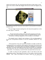
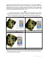
Application of Ortho-SUV Frame: Clinical Cases
Application of Ortho-SUV Frame in fracture treatment
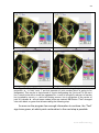
Application of Ortho-SUV Frame in diaphyseal deformities
Application of Ortho-SUV Frame in metaphyseal deformity
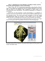
Application of Ortho-SUV Frame in Foot Deformity Correction
Application of Ortho-SUV Frame in Treatment of Knee Joint
Stiffness
page
4
9
9
13
19
20
20
20
24
25
30
30
31
35
35
36
36
40
45
47
48
48
49
53
54
59
63
65
67
69
75
79
81
82
88
90
95
100
109
109
112
121
127
132
www.ortho-suv.org
4
7.
8.
8.1.
8.2.
8.3.
9.
Tips and Tricks for Using the Ortho-SUV Frame
Instead of the conclusion
Legalization
Ortho-SUV Frame training courses and workshops
Where to acquire
References
- Appendix 1
135
141
141
141
141
142
144
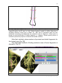
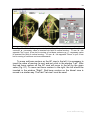
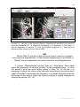
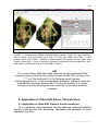
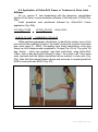
1. Introduction
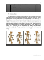
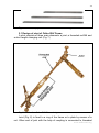
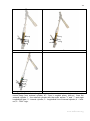
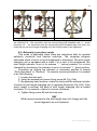
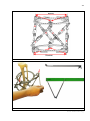
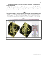
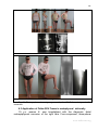
In the correction of complex multi-component and multiplanar deformities
(http://www.ortho-suv.org/images/stories/deform_class2.jpg) using the Ilizarov
frame, unified reduction nodes have to be replaced three to five times (Fig. 1).
Every frame re-assembly involves a change in the reductional units and is a
highly laborious process in which there is additional patient exposure to
radiation. Sometimes, due to the peculiarities of frame assembly (external
supports are not oriented at a right angle to the axes of the bone fragments, a
bone is not at the center of a support, the support for some reason is not
closed, etc.), correction of one component can lead to the secondary
translation of other(s). These secondary translations will, in turn, require
correction and therefore additional frame re-assembly [Solomin L.N. et al.,
2009].
a
b
www.ortho-suv.org
5
c
d
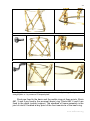
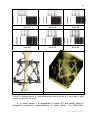
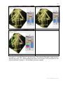
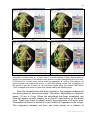
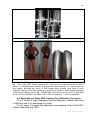
Fig. 1. To correct a multi-component deformity, the Ilizarov frame has to be
reassembled three to five times. a – lengthening. b - correction of an angular deformity and
translation in the frontal plane. c - correction of an angular deformity and translation in the
sagittal plane. d - correction of a rotation
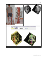
Certainly, the problem of the directed accurate moving of object in
three-dimensional space demands the decision not only in orthopedic
surgery, but also in many branches of technique. One of perspective
directions in the given area is application of hexapods. Hexapods
structurally consist of two (basic and mobile) platforms to be connected by
six telescopic rods of a special design, so-called struts.
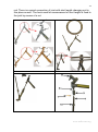
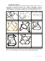
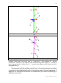
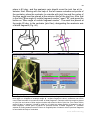
The ways in which the struts connect to each other and to the
platforms differ and depend upon the author’s approach (Fig. 2). The
number of struts is not connected with the number of planes and the
degrees of freedom that the platforms must have relative to each other:
when five struts are used, the system loses its stability, while seven struts
causes overstraining.
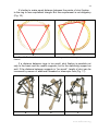
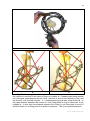
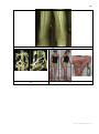
The first hexapod was proposed by Gough in 1947 [Bonev I., 2003] for
testing wheels exposed to combined forces (Fig. 2a). Ceppel, in 1962,
unaware of Gough’s invention, created a similar mechanism while
developing a vibration device (Fig. 2b). Stewart, in 1965 [Bonev I., 2003],
proposed a platform on the basis of the original hexapod (Fig. 2c).
www.ortho-suv.org
6
a
b
www.ortho-suv.org
7
c
Fig. 2. Hexapods. a - Gough's system. b - Ceppel's system. c - Stewart's platform
[Bonev I., 2003]
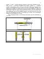
Initial length of each of struts corresponds to initial position of a mobile
platform; final length of each of strut agrees with needed position of mobile
platform. Change of length even of one strut leads to displacement mobile
platform relative to basic one in three planes. Therefore for necessary
displacement of a mobile platform relative basic needs computer
navigation. The task of the software is to calculate required change of
length of each strut using some data input.
There are active and passive navigation in robotics. With reference to
considered devices at active navigation the computer, having received
necessary coordinates of due position of an object (in this case - a mobile
platform) takes all necessary parameters for achievement of result "itself".
If the operator approves modeled result, the device for active computer
navigation steers a mechanism to carry out the directed movement. The
autopilot works in the same way.
At passive navigation the operator put in a computer necessary
coordinates of position of a mobile platform and parameters to describe its
initial position, including initial strut lengths, as well. After that the software
calculates necessary change of lengths for each of strut. Then the operator
changes length of each of strut, to achieve due position of mobile platform.
A car navigator may serve as an example.
In orthopedics, the hexapod may be considered as an universal
reduction unit to allow the movement of one platform (one basic support,
with the bone fragment fixed inside) relative to another by the shortest
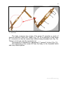
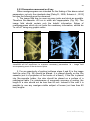
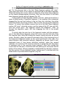
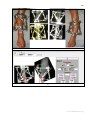
“integral” trajectory. The first “orthopedic hexapod” was patented in 1985 in
France by Philippe Moniot [Paley D., 2011]. At the beginning of 90th years
of the last century in the Ilizarov Russian Research Center the device
shown in Fig. 3a was developed [Shevtsov V.I., 2008, unpublished data].
www.ortho-suv.org
8
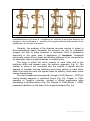
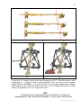
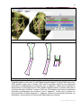
However, these frames were not clinically used, partly due to the lack of
software.
a
b
c
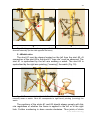
Fig. 3. Orthopedic hexapods. a – device created in Ilizarov Russian Research
Center. b – Taylor Spatial Frame. c - Ilizarov Hexapod System
First orthopedic hexapods, used clinically and sold commercially,
appeared in USA and Germany. Those are Taylor Spatial Frame – TSF (Fig.
3b), with its usage started in 1994 and Ilizarov Hexapod System device – IHS
(Fig. 3c), developed in 1995 [Seide K. et al., 1999]. These devices are
becoming more and more popular at fracture treatment and long bone
deformity correction due to the possibility to implement mathematical
precision of the procedure without resorting to repetitive changes of unified
reduction units [Paley D., 2005; Rozbruch, S.R. et al., 2006; Marangoz S. et
al., 2008; Seide K. et al., 2008; Solomin L.N. et al., 2008; Dammerer D. et al.,
2011]. Original transosseous hexapod (Ortho-SUV Frame) was developed in
Russia in 2006.
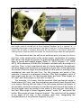
There is an incorrect opinion, that all known orthopaedic hexapods
work using Stewart platform [Taylor J.C., 1997; Seide K. et al., 1999; Paley
D., 2005]. However, IHS and TSF are closer to Gough’s and Ceppel’s
platforms (Fig. 2a,b). Ortho-SUV Frame reminds Stewart platform from outside.
This device was made on the basis of Solomin-Utekhin-Vilensky platform
(SUV-Platform), featuring unique construction and kinematics. Only 3 struts
connect to each ring. The other 3 struts connect to the side of another strut.
The information about the distance between the sides of the triangle
formed at each ring by the strut connection is fed into the computer.
Because only 3 struts connect to each ring, thus forming a triangle between
the connection points, the computer identifies a plane for each triangle
using only the strut lengths and the length of the sides of the 2 triangles.
The beauty of this frame is that for the first time it is independent of the size
www.ortho-suv.org
9
and shape of the rings and the math is much easier. This is by far the
most modular of all the 6 axis correction frames [Paley D., 2011].
Due to improvements, Ortho-SUV Frame succeeds its analogs by a
number of design features, its reductive potential and rigidity of the
osteosynthesis. Additionally, Ortho-SUV Frame is equipped with advanced
software.
Indications for application of Ortho-SUV Frame
1. Fractures (except intra-articular):
- Closed fractures;
- Open fractures;
- Open fractures in conjunction with soft tissue damage such as
burns, soft tissue extensional defects;
2. Consequences of the fractures:
- non-unions;
- malunions;
- posttraumatic deformities;
- osteomyelitis, including bone defects;
3. Long bone deformities:
3.1. congenital deficiency (fibular hemimelia, congenital femoral
deficiency, tibial aplasia etc.);
3.2. Aquired deformities:
-post traumatic;
-post infectious;
- idiopathic;
- bone diseases leading to deformity (Hypo-, Pseudo-,
Achondroplasia; Rickets; Blount; enchondromatosis;
mucopolysaccharidosis etc.);
4. Congenital limb length discrepancies;
5. Foot deformities (including clubfoot; Charcot-Marie Disease etc.);
6. Joint stiffness of elbow, knee and ankle joints of any etiology;
7. Old subluxations in elbow, knee and ankle joints;
8. Aesthetic deformities;
9. Reconstructive procedures (for example: pelvic support osteotomy);
10. Arthrodiastasis.
Further information featuring construction and advantages of hardware
and software will be considered below.
2. Design of Ortho-SUV Frame
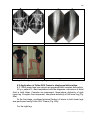
Two external supports comprise the Ortho-SUV Frame (Fig. 4), one
basic and the other mobile. These are united by six struts connected in
www.ortho-suv.org
10
series. Together, these parts constitute the “universal reduction unit”
mentioned above. The basic ring, with the aid of the transosseous
elements, fixes the main bony fragment, while the mobile support holds the
bony fragment to be transported. If necessary, the rigidity of the
osteosynthesis can be increased by using additional stabilizing supports.
a
b
Fig. 4. Ortho-SUV Frame design. а – standard assembly. b – assembly completed
with stabilizing support. 1 – basic (proximal, reference) support; 2 – mobile (distal,
corresponding) support; 3 – struts; 4 – stabilizing support
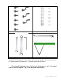
Ortho-SUV Frame’s standard set (Fig. 5) includes:
- six standard(medium) size struts;
- six ring connection plates straight;
- three ring connection plates Z type;
- labels of strut numbers (set of 6);
- X-ray markers of struts (set of 6);
- two spanners 12 mm;
- two spanners 8 mm;
- triangular measurement device;
- Allen key;
- hasp-key (Fig. 25).
www.ortho-suv.org
11
a
b
www.ortho-suv.org
12
c
d
e
f
Fig. 5. A standard Ortho-SUV Frame’s set. a – the full set. b – struts. c - plates
(straight and Z-shaped). d – strut number clips and X-ray positive strut number markers.
e – wrenches and a screwdriver. f – triangular measurement device
Strut length changing units of short and long sizes, a set of threaded
rods of various lengths (Fig. 6) can be taken additionally.
www.ortho-suv.org
13
Fig. 6. Additional equipment: threaded rods of different lengths
2.1 Design of strut of Ortho-SUV Frame
A strut consists of three main elements: a joint, a threaded rod M6 and
a strut length changing unit (Fig. 7)
Fig. 7. Strut’s of an Ortho-SUV Frame design
Joint (Fig. 8) is fixed to a ring of the frame or to plate by means of a
nut. Other end of joint with the help of coupling is connected to threaded
www.ortho-suv.org
14
rod. There is a swivel connection of joint with strut length changing unit in
this place as well. The hook used for measurement of strut length is fixed to
the joint by means of a nut.
a
b
www.ortho-suv.org
15
c
d
e
Fig. 8. Design of a joint of Ortho-SUV Frame’s strut. a – the joint with swivel
connection to strut length changing unit of the next strut. b – fixing a strut to the ring. c –
fixing strut to the plate. d - disassembled clutch. e - assembled clutch. 1 – joint; 2 –
threaded tail; 3 – fixing nut; 4 – threaded rod; 5 – strut length changing unit; 6 – strut
length changing unit of the next strut; 7 – hook; 8 – threaded tail with L-shaped groove;
9 – coupling; 10 – small lock-nut; 11 – straight plate
Strut length changing unit (Fig. 9) consists of a body, a connecting nut,
a threaded clutch and lock-nuts. The body and threaded clutch have 12
mm rust flies.
www.ortho-suv.org
16
Fig. 9. Strut length changing unit. 1 – body; 2 - connector nut; 3 - threaded clutch;
4 - lock-nuts
The body encloses two screws. The screw #1 provides a mode of
fracture reduction (“fast strut” mode) (Fig. 10). At a relaxation of the screw
#1, connector nut can be moved (by rotation) along threaded rod (Fig. 10).
There is a lock-nut over the connector nut.
The screw #2 is intended for “adjustment” ("reverse") of strut (Fig. 10).
The tightening of the screw #2 fixes the body to the threaded clutch
and they rotate together.
www.ortho-suv.org
17
a
b
Fig. 10. Body of strut length changing unit. a - the screw #1 is loose; connector nut
is moved away from the body. b - connector nut is moved into the body, screw #1 and
lock-nut are fixed. 1 - screw #1; 2 - screw #2; 3 - connector nut, 4 - lock-nut
The clutch of strut length changing unit (Fig. 11) consists of two right
threaded cylinders (external and internal). The external cylinder has a scale
with a division value of 2 mm. In addition there are arrows "+" and "-", and
eight longitudinal lines. The internal cylinder has a strut length change
indicator. It moves inside the scale of the external cylinder. There is a
longitudinal line on the internal cylinder as well. External end of internal
cylinder is pivotally connected to the joint of previous strut. The logo "SUV"
is applied here (Fig. 11).
www.ortho-suv.org
18
a
b
с
Fig. 11. Clutch of strut length changing unit. a – view in coronal plane, lock-nut is
moved away from external cylinder. b – view in sagittal plane, lock-nut fixes the
external cylinder. 1 - the external cylinder with the scale, arrows "+" and "-", and eight
longitudinal lines; 2 - internal cylinder; 3 - longitudinal line of internal cylinder; 4 – locknut; 5 - "SUV" logo;
www.ortho-suv.org
19
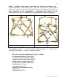
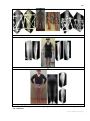
2.2 External supports
Supports from any circular external fixation devise may be used to
assemble an Ortho-SUV Frame (Fig. 12a,d,g). Additionally, supports
comprising 1/2, 2/3, and 5/8 of a ring (Fig. 12b,e) are possible to use, as
well as supports of any shape: triangular, oval, or rectangular (Fig.12 c,f,h).
a
b
c
d
e
f
g
h
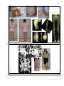
Fig. 12. In the assembly of an Ortho-SUV Frame, supports of various shapes and
types can be used. a,d,g – supports from a range of circular external fixation devices.
b,e –1/2, 2/3, 5/8 rings. c,f,h – oval, triangular, and polygonal shaped supports
www.ortho-suv.org
20
3. Ortho-SUV Frame Assembly
The number of supports in frame modules as well as the number and
type of transosseous elements to insert in each case are chosen on the
basis of knowledge in the biomechanics of external fixation and following
principles of a method of external fixation frame assembly (Solomin L.N.,
2008, 2013).
NB!
Each bone fragment must be strongly fixed to rings. Rigidity of fixing of
each bone fragment to a ring should exclude errors of correction of
deformation due to displacement of the bone fragment inside the ring. For
example, it happens because of insufficient number of wires and half-pins
and (or) their incorrect spatial orientation.
3.1 Supports Assembly
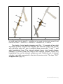
Any angle of support assembling is possible. Bone fragments can be
located both in the external support centre, and off the ring centre (Fig. 13).
a
b
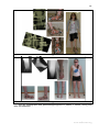
Fig. 13. At Ortho-SUV Frame assembling rings can be placed both perpendicular
to an axis of bone segment and at any random angle, bone fragments can be located in
the centre of rings and off the ring centre as well. a – AP view. b – Lateral view
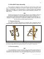
3.2 Strut assembling
NB!
For simplification of strut connection, they should be preassembled as
it is shown in Figs. 5b and 14a. A “preassembled strut” consists of a joint, a
threaded rod and attached to the joint strut length changing unit of the next
strut.
www.ortho-suv.org
21
All the six preassembled struts are interconnected as it is shown in
Fig. 14b. Special dismountable strut number labels (clips) are used for
designation of number of each of struts (Figs. 5d and 14a).
a
b
Fig. 14. Set of struts for Ortho-SUV Frame. а – full set, with arrows pointing the
clips indicating strut number. b – interconnected struts
Struts can be fixed to the ring directly, and by means of straight or Zshaped plates as well (Fig. 15).
www.ortho-suv.org
22
a
b
c
Fig. 15. Variants of strut fixation to support. a - directly to ring. b - by means of
straight plate. c - by means of Z-shaped plate
Struts are fixed to the basic and the mobile rings at three points. Struts
##1, 3 and 5 are fixed to the proximal (basic) ring. Struts ##2, 4 and 6 are
fixed to the distal (mobile) support. The standard of frame assembly is the
joint of strut #1 located at any point of the front semicircle of the basic ring.
www.ortho-suv.org
23
It’s better to make equal distance between the points of strut fixation
to the ring to form equilateral triangle. But this requirement is not obligatory
(Fig. 16).
a
b
Fig. 16. Fixation of struts to support. a – making equilateral triangle. b – random
fixation
If a distance between rings is too small, strut fixation is possible not
only to the basic and the mobile supports, but to the stabilizing support as
well. If the distance between supports is “too much”, length of strut can be
increased by means of additional threaded or telescopic rods (Fig. 17).
a
b
c
www.ortho-suv.org
24
d
Fig. 17. Abilities of Ortho-SUV Frame assembling. a - "standard" configuration:
struts are fixed directly to the basic and mobile supports. b - distance between supports
is not enough for strut fixation directly or using straight plates. Therefore Z-shaped
plates are used. c - distance between support is not enough for strut fixation by means
of Z-shaped plates. Therefore some struts are fixed to stabilizing support. d - increasing
strut length with the help of telescopic rod
NB!
At any mentioned variant of frame assembly two rules must be
observed: “Logo rule” and “Watch rule”.
1. “Logo rule”
A logotype “SUV” marked on the struts must be always directed
externally (to the side opposite the bone) (Fig. 18).
www.ortho-suv.org
25
a
b
Fig. 18. “Logo rule”. a,b - logotype “SUV” marked on struts must be always
directed externally (to the side opposite the bone)
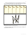
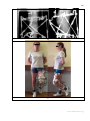
2. «Watch rule»
The strut #1 must be always located on the left from the strut #2. At
connection of the strut #2 to the strut #1 “logo rule” must be observed. The
strut #1 is symbolized by the left arm wearing a watch. The strut #2 is
symbolized by the right arm pointing (“covering”) the watch (Fig. 19).
Fig. 19. The mnemonic “watch rule”. Strut #1 corresponds to left arm, i.e., arm that
normally wears a watch. Strut #2 corresponds to right hand, pointing (covering) the
watch
The positions of the struts #1 and #2 should always comply with this
rule regardless of whether the frame is applied to the left or to the right
limb. Further numbering is done counter-clockwise. Thus joints of struts
www.ortho-suv.org
26
##1, 3 and 5 are fixed to the basic (proximal) support; joints of the struts
##2, 4 and 6 – to the mobile (distal) support (Fig. 20).
a
b
Fig. 20. Struts numeration. a,b - no matter which anatomic side is involved, the
positioning of struts #1 and #2 must comply with the “watch rule” and made counter
clock-wise. struts ##1, 3 and 5 are fixed to the basic (proximal) support; joints of the
struts ##2, 4 and 6 – to the mobile (distal) support
www.ortho-suv.org
27
The algorithm of Ortho-SUV Frame assembling is illustrated in Fig. 21.
Note, that before strut connection, the screw #1 (Fig. 10а) must be loosed
in order that connector nut (Fig. 10b) should have a possibility to be freely
moved into the strut length changing unit.
a
b
assembling proximal (basic) ring
assembling distal (mobile) ring
c
d
fixing strut #1 to basic ring
insertion of threaded rods of strut #2 into
strut length changing unit of strut #2 (it is
fixed to the joint of strut #1). Fixing strut
(joint) #2 to distal (mobile) ring
www.ortho-suv.org
28
e
f
insertion of threaded rods of strut #3 into
strut length changing unit of strut #3 (it is
fixed to the joint of strut #2). Fixing strut
(joint) #3 to proximal (basic) ring
insertion of threaded rods of strut #4 into
strut length changing unit of strut #4 (it is
fixed to the joint of strut #3). Fixing strut
(joint) #4 to distal (mobile) ring
g
h
insertion of threaded rods of strut #5 into
strut length changing unit of strut #5 (it is
fixed to the joint of strut #4). Fixing strut
(joint) #5 to proximal (basic) ring
insertion of threaded rods of strut #1 into
strut length changing unit of strut #1 (it is
fixed to the joint of strut #6). Fixing strut
(joint) #6 to distal (mobile) ring. Note, that
all connector nuts are at some distance
from strut length changing unit (pointed by
arrows)
www.ortho-suv.org
29
i
j
insertion of connector nuts into the body at osteotomy struts ##1, 3 and 5 should be
of strut length changing unit. Fixing screws
temporarily disconnected from proximal
#1. Stabilization of strut length changing
support
units by lock-nuts
Fig. 21. Step-by-step Ortho-SUV Frame assembling
Hereby in Ortho-SUV Frame assembling:
- external supports of any shape and type, excluding monolateral and
arch supports, can be used;
- supports can be placed at any random angle to bone fragments axis;
- the bone can be placed in the centre of support as well as
eccentrically;
- struts can be fixed to supports directly as well as using straight or Zshaped plates;
- the struts can be fixed not only to basic and mobile supports but also
to stabilizing supports;
- the places of struts fixation to supports can be chosen by a surgeon
randomly. It’s better to make equal distance between the points of fixation
to form equilateral triangles. But this term is not obligatory;
- the strut length is formally not limited and depends on the length of
threaded rods used.
None of these parameters requires additional and special data to be
input in the software.
www.ortho-suv.org
30
4. Modes of Ortho-SUV Frame operation
For practical reasons, the distal (mobile) support is moved relative to
the proximal (static, basic) support. A length change of even one of the
struts will cause the mobile support to dislocate in three planes. By
changing the lengths of every strut, displacement of the mobile support
over the required direction and distance is achieved. The amount of the
length change for every strut is calculated by a computer program.
There are two modes of operation for an Ortho-SUV Frame:
1. «Fast struts» mode;
2. «Deformity correction» mode.
4.1 «Fast Struts» mode
This mode is used for acute fracture reduction or when deformity
correction is implemented under visual control or fluoroscopy. The
procedure starts with the loosening of the large lock-nuts, moving them, by
their rotation, away from the strut length changing unit. Fixing screws #1
are loosened using the hexahedral screwdriver (Fig. 22а). The connector
nuts are moved behind the lock-nuts (Fig. 22b). The next step is a
reduction, implemented by manually moving the rings relative to one
another (Fig. 22c). The connector nuts are then moved along the threaded
rods until each one locks with its respective strut length changing unit.
Fixing screws #1 are tightened (Fig. 22d). Finally each strut length
changing units must be fixed by lock-nuts.
a
b
www.ortho-suv.org
31
c
d
Fig. 22. Fracture reduction in fast strut mode. а – fixing screws #1 of all the struts
are loosened. b – the connector nuts are moved along the threaded rods. c – acute
reduction. d – the connector nuts are moved along the threaded rods until each one
locks with its own strut length changing unit; the fixing screws #1 are tightened
4.2 «Deformity correction» mode
This mode is applicable when there are indications both for gradual
deformity correction and fracture reduction. The computer program
calculates which of struts is to be lengthened or shortened. The strut length
changing unit is equipped with a scale. For a strut to be lengthened, the
strut length indicator is set in its extreme “−” (minus) position. For a strut
intended for shortening, the indicator is set in its extreme “+” (plus) position.
Procedure on moving the indicator in necessary position is named
“Strut adjustment” or "Reverse". To execute reverse procedure it is needed
to do the following:
1. Loosen the lock-nuts.
2. Using the screwdriver loosen fixing screw #2 (Fig. 23а).
3. By opposing hand motions, rotate the body and the external cylinder
of clutch of strut length changing unit in opposite directions (Fig. 23b). If the
strut’s length is minimal, the body of strut length changing unit is rotated
clockwise; if it is maximal, rotation is counter-clockwise.
4. Tighten fixing screw #2 and the lock-nuts.
NB!
While reverse procedure the strut length does not change and the
bone fragments are not displaced.
www.ortho-suv.org
32
a
d
b
c
e
Fig. 23. Adjustment of a strut (reverse procedure). а – scale before the procedure:
the indicator is set in its extreme «+» position. b – loosening fixing screw #2. c – the
body and the external cylinder of clutch of strut length changing unit are counterrotating. d – fixing screw #2 is tightened. e – the scale after the procedure: indicator is in
its extreme «-» position. The strut length has not been changed!
As it was already specified, the tightening of the screw #2 fixes the
body to the clutch of strut length changing unit owing to what they rotate
together.
To change strut length lock-nuts are loosened and the body with fix to
it clutch are rotated (Fig. 24). As it was already mentioned, there are
www.ortho-suv.org
33
arrows "+" and "-" on the external cylinder of the clutch. Rotation of the
body in the "+" direction increases strut length; rotation in "-" direction
results in shortening of strut. Full turn of the body (360 deg.) changes strut
length up to 2 mm. The scale interval is 2 mm. Accordingly, 45 deg. turn
changes strut length to 0.25 mm. To control gradual, 0.25 mm, change of
strut length, there are eight longitudinal lines on the external cylinder and
one longitudinal line on the internal cylinder. Turn from one line up to the
next line corresponds the turn of the body by 45 deg., and, accordingly,
change of strut length by 0.25 mm.
After changing length of strut body and clutch must be stabilized by
lock-nuts.
a
b
www.ortho-suv.org
34
c
d
e
Fig. 24. “Deformity correction” mode: gradual changing length of strut. a – loosing
of lock-nuts. b - rotation of the strut length changing unit in "+" direction leads to strut
lengthening; in "-" direction leads to strut shortening. Turn “from line to line” changes
length of strut by 0.25 mm. с - full turn (360 deg.) of strut length changing unit changes
strut length by 2 mm. The scale interval is 2 mm. d – strut is rotated by hand or, at strut
tension, by spanner 12 mm. e – fixing of lock-nuts.
NB!
Sometimes the scale length is not sufficient for a fragment
displacement to be corrected completely. In such cases the reverse
www.ortho-suv.org
35
procedure (Fig. 23) must be repeated. Thus, the maximal strut length is
limited only by length of threaded rod used.
NB!
There are no situations when both fixing screws (#1 and #2) are
loosened at the same time. The loosing of the screw #1 allows “fast strut”
mode to be completed. The loosing of the screw #2 is necessary for
“reverse procedure”. At gradual deformity correction both screws must be
tightened.
The precisely controlled relocation of bone fragments requires that the
amount of length change be calculated for every strut. This can be done
using specialized software.
5. Software for the Ortho-SUV Frame
5.1 General information
The program for working with the Ortho-SUV Frame was written using
the language “C++ Builder.” Its volume is about 1.400 kb. To install the
program, copy the executable file onto a hard disc. The minimal
requirements are: IBM PC-compatibility, operating system Windows 2000,
XP or Vista, processor with a minimal quality of the DX486 and a minimum
frequency of 1.5 GHz, and a memory of 256 Mb RAM. Installation requires
at least 10 Mb of disk space. Color display with a minimal resolution of 800
x 600 pixels is necessary.
Software is available as a folder “SUV-Software vр. ******”. There is a
number of the version of the program instead of "*******", for example,
“SUV-Software vр. 1.0”. The folder has two files: “SUV-Software vр.exe”
and "winspool.dll". The later version has greater number, than the previous
one. Updated software is placed on website http://ortho-suv.org.
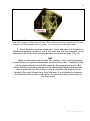
Program works with digital roentgenograms saved in formats .bmp and
.jpg. The software is protected from non-authorized use by HASP-key (Fig.
25). The HASP-key as an USB-charm is included into the complete set of
Ortho-SUV Frame. The appropriate HASP-driver should be installed on a
computer. The driver can be taken from the website http://www.aladdinrd.ru/support/downloads/haspsrm/. It is necessary to download and install
the driver “Sentinel HASP for Windows. Version 6.22 (the interface: GUI)”.
Before start your first work with the program, please, follow few
essential steps described in Appendix 1.
www.ortho-suv.org
36
Fig. 25. Before software use the HASP-key must be inserted into USB-port of a
computer. The red indicator confirms, that the program is ready to work
Working with the program involves advancing through its sequence of
13 steps. At every step, if necessary, the operator can return to the
previous one. If the obligatory actions required at every given step are not
performed, moving to the next step is not possible.
5.2 The parameters must be input into the software
Two groups of parameters must be input into the computer program:
Group 1. Parameters, measured on the frame (12 parameters) and at
making roentgenograms (2 parameters);
Group 2. The parameters determined on roentgenograms (14
parameters).
The first group of parameters can be taken using measuring tools.
Parameters of the second group are found using tools of the software.
5.2.1 Parameters, measured on the frame
The 12 parameters measured on the frame are strut length (6
parameters) and the side lengths of the triangles (6 parameters) whose
apexes are the centers of the nuts fixing the strut joints to the ring or plate.
Strut length is a distance between the hook located on joint and the
end of the strut length changing unit (Fig. 26). It is a mistake to measure
the distance from the hook up to the end of the threaded rod!
www.ortho-suv.org
37
a
b
c
Fig. 26. Strut lengths measurement. а – strut length “L” is measured between strut
hook and ending point of strut length changing unit. It is a mistake to measure distance
from hook up to end of threaded rod! b – measurement using a ruler or measuring tape.
c – measurement by laser range-finder
The sides of the triangles are measured between the centers of the
nuts that fix the joints to the rings or to the plates (Fig. 27). It is erroneous
to measure the distances between the centers of the nuts that fix the plates
to the rings!
For the basic ring, the sides of the triangle are indicated as A1 (Base),
B1 (Base), C1 (Base). Thus, A1 (Base) is the distance between joints #1
and #3; B1 (Base) is between joints #3 and #5; and C1 (Base) is between
joints #5 and #1.
For the mobile ring, the sides of the triangle are indicated as A2
(Mobile), B2 (Mobile), C2 (Mobile). Thus, A2 (Mobile) is the distance
between joints #2 and #4; B2 (Mobile) is between joints #4 and #6; and C2
(Mobile) is between joints #6 and #2. All measurements are made using the
special measuring tool (Fig. 27).
www.ortho-suv.org
38
a
b
www.ortho-suv.org
39
c
d
e
Fig. 27. Measuring sides of triangles. а – sides of triangles are measured between
the centers of nuts that fix the joints to rings or to plates. b – measurement using special
tool (triangular measurement device). Note, that one of strut is fixed directly to ring, and
the second - with the help of plate. c – measurement using a laser range-finder. d – in
this case distance between the centres of nuts fixing plates to ring is measured. It is a
mistake! e - in this case the distance between the centre of nut fixing plate of strut #1
and the centre of nut fixing joint #3 to plate is measured. This is wrong measurement!
www.ortho-suv.org
40
5.2.2 Parameters measured on X-ray
When roentgenograms are intended for the finding of the above-noted
parameters, not only the standard rules [Paley D., 2005; Solomin L., 2013]
but also the following must be observed:
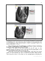
1. The image field has to cover as many joints and struts as possible.
Therefore film-cassette <30 cm in width are inappropriate (Fig. 28). The
image field should contain only the helpful information. Edges of
roentgenograms which do not have the necessary information, should be
"to cut off" using any graphic editor.
a
b
Fig. 28. Image field. a – when a narrow film is used, the number of struts and joints
visualized will be insufficient to measure necessary parameters. b – image field
encompassing most of the struts and joints
2. For an opportunity of scaling (software steps 4 and 5) in the image
field the ruler (Fig. 29) should be placed. It is placed directly on the film
cassette (not in a projection of the centre of a bone!). If the film is placed
into film-cassette holder, the ruler should be placed on a surface of a
radiological table. For maintenance of necessary accuracy of scaling, the
length of a ruler should not be less than 80 mm. Instead of the ruler it is
possible to use any roentgen-visible subject of known (not less than 80
mm) lengths.
www.ortho-suv.org
41
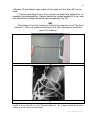
Fig. 29. For an opportunity of scaling the image field must contain roentgen-visible
ruler with length not less than 80 mm. Ruler should be placed directly on the filmcassette or (if film-cassette holder is used) - on a surface of a radiological table
3. Focal distance must be measured. Focal distance is a distance in
millimeters between anode of the X-ray tube and the film cassette. X-ray
equipment often has focal distance sensors or measuring tape (Fig. 30).
NB!
When a radiopaque ruler is used (for scaling – step 4 in the program),
a focal distance is measured between anode and the ruler. Therefore, if the
ruler is placed directly on the film-cassette, the general rule works. But
when the film-cassette is placed into the radiological table holder and the
ruler is positioned on the surface of the X-ray table, the distance from
anode to the ruler is taken as a focal distance. It is a mistake to measure
the distance from anode to the center of a bone and placing the ruler on
the bone level.
www.ortho-suv.org
42
Fig. 30 Measuring focal distance (two parameters: for AP and Lateral views)
4. X-ray beam center must be indicated on the roentgenogram. For
this purpose, a small (about of a cent coin in size), usually cross-shaped
marker is placed on film-cassette, where is the center of X-ray beam (Fig.
31). While X-ray examining, make sure that this beam center marker did
not overlap with any radiopaque parts of the frame, such as struts or rings.
a
b
Fig. 31. Beam center identification. a – self-adhesive X-ray-positive mark to
visualize the beam center. b – this mark points the beam center on the film
5. To facilitate the strut number identification, special radiopaque
markers with bar-codes are used (Fig. 32).
www.ortho-suv.org
43
a
strut #1
b
strut #2
c
strut #3
d
strut #4
e
strut #5
f
strut #6
g
h
Fig. 32. Strut markers. a-f – markers of struts ##1-6, schemes and image of "barcodes" on roentgenogram. g – strut markers are fixed on struts. h - x-ray image of strut
markers (pointed by arrows)
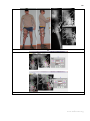
6. In some cases it is impossible to make AP and lateral views in
tangential projections (perpendicular to each other). For Ortho-SUV
www.ortho-suv.org
44
software AP and lateral views made at the angle not less than 45º can be
used.
7. If there are analog X-rays, they must be converted into digital form, for
example, by photographing. Camera should be located parallel to X-ray view
box and the X-ray image should be taken completely (Fig. 33).
NB!
The distance from the camera up to the X-ray view box is not "the focal
distance". The focal distance which was at X-ray examination should be
input into software.
a
b
Fig. 33. Converting analog X-rays into digital format. а – camera should be located
parallel to X-ray view box. It is not "the focal distance"! b – image includes struts, joints,
scaling ruler and marker of beam center
www.ortho-suv.org
45
5.3 Working With the Program
After an initial training, including 10-12 calculations, the program
assumes the following standard of work:
- 8-12 minutes in case of fractures and shaft deformities;
- 12-15 minutes in case of epimetaphyseal deformities and
reconstruction surgeries.
It is necessary to provide maximum accuracy of each parameters input
(Steps 1,6,7,10 and 11) and proper performance of the procedures
required (Steps 4-10 and 12). It will provide "ideal" reduction and deformity
correction.
NB!
The folder “Ortho-SUV Frame” must be created on the working table of
the computer. This folder should contain folders "SUV-Software" (for files of
the software) and "Cases" (for clinical cases).
Before working with the program it is necessary to create a folder with
the title of the clinical case, for example “Case 1”. AP and lateral view of
the patient must be placed in this folder (Fig. 34).
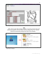
Fig. 34. The clinical case folder should contain patient’s AP and lateral view
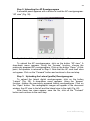
To start working, double-click “SUV.exe” file. Program window
appears. Press the "New document" button. New document will be created
with its first page entitled «Step 1» (Fig. 35).
www.ortho-suv.org
46
Fig. 35. Program window step 1 after new document has been created
NB!
After “clinical case” file had been created, it must be saved in the same
folder where patient’s AP and lateral view are placed (Fig. 36). This file
should be saved after passing each step of the software.
Fig. 36. Clinical case folder must contain patient’s AP and Lat view as well as SUV-file
created by the software
www.ortho-suv.org
47
NB!
If for some reason difficulties have occurred (usually associated with
incorrect usage), sent the folder contained X-rays and SUV-file to the
following email address: [email protected]. In the accompanying
message, explain in detail the problem that has been encountered. To
resume working, it is usually enough to re-start the program and, obviously,
avoid one’s previous mistakes.
Step 1: Input of Strut Lengths and Those of the Sides of the
Triangles
Fill in the window “Patient data” by typing in the patient’s surname,
name, age, and diagnosis as well as the modeling date (Fig. 37).
Fill in the fields “Strut 1–Strut 6” (Fig. 37) by inserting the lengths of the
corresponding struts, as measured according to the rules described in
Sect. 5.1 (Fig. 26).
Fill in the fields “Triangles A1 (Base), B1 (Base), C1 (Base), A2
(Mobile), B2 (Mobile), C2 (Mobile)” by typing in the respective sizes of the
sides of the triangles whose apexes are the centers of the nuts fixing the
strut joints to supports or to plates. The rules for measuring the sides of the
triangles are provided in Sect. 5.1 (Fig. 27). There are scheme-prompt at
this step window.
After completion of these fields and saving the file, click on the
“Forward” button and continue to the next step.
Fig. 37. Data input in Step 1. 1 – patient data; 2 – strut lengths; 3 – triangle side lengths;
4 - scheme-prompt
www.ortho-suv.org
48
Step 2: Uploading the AP Roentgenogram
A movable panel appears with a button to load the AP roentgenogram:
“AP view” (Fig. 38).
Fig. 38. Ortho-SUV program window in Step 2: Uploading the AP view
To upload the AP roentgenogram, click on the button “AP view.” A
drop-down menu appears. Using the “browse” function, choose the
previously prepared AP roentgenogram. Click on the button “Open.” At this
point, the operator is returned to Step 2. Note that the AP view itself does
not appear. Click on the “Forward” button and continue to the next step.
Step 3: Uploading the Lateral (profile) Roentgenogram
To upload the lateral digital roentgenogram, click on the button
“Lateral” (Fig. 39). A drop-down menu appears. Using the “browse”
function, choose the previously prepared lateral roentgenogram. Click on
the “Open” button. Two radiographic images will appear in the document
window: the AP view to the left and the lateral view to the right (Fig. 40).
After these two views appear, save the file, click on the “Forward”
button and continue to the next step.
www.ortho-suv.org
49
Fig. 39. Ortho-SUV software window after Step 3
Fig. 40. Ortho-SUV software window after Step 3, in which the AP and lateral
views appear
Step 4: Scaling of the AP View
At the step 4 in a window of the program appear earlier uploaded AP
view, the button “+/-” (“zoom in/zoom out”) and the special tool, so-called
"dumbbell" (Fig. 41). Having pressed by the button “+/-”, the user chooses,
www.ortho-suv.org
50
what he wants to make with the roentgenogram: magnification or reduce
the image. Thus near "+" or "-" appears an appropriate dot index. After that
double click of the left button of the mouse in the field of the
roentgenogram, the user enlarges or reduces the image. The picture is
enlarged (reduced) around of the cursor. It lets make the centre for
magnification (demagnification) any point of the roentgenogram. Moving of
the roentgenogram along the screen is carried out as follows: having
pressed on the left button of the mouse in a field of the roentgenogram and
not releasing the mouse button, the user moves the cursor in that direction
where he wants to move the picture.
Fig. 41. Ortho-SUV software window in Step 4. 1 - AP view; 2 - “+/-” (“zoom
in/zoom out”) button; 3 - tool "dumbbell"
For scaling the AP view, extreme points of the "dumbbell" must be
overlapped with roentgen-visible ruler which is on the roentgenogram (Fig.
29). To move the "dumbbell", place the cursor directly on its center (visible
as a small circle) and, while left-clicking the mouse, move the ruler around
the display to roentgen-visible ruler. After that one of the ends of the
"dumbbell" should be overlapped with one of the ends of the ruler. For this
purpose direct the cursor on one of the ends of the "dumbbell" and, while
left-clicking the mouse, drag it on screen before it coincides to the end of
the ruler.
Due to this, the "dumbbell" is increased in length. Similarly overlap other
end of the “dumbbell” with the opposite end of the ruler. After the length
and position of the "dumbbell" have been set, fill in the field “Interval
www.ortho-suv.org
51
between (AP view)” by typing in the length of the known interval in mm
(Fig. 42); then click on the “Forward” button to continue to the next step.
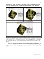
a
b
c
Fig. 42. Ortho-SUV software window in Step 4: «Scaling of AP view». a – prior to
scaling. "Dumbbell" is outside of field of roentgenogram. b – "dumbbell" is moved to
ruler, one of its ends is overlapped with ruler. c – after scaling. Both ends of "dumbbell"
are overlapped with ruler. Field “Interval between” is filled in according length of ruler 80 mm
If for the program the analog roentgenogram was photographed, for
scaling the size of the roentgenogram can be used: its width or length (Fig.
43).
www.ortho-suv.org
52
a
b
Fig. 43. Ortho-SUV software window in Step 4: «Scaling of AP view» (analog
roentgenogram was the initial source). a – prior to scaling. "Dumbbell" is outside of field
of roentgenogram. b – after scaling. Both ends of "dumbbell" are overlapped with ends
of the roentgenogram. Field “Interval between” is filled according to width of the analog
roentgenogram - 298 mm
www.ortho-suv.org
53
Step 5: Scaling of the Lateral View
Lateral view scaling is implemented in the same way as described for
the AP view (Figs. 44 and 45). Click on the “Forward” button to continue to
the next step.
a
b
Fig. 44. Ortho-SUV software window in Step 5: Scaling of lateral view (digital
roentgenogram was the initial source). a – prior to scaling. "Dumbbell" is outside of field
of roentgenogram. b – after scaling. Both ends of "dumbbell" are overlapped with ruler.
Field “Interval between” is filled in according to length of ruler - 80 mm
www.ortho-suv.org
54
a
b
Fig. 45. Ortho-SUV software window in Step 5: Scaling of AP view (analog
roentgenogram was the initial source). a – prior to scaling. "Dumbbell" is outside of field
of roentgenogram. b – after scaling. Both ends of "dumbbell" are overlapped with ends
of the roentgenogram. Field “Interval between” is filled in according to width of the
analog roentgenogram - 298 mm
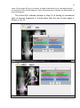
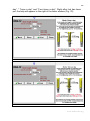
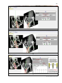
Step 6: Entering the Focal Distance and Beam Center; Indicating
Strut and Joint Projections on the AP View
Type in the value of the focal distance for the AP view, i.e., the
distance between the anode of the X-ray tube and the plate-holder, in the
field “Focal distance (AP view)” in mm (Fig. 30).
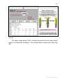
After that on the field of the roentgenogram, mark the X-ray beam
center. For this purpose put "tick" in a field of the panel “Beam center”.
Then bring the cursor to the label on the roentgenogram indicating the
www.ortho-suv.org
55
centre of the beam (Fig. 31) and press the left button of the mouse. In the
field of the cursor a dark blue dagger with the red centre will appear (Fig.
46).
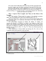
Fig. 46. Ortho-SUV software window in Step 6. The focal distance has been
entered (760 mm) and the X-ray beam center marked. An arrow points to the marker of
the beam center
The next stage involves marking the strut and joint projections on the
AP view (Figs. 47 and 48).
NB!
The strut and joint numbers indicated in the program must be the
same as the strut and joint numbers used in the external fixation device
calculations. Arbitrary designation of the numbers is not allowed.
The simplest way to identify strut numbers on the roentgenograms is
to use the X-ray-positive markers of the strut numbers (section 5.2, Fig.
32).
NB!
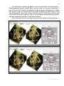
If the projection of any strut or joint is doubtful or invisible (outside the
roentgenogram or is covered by other details of the frame), this strut or joint
can be ignored. The software does not demand a designation of all struts
and joints. As a rule, it is enough to note three struts and two not connected
with them joints. But if AP and lateral view were made not perpendicularly
each other, it is necessary to mark all struts and joints that can be seen.
In order to mark the strut projection, click in the field of the strut
appropriate number. Then bring the cursor to the centre of joint the same
number. Then, while left-clicking the mouse, drag the line along the
www.ortho-suv.org
56
projection of this strut onto the X-ray image (Fig. 47). The line should be
drawn strictly along the strut centre. For correction of position of the line,
bring the cursor to any of its ends, press the left button of the mouse and
move the line in a necessary direction. If the centre of joint is invisible, draw
the line in a projection of a seen part of strut.
NB!
As joints of struts ## 1, 3 and 5 are fixed to the proximal ring, lines for
these struts must be drawn top-down. As joints of struts ## 2, 4 and 6 are
fixed to the distal ring, lines for these struts must be drawn bottom-up.
a
b
c
Fig. 47. Ortho-SUV software window in Step 6: Indicating the strut projection. a - in
field “Strut 1” the tick is put. The cursor is brought to area joint #1 (pointed by arrow). b
– while-pressing left button of the mouse, line in projection of centre of strut #1 is drawn.
с - all well seen struts are marked
www.ortho-suv.org
57
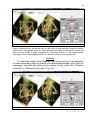
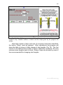
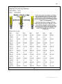
After that projections of strut joints must be drawn. For this purpose
in a field “Projections of joint centers” put a tick opposite to joint number
which is going to be designated. This results in the fact that around of the
point designating the "joint end" of the strut line, a small circle with a small
line appeared. The line of small circle has a red point on its end. Move the
cursor to this point, press the left button of the mouse and move it so that a
line, connecting with small circle became axial line of joint (Fig. 48).
Accuracy of lines drawn in the projection of struts and joints should be
checked up in a mode of image magnification. If some of lines are not
precisely in a projection of an axis of strut or joint, aim the cursor at any of
three red points and while left-clicking the mouse, move the drawn lines in
the necessary direction.
www.ortho-suv.org
58
a
b
c
d
Fig. 48. Ortho-SUV software window in Step 6: Indicating the joint and strut
projection. a – in field “Joint 1” put tick opposite to joint number which is going to be
designated. This results in that around of a point designating the "joint end" of the strut
line, a small circle with a small line appeared. b - cursor is brought to red point of cardan
line (marked by arrow). c - while left-clicking mouse, line in projection of the centre of
joint #1 is drawn. d - all well seen cardan joints are marked. NB! Button "Fwd" changed
color with black on green that allows making the following step
As soon as the program has enough information to continue, the “Fwd”
sign turns green, at which point continuation to the next step is possible.
www.ortho-suv.org
59
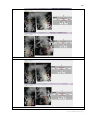
Step 7: Indicating the Focal Distance and Beam Center, and the
Strut and Joint Projections on the Lateral View
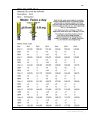
Step 7 (Figs. 49 - 51) is carried out essentially as described for Step 6.
Here, it must again be emphasized that the numbers assigned to the strut
and the joints in the program must correspond to those used in the
corresponding frame calculations. The arbitrary designation of numbers is
not allowed.
As a rule, for the program to work successfully, it is sufficient to
indicate three struts and one joint, with the joint numbered differently from
the indicated struts. The struts and joints indicated on AP and lateral
roentgenograms might not coincide. In other words, the AP view might
feature one set of indicated joints and struts, and the lateral view another.
As soon as the program has enough information to continue, the “Fwd”
button turns green and it is possible to continue to the following step.
Fig. 49. Ortho-SUV software window in Step 7 for lateral view. The focal distance
has been entered (760 mm) and the X-ray beam center marked. An arrow points to the
marker of the beam center
www.ortho-suv.org
60
a
b
c
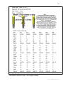
Fig. 50. Ortho-SUV software window in Step 7: Indicating the strut projection on
Lat view. a - in a field “Strut 1” the tick is put. The cursor is brought to area joint #1
(pointed by arrow). b – while-pressing left button of the mouse, line in projection of the
centre of strut #1 is drawn. с - all well seen struts are marked
www.ortho-suv.org
61
a
b
c
d
Fig. 51. Ortho-SUV software window in Step 7: Indicating the joint and strut
projection on lateral view. a – in field “Joint 1” put tick opposite to joint number which is
going to be designated. This results in that around of a point designating the "joint end"
of the strut line, a small circle with a small line appeared. b - cursor is brought to red
point of cardan line (marked by arrow). c - while left-clicking mouse, line in projection of
the centre of joint #1 is drawn. d - all well seen cardan joints are marked. NB! Button
"Fwd" changed color black for green that allows making the following step
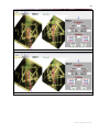
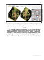
After the forward button has been clicked on, the program analyses all
the data entered at all previous steps. This takes, depending on computer
power, 10 sec to 2 min. When the calculation has been completed, red
lines will appear on both images: six on the AP view and six on the lateral
view. These lines have to exactly match the projections of all strut axes.
Permissible deviation is limited by a strut width as it appears on the image.
The congruency between red lines and struts serves as a criterion of
www.ortho-suv.org
62
correct data input (Fig. 52). If this congruency is present for all the struts,
click “Yes” and continue to the next step.
NNB!!
If even a single red line does not match a strut seen on the
roentgenogram, click “No” to return to Step 7. Then it is necessary to
return to all previous steps and consistently check all data input. Only
when congruency between all red lines and all strut projections is
achieved one may continue to the next step!
a
b
Fig. 52. Ortho-SUV software window in Step 7 after the program has analysed all
data input. a – all red lines match strut projections. Button "Yes" must be pressed. b –
some lines do not coincide with strut projection. It is necessary to press button "No" and
to check up ALL data which were input at each previous steps
www.ortho-suv.org
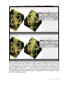
63
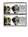
Step 8: Drawing the Bone Contours
The contour of the mobile bone fragment is outlined with a yellow line
on the AP and lateral views. For accurate matching yellow lines to a
contour of a bone fragment it must be made at the maximal magnification.
Note, that length of bone contour has no principle importance for the
software. Therefore it is not necessary to draw contours of all distal
fragment: from the proximal end up to joint line. Length of bone contour 1-2
cm is permitable. But in this case in the Step 11 it will be very difficult to
understand, what final position of distal fragments is recommended by the
software. Therefore recommended length of bone contour must not be less
than 3-4 cm (Fig. 53).
Also it is necessary to take into consideration that axes (mid lines) of
bone contours (Step 9) must be drawn 2-3 cm out of bone contours border.
Therefore the distal border of bone contour must be over 3 cm above the
distal border of the roentgenogram field.
To make a bone contour place the cursor on a cortex of mobile
fragment. Press the left button of the mouse and than release it. Yellow
point will appears on the screen. Move the cursor on other point of the
cortex and press the left button of the mouse again. A line connecting the
new point with the previous one will appear. By successive drawing of
necessary number of lines, make outline of bone fragment (Fig. 53).
If the last fragment of the line is drawn incorrectly, use the button
“Erase the last line.”
Note that in the Step 8 in the panel of tools there is a button of moving
of fields of roentgenograms (Fig. 53). This button is used when it is
necessary to move a field of x-ray picture on the screen, and to increase or
reduce (in a combination with the button zoom in / zoom out) the
roentgenogram. Use the button as follows: pressing left mouse in field of
this button results in appearance of a tick. It means, that the function of
moving is switched on and drawing the bone contour is blocked. Moving xray picture and its reduction / magnification should be done in the same
way as it was described in Step 4. After required action has been done
(moving of a x-ray picture or its reduction / magnification), you must switch
this button off. After that drawing bone contour can be continued.
NB!
Lengths of bone contours on AP and Lat view must be of equal length.
Once the bone contours have been drawn on the AP and lateral views,
click the “Fwd” button.
www.ortho-suv.org
64
a
b
www.ortho-suv.org
65
с
d
e
Fig. 53. Ortho-SUV software window in Step 8. a – arrow points the button of
moving of fields of roentgenograms. On AP view arrow indicates the yellow point made
by cursor. b – yellow line in projection of cortex of distal fragment (AP view) is drawn. c
– yellow bone contours on AP and Lat view are done. Note that bone contours are of
equal length. d, e - possible variants of bone contours of mobile fragment
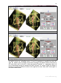
Step 9: Marking the Anatomic Axes of the Bone Contours on the
AP and Lateral Views
To mark the anatomic axis, the cursor is placed in the center of the
bone contours of the mobile bone fragment, 2-3 centimeters above its
proximal end. Pressing the left button of the mouse, make points, which the
program connects in a line. If there are bends of bone fragment, line must
replicate them, because it must be “mid-diaphyseal line of the bone
contour”. Axis of bone contour must be done both on AP and Lat view (Fig.
54).
www.ortho-suv.org
66
If the last fragment of the line is drawn incorrectly, use the button
“Erase the last line.”
After drawing blue lines on AP and Lat view, press button "Fwd". If the
note “Precise the anatomical axes sizes” appears, it is necessary to
remove axes of bone contours and draw the new one which exceeds more
proximal and distal ends of bone contour.
NB!
The anatomic axes of the bone contour must exceed its proximal and distal
ends by 2-3 centimeters. If the X-ray image is short and it is impossible to
draw the blue line above the distal end of the bone contour, the operator
must return to Step 8, remove the bone contour, and draw a new, shorter
one.
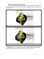
a
www.ortho-suv.org
67
b
Fig. 54. Ortho-SUV program window after completion of Step 9. a - on AP and Lat
view anatomical axes of yellow bone contours are drawn. b – if there are bends of bone
fragment, axes should replicate them, because it must be “mid-diaphyseal line of bone
contour”. The anatomic axes of the bone contour must exceed its proximal and distal
ends by 2-3 centimeters
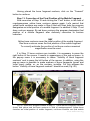
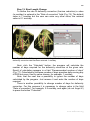
Step 10: Marking the Bone Fragment Axes
Special tools are used to mark the axes of both the basic and the
mobile bone fragments, the bone fragment markers (“trees”). The basic
fragment marker is colored green, and the mobile fragment marker is violet.
So we have a green tree and a violet tree.
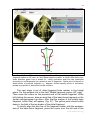
Fragment markers consist of (Fig. 55):
- the axial line (1);
- two centrators (2 and 3);
- the indicator of an angle of axial line positioning (“blue angle”) (4).
Blue angle is placed on one of the centrators;
- the pointer of bone fragment border (“yellow point”) (5). The yellow
point is connected to the red point (6).
www.ortho-suv.org
68
a
b
Fig. 55. Bone fragment markers (a – proximal and b – distal) in Ortho-SUV
software: “green tree” and “violet tree”. 1 – axial line; 2 – first centrator; 3 – second
centrator; 4 – indicator of an angle of axial line positioning (“blue angle”); 5 – pointer of
bone fragment border (“yellow point”); 6 – red point providing moving of yellow point (5)
along axial line (1)
During work with the software axial lines of trees are placed according
to anatomic (mid-diaphysial lines) or mechanical axes of bone fragments. It
depends on what axes (anatomic or mechanical) are used for planning of
deformity correction.
www.ortho-suv.org
69
Setting of fragment markers according to anatomic axes
At first fragment marker of proximal fragment in frontal plane should be
set. For this purpose tick in the field "Base fragment marker (AP view)”.
Then move the cursor of the mouse on proximal end of the basic fragment.
While left-clicking the mouse, draw an axial line of the basic bone fragment
on the frontal roentgenogram top-down. After that the marker of the basic
bone fragment (green tree) will appear (Fig. 56).
If the position of base fragment marker is correct, yellow point will be in
area of distal border of proximal fragment. If an operator has mistakenly
dragged the line not from bottom to top, but from top to bottom, the yellow
point will assume the wrong location, that is at the very top of the fragment
marker. To correct this mistake, remove the tick in the field “Base fragment
marker (AP view)”, place the cursor over the image of the AP view, and leftclick the mouse once. The fragment marker will disappear. Then, go
through the algorithm again, this time dragging the line in the proper
direction.
To strictly align the axis line of the fragment marker with the anatomic
axis of the base bone fragment, place the cursor over the left end of the
first centrator and, while left-clicking the mouse, place this point on the left
cortex. Similarly, place the second outermost point of the centering line of
the base bone fragment marker on the cortex positioned to the right. At a
some distance from proximal centrator (depends on known rules of middiaphysial lines of long bones definition) similarly, place the second
centrator. As a result on AP view the axial line of green tree will take place
of anatomic axis of the proximal bone fragment. After that overlap the
cursor with the red point, connected with the yellow point, and press the left
button of the mouse. Moving upwards or downwards the red point, achieve,
that the pointer of bone fragment border (“yellow point”) coincided with the
distal border of proximal bone fragment (Fig. 56).
a
www.ortho-suv.org
70
b
c
Fig. 56. Ortho-SUV software window in Step 10, at positioning of proximal bone
fragment marker on AP view. a - field “Base fragment marker” is ticked. After that in topdown direction green tree is drawn. b - using centrators axial line has positioned
according to mid-diaphysial line (anatomic axis of fragment). Yellow point is placed on
distal border of proximal fragment. c - diagram. Arrows specify points of centrators,
placed in projection of lateral and medial cortexes
The next stage is set of distal fragment bone marker in the frontal
plane. For this purpose tick in the field "Mobile fragment marker (AP view)".
Then move the cursor on the proximal end of the mobile fragment. While
left-clicking the mouse, draw an axial line of the basic bone fragment on the
frontal roentgenogram top-down. After that the marker of the mobile bone
fragment (violet tree) will appear (Fig. 57). The yellow point should settle
down in the field of the top border of the distal fragment.
To strictly align the axis line of the fragment marker with the anatomic
axis of the base bone fragment, place the cursor over the left end of the
www.ortho-suv.org
71
first centrator and, while left-clicking the mouse, place this point on the
cortical layer positioned to the left. Similarly, place the second outermost
point of the centering line of the base bone fragment marker on the cortex
positioned to the right. At a some distance from proximal centrator
(depends on known rules of mid-diaphysial lines of long bones definition)
similarly, place the second centrator. As a result, the anatomic axis of the
distal bone fragment will be positioned on AP view. After that overlap the
cursor with the red point, connected with the yellow point, and press the left
button of the mouse. Moving upwards or downwards the red point, achieve,
that the pointer of bone fragment border (“yellow point”) coincided with the
proximal border of the distal bone fragment (Fig. 57).
a
b
www.ortho-suv.org
72
c
Fig. 57. Ortho-SUV software window in Step 10, at positioning of distal bone
fragment marker on AP view. a - field “Mobile fragment marker” is ticked. After that in
top-down direction violet tree is drawn. b - with use of centrators axial line has
positioned according mid-diaphysial line (anatomic axis of fragment). Yellow point is
placed on proximal border of mobile fragment. c - diagram. Arrows specify points of
centrators, placed in projection of lateral and medial cortexes
After that, similarly, place markers of proximal and distal fragments for
the Lateral view (Fig. 58).
The alternative method of finding anatomic axes of bone fragments is
showed in Fig. 63.
a
www.ortho-suv.org
73
b
с
Fig. 58. Ortho-SUV software window in Step 10, at positioning of distal bone
fragment marker on Lat view. a - field “Base fragment marker” is ticked. After that in topdown direction green tree is drawn. With use of centrators axial line has positioned
according to mid-diaphysial line (anatomic axis of fragment). Yellow point is placed on
distal border of basic fragment. b - field “Mobile fragment marker” is ticked. After that in
top-down direction violet tree is drawn. With use of centrators axial line has positioned
according mid-diaphysial line (anatomic axis of fragment). Yellow point is placed on
proximal border of mobile fragment. c - diagram. As there is only angular deformity (no
translation), yellow points of proximal and distal fragments coincide
www.ortho-suv.org
74
The above mentioned method of setting the yellow points of the
fragment markers should be used only in cases when there is no gap
between bone fragments. In the presence of distraction regenerate yellow
point of the proximal bone fragment must be set at the distal border of the
proximal fragment - as it is described above. Yellow dot pointer distal
fragment should be set at the same level with the yellow point of proximal
bone fragment marker (Fig. 2.9.59).
a
b
Fig. 59. Ortho-SUV software window in Step 10: the features of yellow points
setting in presence of gap between bone fragments. a - yellow point of proximal
www.ortho-suv.org
75
fragment marker is placed on distal border of basic fragment. Yellow point of distal
fragment marker is placed at the same level with yellow point of the proximal fragment
marker. b – scheme
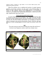
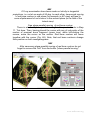
Setting of fragment markers according to mechanical axes
The blue angle is used for finding of mechanical axis of bone fragment.
It is located on one of centrators (Fig. 55). In this case centrator without the
blue angle must be ignored. It should be, using its central red point, moved
out of borders of bone fragment. On default the blue angle settles down to
the left of an axial line. If necessary it can be placed to the right of an axial
line. For this purpose overlap the cursor with left point of centrator and
press the left button of the mouse. While left-clicking the mouse, move this
point left-to-right. As result blue angle meets the right position (Fig. 60).
a
www.ortho-suv.org
76
b
Fig. 60. Indicator of angle of axial line positioning (blue angle). a - centrator without
blue angle must be moved out of bone fragment borders, so it is ignored. b - if
necessary blue angle can be arranged to the right of axial line. For this purpose overlap
cursor with left point of centrator and press the left button of the mouse. While leftclicking mouse, move this point left-to-right. As result blue angle meets the right position
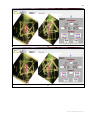
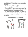
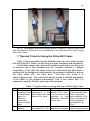
The mechanical axis (as well as an anatomic axis) is known to cross a
joint line in the certain point at the certain angle. Localization of crossing
and value of an angle are specific for proximal and distal joints of each long
bone in frontal and sagittal planes [Paley D., 2003; Solomin L.N., 2008,
2013]. With reference to Ortho-SUV software, centrator with blue angle is a
joint line. Thus, to find a mechanical axis of a bone fragment, the centrator
with blue angle must be placed in a projection of joint line. At the same time
the vertex of the blue angle must be placed at a due point of crossing of the
mechanical axis and the joint line. For this purpose red points of the
centrator is moved in a necessary direction. After that necessary value of
blue angle must be set. For this purpose there are fields “Blue angles on
AP view” and “Blue angles on Lat view” in Step 10.
For example, it is known, that the proximal tibial mechanical angle in
frontal plane is 87 deg., and the mechanical axis should cross the joint line
in its centre. Moving with the help of the left-mouse extreme red points of
the centrator, place the centrator to coincide with joint line and the vertex of
the blue angle must be located in the centre of the joint line. After that in
the field “Blue angle of base fragment marker” insert “87” and press the
button “Blue angle of base fragment marker”. The axial line will be placed
at an angle of 87 deg. to the centrator (joint line), designating the
mechanical axis of the proximal fragment (Fig. 61).
www.ortho-suv.org
77
a
b
Fig. 61. Finding mechanical axis of proximal tibial bone in frontal plane with help of
blue angle. a – diagram of mechanical angle. b – centrator with blue angle is placed on
joint line and vertex of blue angle coincides with centre of joint line. Due value of blue
angle 87 deg. is inserted. It leads to that axial line of green tree takes position of
mechanical axis of bone fragment. Note, that yellow point is placed on distal border of
proximal fragment
It is known, that the proximal femoral mechanical angle in frontal plane
is 90 deg., and the mechanical axis should cross the joint line in the centre
of femoral head. Moving with the help of the left-mouse extreme red points
of the centrator, place the centrator to coincide with joint line and the vertex
of the blue angle must be placed in the centre of femoral head. After that in
the field “Blue angle of base fragment marker” insert “90” and press the
button on “Blue angle of base fragment marker”. The axial line placed at an
angle of 90 deg. to the centrator (joint line), designating the mechanical
axis of proximal fragment (Fig. 62).
a
b
Fig. 62. Finding mechanical axis of proximal femoral bone in frontal plane with
help of blue angle. a – diagram of mechanical angle. b – centrator with blue angle is
placed on joint line and vertex of blue angle coincides with centre of femoral head. Due
www.ortho-suv.org
78
value of blue angle 90 deg. is inserted. It leads to that axial line of tree takes position
of mechanical axis of bone fragment. Note, that yellow point is placed on distal border of
proximal fragment
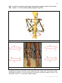
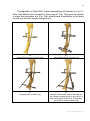
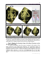
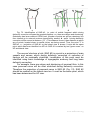
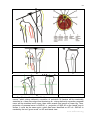
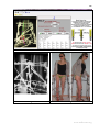
The Ortho-SUV software window in Step 10 at finding of mechanical
axes of femoral fragments in frontal plane with the use of blue angle is
shown in Fig. 63.
a
b
www.ortho-suv.org
79
c
Fig. 63. The Ortho-SUV software window in Step 10 at finding of mechanical axes
of femoral fragments in frontal plane with use of blue angle. a – centrator with blue
angle is placed on joint line and vertex of blue angle coincides with centre of femoral
head. Due value of blue angle 90 deg. is inserted in field “Blue angle of base fragment”.
It leads to that axial line of tree takes position of mechanical axis of bone fragment. b –
centrator with blue angle is placed on knee joint line and vertex of blue angle coincides
with centre of joint line. Due value of blue angle 88 deg. is inserted in field “Blue angle
of mobile fragment”. It leads to that axial line of violet tree takes position of mechanical
axis of mobile fragment. Yellow points are placed on borders of proximal and distal
fragments. For Lat view anatomic axes of fragments has been found with use of both
centrators. c - diagram of finding mechanical axes of fragments in frontal plane
Finding anatomic axes with the help of blue angle
When the length of a bone fragment does not allow using centrators to
find anatomic axis, the blue angle can be used.
The anatomic axis (as well as the mechanical axis) is known to cross a
joint line in the certain point at the certain angle. Localization of crossing
and value of an angle are specific for proximal and distal joints of each long
bone in frontal and sagittal planes (Paley D., 2003; Solomin L.N., 2008,
2013). With the reference to Ortho-SUV software, centrator with the blue
angle is a joint line. Thus, to define an anatomic axis of a bone fragment,
centrator with the blue angle must be placed in a projection of joint line. At
the same time the vertex of the blue angle must be placed at a due point of
crossing of the anatomic axis and the joint line. After that necessary value
of the blue angle must be set. For this purpose there are fields “Blue angles
on AP view” and “Blue angles on Lat view” in Step 10.
For example, there is a supracondylar deformation of a femur. The
length and the shape of distal fragment do not allow using the centrators.
For example, it is known, that the distal femoral anatomic angle in sagittal
www.ortho-suv.org
80
plane is 83 deg., and the anatomic axis should cross the joint line at its
anterior third. Moving with the help of the left-mouse extreme red points of
the centrator, place the centrator to coincide with joint line and the vertex of
the blue angle must be placed at the anterior third of the joint line. After that
in the field “Blue angle of mobile fragment marker” insert “83” and press the
button on “Blue angle of mobile fragment marker”. The axial line placed at
the angle 83 deg. to the centrator (joint line), designating the anatomic axis
of distal fragment (Fig. 64).
a
b
c
Fig. 64. Finding anatomic axis of distal femoral bone fragment in frontal plane with help of
blue angle. a – diagram of anatomic angle. b - as bone fragment is short, centrators can not be
used. Distal centrator is moved off border of distal fragment. Centrator with blue angle is placed
on joint line and vertex of blue angle coincides with anterior third of joint line. Due value of blue
angle 83 deg. is inserted. It leads to axial line of violet tree takes position of anatomic axis of
bone fragment. Yellow point is placed on proximal border of distal fragment. c - software
window at finding anatomic axes of femur in сsagittal plane. Anatomic axis of proximal fragment
is found with the help of centrators
www.ortho-suv.org
81
Having placed the bone fragment markers, click on the “Forward”
button to continue.
Step 11: Correction of the Final Position of the Mobile Fragment
After execution of Step 10 and clicking the "Fwd" button, in the field of
roentgenograms yellow bone contours appear again. Let's remind that
yellow bone contours are made in Step 8 and with their help the program
designates an initial position of a mobile fragment. In addition it Step 11 red
bone contours appear. By red bone contours the program designates final
position of a mobile fragment after deformity correction or fracture
reduction.
NB!
Yellow bone contours mean the initial position of the mobile fragment.
Red bone contours mean the final position of the mobile fragment.
To correctly estimate the position of red bone contours maximal
magnification must be used.
If in Step 11 bone contours are invisible, it is necessary to press the
right button of the mouse. It results in appearance of the pop-up menu. In
the pop-up menu it is necessary to chose “Visibility of bone fragment
contours” and to press the left button of the mouse. In addition, using this
pop-up menu is possible to make markers of bone fragments (green and
violet trees) visible, or, on the contrary, invisible. For this purpose the
button “Visibility of bone fragment markers” should be used (Fig. 65).
Fig. 65. Ortho-SUV program window in Step 11. There are bone fragment markers
(trees) and yellow and red bone contours in field of roentgenograms. Yellow bone
contours are initial position of mobile fragment; red bone contours are final mobile
www.ortho-suv.org
82
fragment position. Pressing of right button of the mouse leads pop-up menu
appearance (pointed by arrow)
When the software user is satisfied with position of mobile fragment
(position of red bone contours), he may pass to the following Step 12.
When red bone contours have not the proper position, it is possible to
correct it. The software options have capabilities to move red bone
contours by necessary value upwards and downwards, to the left and to the
right, angulate and rotate them as well.
Vertical and horizontal axial movings
To move red bone contours upwards, it is necessary to insert the value
of moving (in mm) and tick the window "Up". After that the red bone
contours on both roentgenograms will move upwards by the given value.
To move the red bone contours downwards, it is necessary to insert the
value of moving (in mm) and tick the window "Down". After that red bone
contours on both roentgenograms will move down by the given value (Fig.
66).
NB!
The axial moving up and down will take place along the axial lines of
the basic bone fragments markers (axial lines of green trees).
a
www.ortho-suv.org
83
b
c
www.ortho-suv.org
84
d
Fig. 66. Ortho-SUV program window in Step 11: vertical moving of red bone
contours. a - necessary value is inserted into field of vertical moving - 11 mm. b - tick
opposite "Up" is put. It has led to moving of red bone contours up. c - necessary value
is inserted into field of vertical moving - 15 mm. d - tick opposite "Down" is put. It has
led to moving of red bone contours downwards
To move red bone contour on the AP view to the left, it is necessary to
insert the value of moving (in mm) and put a tick in the window "Left". After
that red bone contour on the AP view will move to the left by the given
value (Fig. 67). To move red bone contour to the right, the tick should be
inserted in the window "Right". Red bone contour on the lateral view is
moved in a similar way. The field “Lat view” must be used.
www.ortho-suv.org
85
a
b
www.ortho-suv.org
86
c
d
Fig. 67. Ortho-SUV program window in Step 11: horizontal moving (translation) of
red bone contour. a - necessary value (11 mm) of translation is inserted into field “AP
view”. b - button “Left” is clicked. It has led to moving of red bone contour to the left on
AP view. Note, that "to the left" in this case means "inwards". c - necessary value (14
mm) of horizontal moving is inserted into field “Lat view”. d - button “Right” is clicked. It
has led to moving of red bone contour to the right on Lat view. Note, that "to the right" in
this case means "back"
www.ortho-suv.org
87
NB!
If X-ray examination have been made not strictly in tangential
projections, i.e. not at an angle of 90 deg. to each other, transversal moving
of red bone contour in one plane (for example, in AP view) will lead to
some displacement of red contour in the second plane (in the field of the
lateral view).
Free plane-parallel moving of red bone contour
There is a button "plane-parallel moving" in the panel of tools in Step
11. Tick here. Then, having placed the cursor with any of red points of the
marker of proximal bone fragment (green tree), while left-clicking the
mouse, move the cursor on the screen. Red bone contour will move
together with the cursor (Fig. 68). Note, that red bone contours change
their position on both roentgenograms.
NB!
After necessary plane-parallel moving of red bone contour do not
forget to remove the "tick" from the button "plane-parallel moving".
a
www.ortho-suv.org
88
b
c
Fig. 68. Ortho-SUV program window in Step 11: free plane-parallel moving of red
bone contour. a - button “plane-parallel moving” is ticked. The cursor is placed at one of
red points (any can be used) of proximal fragment marker – green tree (pointed by
arrow). b – while pressing left button of mouse red contour is moved to necessary
position. c - "tick" in the button “plane-parallel moving” is being removed
Red bone contour angulation
In Step 11 the fields “Angle 1” and “Angle 2” show the angles between
the axial lines of the basic and mobile bone fragments markers: “Angle 1”
for the AP view and “Angle 2” for the lateral view. These values can be
used as reference points for necessary turn (angulation) of red bone
contour.
www.ortho-suv.org
89
For red bone contour angulation any of red points of the proximal
bone fragment marker (green tree) can be used. It is most convenient to
use the red points which are placed on the axial line of green tree. Place
the cursor at any of these points and while keeping the left button of the
mouse pressed, move the cursor on the screen. Red bone contour will
move with the cursor together (Fig. 69). By experimentally changing points,
achieve necessary position of red bone contour.
Note, that red contours change the position on both roentgenograms.
a
b
www.ortho-suv.org
90
c
Fig. 69. Ortho-SUV program window in Step 11: red bone contour angulation. a cursor is placed at one red points (any can be used) of proximal bone fragment marker
(green tree) – pointed by arrow. b - while pressing left button of the mouse chosen red
point is being moved. It leads to angulation of red bone contour. c - by experimentally
changing red points necessary position for red bone contour is being achieved
Rotation
To rotate the mobile bone fragment (red bone contour) it is necessary
to insert necessary value of rotation into appropriate window. After that it is
necessary, using the left button of the mouse, to tick in the field: “Rotation
to the left” or “Rotation to the right” (Fig. 70).
a
www.ortho-suv.org
91
b
Fig. 70. Ortho-SUV program window in Step 11: rotation of mobile fragment. a –
value of necessary rotation, 20 deg., is being entered into field "Rotation" (specified by
arrow). b - field “rotation to the left” is being ticked. It has resulted to that the form and
the sizes of both red bone contours changed
NNB!
It is necessary to take into consideration, that the program calculates
moving of mobile bone fragment from an initial position to final one using
the shortest trajectory - directly from "point A" to "point B". Therefore at
overlapping of bone fragments it is necessary to execute reduction in two
stages. The first stage is distraction to achieve 3-4 mm gap between
fragments. The second stage is residual deformity correction. If not to do it,
fragments "will be linked" and reduction becomes impossible (Fig. 71).
www.ortho-suv.org
92
a
b
www.ortho-suv.org
93
c
Fig. 71. Software calculates moving of mobile fragment on the shortest trajectory "directly". a - moving on the shortest trajectory fragments will be linked and reduction
becomes impossible. b - at fragments overlapping it is necessary, at first stage, to
perform distraction to achieve 3-4 mm gap between fragments. c - after gap has
appeared total residual correction can be done
NB!
Before Step 12 position of the red bone contour must be controlled
using maximal magnification. A little residual displacement or possibility of
"linking" of bone fragments can not be noticed at small magnification.
If options “Plane-parallel moving” and (or) “Angulation” have been
used, the command “to confirm moving” (in the accepted slang - “to click
the pointer”) must be done before going to Step 12. To do this it is
necessary to place the cursor at the red point connected to the yellow point
(index of border of proximal bone fragment) in a lateral view and press the
left button of the mouse. After that confirm moving of mobile fragment by
clicking the pointer (Fig. 72).
www.ortho-suv.org
94
a
b
Fig. 72. Ortho-SUV program window in Step 11: performance of command “to
confirm moving” (“click pointer”). a - after having placed cursor at red point connected
with pointer of proximal fragment border (“yellow point”) (specified by arrow), left button
of the mouse must be pressed. b – the same “click pointer” procedure must be done for
mobile fragment (pointed by arrow)
NB!
Do not forget to execute the command “to confirm moving” (“click
pointer”).
If you are convinced of correct position of the mobile bone fragment
(i.e. red bone contour), press button "Fwd". If after pressing button “Fwd”
www.ortho-suv.org
95
an icon “Click the pointer” will appear, it is necessary to repeat procedure
“to confirm moving” (Fig. 72), using pointers not only in lateral view, but
also in AP view.
Step 12: Designation of “Structures at Risk”.
Performance of Step 12 allows the program to obtain the data for
calculation of necessary rate of deformity correction. The parameters given
are “Structures at Risk” (SAR).
The first structure at risk (SAR #1) is a point located on proximal edge
of mobile fragment which at deformity correction or reduction of fracture will
be moved by the maximal distance. Localization of this point must be
identified using basic knowledge of long bone deformity correction.
For example, there are valgus and shortening. In this case the point
which is located at osteotomy level in a projection of external cortex after
deformity correction will be moved at the greater distance, than any of the
points which are closer to internal cortex. This point must be designated, as
SAR #1 (Fig. 73). SAR #1 also must be marked in the lateral view. SAR #1
on the lateral view must be the same point, which was chosen for the AP
view (Fig. 73c,d).
NB!
SAR must be the same points for AP and lateral view.
a
b
www.ortho-suv.org
96
c
d
Fig. 73. Identification of SAR #1, i.e. point of mobile fragment which during
deformity correction will pass the greatest distance. a – there are valgus and shortening.
Osteotomy has been made at CORA level. Number of points are put on osteotomy line
from internal up to external cortexes (specified by arrows). b - point 1 during deformity
correction will be moved at distance (1-1’). This distance is more, than distance at which
any of points, located closer to medial cortex, are being moved. Thus, the point "1" is
SAR #1. c - projection of SAR #1 on the lateral view is shown. It must be the same
point, which has been identified on AP! d - SAR #1 is marked by tool “green cross” on
AP and lateral view
The second structure at risk (SAR #2) is a point in a projection of main
vessels and nerves, which during deformity correction or reduction of
fracture will be maximally stretched. Localization of this point must be
identified using basic knowledge of topographic anatomy and long bone
deformity correction.
For example, there are valgus and shortening of proximal tibia. In this
case peroneal nerve will be most stretched during deformity correction.
Therefore the projection of peroneal nerve is SAR #2 (Fig. 74). SAR #2
should be marked on the lateral view too. It must be the same point, which
has been determined for AP view.
www.ortho-suv.org
97
a
b
c
d
Fig. 74. Identification of SAR #2, i.e. point in projection of main vessels and
nerves, which during deformity correction or reduction of fracture will be maximally
stretched. a – there are valgus and shortening. b - during deformity correction peroneal
nerve will be stretched much more, than other vessels and nerves of lower leg. Thus,
projection of peroneal nerve is SAR #2. c - projection of SAR #2 on the lateral view is
shown. It must be the same point, which has been identified on AP! d - SAR #2 is
marked by the tool “green cross” on AP and lateral view
www.ortho-suv.org
98
There is a special tool for SAR designation: two intercrossing lines of
green color - “green cross”. Place the cursor at the centre of the green
cross on AP view. Than press the left button of the mouse and move the
green cross to the projection of SAR #1. The same way SAR #1 must be
marked on the lateral view. After that press the button “SAR #1”.
Next step is marking of SAR #2. To do this move the green cross in
projection of SAR #2 sequentially on AP and Lat view. Finally press the
button “SAR #2”. After that in the window “Distance between SAR” distance
between SAR in mm can be seen (Fig. 75).
When the orthopedic surgeon is convinced, that the stretching of main
vessels and nerves can be ignored, SAR #2 should not be designated. For
example, at segment lengthening the stretching of vessels, nerves and
length of regenerate will be equal. The other example is femur valgus
deformity correction, because the length of regenerate will exceed a
stretching of vessels and nerves. In similar cases after designation of SAR
#1, the button SAR #2 must immediately be pressed. After that in the
window “Distance between SAR” digit "0" will appear. For the program it
means that SAR #1 and SAR #2 coincide.
After SAR designation button "Fwd" must be pressed.
а
www.ortho-suv.org
99
b
с
Fig. 75. Ortho-SUV program window in Step 12: identification of structures at risk SAR. a - SAR #1 on AP and Lat view is marked by the tool “green cross”. It must be the
same point! After that button “SAR #1” is being pressed. b - SAR #2 on AP and Lat view
is marked by the tool “green cross”. It must be the same point! After that button “SAR
#2” is being pressed. In window “Distance between SAR” figure 44.9 has appeared. It is
distance between SAR in mm. c – it was decided to ignore SAR #2. For this purpose
after designation of SAR #1 button SAR #2 should immediately be pressed. After that in
the window “Distance between SAR” digit "0" has appeared. For the program it means
SAR #1 and SAR #2 coincide.
www.ortho-suv.org
100
Step 13: Strut Length Change
To define the rate of deformity correction (fracture reduction) a value
(in mm/day) is entered in the “Rate of correction” field (Fig. 76). The default
value is 1 mm/day but the user can enter any other value; the minimal
value is 0.1 mm/day.
Fig. 76. Ortho-SUV program window in Step 13: choice of rate of correction. The
deformity correction rate has been entered: 1 mm/day
Next, click the “Calculate” button; the program will calculate the
number of days required for the deformity correction at the given rate.
Result of calculation appears in a field “Recommended number of days”
(Fig. 77). Calculated by software number of days provides daily moving any
of SAR not more, than by value chosen, for example, 1 mm/day.
Note, that the user has a possibility to ignore the number of days
calculated by the program. Just remove it and enter the number of days
required.
There is another possibility to change number of days for deformity
correction. For this purpose it is necessary to change value in the field
“Rate of correction”, for example, 2.5 mm/day, and again (do not forget it!)
to press the button "Calculate".
www.ortho-suv.org
101
a
b
Fig. 77. Ortho-SUV program window in Step 13: identification numbers of days
needed for deformity correction. a - software has calculated recommended number of
days for deformity correction at rate 1 mm/day - 19 days. The user can ignore this
value. To do this just remove it and enter number of days required. b - there is another
possibility to change number of days for deformity correction. For this purpose it is
necessary to change value in the field “Rate of correction” for necessary one (for
example, 2.5 mm/day) and again (do not forget it!) press the button "Calculate". The
program has calculated, that at new rate 8 days are necessary for deformity correction
After that the user should specify at what rate lengths of strut can be
changed. The program gives a choice: once a day, twice a day and four
times a day. Having made a choice tick in an appropriate window: “Once a
www.ortho-suv.org
102
day”, " Twice a day" and "Four times a day". Right after tick has been
put, the help will appear to the right of the basic window (Fig. 78).
a
b
www.ortho-suv.org
103
c
Fig. 78. Ortho-SUV program window in Step 13: choice of number of strut change
lengths a day. Possible variants of choice and the helps given by the program are
shown
After that number of days and rate of correction have been identified,
the button “Show” must be pressed. After calculations the program will
show the table of values of daily change of strut lengths (Fig. 79). The first
column of the table shows number of days of deformity correction. Six next
columns show lengths each of struts. Rows of days are divided by rows of
time recommended for changing strut lengths.
www.ortho-suv.org
104
Fig. 79. Ortho-SUV program window in Step 13: table of deformity correction
protocol
The table, using button "Print", should be printed out and used in daily
control for deformity correction. The printed table contains the help (Fig.
80).
www.ortho-suv.org
105
a
www.ortho-suv.org
106
b
www.ortho-suv.org
107
c
Fig. 80. Printed table of deformity correction protocol. a-c - examples of tables
calculated for different rates of strut lengths change
www.ortho-suv.org
108
At end of work with the program (as well as after each Step) the file
must be saved using the standard button of the panel of tools. It is always
possible to return to this file for control and recalculation. The file opens
from the Step at which the program was closed.
NB!
At acute deformity correction sizes of those struts to be extended must be
firstly changed. Only after that the struts recommended by software should
be shortened (Fig. 81). It allows avoiding possible "interengage" of bone
fragments.
a
www.ortho-suv.org
109
b
Fig. 81. Ortho-SUV program window in Step 13 at acute deformity correction. a number "1" is entered into window “Recommended number of days”. b – there are three
rows in table: initial strut length (row “Day: 0”), final strut length (row “Day: 1”) and
between them row "12AM" – number of clicks needed for change of strut length. First
length of struts ## 1, 3 and 5 should be changed, because they are lengthened. Only
after that it is necessary to shorten struts ## 2, 4 and 6.
NB!
If for some reason difficulties have occurred (usually associated with
incorrect usage), save the file, archive the case folder (AP, Lat view, and
"**.suv"-file) and send it to the following email address:
[email protected] . In the accompanying message, explain in detail the
problem that has been encountered. To resume working, it is usually
enough to re-start the program and, obviously, avoid one’s previous
mistakes.
6. Application of Ortho-SUV Frame: Clinical Cases
6.1 Application of Ortho-SUV Frame in fracture treatment
22 y.o. patient В. was hospitalized with the diagnose: malunited midshaft
fracture of the left tibia with shortening, translation, and angulation of bone
fragments (Fig. 82а).
www.ortho-suv.org
110
External fixation of left lower leg using an Ortho-SUV Frame has been
performed. Wires were inserted in a way, that not to interfere with consequent
nailing (Fig. 82b):
Method of the Unified Designation of External Fixation (MUDEF):
I,9-3; II,9-3 _ IV,3-9 _ Ortho-SUV _ IV,3-9 _ IX (8-2)IX,8-2; IX,4-10
2/3 140
140
140
140
An attempt of close reduction in «fast struts» provided an improvement of
bone fragment position (Fig. 82с). Ortho-SUV software was used to calculate
elimination of residual displacement (Fig. 82d). Bone fragment reduction
carried out within 10 days (Fig. 82e). After that nailing was executed (Fig.
82f,g).
a
www.ortho-suv.org
111
b
c
d
www.ortho-suv.org
112
e
f
g
Fig. 82. Photographs and roentgenograms of patient В.
6.2 Application of Ortho-SUV Frame in diaphyseal deformities.
6.2.1 Both lower legs non-unions accompanied with complex deformities
45 y.o. patient Е., was hospitalized with the diagnose: nonunions of distal
third in both tibias. Complex six-component, three-planar deformity of right
lower leg. Complex five-component, two-planar deformity of left lower leg (Fig.
83а).
At the first stage, combined external fixation of bones in both lower legs
was performed using Ortho-SUV Frame (Fig. 83b).
For the right leg:
www.ortho-suv.org
113
III,12,100; IV,10-4; V,2,80
VIII,1,90
_ Ortho-SUV _
150
VI,12,90; VII(8-2)8-2;
150
For the left leg:
IV,12,100; V,10-4; VI,2,80 _ Ortho-SUV _ VII,12,90; VIII(8-2)8-2; VIII,4-10
150
150
The computer program was sequentially used for the right and left
lower legs. Fragment markers were set over projections of anatomical axes
of the bone fragments (Fig. 83с).
The rate of deformity correction was found by software in Step 12
according to SAR points. SAR #1 was set along the nonunion line, in the
place where the mobile fragment in the process of its transport will cover
the longest distance (Fig. 83d). SAR #2 was set in projection of main
vessels and nerves (Fig. 83e).
In Step 12 the rate of deformity correction - 1 mm per day – was
entered. After “Calculate” button was pressed, program calculated the
recommended number of days required for correction of the deformity.
When button «Show» had been pressed, in the lower right field of the
display a table appeared displaying the values of daily length change for
each strut (Fig. 83f). This table was printed out and given to the patient.
Calculation for deformity correction of the left lower leg was executed
in the same way.
Deformity correction was performed according to the calculations made
(Fig. 83g). Second stage involved nailing of both lower legs (Fig. 83h).
In 1.5 year after the surgery the locking nails were removed (Fig. 83i).
a
www.ortho-suv.org
114
b
c
www.ortho-suv.org
115
d
e
f
www.ortho-suv.org
116
g
h
i
Fig. 83. Photographs and roentgenograms of patient Е. before, during and after
the treatment
www.ortho-suv.org
117
6.2.2 Femur shaft deformity correction
28 y.o. patient K. was hospitalized with the diagnosis: Posttraumatic
complex two-level deformation of the right femur with shortening 4 cm (Fig.
84a).
The patient was operated: two-level osteotomy with applying two
Ortho-SUV Frames (Fig. 84b):
I,10,90; I,8,90 _ II,9,90; III,10,90
¼ 200
2/3 220
_ O-SUV _ IV,9,90; V,10,90 _ O-SUV _ VII,9,90;VIII,3-9; VIII,8,90; VIII,4,90
200
180
In calculation bone fragment markers were drawn in a projection of
anatomic axes of bone fragments. Calculations were made separately for
each of levels of deformation (Fig. 84c).
To find time necessary for deformity correction, Structures at Risk
(SAR) were designated in Step 12.
Deformity correction was performed and the correct position of
mechanical axis of femur restored according to the software calculations
(Fig. 84f).
After deformity correction struts were replaced for Ilizarov hinges (Fig.
84g).
In 2 months after the beginning of the fixation period module
transformation of the device was executed (Fig. 84h).
In 130 days after the beginning of the fixation period the frame was
removed (Fig. 84i).
a
www.ortho-suv.org
118
b
c
www.ortho-suv.org
119
d
e
www.ortho-suv.org
120
f
g
www.ortho-suv.org
121
h
i
Fig. 84. Photographs and roentgenograms of patient Е. Before, during and after
treatment
6.3 Application of Ortho-SUV Frame in metaphyseal deformity
19 y.o. women K. was hospitalized with the diagnosis: distal
metaepiphyseal nonunion of the right tibia. Four-component, three-planar
www.ortho-suv.org
122
deformity of the right lower leg (Fig. 85а). United left femur fracture, treated
by external fixation device.
As the first stage external fixation using Ortho-SUV Frame was done
(Fig. 85 b,c):
I,9-3; I,4-10; II,1,90 _ IV,10-4; V,2,90 _ Ortho-SUV _
150
_
150
VII(8-2)8-2; VIII,4-10 _ calc., 8-2; calc.,4 -10; m/tars.,V- m/tars.,I
150
horseshoe-shaped support
While working with computer program basic fragment markers using
centrators were drawn in projection of anatomical axes of proximal
fragment on AP and lateral views. It was not difficult because of large size
of this fragment.
It was not possible to use centrators due to the shortness of distal
fragment (35 mm). To identify anatomic axes the “blue angle” was used.
Positions of crossing points of ankle joint lines and anatomic axes for AP
and lateral view are known (Paley D., 2005). In Step 10 the centrator with
blue angle was placed on the joint line in a way that apex of the blue angle
was localized in the centre of joint line. After that, using options of the
program, necessary value of blue angle was set: 89 deg. for the AP and
80deg. - for lateral view. As a result the axial line of the bone fragment
marker corresponded to anatomic axis of distal fragment (Fig. 85d,е).
To find time necessary for deformity correction, Structures at Risk
(SAR) were designated.
SAR #1 was put on the osteotomy line, at where the mobile fragment
during its movement will cover the longest distance (Fig. 85f). SAR #2 was
put in the projection at where main vessels and nerves will get its maximal
stretching (Fig. 85g).
In Step 12 the rate of deformity correction - 1 mm per day – was
entered. After “Calculate” button was pressed, program calculated the
recommended number of days required for correction of the deformity.
When button «Show» had been pressed, in the lower right field of the
display a table appeared displaying the values of daily length change for
each strut (Fig. 85h). This table was printed out and given to the patient.
Deformity correction was done according to software calculation (Fig.
85i). After deformity correction struts were replaced for Ilizarov hinges (Fig.
85j). The second stage was bone grafting of non-union site and corticotomy
for lower leg lengthening at level II (Fig. 85k).
The frame was removed in 207 days after bone grafting (Fig. 85l).
www.ortho-suv.org
123
a
b
c
www.ortho-suv.org
124
d
e
www.ortho-suv.org
125
f
g
www.ortho-suv.org
126
h
i
j
www.ortho-suv.org
127
k
l
Fig. 85. Photographs and photoroentgenograms of patient К. a - before treatment.
b,c - after Ortho-SUV Frame applying. d – arrows point at dialog box fields where
values of epimetaphyseal (anatomic) angles have been entered. e – arrows point at
blue angles. Because due value of blue angles were entered, axial lines of bone
fragment markers are located precisely in projection of anatomic axes of distal fragment
in frontal and sagittal planes. f,g – identification of structures at risk: SAR #1 and SAR
#2. h - results of software calculation. i-k - result of correction. l - result of treatment
6.4 Application of Ortho-SUV Frame in Foot Deformity Correction
19 y.o. women Z. was hospitalized with the diagnosis: complex deformity
of right foot with 5 cm shortening (Fig. 86а).
At first stage, V-shaped foot osteotomy and applying of two Ortho-SUV
Frames was done (Fig. 86b):
www.ortho-suv.org
128
120
_ VII 11,110; VIII,4-10; VIII,8-2(8-2) –Ortho-SUV– calc.4-10; calc.8-2 –0–
120
2/3 110
–0– tars.4-10; tars.8-2 –Ortho-SUV– m/tars.I- m/tars.II; m/tars.V- m/tars.III -- _____
120
120
120
Free (without transosseous elements) proximal and distal rings were
used to facilitate of struts fixation.
Calculations were done separately for each frame. The first frame and
the first calculation were used for hindfoot deformity correction (Fig. 86с).
The second device and the second calculation were used for midfoot
deformity correction (Fig. 86d).
Correction of deformation was executed precisely according to
calculations (Fig. 86e). After deformity correction frame module
transformation was done: struts were substituted for Ilizarov hinges and
free supports were removed (Fig. 86f). Final configuration of the device is:
VII 11,110; VIII,4-10; VIII,8-2(8-2) –o– calc.4-10; calc.8-2 –o–
120
2/3 110
–o– tars.4-10; tars.8-2 –o– m/tars.I- m/tars.II; m/tars.V- m/tars.III
120
120
The period of fixation lasted 4 months. In 6.5 months after operation
frame was demounted (Fig. 86g).
www.ortho-suv.org
129
a
b
www.ortho-suv.org
130
c
d
e
www.ortho-suv.org
131
f
g
Fig. 86. Photographs and photoroentgenograms of patient Z. before, during and
after the treatment
www.ortho-suv.org
132
6.5 Application of Ortho-SUV Frame in Treatment of Knee Joint
Stiffness
48 y.o. women P. was hospitalized with the diagnosis: consolidated
fracture of left femur, severe extension stiffness of left knee joint (15/0/0) (Fig.
87a).
Judet procedure was performed followed by Ortho-SUV Frame
application (Fig. 87b):
III,10,90; IV,8,90
¼ 200
– III,4-10; IV,1,80
150
VII,3-9; VII,8,90 –Ortho-SUV–
180
VIII(8-2)8-2; VIII, 4-10
150
While performing program calculations, to identify the motion curve of the
joint end of tibia relatively to femur, the Iwaki’s knee joint motions kinematics
was used [Iwaki H., 2000]. Proceeding from these calculations, knee joint
flexion up to 90 degrees was completed in 12 days (Fig. 87c,d). The cycle “90
deg. flexion – knee zero position” was then performed, using Ortho-SUV
Frame, twice a day during the following 5 days – ten cycles in all. Then struts
were removed and the patient performed active motions in knee joint (Fig.
87e). After that the external fixation device was removed. In remote period the
ROM in knee joint was 90/0/0 (Fig. 87f).
a
www.ortho-suv.org
133
b
c
www.ortho-suv.org
134
d
e
www.ortho-suv.org
135
f
Fig. 87. Photographs and photoroentgenograms of patient P. before, during, and
after the treatment. Note the correct interrelations in the knee joint during flexion using
Ortho-SUV Frame
7. Tips and Tricks for Using the Ortho-SUV Frame
Table 1 lists the possible specific difficulties that can occur while working
with the Ortho-SUV Frame, as well as tips for their avoidance and elimination.
As the table makes clear, almost all possible complications are the result
of incorrect use of the hardware and (or) software. However, if despite
consultation of the table the cause cannot be determined and difficulties in
working with the program are experienced, the operator is advised to archive
the case folder (AP, Lat view, and "**.suv"-file) and e-mail it to
[email protected]. The cover letter should include a detailed explanation
of the nature of the problem encountered. This is one reason why it is
essential to save the file after each step of the program.
Table 1. Complications occurring with use of Ortho-SUV Frame
#
1
2
Complications
During
assembly of the
external fixation
frame, it is
difficult to
connect the
struts with each
other.
Due to the short
distance
Main causes
The
initial
arrangement of the
struts differs from that
shown in Fig. 14a,b .
Prophylaxis
Arrange the struts as
shown in Fig. 14a,b .
It is necessary to use
algorithm of strut
assembly, submitted
at Fig. 21a-i.
Elimination
Prior to the assembly
of the external fixation
frame, arrange the
struts as shown in Fig.
14a,b. Use algorithm
of strut assembly,
submitted at Fig.
21a-i.
The distance between 1.
The
distance 1. Partial reassembly
the supports is <120– between the supports, of the external fixation
www.ortho-suv.org
136
between
the 150 mm.
basic supports,
it is difficult or
impossible
to
arrange
the
struts.
3
4
5
6
7
Loading the AP
image (Step 2)
does not result
in
its
appearance in
the
program
window.
During
reloading of the
file (with all
steps of the
program
previously
completed), at
Step 3, the
previously
loaded
roentgenogram
s are not visible.
It is not possible
to define the
number of
struts and joints
necessary and
thus to proceed
to the next step
on the X-ray
image (Steps 6
and 7); it is
difficult to define
the numbers of
struts and
joints.
In spite of all
struts and joints
having
been
marked in Step
6 or 7, the
program does
not
allow
continuation to
the next step.
After Step 7 has
if possible, must not
be <150 mm.
2.
Use
Z-shaped
plates to fix the struts
(Figs. 15c, 17b)
3. Use stabilizing
supports to fix the
struts (Fig. 17c,d)
A feature of the
program is that both
roentgenograms
appear only after the
second, lateral one
has been loaded.
This is a feature of the
program: you will be
able to work with the
images on all of the
following steps.
-
1. The X-rays are
made on narrow film
and do not include all
struts and joints.
2. The images were
obtained without the
use of strut markers
(Fig. 32 ).
1. The X-ray field
must include all struts
and joints.
frame
2. Strut fixation of
using Z-shaped plates
(Figs. 15c, 17b)
3. Fixation of some of
the struts to the
stabilizing
supports
(Fig. 17c,d)
-
-
X-rays
retaken
must
be
2. Strut markers must
be placed on the
struts prior
to X-ray imaging (Fig.
32 ).
The focal distance Entering all the data Enter
the
focal
and (or) the center of required
in
this distance
and
the
the beam value was window
beam center
not entered.
1. Incorrect assembly
1. Correct assembly of 1. Partial re-assembly
www.ortho-suv.org
137
been
completed, the
program shows
red lines that do
not
coincide with
the strut
projections s,
ranging from
the noncoincidence of
one of the lines
to the total
displacement of
all
lines relating to
the external
fixation frame.
In the extreme
case, the red
lines are
beyond the
visible field.
of the external fixation
frame: first of all, lack
of adherence to the
“logo rule” (Fig. 18)
and the “watch rule”
(Fig. 19).
2. Incorrectly entered
lengths of the struts
and sides of the
triangles or entry of
the values in cm (Step
1).
3. Incorrect scaling
(Steps 4, 5): the
length of the known
section is <80 mm
and (or) the length of
the known section
was entered in cm.
4. Incorrectly entered
focal distance (Steps
6, 7) or the focal
distance was entered
in cm.
5. Incorrectly marked
numbers of the struts
and (or) joints, i.e.,
lack of
correspondence to the
assembly of the
external fixation frame
(Steps 6, 7).
6. Coincidence of the
red lines with the
projections of the
struts depends on the
exact and correct
completion of Steps
1–7.
8
In advancing to
Step 10, the
program shows
a dialog window
1. Different lengths of
the bone contours
(Step 8) of the mobile
bone fragment on the
the external fixation of the external fi xation
frame
frame, which requires
an
additional
X-ray
image.
2. Exactly entered
values of the lengths
of the struts and sides 2. Exact lengths of the
of the triangles in
struts and sides of the
mm.
triangles are entered
in mm.
3. Exact value of the
known section length
3. Exact length of the
entered in mm.
known section entered
in mm.
4. Exact value of the
focal distance entered 4. Exact focal distance
in mm.
entered in mm.
5. Marking the
numbers of the struts
numbers and (or)
joints according to the
assembly of the
external fixation frame
by using the strut
markers when
obtaining an X-ray
image (Fig. 32).
6. Control of whether
the values have been
entered correctly in
the completion of
Steps 1–7. If the AP
and
lateral
roentgenograms were
not
taken
in
orthogonal
projections, then on
Steps 6 and 7 the
maximal
possible
number of struts and
joints
must
be
marked.
1. The lengths of the
bone contours on the
AP and lateral views
must be equal.
5.
Entering
the
numbers of the struts
and joints according to
the assembly of the
external
fixation
frame.
6. Thorough control of
the data entered in
Steps 1–7. Return to
Steps 6 and 7 and
mark the maximally
possible number of
struts and joints.
1. Erase the bone
contours and draw
them again, this time
of equal length.
www.ortho-suv.org
138
“Precise
the AP and lateral views.
anatomical
2. The anatomic axes
axes sizes.”
(Step 9) of the mobile
bone fragment on the
AP and (or) lateral
views
do
not
sufficiently exceed the
upper
or
lower
margins of the bone
contour.
9
When moving
from Step 11 to
Step
12
program shows
a
dialogue
window
“Improper
data”.
In the field "Rotation"
direction
and(or)
value of rotation were
not specified.
10
When moving
from Step 11 to
Step
12
program shows
a
dialogue
window “Click
both pointers”.
The button “planeparallel moving” has
been clicked (Fig. 68)
and(or) the command
“to confirm moving”
(“click pointers”) has
not been executed
(Fig. 72).
11
After the
“Calculate”
button has been
clicked to
calculate the
number of days
required for the
deformity
correction or
fracture
To calculate the
number of days
required for the
deformity correction or
fracture reduction, the
program always uses
the structures at risk
points (Figs. 73, 74
and 75). If these have
not been set, the
2. The anatomic axes
must exceed the
margins of the bone
contours by 20–30
mm.
2. I f it is impossible
to draw the anatomic
axis above the distal
end of the bone
contour (short X-ray
image). return to
Step 8, erase the
bone contour, and
draw a new one,
which must be
shorter than the initial
bone contour.
Any numerical value
of rotation must be
entered into the field
of value of rotation. In
addition
either
window, indicating a
direction of mobile
fragment
rotation,
must be ticked. If
rotation
is
not
required, "0" (zero)
and any direction of
rotation
must
be
entered.
If options “Planeparallel moving” and
(or)
“Angulation”
have been used, the
command “to confirm
moving”
(“click
pointers”) must be
done before going to
Step 12 (Fig. 68).
The button “planeparallel moving” must
not be clicked (Fig.
72).
Do not forget to
exactly locate both
structures
at
risk
points (Step 12 ).
It is necessary to
enter
value
of
rotation
and
its
direction.
Switch off the button
“plane-parallel
moving” (Fig. 68) and
execute
the
command “to confirm
moving”
(“click
pointers”) (Fig. 72).
Return to Step 11 and
exactly
set
the
structures
at
risk
points (Figs. 73, 74
and 75 ).
www.ortho-suv.org
139
12
13
14
reduction (Step
13), the
program
gives an
obviously
incorrect result:
for
example,
17
days for a 5mm distraction.
During
deformity
correction, the
struts begin to
press on the
soft tissues or
on the
outstanding
ends of the halfpins.
In a maximal
distraction
during
correction of the
deformity, the
threaded
rod
(Fig. 7) has
completely
dislocated itself
from the strut
length changing
unit (Fig. 9);
disconnection
of the unit and
the
threaded
rod
has
occurred, thus
destabilizing the
external fixation
frame.
On the control
X-ray image, an
exact deformity
correction not
shown;
the
location of the
distal fragment
does not fully
correlate
with
that of the red
bone
contour
program considers the
default settings for
these structures,
which cannot be
applicable to the
target case.
Incorrect
initial During
surgery Partial re-assembly of
assembly
of
the planning, it is essential the external fixation
external fixation frame to
consider
the frame
direction in which the
distal main support
and struts will be
moved.
There is no thread on
one of the ends of the
threaded rods packed
in the Ortho-SUV
Frame set, which
precludes
disconnection of the
strut length changing
unit and the threaded
rod.
If
this
complication
has
occurred, the rods
being used in the
external fixation frame
assembly
do
not
belong to the OrthoSUV set.
1. Use only the
threaded rods packed
in the Ortho-SUV set.
2. The threaded bush
of the strut length
changing unit (Fig. 9)
has a slot. It can be
used to control the
position
of
the
peripheral end of the
threaded rod.
Partial re-assembly of
the external fixation
frame, replacing the
threaded rod by a
longer one.
1. The location of the
distal fragment was
set by the user in Step
11:
therefore,
at
maximal
magnification,
examine the location
of the red bone
contour relative to the
basic
(proximal)
fragment.
1. The yellow bone
contour (Step 8) must
exactly coincide with
the contours of the
mobile bone fragment.
In
completing
deformity correction or
fracture
reduction
planning (Step 11),
the location of the red
bone contour of the
1. Additional program
calculation
and
elimination of the
residual displacement
www.ortho-suv.org
140
(Step 11).
2. Unstable fixation of
the bone fragments by
the proximal and (or)
distal external fixation
unit. As a rule, the
bone fragment relating
to
the
support
becomes
displaced
due to the deformity of
the
transosseous
elements.
proximal
fragment
must
be
visually
controlled
using
maximal
magnification.
2. Fixation of the
proximal and distal
bone
fragments must be
stable and exclude the
possibility of fragment
displacement relative
to
the
appropriate
supports.
3. X-ray projections
taken before and after
the
deformity 3. Take X-rays in the
correction do not same views
coincide.
15
16
The control Xray
image
shows that the
fragments have
interconnected,
which prevents
fracture
reduction
or
deformity
correction.
Thus,
further
changes in strut
length will result
in
the
deformation of
not only the
bone fragments
but of the whole
external
fixation frame
as well.
After the work is
complete
the
program does
not shut down
Note that the program
calculates the integral
trajectory for the bone
fragment
reduction,
i.e., according to the
shortest
distance.
Thus, if there is axial
displacement of the
bone fragments (the
proximal end of the
distal fragment is
higher than the distal
end of the proximal
fragment)
and
attempts are made to
eliminate
the
translation,
the
fragments will become
inevitably
interconnected.
If the proximal end of
the distal fragment is
higher than the distal
end of the proximal
fragment,
deformity
correction
(fracture
reduction) must be
performed in two
stages: (1) distraction
to provide
a 3–4 mm diastasis
between the bone
fragments (program
calculation planned for
distraction);
(2)
residual displacement
is eliminated (the
second
calculation
in
the
program) (Fig. 71).
The hasp-key was First shut down the
removed before the program and only
program was shut after that remove the
down.
hasp- key.
2. Reassembly of the
external fixation frame
(stabilizing
the
supports),
repeated
calculation
in
the
program
and
elimination of the
residual displacement
3.
Control
X-ray
images are obtained
in views different from
those that
enabled the detection
of
the
additional
displacement of the
fragments. Perform an
additional calculation
in the program and
eliminate the residual
displacement.
The first stage is
distraction to achieve
3-4 mm gap between
fragments.
The
second
stage
is
residual
deformity
correction (Fig. 71).
Insert the hasp-key in
to the USB-port and
after that shut down
the program.
www.ortho-suv.org
141
8. Instead of the conclusion
8.1. Legalization
Ortho-SUV Frame is patented and certified. All rights are reserved.
Copyright, Patent, and License infringement will be punishable by the fullest
extent of the Russian Federation laws.
For any questions concerning copyright and license agreement
registration apply to:
“Ortho-SUV” Ltd. (executive director – Victor Vilensky)
Vedeneeva Str. 8-1-282, St.-Petersburg, 195269, Russia
Tel. number: +7-921-316-3703
http://ortho-suv.org
E-mail: [email protected]
8.2. Ortho-SUV Frame training courses and workshops
Complete information concerning training courses for the Ortho-SUV
Frame can be found at http://ortho-suv.org, http://rniito.org/solomin,
http://www.rniito.org/download/ortho-suv-Iliz-course-9-engl.pdf
and
http://www.rniito.org/download/ortho-suv-course-4-eng.pdf .
To the attention of scientists and orthopedic surgeons
We invite you to take part in scientific and practical work, associated with
the Ortho-SUV Frame application and improvement. Further information can
be send to Prof. Leonid N. Solomin: Vreden Russian Research Institute of
Traumatology
and
Orthopedics;
[email protected],
http://rniito.org/solomin
8.3. Where to acquire
All information can be taken at web-sites of Ortho-SUV Ltd. and S.H.
Pitkar Orthotools Pvt. Ltd:
http://pitkar.com
http://ortho-suv.org
www.ortho-suv.org
142
9. References
1. Bonev I. (2003) The true origins of parallel robots copyright.
http://www.parallemic.org/Reviews/Review007p.html. - Accessed on Aug 25, 2005.
2. Dammerer D., Kirschbichler K., Donnan L., Kaufmann G., Krismer M.,
Biedermann R. Clinical value of the Taylor Spatial Frame: a comparison with the
Ilizarov and Orthofix fixators J Child Orthop (2011) 5:343–349.
3. Iwaki H, Pinskerova FMAR (2000) Tibiofemoral movement 1: the shapes and
relative movements of the femur and tibia in the unloaded cadaver knee. J. Bone
Joint Surg. 82-B:1189–1195
4. Marangoz S., Feldman D.S., Sala D.A., Hyman J.E., Vitale M.G. Femoral
deformity correction in children and young adults using Taylor spatial frame. Clin
Orthop Relat Res. 2008;466(12):3018–3024.
5. Method of Unified Designation of External Fixation (MUDEF). Available at:
http://orthosuv.org/index.php?option=com_content&view=article&id=127&Itemid=93&lang=e
n and http://ortho-suv.org. Accessed on October 23, 2012.
6. Paley D. (2005) Principles of deformity correction. Springer, New York
7. Paley D. (2011) History and science behind the six-axis correction external fi xation
devices in orthopaedic surgery oper Tech Orthop 21:125–128. Elsevier Inc.
8. Rozbruch S.R. Correction of tibial deformity with use of the Ilizarov-Taylor spatial
frame / S.R. Rozbruch, A.T. Fragomen, S.Ilizarov // J. Bone Joint Surg. – 2006. –
Vol. 88-A, Suppl. 4. – P. 156–174.
9. Seide K., Wolter D., Kortmann HR (1999) Fracture reduction and deformity
correction with the hexapod Ilizarov fixator. Clin Orthop 363:186–195
10. Seide K. (2004) Application of the Hexapod- fixator. Litos, Hamburg
11. Seide K., Gerlach U., Inden Ph., Bohn B., Juergens Ch. (2008) Dimensional
corrections with the Hexapod system added to the Ilizarov apparatus. In: 5th
meeting of the A.S.A.M.I. international: program and abstract book, St.
Petersburg, 2008, pp 83–84
12. Solomin, L.N. The basic principles of external fixation using Ilizarov device / L.N.
Solomin
//
Italy,
Milan:
Springer-Verlag,
2008.
–
357
p.
(http://rniito.org/solomin_eng/download/the_basics.pdf)
13. Solomin, L.N. Practical Classification of long bone deformities / L.N. Solomin, V.A.
Vilensky // 5th Meeting of the ASAMI International. Program and Abstract Book. –
St.Petersburg, 2008. – P. 339. (http://rniito.org/solomin_eng/deform_class.jpg)
14. Solomin L.N., Terrell W., Odessky J. (2008) Multifactorial comparative analysis of
Ilizarov apparatus and external fixation devices on the base of computer
navigation (Taylor Spatial Frame, Ilizarov Hexapod Apparatus, SUV-Frame). In:
5th meeting of the ASAMI international. Program and abstract book. St.
Petersburg, 2008, p 52
15. Solomin, L.N. Comparative analysis of reduction capabilities provided by software
based external fixation devices and Ilizarov apparatus / L.N. Solomin, V.A. Vilensky,
A.I. Utekhin, W. Terrell // The Genius of Orthopedics. – Kurgan, 2009. - # 1 – 5-10
p.p.
16. Solomin, L.N. Comparative analysis of reduction capabilities provided by software
based external fixation devices and Ilizarov apparatus / L.N. Solomin, V.A. Vilensky,
www.ortho-suv.org
143
A.I. Utekhin, W. Terrell // The Genius of Orthopedics. – Kurgan, 2009. - # 1 – 510 p.p.
17. Solomin, L.N. Comparative analysis of rigidity fixation provided by software based
external fixation devices and Ilizarov apparatus / L.N. Solomin, V.A. Vilensky, A.I.
Utekhin, W. Terrell // Traumatology and Orthopedy of Russia. – St.-Petersburg,
2009. - # 2. – 20-25 p.p.
18. Solomin L. (2013) The basic principles of external skeletal fixation using the
Ilizarov and other devices. Springer, Milan
19. Solomin L., Vilensky V., Utekhin A. Deformity Сorrection and Fracture Treatment
by Software-based Ortho-SUV Frame: User Manual. Available at: http://orthosuv.org. Accessed on March 12, 2013.
20. Taylor J.C. (1997) A new look at deformity correction. Distraction. The Newsletter
of ASAMI-North America 5(1)
www.ortho-suv.org
144
Appendix 1
Steps to be followed before you start using the Ortho-SUV Frame Software
Step No. 1
Create a folder named Ortho-SUV on your Laptop / Desktop, on which you want to run the program.
Step No. 2
Insert the Ortho-SUV Frame Software CD supplied to you in the disk drive of your Laptop / Desktop.
Copy the folder SUV-Software on the software CD into the Ortho-SUV Folder created by you.
Step No. 3
Click on the “Hasp” folder, then click on the folder “Sentinel_LDK_Run-time_setup-2011” & click again
on “HaspUserSetup.exe” file. Install the Hasp program following the steps as prompted.
Step No. 4
Before working in the program it’s necessary to create the folder for the clinical case. In this folder AP
and lateral x-ray images of the patients in (jpeg) or (.bmp)format should be placed. In the same folder
the file made later by Ortho-SUV program for the subject case should be also saved.
Step No. 5
Attach the Hasp key to the USB drive of your laptop & then double-click “SUV-Software.exe” file.
Program window will appear. Press the "New document" button. Save your case folder allocating a file
name to it & then follow the steps as prompted by the software.
Note 1: Immediately after the new document (that is, “clinical case”) has been created, it is necessary to
save it (command “Save” in “File” menu) in the patient case folder. It is recommendable to repeat saving
after every step.
Note 2: The software will not work without the Hasp Key. Hence, ensure that the Hasp key is kept safely.
www.ortho-suv.org