Download FLAC - Itasca Denver, Inc.

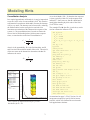
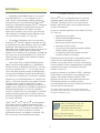
Soft Spot
Itasca’s Software Newsletter
In the Spotlight
W
ith the release of
FLAC3D Version 2.0,
Itasca begins offering
Windows 95 and Windows
NT versions of its software.
Over the next 18 months, we
plan to develop Windows*
versions of FLAC and PFC.
(See page 2 for details.)
We believe that this
development will not only
allow us to include more
user-friendly features, but it
also provides the facility to
add different solution schemes
(including parallel processing)
to improve the calculation
speed. We are very excited
about the potential of this new
software development.
We’ll keep you informed of
our progress in future issues.
VOLUME 5 number 1
JUNE 1997
FLAC 3D Version 2.0 is Now Available
e are pleased to announce the release of the latest version of
FLAC3D. Version 2.0 is provided as both a DOS application and a
native Windows* application that can operate in Windows 95 or
Windows NT. Users can now access the facilities available to Windows
applications, such as input/output control, multitasking and graphical utilities.
Save files are compatible between the DOS and Windows versions, so models
can be created in the Windows version and solved in the DOS version, to take
advantage of the faster calculation speed available in DOS.
W
Shell elements are now available as part of the expanded structural element
logic in FLAC3D. Four types of structural elements are provided: beam, cable,
pile and shell. Beams, cables, and piles are two-noded linear elements; shells
are three-noded triangular elements. All elements interact with the FLAC3D
grid at their nodes; the particular type of interaction differs depending on
element type. The figure below shows a model for an advancing tunnel
excavation supported by steel (cable) bolts and a shotcrete (shell) lining.
(Turn to FLAC3D Version 2.0 on page 8)
* WindowsTM is a trademark of Microsoft Corporation.
— Roger Hart,
Director of Software Services
Inside
Under Development . . . . 2
Modeling Hints. . . . . . . . 3
Consolidation Analysis . . . . 3
Modeling an Embedded
Retaining Wall . . . . . . . . . . 4
User-defined Joint Models
in UDEC . . . . . . . . . . . . . . . 6
FISH Library Update . . . 6
Questions & Answers. . . 7
Soft Notes . . . . . . . . . . . . 8
Axial stress in steel bolts and bending moments in shotcrete lining at a tunnel
intersection
Under Development
There are three ongoing major software
developments. Please contact us if you wish to
receive additional information on any of these
developments.
FLAC++ — A native Windows 95 / NT version of FLAC is
presently under development. FLAC++, written in C++, will
overcome many of the restrictions of FORTRAN-based FLAC,
including the following:
1. FLAC++ will have double-precision variables in all
important calculation modules. This will provide more
accurate solutions for problems involving small
incremental changes over long time periods, such as
transient groundwater and creep simulations.
FLAC Version 3.4 — Several new features will
be available in our next release of FLAC:
• an option for high resolution graphics,
• user’s manual on CD-ROM,
• generalized ATTACH logic for grids of
•
•
•
•
•
•
2. FLAC++ will include a general x,y-grid specification as
well as the existing i,j-grid specification. This will give
users more flexibility in developing grids.
different zone sizes,
visco-plastic-brittle constitutive model,
multistepping to speed dynamic analysis,
incompressible fluid flow to speed transient
groundwater analysis,
double-precision coordinates, so that small
increments are not lost in large-strain mode,
direct file access from FISH, and
FISH intrinsics to perform matrix operations.
3. It will be possible to define different element types for
different regions of a model. For example,
stiffness-matrix elements may be defined for regions in
which only an elastic response is anticipated and
mixed-discretization elements for regions in which
plastic yielding is expected. This can potentially result
in a significant saving in computer time.
FLAC 3.4 is scheduled for release in the Fall of
1997.
Parallel-Processing PFC — The original versions
of PFC (both 2D and 3D) contained logic for
splitting up a problem domain, and executing
each sub-domain on a separate processor, with
communication of forces and ball information
between processors. We plan to extend this logic to
develop a parallel version of PFC (2D and 3D) to
run on two or more Pentium PCs connected by
Ethernet links. This version of PFC will operate as a
native Windows 95 / NT application with MPI
(“Message Passing Interface”) software interface,
used for communication between processors. We
anticipate a significant increase in calculational
efficiency with parallel processing.
4. FLAC++ will utilize the graphics interface developed
for our other C++ codes, FLAC3D, PFC2D and PFC3D.
This will include plotting-while-cycling so that users
can view the analysis as the solution progresses.
We hope to have a preliminary test-version of FLAC++ in
early 1998.
Parallel PFC is scheduled for release in December
1997.
Shown at the Itasca International Tunneling Association
exhibition in Vienna are (left to right): Heinz Konietzky,
Charles Fairhurst, Lars Rosengren and Alfred Zettler.
2
Modeling Hints
Consolidation Analysis
In a coupled groundwater-solid analysis, it may be impractical
to use the “real” value of water modulus (2x109 Pa) when the
solid material is much more deformable, because the timestep
will be very small. The timestep can be increased by reducing
the fluid modulus, but the wrong choice can lead to an
inaccurate representation of the characteristic response of the
system (i.e., the consolidation time). In order to choose the
lowest value of fluid modulus that yields accurate response
times, we note that the coefficient of consolidation is
Cv =
k
1
K+4G
3
+ Kn
w
where k is the permeability, Kw is the fluid modulus, and K
and G are the bulk and shear moduli of the solid. The ratio, R,
of the two terms on the bottom line determines whether Kw
influences the result:
R=
FLAC3D 2.00
Kw
n ( K + 43 G )
z-displacement x10e-2
Step 191111 Model Perspective
16:41:27 Mon Jun 2 1997
Center:
X: 5.000e-001
Y: 5.000e-001
Z: 2.500e+000
Dist: 1.433e+001
Rotation:
X: 20.000
Y: 0.000
Z: 20.000
Mag.: 0.8
Ang.: 22.5
-0.1
-0.2
Contour of Pore Pressure
0.0000e+000 to 2.0000e-003
2.0000e-003 to 4.0000e-003
4.0000e-003 to 6.0000e-003
6.0000e-003 to 8.0000e-003
8.0000e-003 to 1.0000e-002
1.0000e-002 to 1.2000e-002
1.2000e-002 to 1.4000e-002
1.4000e-002 to 1.6000e-002
1.6000e-002 to 1.7094e-002
Interval = 2.0e-003
History
-0.3
-0.4
-0.5
3 Z-Displacement Gp 21
Linestyle
-1.011e-002 <-> -1.109e-005
Vs.
-0.6
1 Fluid Time
4.500e-001 <-> 1.000e+004
-0.7
-0.8
As a rule of thumb, if R = 20, then the time response
is close (typically within 5%) to the response with
infinite Kw. Note, however, that Kw should not be
made higher than the physical value of the fluid
(2x109 Pa for water).
The example FLAC3D data file, given below, can be
used to evaluate the influence of R.
def R_factor
n_w = 0.4
K_s = 44444
G_s = 33333
K_w = R_f * n_w * (K_s + 4 * G_s / 3)
end
set R_f = 20
R_factor
config fluid
gen zone brick size 1 1 5
model fl_iso
prop perm 2e-7 poro n_w
ini fdensity 1
ini fmod K_w
model elas
prop bul K_s shea G_s
ini density 1.6
ini szz -400
ini pp 200
apply nstress -400 range z 4.9 5.1
fix x y
fix z range z -.1 .1
ini pp 0 range z 4.9 5.1
fix pp range z 4.9 5.1
hist fltime
hist gp pp 0,0,0.5
hist gp zd 0,0,6
set mech on fluid on
set mech sub 200 slave
set mech ratio 1e-4
solve age 1e4 ratio 1e-15
save consol.sav
-0.9
-1.0
0.2
Itasca Consulting Group, Inc.
Minneapolis, Minnesota USA
0.4
0.6
0.8
1.0
time x10e4
Time response of displacement and pore pressure
distribution for R = 20
3
As mentioned on page 2, FLAC Version 3.4 will
incorporate an option to specify fluid as incompressible, which will eliminate the need to make
such approximate solutions.
Modeling Hints
(continued)
JOB TITLE :
Modeling an Embedded Retaining Wall
(*10^1)
FLAC (Version 3.30)
Either beam elements or pile elements can be used to
model an embedded retaining wall. The choice of the
most appropriate structural element to use depends on
the type of wall-to-soil friction and adhesion that is to
be simulated. Three cases are illustrated below. First, if
no slip or separation is assumed between the wall and
the soil, beam elements are sufficient to represent a
direct linkage between wall nodes and the grid. The
following data file illustrates this case.
1.200
LEGEND
1.000
5/27/1997 08:36
step 15991
-1.833E+00 <x< 1.283E+01
-1.833E+00 <y< 1.283E+01
.800
X-displacement contours
-3.00E-03
0.00E+00
.600
Contour interval= 3.00E-03
Displacement vectors
Max Vector = 3.699E-03
.400
0
1E -2
Moment
on
Structure
Max. Value
# 1 (Beam ) -4.865E+04
.200
.000
grid 11 11
mo m
prop dens 2000 bulk 5e9 shear 1e9
prop coh 1e4 fric 30
fix y j=1
fix x i=1
fix x i=12
ini syy -2.2e5 var 0 2.2e5
ini sxx -1.32e5 var 0 1.32e5
ini szz -0.88e5 var 0 0.88e5
set grav 10
hist unbal
stru beam beg gr 5,1 end gr 5,2 seg 1 pr
stru beam beg gr 5,2 end gr 5,3 seg 1 pr
stru beam beg gr 5,3 end gr 5,4 seg 1 pr
stru beam beg gr 5,4 end gr 5,5 seg 1 pr
stru beam beg gr 5,5 end gr 5,6 seg 1 pr
stru beam beg gr 5,6 end gr 5,7 seg 1 pr
stru beam beg gr 5,7 end gr 5,8 seg 1 pr
stru beam beg gr 5,8 end gr 5,9 seg 1 pr
stru beam beg gr 5,9 end gr 5,10 seg 1 pr
stru beam beg gr 5,10 end gr 5,11 seg 1 pr
stru beam beg gr 5,11 end gr 5,12 seg 1 pr
stru prop 10 e 2e9 a 1 i 0.08333 dens 2000
set large
solve f=10
model null i 1 4 j 5 11
solve
Itasca Consulting Group, Inc.
Minneapolis, Minnesota USA
.000
.200
.400
.600
.800
1.000
1.200
(*10^1)
Figure 1. Model with beam elements
essentially the same as for those using beam elements.)
Compare Figure 2 to Figure 1.
grid 11 11
mo m
prop dens 2000 bulk 5e9 shear 1e9 coh 1e4 fric 30
fix y j=1
fix x i=1
fix x i=12
ini syy -2.2e5 var 0 2.2e5
ini sxx -1.32e5 var 0 1.32e5
ini szz -0.88e5 var 0 0.88e5
set grav 10
hist unbal
struct pile begin 4.01,11 end 4.01,0 seg 11 prop 10
struct pr 10 e 2e9 a 1 i 0.08333 dens 2000 perim 1
struct pr 10 cs_sc 0 cs_sfr 30 cs_sstif 1e11
struct pr 10 cs_nc 1e4 cs_nfr 30 cs_nstif 1e11
struct node 12 fix y
set large
solve f=10
model null i 1 4 j 5 11
solve
10
10
10
10
10
10
10
10
10
10
10
Figure 1 shows the displacements of the soil behind the
wall and the moment distribution in the wall.
In the second case, pile elements are used to simulate wall
friction and adhesion. The coupling-spring stiffness and
strength properties at the pile nodes specify the behavior
of the soil-wall interface. Note that, in this case, we do not
distinguish between the two sides of the wall. The
coupling springs transfer information between each
structural node and the zone in which the node is located.
In the example below, the strengths of the coupling
springs are set to low values for comparison to the
previous case. (If the strengths are set high, the results are
4
In the third case, both sides of the wall are modeled by
adding an interface along one side of the pile. The
interface connects grid-to-grid; it is not connected to
the pile elements. In the following example, the
interface represents the soil-wall interface on the left
side of the wall below the dredge level. The pile
coupling springs represent the soil-wall interface on
the right side of the wall. The interface strength
properties are set very low for comparison to the
previous cases. Compare Figure 3 to Figures 1 and 2.
Modeling Hints
(continued)
JOB TITLE :
JOB TITLE :
(*10^1)
FLAC (Version 3.30)
(*10^1)
FLAC (Version 3.30)
1.200
1.200
LEGEND
LEGEND
1.000
5/27/1997 08:39
step 18664
-1.833E+00 <x< 1.283E+01
-1.833E+00 <y< 1.283E+01
1.000
5/27/1997 08:46
step 37181
-1.833E+00 <x< 1.283E+01
-1.833E+00 <y< 1.283E+01
.800
.800
X-displacement contours
-1.50E-02
-1.20E-02
-9.00E-03
-6.00E-03
-3.00E-03
0.00E+00
X-displacement contours
-5.10E-02
-4.50E-02
-3.90E-02
-3.30E-02
-2.70E-02
-2.10E-02
-1.50E-02
-9.00E-03
-3.00E-03
.600
.400
Contour interval= 3.00E-03
Displacement vectors
Max Vector = 2.005E-02
0
0
.400
.600
.800
1.000
2E -1
Moment
on
Structure
Max. Value
# 1 (Pile )
1.374E+05
Itasca Consulting Group, Inc.
Minneapolis, Minnesota USA
Itasca Consulting Group, Inc.
Minneapolis, Minnesota USA
.200
.200
.000
.000
.000
.400
Contour interval= 3.00E-03
Displacement vectors
Max Vector = 6.444E-02
.200
5E -2
Moment
on
Structure
Max. Value
# 1 (Pile )
1.138E+05
.600
.000
1.200
.200
.400
.600
.800
1.000
1.200
(*10^1)
(*10^1)
Figure 3. Model with pile elements and an interface
Figure 2. Model with pile elements
1993). Pile coupling-spring stiffnesses and interface
stiffnesses were selected to approximate the results
for the case with beam elements.
grid 12 11
mo m
prop dens 2000 bulk 5e9 shear 1e9
prop coh 1e4 fric 30
model null i 5
ini x add -1 i 6 13
fix y j=1
fix x i=1
fix x i=13
ini syy -2.2e5 var 0 2.2e5
ini sxx -1.32e5 var 0 1.32e5
ini szz -0.88e5 var 0 0.88e5
set grav 10
hist unbal
stru pile begin 4.01,11 end 4.01,0 seg 11 prop 10
stru prop 10 e 2e9 a 1 i 0.08333 dens 2000
stru prop 10 cs_sc 0 cs_sfr 30 cs_sstif 1e11
stru prop 10 cs_nc 1e4 cs_nfr 30 cs_nstif 1e11 per 1
stru node 12 fix y
inter 1 as from 5,1 to 5,12 bs from 6,1 to 6,12
inter 1 kn 1e11 ks 1e11 coh 0 tbond 0 fric 1
set large
solve f 10
model null i 1 4 j 5 11
solve
3. Although the stresses are initialized in the grid,
some stepping is still required to bring the model to
initial equilibrium. This is because additional
stiffnesses from the structural nodes contribute to
the gridpoint stiffnesses when structural elements
are added to a model. The additional stiffnesses
produce a slight force imbalance that necessitates
some stepping to equilibrate the model again.
Notes:
1. Both the displacements in the grid and the magnitude of the
moments in the wall increase as the wall-to-soil strengths are
reduced. Also, note that the moment distribution is different for
the beam-element wall (where the grid is attached) than for the
pile-element wall (where the grid can slide).
2. The soil-wall properties chosen for this example are for
demonstration purposes; actual values for wall friction and
adhesion can be found in the literature (e.g., Clayton et al.,
5
4. The examples were run in large-strain mode.
Although the results are not significantly different
from those for small strain, the large-strain mode is
used to illustrate a consideration when using pile
elements. Pile nodes must be located within zones
for an interaction to be recognized. Note that the
locations of the nodes in the second and third cases
are shifted slightly to ensure that the nodes fall
within zones. In large-strain mode, a slight
adjustment of the grid during the motion calculation
can cause a pile node to become prematurely
detached and lead to erroneous results. This effect
can also be minimized by increasing the number of
nodes along the pile.
— continued on Page 6
Modeling Hints
(continued)
5. The interface is not attached directly to the pile
elements. Although this can be done (and interfaces
can be attached on both sides of beam elements), this
attachment condition cannot be implemented for this
situation. When zones next to an interface are deleted,
the interface is redefined automatically (e.g., parts are
removed), but only for interfaces that connect
grid-to-grid. If the interface is attached on one side to
pile or beam elements, the interface will still remain
after zone deletion, and interface stresses will remain
locked in. (This limitation will be removed in FLAC
Version 3.4).
FISH Library Update
W
e are in the process of collecting
general-purpose FISH functions and
code-specific FISH functions in order to
update the FISH Library appendices in our
manuals. If you have a special FISH function
that you would like to share, please send it to
us. We’ll be sending more information later on
the FISH Library update.
Reference
Clayton, C.R.I., J. Milititsky and R.T. Woods. (1993)
Earth Pressure and Earth-retaining Structures.
London: Blackie Academic & Professional.
User-defined Joint
Models in UDEC
User-defined joint
constitutive models can be
implemented in UDEC
Version 3.0 by using the
JOINT command and FISH
access to contacts. For
example, the joint strength
properties in the Coulomb
slip model (JOINT model
area) can be set to high
values, and then the normal
and shear forces at contacts
calculated in a user-defined
FISH function from shear
and normal displacements.
FISHCALL can be used to
ensure that the joint model is
invoked at the correct point
in the calculation. Please
contact Itasca if you wish
further information on this
facility.
View Title: Liquefaction of Soil Embankment
Z
Y
X
Liquefaction of a Soil Embankment
Dynamic analysis with the cyclic pore-pressure generation model in FLAC3D (Plot shows
pore-pressure distribution after 5 seconds of shaking. Note free-field boundary grids on
the sides of the model.)
6
Software Q & A
Answers to common questions submitted to Software
Support.
Q
: Is FLAC better suited than FEM codes for plasticity
analysis?
A
: There are many thousands of FEM programs and
hundreds of different solution schemes. Therefore, it is
impossible to make general statements that apply to “the
Finite Element Method.” In fact, there may be so-called
finite element codes that embody the same solution
scheme as FLAC (full equations of motion and explicit
integration). Such codes should give identical results to
FLAC.
FEM codes usually represent steady plastic flow by
a series of static equilibrium solutions. The quality of the
solution for increasing applied displacements depends on
the nature of the algorithm used to return stresses to the
yield surface, following an initial estimate using linear
stiffness matrices. The best FEM codes will give a limit
load (for a perfectly plastic material) that remains
constant with increasing applied displacement. The
solution provided by these codes will be similar to that of
FLAC. However, FLAC’s formulation is simpler because
no algorithm is necessary to bring the stress of each
element to the yield surface: the plasticity equations are
solved exactly in one step. Therefore, FLAC may be more
robust and more efficient than some FEM codes for
modeling steady plastic flow.
FLAC is also robust in the sense that it can handle
any constitutive model with no adjustment to the solution
algorithm; many FEM codes need different solution
techniques for different constitutive models.
For further information, we recommend the recent
publication by Frydman and Burd (1997), which
compares FLAC to one FEM code and concludes that
FLAC is superior in some respects for footing problems
(efficiency and smoothness of the pressure distribution).
Q
: Why is the coefficient in Darcy’s Law expressed in
terms of pressure in FLAC? Shouldn’t it be in terms of
head?
A: The coefficient in Darcy’s Law, expressed in terms
coefficient expressed in terms of pressure will have the
same value independently of the value of gravitational
acceleration. Further, when coupling fluid and solid, it’s
the fluid pressure that governs the physics of interaction
(e.g., in order to determine effective stress and
compressibility effects). The permeability coefficient
used in FLAC and FLAC3D is referred to in the literature
as the mobility coefficient (e.g., m2/(Pa sec) in SI units).
Q: If I perform an alteration to my model that involves
a change in the shear modulus, nothing happens. Why is
there no effect?
A
: Our codes implement constitutive equations
incrementally, which is necessary if the response of
nonlinear, hysteretic material is to be followed. A
consequence of this is that elastic moduli are taken to be
tangent moduli rather than secant moduli. Increments in
stress are derived from increments in strain, rather than
stresses being derived from strains. A change in tangent
modulus has no effect on a system in equilibrium; this is
a consequence of the formulation. Section 3.5.2 of the
FLAC Version 3.3 User’s Manual describes this effect
and presents ways to simulate the effect of changing
secant moduli, if this is what actually happens.
Q
: Localization and shear band propagation is typically
mesh-dependent in most numerical codes. If I make a
grid fine enough, can I eliminate the mesh dependency?
A
: If a material softens (either through real degradation
of the fabric or by a reduction in the mean stress within a
shear band), then the apparent softening slope will be
inversely related to zone size. There is no asymptotic
value of zone size for which the influence of the grid will
vanish or be minimized. The only thing to do in a
classical continuum formulation is to calibrate the model
for a grid with a given zone size. Select the material
properties and the grid size and orientation such that a
test specimen (exhibiting shear bands) reproduces the
required macroscopic constitutive behavior. Then, you
can expect similar behavior in a simulation (of, say, a
slope) that has the same zone sizes and orientations.
Reference
of head, is not objective (i.e., it depends on location). If
you were to measure the hydraulic conductivity of the
same sample on the Moon and on the Earth, you would
find two different values. This is unsatisfactory. The
Frydman, S. and H.J. Burd. (1997) “Numerical Studies of
Bearing-Capacity Factor Nγ.” J. Geotechnical &
Environmental Engineering, pp. 20–28 (January).
7
Soft Notes
— FLAC3D Version 2.0, continued from Page 1
ü Beginning with FLAC Version 2.0, we are now
using the Watcom C/C++ 11.0 compiler for our C++
codes. We have found that this compiler produces a
substantial increase in calculational speed for FLAC3D
running on a Pentium-Pro computer. FLAC3D running on
a 200 Mhz Pentium-Pro is approximately 40 percent
faster using the Watcom 11.0 compiler versus the
Watcom 10.6 compiler. There is also a speed increase
when running on a standard Pentium, although, in this
case, the increase is roughly 10–15 percent.
3D
The FLAC 3D 2.0 User’s Manual has been revised and
expanded, and the entire manual is now available on
CD-ROM. The manual can be viewed with Acrobat
Reader*, and specific topics can be searched across all
volumes of the manual.
Several new material models have been added to Version
2.0. These are:
• modified Cam-clay model,
• bilinear strain-hardening/softening,
ü The amount of RAM that can be accessed when
running FLAC3D and PFC depends on whether the code
is run under DOS or under Windows. There is a 64 MB
RAM limit when running from a DOS boot. This is
attributable to the limitation of the current version of the
DOS/4GW DOS extender. When running in the
Windows 95 or Windows NT environment, FLAC3D and
PFC can access all available RAM. FLAC, UDEC and
3DEC currently do not have this limitation if running
under DOS 7.0 or higher.
•
•
•
•
ubiquitous-joint model,
transversely isotropic elasticity model,
orthotropic elasticity model,
cyclic pore-pressure generation model (available
with the dynamic option), and
viscoplasticity model and crushed-salt model
(available with the creep option).
Enhancements have been made to the dynamic-analysis
option. The free field boundary condition is now
available. A procedure known as dynamic multistepping
is now available to reduce computation time for dynamic
calculations involving a wide contrast in material
stiffness or zone size.
ü Itasca codes directly support PostScript printers.
Many word-processing programs (e.g., WordPerfect,
Word) can insert our PostScript files directly. The files
are used as “placeable files” — you see a grey box on
your screen along with the message “PostScript Data.”
As long as the bounding box data in the PostScript file
are correct, the word processor will not have a problem.
Several new features are available in FISH. Additional
FISH variables are provided to access gridpoint, zone,
interface and structural element variables. FISH
functions can now access zone strains and strain rates.
FISH plotting routines are available to create
user-defined plot items, and user-written FISH functions
can read and write files directly.
Another way to use PostScript data is to “interpret” the
data (i.e., decode the data into vector graphics elements
and display these elements). GhostView is such an
interpreter and is capable of displaying the results on a
graphics screen. (GhostView is available on the Internet
on anonymous ftp at ftp.cs.wisc.edu. See SoftSpot
Volume 3, Number 2 for more information.) CorelDraw
interprets PostScript and creates CorelDraw elements
that can be manipulated. You can then output the results
in a variety of formats.
*Acrobat (R) Reader copyright (C) 1987-1996 Adobe Systems
Incorporated. Adobe and Acrobat are trademarks of Adobe Systems
Incorporated. All rights reserved.
UDEC, FLAC3D, PFC2D and PFC3D can also generate
PCX output, which is a bitmap specification. (This
format will also be available in FLAC 3.4 and FLAC++.)
Many programs (e.g., PowerPoint) can display these
images on screen. These are ideal for on-screen
presentations as there is no change in resolution. The
files can also provide reasonable printed output.
Itasca Consulting Group, Inc.
708 South Third Street, Suite 310
Minneapolis, MN 55415 USA
Tel: (612) 371-4711 Fax: (612) 371-4717
E-mail: [email protected]
Homepage: www.winternet.com/~icg
8