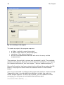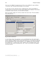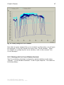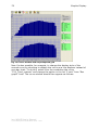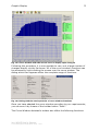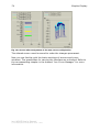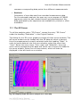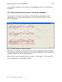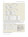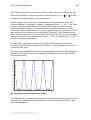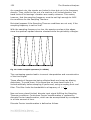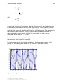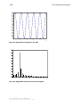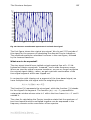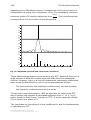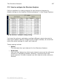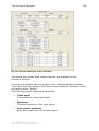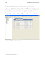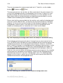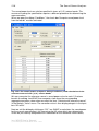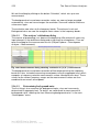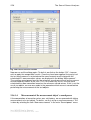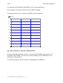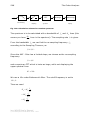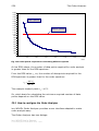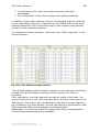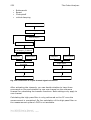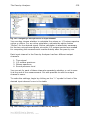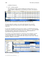
1
imc Meßsysteme GmbH imc WAVE Workstation for Acoustic and Vibration Engineering User's Manual Configuration Software 2 imc WAVE User's Manual © imc Meßsysteme GmbH Berlin 2002 - 2007 Preliminary Remarks Preliminary Remarks 3 Table of Contents Date: Version: 30.03.2007 1.7R1 1 Preliminary Remarks .............................................................. 11 2 Introduction ........................................................................... 23 2.1 2.2 2.3 2.4 2.5 2.6 2.7 2.8 2.9 2.10 3 The Project............................................................................. 27 3.1 3.2 3.3 3.4 3.5 4 Introduction ...........................................................................................43 How to make input channel settings ..........................................................43 Setups .................................................................................... 47 5.1 5.2 6 Introduction ...........................................................................................35 How to create a project............................................................................36 How to open a project .............................................................................39 How to enter the project properties ...........................................................40 What is a project template? ......................................................................41 Input Channels....................................................................... 43 4.1 4.2 5 Data capture ..........................................................................................24 Online data-processing ............................................................................24 Offline data-processing ............................................................................24 Curve display..........................................................................................24 Analysis .................................................................................................24 Import/Export interface ...........................................................................24 Clipboard ...............................................................................................24 Sensor database .....................................................................................25 Calibrator database .................................................................................25 Measurement objects...............................................................................25 Introduction ...........................................................................................47 How to change setups..............................................................................49 Triggers.................................................................................. 52 6.1 6.2 Introduction ...........................................................................................52 How to make trigger settings....................................................................52 7 Analyzers (introduction) ........................................................ 54 8 Graphic Display ...................................................................... 56 8.1 The Screen .............................................................................................56 8.2 How to create a screen ............................................................................56 8.2.1 Creating and modifying screens directly ..............................................57 8.2.2 Working with the Screen Assistant ......................................................59 8.3 Curve windows .......................................................................................63 8.4 How to create a new curve window............................................................64 8.4.1 Directly creating and modifying curve windows ....................................64 8.4.2 Working with the Curve Window Assistant ...........................................66 8.5 How to import screens and curve windows .................................................71 8.6 Using screens and curve windows in concert...............................................72 9 Measurement Data ................................................................. 74 9.1 How to display on-line data from the measurement device ...........................74 9.1.1 How to save on-line measurement data...............................................74 9.2 How to display stored measurement data ...................................................75 9.3 How measurement data are administered ..................................................76 9.3.1 Data overview display .......................................................................76 9.3.2 How to delete data ...........................................................................77 imc WAVE User's Manual © imc Meßsysteme GmbH Berlin 2002 - 2007 4 Preliminary Remarks 9.3.3 9.3.4 9.3.5 How to copy data to the Clipboard ......................................................77 How to group data ............................................................................77 How to export data in different file formats ..........................................78 10 How to Evaluate Measurements ............................................. 80 10.1 The 3D Cursor ........................................................................................81 10.2 The Data Set View...................................................................................83 10.3 How Automatic Analysis works ..................................................................84 10.3.1 Defining a free sequence ...................................................................86 10.3.2 Defining a section .............................................................................86 10.3.3 Creating a program of FAMOS sequences ............................................88 11 The Clipboard ......................................................................... 90 11.1 How to copy data into the Clipboard ..........................................................90 12 The Report ............................................................................. 94 12.1 12.2 12.3 12.4 How to create new reports .......................................................................94 How to print out reports of particular measurements ...................................98 Can reports be administered in groups? ...................................................100 Can the same reports be used in different projects? ..................................100 13 Measurement objects ........................................................... 102 13.1 13.2 13.3 13.4 13.5 13.6 How How How How How How to to to to to to edit the structure of a Measurement object database ......................103 define Measurement object types .................................................105 define components .....................................................................106 create a new object ....................................................................107 assign a type and components to an object ...................................107 assign Measurement objects to their measurements .......................107 14 How to Use the Sensor Database.......................................... 110 14.1 14.2 How to assign available sensors to input channels .....................................110 How to define a new sensor in the sensor database ...................................112 15 How to Use the Calibrator Database..................................... 118 16 How to Adjust the Entire Measurement Chain ...................... 122 16.1 16.2 Manual adjustment................................................................................122 How to perform adjustment....................................................................124 17 imc WAVE Data Structuring Capabilities............................... 126 17.1 Local structuring elements .....................................................................126 17.1.1 The structuring role of projects ........................................................126 17.1.2 The structuring role of groups ..........................................................126 17.1.3 The structuring role of measurements ...............................................127 17.2 Global structuring elements ....................................................................127 17.2.1 The structuring role of measurement object types ..............................127 17.2.2 The structuring role of components...................................................127 17.2.3 The structuring role of measurement objects .....................................127 17.3 A data structure example .......................................................................128 17.3.1 The example application ..................................................................128 17.3.2 Structuring the application...............................................................129 18 The Structure Analyzer......................................................... 132 18.1 18.2 18.3 18.4 18.5 The background of FFT...........................................................................132 How to configure the Structure Analyzer ..................................................140 How to design your own window functions................................................145 Structure-Analyzer and trigger settings....................................................148 Application example: Modal Analysis........................................................152 19 The Sound Power Analyzer................................................... 164 imc WAVE User's Manual © imc Meßsysteme GmbH Berlin 2002 - 2007 Preliminary Remarks 5 19.1 What is sound power?............................................................................164 19.2 How to configure the sound power analyzer..............................................170 19.3 The contribution of environmental corrections...........................................174 19.4 How to perform a measurement with the Sound Power Analyzer .................176 19.5 Extra options ........................................................................................179 19.5.1 Changing the number of measurement points ....................................179 19.5.2 How to change the display of the measurement points ........................180 19.5.3 Subsequent changing of measurement point arrangements .................181 20 The Order Analyzer .............................................................. 184 20.1 20.2 20.3 20.4 20.5 20.6 How order analysis is performed .............................................................184 The mathematical theory behind order analysis ........................................190 How to configure the Order Analyzer .......................................................195 What are virtual channels in the Order Tracking Analyzer? .........................199 What optional parameters exist? .............................................................201 How to perform a measurement with the Order Analyzer ...........................207 21 The Personal Analyzer.......................................................... 208 21.1 21.2 21.3 21.4 21.5 Introduction .........................................................................................208 How to create new output channels .........................................................208 How to create a new FAMOS Sequence ....................................................210 Optional Personal Analyzer settings .........................................................211 The Personal Analyzer working with automated evaluation .........................212 22 The Pass-by Analyzer ........................................................... 218 22.1 What is a pass-by test?..........................................................................218 22.2 How to configure the standard microphone channels .................................218 22.3 Optional parameters in pass-by analysis ..................................................222 22.3.1 Measurement setups and triggers .....................................................222 22.3.2 Options .........................................................................................223 22.4 How to configure additional channels .......................................................226 22.5 How to carry out a measurement ............................................................227 23 The Spectrum Analyzer ........................................................ 230 23.1 What calculated quantities are available? .................................................230 23.2 How to configure the Spectrum Analyzer ..................................................230 23.3 Optional parameters for the Spectrum Analyzer ........................................233 23.3.1 FFT parameter settings ...................................................................234 23.4 How to carry out a measurement with the Spectrum Analyzer ....................235 24 Work Station Noise Analyzer ................................................ 236 24.1 What calculated quantities are available? .................................................236 24.2 How to configure the Workplace Noise Analyzer ........................................236 24.3 Optional parameters for the Workplace Noise Analyzer ..............................238 24.3.1 Frequencies ...................................................................................239 24.3.2 Weighting ......................................................................................239 24.4 Running a measurement with the Workplace Noise Analyzer.......................239 25 Index of illustrations............................................................ 242 imc WAVE User's Manual © imc Meßsysteme GmbH Berlin 2002 - 2007 6 Preliminary Remarks imc Customer Service - Hotline If you have problems or questions, the Hotline can provide help: AUSTRALIA MSC.Software Australia - Melbourne Level 7 271 William Street Melbourne, VIC 3000 Tel.-No.: +61 3 9691 8555 Fax-No.: +61 3 9691 8599 E-Mail: [email protected] AUSTRIA ADDITIVE Hard- und Software für Technik und Wirtschaft GmbH & Co. KG Willergasse 33 1230 Wien Tel.-No.: + 43 1 9828 529-0 Fax-No.: +43 1 9828 52920 E-Mail: [email protected] BELGIUM imc Meßsysteme GmbH Voltastr. 5 13355 Berlin (Germany) Tel.-No.: +49 030 46 70 90 0 Fax-No.: +49 030 46 31 57 6 E-Mail.: [email protected] CHINA Integrated Measurement & Control CO. No. 1802 Room, Gouhengjiye Building E No.7 West Road of Beitucheng Chaoyang District 100029 Beijing Tel.-No.: + 86 10 82275791 Fax-No.: + 86 10 82275791 E-Mail: [email protected] CZECH REPUBLIC Ing. Igor Luhan, CSc., PMP INTEGRACE MĚŘICÍCH SYSTÉMU Práčská 53 106 00 Praha 10 Tel.-No.: + 420 2 72129247 Fax-No.: + 1 561 5948397 E-Mail: [email protected] imc WAVE User's Manual © imc Meßsysteme GmbH Berlin 2002 - 2007 Preliminary Remarks FINLAND UG Electronics Oy Ruukintie 3 02320 Espoo Tel.-Nr.: +358 9 81946622 Fax-Nr.: +358 9 8026699 E-Mail: [email protected] FRANCE JOHNE + REILHOFER France SA 71 Bd de Brandebourg 94854 IVRY SUR SEINE CEDEX Tel.-No.: +33 1 49 59 01 90 Fax-No.: +33 01 46 70 47 30 E-Mail: [email protected] INDIA PT Instruments Pvt. Ltd. 6/6/10, Bhawani Nagar PO Box No. 17436 Marol Maroshi Road, Andehri (E) Mumbai 400 059 Tel.-No.: +91 22 2851 1353 Fax-No.: +91 22 2850 1886 E-Mail: [email protected] ITALY Instrumentation Devices SLR Via Acquanera 34/M 22100 Como Tel.-No.: +39 031 525391 Fax-No.: +39 031 507984 E-Mail: [email protected] JAPAN TOYO Corporation 1-6 Yaesu 1 chome Chuo-Ku Tokio 103-8284 Tel.-No.: +81 3 3279-0771 Fax-No.: +81 3 5205 2030 E-Mail: [email protected] imc WAVE User's Manual © imc Meßsysteme GmbH Berlin 2002 - 2007 7 8 KOREA SV Corporation Room 302 Sangshin B/D, 719-1 Yi-dong, Sangrok-gu Ansan Kyongki-do 426-857 Ansan Tel.-No.: +82 31 501 4030 Fax-No.: +82 31 501 4032 E-Mail.: [email protected] MALAYSIA Info-trax Sdn Bhd 42-3, Jalan Sulaiman 1, Taman Putra Sulaiman 43200 Ampang, Selangor Tel.-No.: + 603 4270 6085 Fax-No.: + 603 4270 6054 E-Mail.: [email protected] NETHERLANDS imc Meßsysteme GmbH Voltastr. 5 13355 Berlin (Germany) Tel.-No.: +49 030 46 70 90 0 Fax-No.: +49 030 46 31 57 6 E-Mail.: [email protected] PORTUGAL ALAVA INGENIEROS, S.A. Dpto. Instrumentación C/ Estebanez Calderón 5 C.P. 28020 Madrid (Spain) Tel.-No.: +34 91 567 9700 Fax-No.: +34 91 570 2661 E-Mail: [email protected] SLOVAKIA Ing. Igor Luhan, CSc., PMP INTEGRACE MĚŘICÍCH SYSTÉMU Práčská 53 106 00 Praha 10 (Czech Republic) Tel.-No.: + 420 2 72129247 Fax-No.: + 1 561 5948397 E-Mail: [email protected] imc WAVE User's Manual © imc Meßsysteme GmbH Berlin 2002 - 2007 Preliminary Remarks Preliminary Remarks SPAIN ALAVA INGENIEROS, S.A. Dpto. Instrumentación C/ Estebanez Calderón 5 C.P. 28020 Madrid Tel.-No.: +34 91 567 9700 Fax-No.: +34 91 570 2661 E-Mail: [email protected] SWEDEN CE-BIT Elektronik AB Polygonvägen 29 187 66 Täby Tel.-No.: + 46 8 735 7550 FAX-No.: + 46 70 493 2006 E-Mail: [email protected] SWITZERLAND imcAdd AG Stammeraustr. 8 Postfach 463 8501 Frauenfeld Tel.-No.: +41 52 7221455 Fax-No.: +41 52 7221459 E-Mail: [email protected] TAIWAN System Access Company Ltd. 6F-4., No. 160, Minchuan East Road, Sec. 6 Taipei R.O.C. 146 Tel.-No.: +886-2-8792-6266 Fax-No.: +886-2-8792-6265 E-Mail: [email protected] UK Metrum Information Storage Limited 2 Weller Drive, Finchampstead Wokingham Berkshire RG40 4QZ Tel.-No.: + 44 118 973 3000 Fax-No.: + 44 118 973 4363 E-Mail: [email protected] imc WAVE User's Manual © imc Meßsysteme GmbH Berlin 2002 - 2007 9 10 Preliminary Remarks USA imc DataWorks, LLC 2923 Market Drive, Suite 102 Madison, WI 53719 Tel.-No.: + 1 608 231 6123 FAX.-No.: +1 608 231 6125 E-Mail: [email protected] You can help us to provide useful hotline service by knowing your version number and keeping this manual handy when calling. This service is only provided for registered customers who purchased their product directly from imc or one of the above listed distributors. imc WAVE User's Manual © imc Meßsysteme GmbH Berlin 2002 - 2007 Preliminary Remarks 11 1 Preliminary Remarks imc (integrated measurement & control) reserves the right to change any of the contents of this documentation without warning. The contents do not represent any obligations on the part of imc. The software described in this document is provided under the conditions stated in the License Agreement. The software may be used or copied only in accordance with the conditions in this agreement. Copying the software to a different medium is permitted only in the cases explicitly allowed in the License Agreement. These manuals may not be reproduced electronically or manually, complete or in part, and may not be duplicated in any way or by any means, e.g. by photocopying or recording unless express written permission has been obtained from imc Meßsysteme GmbH, Berlin. (C) Copyright 2002 imc Meßsysteme GmbH. All rights reserved. Microsoft, MS and MS-DOS are registered trademarks of Microsoft Inc., USA Windows and Windows NT are trademarks of Microsoft, Inc., USA Quality management imc possesses DIN-EN-ISO-9001 certification since May, 1995. In May, 1998, the accredited TÜV CERT certification laboratory of TÜV Anlagentechnik GmbH awarded us a certificate attesting to our conformity to the world-wide accepted standard DIN EN 9001. The Certificate Registration Number is 0910085152. imc WAVE and Microsoft® Windows™ imc WAVE works in a graphical environment called Microsoft Windows which is produced by Microsoft Corporation. Microsoft Windows provides a standardized user interface for imc-Devices software and all other Windows-applications. The imc-Devices product package includes the software needed to operate imc WAVE. Microsoft-Windows offers the following advantages: Running multiple applications: Multiple applications can be run under Windows at the same time, and the user can easily switch from one to the other. This provides an integrated working environment. imc WAVE User's Manual © imc Meßsysteme GmbH Berlin 2002 - 2007 12 Preliminary Remarks Data transfer between applications: Data can be exchanged between imc WAVE and other Windowsapplications. Windows-control of DOS environment: From the Windows-environment, you have easy access to all Windows and DOS applications, files, folders and drives. All MS-DOS functions (such as file management and diskette formatting) can be controlled from Windows. To run imc WAVE under Microsoft Windows, a license for Microsoft Windows 95 or Windows NT 4.0 (or higher) is needed. Microsoft, MS and MS-DOS are registered trademarks and Windows is a trademark of Microsoft Corporation. Intel and Pentium are registered trademarks of Intel Corporation, USA. © imc Meßsysteme GmbH 2002 – 2007 imc WAVE User's Manual © imc Meßsysteme GmbH Berlin 2002 - 2007 Preliminary Remarks 13 imc Warranty and Software-License Agreement1 imc Limited Warranty This is a valid agreement between the user and imc Mess-Systeme GmbH (integrated measurement & control) in Berlin2. This warranty gives you specific rights which may vary from country to country. • imc warrants to the original licensee that the hardware products will be free from defects in material and workmanship for a period of one year after purchase. • imc warrants to the original licensee that the software will properly execute its program instructions when properly installed. • imc warrants to the original licensee that the media on which the program is recorded will be free from defects in material and workmanship under normal use. • imc will replace or repair any hardware faulty components as deemed appropriate. imc is only liable for the replacement of hardlocks or software media after having received them back from the licensee. • If imc is not able to repair or replace a product deemed faulty within a reasonable length of time, the licensee can either request a discount on the original price or receive a full refund of the purchase price. Conditions of Invalidation This warranty does not apply to faults in imc products resulting from: • Inappropriate or insufficient maintenance on the part of the customer. • Software, connective cables and devices, PC's or any other non-imc products supplied by the customer. • Unauthorized changes or inappropriate use. • Operation of the device in environmental conditions exceeding those specified in this user's manual. • Insufficient preparation and/ or maintenance of the operating location. • Disregard of the advice made in this manual concerning installation, operation, transport, maintenance, error handling, etc.. The warranty period begins on the day of delivery or, if the purchase price includes installation, on the day of installation. 1 The data and information contained in these documents may be changed without prior notice. imc may hold rights to patents, trademarks, copyrights and other intellectual property, to which the statements in this documentation refer. This does not imply that the purchaser of this imc product receives any of these rights, excepting such which are explicitly provided for in the written license agreement. 2 The data and information contained in these documents may be changed without prior notice. imc WAVE User's Manual © imc Meßsysteme GmbH Berlin 2002 - 2007 14 Preliminary Remarks Restrictions The above warranty is the only one provided. No other guarantees, whether written or spoken, expressed or implied, are accepted. In particular, imc refuses to guarantee that their products are of typical quality and therefore suitable for any purposes other than those expressly described. In some countries, a restriction of the implied guarantee is not allowed meaning that the above clause is invalid. In any case, a guarantee stating that imc products are of typical quality and therefore suitable for any purposes other than those expressly described, is limited to a maximum one year duration. Liability Restrictions In no event shall imc or distributors of imc products be held liable for incidental or consequential damages, including but not limited to loss of use, loss of revenues or profit, loss of data or data being rendered inaccurate, or losses sustained by third parties even if imc has been advised of the possibilities of such damage. Maintenance Within Warranty Period If hardware failure occurs within the warranty period, please contact imc Customer Support. Please be sure to package your device properly (as specified below) before shipping it back to imc or to your imc distributor. You should always keep the original packaging! The customer is liable for any shipping damage resulting from inappropriate packaging of the product. Wherever possible, reuse the original packaging! Attention Damage during shipping which is caused by inappropriate packing is charged to the customer. Use the original packaging material, therefore, whenever possible. Customer Service After Warranty Expiration If a hardware failure occurs after the warranty period has expired and you have made a special agreement with imc, you only receive service as specified in the special agreement. If you have not made a special agreement of any type with imc, please contact our Customer Support or the distributor concerning servicing of imc products. Return Product Packaging Always try to use the original imc packaging when returning an imc product. Always contact the imc customer service before sending your product to guarantee the most efficient service possible. Be sure to add a brief description of the error or problem and information concerning the configuration and initialization files and any saved experiments. Remarks If you no longer possess the customized packaging material for your imc product, appropriate material can be ordered from imc. imc WAVE User's Manual © imc Meßsysteme GmbH Berlin 2002 - 2007 Preliminary Remarks 15 imc Software License Agreement Important Note Special contract stipulation Before opening the enclosed disk package, please read carefully all of the following conditions. They govern the use of the enclosed software products and documentation for the operation of the system. By opening this sealed disk package, you are agreeing to be bound by the terms of this agreement. Below are the contractual conditions for your, the purchaser's ("the licensee"), use of imc products. Please read carefully the following text in its entirety. Conditions of Agreement 1. Objects of Agreement The objects of this agreement are the computer program saved on the data storage medium (diskettes) and its documentation. In the following, the computer program is referred to as the "software". imc makes no claim that the software runs error-free in all applications and with all platforms. The imc software is thus only to be considered the object of this agreement when used in the manner specified by the documentation. 2. Grant of License imc grants you, for the duration of this agreement, the single right to use the enclosed copy of the imc software on a single computer (i.e., on a single CPU) and to be used only at one site. If this single computer is a multi-user network, the user rights are valid for all users of this network. You may make copies of the program solely for backup purposes, provided you reproduce and include the copyright notice on any backup copy. As licensee, you are allowed to physically transfer the software (saved on a diskette) from one computer to another computer, under the stipulation it only be used on one computer at any moment. Software is "in use" on a computer when it is loaded into temporary memory (i.e. RAM) or installed into permanent memory on a computer (i.e. hard disk, CD-ROM, etc.). Any more extended use is not permitted by this agreement. 3. Special Restrictions The licensee is forbidden, a) to distribute copies of the software and/or documentation to third parties; b) to provide use of the program through a computer service business, network or other data transfer channel; c) to translate, reverse-engineer or alter the software and its documentation; d) to rent, lease, or grant sublicenses or other rights to the program; without the prior written consent of imc. imc WAVE User's Manual © imc Meßsysteme GmbH Berlin 2002 - 2007 16 Preliminary Remarks 4. Rights of Possession The purchase of this product only entitles you, the licensee, to ownership to physical data carrier where the software is saved. You do not acquire any rights to the software and documentation. imc reserves all publishing, copying, processing and management rights for the software and documentation. 5. Copyright imc owns this software program and its documentation. Both the program and documentation are copyrighted with all rights reserved by imc. For software not equipped with copy protection, you may make one single copy of the program solely for backup purposes, provided you reproduce and include the imc copyright notice on the backup copy. The copyright incorporated in the software is not to be removed or altered in any way. It is strictly forbidden to copy or reproduce the software and documentation: a) entirely or partially, b) in its original form, c) in an altered form, d) in combination with other software or, e) contained in other software. This software product is licensed to you as a unit. You are not entitled to separate it into components with the intent to use these simultaneously in different computers. 6. Transfer Of User Rights The software license may only be transferred to a third party with the prior written consent of imc and only under the conditions of this contract. It is explicitly forbidden to rent, lease, or grant sublicenses or other rights to the program without the prior written consent of imc. 7. Duration of License Agreement The duration of the contract is indefinite. Your license to use the program and documentation will automatically terminate if you fail to comply with the terms of this Agreement. If this license is terminated, you agree to destroy all copies of the program and documentation, or any altered versions thereof, in your possession. 8. Compensation In Case of License Termination imc draws attention to the fact that you will be held liable for any damage which may ensue following termination of this license agreement. 9. Software Updates and Improvements imc reserves the right to update and improve the software as deemed appropriate. imc WAVE User's Manual © imc Meßsysteme GmbH Berlin 2002 - 2007 Preliminary Remarks 17 10. Guarantee And Liability Of imc a) imc warrants to the original licensee that the hardware components are errorfree under normal operating conditions at the time of delivery. b) If the data carriers (disks) or the supplied hardware (e.g. hardlock) are faulty, the licensee can request a replacement within the 12 month guarantee, from delivery. The disks supplied with the delivered material and a copy of the invoice must be returned to imc or to the distributor. c) If a fault as described in 10 b) above is not repaired, removed or eliminated by a replacement delivery within a reasonable length of time, the licensee can either request a discount on the original price or have the contract declared null and void. d) Based on the stipulations stated in 1 above, imc will not be held liable for errors in the software. imc especially gives no guarantee that the software is suitable for the requirements and objectives of the licensee or that the software is compatible with other programs used by the licensee. The licensee is responsible for the purchase of the software and its compatibility with its intended platform. If the software is not useable in the sense of 1 above, the licensee has the right to negate the contract. imc maintains the same right if development of appropriate software is not possible with reasonable effort. e) In no event shall imc be liable for incidental or consequential damages, including but not limited to loss of use, loss of revenues or profit, loss of data or data being rendered inaccurate, or losses sustained by third parties even if imc has been advised of the possibilities of such damage. Sales representatives or distributors will not be held liable or negligent for any damage or losses. Liability on the part of imc for failing to meet specified ratings or properties is not affected by these terms. 11. Jurisdiction This license agreement shall be governed by the laws of Germany with jurisdiction in Berlin. imc WAVE User's Manual © imc Meßsysteme GmbH Berlin 2002 - 2007 18 Preliminary Remarks Product improvement Dear Reader! We at imc hope that you find this manual helpful and easy to use. To help us in further improving this documentation, we would appreciate hearing any comments or suggestions you may have. In • • • • particular, feel free to give us feedback regarding the following: Terminology or concepts which are poorly explained Concepts which should be explained in more depth Grammar or spelling errors Printing errors Please send your comments to the following address: imc Meßsysteme GmbH Customer Support Voltastraße 5 D - 13355 Berlin Telephone: +49 - 30 - 46 70 90 - 26 Fax: +49 - 30 – 463 15 76 e-mail: [email protected] imc WAVE User's Manual © imc Meßsysteme GmbH Berlin 2002 - 2007 Preliminary Remarks 19 Although graphically oriented programs such as imc WAVE are designed to be used intuitively, we recommend reading through the user’s manual. You'll discover interesting functions, many of which you may previously not have been aware of. The technical specifications stated in these chapters are valid for 1 year from the device's delivery date and for use under normal operating conditions. Note in particular the ambient temperatures specified. Symbols displayed on the equipment ! CAUTION! REFER TO THE USER'S MANUAL. This symbol advises the user to consult the User’s Manual for more information concerning possible dangers. DANGER: HIGH VOLTAGE1 This symbol is used anywhere on the device where a high-voltage danger exists. Only trained maintenance personnel may perform repairs to any of these areas. DANGER OF ELECTROSTATIC DISCHARGE Electrostatic sensitive devices, that is any electronic components at risk of damage due to electrostatic discharge (ESD), are denoted by this symbol. imc WAVE User's Manual © imc Meßsysteme GmbH Berlin 2002 - 2007 20 ESD WARNING! Despite protective measures, our components are sensitive to electrostatic discharge. Electrostatic charge may build up unnoticed and may even cause damage without your being immediately aware of it. Such damage can be avoided by carrying out all work at "safe" work stations and by utilizing packaging with electrostatic shielding when transporting sensitive components. Always follow ESD precautions! ATTENTION! • When handling static-sensitive devices, observe the following guidelines: • Always statically discharge yourself (e.g. by touching a grounded object) before handling static-sensitive devices. • Any equipment and tools used must also be free from static charge. • Unplug the power cord before removing or inserting static-sensitive devices. • Handle static-sensitive devices by their edges. • Never touch a connection pin or conducting track on static-sensitive devices. Always ensure that electrostatic charge does not form at contacts between device sockets and their leads. Any charge which may develop here is to be drained off. Damage resulting from ESD is not covered in the guarantee. imc WAVE User's Manual © imc Meßsysteme GmbH Berlin 2002 - 2007 21 Hardware Requirements Minimum required hardware configuration: IBM - (100%-compatible) AT with Pentium processor hard drive with min. 100 MByte free memory plus memory requirements of MS Windows DC-ROM drive (for installation) graphics card supported by MS - Windows with 800x600 pixels and matching monitor AT-keyboard 32 MByte RAM mouse (bus or serial) supported by MS - Windows, Microsoft-mouse or compatible mouse, Logimouse (many MS-Windows functions work easier and faster through the use of a mouse) We recommend: upgrade to 128 MByte RAM or more processor: Pentium 3 –500 (or compatible) or higher, to guarantee rapid display of high data volume graphics card with 1024 x 768 pixels at 65000 colors and a refresh rate from 70 Hz on Additional options MS - Windows supported printer (almost all printers) Software requirements and restrictions The following prerequisites are required to run imc WAVE: 32-Bit Windows (Windows 2000, Windows XP) We do not guarantee that the software will run under any future version of these operating systems. Memory management It is well known Microsoft Windows allows "multitasking", that is, several programs can be loaded to memory and run at once. In actual fact, however, the computer can only run any one application at a given moment. But, as far as the user is concerned, several applications are available and can be run virtually in parallel. The imc WAVE software is designed with true multitasking in mind, that is, its program code has been divided into many smaller segments. However, imc WAVE also uses RAM to store its waveform data, and when a lot of data are present, this can consume all of the available memory. It is thus not recommended to run many programs at once. imc WAVE retains data in RAM as long as there is sufficient space there. Otherwise imc WAVE stores its data on the available drives (disks). The default folder is the environmental variable "Temp" or "Tmp" under Windows. imc WAVE User's Manual © imc Meßsysteme GmbH Berlin 2002 - 2007 22 imc WAVE User's Manual © imc Meßsysteme GmbH Berlin 2002 - 2007 Introduction 23 2 Introduction The imc Workstation for Acoustic and Vibration Engineering (referred to below as imc WAVE) is an application adapted to the requirements of sound and vibration measurement engineering. Different analyzing tools are dedicated to each of the areas of this field, for instance: - FFT-Analyzer Sound power Order analysis Fig. 1: imc WAVE user interface imc WAVE is project-oriented and provides the user with a simple operating interface. A project is begun by selecting an analyzer. This analyzer presents a window as a table offering settings. There are additional windows used by all the analyzers in common, such as trigger settings, connection configuration, curve window etc. To navigate within a project, the Project Explorer can be used, which enables all functions to be accessed after only a few clicks. To organize the various actions possible, the functions are arranged in function groups. The Project Explorer orders the available actions according to their necessary sequence and thus conforms to imc's guiding design principle: imc WAVE User's Manual © imc Meßsysteme GmbH Berlin 2002 - 2007 24 Introduction ...all the way from the sensor to the data sheet printout... Below is a short introduction to the subgroups, which are explained in detail in later chapters. 2.1 Data capture Data capture is performed by a hardware system comprising up to 16 input channels each operating at 50 kHz. The user interface provides control of the system. 2.2 Online data-processing The result data are computed whenever possible during a running measurement. 2.3 Offline data-processing For processing data coming from other sources, off-line analysis can be performed. The calculations done are based on the settings for the data acquisition. Thus, data already captured can be re-processed by changing the settings. 2.4 Curve display There are screen windows for display of data. A screen can comprise up to four such curve windows. As a rule, all imc curve window settings can be made using the right mouse button. For ease of operation, the most important functions are also available via the menu and the toolbar in the main window. 2.5 Analysis Data analysis is already under way during data capture. For printout, standard templates are available which can be easily filled and printed out by point-&-click. It is also possible to create layouts and to incorporate these into an existing project. In addition, a variety of graphic analysis techniques is available, from comparisons all the way to 3D waterfall and color map representation. 2.6 Import/Export interface The import/export interface offers a variety of data types for importing and exporting measurement data. The data to be saved are selected and written to the drive in the desired format. 2.7 Clipboard The Clipboard makes it possible to keep data constantly at hand within a project, no matter what measurement is currently selected. This means imc WAVE User's Manual © imc Meßsysteme GmbH Berlin 2002 - 2007 Introduction 25 that reference or tolerance curves can be added to and displayed in a curve window. The data can either be placed into the Clipboard directly from a measurement, or you can use imc FAMOS to generate a data set and load it to the Clipboard. 2.8 Sensor database For quick parameterization of the inputs, a database for sensor data is provided. This database can be extended as desired by the user. 2.9 Calibrator database The calibrator database is the logical extension of the sensor database. A calibrator for the calibrator database can be assigned to each sensor from the sensor database. This calibrator is used as the basis for adjusting the sensor. This makes it unnecessary to specify the calibrator's vibration values prior to the adjustment process. 2.10 Measurement objects Measurements are performed on measurement objects. The measurement objects can be entered in a database and assigned to the appropriate measurements for better clarity. This makes it possible to compare only the measurements of a particular measurement object or to view the particular measurement object for a pool of measurements. The measurement objects are organized hierarchically and consist of measurement object types and measurement object components. imc WAVE User's Manual © imc Meßsysteme GmbH Berlin 2002 - 2007 26 imc WAVE User's Manual © imc Meßsysteme GmbH Berlin 2002 - 2007 Introduction Installing imc WAVE 27 3 Installing imc WAVE This chapter provides instructions for installing imc WAVE, as well as tips concerning and answers to common questions related to the installation of imc WAVE. 3.1 imc WAVE installation instructions Before installing imc WAVE, all other applications, especially imc programs, should be closed. If you already have a version of imcDevices or imc WAVE on your PC, first uninstall these programs. Place the installation-CD in the drive and start the program “SETUP.EXE“. Select the language in which to carry out the setup program. Fig. 2: Selecting the installation program language Next, you can decide whether you wish to install imc WAVE, whether to read the documentation on the CD, and whether to install an Acrobat Reader for the purpose of reading the documentation. imc WAVE User's Manual © imc Meßsysteme GmbH Berlin 2002 - 2007 28 Installing imc WAVE Fig. 3: Selection dialog for the installation Here, select “Install Software”. In the subsequent dialog you are prompted for the installed software’s language. Select the language which you prefer for imc WAVE as well as imcDevices. Fig. 4: Selection of the language version for the installed software imc WAVE Once you have selected the language and have clicked on the OK button, the actual installation program for imc WAVE is started. imc WAVE User's Manual © imc Meßsysteme GmbH Berlin 2002 - 2007 Installing imc WAVE 29 Fig. 5: Welcome dialog of the imc WAVE installation program If you now click on “Next”, the system checks whether any version of imc WAVE or imcDevices is already installed on your PC. A message such as the one shown below may appear: Fig. 6: Notification of an installed version of imcDevices If such a notification appears, stop the installation program and uninstall the version of imcDevices. The uninstalling procedure can be carried out by selecting the Control Panel item “Add/Remove Programs”. From the list of programs which then appears, select the entry for imcDevices or imc WAVE and click on the Change or the Remove button. imc WAVE User's Manual © imc Meßsysteme GmbH Berlin 2002 - 2007 30 Installing imc WAVE Fig. 7: Uninstalling imcDevices If no notification appears, the installation program starts automatically and installs imc WAVE and the associated version of imcDevices on your PC. In the next dialog, you can select the installation folder for imc WAVE. Fig. 8: Selecting the installation folder for imc WAVE You will be prompted to choose the group in the Start menu in which to create a shortcut to imc WAVE. It is also possible to create a new group for the purpose. imc WAVE User's Manual © imc Meßsysteme GmbH Berlin 2002 - 2007 Installing imc WAVE 31 Fig. 9: Selecting the optional parameters and the directory of imcDevices You can choose the optional parameters and the installation directory of imcDevices in the following dialog. The assistant for the CAN Bus interface will be installed automatically. Further options can be installed by selecting the corresponding lines in the list. For some of the options password are necessary. You got the passwords with the delivery of your system, if you have ordered the option. Fig. 10: Selecting a group in the Start menu imc WAVE User's Manual © imc Meßsysteme GmbH Berlin 2002 - 2007 32 Installing imc WAVE With this, the preparations for the installation are completed and the actual installation process can begin. You can move through the sequence of dialogs by using the buttons “Back” and “Next”. Fig. 11: Completing preparations for installation Once the button “Next” in the last dialog has been clicked, installation of imc WAVE begins. Along with imc WAVE, a version of imcDevices is also installed, namely to the default folder C:\imc\imc devices. Once all components were installed, the following dialog finally appears: imc WAVE User's Manual © imc Meßsysteme GmbH Berlin 2002 - 2007 Installing imc WAVE 33 Fig. 12: Completing installation Now imc WAVE and imcDevices are installed on your hard drive. To start one of the programs, click on the corresponding shortcut. If you are working with imc WAVE for the first time, observe the notes in the imc WAVE instructions manual as well as the notes in the manual for imcDevices or your measurement system. If you have any questions or need tips, the authorized distributor for your area will be happy to help you. If you discover any mistakes or have comments on this installation or on the manual, please contact us directly at [email protected] . 3.2 Frequently asked questions 3.2.1 Can I use a different version of imcDevices with imc WAVE? As a matter of principle, your version of imc WAVE has been tested with one version of imcDevices. If you use a different version, then it could happen that incompatibility will cause imc WAVE to not work correctly. For instance, if an older version of imcDevices is used, imc WAVE could try to access imcDevices functions which weren’t available until the present version. When in doubt, your local authorized distributor will be happy to assist you. 3.2.2 How can I install a new version of imcDevices? imc WAVE accesses the imcDevices functions via the COM objects. Upon installation of imc WAVE, a RUNTIME version of these COM objects is imc WAVE User's Manual © imc Meßsysteme GmbH Berlin 2002 - 2007 34 Installing imc WAVE installed on your PC. When imcDevices is uninstalled, these RUNTIME objects are uninstalled along with it, since they wouldn’t be compatible with any newly installed version. If you install a new version of imcDevices, it is necessary to install the imcDevices COM objects along with it. However, before you can install them, you will need a working installation of the basis COM objects from imc. These basis COM objects must be installed prior to installation of imcDevices. They aren’t included in either imcDevices or imc WAVE and must be purchased separately. To learn more, your local authorized distributor will be happy to assist you. imc WAVE User's Manual © imc Meßsysteme GmbH Berlin 2002 - 2007 The Project 35 4 The Project imc WAVE is a project-oriented program package which administers and displays all data together with the project to which they belong. 4.1 Introduction A project has the following components • • • • settings data displays and output options. This somewhat abstract characterization may become clearer by taking a look at imc WAVE's Project Explorer. Fig. 13: imc WAVE Project Explorer The Project Explorer is the easiest way to navigate through a project. In the Project Explorer you get a clear picture of a project's structure. imc WAVE User's Manual © imc Meßsysteme GmbH Berlin 2002 - 2007 36 The Project A project consists of: • • • • • • • • the the the the the the the the configuration of the input channels configuration of the triggers analyzer settings displays analysis options data Clipboard reports. The individual items are described below. Each of the items presented by the Project Explorer pertains to a particular project. When you switch to a different project, the data for the new project are opened and displayed in the Project Explorer. It may become desirable to load settings from one project (e.g. the data display options) into another project. This can be accomplished using an import interface. See further below for details. Alongside the settings particular to the projects there are also global settings which apply to all projects. These include, for example, the measurement objects and the sensor database. The data for these settings are administered globally and are available to all projects. imc WAVE's project management system makes a compressed summary of all data and settings which are saved under a common project name. 4.2 How to create a project The first step towards performing a measurement is to create a new project. You are prompted to do this when imc WAVE is started. imc WAVE User's Manual © imc Meßsysteme GmbH Berlin 2002 - 2007 The Project Fig. 14: imc WAVE Start dialog The Start dialog offers you the choice of creating a new project, or opening the last project or any other already created project. When you create a new project, the following dialog appears. imc WAVE User's Manual © imc Meßsysteme GmbH Berlin 2002 - 2007 37 38 The Project Fig. 15: Creating a new project To create a project, the program requires • • • • a folder in which to save the project, a name under which to save the project, selection of the desired analyzer, and of the measurement devices with which to carry out the measurement The analyzers from which to choose are presented in a list. The available selection of analyzers depends on which ones are enabled for your device (for detailed information, see the chapter: “How to enable analyzers”). Once all information has been entered and confirmed by pressing the OKbutton, the project is saved under the selected name in the selected folder. You can now proceed to configure the project and perform measurements. Towards this end, once the definitions dialog is closed, the main imc WAVE window appears. In this main window, you can make all entries necessary for carrying out and administering the project. imc WAVE User's Manual © imc Meßsysteme GmbH Berlin 2002 - 2007 The Project 39 In the project's main menu, the "File" menu contains items for administering the projects. These include: • New project ... Creates a new project with the help of the dialog described above. • Open project ... Loads an exiting project. • Save project as ... Saves the entire active project under a different name. • Delete project ... Totally deletes the project from the hard drive. • Close project ... The project is closed but not deleted. • Project properties ... Displays the project's properties. • Save project as template ... Saves the project as a template and can be selected when creating a project. 4.3 How to open a project If you select the menu item "File – Open project ", the following dialog appears on the screen. Fig. 16: Opening a project This dialog can be used to load a previously created project. The dialog's left side shows a file explorer which you can use to browse through your imc WAVE User's Manual © imc Meßsysteme GmbH Berlin 2002 - 2007 40 The Project computer's filing structure for folders containing projects to select. If you are already in a folder containing projects, these are automatically indicated in the table on the dialog's right-hand side. In this table, each project has its own line. These lines contain additional information, which includes: • Name The project's name • Analyzer Analyzer with which the project was created • Created The project's creation date • Modified The date when the project was last modified These data enable a project to be identified exactly. To load one, click on the desired line in the table to select it, which is indicated by an arrow beside it. When you then close the dialog using the "OK" button, the currently selected project is loaded. If you click on "Cancel", you exit the dialog without loading any new project. 4.4 How to enter the project properties imc WAVE enables you to save information on your project. To do this, double-click on the project's name in the project explorer's top row. imc WAVE User's Manual © imc Meßsysteme GmbH Berlin 2002 - 2007 The Project 41 Fig. 17: Dialog for entering the project properties The dialog for describing the project presents the information provided by imc WAVE, such as • • • • the the the the project's name, project's base directory, project's date created, and date most recently modified, as well as the ability to add more data. For this purpose, the boxes • • • Processed by Project information, and Comment are provided. These data are stored globally in the project and are overwritten upon every change. 4.5 What is a project template? imc WAVE assigns one analyzer to each project. The user supplies these analyzers with specific supplemental data such as display and analysis choices in order to meet the given requirements. Thus, the project represents a complete description of your measurement task. Naturally, it's a pretty big job to collate all the data for a project, especially when dealing with repeated measurement runs which are to be administered in a number of different projects. Thus, imc WAVE comes with the option to save project templates. Such a template would then be an available imc WAVE User's Manual © imc Meßsysteme GmbH Berlin 2002 - 2007 42 The Project choice when creating a project, in which the specific project data you have defined are already provided. You define your project and can already run some measurements in order to check that all settings have been made correctly. Then you can select the project by way of the menu item "File – Save project as template". You are then prompted to enter the template's name. Fig. 18: Name of the project template Enter a name and confirm it by clicking on the OK button. Then the project has been saved as a template. The next time you create a new project and open the dialog for configuring the new project, this project template appears in the list of analyzers. Fig. 19: Creating a new project with the help of a project template Thus, you can consider the project template to be a new analyzer. You thus have the ability to create template analyzers from your own projects, which contain all necessary settings and which can be run at the push of the Start-button. imc WAVE User's Manual © imc Meßsysteme GmbH Berlin 2002 - 2007 Input Channels 43 5 Input Channels 5.1 Introduction imc WAVE distinguishes between the input and output channels of the analyzer selected. The physical inputs of the measurement system you use are referred to as the analyzer's input channels. The number of input channels and their properties depend on your particular device. The analyzer selected processes the measurement device's physical input channels to determine the output channels' signals. Example If you select a Structure Analyzer and have it compute the input channels' auto power density spectrum, the auto power density spectrum amounts to the analyzer's output signal. The formal separation between input and output channels is reflected in the Project Explorer. Configuration of the input channels takes place under the heading "Input channels", configuration of the output channels under the analyzer involved. Settings for the input and output channels are particular properties of a project. If the configuration is changed between individual measurement runs, a new setup is thus automatically created, in which further operation proceeds. Measurements carried out by the present time are still associated with the old setup, so that the configuration is not lost but can be restored. For detailed information on creating and administering setups, consult the chapter of this manual which is devoted to them. 5.2 How to make input channel settings Clicking on the entry "Input channels" in the Project Explorer opens the dialog for configuring the input channels. imc WAVE User's Manual © imc Meßsysteme GmbH Berlin 2002 - 2007 44 Input Channels Fig. 20: Configuring input channels Each channel can be configured separately. The following settings options are available: • Pin Permanent identifier for the input channel • Name Freely specified by the user, however, be sure that the name does not include any special characters if the data are to be subjected to further processing by other programs (e.g. imc FAMOS). • Sensor When this button is pressed, the sensor database's selection dialog appears. You then have the ability to link your input channel permanently to a sensor's output, and thus to load its settings directly from the sensor database. Since some sensors have multiple outputs, (e.g. triaxial sensors or impedance probes) the output you select in the box "output" is displayed in the configuration line. • Output The name of the selected sensor's output, taken from a sensor database, is displayed in this box. If the input channel isn't linked to a sensor database, the box remains empty. Linking the database can be carried out by pushing the button "Sensor". • Reference level Definition of the reference level for converting the physical measurement quantity to a level; if a reference level is specified, imc WAVE User's Manual © imc Meßsysteme GmbH Berlin 2002 - 2007 Input Channels 45 conversion is performed on-line during the measurement. If zero is specified as the reference level, the measurement quantity is returned with a linear y-axis. • Coupling Type of coupling to the measurement device (e.g. AC or DC). The available choices depend on the measurement device used. • Unit The input channel's physical unit. • Gain Scaling factor for converting the raw data to the desired physical quantity; the specification is in the physical measurement quantity/ Volt (e.g. 25.4 Pa / V). • Range End value of the range; the available choices depend on the measurement device used. • Offset Here you can set an offset to add to the physical measurement quantity. Specified in the input signal's physical unit. • Adjustment Information about the last adjustment process of these channel • Input Please choose here the kind of input circuit your sensor needs Once all these parameters have been entered, configuration of the input channel is complete. You also have the possibility to switch from a two-column display to a single-column display. To do this, right-click in the dialog and remove the checkmark in front of the menu entry "Two-line display". The configuration data are then displayed in a line for each channel. If you have linked the channel with a sensor from the sensor database, you can switch off all settings, which are determined by the sensor database. To do this, right-click in the dialog and remove the checkmark in front of the menu entry "Display configuration data". Then, only such configuration data will be displayed which are not determined by the sensor database. The dialog also offers more functions which are accessed by right-clicking the mouse over the button in front of each input channel. imc WAVE User's Manual © imc Meßsysteme GmbH Berlin 2002 - 2007 46 Input Channels This calls a menu offering the following options: • • • • • Sensor database This menu item calls the selection dialog for the sensor database, from which you can select a sensor to link with the current channel. Disconnect If you have already linked a sensor from the sensor database to the current channel, this menu item lets you remove the link while retaining the other channel settings. Sensor definition If a sensor from the sensor database is already linked to the current channel, you can access the sensor settings directly from here. Adjustment This menu item calls the dialog for performing adjustments for the current channel. How to carry out adjustments is described in another chapter. Two line Display Toggle between display of the configuration data in one or two lines. imc WAVE User's Manual © imc Meßsysteme GmbH Berlin 2002 - 2007 Setups 47 6 Setups 6.1 Introduction A setup in imc WAVE refers to the configuration of all components, including the configuration of the input channels, the output channels, the trigger settings etc. An example can serve to illustrate the administration of setups: We create a new project, configure it according to our requirements and carry out approx. 100 measurements. Now, after about 100 measurements, we notice that the wrong windowing function has been set for the FFT. But we don't wish to discard the 100 measurements, since in spite of the incorrect setting we have gained some useful information worth analyzing. We reset the windowing function and start over until we obtain the desired amount of measurements, say 200. Now we have 100 measurements performed using window function X and another 100 using window function Y. After 12 weeks we decide to analyze the data but no longer remember which data were performed using which function. This hypothetical situation will not necessarily reflect your actual experimental practice, of course. There are two approaches to solving the problem outlined above: 1. Make an extensive and accurate lab report at the right time. 2. Perform the whole experiment using imc WAVE. Solution 1 is up to the user. In Solution 2, imc WAVE handles the administration of the entire configuration for you, in the background. imc WAVE notices if the configuration changes during a running measurement and automatically associates the data with a new setup. This means you don't need to take care of the administration and experiment logging yourself, but can instead concentrate on dealing with the substance of your task. When you view data, the correct configuration is automatically indicated, or you can intentionally load a certain setup and conduct the next measurement using it. imc WAVE User's Manual © imc Meßsysteme GmbH Berlin 2002 - 2007 48 Setups Fig. 21: Display of the current setup The setup currently selected is displayed in the Project Explorer after the project name. The default names assigned by imc WAVE for setups are simply serial numbering. Administration of the setup is performed via the menu item "Setups". Here you can activate individual setups manually and edit their names. Under the menu item "Setups – Options", you can determine whether or not the setups for the current measured data are loaded. Fig. 22: Setup options Another example will explain this: imc WAVE User's Manual © imc Meßsysteme GmbH Berlin 2002 - 2007 Setups 49 We have made the 200 measurements described above and now page through the measurements to view them (see also the chapter on displaying measurements). For instance, we view Measurement 98, which was conducted with the 1st setup and next Measurement 102, conducted with the 2nd setup. If the option "Load setting of current measurement data" is activated, the matching setup for the data is automatically loaded. If the option is not activated, the last setup used for a measurement is loaded. Note that if this option is activated and you last view Measurement 98 before proceeding with a new measurement, the new measurement is carried out using Setup 1, even though the most recently performed measurement used Setup 2. Therefore, if this option is active, always make sure of which setup was used with the current measurement. However, it is always possible to manually activate the desired setup and the configuration of your measurement system is totally adaptable. 6.2 How to change setups imc WAVE offers the following possibilities for accessing different setups: • • • Activate Rename … Import These choices are available in the "Setups" menu in the imc WAVE main window. Activating a setup You can activate any setup of your choice, for instance, in order to carry out measurements according to that setup. To do this, select the menu item "Setup – Activate…". Fig. 23: Selection dialog of setups to activate imc WAVE User's Manual © imc Meßsysteme GmbH Berlin 2002 - 2007 50 Setups In the subsequent dialog, all of the project's setups are listed, each with an entry for its name, date created, date last used, and any comment which may have been recorded. The arrow in the table's first column indicates which setup is currently selected. Simply by re-positioning this arrow, you can select a different setup. Changing a setup's name Setups are assigned a default name, so that it's not necessary for you to supply one when creating a new setup. But if you wish to change a setup's name, select the menu item "Setup – Rename". In the dialog which then appears, the setup's name can be edited. Fig. 24: Editing a setup's name Importing a setup You also have the option to import setups from other projects. To do this, select the menu item "Setup – Import". The dialog which then appears presents all setups belonging to known projects of the same type as the project on which you're currently working. Fig. 25: Importing setups from other projects The list may also display some projects shaded gray, which means they are disabled. Such projects are structured differently (e.g. the number of devices involved is different), so that the setup concerned couldn't be imported into your project. imc WAVE User's Manual © imc Meßsysteme GmbH Berlin 2002 - 2007 Setups To import a setup, select the one desired and confirm your choice by clicking on the button "Import". imc WAVE User's Manual © imc Meßsysteme GmbH Berlin 2002 - 2007 51 52 imc WAVE User's Manual © imc Meßsysteme GmbH Berlin 2002 - 2007 Setups Triggers 53 7 Triggers 7.1 Introduction imc WAVE supports one trigger. For each channel, an event, called a trigger event, can be defined, whose occurrence causes an action to take place. The events can be composed of conditions linked by the logic operators "AND" or "OR". You thus have the option to use the signal of any of your analyzer's input channels as the triggering event for the measurement, or to link events. The trigger's configuration is one of a project's properties. Triggered measurement is no longer supported for measurements carried out with multiple devices. If the devices were synchronized before the start of the measurement, however, the order of the data is correct. 7.2 How to make trigger settings The trigger's configuration is displayed when you click on the entry "Trigger" in the Project Explorer. Fig. 26: Configuration dialog for the trigger To define a trigger, activate the desired input channel in the trigger dialog. Next, you select the event type. The various options available for this are selected by making the appropriate settings for the following parameters: imc WAVE User's Manual © imc Meßsysteme GmbH Berlin 2002 - 2007 54 Triggers Threshold value Definition of a threshold value "Threshold 1" with the following events • Positive slope trigger event is rising slope passing through the threshold, • Negative slope trigger event is falling slope passing through the threshold, • Greater than threshold trigger event is measured values higher than threshold, • Less than threshold trigger event is measured values lower than threshold. Range Definition of a signal range with the limits "Threshold 1" and "Threshold 2" • Entering range trigger event is measured values entering range, • Exiting range trigger event is measured values exiting range, • Within range trigger event is measured values falling within range, • Outside range trigger event is measured values falling outside of range, After the events are defined, a pretrigger and event linking can also be set up. The various analyzers each have their own particular settings (e.g. manual takeover for the Structure Analyzer); these settings will be discussed in connection with their respective analyzers. imc WAVE User's Manual © imc Meßsysteme GmbH Berlin 2002 - 2007 Analyzers (introduction) 55 8 Analyzers (introduction) Formally, an analyzer transforms the input signals into output signals by means of an algorithm. The output signals are then available for display and evaluation. An analyzer is selected when creating a project and is permanent for the duration of the project. It is a fixed property of a project; it cannot be changed within a project. Depending on the analyzer selected, different settings and processing steps are available. The description of the analyzers will appear further below. imc WAVE User's Manual © imc Meßsysteme GmbH Berlin 2002 - 2007 56 imc WAVE User's Manual © imc Meßsysteme GmbH Berlin 2002 - 2007 Analyzers (introduction) Graphic Display 57 9 Graphic Display Display of measurement results in imc WAVE is based on the imc curve window. We distinguish between a "screen" and a "curve window", where a screen can comprise multiple curve windows. 9.1 The Screen A screen is a collection of curve windows within a window. There are any number of ways to make and save layouts of graphics displays. A screen is a property of a particular project but can be imported from another project. Already saved screens are to be found in the Project Explorer under the heading "Displays – Screen Assistant". Fig. 27: Screens in the Project Explorer 9.2 How to create a screen There are two ways to create a new screen. 1. Directly, using the main menu This interface provides a relatively quick and easy way to create or modify screens during "running" operation. 2. With the aid of the Screen Assistant The Screen Assistant is an easy-to-use graphical interface specially designed for setting up screens quickly and easily. To use it, however, it's necessary to call the Assistant separately. Both options have their advantages and disadvantages. The two methods are described below. imc WAVE User's Manual © imc Meßsysteme GmbH Berlin 2002 - 2007 58 Graphic Display 9.2.1 Creating and modifying screens directly To create a new screen, start by clicking on the menu item "Screen – New" and in the dialog which then appears enter a name for the new screen. A new entry will then appear in the Project Explorer, having the name you previously entered. The screen name may have a maximum length of 29 characters. The new screen appears in imc WAVE's workspace. Now you can choose how many curve windows to place in the screen. To do this, click on the menu item "Screen – Partition", where the following options are offered: Fig. 28: Single screen Fig. 29: Vertical two-tile screen imc WAVE User's Manual © imc Meßsysteme GmbH Berlin 2002 - 2007 Graphic Display Fig. 30: Horizontal two-tile screen Fig. 31: Vertical three-tile screen Fig. 32: Horizontal three-tile screen imc WAVE User's Manual © imc Meßsysteme GmbH Berlin 2002 - 2007 59 60 Graphic Display Fig. 33: Four-tile screen Depending on the partitioning selected, one to four curve windows are displayed on your screen. The layout of the screens is constant, but the size of the screens can be changed. To do this, you can grab the bar between the curve windows by clicking and holding down the left mouse button over it, then shift it to the desired location and leave it there by releasing the mouse button. Each of these curve windows can be configured individually. Configuration is described in the next section. After adapting the screens (size, partitioning, assignment of curve configurations, etc.) the screen must be saved so that the changes will be restored upon the next call. For this purpose, the menu items "Save" and "Save as.." are available in the "Screen" menu. Additionally, you can edit a screen's name or delete whole screens. For this, there are corresponding menu items. 9.2.2 Working with the Screen Assistant The Screen Assistant is started by double-clicking on the Explorer entry "Screen Assistant" under "Display". imc WAVE User's Manual © imc Meßsysteme GmbH Berlin 2002 - 2007 Graphic Display 61 Fig. 34: Screen Assistant The Screen Assistant consists of a toolbar and its associated screen below. You can use the toolbar tools to either generate screens or to modify existing screens. We now create a new screen by clicking on the icon . We will then be prompted to supply a name for the new screen and enter a name in the dialog which then appears. Fig. 35: Name for the new screen After confirming, the screen looks like the illustration below. imc WAVE User's Manual © imc Meßsysteme GmbH Berlin 2002 - 2007 62 Graphic Display Fig. 36: New screen Next, we select the desired tiling for the screen by using the button "Partition". The partitioning styles available are the same as described in the section above: 1. 2. 3. 4. 5. 6. Single screen Two-tile horizontal Two-tile vertical Three-tile horizontal Three-tile vertical Four-tile Four our example, we select "Four-tile" display. Now our screen looks like this: imc WAVE User's Manual © imc Meßsysteme GmbH Berlin 2002 - 2007 Graphic Display 63 Fig. 37: New screen with 4-fold tiling The separator lines between curve windows can be shifted at will by the user, making it possible to show windows of different sizes. To change the size of a curve window, grab its separator line with the mouse and simply drag it to a new position. For instance, you could obtain the following appearance of the curve windows: Fig. 38: New screen with modified curve window sizes imc WAVE User's Manual © imc Meßsysteme GmbH Berlin 2002 - 2007 64 Graphic Display Now we can fill the four empty curve windows belonging to the screen. To do this, we use the Drag&Drop technique to select a curve window from the Project Explorer under the heading "Curve Window Assistant" and drop it into the desired empty coordinate system window. Once we've filled all four curve windows, we can save the screen using the button "Save". To exit the Screen Assistant and have the screen you created displayed, click on the button "Display". The Assistant is then closed automatically and the last active screen is displayed. In addition to these functions, the toolbar also offers additional functions. Open Opens the dialog for selecting a screen Copy Copies the currently open screen to another screen. This enables you to duplicate screens. Rename For renaming the currently opened screen Delete Lets the user delete the currently active screen. A message prompts you to confirm your decision before deletion takes place. Import Importing screens is described in a separate section of this chapter. 9.3 Curve windows Particular configurations of the imc curve window, determining their appearance and contents, can be saved. There is a large number of options affecting all aspects of a curve window. To learn of the many functions and settings available, refer to the manual "imc Curve Manager". A saved curve window is a means of avoiding the need to design and configure curves at each use. A curve window is a particular property of a project, but like a screen, it can be imported from other projects. The manner of proceeding corresponds to importing screens as described in the previous section. imc WAVE User's Manual © imc Meßsysteme GmbH Berlin 2002 - 2007 Graphic Display 9.4 65 How to create a new curve window As with the screens, creating a new curve window can be accomplished in either of two ways. 1. Directly by means of the main menu Within this interface, it is possible to create or modify a curve window relatively easily during "running" operation. 2. With the aid of the Curve Window Assistant The Curve Window Assistant is an easy-to-use graphical interface specially designed for setting up screens quickly and easily. To use it, however, it's necessary to call the Assistant separately. Both options have their advantages and disadvantages. The two methods are described below. 9.4.1 Directly creating and modifying curve windows To create a new curve window, start by clicking on the menu item "Curve window – New" and in the dialog which then appears enter a name for the new screen. A new entry will then appear in the Project Explorer under the heading "Curve window". The screen name may have a maximum length of 29 characters. Fig. 39: Creating a new curve window imc WAVE User's Manual © imc Meßsysteme GmbH Berlin 2002 - 2007 66 Graphic Display You can now adapt the appearance of the curve window to your wishes. To do this, you must plot some data in the window. If you have not yet carried out any measurement, then first prepare a measurement so that there will be empty data sets to display. If you have completed measurements, choose data to display. Once you have made your choice, access the menu item "Curve window – More Waveforms...". Fig. 40: More waveforms ... In the dialog which then appears, you can add data from the right-hand list by means of Drag & Drop into the left-hand list. All waveforms listed at left are displayed in the curve window. If, for instance, you have selected the waveforms F_Terzen_Out1 and F_Terzen_Out2 and drop them in the list at left, then close the dialog with "OK", the curve window will appear as shown below. imc WAVE User's Manual © imc Meßsysteme GmbH Berlin 2002 - 2007 Graphic Display 67 Fig. 41: Newly configured curve window Now that we have changed the curve window's configuration, we will save the changes. To do this, access the menu item "Curve window – Save". For details on configuring the curve window, refer to the manual "imcCurve Manager". 9.4.2 Working with the Curve Window Assistant The Curve Window Assistant is started by double-clicking on the entry "Display – Curve Window Assistant" in the Project Explorer. This calls the following dialog: imc WAVE User's Manual © imc Meßsysteme GmbH Berlin 2002 - 2007 68 Graphic Display Fig. 42: Dialog of the Curve Window Assistant The dialog consists of a curve window in which the desired modifications can be made, plus a toolbar and several list boxes at the curve window's right edge. Using the toolbar at the top of the workspace, the curve windows can be loaded, saved, displayed, etc.. The list boxes each offer a group of related functions. To create a new curve window, click on the toolbar button "New" . You will be prompted to supply a name for the curve window to be created. Enter the name desired into the dialog's input box. Then you can modify the newly created curve window as desired. To do this, first select the entry "More waveforms" from the "Dialogs" list box. In the dialog which then appears, you can drag whichever waveforms you wish to the curve window. Details on working with the curve windows are provided in the manual "imc Curve Manager". Once you have dragged the curves into the dialog and have assigned the data to the appropriate axes, the dialog could appear as follow: imc WAVE User's Manual © imc Meßsysteme GmbH Berlin 2002 - 2007 Graphic Display 69 Fig. 43: Curve window modified in the Curve Window Assistant You can also place a grid in the curve window. To do this, select the entry "Grid" from the "Display" list box. The curve window then appears as follows. imc WAVE User's Manual © imc Meßsysteme GmbH Berlin 2002 - 2007 70 Graphic Display Fig. 44: Curve window with superimposed grid Now it's also possible, for example, to change the display style of the second curve by choosing to display the curve as a line diagram instead of as a bar chart. To do this, select from the combobox the curve "P12_Third_octaves" and change the option in the list "Y-axis" from "Bar graph" lines. The curve window should then appear as follows: imc WAVE User's Manual © imc Meßsysteme GmbH Berlin 2002 - 2007 Graphic Display 71 Fig. 45: Curve window with the second curve's display style changed Following this procedure, it is now possible to carry out a large number of changes directly via the list boxes. All of the curve window's functions can be accessed by right-clicking the mouse over the curve window. The dialog which then appears offers the complete range of functions. Fig. 46: Dialog with the total spectrum of curve window functions Once you have adapted the curve window according to your requirements, you can save it by means of the toolbar button "Save". The Curve Window Assistant's toolbar also offers the following functions: imc WAVE User's Manual © imc Meßsysteme GmbH Berlin 2002 - 2007 72 Graphic Display Copy This tool lets you duplicate the current curve window. After copying, you work actively in the copy. Rename It's also possible to rename the current curve window. Enter the new name into the input box of the dialog which appears. Delete This button can be used to delete the currently active curve window. Before deletion occurs, you will be prompted to confirm your intention. Import Import of curve windows is described in a separate section of this chapter. Maximize If you wish to view the current curve window in a screen without a toolbox, use the button "Maximize". Then a new screen is automatically created in which the curve window appears. 9.5 How to import screens and curve windows If you wish to import screens from other projects, access the menu item "Screen – Import". Fig. 47: Importing screens and the associated curve windows imc WAVE User's Manual © imc Meßsysteme GmbH Berlin 2002 - 2007 Graphic Display 73 A dialog appears displaying a tree of the current projects. From the tree you can select the entries of screens you wish to use in the current project. The curve windows associated with the selected screens are automatically activated and imported with the screen. But you can also select curve windows manually and add them to your current project. Once you have selected all desired objects, close the dialog by clicking on the button "Import". Now the desired objects are available to your current project. 9.6 Using screens and curve windows in concert We can now assign a new curve window to a screen. To do this, first select the desired screen in the Project Explorer. A screen can contain 1 – 4 curve windows (depending on the partitioning). You can click on one of these curve windows (which causes the window to be framed in black) and assign the curve configuration you just made to the curve window. This is done by left-clicking the mouse over the curve window created, then dragging it to the desired target curve window and dropping it there by releasing the mouse. The target curve window's configuration is automatically replaced by the newly created and saved configuration. Fig. 48: Screen before configuration assignment imc WAVE User's Manual © imc Meßsysteme GmbH Berlin 2002 - 2007 74 Graphic Display Fig. 49: Screen after assignment of the new curve configuration The altered screen must be saved to make the changes permanent. Now you are familiar with the basic workings of screens and curve windows. The possibilities for varying the interface are unlimited. Refer to the corresponding chapter in the manual "imc-Curve Manager" for more information. imc WAVE User's Manual © imc Meßsysteme GmbH Berlin 2002 - 2007 Measurement Data 75 10 Measurement Data Till now, the project has been characterized only by its configurations and display settings. We still need to introduce data. imc WAVE has two kinds of data sources 1. online measurement data from the measurement device 2. stored measurement data These two sorts are treated equally and can be displayed in any desired arrangement or order. 10.1 How to display on-line data from the measurement device Once the configuration has been completed as described above, it is time to prepare for measurement. Select the menu item "Hardware – Preparation" To learn what is required for hooking up with the measurement device, please refer to the device documentation. Now, imc WAVE loads the desired configuration to the measurement device and prepares the measurement process. After this preparation, measurement can begin. Select the menu item "Hardware – Start". Measurement then starts in accordance with the valid settings; the measurement data are streamed from the measurement device to the PC and displayed by imc WAVE in the prepared screens. You can switch between screens during a running measurement and thus display the data in a variety of ways. If you configured the measurement to end at a fixed point in time, measurement will stop automatically, otherwise use the menu item "Hardware – Stop". Measurement is then complete and the data can be viewed in the screens provided for the purpose. 10.1.1 How to save on-line measurement data The on-line data can be saved automatically or manually. To have data saved automatically at the end of a measurement, activate the menu item "Data – Archiving – Automatic". The checkmark in front of the menu entry indicates that automatic archiving is active. imc WAVE User's Manual © imc Meßsysteme GmbH Berlin 2002 - 2007 76 Measurement Data If automatic archiving was not activated, the last measurement can be saved by accessing the menu item "Data – Archiving – Last measurement". However, the last measurement is only available for saving until new data are loaded or acquired. 10.2 How to display stored measurement data Stored measurement data are indicated in the Project Explorer under the heading "Data". A new entry is posted for each measurement performed. There are three choices for how a measurement entry can be designated: • • • Number A measurement's number within a project. The number is unique within a project and can only be assigned once. This means that numbers once deleted are gone forever. Name A freely assigned name which can have up to 29 characters. Date The date upon which the measurement was performed. All three styles exist alongside each other and can be exchanged at any time. Changing the designation type is accomplished using the menu item "Data – Display". Display of the data is called by simply double-clicking on the entry in the Project Explorer for the corresponding measurement. The data are automatically loaded in the background and assigned to the currently active screen. You have the option of viewing the data in different screens by activating the screen desired. Or you can view different data in the same screen by activating different data. imc WAVE User's Manual © imc Meßsysteme GmbH Berlin 2002 - 2007 Measurement Data 77 10.3 How measurement data are administered Measurement data are administered through the use of the "Data" menu. In addition to the options already mentioned, the following functions are also provided: • • • • Data overview display Data deletion Copying of data to the Clipboard Data grouping 10.3.1 Data overview display The data overview display provides an overview of all of a saved measurement's parameters, some of which can be edited. Fig. 50: Data overview display The following parameters are shown: • Number unique ID number for measurement (not editable) • Name Name of measurement (editable) • Date Date of measurement (not editable) • Setup Setup used in the measurement (not editable) • Path Path along which the measurements are saved within the project folder (not editable) • Folder Folder in which the measurement is saved (not editable) imc WAVE User's Manual © imc Meßsysteme GmbH Berlin 2002 - 2007 78 Measurement Data • Measurement object Assigned measurement object (to be selected from the list of measurement objects) • Comment Comment for the measurement (editable) 10.3.2 How to delete data The menu item "Data – Delete" can be used to remove data from a project. The data are at the same time deleted from the storage medium. 10.3.3 How to copy data to the Clipboard Data from one or more measurements can be copied to the Clipboard where they are readily accessible for further display, independent of the measurement currently active. A detailed description is offered in the chapter on the Clipboard. 10.3.4 How to group data imc WAVE provides the ability to organize measurement data hierarchically within the Project Explorer. Toward this end, data sets can be grouped. You have the following possibilities • Create new groups Menu item "Data – Group – New" • Close existing groups Menu item "Data – Group – Close" • Rename an existing group Menu item "Data – Group – Rename" If you right-click the mouse over a measurement appearing in the Project Explorer, you can place the currently selected measurement into an already defined group by using the menu item "Move to". But you can also simply use the Drag & Drop mouse technique to place a measurement into a particular group. In certain analyzers, grouping of data plays a special role; for instance, in sound power analysis, the production statistics are calculated by means of the groups. imc WAVE User's Manual © imc Meßsysteme GmbH Berlin 2002 - 2007 Measurement Data 10.3.5 79 How to export data in different file formats imc WAVE allows you to export data in different file formats. To do this, select the menu item Data/Archiving/Export … This opens the dialog for selecting the measurements to be exported in a different format. Fig. 51: Selection dialog for the data to export With the help of this dialog, you can now select either • all measurements Simply click on the tree entry "Data". • single measurements Simply click on the tree entry for the desired measurement. • or data sets form individual measurements Open the tree diagram entry by double-clicking on it or by a single click on the plus-sign to the left of the entry, and then select the desired data set in the sub-entry for the particular measurement. On the right side of the dialog, there are yet more settings options. These include the default data sets to be displayed in the tree diagram. Here, you have a choice between transfer functions and time-based data. There imc WAVE User's Manual © imc Meßsysteme GmbH Berlin 2002 - 2007 80 Measurement Data is also a setting for hiding the display of measurements which don't contain data. Once you have made your selection, you can then save the data in a different file format by pressing the button "Export". For this purpose, a file selection dialog appears in which you can enter the desired filename for the file to create. Fig. 52: Dialog for saving the data to be exported Under "Filename", enter the file's new name, and under "File type", the file type in which to perform the export. The following data types are currently available: • • ME´scope Blockfile FAMOS Multifile Information on additional file formats is available upon request. imc WAVE User's Manual © imc Meßsysteme GmbH Berlin 2002 - 2007 How to Evaluate Measurements 81 11 How to Evaluate Measurements Along with analysis using familiar imc products (FAMOS, LOOK, Report Generator), additional analysis options are available which can be called from within imc WAVE. These analysis capabilities party operate independently or in direct conjunction with imc FAMOS. Use of the analysis options which work with imc FAMOS requires imc FAMOS to be installed and operational in your system. Selection of analysis options is performed in the Project Explorer under the heading "Evaluation". Fig. 53: Selecting an analysis option The analysis options directly built in to imc WAVE provide direct access to data without the need for conversions, thus enabling quick analysis and a close look at data, even during measurement. The functionality of the analysis is an integral part of imc's concept and uses the familiar tools such as curve windows and the Report Generator, which were mentioned above in connection with screens. On the conditions stated above, the analysis options are available to any project. But the individual displays are specific to a particular project since they are directly associated with the particular data acquired. The following analysis options are available: • 3D-Cursor Display of 3D-waveforms in Waterfall or color map representation, with the ability to take horizontal and vertical slices through the three-dimensional display. The data from the slices are displayed in their own curve windows. • Data set view This is the option to display the individual measurement data of all measurements in one curve window, thus making it possible to imc WAVE User's Manual © imc Meßsysteme GmbH Berlin 2002 - 2007 82 How to Evaluate Measurements compare corresponding data points from different measurements. • Sections Calculation of new data sets from recorded measurement data. For the automatic analysis, the user can run a program of FAMOS sequences which he has created himself and parameterized. Any data generated by the sequences are available for printout or other evaluation. 11.1 The 3D Cursor To call the analysis option "3D-Cursor", access the entry "3D-Cursor" under the heading "Evaluation" in the Project Explorer. The dialog for the 3D cursor graphics consists of three curve windows. The left curve window can be loaded with the 3D data set which is derived from the measurement currently selected under the heading "Data". In order to load a data set into the curve window, select the menu item "View". Below the menu items "Color map" and "Waterfall", there are menu entries representing the data sets which can currently be loaded to the curve window. Select one of these entries, which will then be displayed in the left-hand curve window. Fig. 54: Display of the 3D-cursor analysis as a color map imc WAVE User's Manual © imc Meßsysteme GmbH Berlin 2002 - 2007 How to Evaluate Measurements 83 You can now use the scroll bars at the button and right alongside the curve window to move the cursor through the data set; the curve windows on the right-hand side of the dialog show the cross sections of the map corresponding to the cursor position. The upper curve window shows a cross section in the X-direction while the lower one shows the section in the Y-direction. The data set depicted here represents an RPM-spectrum recorded by the order analyzer. Next, you can switch to the menu item "View – Waterfall" to view the same data in waterfall representation. Fig. 55: Display of the 3D-Cursor analysis as a waterfall In this display, also, you can scroll through the data set using the scroll bars at the window edges, and see the cross sections at the cursor positions in the other windows. Besides the basic functions described, there are other settings options available under the "Settings" menu: • Show channel information A channel comment appears in a box above the graph with the imc WAVE User's Manual © imc Meßsysteme GmbH Berlin 2002 - 2007 84 How to Evaluate Measurements cursors. • Keep cursor position when switching When switching to different data sets viewed, it is possible to keep the cursor at the same position and thus provide a quick way to compare data sets at corresponding locations. • Auto-scaling of cross sections If this option is active, the cross sections are automatically scaled, meaning that the resolution is always optimal for the Y-axis of the curve window containing the cross section. • Synchronize cursor with cross sections This option synchronizes the cursor in the 3D curve window with those in the cross section windows. The cross section cursor positions automatically change when the 3-D cursor moves. The cursor coordinates are indicated in the dialog's status bar. By doubleclicking on the status bar, you can open a dialog in which the values for the cursor's x- and y-coordinates can be entered directly. To print out views of the data in the curve windows, you can either use the imc curve window's own direct interface or start the imc Report Generator and copy the curve window into it. For details, refer to the manual "imc Curve Manager and Report Generator". 11.2 The Data Set View Call Data Set View by double-clicking on the item "Data Set View" under the heading "Evaluation" in the Project Explorer. imc WAVE User's Manual © imc Meßsysteme GmbH Berlin 2002 - 2007 How to Evaluate Measurements 85 Fig. 56: Data Set View dialog The left side of the Data Set View dialog contains a tree diagram of all available measurements. You can expand the individual measurement entries to reveal the individual data sets captured as part of a measurement. Double-clicking on a data set's entry transfers the data set to the curve window in the dialog's right half. The data set's entry in the tree diagram then appears in boldface font. It is now possible to transfer other data sets either from the same measurement or from others into the curve window, so that it is possible visually compare various data with each other. In addition to the basic functions there are a number of other options for handling data as well as displaying data in the curve window. These options are described elsewhere; please also refer to the documentation for the imc curve window. 11.3 How Automatic Analysis works Automatic Analysis provides an easy way to have a calculation performed or calculated data displayed in a curve window. imc WAVE User's Manual © imc Meßsysteme GmbH Berlin 2002 - 2007 86 How to Evaluate Measurements Fig. 57: Definitions dialog for "Automatic Analysis" Automatic Analysis is defined as a series of imc FAMOS sequences carried out by imc FAMOS in a particular order. A working version of imc FAMOS is required to create and run such sequences. To call the dialog for specifying an automatic analysis routine, double-click on the entry "Selection" under the heading "Evaluation" in the Project Explorer. The objective is to define a series of FAMOS sequences and printing sequences. The FAMOS sequences use input and output channels. By means of the algorithm defined, the input channel's information is transformed into that of the output channel. Using the functions under the menu "Columns", you can add new input or output channels or delete existing ones. You must state the maximum number of input and output channels you require. However, you need not configure all of the input and output channels for every sequence. For instance, if you have a sequence requiring only one input channel, just leave the entries for the other input channels empty. Then, only the first input channel will be transferred. Fig. 58: Example of an analysis with two input and output channels each Before you can design the analysis program, you must create a FAMOS sequence. There are two ways to do this: imc WAVE User's Manual © imc Meßsysteme GmbH Berlin 2002 - 2007 How to Evaluate Measurements 87 1. Define a free sequence 2. Define a section Both options are based on imc FAMOS sequences. 11.3.1 Defining a free sequence You can generate a free sequence by selecting the menu item "Sequences – New". In the dialog which then appears, enter a name for the sequence to be created. This sequence is first opened in imc FAMOS automatically and then stopped right away with an intentionally arranged error message. Fig. 59: imc FAMOS with the opened sequence The sequences work with so-called standardized names. The input channels are designated IN1, IN2, IN3, etc.. The output channels are entitled OUT1, OUT2, OUT3, etc.. You thus have the option of using the sequences you created with any input or output channels without needing to rewrite them. Imc AWS takes care that the data are correctly assigned to the input and output channels. Once you have written the sequence, save it under the name specified and in the folder specified. Only on these conditions does imc WAVE have any chance of finding the sequence again. imc WAVE User's Manual © imc Meßsysteme GmbH Berlin 2002 - 2007 88 11.3.2 How to Evaluate Measurements Defining a section Before you can begin to define the analysis program, you must create a FAMOS sequence. To do this, select the menu item "View – Sequence definition". Fig. 60: Definitions dialog for creating sequences To create an imc FAMOS sequence, choose an input data set from the list on the left side of the dialog which appears as displayed above. This is done by clicking in the little box next to the channel's entry. The data set is transferred into the curve window. There is a choice between making a section through the data, and clipping a band out of the data which is then condensed into a section. In both cases you use either the cursor in the curve window or the sliders above the curve window to select the data range to be processed. To obtain a section, select a section line and enter a name for the sequence to be created. By pressing the "Create" button, the sequence is saved. You can now test the sequence by pressing "Run". The data returned are displayed in a curve window after processing. imc WAVE User's Manual © imc Meßsysteme GmbH Berlin 2002 - 2007 How to Evaluate Measurements 89 If you choose to clip out a band from the data, you are also able to set how the data in the band are compressed to a single value. The algorithms available are: • Maximum The maximum value of the data set within the band is determined. • Minimum The minimum value of the data set within the band is determined. • Mean value The mean value of the data set within the band is determined. • RMS The RMS value of the data set within the band is determined. • RMS * SQRT(2) The RMS-value of the data set within the band is multiplied by the square root of 2. • free definition The user can define the algorithm using imc FAMOS functions. Select the desired evaluation technique for the band and create the sequence to employ it. Then close the sequence definition dialog. 11.3.3 Creating a program of FAMOS sequences Fig. 61: Example of a program for automated analysis In the selection dialog, you can insert the sequences created into the analysis program. To do this, select the menu item "Row-Paste". A new line which is to be filled is added to the table in the dialog. This is done by selecting one of the sequences defined from the list under heading "sequence". Next select an input channel from the list under the imc WAVE User's Manual © imc Meßsysteme GmbH Berlin 2002 - 2007 90 How to Evaluate Measurements next heading, and then enter a name for the output channel in the appropriate table cell. Continue to proceed in this manner until you have completed the analysis program intended. As well as imc FAMOS sequences, commands for creating lab reports can also be inserted. Such a report is set up and configured in the Project Explorer. The report appears in the list under "Sequence" appended to the testing program. This completes the process of defining the analysis program. Now you can test the analysis program. To do this, select the menu item "Evaluation – Check Evaluation" in the Automatic analysis dialog. A syntax check of the analysis program is performed and remedies are suggested if a bug is found. If the syntax check finds no errors, you can run the program by selecting the menu item "Evaluation – Run". The data needed for the analysis are now transferred to imc FAMOS and the sequences involved are started. When processing is completed, the output channels are read in by imc WAVE and saved. You can view the calculation results in the dialog by selecting the menu item "View – Curve window". The calculated data are then automatically plotted in the dialog's curve window. You can now create more analysis programs or exit the dialog. Once you exit the dialog, you can later apply the analysis routine to any desired measurement. To do this, select a measurement, and then from the "Evaluation" list in the toolbar the analysis routine. You can choose whether to perform the analysis with or without printout; in the latter case report printout is suppressed even if it is included in the program you made. The third icon in the toolbar is for editing the analysis program. Fig. 62: Starting the automatic analysis program from the main dialog The data from an executed analysis routine are to be found in the folder for the current measurement under the name you specified. The data are automatically loaded when the measurement is selected and are available for display in a curve window. imc WAVE User's Manual © imc Meßsysteme GmbH Berlin 2002 - 2007 How to Evaluate Measurements The functions described above thus enable you to derive any desired quantities from the measurement data. imc WAVE User's Manual © imc Meßsysteme GmbH Berlin 2002 - 2007 91 92 imc WAVE User's Manual © imc Meßsysteme GmbH Berlin 2002 - 2007 How to Evaluate Measurements The Clipboard 93 12 The Clipboard The Clipboard is a cache for measurement data and/or FAMOS data sets. The Clipboard can be used to keep data available for display regardless of which measurement is currently selected. This offers you the following capabilities: • • • Comparison between data of different measurements Loading of tolerance curves and comparison of them with the measurements Storage of prototype data. The Clipboard contents are a property of a specific project. The data are saved within a project and are available to the same project whenever it is loaded. 12.1 How to copy data into the Clipboard The Clipboard has its own entry in the tree diagram of the Project Explorer. You can copy data into the Clipboard or import data into it from imc FAMOS, for example, as a file. Loading data To load data to the Clipboard, right-click over the "Clipboard" entry in the Project Explorer and select the item "Load from file" from the context menu which then appears. This calls a file selection dialog. Transferring data There are different ways to transfer data to the Clipboard: 1. Select the menu item "Data – Copy to Clipboard" and from there, one of the measurements listed in the subsequent sub-menu. 2. Right-click over the Project Explorer entry for a data set, which is reached by expanding the directory tree under "Data" and is denoted by a name or ID number. From the context menu which then appears, select the menu item "Save curve(s) to Clipboard". imc WAVE User's Manual © imc Meßsysteme GmbH Berlin 2002 - 2007 94 Fig. 63: Copying measurement data from the data directory Fig. 64: Copying data into the Clipboard via the "Data" menu imc WAVE User's Manual © imc Meßsysteme GmbH Berlin 2002 - 2007 The Clipboard The Clipboard 95 In each case, a dialog opens in which you can select the data sets you wish to transfer to the Clipboard. Closing the dialog with "OK" transfers the curves to the Clipboard. Data located in the Clipboard can be displayed in any curve window. You can place data sets into a curve window straight from the Project Explorer by means of Drag & Drop. The data in the Clipboards is then automatically plotted in the curve window. Once the data is there, the full range of options offered by an imc curve window is then available for manipulating the display of the Clipboard data. imc WAVE User's Manual © imc Meßsysteme GmbH Berlin 2002 - 2007 96 imc WAVE User's Manual © imc Meßsysteme GmbH Berlin 2002 - 2007 The Clipboard The Report 97 13 The Report imc WAVE comes with an extensive desktop publishing system realized in the imc Report Generator. For an exact description of the imc Report Generator, refer to the included manual. There you will find all relevant information on creating, administering and printing out Report templates. We will now discuss using the Report Generator in conjunction with imc WAVE. Lab reports are an integral component of imc WAVE. imc WAVE offers the ability to create and administer report templates and to control the contents of printouts. Reports are created and administered as specific properties of a project. 13.1 How to create new reports Reports are administered in the Project Explorer under the heading "Report". Fig. 65: Administering reports in the Project Explorer To create a new report, right click over the heading "Report" in the Project Explorer, next the item "New" from the context menu which then appears, and then and select either of the menu entries • Empty to create an empty new report, • Screen to create a copy of the screen currently selected. imc WAVE User's Manual © imc Meßsysteme GmbH Berlin 2002 - 2007 98 The Report Fig. 66: Creating a new screen A new entry having a default name is added to the Project Explorer and the imc Report Generator is started with the template. The second method of creating a new report enables you to achieve a printable presentation of the screen content in a short amount of time. The first method, on the other hand, is a more elaborate and versatile technique for creating your own personal layout. You can make reports to meet your own particular requirements. For this purpose, the imc Report Generator provides a large number of tools and options. Refer to the imc Report Generator's documentation to find the many examples which will be instructive for working with it. Below is shown an example of a report specially prepared for use with imc WAVE. imc WAVE User's Manual © imc Meßsysteme GmbH Berlin 2002 - 2007 The Report 99 Fig. 67: Example of a report with curve windows and text elements Text boxes, curve windows, frames and lines have been placed and aligned in this report. Next, a link must be made between the report's elements and the structural elements of the respective imc WAVE analyzer. One illustrative example: Every measurement in imc WAVE is associated with a name, a date and a comment. These data on the measurement can be included in the print layout. Whichever measurement you print out, the data corresponding to it appear in the report. For this to happen, the report needs to "know" what to print in which space. Thus, the report needs some information, an "address" so to speak, identifying the desired element. Just as a mailman knows by a house's address which letter to place in which mailbox, imc WAVE recognizes an identifier on every report element to be filled, and consequently transfers the appropriate data into it. imc WAVE User's Manual © imc Meßsysteme GmbH Berlin 2002 - 2007 100 The Report For this purpose, imc WAVE provides a list of the "Addresses". Right-click on the heading "Report" in the Report Generator and select from the context menu the item "Keywords". Fig. 68: Activating the list of keywords The dialog with keywords defined for the current analyzer. Fig. 69: Reserved keywords for the Report Generator The keywords can now be individually assigned to the report elements. Proceed as follows: 1. Within the Keywords dialog, highlight the entry for the element you wish to display in the report, e.g. "Data – Curves – New Curve1". This is a curve configuration which was prepared for the purpose of displaying data in a screen. imc WAVE User's Manual © imc Meßsysteme GmbH Berlin 2002 - 2007 The Report 101 2. Click on the button "Copy keywords", 3. Go to the Report Generator, 4. Right-click on a curve window you had inserted into the report; a context menu appears, in which you must select "Properties" 5. A dialog appears in which, under the index tab "Title", you enter the keyword as the title of this element. Another option for linking elements of the report to the measurement or configuration data in imc WAVE is accessed via the button "Create object". This is done as follows: 1. Mark the entry of the item you wish to display in the report, e.g. Data – Curves – ccv time signal. This happens to be a curve configuration which was set up for displaying measured data in a screen. 2. Click on the button " Create object" 3. Switch to the Report Generator, where an element corresponding to the entry you selected was automatically created and assigned it's name as the title. Thus, you only need to take care of the display properties (e.g. font size) and the element's position. Whichever of the two methods you have used, imc WAVE now knows that you wish to display the curve window in the report in the exact same way in which it appears on the screen. For all elements of the report, proceed in an analogous manner until each element has been assigned the appropriate keyword as its title. Having done all this, definition of the report is complete. Save the report. 13.2 How to print out reports of particular measurements Till now, we have discussed making a layout for a report, but not which measurement is portrayed in the report's elements. To assign a particular measurement to the report, activate the desired measurement by double-clicking on the corresponding entry under the heading "Data" in the Project Explorer. imc WAVE User's Manual © imc Meßsysteme GmbH Berlin 2002 - 2007 102 The Report Now right-click on the entry in the Project Explorers for the report you set up, which is under the heading "Report". The following context menu appears: Fig. 70: Menu for inserting a measurement into a report Select the menu item "Insert measurement". This instructs imc WAVE to load the report you set up, to fill all the report's elements with the data from the current measurement, according to the elements' keywords, and to format the entire report. Here is an example of what a report could look like then: imc WAVE User's Manual © imc Meßsysteme GmbH Berlin 2002 - 2007 The Report 103 Fig. 71: Finished report with its elements filled 13.3 Can reports be administered in groups? You additionally have the option to group reports together and to print them out as a group. To join up reports to a group, select the menu item "New Group". Then you can place all desired reports in the group using the Drag&Drop technique. 13.4 Can the same reports be used in different projects? If you have some reports which are for use in multiple projects, you can work with a global folder. Reports are normally saved in a subfolder of a project. If you set the context menu item "Default path" to "Global", then in the selection dialog which opens subsequently, you can select a folder outside of the project which is thus accessible for other projects. imc WAVE User's Manual © imc Meßsysteme GmbH Berlin 2002 - 2007 104 imc WAVE User's Manual © imc Meßsysteme GmbH Berlin 2002 - 2007 The Report Measurement objects 105 14 Measurement objects imc WAVE enables you to administer information on the measurement objects in a database and to directly link such information on the objects with their measurement data. You may wonder what the advantages of such a capability are. Among others, it enables you to • • include the measurement object's properties with a printout of the measured data, and recognize what measurements were performed on which measurement objects. For this purpose, imc WAVE provides a configurable database interface which can be adapted to meet your requirements. The measurement objects are defined globally, outside the scope of any particular project, and are thus available for any project. Editing in the global measurement object database thus applies to all projects concerned. The measurement object database is started by selecting the menu item "Tools – Measurement objects". The dialog which then appears lets you make settings for the measurement objects. A measurement object is fully defined in two stages, each having its own dialog: 1. Measurement object type 2. Components A measurement object belongs to a type and consists of individual components. Classifying the measurement objects in this way allows you to organize them into a hierarchical structure where the type groups all objects with common properties, and each object is composed of particular components. imc WAVE User's Manual © imc Meßsysteme GmbH Berlin 2002 - 2007 106 Measurement objects Fig. 72: Input dialog for measurement objects 14.1 How to edit the structure of a Measurement object database Before entering data into the database, we must first adapt the database to our purposes. To do this, we will edit the database's layout. Begin by pressing the "Layout" button. imc WAVE User's Manual © imc Meßsysteme GmbH Berlin 2002 - 2007 Measurement objects 107 Fig. 73: Adapting the measurement object database layout This dialog indicates what elements are currently available for each of the three dialogs Types, Objects, and Components. Each entry appearing under one of those three headings in the directory tree can be represented by a column in the database. Later, you can use input dialogs to make entries under the columns. There are two different kinds of entries in the tree: 1. Entries with a red key icon in front are so-called index fields and cannot be deleted since the database uses them for administration purposes and to relocate data. 2. Entries without a red key icon in front can be deleted since the database doesn't use them for administration purposes. To illustrate: If you wish to make a new column in the Types database, first click on the heading "Types" in the directory tree. The button "Add" is enabled and you push it. Then you are prompted in a new dialog to enter a name for the new column. As a result, your entry will appear in the tree under the heading "Types". imc WAVE User's Manual © imc Meßsysteme GmbH Berlin 2002 - 2007 108 Measurement objects To delete an entry, select from the tree the entry to be deleted and press "Delete". Then the entry's icon appears crossed out in red. All changes to the database only come into effect upon closing the dialog. You can discard any changes made by pressing the "Cancel" button. To exit the dialog while confirming the changes, press OK. Now the layout should correspond to your wishes and we can proceed to discuss entering and assigning data. 14.2 How to define Measurement object types Before we can define the object, we must define the types and components. Start by pressing the button "Object types". In the dialog which then appears, you can enter the desired types. Fig. 74: Entering measurement object types To set up a new type, press the button "New row". This adds a new row to the dialog which can be filled to suit your database design. To delete a row from the table, select it and hit the "Delete" button. Pressing "OK" closes the dialog and the edited types are available for further processing. imc WAVE User's Manual © imc Meßsysteme GmbH Berlin 2002 - 2007 Measurement objects 109 14.3 How to define components The next step is to enter the object components. To do this, start by pressing "New link". Fig. 75: Entering object components In the dialog which then appears, you can enter the components. To define a new component, hit the button "New row" and enter the desired data in the new row which then appears. To delete a component, select the row to delete and hit the "Delete" button. By closing the dialog with "OK", the currently selected components are associated with the measurement object selected. If you exit the dialog by pressing "Close", no association is created. Now that the measurement object's type and components are defined, we can enter and assign descriptive information on the object. The dialog for making entries for the object, which is the dialog called by the menu item "Tools – Measurement object", consists of two tables. The upper table contains the measurement objects and the lower one the imc WAVE User's Manual © imc Meßsysteme GmbH Berlin 2002 - 2007 110 Measurement objects components assigned to those objects. The current measurement object is always the last one to have been selected in the upper table. It can be distinguished by a black arrow in the first column. 14.4 How to create a new object The "Measurement objects" dialog has a button appearing after the text "Add...", which reads "New object". Hitting this button adds a new row to the table, in which you can enter a new object. 14.5 How to assign a type and components to an object The type can be selected from a pop-down list in the measurement object table. The list contains all types you previously defined. To assign to the object one or more components, press the button "New assignment", and select the desired components from the dialog which then appears; then close the dialog using "OK". The components you select then appear in the lower table and are associated with the measurement object. The other buttons, "Delete object" and "Copy object" can be used to delete an object or to copy an existing one, in which case the components with which it is associated are copied along with it. Once you have made all the settings required you can exit the dialog. 14.6 How to assign Measurement objects to their measurements Measurement objects can be assigned to data either before or after the measurement is carried out. Before measurement, you can select the desired measurement object from the "Measurement object" combobox in the toolbar. Then if you start a measurement, the currently selected object is automatically applied. Note: If you later scroll through the records of different measurements, this combobox will automatically indicate the measurement object involved. If you accidentally select the wrong measurement object before measurement, or have forgotten to select an object, you can also make the assignment of the object to the data afterwards. To do this, select the imc WAVE User's Manual © imc Meßsysteme GmbH Berlin 2002 - 2007 Measurement objects 111 menu item "Data – Overview...". In the table which then appears, you can at any time make or edit an entry in the "Measurement object" column in order to affect the association between data and objects. imc WAVE User's Manual © imc Meßsysteme GmbH Berlin 2002 - 2007 112 imc WAVE User's Manual © imc Meßsysteme GmbH Berlin 2002 - 2007 Measurement objects How to Use the Sensor Database 113 15 How to Use the Sensor Database The sensor database offers the ability to organize your sensors, to save your scaling and adjustment constants, to monitor your calibration values etc.. The sensor database handles the entire administration of the sensors. If your sensors are entered in the database, you can configure their respective input channels at the click of a mouse, since all necessary information is saved in sensor database and all that is needed is to make a link between the input channel and the sensor database entry. The sensor database has two dialogs: 1. the dialog for selecting sensors already present, 2. the dialog for defining new sensors or for editing existing sensors In addition, the sensor database has a direct link to the calibrator database, which will be discussed later. 15.1 How to assign available sensors to input channels When you connect a sensor to an input channel, all the input channel's settings parameters must be entered in the configuration dialog. The sensor database handles this task for you if the corresponding sensor is fully defined in the database. In the input channel's configuration dialog, each row has a "Sensor" button. If you press it, the sensor database dialog opens. The table in this dialog lists all sensors defined in the system. The sensors are identified by a name, type, serial number, etc. You can "expand" the row by clicking on the "+" symbol in front of the row. Expanding shows all the respective sensor's outputs. This gives you the option of, for instance, administering tri-axial sensors or impedance probes with different numbers of outputs. Each output is numbered and can be assigned a name of your choice. imc WAVE User's Manual © imc Meßsysteme GmbH Berlin 2002 - 2007 114 How to Use the Sensor Database Fig. 76: Sensor database selection dialog By way of the "View" menu, you can pre-select which sensor type is to be displayed in the table. The pop-down menu contains all sensor types currently defined. When you select one of these sensor types, display in the table is limited to that type and the display of all other sensor types is blocked. You can return to displaying all types by selecting the menu item "All Sensors". If you select the desired output from the table and exit the dialog with "OK", or simply double-click on the output in the table, the dialog is closed and the sensor output data are applied for the input channel. The input channel is thus linked to the sensor database and many entries in the input channel's row in the configuration table are disabled. When there is a link, only the name, range and integration type can be selected. To dissolve an existing link, use the button "Disconnect". If you then call the sensor database selection dialog again, you will see additional controls. In the selection dialog, additional sensors can be added, deleted or edited. To do this, right-click in the dialog to call a context menu from which you can select these options. This dialog also indicates the time and date of the sensors' next calibrations. This calibration date is calculated on the basis of the last calibration and the calibrating interval specified by the user. If the sensor is due to be calibrated soon, its row in the table is shaded yellow, or red if imc WAVE User's Manual © imc Meßsysteme GmbH Berlin 2002 - 2007 How to Use the Sensor Database 115 it is overdue. However, the sensor is not disabled even if it's overdue for calibration. 15.2 How to define a new sensor in the sensor database To be able to connect a new sensor to the measurement device and administer it using the sensor database, you must first define it in the sensor database. Fig. 77: Sensor database selection dialog Definition of a sensor is performed in the sensor database selection dialog. This dialog is opened by clicking on the "sensor database" entry under the heading "Global" in the Project Explorer. Right-click in the dialog and select the entry "New sensor". This calls the sensor database's configuration dialog. imc WAVE User's Manual © imc Meßsysteme GmbH Berlin 2002 - 2007 116 How to Use the Sensor Database Fig. 78: Sensor database definitions dialog In the sensor database's definitions dialog, you can make all settings for the configuration of the associated input channel, recognition of the sensor and administration of its calibration and adjustment data. The sensors can be assigned any desired number of outputs. Thus it's possible to handle any sensors, whether accelerometers with one or three outputs (triaxial encoders), impedance probes with two outputs or even microphone arrays. The dialog is subdivided into different areas: 1. Sensor Sensor specifications 2. Output Specifications on the sensor outputs 3. Calibration Specifications of the last calibration and the sensor's calibration interval. In imc WAVE, calibration refers to sensor calibration by an independent calibration laboratory. 4. Adjustment States the last adjustment performed on the sensor-to-device measurement chain. An adjustment in imc WAVE means the imc WAVE User's Manual © imc Meßsysteme GmbH Berlin 2002 - 2007 How to Use the Sensor Database 117 adjustment of the sensor-to-device measurement chain using a calibrator (e.g. Pistonfon or similar system). The meanings of the individual dialog elements are as follows: Sensor • Name Name by which the sensor is identified in displays (e.g. in the configuration dialog for the input channels with appended name of sensor outputs, see below) • Serial number Sensor serial number as a unique identifier • Type Here you can choose a type from a list which you can extend. See also further below in this section for an explanation (cf. Sensor type) • Outputs Here you can set the number of a sensor's outputs. By default, the number of outputs is 1. If your sensor has multiple outputs, you can add some to the configuration by pressing the button "New". Administering of and selection from among the multiple outputs you set are performed within the "Output" dialog. • Comment Here you can enter a comment on the sensor. Output • Output Select here the current output on which the next few settings are to take effect. The amount outputs available for selection here is given by the setting for the number of outputs in the "Sensor" dialog. • Name Name for the current output, by which it is identified, along with the sensor name, in the configuration dialog for the input channels. • Coupling Select here the type for the coupling of the sensor to the input channel. The choices are: AC alternating current coupling imc WAVE User's Manual © imc Meßsysteme GmbH Berlin 2002 - 2007 118 How to Use the Sensor Database DC direct current coupling PseudoAC current fed AC-coupling • Unit This is where to set the output's physical unit. Only set the basic unit, if possible in MKS – units, and imc WAVE will automatically compute any derivative units. • Reference value This value is used in converting to dB, according to the formula x Lx = 20 log10 ( ) , x0 where x0 is the reference value you supply. If you enter a reference value, imc WAVE will directly convert all quantities to dB. Otherwise, a channel's measured values are plotted on a linear scale. • Direction Choose one of the Directions in the Combobox • Nom. scaling The nominal scaling factor is what was determined for the sensor output at the last calibration by a calibration lab. It may be expressed either in terms of "(unit)/V" or as "V/unit". "(unit)" here represents the physical unit you selected for the sensor output. • Offset You can add a constant offset to the sensor's output signal. • Comment Here you can enter a comment on the sensor output. Calibration • Last calibration In this text box you can enter the date of the sensor's last calibration. Using this date and the calibration interval set in the next control, the next appointed calibration date is determined and a countdown arranged. If the sensor is due to be calibrated soon, its row in the table is shaded yellow, or red if it is overdue. However, the sensor is not disabled even if it's overdue for calibration. • Calibration interval The next calibration appointment is calculated on the basis of the imc WAVE User's Manual © imc Meßsysteme GmbH Berlin 2002 - 2007 How to Use the Sensor Database 119 date of the last calibration performed and this specification (specify the interval in months). Adjustment • Calibrator A calibrator for the purpose of adjusting the respective output can be selected from a list here. This calibrator with its vibration value is then the basis for adjusting the sensor output. The list is then filled with the calibrator database's entries. The calibrator database is described in a later chapter of this manual. • Number The adjustment's serial number. This number is generated and incremented automatically by the sensor database. • Date Date of last adjustment • Scaling This is the value determined at the last adjustment as the scaling factor in conjunction with the calibrator specified. The value is expressed either in "(unit)/V" or in "V/(unit)". • Comment Here you can enter a comment on the calibration of the respective output. • "Plot" button Pressing this button causes a curve window to open in which the sensor output's adjustment values are plotted over the adjustment dates. Thus you can observe how the adjustment values change over time, recognizing whether there is any trend or a random distribution. Along with the input boxes and selection lists described above, the dialog also features certain other controls. • Sensor types For administering sensor types Sensor types The sensor types were introduced into the sensor database in order to make classification of the sensors possible. This provides the ability to imc WAVE User's Manual © imc Meßsysteme GmbH Berlin 2002 - 2007 120 How to Use the Sensor Database have only sensors of the desired type displayed in the selection dialog of the sensor database, so that the desired sensor can be located and assigned more quickly. Fig. 79: Sensor type definition dialog The sensor types are administered in their own table of the sensor database, allowing the user to add new types and to adapt the selection offered to his particular requirements. To add a sensor type, push the "Sensor types" button in the sensor database's Definitions dialog. The table of sensor types consists of a single-column table in which the sensor type names are indicated. Next, press the "New row" button, which adds a new row to the table, in which you can enter the name of the new sensor type. To delete a sensor type, select its row in the table and push the "Delete" button. Once you have made all desired changes, close the dialog by pressing "OK". imc WAVE User's Manual © imc Meßsysteme GmbH Berlin 2002 - 2007 How to Use the Calibrator Database 121 16 How to Use the Calibrator Database The calibrator database can be used in conjunction with the sensor database and the adjustment of the entire measurement chain. For this purpose, the relevant calibrator parameters are stored in the calibrator database and are available for adjusting the measurement chain. For calibrators stored in the calibrator database, you need not enter their parameters at every new adjustment, but can load them straight from the calibrator database. The calibrator database settings, then, are global; defined in common for all projects. The calibrator database's definitions dialog is called by clicking on the entry "Calibrators" under the heading "Global". Fig. 80: Calibrator database definitions dialog The calibrator database definitions dialog consists of a table in which all the calibrator parameters are presented. To define a new calibrator, simply click on the button "New row". A new row is added to the table for the calibrator, to which you can now make entries. To delete a calibrator, select the desired calibrator in the table and press the "Delete" button. The following parameters make up the definition of a calibrator: imc WAVE User's Manual © imc Meßsysteme GmbH Berlin 2002 - 2007 122 How to Use the Calibrator Database Identification This is a composite of properties by which a calibrator is identified. • Name The calibrator name is used for making a selection in the sensor database and for the adjustment. • Manufacturer Name of calibrator's manufacturer • Model Name of calibrator's model • Serial number The calibrator's serial number Output Here, the calibrator's output property is defined. • Unit This is where to set the output's physical unit. Only set the basic unit, if possible in MKS – units, and imc WAVE will automatically compute any derivative units. The unit for the calibrator's output signal is compared with that of the sensor output. Adjustment can only be performed by this calibrator for sensors having identical units to the output signal's. imc WAVE will not perform adjustment if the units don't match. • Reference value This value is used in converting to dB, according to the formula x Lx = 20 log10 ( ) , x0 where x0 is the reference value you supply. • Vibration value Linear expected value of the output signal. This value can be looked up in the calibrator's calibration certificate. • Vibration level This value can either be looked up in the calibrator's calibration certificate, or it is derived from the setpoint value using the reference value. imc WAVE User's Manual © imc Meßsysteme GmbH Berlin 2002 - 2007 How to Use the Calibrator Database 123 Filter The filter settings allow you to limit the relevant frequency range in which the adjustment is performed with the calibrator, in order to reduce interference signals and avoid adjustment failure. • Filter type The available filter types are low-pass, high-pass, band-pass and band-stop. Depending on the filter type selected, values for the following parameters may need to be entered. Low-pass: Frequency1: cutoff frequency Frequency2= not used High-pass: Frequency1: cutoff frequency Frequency2= not used Band-pass: Frequency1: lower cutoff frequency pass range Frequency2: upper cutoff frequency pass range Band-stop: Frequency1: lower cutoff frequency stop band Frequency2: upper cutoff frequency stop band • Frequency1 Definition of the cutoff frequencies (see above) • Frequency2 Definition of the cutoff frequencies (see above) Calibration Under this heading, all information needed for performing and timing the calibration of the calibrator are stored. Using the other parameters, the system does a countdown to the next calibration appointment. This dialog also indicates the time and date of the sensors' next calibrations. This calibration date is calculated on the basis of the last calibration and the calibrating interval specified by the user. If the sensor is due to be calibrated soon, its row in the table is shaded yellow, or red if it is overdue. However, the sensor is not disabled even if it's overdue for calibration. • Last Calibration Date that the calibrator was last calibrated by a calibration laboratory • Calibration interval Time interval since the last calibration at which the next calibration must take place imc WAVE User's Manual © imc Meßsysteme GmbH Berlin 2002 - 2007 124 How to Use the Calibrator Database Description Additional information on the calibrator • Frequency Calibrator output frequency • Comment For entering a special comment on the calibrator, e.g. tips on conducting a calibration, etc. imc WAVE User's Manual © imc Meßsysteme GmbH Berlin 2002 - 2007 How to Adjust the Entire Measurement Chain 17 How to Adjust the Entire Measurement Chain In acoustic engineering, it is customary to perform an adjustment of the entire measurement chain before taking a measurement. imc WAVE supports you in performing such an adjustment with a special dialog for this particular task, which can both make use of the sensor and calibrator databases and enable manual adjustment. In a manual adjustment, the calibrator's vibration value can be set in the Adjustment dialog. Once an adjustment procedure has been completed, the adjustment value obtained becomes the new scaling factor for the channel and is a particular property of the respective project. There are two different ways of performing the adjustment: • Manual adjustment The adjustment is performed by manually initiating the measurements needed for computing the adjustment factors. • Automatic adjustment With automatic adjustment, the sequence of measurements has a specified order. Between individual measurements necessary for determining the adjustment values, delay times can be defined. The measurement begins in response to a freely configurable threshold value trigger. This method of adjustment is recommended for cases of large numbers of sensors working in a multi-channel system, and also where there are great distances between the individual sensors. Both methods will be described in greater detail in the sections below. 17.1 Manual adjustment The Adjustment dialog can be called for each input channel individually. To do this, select the channel desired in the configuration dialog and rightclick the mouse over the beginning of its row in the table. From the context menu which then appears, select the item "Adjustment". imc WAVE User's Manual © imc Meßsysteme GmbH Berlin 2002 - 2007 125 126 How to Adjust the Entire Measurement Chain Fig. 81: Adjustment of the entire measurement chain 17.1.1 How to configure manual adjustment The Adjustment dialog then presents the information on the desired input channel adjustment: Presettings • Channel Name of input channel to which the sensor to be adjusted is connected. • Output Selection of the output for the sensor selected above, if the input channel is registered in the sensor database, otherwise "No output". • Sensor Selection of a sensor from the sensor database or "No sensor" if the input channel is not registered in the sensor database. • Calibrator Select here the calibrator with which adjustment is to be performed. That can be done automatically by the sensor database or manually by the user if the input channel is not registered in the sensor database. You can also select the entry "Unknown calibrator". This imc WAVE User's Manual © imc Meßsysteme GmbH Berlin 2002 - 2007 How to Adjust the Entire Measurement Chain allows you to directly specify the vibration value for the calibration. • Setpoint value The calibrator's output quantity, either linear or as a level, depending on the setting • Duration Time allotted for data acquisition. The RMS-value over this time is calculated. Filter The calibrator database sets the filter for suppressing interference in the measurement signal, or you can do so manually: • Filter type The available filter types are low-pass, high-pass, band-pass and band-stop. Depending on the filter type selected, values for the following parameters may need to be entered. Low-pass: Frequency1: cutoff frequency Frequency2= not used High-pass: Frequency1: cutoff frequency Frequency2= not used Band-pass: Frequency1: lower cutoff frequency pass range Frequency2: upper cutoff frequency pass range Band-stop: Frequency1: lower cutoff frequency stop band Frequency2: upper cutoff frequency stop band • Frequency1 Definition of the cutoff frequencies (see above) • Frequency2 Definition of the cutoff frequencies (see above) Result In this box, the results of the adjustment and of the control measurement are displayed. The adjustment values are calculated by performing an initial measurement, for which the RMS-value of the input signal is calculated without a scaling factor. From the ratio of the input signal's RMS-value to the calibrator's vibration value, the adjustment factor or scaling value is determined. Next, this adjustment value is entered as the input channel's scaling value and a control measurement is carried out. This control measurement imc WAVE User's Manual © imc Meßsysteme GmbH Berlin 2002 - 2007 127 128 How to Adjust the Entire Measurement Chain measures the calibrator's vibration value with the adjustment's scaling factor determined from the initial measurement, and displays the result. The following quantities are displayed: • RMS value The RMS value calculated during the adjustment • Factor Adjustment factor derived from the vibration value and the RMS value calculated • Setpoint value after control measurement Vibration value determined after the control measurement with the adjustment factor and the calibrator selected. 17.2 How to perform adjustment Once you have made the entries required in the dialog, or the sensor and calibrator databases have filled in the appropriate entries, you can begin the adjustment by pressing the button "Prepare measurement" and afterwards "Start measurement". Make sure that your calibrator is connected to the sensors and activated according to the manufacturer's instructions. The measurement is carried out fully automatically. The results are then displayed in their respective boxes. If you wish to carry out an additional control measurement after adjustment, press the "Control measurement" button. The control measurement is carried out fully automatically and the results are shown in the corresponding box. If you close the dialog by pressing "OK", the results of the adjustment are applied. If you exit the dialog using the "Cancel" button, the results are discarded. 17.3 Automatic adjustment method Automatic adjustment provides added convenience in performing adjustment of multi-channel systems, or of systems with widely separated sensors. A typical case for performing automatic adjustment is sound power measurement. Such measurements generally employ a large number of microphones which, depending on the size of the measurement object, can be distantly spaced. imc WAVE User's Manual © imc Meßsysteme GmbH Berlin 2002 - 2007 How to Adjust the Entire Measurement Chain To have adjustment performed automatically, open the associated dialog by double-clicking on the Project Explorer entry “Automatic adjustment”. Fig. 82: Starting automatic adjustment The automatic adjustment cannot be used for bridge channels. 17.3.1 How to configure the automatic adjustment Fig. 83: Configuration dialog for making channel-by-channel settings Before automatic adjustment is performed, the individual channels to be adjustment must be configured to suit the sensors and calibrators to which they are respectively connected. The automatic adjustment’s configuration dialog contains a variety of controls which must be set before the adjustment can be carried out. Channels Configuration of the adjustment procedure and selection of the results to be applied • Name Display of the channel name imc WAVE User's Manual © imc Meßsysteme GmbH Berlin 2002 - 2007 129 130 How to Adjust the Entire Measurement Chain • Position Sets the order of measurements for determining the adjustment factors; the number representing the position sets at which position (in the order) the current channel is adjusted. • Active Activates the channel for automatic adjustment Adjustment Displays the specifications and the computed factors, as well as their deviations and capability of the adjustment result to be applied manually • Reference value The sensor’s nominal factor • Factor The factor computed for the adjustment • Deviation Proportional discrepancy between the reference value and the factor • Apply Selecting the checkbox for this option lets you apply the adjustment results. If the adjustments is flawed, it is possible in this way to suppress overwriting of the adjustment values with flawed values. Sensors If the channel is linked to an entry in the sensor database, the sensor database settings are displayed here. • Sensor The sensor’s name • Output Designation of the output; only relevant for multi-channel sensors, e.g. impedance probes, triaxial sensors • Calibrator Designation of the calibrator assigned to the sensor imc WAVE User's Manual © imc Meßsysteme GmbH Berlin 2002 - 2007 How to Adjust the Entire Measurement Chain Filter Definition of a digital filters for the measured data used for the adjustment. This filter can be used to suppress disturbances. • Type Selection of the filter type Available selections: - No filtering - Low-pass - High-pass - Band-pass • Lower limit Definition of the lower cutoff frequency for the band-pass or the range limits for high-pass or low-pass • Upper limit Definition of the upper cutoff frequency for the band-pass or the range limits for high-pass or low-pass Presettings Definition of external settings which affect the adjustment procedure: • Trigger threshold Definition of the trigger threshold, at which the measurement is started, • Setpoint value Definition of the value to which to tune the measurement, • Control Control display for the adjustment. After configuring the measurement quantities for the adjustment, the adjustment procedure itself must be defined. For this purpose, the lower portion of the dialog contains three more input boxes referring to all channels. Fig. 84: Configuration dialog for universal channel settings imc WAVE User's Manual © imc Meßsysteme GmbH Berlin 2002 - 2007 131 132 How to Adjust the Entire Measurement Chain The adjustment procedure is based on stages of certain time durations: • Delay time This setting defines the maximum time which will be needed to move the calibrator from one sensor to another and to hook it up. • Post-trigger time This “warm-up time” is designed to cover the time needed for all signal transients to subside. • Measurement time This interval ultimately determines the duration of data acquisition. The data measured are then used to compute the adjustment factor. 17.3.2 How to be perform automatic adjustment For automatic adjustment to be performed, all sensors must be connected with the measurement device. Once configuration of the measurement is complete, automatic adjustment can be started by clicking on the button “Start measurement” in the lower portion of the dialog. You must next connect the calibrator with the sensor connected at the channel to which the position 1 was assigned. The measurement starts after the trigger threshold has been crossed and later stops automatically. The calibration data are computed automatically and entered into the table. Then you can proceed to the next sensor and repeat the procedure. Once all sensor have taken their measurements, you can decide for which sensors you wish to apply the data. To do this, click the option checkbox “Apply” in the field “Adjustment”. All adjustment factors marked for applying are then entered into the table of input channels as factors when the button “Apply factors” is clicked. This completes the automatic adjustment and lets you proceed with the measurement process. imc WAVE User's Manual © imc Meßsysteme GmbH Berlin 2002 - 2007 imc WAVE Data Structuring Capabilities 18 imc WAVE Data Structuring Capabilities imc WAVE offers a variety of structuring elements for organizing, administering and retrieving captured data. This chapter presents a short survey of the options and their respective advantages and drawbacks. The introduction presents merely one suggestion for how to administer the data, but there are many other possibilities. The individual elements are each described in their own chapters. In data structuring, there is a basic distinction between local and global elements. 18.1 Local structuring elements The local elements are properties of particular projects and are not available to other projects. The following local elements exist: 1. Projects 2. Groups 3. Measurements 18.1.1 The structuring role of projects A project is an element encompassing settings, acquired measurement data and display options. A project supports a single analyzer which is selected when the project is created from a pool of available analyzers. The project administers the various settings for you, which can be changed within the project, and always attributes data to the settings used when acquiring them. The project is given a name when it is created, by which it can be identified in the records. 18.1.2 The structuring role of groups Group elements can be created locally within a project-element. If you create a group element, the name you designate for it appears in the project explorer under the heading "Data". It is now possible to move measurements within the group, or to combine multiple measurements under a common designation. imc WAVE User's Manual © imc Meßsysteme GmbH Berlin 2002 - 2007 133 134 imc WAVE Data Structuring Capabilities The sound power analyzer needs data to be structured in groups in order to be able to compute the production statistics. In this case, the different measurements are merged into the group and only the mean value is used in subsequent processing. Groups cannot be related hierarchically and are one-dimensional. 18.1.3 The structuring role of measurements The element "measurement" is composed of a number of processed and stored data sets. Signal data and the quantities derived from them by the analyzer are stored under the measurement-element. The "measurement"-level elements appear in the Project Explorer under the heading "Data". There is a variety of ways to identify these elements in the Project Explorer; they can take proper names, or be titled according to their date, or have a serial number. 18.2 Global structuring elements In contrast to local elements, the global ones are available for inclusion in any project. If such an element is changed, it affects every project concerned. The following global elements exist: 1. Measurement object types 2. Components 3. Measurement objects In contrast to local elements, these elements have a purely descriptive function with regard to the measurement objects. 18.2.1 The structuring role of measurement object types The type is a global property shared by a number of different measurement objects. 18.2.2 The structuring role of components Different measurement objects each have their own complement of components. 18.2.3 The structuring role of measurement objects A measurement object is the article on which a test is performed. Such an object belongs to a "type" and consists of a number of "components". imc WAVE User's Manual © imc Meßsysteme GmbH Berlin 2002 - 2007 imc WAVE Data Structuring Capabilities 18.3 A data structure example After having dealt with so much theory, we can now investigate an example of structuring elements in a specific measurement application. 18.3.1 The example application We will use imc WAVE to perform acceptance and development tests of electric motors. Each month, we receive about 20 - 30 different motors taken from serial production and must additionally test prototypes for development purposes. The measurement objects are to be subjected to sound power and FFT analysis. For the sound power measurements, accompanying production statistics are to be compiled. These serial motor types exist: 1. KUM 2. KUX 3. KZU The types are distinguished by their components, (line filter, leads with terminals, housing model). Different serial motors of the same type are distinct in the diameters of their output shafts: 1. KUM21 Shaft diameter 21 Measurement object serial numbers 01, 02, 03, 04, 05, 06, 07, 08, 09, 10 1. KUM 23 Shaft diameter 23 Measurement object serial numbers 11, 12, 13, 14, 15, 16, 17, 18, 19, 20 2. KUM27 Shaft diameter 27 Measurement object serial numbers 21, 22, 23, 24, 25, 26, 27 3. KUM34 Shaft diameter 34 Measurement object serial numbers 31, 32, 33, 34, 35, 36, 37, 38, 39 imc WAVE User's Manual © imc Meßsysteme GmbH Berlin 2002 - 2007 135 136 imc WAVE Data Structuring Capabilities 4. KUX22 Shaft diameter 22 Measurement object serial numbers 41, 42, 43 5. KUX34 Shaft diameter 34 Measurement object serial numbers 51, 52, 53, 54, 55, 56, 57, 58, 59, 60 Prototype E101, E102, E103 6. KZU11 Shaft diameter 11 Measurement object serial numbers 61, 62, 63, 64, 65 7. KZU13 Shaft diameter 13 Measurement object serial numbers 71, 72, 73, 74, 75, 76, 77, 78 All measurement objects are to undergo sound power testing and the prototypes E101, E102, E103 additionally undergo FFT analysis. 18.3.2 Structuring the application We first deconstruct the application into global and local structuring elements: Global elements Measurement object types: KUM KUX KZU Components: Line filter (specify desired types) Leads with terminals (specify desired types) Housing model (specify desired types) Measurement objects: Measurement objects are entered according to the serial numbers stated above. Also the prototypes. Thus, the global objects are all defined and can later be assigned to the appropriate "measurement"-elements. Till now, we have only set up descriptive elements. imc WAVE User's Manual © imc Meßsysteme GmbH Berlin 2002 - 2007 imc WAVE Data Structuring Capabilities Local elements For organization and backup purposes, we next create sub-folders named after the measurement object types in the folder in which we intend to store data. The folders can be created using either imc WAVE or the Windows Explorer. the sub-folder names are then KUM, KUX, KZU. Within the respective sub-folders, we set up imc WAVE projects for the various shaft diameters. KUM KUM21_SHL KUM23_SHL KUM27_SHL KUM34_SHL KUX KUX22_SHL KUX34_SHL KZU KZU11_SHL KZU13_SHL. We assign the sound power analyzer to these projects. In the KUX folder, we also set up a project named KUX34_FFT, to which we assign the FFT analyzer. Now all projects have been set up and we can configure the individual projects according to our requirements. The way to do this has been described in previous chapters of this manual. Now we can get started taking measurements. We select one of the Measurement objects and load the appropriate project. Before measurement starts, we load the entry corresponding to the desired measurement object by making a selection from the "measurement object" list box in the toolbar. Upon completion of the measurement, the measured data appear in the Project Explorer, denoted by serial numbers, dates or (user-supplied) names, under the heading "Data". These data are automatically associated with the correct measurement object in the measurement object database. You can repeat imc WAVE User's Manual © imc Meßsysteme GmbH Berlin 2002 - 2007 137 138 imc WAVE Data Structuring Capabilities this process with the result that new measurement data sets will appear in the Project Explorer, each under its own name. The individual data sets from the sound power measurements are grouped under a single measurement. Within this structure, they are administered and displayed. We can now join the various repeat measurement runs to a group. To do this, set up a group in the Project Explorer under the heading "Data" and move the data sets into this group. The data sets belonging to the group can now be included into a report as a measurement series or can be used to compile production statistics. For the Sound Power Analyzer production statistics, the individual measurement runs are averaged and the mean value is used in calculating the statistics as per ISO 4871. This allows you to place data sets into or remove them from groups easily, in order to be able to observe the influence of particular data sets on the production statistics. imc WAVE User's Manual © imc Meßsysteme GmbH Berlin 2002 - 2007 How to enable analyzers 139 19 How to enable analyzers Imc WAVE can come with various numbers of analyzers with a broad range of applications. Since not every user needs all of the analyzers, they are offered separately and accordingly enabled for the respective system purchased. Only an analyzer’s full functional scope is enabled and not any subdivided portions of one. Which analyzers are enabled depends on the particular measurement device. If you wish to use more than one measurement device, all measurement devices must be enabled for any analyzer used. When setting up a new project, a list of all the analyzers enabled for the devices is displayed as soon as the devices are selected. The analyzer for the project to set up can only be selected from the list of these analyzers. To activate a device for an analyzer, select the menu item “Tools – Activating”. Fig. 85: Creating a new project while enabling an analyzer The dialog shown below appears. imc WAVE User's Manual © imc Meßsysteme GmbH Berlin 2002 - 2007 140 How to enable analyzers Fig. 86: Dialog for enabling analyzers Using this dialog, you can now activate the device indicated. To do this select the desired device from the list and select the analyzer which you wish to enable for the device using the pop-down list. To enable an analyzer, the appropriate enabling code is needed. This code can be obtained from your local distributor. If you have any questions, please contact your distributor. If you already have the necessary enabling code, enter it in the “Enabling code” input box and click on the button “Write”. This causes the enabling code to be written to the device. Then the analyzer selected is available for your use. If you aren’t sure which analyzers are enabled in your device, click on the button “Read”. A list indicating all analyzers enabled for your device is displayed. Note that this list only pertains to the current device. Additionally, you have the option of deleting any individual analyzer enabled for your currently device. To do this, select the device and the analyzer to be deleted and click on the button “Delete”. This deletes the enabling code from your device and the respective analyzer is no longer available for measurements. Whenever a new project is created, the system checks which analyzers are enabled, since the list of analyzers only indicates those which are enabled. Further, upon preparation of measurements, the system verifies whether the particular analyzer is even enabled for the current device. If either of these conditions is not met, no measurement is carried out. imc WAVE User's Manual © imc Meßsysteme GmbH Berlin 2002 - 2007 How to enable analyzers 141 If you have any questions or problems pertaining to the enabling of analyzers, please contact the distributor representing your geographical area, who will be happy to assist you. You can also obtain information at any time from our homepage at www.imc-wave.de, or you can directly contact us at [email protected]. imc WAVE User's Manual © imc Meßsysteme GmbH Berlin 2002 - 2007 142 imc WAVE User's Manual © imc Meßsysteme GmbH Berlin 2002 - 2007 How to enable analyzers How to start a measurement 143 20 How to start a measurement After creating a project, selecting and configuring the display, and configuring the analyzers (see below), measurement can be prepared and started. Imc WAVE essentially distinguishes between two measurement modes: 1. Measurement with an analyzer Measurement with an analyzer is the default case for which imc WAVE is actually designed. Here, the capability is provided to display and store all output channels previously computed in the analyzer. 2. Measurement in the Quick View mode, without analyzer In contrast to measurement with an analyzer, there is no display of an analyzer’s output data in Quick View mode. In this mode, no such data are computed. For display purposes, only the physical input data are available. These data are not saved directly by imc WAVE. This mode is designed for obtaining a quick scan of time data returned by the sensors. See the description of this mode below to learn about further limitations. 20.1 Measurement with the analyzer The analyzer, which is the heart of imc WAVE, computes the desired output channel signals from the data provided by the input channels. These channels can then be displayed and stored along with the input channels. To activate the output channels, select the analyzer’s configuration dialog and make the appropriate settings. imc WAVE User's Manual © imc Meßsysteme GmbH Berlin 2002 - 2007 144 How to start a measurement Fig. 87: Example: The Structure Analyzer’s configuration dialog In this measurement mode, full access to the output channels is provided. Furthermore, any settings you may have made in the trigger dialog are supported and applied to the measurement. Fig. 88: Example: Trigger settings imc WAVE User's Manual © imc Meßsysteme GmbH Berlin 2002 - 2007 How to start a measurement 145 Once you have made all settings, the configuration must be transferred to the measurement device; to do this use the toolbar button or the item “Prepare” in the “Hardware” menu. A measurement experiment of the respective type is created and transferred to the measurement device. Once creation and transfer of the configuration are complete, it is possible to start the measurement by means of the button . While the measurement is running, the red LED in the imc WAVE toolbar flashes. 20.2 Quick View measurements The Quick View measurement mode enables you to get a quick overview of all active channels of the connected measurement devices, without complications. For instance, if you have connected all sensors with your measurement device, have configured the desired channels in the Input Channels dialog, have activated the analyzer and now wish to check whether all sensors are returning correct measurement results, using the Quick View measurement mode is an easy way. or by The Quick View mode is called either by clicking on the button selecting the item “Quick View” in the “Hardware” menu. After activating the Quick View mode, the following settings in the associated dialogs are ignored: 1. Analyzer The output channel settings and activations are disregarded. 2. Trigger dialog The trigger dialog settings are entirely disregarded. 3. Saving of data Saving of measured data, for example, automatic storage of the data at the end of the measurement is deactivated. The Quick View mode has its own configuration dialog offering limited options for making settings for the measurements. In order to have the configuration dialog displayed, click on the button or select the item “Configuration Quick View” in the menu “Hardware”. imc WAVE User's Manual © imc Meßsysteme GmbH Berlin 2002 - 2007 146 How to start a measurement Fig. 89: Quick View Configuration dialog The configuration dialog offers the ability to make settings for the data acquisition and the trigger. Settings • Bandwidth Here, you can set the desired bandwidth for the data acquisition. Bandwidths of 1 – 20 kHz are available. • Recording duration Here, enter the desired duration for recording of a signal, stated in seconds. Each measurement or each trigger releasing event is then recorded for the time specified. • Circular buffer duration Here you can enter a time interval for the circular buffer memory, or to deactivate the buffer memory by specifying unlimited duration. Trigger The only triggering supported is unlinked threshold value triggering on one activated input channel. imc WAVE User's Manual © imc Meßsysteme GmbH Berlin 2002 - 2007 How to start a measurement 147 • Channel Selects the channel to be used for threshold value triggering. • Trigger threshold Enter the desired trigger threshold for the input selected in the control “Channel” above. • Amount Here, the desired amount of trigger events is specified. The setting “1” is the default setting, where only one measurement (trigger event) occurs and data acquisition immediately stops afterward. • Transfer only last event For setups involving more than one trigger, this option allows you to omit display of measurements from previous triggered events. To activate it, set a check in this control’s box. After each new trigged event, the result of the previous triggered event is deleted and only the data from the new triggered event is displayed. Whenever this option is not active (when the checkbox is empty), all data from the triggered event are transferred from the measurement device to the PC, and an unlimited amount of triggered events can cause an overflow. Alongside this option, the curve window also offers the possibility of viewing only the last event (to do this, select the item „Window Configuration – Events“ in the curve window menu). The difference is that this setting only affects the display in the curve window: only the last event is shown, but the transfer of all events from the measurement device to the PC is not cancelled. After completing configuration of the Quick View measurement mode, we can exit the dialog. Then, as with the analyzer, measurement is prepared by clicking on the toolbar button and started using the button . It is then possible to display the measured data (time plots of the physical input signals) in the curve window as accustomed, and to combine the displays in screen views. Notes • The option to save measurements is not provided in Quick View mode. If you wish to save data, simply transfer the data from the curve window to imc FAMOS and save the data from there directly. • Measurements carried out in Quick View mode are not even saved under Data in the Project Explorer. imc WAVE User's Manual © imc Meßsysteme GmbH Berlin 2002 - 2007 148 How to start a measurement The configurations made for the Quick View mode are not administered or saved as a setup. This means that any new settings made always overwrite the old ones. In contrast to settings made for the analyzers, any old settings cannot be restored. imc WAVE User's Manual © imc Meßsysteme GmbH Berlin 2002 - 2007 The Structure Analyzer 149 21 The Structure Analyzer The Structure Analyzer in imc WAVE was specially designed for performing structural analysis. It supports you in acquiring data and computing derived quantities with a wide scope of functions, with which you are able to evaluate the results directly during the measurement. The computations apply Fourier transformation. Explanations on Fourier transformations are provided in this chapter. The Structure Analyzer settings are particular properties of a specific project. 21.1 The background of FFT The Fourier Transformation is named after the famous French mathematician Jean Baptiste Joseph Fourier (1768 - 1830). Fig. 90: Jean Baptiste Joseph Fourier (1768 – 1830) In the early 19th century, Fourier investigated heat conduction and in his seminal work "La theorie analytique de la chaleur (1822)" showed that this process could be modeled by trigonometric series and integrals of one variable. This meant that an unsteady function could be represented by a sum of sine functions of various amplitudes. imc WAVE User's Manual © imc Meßsysteme GmbH Berlin 2002 - 2007 150 The Structure Analyzer Defining f(t) as the course of a physical process over time and H(w) as the amplitudes resulting from the substitution with trigonometric functions, both representations describe the same physical process. Transforming from one representation to the other is accomplished for periodic signals using the Fourier series development f (t ) = a0 2 ∞ + ∑ a n cos(nωt ) + bn sin(nωt ) n =1 where T an = 2 2 T ∫ f (τ ) cos(nωτ )dτ T − 2 T 2 2 bn = T ∫ f (τ ) sin(nωτ )dτ − T 2 and for aperiodic signals using the Fourier transformation ∞ ∫ f (t )e F (ω ) = − j ωt dt −∞ ∞ f (t ) = ∫ F (ω )e jωt dt −∞ Letting the variable t stand for time and f(t) thus for the function over time, we obtain ω = 2πf for the angular frequency and F (ω ) for the complex frequency spectrum. The Fourier transformation is a well-studied field on which there are a large number of books presenting proofs, conditions for existence and instructions on the use of the technique. One important feature of the Fourier transformation is illustrated by the so-called Parseval Theorem, given as: ∞ ∫ −∞ ∞ f 2 (t )dt = ∫ 2 F (ω ) dω −∞ imc WAVE User's Manual © imc Meßsysteme GmbH Berlin 2002 - 2007 The Structure Analyzer 151 The Parseval Theorem states that the energy of the time signal f(t) can 2 also be computed, using the Fourier transformation F (ω ) . F (ω ) is also known as the signal f(t)'s energy spectrum. Since one generally has only limited time at one's disposal, while the Fourier integral, conversely, calls for integration from − ∞ to ∞ , we must resort to some simplifications. We can't wait forever for the Fourier transformation's result, nor do we have unlimited memory in which to store the continuous function f(t) to an infinite degree of precision. One way around the problem is the Sampling Theorem, which states that a band-limited signal f(t) with the upper band limit B can be reconstructed without error from sampling at the rate fT > 2B. The frequency fT = 2B is called the Nyquist frequency. We can thus sample the signal f(t), band-limited below B, at a finite number of points without losing information, if the Sampling Theorem's conditions are met. We have thus limited the Fourier transformation in its time and frequency domain, which gives us a finite window of observation in terms of both time and spectra. 1.00 0.95 0.90 0.85 0.80 0.75 0.70 0.65 0.60 0.55 0.50 0.45 0.40 0.35 0.30 0.25 0.20 0.15 0.10 0.05 0.00 -40 -35 -30 -25 -20 -15 -10 -5 0 5 10 15 20 25 30 35 40 kHz Fig. 91: Band-limited spectrum (fT=20kHz) The dashed line represents the signal's continuous Fourier spectrum. The periodic continuation of the spectrum results from the sampling in the time-based signal. imc WAVE User's Manual © imc Meßsysteme GmbH Berlin 2002 - 2007 152 The Structure Analyzer As a practical rule, the signals are limited in time but not in the frequency domain. Thus, while the run-out of a machine is of limited duration, the band limits of its bearings' vibration are usually unknown. This means, however, that the sampling frequency must be set high enough to fulfill the conditions for the Sampling Theorem. But what happens if the Sampling Theorem conditions are not met; if the sampling frequency is set too low? With the sampling frequency too low, the spectra overlap at the edges, since the spectra's spread remains constant while the periodicity changes. 1.00 0.95 0.90 0.85 0.80 0.75 0.70 0.65 0.60 0.55 0.50 0.45 0.40 0.35 0.30 0.25 0.20 0.15 0.10 0.05 0.00 -40 -30 -20 -10 0 10 20 30 40 kHz Fig. 92: Under-sampled spectrum (fT=15kHz) The overlapping spectra lead to incorrect interpretation and reconstruction of the time signal. These effects of frequencies being reflected back are known as aliasing distortions. To avoid them, if the signal has no know band limits it is limited artificially before sampling is performed, using an analog front-end f filter. This filter limits the bandwidth to a frequency of f ≤ T . 2 Now we have a band-limited, discrete input signal fulfilling the Sampling Theorem conditions. Continuous Fourier transformation is replaced by discrete Fourier transformation, which can be accomplished by a computer in a finite amount of time. Discrete Fourier transformation is defined as follows imc WAVE User's Manual © imc Meßsysteme GmbH Berlin 2002 - 2007 The Structure Analyzer 153 N Fk = ∑ f ( n) e − jnΩk n=0 f ( n) = 1 N N ∑F e jnΩk k n=0 with Ω= 2π N Converting the time signal to a discrete signal leads to the spectrum continuing through the frequency domain in periodicity, and subsequently to periodical continuation through the time domain. As a practical matter, this means that a segment of a signal (of length N points) is used to calculate the spectrum by discrete Fourier transformation. This segment is transformed to a spectrum, which implies that outside the window of observation the signal looks just like it does inside, in other words, extended all the way to − ∞ and ∞ . This implied continuation of the signal and the resulting effects can be clarified with the help of an example. We assume a simple sinusoidal oscillation. We clip out a segment of N points for calculating the spectrum by means of discrete Fourier transformation. 1.0 0.9 0.8 0.7 0.6 0.5 0.4 0.3 0.2 0.1 0.0 -0.1 -0.2 -0.3 -0.4 -0.5 -0.6 -0.7 -0.8 -0.9 -1.0 -1.0 -0.8 -0.6 -0.4 -0.2 0.0 0.2 Fig. 93: Sine signal imc WAVE User's Manual © imc Meßsysteme GmbH Berlin 2002 - 2007 0.4 0.6 0.8 1.0 154 The Structure Analyzer 1.0 0.9 0.8 0.7 0.6 0.5 0.4 0.3 0.2 0.1 0.0 -0.1 -0.2 -0.3 -0.4 -0.5 -0.6 -0.7 -0.8 -0.9 -1.0 0 100 200 300 400 500 ms Fig. 94: Clipped sine signal for the FFT 1.0 0.9 0.8 0.7 0.6 0.5 0.4 0.3 0.2 0.1 0.0 0 5 10 15 20 25 30 35 40 45 50 Hz Fig. 95: Amplitude spectrum of excised signal imc WAVE User's Manual © imc Meßsysteme GmbH Berlin 2002 - 2007 The Structure Analyzer 155 10^-3 1000 900 800 700 600 500 400 300 200 100 0 -100 -200 -300 -400 -500 -600 -700 -800 -900 -1000 -1.0 -0.5 0.0 0.5 1.0 s Fig. 96: Reverse-transformed spectrum of excised sine signal The first figure shows the original sine signal. We clip out 5.25 periods of this signal for the purpose of calculating the discrete Fourier transform. The amplitude spectrum calculated is shown in the next figure, followed by the reverse transform. What was to be expected? The sine signal should have yielded a single spectral line at f= 10 Hz. Instead we obtain a spectrum "smeared" over a wide frequency range. When we view the signal's reverse transform, we can no longer recognize the original signal clearly; rather, we get a periodic continuation of the time signal segment which was clipped out. In conjunction with clipping out a segment of the time-based signal, we have multiplied the sine signal with the weighting function f T (t ) = f (t ) * [σ (t ) − σ (t − T )] . The function f(t) represents the sine signal, while the function fT(t) stands for the clipped-out segment. The function [σ (t ) − σ (t − T )] represents a rectangular window whose value is 1 within the time frame 0 ≤ t ≤ T and 0 outside it. The rules for calculating the Fourier transform state that the spectrum of two time-based functions multiplied together can be expressed in the frequency domain as the convolution of two spectra. imc WAVE User's Manual © imc Meßsysteme GmbH Berlin 2002 - 2007 156 The Structure Analyzer Appealing to the Distribution theory, the spectrum of the sine function is interpreted as a single line of frequency 10 Hz. The rectangular window's sin( x) . The overall spectrum spectrum yields a SI-function taking the form x corresponds to the convolution of the two spectra. 1.0 0.8 0.6 0.4 0.2 0.0 1.0 0.8 0.6 0.4 0.2 0.0 1.0 0.8 0.6 0.4 0.2 0.0 0 5 10 15 20 25 30 Hz Fig. 97: Amplitude spectrum and result from convolution These effects always appear when working with DFT. Note that there are a large number of different window functions aside from the rectangular function. However, there is a kind of fundamental uncertainty relationship when using window functions, which can be expressed as follows: The more precisely the amplitude is determined, the less precisely the frequency is determined and vice-versa. Turkey and Cooley developed in 1965 an algorithm for performing DFT, which reduces the number of calculated segments from N 2 to N log(N ) and is called the Fast Fourier Transform (FFT). It works especially quickly if N is chosen as a power of 2. This concludes our introduction to the conditions for and the fundamentals of calculating an FFT. imc WAVE User's Manual © imc Meßsysteme GmbH Berlin 2002 - 2007 The Structure Analyzer 157 21.2 How to configure the Structure Analyzer Call the interface for making settings for the Structure Analyzer by double-clicking on the heading "StructureAnalyzer" in the Project Explorer. Fig. 98: Structure -Analyzer settings dialog You have the option to calculate a multiple different output channels for each input channel. Before configuring the output channels, we must first make the global settings for each input channel. These settings include: • Active This activates the input channel for the Structure Analyzer • Reference Here you can determine which input channel serves as the reference channel for calculating transfer functions, coherence and cross power spectra. All other channels use this channel as the reference channel. imc WAVE User's Manual © imc Meßsysteme GmbH Berlin 2002 - 2007 158 • The Structure Analyzer Window Window function used for the FFT; the following window functions are available: - Rectangle - Hamming - Hanning - Blackman - Blackman Harris - Flat Top - User defined The user-defined window could be a force- or exponential window, however you wish. imc WAVE provides a special interface for this purpose, as described below. You can choose such windows after having designed them. Setting the configuration can be accomplished by making entries directly into the table. Next, you can configure the Structure Analyzer's output channels. First open up the list of output channels by clicking on the little "plus"-symbol at the head of a line in the table. imc WAVE User's Manual © imc Meßsysteme GmbH Berlin 2002 - 2007 The Structure Analyzer 159 Fig. 99: Structure Analyzer output channels The dialog then shows what output channels are available for the Structure Analyzer. You can now activate and give names to the individual output channels. To do this, enter the name of the output channel desired. Activate it using the option button "Active". The following output channels are available: • Time signal Time behavior of the input signal • Spectrum Complex spectrum of the input signal • Auto power spectrum Auto power spectrum of the input signal imc WAVE User's Manual © imc Meßsysteme GmbH Berlin 2002 - 2007 160 The Structure Analyzer • Cross power spectrum Cross power spectrum between the input and reference signal • Frequency response function Frequency response function between the input and reference signal • Coherence function Coherence function between the input and reference signal Now activate the signals desired and prepare for measurement. This places the input and output channels at your disposal and you can construct the curve window and start a measurement. This concludes the configuration of the input and output channels. You now have the option of setting the parameters for the Fourier transformation. To do this, click on the entry "Options", which is located in the Project Explorer below the heading "FFT-Analyzer". Fig. 100: Selecting the Structure-Analyzer's Options dialog The following dialog then appears on-screen. Fig. 101: Options dialog for the Structure-Analyzer You can now set the various parameters for the FFT, averaging and transfer functions. imc WAVE User's Manual © imc Meßsysteme GmbH Berlin 2002 - 2007 The Structure Analyzer 161 Resolution • Bandwidth The bandwidth determines the frequency range which can be used for the FFT. Within this frequency range, the FFT-Analyzer outputs the specified number of frequency lines. • Line count Number of lines within the specified bandwidth outputted by the FFT-Analyzer. • Line width Line width or also line distance within the bandwidth for the specified number of lines • Overlap This means that the data sets used to calculate the FFT overlap each other. An overlap value of 0% means that there is no overlap, so that the data sets are each only used to calculate a single FFT. Overlap of 50 % means that the data sets from which each FFT is calculated half overlap each other. For instance, if an FFT with 512 points is calculated, the last 256 points are used to calculate the next FFT. This achieves good averaging, especially for strongly fluctuated signals. Averaging • Amount Enter here the number of averages to take in order to calculated the spectra • Linear averaging Linear averaging corresponds to taking the arithmetic mean of individual spectra. • Exponential averaging Exponential averaging weights current measurement results more than results which were recorded longer ago. • Extract averages Check this button to extract the averaging results from the data stream Setting the averaging is closely connected to the setting of the trigger. On this topic, please refer to the special chapter "FFT-Analyzer and trigger settings". imc WAVE User's Manual © imc Meßsysteme GmbH Berlin 2002 - 2007 162 The Structure Analyzer Settings • Transfer function The transfer function for measured data between two measurement points can be calculated in three different ways. H1: Gxy / Gxx: Measurement with noisy output signal, calculation by means of auto- and cross spectrum H2: Gyy / Gyx: Measurement with noisy input signal, calculation by means of auto- and cross spectrum H3: ( Gxy / |Gxy | ) * sqrt ( Gyy / Gxx ): Geometric mean of H1 and H2. The input and output are noisy. Once you have made all desired changes you can close the dialog. 21.3 How to design your own window functions For many measurement tasks involving the Structure-Analyzer, it's necessary for the data to be weighted using a window function, prior to applying the FFT algorithm. The relevant literature offers a wide variety of window function for various applications. imc WAVE provides a certain number of window functions. In addition, it's possible to adapt two window functions to your own purposes. These two window functions are the so-called force window and the exponential window, which are both mainly used for impact testing in Modal Analysis. • Force window The power window is a rectangular window whose width and position within the data window can be set. • Exponential window The Exponential window features exponential decay of the weighting, where the start time and the decay constant can be set. To define one of the two windows, select the entry "Power window" below the heading "Structure-Analyzer" in the Project Explorer. imc WAVE User's Manual © imc Meßsysteme GmbH Berlin 2002 - 2007 The Structure Analyzer 163 Fig. 102: Weighting-window design wizard for the force window and the exponential window When you start the dialog, you are prompted to select a signal from the measured data, or the last one is loaded. The window function is applied to this signal. The next dialog then contains two curve windows. In the upper curve window, a plot of the selected signal over time, as well as the desired window function, is seen. The lower curve window shows the signal's plot over time with the window function applied. You can also select the desired window function by clicking on the button "Window type". Next, you position the window function with the help of two cursors. In the figure above, an example of this featuring the force window is shown. imc WAVE User's Manual © imc Meßsysteme GmbH Berlin 2002 - 2007 164 The Structure Analyzer The button "Window function" can be used at any time to display the designed window together with the signal in the lower window, making it possible to verify the window's data point-by-point. Once you have designed your force window, you can save it and it is available for your use in the FFT-Analyzer. The other toolbar buttons enable you to create, load, save, rename or delete window functions. The picture below shows an example of a design for an exponential window. Fig. 103: Example of the design of an exponential window When designing an exponential window, you have at your disposal not only the two cursors but also a scroll bar below the curve window. This scroll bar can be used to set the exponential rate at which window imc WAVE User's Manual © imc Meßsysteme GmbH Berlin 2002 - 2007 The Structure Analyzer 165 function decays. The effects of the settings are displayed for you right in the curve window. 21.4 Structure-Analyzer and trigger settings The Structure-Analyzer and the trigger settings are closely linked. You thus have a large variety of settings options useful for helping you solve your measurement tasks. Here are some short clarifications of terms used: • Trigger A trigger is the mechanism which initiates data capture. Each release of the trigger causes data capture to begin. This data acquisition is called a recording. • Recording A triggered data capture procedure is called a recording. • Averaging Taking a mean value of the data from multiple runs is called averaging. • Stopping measurement Ending a measurement such that the trigger is disabled and no further runs can be carried out is called stopping the measurement. In principle, we distinguish between two different ways of accepting the measurement results: • • No acceptance Manual acceptance Manual acceptance is used, for instance, for data capture by means of an impulse hammer for Modal Analysis. After every recording with Manual acceptance, the recording can be deleted again. This can be useful if, for example, a recording of an impulse hammer measurement wasn't carried out properly (double-stimulation, wrong striking position). The trigger's settings for this method remain intact. Below, the different operating modes are contrasted, based on the case of one active time-domain channel and the corresponding channel of the power density spectrum Sxx. This example should serve to illustrate the operative principles. imc WAVE User's Manual © imc Meßsysteme GmbH Berlin 2002 - 2007 166 The Structure Analyzer No manual acceptance With this acceptance method, deleting the data when the recording ends isn't possible. Operation Type 1: Trigger: Averaging: Number of runs: none none undefined The measurement must be stopped manually. The time-based signal is continuously captured since no trigger event is defined. The signal Sxx is recorded as a segmented waveform, in which each segment corresponds to a power density spectrum. Operation Type 2: Trigger: Averaging: Number of runs: none none 5 The measurement stops automatically when the specified number of recordings has been performed. The time-based signal is saved as a waveform with 5 events, where each event is a data recording. The signal Sxx is saved as a waveform with events, each of which contains one segment representing the power density spectrum of one event from the original time-domain waveform. Operation Type 3: Trigger: Averaging: Number of runs: none 10 undefined The measurement must be stopped manually. The time-based signal is continuously captured since no trigger event is defined. The signal is saved as a segmented waveform in which each segment imc WAVE User's Manual © imc Meßsysteme GmbH Berlin 2002 - 2007 The Structure Analyzer 167 represents the average over 10 power density spectra. In other words, an average is taken of each group of 10 power density spectra. Instead of a moving average, the average is taken of a window of fixed size with 10 spectra. The intermediate results of the averaged spectra are outputted continuously. After the specified number of averages, the averaging result is reset and the process starts over. Operation Type 4: Trigger: Averaging: Number of runs: none 10 5 Measurement stops automatically once the specified number of 50 recordings has been completed. The time-domain signal consists of 50 events. The signal Sxx is recorded as waveform with 5 events. Each event consists of one segment formed as the average from 10 power density spectra. In other words, an average is taken of each group of 10 power density spectra. Instead of a moving average, the average is taken of a window of fixed size with 10 spectra. Only every tenth spectrum is returned. Operation Type 5: Trigger: Averaging: Number of runs: active none undefined The measurement must be stopped manually. The time-domain signal is recorded as a waveform with events, each of which represents one data acquisition. The number of events depends on the length of the data capture. The signal Sxx is saved as a waveform with events, each of which contains one segment representing the power density spectrum of the corresponding event in the time-domain signal. Operation Type 6: Trigger: Averaging: Number of runs: active none 5 The measurement stops automatically. imc WAVE User's Manual © imc Meßsysteme GmbH Berlin 2002 - 2007 168 The Structure Analyzer The time-based signal is saved as a waveform with 5 events, where each event is a data recording. The signal Sxx is saved as a waveform with events, each of which consists of one segment representing the power density spectrum of the corresponding event in the time-domain signal. Operation Type 7: Trigger: Averaging: Number of runs: 5 10 none Measurement must be stopped manually. The time-domain signal is recorded as a waveform with events, where each event represents one data acquisition. The number of events depends on the data acquisition's length. The signal Sxx is recorded as a segmented waveform. The number of segments depends on how long the data acquisition runs, where each segment represents the average power density spectrum of 10 events. Every result of the averaging of the power density spectra is outputted. After 10 events, the averaging result is reset and the process starts over. Operation Type 8: Trigger: Averaging: Number of runs: 5 10 5 Measurement stops automatically. The time-domain signal is recorded as a waveform with 50 events, where each event represents one data acquisition. The signal Sxx is recorded as waveform with 5 events. Each event consists of one segment formed as the average from 10 power density spectra. In other words, an average is taken of each group of 10 power density spectra. Instead of a moving average, the average is taken of a window of fixed size with 10 spectra. Only every tenth spectrum is returned Manual acceptance Manual acceptance is only possible for triggered measurements, otherwise the Options button appears as disabled. imc WAVE User's Manual © imc Meßsysteme GmbH Berlin 2002 - 2007 The Structure Analyzer 169 When Manual acceptance is active, the number of averages is no longer specified in the Structure-Analyzer's Options dialog, but rather in the Trigger dialog. 21.5 Application example: Modal Analysis Modal Analysis is a tool for investigating the dynamic behavior of structures. This behavior can be interesting for a variety of reasons, for instance, if it 1. 2. 3. 4. is uncomfortable, is difficult to control, is subject to fatigue, or produces too much noise. Oscillation analysis is able to clarify the following questions: 1. How much does the structure move? 2. Where does it move? 3. How does one point move in relation to another point? In this context, the term Operating Deflection Shape is often used. 4. Does the motion coincide with a resonance, and how does the mode move at that position? 5. Can the noise or vibrations be reduced by some means? This is only a sample of the questions which structural vibration analysis can answer. Oscillation analysis regards two types of oscillations, 1. externally driven oscillations, e.g. due to external loads or unbalances, and 2. vibrations due to resonances, e.g. excitation at natural modes. Vibrations are generally a combination of these two types. The driven vibrations correspond to the operating deflections, and the resonance vibrations correspond to the modal oscillations (modes). The resonance oscillations come about when energy is caught within the structure and oscillates back and forth between the boundaries of the structure. A bell is a good example of a structure that traps energy. When a bell is struck, the energy courses back and forth between the structure boundaries and slowly decays by being transferred to the environment and through inner damping. Standing waves of fixed frequency form in imc WAVE User's Manual © imc Meßsysteme GmbH Berlin 2002 - 2007 170 The Structure Analyzer the structure, so-called mode shapes. In such mode shapes, the energy is shifted back and forth between potential and kinetic energy. The frequency, damping and form of the structure's motion all depend on the structure's material. The mode shapes are the dominant forms of motion at the respective resonance frequencies. Modal Analysis is thus a tool for determining the structure's dynamics on the basis of the modes. For this purpose, the structure's resonances in the relevant frequency range and the associated damping values are determined, and the forms of motion are calculated. The modes are the forms of motion at modal frequencies and the modal damping values. One prerequisite for using Modal Analysis is that the structure under investigation behave linearly. However, good approximate results can also be achieved for slightly non-linear structures. Performing Modal Analysis entails deriving an idealized mathematical model from the real-life structure. The idealized model in turn is based on differential equations. Toward this end, the real-life structure is replaced by a system of m point masses. These point masses are connected with each other by springs and viscous dampers. The model's equations of motion can be described by a coupled system of 2nd order differential equations. The mathematical formulation is given by the following .. . M x(t )+ C x(t ) + Kx(t ) = f (t ) where x M C K F(t) time plot of the amplitude Mass Damping Stiffness Course of the external forces over time The quantities M, C and K are matrices. The motion quantities x and F are vectors. The matrices are symmetric as a matter of principle. Modal Analysis' task is to determine the unknown parameters of this differential equation M, C, and K. The above equation cannot be used directly to solve this problem, since the equations are coupled and thus mutually affect each other. To solve this problem, mathematics provides the far-reaching theory of modal transformation, which is based on solving the eigen-value problem. Toward this end, proportional or Rayleigh damping is taken as given. imc WAVE User's Manual © imc Meßsysteme GmbH Berlin 2002 - 2007 The Structure Analyzer 171 Starting from this assumption, it is possible to diagonalize the individual matrices and thus to separate them, enabling us to determine the transfer function between the individual transfer functions. Φ ip Φ kp M H ik =∑ p =1 2 − Ω + j 2ξ p Ωω p + ω p2 This transfer function describes the transfer from the kth to the ith mass point by way of the frequency Ω . The unknown quantities Φ ip , Φ kp , ξ p , ω p must now be determined by measurement. For that purpose, the structure is overlaid with a grid of measurement points, where the amount of grid points matches the modal degrees of freedom and each grid point corresponds to a measurement point. There are then a number of ways to carry out the measurement for determining the modal parameters. The procedures introduce defined forces into the structure at one or more points and find the structure's response at the other points. 1. Constant application of force The force f(t) is applied at the same point in all measurements and the sensors for determining the structure response are attached to the respective response points. 2. Measurement of the structure response at a constant point Since the system matrices are constant, it is also possible to invert the above procedure. Toward this end, the force application point moves around the structure while the structure response is measured always at the same point. Both methods return the same results if properly carried out. However, either one of the procedures may be more advantageous for a particular structure, or return more precise results (for instance, with a curved structure surface, it may not always be possible to apply the force exactly vertically, so that in such a case, the first procedure is preferable). The measurement can now be carried out either with an impulse hammer or with a shaker. Depending on how your analyzer is equipped, the plots of the stimulation and response signals over time are recorded for the appropriate points, and the corresponding transfer function determined. The measurement must be carried out for every relevant point. The resulting transfer functions can then be used to derive the modal parameters, which ultimately model the forms of the structure's motion. imc WAVE User's Manual © imc Meßsysteme GmbH Berlin 2002 - 2007 172 The Structure Analyzer Applications of modal analysis 1. Verification of analytical models The results from FEM calculations can be verified by means of an experimental modal analysis. If the model and the measurements agree, the analytical model can be used for further simulations. 2. Help in solving noise and vibration problems The forms of the structure's motion can be used to deduct the noise's and vibrations propagation paths and forms of reflection. 3. Structure modification Evaluation of structural modifications to remedy vibration and noise problems Thus, Modal Analysis provides a tool for solving a variety of problems. The procedure can be outlined as follows: 1. Establish the necessary environmental conditions for the structure under investigation 2. Define test points 3. Attach sensor or shaker to structure 4. Configure measurement system for the task 5. Measure the transfer functions at the defined measurement points 6. Create a 3D model of the structure 7. Display the operating deflections with the help of the recorded transfer functions 8. Estimate the modal parameters from the recorded transfer functions 9. Display the modes After carrying out this procedure for Modal Analysis, imc WAVE and a Modal Analysis program such as the company Vibrant Technologies' ME´scope can be used to investigate the structure. Below, a relatively simple structure shall be used to illustrate the individual steps. imc WAVE User's Manual © imc Meßsysteme GmbH Berlin 2002 - 2007 The Structure Analyzer 173 Fig. 104: Structure for the modal testing The structure is laid on a soft plastic foam material in order to ensure adequate isolation from the table surface and thus to avoid distortion of the measurement results. The test points are marked with a pen on the Measuring object's surface. The selected measurement points are: 23, 27, 44, 48, 53, 69 and the selected response point is: 65. The measurements are performed with an impulse hammer and an accelerometer which is firmly attached to a point on the structure. The accelerometer is attached on the structure's bottom side, so that the impulse hammer will be able to stimulate it at its measurement point. Attachment on the bottom means a reversal of the sign of the acceleration data, which can be compensated in the measurement system by a scaling factor. Capture of the measurement data is performed by imc WAVE. The sensors are loaded via the sensor database and the channels are configured imc WAVE User's Manual © imc Meßsysteme GmbH Berlin 2002 - 2007 174 The Structure Analyzer accordingly. Then we configure the trigger on the impulse hammer's force channel so that the measurement is only triggered when the threshold set has been exceeded. We also set a pretrigger of 10 ms so that the stimulating impulse lies within the recording's window. For the purpose of noise suppression, five measurements per measurement point are carried out, of which the linear average is taken automatically by the measurement system. The quality of the measurement is checked by means of the coherence function. It is now possible to carry out the measurement. The measurement system is started, the impulse hammer supplies the stimulus at the desired point and the data are recorded at the response point. This measurement is repeated for each stimulus point. Fig. 105: Plots of the stimulus and response signals imc WAVE User's Manual © imc Meßsysteme GmbH Berlin 2002 - 2007 The Structure Analyzer Fig. 106: Power density spectra of stimulus and response signals Fig. 107: Transfer function between stimulus and response points After completing the measurement, we turn to the Modal Analysis program ME´scope and create a 3D model of our structure. imc WAVE User's Manual © imc Meßsysteme GmbH Berlin 2002 - 2007 175 176 Fig. 108: 3D model of the structure The points defined for the structure are numbered. imc WAVE User's Manual © imc Meßsysteme GmbH Berlin 2002 - 2007 The Structure Analyzer The Structure Analyzer 177 Fig. 109: Designation of the structure model's points Next, the measurement results are assigned to the points defined in the Modal Analysis program. This procedure is dependent upon which Modal Analysis program is used. In ME´scope's case, it is a simple loading procedure, since ME´scope can read imc WAVE's file format in directly, while imc WAVE in turn can directly write in ME´scope's file format. imc WAVE User's Manual © imc Meßsysteme GmbH Berlin 2002 - 2007 178 The Structure Analyzer It is thus already possible to view the structure's operating deflection. Fig. 110: Operating deflection shape of the structure at 315 Hz ME´scope is then able to determine the transfer functions directly from the modal parameters, which are recorded in a table. The mode of the operating deflection shape shown above is represented in the figure below. imc WAVE User's Manual © imc Meßsysteme GmbH Berlin 2002 - 2007 The Structure Analyzer 179 Fig. 111: The structure's mode at 310 Hz The images are only slightly different, since as we already noted, the form of the motion near a modal frequency is dominated by the corresponding mode. The investigated structure's first three modes were determined as per the following table. Fig. 112: Parameters of the first 3 modes of the investigated structure imc WAVE User's Manual © imc Meßsysteme GmbH Berlin 2002 - 2007 180 imc WAVE User's Manual © imc Meßsysteme GmbH Berlin 2002 - 2007 The Structure Analyzer The Sound Power Analyzer 181 22 The Sound Power Analyzer The Sound Power Analyzer uses a strictly formulated procedure to calculate the sound power according to a selectable standard. Towards this end, the third-octave and octave spectra are calculated by an ONLINE-DSP in the measurement device. These spectra are converted to a sound power rating according to the standard you select. It is possible to display and print out the intermediate results. The settings for the Sound Power Analyzer are specific to a particular project. 22.1 What is sound power? As a part of regulatory harmonization within the European Community, as well as in the spirit of increasing ecological consciousness, inspection of the acoustic properties of machinery is gaining importance or is even legally mandated. For instance, Guideline 2000/14/EG of the European Parliament and Council, dated 8th of May, 2000, regulates the assimilation of member countries' law on noise pollution from machinery designed for outdoor use. This guideline stipulates the test procedures and value limits for a number of machines operated outdoors. The test procedures are generally based on a measurement of the sound power, which in contrast to acoustic pressure measurement does not depend on the distance from the source to the microphone. Also, the sound power measurement procedures are in the first approximation still immune to any influences of the measurement room and of external disturbing noise. This means that measurement results for two different devices or machines can be compared directly, wherever they were measured. This makes it possible, in particular, for one to purchase a selected product from among many similar ones based on the acoustic power emitted. The sound power of an acoustic source (machine, device) is defined as → → P = ∫ I dS S where I represents the vectorial sound intensity, which is derived from the acoustic pressure and the vectorial sound particle velocity v → → I = pv which yields for the sound power P imc WAVE User's Manual © imc Meßsysteme GmbH Berlin 2002 - 2007 182 The Sound Power Analyzer → → P = ∫ p v dS S Thus, the sound power is obtained by integrating the sound intensity or the product of p v over any enclosing surface. → → → → The scalar product I dS or v dS ensures that it is always only the sound intensity or sound velocity component which is perpendicular to a surface segment that contributing to the power calculation. The common standards, which calculate the sound power by assuming an enclosing surface around the measuring object, basically divide the integral of the enclosing surface into discrete partial surfaces, and take a acoustic pressure measurement for each of these partial surfaces, in conjunction with the acoustic impedance Z= p v To determine the sound power as pi2 P ≈ ∑ S i p i vi = ∑ S i . Z i i The acoustic impedance Z can be stated for a presumptive wave type. • Flat wave Z = ρc ρ = density of medium c = sound particle velocity in medium • Spherical wave Z = ρc jkr 1 + jkr ρ = density of medium c = sound particle velocity in medium k = wave number r = radius of spherical emitter It is thus possible to determine the sound power from the acoustic pressure for familiar wave fields. imc WAVE User's Manual © imc Meßsysteme GmbH Berlin 2002 - 2007 The Sound Power Analyzer 183 The acoustic pressure-based envelope curve method assumes that the emitting object can be approximated by a 0th order spherical emitter. Such a 0th order spherical emitter can be imagined as a breathing ball. Its acoustic impedance approaches the impedance of a spherical wave for kr → ∞ , thus approaching a real-world impedance. This also causes the sound particle velocity and acoustic pressure to be in phase, so that the phase difference between velocity and pressure can be neglected when calculating the sound intensity. For practical applications, the above-mentioned condition can be replaced by the condition kr >> 1 , from which it follows that r >> λ . This condition requires that the distance from the test object to the microphone must be much greater than the longest wavelength and thus the smallest frequency to be investigated. If the measurement is carried out inside rooms, the rooms' acoustic properties must be taken into consideration. Besides the ratio of the room size to the test object's size, the sound field distribution and frequency response are also of interest. Depending on the required precision, the standards use correction quantities to allow for the influence of these quantities. The standards define measurement procedures for determining the correction quantities, or refer to other standards. To measure the acoustic pressure emitted and calculate the sound power level, a number of microphones are distributed over a measurement area and the mean acoustic pressure on the measurement area is determined. To correct for extrinsic noises, the acoustic pressure levels is recorded both when the machine is on and when it is off, and the difference of the signals is calculated according to a defined algorithm. Besides the acoustic pressure measuring envelope curve method, there are other procedures which determine sound power in an echo chamber. For this purpose, the microphones must be distributed in the sound source's diffuse field. imc WAVE User's Manual © imc Meßsysteme GmbH Berlin 2002 - 2007 184 The Sound Power Analyzer Source location diffuse field direct field diffuse field Fig. 113: Sonic field in an echo chamber The diffuse field forms in an enclosed room with sound-reflecting walls beyond a distance from the source of wavelength λ , which corresponds to the lowest frequency of interest. The echo chamber must also meet other requirements such as the minimum volume 3 1000 , Vmin = f min as well as being equipped with reflectors designed to promote the homogeneity of the diffuse field. The sound power is again determined using the mean acoustic pressure over a variety of microphone locations. The procedures for determining sound power from the acoustic pressure are standardized by various standards having various constraint conditions. The table below presents an overview of the different fields of application (taken from Weck and Melder: Maschinengeräusche Messen, Beurteilen, Mindern, VDI-Verlag, Düsseldorf 1980) laboratory sound-reflecting floor large room machine room echo chamber special echo chamber Test Class Operating class ISO 3746 ISO 3744 Precision Class ISO 3745 ISO 3743 ISO 3741/3742 Fig. 114: Applicability of different procedures to sound power measurement imc WAVE User's Manual © imc Meßsysteme GmbH Berlin 2002 - 2007 The Sound Power Analyzer 185 In addition to the procedures for determining the sound power via the acoustic pressure, there are also procedures for directly measuring the sound intensity. As mentioned further above, the sound intensity is defined as the product of acoustic pressure and the sound particle velocity → → I = pv To measure the sound intensity directly, it is necessary to measure the sound particle velocity with the correct sign, which is very difficult. One approach for achieving measurement of the sound particle velocity indirectly uses the linearized balance of impulse equation ρ0 ∂v = − grad ( p ) . ∂t Integrating this equation over time yields v(t ) = − t 1 ρ0 ∫ grad ( p(τ ) )dτ . −∞ Now we consider just one of the vector v's components and obtain the following simplified equation v x (t ) = − t ∂p(τ ) dτ . ρ 0 − ∞ ∂x 1 ∫ ∂p is approximated in the x-direction by ∂x If the pressure gradient measuring at two points, we obtain the approximation v x (t ) ≈ − 1 ρ0 t ∫ p x1 (τ ) − p x 2 (τ ) −∞ ∆x dτ where p x = acoustic pressure at the points x ∆x = distance between the acoustic pressure measurement points imc WAVE User's Manual © imc Meßsysteme GmbH Berlin 2002 - 2007 186 The Sound Power Analyzer The approximation of the gradient by means of two-point measurement is only valid for a limited frequency range. The wavelength of the highest frequency considered must conform to the relationship λ >> ∆x so that the pressure difference is not distorted by the wave's pressure fluctuations. We thus see that the sound particle velocity can be approximated by means of acoustic pressure measurement at two points. The acoustic pressure required for computing the sound intensity is determined as an arithmetic mean by using the two microphones. p (t ) = ( p x1 (t ) + p x 2 (t ) ) 2 Thus, the sound intensity in the direction x is given by the equation I x (t ) = p (t )v x (t ) ≈ − 1 2 ρ 0 ∆x t ( p x1 (t ) + p x 2 (t )) ∫ ( p x1 (τ ) − p x 2 (τ ) )dτ −∞ This equation is used to compute the sound intensity from an acoustic pressure measurement at two points. The various methods of finding the sound power each come with their own advantages and disadvantages, of which the following table provides an overview. Acoustic pressure-based methods Advantages • different procedural standards for different applications • simple data recording and sensor technology Disadvantages • only supports measurement in the far sound field • assumes a 0th order spherical emitter • technically more difficult, since interference noise must be measured in an extra step • interference noise must be stationary • the measurement environment affects the results and must be corrected for • the measurement environment must be measured imc WAVE User's Manual © imc Meßsysteme GmbH Berlin 2002 - 2007 The Sound Power Analyzer 187 "Direct measurement of intensity" Advantages • supports measurement in both near- and far sound field, since the data acquired is phasing between p and v • external interference has no influence, if it enters from a stationary source during the entire measurement cycle, • supports variety of wave types • measurement environment doesn't affect measurement Disadvantages • complicated sensor technology and data acquisition • high precision and broad frequency ranges require different sensors and spacers, and thus multiple measurements 22.2 How to configure the sound power analyzer Once you have created a new project for the sound power analyzer, you are next prompted to make global settings for the Sound Power Analyzer. Fig. 115: Global Sound Power Analyzer settings imc WAVE User's Manual © imc Meßsysteme GmbH Berlin 2002 - 2007 188 The Sound Power Analyzer There are different options available for determining the sound power: • • • • • • ISO ISO ISO ISO ISO ISO 3741 Echo chamber Class 1 3743 Echo chamber Class 2 3744 Enclosing surface Class 2 3745 Enclosing surface Class 1 3746 Enclosing surface Class 3 11094 and the related method for determining sound power as workplace noise according to • ISO 11201 This procedure can be carried out parallel to the procedures for determining the sound power. Select one of these procedures and then chose, as far as possible, an arrangement for your microphones from the list of measurement point configurations. Then you must define the size of your test object and the distances from the source to the microphones. This concludes the global geometric definition of the measurement setup. Set how long to run the measurement (Start-Stop operation or a defined measurement duration). Also set the frequency range and resolution at which you wish to take measurements: Resolution: • 1/3-octaves • octaves • sum Frequency limits: • lower frequency range limit • upper frequency range limit In addition to time-domain data and the (1/3-) octave spectra, you can also have narrow-band spectra computed on the basis of FFT analyses. The configuration references the following parameters: imc WAVE User's Manual © imc Meßsysteme GmbH Berlin 2002 - 2007 The Sound Power Analyzer • • • 189 Lines online Amount of lines within the spectrum’s bandwidth Window Selection of the window function with which the time-domain data are weighted prior to computing the FFT spectra (more precise information on the selection of window functions is presented in the chapter on the Structure Analyzer) Bandwidth Select the bandwidth for the FFT spectra. The bandwidth depends on the amount of channels active. You have the option to set the entries made as default specifications. To do this, select the menu item "Defaults – Adopt values as default" in the dialog. The next time the dialog is started, it will automatically contain the settings you made, saving you the trouble of entering them again. After making these settings, press the button "Calculate". imc WAVE calculates for you the number of microphones with their positions and the number of calculated quantities required to comply with the procedural standard selected. After configuration is complete, the following dialog appears on screen. Fig. 116: Configuration dialog for Sound Power Analyzer In this dialog, an illustration representing the positions of the measurement points is displayed. The positions are either calculated by imc WAVE, or you can enter them directly into the table. There is also a display indicating whether levels of the machine noise and environmental noise have been measured. imc WAVE User's Manual © imc Meßsysteme GmbH Berlin 2002 - 2007 190 The Sound Power Analyzer Fig. 117: Positions of microphones relative to reference cube You can check the microphones' positions in the graphic underneath the table. It is possible to associate individual input channels with microphone positions. To do this, select from the list of channel names an input channel for each measurement point. Multiple assignments are possible, so that, for instance, 4 microphones can be used to sequentially measure at 12 microphone positions. Once you have finished assigning channels to microphones, you can set individual channels to active. In this context, it is only possible to assign a physical input channel to a single measurement point. imc WAVE checks the assignment and always sets the last channel assignment you make as active. All assignments made previously are automatically deleted by imc WAVE. When you have completed the assignment of input channels, you can if you wish save these assignments as defaults. To do this, begin by rightclicking the mouse over the table. imc WAVE User's Manual © imc Meßsysteme GmbH Berlin 2002 - 2007 The Sound Power Analyzer 191 Fig. 118: Setting the default assignment of microphones to input channels Select the entry "Channel assignment – Default channel assignment". The current assignment of the physical input channels to the microphone positions is then saved automatically. You then have access to this default assignment in every other project; you can load it by selecting the context menu item "Channel assignment – Load default assignment". imc WAVE User's Manual © imc Meßsysteme GmbH Berlin 2002 - 2007 192 The Sound Power Analyzer 22.3 The contribution of environmental corrections The various procedures each have different conditions for conducting tests. Some procedures have correction values for environmental conditions such as temperature, air pressure, wind velocity and air humidity, or there are so-called room corrections, which compensate the influence of the measurement space on the sound power measurement. All these corrections are collected under the menu item "Conditions". The dialog which appears presents the correction values for the procedure you selected. You can enter the environmental conditions in the upper portion of the dialog. The table in the dialog's lower portion is used to perform room correction. Two different procedures for room correction are currently supported: 1. Correction using reference sound source for enclosing surface method 2. Correction using echo time for echo chamber method imc WAVE User's Manual © imc Meßsysteme GmbH Berlin 2002 - 2007 The Sound Power Analyzer 193 Fig. 119: Dialog for entering correction values Reference sound source method The first method conducts a sound power test with the help of a reference sound source, and saves the results. Then the "Conditions" dialog is called and the reference sound source's target values are entered into the table (Reference Source column). Depending on the frequency resolution set, you must now compute the target values for the (1/3-) octave bands or for the sum level. When calculating the sound power from the sum level, you have the additional imc WAVE User's Manual © imc Meßsysteme GmbH Berlin 2002 - 2007 194 The Sound Power Analyzer possibility of calculating the room correction value K2 from 1/3-octave values which you obtained by calibrating to a reference source. Next, you can use the menu item "Value – Import from measurement" to activate the measurement containing measured values for the reference sound source. After that, activate the menu item "Calculate with reference source" to cause the correction values to be computed. Echo time method In this version, the echo time is not determined directly with the sound power analyzer. After calling the Conditions dialog you can enter the echo times into the table, which are then used for room correction in the echo chamber procedure. All correction values used in calculations are saved under the measurement. But both the K2 room correction values and the values for the reference source can be fully administered, i.e. you can save, open, delete rename them, se desired. For this purpose the corresponding items are available in the File menu. You also have the ability to export values in the table to a file or to import them from a file. In this way, you can exchange correction values between different projects. We are now ready to conduct a first measurement. 22.4 How to perform a measurement with the Sound Power Analyzer After the measurement has been configured as described in the previous chapter, you must decide whether to measure the machine or environmental noise first. The current setting is indicated above the table. Simply click on the text and the setting is switched automatically. Before conducting a measurement, the corresponding measurement setup must be made available. Connect the appropriate sensors to the measurement device and connect the measurement device to the computer. For assistance in this, refer to the included imc CRONOS PL user's manual. Once the necessary connections have been made, you can initialize measurement by pressing the button , and start measurement using the button . If no trigger has been defined, the measurement will start. If a trigger has been defined, data acquisition will only start once the imc WAVE User's Manual © imc Meßsysteme GmbH Berlin 2002 - 2007 The Sound Power Analyzer 195 trigger has been released due to the occurrence of the associated conditions. The accumulating data can be viewed in a screen. Toward that end, create a screen which displays the necessary measured data (on this topic, see the chapter on creating curve windows and screens). Upon the measurement's conclusion, the data can be saved to the disk automatically (on this topic, see the chapter "Data" on the available settings options). You can switch at any time from display of measurement points to display of results by selecting the menu item "Sound power – Display" and activating the corresponding option. Fig. 120: Display of Sound Power Analyzer results Once again, you can set up and save curve windows and screens for the measurement. These will allow you to observe the measurement results during a running measurement. At the end of the measurement, you are prompted to either accept or discard the measured data. If you accept the data, they are entered into the table in accordance with the valid settings. Following the measurement of the machine noise, you can also carry out the measurement of the background noise. Begin by clicking on the table's header. The respective measurement type selected will be indicated by a text in the header. There is a variety of options for measuring background noise. For instance, the measurement of background noise can be deactivated. In that case, 0 dB are always recorded for the background noise at each microphone position. The sum level is formed by adding up the 0 dB per microphone position. To obtain this measurement style, open the context menu by right-clicking in the table and select the item "Don't measure background noise". imc WAVE User's Manual © imc Meßsysteme GmbH Berlin 2002 - 2007 196 The Sound Power Analyzer Fig. 121: Configuring measurement of background noise If you have measured the background noise but don't wish to verify it, you can deactivate the check. To do this, access the menu item "Check distance of background noise" and remove the check-mark in front of this menu item. Then there is no check of the background noise at the end of the measurement. But if you are taking a standards-compliant measurement, be sure to activate the checking again since you would otherwise not receive any notification in case there is too much background noise, and your measurement may not have validity. If you are working in an environment with stationary background noise, you can measure it once per day, or upon any change, and then assign it to subsequent measurements. In that case, you wouldn't need to be constantly carrying out background noise measurements and you can thus increase the efficiency of your measurement efforts. Simply perform a normal background noise measurement, and then designate it as the default noise measurement. You can later access this default noise as desired. The columns of values for the environmental noise are shaded yellow; those for the machine noise green. When switching between the display modes, the third-octave or octave values appear in front of correspondingly colored backgrounds. Next, perform all necessary measurements. Once all measurements have been performed, the sound power level is automatically calculated and new rows are added to the table of results. imc WAVE User's Manual © imc Meßsysteme GmbH Berlin 2002 - 2007 The Sound Power Analyzer 197 You can then view the results either as the total sound power or as partial sound powers in the frequency bands if you have selected octaves or 1/3octaves as the resolution during the configuration. If you selected "Sum" as the resolution, the sound power level is only displayed as a sum value. This concludes your first measurement of sound power. To carry out a new measurement, select the menu item "Sound Power – New Measurement". A new data folder is created automatically and the table data are reset. In this way, you can acquire data on a new test object or repeat the measurement of an already measured test object. 22.5 Extra options In addition to the settings already discussed, there are other options which can help to make your measurement task easier and more clearly organized. 22.5.1 Changing the number of measurement points There are various ways to change the number and arrangement of the measurement points, in other words, the microphone positions. These include: • Double measurement points • Add measurement point • Move measurement point If you notice during a measurement that the divergence between individual measurement points becomes too great, then you must add new measurement points between the existing ones; this can become necessary, for instance, due to highly directed sound emission from your source. For this purpose, you can add one or more measurement points or even double their number. To add a measurement point, right-click the mouse over the diagram of measurement points and select the item "Add measurement point" from the context menu which then appears. A new row then is added to the table of measurement points, into which you must enter the new point's coordinates. To double the number of measurement points, right-click the mouse over the diagram of measurement points and select the item "Double measurement points" from the context menu which then appears. This imc WAVE User's Manual © imc Meßsysteme GmbH Berlin 2002 - 2007 198 The Sound Power Analyzer menu item can be activated only once for a single measurement. The number of measurement points in the table then is doubled. When positioning measurement points, it may occur that no microphone can be placed at a required measurement point, due to some obstruction or obstacle. In such a case, the measurement point's coordinates can be changed in the table; the measurement point "moves". To do this, simply enter in the table the new coordinates in reference to the coordinate system origin. After the change, the table will reflect the new microphone position. 22.5.2 How to change the display of the measurement points It is possible to change the way the measurement points are displayed in the measurement setup's diagram. You can rotate and zoom in on the test object, thus focusing on the display of particular portions, or change the color of measurement points so as to reflect their states. The various display options can be selected from the context menu called by right-clicking in the display window. Rotate Click on the menu item "Rotate" and select the desired action from the sub-menu which then appears. You can rotate the test object smoothly by moving the mouse over the display area while holding down the left mouse button, or move the test object to a defined position (0°, 90°, 180°, 270° or left, right, rear, bottom or bird's eye view). Zoom If you select the menu item "Zoom", you can enlarge the display of the test object by moving the mouse upwards in the display area while holding down its button, or shrink the display by moving the mouse downwards. Color setting The various measurement point display elements can have different colors assigned to them. These include: • Measurement box color of box or sphere where the measurement points are located, • Object box color of box enclosing the object to be measured, imc WAVE User's Manual © imc Meßsysteme GmbH Berlin 2002 - 2007 The Sound Power Analyzer • Hatching color of the hatching representing the sound-reflecting surface below the test object, • Measurement points color of measurement points at which microphones are located, • Measured points allows you to distinguish between points already measured and points not yet measured by the color. 199 Select the object whose color you wish to change. Fig. 122: Dialog for color selection The dialog for color selection offers various choices of color to assign to objects. On the left side, there is a pool of basic colors and user-defined colors; on the right side the user can define colors by using controls in conjunction with the basic colors. 22.5.3 Subsequent changing of measurement point arrangements Within a single project you can work with a variety of microphone position arrangements, etc. For each measurement, you can select a microphone arrangement, or in other words, each arrangement of microphones constitutes a new measurement. imc WAVE User's Manual © imc Meßsysteme GmbH Berlin 2002 - 2007 200 The Sound Power Analyzer To make a new microphone arrangement, first select the Sound Power Analyzer's menu item "Configuration". A prompt appears for you to choose whether to only view the configuration or actually change it. Fig. 123: Confirmation prompt before changing configuration Note the different choices: • View configuration only the settings cannot be edited, but only viewed, • Change configuration you can edit the settings, but when you exit the configuration dialog, a new measurement is created in which the new settings apply; the old measurement remains unaffected by the new settings. 22.6 Determining the sound power level of a drill The following section describes the entire process of determining a drill’s sound power level. This procedure serves as an example of a selected standard procedure. Under some circumstances, the procedure may return different results for other standards. Please refer to the description of imc WAVE’s Sound Power Analyzer and to the relevant standards for more information. imc Wave supports a variety of sound power measurements, including: 1. Measurement of the sound power from the total level 2. Measurement of the sound power from the (1/3-) octave bands 3. Measurement of the sound power as a function of an reference quantity The following is a brief discussion of how to set up a project and of what procedures are necessary for performing each of the three measurement types. 22.6.1 Creating a new project Before starting with the measurements, we must create a new project. To do this, select in the main menu the item "New Project" in the "File" menu. The following dialog appears on the screen. imc WAVE User's Manual © imc Meßsysteme GmbH Berlin 2002 - 2007 The Sound Power Analyzer 201 Fig. 124: Creating a new project First, we select a device for the project. To do this we use the “Select” button. In the dialog which appears next, we cab select a device for the measurement, if any free devices are available. Fig. 125: Selection of free devices for use in the project If there are no free devices, we click the button “New”. imc WAVE User's Manual © imc Meßsysteme GmbH Berlin 2002 - 2007 202 The Sound Power Analyzer Fig. 126: Network search for new devices The dialog “Add device interface” now shows all available devices in the network found in the last network search. If the available selection has changed in the meantime, the display can be updated by clicking the button “Network search”. In the Device list, the devices currently found in the entire network, which can be reached from your PC, are indicated. For details, please refer to the documentation on imc Devices or on your measurement device. There you will find more exact information on the network search and on the respective prerequisites for reaching individual devices. Once you have updated the list, you can select the device from the list to be used for the measurement. When you have selected the device, close the dialog using the OK button. The dialog for selecting the device should then appear as shown below. Fig. 127: Device selection dialog for selecting the desired device After making your choice of device and closing the dialog with the “OK” button, you can specify the project’s name. In our example, the name is imc WAVE User's Manual © imc Meßsysteme GmbH Berlin 2002 - 2007 The Sound Power Analyzer 203 “Cleaning_Maschine_01”. Then you can select the analyzer. In this concrete example, the analyzer is selected from the pop-down menu “Sound power”. Fig. 128: Device selection dialog for selecting the desired device Next we can close the dialog for creating a project using the button “OK”. The project is then set up on the PC’s hard drive. After creating the project and selecting the measurement device, we are prompted to use a dialog to configure the sound power analysis. 22.6.2 Computing the sound power by means of the total level In this dialog we select the parameters stated above. As the frequency resolution, the sum is specified, i.e. we compute the sound power not in 1/3-octaves or octaves, but rather by means of the total sound pressure level, which means we don’t obtain any information on the partial sound power in each of the various frequency bands. imc WAVE User's Manual © imc Meßsysteme GmbH Berlin 2002 - 2007 204 The Sound Power Analyzer Fig. 129: Device selection dialog for selecting the desired device We close the configuration dialog by clicking the button “Calculate”, which concludes configuration of the project, and the screen displays imc WAVE’s main dialog with the Sound Power Analyzer in the Project Explorer. imc WAVE User's Manual © imc Meßsysteme GmbH Berlin 2002 - 2007 The Sound Power Analyzer 205 Fig. 130: Main imc WAVE dialog for Sound Power Analyzer project Before proceeding with configuration of the measurement channels, we activate restoration of the measurement settings; i.e. each time we open a measurement, we also load the settings used for the measurement. To do this, select the item “Options” in the main dialog menu “Settings”. Fig. 131: Loading the settings for the current measurement Click on the Options button in the dialog. If you don’t activate the Options button, the last setting which you made remains active. But then you can never check with which settings earlier measurements were made. To apply changes, close the dialog by clicking on the button “OK”. 22.6.2.1 Configuring the input channels with the calibrator and sensor databases Now we can configure the measurement channels. To do this, we select in the Project Explorer under “Input channels” the entry “Audio channels (Analyzer)”. This entry opens the configuration dialog for the input channels connected with an audio board. We use this board for measurements with microphones, since it allows direct imc WAVE User's Manual © imc Meßsysteme GmbH Berlin 2002 - 2007 206 The Sound Power Analyzer connection of both current-fed microphones and microphones with polarization voltage. Fig. 132: Loading the settings for the current measurement Fig. 133: Configuration dialog for the audio board channels In the dialog which then opens, we can make settings for the audio board. We can enter the settings directly by hand in the table, which is explained in the manual in the appropriate chapters. The method of making settings which is perhaps the most complicated but ultimately the most efficient uses the sensor database. The sensor database administers the various sensors for us, and their data can be transferred to the configuration table with only a few clicks of the mouse. Many sensors, particularly the microphones we are using, possess a calibrator for control purposes and for making preliminary measurements. This calibrator is administered using the calibrator database, which is then linked to the sensor database, so that imc WAVE User's Manual © imc Meßsysteme GmbH Berlin 2002 - 2007 The Sound Power Analyzer 207 when performing adjustment, the necessary information on the calibrator is available both before and after the measurement. At the beginning, we set up a calibrator. To do this, double-click on the entry “Calibrators” in the Project Explorer. Fig. 134: Setting up a new calibrator Click on the button “Add” and fill in the entries appropriate for your calibrator into the table. The definitions of the individual entries are state in the appropriate portions of the manual. Fig. 135: Setting up a new sensor Then we go back to the table of the audio board’s input channels. In the table, we click on the “Sensor”-button in the row which we wish to configure next. If no sensors have been set up yet, an empty list appears. We can set up a sensor by clicking on the entry “New” in the menu “Sensor”. We use the dialog “Sensor – Definition” to enter the configuration of a new sensor. The definitions of the individual controls are presented in the corresponding locations in the manual. Later in the adjustment procedure, we assign the sensor to the calibrator which was newly set up above. This provides a link between the calibrator imc WAVE User's Manual © imc Meßsysteme GmbH Berlin 2002 - 2007 208 The Sound Power Analyzer and sensor databases. All changes to the calibrator then need only be recorded centrally in the calibrator database (e.g. the calibrator’s new adjustment value) and are thus available for all sensors. Fig. 136: Setting up a new sensor After setting up the sensor, we exit the dialog by clicking “OK”. Now the sensor database indicates the newly set up sensor. In order to now assign the sensor to an input channel, we select the sensor (small black arrow at the head of the row) and close the dialog by clicking on “OK”. imc WAVE User's Manual © imc Meßsysteme GmbH Berlin 2002 - 2007 The Sound Power Analyzer 209 Fig. 137: Newly set up sensor in the sensor database For instance, if we have assigned the sensor to Channel_01, our dialog will appear as shown below. Fig. 138: Input channel Channel_01 with assigned sensor from the sensor database Now all that is left to do is to select the sensor’s input range. To do this, select from the value corresponding to your expectations for the measurement from the “Range”list. Fig. 139: Input channel Channel_01 with altered input range imc WAVE User's Manual © imc Meßsysteme GmbH Berlin 2002 - 2007 210 The Sound Power Analyzer We can then repeat this process for all other sensors and input channels. If you wish to separate the link between a sensor from the sensor database and from an input channel, just click on the button “Disconnect”. The channel’s settings remain intact, but you can now change all values manually and any changes in the sensor database for the sensor have no effect on the separated input channel. Once all sensors have been assigned to input channels, the individual channels can be adjusted. To do this, select the item "Adjustment" in the main menu “Tools”. Fig. 140: Calling the adjustment process imc WAVE User's Manual © imc Meßsysteme GmbH Berlin 2002 - 2007 The Sound Power Analyzer 211 Fig. 141: Calling the adjustment procedure In the adjustment dialog you can select various channels and the corresponding calibrator data will be imported directly from the calibrator database and displayed. The data appear on the left side of the dialog. In order to be able to perform adjustment of the desired channel, we must first link the calibrator with the sensor and the sensor with the measurement device’s input channel. Then we can prepare the measurement by clicking on the appropriate dialog button. Afterwards we will start the measurement using the button “Start measurement”. The measurement then runs and the data recorded are displayed in the curve window. At the end of the measurement, the measured voltage’s RMS-value is computed and the adjustment factor is calculated on the basis of the calibrator’s setpoint value. If you wish to check this adjustment, click on the button “Control measurement”. Then a new measurement is performed applying the previously determined adjustment factor and the result is displayed under “Setpoint value after control measurement”. Make certain that your calibrator is still activated, or discrepancies can result. You can perform the adjustment for the respective channel repeatedly, only when the button “Apply” is clicked are the data assigned to the respective input channel and the input channel’s date of last adjustment is reset. You can then adjust additional channels or close the adjustment dialog. imc WAVE User's Manual © imc Meßsysteme GmbH Berlin 2002 - 2007 212 The Sound Power Analyzer Fig. 142: Input channel Channel_01 after adjustment 22.6.2.2 The analyzer’s definitions dialog Once all input channels have been configured and adjusted, we can proceed to defining the sound power analysis. To do this, click in the Project Explorer on the entry “Definition” under “Sound power analyzer”. Fig. 143: Calling the analyzer’s definitions dialog Depending on the hardware configuration of your measurement device and on the desired number of microphones, as it results from the measurement standards selected and the spatial arrangement, a certain amount of microphones appear in the definitions dialog. imc WAVE User's Manual © imc Meßsysteme GmbH Berlin 2002 - 2007 The Sound Power Analyzer 213 Fig. 144: Definitions dialog for sound power level In the definitions dialog, the microphones are assigned to the input channels. If you have at least as many input channels as microphone positions, you can determine the sound power with only one measurement. But if you have fewer input channels than microphone positions, you must carry out the measurement in steps. This method conforms to relevant standards if you are measuring a stationary sound. Under “Channel name”, assign the desired channel names to the microphones and activate the corresponding input channels. Next, you must place the microphones at the appropriate positions surrounding your measurement object, in accordance with relevant standards. The necessary coordinates are stated under “Position”. These are meant only as a guide and are not used in the program in any other way. The green color in the dialog always denotes machine noise and the yellow color denotes background noise. 22.6.2.3 Determining background noise The relevant standards require a two-stage measurement for determining the sound power. The first measurement determines the background noise while the test object is deactivated, and the second measurement determines the machine noises along with the background noises, which generally cannot be silenced. The standards specify procedural guidelines for dealing with various levels of background noise. These can mean that measurements at insufficient distance from the background noise and machine noise sources may not be valid. imc WAVE automatically checks the distance of the noises for you, computes correction values and ay declare a measurement to be invalid if the distance between the background and machine noises is not sufficient. In the first step, we wish to determine the background noise. To do this, we must notify the program that we are now measuring background noise. This is done simply by clicking on the title bar of the table in the definitions dialog. Then “Measuring background noise (machine off)” must appear there. Fig. 145: Switching to measurement of background noise in the definitions dialog imc WAVE User's Manual © imc Meßsysteme GmbH Berlin 2002 - 2007 214 The Sound Power Analyzer Then we can prepare the measurement and start it. To do this, use the toolbar buttons (Prepare) and (Start). The measurement runs for the time set. After conclusion of the measurement, the results for the background noise are displayed in the last row. Of course it is also possible to display the measurement results directly as a curve window. On this topic, please refer to the documentation on displaying measured data in a curve window and on combining curve windows in one screen. Please note that the measured data for the machine noise and for the background noise are saved in different files, so that they can be reconstructed at a later date. However, this means for you that the data must be displayed separately as either background or machine noise. It may be necessary to set up duplicate curve windows or to display twice as many data sets in each curve window. Fig. 146: Displaying the background noise in the analyzer’s definitions dialog Since background noise generally doesn’t change from one measurement to the next, imc WAVE offers the option of using a background noise measurement as the standard measurement for all subsequent measurements. However, imc WAVE doesn’t check for changes in the background noise between measurements, so that the user is responsible to assess whether the same background noise applies. In case of doubt, take measurements of the background noise between successive measurements of the machine noise. If you are sure, you can define the background noise measurement as the standard measurement for subsequent measurements. Select the item “Background noise – Standard measurement” in the main “Sound power” menu. The following dialog appears on the screen, in which you can select the measurement desired as the standard measurement for background noise. Fig. 147: Selecting the standard measurement for background noise imc WAVE User's Manual © imc Meßsysteme GmbH Berlin 2002 - 2007 The Sound Power Analyzer 215 Now if the measurement is activated, the background noise of all subsequent measurements is automatically copied from this measurement and joined to the current measurement. If you wish to cancel this linkage to the standard measurement, select “No measurement” in the selection dialog. This means that in subsequent measurements the background noise must once more be performed manually. 22.6.2.4 Determining room correction with the reference sound source For analyzing the space or environment in which the sound power measurements are carried out, the relevant standards stipulate a room correction. A procedure for determining a value for this correction is described below. For this purpose, a reference sound source having a sound power level known by previous measurement is introduced into the space. This reference sound source is placed at the measurement object’s intended position. Switch the measurement type by double-clicking on the table header in the current measurement so that “Measuring machine noise (machine ON)” appears. Now you can activate the reference sound source and start the measurement. At the end of the measurement, the results appear in the definitions dialog in the second to last column. Fig. 148: Measurement of the room correction Upon conclusion of the measurement, the following message is posted. Fig. 149: Error message: K2 room correction not available. imc WAVE User's Manual © imc Meßsysteme GmbH Berlin 2002 - 2007 216 The Sound Power Analyzer The program has determined that the room correction for the current measurement are not available. Of course we cannot have these yet, since we are in the process of determining them. So, we ignore the message and click on “OK” to exit it. Now we switch the dialog displayed from the definitions dialog to the measurement dialog. To do this, select the entry “Measurement” in the Project Explorer under “Sound power analyzer”. Fig. 150: Switching to the sound power analyzer’s measurement dialog In this dialog, all measurements are displayed in detail with intermediate results and the spectral proportions. Fig. 151: The sound power analyzer’s measurement dialog We see two empty lines below the table, where the values for the background noise and for the K2-correction (room correction) are missing. The background noise correction is not available, since the background noises are almost 20 dB below the machine noise and therefore no correction is necessary. But we now need to determine the missing value for the room correction. To do this, we call the dialog “Conditions”. This can be done either using the analyzer’s toolbar’s button , or by selecting the item “Conditions” in the “Sound power” menu. imc WAVE User's Manual © imc Meßsysteme GmbH Berlin 2002 - 2007 The Sound Power Analyzer 217 Fig. 152: The sound power analyzer’s Conditions dialog The specified values for the temperature, air pressure, wind velocity and humidity must be entered manually. Procedures of higher precision classes require these values, since corrections are sometimes performed when there are deviations from standard values. In general, it is always advisable to record these values for documentation purposes, since they can later be printed out in reports quite easily. Now we must notify the program of how great the reference sound source’s sound power is, as it was determined by a calibration laboratory. There are two ways to do this: 1. Specify the sound power level as an aggregate value 2. Specify the sound power level in (1/3-) octave bands 22.6.2.4.1 Specifying the sound power level as an aggregate value If the sound power level is specified as an aggregate value, the check box “Compute sound power level from the bands” must be deactivated. The dialog “Conditions” should appear as shown above. You simply enter the setpoint value for the reference source’s sound power in the input box “Sound power level”. In our example, the value 60 dB has been entered. Then we need to have the K2-value computed, which we do by selecting the item “Calculate with reference source” in the “Value" dialog. Now imc WAVE will use the current measurement compute the correction values for the aggregate sound pressure level, so that ultimately the sound power matches the value we specified. The correction value K2 is entered in the corresponding input box. Now we can exit the dialog, since we have determined the necessary room correction. 22.6.2.4.2 Specifying the sound power level in (1/3-) octave bands imc WAVE User's Manual © imc Meßsysteme GmbH Berlin 2002 - 2007 218 The Sound Power Analyzer The sound power level can also be specified in terms of (1/3-) octave bands. This manner of making the specification requires a different procedure for determining the room correction. When we open the dialog “Conditions”, the check box Compute sound power level from the bands” must be activated. Fig. 153: The sound power analyzer’s dialog Conditions, with calculation of the reference source from (1/3-) octave bands We can now enter the reference source’s sound power value for each 1/3-octave band in the dialog. imc WAVE then computes from them the corresponding aggregate correction value when we select the item “Calculate with reference source” in the dialog’s “Value” menu. The correction value is then displayed again in the input box “K2-value”. Next we exit the dialog by clicking on “OK”. imc WAVE re-calculates the sound power for the current measurement, this time using the K2-value which was determined. Since we just recently computed the K2-correction for the reference sound source, imc WAVE User's Manual © imc Meßsysteme GmbH Berlin 2002 - 2007 The Sound Power Analyzer 219 then the results of the current measurement must definitely be the sound power level of the reference source, otherwise we have made a mistaken entry. Fig. 154: Results of the sound power measurement for the reference sound source This completes the measurements needed for determining the room correction and the background noise. Therefore the reference source can be removed and the actually intended measurement object positioned for measurement of its sound power. 22.6.2.5 Finding the measurement object’s sound power In order to be able to determine the measurement object’s sound power, we must first set up a new measurement. To do this, we select in the main “Sound power” menu the item “New measurement” or the corresponding button in the analyzer’s toolbar. Fig. 155: Setting up a new measurement Taking a look at the table with the measured values under “Measurements”, we see the K2-values already entered. The measured background noise values are only applied and entered into the table once the machine noise is measured. imc WAVE User's Manual © imc Meßsysteme GmbH Berlin 2002 - 2007 220 The Sound Power Analyzer Fig. 156: Table for the new measurement with the specified K2-value Now we activate measurement of the machine noise, unless this has already been done as part of the last measurement, and re-start the measurement once the measurement object has been activated. After conclusion of the measurement, the results for the machine noise are entered in the table. Fig. 157: Table for the new measurement with the measured values for the machine noise and the background noise from the standard measurement The sound power level, with the computed correction values, is indicated in the table’s last row. This is the result of the machine noise measurement using the various microphone positions. 22.6.3 Calculating sound power using (1/3-) octave bands The entire calculation of the measurement object’s sound power till now has been performed based on the aggregate sound pressure level. imc WAVE also supports calculation of the sound power by means of the (1/3-) octave bands. With this method, the various corrections are carried out in the (1/3-) octave bands and we thus obtain conclusions about the sound power within the individual frequency bands, which can be very interesting for evaluating modifications of individual machine parts. In the following section, computation of sound power within the (1/3-) octave bands is described. imc Wave also supports the use of both methods of calculating sound power within a single project. imc WAVE User's Manual © imc Meßsysteme GmbH Berlin 2002 - 2007 The Sound Power Analyzer 221 To switch between calculation types, we call the sound power measurement’s configuration dialog. This is done by selecting the item “Configuration” in the main “Sound power” menu, or by clicking on the corresponding button in the Sound Power Analyzer toolbar. Fig. 158: Confirmation prompt for opening the configuration dialog The confirmation prompt shown above then appears. We wish to change the configuration and take into account that this will automatically set up a new measurement. So we click on the button “Change configuration”. Fig. 159: Changes in the Configuration dialog In the configuration dialog, we switch the resolution from Sum to 1/3-octaves. All other settings remain intact. imc WAVE User's Manual © imc Meßsysteme GmbH Berlin 2002 - 2007 222 The Sound Power Analyzer We exit the dialog by clicking on the button “Calculate”, which sets up a new measurement. The background noise and room correction values are now no longer occupied automatically, since we have changes the resolution. So we will need to find these values over again. The evaluation now refers to the frequency bands. The columns Level and Background noise are now the energetic mean values in the frequency bands. 22.6.3.1 The analyzer’s definitions dialog The manner of proceeding is as above at the beginning. We activate all necessary input channels in the definitions dialog and assign them to microphones. Then we open the dialog for the measurement results (Project Explorer – Sound power analyzer – Measurements) Fig. 160: Measurements dialog showing evaluation in (1/3-) octave bands The background noise and room correction will be computed using the frequency bands this time, instead of measuring sound power using the aggregate level, which computes a frequency-selective measurement surface sound pressure level. These values for the various frequency ranges on the measurement surface are then combined to an overall sound power. 22.6.3.2 Determining background noise The first thing is to re-measure the background noise, since we have merely determined its aggregate level. To do this, we switch back to measurement of background noise, selecting the item “Measuring background noise” in the main “Sound power” menu. imc WAVE User's Manual © imc Meßsysteme GmbH Berlin 2002 - 2007 The Sound Power Analyzer 223 Fig. 161: Using the analyzer’s menu to switch to measurement of background noise We now deactivate the measurement object and measure the background noise. We prepare measurement and then start it. To do this use the toolbar buttons (Prepare) and (Start). At the end of the measurement, the measurement results are displayed in the dialog. Fig. 162: Measurement results of the background noise measurement We can then define this measurement as the default measurement for the background noise. The procedure matches the one described above. 22.6.3.3 Determining room correction with the reference sound source Next, we must determine the room correction for the individual frequency bands. Here, too, the measurement results of the prior measurement using the aggregate level are not available to us. We switch back to machine noise by selecting the item “Measure machine noise” in the main Sound power menu. imc WAVE User's Manual © imc Meßsysteme GmbH Berlin 2002 - 2007 224 The Sound Power Analyzer Then we return the reference sound source to the test object’s intended position, turn the reference source on and start the measurement. Once the measurement time has elapsed, the measurement results are entered in the table. Fig. 163: Results of reference sound source measurement The measurement results are now displayed without the room correction. Next we must enter the values determined by the reference sound source in the dialog “Conditions”. To do this, we open the dialog by selecting the item “Conditions” in the main “Sound power” menu. imc WAVE User's Manual © imc Meßsysteme GmbH Berlin 2002 - 2007 The Sound Power Analyzer 225 Fig. 164: Sound power values supplied by the reference sound source Now we enter the values supplied by the reference sound source for the separate frequency bands. The correction values are computed when we select the menu item “Value – Calculate with reference source” Fig. 165: Computing correction factors using the reference sound source The correction values are now computed for each frequency band and displayed in the K2 column. imc WAVE User's Manual © imc Meßsysteme GmbH Berlin 2002 - 2007 226 The Sound Power Analyzer Fig. 166: Room correction results Now we can exit the dialog again. To do this we click on the button “OK”, since we wish to apply the computation results. Once they have been applied, the analysis of the last measurement is restarted and the measurement results along with the calculated K2- room correction values are displayed in the dialog “Measurement”. The resulting sound power level for the reference sound source must be the same as for calculation by means of the sum. This is the necessary result, since we have calculated the room correction based on the reference sound source. If this is not the result you obtain, an error was made in the procedure which we must correct before performing the measurement of the test objects. 22.6.3.4 Measurement of the measurement object’s sound power If the computation of correction values was satisfactory, we can proceed with taking measurements of a test object. To do this, we first set up a new measurement. This is done by selecting the item “New measurement” in the main “Sound power” menu. imc WAVE User's Manual © imc Meßsysteme GmbH Berlin 2002 - 2007 The Sound Power Analyzer Fig. 167: Setting up a new measurement We then have a new entry under the heading “Data” in the Project Explorer. Fig. 168: New measurement in the measurement dialog with room correction values entered Now it’s possible to run a new measurement. Once the measurement has been completed, the measurement results are displayed in the table. The background noise correction is applied from the previously defined measurement. Fig. 169: Measurement results for the test object with all correction values calculated by means of 1/3-octaves imc WAVE User's Manual © imc Meßsysteme GmbH Berlin 2002 - 2007 227 228 The Sound Power Analyzer This concludes the inspection and we have thus determined the results for the sound power. 22.6.4 quantity Measurement of sound power in reference to a reference Measurement of sound power in reference to a reference quantity is basically an extension of the two previously described procedures. In principle, both procedures described above can be used for measurement with a reference quantity. The reference quantity defines the measurement’s resolution by subdividing an input range into classes of constant width. In our example, we will use the rotation speed of the drill discussed above as the reference quantity, and investigate the RPM-range from 100 to 1100 RPM. The class width shall be set to 200 RPM, so that 6 measurements are performed. 22.6.4.1 Configuration of the reference quantity As a first step, we must link the incremental counter with the drill, which is most easily done by means of the drill chuck. This incremental counter is connected with the incremental encoder interface’s first input channel. The measurement channel’s configuration is made in a manner similar to configuration of the audio input channels. The configuration dialog is called by double-clicking on the item “Input channels– Incremental encoder”. We define the incremental counting in accordance with the number of markings, in this case 3600 pulses per revolution, and set the maximum rotation speed to 7500 rev/min. As the mode for the incremental counter output, we use the RPM-mode. imc WAVE User's Manual © imc Meßsysteme GmbH Berlin 2002 - 2007 The Sound Power Analyzer Fig. 170: Calling the incremental counter’s configuration dialog Fig. 171: Defining the reference quantity: rotation speed Thus the configuration of the reference quantity as an input channel signal is completed. We still must notify imc WAVE that this channel is to be used as the reference quantity, and in which range the measurements are to be carried out. To do this, select the entry “Reference quantity” in the Project Explorer under the heading “Sound power analyzer”. imc WAVE User's Manual © imc Meßsysteme GmbH Berlin 2002 - 2007 229 230 The Sound Power Analyzer Fig. 172: Calling the definitions dialog for the reference quantity In the dialog below, we can now configure the reference quantity. Fig. 173: The definitions dialog for the reference quantity First, we select under “Channel selection” the type “Incremental encoder” and then under “Channel” the defined incremental encoder channel “Inc_1”. Under “Class configuration” we next define the range and class partitioning in accordance with the specifications made above. Once we have made all the entries, we can close the dialog by clicking OK and have concluded the process of defining the reference quantity. imc WAVE User's Manual © imc Meßsysteme GmbH Berlin 2002 - 2007 The Sound Power Analyzer 22.6.4.2 231 Preparing display of the measured results Next we prepare the measurement, since in the preparation process, all data sets will be set up which we will need for displaying the measured data in a curve window. To launch measurement preparation, click on the toolbar button . After preparation of the measurement, we open the curve window assistant by double-clicking on the entry “Display – Curve window - Assistant” in the Project Explorer. Fig. 174: Calling the Curve window Assistant We now compile various curve window configurations for display of the measured results. To do this, we begin by opening an empty curve window or click on the button “New” in the Assistant’s toolbar. First, we display the sound power levels of the individual classes. This is a so-called XY-display. Begin by opening the dialog “More waveforms..”. Now drag the waveforms Sound_Power_Level and Class_X into the curve window, highlight both waveforms and select as the display style “y-x-y-x”, which causes the first waveform to be displayed in the y-axis, and the second waveform in the x-axis. The waveform “Class_X” is the record of the reference quantity with which the measurement was performed. This makes it possible to plot the sound power level over the reference quantity. Now if you close the dialog with “OK”, the curve window will appear as shown below. Additionally, you can assign the display style “Fat dots” to the “Sound power” curves. This settings option is available in the lower right portion of the toolbar. imc WAVE User's Manual © imc Meßsysteme GmbH Berlin 2002 - 2007 232 The Sound Power Analyzer Fig. 175: Display of the sound power over the class number Next, we display the reference quantity. To do this, we open a new template using the button “New” and then select the dialog “More waveforms..”. In this dialog, we drag the waveform “Inc_1”, the reference quantity we selected, into the curve window. We close the dialog and then we can click on “Grid” in the toolbar at right under “Display”. This inserts grid lines in the curve window. Fig. 176: Plotting the Sound_power_level over the classes Additionally, it is now possible to duplicate the class partitioning in the curve window. To do this, double-click on the curve window’s y-axis. In the following dialog, select the entry “Fixed range: min, max” in the pop-down list “Range selection” and enter under “Minimum” the value 100 revs/min and for “Maximum” the value 700 revs/min. Set the number of markings to 7. imc WAVE User's Manual © imc Meßsysteme GmbH Berlin 2002 - 2007 The Sound Power Analyzer 233 Fig. 177: Scaling the y-axis for the reference quantity As an additional quantity, we can now display the classes in a curve window. To do this, select a new curve window, as described above, and display the quantity “Class_X” in it. imc WAVE User's Manual © imc Meßsysteme GmbH Berlin 2002 - 2007 234 The Sound Power Analyzer Fig. 178: Displaying the quantity Class_X in a curve window Now we display the 1/3-octave spectra of the sound power. To do this, select another new curve window and with the help of the “More waveforms..” dialog, drag the waveform “Third_octaves” into the curve window. As the display style, we select “Waterfall”. imc WAVE User's Manual © imc Meßsysteme GmbH Berlin 2002 - 2007 The Sound Power Analyzer 235 Fig. 179: Display of the quantity Third-octave in a curve window Now we have configured four curve windows which can join in one screen using the Screen-Assistant. Select the entry “Display – Screen Assistant” in the Project Explorer. In the Screen-Assistant’s dialog we use the button “New” to set up a new screen and set the partitioning to “Four parts”, thus obtaining four placeholders with empty curve windows. Use Drag&Drop to assign four curve configurations from the Project Explorer to these four placeholders. The dialog should then appear as shown below. imc WAVE User's Manual © imc Meßsysteme GmbH Berlin 2002 - 2007 236 The Sound Power Analyzer Fig. 180: Display of four-tiled screen Once having completed the screen configuration, use the “Display” button in the toolbar to close the Assistant and to switch to normal display. 22.6.4.3 Running a measurement We start the measurement now by clicking on the toolbar button . Then imc WAVE monitors the reference quantity and starts a measurement each time the reference quantity’s signal enters a class into which no previous measured value fell. Once the reference quantity has passed through all classes, the measurement stops automatically. After each measurement, an analysis including computation of the sound power level for each respective class is performed immediately. The results are outputted in the curve windows and in the tables of the appropriate dialogs. The following figures show measurement results displayed in both the curve window and in the table. With the tabular display, the class to be displayed can be selected from the popdown list at the table’s upper right edge. The measured results of the desired class are loaded and displayed. imc WAVE User's Manual © imc Meßsysteme GmbH Berlin 2002 - 2007 The Sound Power Analyzer Fig. 181: Display of measured results in curve windows Fig. 182: Display of measured results in tabular format imc WAVE User's Manual © imc Meßsysteme GmbH Berlin 2002 - 2007 237 238 imc WAVE User's Manual © imc Meßsysteme GmbH Berlin 2002 - 2007 The Sound Power Analyzer The Order Analyzer 239 23 The Order Analyzer The Order Analyzer is a powerful tool for calculating the spectral distribution of dynamic reference quantities. For instance, in the case of a machine revving up or winding down, it would be useful to see the spectral lines of the bearings vibrations in relation to the axle's momentary RPM value. A simple FFT analysis of the data from the rundown would "smudge" the spectral lines over a wide range of the spectrum, since FFT analysis makes reference to time and not to the axle RPM. Order analysis, by contrast, makes reference to the rotational angle so that the same amount of revolutions is analyzed no matter what the current RPM value is. Thus, data acquisition for slower rotation takes longer than for fast rotation. This re-scaling ensures that the analysis holds the spectral lines in position rather than letting them sweep through the spectrum as the RPM-value changes. 23.1 How order analysis is performed The order analysis converts the input signal's course over time to an angle-referenced signal and calculates the spectrum of this new signal. The user is seeking the order spectrum up to the Omaxth order for the RPMreferenced input signal, with a resolution of ∆O. In explanation of the terms used: • Order line An "order line" refers to the spectral line of a rotation-referenced signal. The 1st order line means the spectral line directly correlated to the RPM-value. All other order lines refer to multiples of the RPM-value. The advantage is that order analysis works independently of the RPMs course over time. • Order spectrum Spectrum of the rotation-referenced signal • Order resolution means the distance between two adjacent order lines. • Maximum order is the highest order in the spectrum calculated. imc WAVE User's Manual © imc Meßsysteme GmbH Berlin 2002 - 2007 240 The Order Analyzer An example will illustrate calculation of an order spectrum: We consider a machine which has two RPM-settings. An idealized plot of the machine's RPMs is shown below. Drehzahl 1000 900 800 700 600 500 400 300 200 100 0 0.0 0.5 1.0 1.5 Fig. 183: Example of a machine's RPM-behavior We see that the machine runs for 1 second at 300 RPM and then for 0.5 seconds at 600 RPM. For this run of the machine, the acceleration of a bearing is also plotted. A spectral analysis can be used to investigate this behavior. imc WAVE User's Manual © imc Meßsysteme GmbH Berlin 2002 - 2007 The Order Analyzer 241 m/s² 1.2 1.0 0.8 0.6 0.4 0.2 0.0 -0.2 -0.4 -0.6 -0.8 -1.0 -1.2 0.0 0.5 1.0 1.5 s Fig. 184: Example: bearing vibration behavior m/s² 1.0 0.9 0.8 0.7 0.6 0.5 0.4 0.3 0.2 0.1 0.0 m/s² 1.0 0.9 0.8 0.7 0.6 0.5 0.4 0.3 0.2 0.1 0.0 0 50 100 150 200 250 Hz Fig. 185: Spectrum of bearing vibration in each RPM-stage imc WAVE User's Manual © imc Meßsysteme GmbH Berlin 2002 - 2007 242 The Order Analyzer If this signal were sampled equidistantly over revolutions instead of over time, the results would appear as shown below. One sees that in both RPM-stages the signal period is the same. m/s² 1.2 1.0 0.8 0.6 0.4 0.2 0.0 -0.2 -0.4 -0.6 -0.8 -1.0 -1.2 0 2 4 6 8 10 Umdrehungen Fig. 186: Rotation-referenced bearing vibration signal in both RPM-stages Performing an FFT-transformation of the rotation-referenced bearing vibration signal yields the order spectrum. Here we see the difference between the order spectrum and the RPMspectrum. In the order spectrum, any physical frequency which correlates to the instantaneous RPM is mapped onto just one spectrum line, even though the raw data reflect changing RPM values. In the RPM-spectrum, by contrast, any frequency which is correlated to the instantaneous RPM varies along with it, and thus contributes spectral lines smeared over the spectrum. imc WAVE User's Manual © imc Meßsysteme GmbH Berlin 2002 - 2007 The Order Analyzer 243 m/s² 1.0 0.8 0.6 0.4 0.2 m/s² 1.0 0.8 0.6 0.4 0.2 0 1 2 3 4 5 6 7 8 9 10 11 12 13 14 15 16 17 18 19 20 Ordnung Fig. 187: Order spectrum of rotation-referenced bearing vibration in the two RPM-stages The two spectra can also be displayed in a color map, which also immediately reveals the difference between the calculation techniques. imc WAVE User's Manual © imc Meßsysteme GmbH Berlin 2002 - 2007 244 The Order Analyzer RPM 1000 m/s² 1.00 950 0.95 900 0.90 850 0.85 800 0.80 750 0.75 700 0.70 650 0.65 600 0.60 550 0.55 500 0.50 450 0.45 400 0.40 350 0.35 300 0.30 250 0.25 200 0.20 150 0.15 100 0.10 50 0.05 0 0.00 0 50 100 150 200 250 Hz Fig. 188: Color map of RPM-spectrum RPM 1000 m/s² 1.00 950 0.95 900 0.90 850 0.85 800 0.80 750 0.75 700 0.70 650 0.65 600 0.60 550 0.55 500 0.50 450 0.45 400 0.40 350 0.35 300 0.30 250 0.25 200 0.20 150 0.15 100 0.10 50 0.05 0 0.00 0 5 10 15 20 Ordnung Fig. 189: Color map of order spectrum imc WAVE User's Manual © imc Meßsysteme GmbH Berlin 2002 - 2007 The Order Analyzer 245 The example has served to illustrate the basic interpretation and display of order analysis. 23.2 The mathematical theory behind order analysis The following flowchart represents the calculation of order analysis in imc WAVE: FFT x(t) Average waterfall colour map n(t) sampling band limiting spectrum display Fig. 190: Calculation scheme for order analysis The resampling is synchronized to the RPM-value. We now take a backward approach to studying order analysis. Since we must meet the conditions of the Sampling Theorem even in the rotation angle domain, we need, in order to calculate the spectrum, NW = 2 OMax ∆O lines in the order spectrum. On this condition, the order spectrum's maximum order is just Omax and the resolution is ∆O. From the order resolution, we can compute U, the number of revolutions for which data must be acquired. U= 1 ∆O imc WAVE User's Manual © imc Meßsysteme GmbH Berlin 2002 - 2007 246 The Order Analyzer From U and N, the number of points, we find the signal's required resolution in the angle domain. ∆W = 1 U = N W N W ∆O We now have defined the rotation-referenced signal and its sampling rate: We need N W points of the rotation-referenced signal at a sampling interval of ∆W . Before sampling the time-based signal in the angle domain, the signal must be band limited. The cutoff frequency for the low-pass filter is given by: fg = n (t ) OMax 60 where n(t) is expressed in RPM. G(f) n(t)/60 OMaxn(t)/60 f Fig. 191: Band-limiting the time-based signal before re-sampling The minimum value for fg, the upper cutoff frequency for the anti aliasing filter (AAF) depends on the instantaneous RPM values; without the filter, distortions will result from re-sampling. To fulfill the conditions for the Sampling Theorem, we need a time-based signal with a sampling rate of fT ≥ 2 f g imc WAVE User's Manual © imc Meßsysteme GmbH Berlin 2002 - 2007 The Order Analyzer 247 The required length of the time-based signal can be calculated from the current RPM value and the number of revolutions needed to achieve the required order resolution. 60 n (t ) = NZT TG = U = NZ = 1 fT 1 60 ∆O n(t ) The quantities appearing here are defined as follows: n(t ) time-signal length instantaneous RPM value U number of revolutions NZ T fT ∆O number of data points in time-signal sampling time sampling frequency order resolution TG We have thus determined the parameters required of the input signal on the basis of the parameters desired for the order spectrum. NZ = T= 1 60 fT ∆O n (t ) 1 fT fT ≥ 2 n Max O Max 60 The sampling interval thus depends on the maximum RPM value and the highest order to be calculated for the order spectrum. The number of data points acquired depends on the sampling frequency, the instantaneous RPM value and the desired order spectrum resolution. The information obtained applies to data acquisition for the order spectrum. Parallel to the order spectrum, we wish also to find the RPMspectrum. imc WAVE User's Manual © imc Meßsysteme GmbH Berlin 2002 - 2007 248 The Order Analyzer FFT x(t) band limiting sampling spectrum Average waterfall colour map display Fig. 192: Calculation scheme for rotation spectrum The spectrum is to be calculated with a bandwidth of f B' and N D lines (this N means you have D lines in the spectrum). The sampling rate f T is given. 2 From the bandwidth f B' we can find the re-sampling frequency f T' , according to the Sampling Theorem, as f T' ≥ 2 f B' . Since the AAF - filter has a limited slope, we choose as the re-sampling frequency f T' = 4 f B' and compute an FFT which is twice as large, while not displaying the upper spectral lines. N D' = 2 N D We use a 16th order Butterworth filter. The cutoff frequency is set to 1.2 * f B' . Thus we need N Z = N D' = 2N D = ND fT f T' fT 4 f B' fT 2 fB imc WAVE User's Manual © imc Meßsysteme GmbH Berlin 2002 - 2007 The Order Analyzer 249 data points in order to be able to calculate the spectrum with the desired bandwidth and number of lines. Order analysis, on the one hand, and the calculation of the RPM-spectrum on the other hand each require a particular number N Z of data points in the time-signal. N ZO = 1 60 fT ∆O n (t ) order spectrum fT 2 f B' RPM-spectrum N ZD = N D Performing an example analysis based on particular values, we obtain the following plot of the number of data points required for the order spectrum and for the RPM-spectrum, respectively. ∆O = 1/16 f T = 10 kHz ' f B = 2 kHz N D = 4096 n (t ) = 600 ... 6000 RPM imc WAVE User's Manual © imc Meßsysteme GmbH Berlin 2002 - 2007 250 The Order Analyzer 20000 19000 18000 17000 Order spectra 16000 15000 14000 13000 Rotation spectra 12000 11000 10000 9000 8000 7000 6000 5000 4000 3000 2000 1000 0 0 1000 2000 3000 4000 5000 6000 7000 RPM Fig. 193: Data points required for calculating different spectra At low RPM values, the number of data points required for order analysis is greater than for the RPM-spectrum. From the RPM value n0 on, the number of data points required for the RPM-spectrum is greater than for the order spectrum. n0 = 60 2 f B' ∆O N D The example treated yields n0 = 937,5 . So, which basis for calculating the minimum required number of data points depends on the RPM value. 23.3 How to configure the Order Analyzer imc WAVE's Order Analyzer provides a user interface adapted to make order analysis easy. The Order Analyzer has two dialogs: imc WAVE User's Manual © imc Meßsysteme GmbH Berlin 2002 - 2007 The Order Analyzer 251 1. for definition of the input and output channels, with their parameters, 2. for configuration of the order analysis and related quantities. In addition to the order analysis, another configurable spectrum analysis, the so-called RPM-spectrum, is determined. imc WAVE returns the input quantity data both in the time domain and in the rotation angel domain, as well as their respective spectra. To configure the Order Analyzer, select the entry "Order Analyzer" in the Project Explorer. Fig. 194: Order Analysis settings interface Then a table appears which shows the system's input channels. Individual channels can be activated by placing a check mark in the "Active" checkbox. Filter settings for the order analysis can also be made in this table. You can set the order of a low- and high-pass filter, as well as the order of the 3dB-corner. The corner order corresponds to the filter's corner frequency, but is stated in the order domain, so that the filtering is performed in each RPM-class with different but adapted cutoff frequencies. Additionally, you have the option of selecting the filter's characteristics. The following characteristics are available: imc WAVE User's Manual © imc Meßsysteme GmbH Berlin 2002 - 2007 252 • • • • The Order Analyzer Butterworth Bessel Chebysheff critical damping Measuring data defined highpass defined lowpass lowpass for timedata? Antialiasing filter if no low pass is defined Integration Differentation Integration Differentation time signal (segmented) resampled Angle signal FFT FFT rotation spectra order spectra Fig. 195: Flowchart of output channel signal calculation After activating the channels, you can decide whether to have them processed on-line and whether to use one channel as the reference channel for calculating the transfer functions. Both settings only apply to one channel. Calculating the high-pass filter is only performed on the PC once the measurement is completed. On-line calculation of the high-pass filter on the measurement system's DSP is not available. imc WAVE User's Manual © imc Meßsysteme GmbH Berlin 2002 - 2007 The Order Analyzer 253 The order analyzer's inputs are analog measurement channels and incremental encoder channels. In the operating mode "Impulse instant", the RPM-values, rotation angle and rotational acceleration are automatically computed from the incremental encoder channels. In the incremental encoder inputs' other operating modes, these computed channels are mostly not useful. The computed channels come with the same settings options as the measured channels and can be used as reference channels for determining transfer functions. Fig. 196: Order Analyzer settings interface Once you have activated the right channel and made all appropriate settings, you can view the analyzer's output channels by clicking on the little "+"-sign at the front of the row in the table. The following output channels are provided: • Time data the input signal as it enters the analyzer's input terminal. • Angle data the input signal transformed into the rotation angle domain. • Order spectrum the FFT transform of the angle data. You must select as the parameter the window function used to weight the angle-based signal before FFT transformation. In order analysis, a rectangular window is usual. The length and resolution are determined from the settings in the Order Analyzer's Options dialog. imc WAVE User's Manual © imc Meßsysteme GmbH Berlin 2002 - 2007 254 The Order Analyzer • RPM-spectrum is the FFT transform of the time-based data. You must select as the parameter the window function used to weight the time-based signal before FFT transformation. The length and resolution are again determined from the settings in the Options dialog. • RPM-spectrum frequency response function The RPM-spectrum's frequency response function is determined from the active channel's time signal and that of the reference channel. The settings options are the same as for the RPMspectrum. • Order spectrum frequency response function The order spectrum's frequency response function is determined from the active channel's angle signal and that of the reference channel. The settings options are the same as for the order spectrum. For a more simple way to configure the input channels, you can use the menu item "Adopt active channel's settings for all channels ". By this means, you copy the configuration of the channel currently active to all other active channels and save yourself the trouble of making all the same entries again. This is especially advantageous for multi-channel measurements. To save space on your computer's hard drive, you can limit data saving to fundamental data (time- and angle plot). To do this, select the menu item "Save only basis data". You can reconstruct any derived data from these fundamental data at any time. If you have already had an analysis carried out and some derivative data have already been saved along with the fundamental data, you can use the menu item "Delete derived data" to clear the derivative data from the hard drive. 23.4 What are the different classification types available? imc WAVE’s order tracking analyzer offers three different classification types. 1. Online classification The data are already divided into classes of the reference quantity during data acquisition. 2. Offline classification The data are only divided into classes of the reference quantity at the end of the measurement. imc WAVE User's Manual © imc Meßsysteme GmbH Berlin 2002 - 2007 The Order Analyzer 255 3. No classification The data are never divided into classes of the reference quantity. The procedures differ in terms of their data throughput and of their memory demands. 23.4.1 The online classification procedure In this procedure, the data are classified according to the reference quantity during a running measurement. If an reference quantity class is recognized which has not yet been measured and which is relevant for the class filling style you selected, capture of the input quantity data is started and, if successful, the data are saved. Then the measurement is stopped and the system waits for the signal to enter a class not yet measured. This procedure significantly reduces the volume of data measured, since no data lying between the reference quantity’s classes are recorded. Due to the amunt of time required, however, the throughput of measured data is less than for the other two evaluation styles. Online classification is activated in the Options dialog by selecting the entry “Online” from the pop-down list “Classification”. 23.4.2 The offline classification procedure This procedure continuously records all measured data from the start of the measurement up until it is stopped manually, and does not carry out classification according to the reference quantity during the measurement’s run. Classification is only performed after the measurement stops. All data measured are saved, so that they are available for analysis. Offline classification is activated in the Options dialog by selecting the entry “Offline” from the pop-down list “Classification”. 23.4.3 The “no” classification procedure This procedure basically works in the same way as offline classification, except that no classification is performed at the end of data acquisition. All relevant measured data are saved on the control PC. Analysis can still be performed later. The procedure can be used for cases where multiple measurements are performed in rapid succession and any time-consuming analysis is not an option. imc WAVE User's Manual © imc Meßsysteme GmbH Berlin 2002 - 2007 256 The Order Analyzer The omission of classification is activated in the Options dialog by selecting the entry “None” from the pop-down list “Classification”. It is possible to make measurements in a single project with a variety of acquisition modes. In the background, imc WAVE administers the settings and performs the computations accordingly. Fig. 197: Activating the offline classification measurement mode 23.4.4 Evaluation of the different analysis types For analysis of the measurement, a variety of modes are available. In imc WAVE, analysis is always organized in two stages: imc WAVE User's Manual © imc Meßsysteme GmbH Berlin 2002 - 2007 The Order Analyzer 257 1. Classification of the raw data During data capture, the time-domain data of the reference quantity, of the revolution speed and of the other quantities are recorded. In online classification, these measurement quantities are divided into o classes of the reference quantity directly in the measurement system, and only the relevant segments of the timedomain data sets are transferred. This results in a reduction of data volume transferred. With offline classification, this procedure is performed offline in the PC. In imc WAVE, this is known as ThrougPut analysis. For the procedures “Offline” and “None”, you can always activate this analysis with the button or the menu item “Order tracking analyzer – ThroughPut analysis”. Each time that it is carried out, a new measurement folder is created and all primary data copied. You can carry out these calculations as long as the primary data are still available. The primary data can be deleted from the project by selecting the menu item “Delete primary data ThroughPut”. 2. Calculating the derived data This calculation of the derived data follows the classification. Using the classified primary data, the derived data are next generated. These include: - RPM-spectra - Order spectra - Transfer functions in the RPM- and order domains In imc WAVE, this procedure is referred to as “Perform evaluation”. To activate it, use the button or the menu item “Order tracking analyzer – Perform evaluation”. This computation can then be performed manually for all three classification types. No new measurement folder is generated, instead, the last analysis is always overwritten. With the classification type “None”, the ThroughPut data must first be evaluated before the calculation is performed, otherwise an error message will be posted. 23.5 What are virtual channels in the Order Tracking Analyzer? Besides the system's physical input channels, it is also possible to obtain virtual input channels which are derived from the physical input channels. imc WAVE User's Manual © imc Meßsysteme GmbH Berlin 2002 - 2007 258 The Order Analyzer Such new channels can be generated by applying multiplication and addition to the physical input channels. The virtual channels are generated offline for the time and angle domains. To generate a virtual channel, select from the "Order tracking analyzer" menu the item "Create virtual channel". The following dialog then appears. Fig. 198: Dialog for generating new virtual channels When you click on the button "Paste", new rows are appended to the table. In each of these rows is a combobox which enables you to choose from among the available physical input channels, and another control in which you can set a factor to apply to the physical channel selected. All the channels are multiplied with this factor, and the sum of the results is taken. The calculation is applied to both the time and angle domains. For instance, to subtract one physical channel from another one, add two new rows to the table and assign a factor of 1 to the first input channel and the factor –1 to the second. This will cause the difference between the channels to be determined. You can enter a name for the virtual channel in the input box "Virtual channel". In our example, if you name the virtual channel "VKanal_1", and the physical input channels are two incremental encoder channels, the definitions dialog would appear as shown below. imc WAVE User's Manual © imc Meßsysteme GmbH Berlin 2002 - 2007 The Order Analyzer 259 Fig. 199: Dialog for creating a virtual channel form two incremental encoder channels and for determining the difference The main menu additionally contains items for editing and deleting a virtual channel. Select the row in the Order Tracking Analyzer's main table which corresponds to the desired channel and then select the menu item corresponding to the desired action. 23.6 What optional parameters exist? To continue with the configuration of the Order Analyzer, select the entry "Options" under the heading "Order Analyzer" in the Project Explorer. imc WAVE User's Manual © imc Meßsysteme GmbH Berlin 2002 - 2007 260 The Order Analyzer Fig. 200: Options dialog for configuring measurement of the order Here, you can configure the order-tracking analysis according to your requirements. No matter what reference quantity is selected, an RPM-signal is always required for tracking analysis to transform time-based data to the angle domain. The following parameters can be set: Encoder Definition of the encoder imc WAVE User's Manual © imc Meßsysteme GmbH Berlin 2002 - 2007 The Order Analyzer 261 • Selection of the RPM-input Here you can select the physical input of the measurement device to which to connect your RPM-signal. • Selection of incremental encoder type Here you can select the type of incremental encoder connected to your device. The available types are incremental encoder, Cogwheel (1 missing cog) and Cogwheel (2 missing cogs). • Cogs/Impulses Here, you can set the number of impulses or number of cogs per revolution. If you have selected an encoder with one or two missing cogs, enter here the complete cog count, including the missing ones; e.g., if the whole wheel has 60 cogs though two were removed for synchronization purposes, enter 60 cogs. • Minimum Set the minimum RPM-value here, if the encoder is not to be used as the reference quantity for the order analysis. • Maximum Set the maximum RPM-value here, if the encoder is not to be used as the reference quantity for the order analysis. The hardware settings for the incremental encoders are made in the Additional Channels dialog. There, you can make the filter settings, for instance, or set the channels' switching thresholds or hysteresis. The encoder channel is always assumed to be an incremental encoder channel with the setting "Impulse instant". Thus, in the list of encoders, only such channels appear whose setting is "Impulse instant". In this setting, the RPM-value is measured at a sampling frequency of 32MHz. This makes highly precise measurement of angle possible. If the encoder signal is disturbed, you can specify band limits for RPMfiltering, in order to prevent a large portion of the disturbance from affecting the processing of the angle signals. The filtering is activated for the encoder signal by means of the option button "Filtering active". The available parameters are the order, the characteristic curve and the filter's 3dB cutoff order. Reference channel Select which reference channel you wish to carry out the order analysis with. There are two basic options available: 1. Encoder reference quantity The incremental encoder channel specified under Encoder is used as the reference channel for the order analysis. imc WAVE User's Manual © imc Meßsysteme GmbH Berlin 2002 - 2007 262 The Order Analyzer If the order analysis is to be carried out using more than one device, the only available choice for the reference quantity is the RPMs. 2. Reference quantity: analog input channel Here you can select one of your analog input channels as the reference channel. The reference input is selected in the selection list under the heading "Reference input". Under the heading "Saving", you can determine whether the reference quantity is saved at the end of the measurement and whether the reference quantity is displayed in circular buffer memory of specifiable length. These settings are useful for measurements in which the reference quantity must be observed over long periods of time. This gives you the ability to not save the reference quantity at the end of the measurement, and during the measurement, only to display it over the specified range of time. All measured data older than the circular buffer duration set are automatically discarded by imc WAVE and no longer displayed. Consequently, with this setting, at the end of the measurement only measured data of the reference quantity not older than the circular buffer time set remain. Average of the reference quantity For reference quantities which are very noisy or subject to strong interference, imc WAVE offers signal smoothing under the heading "Filtering the reference quantity". Two different techniques are available for this purpose. • Averaging over points In this setting, the reference quantity is averaged over a selected number of averaging points. The averaging is carried out using a moving rectangular window. • Non-linear averaging With non-linear averaging, the signal's maximum slope is limited. In practice, it is possible to estimate the maximum change in the reference quantity based on, for instance, the given mechanical constraints, and to achieve good results despite very noisy reference quantities by means of this non-linear averaging method. This reference input is next divided into classes; you select a minimum and a maximum, a class width (bin spacing) and this results in a certain amount of classes. Ultimately, a spectrum is returned for each class into imc WAVE User's Manual © imc Meßsysteme GmbH Berlin 2002 - 2007 The Order Analyzer 263 which the reference input signal enters. Thus the bin spacing determines the resolution of the spectra. Fig. 201: Options dialog for configuration of order measurement After the reference input and rotation speed input have been defined, it is time to set how the reference input's classes are filled. Usually, a run-up does not proceed linearly from the lowest to the highest rotation speed. Thus it can happen that the rotation speed fluctuates strongly and even falls into a lower class even during a run-up. However, for some measurement tasks it is important to only record the signal progressing through a class not below the last class in which it was measured. For this purpose, you can set the way the classes are filled. The options available are: imc WAVE User's Manual © imc Meßsysteme GmbH Berlin 2002 - 2007 264 The Order Analyzer • Ascending Here, only the same class or those above the last class are filled. • Descending Here, only the same class or those below the last class are filled. • Always In this case, measurement is performed no matter in what class the last measurement took place. • Manual With this setting you can override the automated data acquisition and start data capture by pressing the Start-button in the interface. But this manual triggering still takes account of the reference quantity's class structure. If enough data are present within a single class, no further measurements are run in that class. Display of the data in the color map or waterfall diagram makes use of the reference quantity. If multiple measurements are taken within a single class, these averages are averaged again in the spectral representation. • Free Measurement In free measurement, the reference quantity settings aren't taken into account. Measurement starts whenever the Start button is pushed. Display is not based on the reference quantity but on the measurements' incremental count. • Free Run With this setting, data acquisition for the order analysis is automatically started and continues until the Stop button is pressed. This applies irrespective of any class partitioning defined. For the options "Ascending" and "Descending", there is the additional available control "Strictly monotonous". imc WAVE User's Manual © imc Meßsysteme GmbH Berlin 2002 - 2007 The Order Analyzer 265 An example to illustrate: Suppose you define 100 classes starting at 1000 RPM, with a class width of 10 RPM and "Increasing" class filling. Measurement starts in the 1000 RPM class, then the rotation speed signal jumps to 1040 RPM, so that 3 classes were jumped over. The next measurement is performed in the class which includes the rotation speed 1040 RPM. After that, the signal falls back into the 1010 RPM class; but now, no measurement takes place, since the class filling method set is "Increasing". The rotation speed rises again and reaches the 1030 RPM class. This time a measurement starts, since this class is higher than the last one. If you had also activated the option "Strictly monotonous", the measurement in the 1030 RPM class would also not take place, since in this case measurements are only taken in classes at least as high as the highest class to date, and we already in the 1040 RPM class. The same applies to the option "Decreasing". Here, measurement is performed in a class at least as low as the last class in which measurement was performed. Measurements Next you can set the amount of measurements to be taken in each class. If you set more than 1, you must also set how the individual measurements are summarized for their class. The available choices are: 1. Maximum The maximum value for each order and RPM-line is determined. 2. Minimum The minimum value for each order and RPM-line is determined. 3. Mean value The arithmetic mean of the values for each order and RPM-line is computed. At the end, you obtain one order and RPM-spectrum per class, which is derived from the class's multiple individual measurements according to the method selected by the user. Next, you must select the actual parameters for the RPM- and order spectrum. imc WAVE User's Manual © imc Meßsysteme GmbH Berlin 2002 - 2007 266 The Order Analyzer Rpm-spectrum parameters: 1. Bandwidth B This determines the frequency range in which the RPM-spectrum is calculated. 2. Line count N The amount of lines specified here is used to generate the FFT. The FFT's frequency resolution is computed from these two quantities as: B ∆f = N Order spectrum parameters 1. Maximum OMAX Here you define the maximum order in the order spectrum. The order spectrum is up to this order is computed. 2. Resolution ∆O Defining the resolution determines the number of intermediate lines between two whole orders in the order spectrum. 23.7 How to perform a measurement with the Order Analyzer Once we have configured a measurement, we can carry out measurements. Before conducting a measurement, the corresponding measurement setup must be made available. Connect the appropriate sensors to the measurement device and connect the measurement device to the computer. For assistance in this, refer to the included imc CRONOS PL user's manual. Once the necessary connections have been made, you can initialize measurement by pressing the button , and start measurement using the button . The accumulating data can be viewed in a screen. Toward that end, create a screen which displays the necessary measured data (on this topic, see the chapter on creating curve windows and screens). Upon the measurement's conclusion, the data can be saved to the disk automatically (on this topic, see the chapter "Data" on the available settings options). imc WAVE User's Manual © imc Meßsysteme GmbH Berlin 2002 - 2007 The Personal Analyzer 267 24 The Personal Analyzer imc WAVE provides a variety of analyzers for performing measurements. These include: o o o o o Structure Analyzer Sound Power Analyzer Order Analyzer Spectrum Analyzer etc. In contrast to the elements of this list, the Personal Analyzer is special in that it can be adapted to meet the requirements of the user's own particular measurement and analysis tasks, instead of forcing the user's work procedures to be adapted to a fixed structure. 24.1 Introduction The Personal Analyzer works on the basis of imc FAMOS. It requires a functioning FAMOS installation of Version 3.2 or higher. The entire imc WAVE interface is available along with its accustomed convenience of use. Unlike the other analyzers, the Personal Analyzer's operating interface doesn't feature a permanent set of output channels. Instead, the user is able to use imc FAMOS sequences to personally define output channels. 24.2 How to create new output channels Start the Personal Analyzer interface from the Project Explorer by doubleclicking on the entry "Personal Analyzer". imc WAVE User's Manual © imc Meßsysteme GmbH Berlin 2002 - 2007 268 The Personal Analyzer Fig. 202: The Personal Analyzer's user interface If you set the first channel as active and view its output channels, you see that there is only the time-domain channel. At this point, you can add your own output channels. To do this, right-click the mouse over the dialog to open the context menu and select the item Fig. 203: Personal Analyzer context menu "Create offline channel" or select the corresponding item from the main window menu "Personal Analyzer". Next, you will be prompted to enter a name for the new output channel. If you enter "evaluated", for instance, a new output channel with the name Channel_01_evaluated will be created. Then, you must assign a calculation algorithm to the new channel. To do this, select an appropriate sequence form the "Sequences" list. Later we will discuss how to create your own calculation sequences. For now, select, as an example, the calculation sequence "Whole body vibration". Then the dialog will look like this: imc WAVE User's Manual © imc Meßsysteme GmbH Berlin 2002 - 2007 The Personal Analyzer 269 Fig. 204: The user's interface of the Personal Analyzer with a new output channel Besides being able to activate the channels, you have the ability to define the input channels as Reference Quantity 1 or Reference Quantity 2. These reference quantities are passed to the calculational sequences along with the input channels, enabling you to perform calculations which depend on more than one input quantity (e.g. calculation of transfer functions or order tracking analyses which depend on the input quantity and the RPMs). 24.3 How to create a new FAMOS Sequence The sequences for creating output channels are run subsequent to data acquisition. For this purpose, the input channel and any reference channels defined are transferred to imc FAMOS, and the desired sequence is run. If you wish to define your own sequence, right-click the mouse over the Personal Analyzer dialog and select from the context menu which then appears the item "Create sequence", or select the corresponding item from the "Personal Analyzer" menu in the main window. Fig. 205: Creating a sequence for calculating an output channel imc WAVE User's Manual © imc Meßsysteme GmbH Berlin 2002 - 2007 270 The Personal Analyzer In the dialog which then appears, enter a name for the sequence. Once this is done, the program creates a sequence as instructed and starts imc FAMOS. You then have imc FAMOS' full functionality at your disposal and can carry out the calculation desired. For details on programming with imc FAMOS and creating sequences, refer to the imc FAMOS user's manual. The sequence you created has input and output quantities. These quantities are to be named as follows: Input quantity: Reference Quantity 1: Reference Quantity 2: Output quantity: IN1 IN2 IN3 OUT1 imc WAVE automatically transfers channels with these names to imc FAMOS when you run a sequence. Once you have created the sequence, simply save it under its designated name in the default folder, so that imc WAVE can find it again later. Besides for the creation of sequences, there are menu items for editing and deleting sequences. Once you have carried out a measurement, you can also run the sequences manually at any time. To do this, select the menu item "Evaluation". 24.4 Optional Personal Analyzer settings The Personal Analyzer's optional settings enable you to adapt it to your personal requirements. The following settings options are available: Off-line calculation o Help text in FAMOS sequences If you activate this button, the templates for the imc FAMOS sequences are provided with help texts. Then you will always have information available on the names of the input and output channels. imc WAVE User's Manual © imc Meßsysteme GmbH Berlin 2002 - 2007 The Personal Analyzer 271 Fig. 206: Making optional Personal Analyzer settings Channel settings o Bandwidth Here you can set the bandwidth for data acquisition. Select one of the entries in the list. o Measuring time Here you can set how long the data are to be captured. You can only make a setting under this heading of the option button below it is not active. o Unlimited If this option button is activated, the data are recorded without cease until the measurement is stopped manually by a stop command. 24.5 The Personal Analyzer working with automated evaluation In conjunction with automated evaluation, the Personal Analyzer can be used to obtain a complete data evaluation all the way to composition of a report. As an example, regard the calculation of Hand-Arm and whole-body vibration as per EN1032. This standard describes a procedure for measuring vibration emission values for moving machinery. The standard prescribes a number of different evaluation filters for the various directions and types of vibration. imc WAVE User's Manual © imc Meßsysteme GmbH Berlin 2002 - 2007 272 The Personal Analyzer Hand-arm vibration x-direction Filter function Wh y-direction Filter function Wh z-direction Filter function Wh Whole body vibrations x-direction Filter function Wd y-direction Filter function Wd z-direction Filter function Wk The filter functions are defined in the standards EN ISO 5349-1 and ISO 2631-1. These filter functions are defined with the help of the Personal Analyzer's sequences. If the data are captured using 6 accelerometers (three each for both hand-arm vibrations and whole body vibrations) and the corresponding filter functions were realized by means of imc FAMOS sequences, then the Personal Analyzer's interface will appear as shown below: Fig. 207: Setting the Personal Analyzer for determining the evaluated hand-arm and whole-body vibration signals imc WAVE User's Manual © imc Meßsysteme GmbH Berlin 2002 - 2007 The Personal Analyzer 273 The Personal Analyzer's associated output signals are indicated under the heading "Name" and the corresponding sequence appears in the same table row under "Sequence". In consequence, the desired filtered time functions are calculated at the end of the measurement. In the Options dialog, set the bandwidth to 5 kHz and the measuring time to 15 seconds to define the data acquisition. Fig. 208: Setting the bandwidth and measuring time Subsequent standard-compliant calculations are carried out by means of "Automatic evaluation". The program for the automatic evaluation is represented in the dialog shown below. Fig. 209: Defining the automatic evaluation program The following sequences are defined: o Maximum_WholeBody Calculation of the maximum RMS-value within the measuring time according to the formula a Max = max 1.4 × a x ;1.4 × a y ; a z { imc WAVE User's Manual © imc Meßsysteme GmbH Berlin 2002 - 2007 } 274 The Personal Analyzer o Mean value Formation of an overall mean value from the mean values of the individual sweeps (triggered runs) o Variation coefficient Computation of the variation coefficient for the individual sweeps The sequences are written in such a way that they can be applied to multiple sweeps (triggered runs) or to just one. If there is only one sweep, then no mean value is calculated. With multiple sweeps, you can calculate the mean values and variances of the sums or maxima of the different component directions. Such calculations can be performed either for the Hand-Arm or Whole-body vibrations. If you work with triggers, it may make sense to define a manual start to the measurement as a trigger event. In the trigger dialog accessed via the "Trigger" heading in the Project Explorer, you can make the corresponding setting. Fig. 210: Calling the trigger dialog imc WAVE User's Manual © imc Meßsysteme GmbH Berlin 2002 - 2007 The Personal Analyzer 275 Fig. 211: Setting the trigger Activate the option button "Manual trigger". No further settings need be performed in this dialog. Now, when you prepare and start a measurement, an additional icon appears in the main window's toolbar next to the icon for preparing the measurement. Using this button, you can release the trigger and thus start measurement. This gives you the ability, for example, to carry out the measurement under a variety of operating conditions, in order to be able to see their effects on the data later on. Below are shown some possible measurement results: Fig. 212: Maximum values of whole-body vibration in three spatial dimensions for 10 consecutive measurements imc WAVE User's Manual © imc Meßsysteme GmbH Berlin 2002 - 2007 276 The Personal Analyzer Fig. 213: Mean values and variation coefficients for the whole-body vibration imc WAVE User's Manual © imc Meßsysteme GmbH Berlin 2002 - 2007 The Pass-by Analyzer 277 25 The Pass-by Analyzer imc WAVE's Pass-by Analyzer was designed to carry out measurements of noise from passing vehicles in accordance with ISO 362. Care was taken to ensure that both measurement and analysis could be performed completely by imc WAVE, so that no additional programs are necessary for computing or displaying the results of a pass-by experiment. 25.1 What is a pass-by test? Pass-by tests are used by the automotive industry to learn how much noise their vehicles produce while driving past. The measurement setup represented by the diagram below, consisting of microphones, light barriers and the driving path, is stipulated by the standard ISO 362. Fig. 214: Measurement setup for a pass-by test as per ISO 362 The vehicle passes the microphones M1 and M2 along the dotted line. The measurement starts when the vehicle passes the line AA and ends when it passes BB. The duration of data acquisition thus depends on the distance AA – BB and the vehicle's speed. In this experimental setup, measurements can be carried out for passes in both directions if the data are correctly assigned to the respective side of the vehicle. The overall result for the pass-by noise is the highest noise level reached in the course of the measurement. However, this level is only valid if it is measured in several consecutive runs to within a certain tolerance. 25.2 How to configure the standard microphone channels The two microphone channels M1 and M2 are imc WAVE's default channels for the pass-by test. Along with these default channels, additional imc WAVE User's Manual © imc Meßsysteme GmbH Berlin 2002 - 2007 278 The Pass-by Analyzer measurement channels can be defined. For details, refer to the next chapter. Fig. 215: Project Explorer with Pass-by Analyzer As it is with all other analyzers, once the input channels have been configured the many settings for the Pass-by Analyzer itself can be made. To begin doing this, double-click on the Pass-by Analyzer's entry in the Project Explorer. Fig. 216: Configuration and results table of the Pass-by Analyzer The Pass-by Analyzer's dialog displays two tables; one for the input channels and one for the measurement results. In the input channel table, you can see the two default microphones for measuring the noise from each side as the vehicle passes. In the table's second column, you must assign an input channel to each microphone. To do this, select a channel from the pop-down list in the second column. imc WAVE User's Manual © imc Meßsysteme GmbH Berlin 2002 - 2007 The Pass-by Analyzer 279 Fig. 217: Assigning a microphone to an input channel You can also choose whether to calculate the octave or 1/3-octave spectra online or offline. For an online calculation, activate the option button "Online" for the desired signal. Online calculation is absolutely necessary for the two microphone signals, since the 1/3-octave spectra are needed for computing the measurement results directly after the pass-by run. Each input channel in the Pass-by Analyzer has four different output channels: 1. 2. 3. 4. Time signal 1/3-octave spectrum Octave spectrum Sound pressure level You can set for each of these channels separately whether or not to save it at the end of the measurement. It's also possible to edit the output channel's name. To make the settings, begin by clicking on the "+" symbol in front of the desired input channel's row in the table. Fig. 218: Setting output channels in the Pass-by Analyzer imc WAVE User's Manual © imc Meßsysteme GmbH Berlin 2002 - 2007 280 The Pass-by Analyzer This opens a subordinate table in which you can enter a name for the output channel under the heading "Name", and you can set whether the channel is to be saved by means of the option button under the header "Save". To copy all of a channel's settings to other channels, select an input channel and access the context menu item "Copy channel settings". Fig. 219: Copying channel settings Fig. 220: Channel settings after copying In case you often handle measurement assignments which are similar to each other, there is a simple way to assign the measurement system's input channels to the Analyzer's input channels: you can define and save a default channel assignment. For example, suppose you always assign the imc WAVE User's Manual © imc Meßsysteme GmbH Berlin 2002 - 2007 The Pass-by Analyzer 281 left microphone to Channel 2 and the right microphone to Channel 4, you could define this channel assignment scheme as the default and save it. To do this, simply select the item "Set default channel assignment" in the menu "Pass-by analysis". If you create a new project and wish to work with this default channel assignment scheme, then select the item "Load channel assignment" in the "Pass-by analysis" menu. In this way you will restore the last saved channel assignment scheme. Now that the amount of input and output channels has been set, as well as which output channels are to be saved; we could proceed with starting a measurement. However, there are a number of optional parameters which can be used to modify the measurement in a variety of ways. 25.3 Optional parameters in pass-by analysis Besides the standard specifications for pass-by analyses, there are additional parameters which are available for adapting the Analyzer to specific applications. 25.3.1 Measurement setups and triggers As indicated above, the measurement takes place between the lines AA and BB. The better to picture how things are done, imc WAVE presents a schematic sketch of the measurement setup. This sketch is available at any time via the item "Definition" in the "Pass-by analysis" menu. Fig. 221: Another way to access the schematic sketch of the setup imc WAVE User's Manual © imc Meßsysteme GmbH Berlin 2002 - 2007 282 The Pass-by Analyzer Fig. 222: Setup sketch The sketch shows the different distances, lines of vehicle passage and of noise proliferation involved, and indicates the respective factors for the two directions of vehicle passage. There is also a list box at each of the lines AA and BB for setting which of your measurement device's channels starts measurement of the current run and which one stops it. The sensor types connected to these channels can take a variety of forms. For instance, if you are using light barriers, the signals can be connected directly to a digital input channel, which you could then define as Trigger 1 signifying crossing the line AA. Likewise, you could define Trigger 2 as crossing the line BB. Now, once your vehicle crosses the line AA and thus the light barrier 1, the measurement is started automatically, and ends when the vehicle crosses the line BB and passes the associated light barrier. The microphone positions as well as the distances between the trigger lines can be freely specified in this dialog, towards the end of making them adaptable to a variety of applications. 25.3.2 Options The Pass-by Analyzer comes with a number of settings options, arranged in the following loose categories. • Display Defining the calculation of the (1/3-) octave spectra imc WAVE User's Manual © imc Meßsysteme GmbH Berlin 2002 - 2007 The Pass-by Analyzer 283 • Vehicle Categorizes the vehicle as per ISO 362 • Left light barrier Parameters for the light barrier (Line AA) • Right light barrier Parameters for the light barrier (Line BB) • Environment Sets environmental conditions prevalent during measurement • Criteria Sets conditions for automatically stopping the overall measurement Fig. 223: Optional parameter settings for the pass-by test Display To suit either your objectives or the frequency resolution, you can choose whether you wish to carry out the measurement with either octave or 1/3octave filtering. You can also select which filter to use for the frequency imc WAVE User's Manual © imc Meßsysteme GmbH Berlin 2002 - 2007 284 The Pass-by Analyzer weighting (lin, A, B, C, D) and which time weighting to use for the calculation (Fast 125 ms, Slow 1 s). Vehicle Categorization of the vehicle adheres to ISO 362. Please refer to this standard for details. Light barrier left / right The left and right light barriers are used to trigger the start and stop of data acquisition for a pass-by test. Here, again, you have the opportunity to set which input channel to connect to which light barrier. You can also choose whether to start the measurement in Low-active or High-active mode, reference to a threshold value you supply (LOW-active: the measurement starts if the signal is below the threshold, High-active: the measurement starts if the signal is above the threshold). Using the setting "Direction active", you can exempt your vehicle from testing in certain directions of travel. For instance, if there are physical impediments preventing your test stretch from being passed through from right to left (direction "–1"), then only activate the left light barrier. If both directions are activated, both directions of vehicle passage are possible, though not absolutely necessary. imc WAVE always recognizes from which side the passage started and always assigns the measurement results to the corresponding side of the vehicle, so that correctly assigned results are ensured even for bi-directional pass-by testing. For single-directional testing, the vehicle must not return by crossing through the light barriers, since a new measurement would otherwise be started, which would distort the overall test results. Settings Under this item in the dialog, you can set the maximum duration of a runthrough, stated in seconds. After elapse of this amount of time, data acquisition is stopped unless the ‘undefined’ time was specified. This provides the ability to start the measurement either manually or by means of the light barrier, to allow the defined amount of time to elapse and then to stop the measurement without intervening. This kind of measurement is used, for instance, in the USA for measuring truck noise, or can be used to obtain preliminary results without very much trouble. Environment The environmental data are a record of the prevalent conditions affecting the measurement. They can be entered automatically in a measurement report upon completion of the measurement. The environmental data include: imc WAVE User's Manual © imc Meßsysteme GmbH Berlin 2002 - 2007 The Pass-by Analyzer 1. 2. 3. 4. 5. 285 Temperature Wind velocity Humidity Air pressure Wind direction Criteria The optional parameters appearing under the heading "Criteria" enable the automatic stopping of the pass-by tests upon fulfillment of userdefined conditions. This ensures that only the necessary amount of measurements is performed. ISO 362 stipulates a set number of consecutive pass-by runs at a level, which must not change by more than x dB between successive runs. Once this amount of runs has been reached, the measurement can be stopped. You can set the following parameters: 1. Monitoring active This option button lets you toggle the monitoring on or off. 2. Stop when criteria are met If criteria monitoring is switched to active, you can use this control to choose whether the measurement is automatically stopped when the criteria are met of whether the measurement should continue until stopped manually. 3. Maximum level difference Definition of the maximum permitted difference between the levels of separate measurements 4. Consecutive run-throughs without violating criteria Defines the amount of measurement runs necessary for fulfilling the criteria 5. Run-through endpoint Determines where the point is at which the measurement ends; Front = arrival of the front of the vehicle triggers the light barrier Rear = the light barrier is triggered only once the vehicle has passed it completely 25.4 How to configure additional channels Along with the default channels (microphones to the right and left of the driving path), it is possible to record other signals synchronously. imc WAVE User's Manual © imc Meßsysteme GmbH Berlin 2002 - 2007 286 The Pass-by Analyzer You can select these signals either from the pool of extra channels und as additional analyzer channels. How to select and activate additional channels is described in a separate chapter of this documentation. However, the channels can be activated simply by double-clicking on the entry under the heading "Input channels" n the Project Explorer to open the dialog for activating channels. This chapter will focus more closely on the additional Analyzer channels. To activate such a channel, right-click the mouse over the Pass-by analyzer's to call the context menu. There, select the item "New measuring point", or select the same item in the main window's "Pass-by analysis" menu. Fig. 224: Creating a new measurement point Once the new point has been created, you are prompted to enter a name for it. When you're done, the table of input channels will appear as follows: Fig. 225: New measuring point in the table of input channels You can now configure this measuring point, just like can be done with the two default measuring points. You can rename the input channel, choose whether to do the calculations online or offline, assign a measurement channel, name the output channels and activate / deactivate data saving. A measuring point can also be deleted from a project. To do this, select the item "Delete measurement point" in either the analyzer's menu in the main window or in the context menu. The measuring point will then be deleted from the input channel and measurement result tables. Note, however, that the associated measured data will be deleted along with the measuring points and will thus no longer be displayed. imc WAVE User's Manual © imc Meßsysteme GmbH Berlin 2002 - 2007 The Pass-by Analyzer 287 25.5 How to carry out a measurement Once the measurement has been configured, you can proceed with actual run-throughs and the acquisition of their data. Before the tests can be run, the necessary infrastructure must be provided. This includes at least two light barriers and two microphones, which must each be connected with one of the measurement system's input channels. Please refer to the operating instructions of your measurement system to learn about your connection options. Once the necessary connections have been made, you can initialize measurement by pressing the button the button , and start measurement using . The measurement system is then armed and waiting for a run-through to proceed. When the light barriers are triggered, data acquisition begins and the output channels (sound pressure, octave or 1/3-octave spectrum) are calculated online (if applicable). You can view the accumulating data in a screen. Toward that end, create a screen which displays the necessary measured data (on this topic, see the chapter on creating curve windows and screens). Upon the completion of each run-through, the data acquired are transferred to the table of results. In the process, a new line is added to the results table under either the default input channels or the extra channels, into which the results are entered. Each row presents the following parameters' values: 1. Run-through Number of the run-through being performed 2. Level Sum level characteristic of the run-through; in ISO 362, the maximum level reached during the run 3. Direction Refers to the direction in which the vehicle passes L->R from left to right R->L from right to left 4. Active If a run-through was valid, an Active-flag is set. It indicates that the current measurement agreed with the last measurement(s) to within imc WAVE User's Manual © imc Meßsysteme GmbH Berlin 2002 - 2007 288 The Pass-by Analyzer a defined tolerance. 5. (1/3 -) octave spectra The subsequent table columns display the values of the 1/3- or octave spectra, depending on the setting you mad in the Options dialog. Fig. 226: Table of measurement results after some runs of the test An input channel's master row in the table displays the currently calculated mean level value and the mean spectrum value at each frequency. If you have activated monitoring of the criteria, imc WAVE automatically carries out a check of the criteria at the end of every run. If you activated the option button "Stop when criteria are met", data acquisition is automatically stopped when the criteria are met. If a certain run-through should be omitted from the evaluation, due to external disturbance for instance, you can delete it by selecting the corresponding row in the results table and using the menu item "Pass-by Analysis / Delete run-through". Fig. 227: Deleting a run-through imc WAVE User's Manual © imc Meßsysteme GmbH Berlin 2002 - 2007 The Pass-by Analyzer 289 Evaluation is carried out after each run-through, so that you can view the results from each one. If you wish to restart the evaluation manually after the measurement has been completed, perhaps because you have deleted faulty run-throughs or have changed the activation status of certain runthroughs, simply select the menu item "Pass-by Analysis/ Evaluation". Then the evaluation is repeated fully and its results entered into the table. imc WAVE User's Manual © imc Meßsysteme GmbH Berlin 2002 - 2007 290 imc WAVE User's Manual © imc Meßsysteme GmbH Berlin 2002 - 2007 The Pass-by Analyzer The Spectrum Analyzer 291 26 The Spectrum Analyzer Spectrum analysis is a widespread pursuit which, over the course of the last 40 years, has introduced a number of different calculated quantities of varying applicability. In the wake of the progress of PC's, certain algorithms previously impracticable due to their complexity have become feasible. Spectrum analysis generally refers to the transformation of a time-domain signal to a complex variable domain reflecting the time-domain signal's composition. Probably the most familiar and widespread algorithm for spectrum analysis is Fourier transformation. But there are many other algorithms which enable representation of the signal in the complex variable domain. Among other ways, these algorithms can be distinguished by whether they completely map the signal into the complex variable domain or only partially, so that unique reverse transformation back to the time domain is no longer possible. This latter class of algorithms includes the 1/3-octave and octave filter banks, which by merging frequency ranges and by averaging RMS-values fail to provide phase data, and thus prevent reconstruction of the time-domain signal. However, these algorithms have the advantage over FFT-transformation of offering substantial data compression. 26.1 What calculated quantities are available? The Spectrum Analyzer offers the following output quantities: FFT – Fourier spectrum of input signal Filter banks 1/3-octaves – results returned by a filter bank of 1/3-octave filters Octaves – results returned by a filter bank of octave filters 1/12-octaves – results from a filter bank of 1/12-octave filters 1/24-octaves – results from a filter bank of 1/24-octave filters RMS – plot of the input signal's RMS-value LEQ – plot of the input signal's energetic mean value 26.2 How to configure the Spectrum Analyzer Like all other analyzers, the Spectrum Analyzer transforms input quantities to output quantities. The input quantities are linked to the imc WAVE User's Manual © imc Meßsysteme GmbH Berlin 2002 - 2007 292 The Spectrum Analyzer measurement system's channels. The output quantities represent the Analyzer's output signals. To open the Spectrum Analyzer's configuration dialog, double-click on the entry "Spectrum Analyzer" in the Project Explorer. Fig. 228: Spectrum Analyzer configuration dialog The following settings are available for the Spectrum Analyzer's input channels: 1. Name Here you can edit the input channel's name. 2. Active Changing the status of this option button lets you toggle between activating and deactivating the respective input channel in the Analyzer. 3. Reference Activating this option button sets the respective channel as the reference channel for calculating the transfer functions. Then all transfer functions are calculated in reference to this channel. 4. Evaluation – Frequency Select the frequency weighting desired from the pop-down list. The frequency weighting is only carried out for the calculated spectra and sum values. The time signal remains unaffected. 5. Evaluation – Time Select the time weighting desired from the pop-down list. The time weighting is only carried out for the calculated spectra and sum values. The time-domain signal remains unaffected. imc WAVE User's Manual © imc Meßsysteme GmbH Berlin 2002 - 2007 The Spectrum Analyzer 293 Fig. 229: The Spectrum Analyzer's output signals For each physical input channel, the following output channels can be computed: 1. Time Here, only the time-domain data necessary for calculating the spectral data are stored. 2. 1/3-octaves Computation of the input signal's 1/3-octave spectrum 3. Octaves Computation of the input signal's octave spectrum 4. RMS Computation of the input signal's RMS value 5. LEQ Calculation of the true-energy averaged sound level, in dependence upon the frequency- and time-weighting set 6. FFT Calculation of the Fourier spectrum according to the optional parameter values set 7. Octave 12ths Computation of the input signal's 1/12-octave spectrum 8. Octave 24ths Computation of the input signal's 1/24-octave spectrum imc WAVE User's Manual © imc Meßsysteme GmbH Berlin 2002 - 2007 294 The Spectrum Analyzer The following additional output signals can be calculated for the input channels which weren't designated the reference channel: 1. 2. 3. 4. 1/3-octave transfer function octave transfer function 1/12-octave transfer function 1/24-octave transfer function The transfer functions in the 1/n octave spectra are formed by simply dividing the magnitudes of the individual spectral lines, since all phase information was already lost when the octave or 1/3-octaves were calculated. The various output signals each have a different amount of parameters to set: 1. Name Name of the output signal 2. Active Activation of the output signal for calculation and later for storage of the data 3. Online Here you can select whether to calculate the output signal online or offline. Once you have configured the input and output channels, we can turn to the topic of setting the optional parameters. 26.3 Optional parameters for the Spectrum Analyzer Fig. 230: Optional Spectrum Analyzer settings imc WAVE User's Manual © imc Meßsysteme GmbH Berlin 2002 - 2007 The Spectrum Analyzer 295 The optional settings are arranged in the following groups: • FFT Settings for configuring the FFT • Bandwidth Settings for defining the maximum signal bandwidth of the physical input channels • Save Definition of the acquisition time and of the circular buffer memory • Spectral distribution Activation and configuration of the 1/n-octave filter for n>=12 These optional parameter settings enable you to configure the Spectrum Analyzer according to your own wishes. 26.3.1 FFT parameter settings For configuring the FFT (Fast Fourier Transform), the following parameters are available • Online-Points Here you can set the amount of points from which the Online-FFT is calculated. The online-FFT’s line count is less than that of the offline FFT and refers to the range from 0 Hz to one-half of the sampling frequency. Together with the sampling frequency, the point count determines the spectrum's resolution. At this time, only powers of 2 are accepted. • Lines Offline The computation of the offline-FFT, which takes place after the measurement, is performed using the amount of lines specified here. This line count can be greater than the online-FFT’s line count. • Window The window functions are multiplied with the time-domain signal. This enables the user to choose between good frequency resolution but possibly bad amplitude fidelity (rectangular window), and high amplitude fidelity but bad frequency resolution (flat top). The following window functions are available: Rectangle Hamming Hanning Blackman Blackman Harris imc WAVE User's Manual © imc Meßsysteme GmbH Berlin 2002 - 2007 296 The Spectrum Analyzer Flat Top These window functions each have different properties, for details of which please refer to the pertinent literature. 26.4 How to carry out a measurement with the Spectrum Analyzer Once we have configured a measurement, we can carry out measurements. Before conducting a measurement, the corresponding measurement setup must be made available. Connect the appropriate sensors to the measurement device and connect the measurement device to the computer. For assistance in this, refer to the included imc CRONOS PL user's manual. Once the necessary connections have been made, you can initialize measurement by pressing the button , and start measurement using . If you haven't defined any trigger, the measurement will the button start now. If you have defined a trigger, data acquisition will only begin when the trigger is released. The accumulating data can be viewed in a screen. Toward that end, create a screen which displays the necessary measured data (on this topic, see the chapter on creating curve windows and screens). Upon the measurement's conclusion, the data can be saved to the disk automatically (on this topic, see the chapter "Data" on the available settings options). imc WAVE User's Manual © imc Meßsysteme GmbH Berlin 2002 - 2007 Work Station Noise Analyzer 297 27 Work Station Noise Analyzer Even relatively low sound pressure levels affect our ability to concentrate and our performance at the workplace. This causes an increase in mistakes and accidents. At high levels of sound pressure, there is a risk of hearing loss. A number of regulations exist to limit workplace noise levels. These oblige companies to measure the existing noise and to take steps to reduce levels if they are too high. The Workplace Noise Analyzer is designed to support such efforts. It provides a user-friendly configuration interface for measuring workplace noise. 27.1 What calculated quantities are available? For the purpose of measuring workplace noise, the following measurement quantities can be used: • Time signal Time plot of the input signal • 1/3-octave spectrum power average of a bank of 1/3-octave filters' output signal • Octave spectrum power average of a bank of octave filters' output signal • LEQ Time plot of the input signal's power average 27.2 How to configure the Workplace Noise Analyzer Like all other analyzers, the Workplace Noise Analyzer transforms input quantities to output quantities. The input quantities are linked to the measurement system's channels. The output quantities represent the Analyzer's output signals. To open the Spectrum Analyzer's configuration dialog, double-click on the entry "Workplace Noise Analyzer" in the Project Explorer. imc WAVE User's Manual © imc Meßsysteme GmbH Berlin 2002 - 2007 298 Work Station Noise Analyzer Fig. 231: Workplace Noise Analyzer configuration dialog The measurement of workplace noise is carried out on two channels. The configuration dialog has one control apiece for the left and the right ear. Under the heading "Channel", you can assign a physical input channel to each ear's microphone. Fig. 232: Workplace Noise Analyzer output signals For each physical input channel, the following output channels can be computed: 1. Time data Here, only the time-domain data necessary for calculating the spectral data are stored. 2. 1/3-octaves Computation of the input signal's octave spectrum's power average 3. Octaves Computation of the input signal's octave spectrum's power average 4. LEQ Computation of the input signal's power average Each output signal type has its own number of possible parameter settings: imc WAVE User's Manual © imc Meßsysteme GmbH Berlin 2002 - 2007 Work Station Noise Analyzer 299 • Name Name of the output signal • Save Activates saving of output signal upon completing the measurement The measurement's results are displayed in a table in the Analyzer dialog's lower portion. Fig. 233: Workplace Noise Analyzer results table This table indicates the overall level and the resulting octave and 1/3octave spectra for each ear. In addition, at the end of the measurement the mean of the two values is displayed below the table. Once you have configured the input and output channels, we can turn to the issue of setting optional parameters. 27.3 Optional parameters for the Workplace Noise Analyzer The following parameter settings are available. • Frequencies Defines the resolution of the filter bank and of the frequency range • Weighting Definition of the time and frequency weighting, as well as of the measurement duration imc WAVE User's Manual © imc Meßsysteme GmbH Berlin 2002 - 2007 300 Work Station Noise Analyzer Fig. 234: Workplace Noise Analyzer options dialog 27.3.1 Frequencies The control "Resolution" lets you toggle between the settings octaves and 1/3-octaves for the display in the results table. You can also set limits to the input range displayed using the two list boxes. However, even when the range is limited, all frequencies measured can still be displayed; but the formation of the mean value applies to only the limited range. To have all frequencies displayed, go to the Workplace Noise Analyzer's menu and make sure that the item "Only active frequencies" isn't check-marked. 27.3.2 Weighting For the time weighting, you can choose between "Slow" and "Fast"; and for frequency weighting you can choose among "Linear", "A", "B", "C" and "D". To do this, simply click on the corresponding entry in the respective pop-down list box. The other control, "Measuring duration", lets you set the duration of the noise measurement. Enter the value desired in terms of seconds. 27.4 Running a measurement with the Workplace Noise Analyzer Once we have configured a measurement, we can carry out measurements. Before conducting a measurement, the corresponding measurement setup must be made available. Connect the appropriate sensors to the measurement device and connect the measurement device to the computer. For assistance in this, refer to the included imc CRONOS PL user's manual. imc WAVE User's Manual © imc Meßsysteme GmbH Berlin 2002 - 2007 Work Station Noise Analyzer 301 Once the necessary connections have been made, you can initialize measurement by pressing the button , and start measurement using . If you haven't defined any trigger, the measurement will the button start now. If you have defined a trigger, data acquisition will only begin when the trigger is released. The accumulating data can be viewed in a screen. Toward that end, create a screen which displays the necessary measured data (on this topic, see the chapter on creating curve windows and screens). Upon the measurement's conclusion, the data can be saved to the disk automatically (on this topic, see the chapter "Data" on the available settings options). imc WAVE User's Manual © imc Meßsysteme GmbH Berlin 2002 - 2007 302 imc WAVE User's Manual © imc Meßsysteme GmbH Berlin 2002 - 2007 Work Station Noise Analyzer Index of illustrations 303 28 Index of illustrations Fig. Fig. Fig. Fig. 1: imc WAVE user interface........................................................ 23 2: Selecting the installation program language ............................. 27 3: Selection dialog for the installation ......................................... 28 4: Selection of the language version for the installed software imc WAVE ...................................................................................... 28 Fig. 5: Welcome dialog of the imc WAVE installation program............... 29 Fig. 6: Notification of an installed version of imcDevices ...................... 29 Fig. 7: Uninstalling imcDevices ......................................................... 30 Fig. 8: Selecting the installation folder for imc WAVE........................... 30 Fig. 9: Selecting the optional parameters and the directory of imcDevices ............................................................................................... 31 Fig. 10: Selecting a group in the Start menu ...................................... 31 Fig. 11: Completing preparations for installation ................................. 32 Fig. 12: Completing installation ........................................................ 33 Fig. 13: imc WAVE Project Explorer ................................................... 35 Fig. 14: imc WAVE Start dialog ......................................................... 37 Fig. 15: Creating a new project ........................................................ 38 Fig. 16: Opening a project ............................................................... 39 Fig. 17: Dialog for entering the project properties............................... 41 Fig. 18: Name of the project template ............................................... 42 Fig. 19: Creating a new project with the help of a project template ....... 42 Fig. 20: Configuring input channels ................................................... 44 Fig. 21: Display of the current setup ................................................. 48 Fig. 22: Setup options ..................................................................... 48 Fig. 23: Selection dialog of setups to activate..................................... 49 Fig. 24: Editing a setup's name ........................................................ 50 Fig. 25: Importing setups from other projects .................................... 50 Fig. 26: Configuration dialog for the trigger........................................ 52 Fig. 27: Screens in the Project Explorer ............................................. 56 Fig. 28: Single screen...................................................................... 57 Fig. 29: Vertical two-tile screen ........................................................ 57 Fig. 30: Horizontal two-tile screen .................................................... 58 Fig. 31: Vertical three-tile screen...................................................... 58 Fig. 32: Horizontal three-tile screen .................................................. 58 Fig. 33: Four-tile screen .................................................................. 59 Fig. 34: Screen Assistant ................................................................. 60 Fig. 35: Name for the new screen ..................................................... 60 Fig. 36: New screen ........................................................................ 61 Fig. 37: New screen with 4-fold tiling ................................................ 62 Fig. 38: New screen with modified curve window sizes ........................ 62 Fig. 39: Creating a new curve window ............................................... 64 Fig. 40: More waveforms ... ............................................................. 65 Fig. 41: Newly configured curve window ............................................ 66 Fig. 42: Dialog of the Curve Window Assistant.................................... 67 imc WAVE User's Manual © imc Meßsysteme GmbH Berlin 2002 - 2007 304 Fig. Fig. Fig. Fig. Fig. Fig. Fig. Fig. Fig. Fig. Fig. Fig. Fig. Fig. Fig. Fig. Index of illustrations 43: Curve window modified in the Curve Window Assistant ............ 68 44: Curve window with superimposed grid ................................... 69 45: Curve window with the second curve's display style changed.... 70 46: Dialog with the total spectrum of curve window functions ........ 70 47: Importing screens and the associated curve windows .............. 71 48: Screen before configuration assignment................................. 72 49: Screen after assignment of the new curve configuration .......... 73 50: Data overview display ......................................................... 76 51: Selection dialog for the data to export ................................... 78 52: Dialog for saving the data to be exported............................... 79 53: Selecting an analysis option ................................................. 80 54: Display of the 3D-cursor analysis as a color map .................... 81 55: Display of the 3D-Cursor analysis as a waterfall...................... 82 56: Data Set View dialog ........................................................... 84 57: Definitions dialog for "Automatic Analysis" ............................. 85 58: Example of an analysis with two input and output channels each ............................................................................................... 85 Fig. 59: imc FAMOS with the opened sequence ................................... 86 Fig. 60: Definitions dialog for creating sequences ............................... 87 Fig. 61: Example of a program for automated analysis ........................ 88 Fig. 62: Starting the automatic analysis program from the main dialog.. 89 Fig. 63: Copying measurement data from the data directory ................ 92 Fig. 64: Copying data into the Clipboard via the "Data" menu .............. 92 Fig. 65: Administering reports in the Project Explorer.......................... 95 Fig. 66: Creating a new screen ......................................................... 96 Fig. 67: Example of a report with curve windows and text elements...... 97 Fig. 68: Activating the list of keywords .............................................. 98 Fig. 69: Reserved keywords for the Report Generator.......................... 98 Fig. 70: Menu for inserting a measurement into a report ................... 100 Fig. 71: Finished report with its elements filled ................................. 101 Fig. 72: Input dialog for measurement objects ................................. 104 Fig. 73: Adapting the measurement object database layout ............... 105 Fig. 74: Entering measurement object types .................................... 106 Fig. 75: Entering object components ............................................... 107 Fig. 76: Sensor database selection dialog ........................................ 112 Fig. 77: Sensor database selection dialog ........................................ 113 Fig. 78: Sensor database definitions dialog ...................................... 114 Fig. 79: Sensor type definition dialog .............................................. 118 Fig. 80: Calibrator database definitions dialog .................................. 119 Fig. 81: Adjustment of the entire measurement chain ....................... 124 Fig. 82: Starting automatic adjustment ........................................... 127 Fig. 83: Configuration dialog for making channel-by-channel settings.. 127 Fig. 84: Configuration dialog for universal channel settings ................ 129 Fig. 85: Creating a new project while enabling an analyzer ................ 137 Fig. 86: Dialog for enabling analyzers.............................................. 138 Fig. 87: Example: The Structure Analyzer’s configuration dialog ......... 141 Fig. 88: Example: Trigger settings .................................................. 141 imc WAVE User's Manual © imc Meßsysteme GmbH Berlin 2002 - 2007 Index of illustrations Fig. Fig. Fig. Fig. Fig. Fig. Fig. Fig. Fig. Fig. Fig. Fig. Fig. Fig. 305 89: Quick View Configuration dialog .......................................... 143 90: Jean Baptiste Joseph Fourier (1768 – 1830) ......................... 146 91: Band-limited spectrum (fT=20kHz) ...................................... 148 92: Under-sampled spectrum (fT=15kHz) .................................. 149 93: Sine signal ....................................................................... 150 94: Clipped sine signal for the FFT ............................................ 151 95: Amplitude spectrum of excised signal .................................. 151 96: Reverse-transformed spectrum of excised sine signal ............ 152 97: Amplitude spectrum and result from convolution................... 153 98: Structure -Analyzer settings dialog...................................... 154 99: Structure Analyzer output channels ..................................... 156 100: Selecting the Structure-Analyzer's Options dialog................ 157 101: Options dialog for the Structure-Analyzer ........................... 157 102: Weighting-window design wizard for the force window and the exponential window ................................................................. 160 Fig. 103: Example of the design of an exponential window................. 161 Fig. 104: Structure for the modal testing ......................................... 170 Fig. 105: Plots of the stimulus and response signals.......................... 171 Fig. 106: Power density spectra of stimulus and response signals ....... 172 Fig. 107: Transfer function between stimulus and response points ...... 172 Fig. 108: 3D model of the structure ................................................ 173 Fig. 109: Designation of the structure model's points ........................ 174 Fig. 110: Operating deflection shape of the structure at 315 Hz.......... 175 Fig. 111: The structure's mode at 310 Hz ........................................ 176 Fig. 112: Parameters of the first 3 modes of the investigated structure 176 Fig. 113: Sonic field in an echo chamber.......................................... 181 Fig. 114: Applicability of different procedures to sound power measurement ......................................................................... 181 Fig. 115: Global Sound Power Analyzer settings ............................... 184 Fig. 116: Configuration dialog for Sound Power Analyzer ................... 186 Fig. 117: Positions of microphones relative to reference cube ............. 187 Fig. 118: Setting the default assignment of microphones to input channels ............................................................................................. 188 Fig. 119: Dialog for entering correction values.................................. 190 Fig. 120: Display of Sound Power Analyzer results ............................ 192 Fig. 121: Configuring measurement of background noise ................... 193 Fig. 122: Dialog for color selection .................................................. 196 Fig. 123: Confirmation prompt before changing configuration............. 197 Fig. 124: Creating a new project..................................................... 198 Fig. 125: Selection of free devices for use in the project .................... 198 Fig. 126: Network search for new devices ........................................ 199 Fig. 127: Device selection dialog for selecting the desired device ........ 199 Fig. 128: Device selection dialog for selecting the desired device ........ 200 Fig. 129: Device selection dialog for selecting the desired device ........ 201 Fig. 130: Main imc WAVE dialog for Sound Power Analyzer project...... 202 Fig. 131: Loading the settings for the current measurement............... 202 Fig. 132: Loading the settings for the current measurement............... 203 imc WAVE User's Manual © imc Meßsysteme GmbH Berlin 2002 - 2007 306 Fig. Fig. Fig. Fig. Fig. Fig. Index of illustrations 133: Configuration dialog for the audio board channels ............... 203 134: Setting up a new calibrator............................................... 204 135: Setting up a new sensor................................................... 204 136: Setting up a new sensor................................................... 205 137: Newly set up sensor in the sensor database........................ 206 138: Input channel Channel_01 with assigned sensor from the sensor database ................................................................................ 206 Fig. 139: Input channel Channel_01 with altered input range ............. 206 Fig. 140: Calling the adjustment process ......................................... 207 Fig. 141: Calling the adjustment procedure...................................... 208 Fig. 142: Input channel Channel_01 after adjustment ....................... 209 Fig. 143: Calling the analyzer’s definitions dialog .............................. 209 Fig. 144: Definitions dialog for sound power level ............................. 210 Fig. 145: Switching to measurement of background noise in the definitions dialog .................................................................................... 210 Fig. 146: Displaying the background noise in the analyzer’s definitions dialog .................................................................................... 211 Fig. 147: Selecting the standard measurement for background noise .. 211 Fig. 148: Measurement of the room correction ................................. 212 Fig. 149: Error message: K2 room correction not available. ............... 212 Fig. 150: Switching to the sound power analyzer’s measurement dialog ............................................................................................. 213 Fig. 151: The sound power analyzer’s measurement dialog ................ 213 Fig. 152: The sound power analyzer’s Conditions dialog..................... 214 Fig. 153: The sound power analyzer’s dialog Conditions, with calculation of the reference source from (1/3-) octave bands ........................... 215 Fig. 154: Results of the sound power measurement for the reference sound source .......................................................................... 216 Fig. 155: Setting up a new measurement ........................................ 216 Fig. 156: Table for the new measurement with the specified K2-value . 217 Fig. 157: Table for the new measurement with the measured values for the machine noise and the background noise from the standard measurement ......................................................................... 217 Fig. 158: Confirmation prompt for opening the configuration dialog .... 218 Fig. 159: Changes in the Configuration dialog .................................. 218 Fig. 160: Measurements dialog showing evaluation in (1/3-) octave bands ............................................................................................. 219 Fig. 161: Using the analyzer’s menu to switch to measurement of background noise .................................................................... 220 Fig. 162: Measurement results of the background noise measurement 220 Fig. 163: Results of reference sound source measurement ................. 221 Fig. 164: Sound power values supplied by the reference sound source 222 Fig. 165: Computing correction factors using the reference sound source ............................................................................................. 222 Fig. 166: Room correction results...................................................... 223 Fig. 167: Setting up a new measurement ........................................ 224 imc WAVE User's Manual © imc Meßsysteme GmbH Berlin 2002 - 2007 Index of illustrations 307 Fig. 168: New measurement in the measurement dialog with room correction values entered........................................................... 224 Fig. 169: Measurement results for the test object with all correction values calculated by means of 1/3-octaves........................................... 224 Fig. 170: Calling the incremental counter’s configuration dialog .......... 226 Fig. 171: Defining the reference quantity: rotation speed .................. 226 Fig. 172: Calling the definitions dialog for the reference quantity ........ 227 Fig. 173: The definitions dialog for the reference quantity.................. 227 Fig. 174: Calling the Curve window Assistant ................................... 228 Fig. 175: Display of the sound power over the class number .............. 229 Fig. 176: Plotting the Sound_power_level over the classes................. 229 Fig. 177: Scaling the y-axis for the reference quantity....................... 230 Fig. 178: Displaying the quantity Class_X in a curve window .............. 231 Fig. 179: Display of the quantity Third-octave in a curve window ........ 232 Fig. 180: Display of four-tiled screen............................................... 233 Fig. 181: Display of measured results in curve windows .................... 234 Fig. 182: Display of measured results in tabular format ..................... 234 Fig. 183: Example of a machine's RPM-behavior ............................... 237 Fig. 184: Example: bearing vibration behavior.................................. 238 Fig. 185: Spectrum of bearing vibration in each RPM-stage ................ 238 Fig. 186: Rotation-referenced bearing vibration signal in both RPM-stages ............................................................................................. 239 Fig. 187: Order spectrum of rotation-referenced bearing vibration in the two RPM-stages ...................................................................... 240 Fig. 188: Color map of RPM-spectrum ............................................. 241 Fig. 189: Color map of order spectrum ............................................ 241 Fig. 190: Calculation scheme for order analysis ................................ 242 Fig. 191: Band-limiting the time-based signal before re-sampling ....... 243 Fig. 192: Calculation scheme for rotation spectrum ........................... 245 Fig. 193: Data points required for calculating different spectra ........... 247 Fig. 194: Order Analysis settings interface ....................................... 248 Fig. 195: Flowchart of output channel signal calculation..................... 249 Fig. 196: Order Analyzer settings interface ...................................... 250 Fig. 197: Activating the offline classification measurement mode ........ 253 Fig. 198: Dialog for generating new virtual channels ......................... 255 Fig. 199: Dialog for creating a virtual channel form two incremental encoder channels and for determining the difference ................... 256 Fig. 200: Options dialog for configuring measurement of the order ..... 257 Fig. 201: Options dialog for configuration of order measurement ........ 260 Fig. 202: The Personal Analyzer's user interface ............................... 265 Fig. 203: Personal Analyzer context menu ....................................... 265 Fig. 204: The user's interface of the Personal Analyzer with a new output channel.................................................................................. 266 Fig. 205: Creating a sequence for calculating an output channel ......... 266 Fig. 206: Making optional Personal Analyzer settings......................... 268 Fig. 207: Setting the Personal Analyzer for determining the evaluated hand-arm and whole-body vibration signals................................ 269 imc WAVE User's Manual © imc Meßsysteme GmbH Berlin 2002 - 2007 308 Index of illustrations Fig. Fig. Fig. Fig. Fig. 270 270 271 272 208: Setting the bandwidth and measuring time......................... 209: Defining the automatic evaluation program ........................ 210: Calling the trigger dialog .................................................. 211: Setting the trigger........................................................... 212: Maximum values of whole-body vibration in three spatial dimensions for 10 consecutive measurements ............................ Fig. 213: Mean values and variation coefficients for the whole-body vibration ................................................................................ Fig. 214: Measurement setup for a pass-by test as per ISO 362 ......... Fig. 215: Project Explorer with Pass-by Analyzer .............................. Fig. 216: Configuration and results table of the Pass-by Analyzer ....... Fig. 217: Assigning a microphone to an input channel ....................... Fig. 218: Setting output channels in the Pass-by Analyzer ................. Fig. 219: Copying channel settings ................................................. Fig. 220: Channel settings after copying .......................................... Fig. 221: Another way to access the schematic sketch of the setup..... Fig. 222: Setup sketch .................................................................. Fig. 223: Optional parameter settings for the pass-by test ................. Fig. 224: Creating a new measurement point ................................... Fig. 225: New measuring point in the table of input channels ............. Fig. 226: Table of measurement results after some runs of the test .... Fig. 227: Deleting a run-through .................................................... Fig. 228: Spectrum Analyzer configuration dialog ............................. Fig. 229: The Spectrum Analyzer's output signals ............................. Fig. 230: Optional Spectrum Analyzer settings ................................. Fig. 231: Workplace Noise Analyzer configuration dialog .................... Fig. 232: Workplace Noise Analyzer output signals............................ Fig. 233: Workplace Noise Analyzer results table .............................. Fig. 234: Workplace Noise Analyzer options dialog ............................ imc WAVE User's Manual © imc Meßsysteme GmbH Berlin 2002 - 2007 272 273 274 275 275 276 276 277 277 278 279 280 283 283 285 285 288 289 291 295 295 296 297 Index of illustrations imc WAVE User's Manual © imc Meßsysteme GmbH Berlin 2002 - 2007 309