Download Part II Mechanical Veri cation of Self

Part II
Mechanical Verication of
Self-Stabilizing Programs
The robots! They're coming this way!
8
Mechanical Theorem Proving with
HOL
Chapter
The HOL system will be briey introduced: it will be explained how to write a formula in
HOL, how to add denitions, and how to prove a theorem.
L
ET us rst make an inventory of what we have done so far. In Part I of this thesis
we have presented an extension of the programming logic UNITY. The extension
has been proven to support stronger compositionality results. We have also formalized the notion of self-stabilization |or more generally: convergence| in UNITY
and presented its various basic properties. The theories were applied to several examples, the largest example being Lentfert's FSA algorithm. The algorithm was motivated
by the problem of self-stabilizingly computing the minimal distance (cost) between any
pair of nodes in a network. The problem seems trivial. Besides, minimal cost is an old
problem which has been addressed many times before. However, proving that it can be
self-stabilizingly computed is a dierent problem, and denitely not a trivial one. The
FSA algorithm is a general, distributed algorithm that can self-stabilize the underlying
network of processes to some common goal, provided the so-called round solvability
condition is met. The round solvability of minimal cost functions was also thoroughly
investigated. Finally, a generalization of the FSA algorithm is presented so that it can
be applied to clustered networks |that is, network in which nodes are grouped to form
domains| in general, and hierarchically divided networks in particular.
Many of the above mentioned results are useful |and not only for the specic applications addressed in this thesis. However, these are not really the main contribution
of our research. Our major contribution is the fact that we have mechanically veried
(most) results mentioned above, using the theorem prover HOL. It is however quite
impractical to present the complete mechanical proofs we produced in this thesis, and
discuss them step by step. So instead, in this second part we would like to take the
reader on a short trip into the realm of mechanical verication. In this chapter, we will
provide a brief introduction to the HOL system. Those who are familiar with HOL
may wish to skip this chapter, except perhaps Subsection 8.3.1 in which a tool that we
wrote to support an equational proof style is discussed. This chapter is not going to be
Page 166
Chapter 8.
MECHANICAL THEOREM PROVING WITH HOL
a tutorial for the HOL system. We will briey show how formulas are written in HOL,
and how proofs are written and engineered in HOL. A complete introduction to HOL
can be found in [GM93]. In some places we also insert our personal opinions about
the HOL system. The reader should not be discouraged if the comments are not all
positive. HOL is a very potential system. It is, one can say, one of the best available
general purpose theorem prover at the moment. Still, a lot of work has yet to be done
to improve the system |the user interface, automatic decision procedures, and so on.
More people and investment seem to be badly needed.
In the next chapter, we will show how a UNITY program |and related concepts|
can be represented in HOL. We will give examples of a program verication and property renement. Finally, some main results concerning the round solvability of minimal
cost functions and the FSA algorithm will be shown.
HOL is, as said in the Introduction, an interactive theorem prover: one types a
formula, and proves it step by step using any primitive strategy provided by HOL.
Later, when the proof is completed, the code can be collected and stored in a le, to
be given to others for the purpose of re-generating the proved fact, or simply for the
documentation purpose in case modications are required in the future. One of the
main strengths of HOL is the availability of a so-called meta language. This is the
programming language |which is ML| that underlies HOL. The logic with which we
write a formula has its own language, but manipulating formulas and proofs has to be
done through ML. ML is a quite powerful language, and with it we can combine HOL
primitive strategies to form more sophisticated ones. For example we can construct
a strategy which repeatedly breaks up a formula into simpler forms, and then tries
to apply a set of strategies, one by one until one that succeeds is found, to each subformula. With this feature, it is possible to invent strategies that automate some parts
of the proofs.
HOL is however not generally attributed as an automatic theorem prover. Full
automation is only possible if the scope of the problems is limited. HOL provides
instead a general platform which, if necessary, can be ne-tuned to the application at
hand.
HOL abbreviates Higher Order Logic, the logic used by the HOL system. Roughly
speaking, it is just like predicate logic with quantications over functions being allowed.
The logic determines the kind of formulas the system can accept as 'well-formed', and
which formulas are valid. The logic is quite powerful, and is adequate for most purposes.
We can also make new denitions, and the logic is typed. Polymorphic types are to
some extend supported. New types, even recursive ones, can be constructed from
existing ones.
The major hurdle in using HOL is that it is, after all, still a machine which needs
to be told in detail what it to do. When a formula needs to be re-written in a subtle
way, for us it is still a rewrite operation, one of the simplest things that there is. For
a machine, it needs to know which variables precisely have to be replaced, at which
positions they are to be replaced, and by what they should replaced. On the one hand
HOL has a whole range of tools to manipulate formulas: some designed for global
operations such as replacing all x in a formula with y, and some for ner surgical
8.1.
FORMULAS IN HOL
Page 167
standard notation HOL notation
x 2 A or x : A
:p, true, false
p ^ q, p _ q
p)q
Universal quantication (8x; y :: P )
(8x : P : Q)
Existential quantication (9x; y :: P )
(9x : P : Q)
Function application
f:x
abstraction
(x: E )
Conditional expression
if b then E1 else E2
Sets
fa; bg, ff:x j P:xg
Set operators
x 2 V, U V
U [V, U \V
U nV
Lists
a;s, s;a
[a; b; c], st
Denoting types
Proposition logic
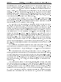
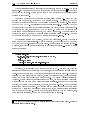
Figure 8.1:
"x:A"
"~p", "T", "F"
"p /\ q", "p \/ q"
"p ==> q"
"(!x y. P)"
"(!y::P. Q)"
"(?x y. P)"
"(?x::P. Q)"
"f x"
"(\x. E)"
"b => E1 | E2"
"{a,b}", "{f x | P x}"
"x IN V", "U SUBSET V"
"U UNION V", "U INTER V"
"U DIFF V"
"CONS a s", "SNOC a s"
"[a;b;c]", "APPEND s t"
The HOL Notation.
J
operations such as replacing an x at a particular position in a formula with something
else. On the other hand it does take quite before one gets a sucient grip on what
exactly each tool does, and how to use them eectively. Perhaps, this is one thing that
scares some potential users away.
Another problem is the collection of pre-proven facts. Although HOL is probably
a theorem prover with the richest collection of facts, compared to the knowledge of
a human expert, it is a novice. It may not know, for example, how come a nite
lattice is also well-founded, whereas for humans this is obvious. Even simple fact such
as (8a; b :: (9x :: ax + b x2)) may be beyond HOL knowledge. When a fact is
unknown, the user will have to prove it himself. Many users complain that their work
is slowed down by the necessity to 'teach' HOL various simple mathematical facts. At
the moment, various people are working on improving and enriching the HOL library
of facts. For example, for the purpose of proving the FSA algorithm we have also
produced libraries about well-founded relations, graphs, and lattices.
Having said all these, let us now take a closer at the HOL system.
8.1 Formulas in HOL
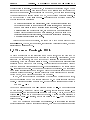
Figure 8.1 shows examples of how the standard notation is translated to the HOL
notation. As the reader can see, the HOL notation is as close an ASCII notation can
be to the standard notation.
Every HOL formula |from now on called HOL term| is typed. There are primitive
Page 168
Chapter 8.
MECHANICAL THEOREM PROVING WITH HOL
types such as ":bool" and ":nat", which can be combined using type constructors.
For example, we can have the product of type A and B : ":A#B"; functions from A to
B : ":A->B"; lists over A: ":A list"; and sets over A: ":A set". The user does not
have to supply complete type information as HOL is equipped with a type inference
system. For example, HOL can type the term "p ==> q" from the fact that ==> is
a pre-dened operator of type ":bool->bool->bool", but it cannot accept "x = y"
as a term without further typing information. All types in HOL are required to be
non-empty. A consequence of this is that dening a sub-type will require a proof of
the non-emptiness of the sub-type.
We can have type-variables to denote, as the name implies, arbitrary types. Names
denoting type-variables must always be preceded by a * like in *A or *B. Type variables
are always assumed to be universally quantied (hence allowing a limited form of
polymorphism). For example "x IN {x:*A}" is a term stating x is an element of the
singleton {x}, whatever the type of x is.
8.2 Theorems and Denitions
A theorem is, roughly stated, a HOL term (of type bool) whose correctness has been
proven. Theorems can be generated using rules. HOL has a small set of primitive rules
whose correctness has been checked. Although sophisticated rules can be built from
the primitive rules, basically using the primitive rules is the only way a theorem can
be generated. Consequently, the correctness of a HOL theorem is guaranteed. More
specically, a theorem has the form:
A1; A1; ... |- C
where the Ai's are boolean HOL terms representing assumptions and C is also boolean
HOL term representing the conclusion of the theorem. It is to be interpreted as: if all
Ai's are valid, then so is C. An example of a theorem is the following:
"P 0 /\ (!n. P n ==> P (SUC n)) |- (!n. P n)"
which is the induction theorem on natural numbers 1 .
As examples of (frequently used) rules are REWRITE_RULE and MATCH_MP. Given a list
of equational theorems, REWRITE_RULE tries to rewrite a theorem using the supplied
equations. The result is a new theorem. MATCH_MP implements the modus ponens
principle. Below are some examples of HOL sessions.
1
2
3
4
5
6
7
8
1
#DE_MORGAN_THM ;;
|- !t1 t2. (~(t1 /\ t2) = ~t1 \/ ~t2) /\ (~(t1 \/ t2) = ~t1 /\ ~t2)
#th1 ;;
|- ~(p /\ q) \/ q
#REWRITE_RULE [DE_MORGAN_THM] th1 ;;
|- (~p \/ ~q) \/ q
All variables which occur free are assumed to be either constants or universally quantied.
J
8.2.
THEOREMS AND DEFINITIONS
Page 169
The line numbers have been added for our convenience. The # is the HOL prompt.
Every command is closed by ;;, after which HOL will return the result. On line 1 we
ask HOL to return the value of DE_MORGAN_THM. HOL returns on line 2 a theorem, de
Morgan's theorem. Line 4 shows a similar query. On line 7 we ask HOL to rewrite
theorem th1 with theorem DE_MORGAN_THM. The result is on line 8.
The example below shows an application of the modus ponens principle using the
MATCH_MP rule.
1
2
3
4
5
6
7
8
#LESS_ADD ;;
|- !m n. n < m ==> (?p. p + n = m)
#th2 ;;
|- 2 < 3
#MATCH_MP LESS_ADD th2;;
|- ?p. p + 2 = 3
J
As said, in HOL we have access to the programming language ML. HOL terms and
theorems are objects in the ML world. Rules are functions that work on these objects.
Just as any other ML functions, rules can be composed like rule1 o rule2. We can
also dene a recursive rule:
letrec REPEAT_RULE b rule x =
if b x then REPEAT_RULE b rule (rule x) else x
The function REPEAT_RULE repeatedly applies the rule rule to a theorem x, until it
yields something that does not satisfy b. As can be seen, HOL is highly programmable.
In HOL a denition is also a theorem, stating what the object being dened means.
Because HOL notation is quite close to the standard mathematical notation, new objects can be, to some extend, dened naturally in HOL. Above it is remarked that
the correctness of a HOL theorem is, by construction, always guaranteed. The correctness is however relative to the axioms of HOL. While the latter have been checked
thoroughly, one can in HOL introduce additional axioms, and in doing so, one may
introduce inconsistency. Therefore adding axioms is a practice generally avoided by
HOL users. Instead, people rely on denitions. While it is still possible to dene something absurd, we cannot derive false from any denition. Below we show how things
can be dened in HOL.
1 #let HOA_DEF = new_definition
2
(`HOA_DEF`,
3
"HOA (p,a,q) =
4
(!(s:*) (t:*). p s /\ a s t ==> q t)") ;;
5
6 HOA_DEF = |- !p a q. HOA(p,a,q) = (!s t. p s /\ a s t ==> q t)
J
The example above shows how Hoare triples can be dened (introduced). Here, the
limitation of HOL notation begins to show up. We
denote a Hoare triple with fpg a fqg.
a
Or, we may even want to write it like this: p ,! q. A good notation greatly improves
Page 170
Chapter 8.
MECHANICAL THEOREM PROVING WITH HOL
the readability of formulas. Unfortunately, at this stage of its development, HOL does
not support fancy symbols. Formulas have to be typed linearly from left to right (no
stacked symbols or such). Inx operators can be dened, but that is as far as it goes.
This is of course not a specic problem of HOL, but of theorem provers in general. If
we may quote from Nuprl User's Manual |Nuprl is probably a theorem prover with
the best support for notations:
In mathematics notation is a crucial issue. Many mathematical developments
have heavily depended on the adoption of some clear notation, and mathematics
is made much easier to read by judicious choice of notation. However mathematical notation can be rather complex, and as one might want an interactive
theorem prover to support more and more notation, so one might attempt to
construct cleverer and cleverer parsers. This approach is inherently problematic.
One quickly runs into issues of ambiguity.
Notice that in the above denition, the s and the t have a polymorphic type of
. That is, they are states, functions from variables to values, whatever
'variables' and 'values' may be.
":*var->*val"
8.3 Theorem Proving in HOL
To prove a conjecture we can start from some known facts, then combine them to
deduce new facts, and continue until we obtain the conjecture. Alternatively, we can
start from the conjecture, and work backwards by splitting the conjecture into new
conjectures, which are hopefully easier to prove. We continue until all conjectures
generated can be reduced to known facts. The rst yields what is called a forward
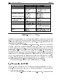
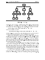
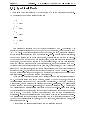
proof and the second yields a backward proof. This can illustrated by the tree in Figure
8.2. It is called a proof tree. At the root of the tree is the conjecture. The tree is said
to be closed if all leaves are known facts, and hence the conjecture is proven if we can
construct a closed proof tree. A forward proof attempts to construct such a tree from
bottom to top, and a backward proof from top to bottom.
In HOL, new facts can readily be generated by applying HOL rules to known facts,
and that is basically how we do a forward proof in HOL. HOL also supports backward
proofs. A conjecture is called a goal in HOL. It has the same structure as a theorem:
A1; A2; ... ?- C
Note that a goal is denoted with ?- whereas a theorem by |-. To manipulate goals
we have tactics. A tactic may prove a goal |that is, convert it into a theorem. For
example ACCEPT_TAC proves a goal ?- p if p is a known fact. That is, if we have the
theorem |- p, which has to be supplied to the tactic. A tactic may also transform a
goal into new goals |or subgoals, as they are called in HOL|, which hopefully are
easier to prove.
Many HOL proofs rely on rewriting and resolution. Rewrite tactics are just like
rewrite rules: given a list of equational theorems, they use the equations to rewrite
8.3.
THEOREM PROVING IN HOL
Page 171
g0
g1
g4
g5
g7
g8
g3
g2
g6
g9
g10
g11
g12
Figure 8.2:
J
A proof tree.
the right-hand side of a goal. A resolution tactic, called RES_TAC, tries to generate
more assumptions by applying, among other things, modus ponens to all matching
combinations of the assumptions. So, for example, if RES_TAC is applied to the goal:
"0<x"; "!y. 0<y ==> z<y+z"; "z<x+z ==> p"
?-
"p"
will yield the following new goal:
"z<x+z"; "0<x"; "!y. 0<y ==> z<y+z"; "z<x+z ==> p"
?-
"p"
Applying RES_TAC to the above new goal will generate "p" and the tactic will then
conclude that the goal is proven, and return the corresponding theorem.
Tactics are not primitives in HOL. They are built from rules. When applied to a
goal ?- p, a tactic generates not only new goals |say, ?- p1 and ?- p2| but also
a justication function. Such a function is a rule, which if applied, in this case, to
theorems of the form |- p1 and |- p2 will produce |- p. When a composition of
tactics proves a goal, what it does is basically re-building the corresponding proof tree
from the bottom, the known facts, to the top using the generated justication functions
to construct new facts along the tree.
HOL provides much better support for backward proofs. For example, HOL provides tactics combinators, also called tacticals. For example, if applied to a goal,
tac1 THEN tac2 will apply tac1 rst then tac2; tac1 ORELSE tac2 will try to apply
tac1, if it fails tac2 will be attempted; and REPEAT tac applies tac until it fails. On
the other hand, no rules combinators are provided. Of course, using the meta language
ML it is quite easy to make rules combinators.
HOL also provides a facility, called the sub-goal package, to interactively construct
a backward proof. The package will memorize the proof tree and justication functions
generated in a proof session. The tree can be displayed, extended, or partly un-done.
Page 172
Chapter 8.
MECHANICAL THEOREM PROVING WITH HOL
1 #set_goal ([],"!s. MAP (g:*B->*C) (MAP (f:*A->*B) s) = MAP (g o f) s");;
2 "!s. MAP g(MAP f s) = MAP(g o f)s"
3
4 #expand LIST_INDUCT_TAC ;;
5 2 subgoals
6 "!h. MAP g(MAP f(CONS h s)) = MAP(g o f)(CONS h s)"
7
1 ["MAP g(MAP f s) = MAP(g o f)s" ]
8
9 "MAP g(MAP f[]) = MAP(g o f)[]"
10
11 #expand ( REWRITE_TAC [MAP]);;
12 goal proved
13 |- MAP g(MAP f[]) = MAP(g o f)[]
14
15 Previous subproof:
16 "!h. MAP g(MAP f(CONS h s)) = MAP(g o f)(CONS h s)"
17
1 ["MAP g(MAP f s) = MAP(g o f)s" ]
18
19 #expand (REWRITE_TAC [MAP; o_THM]);;
20"!h. CONS(g(f h))(MAP g(MAP f s)) = CONS(g(f h))(MAP(g o f)s)"
21 1 ["MAP g(MAP f s) = MAP(g o f)s" ]
22
23 #expand (ASM_REWRITE_TAC[]);;
24 goal proved
25 . |- !h. CONS(g(f h))(MAP g(MAP f s)) = CONS(g(f h))(MAP(g o f)s)
26 . |- !h. MAP g(MAP f(CONS h s)) = MAP(g o f)(CONS h s)
27 |- !s. MAP g(MAP f s) = MAP(g o f)s
28
29 Previous subproof:
30 goal proved
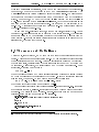
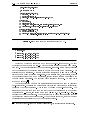
Figure 8.3:
An example of an interactive backward proof in HOL.
J
Whereas interactive forward proofs are also possible in HOL simply by applying rules
interactively, HOL provides no facility to automatically record proof histories (proof
trees). To prove a goal A ?- p with the package, we initiate a proof tree using a
function called set_goal. The goal to be proven has to be supplied as an argument.
The proof tree is extended by applying a tactic. This is done by executing expand tac
where tac is a tactic. If the tactic solves the (sub-) goal, the package will report it,
and we will be presented with the next subgoal which still has to be proven. If the
tactic does not prove the subgoal, but generates new subgoals, the package will extend
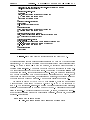
the proof tree with these new subgoals. An example is displayed in Figure 8.3.
We will try to prove g (f s) = (g f ) s for all lists s, where the map operator
is dened as: f [] = [] and f (a; s) = (f:a); (f s). In HOL f s is denoted by
MAP f s. The tactic LIST_INDUCT_TAC on line 4 applies the list induction principle,
splitting the goal according to whether s is empty of not. This results two subgoals
listed on lines 6-9. The rst subgoal is at the bottom, on line 9, the second on line 6-7.
If any subgoal has assumptions they will be listed vertically. For example, the subgoal
on lines 6-7 is actually:
"MAP g(MAP f s) = MAP(g o f)s"
?- "!h. MAP g(MAP f(CONS h s)) = MAP(g o f)(CONS h s)"
8.3.
THEOREM PROVING IN HOL
Page 173
The next expand on line 11 is applied to rst subgoal, the one on line 9. The tactic
REWRITE_TAC [MAP] attempts to do a rewrite using the denition of MAP 2 and succeeds
in proving the subgoal. Notice that on line 13 HOL reports back the corresponding
theorem it just proven.
Let us now continue with the second subgoal, listed on line 6-7. Since the rst
subgoal has been proven, this is now the current subgoal. On line 19, we try to
rewrite the current subgoal with the denition of MAP and a theorem o_THM stating
that (g f )x = g(fx). This results in the subgoal in line 20-21. On line 23 we try to
rewrite the right hand side of the current goal (line 20) with the assumptions (line 21).
This proves the goal, as reported by HOL on line 24. On line 29 HOL reports that
there are no more subgoals to be proven, and hence we are done. The nal theorem is
reported on line 27, and can be obtained using a function called top_thm. The state
of the proof tree at any moment can be printed using print_state.
The resulting theorem can be saved, but not the proof itself. Saving the proof is
recommended for various reasons. Most importantly, when it needs to be modied,
we do not have to re-construct the whole proof. We can collect the applied tactics |
manually, or otherwise there are also tools to do this automatically| to form a single
piece of code like:
let lemma = TAC_PROVE
(([],"!s. MAP (g:*B->*C) (MAP (f:*A->*B) s) = MAP (g o f) s"),
LIST_INDUCT_TAC
THENL
[ REWRITE_TAC [MAP] ;
REWRITE_TAC [MAP; o_THM] THEN ASM_REWRITE_TAC ])
J
Sometimes, it is necessary to do forward proving in HOL. For example, there are
situations where forward proofs seem very natural, or if we are given a forward proof to
verify. It would be nice if HOL provides better support for forward proving. During our
research we have also written a package, called the LEMMA package, to automatically
record the whole proof history of a forward proof. The history consists basically of
theorems. It is implemented as a list instead of a tree, however a labelling mechanism
makes sure that any part of the history is readily accessible. Just as with the subgoal
package, the history can be displayed, extended, or partly un-done. The package also
allows comments to be recorded. The theorems in the history can each be proven using
ordinary HOL tools such as rules and tactics (that is, the LEMMA package is basically
only a recording machine). There is a documentation included with the package, else,
if the reader is interested, he can nd more information in [Pra93].
2
The name of the theorem dening the constant MAP happens to have the same name. These two
really refer to dierent things.
MAPs
Page 174
Chapter 8.
MECHANICAL THEOREM PROVING WITH HOL
8.3.1 Equational Proofs
A proof style which is overlooked by the standard HOL is the equational proof style.
An equational proof has the following format:
v
=
v
v
E0
E1
E2
En
f hint g
f hint g
f hint g
f hint g
Each relation Ei is related to Ei+1 by either the relation v or =. The relation v is
usually a transitive relation so that at the end of the derivation, we can conclude that
E0 v En holds. Equational proofs are used very often. In fact, all proofs presented
in this thesis are constructed from equational sub-proofs. For low level applications,
in which one relies more on automatic proving, proof styles are not that important.
When dealing with a proof at a more abstract level, where less automatic support can
be expected, and hence one will have to be more resourceful, what one does is usually
write the proof on paper using his most favorite style, and then translate it to HOL.
Styles such as the equational proof style does not, unfortunately, t very well in the
standard HOL styles (that is, forward proofs using rules and backward proofs using the
subgoal package). So, either one has to adjust himself with the HOL styles |which is
not very encouraging for newcomers, not to mention that this oends the principle of
user friendliness| or we should provide better support.
There are two extension packages that will enable us to write equational proofs in
HOL. The rst is called the window package, written by Grundy [Gru91], the other is
the DERIVATION package which we wrote during our research. The window package is
more exible, namely because it is possible to open sub-derivations. The DERIVATION
package does not support sub-derivations, but it is much easier to use. The structure
and presentation of a DERIVATION proof also mimics the pen-and-paper style better.
The distinctions are perhaps rooted in the dierent purposes the authors of the packages
had in mind. The window package was constructed with the idea of transforming
expressions. It is the expressions being manipulated that are the focus of attention.
The DERIVATION package is written specically to mimic equational proofs in HOL.
Not only the expressions are important, but the whole proof, including comments, and
its presentation format.
A proof using the DERIVATION package has the following format:
8.3.
THEOREM PROVING IN HOL
1
2
3
4
5
6
7
8
9
10
11
12
13
14
15
16
17
18
19
20
ADD_TRANS ("<",LESS_TRANS)
BD "<" "(x*x) + x" ;;
DERIVE ("=:num->num->bool",
"(x+1)*x",
`* distributes over +`,
REWRITE_TAC [RIGHT_ADD_DISTRIB; MULT_LEFT_1 ]) ;;
DERIVE ("<",
"(x+1)*(x+1)",
`monotonicity of *`,
(CONV_TAC o DEPTH_CONV) num_CONV THEN ONCE_REWRITE_TAC [ADD_SYM]
THEN REWRITE_TAC [ADD; LESS_MULT_MONO; LESS_SUC_REFL]) ;;
DERIVE ("=:num->num->bool",
"(x*x) + (2*x) +1",
`* distributes over +`,
REWRITE_TAC [RIGHT_ADD_DISTRIB; LEFT_ADD_DISTRIB; MULT_LEFT_1; MULT_RIGHT_1;
TIMES2; ADD_ASSOC]) ;;
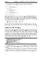
Figure 8.4:
1
2
3
4
5
6
Page 175
An example of an equational proof in HOL.
J
BD Rel E_0 ;;
DERIVE (Rel, E_1, Hint_1, Tac_1) ;;
DERIVE (= , E_1, Hint_2, Tac_2) ;;
...
DERIVE (Rel, E_n, Hint_n, Tac_n) ;;
J
Notice how the format looks very much like the pen-and-paper format. The only
additional components are the Tac i which are tactics required to justify each derivation step. The proof is initialized by the function BD. It sets E 0 as the begin expression
in the derivation and the relation Rel is to be used as the base of the derivation. This
relation has to be transitive. A theorem stating the transitivity of Rel has to be explicitly announced using a function ADD TRANS. Every DERIVE step, if successful, extends
the derivation history with a new expression, related either with Rel or equality with
the last derived expression. The supplied hint will also be recorded. An example is
shown in Figure 8.4 3 .
The tactics required to prove the DERIVE steps are usually not easy to construct
non-interactively. Therefore the package also provides some functions to interactively
construct the whole derivation. This is done by calling the sub-goal package. The
DERIVE package will take care that the right goal that corresponds to the current
derivation step |that is, something of the form ?- Rel E_i E_j or ?- E_i = E_j|
is passed to the subgoal package. The tactic required to prove the derivation step can
be constructed using the subgoal package. When the step is proven, the newly derived
expression is automatically added to the derivation history.
3
The proof in Figure 8.4 is not the shortest possible proof, but it will do for the purpose here.
Page 176
Chapter 8.
MECHANICAL THEOREM PROVING WITH HOL
The derivation in Figure 8.4 corresponds to the following derivation:
xx+x
= f distributes over + g
(x + 1) x
< f monotonicity of g
(x + 1) (x + 1)
= f distributes over + g
x x + 2x + 1
from which we conclude x x + x < x x + 2x + 1. The derivation generated by a
DERIVATION package can be printed at any time using the function DERIVATION. For
example, if the code in Figure 8.4 is executed, calling DERIVATION will generate an
output like the nicely printed derivation above, except that it is in the ASCII format.
The conclusion of the derivation, that is the theorem
|- ((x*x) + x) < ((x*x) + (2*x) + 1)
can be obtained using a function called ETD (which abbreviates Extract Theorem from
Derivation). A complete manual of the package can be found along with the package.
8.4 Automatic Proving
As the higher order logic |the logic that underlies HOL| is not decidable, there exists
no decision procedure that can automatically decide the validity of all HOL formulas.
However, for limited applications, it is often possible to provide automatic procedures.
The standard HOL package is supplied with a library called arith written by Boulton
[Bou94]. The library contains a decision procedure to decide the validity of a certain
subset of arithmetic formulas over natural numbers. The procedure is based on the
Presburger natural number arithmetic [Coo72]. Here is an example:
1
2
3
4
5
6
#set_goal([],"x<(y+z) ==> (y+x) < (z+(2*y))") ;;
"x < (y + z) ==> (y + x) < (z + (2 * y))"
#expand (CONV_TAC ARITH_CONV) ;;
goal proved
|- x < (y + z) ==> (y + x) < (z + (2 * y))
J
We want to prove x < y + z ) y + x < z + 2y. So, we set the goal on line 1.
The Presburger procedure, ARITH CONV, is invoked on line 4, and immediately prove
the goal.
There is also a library called taut to check the validity of a formula from proposition
logic. For example, it can be used to automatically prove p ^ q ) :r _ s = p ^ q ^
r ) s, but not to prove more sophisticated formulas from predicate logic, such as
8.4.
AUTOMATIC PROVING
Page 177
(8x :: P:x) ) (9x :: P:x) (assuming non-empty domain of quantication). There is a
library called faust written by Schneider, Kropf, and Kumar [SKR91] that provides
a decision procedure to check the validity of many formulas from rst order predicate
logic. The procedure can handle formulas such as (8x :: P:x) ) (9x :: P:x), but not
(8P :: (8x : x < y : P:x) ) P:y) because the quantication over P is a second order
quantication (no quantication over functions is allowed). Here is an example:
1
2
3
4
5
6
7
8
9
10
11
12
13
14
#set_goal([], "HOA(p:*->bool,a,q) /\ HOA (r,a,s)
==>
HOA (p AND r, a, q AND s)") ;;
"HOA(p,a,q) /\ HOA(r,a,s) ==> HOA(p AND r,a,q AND s)"
#expand(REWRITE_TAC [HOA_DEF; AND_DEF] THEN BETA_TAC) ;;
"(!s t. p s /\ a s t ==> q t) /\ (!s t. r s /\ a s t ==> s t) ==>
(!s t. (p s /\ r s) /\ a s t ==> q t /\ s t)"
#expand FAUST_TAC ;;
goal proved
|- (!s t. p s /\ a s t ==> q t) /\ (!s t. r s /\ a s t ==> s t) ==>
(!s t. (p s /\ r s) /\ a s t ==> q t /\ s t)
|- HOA(p,a,q) /\ HOA(r,a,s) ==> HOA(p AND r,a,q AND s)
In the example above, we try to prove one of the Hoare triple basic laws, namely:
J
fpg a fqg ^ frg s fsg
fp ^ rg a fq ^ sg
The goal is set on line 1-3. On line 6 we unfold the denition of Hoare triple and the
predicate level ^, and obtain a rst order predicate logic formula. On line 10 we invoke
the decision procedure FAUST TAC, which immediately proves the formula. The nal
theorem is reported by HOL on line 14.
So, we do have some automatic tools in HOL. Further development is badly required
though. The arith library cannot, for example, handle multiplication 4 and prove, for
example, (x + 1)x < (x + 1)(x + 1). Temporal properties of a program, such as we are
dealing with in UNITY, are often expressed in higher order formulas, and hence cannot
be handled by faust. Early in the Introduction we have mentioned model checking, a
method which is widely used to verify the validity of temporal properties of a program.
There is ongoing research that aims to integrate model checking tools with HOL 5 . For
example, Joyce and Seger have integrated HOL with a model checker called Voss to
check the validity of formulas from a simple interval temporal logic [JS93].
In general, natural number arithmetic is not decidable if multiplication is included. So the best
we can achieve is a partial decision procedure.
5 That is, the model checker is implemented as an external program. HOL can invoke it, and then
declare a theorem from the model checker's result. It would be safer to re-write the model checker
within HOL, using exclusively HOL rules and tactics. This way, the correctness of its results is
guaranteed. However this is often less ecient, and many people from circuit design |which are
inuential customers of HOL| are, understandably, quick to reject less ecient product.
4