Download Strut Fixtures

STRUT FIXTURES:
MODULAR SYNTHESIS AND EFFICIENT ALGORITHMS
by
Richard Jeffery Wagner
A Dissertation Presented to
THE FACULTY OF THE GRADUATE SCHOOL
UNIVERSITY OF SOUTHERN CALIFORNIA
In Partial Fulfillment of the
Requirements for the Degree
DOCTOR OF PHILOSOPHY
(Computer Science)
December 1997
Copyright 1997
Richard Jeffery Wagner
Table of Contents
1. Introduction .............................................................................................2
2. Related Work..........................................................................................5
2.1 Minimalism Related Work ..................................................................7
2.2 Grasping Related Work .....................................................................8
2.3 Fixturing Related Work ....................................................................10
2.3.1 Friction .......................................................................................10
2.3.2 Form Closure .............................................................................11
2.3.3 Modular Fixturing .......................................................................12
2.4 Fixture Loading Related Work .........................................................16
2.4.1 Fixture Loading Planning ...........................................................17
3. Modular Fixturing in the Plane ..............................................................19
3.1 The Brost-Goldberg Algorithm .........................................................19
3.2 Personal Computer Implementation ................................................20
3.2.1 Part Transformation ...................................................................24
3.2.2 Fast Test for Form Closure........................................................25
3.2.3 Quality Metrics ...........................................................................25
4. FixtureNet .............................................................................................28
4.1 Summary .........................................................................................28
4.2 Web Access ....................................................................................28
4.3 Algorithm .........................................................................................28
4.4 Architecture .....................................................................................30
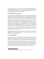
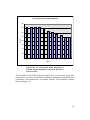
4.5 Usage Statistics ...............................................................................36
4.6 FixtureNet II .....................................................................................37
4.7 FixtureNet III ....................................................................................37
4.7.1 Features ....................................................................................40
4.7.2 Classes ......................................................................................41
4.7.3 Using FixFun2D .........................................................................42
ii
5. Modular Fixturing in 3D Space .............................................................44
5.1 Parts Modeled as Sets of Facets.....................................................46
5.2 Modular Strut Hardware Primitives ..................................................47
5.3 Algorithm .........................................................................................48
5.3.1 Form Closure Test .....................................................................58
5.3.2 Quality Metrics ...........................................................................59
5.4 Computational Complexities of Syntheses ......................................64
5.4.1 Complete Synthesis...................................................................64
5.4.2 Heuristic Synthesis ....................................................................66
5.5 Fixturability of Parts Using Struts.....................................................70
5.6 General Frictionless Fixturability......................................................72
5.6.1 Candidate Facet Sets ................................................................73
5.6.2 2D Test for FG ...........................................................................87
5.6.3 3D Test for FG ...........................................................................90
5.7 Facet Set Analysis ...........................................................................90
5.7.1 Necessary Facet Set Analysis ...................................................90
5.7.2 Sufficient Facet Set Analysis .....................................................97
5.8 Constructive Fixture Synthesis Algorithm ......................................103
5.8.1 Approach .................................................................................103
5.8.2 Results ....................................................................................105
5.9 Complexity Attack via Quality Metrics ............................................113
5.10 Design for Fixturing .....................................................................114
6. A Taxonomy of Modular Fixture Systems ...........................................115
6.1 1D Fixtures ....................................................................................115
6.2 Appropriate Discretizations for Fixture Schemes ...........................117
6.2.1 2D Fixtures ..............................................................................117
6.2.2 3D Fixtures ..............................................................................119
7. Strut Fixture Loading ..........................................................................121
7.1 3D Fixture Loading Planning .........................................................121
iii
7.1.1 Strut Fixture Loading ...............................................................121
7.1.2 Strut Fixture Loading Implementation ......................................125
8. Accessibility Metric .............................................................................127
8.1 Accessibility of a Point ...................................................................127
8.2 Accessibility of a Facet ..................................................................128
8.3 Implementation ..............................................................................128
9. Conclusion ..........................................................................................130
9.1 Summary of Major Contributions ...................................................130
9.1.1 Two Dimensional Fixtures .......................................................130
9.1.2 Three Dimensional Fixtures.....................................................131
9.1.3 Facet Set Analysis ...................................................................132
9.1.4 Constructive Strut Fixture Synthesis Algorithm .......................132
9.2 Summary of Minor Contributions ...................................................132
9.2.1 Complexity Attack Refutation ..................................................132
9.2.2 Accessibility Metric ..................................................................132
9.2.3 Fixture Loading ........................................................................133
9.3 Future Work...................................................................................133
9.3.1 Extension to Curved Parts .......................................................133
9.3.2 NFS Enumeration ....................................................................138
9.3.3 Stochastic SFS Computation...................................................138
9.3.4 Variable Pose Synthesis..........................................................138
9.3.5 Extensions to Java FixtureNet .................................................139
10. Acknowledgments ............................................................................140
11. References .......................................................................................141
iv
Table of Figures
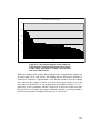
Figure 1.1: Typical commercial off-the-shelf modular fixturing toolkit
components. ...............................................................................................3
Figure 1.2: Dissertation topic relationship map. .........................................4
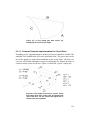
Figure 3.1: The USC 2D Fixturing Program handles arbitrary
polygons. ..................................................................................................20
Figure 3.2: The “Aluminum Bracket” is shown in the part drawing
tool. The stay-out zone is shown in red. ...................................................22
Figure 3.3: During fixture computation, the part is grown by the fixel
radius. The stay-out zone is also grown. Notice how the stay-out
zone incorporates the curve of the fixel. This is necessary should a
grown part edge intersect a corner of the stay-out zone. .........................23
Figure 3.4: The completed fixture set has 151 elements. The best
fixture has a quality metric of 1.0 and all the rest have lower
rankings. This particular metric prefers fixtures that resist both inplane forces in all directions and in-plane torques in both directions. ......24
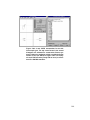
Figure 3.5: The quality metric options are accessed via pull-down
menus.......................................................................................................26
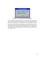
Figure 3.6: The custom quality metric dialog window. ..............................27
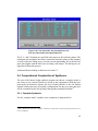
Figure 4.1: The USC 2D fixturing program is shown running in
slave mode as part of FixtureNet. Note that the menus are grayed
out and not accessible to a user. The request ID being serviced is
shown at the bottom. ................................................................................29
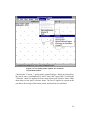
Figure 4.2: FixtureNet system architecture. ..............................................30
Figure 4.3: If more than zero fixtures are found for the part,
FixtureNet offers to display the best four. .................................................32
Figure 4.4: The four best solutions (fixture configurations) for the
hook-shaped part. The default quality metric is formulated to resist
several generic combinations of forces and moments. ............................34
Table 4.1: FixtureNet Statistics.................................................................36
Figure 4.5 The part is drawn in the smaller upper window in
FixtureNet III. Stay-out zones are shown in red. The grown part and
stayout zones are then shown in the fixture display window during
fixture synthesis. .......................................................................................38
v
Figure 4.6: When fixture synthesis is complete, the fixtures are
displayed in the fixture display window. ....................................................39
Table 4.2: Fixture2D Applet Classes ........................................................41
Figure 4.7: Fixture2D Applet Classes Relationships ................................42
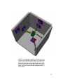
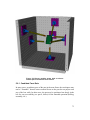
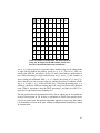
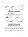
Figure 5.1: Rectangular lattices of holes cover the walls of the
fixturing frame (box). The holes are spaced on one-inch centers,
but the half-inch spacing of the holes on the strut base plates gives
a virtual box grid pitch of two holes per inch. Seven struts hold the
eleven-faceted polyhedral part in form closure. ........................................45
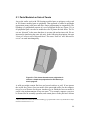
Figure 5.2: This eleven-faceted convex polyhedron is used as a
simple test polyhedron for the fixture synthesis program. ........................46
Figure 5.3: The electric staple gun is modeled as a set of directed
facets ........................................................................................................47
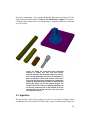
Figure 5.4: Struts are constructed from cylindrical sections of length
one, two, and four inches, screwed together with threaded studs
(not shown), with a screw-adjustable ball end, and mounted to a
base consisting of a base plate, a turret, and a pivot. The pivot and
turret have indicators for setting their angles by calibration marks
scribed on the turret and base plate. Angle is set to the nearest
degree. The length of the strut is set to the nearest thousandth of
an inch by measuring with a dial indicator from the hexagonal
section of the ball end to the end of the last cylindrical section. ...............48
Figure 5.5: Available grid densities. Doubling linear pitch with each
iteration quadruples the density. The hardware prototype will
support a pitch maximum of two per inch. ................................................49
Figure 5.6: A part facet is shown projected onto the virtual grid wall.
The virtual wall is a plane parallel to and one inch inside the
physical box wall. ......................................................................................50
Figure 5.7: Nodes (points, shown here as circles) on the virtual wall
that are inside the facet projection. ..........................................................51
Figure 5.8: One point is deleted in this example of the “convex hull”
heuristic. The remaining points are “on” the convex hull of the
original set of points. ................................................................................52
vi
Figure 5.9: The two nodes most distant from each other are
retained in the “most distant” (two strut) heuristic. It might also be
beneficial to use a “most distant triple” (three strut) heuristic, but
the “most distant pair” was found to work quite well. ................................52
Figure 5.10: The 3D strut fixturing program main window shows
three orthogonal views of the loaded part model. .....................................54
Figure 5.11: When the computation is complete, the best fixture is
displayed in orthogonal projection, with line segments symbolizing
the struts, with the fixture grid also displayed. ..........................................55
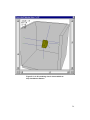
Figure 5.12: A 3D rendering view is also available to help visualize
the fixtures. ...............................................................................................56
Figure 5.13: 28 fixtures were found for the 40-facet stapler using
the program defaults (2-strut heuristic and 24 strut regular pruning
level). ........................................................................................................57
Figure 5.14: 3D perspective view of the first (best) stapler strut
fixture. .......................................................................................................58
Figure 5.15: Application of a clamping force results in form closure
on the left. Applying the force shown on the right will result in the
block rotating counterclockwise and pulling away from the top fixel.
If the block were “glued” to the top fixel, a negative reaction force
would be generated. My form closure test does that computation,
rejecting the configuration on the right. ....................................................59
Figure 5.16: When an external force is applied to the fixtured part,
reaction forces are generated at the contact points (shown in blue).
The fixture on the left is “good” by the generic quality metric, while
the one on the right is not as good. ..........................................................60
Figure 5.17: The user-defined quality metric dialog window allows
the user to enter up to three wrenches. Any possible combination
of static loads on a rigid body can be reduced to at most three
wrenches. The bi-directional option also calculates reactions for the
reversed loads. .........................................................................................61
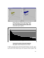
Figure 5.18: Fixture quality (using the generic quality metric) of the
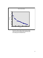
eleven-faceted part as a function of fixture ordering for the 92
fixtures found. ...........................................................................................62
Figure 5.19: Fixture quality (using the generic quality metric) of the
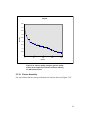
stapler as a function of fixture ordering for 200 fixtures found. .................63
vii
Figure 5.20: The technician who assembles the fixture can print out
the strut specification list. .........................................................................64
Figure 5.21: The part on the left is “immobilized,” but it is of the
very poorest quality as a “fixture.” If the fixels are moved away from
the centers of the edges, the fixture quality is improved
dramatically. .............................................................................................68
Figure 5.22: The four inch cube is fixtured in a four-sided virtual
fixture box. ................................................................................................71
Figure 5.23 Seven modular struts hold an eleven-faceted part in
frictionless form closure. ...........................................................................73
Figure 5.24: Any frictionless fixture for this pyramid-shaped part will
require a fixel on the octagonal base. Hence, the base is a
necessary facet subset (SNFS) with one member. ..................................75
Figure 5.25: Any fixture for this polyhedral part will require a fixel on
one or more of the eight members of the SNFS. ......................................76
Figure 5.26: This edge set has three directed edges, E1, E2, and
E3. The arrows indicate the outer (fixture interface) side of the
edges. It has three strong necessary edge (facet) subsets, each
with one element. .....................................................................................77
Figure 5.27: This edge set likewise has three SNFSs, one with two
elements. If SNFS3 is removed from the edge set, the remaining
subset is not FG. Replace either E1 or E4 and the result is FG. ..............77
Figure 5.28: The remaining edge set, {E1, E2} is not FG. ........................78
Figure 5.29: This edge set has weak necessary edge (facet)
subsets. ....................................................................................................78
Figure 5.30: An octagon, P, illustrates the dot product heuristic in
two dimensions. The eight edges of P and their direction vectors
are shown. ................................................................................................80
Table 5.1: Shown as a table here, the dot products of every pair of
edges (for the 2D example, facets for a part) are computed and
stored as a sorted list. ..............................................................................81
Figure 5.31 ...............................................................................................83
Figure 5.32 ...............................................................................................84
viii
Figure 5.33: These three facets close direction space in the plane.
Three facets (edges) in 2D close rotation space if their projections
have a common volume. ..........................................................................87
Figure 5.34: Any facet can be moved in its normal direction and
form an equivalent facet set from the standpoint of fixturability.
Hence, any facet represents an equivalence class of facets. ...................88
Figure 5.35: The wrench triple on the left is a “plus” (CCW) cyclic
triple. The middle is a minus triple. The triple on the right is not
cyclic. ........................................................................................................88
Figure 5.36: The edge set on the left has force direction and
rotation closure, hence there exists a fixture for it (center). Moving
one edge (right) shows that rotation closure is lost when the edge
no longer participates in a “minus pair.” ...................................................89
Figure 5.37: Edges a and c are a “plus pair.” In both directions,
going from a to c and from c to a, theta is greater than phi. Other
possible pairs are minus pairs and odd pairs. If a 4-edge set spans
force space and contains both a plus and a minus edge pair, then
the edge set is fixturable...........................................................................89
Figure 5.38: The facet set analysis Window. If the analysis of the
SNFSs is complete, as in this case, the union of the SNFSs will be
fixturable (have FG). Elapsed time is shown in seconds. .........................91
Figure 5.39: The 3D view of the NFSs found by the analysis. Each
NFS is shown in a different color. Any fixture for the 11-faceted part
must incorporate at least one facet from each of the three NFSs.
This facet subset (the union of the NFSs) has fewer members than
the input part, but it too has FG. ...............................................................92
Figure 5.40: The NFSs of the cube, the regular octahedron, the
concave part, and the cube with one face replaced with two
coplanar faces. All these NFS enumerations are complete and
correct. .....................................................................................................93
Figure 5.41: The unit direction vector endpoint space forms the
surface of a sphere. Direction vector dot products with a given
direction (A in this case) form equivalence class bands like the lines
of latitude. Hence, a vector pointing in the opposite direction as D
will be in the same dot product equivalence class in 3D. This is why
the simple dot product heuristic breaks down in 3D. However, doing
the heuristic three times for each of three orthogonal 2D projections
revives this approach. ...............................................................................94
ix
Figure 5.42: The two (incompletely defined) NFSs for the 40-facet
electric stapler took only 37 seconds to identify using the
orthogonally re-sorted dot product heuristic and “weakly defined”
NFSs. The complete version of the algorithm would take many
years to finish. The facets shown in blue comprise an SNFS. .................95
Figure 5.43: The 100-facet randomly generated set faces are in the
locus of the surface of a sphere. The part is loaded into the
program main window, left, and the two identified NFSs are shown
in green and blue on the right. This illustrates graphically how the
heuristic NFS analysis breaks down for large facet sets. Dividing a
spherical set into two hemispheres does not give insight into fixture
construction. .............................................................................................96
Figure 5.44: Complete SFS enumeration for the 11-facet part. The
top seven facets in the sorted histogram are selected as a sufficient
facet set for fixture construction. Notice that this set is identical to
the union of the SNFSs (bottom right). .....................................................98
Figure 5.45: The 11-facet part sorted histogram. In any SFS
analysis histogram, every facet will have a non-zero count. .....................99
Figure 5.46: 4 and 5-SFS enumeration for the 40-facet staple gun.
The top seven facets in the sorted histogram are selected for
constructive fixture synthesis. Notice the similarity of this set with
the facets shown in blue (an SNFS) of Figure 5.42. This analysis
took 1585 seconds (nearly half an hour) on a Pentium Pro 200
MHz machine..........................................................................................100
Figure 5.47: The sorted histogram for the stapler for 5-SFS
analysis. Six facets stand out as having significantly higher
participation in SFSs. The time limit was set to 1000 seconds. ..............101
Figure 5.48: Left: a 3D view of the top six facets in the sorted
histogram for the electric stapler, identified by the SFS analysis
algorithm. Right: these same six facets were identified as the
smallest SNFS with the NFS analysis algorithm. ....................................102
Figure 5.49: The ordering of the sorted histogram is not changed
for the first six facets for the faster 4-SFS analysis. The time limit
was set to 10 seconds. ...........................................................................102
Figure 5.50: The constructive fixture synthesis program defaults to
a “quick” analysis (bypassing the SFS analysis) which sorts the
facets by size (larger first) and then takes the first 7-SFS found.
This is the construction 7-SFS for 11-facet part. ....................................106
x
Figure 5.51: After the quick analysis, the fixture is constructed by
rotating the part so that the facet with the direction farthest from the
average direction projects to the outer corner of the left box wall.
This fixture construction took only 2.7 seconds (versus several
minutes for the complete optimal (specified pose) fixture synthesis). ....107
Figure 5.52: The constructed fixture shown as a 3D schematic.
Notice the facet pointing to the outer corner of the left wall that
used to point to open sky. ......................................................................108
Figure 5.53: The three orthogonal views of the regular octahedron
are identical. ...........................................................................................109
Figure 5.54: The octahedron was fixtured in 2.4 seconds on a
Pentium Pro 200. ....................................................................................110
Figure 5.55: No constructive fixture for the staple gun was found.
The program reported failure in under a second on the Pentium Pro
200. The stapler is fairly large for the fixture box, and the existing
algorithm causes some of the facets to move out of the box as a
result of translation and rotation. ............................................................111
Figure 5.56: When the stapler is scaled to 7/10 its original size, a
fixture is constructed for it in 53 seconds. ..............................................112
Table 5.2: Comparison of execution times for the pose-specific
(with 2-strut heuristic) and variable pose (constructive) algorithms
for several different parts. .......................................................................112
Figure 7.1: The staple gun facets are projected onto the fixture box
walls during fixture synthesis computation. Because the box has a
floor but no ceiling, generally, more up-pointing candidate struts will
be found than down-pointing ones. ........................................................122
Figure 7.2: This fixture is top-loadable. Three struts have directions
not pointing up, and four struts have up components. To show that
the staple gun is gravity stable on the four up-pointing struts, the
horizontal CG of the part is tested against the horizontal convex
hull of the contact points. If the CG is within the convex hull, the
part will be stable and may be released after it is placed in position. .....124
Figure 7.3: The three non-up pointing struts are removed and the
stapler is moved in a vertical trajectory into contact with the four uppointing struts. ........................................................................................126
xi
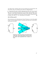
Figure 8.1: The accessibility of a point on a planar surface is
quantified by the minimum angle to the surface normal from any of
several obstacles. Here, for point a, angle alpha is the minimal
angle to the surface normal and is described by a vertex of the
second obstacle. In 3D, this is a cone. ...................................................128
Figure 8.2: Facet accessibility analysis is run for two poses of the
11-faceted part. The accessibilities of the facets for the part located
toward the back of the box are shown in the upper half of the
window on the right. Then the part is translated eight inches
forward in the box (left). Those accessibilities are shown in the
lower half of the window on the right. The most accessible facet is
drawn in green (left)................................................................................129
Figure 9.1: A very simple part with convex (A), straight (B), and
concave (C) edges .................................................................................134
Figure 9.2: The simple curved part is “grown” by the fixel radius
(0.25 inch, in this case) by changing the radii of the arcs. The arc
centers and angles are invariant under this operation. ...........................134
Figure 9.3: One possible planar fixture for the simple curved part.
The clamp is represented by the rectangular piece with the
rounded end. ..........................................................................................135
Figure 9.4: A simple 2D part is in one contact configuration with
three circular fixels in this simulation in 2D Toy Box running in
Windows 95. ...........................................................................................136
Figure 9.5: The same simple part is shown in its second
configuration against the three fixels. .....................................................137
xii
Abstract
This dissertation focuses on modular fixture synthesis, and touches
on the design of modular fixturing systems and fixture loading. Efficient algorithms for synthesis of fixtures are made possible by
minimizing the set of fixture elements. The benefits of simple
modular systems include precision, rapid setup, reusability of
hardware and software components, and reduced computational
complexity.
Efficient algorithms for computational synthesis of modular fixtures and fixture loading planning exist and can be demonstrated
on inexpensive personal computers (Intel-Microsoft) if fixture
hardware primitives are designed to minimize complexity. Many of
these algorithms have been implemented. My contribution builds
on existing algorithms to extend their capability and introduces
some new related techniques, including WWW browser interfaces.
Key insights include strut fixture hardware primitives, enumerating
part facet subsets necessary and sufficient for frictionless fixturing,
and utilizing sufficient facet subsets in variable pose fixture synthesis. Those results are reported and directions for future research
are described.
1
1. Introduction
Efficient algorithms for computational design of modular fixtures1 and fixture
loading planning exist and can be demonstrated on inexpensive personal computers. Automated assembly operations require that parts and subassemblies be held
in fixtures while robots perform operations on them [[3]]. Modular fixtures have
the desirable properties of:
Precision
Rapid setup
Reusability of hardware and software components
Reduced computational complexity
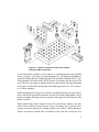
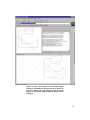
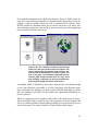
Figure 1.1, below, shows some typical components of an off-the-shelf commercial
modular fixturing toolkit.
1
Alternatively called “fixture synthesis,” “fixturing algorithm,” “automatic fixture configuration generation,”
or “automated fixture design.” These terms are used interchangeably in this thesis.
2
Figure 1.1: Typical commercial off-the-shelf modular
fixturing toolkit components.
In this dissertation I address several aspects of synthesizing and using modular
fixtures. In part 3 I describe my implementation of a 2D fixturing algorithm developed by Randy Brost of Sandia National Labs and Ken Goldberg of USC [[5]].
This algorithm is the heart of the WWW Fixture Server that I describe in part 4. In
part 5 I discuss my design of minimal primitives and efficient fixturing algorithms
in 3D space, and describe an algorithm for modifying part pose in a 3D “constructive” fixture synthesis.
When attempting to develop a new scheme for modular fixturing, one may wish to
know what sort of spatial discretizations are able to facilitate computability. Part 6
analyzes modular fixturing systems in general with regard to discretization of the
fixture variables.
When synthesizing fixture designs for any of several fixture schemes, one may
wish to know which are better in terms of ease of loading. Part 7 presents a discussion of motion planning for loading modular strut fixtures. When planning a
fixture, one needs to consider the accessibility of the work face of the part. It is
3
desirable to order fixture designs on accessibility. Part 8 describes an accessibility
metric for planar facets. Part 9 is a summary and discussion of results and possible
future work.
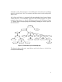
All of the work below is concerned with non-redundant form closure fixtures
without friction. A non-redundant fixture has the minimal number of contact
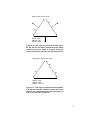
points for form closure, i.e., four for 2D fixtures, and seven for 3D fixtures. Figure
1.2, below, shows a map depicting the relationships among the various topics in
this dissertation:
Modular Fixtures
Taxonomy
of Modular Fixture
Systems
Modular Fixture
Algorithms
2D Fixtures
3D Fixtures
Strut Fixture
System Hardware
Design
2D Fixture
Synthesis
PC
Implementation
FixtureNet
WWW
Implementation
FixtureNet II
Fixed Pose
Resolution-Complete
Synthesis Algorithm
Strut Fixture
Loading
Variable Pose
Greedy Synthesis
Algorithm
Strut Fixture
Accessibility Metric
PC
Implementation
NFS Analysis
Dot Product Heuristic
SFS Histogram
Heuristic
Area Heuristic
FixtureNet III
PC
Implementation
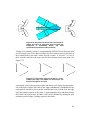
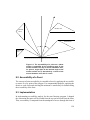
Figure 1.2: Dissertation topic relationship map.
The directed edges in the topic map indicate topical sub-classes or derived-from
or based-on relationships.
4
2. Related Work
In this section I describe work that has been done that is related to my thesis topic
and to work I have performed. I also show how my work relates to that work and
how it fills some gaps in the earlier work.
Much early robotics work focused on an important application of the industrial
robot, mechanical manipulation [[7]]. Research systems such as Marvin Minsky‟s
“Blocks World” (at MIT) integrated robot vision and manipulation. So it is not
surprising that there is a significant body of literature on the topic of grasp planning. Much of the work in this area can be subdivided into categories based on
some obvious questions that occur in attempting to implement a manipulation system:
What constitutes a good grasp?
What part of the object (region set) should be contacted in forming a grasp?
Can the grasp be optimized without undue computational complexity?
Should we consider friction in grasp planning?
How many fingers or contact points should we use?
To simplify the problems and still yield sufficiently general results, many investigators restricted manipulation objects to the set of polyhedra whose boundaries
are sets of polygons [[19]]. Continuing with that tradition, in my work I model
parts as sets of directed polygons (they are contacted only on the outside).
Computer aided design (CAD) forms the heart of a manufacturing information
system. 3D solid models are currently used for product design, and now fixtures
and tooling are being designed with solids (1995) [[20]]. Part modeling is also
essential to algorithms for working with fixtures (synthesis, loading, analysis,
etc.). Manufacturing is concerned with the physical world. Mathematical models
abstract the essential properties of physical manufacturing systems, and computer
representations can be derived from those mathematical models (1980) [[37]], facilitating the development of algorithms. The 2D fixture synthesis algorithm I de-
5
scribe in section 3.1 and the 3D fixture synthesis algorithm I describe in section 5
rely on part modeling as edge sets and facet sets, respectively.
Grasping and fixturing are closely related, though grasp planning tends to be realtime while fixture synthesis is normally done off-line.2 Another distinction is that
modular fixtures generally restrict available part contact points to a finite lattice.
While the geometries of grasping and fixturing are quite similar, the kinematics of
the act of grasping are quite different from the loading of a fixture. In grasping, a
hand or gripper closes around a (usually) stationary object; but in fixture loading,
an already-grasped object is placed into a partially constructed fixture. Then the
remaining pieces of the fixture are built around the part. Questions arise as to the
stability of the part with gravity, in the partially-constructed fixture, and the best
time to remove the grasping hand. Note that grasped interfaces (surfaces) on the
part are not available for contact with the fixture, and that the grasping hand may
interfere with fixture construction. Hence, it is obvious that fixture loading planning is significantly more complicated than grasp planning alone. I build my work
on an extensive body of work on grasping, as well as on smaller bodies of research on fixturing and part feeding.
Flexible manufacturing requires the ability to change factory configurations rapidly as product designs change. As production operation setup costs come down,
batch sizes can be reduced and manufacturers acquire a market agility that yields
an important advantage. In 1987 The Economist produced an extensive survey
titled “The Factory of the Future” (1987) [[8]]. In it, the editors described both
success stories and failures as companies attempt to remain competitive in a rapidly changing world. They emphasized the importance of planning when building
new flexible factories. In particular, my work on strut fixturing relates to factory
automation because a strut fixture can serve as both a pallet and a fixture. A part
can be placed in a strut fixture in a fixturing box assembly. That box assembly can
be passed from robotic work station to station like a pallet. Then when a new fixture orientation is required, the part can be removed from its fixture box and
loaded into a different one, in a new orientation, and the work can proceed at a
new work station. The first fixture box is then returned to fixture another part.
Robotic algorithms (see [[12]] for a comprehensive overview) rely heavily on
computational geometry. See [[34]] for a thorough introductory text. Sedgewick‟s
well known text “Algorithms” [[40]] contains a chapter on computational geometry that I found useful in my various implementations.
2
Fixture synthesis might also be real time in a CAD evaluation loop.
6
2.1 Minimalism Related Work
In “A „RISC‟ Paradigm for Industrial Robotics,” Canny and Goldberg (1993) [[6]]
state the case for returning to fundamentals in robotics research for industry. In an
industrial setting cost and performance are paramount. Anthropomorphism in
computing and mechanisms is inappropriate for most industrial applications, yet
the flexibility that is the hallmark of robotics must be retained. The answer to this
challenge is to use just enough sensing and control to get the job done.
Canny and Goldberg advocate the use of simple sensors, such as binary-state devices like light beam sensors and switches, and the use of simple mechanisms like
parallel jaw grippers. Simplicity in sensing and mechanisms leads to simpler and
faster algorithms, necessary for fast real-time speeds. Assembly tasks for robots
have through-put speed requirements on the order of one cycle per second.
My work on strut fixtures falls into this minimalist RISC paradigm. The fixture
primitives are few in number and except for fixture loading, sensing is not required. Using strut fixtures as both pallets for transporting workpieces to multiple
workstations and as fixtures for holding the workpieces can improve factory
throughput.
Since the appearance of Canny and Goldberg‟s paper, a number of papers citing
the RISC paradigm have appeared, among them, “Object Localization Using
Crossbeam Sensing,” by Wallack and Canny (1994) [[49]], in which the authors
describe the use of an array of binary-state beam sensors for determining the
orientation and location of parts moving on a conveyor belt. While my work does
not deal specifically with object localization, such localization is essential for manipulation of parts prior to fixture loading. I provide an algorithm for fixture loading in section 7.1.1.
A related paper also citing the RISC paradigm is “Sensing Polygonal Poses by Inscription.” (1994) [[16]]. In this paper, Jia and Erdmann describe using revolving
scanning light beam sensors to resolve the pose of prismatic parts by measuring
the inscribed angle from two locations. The described algorithm is very fast, with
a running time that is O(n), and hence quite suitable for an industrial setting. Pose
sensing, a form of localization, is a precondition to fixture loading and for verifying that a workpiece has not slipped during work.
7
2.2 Grasping Related Work
To load a fixture, the part must be grasped by a manipulator. The planning of a
grasp has many similarities to the planning of a fixture. Fixture planning evolved
as a specialization of work in grasping. The statics of grasps and fixtures are the
same, but grasping configurations are oriented toward manipulators and fixture
configurations tend to be based on modular hardware systems.
Mishra et al. (1987) [[23]] had multi-finger dexterous manipulators in mind when
they wrote “On the Existence and Synthesis of Multifinger Positive Grips” in
1987. However, it is a landmark paper for all frictionless grasping and fixturing
work because they proved that seven point contacts are sufficient for any frictionless-graspable3 object. The authors also describe an algorithm for synthesizing
grasps in time that is linear with the number of facets in the object. This algorithm
is generally unsuitable for robotic practice because (1) it is non-optimal and may
generate grasps with many more than seven contacts (redundant frictionless
grasps), and (2) it neglects inaccessible facets such as the region on which the part
rests. Their term “positive grip” is the equivalent of the more modern “form closure.” Both terms denote the positive spanning of the wrench space. This work is
a direct precursor of my own, which leads to the synthesis of non-redundant frictionless grasps. My work also addresses the accessibility of facets (see part 8.2).
The quality of a planned grasp is important to know. Higher quality grasps (and
fixtures) will result in lower grasping forces for a given disturbing wrench set.
Trinkle (1988) [[44]] in “On the Stability and Instantaneous Velocity of Grasped
Frictionless Objects” described a quality metric that is identical to the “generic”
quality metric we used in our strut fixture synthesis implementation (1995) [[45]].
See section 5.3.2 for a discussion of this very useful frictionless fixture quality
metric.
Nguyen (1988) [[26]] works with 2D and 3D objects with and without friction in
“Constructing Force-Closure Grasps.” This paper is an excellent primer on the
subject of form closure and grasping and explains basic concepts very clearly.
Nguyen describes the construction of independent contact regions for form closure
grasps, including direct construction from local regions of constant curvature. One
approach to synthesizing frictionless fixtures for 3D polyhedral parts would be to
compute the independent regions for the facets and then apply a discretization to
3
I adopt the term “FG” (frictionless graspable) for “having the necessary condition for frictionless fixturability” and use it consistently throughout this dissertation (see section 5.6.1).
8
the regions. However, this approach does not solve the problem of which 4, 5, 6,
or 7 facets to use for locating fixels, nor does it reduce computational complexity
in generating complete solutions to the problem of fixture optimization.
A parallel jaw gripper can be used for more than just grasping. By adding an antifriction device to one jaw of the gripper, Ken Goldberg adapted this mechanism
for orienting parts without sensing [[11]]. Loading a polyhedral object into my
strut fixture requires part orienting. The parallel jaw squeeze orientation process
for polygonal parts described by Goldberg can be extended to 3D by using two
grippers and handing off the part, rather than having it rest on a table between
squeezes.
A “pivoting gripper” is a simple extension from a parallel jaw gripper that adds
another degree of freedom about a pivot axis orthogonal to the gripper wrist axis
and parallel to the jaw translation axis. Pivots can be passive or controlled (driven). A passive pivot relies on gravity or some other external force for orienting
the part about the pivot axis and so is in keeping with the RISC philosophy. Rao
and Goldberg (1994) [[35]] describe part orientation with a passive pivoting gripper in “Planning Grasps for a Pivoting Gripper.” The passive pivoting gripper allows the orientation of a part to change about two axes with a single grasp and
placement. The grasp of the part must not only be stable when the jaws close on
the part, but should lead to an orientation that is stable in the desired pose when
the part is put down. In strut fixture loading, the part is placed in contact with
three or four struts, and must be stable with friction under the force of gravity
when it is released from the gripper.
Although computation is often simplified by neglecting friction, it is generally
present to some extent. Rao and Goldberg (1994) [[36]] show that any planar part
with deterministic friction has an equivalent dual part without friction in “Friction
and Part Curvature in Parallel-Jaw Grasping” and, extending previous results, derive grasp plans for parallel jaw grippers with friction. These plans could find application in an implementation of my fixture loading algorithm in section 7.1, below.
Recently Jean Ponce4 has taken a new direction in grasping that has some important implications for fixturing. Ponce et al. (1995) [[31]], in “Computing the Immobilizing Three-Finger Grasps of Planar Objects,” describe applying the concept
4
University of Illinois, Urbana. Jean Ponce visited USC in the summer of 1995 and delivered some lectures
on the subjects of grasping and modular fixtures. Urbana Illinois is also the birthplace of the fictional HAL
9000 computer, 1995 (2001, a Space Odyssey, screenplay by Arthur C. Clarke, directed by Stanley Kubrick).
9
of “immobilizing grasps” to frictionless polynomial planar objects. With frictionless objects, these “grasps” are much like cams, kinematically designed to force
grasping fingers apart; but with friction, which is always present, these grips could
be useful. For the obvious extension to 3D, Ponce et al. (1995) [[33]] utilize friction in three dimensions in “On Computing Four-Finger Equilibrium and ForceClosure Grasps of Polyhedral Objects” and (Ponce et al. (1995) [[32]]) “Algorithms for Computing Force-Closure Grasps of Polyhedral Objects.” The four finger grasps utilize what Nguyen (1988) [[26]] called “force-direction” closure5, a
previously under-rated aspect of grasping and fixturing. These four-finger frictional grasps have an enormous potential for application in light-duty fixtures.
Ponce also describes a highly efficient algorithm suitable for real-time computation of these grasps [[30]].
In computing grasps (or fixtures) it is useful to have some metric of the quality of
the grasp. Bud Mishra gives a detailed treatment of this subject in “Grasp Metrics” [[22]]. There are two related algorithmic problems: the computation problem (“computing the quality of a given grasp under the chosen grasp metric”) and
the optimization problem (“computing the optimal grasp of an m-fingered hand
under the chosen grasp metric”). Solutions to these problems find use in both my
2D and 3D fixture synthesis applications. For my 3D fixturing program, I use
what I call a “generic” quality metric. This metric was suggested by Jeff Trinkle
[[43]] and is called “rnull” by Mishra.
2.3 Fixturing Related Work
There is a significant body of literature on the subject of fixturing, including an
engineering handbook published by the Society of Manufacturing Engineers
(1989) [[3]].
2.3.1 Friction
Static analysis can take friction into account or it can neglect friction. Neglecting
friction simplifies analysis: where friction plays a role, analysis is problematic. It
is an accepted engineering practice never to rely on friction in structural design
and, where friction is undesirable, such as in many mechanisms, there always
seems to be too much of it. Structural strength analyses generally neglect friction
for conservatism. If a structure will survive without friction it will certainly maintain integrity with friction. Because fixtures are often used where large dynamic
5
The force direction space is closed if the set of direction vectors positively span the space.
10
forces might be imposed such as in machining, frictionless analysis is the rule in
fixture design. However, due to recent work by Ponce et al. [[33]] in the field of
grasping, fixtures utilizing friction may begin to be seen more frequently in assembly or other operations where anticipated loads are light. A four-fingered
grasp with friction of a polyhedral object can provide a good model for a lightduty fixture for assembly.
For my strut fixtures, I assume there is no friction for the computation of form
closure. The struts are normal to their contacting faces so there is no tangential
component of load for a perfectly aligned strut. In reality, however, no strut is perfectly aligned, so some small amount of friction is necessary (and will be present)
to keep the strut from slipping as the fixture is assembled, or the part is disturbed
in its fixture by loads induced by assembly or other operations.
2.3.2 Form Closure
A form closure grasp is also called a “positive grip” [[22]]. These grips can be either with friction or assumed frictionless. Force/torque closure is equivalent to
form closure [[22]].
Reuleaux (1876) [[38]] in “The Kinematics of Machinery” first described form
closure which captures the intuitive requirement of a fixture: a part is held in form
closure if it can resist arbitrary forces and torques. Lakshminarayana (1978) [[17]]
showed that seven frictionless contacts are necessary to hold a 3D part in form
closure; Mishra (1987) [[23]] showed that seven frictionless contacts are also sufficient. My strut fixtures algorithm (section 5.3) is designed around this sevenpoint frictionless contact necessary and sufficient condition for form closure.
Goldman and Tucker (1956) [[13]], in a purely mathematical paper on linear algebra, described the necessary and sufficient conditions for positively spanning an ndimensional Euclidean space, which coincidentally describes the necessary and
sufficient conditions for form (force/torque) closure.6 Their theorem helps to provide a proof that my form closure test is valid.
Various publications differ in their application of terminology to the various grasp
conditions. I use the term “form closure” to mean fixture contacts rigidly held to
generate reaction forces at the contact positions (wrenches) that, taken together
with any disturbing wrench set, close both the force space ( 3) and moment space
6
Force/torque closure and form closure are equivalent. See [[23]], section 2.5, page 144.
11
( 3). Consistency in terminology is desirable, but a standard terminology has not
yet emerged in the robotics literature. “On Force and Form Closure for Multiple
Finger Grasps” by Rimon and Burdick (1996) [[39]] seeks to remedy the situation
by precisely defining several terms, including “force closure,” “form closure,” and
“immobilizing grasp.” While their definitions are no doubt correct, the terminology still leaves some confusion in place. For example, they offer the alternative
term “wrench closure” for “force closure.” Rimon and Burdick‟s “force closure”
is what Mishra [[23]] calls “force/torque closure” (for which I prefer the term
“force/moment” closure because it is more consistent with mechanical engineering practice7). “Force closure” is used in several other publications to indicate the
closure of the force direction space, and that is the meaning I prefer for the term.
2.3.3 Modular Fixturing
Asada and By (1985) [[2]] in “Kinematic Analysis of Workpart Fixturing for
Flexible Assembly with Automatically Reconfigurable Fixtures” describe an automatic fixture reconfiguration system using a robot manipulator and a CAD system to provide a systematic method for designing fixtures. They also provide an
analytic test for form closure and suggest how contact points might be applied, but
they do not consider how a restricted set of modular elements could be used to
reach those points. They call fixture synthesis “designing a fixture layout,” which
is in keeping with the mechanical drawing practice of calling a drawing that gives
the locations of parts a “layout” drawing. They develop analytic tools for designing fixture layouts using a set of hardware primitives implemented at MIT. They
also consider loading and unloading of their fixtures. However, they provide no
algorithm for the synthesis of fixture configurations.
Hoffman‟s text (1987) [[14]] provides an overview of conventional practice with
modular fixtures. For example, machinists are taught the 3-2-1 rule of fixture design: The part is first set on top of three locators (tooling balls, for example), then
it is slid so that one edge is in contact with two locators, and then it is slid in contact with those five locators so that it contacts the final locator. Then at least three
clamps are applied to secure the workpiece. This method works well for many
7
“Moment” means a pure couple regardless of its orientation. “Torque” means a moment aligned with a particular axis. For example, a drive shaft is designed to transmit torque. When in operation, a drive shaft can
experience transverse moments due to inertial loads. The moment load in the drive axial direction is the torque that is transmitted. In beams, engineers speak of “bending moments” (transverse moments) and “torsion”
(axial moment).
12
parts (especially prismatic solids), but the part is overconstrained8 with nine contacts, and having more faces available for work (as with my 7-strut fixtures) will
require fewer setup changes.
In ranking fixtures, several quality metrics can be used. For fixture synthesis algorithms that output one or more dimensions of part pose, the accessibility of the
part in its generated pose can be a factor. Spyridi and Requicha present an analysis
of accessibility of polyhedral parts in “Accessibility Analysis for the Automatic
Inspection of Mechanical Parts by Coordinate Measuring Machines” (1989)
[[41]]. In “Accessibility Analysis for Polyhedral Objects,” Spyridi and Requicha
provide an algorithm for computing global accessibility cones (GACs) and show
the results of their implementation. For the purpose of ranking the accessibility of
a given facet in the strut fixturing box, I found a computationally simpler approach that preserves the accessibility order of various part poses without quantifying the accessibility for a specific purpose.
Wolter and Trinkle (1994) [[53]] describe a non-modular fixture synthesis that
uses analysis of frictionless stability in “Automatic Selection of Fixture Points for
Frictionless Assemblies.” This is an impressive paper because it applies to both
2D and 3D fixtures, but it is “non-modular” because the fixture points selected are
from a continuum in space and not from a discrete set of locations. In this problem, frictionless elements of assemblies need to be held together by a fixture.
They analyze fixtures for “stability” in terms of virtual work. Their fixture synthesis algorithm uses a “shotgun” approach: they scatter fixels about the assembly
and solve a linear program to minimize contact forces at the fixels by having fixel
location on the part boundary be a system variable. Fixels that have reaction
forces of zero get discarded. This is an effective approach, but it is not guaranteed
to find an optimal solution, and it is not applicable to modular fixturing hardware
sets as currently available. Their approach can be considered “complete” if it can
be guaranteed to find a solution when one exists or to report failure when one
does not exist. The authors do not discuss completeness as such, but from examining their mathematics, I conclude that their algorithm is complete.
Brost and Goldberg (1994) [[3]] have demonstrated a complete algorithm for synthesizing 2D fixtures that forms the basis of my FixtureNet (part 4) implementation. The Brost-Goldberg algorithm is described in more detail in part 3.1. Since
that paper was published, other papers regarding planar modular fixturing have
8
Statically indeterminate. Computing reactions for statically indeterminate systems requires knowledge of
the stiffnesses of all the interfaces.
13
appeared, including “Planning for Modular and Hybrid Fixtures” by Wallack and
Canny (1994) [[49]], which describes a vise-like fixture with four cylindrical locators. Clamping motion is provided by a translating lattice, and a complete algorithm evaluates all possible configurations: First they enumerate all jaw-specified
edge segment quartets. Then for each quartet they enumerate all combinations of
jaw contacts. Next they compute the peg configurations that simultaneously contact the quartet. Finally, they compute the contact points and test for form closure.
Their algorithm has a higher computational complexity than that of BrostGoldberg because it considers all quartets of edges rather than triples.
An interesting topic is the existence of modular fixtures. Given a particular part, if
no modular fixture can be found for it, given a modular fixturing system, we can
say that the part is “not fixturable” within the given system. This fixturability
question is important because, if we can determine the existence (or more importantly, the non-existence) of fixtures easily, we can avoid futile computation. Y.
Zhuang, K. Goldberg, and Y. C. Wong explored this issue for planar parts in a
grid locator system in “On the Existence of Modular Fixtures,” [[55]] and identified a class of parts for which no fixtures with three locators on a grid exist. In my
work, I developed a “fixturability test” for 3D parts modeled as sets of directed
facets. This class of parts includes all polyhedra. This fixturability test serves as
an important tool in my algorithms in identifying the necessary and sufficient subsets for fixturability of a part.9
Recently, Ponce described “immobilizing” grasps (1995) [[31]], and proposed
their possible application in fixturing in both two and three dimensions. Immobilizing fixtures require only three contact points in the plane and four contacts in
three dimensions. Ponce says “a sufficient condition for immobility is that the relative curvature form associated with an essential equilibrium grasp or fixture and
defined by
d
k rel
i
wi k i
i 1
be negative definite.” The weights i are the equilibrium weights of the contact
wrenches and |wi| is the magnitude of the wrench exerted by locator i. The practical application of immobilizing fixtures is quite limited, however, in that when
9
My fixturability test determines the existence of any frictionless grasp for a set of directed facets, without
regard to fixturing hardware or manipulator configuration. The existence theorem of [[55]] is with regard to a
particular fixture hardware set.
14
they are evaluated in terms of the quality metrics generally applied to form closure
fixtures, they will be ranked below fixtures with form closure.10
The Brost-Goldberg algorithm for 2D fixture synthesis (and any similar algorithm
such as that of Wallack in [[49]], above) applies to parts modeled as directed edge
sets. This class of parts includes polygons. Some authors refer to a polygon as a
2D polyhedron, which is fair enough, but tends to add to the occasionally confusing terminology in fixture work. Extending such an algorithm to also apply to
more generalized edges will increase the range of its utility. One such generalization of straight edges is to include circular arcs. Aaron Wallack and John Canny
do exactly that in “Modular Fixture Design for Generalized Polyhedra” (1996)
[[50]]. I have proposed an approach to the same problem in section 9.3.1.
Aaron Wallack describes a generic approach to modular fixture synthesis algorithms in “Generic Fixture Design Algorithms for Minimal Modular Fixture
Toolkits” [[47]]. He bases his approach on an observed duality between modular
fixture synthesis and index sensing. He assumes a “minimal”11 modular toolkit
but concentrates only on systems with one degree of continuity in the fixel set. I
describe a fixture system categorization scheme that covers the full range of minimal modular frictionless form closure fixtures in part 6.
2.3.3.1 WWW Fixture Service Related Work
The Internet offers tremendous potential for rapid development of mechanical
products to meet global competition. In 1995, Ken Goldberg, Giuseppe Castanotto, and I (with assistance from Steve Gentner, Jeff Wiegley, and Mourad Zerroug)
implemented a World Wide Web (WWW) fixture synthesis service based on an
algorithm by Randy Brost and Ken Goldberg [[5]]. The FixtureNet universal resource locator (URL) is:
http://teamster.usc.edu/fixture
Earlier, under Ken Goldberg‟s direction, the USC Institute for Robotics and Intelligent Systems (IRIS) Modular Robotics Laboratory had created the landmark robotic Web sites Mercury Project and The Tele-Garden [[21]].
10
One useful fixture quality metric evaluates fixtures in terms of their ability to react loads applied to the
fixtured part. For rigid parts, immobilizing fixtures generate large reactions for moment loads. Quality metrics are discussed in more detail in part 3.2.3 and in Bud Mishra‟s “Grasp Metrics” [[23]].
11
Aaron uses the term “minimal” here to have the same meaning as my use of “non-redundant”: the minimal
contact set for form closure has no redundant fixels.
15
Related Web sites include the following. All of these can be reached from our
FixtureNet “Related Links” page:
Raju Mattikalli and Pradeep Khosla's online fixturing system at Carnegie
Mellon University. It performs analysis of a given set of 3D wrenches (to
determine if they provide form closure).
http://www.cs.cmu.edu:80/afs/cs.cmu.edu/user/rajum/www/fix4.html
University of Minnesota's Geometry Center has a great collection of interactive geometric algorithms.
http://www.geom.umn.edu:80/apps/
David Eppstein's Discrete and Computational Geometry page.
http://www.ics.uci.edu/~eppstein/geom.html
Jeff Erickson has been maintaining a small collection of computational
geometry World Wide Web pages.
http://www.cs.berkeley.edu/~jeffe/compgeom.html
Prof. Antonio Bicchi's Non-Holonomic Motion Planning Site at University
of Pisa allows users to define obstacles for path planning and even sets up
a standard for others to submit algorithms for comparison.
http://www.piaggio.ccii.unipi.it/prova/motion.html
The AutomationNET!, in December 1995 PC Computing was one of the
best engineering Web sites.
http://www.AutomationNET.com/
FixtureNet was preceded by The Mercury Project (no longer exists) and the TeleGarden (http://telegarden.aec.at/) Web projects. These two projects allowed users
all over the world to teleoperate robots and obtain image feedback. The TeleGarden was also an experiment in virtual community [[21]].
2.4 Fixture Loading Related Work
Ken Goldberg, in “Completeness in Robot Motion Planning” (1994) [[10]], defines exact and complete algorithms and originates the idea of the “solution completeness” of planning problems. An “exact” algorithm is one that is guaranteed to
find a solution if one exists. A “complete” algorithm is exact and will report fail16
ure if a solution does not exist. A problem class is “solution complete” if a solution exists for all instances of a problem. Yan Zhuang et al. showed that a certain
class of 2D modular fixturing problems was not solution complete in “On the Existence of Modular Fixtures” (1994) [[55]].
Fixture loading can be regarded as a type of assembly operation. The automatic
generation of assembly plans and the characterization of the complexity of assemblies are now possible due to the notion of non-directional blocking graphs
(NDBGs) introduced by Wilson and Latombe (1995) [[52]] in “Geometric Reasoning about Mechanical Assembly.” They showed that NDBGs can be computed
in polynomial time and they implemented planning algorithms for use with the
Robot World system. In addition, they defined multiple dimensions of assembly
complexity for evaluating product designs.
Like all robotic operations in the physical world, fixture loading is subject to uncertainties. Sets of points in physical workspaces are referred to as “natural sets”
by Randy Brost in “Natural Sets in Manipulation Tasks” [[4]]. Natural set-based
models support “powerful, general-purpose analysis techniques,” including backprojection.
2.4.1 Fixture Loading Planning
Yu and Goldberg (1995) [[54]] describe loading a “smart” planar fixture in
“Loading Planar Fixtures in the Presence of Uncertainty.” The smart fixture has
electrically sensitive cylindrical locators that report the contact state with a metallic flat part. The planning algorithm switches modes depending on the state of the
locator contacts and generates plans for fixture loading with a switchedcompliance pusher.
Penev and Requicha (1995) [[29]] show how 2D fixtures can be “foolproofed”
with extra cylindrical elements to prevent parts from being loaded in the wrong
pose in “Fixture Foolproofing for Polygonal Parts.” Their algorithm generates optimal foolproofing plans for a given planar fixture. My proposed work focuses on
3D fixtures. It is conceivable that foolproofing might have some advantages for
3D fixtures. However, if one assumes that fixture loading is performed by robots
not using trial-and-error algorithms, the advantages of foolproofing will be minimal.
Arbib and Liaw (1995) [[1]] apply a hierarchical system of sensorimotor “schemas” to the understanding of frog behavior and show how this schema theory can
be applied to robotic problems. This schema theory does not seem to be funda17
mentally different from the hierarchical paradigm espoused in Marvin Minsky‟s
popular book Society of Mind. Fixture loading (see section 9.2.3) and other part
hand-off planning can likely benefit from these and similar system-level distributed approaches. For example, RISC style sensors can be added to strut fixtures
(defined in section 5, below) by putting a contact switch at the end of each strut.
The contact state of each strut will then be known by the robot during the loading
process. Likewise, the part grasping manipulator can be similarly instrumented.
Such a configuration lends itself to the application of sensorimotor schema.
18
3. Modular Fixturing in the Plane
Commercially available modular fixturing hardware sets are well suited for constructing planar fixtures. A planar fixture prevents planar motion: translation and
rotation. While 3D parts with one flat surface can often be fixtured using planar
analysis, parts that are suited for planar fixturing are often flat in nature, perhaps a
short prismatic extrusion of a polygon. Other parts suitable for planar fixturing
might not be flat overall, but will have some planar surface for interfacing the fixture platen, and will be fixtured for some operation that imposes only light forces,
such as assembly, so that vertical cylindrical posts and a side clamp will provide
sufficient restraint.
In practical use, a planar fixture also restrains out-of-plane motion (because of
friction), but the flat nature of the part to be fixtured makes the relevant fixture
synthesis considerations planar, while out-of-plane motion can be restrained by a
top clamp.
3.1 The Brost-Goldberg Algorithm
As mentioned in section 2.3, in “A Complete Algorithm for Designing Modular
Fixtures for Polygonal Parts,” [[5]] Randy Brost and Ken Goldberg described the
first complete algorithm for synthesizing fixtures for a commercially available fixture set. Because it is complete, the Brost-Goldberg (BG) algorithm is guaranteed
to find the optimal fixture by ranking the solutions on a quality metric. The BG
algorithm assumes frictionless contacts. The frictionless assumption is conservative and considerably simplifies computation. The BG algorithm determines form
closure by mapping reaction forces onto a “force sphere,”12 and then constructing
the set of form-closure clamp placements from patches on the sphere that span the
force space. These patches are mapped back to the part, and discrete clamp locations that fall within those mapped edge segments are possible clamp placements.
The BG algorithm was first implemented by Randy Brost on a Unix-based Lisp
machine with X-window graphics libraries. Randy told me that he was not particularly concerned about performance or memory efficiency because of the effectively unlimited virtual memory supplied by the Unix operating system.
12
The force sphere is called a “wrench map” by Mishra in [[22]].
19
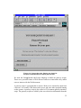
3.2 Personal Computer Implementation
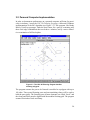
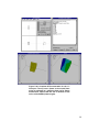
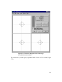
In order to demonstrate performance on a personal computer sufficient for practicality in industry, I wrote the USC 2D Fixturing Program, a Microsoft Windows
implementation of the BG algorithm (see Figure 3.1). This program, like Randy
Brost‟s Unix/Lisp prototype, finds the best fixture for a part by examining only
those fixel-edge combinations that can lead to a solution, not by a naive exhaustive examination of all fixel triplets.
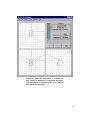
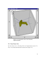
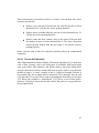
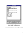
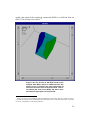
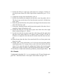
Figure 3.1: The USC 2D Fixturing Program handles
arbitrary polygons.
The program assumes the part to be fixtured is modeled as a polygon with up to
100 sides. Three round fixturing posts and one translating clamp will be used to
hold the part rigidly. The fixturing posts (fixture elements) are called “fixels” and
the clamp and fixels must be aligned with the modular fixturing grid. The program
assumes frictionless fixels and clamp.
20
Implementing the BG algorithm on a personal computer (PC) imposes some
memory limitations. I wanted to demonstrate performance such that my implementation would be practical in an industrial setting. A technician or engineer user would probably not be happy waiting days for a solution set to a fixturing problem.
The industry standard PC today is based on the Intel x86 processor. A typical system has an 80486 or a Pentium CPU (includes on-chip FPU) with 66 to 120 MHz
internal clock speed and 8 to 30 MB RAM, running Microsoft (MS) Windows
version 3.1. MS Windows running in “enhanced” mode (typical of industry practice) transparently provides up to 64 MB of memory by using virtual memory
when RAM is full. A typical system will use 2MB of RAM for disk caching as
well.
The BG algorithm uses cylindrical locators (fixels) on an alternating grid. These
locators are shrunk to a point by “growing” the part by the fixel radius. This is accomplished by moving the edges outward by the fixel radius. Edges that are part
of a concavity in the part will trim each other. “Stay-out” zones are a feature of the
BG algorithm that I implemented as well. Parts can be input with a part drawing
tool (which saves a part file). Stay-out zones can be added or deleted using the
part drawing tool as well.
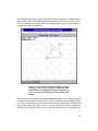
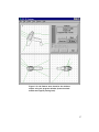
21
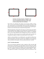
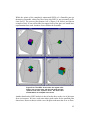
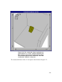
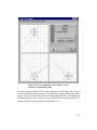
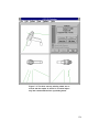
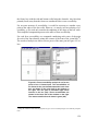
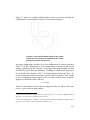
Figure 3.2: The “Aluminum Bracket” is shown in the
part drawing tool. The stay-out zone is shown in red.
The user accesses the part drawing tool from the "Tools" menu. Parts can be
drawn with the mouse. Instructions for using the part drawing tool are shown in
the text area near the bottom of the window. Polygonal part and stay-out zone vertices are drawn in counterclockwise direction. Polygons are limited to 100 vertices. Parts are drawn with black lines and stay-out zones are shown in red. One can
add up to 100 stay-out zones of up to 20 vertices each. When the stay-out zones
are grown later by the program, their convex hull is taken first. If one needs concave stay-out zones, he or she can draw them as collections of convex stay-out
zones.
As the user draws by clicking the mouse on the desired vertices, the current X and
Y coordinates are shown in the text area just below the menu bar. The X and Y
axes coincide with the bottom and left borders of the drawing window, respectively. The desired snap granularity is set in the "Options" menu. One uses the "Edit"
menu to add and delete stay-out zones. Completion of the part and each stay-out
zone is performed by clicking the mouse on top of the first vertex. If one changes
22
the snap setting during drawing, he or she should make sure it is compatible with
the first vertex coordinates.
The user can name the part from the "Edit" menu. When the part is saved, the
program automatically shifts it in X and Y so that the part and its stay-out zones
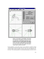
will have a 10 unit clearance from the X and Y axes.
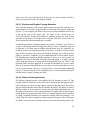
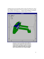
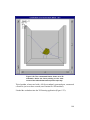
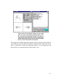
Figure 3.3: During fixture computation, the part is
grown by the fixel radius. The stay-out zone is also
grown. Notice how the stay-out zone incorporates
the curve of the fixel. This is necessary should a
grown part edge intersect a corner of the stay-out
zone.
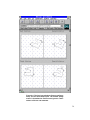
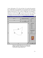
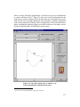
23
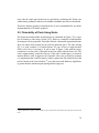
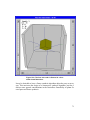
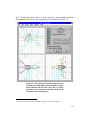
Figure 3.4: The completed fixture set has 151 elements. The best fixture has a quality metric of 1.0
and all the rest have lower rankings. This particular
metric prefers fixtures that resist both in-plane
forces in all directions and in-plane torques in both
directions.
3.2.1 Part Transformation
Once three candidate locators (discrete fixels) are found, there are up to two possible poses for the part in contact with them. The part is transformed into the fixture workspace and the possible clamps for each of the two poses (many cases
have but one pose possible) are enumerated and tested for form closure. The transformation of the part was a bit tricky. I at first wrote an iterative procedure that
24
worked well in most cases but for which I had difficulty demonstrating correctness. Xiaofei Huang (see part 10) came to the rescue with an analytic transform
that he adapted from Horaud [[15]]. This analytic transform contributes to the relatively good performance of my implementation.13
3.2.2 Fast Test for Form Closure
I had some difficulty implementing the BG force sphere mapping described in the
paper [[5]]. Brost and Goldberg had mapped the fixed locator contacts to the
“force sphere” (wrench space) and constructed regions in which the positive spanning of this space would result. These regions were then mapped back to the part
to define edge intervals wherein clamp placement would result in form closure.
Thinking about what constitutes a fixture, I invented my own analytic form closure test, which in my opinion is the simplest and fastest theoretically possible. I
called it the “fast form closure test.” I did not know at the time that equivalent
tests had recently been popping up in the literature. Later, for my 3D program,
Yan Zhuang (see part 10) helped me formalize a proof of my form closure test,
and found that an equivalent mathematical proof was published in 1952 by Goldman [[13]]. Yan was able to find a simplification of the Goldman proof, and that
is what appears in our paper on 3D strut fixtures [[45]]. For more details on the
“fast form closure test” see section 5.3.1.
Bypassing the mapping of force sphere regions to the part edges and instead applying possible clamps and testing them for form closure contributed to the good
performance of my implementation.
3.2.3 Quality Metrics
Each time a new fixture set is calculated or an old one is loaded, it is sorted and
displayed according to the default quality metric. The default quality metric minimizes the fixel reaction forces when a unit clamping force is applied. Other
quality metrics are available from the "Options" menu. The "Resist Force" metric
minimizes reactions at the four fixture points for general forces applied to the part
at the average of the reaction points. The "Resist Torque" metric minimizes reactions for both clockwise and counterclockwise torques. Various combinations of
these force and torque metrics are also available (25/75, 50/50, and 75/25). For
general use, either the default or the 50/50 quality metrics are recommended.
13
On a Pentium machine all test runs completed within a few minutes, including a 30-gon part.
25
Figure 3.5: The quality metric options are accessed
via pull-down menus.
Choosing the "Custom..." quality metric option displays a dialog box that allows
the user to enter a combination of X and Y forces and Torque (Mz). Checking the
"Absolute" check box applies the force in the fixture grid reference frame, rather
than relative to the part‟s reference frame. The force is applied to a point on the
part that is the average of the fixture points, and reactions are calculated.
26
Figure 3.6: The custom quality metric dialog window.
To the uninitiated it might appear that such a calculation is statically indeterminate and cannot be done without knowledge of part and fixture compliances. Were
that the case, quality metrics would indeed be much more difficult to compute.
Note, however, that when a force is applied to a four-contact fixture, only three of
them generate positive reactions. The calculation is done for the combinations of
three contacts. The set that produces all positive reactions is valid and the maximum reaction is used as the quality metric. The fixture with the minimum maximum reaction is best.
27
4. FixtureNet
4.1 Summary
Together with Ken Goldberg, Giuseppe Castanotto (see part 10) and I have implemented a WWW server to provide modular fixture design alternatives to engineering users around the world. I refer to our server system as FixtureNet. Giuseppe worked on the Web interface and I worked on the fixture synthesis server.
Manufacturing engineers build modular fixtures from a small set of reusable parts.
We based our FixtureNet on the Brost-Goldberg algorithm [[5]], which takes a
polygonal part description as input and generates form closure fixtures using three
locators and one clamp mounted on a regular lattice of holes. FixtureNet returns a
set of solutions, sorted by quality metric, along with images showing the part as
the fixture will hold it in form closure for each solution.
This implementation handles fixture design for flat polygonal shaped parts in the
size range of four inches in diameter up to any size that the fixture platen will accommodate—generally about 20 inches, for the commonly used fixture sets.
4.2 Web Access
Users can gain access to this service with the Netscape WWW browser, and can
send part specifications to the server in several ways. The user can enter the coordinates of the part vertices manually through the keyboard, prepare a file listing of
the coordinates which the server can read, or submit an image of the part. In the
latter case, FixtureNet uses an image-recognition program to extract the edges and
vertices of the part automatically.14
4.3 Algorithm
Because it is based on the Brost-Goldberg algorithm (section 3.1), the FixtureNet
algorithm is complete in the sense that it will find all solutions that exist for a given fixture platen grid pitch and will return failure if no solution exists. FixtureNet
then sorts the solutions by a quality metric.
14
This image recognition feature of FixtureNet is still vaporware as of this writing.
28
The default quality metric prefers parts that are most resistant to a combination of
forces in the plane of the fixture and moments about a normal to the lattice plane.
Users can specify other quality metrics, including preference for fixtures that resist particular load combinations.
Figure 4.1: The USC 2D fixturing program is shown
running in slave mode as part of FixtureNet. Note
that the menus are grayed out and not accessible to
a user. The request ID being serviced is shown at the
bottom.
When FixtureNet finishes the solution computation (under a few minutes for most
parts), the server notifies the client, and FixtureNet displays the first (highest quality) fixture for him along with a listing of the locations of the fixture elements and
the position of the part in the fixture. FixtureNet tells the user how many fixture
solutions it has found, and the user may step through them all, examining an im-
29
age of each, in order of the quality metric. Output images from the FixtureNet are
similar to Figure 3.4 shown above.
4.4 Architecture
The FixtureNet system architecture is shown in Figure 4.2. The client service requester submits the part description via the Internet. The Unix HTML server assigns a service request number (unique identifier) and contacts the fixture server
program running on a separate machine in a Microsoft Windows environment.
FixtureNet, in turn, spawns a new process to do the fixture computation for the
particular service request. In this way, FixtureNet can handle multiple requests
simultaneously by spawning a new Windows fixture process for each service request from the Unix server.
Unix
Host: teamster
MS Windows
Host: teaser
HTML Script
Fixture Synthesizer
DDE
HTTP Server
Fixture Server
Pentium
486
Socket Connection
to Internet
Ethernet LAN
Figure 4.2: FixtureNet system architecture.
FixtureNet is a prototype for a useful engineering service. The user-friendly interface and the cross-platform support of Netscape will allow the widest possible
access for this state-of-the-art fixture design service.
The USC FixtureNet service is currently accessible via the following uniform resource locator (URL):
30
http://teamster.usc.edu/home/fixture/
The user accesses the Teamster HTTP server (a Linux client with respect to the
fixture server on Teaser) via the Internet (with Netscape or some other WWW
browser application). The ability of the user to describe the part to be fixtured by
drawing with the mouse is a convenient feature15. The mechanism behind image
maps is straightforward: the image that we wish to use (in our case a square where
the user can draw his or her part) consists of an array of picture elements (pixels),
and the coordinates that define these points are determined by the local operating
system and recorded by the browser application when the user clicks his or her
mouse. When the user selects a point, its coordinates are passed to a drawing program (written in the C language). The coordinates are stored for use when the part
will be submitted to FixtureNet. The user can also enter the part vertex coordinates manually through the keyboard, prepare and send (by FTP) a file listing of
the coordinates which the server can read, or change and submit default input16
provided in input text boxes.
15
But for serious use with real parts we emphasize that the user can submit a descriptive file via FTP.
16
Several simple sample parts, including a square, a pentagon, and a star, are provided for those desiring a
quick trial of FixtureNet.
31
Figure 4.3: If more than zero fixtures are found for
the part, FixtureNet offers to display the best four.
We used the Unix Bourne shell script language to build our gateway scripts.
These are a powerful feature of Web browser and server interaction: they enable
users to interact with the Web document.
A gateway script is a program that is run on a Web server activated by input from
a browser. It is usually a link between the server and some other program running
on the system. A gateway script is also called a CGI (common gateway interface)
script. The gateway scripts are called by the server based on information from the
32
browser. The URL points to a gateway script in the same way that it points to any
other HTML page on a server; when the server receives the request, it notes that
the URL points to a script (based on the file location, usually the cgi-bin directory) and executes that script.
The script performs some action based on the input, in our case, simply to call a
correspondent C program. After this the script formats its result in a manner that
the Web server can understand. The Web Server receives the result from the script
and passes it back to the browser, which formats and displays it for the user. FixtureNet uses 13 different gateway scripts and 13 correspondent C programs. Each
script is a Web server interface to call a C program binary.
33
Figure 4.4: The four best solutions (fixture configurations) for the hook-shaped part. The default quality
metric is formulated to resist several generic combinations of forces and moments.
34
When the part is submitted, FixtureNet parses the input in accordance with the
input format specification (described for the user on the “explanation” page). If an
error is found, a message is returned to the user. Otherwise, FixtureNet opens
network communication with the fixture server on machine A (Teaser) and sends
the formatted input part.
After the Linux client sends the fixture server the data describing a polygonal part,
the fixture server initiates the fixture design algorithm by spawning a fixture synthesis process which estimates run time based on part size and grid pitch.17 The
estimate is returned to the Linux client, which formats it into an HTML page and
returns it to the user.
When the fixture synthesis program completes the design algorithm, it communicates the data via Windows dynamic data exchange (DDE) to the fixture server,
which relays it to the Linux client in the form of textual descriptions of solutions.
Each solution includes the pose (position and orientation in the plane) of the user's
part, the position of three locators on the lattice, and the position and offset for a
clamp such that the part is held in form closure.
The Linux client then runs a custom graphics routine to generate (CompuServe‟s)
graphic interchange format (.gif) images of the part in each of the best four solutions.
Communication via Berkeley sockets is the key to building a cross-platform
WWW service of this kind. We used the Windows Socket application programming interface (API), a subset of Berkeley sockets. For rapid development we implemented the algorithm in Visual Basic using a Windows Socket custom control
(a precompiled MS Windows dynamic link library (DLL)) from Distinct Corporation.
A number of architectures can be used for communication with sockets. We experimented with several before finally settling on using a single client socket in the
Linux client and a server socket in the fixture server. We used a 7-bit ASCII string
to pass information through the socket connection formatted with an 8-digit service request identifier and a 3-digit type code.
17
The grid pitch is the inverse of the distance between holes in the fixture plate. For example, a plate with
holes spaced two inches apart has a grid pitch of one half (holes per inch), while if there were one half inch
between holes, the pitch would be two. The hardware has a maximum grid pitch, but by ignoring every other
hole, we can reduce the virtual grid pitch by half, reducing computational complexity.
35
The Linux client initiates a fixture service request with a socket connect request
and an initial fixture request message (code 001) that includes the part data (number of vertices and x-y coordinates of each vertex) and the desired grid pitch
(coarse, medium, or fine). When the fixture server receives the request, it responds with a “request acknowledged” string and then spawns an instance of the
fixture synthesis program which, in turn, generates a time estimate for the job
based on the current CPU load and the part parameters. When the Linux client
requests job status, the fixture server then relays the fixture synthesis program
time estimate and state to the client. While multiple fixture synthesis program instances can be run simultaneously, the throughput of the system will not be increased by doing so. FixtureNet can be easily extended by adding additional server machines.
4.5 Usage Statistics
FixtureNet was first operational and publicly available in July of 1995. Some
problems were identified at that time and remedied in August. Incremental improvements were incorporated through November, and usage statistics were compiled starting December 16, 1995. FixtureNet has been publicly available continuously since then. From December 16, 1995, to March 31, 1996, the FixtureNet
usage statistics are:
FixtureNet Statistics
Number
Requests of FixtureNet service input (keyboard):
66
Requests of FixtureNet service input (drawing):
111
Solution sets delivered:
142
Total fixture configurations computed:
8732
Table 4.1: FixtureNet Statistics
In many cases (35, 25%), users jump to another page and do not return to request
to view the solutions. These solutions are computed, but are not delivered or captured into the “sets delivered” statistics. A typical run time for a fixture computation is about a minute. The “square” example part takes four seconds.
36
4.6 FixtureNet II
Charles Anderson of Berkeley created a Java interface to replace the CGI system
of FixtureNet. This allows a more natural feeling user interface and adds greater
display capability. For example, Charles added reaction visualization to the fixture
display. The user clicks on a point on the part and drags with his mouse. The distance dragged represents a force vector, and the reaction vectors for the fixture are
displayed visually.
The fixture server and synthesis program were run on a Pentium and gave good
performance, but there were still some communication problems that resulted in
occasional down-time, which motivated the all-Java FixtureNet III, below.
4.7 FixtureNet III
I ported the essence of the fixture synthesis program to Java as an applet (Sun‟s
name for a small Java application intended to be run in an applet viewer, such as
Netscape 3.0 or better).
This applet is shown in Figure 4.5 and Figure 4.6, below.
37
Figure 4.5 The part is drawn in the smaller upper
window in FixtureNet III. Stay-out zones are shown in
red. The grown part and stayout zones are then
shown in the fixture display window during fixture
synthesis.
38
Figure 4.6: When fixture synthesis is complete, the
fixtures are displayed in the fixture display window.
39
4.7.1 Features
4.7.1.1 Part Drawing
Fixture2D allows the user to draw a part by clicking the mouse in the part drawing
area. Click the Start New Part button to start drawing or to cancel a partially
drawn part. Click such that a positive part is drawn in a counterclockwise direction. A negative part, such as a hole in a plate, can be drawn in the clockwise direction. Fixture2D will not allow you to draw crossed part lines. To close the polygon and complete the drawing, click the Close Polygon button. There is no limit
to the number of edges in the part, but you may find that the fixture synthesis
computation will take considerable time for parts with more than 40 edges.
4.7.1.2 Stayout Zone Drawing
Add stayout zones if desired. A stayout zone is any convex region of the part
space that the user wants to exclude from consideration in fixture computation.
For example, you would want to exclude any edge that is to be worked on while
the part is held in the fixture. Click the Add Stayout button to add a stayout zone.
Click the mouse to indicate the stayout zone vertices. Click the Close Stayout button to complete the stayout zone. The user may add up to 20 convex stayout
zones. Concave polygonal stayout zones may be accommodated by drawing several convex stayout zones.
4.7.1.3 Fixture Synthesis
When you have drawn the part, click the Compute Fixtures button to begin the
fixture set computation. The progress of the computation will be shown in the status text window. The fixture synthesis runs in a separate thread so you may continue browsing during a particularly long computation. Just back up to the FixtureNet III page from time to time to check the result of the computation.
When done, the first (best) fixture will be displayed in the fixture display area. If
more than one fixture is found, step through them with the Next and Previous buttons. If no fixtures were found, you either drew the part too small (so it slips
through the fixture grid) or you specified stayout zones such that no fixture is
possible. The fixtures are sorted in order of a quality metric that favors an even
distribution of reactions on the fixels.
40
4.7.2 Classes
The Fixture2D applet is comprised of 17 classes, shown below, in Table 4.2:
Class:
Description:
DisplayArea.class
Extends Canvas to provide a fixture display region
DrawingArea.class
Extends Canvas to provide a part drawing region
Edge2D.class
2D edge object
EdgeSet2D.class
Encapsulates a vector of Edge2D objects
EdgeTriple2D.class
A triple of Edge2D objects
Fix2D.class
Fixture object
Fixture2D.class
Applet class for the GUI
FixFun2D.class
2D fixture functions
FixtureSet2D.class
Encapsulates a vector of Fix2D objects
FramedDrawingArea.class
Extends Canvas to provide a framed part drawing
area
FramedDisplayArea.class
Extends Canvas to provide a framed fixture display
area
Geom2D.class
2D geometry function library
IntSet2D.class
Set of integers to work around the Sun JDK 1.1.1
for Windows NT bug in which Integer objects are
passed by value (not by reference as intended).
Part2D.class
2D part with stayout zones
PartConfig2D.class
2D part in contact with three locators and a transform for getting it there
Point2D.class
2D point
VofV.class
Encapsulates a Vector of Vectors for 2D array operations
Table 4.2: Fixture2D Applet Classes
41
The relationships among these classes are shown in the diagram below:
Figure 4.7: Fixture2D Applet Classes Relationships
4.7.3 Using FixFun2D
FixFun2D.class is a library of fixture functions, two of which are publicly available and may be called from any Java application. The first of these,
public Part2D GrowPart(Part2D P)
is passed a part as a Part2D object and returns a grown part as a Part2D object.
The grown part has its edges moved outward by a fixel radius (passed to the FixFun2D object when it is created), and trimmed by themselves (in concavities) and
by any grown stayout zones.
The second public function, the fixture synthesis engine
public FixtureSet2D ComputeFixtures(Part2D P, TextArea StatusText)
is passed a grown part and a TextArea object for status reporting and returns a set
of fixtures as a FixtureSet2D object.
These functions may be called from a Java application as shown in the examples
below:
public Part2D ThePart = new Part2D();
public Part2D GrownPart = null;
float FixelRadius = (float) 0.25;
inch diameter locators
public float PixelsPerUnit = 50;
public FixFun2D FF = new FixFun2D(FixelRadius);
// Half
42
public FixtureSet2D FS = new FixtureSet2D();
The input part (ThePart), the grown part (GrownPart), the fixel radius (FixelRadius), the FixFun2D object (FF), and the returned fixture set (FS) are declared as
instance variables in the Java application. They are declared public because they
need to be referred to from the display and drawing area Canvas-derived objects.
if (e.target == ComputeButton)
{
AddStayoutButton.disable();
StartButton.disable();
ComputeButton.disable();
PartPic.DA.NewPoint = null;
// Begin fixture set computation
GrownPart = new Part2D(FF.GrowPart(ThePart));
// Display the grown part and stayouts
iProgress = 1;
FixturePic.DA.repaint();
SynthesizerThread = new Thread(this);
SynthesizerThread.start();
}
The GrowPart() function is called within the action() function (using the old Java
event model because the Java 1.1 event model is not supported by many browsers
today). A new thread is created to run the fixture synthesis because it is generally
time consuming and users do not like being trapped. Starting a new thread lets
users continue to use their browser while the fixture computation runs.
public void run()
{
FS = FF.ComputeFixtures(GrownPart, StatusText);
if (FS.n > 0) giCurFixture = 1;
// Display the first fixture of the returned set
iProgress = 2;
FixturePic.DA.repaint();
StartButton.enable();
if (FS.n > 1) NextButton.enable();
sbStatusBuffer.append("\n");
}
The thread statements are executed in the run() function. The ComputeFixtures()
function is called as a public method of the FixFun2D object, FF. FS is the returned FixtureSet2D object. The FixturePic.DA (display area of the framed display area) paint() event is triggered by the repaint() function. The paint() event
code draws the current (default = 1) fixture from the fixture set.
43
5. Modular Fixturing in 3D Space
The recent success with 2D modular fixtures [[5]] has inspired interest in extending fixture design to three dimensions. Modular fixturing in 3D is an exciting
challenge. Not only are the modular hardware primitives potentially more complex, but the computation of pose and form closure in 3D is significantly more
complex.
Recently, we [[45]] introduced a set of modular primitives using compression
struts (see Figure 5.1). This approach allows the set of primitives to be reduced to
a very small number (see Figure 5.4). Yan Zhuang (see part 10 and section 6.2.2)
has also recently introduced a concept of a modular fixturing set utilizing movable
box walls and cantilevered spherical fixels. Yan‟s approach is a direct analog of
the 2D fixturing plate in 3D and promises to lead to some very interesting computation problems.
44
Figure 5.1: Rectangular lattices of holes cover the
walls of the fixturing frame (box). The holes are
spaced on one-inch centers, but the half-inch spacing of the holes on the strut base plates gives a virtual box grid pitch of two holes per inch. Seven
struts hold the eleven-faceted polyhedral part in
form closure.
45
5.1 Parts Modeled as Sets of Facets
Just as the earlier work with 2D fixturing modeled parts as polygons, early work
in 3D fixtures modeled parts as polyhedra. That approach is natural as polyhedra
approximate many solid parts and allow linear programming in computation. The
boundary of a polyhedron consists of a set of polygonal facets (see Figure 5.2), so
all polyhedral parts can also be modeled as sets of planar directed facets. The facets are “directed” in the sense that there is an outer side and an inner side. We are
interested in interfacing the outer side only. In the following descriptions, the term
“facet set” refers to sets of directed facets. The terms “facet set” and “directed facet set” are used interchangeably.
Figure 5.2: This eleven-faceted convex polyhedron is
used as a simple test polyhedron for the fixture synthesis program.
A solid part might contain flat faces and curved surfaces as well. If one ignores
the curved faces, then a facet set model of the part might suffice for the computation of a set of fixtures for the part. Another way in which the facet set model is
useful is the implementation of stay-out zones.18 For example, suppose a part is to
be fixtured for an assembly operation, and certain places on the part have delicate
18
Stay-out zones were used in the 2D Brost-Goldberg [[5]] implementation and in my MS Windows implementation described above in 3.2.
46
surfaces which should not be interfaced. Those facets can be deleted from the
model before computation begins.
An example of this is shown in Figure 5.3. The electric stapler has been modeled
as a set of 40 directed facets. The actual stapler housing is of molded plastic and
has many curves in its surface as well as flat faces. Modeling this stapler as a set
of flat facets allows fixtures to be computed easily using only the planar faces
(and those cylindrical and conical surfaces that are of sufficiently large radius to
be modeled as sets of planar facets).
Figure 5.3: The electric staple gun is modeled as a
set of directed facets
5.2 Modular Strut Hardware Primitives
The strut primitives are shown below in Figure 5.4. While the strut cylinders are
of integer length, the adjustable ball end gives each strut one dimension of continuity (its length). Each base plate has extra holes arranged on half inch centers to
allow positioning to the nearest half inch in either direction on the box walls or
floor. The holes in the base plates and the box wall plates are tight tolerance holes
47
for precise positioning. I have produced detailed fabrication drawings of all the
strut fixturing hardware and the Vimex CNC Machining Company of Torrance,
California, has estimated the cost of producing a complete modular strut fixturing
set to be $3,068.
Figure 5.4: Struts are constructed from cylindrical
sections of length one, two, and four inches,
screwed together with threaded studs (not shown),
with a screw-adjustable ball end, and mounted to a
base consisting of a base plate, a turret, and a pivot.
The pivot and turret have indicators for setting their
angles by calibration marks scribed on the turret and
base plate. Angle is set to the nearest degree. The
length of the strut is set to the nearest thousandth of
an inch by measuring with a dial indicator from the
hexagonal section of the ball end to the end of the
last cylindrical section.
5.3 Algorithm
We can specify a fixture by providing, for each of seven struts, its length, lattice
coordinates of its base on one wall of the frame, and its azimuth and elevation an48
gles relative to the lattice wall. The input to the design algorithm is a CAD facet
set part model19 and desired 3D pose as specified with six parameters. The output
is a list of candidate fixtures that will hold the part in form closure in this pose,
ranked by a generic or user-supplied quality metric.
1. Set the virtual wall grid to next density increment (4 holes per wall to start,
then 16, ..., up to 1024). See Figure 5.5.
Figure 5.5: Available grid densities. Doubling linear
pitch with each iteration quadruples the density. The
hardware prototype will support a pitch maximum of
two per inch.
2. Project part facets onto fixture box walls. See Figure 5.6.
19
I wrote an AutoLISP program that will write a facet set file from an AutoCAD part constructed of 3D faces. AutoLISP is a subset of ANSI Common Lisp with AutoCAD graphics extensions that is built into the
AutoCAD design program.
49
Figure 5.6: A part facet is shown projected onto the
virtual grid wall. The virtual wall is a plane parallel to
and one inch inside the physical box wall.
3. Add nodes that fall inside projections to the candidate strut list. See Figure
5.7. The candidate strut is a data structure that contains the two end points of
the strut.
50
Figure 5.7: Nodes (points, shown here as circles) on
the virtual wall that are inside the facet projection.
4. Optionally delete nodes by one of two heuristics. See Figure 5.8 and Figure
5.9.
51
Figure 5.8: One point is deleted in this example of
the “convex hull” heuristic. The remaining points are
“on” the convex hull of the original set of points.
Figure 5.9: The two nodes most distant from each
other are retained in the “most distant” (two strut)
heuristic. It might also be beneficial to use a “most
distant triple” (three strut) heuristic, but the “most
distant pair” was found to work quite well.
52
5. If the number of candidate struts found is less than seven, go to step 1.
6. If the number of candidates exceeds an optional threshold, prune the strut list
on one of three optional methods:
Regular interval through list
Randomly
Accept the n most distant contacts from the center of the part
7. Test all combinations of seven struts for form closure. Struts that interfere
with each other are not considered. Interferences can be between struts themselves or between the bases.
If no solution is found, go to step 1.
8. Sort the solutions by the default or user-defined quality metric and display the
best solution
The user may then step through the sorted solutions, displaying orthographic
and/or perspective projections and strut lists. The user may specify a different
quality metric and the solution list will be resorted on the new quality metric.
The algorithm was implemented in Visual Basic and tested with a number of part
models, as shown in the figures below:
53
Figure 5.10: The 3D strut fixturing program main
window shows three orthogonal views of the loaded
part model.
54
Figure 5.11: When the computation is complete, the
best fixture is displayed in orthogonal projection,
with line segments symbolizing the struts, with the
fixture grid also displayed.
55
Figure 5.12: A 3D rendering view is also available to
help visualize the fixtures.
56
Figure 5.13: 28 fixtures were found for the 40-facet
stapler using the program defaults (2-strut heuristic
and 24 strut regular pruning level).
57
Figure 5.14: 3D perspective view of the first (best)
stapler strut fixture.
5.3.1 Form Closure Test
My form closure test is a 3D analog of the test I implemented in section 3.2.1,
above. A two-dimensional illustration is shown below (Figure 5.15).
58
Figure 5.15: Application of a clamping force results
in form closure on the left. Applying the force shown
on the right will result in the block rotating counterclockwise and pulling away from the top fixel. If the
block were “glued” to the top fixel, a negative reaction force would be generated. My form closure test
does that computation, rejecting the configuration
on the right.
For 2D, Cramer‟s rule is fastest for solving a 3 x 3 matrix, and was the method I
used in section 3.2.1; Gaussian elimination is best in 3D (6 x 6 matrix) and is the
method implemented for my strut fixture synthesis program. To be accepted for
form closure, the computation for a candidate fixture must have all reactions positive (larger than some iota) and solution must be unique.
5.3.2 Quality Metrics
A two-dimensional illustration of the “generic” quality metric is shown below
(Figure 5.16). This metric prefers the maximum minimum of normalized fixture
contact reactions. For instance, arbitrarily select any contact point in the fixture
and apply a unit load to it. Then calculate the reactions at the remaining contact
points. Scale all the loads so that the highest is unity. Then take the minimum of
the scaled reactions. In the fixture in the left of Figure 5.16, if one of the forces is
one pound, the other reactions are all one pound too, so there can be no better fixture by the generic quality metric. This is not the case with the fixture on the right.
59
Figure 5.16: When an external force is applied to the
fixtured part, reaction forces are generated at the
contact points (shown in blue). The fixture on the left
is “good” by the generic quality metric, while the
one on the right is not as good.
The “generic” quality metric was first described by Trinkle [[44]].
The user may also choose a user specified quality metric using the input window
shown below in Figure 5.17.
60
Figure 5.17: The user-defined quality metric dialog
window allows the user to enter up to three
wrenches. Any possible combination of static loads
on a rigid body can be reduced to at most three
wrenches. The bi-directional option also calculates
reactions for the reversed loads.
The user enters up to three point loads with respect to the part coordinate system.
Solutions are sorted in order of the minimum maximum reaction due to the applied screw. With bi-directional mode, reactions are minimized for both directions
(positive and negative). I used the same method of computing reactions in 3D as I
did in 2D (see section 3.2.3) except that sets of six reactions are computed, instead
of three.
The distribution of quality over the fixtures found is not linear, but falls off rapidly from the best fixture and then declines more gradually toward zero for the worst
fixtures. Below (Figure 5.18 and Figure 5.19) I show plots of quality versus fixture number for the eleven faceted part (92 fixtures found in that set) and for the
stapler (200 fixtures found for that set). Both curves exhibit a similar form.
61
Eleven Faceted Part
0.45
0.4
0.35
Quality
0.3
0.25
0.2
0.15
0.1
0.05
0
0
20
40
60
80
100
Fixture
Figure 5.18: Fixture quality (using the generic quality
metric) of the eleven-faceted part as a function of fixture ordering for the 92 fixtures found.
62
Stapler
0.45
0.4
0.35
Quality
0.3
0.25
0.2
0.15
0.1
0.05
0
0
50
100
150
200
Fixture
Figure 5.19: Fixture quality (using the generic quality
metric) of the stapler as a function of fixture ordering
for 200 fixtures found.
5.3.2.1 Fixture Assembly
For any solution chosen, strut specifications are listed as shown in Figure 5.20.
63
Figure 5.20: The technician who assembles the fixture can print out the strut specification list.
The X, Y, and Z locations are specified with respect to the wall hole pattern. The
technician who assembles the fixture mounts the strut base plates on the designated walls with close fitting screws to assure precise positioning. He or she then adjusts strut lengths with the ball screw tip using a dial caliper. The ball tips are designed to facilitate this process.
Automated fixture loading is addressed in section 7.1.
5.4 Computational Complexities of Syntheses
The user of the fixture design synthesis program can choose a complete mode or
can choose to use various heuristics to speed up the computation. With the complete mode (no heuristics chosen), the user is assured that he or she will find an
optimal solution because all possible configurations for the given part and pose
will be examined for the first grid pitch that produces multiple solutions.20
5.4.1 Complete Synthesis
For the “complete mode” synthesis, time complexity is proportional to
20
But as Randy Brost observed, “complete” solutions for 3D fixtures are often not practical because of excessive complexity.
64
t
7
where t is the number of strut nodes found within the facet projections. This number is proportional to the sum of the area of the projected facets, giving an apparent time complexity in “big O” form of O(A7).
The grid pitch doubles with each major iteration of the program, quadrupling the
grid density. Because the program terminates when a solution set is found, what
really drives complexity is the inclusion of a node in one of the necessary facet
sets with the smallest total area.21 To see that it is not really total facet area that
drives complexity, consider these two examples:
1. Take a cube that is one inch square. If the cube is positioned properly in the
fixture box, the six facets will all project onto the fixture box walls with a total projected area of six square inches. Because the six facets of a cube are
each members of a different necessary facet set, each of them must have at
least one node included before a solution will be found. Because of symmetry,
this will occur, on average, when there are two nodes per facet. Assume as a
worst case that, on the previous iteration, the grid pitch was such that there
was an average of one node included per facet. There will be no solution
found because six struts are not sufficient for form closure. Then, on the next
iteration, grid pitch will be doubled, and four times as many nodes will be included in the projected facets, on average, for a candidate strut list of about 24
struts. Generally, a large number of solutions will be found and the program
will terminate with success in time proportional to 247.
2. Take a cube that is four inches square. It has sixteen times the projected facet
area of the one-inch cube of example one above. Yet by a similar analysis,
with grid pitch doubling with each iteration, this larger cube also has a computation time proportional to 247.
Now consider the larger cube of example two above (4 x 4 sides), but delete one
of the facets, keeping the five four-inch facets.22 Replace the missing facet with a
one half inch square. This time, the iterations will continue until there is at least
one node in the projection of the smallest facet. Because the smallest facet has an
21
I discuss “necessary facet sets” and an algorithm for enumerating them in more detail below in section
5.5.1.
22
This object is no longer a solid, but a facet set.
65
area that is a sixty-fourth of the area of the larger facets, there will be, on average,
5 x 16 +1 nodes found for this part, giving a computation time proportional to 817,
a much larger number than for example two above, yet the part actually has a
smaller total area.
The above examples show that the time complexity of the complete synthesis algorithm is actually O(R7) where R is the ratio of the sum of the areas of the rest of
the part facets to the sum of the areas of the elements of the smallest necessary
facet set.
With all pruning options disabled, the algorithm is complete for any instance of a
problem (part in a pose): it will find solutions if they exist and report failure otherwise.
The algorithm is not solution complete [[10]] because many parts modeled as facet sets cannot support form closure without friction,23 and “fixturable parts”
might not have solutions because necessary sets of their facets might not project
onto the box walls for a given pose.24
5.4.2 Heuristic Synthesis
As described in section 5.3, there are several optional heuristics that the user can
choose in order to speed up the processing. Selecting any of these heuristics destroys the “completeness” of the algorithm, but as Brost and Goldberg [[5]] remark, the user does not require thousands of solutions, so long as he or she gets a
selection of good ones. In practice, solution sets of 30 to 50 fixtures are adequate
to provide a good selection. The heuristics the user may choose are divided into
two types, depending on the phase of the computation in which they occur. The
first type of heuristic determines which struts are included during the building of
the strut list. The early-phase heuristics are:
Do not include struts not on the convex hulls of the sets for each facet.
I call this the convex hull heuristic.
Do not include all but the two most mutually distant on each facet. I
call this the two strut heuristic.
23
For example, suppose I gave you a pyramid and said “fixture this without friction, but you can‟t use the
base.” You would be without a solution.
24
My pose optimization algorithm, described below in part 5.5, is intended to remedy this issue.
66
These two heuristics are mutually exclusive, of course, as are the three later-phase
heuristics given below:
Remove every nth strut from the strut list until the strut list is below
threshold size S. I call this the regular pruning heuristic.
Remove struts at random until the strut list is below threshold size S. I
call this the random pruning heuristic.
Remove struts that have contacts close to the center of the part until
the number of struts is below threshold size S. This leaves struts that
contact the part farthest from the part center. I call this the distance
pruning heuristic.
Below I discuss each of these five heuristics and their effects on computational
complexity.
5.4.2.1 Convex Hull Heuristic
After I implemented the Brost-Goldberg 2D fixturing algorithm [[5]], I spent quite
a bit of time “playing” with it and seeing how it performed with various input
parts, grid pitches, fixel diameters, and quality metrics. One of the things that I
noticed is that the best fixtures usually had fixels near part vertices (away from the
middles of edges). A classic example of this is a plain old rectangle. Because it
has parallel sides, the rectangle must be fixtured in 2D by having a fixel on each
of its four sides. If we put a fixel at each of the midpoints of the sides (as in Figure
5.21, below) the rectangle is “immobilized” [[31]] but it is not in form closure.
However, if the fixels are moved near the vertices, the result is a very good fixture
for any applied load.
67
Figure 5.21: The part on the left is “immobilized,” but
it is of the very poorest quality as a “fixture.” If the
fixels are moved away from the centers of the edges,
the fixture quality is improved dramatically.
This heuristic, for preferring fixel locations away from the middles of edges,
“lifts” very nicely into 3D where polygonal facets correspond to the edges of 2D
parts. Moving fixels away from the center of the facets in 3D is analogous to moving fixels toward vertices in 2D. I do this in my implementation by preferring fixels on the convex hull of the node set found for facet projections.
When the grid pitch is relatively fine with respect to a particular facet, the number
of nodes included in the candidate strut list for that facet is proportional to the perimeter of the facet. Using arguments similar to those of section 5.4.1, I establish a
ratio Rp of sum of the perimeters of the remaining facets to the sum of the perimeters of the facets of the necessary facet set with the smallest total area. Hence, the
computational complexity with the convex hull heuristic in force is O(Rp 7).
I think it is obvious that the convex hull heuristic cuts complexity without sacrificing good solutions. However, the reduction in complexity is not really sufficient to counteract the four-fold increase in nodes included in facet projections
with each iteration of the program. Some more powerful heuristic is needed.
5.4.2.2 Two Strut Heuristic
The two strut heuristic significantly reduces complexity while preserving high
quality fixtures. Recall that the two strut heuristic retains only the pair of nodes
for each facet that is most mutually distant. Thus, for a part of n facets, there will
be at most 2n struts in the strut list, regardless of how fine the grid pitch becomes.
Hence, the complexity with the two strut heuristic invoked is O((2n)7) = O(n7).
The argument for soundness of fixture quality with the two strut heuristic is the
68
same as for the convex hull heuristic. In fact, the two strut heuristic worked so
well in my tests that I made it the program default.
5.4.2.3 Random and Regular Pruning Heuristics
Even with the dramatic performance improvements encountered with the twostrut heuristic, a part with a largish number of facets (the forty faceted staple gun
(Figure 5.3), for example) will lead to an excessively large candidate strut list, up
to 80 in the case of the staple gun. 80 raised to the seventh power is
20,971,520,000,000. Testing this number of candidate fixtures for form closure
will take several weeks on even the fastest computer. Therefore, an even more effective method of reducing complexity is required.
It might be argued that a random pruning is not really a “heuristic” at all. However, here is the insight behind this approach: When we have a frightfully large set
of solutions, if we delete them at random (blindly before they are computed), we
are likely to throw out as many good ones as bad ones. As long as we have a fairly
large set left to choose from (one or two hundred, perhaps), we are likely to have
plenty of good ones. Erdmann [[9]] used randomization to aid in robotic assembly. Computational complexity for this approach is as low as we care to make our
candidate strut list size threshold. The same arguments apply to “regular” pruning
where struts are removed at regular intervals through the strut list. There is one
potential pitfall with this approach. If we make the threshold list size too small,
there is an increased likelihood that we can throw out some struts that are necessary to a good solution. However, in practical tests, it was found that a threshold
size of 16 always resulted in fast computation (two or three minutes) and good
solutions when “regular” pruning was used.
5.4.2.4 Distance Pruning Heuristic
The distance pruning heuristic was suggested by Yan Zhuang (see part 10). This
heuristic takes the rationale for the facet convex hull heuristic and applies it globally to the part, in effect drawing a sphere centered at the part center, and accepting only those struts that contact the part outside the sphere. The sphere is sized so
that the number of struts retained is equal to the user-defined threshold value. At
first glance this heuristic seems quite promising as it might result in fixtures quite
robust in the face of moment loads. However, counterexamples can be produced
in which a normally fixturable part cannot be fixtured when this heuristic is invoked. This is because to produce a counterexample all one has to do is find a part
in which a necessary facet set abides entirely inside the demarcating sphere. My
69
tests with the staple gun backed up my speculation, producing null fixture sets
with distance pruning for otherwise reasonable candidate strut list size thresholds.
Therefore, distance pruning as described here is not recommended for any future
implementation of 3D fixture synthesis.
5.5 Fixturability of Parts Using Struts
The fixture box and modular strut hardware set, illustrated in Figure 5.23, is capable of fixturing a wide range of parts [[45]]. However, examples of nonfixturable
faceted parts can be generated. Such parts include a bottomless pyramid and other
facet sets whose facet normals do not close the direction space. The cube, having
FG, is a good example of a hard-to-fixture FG part. It has six single-member
NFSs (every facet is necessary). It can be seen in figure 5 that with the proper
orientation, even the cube is fixturable in the four-walled cubical fixture box. The
cube is approximately centered in the box. If the cube is made larger, even until it
touches the box walls, it appears to be fixturable. I have not yet found an example
of a polyhedron that could fit entirely within a sphere that fits within the box and
not be fixtured in the four-sided box,25 given the facets with diameters significantly greater than the minimum grid spacing and the right pose.
25
My program has an option to add a fifth (or even a sixth) wall to the fixture box, but I have never had to
use it.
70
Figure 5.22: The four inch cube is fixtured in a foursided virtual fixture box.
It may be desirable to have a fixture synthesis algorithm adjust the pose as necessary. This motivates the design of a constructive synthesis algorithm, but first, I
discuss some general considerations in the frictionless fixturability of planar faceted parts and fixture synthesis.
71
5.6 General Frictionless Fixturability
I introduced a new modular strut fixturing set above and described and implemented an algorithm to find optimal quality26 frictionless fixtures for the strut system for a given faceted part27 in a specified pose (Figure 5.23). Here I extend that
work with some useful theorems and algorithms.
26
In [7] I sorted the computed fixture set on a metric of fixture quality. This quality metric is defined by the
user, but generally is based on fixture reaction forces under part loading.
27
I restrict this discussion to the set of “faceted parts,” of which the polyhedra are a subset. Faceted parts are
sets of directed polygons. A directed polygon in space has an “inside” and an “outside.” Only the outsides of
facets can be used to support the part in form closure. Many physical parts contain both curved and flat surfaces. My fixturing algorithm deals only with the set of flats, which in many cases comprise a disjoint set.
While every polyhedron is a “faceted part” in that it is a solid object with polygonal faces, many parts cannot
be modeled as polyhedrons due to a combination of curved surfaces and user-defined stay-out regions.
72
Figure 5.23 Seven modular struts hold an elevenfaceted part in frictionless form closure.
5.6.1 Candidate Facet Sets
In many cases, an arbitrary pose of the part in the strut fixture box workspace may
not be “fixturable” because some essential facets on the part do not project onto
any of the box walls. In other cases, the part may be positioned too deeply in the
box for easy accessibility (see part 8, below) for the intended operation (drilling,
assembly, etc.).
73
Fixturing and grasping are closely related. A part that is graspable is also fixturable.
Definition 5.6.1.1: A directed facet set has frictionless graspability (FG) if and
only if there exists some set of contact points that results in form closure without
friction. 
The surface of a cube is an example of a directed facet set that has FG. The surface of a pyramid with the base facet removed is an example of a directed facet set
that does not have FG. Such a pyramid, sitting on a table, perhaps, cannot be
picked up without friction.
To create a basis for pose adjustment in the strut fixturing workspace, I first define
the concept of facet sets that are necessary to FG:
Definition 5.6.1.2: A weak necessary facet subset (WNFS) is a set of part facets, at least one of which must be included in any frictionless fixture design because the remaining facets fail to support wrenches that can span wrench space
and hence cannot provide suitable reaction wrenches for form closure (do not
have FG). More precisely, given a FG set of directed facets, called the "base set"
(B), a subset W of B is called a weak necessary facet subset (WNFS) if and only if
the set difference D = B - W is not FG. 
Definition 5.6.1.3: Given a FG set of directed facets, called the "base set" (B),
a subset S of B is called a strong necessary facet subset (SNFS) if and only if S is
a WNFS and the union of the set difference D = B - S with each and every other
member of S is FG. 
SNFSs are interesting in that at least one of its members must participate in any
frictionless grasp or fixture for B. Hence, any proposed grasp must include at least
one member of each SNFS. This suggests a feasibility test for any proposed grasp
or fixture configuration, but as we will see below, a useful algorithm incorporating SNFS analysis may be intractable.
Any given subset of facets from P, the faceted part to be fixtured, can be tested for
necessity by simply removing (set difference) them from P and testing the remaining facets for FG. My FG test is described below in section 5.6.3.
Definition 5.6.1.4: Any fixture must include at least one member of each of the
SNFSs. If each SNFS is not represented in the fixture design, force closure will
not occur, by the definition of SNFS necessity. 
Note on terminology: At one point I considered shortening and simplifying the
“FS” (facet set) terminology. First, the abbreviation “NFS” can cause some confu-
74
sion with the abbreviation “NSF” (National Science Foundation). Second, in this
dissertation, I generally deal with parts modeled as facet sets (except when I refer
to 2D analogs, in which case I deal with edge sets), so including “F” in the terminology might be superfluous. Thus, I considered dealing with “weak sets” (“WS”
for “WNFS”), “strong sets” (“SS” for “SNFS”), and perhaps something else for
the sufficient facet sets (defined below in section 5.7.2) (certainly not “SS” for
that would be already taken). So I set about modifying all the terms, and I realized
after doing so that the result seemed to increase confusion. Therefore, I have opted
to let these existing abbreviations stand. I also use the term “NFS” when I mean a
necessary facet set that might be either an SNFS or a WNFS.
Enumerating the SNFSs will allow an algorithm to position the part in such a way
that at least one member of each of the SNFSs projects onto a fixture box wall.28
To illustrate the concept of an SNFS consider the eight-sided pyramid of Figure
5.24. Clearly any frictionless fixture for this part must have at least one fixture
element (fixel) in contact with the base facet. This facet is necessary to a frictionless fixture. It is the single member of that SNFS for this part. Note that the eight
triangles of this part do not themselves form an SNFS.29
Figure 5.24: Any frictionless fixture for this pyramidshaped part will require a fixel on the octagonal
base. Hence, the base is a necessary facet subset
(SNFS) with one member.
28
At least one member of each of the completely defined SNFSs must participate in a fixture, but as we will
see below, having one member of each does not guarantee that the set of facets is sufficient for a form closure
fixture.
29
But they are members of smaller NFSs.
75
Now consider dividing that base facet into eight triangular pieces, as shown in
Figure 5.25. These eight triangles form a shallow cone. It remains clear that in order to have a frictionless fixture for this part, at least one of those eight facets
must be in contact with a fixel. Those eight facets comprise an SNFS for the part.
A fixture may utilize up to six members of an SNFS. It is also possible for the majority of facets in a part to belong to a single SNFS.
Figure 5.25: Any fixture for this polyhedral part will
require a fixel on one or more of the eight members
of the SNFS.
An SNFS can have up to n - 4 members, where n is the number of facets in the
part, but a part can have up to n SNFSs. A cube is an example of this,30 with each
of the cube‟s faces being a member of a different single-membered SNFS. Any
tetrahedron is another example of a polyhedron having all its facets as members of
different SNFSs.
Some 2D examples can clarify these concepts:
30
As are all members of the family of right rectangular prisms.
76
Edge set {E1, E2, E3} is FG
E1
E2
E3
SNFS1 = {E1}
SNFS2 = {E2}
SNFS3 = {E3}
Figure 5.26: This edge set has three directed edges,
E1, E2, and E3. The arrows indicate the outer (fixture
interface) side of the edges. It has three strong necessary edge (facet) subsets, each with one element.
Edge set {E1, E2, E3, E4} is FG
E1
E2
E4
E3
SNFS1 = {E2}
SNFS2 = {E3}
SNFS3 = {E1, E4}
Figure 5.27: This edge set likewise has three SNFSs,
one with two elements. If SNFS3 is removed from the
edge set, the remaining subset is not FG. Replace either E1 or E4 and the result is FG.
77
Edge set {E1, E2} is not FG
E1
E2
Figure 5.28: The remaining edge set, {E1, E2} is not
FG.
Edge set {E1, E2, E3, E4, E5} is FG
E1
E2
E5
E3
SNFS1 = {E2}
SNFS2 = {E3, E4}
SNFS3 = {E1, E5}
E4
{E1, E4, E5} is a WNFS
{E1, E3, E4} is a WNFS
{E1, E3, E5} is a WNFS
{E3, E4, E5} is a WNFS
Figure 5.29: This edge set has weak necessary edge
(facet) subsets.
Definition 5.6.1.5: The SNFSs partition the set of part facets (parent set).
SNFSs cannot overlap: a facet may be a member of only one SNFS. 
Let P be the parent set (the set of part facets to consider for fixture synthesis). Let
S be a set of strong necessary facet subsets of P. Let si be an element of S. Let R
be the set of elements of P not in any member of S. Then
78
P=
si + R
(5.6.1.1)
Let of S be a partition of S into si such that S =
and si si+1 let | | be
the number of subsets. Generate * such that | | is maximized. I call the generation of * “enumeration” of the SNFSs.
Definition 5.6.1.6: The partitioning of a part facet set into SNFSs is dependent
on the starting point in the SNFS enumeration. 
To enumerate the SNFSs, first look at all the possible 1-member sets, then all the
possible 2-member sets, and so on, up to the (n - 4)-member sets.
Algorithm 5.6.1.7, Enumerate SNFSs: Let P be the set of all facets in the
part. For each of the possible necessary facet set cardinalities (c = 1 to n-4), consider each combination of c facets (C). Let D be the set difference P - C. Test each
combination of four facets in D for FG. If none of those combinations is FG, C is
a strong necessary facet set (SNFS). If each member of C, when added to D results
in FG, then C is also an SNFS and should be added to the SNFS list and subtracted from P to prevent overlapping SNFSs.31 
The SNFS enumeration algorithm runs in time exponential with n. However, a
heuristic, based on the observation that co-members of an SNFS will have similar
direction vectors, allows a practicable algorithm That is, the dot products of facet
co-member direction vectors will be non-negative. Further, in the common case,
SNFS co-member mutual dot products will be closer in value to one than to zero.
Finding the dot product of each pair of facet direction vectors can be performed in
O(n2) time. This information can be used to prune the SNFS search space. I develop this heuristic approach below, using a two-dimensional example for clarity of
exposition.
In two dimensions, the concept of SNFSs holds, except that they are necessary
edge sets (NESs). Figure 5.30 shows an octagon, P, with edges a through h.
31
A particular facet might belong to one or another NFS. The one to which it is assigned by the algorithm
depends upon the order in which they are examined. The partitioning of P by the NFSs reduces complexity
only slightly.
79
e
d
f
P
g
c
b
h
a
Figure 5.30: An octagon, P, illustrates the dot product heuristic in two dimensions. The eight edges of
P and their direction vectors are shown.
To find the NESs of P using the dot product heuristic, I first create a sorted list of
the dot products of edge pairs. This is represented by Table 5.1. A steepest-ascent
hill climbing algorithm is used to rapidly identify the NESs. I begin with an edge
that has the highest dot product in the list, edge a. Test the set {a} for necessity by
seeing if each combination of three edges (four facets for a 3D part), taken from
the remaining seven edges, positively spans force space (if one 3-combination
does, the set under test is not necessary). Set {a} is not an NES so now I generate
a two-member set for test, taking another edge with the next highest dot product,
edge b. Then I test {a, b} for necessity.
80
a
b
c
d
e
f
g
h
a
b
.7
c
0
.7
d
-.7
0
.7
e
-1
-.7
0
.7
f
-.7
-1
-.7
0
.7
g
0
-.7
-1
-.7
0
.7
h
.7
0
-.7
-1
-.7
0
.7
Table 5.1: Shown as a table here, the dot products of
every pair of edges (for the 2D example, facets for a
part) are computed and stored as a sorted list.
Set {a, b} is not necessary so I generate a three-member edge set by taking another edge with the highest dot product, giving us {a, b, h}. This set is a NES, so I
add it to the NES list, and remove facets a, b, and c from further consideration in
new NESs. Returning to single-member facet sets, I select {c} and continue as
above finding the additional NES {c, d, e}. Finally, the testing of {f} and {f, g}
shows that they are not necessary edge sets, and the procedure is complete, returning {a, b, h} and {c, d, e} as the two NESs for P. Note that the starting edge, a, is
arbitrary, and that a different starting edge will result in different NES designations. What is important is that the NESs partition P, and that each NES is required to be represented in any fixturing of P.
The dot product heuristic demonstrated above for an edged part in 2D extends directly to faceted parts in 3D. It takes n2 operations to list the facet pair dot products. In my initial tests, the heuristic algorithm appears to run in time O(n) where
n is the number of facets in the part, with the assumption that fixturability is tested
in constant time.
81
To test this heuristic idea, I extended my strut fixturing program to incorporate
facet set analysis in late 1996. What worked well as a heuristic in 2D breaks down
in 3D. In retrospect, it is easy to see why. I will describe this in more detail below.
The key to SNFS determination is an algorithm to test for the necessary and sufficient conditions for fixturability. Below I describe a fixturability test that runs in
time O(n4), giving a total heuristic SNFS analysis time of O(n5).
Theorem 5.6.1.8: Four faces of a faceted part are necessary as a minimum for
a form closure grasp or fixture without friction.
Proof: Each reaction wrench of a fixture is a vector in 6. The first three components are for translations and the other three are for rotations. Any wrench W can
be written as
W = (T, R)
(5.6.1.1)
where T is the translational component and R is the rotational component. Let
proj be a normalized projection function defined as
proj : R6
W
R3
T/|T|
(5.6.1.2)
Assume Wi, i = 0, ..., 6, are the seven wrenches for form closure. Then Wi, i = 0,
..., 6, positively span 6, by the definition of form closure. Consider their normalized projections onto the translational space, proj(Wi), i = 0, ..., 6. Then the seven
3D vectors positively span 3. By Goldman-Tucker‟s theorem [3], four of those
seven projections are actually the inward directional vector of the corresponding
facet.32

Theorem 5.6.1.9, which follows, has application in testing for FG in 2D:
Theorem 5.6.1.9: Three 2D unit vectors positively span the force direction
space if and only if the length of their sum is less than one.
Proof:
Let a, b, and c be unit vectors at the origin in the force plane that positively span the 2D force direction space. Let
be the angle from a to b, as shown
in Figure 5.31:
32
This proof was furnished by Yan Zhuang.
82
+Y
b
a
-X
+X
c
-Y
Figure 5.31
Let s be the vector sum of a, b, and c. The square of the length of s is
(ax + bx + cx)2 + (ay + by + cy)2
(5.6.1.3)
We need to show that
|s|2 = (ax + bx + cx)2 + (ay + by + cy)2
1
(5.6.1.4)
Without loss of generality, there exists some angle to rotationally transform the
three unit vectors a, b, and c from the X-Y coordinate system to a coordinate system X‟-Y‟ such that vectors a and b straddle the +X‟ axis as shown in Figure
5.32:
83
+Y'
a x'
-a x'
d
b
c
-X'
+X'
o
c x'
e
a
-Y'
Figure 5.32
We can see that
ax‟ = bx‟ and ay‟ = -by‟
(5.6.1.5)
Vector c must be within the interior of the cone defined by segments od and oe by
the definition of positive spanning. Therefore, the projection of c onto the X‟ axis
(cx‟) must be less than -ax‟:
cx‟
-ax‟
(5.6.1.6)
Substituting 5.6.1.5 into 5.6.1.4 we have
(2ax‟ + cx‟)2 + cy‟2
1
4ax‟2 + 4ax‟cx‟ + cx‟2 + cy‟2
(5.6.1.7)
1
(5.6.1.8)
Because the terms on the left of 5.6.1.8 are all positive, we can substitute -ax‟ for
cx‟:
4ax‟2 - 4ax‟2 + cx‟2 + cy‟2
1
(5.6.1.8)
Notice that the redundancy of “less than” symbols in 5.6.1.6 and 5.6.1.8 lets us
upgrade the “less than” symbol to a “less than or equal” symbol. Consequently,
cx‟2 + cy‟2
1
(5.6.1.9)
Which is true by definition.
Let a, b, and c be unit vectors at the origin in the force plane such that the
length of their sum, s, is less than one. Then
84
-1
ax + bx + cx < 1
(5.6.1.10)
-1
ay + by + cy < 1
(5.6.1.11)
and
Without loss of generality, there exists some angle to rotationally transform the
three unit vectors a, b, and c from the X-Y coordinate system to a coordinate system X‟-Y‟ such that
ax‟ = bx‟
0
ax‟
(5.6.1.12)
1
(5.6.1.13)
ay‟ + by‟ = 0
(5.6.1.14)
and
Because c is a unit vector, we know that
-1
cx‟
1
(5.6.1.15)
Then
-1
ax‟ + bx‟ + cx‟ < 1
-1
2ax‟ + cx‟ < 1
(5.6.1.16)
(5.6.1.17)
When ax‟ = 0, the length of s is one, contradicting our assumption, so
0
ax‟
(5.6.1.18)
When ax‟ = 1, the length of s can never be less than one, contradicting our assumption, so
ax‟ < 1
(5.6.1.19)
2ax‟ < 1 - cx‟
(5.6.1.20)
From inequality 5.6.1.17 we have
Subtracting 5.6.1.19 from 5.6.1.20 we have
ax‟
-cx‟
(5.6.1.21)
Hence
-1
cx‟
-ax‟
(5.6.1.22)
This result is exactly the condition shown in Figure 5.32: vector c must be within
the interior of the cone formed by the segments od and oe. Hence, the three vectors span the force direction space, QED.

85
As mentioned above, Theorem 5.6.1.9 is useful in testing for FG in 2D, which is a
lot easier computationally than naïve FG testing in 3D33, and that provides the
motivation for my next theorem, but first a lemma:
Lemma 5.6.1.10: A non-zero length vector in 3-space will have at least two
non-zero length projections onto some three mutually orthogonal planes.
Proof:
Let a be a non-zero length vector in 3-space, with components ax, ay,
and az and let X‟, Y‟, and Z‟ be any three mutually orthogonal directions in that
space. Let Px’, Py’, and Pz’ be the three projections of a onto the planes Y’-Z’, X’Z’, and X’-Y’, respectively. Because a is of non-zero length and lengths can only
be positive, the square of its length is expressed:
(ax + ay + az)2
0
(5.6.1.23)
Inequality 5.6.1.23 can only be true if the three components of a are not all zero.
Without loss of generality, assume that Px’ has zero length. That can be true only
if X‟ is parallel to a. Because X‟, Y‟, and Z‟ are mutually orthogonal, both Py’ and
Pz’ will have (non-zero) length equal to the length of a, QED.

Theorem 5.6.1.11: A directed facet set has the 3D FG if and only if it has some
three mutually orthogonal projections onto 2-space that all have the 2D FG.
Proof:
As above in Theorem 5.6.1.6, reaction wrenches can be regarded as
having translational and rotational components. The translational condition (of
FG) is satisfied if the force direction space is positively spanned by the facet direction vectors. Similarly, the rotational condition is satisfied if the rotational direction space is positively spanned. Let X, Y and Z be three mutually orthogonal
axes in 3-space. Let Px, Py, and Pz be the three projections of a facet set P onto the
planes Y-Z, X-Z, and X-Y, respectively. If Px has both translation closure (reaction
force direction is positively spanned) and rotation closure (reaction moment direction is positively spanned) then P will be capable of reacting34 arbitrary forces and
moments in the Y-Z plane. Similarly for the other two orthogonal planes. Therefore, P will be capable of resisting forces and moments in all possible directions
(and has FG in 3D) because if there is some moment or force that cannot be resisted, that direction in the force direction or rotation direction spaces will have
some component in X, Y, or Z, (by Lemma 5.6.1.10) contradicting our assumption
of force and rotation closure. If Px does not have translation or rotation closure in
33
As will be shown below, FG testing in 2D is O(n4) while direct (naïve) FG testing in 3D is O(n7) where n is
the number of edges or facets in the edge or facet set. It is likely that the O(n4) time for 2D FG testing can be
further reduced to O(n2), but that‟s an area for future work.
34
With finite reactions.
86
some plane, then it will not be able to react any arbitrary forces and moments, and
does not have FG in 3D. Similarly for the other two orthogonal planes.
Assume that P has three mutually orthogonal projections onto 2-space that all
have 2D FG but that P does not have FG in 3D. Because it does not have FG in
3D, there is some allowed infinitesimal motion in some direction. That motion
will have some component in at least two of the three mutual orthogonal projection planes (by lemma 5.6.1.10), contradicting our assumption.

5.6.2 2D Test for FG
First test the facet set for direction space closure. If it passes, we test it for rotation
closure. In 2D, that means that there is no point in the plane about which infinitesimal rotation is possible.
a
a
c
b
a
c
Common
Volume
b
c
b
Figure 5.33: These three facets close direction space
in the plane. Three facets (edges) in 2D close rotation space if their projections have a common volume.
87
a
c
a
Common
Volume
c
b
a
b
c
b
Figure 5.34: Any facet can be moved in its normal direction and form an equivalent facet set from the
standpoint of fixturability. Hence, any facet
represents an equivalence class of facets.
Testing for a common volume is computationally difficult. Hence the motivation
to find a simpler test. Three directed edges also close rotation space in the plane if
they contain both a plus and a minus tricyclic wrench. A “tricyclic” is a set of
three wrenches that have the same sign for their moment about some point. See
Figure 5.35.
Figure 5.35: The wrench triple on the left is a “plus”
(CCW) cyclic triple. The middle is a minus triple. The
triple on the right is not cyclic.
I developed a test for the presence of plus and minus cyclic triples for edge triples.
For each triple of edges, take each of the eight combinations of endpoints for the
edges and see whether a plus or minus wrench triple exists. If both exist, the edge
triple has rotation closure in the plane. I implemented the test, and then realized
that I didn‟t need it because the same result can be obtained by looking for plus
and minus pairs of edges. Looking at pairs is also faster.
88
d
a
a
a
b
b
b
d
d
c
c
c
Figure 5.36: The edge set on the left has force direction and rotation closure, hence there exists a fixture
for it (center). Moving one edge (right) shows that rotation closure is lost when the edge no longer participates in a “minus pair.”
The four-edge set of Figure 5.36 illustrates a case where no cyclic triples exist, yet
rotation closure occurs. The edge-pair algorithm correctly detects this case.
a
a
b
b
d
c
d
c
Figure 5.37: Edges a and c are a “plus pair.” In both
directions, going from a to c and from c to a, theta is
greater than phi. Other possible pairs are minus
pairs and odd pairs. If a 4-edge set spans force
space and contains both a plus and a minus edge
pair, then the edge set is fixturable.
To test for FG in 2D we take all the combinations of three edges of the facet set.
For each combination of three edges, we first see if the force direction space is
spanned by the edge direction vectors. If it is, we have Case A. If not, we have
Case B.
Case A: We next see if the three edges have closure of the rotation space (return
“true” and end procedure), else for each remaining edge in the part, test all combi89
nations of the current three edges and the remaining edge, taken three at a time,
for closure of the rotation space. If there is one, return “true” and end the procedure, else continue.
Case B: For each combination of four edges in the part, see if the force direction
is spanned by the four edge direction vectors. If not, resume, else test all pairs of
the four edges for closure of the rotation space. If there is, return “true” and end
the procedure, else continue.
The time complexity of this algorithm is O(n4) where n is the number of edges in
the 2D part.
5.6.3 3D Test for FG
The 3D test for FG simply tests the three orthogonal projections of the facet set
for 2D FG. If the facet set possesses 2D FG in all three planar projections, it has
FG in 3D (by theorem 5.6.1.9). The “end points,” analogous to the edge of a 2D
part, of a 2D facet projection are those projected points that are most distant from
a line running through the planar facet projection and parallel to the projected facet direction vector.
The time complexity of this algorithm is O(n4) where n is the number of facets in
the 3D part.
Now that we have a fast test for 3D FG, we can utilize this test in enumerating the
SNFSs (Algorithm 5.6.1.5, above). The SNFS enumeration is then utilized to optimize the part pose within the fixture box workspace.
5.7 Facet Set Analysis
I extended my strut fixturing program to include analysis of the input facet sets.
The various analysis routines use the facet set fixturability test as a callable function, Fixturable(), that, given a facet set, returns “true” if the facet set has
FG, and “false” otherwise.
5.7.1 Necessary Facet Set Analysis
I added a new window to the program to allow the user to control the analysis and
to receive feedback (Figure 5.38).
90
Figure 5.38: The facet set analysis Window. If the
analysis of the SNFSs is complete, as in this case,
the union of the SNFSs will be fixturable (have FG).
Elapsed time is shown in seconds.
If the SNFS analysis of a fixturable (has FG) part is complete, as in the case
shown above for the 11-faceted part, then the union of the SNFSs will also be fix-
91
turable (the union of the completely enumerated SNFSs is a sufficient facet set
(SFS)). This is fairly easy to prove.35
Figure 5.39: The 3D view of the NFSs found by the
analysis. Each NFS is shown in a different color. Any
fixture for the 11-faceted part must incorporate at
least one facet from each of the three NFSs. This facet subset (the union of the NFSs) has fewer members than the input part, but it too has FG.
35
Suppose the union of the completely enumerated NFSs weren‟t fixturable. Then there would be some facet(s) from the original set that, when added to the unfixturable union, would make it fixturable, a contradiction to the “completeness” of the NSF enumeration.
92
While the unions of the completely enumerated SNFSs of a fixturable part are
themselves fixturable, taking one facet from each SNFS is not necessarily sufficient for FG. The concave part (bottom, left, of Figure 5.40, below) provides an
example of this. If one selected the four upper facets of the part, one would have
representation from each, but those four would not be fixturable.
Figure 5.40: The NFSs of the cube, the regular octahedron, the concave part, and the cube with one face
replaced with two coplanar faces. All these NFS
enumerations are complete and correct.
Another drawback to SNFS analysis is that it breaks down as the size of the input
facet set increases. We have seen some rather good results for the smallish parts
shown here. However that is not the case with parts with more that 20 or so faces.
93
This is because the complete facet set enumeration time is exponential in the
number of faces.
I described a dot product heuristic above (section 5.6.1) that appeared to work
well in 2D. However, that heuristic, in it‟s simple form, breaks down in 3D, as
shown below in Figure 5.41.
A
B
C
D
Figure 5.41: The unit direction vector endpoint space
forms the surface of a sphere. Direction vector dot
products with a given direction (A in this case) form
equivalence class bands like the lines of latitude.
Hence, a vector pointing in the opposite direction as
D will be in the same dot product equivalence class
in 3D. This is why the simple dot product heuristic
breaks down in 3D. However, doing the heuristic
three times for each of three orthogonal 2D projections revives this approach.
94
Sorting the facet set on dot product with the average facet direction for each of
three orthogonal 2D projections of the facet set between every m-facet scan of the
base set (where m runs from 2 to n - 4) improves the performance to polynomial
time, but at the cost of completeness, as shown in Figure 5.42, below.
Figure 5.42: The two (incompletely defined) NFSs for
the 40-facet electric stapler took only 37 seconds to
identify using the orthogonally re-sorted dot product
heuristic and “weakly defined” NFSs. The complete
version of the algorithm would take many years to
finish. The facets shown in blue comprise an SNFS.
95
Even with the orthogonal re-sort dot product heuristic, however, SNFS unions for
large parts were not always fixturable, so I added an option that in those cases, the
program would do another search but with a weakened NFS criterion. These
WNFSs resulted in fixturable unions, but as can be seen from a test with a 100facet randomly generated set, the results do not necessarily give much insight into
how to construct a fixture (see below).
Figure 5.43: The 100-facet randomly generated set
faces are in the locus of the surface of a sphere. The
part is loaded into the program main window, left,
and the two identified NFSs are shown in green and
blue on the right. This illustrates graphically how the
heuristic NFS analysis breaks down for large facet
sets. Dividing a spherical set into two hemispheres
does not give insight into fixture construction.
A candidate SNFS is identified by removing it from the base set and then testing
to see if the difference is fixturable. If it is not, each single facet from the candidate is replaced in the difference set and, if each (difference plus single) is fixturable, the candidate is an SNFS. For the WNFSs, the replacement fixturability criterion is omitted.
While it is interesting in its complete form (usable with small facet sets only), I
did not find NFS analysis useful in any of my approaches to fixture design. This
led me to a different kind of analysis that has turned out to be quite useful in constructive fixturing. This analysis looks for all the sufficient facet subsets.
96
5.7.2 Sufficient Facet Set Analysis
Given an arbitrary set of facets, there is no limit on the number of facets in a necessary facet set. Taking a cube as an example, one can subdivide any of its faces
into a large number of facets. The sub-facets of any face will comprise an SNFS.
This unboundedness of SNFS size is what drives the exponential complexity of
complete SNFS analysis. On the other hand, only four, five, six, or seven facets of
any FG facet set are sufficient for synthesizing a fixture or grasp.
To analyze a facet set in terms of FG sufficiency, one needs only to examine the
combinations of 4, 5, 6, and/or 7 facets. This is doable in polynomial time for all
cases. For each sufficient subset (subset having FG), we increment the corresponding facet counter in a histogram array. At the end of the process, it is easy to
sort the facets of the input set in order of their frequency of occurrence in the FG
subsets. The result is not only an enumeration of the sufficient facet subsets, but
also the most “popular” facets in all possible fixture configuration. Figure 5.44
gives an example with the familiar 11-facet part.
97
Figure 5.44: Complete SFS enumeration for the 11facet part. The top seven facets in the sorted histogram are selected as a sufficient facet set for fixture
construction. Notice that this set is identical to the
union of the SNFSs (bottom right).
98
11-Facet Part SFS Analysis Histogram
400
350
300
Count
250
200
150
100
50
0
8
9
7
4
3
6
1
11
2
10
5
Facet
Figure 5.45: The 11-facet part sorted histogram. In
any SFS analysis histogram, every facet will have a
non-zero count.
The drawbacks of the SNFS analysis described above are overcome by the SFS
enumeration: it provides useful fixture construction information, polynomial time
performance, and completeness. An example with the 40 facet stapler is shown
below in Figure 5.46.
99
Figure 5.46: 4 and 5-SFS enumeration for the 40facet staple gun. The top seven facets in the sorted
histogram are selected for constructive fixture synthesis. Notice the similarity of this set with the facets
shown in blue (an SNFS) of Figure 5.42. This analysis took 1585 seconds (nearly half an hour) on a Pentium Pro 200 MHz machine.
100
40-Facet Stapler SFS Analysis Histogram
25000
20000
Count
15000
10000
5000
Facet
Figure 5.47: The sorted histogram for the stapler for
5-SFS analysis. Six facets stand out as having significantly higher participation in SFSs. The time limit
was set to 1000 seconds.
While the complete SFS analysis has polynomial time computational complexity,
for larger parts (50 or more facets), the running time on inexpensive hardware is
impractical. Therefore, I implemented a user-defined option to limit the running
time. After all the 4-tuples of facets are tested, the program checks to see if the
time limit is exceeded. If it is, the program does not continue with the 5, 6, or 7tuple tests. If not it continues with the 5-tuple test. If after each of the next tests,
the time limit is exceeded, the program terminates. In this way, the algorithm is
practical on inexpensive computers for parts up to ~100 facets.
101
9
6
17
5
10
33
32
19
36
18
39
31
24
37
23
20
14
35
11
7
30
25
12
27
34
40
8
26
2
38
1
3
13
4
15
21
29
28
22
16
0
Figure 5.48: Left: a 3D view of the top six facets in
the sorted histogram for the electric stapler, identified by the SFS analysis algorithm. Right: these
same six facets were identified as the smallest SNFS
with the NFS analysis algorithm.
40-Facet Stapler 4-SFS Histogram
1000
900
800
700
Count
600
500
400
300
200
100
9
6
10
17
32
33
5
18
19
7
36
34
14
8
20
23
2
24
39
31
30
35
37
11
4
12
25
1
27
40
13
3
26
38
21
15
29
28
22
16
0
Facet
Figure 5.49: The ordering of the sorted histogram is
not changed for the first six facets for the faster 4SFS analysis. The time limit was set to 10 seconds.
In addition to the SFS analysis (enumeration) implementation, I also did a “quickie” SFS selection that takes the facet set sorted by size (largest area first) and just
takes the first 7-SFS it finds as input to the constructive fixture synthesis. This
102
leads to very good performance for my constructive synthesis program described
below in section 5.8.
5.8 Constructive Fixture Synthesis Algorithm
All fixture synthesis algorithms can be divided into two types: those that require
the user to completely define the pose of the part to be fixtured and those that
compute some dimensions of the part pose as an output (see section 6.2, below).
For the first type, there is the danger that the user may specify a pose that is not
fixturable within the capability of the fixture hardware set. For the second type,
there is the danger that all the computed solutions may contain poses that are unsuitable for the task at hand.
A “constructive” fixture synthesis algorithm36 takes a part and moves (translates
or rotates) it about within the fixture workspace to seek contact locations from the
available nodes in the grid. This might be done in a strut type fixture by observing
the facet projections on the walls of the box and adjusting the pose of the part until all the necessary or sufficient facets are covered. Regardless of the considerations expressed in the paragraph above, a constructive fixture synthesis algorithm
is both inherently interesting and computationally challenging.
5.8.1 Approach
One can generate non-redundant frictionless fixtures utilizing 4, 5, 6, or 7 facets.
If a 4-SFS is selected for fixture construction, one is left with the additional decision of how to distribute the fixels on the four facets: should three fixels be placed
on one of the facets, two on another, and single fixels on the remaining? If so,
which ones? Or should two fixels each be placed on three of the facets with a single fixel on the remaining one? Again, which ones? Similar decisions must be
faced with 5 and 6-sufficiency facet sets.
Therefore, in order to bypass such decisions, I selected 7-sufficiency facet sets as
the basis for my constructive fixture synthesis. While a 7-SFS may have 4, 5, or 6sufficiency facet subsets, for the purposes of the algorithm, I place a single fixel
on each of the seven facets. The algorithm is complete in the sense that if it is
possible to find a fixture for the part, it will be found, otherwise failure will be
36
I also sometimes refer to this as a “variable pose” algorithm.
103
reported, assuming the part is small enough for the pose modification routines to
be applicable.37
The key to the pose modification is the concept of the “hole” in the facet set direction space. The idea is that we want the facets to point to the box walls and the
“hole” to point to open sky. With 7-SFSs, there will be some direction more “devoid” than other directions. This direction is generally opposite the average direction of the facet set. In some cases, a facet can inhabit this otherwise void direction, like an island in an ocean. We want the facet with the direction nearest the
opposite of the facet set average to be positioned on one of the two upper-forward
corners of the fixture box.
We employ rotation and translation transformations until all seven of the facets
project onto the fixture box walls. At that point, we can begin to consider strut
placement. One promising approach is to compute Nguyen regions [[26]] of the
seven facets and project them onto the box walls, and then endeavor to move the
part until all seven of those projected regions include grid points. However, with a
fixed grid, there is no guarantee that a solution will exist for small Nguyen regions. This is because pose adjustments can be used to guarantee grid point coverage of three facet regions only. After three are covered, any pose adjustment to
cover another region will disturb the coverage of one previously covered. Thus,
one is inclined to fall back on using an incrementally finer grid pitch. This concern applies to 4, 5, and 6-SFS strategies as well. Therefore, I have chosen to increase grid pitch until all the facet projection patches include at least one strut and
then test the combinations for form closure. This approach, when implemented,
resulted in good performance.
Algorithm 5.8.1.1, Construct Fixture:
Input: Part having FG modeled as a facet set in some pose in the strut fixture box
workspace. The algorithm assumes the part starts near the center of the box.
Output: Strut fixture configuration utilizing seven facets with the part in a possibly different pose.
1. Compute the areas of the facets and list them sorted by area.
2. Go through the list from the beginning and evaluate combinations of seven
facets for 7-sufficiency for FG. Stop and return the first 7-SFS found.
37
My implementation requires some maneuvering room in the fixture box. Larger parts, while they may “fit”
in the fixture box, do not allow sufficient room for maneuvering.
104
3. Evaluate the SFS in it‟s input pose in the fixture box workspace. If all the facets project onto fixture box walls, begin fixture construction (go to 11, below).
4. Compute the average facet unit direction vector, A.
5. Find the facet that has the minimal unit direction vector dot product with A.
This facet is in or on the shore of the facet direction vector hole. Call this facet
ocean “shore.”
6. Rotate the part until the shore facet points toward upper-forward (outer) corner
of the left fixture box wall.
7. If necessary, translate the part until the projection patch of the shore facet is
completely on the left fixture box wall.
8. Evaluate the SFS pose. If all the facets project onto fixture box walls, begin
fixture construction (go to 11, below).
9. List the facets that do not project onto box walls along with the angles their
direction vectors make relative to 135 degrees in the Y-Z plane. Use this information to compute the best direction for rotation about the shore facet normal.
10. Rotate the part about the shore facet normal until all seven facets project onto
fixture box walls.
11. Starting with a coarse grid density, see if all seven facet projection patches
contain grid points. If so, assign a strut to each of the facets and test for form
closure. If so, stop and report the configuration. Repeat with increasing grid
density until a fixture is found, or until the maximum grid density is reached.
12. If no fixture is found at the maximum grid density, stop and report failure.

5.8.2 Results
I implemented Algorithm 5.8.1.1 as an extension to the 3D strut fixturing program. The 7-SFS found for the 11-facet part is shown below in Figure 5.50.
105
Figure 5.50: The constructive fixture synthesis program defaults to a “quick” analysis (bypassing the
SFS analysis) which sorts the facets by size (larger
first) and then takes the first 7-SFS found. This is the
construction 7-SFS for 11-facet part.
The constructed fixture for the 11-facet part is shown below in Figure 5.51.
106
Figure 5.51: After the quick analysis, the fixture is
constructed by rotating the part so that the facet
with the direction farthest from the average direction
projects to the outer corner of the left box wall. This
fixture construction took only 2.7 seconds (versus
several minutes for the complete optimal (specified
pose) fixture synthesis).
This is a remarkable performance (speed) improvement over the non-heuristic
mode performance of the non-constructive strut fixture synthesis algorithm described above in section 5.3.
107
Figure 5.52: The constructed fixture shown as a 3D
schematic. Notice the facet pointing to the outer
corner of the left wall that used to point to open sky.
This algorithm, when tested with a 100-facet randomly generated part, constructed
a fixture in just over three seconds (on a Pentium Pro 200 machine).
I loaded the octahedron into the 3D fixturing application (Figure 5.53):
108
Figure 5.53: The three orthogonal views of the regular octahedron are identical.
The constructive (variable pose) algorithm found a fixture in 2.4 seconds (Figure
5.54).
109
Figure 5.54: The octahedron was fixtured in 2.4
seconds on a Pentium Pro 200.
The staple gun part model is fairly large with respect to the fixture box, and reveals one weakness of the constructive (variable pose) synthesis algorithm. There
are only seven of the 40 facets selected for constructing the fixture. In rotating and
translating the part, if any of the seven facets should move beyond (outside) of a
virtual box wall, no fixtures will be found (Figure 5.55).
110
Figure 5.55: No constructive fixture for the staple
gun was found. The program reported failure in under a second on the Pentium Pro 200. The stapler is
fairly large for the fixture box, and the existing algorithm causes some of the facets to move out of the
box as a result of translation and rotation.
The constructive synthesis algorithm assumes (requires) that the part be relatively
small with respect to the fixture box and that it starts near the center of the workspace. To show this, I shrank the staple gun model to 7/10 its original size and
then a fixture was constructed fairly quickly (Figure 5.56):
111
Figure 5.56: When the stapler is scaled to 7/10 its
original size, a fixture is constructed for it in 53
seconds.
Table 5.2, below, shows a comparison of execution times for the pose-specific
and variable pose (constructive) algorithms.
Part
2-strut time
Constructive time
Octahedron
36 minutes
2.4 seconds
11-Faceted Part
74 seconds
2.7 seconds
Staple Gun
34 minutes
53 seconds
100-facet Random Part
90 seconds
3.5 seconds
Table 5.2: Comparison of execution times for the
pose-specific (with 2-strut heuristic) and variable
pose (constructive) algorithms for several different
parts.
The constructive algorithm showed a better than order-of-magnitude time improvement in all cases. The relative quality of the fixtures was not evaluated, nor
was the suitability of the generated poses.
112
5.9 Complexity Attack via Quality Metrics
In section 5.4, above, we saw that the time complexity of the complete synthesis
algorithm is O(R7) where R is the ratio of the sum of the areas of the remaining
facets to the sum of the areas of the elements of the smallest (total area) necessary
facet subset. The complete synthesis complexity is not dependent on n, the number of facets in the part. However, the two-strut heuristic synthesis is dependent
on n. In fact, that time complexity is O((2n)7) = O(n7), and similarly, a three-strut
heuristic synthesis (not implemented yet) complexity would also be O(n7).
Other 3D fixture synthesis algorithms are also dependent on n. For example, the
Brost-Goldberg algorithm for 2D fixture synthesis, when extended to 3D, remains
polynomial in n. Hence, reducing n by eliminating facets that are less potentially
useful in fixture synthesis might be a viable approach to complexity reduction.
However, we need more than a constant reduction in n. For example, if we could
always cut n in half, there is no complexity reduction as O((n / 2)7) = O(n7). For
this approach to work, we need a root or logarithm of n. Reduction of n to a constant would be ideal. In that case the three-strut heuristic fixture synthesis complexity would be O(1).
The NFS and SFS analyses (described above, in 5.7.1 and 5.7.2) both utilize a
function to test whether a given facet set is graspable without friction (has the
property “FG”). The SFS analysis, in particular, identifies all the SFSs, facet subsets that are graspable without friction without regard to the quality of the grasp. If
we require a better quality grasp, a smaller number of SFSs might be found.
For example, consider some part for which a complete fixture synthesis (as described above, in section 5.3) yields 10,000 fixture configurations out of 100,000
candidate configurations tested. These fixtures will each have an associated quality metric in the range (iota) to 1, where is some small positive number that is
arbitrarily set in the fixture synthesis algorithm. If we increase to, say, 0.5, we
might end up with half as many fixture configurations (5,000), but to arrive at that
solution, we still need to test 100,000 candidate fixture configurations.
The NFS and SFS analyses are of exponential and polynomial complexity, respectively. Specifically, the complete NFS (strong) analysis is O(2n) and the SFS analysis is O(n7). Hence, even tightening up the FG test to allow only “robust” SFSs
does not cut down the number of facet subsets to be examined. Therefore, I am
forced to conclude that facet analysis using more stringent grasp quality criteria
cannot reduce overall fixture synthesis complexity for non-redundant frictionless
113
form closure fixtures. This conclusion is in line with Bud Mishra‟s polynomial
expression for the complexity of optimal grasp computation [[23]].
5.10 Design for Fixturing
There are many object designs that can‟t be fixtured (or grasped) without friction.
A simple example is a pyramid with the base inaccessible. Some objects have optical components such as lenses that are definite stay-out zones. Other delicate or
sensitive surfaces can also be denied access for fixturing. Obviously, the area to
be worked on the part is another stay-out. For part hand-off (such as in fixture
loading), grasped interfaces are not available for fixturing.
Concurrent engineering means, in part, thinking about all the manufacturing operations that a product undergoes and incorporating relevant aspects of manufacturing processes into the design parameters. Design for fixturing can result in great
improvements in the fixturability of products with little impact on their cost or
performance. For strut fixtures, the SNFS and SFS analyses, together with the
pose-specified and constructive fixturing algorithms, give the engineer some tools
to enable him or her to consider fixturability in his or her designs.
114
6. A Taxonomy of Modular Fixture Systems
Interest in modular fixtures is increasing as indicated by the increased number of
technical papers on the subject in recent years (see section 2.3). New modular fixture systems are being created. These systems inhabit workspaces of one, two, or
three dimensions. My 3D strut fixturing system is described above, in part 5. Recently Yan Zhuang (see part 10) has proposed a movable wall system with cantilevered ball fixels that is a direct extension of the Brost-Goldberg 2D fixturing
system [[5]] into 3D. Other examples of 2D fixture systems include the vise-like
fixture of Wallack [[48]] and the wall fixturing scheme of Overmars et al. [[27]].
6.1 1D Fixtures
Even simpler, and especially interesting for pedagogical purposes, is a 1D fixture
system. Imagine a manufacturer of gun barrels of different lengths. All the gun
barrels of a given caliber are alike except for length. Suppose the task at hand is to
drill a tiny radial hole in one end of the gun barrel to hold the forward sight, and
that this hole has to be a specific distance from the breech end.38 The manufacturer needs to clamp the gun barrel while he or she drills the hole. Let‟s further suppose that he or she decides to use a long V-groove to rest the barrel in which supports the barrel from below. When he or she drills, the V-groove reacts the downward pressure of the drill bit and the sides of the V-groove keep the gun barrel
from spinning around like an airplane propeller. But he or she still needs to index
the horizontal position of the gun barrel so the hole gets drilled in the exactly right
axial position. He or she could drill a hole in the V-groove to hold a steel peg
(fixel) to index the breech end on, and use a horizontal clamp (continuously movable fixel) on the sight end to hold the gun barrel securely against the index peg.
Further, he or she could drill a number of holes in the V-groove, one for each
length of barrel that is manufactured.
However, let‟s suppose that our manufacturer of gun barrels is not tooled up for
making a custom fixture and suppose further that he or she sees a 1D modular fixture in a catalog that will do what he or she wants for far less than it would cost to
make it him or herself. What would this 1D fixture look like?
38
Let‟s assume that the angular position of the hole (about the gun‟s axis) is unimportant, in order to keep it
a one-dimensional problem.
115
Our gun barrel (for the purposes of drilling the sight hole) inhabits a 1D workspace (D = 1). It enjoys one degree of freedom (dof = 1). To constrain the gun barrel in form closure requires two contacts (F = 2), one at the breech end and one at
the sight end.
Let‟s leave this discussion of the 1D fixture for now and return in a moment. Flat
(2D) parts live in a 2D fixture workspace (D = 2). They have three degrees of
freedom (dof = 3): translations in X and Y, and rotation about Z. Flat parts require
four contacts for form closure (F = 4).
Extending these concepts to 3D, solid parts have six degrees of freedom (dof = 6)
and require seven contacts for frictionless form closure (F = 7). The pattern that
emerges here is
D
2
(6.1)
F = dof + 1
(6.2)
dof = D +
and
Equations 6.1 and 6.2 hold for D of 0, 1, 2, and 3. Whether they hold for higher
dimensions39 is irrelevant because physical workspaces of spatial dimension higher than three do not exist.
Returning to the 1D modular fixture, we now know that it must have two contacts
(fixels), one at each end (F = 1 + 1 = 2, from equations 6.1 and 6.2). The modular
fixture for 1D can have a discrete fixel at one end and a continuously movable
fixel (clamp) at the other end. However, there are two other possibilities, one of
which is also satisfactory, but the other is not:
Our gun maker might consider a modular fixture with continuously movable contacts at each end. That kind of fixture would hold the gun barrel just fine, but there
would be no “indexing” pin, so the using technician would have to painstakingly
measure the gun barrel‟s position every time he or she used it, or having adjusted
it once, have some way to lock one of the continuous contacts.40 He or she could
39
I think they do, but I have not found a proof of this yet. If so, and if there were higher spatial dimensions,
then a 4D frictionless fixture would require 11 contacts and a 5D fixture would need 16.
40
This is exactly how my strut fixtures are intended to be used: the ball ends are adjusted once and then
locked into place with a jam nut. One, two, or three struts swing into position to clamp the part. This aspect
of fixture loading is discussed in more detail below in section 7.1.
116
also use the adjustable stop to change the position of the drilled sight mounting
hole. The other kind of fixture could have a discrete contact at each end of the gun
barrel. That kind of fixture could only be used with gun barrels of exactly integer
length, and the technician would have to force fit them into position, and slightlyout-of-spec gun barrels could not be fixtured at all.
It becomes apparent that physical considerations allow only the one-discrete-fixel,
one-continuous-fixel (1d-1c) and the zero-discrete-fixel, two-continuous-fixel
(0d-2c) types of 1D modular fixture. In addition, and perhaps as importantly,
computational considerations allow only the 1d-1c type fixture. For example, we
already mentioned that the solution set for fixture configuration synthesis is null
for gun barrels of non-integer length with the 2d-0c type fixture. On the other
hand, the solution set is infinite (therefore not computable) for the 0d-2c type fixture if the user does not specify an exact pose (one-dimensional position) for the
gun barrel. Hence, to use a 0d-2c type of 1D modular fixture synthesis algorithm,
the user must specify the part pose before beginning computation. This 1D pedagogical example leads us into a discussion of appropriate discretizations for fixture schemes.
6.2 Appropriate Discretizations for Fixture Schemes
6.2.1 2D Fixtures
The Brost-Goldberg [[5]] fixture scheme uses three discrete fixels and one continuous fixel. In that paper, the authors refer to contacts variously as “locators,”
“fixels,” and “clamps,” with the term “clamp” referring to the continuous fixturing element (fixel). I prefer my more general nomenclature of referring to all contacts (fixture elements) as “fixels,” and distinguishing these as either discrete or
continuous. The “clamp” then happens to be whatever fixel is installed last and
exerts the final clamping force to hold the workpiece. This is particularly relevant
to my strut fixturing scheme where all seven struts are adjustable in length, but
only the last one acts as a clamp as it is swung into tangential contact with its part
facet.
Hence, all frictionless fixturing schemes can be described by the ld-mc convention
I introduced above in section 6.1, where l is the number of discrete fixels and m is
the number of continuous fixels.
117
Recall that above, in section 6.1, I showed that the computability41 for a fixture
scheme depends also on the pose specification for the part. With the 1D gun barrel
example, there was one degree of freedom (linear position) that the user had to
specify in order to have a finite solution set with the 0d-2c fixture type.
Parts in 2D have three degrees of freedom and potentially three continuous dimensions of pose specification. In the Brost-Goldberg algorithm [[5]], for instance, the user is not asked to specify any dimension of pose—he or she takes
whatever pose the part is assigned by the computation. Above, in section 6.1, I
introduced the ld-mc nomenclature to describe “fixture schemes.” Here I add the
term np, where n is the number of dimensions that the computation assigns to the
part, to describe “fixture spaces.”42 Thus, using the ld-mc- np nomenclature, the
BG fixture space can be called 3d-1c-3p, because it uses three discrete fixels (3d),
one continuous dimension fixel (1c), and it assigns three continuous dimensions
of pose to the part in the computation of the solution set (3p).
It is the number of continuous dimensions in the fixture space that is important in
evaluating computability. Recall that in a 2D fixture workspace there are three
degrees of freedom (dof = 3), and that four point contacts (F = 4) are required for
frictionless form closure.
Theorem 6.1: A one, two, or three dimensional fixture synthesis computation
will have a finite solution set only if:
F=n+m
(6.3)
where F equals the number of fixels, m equals the number of continuous fixels,
and n equals the number of degrees of freedom available to the part.
Proof:
From the fundamental theorem of algebra, in c continuous dimensions,
c linear equations in c unknowns are necessary to produce a finite solution set. 
Recall that the BG algorithm computes in a 7-dimensional fixture space of the
type 3d-1c-3p. The four continuous dimensions are the clamping part contact and
41
A computable fixture scheme has a finite solution set. Fixture schemes with infinite solution sets are not
computable. Fixture schemes with empty solution sets (over constrained because of over-discretization) are
computable but useless. Just because a fixture scheme has an infinite solution set does not mean that it is
useless. Other means such as gradient search, locality heuristic, or hill climbing might be used to attack the
computability problem in an infinite search space. I choose not to go into those areas in this dissertation.
42
A fixture space for a 1D workspace has three dimensions (F + dof). There are seven dimensions in a 2D
fixture space and the fixture space for a 3D part has 13 dimensions. Some of these dimensions are discrete
and some are continuous.
118
the three dimensions of part pose that are part of the computation‟s output. Consider increasing the number of continuous contacts (clamp-like devices). Suppose
all three discrete locators were to be replaced with clamp-like devices.43 The fixture scheme would be 0d-4c and there could be four possible fixture spaces:
0d-4c-3p (invalid)44
0d-4c-2p (invalid)
0d-4c-1p (invalid)
0d-4c-0p (valid)
Because only the last of these is computable (by theorem 6.1), it can be called a
valid modular fixture space. There are three other valid fixture spaces for modular
2D part fixtures. They are:
3d-1c-3p (Brost-Goldberg)
2d-2c-2p (two discrete locators)
1d-3c-1p (one discrete locator)
The four valid fixture spaces comprise the 2D valid class of fixture spaces
(2DVCFS). Using this analysis tool, one can quickly evaluate any new proposed
fixture space. If somebody says to you that he or she is going to write a “complete” program to synthesize 2D fixtures for a 2d-2c-1p fixture space, you can say
“horsefeathers!” because in this case m + n 4.45
It is interesting to note that the vise-like planar-part fixture space of Wallack
[[48]] is also a 3d-1c-0p fixture (like the Brost-Goldberg fixture). Even though
two contacts move relative to the other two, they are linked together and thus have
only a single dimension of continuity.
6.2.2 3D Fixtures
The results in 2D described above extend quite nicely, and in the obvious manner,
to 3D fixturing systems. My strut fixture system, for example, can be described
by:
43
Such a fixture is described as a “Four-Jaw Fixture Chuck” by Aaron Wallack in his Ph.D. dissertation
[[48]]. He does not, however, discuss fixture synthesis with such a fixture nor does he discuss the need for
pose prescription by the user with such a fixture.
44
The fixture space is called “invalid” because it has a continuous (infinite and non-computable) solution set.
45
This gets more interesting in 3D.
119
0d-7c-0p
Because each strut is continuously adjustable in length, and because the user specifies the part pose completely, the algorithm is responsible for computing zero
pose dimensions, but the continuous lengths of the struts are an output.
Note that m + n = F = 7 as it should.
Recently Yan Zhuang has proposed a new fixture scheme that is a direct 3D extension of the Brost-Goldberg scheme (see section 5). In this scheme the user
would specify two angles of pose (so that a drilling operation, for instance, could
be performed) and let the algorithm compute the other four dimensions of pose.
That fixturing space46 would of necessity have the form:
4d-3c-4p
This description satisfies equations 6.2 and 6.3.
As with the 2D fixtures, there is a 3D valid class of fixture spaces (3DVCFS).
They are:
0d-7c-0p
1d-6c-1p
2d-5c-2p
3d-4c-3p
4d-3c-4p
5d-2c-5p
6d-1c-6p
Complete sets of fixtures for any of these members of the 3DVCFS can be synthesized in finite time. Some of the solution sets may become quite large, but they
will be finite.
46
Think of a fixturing scheme as an aspect of physical hardware and a fixture space as a computational abstraction for that hardware with part specifications as input and fixture solutions as output.
120
7. Strut Fixture Loading
Just as the human nervous system serves as a model for computer organization
[[25]], human motion planning can serve as a model for robot motion planning.
When one wants to load a fixture, he or she first picks the part out of a set, grasps
it, positions it in a fixture, and uses his or her second hand to position the fixture
clamping devices. For a really complicated setup, he or she might even ask a helper to lend a hand, but if one is clever, he or she may find a way to do the job by
him or herself. Humans occupy the same physical space and solve the same algorithmic problems that robots must solve to be successful. In “Robot Algorithms,”
Jean-Claude Latombe [[18]] describes the physical complexity of planning in a
geometric world.
However, with the RISC approach to robotics [[6]], the idea is not so much to
emulate the human process, but to find ways that tasks can be done simply while
retaining the flexibility that is the distinguishing feature of robotics.
7.1 3D Fixture Loading Planning
7.1.1 Strut Fixture Loading
Getting the part singulated and into the robot‟s grasp is only the first part of fixture loading. The robot needs to know the loading trajectory and when it can release the part. It would be nice if the robot could release the part immediately
upon contact with the fixture elements. This would free the grasping hand to assist
in the completion of the fixture. Of course, the robot needs to know that the part is
gravity stabilized in its contact configuration with the partially built fixture elements.
Strut fixtures consist of seven struts pointing in various directions. Because of the
requirement of form closure for a fixture, from one to six struts can have a component of direction in one particular direction. For example, it is possible to have
a strut fixture with only one strut having an up (+Z) component. The other six
struts would have down-pointing directions. Such a fixture could never be loaded
from the top because no part could be stable balancing on a single up-pointing
121
strut.47 On the other hand, if three or fewer struts have down-pointing directions,
the remaining four will be either up-pointing or horizontal (see Figure 7.1).
Figure 7.1: The staple gun facets are projected onto
the fixture box walls during fixture synthesis computation. Because the box has a floor but no ceiling,
generally, more up-pointing candidate struts will be
found than down-pointing ones.
47
Despite the fact that it‟s possible to balance an egg on its end during the equinoxes.
122
Given a set of fixture solutions, if we can find one or several that have three or
fewer down-pointing struts (struts with a -Z direction component), we can use the
remaining four struts to support the part while the robot removes the gripper. This
requires an analysis of those four struts to show that the part will be stable under
gravity and friction. If that should be the case, then (1) the fixture is top-loadable,
(2) the part is releasable (from the robotic manipulator) under gravity stabilization, and (3) the fixture is completable by swinging the remaining three struts into
position (see Figure 7.2).
123
Figure 7.2: This fixture is top-loadable. Three struts
have directions not pointing up, and four struts have
up components. To show that the staple gun is gravity stable on the four up-pointing struts, the horizontal CG of the part is tested against the horizontal
convex hull of the contact points. If the CG is within
the convex hull, the part will be stable and may be
released after it is placed in position.
For the algorithm, we must either assume or prove that there is sufficient friction
such that the part will not slip when laid to rest on the four up-pointing struts. The
reactions solution will show whether or not the contact forces are within their friction cones. The reactions problem is not statically determinate, but there exist al124
gorithms (most notably NASTRAN) to do the computation given a finite element
model. While the struts are designed to support compression loads only, we also
must assume that the struts will support small tangential forces due to gravity.
Hence, we assume that the part is light weight relative to the strut tangential stiffness. Once a top-loadable and gravity-stable fixture configuration is identified, the
loading can begin. The algorithm is:
Algorithm 7.1.1.1, Load Fixture:
1. Assemble the fixture struts according to the fixture specification (strut list)
and tighten all fasteners. Verify all strut angles (azimuth and elevation) using
the built-in strut calibration marks.
2. Swing the three down-pointing struts upward about their pivot axes until they
are parallel to their respective mounting walls. This gets them out of the way
for the loading operation. The four up-pointing struts will be in their specified
positions.
3. Plan a grasp for the part such that the gripper will not interfere with any of the
four non-down-pointing struts and grasp the part.
4. Plan a trajectory for the part to go straight down onto the four up-pointing
struts and place the part into position in contact with the four struts.
5. Relax the grip without disturbing the part or contacting any struts and remove
the gripper from the fixture locus.
6. Take the strut with the least -Z final direction component and swing it into
position.
7. Take the strut with the next least -Z final direction component and swing it
into position.
8. Swing the final strut into position.

Fixture unloading is accomplished as a reverse of the loading algorithm.
7.1.2 Strut Fixture Loading Implementation
I implemented Algorithm 7.1.1.1 as a feature of my 3D fixturing program. The
user first creates or loads a previously saved fixture set. Then he or she chooses
“Load Fxture” from the “Action” menu. The loading of the fixture is presented as
an animation (Figure 7.3).
125
Figure 7.3: The three non-up pointing struts are removed and the stapler is moved in a vertical trajectory into contact with the four up-pointing struts.
126
8. Accessibility Metric
In positioning a part for work, it will be desirable to have some assurance that the
area or facet to be worked on will be accessible. For example, we would not want
the work facet to be pointing to the back of the strut fixturing box. To rank fixtures on accessibility we need some way to quantify that attribute.
Spyridi and Requicha present an analysis of accessibility of polyhedral parts in
“Accessibility Analysis for the Automatic Inspection of Mechanical Parts by
Coordinate Measuring Machines.” [[41]] Their paper discusses accessibility for a
particular kind of CMM probe, utilizes the Gaussian image of a face (which for
planar facets is a single direction) and considers both local and global accessibility.
We are interested in the accessibility of a particular facet or set of facets that comprises the work or inspection target on a part. A related concept is utilized by
thermal analysts when quantifying the heat radiation properties of areas on spacecraft. The “view factor” of an area is computed using numerical methods (finite
analysis) with a NASA software program called TRASYS [[24]]. Thermal analysts are interested in computing accurate view factors for heat flux analysis. For
our purposes, a simpler method that merely preserves an ordering of accessibility
is sufficient. A method that does so is described below.
8.1 Accessibility of a Point
The accessibility of a point on a planar surface can be quantified by an angle from
the surface normal. As shown in Figure 8.1, below, this quantity is the minimum
angle described by any of several obstacles.
127
Obstacle Two
Obstacle
Three
Obstacle One
Obstacle
Four
a
Figure 8.1: The accessibility of a point on a planar
surface is quantified by the minimum angle to the
surface normal from any of several obstacles. Here,
for point a, angle alpha is the minimal angle to the
surface normal and is described by a vertex of the
second obstacle. In 3D, this is a cone.
8.2 Accessibility of a Facet
The concept of point accessibility is extended to facets by applying the accessibility metric to every point of the polygon. For computational purposes, applying the
metric to each vertex and selecting the minimum is satisfactory for characterizing
the accessibility of the facet.
8.3 Implementation
In implementing accessibility analysis for the strut fixturing program, I adopted
the convention that parts will be loaded from the top and accessed from the front.
Thus, accessibility is computed from the standpoint of access through the front of
128
the fixture box with the side and bottom walls being the obstacles. Any facet that
pointed (faced) away from the front was considered to have zero accessibility.
For an exact measure of accessibility, it would be necessary to consider every
point of the edges of the box walls. However, we merely seek an ordering of accessibility, so we need only consider the endpoints of the edges of the box walls.
This simplified computation preserves the order of facet accessibility.
For each facet, accessibility was computed considering each vertex of the point
for each of the four obstacle points (the corners of the front of the virtual box 48).
The results of analysis are shown for two poses of the same part in Figure 8.2, below.
Figure 8.2: Facet accessibility analysis is run for two
poses of the 11-faceted part. The accessibilities of
the facets for the part located toward the back of the
box are shown in the upper half of the window on
the right. Then the part is translated eight inches
forward in the box (left). Those accessibilities are
shown in the lower half of the window on the right.
The most accessible facet is drawn in green (left).
48
Using the virtual box rather than the physical box gives a one-inch safety margin on accessibility computations.
129
9. Conclusion
9.1 Summary of Major Contributions
9.1.1 Two Dimensional Fixtures
9.1.1.1 Improvements to the B-G Algorithm and PC implementation
I implemented the Brost-Goldberg algorithm for complete synthesis of 2D fixtures
for polygonal parts. My implementation runs on a PC in the Microsoft Windows
environment so it‟s accessible on a large number of machines in use in industry.
In addition to duplicating the algorithm as described in “A Complete Algorithm
for Synthesizing Modular Fixtures for Polygonal Parts” [[5]], I incorporated some
improvements which add features and increased performance. In particular, I added several optional quality metrics for sorting solution sets, and originated a simple form closure test.
9.1.1.2 WWW HTML Implementation
I helped design and develop the first interactive WWW server for 2D modular fixture design. Called "FixtureNet," it is the world's first Web service to synthesize
fixtures for part specifications submitted in any of several formats. Based on a
personal computer implementation of the Brost-Goldberg algorithm, FixtureNet
returns 2D fixture configurations sorted on a user-specified quality metric. Ken
Goldberg originated the concept for FixtureNet and Giuseppe Castanotto implemented the Web server and HTML interface. I supplied the fixture synthesizer and
TCP/IP interface program. There have been over 2000 visitors to FixtureNet and
over 500 part specifications have been submitted for fixtures. This is the first time
a fixture synthesis algorithm has been made available to the public as a fixture
design service, exposing the program to wide open testing and feedback. Our
(Wagner, Castanotto, Goldberg) paper describing FixtureNet and how it is used
was published by the International Journal for Human-Computer Studies (June,
1997).
9.1.1.3 WWW Java Implementation
To solve the reliability and server loading problems with the original FixtureNet, I
ported the fixture server engine to Java and created a Java user interface. Having
130
the fixture synthesis computation performed on the client machine fulfills the distributed computing paradigm and simplifies the system architecture. In this way,
multiple clients can compute fixture sets simultaneously without queuing for services.
9.1.2 Three Dimensional Fixtures
9.1.2.1 Design of Strut Fixture Modular Toolkit
I created a design for a minimal modular hardware set of strut elements for use in
a “fixture box” with a discrete grid of holes for locating the strut ends on the box
walls. This set of hardware allows efficient computation of fixture configurations.
Earlier 3D sets for modular fixturing include a vast array of elements, complicating the computation problem.
9.1.2.2 3D Strut Fixture Synthesis
I developed the first complete algorithm for 3D modular fixturing for parts modeled as sets of directed facets. This class of parts includes all polyhedral parts as
well as polyhedral boundaries with facets deleted where stay-out zones are desired
for access or other reasons. Utilizing my design for a minimal modular hardware
set of strut elements, the strut fixture synthesis algorithm is the first complete and
optimal algorithm for 3D parts. Our (Wagner, Zhuang, Goldberg) paper describing 3D strut fixture synthesis was published in the proceedings of the International
Symposium on Automation and Task Planning (1995). The algorithm is complete
in that, if a fixture exists for the part in the given pose, the algorithm will find it
or, if not, will report that no fixture exists. The algorithm is optimal in the sense
that it sorts solution sets on a variety of quality metrics.
9.1.2.3 PC Implementation
I implemented the 3D strut fixture synthesis algorithm on a PC in the Microsoft
Windows environment. I provided an interface that allows a user to load a part
file, and then view the part in three simultaneous orthogonal projections as fixtures are computed. When the computation is complete, the user may view the
solutions in a 3D perspective view. I tested this program with a variety of part
models, including some simple regular polyhedra, irregular simple polyhedra,
random-generated facet sets, and a real staple gun modeled as a facet set.
131
9.1.2.4 Computational Analysis and Heuristics
I devised and demonstrated the effectiveness of several heuristics to speed strut
fixture synthesis. Among these are the facet convex hull and two-strut-per-facet
heuristics. I calculated the computational complexity of the complete and heuristic
versions of the strut fixture synthesis algorithm.
9.1.3 Facet Set Analysis
I developed a provably polynomial time algorithm for partitioning a facet set into
strong and weak necessary facet sets. A complete version for strong sets runs in
exponential time. This intractability inspired the development of a sufficient set
analysis algorithm that runs in polynomial time. The sufficient set analysis produces results comparable to the strong set analysis. That is, the sufficient set analysis produces subsets identical to the unions of the strong sets in many cases.
9.1.4 Constructive Strut Fixture Synthesis Algorithm
I developed a constructive (variable pose) strut fixture synthesis algorithm that
quickly finds a seven element sufficient set on the size-ordered input set. After the
sufficient set is identified, the part is rotated as necessary to project the facets onto
the fixture box walls, and a fixture configuration is selected. Completeness is sacrificed for good performance which has been demonstrated on Intel hardware,
with solutions being found in seconds (2.7 seconds for an 11-faceted part) compared to minutes or hours for the pose-specified complete algorithm.
9.2 Summary of Minor Contributions
9.2.1 Complexity Attack Refutation
I investigated complexity attack via quality metrics, with a demonstrably negative
result. It can be shown that fixture quality criteria can result in a smaller set of sufficient subsets, but the number of candidate sets evaluated does not change.
9.2.2 Accessibility Metric
I developed a metric for accessibility of a part in the strut fixture box and implemented an efficient algorithm to rank fixture solutions accordingly.
132
9.2.3 Fixture Loading
I developed an algorithm to identify top-loadable frictionless/frictional 3d strut
fixtures. The paradigm assumes we want to load and unload the strut fixture pallet
from the top and access the part from the front. The highest quality top-loadable
fixture configuration is selected. A top-loadable fixture, as defined for my algorithm, has at least four struts with an upward direction for which the part is gravity-stable with friction. My implementation selects the optimal top-loadable fixture
and then animates the loading process.
9.3 Future Work
9.3.1 Extension to Curved Parts
Aaron Wallack‟s Ph.D. Dissertation [[48]] has a chapter devoted to fixture design
for generalized polyhedra.49 Wallack‟s approach is oriented toward his fixture vise
hardware. However, his methods have a lot in common with the BG approach
[[5]], and it is possible that I can utilize some of his work in extending BG to
curved parts. Although Wallack computes his part transformation (into contact
configuration with the fixels) using a system of 24th order equations that he
solves using numerical methods, it may be possible to find a simpler (and analytic) solution. In attempting this, I take advantage of the fact that the set of circular
arcs is a subset of the second order curves.
The circular arc is the most common curve to occur in machined parts. Modeling
flat parts as a collection of straight edges and arcs is the next step in extending the
Brost-Goldberg algorithm. Figure 9.1 shows a very simple part with these general
edges. The arcs can be defined by their center points and start and stop angles (in
a range from minus pi to pi). Edge B is straight and may be considered to have a
radius of infinity and an arc angle of zero (its center points are the points at infinity on its normal bisector). Therefore, the data structure to represent these edges
must also include end points to accommodate straight edges.
49
Wallack defines generalized polygons as being composed of straight line segments and circular arcs. He
implemented a complete fixture synthesis algorithm for generalized polygons for his fixture vise modular
hardware. More recently (1996), Wallack and Canny published a paper on this algorithm [[50]].
133
Figure 9.1: A very simple part with convex (A),
straight (B), and concave (C) edges
9.3.1.1 Personal Computer Implementation for Curved Parts
Extending my PC implementation to include circular arcs should be feasible. The
candidate fixel identification will need significant effort. The grown part can be
moved by applying a rigid motion transform to the curved edges. The form closure test will remain unchanged except for identifying the normal direction of
contact reaction vectors for the arcs. Figure 9.2 shows the “grown” simple part.
Figure 9.2: The simple curved part is “grown” by the
fixel radius (0.25 inch, in this case) by changing the
radii of the arcs. The arc centers and angles are invariant under this operation.
134
Figure 9.3 shows one possible modular fixture for the curved part, utilizing the
“diamond grid” locator pattern of the QU CO modular fixturing set.
Figure 9.3: One possible planar fixture for the simple
curved part. The clamp is represented by the rectangular piece with the rounded end.
Any three straight edges can have up to two configurations in contact with three
fixels.50 [[5]] We can generalize a set of straight edges to include circular arcs by
adding a parameter for the “bowing” of the edges (this generalization was first
described by Anil S. Rao and Kenneth Y. Goldberg in “Friction and Part Curvature in Parallel-Jaw Grasping” [38]).51 A straight edge has no bowing (Bow = 0).
A convex edge has a positive bow and a concave edge has a negative bow. Another way of regarding a straight edge is to see it as an arc with its center at infinity.
Suppose we define the radius of the arc:
r = D / Bow
where D is the distance between the two endpoints of the arc. Then as Bow goes
to zero, r goes to plus or minus infinity.
50
We are not concerned here with combinations. Any edge triple (a, b, c) in a contact configuration with the
fixel triple (A, B, C) has edge a contacting fixel A and so on.
51
Anil S. Rao and Kenneth Y. Goldberg in “Friction and Part Curvature in Parallel-Jaw Grasping” refer to
edge “bow” as “curvature.” I prefer, and use here, the shorter word.
135
I wrote a little program, 2D Toy Box (see Figure 9.4) to explore this representation. A straight edge can be represented by its two end points (four rational numbers). An arc can be represented by the two points plus its bow (five rational
numbers). When the bow is zero, we have a straight edge. For convenience, I
adopted the convention that the angle of the arc should not exceed 90 degrees.
Thus the bow can never exceed 2 . If one desires an arc with a larger angle such
as 180 degrees, he or she can represent it with two 90 degree arcs, for example.
Figure 9.4: A simple 2D part is in one contact configuration with three circular fixels in this simulation
in 2D Toy Box running in Windows 95.
136
Three arc edges, like three straight edges, can also have up to two configurations
in contact with three fixels.52 Figure 9.5 shows the second configuration for the
simple part in contact with three fixels. Because there are a maximum of two solutions as in the case of straight edged parts, there should be a quadratic formulation
of the motion transform resulting in those configurations. Once I find that formulation, extending the synthesis program to include circular arcs will require a modification of the procedures for finding the sweep regions.
Figure 9.5: The same simple part is shown in its
second configuration against the three fixels.
52
This is not true with general quadratic edges, just circular arcs.
137
2D Toy Box allows a user to draw part edges and to modify their bow. The program saves the resulting edge set in a part file (*.prt). Various fixel sets can be
displayed and the part can be maneuvered in the workspace using the three scroll
bars to the left, below, and to the right of the drawing window (to change X position, Y position, and angular position, respectively). A parameterized edge point
can also be displayed and adjusted.
A part designer will normally specify an arc by giving its center, radius, and start
and stop angles (five rational numbers). The designer will not be interested in
computing an arc‟s bow for which he or she has no use. It is fairly simple to write
a converter to put such an arc into a two-point-and-bow representation. During my
qualification examination, the guidance committee agreed that I should drop the
2D extension to curved parts and focus instead on 3D fixtures.
9.3.2 NFS Enumeration
There may be a non-intractable complete algorithm for NFS enumeration. As
shown above, the dot product heuristic is not fully effective. However, there may
be some other heuristic that performs satisfactorily. While the SFS analysis (and
its possible stochastic variant, below) provides the intended functionality of the
NFS analysis, the properties of the NFSs are inherently interesting. For example,
the knowledge any fixture must engage at least one member of each of the NFSs
can be of utility in design analysis.
9.3.3 Stochastic SFS Computation
The SFS enumeration algorithm provides useful information, and runs in polynomial time. However, for large facet sets (50 or more), this performance is impractical. Still, it is quite likely that a random selection of 4, 5, 6, and 7-member
facets for sufficiency testing will provide meaningful histograms. It seems reasonable that as the sample size grows, the resulting histogram will be asymptotic to
the complete histogram.
9.3.4 Variable Pose Synthesis
To arrive at a particular algorithm among many possible approaches, and to simplify the algorithm, I chose 7-facet fixtures for synthesis. The various alternative
approaches (4, 5, and 6-sufficient facet sets, for example) need to be explored.
Some means for deciding among the n-facet fixtures might be determined.
138
9.3.5 Extensions to Java FixtureNet
The Java implementation for FixtureNet III is written to be extensible. Extensions
to include various kinds of visualization and design feedback tools are feasible, as
are extensions to incorporate 3D fixture algorithms.
139
10. Acknowledgments
Randy Brost provided advice and encouragement in my PC implementation of his
and Ken Goldberg‟s 2D fixture synthesis algorithm. Xiaofei Huang furnished an
analytic transform without which my PC implementation would not have happened so soon. I wish to thank Yan Zhuang for his assistance with the formalism
of the proof of theorem 5.5.1.1. Yan also supplied C source code for the Gaussian
elimination routine used in the 3D fixturing program. Giuseppe Castanotto implemented the HTML and Unix CGI side of FixtureNet (see part 4). Steve Gentner and Jeff Wiegley also assisted with FixtureNet. Ken Goldberg was instrumental in all the origins of the dissertation. His weekly research group meetings allowed all group members to explore ideas and draw nourishment from the brainstorming. Ken himself suggested many of the topics here, including the MS Windows implementation of the Brost-Goldberg algorithm, FixtureNet, and the constructive algorithm for strut fixtures. I also wish to thank Ken for his editorial pursuit of quality and encouragement in my robotics endeavors. Finally, my thanks to
Andrea for her careful reading of the text and many corrections.
140
11. References
[1]
Michael A. Arbib and Jin-Shih Liaw. “Sensorimotor Transformations in the
Worlds of Frogs and Robots,” Artificial Intelligence, 72 (1995) 53-79.
[2]
Haruhiko Asada and Andre B. By. “Kinematic Analysis of Workpart Fixturing for Flexible Assembly with Automatically Reconfigurable Fixtures,”
IEEE Journal of Robotics and Automation, RA-1(2), June 1985.
[3]
W. Boyes, editor. Handbook of Jig and Fixture Design, 2nd Edition, Society
of Manufacturing Engineers, 1989.
[4]
Randy Brost. “Natural Sets in Manipulation Tasks,” Algorithmic Foundations of Robotics, A. K. Peters, Ltd., 1995 [[12]].
[5]
Randy Brost and Ken Goldberg. “A Complete Algorithm for Synthesizing
Modular Fixtures for Polygonal Parts,” International Conference on Robotics and Automation, IEEE, May 1994.53
[6]
John F. Canny and Kenneth Y. Goldberg. “A „RISC‟ Paradigm for Industrial Robotics,” Technical Report ERSC 93-4, 1993
[7]
John J. Craig, Introduction to Robotics Mechanics and Control, Second
Edition, Addison-Wesley Publishing Company, 1989.
[8]
Editors, “Factory of the Future,” The Economist, May 30, 1987.
[9]
Michael Erdmann, “Randomization in Robot Tasks,” The International
Journal of Robotics Research, October 1992.
[10] Ken Goldberg. “Completeness in Robot Motion Planning,” Proceedings of
the First Workshop on Algorithmic Foundations of Robotics,” 1994.
[11] Kenneth Y. Goldberg. “Orienting Polygonal Parts without Sensors,” Algorithmica, 1992.
53
A later version of this paper titled “A Complete Algorithm for Designing Planar Fixtures Using Modular
Components” will appear in IEEE Transactions on Robotics and Automation.
141
[12] Ken Goldberg, Dan Halperin, Jean-Claude Latombe, and Randall Wilson,
editors. Algorithmic Foundations of Robotics, A. K. Peters, Ltd., 1995.
[13] J. Goldman and A. W. Tucker. Polyhedral Convex Cones, Princeton University Press, Princeton, N. J., 1956.
[14] E. G. Hoffman. Modular Fixturing, Manufacturing Technology Press, Lake
Geneva, Wisconsin, 1987.
[15] Radu Horaud, Bernard Conio, Olivier Leboulleux, and Bernard Lacolle.
“An Analytic Solution for the Perspective 4-Point Problem,” IEEE Transactions on Computer Vision, Graphics, and Image Processing, 1989.
[16] Yan-Bin Jia and Mike Erdmann. “Sensing Polygon Poses by Inscription,”
IEEE International Conference on Robotics and Automation, 1994.
[17] Lakshminarayana. “The Mechanics of Form Closure,” Technical Report 78DET-32, ASME, 1978.
[18] Jean-Claude Latombe. “Robot Algorithms,” Algorithmic Foundations of
Robotics, A. K. Peters, Ltd., 1995 [[12]].
[19] Jean-Claude Latombe. Robot Motion Planning.
[20] Frederick Mason. “Computer-Aided Fixture Design,” Manufacturing Engineering, June 1995.
[21] Margaret L. McLaughlin and Kerry K. Osborne. “Virtual Community in a
Telepresence Environment,” World Wide Web,
http://www.usc.edu/dept/annenberg/museum/study.html, 1995
[22] B. Mishra. “Grasp Metrics: Optimality and Complexity,” Algorithmic
Foundations of Robotics, A. K. Peters, Ltd., 1995 [[12]].
[23] Bud Mishra, J. T. Schwartz, and M. Sharir. “On the Existence and Synthesis
of Multifinger Positive Grips,” Algorithmica, 2(4):641-558, 1987.
[24] National Aeronautics and Space Administration. Thermal Radiation Analyzer System (TRASYS) User’s Manual, NASA, October 1991.
[25] Charles W. Needham. Cerebral Logic. Charles C. Thomas, Publisher, 1978.
142
[26] Van-Duc Nguyen. “Constructing Force Closure Grasps,” The International
Journal of Robotics Research, June 1988.
[27] Mark Overmars, Anil Rao, Otfried Schwatzkopf, Chantal Wentink, “Immobilizing Polygons Against a Wall”, Draft, Department of Computer Science,
Utrecht University, Netherlands.
[28] Joselito M. Pacheco. “Modular Fixturing,” Technical Report, Manufacturing Technology Information Analysis Center, September 1993.
[29] Penev and Aristides A. G. Requicha. “Fixture Foolproofing for Polygonal
Parts,” (draft) January 1995.
[30] Jean Ponce. “On Planning Immobilizing Fixtures for Three-Dimensional
Polyhedral Parts,” Proceedings of the 1996 IEEE International Conference
on Robotics and Automation, Minneapolis, Minnesota. April, 1996.
[31] Jean Ponce, Joel Burdick, and Elon Rimon, “Computing the Immobilizing
Three-Finger Grasps of Planar Objects,” (draft) 1995.
[32] Jean Ponce, Attawith Sudsang, and Steve Sullivan. “Algorithms for Computing Force-Closure Grasps of Polyhedral Objects,” Algorithmic Foundations
of Robotics, A. K. Peters, Ltd., 1995 [[12]].
[33] Jean Ponce, Steve Sullivan, Attawith Sudsang, Jean-Daniel Boissonnat, and
Jean-Pierre Merlet. “On Computing Four-Finger Equilibrium and ForceClosure Grasps of Polyhedral Objects,” (draft) 1995.
[34] Franco P. Preparata and Michael Ian Shamos. Computational Geometry, An
Introduction, Springer-Verlag, 1985.
[35] Anil S. Rao and Kenneth Y. Goldberg. “Planning Grasps for a Pivoting
Gripper,” submitted to the IEEE International Conference on Robotics and
Automation, 1994.
[36] Anil S. Rao and Kenneth Y. Goldberg. “Friction and Part Curvature in Parallel-Jaw Grasping,” submitted to the Special Issue of the Journal of Robotic Systems, June 1994.
[37] Aristides A. G. Requicha. “Representations for Rigid Solids: Theory, Methods, and Systems,” Computing Surveys. Vol. 12, No.4, December 1980.
143
[38] Reuleaux. The Kinematics of Machinery. Macmilly and Company, 1876.
Republished by Dover in 1963.
[39] Elon Rimon and Joel Burdick. “On Force and Form Closure for Multiple
Finger Grasps,” Proceedings of the 1996 IEEE International Conference on
Robotics and Automation, Minnesota. April 1996.
[40] Robert Sedgewick. Algorithms, Second Edition, Addison-Wesley Publishing Company, 1988.
[41] Antonia J. Spyridi and Aristides A. G. Requicha, “Accessibility Analysis for
the Automatic Inspection of Mechanical Parts by Coordinate Measuring
Machines,” USC IRIS report No. 257, October 14, 1989.
[42] Antonia J. Spyridi and Aristides A. G. Requicha, “Accessibility Analysis for
Polyhedral Objects,” Engineering Systems with Intelligence, Kluwer Academic Publishers, 1991.
[43] J. C. Trinkle. “A Quantitative Test for Form Closure Grasps,” Department
of Computer Science, Texas A&M University, College Station, TX, 1992.
[44] J. C. Trinkle. “On the Stability and Instantaneous Velocity of Grasped Frictionless Objects,” IEEE Transactions on Robotics and Automation,
8(5):560-572, October 1992.
[45] Rick Wagner, Yan Zhuang, and Ken Goldberg. “Fixturing Faceted Parts
with Seven Modular Struts,” International Symposium on Assembly and
Task Planning, IEEE, 1995.
[46] Rick Wagner, Giuseppe Castanotto, and Ken Goldberg. “FixtureNet: Interactive Computer Aided Design via the WWW,” International Journal of
Human-Computer Studies, special issue, Innovative Applications of the
World Wide Web, June 1997.
[47] Aaron S. Wallack. “Generic Fixture Design Algorithms for Minimal Modular Fixture Toolkits,” Proceedings of the 1996 IEEE International Conference on Robotics and Automation, Minneapolis, Minnesota. April 1996.
[48] Aaron Samuel Wallack. Algorithms and Techniques for Manufacturing,
Ph.D. Dissertation, 1995.
144
[49] Aaron S. Wallack and John F. Canny. “Planning for Modular and Hybrid
Fixtures,” International Conference on Robotics and Automation, IEEE,
May 1994.
[50] Aaron S. Wallack and John F. Canny. “Object Localization Using Crossbeam Sensing,” IEEE, 1993.
[51] Aaron S. Wallack and John F. Canny. “Modular Fixture Design for Generalized Polyhedra,” Proceedings of the 1996 IEEE International Conference
on Robotics and Automation, Minneapolis, Minnesota. April 1996.
[52] Randall H. Wilson and Jean-Claude Latombe. “Geometric Reasoning about
Mechanical Assembly,” Algorithmic Foundations of Robotics, A. K. Peters,
Ltd., 1995 [[12]].
[53] J. D. Wolter and J. C. Trinkle. “Automatic Selection of Fixture Points for
Frictionless Assemblies,” IEEE Transactions on Robotics and Automation,
1994.
[54] Kyeonah Yu and Ken Goldberg. “Loading Planar Fixtures in the Presence of
Uncertainty.” International Symposium on Assembly and Task Planning,
ISATP Proceedings August 1995.
[55] Y. Zhuang, K. Goldberg, and Y. C. Wong. “On the Existence of Modular
Fixtures,” IEEE International Conference on Robotics and Automation,
pages 543-549, San Diego, CA, May, 1994.
145