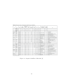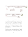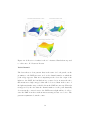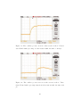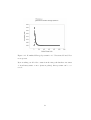
1
1
Abstract
The neutron is a subatomic Hadron of no net charge and a similar mass to
that of a proton. There is no direct way of measuring the presence or energy of a neutron, as when looking for a neutron, current radiation detection
equipment can only see charged particles created in a reaction, which has
had a neutron involved as a reactant. With the advancement of inorganic
and organic scintillating materials, specially designed to be used for radiation detection, it has become easier to detect these charged particles. With
this comes the need for more advanced pulse processing, in order to clearly
distinguish between electrical signals created in a detector, that have been
created by neutrons and those that have been created by other sources of radiation or electronic noise. This document focuses on the work done with a
set of specially designed scintillator panels, comprised of two types of scintillating material and the digital pulse processing preformed on them, in order
to distinguish between gamma and neutron pulses within a detector. One of
the materials is a plastic scintillator sensitive to gamma radiation whilst the
other is a Zn/S layer doped with 6 Li, which is sensitive to neutrons. Up until
now no one has successfully been able to separate pulses in one material relating to gammas and neutrons, this work should help towards changing this.
Contents
1 Introduction
4
2 Theory
2.1
2.2
2.3
2.4
2.5
11
Gamma and Neutron Raidation Deffinitions . . . . . . . . . .
11
2.1.1
Gamma Radiation . . . . . . . . . . . . . . . . . . . .
11
2.1.2
Neutrons . . . . . . . . . . . . . . . . . . . . . . . . .
12
2.1.3
Thermal Neutrons . . . . . . . . . . . . . . . . . . . .
13
2.1.4
Fast Neutrons . . . . . . . . . . . . . . . . . . . . . . .
13
Gamma Ray Interactions and Neutron Interactions . . . . . .
13
2.2.1
Gamma Ray Interactions . . . . . . . . . . . . . . . .
13
2.2.2
Compton Scattering . . . . . . . . . . . . . . . . . . .
14
2.2.3
Photoelectric absorption . . . . . . . . . . . . . . . . .
17
2.2.4
Pair Production . . . . . . . . . . . . . . . . . . . . .
17
2.2.5
Neutron Interactions . . . . . . . . . . . . . . . . . . .
18
Neutron
Li6
Interaction and Reaction Cross Section . . . . .
20
2.3.1
Reaction Cross Section . . . . . . . . . . . . . . . . . .
20
2.3.2
Neuton Li6 Interaction . . . . . . . . . . . . . . . . . .
21
Scintillation Detector Basics . . . . . . . . . . . . . . . . . . .
22
2.4.1
Luminescence . . . . . . . . . . . . . . . . . . . . . . .
22
2.4.2
Molecular Fluorescence Spectroscopy . . . . . . . . . .
23
2.4.3
Scintillator Materials . . . . . . . . . . . . . . . . . . .
23
Organic and Inorganic Scintillator Properties . . . . . . . . .
25
2.5.1
Organic Scintillators . . . . . . . . . . . . . . . . . . .
25
2.5.2
Organic Plastic Scintillators . . . . . . . . . . . . . . .
27
2.5.3
Light Output . . . . . . . . . . . . . . . . . . . . . . .
27
1
2.5.4
Time Response . . . . . . . . . . . . . . . . . . . . . .
28
2.5.5
Inorganic Scintillators . . . . . . . . . . . . . . . . . .
30
2.6
Spectroscopy . . . . . . . . . . . . . . . . . . . . . . . . . . .
32
2.7
Pulse Processing Techniques . . . . . . . . . . . . . . . . . . .
33
2.7.1
Pulses . . . . . . . . . . . . . . . . . . . . . . . . . . .
33
2.7.2
Analogue Pulse Processing . . . . . . . . . . . . . . .
34
2.7.3
Digital Pulse Processing . . . . . . . . . . . . . . . . .
35
2.7.4
Comparison of Analogue to Digital Pulse Processing .
35
3 Experimental Procedure and Detector Design
3.1
3.2
Detector Design and The Pixie4 System . . . . . . . . . . . .
38
3.1.1
Schematic . . . . . . . . . . . . . . . . . . . . . . . . .
38
3.1.2
Zinc Sulfide as an Inorganic Scintillator . . . . . . . .
39
3.1.3
AmBe Neutron Source . . . . . . . . . . . . . . . . . .
40
3.1.4
Pixie 4 System . . . . . . . . . . . . . . . . . . . . . .
42
Experimental Procedure . . . . . . . . . . . . . . . . . . . . .
44
4 Gamma Work
4.1
4.2
4.3
48
Detector Resolution Work . . . . . . . . . . . . . . . . . . . .
48
4.1.1
Detector Resolution . . . . . . . . . . . . . . . . . . .
48
4.1.2
Results . . . . . . . . . . . . . . . . . . . . . . . . . .
49
Collimated Cs Source Work . . . . . . . . . . . . . . . . . . .
51
4.2.1
Collimated Cs Source . . . . . . . . . . . . . . . . . .
51
4.2.2
Results . . . . . . . . . . . . . . . . . . . . . . . . . .
52
Gamma Work Discussion . . . . . . . . . . . . . . . . . . . .
55
5 Neutron Work
5.1
5.2
5.3
38
57
Oscilascope Trace Work . . . . . . . . . . . . . . . . . . . . .
57
5.1.1
Oscillascope Traces . . . . . . . . . . . . . . . . . . . .
57
5.1.2
Oscillascope Results . . . . . . . . . . . . . . . . . . .
58
Rise Time Measurment and Zn/s Gamma Sensitivity . . . . .
62
5.2.1
Rise Times . . . . . . . . . . . . . . . . . . . . . . . .
62
5.2.2
Ratio Results . . . . . . . . . . . . . . . . . . . . . . .
69
Pulse Shape Discrimination . . . . . . . . . . . . . . . . . . .
71
5.3.1
71
Conditions used for seperation . . . . . . . . . . . . .
2
6 Conclusions
75
7 Acknowledgments
77
3
Chapter 1
Introduction
The Discovery of Gamma and Neutron Radiation
The scientific community has been aware of radiation since the start of the
20th century, in 1900 French physicist Paul Villard, discovered gamma radiation whilst studying a piece of Radium but was not named so until 1903
by Ernest Rutherford. 17 years later in 1920, Rutherford, proposed the existence of an uncharged particle which would be found inside the nucleus of
an atom, to better explain the difference that was found between the atomic
number and atomic mass of elements. This theory was not popular as the
accepted opinion at the time was that a nucleus was only made up of protons and electrons. In 1930 Viktor Ambartsumian and Dmitri Ivanenko, two
Russian physicists proved that the nucleus could not be made up of protons
and electrons, but rather of protons and some other neutral particle.
During the year of 1931, an experiment was done by physicists Walther
Bothe and Herbert Becker which produced a highly penetrative type of radiation that was thought to be just another type of gamma ray radiation.
The results from this experiment were not clear or easy to interpret as such
there was no reason to believe this radiation was anything other then gamma.
However in 1932 Parisian scientists, Irene Joliot-Curie and Frederic JoliotCurie showed that if this radiation was incident on the substance paraffin,
the paraffin would eject protons of very high energy. Paraffin is a hydrogen
4
containing compound, if this new radiation was indeed gamma based, this
reaction should not occur thus suggesting that this highly penetrative radiation was not another form of gamma radiation, as previously thought.
It wasn’t until 1932 that Rutherford’s theory was finally proven by James
Chadwick. Whilst working at the University of Cambridge, Chadwick proved
that the gamma explanation for this radiation was not correct and instead
proved that the nucleus must be made up of a combination of protons and
another uncharged particle that had a similar but slightly different mass to
that of the proton. He called this new particle, the neutron. The neutron is
currently a hot topic for study in the field of radiation detection as it gives
further insights to the make up of atoms [1].
Scintillator Materials and Digital Pulse Processing
In recent years the quality of scintillator materials and the ability to process
the electrical pulses produced in them have increased and lead to better
quality of energy spectra. The combination of the two could lead to devices
that are better at detecting radiation which is good for a number of reasons,
one such reason in scanning vehicles at army checkpoints in order to locate
hazardous materials.
Security Applications
Rapiscan is primarily a radiation detection company who since 1993 have
installed over 70,000 products in over 100 countries. Their products range
from simple baggage and parcel inspection systems up to equipment specially
designed to detect explosive devices and nuclear material. Their systems are
in use in airports, government buildings, correctional facilities and even sea
ports. Rapiscan have developed a type of scintillation panel which consists
of one scintillation panel made of Zn/S doped with 6 Li, sandwiched between
two plastic scintillation detectors.
5
Figure 1.1: Simple RadNuke Schematic, the black section represents the
Zn/s layer
The overall design should allow for the detection of gamma rays and thermal neutrons. The plastic scintillators will pick up gamma rays whilst at the
same time moderating fast neutrons to slow neutrons so the 6 Li panel can
interact with them and detect the charged particles created. It is the goal
of Rapiscan to develop a detector system that uses digital pulse processing
to analyse an object that is placed in front of one of these panels. In the
end it should not only be able to tell if radiation is present or not, but from
the spectrum obtained it should also be able to identify the source. This
work documents the tests done on a set of similar panels using a Varity of
gamma sources and an Am Be neutron source. It all so details the digital
pulse processing techniques used in order to analyse the data acquired.
The main use for these types of panels is in security applications. Rapiscan
have several types of detector systems that are designed to scan vehicles at
army checkpoints and smaller ones that are designed to scan baggage. The
aim of these systems is to detect either harmful substances or items that
could be used as weapons. As this is such an important job these detector systems are all ways being worked on and improved. When no more
improvement can be done on the current existing panels, new ones are designed to compensate.
When detecting neutrons, it is the charged particles created in a reaction
that one looks for as opposed to the neutron itself as this is a lot easier to do.
In the 6 Li neutron interaction, two charged particles, an Alpha particle and
a Triton are produced with a respective Q value of 4.78 MeV. The reasons for
including the gamma detecting panels are two fold, the first is that gamma
6
ray spectroscopy is a handy tool when it comes to identifying radioactive
nuclei and the second is for a use of application reason. The probability that
an interaction occurs between two particles can be expressed in terms of a
reaction cross section, the higher the cross section of a material the more
likely an incoming particle is to hit a particle of that material and interact.
In the case were neutrons are the incoming particle, the cross section for 6 Li
(see figure 1.3) remains small until the energy of the neutrons decrease to
an energy of roughly 0.025 eV corresponding to slow neutrons [2]. Fast neutrons can still be detected and this is achieved through neutron moderation
which takes place inside the plastic scintillation panels through processes
such as scattering (see figure 1.4) to lower their energies.
Figure 1.2: Picture of the Rad-Nuke Vehicle scanning Detector System
The Rad-Nuke portal consists of a set of seven detectors as described before
all running in unison. As there is more then one detector, measures must
be taken so that the output viewed from one detector is the same as viewed
from all others, one thing to think about in this respect is the voltage supply
that is fed to each detector. It is this system that is looking to be improved,
7
the panels used for these experiments consist of just one gamma sensitive
panel and the Zn/S sheet however as the materials are the same anything
that is found using these panels, will be valid for the same detectors that
make up the Rapiscan Rad-Nuke portal. The panels are arranged in an arc
which the vehicle must drive through (see figure 1.2).
Figure 1.3: The reaction Cross Section for Li6 [16]
8
Figure 1.4: Scattering of Neutrons in a Moderator
The methods for detecting gamma radiation and slow neutron radiation differ when using scintillation detectors, as the mechanism required for gamma
detection, requires the incident gamma rays to have energies of at least a
few eV to work. Slow neutrons are defined as having energies of anything
below and up to 0.5 eV which is known as the Cadmium cut off point, this
therefore means that slow neutrons have too small of an energy to use the
same detection methods as what is used when looking at gamma radiation.
A detector design used to successfully measure both types of radiation is
to join together two different scintillating materials, one of which is gamma
sensitive, (In this case the plastic scintillator) and the other which is sensitive to slow neutrons (the Zn/S sheet). Both materials are then joined to
the same photomultiplier tube which takes the light pulses being created
from both scintillators and converts them into electrical signals.
9
The one problem that arises from this method is that the form that these
electrical pulses due to gamma and neutron radiation take, do not relate to
each other in anyway apart from the fact that they are both representative
of the initial incident radiation that created them. This means that any
spectrum produced by simply measuring the amplitude of these pulses and
placing then on a typical counts Vs energy graph, will produce a spectrum
that has both gamma and slow neutron events but appearing in wrong channels. A Pulse of height x produced in the Zn/s layer will not have the same
energy as a Pulse of the same height produce in the Plastic layer, due to
reasons such as not being created by the same mechanism and being created
in different materials. A simple computer program will not know this so it
will place both events in the same channel. The main goal of this project is
therefore to design a way to distinguish between gamma and neutron pulses.
Using analogue methods to form the pulses this distinguishing can not be
done, however by using more advanced digital pulse processing techniques,
this can be done. By looking at the different forms the pulses take in the
system, such as different widths and amplitudes, one can tell pulses apart,
this is known as pulse shape discrimination. It is the aim of this experiment
to see if it is possible to tell the difference between the two types of pulse and
apply different energy calibrations to them resulting in a complete spectrum
that can be obtained with only one set of detector readings. The main difference that this method will be concerned with, is measuring the different
rise times of the two pulses as theory would suggest the pulses created by
the thermal neutrons, should have a noticeably longer rise time. The digital
system will allow this difference to be detected.
10
Chapter 2
Theory
2.1
2.1.1
Gamma and Neutron Raidation Deffinitions
Gamma Radiation
When a heavy nucleus undergoes either alpha or beta decay, the daughter
nucleus is often left in a higher, exited energy state. If this state is such
that the difference between the current energy level and the ground state is
less then the energy needed for fission, the daughter nucleus will de-excite
by emitting a high energy photon [1]. Gamma rays form when a nucleus
drops from an excited state back into a lower state creating light (Gamma
Ray Photon), this light can be absorbed by certain types of radiation detection equipment to measure and record the radioactive events. X-rays have
similar wavelengths and energies to gamma rays however they are emitted
by electrons outside of the nucleus.
11
Figure 2.1: A nucleus decaying by emission of a gamma ray, Protons are red
and neutrons are blue [3]
2.1.2
Neutrons
The neutron is a subatomic Hadron of no net charge and a similar mass to
that of a proton, in general all nuclei of atoms apart from hydrogen consist
of a combination of neutrons and protons. Neutrons are generally detected
by looking for the energetic particles such as alpha particles and protons
that are created in nuclear reactions were a neutron has been the catalyst.
The majority of neutron detectors are comprised of a target material that is
sensitive to neutrons (such as Li), coupled to a standard radiation detector
such as a scintillation detector. Neutrons that are not bound in an atom
are unstable and can undergo beta decay, usually in experiments it is these
free neutrons that are used. The cross section for neutron interactions in
most materials is dependant on the energy of the neutron with lower energies having a better chance to interact. Because of this different methods
are used to detect different types of Neutrons which fall into two categories
know as thermal and fast neutrons. [4]
12
2.1.3
Thermal Neutrons
Neutrons that have energy less than 0.5 eV are classed as slow neutrons, it
is these neutrons that are found in modern day nuclear reactors and it is
the purpose of most detectors in this field to measure the neutron flux. The
neutrons having such a low energy cannot be detected by methods such as
proton recoil however because their energies are so low, the reaction cross
section for certain materials becomes large enough for a reaction to occur
more frequently. This leads to the admittance of charged particles that can
be measured with the use of standard radiation detectors.
2.1.4
Fast Neutrons
Fast neutrons are classed as high energy neutrons and as such the methods
used for detecting them are not the same as for slow neutrons, as the reaction cross section is now too small to acquire any good data. Instead a
method known as fast neutron scattering is used, this is where the fast neutron scatters lighter nuclei that can be detected. The neutron imparts most
(if not all) of its energy on the lighter nuclei, the recoil nuclei that result
from elastic scattering from ordinary hydrogen are called recoil protons and
it is these that a lot of detectors are based on.
2.2
Gamma Ray Interactions and Neutron Interactions
2.2.1
Gamma Ray Interactions
Although there are many known ways that gamma rays can interact with
matter, there are only three main ways that they do:
• Compton Scattering
• Pair Production
• Photoelectric Absorption
13
All these processes work in similar ways in that the complete or partial
transfer of the energy associated with the gamma ray photon is transferred
to an electron within the target material. This sudden transfer of energy is
in direct contrast to charged particles that transfer their energy over a series
of collisions with a multitude of atoms within a material. [5]
2.2.2
Compton Scattering
In low Z materials such as liquid scintillators or certain types of plastic scintillators, gamma rays interact by Compton scattering [6], and so the general
energy spectrum consists of a Compton continuum and edge, but no photo
peak. In a scattering event, a photon collides with an electron within the
target material depositing part or all of its energy to the electron before
moving off at a new angle. The electron absorbs the energy lost by the
photon and recoils with a kinetic energy Ee :
Figure 2.2: A photon of wavelength λi comes in from the left, collides with
an electron at rest, and a new photon of wavelength λf emerges at an angle
θ [7]
The conservation of energy means that the energy of the incoming photon
14
Ep added to the energy of the electron Ee summed is equal to that of the
two after collision such that:
Ee + Ep = Ee′ + Ep′
(2.1)
By taking into account that photons have momentum and that the energy
of a photon is given by
E = hν
(2.2)
were h is Planck’s constant and ν is the frequency of the wave, one can
derive an equation for the change in energy or wavelength that the incident
photon has after the collision with the electron. If done correctly the following formula is found.
λf − λi =
h
(1 − Cos(θ))
Me c
(2.3)
where
λf is the wavelength of the scattered photon,
λi is the initial wavelength,
h is Planck’s constant,
Me is the rest mass of the electron,
c is the speed of light
θ is the scattering angle.
There are two extreme cases of scattering which make up the lower and
higher ends of the Compton continuum.
1. Small angle scattering or grazing angle when θ = 0, cos(θ) = 1. In
this circumstance Ep′ is almost the same as Ep and so Ee′ = 0. The
recoiling electron has basically no energy and the recoiling photon is
scattered at a minimal angle resulting in very little energy loss.
15
2. A head on collision where θ = π. In this circumstance the photon
is backscattered along the same direction that it was incident on the
electron on. The electron itself recoils along the direction of incidence.
In this case the recoil electron energy is given by.
EMAX = Ep
1
2Ep
Me c2
2E
+ Me cp2
(2.4)
This represents the maximum detectable energy for this mechanism of detection and corresponds to the Compton edge part of the spectrum. As
the energy the detector can detect is then within a range of many possible
energies, a spectrum forms with a characteristic known as a Compton continuum, the following is an example of this (with a photo peak). The photo
peak is not always present but if the process that has occurred is Compton
Scattering, the continuum will be.
Figure 2.3: Example of Am-Be gamma spectrum with Ideal Compton Continuum [8]
16
2.2.3
Photoelectric absorption
In the photo electric effect, an incident photon undergoes a reaction with a
target atom in such a way that the incident photon disappears completely.
An atom will absorb the incident photon and eject a new photo electron
from an electron shell, in the case were the incident photon is a gamma ray
photon, this will most likely be from the most tightly bound K shell. As the
mechanism for this reaction requires the whole atom, it can not take place
with a free electron. The photo electron that is created has an energy given
by
Ee = hν − Eb
(2.5)
Where Eb represents the binding energy of the photo electron from it’s original shell. This ejection of a photo electron creates a vacancy in the shell it
came from which can be filled by a free electron. This can come from either
outside or inside the atom creating a characteristic X-ray, as such the above
process can be repeated if the atom then absorbs this X-Ray.
This mode of interaction is the most common for gamma rays of low energy,
especially if the target material is a high Z material, as such detectors designed to measure only gamma events, are often made of high Z materials
such as Germanium.
2.2.4
Pair Production
If a gamma ray has more than twice the energy of the rest mass energy
of an electron, the process of pair production is energetically possible but
not nessercellary dominant, it does not become so until the gamma rays
reach MeV of energy. This reaction takes place within the Coulomb field
of a nucleus, as such it can not happen without the presence of an atom.
In this reaction the gamma ray photon disappears completely, like in the
photoelectric absorption mechanism however this time an electron-positron
pair are made. Any energy above 1.02 MeV that the incident photon had is
17
transferred to kinetic energy between the electron and positron.
Once the positron slows down enough within the material it will annihilate
creating two annihilation photons which are both measured in detectors. In
a low Z material, the photoelectric cross section is too low for a photo peak
to emerge, therefore the only information you can get from a gamma ray
interaction is the spread of energy that the gamma ray electrons can take
via the most dominant gamma ray interaction, in this case the Compton
scattering events.
2.2.5
Neutron Interactions
As with gamma rays, neutrons carry no net charge so they do not interact
with matter via the coulomb force which is the dominant means of interaction for charged particles and electrons. However neutrons are also more
penetrative then gamma rays and can pass through many cm of materials
without undergoing any sort of interaction, this means that they are not
seen by common sized gamma detectors [4].
For this reason when trying to detect neutrons it is the charged particles
created in a reaction were a neutron has been one of the reactants that a
detector looks for. When a neutron does interact, it is with the nucleus of
an atom and itself will either disappear completely or have its energy and
direction of travel changed severely. Often the created radiation takes the
form of heavy charged particles emanating either from the nucleus of the
target material itself or a neutron induced nuclear reaction.
Slow neutrons tend to interact with a target in one of two ways, the first
is through elastic scattering whilst the second is by neutron-induced events
within the target material. Because of the relatively small amount of kinetic energy a thermal neutron has, hardly any energy can be transferred
to the nucleus of an atom in elastic scattering, this fact means slow neutron detectors are not designed to detect neutrons this way but rather in
18
the more probable case of interaction, were a neutron reacts with a target
nucleus and creates a set of heavy charged particles that can themselves be
seen. The types of favoured reactions that can occur are (n,a), (n,p) and
(n,fission) as charged particles are created however another type of reaction
can occur using foil targets however the reaction creates a second type of
radiation often gamma, making this reaction great for neutron shielding but
not nessercellary for neutron detection.
A neutron
collides with a
target atom
The neutron is absorbed
into the atom
The unstable
atom then splits
releasing two
heavy charged
particles
Figure 2.4: Diagram of Neutron-Induced Events
Fast neutrons with higher energies, must be detected in different ways as the
probability for neutron-induced events drops drastically with the increase of
energy. The main reaction now becomes inelastic scattering, where the created product is a recoil nucleus that if given enough energy will de-excite
via the emission of a gamma ray. A neutron will transfer most of it’s energy
to a target of similar mass making materials made of hydrogen the best type
for detectors based on this reaction, subsequently, heavier nuclei do not perform as well. In this sense the material is acting as a moderator and as each
collision takes a portion of the neutrons energy, hydrogen is considered the
best as it can take all of the energy in one collision.
19
2.3
Neutron Li6 Interaction and Reaction Cross
Section
2.3.1
Reaction Cross Section
The probability of an interaction occurring between some sort of incident
radiation and a target atom, electron or nucleus can be expressed in terms of
a reaction cross section. An incident radiation will have a flux of Io , consider
this beam arriving at an absorber at right angles to it. The absorber itself
has element thickness dx and surface area Q. The transmitted flux, (or the
amount of radiation per unit area per unit time) that was not absorbed, can
then be expressed as Ix = Io + dI , where dI is the change in Flux. The Volume of the element can be expressed as Q.dx, if the materials atomic density
is N atoms per unit volume, the element then contains N Q.dx atoms. Each
atom has a removal cross-section J, nuclear overlap is negligible, we have a
total target area of removable as N QJ.dx. [10]
dx
Io
Area
Incident Flux
Ix = Io + dI
Transmitted Flux
Q
Figure 2.5: Reaction Cross Section Diagram
Working this through to its conclusion results in.
20
Ix = Io exp(−µx)
(2.6)
Where µ is the linear attenuation coefficant and is simply given by
µ = NJ
(2.7)
This coefficient can be used to work out the mean free path, λ, of the material
and is given by λ =
X
λ
1
µ
equation 2.6 can then also be written as Ix = Io exp −x
λ .
is therefore the absorber thickness expressed in an amount of mean free
paths. Ix /Io gives the fractional amount of radiation passing through a material, the fraction absorbed is then simply 1 − Ix /Io which is the intrinsic
detection efficiency, for ideal detection, you want this value as close to one
as possible. Nuclear cross sections are expressed in Barns where 1 Barn
= 10-28 m2 , corresponding to the circular cross sectional area of what ever
atom the material is made of.
Particles have a de Broglie Wavelength given as λ =
h
mv
were mv is the linear
momentum of the particle. The lower the energy therefore the bigger the
wavelength, when this wavelength becomes bigger it has more of a chance
of interacting as it becomes larger than the nuclear radius of the atom, for
neutrons to be detected in this method they need to have low energies, the
best results for this are achieved with thermal neutrons.
2.3.2
Neuton Li6 Interaction
There are few atoms that make for good neutron detectors where the desired
reaction results in the creation of two charged particles, the best atom to
use is that of He. The reaction for He is the following [4].
3
He(n, p)[3 He2 +1 n0 =3 H1 +1 H1 + 0.764M eV ]
(2.8)
However due to He benefits it has become highly popular and as it is used
in many other areas, not just in radiation detection, it is vary costly to
21
create large detectors from it. An alternate atom to use ( and the one this
paper focuses on ) is Li6. The reaction for a neutron with Li6 is the following.
6
Li9 (n, a)[6 LI3 +1 n0 =3 H1 +4 He2 + 4.78M eV ]
(2.9)
In this reaction, the neutron is absorbed and creates two charged particles
that have similar energies, one is an alpha particle, whilst the other is a
Triton. Li is much cheaper than He so could be a viable alternative for
large scale neutron detectors if it is proven to be good enough. The reaction
cross-section for thermal neutrons, all though not as good for He, is still
good as at low energies the cross section increases, a graph of this can be
seen in the introduction. This sort of reaction all though possible is highly
unlikely to work for fast neutrons, however as neutron energy increases the
elastic-cross section for neutrons increases, making detectors that work on
the principles of proton recoil are used.
2.4
2.4.1
Scintillation Detector Basics
Luminescence
Luminescence is the term given to the emission of light from a substance.
This process occurs when an electron in an excited state, loses energy by
emitting a photon and drops back down to the electron ground state. Luminescence can only be described using quantum physics and not in classical
terms, as quantum physics states that the possible energy values a system
can take, are determined by its internal properties, i.e. it’s structure. Often
the emitted light will have slightly less energy than that of the difference
between the two energy states, this energy however is still characteristic of
the material, so a form of luminescent spectroscopy can be done from looking at the emitted light. This is known as the first law of luminescence and
was formulated by Stokes in 1852. The law states “The wavelength of luminescence excited by radiation is greater then the wavelength of the exciting
radiation.” [11]
22
Luminescence Spectroscopy is the name given to three related spectroscopic
techniques.
• Molecular fluorescence spectroscopy
• Molecular phosphorescence spectroscopy
• Chemical luminescence spectroscopy
2.4.2
Molecular Fluorescence Spectroscopy
Particles have a set of different states known as energy levels. In the case of
an electron in an atom, the higher energy states relate to the electron itself
having a higher energy. Fluorescence Spectroscopy relates mainly to the
vibrational states and the electronic states. Normally a particle will consist
of a ground state (minimum energy) and a set of excited electronic states
which have vibrational states between them. In practice a particle will be
excited from the ground state to an excited state through the absorption
of a photon, it will then begin to loose energy through collisions with other
particles until it reaches the lowest vibrational level within the current electronic level. At this time to drop back down to a lower excited state, a
photon must be emitted. As the particle can drop back down to any of the
vibrational states in the lower level a set of different photons with different
wavelengths can be emitted. It is these differences that are measured in
order to determine the structure of the different vibrational states. In an
experiment a single wavelength beam can be used to excite a sample and
the fluorescence measured to produce emission spectrum. This spectrum
can tell you what material the sample is if you do not know.
2.4.3
Scintillator Materials
Scintillation is the term used when specifically talking about the luminescence that is produced when ionising radiation is incident on a scintillation
material.
23
Figure 2.6: A basic Scintillator Detector Design [12]
A scintillator is a material that when struck by a form of ionising radiation, absorbs the energy from the particle and then readmits it as light, this
process is know as luminescence. This property can be used in radiation detection, when a scintillator is coupled to a photomultiplier tube a scintillator
detector is made. The light emitted from the material is again absorbed by
the PMT and emitted as electrons via the photoelectric effect. The multiplication of these photoelectrons can then be turned into an electrical signal
that can be analysed resulting in the formation of data corresponding to the
initial energy of the photon that is emitted from the material.
Figure 2.6 shows a schematic of a scintillator detector, incident photons
strike the photo cathode material and create electrons via the photoelectric
effect, these electrons are then accelerated towards the first dynode which
is held at some positive voltage, increasing in energy as they travel. Once
they strike the dynode itself, more low energy electrons are created which
are once again accelerated towards the second dynode which is held at a
higher voltage then the first. This process is repeated until the electrons
reach the anode were the accumulation of charge is converted into a measurable electrical signal.
This Signal can be amplified by changing the voltage that is supplied to the
PMT by increasing the voltage you increase the signal but at the cost of a
lower signal to noise ratio.
24
The main properties an ideal scintillation material should have are the following.
1. It should convert the energy of the incident charged particles into
detectable light with a high efficiency.
2. This conversion needs to be linear, the light intensity created should
be proportional to the initial energy over a wide range.
3. The material should be transparent to wavelengths of its own emission
as to avoid re absorbing.
4. The decay time of the created light should be short so fast pulses can
be created.
5. The material itself should be good quality and easily manufacturable.
6. The index of refraction of the material should be close as possible to
that of glass to allow the best coupling to a PMT.
No one material can fit all 6 of these points, so often a compromise must be
made between them.
2.5
2.5.1
Organic and Inorganic Scintillator Properties
Organic Scintillators
The process of fluorescence in organics comes from the transition in energy
levels of a single molecule as such the physical state of the system plays no
part in the process [4]. This is in direct contrast with inorganic scintillators
that require a regular crystalline lattice as a base to achieve the scintillation
process. The energy levels of an organic molecule are represented by a system known as the pi-electron structure. The most stable state of a molecule
is known as the ground state and is the lowest energy a molecule can have.
It is represented by the notation S00 . The first 0 in this notation relates to
25
the singlet state which the molecule is in (Spin 0 for this case). Each singlet
state can be divided into a set of vibrational states that have a separation
of roughly 0.15 eV. S00 therefore relates to a spin of 0 with the lowest vibrational state, S01 relates to the next highest energetic state which is one
vibrational state higher then the ground state. S02 is one more vibrational
state then S01 and so on. A molecule can be excited into a higher state
by the absorption of kinetic energy from a charged particle, however if it is
excited into one of the vibrational states within S0 it will de-excite through
internal mechanisms that release no radiation. This structure can be seen
in figure 2.7 [4].
For light to be emitted, the transition must be between singlet states e.g.
S1 to S0 , typical energy gaps between adjacent singlet states are 3 to 4 eV.
Due to the fact that the energy spacing between vibrational states is large
when compared to the average thermal energies a molecule is in (0.025 eV)
a molecule in a standard situation will be found in the ground state and
needs something external to excite it into a higher one. The main source
of light (fluorescence) that detectors measure, comes from the transition in
energy from S10 to one of the Vibrational states of S0 . The time in which
it takes a newly excited state to decay back down, in an organic material
is short, usually a few nanoseconds making the prompt scintillation component relatively fast.
Figure 2.7 helps to explain why organic materials are useful as the energy
of the emitted light, tends to be less then what it takes to excite S0 to S1
meaning it full fills rule 3 of what makes a good scintillator. Some radiationless de-excitations can still occur from the S1 to S0 state and these all
fall under the term quenching but this is not normally an issue.
26
Figure 2.7: Energy States within a Molecule [13]
2.5.2
Organic Plastic Scintillators
A solid plastic scintillator can be created by dissolving an organic scintillator
in a solvent and then polymerized. Plastic scintillators are often the cheapest solution to simple gamma ray detection. This is because they are cheap
and often the only solution when it comes to making large scale detectors
designed to scan large areas as costs would rise significantly if the detector
was made from anything else. There are a few drawbacks however when
creating such large plastic scintillators, one is that the case of self absorbing
its own light may no longer be negligible and the second is the light intensity
may change significantly as it moves through the plastic due to attenuation.
2.5.3
Light Output
Only a portion of the kinetic energy lost by a charged particle in a scintillator is converted into light energy. The amount of energy transferred relates
to both the type of incident particle and its energy. For the case of electrons,
the response to energies above 125 KeV is linear, the response for charged
particles such as alpha particles, is always less for equivalent energies, see
figure 2.8. As initial energies increase, the response of the two begin to come
together however there is still a difference, at low energies this difference is
27
as much as 10 times bigger. It is important to remember this fact when using an organic material to detect both types of radiation as the light pulses
produced in the material will be different although they could be representative of the same energies. It is for this reason that more complicated pulse
processing is needed to properly distinguish between them.
Figure 2.8: Light Yield Comparisons, alpha particles fall roughly on the
same line as the protons do [14]
2.5.4
Time Response
In organics luminescent states are formed instantly and only prompt florescence is present, therefore the form that a typical light pulse takes in an
organic material can be thought of as having a sharp rise time, followed by
a exponential decay. The following is a table of common organic scintillator
materials and their associated properties.
28
Figure 2.9: Organic Scintillator Materials [4]
29
2.5.5
Inorganic Scintillators
The structure of the crystalline lattice in inorganic scintillators, is what determines the scintillation mechanism. In a crystal, electrons can only occupy
discrete energy levels in the lower energy band (Valance Band) or the upper
energy band (Conduction Band). Electrons in the valance band are bound
at lattice sites and can not move throughout the crystal, however if the
electrons have sufficient energy they can leave the valance band and enter
the conduction band leaving a hole behind in the valance band. Whilst in
the conduction band the electron is free to move around, any free electron
that then comes close to the produced hole can de-excite by emitting a light
pulse and be re absorbed into the valance band. There is an energy area
between the two bands known as the forbidden band gap were no electrons
can ever be found meaning that the light produced can only take discrete
energy levels representative of the band gap [4].
To maximise the chance of this process occurring, impurities are often added
to the inorganic crystal, these activators create sites within the lattice were
the traditional band gap is modified creating sites within the forbidden band
gap that electrons can occupy. It is these impurities which determine the
structure of any measured energy spectra. Figure 2.10 is a table of some of
the more common inorganic scintillator materials along with their properties.
30
Figure 2.10: Inorganic Scintillator Properties [4]
Included in the table is the properties of Zn/S which is the material the
second scintillator is made of, the pulses that come from this material have
the best pulse amplitude of all of the ones listed and all though blank in
this table, it has one of the highest light yields. By just looking at the two
tables for organic and inorganic properties, it can be seen that their properties vary by a great amount, for example the decay times in the inorganic
materials are a lot smaller then those of the organic ones, coupled in with
the light attenuation in the organic material it can be seen that the pulses
created will not be the same.
31
2.6
Spectroscopy
A gamma ray photon carries no net charge and as such does not cause any
ionization or excitation within materials that it passes through. This means
that for a gamma ray to be detected in something such as a scintillation
detector, it must first undergo an interaction that transfers all or part of
the photon energy, to an electron within the detection material. The type
of reaction involved is a sudden change/transfer in energy as opposed to the
slower method of slowing down heavy charged particles through multiple
collisions within the target material. Due to the mechanics of these interactions, it is only the newly formed gamma ray electrons that allow one to
determine the nature of the incident gamma ray photons as they themselves
are not seen by the detector.
The maximum energy one of these electrons can take is equal to the energy
that the incident photon had, this does not mean however that the detector
will always register this or at all, it all depends on how the detector is made.
A good scintillation detector must first do two things, it must be able to
react with the incident gamma ray photons, with a high enough probability
to create the new gamma ray electrons, a material that is good at this is
known as a conversion material. The second function then must be for it
to act as a detector for these newly created electrons. This can be done by
either having one material to do all of the work, or two joined together that
each do one of the two tasks.
FWHM is a number used to express detector resolution. This value is simply
the width of a photo peak (given in eV) at half of its amplitude. Detector
Resolutions are usually given in terms of gamma ray energies, for example
a Sodium Iodide detector could be said to have a resolution of 9 KeV at
611Kev corresponding to a Cs137 gamma ray. This means that if two energies are more than 9 KeV apart around 611 KeV, the detector should be
able to tell the two apart and show two separate peaks. Detector resolution
can also be expressed as a percentage by taking the FWHM and dividing
by the gamma ray energy.
32
Figure 2.11: Full Width Halh Maxima Example
2.7
2.7.1
Pulse Processing Techniques
Pulses
A pulse is the electrical representation of a charge created in a detector when
a photon or a particle interacts with the material of a detector. This charge
is usually proportional to the initial energy of the photon/particle that was
used to create it. Each event counts as one pulse so a series of pulses can be
used to measure the count rate of a source, or by measuring the amplitude
of the individual pulses, produce an energy spectrum that is representative
of the radioactive source. A pulse can be broken down into segments that
describe what it looks like.
33
Figure 2.12: Example of a Signal Pulse from a PMT
Above is an example of an electrical pulse that has been recorded using digital pulse processing methods. The amplitude of this pulse (21800 arbitary
units) is what is used to determine the energy of the incident particle that
was used to create it. A program will measure the amplitudes of several
pulses and place those with higher amplitudes in higher numbered channels
than those with lower amplitudes. Users can then set an energy calibration
to these channels if required. The section marked in yellow is known as
the rise time, this is the time it takes for the electrical signal to reach its
maximum amplitude, the red section is known as the decay time.
2.7.2
Analogue Pulse Processing
Analogue pulse processing uses electronic equipment to process electronic
signal pulses that arise when a radiation detector is in the presence of a
radioactive source. The signal from a pre-amplifier output goes to a shaping
amplifier and then on to a multi channel analyser. The shaping amplifier
works to shape the input pulse so that an accurate measurement of the pulse
height can be measured. Pulse shaping reduces the overall noise of a signal, it works towards reducing pulse pile up and removes the direct current
baseline [15].
34
2.7.3
Digital Pulse Processing
A DPP digitises the signal from a pre-amplifier output, applies digital pulse
processing techniques onto the signal which then allows it to accurately measure the amplitude of the signal pulse digitally, this value can then be binned
into its histograming memory so that an energy spectrum can be built. More
advanced DPPs can also record the form that each incident pulse takes [15].
Traditional analogue circuitry will not allow you to do any sort of pulse
analysis as the pulse shape is not recorded at any point, only the amplitude
of the pulse is needed. With the improvement of fast analogue to digital
converters however it is now possible to record each individual pulse that is
created, this allows you to play back data acquisitions at a later time with
certain restrictions added to how the program treats them. These restrictions can be found by first manually analysing the pulses that have been
created.
2.7.4
Comparison of Analogue to Digital Pulse Processing
DPPs can be used to replace many of the standard components in an analogue processing system such as the multi channel analyser, any pulse shaping logic devices and many more auxiliary circuitries. They do this by
making use of software which in commercial DPPs can be found written
into the hardware or by running the digitized signals through software that
the user has created in another program.
Figure 2.13 shows a comparison of the components used between a digital
and an analogue processing system.
35
Figure 2.13: Schematic of analogue/digital processing systems
The block diagram for the analogue process shows the basic set-up of any
normal processing system. It shows the detector, pre-amplifier, shaping
amp, MCA and computer. With this many extra components can be added
to further increase the ability to shape the pulses and acquire data. In comparison the block diagram for the digital process shows a lot less components
as the analogue to digital conversion takes place sooner than it does in the
analogue instrument setup. The conversion occurs straight after the preamplifier as opposed to after the shaping amp, this allows all of the pulse
shaping and analysis to be done within the DPP itself saving on space and
more importantly time.
With traditional circuitry only a finite number of shaping variables can be
achieved and this is usually done by turning a dial on the front of the shaping amp to the desired amount. More advanced users can manually replace
resistors and capacitors within the circuitry of the amplifier to obtain other
36
values but this can be delicate and time consuming work. In a DPP all
this shaping is done in real time by software so any number of values can
be chosen as long as the software permits it, this also allows other shaping
techniques that are not possible or easily done using analogue equipment
such as trapezoidal shaping.
37
Chapter 3
Experimental Procedure and
Detector Design
3.1
3.1.1
Detector Design and The Pixie4 System
Schematic
The experiments carried out within this paper, have all been conducted using at least one of a set of specially designed scintillation panels which have
been built in order to detect and distinguish between incident gamma rays
and incident neutron radiation.
The setup consists of a total of 4 panels, the first of these panels is comprised of two separate scintillation materials. One of these materials is a
solid plastic scintillator that can detect gamma radiation, whilst the other
(which is placed on top of the plastic) is a Zn/S layer doped with Li that can
be removed for testing purposes and is designed to detect neutrons. A photo
multiplier tube is attached to the plastic scintillator and is the device used
to convert any light pulses from the plastic or Zn/S into electrical pulses for
measurement.
The surface area for each material measures 50cm by 30cm with the plastic
layer having a depth of 1” and the Zn layer a depth of 1mm. The second
detector is identical to the first, however the depth of this panel is now 1.5”
38
REV#
A
DATE
03-19-10
ALTERATIONS
INITIAL RELEASE
BY
CRH
SILICONE GREASE
VISILOX, P/N 03-5432
BLACK RTV
P/N 03-6003
VITON O-RING SIZE 214,
McM# 9464K35
SCREW ¼-20 X ¾“
F/H M/S SS, 4 EA
SHV,-HV
12“
BNC
SCREW, 4-40 X 3/8“
BT/H M/S SS, 4 EA
TUBE BASE
P/N 5435-290-1
BLACK RTV
FILLET
R6094 PMT
NEG-HV PREPPED
PER 4467-1014
FOIL & VINYL
WRAPPING ON ALL
BUT ONE LARGE FACE
BACK CAP
P/N 7467-304
HOUSING
ASSEMBLY
P/N 2467-301
EJ-200 PLATE
1½“ X 7.9” X 19.7
(38mm x 299mm x 500mm)
ELJEN TECHNOLOGY
TOLERANCES
.XX
± .010
.XXX ± .005
ANGLES ± 0.5
DATE
INIT
03-19-10
REV
DETECTOR ASSEMBLY
M550-15x79x197-2
o
P/N:
4467-BEND
19-MAR-10
SERIES
467
SHEET
A
BEND
M550-15x79x197-2 ASSY.CDR
Figure 3.1: Schematic of the Type of Panels used in all experiments written
about in this paper.
but apart from this the two are identical. The third and fourth detectors
are again identically to the first two having the same depths of 1” and 1.5”.
However this time the plastic scintillator has been replaced with an unactivated plastic that can not detect any form of radiation, in theory this then
acts purely as a light guide for any light pulses being created in the Zn/S
layer due to neutrons.
3.1.2
Zinc Sulfide as an Inorganic Scintillator
Zinc sulfide was one of the earlier materials used as a basis for inorganic
scintillators as its high light yield was vary desirable. However as it is only
available as a polycrystalline powder, it is limited in that it can only be
made into thin screens as too thick and the material would once again break
rule 3 of what makes a good scintillator.
The pulses created in these panels come from both the two types of scintillator under different mechanisms (see theory). Theory would suggest that the
rise times of the pulses will be different. For gamma rays this time should be
39
roughly 1 µs where as for the slow neutrons it should roughly be 10 µs.The
reason the rise times of the two pulses differ is because the charge recorded
by the gamma rays is created when a gamma ray excites an electron to a
higher state within the plastic and decays back down to emit light where
as the light in the Zn/S layer is created when a slow neutron is absorbed
by a Li atom and a alpha and triton particle are created and then again
reabsorbed into the Zn/S. Further more this light has to then pass through
the plastic Scintillator layer to reach the PMT resulting in a pulse with a
longer rise time (see theory for more details).
Without digital pulse processing, pulses with the same amplitude will be
binned into the same energy channel in a spectrum, however if they come
from different sources they will not be representative of the same energies.
By measuring the rise times of the pulses and applying different energy calibrations to the longer rise times than the shorter, this problem could be
solved.
3.1.3
AmBe Neutron Source
A standard laboratory source (and the one used for these experiments) of
neutrons is the AmBe generator. This comprises a high activity (GBq)
241 Am
source (a long lived alpha-emitter with T1/2 = 433 years) that is
mixed with beryllium (Be) powder and placed in a sealed can. Neutrons
are generated through the 9 Be (alpha) reaction with energies in the range
0-11 MeV. For reference, an 18.5 GBq AmBe source has an output of 106
neutrons per second. AmBe sources are typically placed in a water tank
such that the fast neutrons are slowed down to thermal energies through
multiple scattering with hydrogen in the water molecules. This occurs over
a distance of a few cm and generally results in neutron capture through the
reaction 1H(n,alpha)2H in which deuterium is formed[6].
40
Figure 3.2: Calculated neutron energy spectrum from various actinide-based
sources. The red section is the energy spectrum of the neutron source used
in these experiments
41
Figure 3.3: [Schematic diagram of the Am-Be (source B) neutron source
mounted in the water tank, and the adjustable air pipe.
3.1.4
Pixie 4 System
Because of the complexity of the signal pulses being produced within the
PMT from the different light sources, digital pulse processing is needed in
order to separate out the pulses relating to gammas and neutrons. To do
this the Pixie4 system, a pulse data acquisition system created by the company XIA has been used to record the raw pulse data from the experiments
where both gamma and neutrons are present.
“The DGF Pixie4 is a 4-channel all-digital waveform acquisition and spectrometer card based on the Compact PCI/PXI standard for fast data readout to the host. It combines spectroscopy with waveform capture and on-line
pulse shape analysis. The Pixie4 accepts signals from virtually any radiation
detector. Incoming signals are digitised by 14-bit 75 MSPS ADCs. Waveforms of up to 13.6 µs in length for each event can be stored in a FIFO.
The waveforms are available for on-board pulse shape analysis, which can be
customized by adding user functions to the core processing software. Wave42
forms, timestamps, and the results of the pulse shape analysis can be read
out by the host system for further off-line processing. Pulse heights are calculated to 16-bit precision and can be binned into spectra with up to 32K
channels. The Pixie4 supports coincidence spectroscopy and can recognize
complex hit patterns.
Data readout rates through the Compact PCI/PXI backplane to the host
computer can be over 100Mbytes/s. The PXI backplane is also used to distribute clocks and trigger signals between several Pixie4 modules for group
operation. With a large variety of Compact PCI/PXI processor, controller
or I/O modules being commercially available, complete data acquisition and
processing systems can be built in a small form factor (more details on the
Pixie system can be seen in the Appendix).” [9]
To process the data obtained by the Pixie system, the data that contains
the raw pulse files can be replayed back through an open MCA program.
This program allows you to measure certain aspects of a pulse. The pulse
shape discrimination that was used in these experiments was to measure the
rise times of the pulses between 10% and 90% of the pulse amplitude. The
measured values are then stored along with the pulse amplitude at this measured rise time, figure 3.4 shows a picture of this idea, what these rise times
are used for is father described in the up coming experimental procedure
section. By manually setting what range of rise times the pulses are likely
to take along with the amount of data channels the program should assign
to these values, the program can bin this data in accordance.
43
Figure 3.4: Rise Time Measurment for Pulse Shape Discrimination
3.2
Experimental Procedure
Gamma Source Experiments
For the initial run of gamma experiments where neutrons were not present,
no digital pulse processing was needed, instead, traditional analogue pulse
shaping methods were used. The gamma experiments were designed primarily to characterise the detectors as this had not been done before. A set of
gamma sources, Cs, Co and a Na source were used. In each experiment one
of the sources would be placed over the centre of the panel being tested, data
acquisition would then commence for the same amount of time per source.
For the detector resolution the two Activated Perspex panels, which only
differed by thickness were used. One of the Panels was 1” thick whilst the
other was 1.5”. Each panel was individually connected to a preamp then to
a timing filter amp which had a constant integration time of 200ns and a
constant differentiate time of 100ns set. The aim was to see how detector
resolution varied around a Cs photo peak when the voltage to the photomultiplier tube was itself varied. A range of 600 V to 950 V in steps of 50
Volts was tested, each time the voltage was changed the new spectrum was
calibrated using a Na gamma ray source and then the Cs source itself. From
44
the results a detector resolution was identified along with a general statement on how well the panels could detect and tell the difference between
gamma sources.
Collimated Gamma Source Experiments
With the intial gamma tests done, an experiment was carried out to see how
parts of the panels reacted to a collimated Cs source. Each panel was placed
above an automated motor system which can be controlled using software
on a nearby computer. The motor system can move in both the X and Y
planes and by making use of the software, move a minimum amount of 0.001
mm. The collimated source was mounted to the motor system and used to
test the panels. Each panel was divided into a 5x5 grid; each section was 10
cm by 4cm and was scanned for a given time from the centre of each section
before moving onto the next. After each scan the values needed (counts
at Compton edge, FWHM and peak channel number) were obtained and
recorded for use later, this was done manually by looking at the spectra
obtained. The 1.5” panel had measurements taken for 300s a turn however
the time for the 1” panel was doubled to 600s, as a longer time was needed
to produce a clear result.
Once data had been collected for all sections of both panels, 3D mesh graphs
were created in order to see clearly how the incident beam position changed
the characteristics of the spectrum. Multiple readings were taken at each
region and an average was calculated.
Gamma/Neutron Experiments
For the neutron experiments, the analogue pulse processing system was
swapped out for the Pixie 4 system. When Slow neutrons were required
one of the panels was placed over the neutron tank. This would therefore
expose the panel to slow neutrons. For fast neutrons, a pipe filled with
air can be moved between the panel and the source as to remove the water
that causes neutron moderation, therefore creating a collimated fast neutron
45
beam.
The digital pulse processor that was used in these experiments was the
Pixie4 system and was designed by a company called Xia who specialise
in radiation detection methods and applications. For the system to work
properly, a set of initial variables must be set, these relate to what form
of pulses the system is looking for. The variables to set are mainly for the
purpose of allowing the system to know when to trigger on the right sort of
pulse. Settings include minimum pulse height to trigger on, the length in
time in which it takes to reach this height and how long (including decay
time) a pulse should be. To obtain a rough set of initial variables for the
system, an oscilloscope was set up in conjunction with the detector to view
the raw pulses entering the system and manual measurements were taken.
Once these had been placed into the Pixie4 tests were run with the 1.5”
Unactivated panel to better refine the values.
The experiments themselves involve placing the panels over the neutron tank
with a Li sheet in place. A data aquisiton is then recorded and stored in the
system to be processed later. The tests have different parameters involved
in order to produce data that can lead to the separation of gamma from
neutron pulses.
Using an open MCA program written in lab view, the raw pulses were then
processed so that conclusions could be drawn. The open MCA program is
designed to record the rise times of all the input pulses against the energy
they were representing and how many times they occurred. This was done
with the use of a 2D graph representing 3D data. Figure 3.5 shows an example of this graph, the X axis represents the energy/amplitude of the pulse,
the Y axis represents the rise time and the brightness of the pixel represents
the occurrence. The brighter the pixel, the more counts for this pulse. This
graph was set up from inside the program.
46
Figure 3.5: Example of the rise time Vs energy plot, the x axis represents
the energy of the pulse whilst the y represents the associated rise time
This data can then be used to plot either an energy spectrum or a graph of
rise times, using the rise time graph the pulses which have been created due
to the neutron reactions with the Li, can be identified.
47
Chapter 4
Gamma Work
4.1
4.1.1
Detector Resolution Work
Detector Resolution
For clarification purposes, an Unactivated or Activated panel refers to the
Plastic part of the detector. If it is Unactivated the panel is not gamma
sensitive whilst an Activated panel is. If the Zn/S layer is present, the setup
is now sensitive to neutrons. If cadmium is present the panel is still neutron
sensitive, however it is now going to see less as the cadmium shields the
panel from some of the neutrons but not all of them. The neutron source
also emits a spread of gamma radiation.
Detector resolution is a measure of how good a detector is at differentiating
between two energies that appear in a complex spectrum. In the simplest
case it can be described as how well a detector can separate photo peaks
and tell the energies of these peaks apart. The resolutions of Hyper Pure
Germanium Detectors (HPGe) are usually very good and will produce large
narrow peaks which are well defined and easily distinguishable when acquiring a spectrum by using equipment such as a Multi Channel Analysers
(MCA). A Sodium Iodide detector will offer less resolution, so in the case
where multiple energy peaks are present in a spectrum, some overlap between the peaks may be present. In a more complex spectrum the need for
a higher resolution detector is therefore needed, usually a higher price.
48
To know if the provided scintillation panels were going to be good enough
for the experiments, a value for their resolution was needed (see 2.6). After having run a couple of data acquisitions it was noted that there was
no gamma photo peak present to take a FWHM measurement from, only a
Compton continuum. This problem can occur in low Z materials, to acquire
a value for the detector resolution; the max amplitude for the Compton Edge
was found, this value was then divided in half. This value on the Compton edge was then found and the energy difference between the maximum
amplitude and the new value was found and doubeled. This final vaule is
effectivly the FWHM giving a detector resolution. This value may not be
completely accurate but it does tell us if the panels are good enough and if
found at different gain voltages, what voltage the detectors should be run
at to give the best detector resolution.
4.1.2
Results
The following are the results obtained for the 1” Perspex panel.
49
Figure 4.1: Detector Resolution for 1” Activated Panel No Neutrons Present
The best line fit was assumed to take the form of a quadratic equation
Y = Yo + ax + bx2 , using a computer program to calculate values for Yo ,
a and b. The best detector resolution according to this fit was found to
be around 760 V giving a resolution of about 55%. The black data points
were omitted from the fitting calculations as they do not seem to fit the data.
The Following are the results obtained for the 1.5” panel.
50
Figure 4.2: Detector Resolution for 1.5” Activated Panel No Neutrons
Present
Best resolution around 720 V at about 56%.
As expected the low Z material scintillation panels have a low detector
resolution, however the voltages that provide the best resolution are whith
in a small range which is ideal. The data for voltages too high for the specific
PMT in question became too noisy to analyse correctly, this results in bad
data in the form of the black data points, as such these were ignored. From
this it was decided that all future tests would have the panels running at
750 V as this would be one less variable to control and 750 V provides an
acceptable resolution.
4.2
4.2.1
Collimated Cs Source Work
Collimated Cs Source
This experiment was designed to see how the characteristics of a spectrum
changed, when a collimated gamma source was incident on to a specific region of the scintillation material, as apposed to allowing radiation to wash
51
over all areas of the panel as was done when performing the earlier gain and
resolution work. Using an 800 MBq collimated 137Cs source both the 1”
and the 1.5” scintillation panels were scanned and measurements of where
the peak Channel appeared were taken along with the counts at the peak
and the Full Width Half Maxima at this point.
If the results obtained varied too much, then some serious thought would
have to be given towards whether the panels would be suitable or not.
4.2.2
Results
As only two of the panels are sensitive to gamma rays, there are only two
sets of results, one for the 1” Activated panel, and one for the 1.5” Activated panel. The following are 3D graphs that represent the postion on the
panel with the axsis labeled Y, being the side of the panel that the PMT is
connected to. This is true in all cases apart from the FWHM graph for the
1”Acitvated panel. the Z axsis then represents the value for the measured
variable at that point on the panel.
52
Figure 4.3: Collection of results for the 1” Activated Panel when expossed
to a Cs source, No Neutrons Present
53
Figure 4.4: Collection of results for the 1.5” Activated Panel when expossed
to a Cs source, No Neutrons Present
Peak Channel:
The data shows a clear pattern that is the same for both panels, as the
proximity to the PMT increases, as does the channel number at which the
peak energy appears. This is not surprising as the closer the origin of the
light is to the PMT, the less likely it is to scatter before it enters the tube,
this means more high energy beams will be detected than if the source of
the light was further away or shielded from the PMT in some way. This idea
is supported by the fact that the channel number for the peak drastically
decreases in the corners closest to the PMT as most light will not be able to
enter the PMT from here without first scattering at least once before. The
pattern is symmetric down the centre.
54
FWHM:
For both panels the spread of the FWHM seems to be random suggesting
that the main cause for the difference in these measurements is more likely
due to the inability to measure this value to a high degree as I am using the
Compton edge of the spectrum as the photo peak is missing. In both cases
there is a case of a higher FWHM to the rest of the panel, this occurs at
different regions in the two panels suggesting that either the result is odd
or that there may be a manufacturing defect at this point.
Counts:
For both panels the spread of counts is roughly (excluding the results closest
to the PMT for the 1.5” panel) the same over the whole panel which is to be
expected however, as the 1” panel had 600s to accumulate data as apposed
to the 300s that the 1.5” panel had it can be said that the 1.5” panel is a
better detector as the amount of counts it sees is the same. The amount the
FWHM and peak channel number changes in this panel is also smaller than
that of the 1” panel.
The panels behave as expected however the change in channel number that
was seen was higher than what I was hoping as it at least doubles when the
source is moved from one end of the panel to the other, how this will affect
neutron readings later when the whole panel is irradiated is yet to be seen.
4.3
Gamma Work Discussion
The conducted gamma radiation work shows that the design of the panels
and the materials that they are made of, are good enough to be used as radiation detectors. For the tests that where conducted after this, in order to
find a way to distinguish gamma rays from neutrons, the detector resolution
work shows that all the panels can be run at the same voltage (750 V). If at
some point these panels were set up like the Rad-Nuke portal discussed in
55
the introduction, to produce one spectrum from several panels, they would
have to be gain matched as the channel numbers that energy peaks appear
at would be different. However this is not needed for the following neutron
work as only data from one panel at a time is analysed.
The collimated Cs source work shows that the panels behave and show similar characteristics when exposed to the same type of radiation, this is good
as it means comparisons can be drawn between the two. The results show
the 1.5” Activated panel detect more events then the 1” Activated panel in
the same time, is interesting but does not affect the future work. In future
it should be seen if it is the added thickness of the panel that results in the
greater amount of counts.
56
Chapter 5
Neutron Work
5.1
5.1.1
Oscilascope Trace Work
Oscillascope Traces
After having run many tests using the two activated panels for gamma rays,
using a neutron source and separating out the pulses due to neutrons and
gammas was the next step. To understand how to correctly do this, an oscilloscope was used to look at and record the raw pulses coming from the panels
before the signals are digitised. By looking at the pulses on the scope, one
will be able to clearly see what a neutron, gamma and noise pulse looks like
before it actually enters the Pixie4 system. From the first few tests it was
seen that a preamp was needed to be used between the panel and the Pixie4
system as without it the signal gets reflected due to an impedance difference,
creating a multitude of reflected pulses, however with the amp there is a risk
that any sort of rise time difference between pulses is being destroyed by the
integration process of the amp as it is not fast enough. Along with telling
pulses apart the oscilloscope is needed to see if the preamp destroys the rise
time difference too much to be useful.
For these tests the 1.5” Activated Panel and the 1” Unactivated Panel were
used, as one panel that could see gamma and neutrons and one that could
see only neutrons were needed so results could be compared. For each panel,
the pulses being produced when the panel was over the tank, over the tank
57
with cadmium and away from the tank were observed. For test a pre amp
was used and then again without.
5.1.2
Oscillascope Results
1” Unactivated panel
Figure 5.1: The oscilloscope trace as seen on the screen for the 1” Unactivated Panel with no pre amp over the neutron tank, pulse width = 20
ns
58
Figure 5.2: The oscilloscope trace as seen on the screen for the 1” Unactivated Panel with no pre amp away from the neutron tank, pulse width =
10 ns
By just looking at the first two traces, it can be seen that the pulses seen
do vary when the panel is over and away from the tank. Not only are the
amplitudes of the pulses less when the panel is away from the tank, but so
are the pulse widths. By adding a pre amp into the system the pulses are
integrated and take the following form. In the case where a preamp is not
present, there is a second smaller bump following the first. This is probably
an oscillation due to ringing or reflection of the signal. This problem arises
when a cable with badly matched impedance to the Pixie4 system is used,
by integrating the signal with a preamp, this problem is removed.
59
Figure 5.3: The oscilloscope trace as seen on the screen for the 1” Unactivated Panel with a pre amp over the neutron tank, rise time = 10.4 µs
Figure 5.4: The oscilloscope trace as seen on the screen for the 1” Unactivated Panel with a pre amp away from the neutron tank, rise time 12.4
µs
60
At first, the results look worrying as the rise times appear similar however
it should be noted that the count rate for the pulses away from the tank is
notably less than when the panel is over the tank. A second thing to note is
the amplitude of the pulses. Those relating to when the panel is away from
the tank, have a much lower amplitude relating to a lower energy pulse.
Later discrimination work should therefore be able to be able to separate
these noise pulses from the neutron ones. As a preamp will be used no more
signal samples without an amp will be shown. It is important to note that
the pulse widths of all the non integrated signals are in the order of 10 ns
whilst the integrated ones are in the order of 10 µs.
1.5” Activated Panel
The pulses produced when using the gamma sensitive panel, are noticeably
faster which is expected from the theory as gamma pulses should be, this
looks hopeful for future work however as the amount of gamma pulses seen
is so high it was difficult to obtain a pulse that resembled the neutron pulses
as seen in the Zn/S scintillator as seen in the 1” Unactivated panel. How
this will effect the overall result is yet to be seen, if the amount of pulses
the system can see a second, is too small the gamma pulses could drown out
the neuton pulses in the Activated panels.
61
Figure 5.5: The oscilloscope trace as seen on the screen for the 1.5” Unactivated Panel with a pre amp over the neutron tank, rise time = 1 µs
5.2
Rise Time Measurment and Zn/s Gamma Sensitivity
5.2.1
Rise Times
After having seen that the rise times being produced in the Zn/S layer are
notably longer then the gamma pulses in the plastic layer, why is it so hard
to separate the two? Something that must be looked into before any theories can be investigated, is that it must be confirmed just how sensitive
the Zn/S layer is to gamma rays. To investigate this, the 1” Unactivated
panel has had four sets of experiments done on it using the Pixie4 system to
record the raw pulses. In all four experiments, the Zn/S layer doped with Li
is present, in the first two tests the panel is exposed to the neutron source
with and without the cadmium present. In the second two tests the panel
is away from the neutron source and exposed to a Cs gamma source and
then to no source. By looking at these four sets of data fully processed, one
should be able to say if the Zn/S layer is gamma sensitive and if so, is it a
problem (see the experimental procedure 3.2 to see how this was done).
62
The following are the results for the 1” Unactivated panel, as a contol the
first set of figures, are for when there is no radiation source present.
1” No Source
Figure 5.6: 2D plots of the pulses seen when the 1” inch unactivated panel
is not exposed to a source
Figure 5.7: Rise Time plot of the pulses seen when the 1” inch unactivated
panel is not exposed to a source
63
Manually setting the value for how many counts a white pixel represents
allows you to analyse the figures better. As such all the 2d plots on the
left have the white pixels set to 10 so all events can be seen. The plots to
the right represent when all the noise/weak pulses disappear and only the
strongest pulses are present. The value that this occurs at can be seen to
the top right of the figures. For the no source results it can be seen that not
many pulses are seen at higher rise times but there is a big noise peak due
to electrical noise in the first couple of channels. The slightly smaller peak
at channel number 8 could be a feature and this should become clear after
more results.
1” Neutron Results
Figure 5.8: 2D plots of the pulses seen when the 1” inch unactivated panel
is exposed to the neutron source with the Zn/S layer present
64
Figure 5.9: Rise Time plots of the pulses seen when the 1” inch unactivated
panel is exposed to the neutron source with the Zn/S layer present
1” Neutron Results with Cadmium
Figure 5.10: 2D plots of the pulses seen when the 1” inch unactivated panel
is exposed to the neutron source with the Zn/S layer present and wrapped
in Cadmium
65
Figure 5.11: Rise Time plots of the pulses seen when the 1” inch unactivated
panel is exposed to the neutron source with the Zn/S layer present and
wrapped in Cadmium
Looking at the two 2D plots for the neutron source, it looks like neutrons
are being seen at the higher rise times, however the cadmium is not stopping all of the neutrons. This can be seen in the fact that both graphs
have the bump in the higher rise time regions of the 2D plots, however it is
more intense in the 2D plot relating to the experiment were the cadmium is
not present. This feature is only present when neutrons are present, which
would suggest the two are linked.
66
Figure 5.12: 2D plots of the pulses seen when the 1” inch unactivated panel
is exposed to a Cs source
Figure 5.13: Rise Time plot of the pulses seen when the 1” inch unactivated
panel is exposed to a Cs source
From looking at the Cs results the there appears to be more events in the
higher rise time regions as well as in the second peak. It can be said already
that the pulses linked to noise appear in the first few channels only as this
feature appears in all of the results so can be ignored when analysing. As the
second peak has grown as well as the amout in the higher rise time regions
it looks like Zn/S is gamma sensitive, if however the majority of the gamma
67
pulses appear in the second peak as apposed to the higher rise time regions
then this is not a problem. Another aspect that can be looked at is how an
activated panel without the Zn/S reacts to the Cs source. By comparing the
ratio of counts in the second peak to the higher rise time section conclusions
can be made.
1.5” Activated Cs Results
Figure 5.14: 2D plots of the pulses seen when the 15” inch activated panel
is exposed to a Cs with the Zn/S layer present
68
Figure 5.15: Rise Time plot of the pulses seen when the 15” inch activated
panel is exposed to a Cs with the Zn/S layer present
A new feature appears which is expected since the activated panel is adding
a new set of gamma results to the spectrum, this too will have it’s ratios
compared. If it is found that there are gammas at higher rise times, this will
not be a problem as it will just mean that along with measuring rise times to
discriminate, pulse height analysis will also be used to omit long rise time,
low energy pulses from the neutron part as these will most likely be gammas.
5.2.2
Ratio Results
To compare ratios the rise time spectra were divided into 2 sections as can
be seen in figure 5.16. N1 corresponds to the peak that seems to grow when
gammas are present and N2 represents the region where the neutron events
fall along with some gammas. If the ratio of counts in N1 is higher than
the counts in N2 when Cs is present when compared to the ratio of N1 to
N2 when the panels are over the neutron tank, less pulse discrimination will
be needed later to separate the gammas from the neutrons at least in the
Unactivated panels.
69
n1
n2
Figure 5.16: Example of the ratio regions in the Rise Time spectra
The following is a table of the ratio results with the conditions the panel
was in and what it was exposed to. Li means over the neutron tank with
no cadmium, Cad means over the tank with a sheet of cadmium, Cs means
away from the tank but with a Cs source present and No source means away
from the tank and no source.
Panel
Condition
n1:n2
1” Unactivated Zn/S
li
1:0.517
Cad
1:0.259
Cs
1:0.752
No Source
1:0.243
1.5” Activated No Zn/S
Cs
1:0.220
1.5” Activated Zn/S
Cs
1:0.100
The results for the 1” panel are good as it shows that more counts are
present in the higher rise time reasons when the neutron sensitive version of
this panel is exposed to the neutron source. However the fact that the ratio
70
for the Cs source is higher shows that not only is the Zn/S gamma sensitive,
but that the pulses produced fall within the higher rise time regions. The
results for the 1.5” Activated panel show however that a lot of the events due
to gammas are added to the first peak as the ration of N1 to N2 decreases
when the Zn/S is present.
5.3
Pulse Shape Discrimination
5.3.1
Conditions used for seperation
Having done the preliminary work it can be seen that in the Unactivated
rise time spectra, there is a clear area where one can say the events are
purely coming from pulses related to neutron pulses emanating from the
Zn/S layer. By making use of some of the properties of the open MCA
program one can import the raw data into a spreadsheet and then manipulate it. By gating off the higher rise time regions energy spectra can be
created where the counts due to neutrons can be manually moved further
up the energy axis of the spectra so that the correct energy distribution of
events can be shown (see the detector design section for details on why this
is needed).
The following is the created energy spectrum that has been made from the
raw data relating to the 1.5” Unactivated panel, when it joined to the Zn/S
layer and placed over the tank.
71
Figure 5.17: Normalised Energy Spectrum for 1.5” Unactivated Panel, Neutrons present
By now taking out all of the counts from the first peak that have rise times
of 20 arbitrary units or more (neutron pulses), this spectrum can be corrected.
72
Figure 5.18: Normalised Corrected Energy Spectrum for 1.5” Unactivated
Panel, Neutrons present
This looks good because looking at the uncorrected spectrum a bump in the
main peak can be seen at channel number 150 that peaks at a normalised
count amount of 0.018. This bump is not present in the corrected one (figure
5.18). It is my opinion that this bump is the neutron peak that has now
been repositioned. The reason the peak is no longer quite as high (It now
peaks at 0.015) is because there would be some shorter pulses with higher
energy that were previously mixed in but have now been filtered out.
Unfortunately as it stands at the moment, this can only be done for the Unactivated panels as the neutron events are not showing up in the activated
panels strongly enough if at all. There are a number of reasons that could
be the cause for this, but the main reason is probably that due to the fact
that the gamma rays that are also coming from the source are so strong,
tied in with the fact that the equipment itself can only see a percentage of
the events and not all of them, it seems the gamma events are drowning out
the neutron ones this can be seen when you compare the rise time spectra
of the 1.5” Activated and Unactivated panels when focused in on the higher
73
rise time regions.
Figure 5.19: Comparison of the form the rise time spectra take at higher
rise times.
It can be seen that in the right graph representing the 1.5 Unactivated panels there is a clear feature that can be gated whilst in the left 1.5 activated
graph there is no feature and just a spread instead. It is beginning to look
like separating out gammas from neutrons in the Activated Panels is not
possible as there is just no clear feature of the rise time graphs that can
be said are neutron only events. For the Unactivated panels however the
rise time graphs do show neutron only features that are not in the rise time
spectra for the same panels when the neutrons are removed. Separating
neutrons from noise is possible however gammas from noise from neutrons
will require more work.
74
Chapter 6
Conclusions
By using more advanced digital pulse processing then traditional anologue
circuitry, it has been shown that a lot more data can be measured from a
signal pulse other then just its amplitude. Pulses have succesfully had their
rise times measured and plotted against thier energies along with how many
times similair pulses occurred.
Although the goal, of being able to separate neutron events from gamma
events by only taking one set of readings from a source has not been successful, the results show promise. First ignoring any of the reasons related
to the DPP that may be the cause for this failure, separating out neutrons
from noise and gammas within the Zn/S layer has had some success. The
rise time spectra relating to the Unactivated panels, show a clear feature
that is not present when the neutron source is taken away. This therefore is
undoubtedly the area in the rise time spectra relating to the neutrons. This
feature however is not present within the Activated panels. After analysing
all of the data and comparing the two types of panel and how they react
when exposed to the same set of conditions, a reason for why this is, has
been deduced.
It seems that as the Zn/S layer and the Activated panels are gamma sensitive, any spectra, be it rise time or energy, produced when the two materials
are combined, have to many gamma events and not enough neutron events.
75
The Pixie4 may be missing some of the pulses that the PMT produces and
because there are a significant amount more gamma events to neutrons only
a few neutron events may be recorded. This means that any feature the
neutron events are adding to the rise time spectra for the Activated panels,
is dwarfed by the features that the gamma events are adding.
In future the 1.5” panels should have work done on them to better understand the effect the neutron sensitive layer has on them. By taking a run of
data when the panel is exposed to the tank without the Zn/S layer and then
again with a simple data subtraction can be done to produce a rise time
spectrum of only the Zn/S layer. If this spectrum is then compared to the
results of the Unactivated panels with the Zn/S layer and neutron source,
and found to be similar, the neutrons can be separated out within Activated
panels. However if this is done and still no feature is present, it means one of
two things, either that a “faster” system is needed or the Activated plastic
layer is too sensitive to gammas and may need to be replaced with one that
is not.
It would seem that this work is interesting and needs more work done on
it to understand just how far one can take digital pulse processing. If successful cheaper more efficient detectors could be made that perform better
fulfilling what Rapiscan want.
76
Chapter 7
Acknowledgments
The author would like to thank Professor Paul Sellin and Dr Annika Lohstroh
for all the support and guidance given throughout this project. The author
would also like to thank Dr Ed Morton from Rapiscan for providing the
project and materials needed to conduct it. Thanks would like to be given
to all the other students in the department who were always willing to help
when it was needed. Final thanks is given to Glenn F. Knoll for writing easily the best book on radiation detection that covered all the needed theory
to carry out this project.
77
Bibliography
[1] B.R. Martin: Nuclear and Particle Physics, 2nd Edition, Wiley,
2009, 1-2, 62-63
[2] P. Rinard: Neutron Interactions With Matter, 1991
[3] Nucleus decay: http://en.wikipedia.org/wiki/File:Gamma Decay.svg,
Accessed on 10/01/2012
[4] F. Knoll: Radiation Detection and Measurement, 4th edition,
Wiley, 2010, 519-553, 224-233, 235-257
[5] W.N. Cottingham, D.A. Greenwood: An Introduction to Nuclear
Physics, 2nd Edition, Cambridge, 2001, 199-213
[6] University of Surrey, RDI Lab Script: Neutron Spectroscopy with
Organic Scintillators, 2009
[7] Compton Scattering: http://missionscience.nasa.gov/ems/12 gammarays.html,
Accessed on 10/01/2012
[8] Compton Continuum:
http://en.wikipedia.org/wiki/File:Am-
Be-SourceSpectrum.jpg, Accessed on 12/01/2012
[9] Pixie4 User Manual: User’s Manual Digital Gamma Finder
(DGF) Pixie-4, Version 2.40, XIA LLC
[10] Dr W. Gilboy (University of Surrey): RDI Lecture: Neutron
Detection & Instrumentation, 2012
[11] B.I. Stepanov, V.P. Gribkovskii: Theory of Luminescence, Iliffe
Books Ltd, 1968, preface and chapter 1
78
[12] Scintillation Detector: http://en.wikipedia.org/wiki/File:Photomultipliertube.svg,
Accessed on 11/01/2012
[13] Energy
States
Within
a
Molecule:
http://chemwiki.ucdavis.edu/physical chemistry/spectroscopy/
electronic spectroscopy/electronic spectroscopy%3a theory,
Accessed on 18/01/2012
[14] R.L. Craun, D.L. Smith: Nuclear Instrumentation Methods,
1970
[15] University of Surrey, RDI Lab Script: RDI21: Digital DAQ and
Gamma Ray Spectroscopy, 2011
[16] N. Calvert: RadNuke Neutron Detection Efciency, 2011
79
Appendix
All the work here comes directly from [9]
Features
• Designed for high precision gamma-ray spectroscopy with HPGe detectors.
• Directly compatible with Scintillator/PMT combinations: NaI, CsI,
BGO, and many others.
• Simultaneous amplitude measurement and pulse shape analysis for
each channel.
• Input signal decay time: as fast as 150ns and up to 10ms, exponentially
decaying.
• Wide range of filter rise times: from 53ns to 109 µs, equivalent to 27ns
to 50?s shaping times.
• Programmable gain and input offset.
• Excellent pileup inspection: double pulse resolution of 50 ns. Programmable pileup inspection criteria include trigger filter parameters,
threshold, and rejection criteria.
• Digital oscilloscope and FFT for health-of-system analysis.
• Triggered synchronous waveform acquisition across channels, modules
and crates.
• Dead times as low as 1 ?s per event are achievable (limited by DSP
algorithm complexity). Events at even shorter time intervals can be
extracted via off-line ADC waveform analysis.
• Digital constant fraction algorithm measures event arrival times down
to a few ns accuracy.
• Supports 32-bit 33 MHz PCI data transfers (¿100 Mbytes/second).
80
Specifications
Figure 7.1: Tabel of Pixie4 Specifications
81