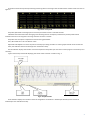
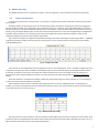
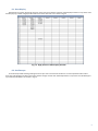
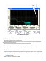
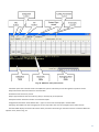
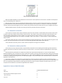
1
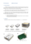
R Tech Electronics QMLab User Manual 1. QMLab Introduction QMLab software package is a multipurpose software instrument operating QMBox series devices. QMLab resolves a number of standard tasks common in automation of industrial objects and scientific laboratory equipment. This package is used with all QMBox series devices for configuration of given device and setting the parameters of required data acquisition and processing. QMLab software enables starting the operation immediately after connection of the device, because it does not require any additional programming or calibration. QMLab displays data in apropriate units of measurement through the number of digital and graphical visualisation options. The software’s QMParser utility converts data and saves it in standard text and binary formats compatible with the most of commonplace and specialized data imaging and processing programs (Excel, MathLAB, Cool Edit pro, PowerGraph, etc.) Starting from v.3.2.1., QMLab supports DAC devices. The software allows using DAC as a multichannel generator of sinusoidal signals, DC signals, as well as free shape signals by feeding user‐defined binary files of free length to DAC. QMLab software package is cost‐free and is supplied with all QMBox series devices. 2. QMLab Installation and Start‐up 2.1.
Requirements QMLab software runs on Windows XP or later version of 32‐bit Windows. Minimal hardware requirements: CPU ‐ 1GHz, RAM ‐ 1GB, hard disc ‐ 1GB of free space. 2.2.
Definitions QMBox hardware operated through QMLab software will be refferd to as Measuring System or System. Every QMBox consists of one or several same or different QMS modules, bundled in a single housing. We shall call every such unit (ADC QMS10, DAC QMS45, submodule carrier QMS301, etc.) Measuring Module or Module. Bundled and connected together they form Measuring Device or Device. Every module of the device can have up to 16 or 32 Measuring Channels or Channels, so the biggest, 8‐module device can have up to 256 channels. 2.3.
Installation To install the QMLab software package please run setup.exe file from QMLab software installation package folder and follow the instructions. 2.4.
Start‐up Before starting QMLab, the measuring device should be connected to the PC via USB port and switched on. QMLab can be launched with Start Menu (Start ‐> All Programs ‐> QMLab ‐> QMLab) or by running the QMLab.exe file from installed program folder (by default ‐ C:\Program Files\QMLab\ QMLab.exe). When started, QMLab first performs the initialization of measuring device, and then opens the main window. Depending on the quantity of modules in the device the start‐up process may take some time – from a few to a few dosen seconds. 3. QMLab Interface The main window of QMLab is shown on the Fig. 2 with controls and diplays listed below. 1 Fig 1. QMLab Main Window Start/Stop button is used to start/stop data acquisition session. Time Counter shows the time of current measurement in seconds, while Stop Time Box is used to set up required time of measurement in seconds. For more information on external starting, modules synchronization and setting measurement time, please refer to External starting, synchronization and time setting section. Close button is used for correct finishing of the work and closing QMLab. Visualization buttons start Osciloscope, Spectrometer and High Precision Data Display windows. For more information on data visualisation in external Osciloscope, Spectrometer and Data Display pop‐up windows please refer to Data Visualization section. Configuration table is used to set the values of measuring device parameters and the properties of data processing, visualization and saving during the anticipated data acquisition session. For more information on configuration, refer to Channels Configuration section. Configuration Parameter switch defines wich ‐ upper or lower limits are displayed in Cofiguration table. To Forget button is used to reset all values in the Configuration table to their default settings. When exiting the software, all the adjustments made during configuration stage, are saved in a special configuration file and restored when the software is restarted. If it is necessary to re‐set the default settings, this configuration file must be cleared by pressing To Forget button. Data Survey field displays similar to Configuration table digital chart representing real‐time measured parameters values in all active channels. Each cell holds five digits and symbols. If corresponding channel is inactive, the cell displays “‐‐‐‐‐“, when it is overloaded – “*****”. Normally working channel shows low precision (two digits after the decimal point) value of measured parameter in appointed units of measurement listed in the respective cell of Configuration table. 2 Screenshot of Data Survey field representing measuring device consisting of two modules with 4 and 8 channels is shown on Figure 2. Fig 2. Data Survey field Strip Chart field shows colored graphs of measured parameters values in selected channels. Indication Period switch sets data averaging and refreshing time for the display in Data Survey and Strip Chart fields. Indication Period can be assigned in the range from 0.2 second to 1 minute. Strip Chart has some picture adjustment and monitoring possibilities: Unit / Div switch sets Y‐axis unit division value. Shift slider and Shift box can move the picture vertically by scrolling the slider or entering required shift value into the box. Time / Div indicator shows time sweep (X‐axis unit division value). # Trace indicator displays the number of channels depicted in Strip Chart (current version of the program can handle up to 8 channels) Typical view of Strip Chart field displaying the charts of two channels is shown on Fig. 3. Fig 3. Strip Chart field # Osc indicator displays the number of channels assigned for visualisation in Osciloscope window (current version of Osciloscope has 4 available channels). 3 4. QMLab Operation The QMLab operation process includes three stages – system configuration, data acquisition and data post‐processing. 4.1.
System Configuration To prepare the system for the measurement it’s necessary to configure each channel of the device and set the time of the measurement. All the parameters of measuring channels and the properties of data visualization and saving are set to the Configuration table of the Main window. The Configuration table consists of 8 lines (max. number of measuring modules within one device) and 16 columns (max. number of measuring channels within one module), so each cell of the table corresponds to one channel. Initially, every cell displays default upper or lower limit of the parameter measured in this channel (depending on Configuration Parameter switch position) and its measuring units. During the configuration all the channels parameters can be set and changed according to the specific measurement requirements. Fig. 4 shows an example of Configuration table default settngs of the device consisting of 2 measuring modules – a QMS301 module (row 0) which includes 4 thermocouple channels (columns 0‐3) and 1 thermoresistor channel (column 14) and ADC module QMS10 (row 1): Fig. 4. Configuration table Each channel can be configured by left‐clicking with the mouse on corresponding cell. Then a contextual configuration menu is displayed. The upper part of the contextual menu displays similar to all the channels options for setting parameters of data processing, visualization and saving. In the lower part of the contextual menu, there are settings varying according to the particular type of the selected module and channel. For more information on these settings refer to Channels Configuration section. When the software is closed down all settings made during configuration stage are saved. Therefore, it is not necessary to re‐enter the values when the software is restarted. Data acquisition session, which is initiated by pressing Start button, can last for indefinite period, until Stop button is pressed. If it is necessary to define the exact period of data acquisition session, the required time (in seconds) must be entered in the Stop Time box as it’s shown on Fig. 4. Fig. 5. Measurment time setting During the process of data acquisition, the time elapsed from the beginning of the session is displayed in Time counter. Data acquisition session is stopped when Time counter value reaches the value set in Stop Time box. If the Stop Time value is set to ‐1, data acquisition session will continue until pressing Stop button. 4 The QMLab also has options of external starting and and synchronization of the measuring modules. How to prepare the system for external start and synchronize the modules is described in Common Options Configuration section. 4.2. Data Acquisition Data acquisition process consists of data collection from the sensors, pre‐processing, visualization and saving. Data collection starts by pressing Start button or by pre‐set external starting parameter. Obtained data is calibrated and converted to the required measuring units. If the type of the sensor connected to the channel is specified, the data can be standardized in compliance with the requirements of the particular type of sensor. For example, for thermocouple channels junction temperature compensation and transfer linearization calculations could be performed. QMLab also has few options of additional data processing ‐ it can calculate parameter’s RMS (quadratic mean) and slew rate (time derivate) of any measured parameter. For more information on data pre‐processing, refer to Common Options Configuration section. During data acquisition process, the collected, calibrated and converted to the required units of measurement data can be visualized. QMLab has two levels of data visualization – low precision data survey and high precision data visualisation. Low precision real‐time digital data from all the channels is displayed in the Data Survey field (Fig. 2). It also can be selectively depicted as graphic image in the Strip Chart field (Fig. 3). Both Data Survey and Strip Chart fields are embedded in the Main window of the program (Fig. 1). The selection of the parameters to be shown in the Strip Chart is described in Common Options Configuration section. QMLab has three pop‐up windows for high precision data visualisation. Data Display window is used for digital channel‐by‐
channel data indication. Graphic high precision visualization can be done by activating Oscyloscope or Spectrometer pop‐up windows. For more information on high precision data visualisation, refer to Data Visualization section. If needed, data can be saved in system’s own binary format on the computer hard disc. The selection of the parameters to be saved is described in Common Options Configuration section. 4.3. Data Post‐processing All the measurement data can be saved on the computer hard dics in system’s own binary format, but for further processing with specialized data imaging and processing programs (Excel, MathLAB, Cool Edit pro, PowerGraph, etc.) it should be converted into standard textual or binary wave format. For this task there’s separate QMParser utility included in the QMLab software package. More information on operating QMParser and data post‐processing canbe found in Data Conversion section. 5. Channels Configuration Each measuring channel of the system is configured by left‐clicking with the mouse on corresponding Cofiguration table cell. On click a contextual configuration menu is displayed. The upper part of the menu shows Common Options of data acquisition (Fig. 6). In the lower part of the contextual menu, there are Specific Options varying according to the particular type of the selected module and channel (Figs. 7&9). Situated in the middle of the contextual menu Configure Complete saves all channel settings in configuration file and closes the menu. Modified channel’s parameters are displayed in Configuration table and saved in system configuration file. On re‐start all parameters are restored from that file. To Forget button clears configuration file and system returns to default settings. Channel configuration parameters also can be changed throughout data acquisition process. But it should be noted, that only parameters set during initial configuration will be saved in configuration file, so the problems with post‐ processing of the data can occur. 5.1. Common Options The upper part of the contextual menu (Fig. 6) shows similar to all the channels options of data visualization, pre‐processing and saving. 5 Fig. 6. Common Options configuration menu Diagram Color opens color selector for colored marking of the data from configured channel. The curve of the respective parameter in the Strip Chart and the background of corresponding Configuration table cell will be shown in selected color. Diagram Enable checkbox allows graphic imaging of the data from configured channel. If Strip #1 checkbox is marked it’s displayed in the Strip Chart field (Fig. 3), if Oscilloscope & Spectrometer checkbox is marked – data from this channel is shown in Osciloscope and Spectrometer windows. Operation of high precision data visualisation is described in Data Visualization section. Data Saving Enable checkbox lets the user select if the data from configured channel should be saved on a hard disc. Display Units selector determins whether data will be shown in the units of measured parameter (Signal) or standardized and converted to the units of derivative parameter of selected type of sensor (Sensor). For example, in case of thermocouple channel measured parameter (Signal) units are milivolts (mV), while derivative parameter (Sensor) units are degrees of Celsium. Mean‐square Enable checkbox activates calculation and display of RMS (quadratic mean) of the measured parameter. Val/dt checkbox activates calculation and display of slew rate (time derivate) of the measured parameter. External Start checkbox sets external start mode of data acquisition session. In this mode, after pressing Start button, the system will wait for external start signal and data acquisition will begin only when such signal will be received. It can be used for multi‐module device synchronization – all marked channels will start working simultaneously after external start signal on any of them is received. The requirements for the external start signal are provided in the documentation of the measuring device. 5.2. Specific Options 5.2.1. QMS10 Module Configuration ADC module QMS10 by default is configured with 16 differential channels, all channels’ analog‐to‐digital conversion frequency 20 kHz and input range ‐10V…+10V. The user can modify all the parameters by left‐clicking on a corresponding cell of the configuration table and using contextual configuration menu. For the QMS10 lower part of the contextual menu appears as shown on Fig. 7. Fig. 7. QMS10 Specific Options configuration menu
6 Range selector switches measuring range to one of the preset values (±10 V, ±2.5 V, ±0.625 V, ±0.156 V). Channels setup function opens up sub‐menu shown in Fig. 8. Fig. 8. QMS10 module setup sub-menu Common Ground mode switches the module from the differential mode to common ground mode with up to 32 available common ground channels. Active Channels selector sets up the number of active channels of the module. ADC Frequency selector sets up analog‐to‐digital conversion frequency for all the channels of the module, which appears after confirmation as Rate in the main configuration menu (Fig. 7). 5.2.2. QMS301 Module Configuration QMS301 is carrier module for up to 16 S series submodules, which are single‐channel analog‐to‐digital converters for measurements with channel‐to‐channel galvanic isolation. Sampling rate on all channels is 250Hz. QMS301 can hold sensors for current (S20), voltage (S30), resistance (S50) or thermocouple (S40) and type of sensor should be selected from sub‐menu shown in Fig. 9. Fig. 9. QMS301 Specific Options configuration menu
Thermo Couple Type selector allows choosing a particular type of thermocouple (E, J, K, etc.) to select which type of sensor is connected to the channel. If there is a thermocouple working in Sensor mode and additional thermoresistor channel, temperature can be obtained with correction for cold junction compensation. 7 5.2.3. QMS45 Module Configuration Digital‐to‐analogue conversion module QMS45 can be used as multichannel generator of sinusoidal signals, the source of direct current or generator of free‐form unlimited duration signals generator (by convertion of user‐defined binary files). When QMS45 is present, QMBox Configuration table displays “DAC” in cells of corresponding to the module row. The contextual menu of QMS45 is shown in Fig. 10. Fig. 10. QMS45 channel setup menu Amplitude selector sets the amplitude of sinusoidal signal. Phase selector changes the phase shift of the channel. Frequency selector sets the frequency of the signal. If frequency is set to “0”, the channel will generate direct current. Play File button starts the search of pre‐defined binary .wav file. QMLab uses standard binary .wav files with special header, described in Appendix B of this Manual. The header has to be in 16‐bits format and the number of signals in file should not exceed 8, maximum number of channels in QMS45. The software automatically selects sampling frequency of user‐defined files. It’s possible to check it by opening contextual menu of working channel, which appears with that information as shown in Fig. 11. Fig. 11. QMS45 sample frequency checkout Sample rate displays sampling frequency selected by the software. 6. Data Visualization QMLab has three options for high precision data visualization – digital display, oscyloscope and spectrometer, stated with one of Visualization buttons. If graphical display (oscyloscope or spectrometer) is needed, the Oscilloscope&Spectrometer function should be activated in configuration menu of a corresponding channel.
8 6.1. Data Display Data Display is used for digital high‐precision channel‐by‐channel data indication. Data Display on button in top of the main window pops‐up a table of high‐precision data from all the channels as it’s shown in Fig.12. Fig. 12. High precision date display window 6.2. Oscilloscope An oscilloscope allows viewing oscillograms from up to 4 four channels of the device. It can be operated in two modes ‐ Auto Scan and Waiting Scan with the function of data storage on hard disk. Osciloscope button in top of the main window pops‐
up oscilloscope window as it’s shown in Fig. 13. 9 Fig. 13. Osciloscope window Controls of all four channels are located as under the oscilloscope’s display screen (Fig. 14) Fig. 14. Osciloscope channel control panel Channel information pane displays data about the source connected to this oscilloscope channel (number of the module and number of the channel in it, both counts starting with 0) and the Y‐axis devison value, which is set by Y‐axis scale setting selector. Offset selector regulates Y‐axis shift. It can be done with a knob or by sliding with the arrows or entering the value of the shift into the box below the knob. On the right from the oscilloscope display screen there are its common controls shown in Fig. 15. 10 Fig. 15. Osciloscope common controls Slope switch selects synchronization with positive or negative slope of the triggering signal. Trigger selector chooses the channel for synchronization or sets Auto regime without synchronization. Trigger level sets the triggering value of the synchronization parameter. It can be done with a knob or by sliding with the arrows or entering the value of the shift into the box below the knob. Time / Div selector chooses sweep time (X‐axis unit division value). Position selector sets X‐axis shift. It can be done with a knob or by sliding with the arrows or by entering the value of the shift into the box below the knob. Single button toggles the oscilloscope into waiting mode. The controls of this mode are shown in Fig. 16. 11 Fig. 16. Osciloscope waiting mode controls Start button activates waiting for a triggering signal. Save button saves the data from all active channels on the hard disc. NB! To save the data from the oscilloscope, standard data saving should be turned off (Data Saving Enable checkboxes on all channels common options menus has to be cleared). Buffer selector changes the size of the stored data buffer by sliding with the arrows or by entering the value in seconds into the box. NB! First half of the buffer is always reserved for background history data, what places the triggering event in the middle of the screen. Offset selector regulates X‐axis shift by sliding with the arrows or by entering the value of the shift into the box. 6.3. Spectrometer Spectrometer allows viewing spectrums from up to 4 four channels of the device. Spectrometer button in top of the main window pops‐up spectrometer window as it’s shown in Fig. 17. 12 Fig. 17. Spectrometer window Cursor is a point at the cross of the vertical and horizontal grids is used to define the coordinates of any point of spectrogram. The coordinates of spectrogram point are displayed under the spectrogram on the left. The cursor can be placed at any point of spectrogram by left‐click of the mouse. Every measuring channel has its own control pane, where: Hide checkbox allows excluding the channel from the picture. It can be used when several ranges are overlapping what aggravates visual perceiving of spectrogram. Reset FFT sum button starts accumulation of data for this channel from the beginning. Channel information shows spectrometer’s channel information: device module number, channel of the module number and the nymber of FFT points used for this channel. Max. FFT points’ slider is used to set the maximum number of points for spectrum calculation. 7. Data Conversion All the measurement data acquisited by the device can be saved on the computer hard dics in system’s own binary format, but for further processing with specialized data imaging and processing programs (Excel, MathLAB, Cool Edit pro, PowerGraph, etc.) it should be converted into standard textual or binary wave format. For this task there’s separate QMParser utility included in the QMLab software package. 7.1. QMParser utility QMParser utility’s main window is shown in Fig. 18. 13 Fig. 18. QMParser utility main window File button opens the initial file saved in the QMLab in system’s own binary format during data acquisition session. Output Dir button selects the folder for converted files. Go button starts conversion process. Output Type switch sets the format binary (.wav) or textual (.txt) for output files. # Samples counter shows the number of converted samples. Configuration Parameter switch defines wich ‐ upper or lower limits are displayed in Cannels table. Averaging Time slider sets data averaging time for the output file. Data can be averaged only for textual format. Channels table displays the initial information about processed. Left‐clicking on the table cell starts contextual Data Out Options menu, shown in Fig. 19. 14 Fig. 19. Data Out Options menu Data Out Enable checkbox includes the data from the channel to the output file. If the channel is included in the output file text in corresponding cell is underlined. Data Out Units selector determins whether data will be saved in the units of measured parameter (Signal) or standardized and converted to the units of derivative parameter of selected type of sensor (Sensor). For example, in case of thermocouple channel measured parameter (Signal) units are milivolts (mV), while derivative parameter (Sensor) units are degrees of Celsium. Val/dt checkbox activates calculation and saving of slew rate (time derivate) of the parameter. 7.2. Conversion to text files In Conversion to text files mode a separate textual (.txt) file for each channel is created. Names of those files consist of the number of measuring module and the number of the channel in this module. They contain information about the data in the form of symbolic representations of real numbers. The range and precision of the numbers can reach values up to 64‐bit standard PEX (type double) format. The numbers are placed in a file in one column, i.e. each character in a line is followed by CR/LF symbols. Information about channels is saved in special header files containing sampling rate, input range and measuring units of the channel. The names of those files are the same as of corresponding data files with header (.hdr) extension. In this mode the conversion process is rather slow and output files are larger than initial files. 7.3. Conversion to binary wave files In Conversion to binary wave files mode a separate wave (.wav) file for each sampling rate used during data acquisition is created. Some files may contain the data from only one channel, others – from many channels sampled with the same sample rate. Each output binary (.wav) file has a header that matches the requirements for RIFF files in a lay‐out corresponding to Windows PCM files (.wav). It enables using them as RIFF files for further processing with specialized data imaging and processing programs (Excel, MathLAB, Cool Edit pro, PowerGraph, etc.) A file created by QMParser contains information about the number of channels, sampling rate and type of the recorded data (integer or real). The example of such wave file header can be found in Appendix A of this Manual. Information needed to link information stored in RIFF file to measuring channels and their physical parameters which is absent from wave header is contained in a header text file (.hdr). The names of those files are the same as of corresponding data files. The requirements and limitations of the programs chosen for further analysis of the data should be kept in mind. The example of such header file can be found in Appendix B of this Manual. Appendix A. Format of WAV file header Field Length of the field in bytes 4 Total length of the field in bytes minus 8 4 ‘W’’A’’V’’E’ line 4 ‘fmt‘ line 4 ‘RIFF’ line 15 Length of the header (equals 16 plus length of extra information) 4 Data type (for QMLab must be = 1) 2 Number of channels 2 4 Sampling rate multiplied by the size of the sample in bytes 4 The total size of the sample (for all channels) in bytes 2 Size of the sample (for QMLab must be = 16) 2 Extra information (can be left unfilled) ‐‐ ‘data’ line Sampling rate in hertzes (Hz) 4 The size of data in bytes 4 Appendix B. Format of HDR file The example shows the output wave file for RIFF channel number 0 of the module channel 0 in module number 0. DD.MM.YYYY HH:MM:SS 12.02.2007 22:42:58 // time of start Fdscr 20000.0 // sampling rate Hardware Modul 0 // number of measuting module Hardware Channel 0 // number of channel in the module Wav File Channel 0 // number of channel in the RIFF file Minimum Value ‐10.0 // minimal measured value Maximum Value 10.0 // maximal measured value Unit V // units of measured parameter 16