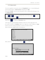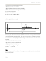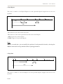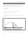
1
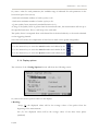
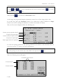
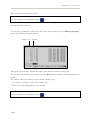
SYSCAL Pro – User’s manual
SYSCAL Pro
Standard & Switch (48 - 72 or 96) Version
10 channels Resistivity-meter for
Resistivity and IP measurements
User’s manual
June 2003
Terraplus USA Inc., 625 Valley Rd., Littleton, CO 80124
Phone: 303 799-4140 - Fax: 303 799-4776
E-mail: [email protected] - Web site: www.terraplus.com
SYSCAL Pro – User’s manual
CONTENTS
I. OVERVIEW.................................................................................................................... 3
I.1. GENERALITIES ............................................................................................................................... 3
I.2. DESCRIPTION.................................................................................................................................. 3
I.2.1. Front panel ....................................................................................................................................... 3
I.2.2. Backside ........................................................................................................................................... 4
I.2.3. Keyboard........................................................................................................................................... 4
I.2.4. Power supply ..................................................................................................................................... 6
II. IN-THE-FIELD............................................................................................................ 7
II.1. SET-UP ............................................................................................................................................... 7
II.1.1. Mode ............................................................................................................................................... 7
II.1.2. Name / Position ............................................................................................................................. 8
II.1.3. Stacking parameters......................................................................................................................... 9
II.1.4. Display options.............................................................................................................................. 10
II.1.5. Tx parameters ............................................................................................................................... 11
II.1.6. Electrode array .............................................................................................................................. 13
II.2. BEFORE ACQUISITION............................................................................................................ 14
II.2.1. Monitor ......................................................................................................................................... 14
II.2.2. Battery........................................................................................................................................... 14
II.3. ACQUISITION............................................................................................................................... 16
II.3.1. In-the-field implementation ............................................................................................................. 16
II.3.2. Standard mode............................................................................................................................... 16
II.3.3. Manual switch ............................................................................................................................... 22
II.3.4. Sequence creation............................................................................................................................ 23
II.3.4.1. Manual sequence............................................................................................................................................................................ 27
II.3.4.2. Automatic sequence...................................................................................................................................................................... 32
II.3.4.3. High speed ...................................................................................................................................................................................... 36
II.3.5. Continuous survey .......................................................................................................................... 39
II.3.6. Results during measurement ........................................................................................................... 41
II.4. AFTER ACQUISITION ............................................................................................................... 44
II.4.1. Result............................................................................................................................................ 44
II.4.2. Memory ......................................................................................................................................... 44
1/66
SYSCAL Pro – User’s manual
III. DATA MANAGEMENT ............................................................................................46
III.1. DATA DOWNLOAD.................................................................................................................. 46
III.2. DATA VISUALIZATION .......................................................................................................... 48
IV. OTHER FUNCTIONS...............................................................................................49
IV.1. FROM CONFIG MENU............................................................................................................. 49
IV.2. FROM TOOLS MENU................................................................................................................ 49
IV.2.1. Rs Check option .......................................................................................................................... 49
IV.2.2. Remote option.............................................................................................................................. 49
IV.3. FROM MEMORY MENU .......................................................................................................... 50
IV.3.1. Store option ................................................................................................................................. 50
IV.3.2. Store index option........................................................................................................................ 50
IV.3.3. Delete data option........................................................................................................................ 50
IV.3.4. Undelete data option .................................................................................................................... 50
IV.4. FROM SEQUENCE MENU...................................................................................................... 51
IV.4.1. Upload option.............................................................................................................................. 51
IV.4.2. Modify Config option ................................................................................................................... 51
IV.4.3. Delete option................................................................................................................................ 51
IV.4.4. Undelete option............................................................................................................................ 52
IV.5. FROM SYSTEM MENU ............................................................................................................. 52
IV.5.1. Clock .......................................................................................................................................... 52
IV.5.2. Check Switch option .................................................................................................................... 52
IV.5.3. Calibration option ....................................................................................................................... 52
IV.5.4. Format option.............................................................................................................................. 53
IV.5.5. Alarm options ............................................................................................................................. 53
V. FIRMWARE UPGRADE..............................................................................................54
ANNEX 1: EXTERNAL SWITCH PRO BOX ................................................................55
ANNEX 2: GEOMETRICAL PARAMETERS AND RESISTIVITY.............................56
ANNEX 3: IP PARAMETERS AND CHARGEABILITY ..............................................62
2/66
SYSCAL Pro – User’s manual
I. OVERVIEW
I.1. GENERALITIES
The SYSCAL Pro unit is a resistivity-meter designed for high productivity survey.
This all in one unit (containing transmitter – receiver and booster) is a very practical in-the-field
tool ; an external DC converter for an higher power can be added.
It allows to measure primary voltage and decay voltage curve values, giving thus resistivity and
chargeability (IP) data.
The main technical characteristics of this unit are the following ones:
- 10 reception dipoles available to carry out some measurements with high productivity in the
field
- 20 chargeability slices (automatic or user defined) able to measure the discharge phenomena
with an high accuracy
- a 1 µV resolution on the primary voltage allowing to obtain very accurate measurements
- a large graphic LCD screen allowing to visualize the data in real time either numerically or
graphically
The SYSCAL Pro unit can be also used in automatic switching mode (thanks to internal
switching board(s) or external Switch Pro box(es)) for intensive measurements in 2D and 3D.
I.2. DESCRIPTION
I.2.1. Front panel
The front panel shows the following features:
- Graphic LCD (128x140 dots) made of 16 lines by 40 characters
- Two plugs for current electrodes connection (?A? and ?B?) in Standard – Manual sequence Continuous survey or Manual switch mode (in Automatic sequence and High speed mode,
the electrodes are connected to switch cables plugged to the unit)
- Eleven plugs for potential electrodes connection (?1? to ?10? dipoles) in Standard - Manual
sequence - Continuous survey or mode (in Automatic sequence - Manual switch and High
speed mode, the electrodes are connected to switch cables plugged to the unit)
3/66
SYSCAL Pro – User’s manual
- Two plugs for internal battery chargers connection (?Charger? for Rx and Tx)
- Ventilation screw for possible going out of gas of the internal batteries during charge process
- ?+? and ?-? plugs for external battery connection
- Three pins plug (RS232 standard port) for the serial link cable connection (?Com 1?)
- Keyboard with 16 keys
- Switch On/Off
I.2.2. Backside
At the backside of the unit, the SYSCAL Pro has the following plugs:
- 1 serial link plug (?Com 2?) for external PC connection (useful in Continuous survey mode
where the ?Com 1? is used for a GPS connection) or for Switch Pro box connection
- 1 plug for a possible connection of a 1200 W AC/DC converter
- 1 plug for an external controlled DC converter
For the Switch version, some more plugs are present:
- 2 plugs for the connection of the switch cables
I.2.3. Keyboard
The keyboard of the SYSCAL Pro features some keys designed to be used either in the numeric
or in the function mode ; no confusion can be done between these modes, as the device knows
at any step of the use, in which mode it has to set itself.
The main functions of the SYSCAL Pro are reached either from these keys or from options of
the master menu.
• In the numeric mode, the meaning of the keys is obvious.
Each time one has to enter a numeric value, the available range for this value will be indicated in
the left bottom part of the screen
• In the function mode, the next table shows the description of these keys:
to transfer the data to the PC
to check the voltage level of the batteries
4/66
SYSCAL Pro – User’s manual
to check the reception voltage value without injection (ambient noise + Sp)
to select the operating mode and the injection parameters
to select the electrode array and the number of measuring channels
to check, before running a measurement, the grounding resistance value of the
electrodes
to visualize the results channel per channel (during and after measurement)
- to scroll up in a menu
- to go up in a range
- to change the result display
to visualize the results of the whole channels (during and after measurement)
- to move to the left in the menu bar
- to move to the left in the alphanumeric bar
- to move in the channel range
- to scroll down in a menu
- to go down in a range
- to change the result display
- to move to the right in the menu bar
- to move to the right in the alphanumeric bar
- to move in the channel range
- to stop the acquisition
- to reach the menu bar (at any step of the process)
to start the acquisition
- to stop the Rs check process
- to rub some letters or numbers
- to go out of any blocked function and go back to the menu bar
to validate an input or a selected function
5/66
SYSCAL Pro – User’s manual
I.2.4. Power supply
The SYSCAL Pro has to be supplied either by its 2 internal rechargeable batteries (12V – 7.2 Ah)
or by a 12V external battery (standard car battery) for the transmitter part.
• The internal batteries are located at the bottom part of the instrument. In case of the device
wouldn’t be used for a long time, it would be better to take out the battery in order to prevent
any possible leakage of this battery that could damage the casing.
Two specific chargers are supplied with the unit ; they have to be connected to the ?Charger?
plugs of the front panel.
Important note:
For security reasons, a ventilation screw is located on the front panel of the unit ; this component
allows to release a possible going out of gas of the internal batteries during the charge process in
case of defective or damaged batteries.
So, during the charge of the battery, the operator has to unscrew the ventilation screw, up to
release the small radial hole on the screw ; a retaining ring prevents the screw be totally removed
of the front panel.
The ventilation screw has to be locked while in-the-field using to ensure the watertightness of the
unit.
• In case of external battery use, it has to be connected to the ?+? and ?-? plugs of the front
panel, with the cables provided with the instrument.
Before using the SYSCAL Pro in the field, the first operation to do is to check the voltage level
of the batteries by the ?Tools|Battery? menu or by the
key (cf. II.2.2.).
The indicator located at the lower right part of the screen allows also to check the level of the
two batteries. This indicator is divided in two parts: the upper part is relative to the Tx
(transmitter) and the lower to the Rx (Receiver).
If an external battery is used for the current transmission, the battery level displayed will be
relative to the battery having the higher voltage value as the battery used will be always the one
having the highest level.
6/66
SYSCAL Pro – User’s manual
II. IN-THE-FIELD
II.1. SET-UP
To switch on the equipment, use the On/Off switch: the unit will display, during a while, the
type of the instrument, the version of the firmware and then, the following screen will appear,
with the menu bar:
Before performing an acquisition, one has first to introduce the set-up parameters ; all the
options relative to this set-up can be reached from the ?Config? menu and some of them,
directly from the keyboard.
II.1.1. Mode
The SYSCAL Pro unit allows to work in various operating modes.
The selection of the ?Config|Mode? menu will show the following screen:
7/66
SYSCAL Pro – User’s manual
From that window, one can see the current mode and one has the possibility to change it by the
?Change? button: the following modes are offered:
- Standard: standard use of the unit (without sequence creation): this mode requires the user to
enter the spacing parameters between each location.
- Manual sequence: Use of a sequence of measurement allowing to realize the acquisition
without introducing the spacing parameters between each location. In that mode, the spacing
parameters will be automatically computed and displayed between each location.
- Manual switch: Manual switching of electrodes. This mode requires the use of a Switch version
(or Switch Pro box(es))
Remark: this mode can be run for example for a monitor on specific electrodes or to re-start a
measurement on specific electrodes chosen by the user.
- Automatic sequence: use of a sequence of measurement allowing to switch automatically the
electrodes. This mode requires the use of a Switch version (or Switch Pro box(es)).
- High speed: Quick mode (pulse duration: 200 ms / 1 positive pulse and 1 negative pulse). This
mode requires the use of a Switch version (or Switch Pro box(es)).
Remark: this mode can be run for example to get a first idea of the resistivity values of the area.
Note:
In case of using the unit in Standard or in Manual switch mode, the set up parameters have to
be chosen from the various following options of the ?Config? menu.
For the other modes, requiring a sequence of measurement, the set up parameters have to be
specified while the sequence creation (cf. II.3.4.).
II.1.2. Name / Position
The selection of the ?Config|Name/Position? menu will display the following screen:
8/66
SYSCAL Pro – User’s manual
So, specify a filename in which the data will be stored (until one enter a new name, all the next
data will be stored with this filename).
One can specify also the location of the profile in longitude and latitude positions.
Procedure:
- For file name, use the
and
keys to move left and right the cursor in the
alphanumeric bar and press the
key each time the cursor is located below the letter you wish
to enter.
Then, locate the cursor below the ?↵? letter to validate the filename.
Automatically, the line New latitude will be created and highlighted at the bottom of the screen
- Use the numeric keys to enter the New latitude number and validate by the
key ; the
Latitude position will so be updated and the line New longitude will be automatically created
and highlighted
Use the numeric keys to enter the New longitude number and validate by the
key: the
longitude position will so be updated.
Note:
if a GPS is connected to the unit, instead of entering numerically the value, you’ll be able to press
the
key for a direct introduction of GPS data when New latitude and New longitude are
highlighted (any type of GPS using the NMEA 0183 norm can be used).
II.1.3. Stacking parameters
The selection of the ?Config|Stack/Q? menu will display the following screen:
Available range
9/66
SYSCAL Pro – User’s manual
So, enter a value for each parameter (the available range is indicated for each parameter in the
bottom left part of the screen):
- Stack min: minimum number of stacks (cycles) to do
- Stack max: maximum number of stacks (cycles) to do
- Q max: quality factor requested (standard deviation in %).
As long as the quality factor is greater than the introduced value, the measurement will run up to
the specified stack max. If not, it will stop to the stack min.
The quality factor is computed from each channel but is checked relatively to the results obtained
on the triggering channel.
Note that in IP mode, the computation of this factor is made on the global chargeability.
Procedure:
- Use the numeric keys to enter the min # number and validate by the
key
- Use the numeric keys to enter the max # number and validate by the
key
- Use the numeric keys to enter the Q max number and validate by the
key
II.1.4. Display options
The selection of the ?Config/Options? menu will show the following screen:
So, choose the various options relative to the display:
• Reading:
Average (X): the displayed values will be the average values of the pulses from the
beginning of the measurement.
Inst. (X): the displayed values will be the average values of the three latest pulses
(standard)
10/66
SYSCAL Pro – User’s manual
• Voltage:
Unsigned: the displayed average values of voltage will be absolute values (standard)
Signed: the voltage values will have a sign, which depends on the polarity of the measured
dipole voltage with respect to the first dipole voltage. Consequently, the resistivity values
will be also signed.
• IP values:
Raw: the displayed values will be the true partial chargeability values observed on the
decay curve (standard)
Normalized: the displayed values will be values normalized in regards to a reference decay
curve (not available for the Cole-Cole and Programmable modes) (cf. Annex 3 for more
information)
• Spacing unit:
Meter: the spacing values will be given in meters (standard)
Feet: the spacing values will be given in feet
Procedure:
Use for each option the
and
keys to move left and right the cursor and the
key to
validate the option you wish
II.1.5. Tx parameters
The selection of the ?Config|Tx parameters? menu or the
key will display the following
screen:
• Rho & Ip (resistivity and chargeability) or Rho (resistivity only) measurement
• Time: select the injection pulse duration: 250 ms - 500 ms - 1 s - 2 s - 4 s - 8 s.
11/66
SYSCAL Pro – User’s manual
• Mode (if Rho & Ip): choose the sampling of the partial chargeability slices
Arithmetic: arithmetic sampling with 3 to 20 partial chargeability slices
Semi logarithmic: semi logarithmic sampling with 3 to 20 partial chargeability slices
Logarithmic: logarithmic sampling with 2 to 6 partial chargeability slices
Cole-Cole: specific sampling used to calculate in a second time (from PROSYS software) the
Cole-Cole parameters.
Programmable: 20 fully programmable slices
• Vp or Vab requested: choose either:
- a constant injection value (Vab requested) and then select the value among [12V - 25V - 50V 100V - 200V - 400V - 800V - Max (1000V) - External DC] or
- a constant reception value (Vp requested) and then select the value among [Save energy (20
mV) - 50mV - 200mV - 800mV - Max (3V)]
Notes:
• The Vp value will be requested for the triggering channel (cf. II.1.6.). If the Vp value requested
induces overvoltage on channel 1, for example, the new channel for the Vp requested will be the
previous one, and so on until there’s no more overvoltage on channel 1.
• In switching configuration (use of switch cables), the Vab max will be 800V.
if Rho & Ip has been chosen, then, one will reach the IP parameters screen allowing to
visualize or to modify the values (in regards to the chosen IP mode):
Vdly: delay time (in ms) from which the samples (sampling rate: 10ms) will be taken into account
after injection, both for intensity and voltage measurements:
This delay time permits to be sure that all transient effects like IP and EM responses will be
vanished and so, won’t disturb the measurement.
12/66
SYSCAL Pro – User’s manual
Mdly: delay time (in ms) from which the voltage samples (sampling: 10ms) will be taken into
account after the current cut off.
Note:
The number of chargeability slices depends on the injection pulse duration previously chosen (cf.
Annex 3 for more information).
II.1.6. Electrode array
The selection of the ?Config|E. array? menu or the
key will display the following screen:
So, first, choose the electrode array you wish to use (cf. Annex. 2 for more information).
Then enter the number of channels to be used and the triggering channel
Note:
The triggering channel is the one that will be used for the voltage reception value requested (Vp
requested) ; this channel will be assigned of the character ?*? in the results displays in front of the
corresponding line.
Procedure:
For El. array: use the
k
and
keys to move up and down the cursor in the list and the
key to select the array you wish
For Nb channels and Trigger on: use the numeric keys and validate by the
key.
Note (cf Annex 2 for more information):
The maximum number of channels allowed is 10 except for the following arrays (1 channel max):
Pole-Pole - Wenner - Schlumberger.
So for these arrays, by default we’ll have Nb channel: 1 and Trigger on: 1
13/66
SYSCAL Pro – User’s manual
II.2. BEFORE ACQUISITION
Before running the acquisition, some tests have to be done to be sure that the measurement will
be performed in the best conditions:
II.2.1. Monitor
The selection of the
key (or the ?Tools|Monitor? menu) will show the following screen:
Graphic scale
Reception voltage curve
Channel number
Voltage value of the
displayed channel
This function allows to visualize in real time the reception voltage value and the corresponding
curve, channel per channel. This is just a monitoring of the reception voltages without injection
(Sp + ambient noise monitoring)
At this stage, you can change the graphic scale using the
be visualized by the
Press the
and
and
keys and the channel to
keys.
key to see the DC offset value (SP + noise): automatically, the Offset box will be
crossed and the voltage value will be indicated.
II.2.2. Battery
The voltage level of the batteries can be displayed by the
menu ; the following screen will appear:
14/66
key or by the ?Tools|Battery?
SYSCAL Pro – User’s manual
So, one can see the battery voltage value in V and the capacity (10 V means 0 % of capacity) for
the Tx (transmission) and the Rx (Reception) part.
Press a key to skip this function.
Note:
From the master screen, the indicator located at the lower right part allows also to have
continuously a view of the batteries level.
If one of the battery levels become too low, a warning message will appear after having pressed
the
15/66
key.
SYSCAL Pro – User’s manual
II.3. ACQUISITION
II.3.1. In-the-field implementation
The SYSCAL Pro can be used in various operating modes (cf. II.1.1.)
In regards to that mode, some actions have to be done before running the measurement.
In Standard (cf. II.3.2.) - Manual sequence (cf. II.3.4.1.) or in Continuous survey (cf. II.3.5.)
mode, the electrodes are directly connected to the front panel of the unit.
In Manual switch (cf. II.3.3.) - Automatic sequence (cf. II.3.4.2.) or High speed (cf. II.3.4.3.))
mode, the electrodes are connected to switch cables ; these cables are double ended, and so can
be reversed for a full flexibility (useful for the Roll along implementation)..
In that configuration, the SYSCAL Pro Switch unit is located at the centre of the configuration
(example given for the SYSCAL Pro Switch-48 unit):
1 2
23 24
25 26
47 48
SYSCAL Pro
Switch -48
The switch cables are supplied in several cable sections, in regards to the electrode spacing and
the number of electrodes, to keep a reasonable weight per reel.
II.3.2. Standard mode
Preliminary note:
The screens described below are relative to a Dipole-Dipole array with 5 meters between
electrodes and 6 channels of reception.
To run an acquisition in that mode, select the ?Config|Mode? menu ; a screen indicating the
current mode will appear: if Standard mode is displayed, press ?OK?.
If not, press ?Change? ; then the screen showing the various available modes will appear ; then,
select Standard mode.
16/66
SYSCAL Pro – User’s manual
Procedure:
Use the
and
keys to move up and down the cursor in the list and the
Standard, then press the
Then press the
key to select
key
key or select the ?Tools|Start? menu
At this stage, the program will display the batteries screen if one of the voltage levels is low.
So, in that case, press the ?Continue? button if you think that it will be sufficient or ?Stop?
button if you want to recharge the batteries or connect an external 12V battery.
Then, the first screen displayed will be the following one:
Position of the first injection electrode
Length of the injection dipole
Position of the first reception electrode
Length of the reception dipole
Shift to apply between the acquisitions
So, enter the spacing parameters (the spacing parameters are relative to the electrode array you
previously selected - cf. Annex 2 for more information):
Procedure:
For each spacing: use the numeric keys and validate each input by the
Then, the following screen will appear:
Coordinates of the electrodes
Current electrodes
Potential electrodes
17/66
key
SYSCAL Pro – User’s manual
Then, press the
key to run the acquisition.
The next screen is relative to the resistance measurement of the whole dipoles ; this allows to
check that all the electrodes are correctly connected ; if not, check the wires and try to improve
the contact with the ground.
The following example is given for an SYSCAL Pro used with 6 channels:
Note:
The value of the grounding resistance is displayed in kOhm.
If the line is open (electrode not correctly connected), the displayed value will be 999.999 kOhm
and the line will be highlighted ; one can press the
key to skip this value and to check the
next dipoles.
So, at the end of the test, press ?OK? button if the resistance values are correct ; until you don’t
press ?OK?, the Rs check test will be continuously performed ; so, if necessary, you can try in the
meantime to improve the grounding resistances.
Then, the measurement will start automatically with first, a filtering process:
Theoretical Injected voltage value
18/66
SYSCAL Pro – User’s manual
Note:
In the previous screen, the Tx value displayed is a theoretical value which can be sometimes
different from the actual value as a power or voltage limitation can occur.
Then, the results will be displayed in the following screen:
During the measurement, one has the opportunity to see various results and various type of
screens: cf § II.3.6. for more information.
At the end of the measurement, for the first acquisition, the program offers automatically to save
the data in the first memory area (?0?):
Available range of the memory area
Note that if you want to store the data from a specific memory area, use the numeric keys.
Then, press the
key to confirm.
If you don’t want to save the data (to check the results beforehand for example), press the
key ; you’ll have the possibility in a second time to store them, thanks to the ?Memory|Store?
menu.
19/66
SYSCAL Pro – User’s manual
Then to go on the profile, move your electrodes in the field, of the specified Move parameter (5
meters in our case) and so, press the
key.
If the data previously acquired has not been saved, a warning message will be displayed ; you’ll
have so the choice to go on the measurement (?Continue? button) or to stop it to store the
previous data (?Stop? button).
Then the next screen will be automatically displayed:
Then, from this window, choose the ?Move? button.
The following screen will be then displayed:
Note that all the electrodes have been shifted of 5 meters.
Then, press the
key to run the acquisition: the measurement will start automatically with the
same screen as previously.
Then, after acquisition of this second data set, the program offers for saving the data from the
next memory area (?6? in that case as the previously data have been stored in memory area from
?0? to ?5?):
20/66
SYSCAL Pro – User’s manual
Note that if you want to store the data from a specific memory area, use the numeric keys.
So, press the
key to confirm.
If you don’t want to save the data to check the results beforehand, press the
key ; you’ll
have the possibility in a second time to store them, thanks to the ?Memory|Store? menu.
Note:
If you want to store the data from a full memory area, the following warning message will be
displayed:
So, press ?Yes? to confirm, and ?Abort? to skip this function without overwriting the data.
If you press ?No?, the program will check automatically the first free memory area and will offer
to save the data from this one ; then, press
21/66
to validate.
SYSCAL Pro – User’s manual
II.3.3. Manual switch
To run an acquisition in that mode, select the ?Config|Mode? menu ; a screen indicating the
current mode will appear: if Manual switch is displayed, press ?OK?.
If not, press ?Change? ; then the screen showing the various available modes will appear ; then,
select Manual switch.
Procedure:
use the
and
keys to move up and down the cursor in the list and the
Manual switch, then press the
Then press the
key to select
key
key or select the ?Tools|Start? menu
At this stage, the program will display the batteries screen if one of the voltage levels is low.
So, in that case, press the ?Continue? button if you think that it will be sufficient or ?Stop?
button if you want to recharge the batteries or connect an external 12V battery.
Then, the first screen displayed will be the following one:
Then, enter the electrodes to be switched and press
22/66
key to validate:
SYSCAL Pro – User’s manual
Then, specify if an external switching box is used.
- No switch box (no switching capability: 10 channels standard using)
- Switch Pro (possibility to switch up to 10 channels (manually in that mode))
- Switch Plus / Multinode (extension boxes used to switch 1 channel (manually in that mode))
Then press the
key or select the ?Tools|Start? menu.
Then, one will reach exactly the same screens than in Standard mode (cf. II.3.2.), from which
we’ll have to specify the coordinates of the electrodes.
II.3.4. Sequence creation
For the other modes of measurement (Manual sequence - Automatic sequence and High
speed), before running the acquisition, one has first to create a sequence of measurement (i.e. a
list of quadripoles with the definition of the geometrical parameters) ; this has to be done by the
?Sequence|Creation? menu ; the following screen will appear:
Then, from this window, you have the opportunity to press the ?Wizard? button if you want to
create the sequence step-by-step, from the beginning.
If the set up parameters have been defined from the ?Config? menu, you can press directly the
?Default? button.
Press ?Abort? button to skip this function and reach the master menu
From the Wizard creation, you’ll reach successively the screen of the following Config
parameters:
- Name / Position (cf. II.1.2.)
23/66
SYSCAL Pro – User’s manual
- Tx parameters (cf. II.1.5.)
- Stacking parameters (cf. II.1.3.)
- Electrode array (cf. II.1.6.)
Note:
In ?Vp requested? mode, it would be judicious to choose a number of channels in relation
with the number of depth levels of the sequence.
For example, if 16 depth levels are programmed, a number of channels of 8 will allow to optimise
the measurement. Indeed, In that case, the unit will perform a first set of measurements of 8
channels and then another set of 8 channels: so, this will allow to get higher voltage levels in
reception than in the 10 channels configuration, as in that case a first set of measurements of 10
channels will be performed followed by a set of measurements of 6 channels).
Then, one will reach the geometry parameters screen:
From the ?Default? button of the Sequence creation screen, you’ll have only access to the
Filename screen and then you’ll reach directly the geometry parameters screen:
Then, enter the following parameters:
- min. spacing (a): minimum spacing between the electrodes (in meters)
- Depth level (lvl): number of levels of investigation (max:16)
- Nb of electrodes: total number of electrodes (linked to the length of the profile you wish to
explore and the spacing between electrodes)
- First electrode: first electrode to be used
- Position of the first electrode in X, Y coordinates
Then, the following screen will appear:
24/66
SYSCAL Pro – User’s manual
Choose Regular sequence to run a standard sequence and the Roll along seq. to run a roll
along sequence.
The selection of the Roll along seq. requires that you have previously entered the correct
spacing for the first electrode ; this spacing is given at the end of the creation of the regular
sequence (for the first roll along).
Indeed, at the end of the creation of a regular sequence, one will reach the following screen:
So, press ?Finish? to validate the sequence creation or ?Continue? if you want to modify the
sequence.
Notes:
• After creation of the sequence, the modification of the parameters from the options of the
?Config? menu will be taken into account.
• Up to 12 sequences can be stored into the SYSCAL Pro memory
25/66
SYSCAL Pro – User’s manual
Once the sequence has been created, it’s possible to visualize it from the ?Sequence|View?
menu: the list of sequences present in the memory will so be displayed:
Number of electrodes
So choose from this list, by the
validate by the
and
Number of measurement (quadripoles)
keys, the sequence you wish to visualize and
key: the following screen will appear:
# of the M electrode
# of the N electrode
# of the A electrode # of the B electrode
List of the quadripoles
of measurement
From this window, use the
and
keys to scroll up and down in the list and the
and
keys to visualize the set up parameters of the sequence.
Note:
From the SYSCAL Pro, one has the possibility to use also some sequences uploaded from the
sequence creation software, called ELECTRE II, in case of the sequences offered directly by the
SYSCAL Pro doesn’t match to your requirement (cf. IV.4.1.).
26/66
SYSCAL Pro – User’s manual
II.3.4.1. Manual sequence
In that process, after having created a sequence (cf. II.3.4.), one has to specify that the acquisition
has to be performed in Manual sequence mode.
Then select the ?Config|Mode? menu ; a screen indicating the current mode will appear ; so if
Manual sequence mode is selected, then press ?OK?.
If not, press ?Change?: a screen showing the three available modes will appear ; so, select the
Manual sequence mode.
Procedure:
use the
and
keys to move up and down the cursor in the list and the
select Manual sequence, then press the
key to
key
The list of sequences present in the memory will so be displayed:
So choose from this list, by the
the
27/66
and
key: the following screen appear:
keys, the sequence you wish to run and validate by
SYSCAL Pro – User’s manual
Then, specify if an external switching box is used.
- No switch box (no switching capability: 10 channels standard using)
- Switch Pro (possibility to switch up to 10 channels (manually in that mode))
- Switch Plus / Multinode (extension boxes used to switch 1 channel (manually in that mode))
Note:
As one can see from the previous screen, one has the possibility to work in that mode with
switch boards, but the main advantage is of course for a SYSCAL Pro standard version (no
switch boards).
Then press the
key or select the ?Tools|Start? menu.
The first screen will be relative to the filename, which you can change at this stage ; then press
the
key: the following screen will appear:
So, to start the measurement at the first quadripole, then press the
key (if you want to start
the measurement from another quadripole, enter its number and validate):
Then, the program will offer to store the resistance values of the dipoles:
28/66
SYSCAL Pro – User’s manual
So, if you choose ?Yes?, the standard Rs check process will be run and will indicate the resistance
of all the electrodes of the switch cable versus the reference electrode ?1? ; and, moreover, the Rs
check of the dipoles will be measured (between each set of measurements) and stored with the
measurements.
If ?No? has been selected, only the standard Rs check will be done.
Then, if you selected previously ?Yes?, during a while, a screen with the ?Rs check? message in
the lower left part of the screen, will appear.
Then, the next display will be:
Then, press the
key to run the acquisition.
During the measurement, one has the opportunity to see various results and various type of
screens: cf § II.3.6. for more information.
At the end the measurement, for the first acquisition, the program offers automatically to save
the data from the first memory area (?0?):
29/66
SYSCAL Pro – User’s manual
Available range of the memory area
Note that if you want to store the data from a specific memory area, use the numeric keys.
Then, press the
key to confirm.
If you don’t want to save the data (to check the results beforehand for example), press the
key ; you’ll have the possibility in a second time to store them, thanks to the ?Memory|Store?
menu.
Then the next screen will be automatically displayed:
Note that all the electrode positions have been shifted of 5 meters (as the min. spacing parameter
defined in the sequence is ?5? (cf. II.3.4.)). In Manual sequence mode, the unit computes
automatically the new spacing parameters ; so, you don’t have to use the ?Move? or the
?Modify? button between the acquisitions: then, one has just press the
key to continue the
sequence ; this is the advantage of that mode in regards to the Standard mode.
30/66
SYSCAL Pro – User’s manual
Then, after acquisition of this second data set, the program offers for saving the data from the
next memory area (?10? in that case as the previously data have been stored in memory area from
?0? to ?9?):
Note that if you want to store the data from a specific memory area, use the numeric keys.
So, press the
key to confirm.
If you don’t want to save the data to check the results beforehand, press the
key ; you’ll
have the possibility in a second time to store them, thanks to the ?Memory|Store? menu.
Note:
If you want to store the data from a full memory area, the following warning message will be
displayed:
So, press ?Yes? to confirm, and ?Abort? to skip this function without overwriting the data.
If you press ?No?, the program will check automatically the first free memory area and will offer
to save the data from this one ; then, press
31/66
to validate.
SYSCAL Pro – User’s manual
II.3.4.2. Automatic sequence
In that process, after having created a sequence (cf. II.3.4.), one has to specify that the acquisition
has to be performed in Automatic sequence mode.
Then select the ?Config|Mode? menu ; a screen indicating the current mode will appear ; so if
Automatic sequence mode is selected, then press ?OK?.
If not, press ?Change?: a screen showing the three available modes will appear ; so, select the
Automatic sequence mode.
Procedure:
use the
and
keys to move up and down the cursor in the list and the
select Automatic sequence, then press the
key to
key
The list of sequences present in the memory will so be displayed:
So choose from this list, by the
by the
and
key: the following screen appear:
Then, specify if an external switching box is used.
32/66
keys, the sequence you wish to run and validate
SYSCAL Pro – User’s manual
- No switch box (no switching capability: 10 channels standard using)
- Switch Pro (possibility to switch up to 10 channels (manually in that mode))
- Switch Plus / Multinode (extension boxes used to switch 1 channel (automatically in that
mode))
Then press the
key or select the ?Tools|Start? menu.
The first screen will be relative to the filename, which you can change at this stage ; then press
the
key: the following screen will appear:
So, to start the measurement at the first quadripole, then press the
key (if you want to start
the measurement from another quadripole, enter its number and validate):
Before running the measurement, for the first acquisition, the program offers automatically to
save the data from the first memory area (?0?):
Available range of the memory area
Note that if you want to store the data from a specific memory area, use the numeric keys.
Then, press the
33/66
key to confirm.
SYSCAL Pro – User’s manual
Note:
If you want to store the data from a full memory area, the following warning message will be
displayed:
So, press ?Yes? to confirm, and ?Abort? to skip this function without overwriting the data.
If you press ?No?, the program will check automatically the first free memory area and will offer
to save the data from this one ; then, press
to validate.
Then, after selection of the memory area, the program will offer to store the resistance values of
the dipoles:
So, if you choose ?Yes?, the standard Rs check process will be run and will indicate the resistance
of all the electrodes of the switch cable versus the reference electrode ?1? ; and, moreover, the Rs
check of the dipoles will be measured (between each set of measurements) and stored with the
measurements.
If ?No? has been selected, only the standard Rs check will be done:
34/66
SYSCAL Pro – User’s manual
Then, if you selected previously ?Yes?, during a while, a screen with the ?Rs check? message in
the lower left part of the screen, will appear during a time required for the measurement.
Then, the next display will be:
Quadripole number
Theoretical Injected voltage value
Note:
On that screen, the Tx value displayed is a theoretical value which can be sometimes different
from the actual value as a power or voltage limitation can occur.
The measurements will be then displayed.
The previous screen will appear between each set of measurements.
Note that during the measurement, one has the opportunity to see various results and various
type of screens (cf § II.3.6. for more information).
Notes:
• The estimated time left will be also displayed (in the upper right corner of the screen) after the
first set of measurements and between each set of measurements.
• To stop a sequence, press the
button ; if a sequence has not been stopped before the
end, a message (Sequence not ended…) will be displayed in the master screen
35/66
SYSCAL Pro – User’s manual
Then, if a start on the same sequence is run, the following screen will be displayed:
Then, press ?Continue? to continue the acquisition or press ?New? to run a new acquisition.
II.3.4.3. High speed
In that process, after having created a sequence (cf. II.3.4.), one has to specify that the acquisition
has to be performed in High speed mode.
Then select the ?Config|Mode? menu ; a screen indicating the current mode will appear ; so if
High speed mode is selected, then press ?OK?.
If not, press ?Change?: a screen showing the three available modes will appear ; so, select the
High speed mode.
Procedure:
use the
and
keys to move up and down the cursor in the list and the
select High speed, then press the
key to
key
Important note:
This mode uses by default the following parameters:
- Pulse duration: 200 ms
- Positive pulse followed by a negative pulse (In that mode, no IP measurements can be done).
Moreover, this mode requires to work with a constant value of injection. So, the sequence
has to be created with a Vab requested value or this can be modified from the Tx
parameters (cf. II.1.5.) before running the sequence.
After validation of the mode, the list of sequences present in the memory will so be displayed:
36/66
SYSCAL Pro – User’s manual
So choose from this list, by the
the
and
keys, the sequence you wish to run and validate by
key: the following screen appear:
Then, specify if an external switching box is used.
- No switch box (no switching capability: 10 channels standard using)
- Switch Pro (possibility to switch up to 10 channels (manually in that mode))
- Switch Plus / Multinode (extension boxes used to switch 1 channel (automatically in that
mode))
Then press the
key or select the ?Tools|Start? menu.
The first screen will be relative to the filename, which you can change at this stage ; then press
the
37/66
key: the following screen will appear:
SYSCAL Pro – User’s manual
So, to start the measurement at the first quadripole, then press the
key (if you want to start
the measurement from another quadripole, enter its number and validate):
Note:
After validation, if the type of injection is not based on a constant Vab value (?Vab requested?
mode), an error message will appear in a window. In that case, choose ?New? from this window
to reach directly the ?Tx Parameters? screen to modify the type of voltage requested (cf. II.I.5.).
Before running the measurement, for the first acquisition, the program offers automatically to
save the data from the first memory area (?0?):
Available range of the memory area
Note that if you want to store the data from a specific memory area, use the numeric keys.
Then, press the
key to confirm.
Note:
If you want to store the data from a full memory area, the following warning message will be
displayed:
So, press ?Yes? to confirm, and ?Abort? to skip this function without overwriting the data.
38/66
SYSCAL Pro – User’s manual
If you press ?No?, the program will check automatically the first free memory area and will offer
to save the data from this one ; then, press
to validate.
Then, the following screen will appear directly (no Rs check is performed in that mode):
Quadripole number
At the end of the sequence, we’ll reach automatically the master screen.
II.3.5. Continuous survey
This type of acquisition can be reached from the ?Tools|Continuous survey? menu.
This is a dynamic mode especially designed for marine acquisition.
In that mode, the SYSCAL Pro is in the standard mode configuration ; it means than we can use
simultaneously up to 10 reception channels. This corresponds to 10 levels of investigation in
Dipole-Dipole configuration.
In that mode, only resistivity measurements will be performed
After selection of that mode, one can specify if a GPS is connected to the unit:
Then, after validation, the following screen will appear:
39/66
SYSCAL Pro – User’s manual
Then, press ?OK? and the following screen will appear:
• In case of ?External computer? is selected, a waiting message (?Remote control?) will appear
; then, from a specific PC software, called SYSMAR, one has to define the position of the
electrodes, the pulse duration and the voltage value to inject ; then the measurement can be run.
The PC has to be connected to the other port (?Com 2? if ?Com 1? is used by the GPS).
At about every 2 seconds (minimum value), a measurement will be performed and stored
automatically in the PC. The GPS data are also continuously recorded and stored for a perfect
location of the profile.
Please refer to the on-line help file of SYSMAR software for more information.
• In case of the internal memory of the unit is used, one has first to define the following setup
parameters thanks to the options of the ?Config? menu:
- Name / Position (cf. II.1.2.)
- Tx parameters (cf. II.1.5.): specify the injection time and the Vab request.
Then after selection of ?Internal?, the following window will be displayed:
40/66
SYSCAL Pro – User’s manual
Then, specify the interval between measurements, in second, in the range [6 – 3600].
This value corresponds to the minimum step of measurement ; then validate: one will have then
to specify the first memory area from which the data will be stored ; after validation, if the type of
injection is not based on a constant Vab value (Vab requested), an error message will appear. In
that case, apply the modification from the ?Config|Tx parameters? menu and do anew the
procedure.
Note:
in case of no GPS is connected, the minimum value of the sample interval is: 1 s
II.3.6. Results during measurement
Whatever the operating mode (except for the High speed mode), the screens showing the
results will be the same:
The
key will show the results of the measurement, channel per channel whereas the
key will show the results of the measurement, for the whole channels.
• So, from the
41/66
key:
SYSCAL Pro – User’s manual
Resistivity Voltage received
(in
Ohm.m)
(in mV)
Channel number
Chargeability Quality factor
(in mV.V)
(in %)
Status bar
Running stack
Injection pulse duration
Battery status (Tx/Rx)
R: Rho mode
M: Rho & IP (Raw values) mode
N: Rho & IP (Normalized values) mode
Running of the measurement
X : average value
X : instantaneous value
During the measurement, one can use the
- Pressing the
and
Stack min
Stack max
keys to change the displays:
key will allow to see the current value (in mA) instead of the chargeability
(Mp) value.
- Pressing the
key one more time will allow to see the Sp value (Self potential in mV)
instead of the current value
- Pressing the
key one more time will allow to check if there are some overload in
reception
The overload thresholds are the following ones:
VP1-P2: 15 V and
? VPi-Pi+1: 15 V
i=2
- And then, pressing the
channel of measurement.
42/66
key one more will allow to see the decay curves for the whole
SYSCAL Pro – User’s manual
- Press the
• And from the
one more time to come back to the first screen.
key:
Grounding resistance (in kOhm)
# Channel
Status bar
During the measurement, one can use the
and
keys to see the results channel per
channel.
At this stage, you can use also the
key to visualize the partial chargeability values of the
current channel.
- Pressing the
- Press the
key one more time will allow to visualize the spacing parameters
key one more time to visualize the location of the profile (longitude and latitude
position)
- Press the
key one more time to come back to the first screen.
Note:
The parameters displayed during the acquisition depends on the injection pulse duration
selected. Indeed, if a low injection time has been selected (250 ms for example), only
resistivity values will be displayed.
43/66
SYSCAL Pro – User’s manual
II.4. AFTER ACQUISITION
II.4.1. Result
Once a measurement has been performed, the results can be visualized, in the same way than
during the measurement, by the
The
or by the
key.
key will show the results of the previous measurement, channel per channel.
This function can also be reached from the ?Tools|Result? menu.
The
key will show the results of the previous measurement, for the whole channels.
The screens will be exactly the same that the ones shown during the measurement and you’ll have
the same functions offered (cf. II.3.6.).
Note:
This function is mainly useful for the Standard mode. Indeed, in the modes where a
sequence of measurement is run automatically, we’ll only have a view of the last
measurement ; and for a standard sequence, this corresponds to a measurement
performed only on the channel 1.
II.4.2. Memory
The memory size of the unit is 21018 data points.
One has the opportunity to recall a data point previously stored into the memory of the unit.
Each data point is stored in a memory area.
To do that, select the ?Memory|Recall? menu: the following screen will appear:
44/66
SYSCAL Pro – User’s manual
Then select the memory area you wish.
Procedure:
Use the numeric keys and validate by the
key
The screens will be exactly the same that the ones shown during the measurement and you’ll have
the same functions offered.
You can also visualized the whole data files stored in the memory by the ?Memory|Explore?
menu: the following screen will appear:
Memory area Attribute
This option allows only to visualize the name of the data files with the storage date:
You can enter the memory area number you wish (List # area) in order to scroll up and down in
the list.
The attribute (A) of the memory area can be the following one:
- ? ?: if a data is currently stored in that memory area
- ?D?: if the corresponding data has been deleted
Procedure:
Use the numeric keys and validate by the
45/66
key
SYSCAL Pro – User’s manual
III. DATA MANAGEMENT
Once the measurement has been performed and the data stored in the internal memory of the
unit, one can download the data to the PC, connected to the ?Com 1? plug.
This has to be done by the PROSYS software.
PROSYS software is the data visualization, processing and export software for all the SYSCAL /
ELREC type units of IRIS Instruments.
So, after having installed PROSYS software in the PC (by the ?SYSCAL Utilities? CD-ROM
supplied with the unit), run the ?Prosys.exe? file from the installation directory.
Note:
PROSYS software has an on-line help file, which will help you in the various tasks.
III.1. DATA DOWNLOAD
From
PROSYS
software,
select
the
?Communication|Data
download|SYSCAL
Pro/ELREC Pro? menu ; the following screen will appear:
So, you’ll have the choice to select either the first and last data points to transfer (?First #? and
?Last #?) or to enter the name of a file, to download the whole data stored with this file name
(?Specific filename? area) ; note that you can enter a ? *? to download the whole memory.
46/66
SYSCAL Pro – User’s manual
Notes:
• The ?High speed Download? box permits to transfer the data at 115 200 bauds.
• You can choose also to delete data after download crossing the appropriate box
• Up to 16000 data points can be managed by PROSYS software. So, if more data points are
present in the memory of the unit, you’ll have to transfer the data in several times.
Then, click on the ?Download? button: the following screen will appear:
Then, press the
key (or select the ?Memory|Data download? menu) from the SYSCAL
Pro: the data transfer will start ; a bar graph showing the transfer progress will appear in the
PROSYS window.
After data transfer, PROSYS offers to save the data with a filename ; the extension of these files
is ?bin?.
47/66
SYSCAL Pro – User’s manual
III.2. DATA VISUALIZATION
Once a data file has been transferred, one can visualize it thanks to the ?File|Open? menu.
Then select the ?.bin? file you wish to open ; the following screen will appear:
Then, from the master menu, you’ll be able to visualize graphically the results, process (filtering topography insertion,…) the data and create some export files for the commonly used
interpretation software.
For more information, please refer to the on-line help file of PROSYS software.
48/66
SYSCAL Pro – User’s manual
IV. OTHER FUNCTIONS
IV.1. FROM CONFIG MENU
The Load default option allows to load the default set-up parameters.
IV.2. FROM TOOLS MENU
IV.2.1. Rs Check option
The Rs Check option allows to run a grounding resistance measurement for the dipoles.
The screen is the same that the first one appearing after having pressed the
key:
- In Standard - Manual sequence and Manual Switch modes, the screen displays the result for
the injection and the reception dipoles.
- In the Automatic sequence and High speed modes, the screen displays the result for the
electrodes of the sequence versus the reference electrode ?1?.
Notes:
• In High speed mode, this option is particularly useful as no Rs check process is performed
before running the measurement
• In Automatic sequence and High speed modes, the Rs check process can be stopped by the
button.
IV.2.2. Remote option
This option allows to use the system in the following ways:
• Connect a modem to the ?Com 1? of the unit to be able, remotely, to upload a sequence from
the ELECTRE II software and download the data from the PROSYS software.
For more information, please refer to the on-line help file of ELECTRE II and PROSYS software.
• Or, connect a PC directly to the unit (?Com 1?) to drive it from a specific PC software.
49/66
SYSCAL Pro – User’s manual
IV.3. FROM MEMORY MENU
IV.3.1. Store option
After a measurement, one has the choice to store the data directly or not.
If you choose not to store to data (to check them beforewards for example), you’ll have in a
second time the opportunity to store them thanks to the ?Memory|Store? menu.
IV.3.2. Store index option
This option allows to select a memory area from which the next measurements will be stored.
This option is useful if you programmed a wake up of the unit (thanks to the ?Alarm? options of
the ?System? menu (cf. IV.5.5.).
IV.3.3. Delete data option
This option allows to delete some data from the internal memory ; one has just to specify the
block to erase (first and last data point to erase) ; a message will ask you to confirm the delete.
IV.3.4. Undelete data option
This option allows to undelete 1 datum point that have been previously deleted. So, this means
that if some data have been deleted, you’ll have the opportunity to retrieve these data. To do that,
you’ll have to enter the area number of the data point ; a message will indicate if the undelete
process was successful or not.
Note:
This can be done only if you didn’t write into this memory location in the meantime.
50/66
SYSCAL Pro – User’s manual
IV.4. FROM SEQUENCE MENU
IV.4.1. Upload option
This option allows to load a sequence created from ELECTRE II software if you need to run a
specific sequence of measurements. Selecting this option, a waiting message will appear on the
screen ; then, upload the sequence from the software.
The advantages of ELECTRE II software is that you can create any type of sequence of
measurements and particularly 3D or borehole sequences .
For more information, please refer to the on-line help file of ELECTRE II software.
IV.4.2. Modify Config option
This option allows to modify some parameters of a sequence:
So, first select in the list the sequence you wish to modify and then, you’ll have access to the
following parameters:
- Tx parameters (cf. II.1.5)
- Electrode array (cf. II.1.6)
IV.4.3. Delete option
This option allows to delete one (?One? button) or the whole sequences (?All? button) stored in
the SYSCAL Pro memory.
If you choose ?One?, you’ll have then to select from the list the sequence you wish to erase.
If you choose ?All?, a message will ask you to confirm the delete.
Press ?Abort? to skip this function and reach the master menu
51/66
SYSCAL Pro – User’s manual
IV.4.4. Undelete option
This option allows to undelete a sequence previously deleted. So, this means that if some
sequences have been deleted, you’ll have the opportunity to retrieve these sequences. To do that,
you’ll have to enter the # of the deleted sequence ; a message will indicate if the undelete process
was successful or not.
Note:
This can be done only if you didn’t create any sequence in the meantime.
IV.5. FROM SYSTEM MENU
IV.5.1. Clock
This option allows to program the internal clock of the unit ; the date/time are stored into the
memory.
IV.5.2. Check Switch option
This option allows to test the switching of 1 specific electrode.
So, one has just to specify the electrode to be switched and create a short circuit between this
electrode and the P2 electrode. Then a resistance measurement (given in kOhm) will be
performed.
IV.5.3. Calibration option
This option allows to run the calibration of the whole channels.
This has to be done after firmware upgrade and also if you have a doubt about the received
voltage levels.
This operation has to be performed without connected dipoles.
After having chosen this option, the following screen will appear:
52/66
SYSCAL Pro – User’s manual
The result of the latest calibration is so displayed ; to perform a new one, press ?New? button.
The results have to be the following ones:
Sc < 1.00 and Of < 2.30 for the whole channels.
Press the ?Exit? button to skip this option.
IV.5.4. Format option
This option will re-initialize the unit ; so, all the data and sequences will be lost if you perform
this operation ; a message will ask you to confirm the format.
IV.5.5. Alarm options
This option has to be used to program a wake up of the unit.
This allows to specify the time (hour/minutes) of the wake up (2 wake up can be programmed in
the unit (?Set Alarm 1? - ?Set Alarm 2? options)).
After that, the ? Start Alarm? option has to be used: the following screen will appear:
Then, make you selection by the arrow keys and validate by the
53/66
key
SYSCAL Pro – User’s manual
V. FIRMWARE UPGRADE
The SYSCAL Pro unit is programmed in flash ROM.
To upgrade it, an ?e-Flash? programmer is supplied with the unit.
This programmer has to be used to upgrade the firmware of the reception (Rx) and the
transmitter (Tx) boards.
A specific PC software, called E-FLASH, has to be used to perform this process.
Note:
Before performing the upgrade, transfer the whole measurements to a PC.
Indeed, depending of the upgrade version, the memory will be totally erased.
So, after having installed E-FLASH software in the PC (thanks to the ?SYSCAL Utilities? CDROM supplied with the unit), run the ?eFlash.exe? file from the installation directory.
For more information, please refer to the on-line help file of E-FLASH software.
After firmware upgrading, we advise to run a calibration of the system (by the
?System|Calibration? menu (cf. IV.5.3.).
54/66
SYSCAL Pro – User’s manual
ANNEX 1: EXTERNAL SWITCH PRO BOX
To perform 3D acquisition keeping the capability to use 10 reception channels in switching
mode, an external switching box, called Switch Pro has been developed.
This external box can be connected to the SYSCAL Pro unit (Standard or Switch version), by a
specific cable connected between the ?Com 2? plug of the SYSCAL Pro and the ?LINK IN?
plug of the Switch Pro).
This box can be used to drive 48, 72 or 96 electrodes ; to extend the number of electrodes
several boxes can be connected by specific cables connected between the ?LINK OUT? plug of
the previous Switch Pro box to the ?LINK IN? plug of the next Switch Pro box.
The following scheme shows the in-the-field configuration of the electrodes of a SYSCAL Pro
Switch-48 unit with a Switch-48 Pro box:
49
72
73
96
Switch Pro 49-96
LINK IN
1
24
25
48
COM 2
SYSCAL Pro
Switch -48
On the Switch Pro box, a display with two keys (?MENU? - ?CHANGE?) allows to choose the
numbering of the electrodes to make it compatible with your SYSCAL Pro unit.
The ?MENU? key allows to reach the ?increment node function?: then by the ?CHANGE?
button, choose the numbering. Press the ?MENU? key to reach the ?decrement node function?.
Then, press anew the ?MENU? key to see the type of Switch box (Pro in standard) ; you can
change it by a Switch Plus box (1 channel switching) to be compatible with a SYSCAL Switch unit.
Note:
The Switch Pro box has an internal rechargeable 12V – 7 Ah battery. As for the SYSCAL Pro, for
security reasons, a ventilation screw is located on the front panel of the Switch Pro box (cf. I.2.4.).
An external 12V standard car battery can be connected to the front panel (?+? and ?-? plugs
(Input 12 V)). If the battery level becomes insufficient (lower then 9.6 V), a ?Low Batt? message
will appear on the screen and a ?Switch Error? message will appear on the SYSCAL Pro.
55/66
SYSCAL Pro – User’s manual
ANNEX 2: GEOMETRICAL PARAMETERS AND RESISTIVITY
The methods for measuring the subsurface resistivity by DC current injection are all based on the
same principle:
• a current is sent in the ground through two electrodes (A, B - electrodes connected to the
transmitter).
• the current creates an equipotential distribution making it possible to measure a potential
difference between two other electrodes, which are potential ones (some arrays allowing to drive
simultaneously up to ten potential dipoles (P1, P2…P10,P11)).
• an apparent resistivity is then defined by: Ro = K.V/I where K (geometric factor) only
depends on the geometric array of the electrodes in the field and is expressed by:
For the dipole i: Ki = 2π / |1/APi - 1/APi+1 - 1/BPi + 1/BPi+1|
The various configurations only differ by the position of the electrodes with K assuming a more
specific expression.
In regards to the chosen electrode array (
key), one will have several specific parameters to
enter:
Electrode array
Geometrical parameters to specify
Max. number of dipoles
Dipole-Dipole
XCA
A-B
XP1
10
Pole-Dipole
XCA
XP1
P1-P2
10
Pole-Pole
XCA
XP1
1
Wenner
Mid
AB/3
1
Schlum
Mid
AB/2
MN/2
Grad. rctgl
XCA
A-B
XP1
P1-P2
10
Poly-Dipole
XCA
A-B
XP1
P1-P2
10
Poly-Pole
XCA
XP1
P1-P2
56/66
1
10
SYSCAL Pro – User’s manual
Remark:
In the following pictures, the X axis is defined as the AB axis, the Y axis is directly perpendicular
to AB and the origin 0 is taken as any arbitrary point.
• Dipole-Dipole
A-B
0
A
A-B
B
P1
P2
P3
X
1.1.1.1.1.1
XCA
XP1
- XCA: abscissa of the first current electrode
- XP1: abscissa of the nearest potential electrode from the AB dipole
- A-B: length of dipoles (current and potential):
|AB| = |P1 P2| = … = |P10 P11|
By setting niD as the distance between the midpoints of the dipoles AB and PiPi+1, we have:
Ki = π niD (ni2- 1)
• Pole-Dipole
P1-P2
0
A
B(∞)
P1
1.1.1.1.1.3
P2
P3
X
1.1.1.1.1.2
XCA
XP1
The current electrode B has to be placed sufficiently far from the other electrodes to be able to
ignore 1/BPi (generally 5 times the maximum distance between A and M)
- XCA: abscissa of the first current electrode
- XP1: abscissa of the nearest potential electrode from the AB dipole
- P1-P2: length of the potential dipoles:
|P1 P2| = … = |P10 P11|
Ki = 2π / (1/APi – 1/APi+1)
57/66
SYSCAL Pro – User’s manual
• Pole-Pole
In this array, the electrodes B and N have to be set sufficiently far from the A and M to be able
to ignore 1/BM, 1/BN and 1/AN (generally 10 times the maximum distance between A and M)
B(∞)
A
M
N(∞)
0
X
XCA
XP1
- XCA: abscissa of the current electrode
- XP1: abscissa of the potential electrode
K = 2π / (1/AM)
• Wenner
0
A
M
N
B
X
Mid
AB/3
- Mid: abscissa of the centre of MN
- AB/3: a third of the distance between the current electrodes
So K remains constant all along the profile axis.
• Schlumberger
0
A
M
Mid
MN/2
AB/2
58/66
N
B
X
SYSCAL Pro – User’s manual
The electrodes keep constant relative positions.
- Mid: abscissa of the centre of MN
- AB/2: half-distance between the current electrodes.
- MN/2: half-distance between the potential electrodes.
K is a constant of the profile:
If AB/2 = a and MN/2 = b
2
2
K = π (a - b ) / 2b (if AB/2 > MN/2).
• Grad. rctgl (Gradient rectangle)
Y
P1-P2
1.1.1.1.1.4
P1
0
A
XCA
P2
P3
1.1.1.1.1.5
B
X
XP1
AB
In this array, the AB electrodes are fixed and the Pi electrodes are moved parallel to AB inside
a zone located in the central part of AB. This array serves to observe variations in resistivity
on a surface for a relatively high investigation depth without the need to move the current
electrodes.
- XCA: abscissa of the first current electrode
- XP1: abscissa of the first potential electrode
- A-B: length of the current dipole
- P1-P2: length of the potential dipoles
|P1 P2| = … = |P10 P11|
Note:
In that configuration, the Y coordinate of the reception electrodes (Pi) can be introduced directly
from the SYSCAL Pro.
59/66
SYSCAL Pro – User’s manual
• Poly-Dipole
This array is similar to the Dipole-Dipole one with potential dipoles lengths that can be user
specified.
0
A
B
P1
XCA
P2
P3
1.1.1.1.1.6
X
P1-P2
A-B
XP1
- XCA: abscissa of the first current electrode
- XP1: abscissa of the nearest potential electrode from the AB dipole
- A-B: length of the current dipole
- P1-P2: length of the potential dipoles
Note:
And, in a second time, you can modify the position of each potential electrode, selecting the
?Move? button after having introduced these spacing parameters.
• Poly-Pole
0
A
B(∞)
P1
P2
X
P3
1.1.1.1.1.7
XCA
P1-P2
XP1
This array is similar to the Pole-Dipole one with potential dipoles lengths that can be user
specified.
60/66
SYSCAL Pro – User’s manual
The current electrode B has to be placed sufficiently far to be able to ignore 1/BPi
- XCA: abscissa of the current electrode
- XP1: abscissa of the nearest potential electrode from the AB dipole
- P1-P2: length of the potential dipoles
Note:
And, in a second time, you can modify the position of each potential electrode, selecting the
?Move? button after having introduced these spacing parameters.
Ki = 2π / (1/APi – 1/APi+1)
61/66
SYSCAL Pro – User’s manual
ANNEX 3: IP PARAMETERS AND CHARGEABILITY
The partial chargeabilities measurements (Mi) and the average global one deduced (Mg) give some
information regarding the ability of the soil to charge itself due to a current flow.
The partial chargeability of the window ?i? is measured thanks to the following formula:
Mi = ∫ Vdt / TMi.VMN
TMi
And the global chargeability is computed thanks to the following formula:
n
n
Mg = ∑ (Mi.TMi) / ∑ TMi
i=1
(n: number of IP windows)
i=1
The discharge phenomena observed during the relaxation time can be described according to the
following curve:
Voltage (mV)
VMN
M1
M2
M3
Time (ms)
Vdly
Mdly TM1
Current injection time
Relaxation time
With the SYSCAL Pro, up to 20 IP windows can be used to define the decay curve.
62/66
SYSCAL Pro – User’s manual
The number of IP windows available for the measurement depends on the type of IP mode and
on the current injection time:
⇒ Current injection times available (cf. II.1.4): 500 ms - 1 s - 2 s - 4 s - 8 s
⇒ Types of IP mode available (cf. II.1.4): Arithmetic – Semi logarithmic – Logarithmic
Cole-Cole - Programmable
For a given current injection time and IP mode, the program will choose automatically the IP
parameters (Mdly, Vdly, TMi) that will be used for the measurement.
Note:
The programmable mode is a mode where 20 fully programmable windows are available. The
operator has to select the delay time (Mdly) with a minimum of 20 ms and the width of each
partial window (TMi) with a minimum of 10 ms. Vdly is automatically determined by the injection
time chosen.
In the following tables, the preset TMi values are given for each IP mode (1 means TM1 …):
• Time = 500 ms
Mode Vdly Mdly 211
2
3
4
5
6
7
8
9
10
11
12
13
14
15
16
17
18
19
20
Arith.
280
60
40
40
40
0
0
0
0
0
0
0
0
0
0
0
0
0
0
0
0
0
Semi
280
40
40
80
160
0
0
0
0
0
0
0
0
0
0
0
0
0
0
0
0
0
Log.
280
160
80
180
0
0
0
0
0
0
0
0
0
0
0
0
0
0
0
0
0
0
Cole
280
160
80
180
0
0
0
0
0
0
0
0
0
0
0
0
0
0
0
0
0
0
• Time = 1000 ms
Mode Vdly Mdly 211
2
3
4
5
6
7
8
9
10
11
12
13
14
15
16
17
18
19
20
Arith.
580
120
40
40
40
40
40
40
40
40
40
40
40
40
40
40
40
40
40
40
40
40
Semi
580
40
20
20
20
20
20
20
20
20
40
40
40
40
40
40
80
80
80
80
80
80
Log.
580
160
120 220 420
0
0
0
0
0
0
0
0
0
0
0
0
0
0
0
0
0
Cole
580
20
10
20
20
20
20
30
30
30
40
40
40
50
50
50
60
60
70
80
90
20
• Time = 2000 ms
Mode Vdly Mdly
1
2
3
4
5
6
7
8
9
10
11
12
13
14
15
16
17
18
19
20
Arith.
1260
240
80
80
80
80
80
80
80
80
80
80
80
80
80
80
80
80
80
80
80
80
Semi
1260
40
40
40
40
40
40
40
80
80
80
80
80
80
80
160 160 160 160 160 160 160
Log.
1260
160
120 220 420 820
0
0
0
0
0
0
0
0
0
Cole
1260
20
20
40
40
50
60
70
80
90
63/66
30
30
30
0
0
0
0
0
0
0
100 110 120 130 140 150 160 180 200
SYSCAL Pro – User’s manual
• Time = 4000 ms
Mode Vdly Mdly 211
2
3
4
5
6
7
8
9
10
11
12
13
14
15
16
17
18
19
20
Arith.
2620
480
160 160 160 160
160
160 160 160 160 160 160 160 160 160 160 160 160 160 160 160
Semi
2620
160
80
80
80
80
80
Log.
2620
160
120 220 420 820 1620
0
0
0
Cole
2620
20
40
90
100 110 120 140 160 180 200 220 250 280 320 380 450 530
5
6
7
80
80
50
60
80
70
80
160 160 160 160 160 160 320 320 320 320 320 320
0
0
0
0
0
0
0
0
0
0
0
0
• Time = 8000 ms
Mode Vdly Mdly 211
2
3
4
8
9
10
11
12
13
14
15
16
17
18
19
20
Arith.
5340
960
320
320 320 320
320
320
320 320 320 320 320
320 320 320 320 320 320 320
320
320
Semi
5340
320
160 160 160 160
160
160
160 160 320 320 320
320 320 320 640 640 640 640
640
640
Log.
5340
160
120 220 420 820 1620 3220
0
0
Cole
5340
20
40
60
80
100
120
150
0
0
0
0
0
0
0
0
0
0
0
0
180 220 250 280 320 360 400 450 500 580 700 850 1010 1180
About the IP values type, note that the changing ?raw (R) ⇔ normalised (N)? can be realised
after the acquisition.
The normalization allows to homogenize the data that have been obtained with various injection
and integration times. This is made with respect to a standard decay curve, which is the one
obtained with the following parameters:
Mode:
Logarithmic
Injection time: 2000 ms
Vdly:
1260 ms
Mdly:
160 ms
TM1:
120 ms
TM2:
220 ms
TM3:
420 ms
TM4:
820 ms
The coefficients to multiply, allowing to go from a type to the other one, are indicated in the
following tables:
64/66
SYSCAL Pro – User’s manual
500 ms
Arithmetic
Semi logarithmic
Logarithmic
R→N
N→R
R→N
N→R
R→N
N→R
Mg
0.72
1.39
Mg
0.94
1.06
Mg
1.32
0.76
M1
0.60
1.67
M1
0.55
1.81
M1
1.06
0.94
M2
0.75
1.33
M2
0.82
1.22
M2
1.47
0.68
M3
0.88
1.13
M3
1.25
0.80
1000 - 2000 - 4000 - 8000 ms
Arithmetic
65/66
Semi logarithmic
R→N
N→R
R→N
N→R
Mg
1.08
0.93
Mg
0.96
1.04
M1
0.56
1.79
M1
0.38
2.63
M2
0.64
1.56
M2
0.42
2.38
M3
0.72
1.39
M3
0.46
2.17
M4
0.78
1.28
M4
0.51
1.96
M5
0.85
1.18
M5
0.55
1.82
M6
0.91
1.10
M6
0.59
1.69
M7
0.97
1.03
M7
0.62
1.61
M8
1.03
0.97
M8
0.66
1.51
M9
1.10
0.90
M9
0.72
1.39
M10
1.16
0.86
M10
0.80
1.25
M11
1.23
0.81
M11
0.86
1.16
M12
1.29
0.77
M12
0.93
1.07
M13
1.35
0.74
M13
0.99
1.01
M14
1.41
0.71
M14
1.05
0.95
M15
1.47
0.68
M15
1.14
0.88
M16
1.54
0.65
M16
1.26
0.79
M17
1.60
0.62
M17
1.39
0.72
M18
1.66
0.60
M18
1.52
0.66
M19
1.72
0.58
M19
1.65
0.61
M20
1.78
0.56
M20
1.78
0.56
SYSCAL Pro – User’s manual
Logarithmic
1000 ms
2000 ms
4000 ms
8000 ms
R→N N→R R→N N→R R→N N→R R→N N→R
Mg
1.16
0.86
1.00
1.00
0.90
1.11
0.79
1.27
M1
0.72
1.39
0.51
1.95
0.39
2.56
0.29
3.45
M2
1.02
0.98
0.67
1.50
0.47
2.13
0.35
2.86
M3
1.53
0.65
0.95
1.05
0.62
1.61
0.43
2.33
1.43
0.70
0.87
1.15
0.56
1.79
1.37
0.73
0.79
1.27
1.28
0.78
M4
M5
M6
66/66