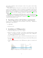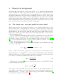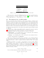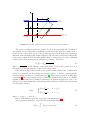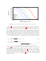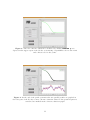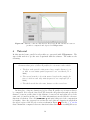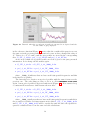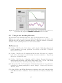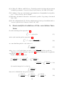
1
PRPgenerator User’s Manual Javier Oliva Quecedo Technical University of Madrid (UPM) Saint Louis University (Madrid Campus) Contents 1 Introduction 1 2 Operating system and hardware requirements 2 3 Installation of PRPgenerator 2 4 Theoretical background 4.1 The classic way: one only profile for every wheel . . . . . . . . . . . . 4.2 The improved way: parallel profiles . . . . . . . . . . . . . . . . . . . 3 3 4 5 Overview 9 6 Tutorial 12 6.1 Using a new working directory . . . . . . . . . . . . . . . . . . . . . . 15 A Semi-analytical solution of the correlation functions 1 16 Introduction PRP stands for Parallel Road Profiles and therefore PRPgenerator generates parallel synthetic road profiles of a given length. The main objective of the generation of parallel profiles along a road stretch is to take into consideration that road profile is not constant along road width and therefore imperfections under left and right tyres of a 4 (or more) wheeled vehicle are different. This fact is frequenlty neglected in road vehicle and bridge dynamics. This simplification can be found both when road profile is measured in situ and also when synthetic profiles are employed. This entails that the road profile is the same under all wheels. Nevertheless, when a four wheeled vehicle runs over a road, left and right wheels do not follow the same path, thus the profiles under each side tyres are different, but those profiles are not independent. Road roughness is a main source of dynamic excitation in road vehicle-bridge dynamics and has an influence on both systems, the vehicle and the bridge. A correct 1 and complete definition of the road surface is then a key point in vehicle–bridge dynamic analysis. Neglecting L-R difference has an effeect on both the vehicle and the bridge. With respect to Vehicle dynamics: vertical acceleration is overestimated, body roll is not gathered, forces under wheels are not accurately determined... In regard to Bridge, dynamic effects are overestimated: accelerations, deflection, Dynamic Amplification Factors.... Influence in vehicle dynamic behaviour is addressed in [1], effects on bridges in [2]. PRPgenerator is implemented in MATLAB and it is a stand-alone application so no MATLAB license or installation is required. The software is introduced in [3] even though its theroretical background is explained in [1, 2], this background is contained in this manual as well. 2 Operating system and hardware requirements Current version of PRPgenerator works in Windows 7/XP/Vista/8. Minimum requirements are expected to be: • 4 GB RAM • 64-bit processor 3 Installation of PRPgenerator 1. Download PRPgenerator.rar to your computer. 2. Extract its content at any folder. A new folder called PRPgenerator should appear. It contains one folder called License and two files: PRPgenerator_Manual.pdf and PRPgenerator_pkg.exe. 3. Double click PRPgenerator_pkg.exe and follow the instructions on the screen. 4. Once the installation has finished new files appear in the folder PRPgenerator (see figure 1) 5. Double click PRPgenerator.exe (not PRPgenerator_pkg.exe) to run the software. Figure 1: PRPgenerator folder with installation completed. 2 4 Theoretical background In site-specific problems the actual road profile can be measured and employed in the calculations. When the actual profile of a particular road stretch is not appropriate but a set of profiles that are representative of a certain sort of roads, stochastic definitions for the generation of synthetic profiles are used. This section in divided in two parts. Firstly, a brief explanation of the generation of simple profiles is presented; this is important because it helps to introduce some concepts and assumptions that will be used in the generation of parallel profiles. In second place, the generation of parallel road profiles is explained. 4.1 The classic way: one only profile for every wheel In this subsection we are interested in how to create rough profiles along a road, these profiles will be independent of each other. Profiles generated in this way are prescribed at every vehicle wheel so the only difference in the imposed vertical displacement at the tyres arises from the time lag between front and rear tyres. This is the common procedure employed in road bridge dynamics so the reader is probably familiar with it. It is a commonly assumed hypothesis that the randomness of the road surface roughness can be represented with a normal stationary ergodic random process described by means of its Power Spectral Density (PSD), also known as G ([4, 5, 6]...). Several PSD functions have been proposed by different authors. A survey of different approximations can be found in [7]. Once a PSD definition has been chosen, road profiles are generated as the sum of a series of harmonics: N X p 2G(ni )∆n cos(2πni x + φi ) r(x) = (1) i where r is the road elevation, G(n) is the one-sided power spectral density for the spatial frequency or wavenumber n and φi is the random phase angle uniformly distributed from 0 to 2π. This expression employs N frequencies between two values nmin and nmax and the increment value (∆n) is set constant: nmax − nmin (2) N ISO-8608 specifications [8] propose a distribution for the one-sided PSD defined by the following expression: −2 n G(n) = G(n0 ) (3) n0 ∆n = where G(n) is the one-sided power spectral density for the spatial frequency or wavenumber n and G(n0 ) is the one-sided power spectral density for the reference spatial frequency n0 = 0.1 m−1 . The value for G(n0 ) is prescribed by ISO-8608 [8] as a function of the road class (Table 1). 3 Road class A (Very good) B (Good) C (Medium) D (Poor) E (Very poor) G(n0 ) [m3 ] 16 · 10−6 64 · 10−6 256 · 10−6 1024 · 10−6 4096 · 10−6 Table 1: Gd (n0 ) for different road classes according to ISO-8608. This expression is adopted in PRPgenerator.Lower and upper spatial frequency limits are set as nmin = 0.01 m−1 and nmax = 10.0 m−1 [8], those limits correspond to wavelength limits λmax = 100 m and λmin = 0.1 m. 4.2 The improved way: parallel profiles When a four wheeled vehicle runs along a road an imposed history of displacement is applied on all its tyres due to the road imperfections. For wheels in the same transverse position, for example the two right wheels, it can be assumed that both run on the same profile. Hence, the imposed displacement is the same but there is a time lag because front tyres reache every point a while before rear ones. On the other hand, tyres that are not transversely aligned, that is to say left and right tyres, run over different paths and therefore the imperfections and the imposed displacements are different. As stated before, different longitudinal profiles computed by means of equation (1) are independent profiles which correspond to one line along the road. PRPgenerator assumes two main hypotheses in regard to road surface: • Homogeneity: every straight profile on the road has the same statistical characteristics, independently of its position. • Isotropy: every straight profile on the road has the same statistical characteristics, independently of its direction. Therefore, in a homogeneous and isotropic road surface every straight profile has the same statistical characteristics, independently of its direction or position. This entails that the surface could be completely described with the PSD of any straight profile. Consider any surface r(x, y) where r is the distance to the Oxy plane and two parallel profiles rL (x) y rR (x) (Left and Right) that are the intersections of the surface with the vertical planes y = b and y = −b respectively (figure 2). This two profiles are defined as functions of x, which is the road longitudinal coordinate. The autocorrelation functions of these profiles RL (δ) and RR (δ) in this kind of process fulfill the following condition: RL (δ) = RD (δ) = R(δ) (4) Cross-correlation functions for these profiles will be also equal: RLR (δ) = RRL (δ) = Rx (δ) 4 (5) Figure 2: Parallel profiles in a homogeneous and isotropic surface. The cross-correlation of the two profiles Rx (δ) is obtained with the elevation of two points, one in each profile, at a distance from each other equal to δ in direction x; that is to say rL (xB ) and rR (xA ). Those points are also related in the autocorrelation function of the straight profile taken along line AB, the autocorrelation of AB profile is the same as that of the Left and Rigth profiles rL and rR since it is also a straight profile on the same homogeneous and isotropic surface. Therefore: p Rx (δ) = R( δ 2 + (2b)2 ) (6) p where δ 2 + (2b)2 is the distance along AB profile between two points at δ in x direction, b is half the distance between the two profiles. PSD function G(n) that describes the profiles must satisfy some conditions in order to be suitable for describing an isotropic surface, it must be monotonically non-increasing and have a bounded integral [9]. Expression proposed in ISO-8608 (equation (3)) does not satisfy isotropy conditions and therefore it has to be slightly modified. If the function is assumed constant at all spatial frequencies below na we will get a piecewise-defined spectral density function that is valid for the description of an isotropic surface: G(n) = n −2 G(n0 )( na0 ) if n ≤ na G(n0 )( nn0 )−2 if n > na (7) where na is set na = 0.01 m−1 . Hence, PSD function gets the appearance shown in figure 3. Autocorrelation function can be derived from PSD function as: Z ∞ R(δ) = G(n) cos(2πδn)dn 0 5 (8) Figure 3: ISO-8608 spectral density function modified in order to represent a homogeneous and isotropic process (logarithmic scale in both axes). And cross-PSD Gx (n) can be obtained from Rx (δ) by means of Fourier transform. Let’s see how to get autocorrelation and cross sorrelation functions from G(n). Given that G(n0 ) and n0 are constant expression 7 can be rewritten as: −2 if n ≤ na cna (9) G(n) = −2 cn if n > na 0) with c = G(n . This simplification makes the explanation easier. n−2 0 Substituting equation 9 into equation 8 the following expression is obtained: Z ∞ −1 sin(2πna δ) −2 n cos(2πnδ)dn (10) R(δ) = 2c na + (2πna δ) na And considering expressions (6) and 10: ! p Z ∞ 2 + (2b)2 ) p sin(2πn δ a p Rx (δ) = 2c n−1 + n−2 cos(2πn δ 2 + (2b)2 )dn (11) a 2 2 (2πna δ + (2b) na Integrals in expressions 10 and 11 are solved semi-analitically as explained in appendix A. This solution is computationally faster than the numerical integration. Once we have computed the cross-correlation function, cross PSD is computated by means of Discrete Fourier Transform: Gx (nk ) = 2 N −1 X 2πi Rx (δn )e− N kn k = 0, 1, ..., N − 1 (12) n=0 Since Rx is unique for a pair of profles, Gx is also unique. Coherence of a pair of profiles can be expressed in this kind of process as: g(n) = |Gx (n)| G(n) given that Gx (n) is real [9]. 6 (13) Coherence 1 0.9 0.8 0.7 0.6 0.5 0.4 2b=0.1 m 0.3 2b=0.5 m 0.2 2b=1 m 0.1 2b=2 m 2b=4 m 0 0.01 0.1 1 10 −1 Spatial frequency [m ] Figure 4: Coherence function for different distances between profiles. Figure 4 shows coherence functions for different distances between profiles. Actually, coherence function defined in expression (13) is independent of c, therefore it will not depend on the road class but only on the distance between profiles. Coherence is higher for small spatial frequencies or high wavelengths and gets significantly lower for high spatial frequencies or reduced wavelengths. This is quite feasible since high wavelength imperfections affect to a higher width than small wavelength imperfections that are more localized. We can also appreciate that coherence is lower for all wavelengths if the distance between profiles is increased which is also logical. Once cross-PSD Gx (n) has been computed the two parallel profiles are obtained as: N X p 2G(ni )∆n cos(2πni x + φi ) rL (x) = (14a) i N h X p rR (x) = 2G(ni )∆n cos(2πni x + φi ) + (14b) i i p + 2(G(ni ) − Gx (ni ))∆n cos(2πni x + θi ) where φi and θi are random phase angles uniformly distributed from 0 to 2π. Figure 5 shows parallel Class A profiles at different distances generated with PRPgenerator. The PSD of those profiles is computed, smoothed according to ISO8608 and compared with the ISO definition (Eq. (3)). The lower is the distance between profiles the higher is the similarity, as it is expected. As can be seen PSD agreement is excellent. If the road stretch length is higher the computation of PSD will be more accurate as can be seen in figure 6 where the road section considered is 400 meters long. 7 Power Spectral Density [m3] Elevation [mm] 1e−02 20 15 10 5 0 −5 −10 −15 −20 Left profile Right profile 0 20 40 60 80 Class A (ISO−8608) Left profile Right profile 1e−03 1e−04 1e−05 1e−06 1e−07 1e−08 1e−09 0.01 100 0.1 1 10 Spatial frequency [m−1] Distance [m] 1e−02 20 15 10 5 0 −5 −10 −15 −20 Power Spectral Density [m3] Elevation [mm] (a) Distance = 0.1 m Left profile Right profile 0 20 40 60 80 Class A (ISO−8608) Left profile Right profile 1e−03 1e−04 1e−05 1e−06 1e−07 1e−08 1e−09 0.01 100 0.1 1 10 Spatial frequency [m−1] Distance [m] (b) Distance = 2.0 m Left profile Right profile 10 Elevation [mm] Power Spectral Density [m3] 1e−02 15 5 0 −5 −10 −15 0 20 40 60 80 100 Class A (ISO−8608) Left profile Right profile 1e−03 1e−04 1e−05 1e−06 1e−07 1e−08 1e−09 0.01 0.1 1 10 Spatial frequency [m−1] Distance [m] (c) Distance = 4.0 m Figure 5: Parallel Class A Road Profiles and their Power Spectral Densities. Power Spectral Density [m3] 1e−02 Class A (ISO−8608) Left PSD Right PSD 1e−03 1e−04 1e−05 1e−06 1e−07 1e−08 1e−09 0.01 0.1 1 10 Spatial frequency [m−1] Figure 6: Power Spectral Density of two 400 meters long parallel road profiles (class A). 8 5 Overview PRPgenerator is quite simple and intuitive. Its main and only window in shown in figure 7. We can distinguish the following parts: • PRPgenerator logo on the left-hand upper corner. • Problem data section on the left side. Here is where the user defines the properties of the profiles that are to be generated. • Results section on the right-hand side. In this section some results are depicted: coherence function in the upper window and the generated profiles in the lower one. • Two buttons, COMPUTE g and GENERATE PROFILES, are located on the left-hand lower corner. Figure 7: Initial appearance of the main and only window of PRPgenerator The following parameters are set by the user in the Problem data section: Road class according to ISO-8608. One option in the drop-down list has to be chosen; available road classes range from Very good (A) to Very poor (E). 9 Distance between profiles in meters. In general it will correspond with the vehicle width or, more precisely, with the axle track (distance between the centerline of two wheels on the same axle). Road stretch length in meters. This is the length of the profiles to be generated. Sample distance in meters. Since 0.1 m is the lower considered wavelength, the distance between samples in the generated profiles should not be higher than 0.02 m. Number of frequencies (or equivalently wavelengths) to be used in the profile generation. This value corresponds to the N in expression (14). This value must be large enough if we want to get a good profile description, N = 2000 is a good choice. There are two buttons on the lower left corner of the PRPgenerator window: COMPUTE g and GENERATE PROFILES: • COMPUTE g calculates Gx (n) and the coherence function g(n). At the end of the computation, coherence function is depicted in the correponding region of the Results section (see figure 8). Coherence function is stored in the working directory as an ascii file named g_[Distance between profiles]_[Road class label].dat. The Road class label is the value of G(n0 ) in table 1 multiplied by 106 , that is to say Class A=16, Class B=64, Class C=256, Class D=1024, Class E=4096. For example g_2.2_16.dat is the coherence function for a distance between profiles equal to 2.2 meters and Road class A. This file is organized into two columns: (1) spatial frequency n [m−1 ] and (2) coherence function g. For the computation of g(n) only Road class and Distance between profiles are needed so the other fields can remain unspecified at this point. • GENERATE PROFILES does what it says. Road section length, sample distance and number of frequencies are needed now. When this button is clicked profiles are generated and depicted in the lower part of the Results section (figure 9). The values of g employed in the generation, that will depend on the Number of frequencies considered, are marked as black circles over the coherence function obtained before. Those values are saved in G_GX_[Distance between profiles]_[Road class label].dat along with the values of G and GX . This file is organized into 4 columns: (1) Frequency n [m−1 ], (2) G [m3 ], (3) GX [m3 ] and (4) g. Profiles are saved in two files named prof_[Distance between profiles]_[Road class label]_[Side label].dat where Side label is LF for the left profile and RT for the right one. Profile files are organized in two columns: (1) Distance to the origin [m] and (2) Profile elevation [m]. If GENERATE PROFILES is clicked again a new pair of profiles is generated, depicted and saved. They will be stored in files with the same names as the previous profiles so these will be overwritten and therefore lost. If we want to create several profiles, as is usual, the procedure is: (1) Generate, (2) Protect the files by changing their names or moving them to another folder, (3) Generate another pair of profiles, (4) Repeat this actions as many times as necessary. 10 Figure 8: Once the coherence function is calculated by clicking COMPUTE g it is depicted in the upper region of the Results section using a logarithmic scale for the x-axis and a linear scale for the y-axis. Figure 9: At the end of the profile generation the two parallel profiles are graphed in the lower part of the Results section, coherence function values for the spatial frequencies considered are marked in the coherence function graph. 11 Figure 10: Tutorial: coherence function for Road class B and 2.0 meters between profiles is computed and depicted in PRPgenerator. 6 Tutorial In this tutorial some parallel road profiles are generated with PRPgenerator. The aim of this work is to get the user acquainted with the software. The tasks are the following: Generate three pairs of Class B profiles for a 2 meters wide vehicle: 1. The first road stretch is 100 meters long, sample distance is set as 0.01 m and 2000 spatial frequencies are considered (N = 2000). 2. The second stretch is also 100 meters long but the sample distance is 0.02 m and only 1000 frequencies are employed (N = 1000). 3. The third stretch has the same features as the second one. In first place coherence function g(n) for Class B profiles at 2.0 meters has to be computed. Select Road class Good (B) from the drop-down list and specify the distance between profiles that is the distance between left and right tyres of the same axle, 2.0 meters in this case. No other information is needed for the coherence function calculation. Now click COMPUTE g and wait (this part of the computation is lengthy). Once the progress bar reaches the end coherence function is graphed in the upper region of the Results section as shown in Figure 10. The file g_2_64.dat that contains the computed coherence function is then saved in the working directory. 12 Figure 11: Tutorial: after clicking GENERATE PROFILES they are depicted in the bottom right-hand window, values of the coherence function employed in the generation are marked in the coherence function window. Notice that your upper graph must be the same as the one in this figure but not the lower one due to the randomness of the synthetic profiles. Now you can generate your pairs of profiles. Let’s start with the first profile. Set Road stretch length equal to 100 meters, Sample distance equal to 0.01 meters and a Number of frequencies of 2000. Click GENERATE PROFILES. Profile generation is much faster than coherence function computation so you do not have to be as patient as in the previous step. When the calculation is finished profiles are depicted in the lower part of the Results section and the employed values of g(n) are marked over the coherence function graph (Figure 11). The software creates G_GX_2_64.dat in which the 2000 considered frequencies and the corresponding values of G, Gx and g are stored. Left profile is saved in prof_2_64_LF.dat and right profile in prof_2_64_RT.dat. Since we have been told to generate another pair of profiles we need to protect the just created files, otherwise they would be overwritten and the generated profiles lost. We may change their names or move them to another directory. Let’s change their names as follows1 : • G_GX_2_64.dat → G_GX_2_64_2000.dat • prof_2_64_LF.dat → prof_2_64_LF_2000.dat • prof_2_64_RT.dat → prof_2_64_RT_2000.dat where _2000 indicates that we have used 2000 spatial frequencies. In order to generate the second road section we need to change the values of sample distance (0.02 m) and number of frequencies (1000). Then click GENERATE PROFILES. The new profiles are depicted and the considered frequencies are shown 1 This is just an example, any notation can be adopted. 13 Figure 12: Tutorial: when the second pair of profiles is generated it is depicted and also are the values of g(n) employed. in the coherence function (Figure 12); notice that the considered frequencies are not the same as in the previous profile generation because we have changed the value of N . Values of n, G, Gx and g and the new profiles are stored in the corresponding files: G_GX_2_64.dat, prof_2_64_LF.dat and prof_2_64_RT.dat. As we need a third set of parallel profiles we need to protect the just generated information. Let’s change the file names again: • G_GX_2_64.dat → G_GX_2_64_1000_1.dat • prof_2_64_LF.dat → prof_2_64_LF_1000_1.dat • prof_2_64_RT.dat → prof_2_64_RT_1000_1.dat where _1000_1 indicates that we have used 1000 spatial frequencies and this is the first set of profiles. The last task is to obtain a new pair of profiles with the same features as the previous one. The only thing we have to do is to click GENERATE PROFILES again. A new pair of profiles is depicted and stored (Figure 13). If we want to keep a consistent file notation we shall rename the new files: • G_GX_2_64.dat → G_GX_2_64_1000_2.dat • prof_2_64_LF.dat → prof_2_64_LF_1000_2.dat • prof_2_64_RT.dat → prof_2_64_RT_1000_2.dat where _1000_2 indicates that we have used 1000 spatial frequencies and this is the second set of profiles. It is important to notice that G_GX_2_64_1000_2.dat and G_GX_2_64_1000_2.dat will be exactly the same file since the Spatial frequencies considered have been the same in both calculations. 14 Figure 13: Tutorial: a ner pair of profiles with the same properties as the previous one is generated and graphed if GENERATE PROFILES is clicked again. 6.1 Using a new working directory If you want to work in another directory just copy PRPgenerator.exe (not PRPgenerator_pkg.exe) and the License folder into that directory and double click PRPgenerator.exe on that new working directory. Thus the software is run there and files created by PRPgenerator are saved to that folder. References [1] J. Oliva, J. M. Goicolea, M. A. Astiz, and P. Antolín. Fully three-dimensional vehicle dynamics over rough pavement. Proceedings of the ICE - Transport, 166(3):144–157, 2013. [2] J. Oliva, J. M. Goicolea, P. Antolín, and M. A. Astiz. Relevance of a complete road surface description in vehicle-bridge interaction dynamics. Engineering Structutres, 56:466–476, 2013. [3] J. Oliva, J. M. Goicolea, P. Antolín, and M. A. Astiz. Dynamic behaviour of underspanned suspension road bridges under traffic loads. Journal of the South African Institution of Civil Engineering, 56(3):77–87, 2014. [4] L. Deng and C. S. Cai. Development of dynamic impact factor for performance evaluation of existing multi-girder concrete bridges. Engineering Structures, 32:21–31, 2010. [5] L. Ding, H. Hao, and X. Zhu. Evaluation of dynamic vehicle axle loads on bridges with different surface conditions. Journal of Sound and Vibration, 323:826–848, 2009. 15 [6] A. Belay, E. O’Brien, and D. Kroese. Truck fleet model for design and assessment of flexible pavements. Journal of Sound and Vibration, 311:1161–1174, 2008. [7] P. Andrén. Power spectral density approximations of longitudinal road profiles. Int. J. Vehicle Design, 40:2–14, 2006. [8] ISO-8608. Mechanical vibration - Road surface profiles - Reporting of measured data. 1995. [9] K. M. A. Kamash and J. D. Robson. Implications of isotropy in random surfaces. Journal of Sound and Vibration, 54:131–145, 1977. A Semi-analytical solution of the correlation functions Second term integral in expression (10): Z ∞ n−2 cos(2πnδ)dn (15) na and second term integral in expression (11): Z ∞ p n−2 cos(2πn δ 2 + (2b)2 )dn (16) na are same kind integrals for each value of δ: Z ∞ cos(an) dn (17) n2 na p where a is a = 2πδ in the first case and a = 2π δ 2 + (2b)2 in the second one. Therefore we need to integrate expression 17 and the solution will be applied to expressions (15) and (16). Firstly we integrate by parts: Z ∞ na ∞ Z ∞ cos(an) cos(an) sin(an) dn = − − a dn n2 n n na na Z ∞ cos(ana ) sin(an) = −a dn (18) na n na So now the integral to be solved is: Z ∞ na sin(an) dn n that can be divided into two parts as follows: Z ∞ Z ∞ Z na sin(an) sin(an) sin(an) dn = dn − dn n n n na 0 0 16 (19) (20) Si(x) 2 1.8 1.6 1.4 1.2 1 0.8 0.6 0.4 0.2 0 π/2 0 2 4 6 8 10 12 14 16 x Figure 14: Dirichlet Integral. Let’s stop here to study the integral of function sin(n) . Indefinite integral of this n function does not exist in closed-form. Nevertheless, the definite integral with upper and lower limits equal to 0 and x respectively defines a new function of x known as Sine Integral : Z x sin(n) dn (21) Si(x) = n 0 We can approximate this function by using McLaurin series expansion of sin(n): sin(n) ' n − n3 n5 + − ... 3! 5! (22) The integrand turns into: n2 n4 sin(n) '1− + − ... (23) n 3! 5! And the integral becomes: Z x Z x sin(n) n2 n4 x3 x5 Si(x) = dn ' 1− + − ... dn = x − + − ... (24) n 3! 5! 3 · 3! 5 · 5! 0 0 a series that converges for all x. If we plot this approximation (figure 14) we can see that the sine integral tends to π2 when x tends to ∞. Hence: Z ∞ sin(n) π lim Si(x) = dn = (25) x→∞ n 2 0 This expression is known as Dirichlet integral, after the German mathematician Johann Peter Gustav Lejeune Dirichlet2 If we substitute sin(n) with sin(an) where a is constant it is easy to demonstrate the following: π if a > 0 2 Z ∞ sin(an) 0 if a = 0 dn = (26) n 0 π −2 if a < 0 2 Actually, there are several integrals with this name; this is one of them. 17 It is trivial to prove that a will always be positive or null. Let’s go back to the expression 20: Z ∞ Z na Z ∞ sin(an) sin(an) sin(an) dn = dn − dn n n n 0 0 na The first term in the right-hand is solved by means of equation 26. The second term can be approximated by using McLaurin series expansion: Z na sin(an) (ana )3 (ana )5 dn = ana − + − ... = Si(ana ) (27) n 3 · 3! 5 · 5! 0 Substituting equations 26 and 27 in expression 20: π Z ∞ 2 − Si(ana ) si a > 0 sin(an) dn = n na 0 − Si(ana ) si a = 0 where Si(ana ) is computed by means of McLaurin series expansion. With expression (28) we can solve the initial integral (equation (18)): Z ∞ hπ i cos(an) cos(ana ) dn = − a − Si(an ) a n2 na 2 na (28) (29) It is important to notice that the piecewise expression in equation (28) vanished in equation (29), the reason is that the second term in the right-hand side will be always zero if a = 0 so it is not necessary to make a distinction and the expression can be simplified. Therefore, integral in expression (15) where a = 2πδ is solved as follows: Z ∞ hπ i cos(2πnδ) cos(2πna δ) dn = − 2πδ − Si(2πna δ) (30) n2 na 2 na p And integral in expression (16) in which a = 2π δ 2 + (2b)2 : Z ∞ na p cos(2πn δ 2 + (2b)2 ) dn = n2 p hπ i p p cos(2πna δ 2 + (2b)2 ) = − 2π δ 2 + (2b)2 − Si(2πna δ 2 + (2b)2 (31) na 2 18