Download User Guide: Imaging

User Guide:
Imaging
Horizontal and Micro NMR Imaging
With VNMR 6.1C Software
Pub. No. 01-999163-00, Rev. A0800
User Guide: Imaging
Horizontal and Micro NMR Imaging
With VNMR 6.1C Software
Pub. No. 01-999163-00, Rev. A0800
Revision history:
A0800 – Initial release for VNMR 6.1C.
Applicability of manual:
Imaging modules on Varian NMR superconducting spectrometer systems with
VnmrIMAGE version 4.4 software installed.
Technical contributors: Simon Chu, Matt Howitt, Chris Price, Alan Rath,
Subramaniam Sukumar, Evan Williams
Technical writers: Michael Carlisle, Dan Steele
Technical editor: Dan Steele
Copyright 2000 by Varian, Inc.
3120 Hansen Way, Palo Alto, California 94304
http://www.varianinc.com
All rights reserved. Printed in the United States.
The information in this document has been carefully checked and is believed to be
entirely reliable. However, no responsibility is assumed for inaccuracies. Statements in
this document are not intended to create any warranty, expressed or implied.
Specifications and performance characteristics of the software described in this manual
may be changed at any time without notice. Varian reserves the right to make changes in
any products herein to improve reliability, function, or design. Varian does not assume
any liability arising out of the application or use of any product or circuit described
herein; neither does it convey any license under its patent rights nor the rights of others.
Inclusion in this document does not imply that any particular feature is standard on the
instrument.
UNITY
INOVA, MERCURY-VX, MERCURY, Gemini, GEMINI 2000, UNITYplus, UNITY,
VXR, XL, VNMR, VnmrS, VnmrX, VnmrI, VnmrV, VnmrSGI, MAGICAL II,
AutoLock, AutoShim, AutoPhase, limNET, ASM, and SMS are registered trademarks or
trademarks of Varian, Inc. Sun, Solaris, CDE, Suninstall, Ultra, SPARC, SPARCstation,
SunCD, and NFS are registered trademarks or trademarks of Sun Microsystems, Inc. and
SPARC International. Oxford is a registered trademark of Oxford Instruments LTD.
Ethernet is a registered trademark of Xerox Corporation. VxWORKS and VxWORKS
POWERED are registered trademarks of WindRiver Inc. Other product names in this
document are registered trademarks or trademarks of their respective holders.
Overview of Contents
SAFETY PRECAUTIONS ................................................................................. 11
Introduction ..................................................................................................... 15
Chapter 1. First Steps: Making an Image ..................................................... 17
Chapter 2. Imaging Experiments .................................................................. 25
Chapter 3. Imaging Pulse Sequences .......................................................... 41
Chapter 4. Image Browser ............................................................................. 65
Chapter 5. Image Browser Math Processing ............................................. 111
Chapter 6. CSI Data Processing .................................................................. 129
Chapter 7. High-Performance Auxiliary and Microimaging Gradients .... 175
Chapter 8. Digital Eddy Current Compensation ........................................ 199
Chapter 9. Physiological Gating Module .................................................... 207
Chapter 10. 2D and 3D Backprojection ...................................................... 225
Chapter 11. Interactive Image Planning ..................................................... 253
Appendix A. Commands, Macros, and Parameters .................................... 255
Index ............................................................................................................... 347
01-999163-00 A0800
VNMR 6.1C User Guide: Imaging
3
4
VNMR 6.1C User Guide: Imaging
01-999163-00 A0800
Table of Contents
SAFETY PRECAUTIONS ................................................................................. 11
Introduction ..................................................................................................... 15
Chapter 1. First Steps: Making an Image ..................................................... 17
1.1 Making an Initial Scout Image .................................................................................... 17
1.2 Using the Scout Image to Plan a New Target Image ................................................... 22
Chapter 2. Imaging Experiments .................................................................. 25
2.1
2.2
2.3
2.4
2.5
2.6
2.7
2.8
2.9
Basic Imaging Principles ............................................................................................
Time Domain to Spatial Domain Conversion .............................................................
Slice Selection .............................................................................................................
Frequency Encoding ...................................................................................................
Phase Encoding ...........................................................................................................
Image Resolution ........................................................................................................
Spatial Frame of Reference .........................................................................................
Image Reconstruction .................................................................................................
Important Imaging Parameters ....................................................................................
25
26
29
32
34
35
37
38
38
Chapter 3. Imaging Pulse Sequences .......................................................... 41
3.1
3.2
3.3
3.4
3.5
3.6
Initial Setup .................................................................................................................
Conditions for Use ......................................................................................................
GEMS Multislice Imaging ..........................................................................................
Obtaining a GEMS Image ...........................................................................................
Echo Planar Imaging and Phase Correction Map Files ..............................................
Commands, Macros, and Parameters ..........................................................................
41
42
44
49
51
62
Chapter 4. Image Browser ............................................................................. 65
4.1
4.2
4.3
4.4
4.5
4.6
Overview ..................................................................................................................... 65
Getting Started ............................................................................................................ 68
Graphics Tools ............................................................................................................ 80
Data Processing ........................................................................................................... 90
Macros ......................................................................................................................... 98
Files and Other Items ................................................................................................ 104
Chapter 5. Image Browser Math Processing ............................................. 111
5.1
5.2
5.3
5.4
5.5
Opening Image Browser Math ..................................................................................
Image Browser Math Expressions ............................................................................
Image Browser Math Functions ................................................................................
The Fit Program ........................................................................................................
Problems with Image Browser Math ........................................................................
111
112
113
120
127
Chapter 6. CSI Data Processing .................................................................. 129
6.1 Overview of CSI ....................................................................................................... 129
01-999163-00 A0800
VNMR 6.1C User Guide: Imaging
5
Table of Contents
6.2
6.3
6.4
6.5
Getting Started ..........................................................................................................
Tools ..........................................................................................................................
Processing Functions ................................................................................................
Files and Other Items ................................................................................................
133
147
156
167
Chapter 7. High-Performance Auxiliary and Microimaging Gradients .... 175
7.1
7.2
7.3
7.4
HPAG-183 Hardware ................................................................................................
Experimental Setup ...................................................................................................
Performance Specifications .......................................................................................
Microimaging Hardware ...........................................................................................
175
183
189
190
Chapter 8. Digital Eddy Current Compensation ........................................ 199
8.1
8.2
8.3
8.4
The DECC Module ...................................................................................................
Theory of Preemphasis .............................................................................................
Using the decctool Interface .....................................................................................
Exercising decctool Using an Oscilloscope ..............................................................
199
199
202
206
Chapter 9. Physiological Gating Module .................................................... 207
9.1
9.2
9.3
9.4
Cardiac Anatomy and Electrocardiography ..............................................................
Hardware Description ...............................................................................................
Experimental Setup ...................................................................................................
Performance Specifications .......................................................................................
207
209
216
223
Chapter 10. 2D and 3D Backprojection ...................................................... 225
10.1
10.2
10.3
10.4
10.5
10.6
10.7
Installation ...............................................................................................................
Backprojection Image Generation ..........................................................................
Getting Started ........................................................................................................
Routine Usage .........................................................................................................
Artifacts in BP Imaging ..........................................................................................
BP Macros and Programs Details ...........................................................................
References ...............................................................................................................
225
226
227
229
244
249
252
Chapter 11. Interactive Image Planning ..................................................... 253
11.1 Introduction ............................................................................................................. 253
11.2 Starting the Planning Session .................................................................................. 253
Index ............................................................................................................... 347
6
VNMR 6.1C User Guide: Imaging
01-999163-00 A0800
List of Figures
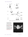
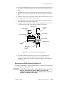
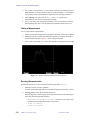
Figure 1. Frequency Spectrum Produced by an NMR Signal ......................................................
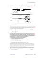
Figure 2. Effect of a Field Gradient Along Direction y ................................................................
Figure 3. Frequency Ranges .........................................................................................................
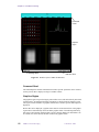
Figure 4. 2D Image Resulting from a Slice Selection ..................................................................
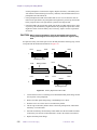
Figure 5. Rectangular Profile ........................................................................................................
Figure 6. Slice Profile ...................................................................................................................
Figure 7. Sinc Function, Truncated Sinc Pulse, and Gaussian-Shaped Slice Profiles ..................
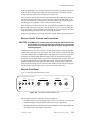
Figure 8. Multislice Excitation .....................................................................................................
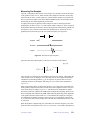
Figure 9. Signal Loss Restoration .................................................................................................
Figure 10. Readout Gradient and Gradient Echo ..........................................................................
Figure 11. Gradient Echo Imaging Sequence ...............................................................................
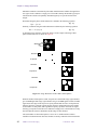
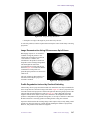
Figure 12. Image Resolution of Three Water-Filled Spheres .......................................................
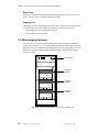
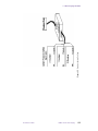
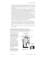
Figure 13. Horizontal Magnet .......................................................................................................
Figure 14. Vertical Magnet ...........................................................................................................
Figure 15. Signal Intensity ............................................................................................................
Figure 16. Equilibrium Magnetization .........................................................................................
Figure 17. Gradient Echo Imaging Sequence ...............................................................................
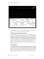
Figure 18. Gradient-Echo Version of EPI Pulse Sequence ...........................................................
Figure 19. Spin-Echo Variant of the EPI Pulse Sequence ............................................................
Figure 21. Ghost Artifact ..............................................................................................................
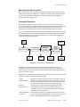
Figure 20. Time Domain Data Processing Steps ..........................................................................
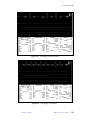
Figure 22. EPI Echo Train ............................................................................................................
Figure 23. Echo Train After groa Adjustment ..............................................................................
Figure 24. Aligned Echoes ............................................................................................................
Figure 25. Centered Echoes ..........................................................................................................
Figure 25. Default Layout of Main Image Browser Screen .........................................................
Figure 26. Image Browser Control Panel .....................................................................................
Figure 27. Frame Properties Menu ...............................................................................................
Figure 28. Zoom Magnification Factor Window ..........................................................................
Figure 29. Tools Window ..............................................................................................................
Figure 30. Vertical Scale Properties Window ...............................................................................
Figure 31. Vertical Scaling Window .............................................................................................
Figure 32. Curve Control Point ....................................................................................................
Figure 33. Gamma Correction Window ........................................................................................
Figure 34. Statistics Window with One ROI .................................................................................
Figure 35. Statistics Window with Multiple ROIs ........................................................................
Figure 36. 3D Volume Calculations ..............................................................................................
Figure 37. Statistics Output Generated by Print Stats Button ......................................................
Figure 38. Rotation Panel .............................................................................................................
Figure 39. Filter Window ..............................................................................................................
Figure 40. Filter Window with Data .............................................................................................
Figure 41. Histogram Window ......................................................................................................
01-999163-00 A0800
VNMR 6.1C User Guide: Imaging
26
27
28
29
29
30
30
31
32
33
34
36
37
38
39
40
45
53
54
54
55
60
60
60
60
66
70
71
79
80
82
83
84
85
91
93
93
94
95
96
96
97
7
List of Figures
Figure 42. Cursor Data Window ................................................................................................... 97
Figure 43. Line Data Window ....................................................................................................... 97
Figure 44. Macro Window ............................................................................................................ 98
Figure 45. File Browser for Loading Images .............................................................................. 104
Figure 46. Slice Extraction Window ........................................................................................... 105
Figure 47. Image Browser Math Panel ....................................................................................... 111
Figure 48. Fragment of shamesfit.c File ............................................................................. 125
Figure 49. FUNCTION Specifications ....................................................................................... 125
Figure 50. JACOBIAN Definition .............................................................................................. 126
Figure 51. GUESS Signature ...................................................................................................... 126
Figure 52. Default Layout of Main CSI Windows ...................................................................... 130
Figure 53. Processing Functions Data Flow ............................................................................... 131
Figure 54. CSI Command Panel ................................................................................................. 135
Figure 55. Graphics Tools Window ............................................................................................ 136
Figure 56. Frame Props Window ................................................................................................ 136
Figure 57. CSI Data Basic Processing Steps .............................................................................. 139
Figure 58. Filtering Display ........................................................................................................ 140
Figure 59. Phase Correction Window ......................................................................................... 141
Figure 60. Baseline Correction Window ..................................................................................... 142
Figure 61. Metabolic Map Calculation ....................................................................................... 144
Figure 62. Selected Voxels and Curve-Fitted Data ..................................................................... 145
Figure 63. Detailed Data Flow for Metabolic Map Processing .................................................. 145
Figure 64. Image Calctool Window ............................................................................................ 146
Figure 65. Save Check Window .................................................................................................. 146
Figure 66. Graphics Tools Window ............................................................................................ 147
Figure 67. Vertical Scale Properties Window ............................................................................. 148
Figure 68. Vertical Scaling Window ........................................................................................... 149
Figure 69. Curve Control Point .................................................................................................. 150
Figure 70. Gamma Correction Window ...................................................................................... 151
Figure 71. Spatial Reconstruction Window ................................................................................ 157
Figure 72. Spectral Reconstruction Window .............................................................................. 158
Figure 73. Interactive Fitting Tool Window ................................................................................ 163
Figure 74. Metabolic Map Display Window .............................................................................. 164
Figure 75. Image Reconstruction Window ................................................................................. 165
Figure 76. pH Map Control Window .......................................................................................... 166
Figure 77. FileBrowser Window ................................................................................................. 168
Figure 78. FileBrowser Save Tool Window ................................................................................ 169
Figure 79. Colormap Display Window ....................................................................................... 170
Figure 80. Display Control Window ........................................................................................... 170
Figure 81. Sample Prior Knowledge PEAK File ........................................................................ 174
Figure 82. RF Shield Fitted on 183-mm HPAG Gradient Coil ................................................... 177
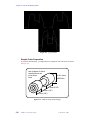
Figure 83. Rear Housing of 183-mm HPAG Gradient Coil ........................................................ 177
Figure 84. HPAG Quick-Disconnect Box ................................................................................... 179
Figure 85. System Gradient Coil Detail of Connection Points ................................................... 180
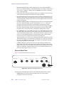
Figure 86. Front Panel of System Gradient Supply .................................................................... 182
Figure 87. Gradient Supply Internal Card Cage ......................................................................... 182
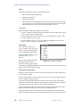
Figure 88. Connections for System Gradient Coil in Standard Configuration ........................... 184
Figure 89. Connections for Auxiliary Configuration .................................................................. 185
8
VNMR 6.1C User Guide: Imaging
01-999163-00 A0800
List of Figures
Figure 90. Microimaging Cabinet with Gradient Control System .............................................
Figure 91. Gradient Compensation Signal Flow ........................................................................
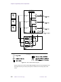
Figure 92. Gradient System Cabling ..........................................................................................
Figure 93. eccTool Window ........................................................................................................
Figure 94. eccTool Files Window ...............................................................................................
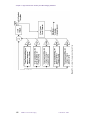
Figure 95. DECC Module Block Diagram .................................................................................
Figure 96. RF Pulse-Acquire Sequence ......................................................................................
Figure 97. decctool Window .......................................................................................................
Figure 98. eccGraph Window .....................................................................................................
Figure 99. Cardiac Anatomy .......................................................................................................
Figure 100. ECG Interpretation ..................................................................................................
Figure 101. Front Panel of Cardiac Preamplifier ........................................................................
Figure 102. Rear Panel of Cardiac Preamplifier .........................................................................
Figure 103. Battery Replacement Procedure ..............................................................................
Figure 104. Front Panel of PGM-1000 Receiver ........................................................................
Figure 105. Back Panel of PGM-1000 Receiver ........................................................................
Figure 106. Electrodes Connection .............................................................................................
Figure 107. Unit Interconnection Diagram .................................................................................
Figure 108. ECG and Inhibit Out: Trigger on (A) Each Heart Beat, (B) Every Other Beat .......
Figure 109. Image Generation Using Backprojection ................................................................
Figure 110. Parameter Set for bp2d ............................................................................................
Figure 111. Profile of Fourier Transform of One Projection ......................................................
Figure 112. Setting the Weighting ..............................................................................................
Figure 113. Unweighted and Weighted Fourier Transform ........................................................
Figure 114. Parameters for Sequence dp_image ........................................................................
Figure 115. On-Resonance Condition ........................................................................................
Figure 116. Macro bp_setup Values Display ..............................................................................
Figure 117. Phases: (A) Preparation and (B) Acquisition ..........................................................
Figure 118. T2 Weighted 2D and 3D Pulse Sequence ................................................................
Figure 119. T1 Weighting–Preparation Phase ............................................................................
Figure 120. T1 Weighting–aps Sequence ...................................................................................
Figure 121. T1rho Weighting ......................................................................................................
Figure 122. Slice-based BP Acquisition .....................................................................................
Figure 123. T2 Weighted 2D Slice-Selective Pulse Sequence ....................................................
Figure 124. T1 Weighting–Inversion or Saturation Recovery ....................................................
Figure 125. T1 Weighting–Inversion or Saturation Recovery ....................................................
Figure 126. Distorted Images .....................................................................................................
Figure 127. Saturation in First Projection ...................................................................................
Figure 128. Circular or Spherical Modulation ............................................................................
Figure 129. Image Intensity Modulation ....................................................................................
Figure 130. Misaligned Profiles ..................................................................................................
Figure 131. B0 Field Shift ...........................................................................................................
Figure 132. Phantom Setup for BP Imaging ...............................................................................
Figure 133. Interactive Image Planning Interface .......................................................................
01-999163-00 A0800
VNMR 6.1C User Guide: Imaging
190
192
193
195
196
200
201
202
206
208
209
211
211
212
213
214
215
217
221
226
227
228
231
232
234
235
236
237
238
239
239
240
241
241
242
243
245
246
246
247
247
248
248
253
9
List of Tables
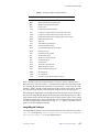
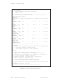
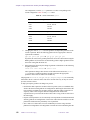
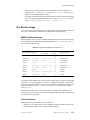
Table 1. Experimental Macros and Parameters ............................................................................. 32
Table 2. Relaxation Times ............................................................................................................. 39
Table 3. EPI Related Commands and Parameters .......................................................................... 52
Table 4. Imaging Parameters ......................................................................................................... 59
Table 5. Imaging Pulse Sequence Commands, Macros, and Parameters ...................................... 62
Table 6. ROI Selector Tool Properties ........................................................................................... 88
Table 7. Formats Available in Image Browser ............................................................................. 107
Table 8. Fit Types ......................................................................................................................... 121
Table 9. Prior Knowledge Menu Selections with Corresponding File Names ............................ 173
Table 10. HPAG-183 Accessory Parts List .................................................................................. 176
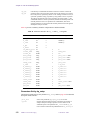
Table 11. Values of Parameter gcoil ......................................................................................... 188
Table 12. Gradient Coil Length and Weight. ............................................................................... 189
Table 13. Gradient Channels Duty Cycles ................................................................................... 189
Table 14. Eddy Current Interface Commands and Parameters .................................................... 191
Table 15. Slew Rate Control ........................................................................................................ 194
Table 16. decctool Macros, and Parameters ............................................................................... 202
Table 17. PGM-1000 Parts List ................................................................................................... 210
Table 18. Cardiac Preamplifier Electrode Connections ............................................................... 211
Table 19. PGM-1000 Performance Specifications ....................................................................... 223
Table 20. Implemented NMR Excitation Schemes ...................................................................... 229
Table 21. Estimated Acquisition and Reconstruction Times ...................................................... 230
Table 22. Parameters Passed to the bp_2d and bp_3d Programs ............................................. 250
Table 23. iplan Controls ........................................................................................................... 254
01-999163-00 A0800
VNMR 6.1C User Guide: Imaging
10
SAFETY PRECAUTIONS
SAFETY PRECAUTIONS
The following warning and caution notices illustrate the style used in Varian manuals for
safety precaution notices and explain when each type is used:
WARNING: Warnings are used when failure to observe instructions or precautions
could result in injury or death to humans or animals, or significant
property damage.
CAUTION:
Cautions are used when failure to observe instructions could result in
serious damage to equipment or loss of data.
Warning Notices
Observe the following precautions during installation, operation, maintenance, and repair
of the instrument. Failure to comply with these warnings, or with specific warnings
elsewhere in Varian manuals, violates safety standards of design, manufacturing, and
intended use of the instrument. Varian assumes no liability for customer failure to comply
with these precautions.
WARNING: Persons with implanted or attached medical devices such as
pacemakers and prosthetic parts must remain outside the 5-gauss
perimeter from the centerline of the magnet.
The superconducting magnet system generates strong magnetic fields that can
affect operation of some cardiac pacemakers or harm implanted or attached
devices such as prosthetic parts and metal blood vessel clips and clamps.
Pacemaker wearers should consult the user manual provided by the pacemaker
manufacturer or contact the pacemaker manufacturer to determine the effect on
a specific pacemaker. Pacemaker wearers should also always notify their
physician and discuss the health risks of being in proximity to magnetic fields.
Wearers of metal prosthetics and implants should contact their physician to
determine if a danger exists.
Refer to the manuals supplied with the magnet for the size of a typical 5-gauss
stray field. This gauss level should be checked after the magnet is installed.
WARNING: Keep metal objects outside the 10-gauss perimeter from the centerline
of the magnet.
The strong magnetic field surrounding the magnet attracts objects containing
steel, iron, or other ferromagnetic materials, which includes most ordinary
tools, electronic equipment, compressed gas cylinders, steel chairs, and steel
carts. Unless restrained, such objects can suddenly fly towards the magnet,
causing possible personal injury and extensive damage to the probe, dewar, and
superconducting solenoid. The greater the mass of the object, the more the
magnet attracts the object.
Only nonferromagnetic materials—plastics, aluminum, wood, nonmagnetic
stainless steel, etc.—should be used in the area around the magnet. If an object
is stuck to the magnet surface and cannot easily be removed by hand, contact
Varian service for assistance.
01-999163-00 A0800
VNMR 6.1C User Guide: Imaging
11
SAFETY PRECAUTIONS
Warning Notices (continued)
Refer to the manuals supplied with the magnet for the size of a typical 10-gauss
stray field. This gauss level should be checked after the magnet is installed.
WARNING: Only qualified maintenance personnel shall remove equipment covers
or make internal adjustments.
Dangerous high voltages that can kill or injure exist inside the instrument.
Before working inside a cabinet, turn off the main system power switch located
on the back of the console, then disconnect the ac power cord.
WARNING: Do not substitute parts or modify the instrument.
Any unauthorized modification could injure personnel or damage equipment
and potentially terminate the warranty agreements and/or service contract.
Written authorization approved by a Varian, Inc. product manager is required to
implement any changes to the hardware of a Varian NMR spectrometer.
Maintain safety features by referring system service to a Varian service office.
WARNING: Do not operate in the presence of flammable gases or fumes.
Operation with flammable gases or fumes present creates the risk of injury or
death from toxic fumes, explosion, or fire.
WARNING: Leave area immediately in the event of a magnet quench.
If the magnet dewar should quench (sudden appearance of gasses from the top
of the dewar), leave the area immediately. Sudden release of helium or nitrogen
gases can rapidly displace oxygen in an enclosed space creating a possibility of
asphyxiation. Do not return until the oxygen level returns to normal.
WARNING: Avoid liquid helium or nitrogen contact with any part of the body.
In contact with the body, liquid helium and nitrogen can cause an injury similar
to a burn. Never place your head over the helium and nitrogen exit tubes on top
of the magnet. If liquid helium or nitrogen contacts the body, seek immediate
medical attention, especially if the skin is blistered or the eyes are affected.
WARNING: Do not look down the upper barrel.
Unless the probe is removed from the magnet, never look down the upper
barrel. You could be injured by the sample tube as it ejects pneumatically from
the probe.
WARNING: Do not exceed the boiling or freezing point of a sample during variable
temperature experiments.
A sample tube subjected to a change in temperature can build up excessive
pressure, which can break the sample tube glass and cause injury by flying glass
and toxic materials. To avoid this hazard, establish the freezing and boiling
point of a sample before doing a variable temperature experiment.
12
VNMR 6.1C User Guide: Imaging
01-999163-00 A0800
SAFETY PRECAUTIONS
Warning Notices (continued)
WARNING: Support the magnet and prevent it from tipping over.
The magnet dewar has a high center of gravity and could tip over in an
earthquake or after being struck by a large object, injuring personnel and
causing sudden, dangerous release of nitrogen and helium gasses from the
dewar. Therefore, the magnet must be supported by at least one of two methods:
with ropes suspended from the ceiling or with the antivibration legs bolted to
the floor. Refer to the Installation Planning Manual for details.
WARNING: Do not remove the relief valves on the vent tubes.
The relief valves prevent air from entering the nitrogen and helium vent tubes.
Air that enters the magnet contains moisture that can freeze, causing blockage
of the vent tubes and possibly extensive damage to the magnet. It could also
cause a sudden dangerous release of nitrogen and helium gases from the dewar.
Except when transferring nitrogen or helium, be certain that the relief valves are
secured on the vent tubes.
WARNING: On magnets with removable quench tubes, keep the tubes in place
except during helium servicing.
On Varian 200- and 300-MHz 54-mm magnets only, the dewar includes
removable helium vent tubes. If the magnet dewar should quench (sudden
appearance of gases from the top of the dewar) and the vent tubes are not in
place, the helium gas would be partially vented sideways, possibly injuring the
skin and eyes of personnel beside the magnet. During helium servicing, when
the tubes must be removed, carefully follow the instructions and safety
precautions given in the manual supplied with the magnet.
Caution Notices
Observe the following precautions during installation, operation, maintenance, and repair
of the instrument. Failure to comply with these cautions, or with specific cautions elsewhere
in Varian manuals, violates safety standards of design, manufacturing, and intended use of
the instrument. Varian assumes no liability for customer failure to comply with these
precautions.
CAUTION:
Keep magnetic media, ATM and credit cards, and watches outside the
5-gauss perimeter from the centerline of the magnet.
The strong magnetic field surrounding a superconducting magnet can erase
magnetic media such as floppy disks and tapes. The field can also damage the
strip of magnetic media found on credit cards, automatic teller machine (ATM)
cards, and similar plastic cards. Many wrist and pocket watches are also
susceptible to damage from intense magnetism.
Refer to the manuals supplied with the magnet for the size of a typical 5-gauss
stray field. This gauss level should be checked after the magnet is installed.
01-999163-00 A0800
VNMR 6.1C User Guide: Imaging
13
SAFETY PRECAUTIONS
Caution Notices (continued)
CAUTION:
Keep the PCs, (including the LC STAR workstation) beyond the 5gauss perimeter of the magnet.
Avoid equipment damage or data loss by keeping PCs (including the LC
workstation PC) well away from the magnet. Generally, keep the PC beyond the
5-gauss perimeter of the magnet. Refer to the Installation Planning Guide for
magnet field plots.
CAUTION:
Check helium and nitrogen gas flowmeters daily.
Record the readings to establish the operating level. The readings will vary
somewhat because of changes in barometric pressure from weather fronts. If
the readings for either gas should change abruptly, contact qualified
maintenance personnel. Failure to correct the cause of abnormal readings could
result in extensive equipment damage.
CAUTION:
Never operate solids high-power amplifiers with liquids probes.
On systems with solids high-power amplifiers, never operate the amplifiers
with a liquids probe. The high power available from these amplifiers will
destroy liquids probes. Use the appropriate high-power probe with the highpower amplifier.
CAUTION:
Take electrostatic discharge (ESD) precautions to avoid damage to
sensitive electronic components.
Wear a grounded antistatic wristband or equivalent before touching any parts
inside the doors and covers of the spectrometer system. Also, take ESD
precautions when working near the exposed cable connectors on the back of the
console.
Radio-Frequency Emission Regulations
The covers on the instrument form a barrier to radio-frequency (rf) energy. Removing any
of the covers or modifying the instrument may lead to increased susceptibility to rf
interference within the instrument and may increase the rf energy transmitted by the
instrument in violation of regulations covering rf emissions. It is the operator’s
responsibility to maintain the instrument in a condition that does not violate rf emission
requirements.
14
VNMR 6.1C User Guide: Imaging
01-999163-00 A0800
Introduction
This manual describes the parameters, macros, pulse sequences, and general operating
procedures used for imaging and localized spectroscopy experiments on Varian NMR
spectrometers using VNMR version 6.1C. The primary purpose of this manual is to
document the Varian VnmrIMAGE advanced applications interface. The manual contains
the following chapters:
• Chapter 1, “First Steps: Making an Image,”introduces you to the typical steps in setting
up and running a VnmrIMAGE pulse sequence.
• Chapter 2, “Imaging Experiments,”describes the basic concepts necessary to
understand MRI experiments.
• Chapter 3, “Imaging Pulse Sequences,”describes some of the pulse sequences for
imaging available in Varian NMR spectrometers.
• Chapter 4, “Image Browser,” covers ImageBrowser, a comprehensive image viewing
and analysis program.
• Chapter 5, “Image Browser Math Processing,”describes ImageBrowser, which is used
in conjunction with Image Browser to do more complex processing.
• Chapter 6, “CSI Data Processing,”describes a tool for easy processing of chemical shift
image data (CSI).
• Chapter 7, “High-Performance Auxiliary and Microimaging Gradients,” covers the
high-performance auxiliary gradient (HPAG) accessory.
• Chapter 8, “Digital Eddy Current Compensation,” describes the function of the Digital
Eddy Current Compensation module and the associated software interface,
decctool
• Chapter 9, “Physiological Gating Module,” explains how to use the physiological
gating module (PGM), which detects the ECG of the experimental subject and sends a
trigger pulse to the spectrometer for prospective gating experiments.
• Chapter 10, “2D and 3D Backprojection,”shows how to acquire and reconstruct 2D and
3D NMR images based on the backprojection (BP) or projection reconstruction.
An appendix lists VNMR commands, macros, and parameters used commonly for imaging
and localized spectroscopy experiments.
VnmrIMAGE Interface
Many new features and capabilities have been introduced with the VnmrIMAGE interface.
The underlying philosophy of the software is to promote a friendly and convenient
applications environment and improve the ease-of-use tools available within VNMR.
VnmrIMAGE highlights include:
• Automated setup and optimization of imaging gradients.
• RF calibration database for automatic selection of pulse power levels.
• Expanded pulse sequence library and pulse sequence programming capabilities,
including oblique angle imaging.
• Graphical planning of imaging and localized spectroscopy experiments.
01-999163-00 A0800
VNMR 6.1C User Guide: Imaging
15
Introduction
Software Compatibility
The new software described in this manual is designed to be compatible with already
existing software. Older style pulse sequences and macros, both SISCO-supplied and userwritten, should continue to work as they always have. We have consciously avoided names
for pulse sequences and macros that have long-standing definitions, even though this
sometimes meant creating new names that are perhaps slightly less descriptive. The
definitions of some parameters have changed, but older parameter sets will continue to
function properly with their corresponding pulse sequences. Older sequences and their
respective parameter sets, such as IMAGE and SSFP, will continue to work properly when
used with the proper macros, but you need to take care not to “mix and match” old and new.
Notational Conventions
The following notational conventions are used throughout all VNMR manuals:
• Typewriter-like characters identify VNMR and UNIX commands, parameters,
directories, and file names in the text of the manual. For example:
The shutdown command is in the /etc directory.
• The same type of characters show text displayed on the screen, including the text
echoed on the screen as you enter commands during a procedure. For example:
Self test completed successfully.
• Text shown between angled brackets in a syntax entry is optional. For example, if the
syntax is seqgen s2pul<.c>, entering the “.c” suffix is optional, and typing
seqgen s2pul.c or seqgen s2pul is functionally the same.
• Lines of text containing command syntax, examples of statements, source code, and
similar material are often too long to fit the width of the page. To show that a line of
text had to be broken to fit into the manual, the line is cut at a convenient point (such
as at a comma near the right edge of the column), a backslash (\) is inserted at the cut,
and the line is continued as the next line of text. This notation will be familiar to
C programmers. Note that the backslash is not part of the line and, except for C source
code, should not be typed when entering the line.
• Because pressing the Return key is required at the end of almost every command or
line of text you type on the keyboard, use of the Return key will be mentioned only in
cases where it is not used. This convention avoids repeating the instruction “press the
Return key” throughout most of this manual.
• Text with a change bar (like this paragraph) identifies material new to VNMR that was
not in the previous version of VNMR. Refer to the VNMR Release Notes for a
description of new features to the software.
Purpose of This Manual
This manual should instruct both new and experienced SISCO users. If you are a new user,
this should be your reference for imaging and localized spectroscopy applications. Because
we want to spare new users the duplication of effort required to learn both old and new, we
have explicitly left out references to the older methods in most of this manual. Other
VNMR manuals you will find useful include:
• VNMR Command and Parameter Reference
• VNMR User Programming
• VNMR and Solaris Software Installation
16
VNMR 6.1C User Guide: Imaging
01-999163-00 A0800
Chapter 1.
First Steps: Making an Image
Sections in this chapter:
• 1.1 “Making an Initial Scout Image,” this page
• 1.2 “Using the Scout Image to Plan a New Target Image,” page 22
This chapter describes the typical steps in setting up and running a VnmrIMAGE pulse
sequence. The SEMS (Spin-Echo Multislice) pulse sequence is used as an example. If you
have been running the IMAGE, MSLICER, or SHORTE sequences, this is a direct
replacement.
We assume that a probe and sample are in place, the probe is tuned properly, and that the
system is otherwise ready to run. If you are running the system for the first time and need
instructions on setting up or turning on any of the hardware, you should refer to the manual
Getting Started.
Most of the macros used for imaging are located in the subdirectory maclib.imaging
of /vnmr/maclib. Similarly, menus used for imaging are placed in the subdirectory
menulib.imaging of /vnmr/menulib. The system knows that you want access to
these imaging subdirectories through the value of the parameter appmode, a global
parameter that each user can set.
To set the value of appmode for imaging:
• Enter appmode='imaging' on the VNMR command line.
Alternatively, you can select Setup from the Main menu, select App Mode, and then
select Imaging.
This sets global parameters sysmaclibpath and sysmenulibpath to the path of the
following imaging directories so that these directories are searched each time you enter a
command:
• sysmaclibpath is set to '/vnmr/maclib/maclib.imaging'
• sysmenulibpath is set to '/vnmr/menulib/menulib.imaging'
For more information about the commands, parameters, and procedures used, refer to the
appropriate chapters elsewhere in this manual and to the VNMR Command and Parameter
Reference.
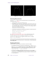
1.1 Making an Initial Scout Image
The following procedures outline all of the steps you need to take to begin using SEMS for
the first time. Some of the steps, such as pulse calibration, may not be necessary once you
have done them once. It is likely that in a real experimental session you may go through two
or more stages in defining the image orientation and position for the area of interest. We
call this final image the “target” image. But first, you will probably need to acquire an initial
“scout” image that can be used to accurately locate the target image.
01-999163-00 A0800
VNMR 6.1C User Guide: Imaging
17
Chapter 1. First Steps: Making an Image
Calibrating the Pulse Length
The first step is to calibrate the 90° pulse performance of the particular combination of
probe and sample, and to enter that information into the pulsecal database file:
• Use a simple pulse-acquire sequence (e.g, S2PUL), set the power level to intermediate
range (on newer UNITYINOVA or UNITYplus systems, set tpwr to about 50; on UNITY
or VXR-S systems, set tpwr closer to 90).
• Determine either the 90° or 180° pulse length (either value works for this procedure,
but a 180 is easier to determine and is generally not distorted by T1 relaxation).
Now, make an entry in the pulsecal file, as follows:
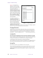
1.
Enter the command pulsecal.
If you have an entry in pulsecal, a table appears in the text window and the
following syntax message appears:
Usage: pulsecal(name,pattern,length,flip,power)
If you have not already made an entry in pulsecal, this message appears:
pulsecal file does not exist.
2.
Enter pulsecal again, this time supplying values for the arguments:
• For name, choose a name that makes sense for the probe and/or sample you are
using (if this is the cube phantom in the large imaging coil, for example,
'liccube' might make it easier to select the best entry again if you use this
combination at a later date).
• For pattern, unless you used a shaped pulse, enter 'square'. If you used
a shaped pulse, enter its name instead.
• For length, enter the pulse length, in µs.
• For flip, if it is a 90° pulse, enter 90, if it is a 180° pulse, enter 180, or
whatever value is appropriate.
• For power, enter a value in tpwr units used to measure this pulse length.
For example, if you measured a 180° pulse length of 800 µs with a tpwr of 80, your
entry is probably pulsecal('lic','square',800,180,80).
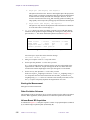
A listing of the new or updated pulsecal file is displayed in the text window. The
current date (month, day, year) is also included.
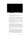
Determining the Reference Offset Frequency
You must provide the proton resonance offset frequency for an imaging experiment. You
can do this easily now while you have a proton spectrum readily available:
1.
Display one of the spectra in the array, for example, ds(1).
2.
Set the cursor on the resonance (probably water).
3.
Enter the command offset.
Record the number that appears in the message window.
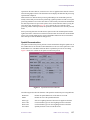
Retrieving the Parameter Set
Next, you must retrieve the parameter set to run the SEMS sequence.
1.
18
Join an available experiment. For example, to join experiment 6, enter jexp6.
VNMR 6.1C User Guide: Imaging
01-999163-00 A0800
1.1 Making an Initial Scout Image
2.
Retrieve the SEMS parameter set by entering the command sems.
You can also use the Files menu system to change to the system parlib directory
and load in the SEMS.PAR parameter set.
Most of the parameters that you need to know about and work with should now be
displayed. A few may require being set or selected, but the rest are computed for you.
Setting the rfcoil Parameter
The pulse calibration information, determined in “Calibrating the Pulse Length,” page 18,
is communicated to the system through the rfcoil parameter. The automated setup
routines use rfcoil to obtain information about probe performance from pulsecal and
to set pulse powers for the two rf pulses in SEMS.
• Set rfcoil='lic' (or use whatever name you chose for the pulsecal entry).
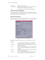
Setting the gcoil Parameter
An imaging spectrometer is often equipped with multiple gradient sets, which can be
interchanged for different sample sizes and experimental requirements. When a new
gradient set is introduced into the lab, a corresponding new calibration entry is required in
the directory /vnmr/imaging/gradtables. Such a calibration file should have been
created for any gradient set provided at initial system installation, so first check in the
gradtables directory for an entry appropriate for your system.
Because a gradient calibration file is a text file containing the maximum gradient strength,
rise time, and usable bore size for the gradient coil, a new file can be created manually with
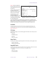
any text editor or, most easily, with the macro creategtable, as follows:
1.
On the VNMR command line, enter the command creategtable.
The following prompt appears:
Are all gradient axis calibrated to the same maximum
value? y/n
2.
If you respond y, you are asked to give a name to the file. Respond with:
• The letter m for a “main” gradient coil file name.
• The letter h for an “hpag” file name.
• The letter o if you want to define another name. If you respond with o, you are
asked to enter a name.
3.
Enter a brief description of the gradient coil to help in identifying this
gradtables entry in the future; for example,:
Main Actively Shielded Gradient
4.
Enter the usable bore size, in cm, for this gradient set. This value is used only as an
internal check of reasonableness for the field of view.
5.
Enter the maximum gradient strength, in gauss/cm, for the gradient set.
6.
Enter the rise time, in µs. Remember that Varian gradient hardware is installed with
a linear slew-rate limitation that is dependent on the gradient set.
The new gradient calibration is now ready to use, but first the configuration parameter
sysgcoil must be updated to reflect the hardware status.
1.
Enter the command setgcoil(file), where file is the appropriate
gradtables file name, for example, setgcoil('asg33').
01-999163-00 A0800
VNMR 6.1C User Guide: Imaging
19
Chapter 1. First Steps: Making an Image
This has the effect of setting sysgcoil to the same file name, but in this special
case, it also updates the configuration file as well.
2.
As new parameter sets are retrieved, and as other experiments are joined, the system
updates gradient calibration parameters to new values. To verify this, enter gmax?
and trise? to see that they have the correct values for your gradient hardware.
Note that gmax and trise are updated when a new parameter set is loaded, or when you
join a different experiment. One exception is joining an experiment that has gcoil
parameter set to the value of sysgcoil. If you update the gradient calibration parameters
of an already existing entry in gradtable, you must manually update gmax and trise
in the current experiment and others that have gcoil set to the sysgcoil value, or run
the macro _gcoil in each case.
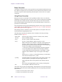
Setting the pilot Parameter
Some SEMS parameter sets might have not set the pilot parameter. To ensure that all of
the refocusing parameters are properly computed within the pulse sequence:
• Set pilot='y'
Setting the resto Parameter
The value of the resto parameter is used to make sure all positions are properly
referenced to the center of the magnet and gradients.
• Set resto to the value you found in “Determining the Reference Offset Frequency,”
page 18.
Setting the Field-of-View Parameters
Choose values for the image field-of-view (FOV) and enter them as follows:
1.
Set lro to the readout length, in cm.
2.
Set lpe to the phase encode length, in cm.
Do not use the old macros setgro and setgpe.
Setting the Slice Thickness
The parameter thk sets the slice thickness for an image.
• Set thk to the slice thickness, in mm. A value of 2 or 3 is a good place to start.
Selecting the Image Orientation
The parameter orient defines the imaging slice plane and indirectly controls a set of three
Euler angle parameters that the pulse sequence uses internally to achieve the desired
orientation. orient has allowed values of 'trans', 'sag', and 'cor', short for
transverse (Z slice gradient), sagittal (X slice gradient), and coronal (Y slice gradient),
respectively. A fourth entry of 'oblique' is also possible, but cannot be entered directly.
The entry for orient in the appendix (see page 324) describes oblique slice selection.
Because it is common for the sample to be fairly well centered on the X axis, even if it is
off center in Y and Z, you might start by entering orient='sag'. For a vertical bore
20
VNMR 6.1C User Guide: Imaging
01-999163-00 A0800
1.1 Making an Initial Scout Image
magnet, Z is more likely to be the on-center axis, so enter orient='trans'. This nearly
guarantees that you will slice through the sample without having to hunt around.
• Set orient to 'trans', 'sag', or 'cor', as appropriate.
Setting the pss Parameter
Parameter pss determines the slice position relative to the gradient origin. Setting pss
automatically sets the related parameter ns, the number of slices. You cannot set ns
directly, but entering an array of slice positions into pss results in an update of ns to the
proper value determined by the size of the pss array.
• Set pss as an array of slice positions, in cm, relative to the gradient origin (you
probably want to set pss=0).
Checking the seqcon Parameter
Some early SEMS parameter sets may have set the seqcon parameter to an incorrect
(although valid) setting. See “Acquisition Loop Control” on page 338 for more information
on this parameter. For proper multislice operation in SEMS:
• Check that seqcon='ncsnn'. Update it to this value if necessary.
Selecting Values for the tr and te Parameters
You may want to change the default values of tr and te. Keep in mind that unlike d1 in
the old IMAGE sequence, tr is now the correct measure of the total repetition time for a
multislice experiment (i.e., the time between successive excitations of one slice).
• If desired, set tr and te to new values, in seconds.
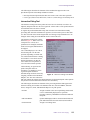
Entering the imprep Command
Everything necessary to set up an image is now done. To proceed:.
1.
Enter the command imprep.
This command takes the information about your rf coil, the slice thickness and field
of view you have selected, and computes and sets the parameters gro, gpe, gss,
tpwr1, tpwr2, and sw.
2.
If the parameter nv was zero, a warning is issued; otherwise, nv is left alone, so if
you want just a projection, first set nv to zero (nv controls the number of phaseencode steps, and is described in more detail on page 335) and ignore the warning.
3.
You should get the message “setup complete” if all went well. If not, you
should get an error message that gives you some hint of what could be wrong.
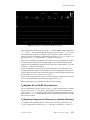
Checking the Readout Projection
It is a good idea to get a zero phase-encode projection to check proper operation and to
center the image in the readout direction.
1.
Enter nv=0 to specify just the projection, then enter ga to run the experiment.
2.
If the resulting projection is off-center, put the cursor where you want the new center
to be and enter movepro, which computes a new value for the pro (readout
position) parameter. pro sets the proper frequency during data acquisition.
01-999163-00 A0800
VNMR 6.1C User Guide: Imaging
21
Chapter 1. First Steps: Making an Image
Entering the go Command
The final step is to complete the image and see the end product.
1.
If you are making a projection with nv=0, enter ga; otherwise, for the complete
image, set nv to the number of phase encode increments you want (typically 128 or
256) and enter go (the difference is that ga automatically does a 1D transform of
every data line, which we don’t want, and go doesn’t).
2.
When the image is complete, enter ft2d to see the result.
Uncommonly Used Parameters
Although there is nearly a complete overlap in software between Varian’s horizontal
imaging, vertical microimaging, and standard analytical NMR systems, there are a few
parameters that are not normally used on a horizontal bore system. If set incorrectly, these
parameters can lead to artifacts or positional errors in images. It is therefore useful to check
the following parameters on horizontal bore imaging machines. Users with previous
experience with the SISCO 93.1 version of VNMR software are particularly advised to
learn about these parameters, because they did not exist in version 93.1.
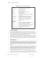
load
solvent
homo
Determines how shim values are updated, i.e., if they are obtained from the
software settings in the current experiment or from the actual existing
hardware settings. Most Varian users are familiar with this, but SISCO
users new to Varian software should refer to the VNMR Command and
Parameter Reference for more information.
Used to fine tune the spectrometer frequency to compensate for the small
reference field shifts caused by deuterium locking to different solvents.
Because most imaging experiments are performed without deuterium
lock, it is a good idea to set solvent='none' in all experiments,
including S2PUL, for consistent frequency settings. Failure to do this
results in an incorrectly referenced resto parameter, which in turn could
result in positional errors in images.
Enables time-shared homonuclear decoupling and should generally be set
to 'n' for imaging experiments.
1.2 Using the Scout Image to Plan a New Target Image
Now that you have acquired the first scout image, let’s use it to locate a new target image
that it includes whatever features you are interested in observing. You can skip many of the
steps we had to go through to get the scout, such as rf calibration, determination of resto,
etc., because these do not change from the scout to the new target image.
Moving the Parameters to New Experiment
You need to copy the parameter set you have been working with to another experiment (the
“target” experiment). You do not have to do this as the first step, but you need do it
eventually, so let's get it out of the way. It is possible to both plan and acquire the target
image in the same experiment, but then the scout image is lost, which we might want to use
again to plan a different target.
• To make the copy, enter mp(new_exp). This moves the entire imaging parameter set
to the designated experiment. For purposes of this example and the rest of this chapter,
22
VNMR 6.1C User Guide: Imaging
01-999163-00 A0800
1.2 Using the Scout Image to Plan a New Target Image
assume that you have been working in experiment 2 to acquire the scout image and
wish to use experiment 6 to acquire the target image. In this case, enter mp(6).
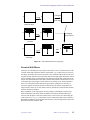
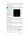
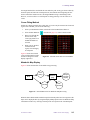
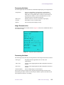
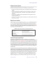
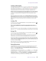
Starting the Planning Session
To start planning:
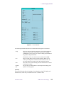
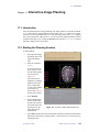
1.
Enter the command plan.
2.
Click on the Slice menu button.
3.
In the new row of menu buttons, click on Clear to remove any previous planning
information. The third button is now Mark 1.
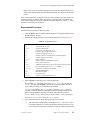
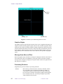
Marking the Target Slice Plane
To define a slice plane:
1.
Move the cursors to the first point you want to lie in the target image slice plane.
2.
Select the Mark 1 button.
3.
Move the cursors to the second point on the line that will define the slice plane.
4.
Select Mark 2.
You have just selected two points that describe a line through the current scout image. The
target image will be perpendicular to the scout slice plane, on the line you have defined.
Selecting Compute Target shows this.
If you decide you want to change one or both of the marked points, select Clear again and
follow the above procedure once more to define your new slice plane.
If you are working on a system that has gradient waveshaping capabilities, your slice plane
may lie at any angle. Slice planes that do not lie along one of the three major axes are said
to be oblique. If your system does not have gradient waveshaping, the gradient DAC
resolution is limited to 12 bits, which is in general not adequate to define arbitrary slice
planes with sufficient resolution in readout, phase encode, and slice select directions, and
so the software will at this point prevent you from continuing if you have defined a plane
that is oblique. (If you want to make sure your two points lie along one of the major axes,
here’s a hint: Move the cursors to the first point you want to mark; keep the mouse inside
the image boundaries but place the mouse arrow outside the blue image box to define the
second point. This method causes only one cursor to move and ensures that the two points
properly lie along one of the major orthogonal planes).
If you want to define a multislice experiment, you can use the ns and Gap buttons to specify
the number of slices and the gap between slices, respectively. When you compute the target
slice, the correct slice positions are entered into pss automatically. These slice positions
are defined in monotonic order, not in interleaved order. But unlike the older imaging
sequences, the slice order is not computed inside the sequence, but defined by the array
order of pss. You can enter the values of pss in any order that you like or use the macro
sliceorder to record slices automatically.
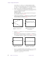
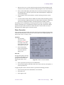
Computing and Displaying the New Target Parameters
At this point, you have specified the target imaging plane or planes on the scout image. You
now need to compute the new orientation and slice position for these planes:
• Select the Compute Target button
01-999163-00 A0800
VNMR 6.1C User Guide: Imaging
23
Chapter 1. First Steps: Making an Image
This button places the results in a set of “target” parameters that will be transferred in
the next step to the target experiment. You should see the target Euler angle values
printed in the message window, along with the slice position for the line you marked.
If you have defined a multislice target, you also see the slice positions displayed in the
text window at the bottom of the screen.
The newly defined slice position(s) are drawn over the scout image, allowing you to
visually verify that the target image(s) are properly aligned to pass through the desired
sample features.
If the new slice position is unsatisfactory, clear it and again perform the procedure (to
erase the old slice positions, select Redraw before Compute Target).
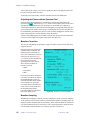
Transferring the Target Parameters
The new slice orientation and position parameters can now be communicated to the target
experiment. The parameters are the three Euler angles psi, phi, theta, the slice position
parameter pss, and slice thickness parameter thk. The parameter rfcoil is also
transferred, as well as resto, if both experiments have the same tn.
1.
Select the Transfer menu button.
This button displays a new menu of possible experiment choices and a descriptive
listing of each experiment in the text window (this same list can be created at any
time with the command explib2).
2.
Select the experiment to transfer to (in this case Exp 6).
If there is not enough space to show a menu button for each experiment, you might
not see a Current button (transfers internally to the current experiment) or an Other
button (enables you to type in an experiment number if the number you want is not
displayed).
Because we previously moved parameters from experiment 2 to 6, the target experiment is
the same in this case as the scout, except that we are changing the slice position and
orientation. We could just as well have transferred the new slice parameters to a completely
different imaging experiment (as long as it uses the same parameters to define slice position
and orientation).
At this point you are ready to start the new experiment. Because we have not changed the
field of view, slice thickness, or rf pulses, there is no need to execute imprep again. If you
decide to change any of these settings, just make sure you enter imprep again when
everything is adjusted the way you want it.
Checking the FOV and Entering the go Command
Before running the complete target image, it is generally a good idea to make sure that the
image is reasonably centered in the readout direction.
1.
Set nv=0, and then enter ga to get a projection and, if necessary, adjust the cursor
and enter movepro.
2.
Set nv back to the proper number of phase-encode steps, and enter go.
3.
When complete, ft2d shows you the new target image.
If you planned a multislice image, you have to set the cf parameter to select the slice
you want (remember, unlike old imaging sequences, the slices are in the order
specified by the pss array, and cf determines the array index). The macro dslice
displays up to 12 images at once from a multislice data set.
24
VNMR 6.1C User Guide: Imaging
01-999163-00 A0800
Chapter 2.
Imaging Experiments
Sections in this chapter:
• 2.1 “Basic Imaging Principles,” this page
• 2.2 “Time Domain to Spatial Domain Conversion,” page 26
• 2.3 “Slice Selection,” page 29
• 2.4 “Frequency Encoding,” page 32
• 2.5 “Phase Encoding,” page 34
• 2.6 “Image Resolution,” page 35
• 2.7 “Spatial Frame of Reference,” page 37
• 2.8 “Image Reconstruction,” page 38
• 2.9 “Important Imaging Parameters,” page 38
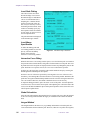
This chapter introduces the basic concepts necessary to understand MRI experiments. You
should be familiar with the terminology and principles in simple experiments in
conventional NMR because this chapter focuses on MRI-related topics. NMR concepts can
be easily understood when the process of a simple imaging experiment is analyzed. The 2D
spin-warp imaging sequence that is commonly performed in MRI is used in this chapter as
an example to illustrate principles and experimental aspects related to NMR.
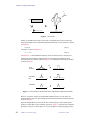
The spin-warp imaging sequence is based on the 2D Fourier transform principle for
converting the time domain NMR signals into image data. Most of the other imaging
techniques are also based on the Fourier transform idea and can be regarded as variations
of the spin-warp method.
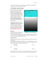
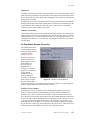
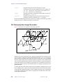
2.1 Basic Imaging Principles
This section contains a brief introduction to nuclear magnetic resonance imaging (NMRI),
magnetic resonance spectroscopy, chemical shift imaging, the 2D spin-warp imaging
sequence, and lists several additional references for more information about NMRI.
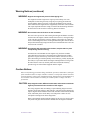
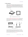
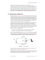
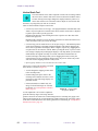
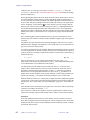
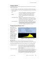
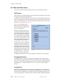
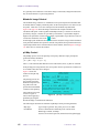
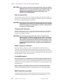
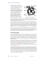
NMR Imaging
NMR imaging, or MRI, is used to obtain a map of the distribution of spins in a sample (for
example, protons in water). The inherent properties of the spins—such as spin density (T1,
T2, T2*), diffusion coefficient, etc.—affect the signal intensity in imaging experiments,
which makes the contrast in the resulting images easy to distinguish. This feature of
distinguishing different sample regions based on NMR-related properties makes imaging
an important tool in clinical, biological, and material sciences.
For example, clinical MRI scanning techniques are the preferred method for distinguishing
various soft tissues in the body. The spin density (T1 and T2) of water in different tissue
01-999163-00 A0800
VNMR 6.1C User Guide: Imaging
25
Chapter 2. Imaging Experiments
regions makes the contrast between tissues easy to distinguish. Experimental techniques
can be designed to further enhance the contrast between tissues. Special imaging
techniques can also be used to study flow, perfusion, diffusion, and susceptibility effects.
Methods for Obtaining Spectral and Spatial Information
Magnetic resonance spectroscopy (MRS) is the study of spectroscopic information in
different spatial regions in a sample. Volume-localized spectroscopic methods are used to
obtain spectral information from specific locations in a sample. Chemical shift imaging
(CSI) methods are another related class of experiments that are designed to provide both
spectral and spatial information from a single experiment.
2D Spin-Warp Imaging Sequence
2D spin-warp imaging is one of the simplest imaging sequences commonly used in NMRI.
Most of the other imaging sequences are variations of this fundamental sequence.
In “Basic Imaging Principles,” page 25, the basic principles of imaging are discussed based
on the spin-warp sequence. The information in that section is primarily meant to help a
novice grasp the basic principles and terminology of NMRI. The chapter contains a
description of the experimental aspects of NMRI so that you can understand the correlation
between the parameters and the resulting image. For a more theoretical understanding of
the imaging experiments, refer to any basic text or reviews on MRI.
References
The VNMR manual Getting Started contains more general information on operating Varian
spectrometers. Consult the manual VNMR Command and Parameter Reference for
additional information on VNMR commands or parameters.
2.2 Time Domain to Spatial Domain Conversion
As an example of Time domain to spatial domain conversion, consider a tube of water
inserted within an NMR probe and placed in the center of the magnet. The magnet produces
a homogeneous field in the region surrounding the water sample. A single pulse experiment
yields an NMR signal that, on Fourier transformation (FT), produces the frequency
spectrum of the sample, as shown in Figure 1.
Sample in a homogenous field, B0
Spectrum
rf
FT
t
FID
f0
Figure 1. Frequency Spectrum Produced by an NMR Signal
26
VNMR 6.1C User Guide: Imaging
01-999163-00 A0800
f
2.2 Time Domain to Spatial Domain Conversion
A single line at the resonance frequency, f0, is obtained. The frequency is defined by the
following Larmor equations:
f 0 = γ ′ ⋅ B0
[Eq. 1]
γ = 2π ⋅ γ′
[Eq. 2]
In Equation 1 and Equation 2, γ is the gyromagnetic ratio (rad.gauss-1sec-1) and B0 is the
magnetic field strength (gauss).
For protons, γ is 2.6752×104 rad.gauss-1 sec-1 and γ’ is 4257 Hz.gauss-1. In MRI, the
magnet strength, B0, is usually expressed in tesla (1 T = 10,000 gauss), whereas in
conventional NMR, magnet strength is commonly referred to in terms of the proton
resonance frequency in MHz.
The frequency spectrum that is displayed in NMR is referenced with respect to the
rf transmitter frequency. The center of the spectrum refers to the carrier frequency.
Therefore, spectral components that are above (positive) and below (negative) can be
measured by NMR. In MRI, the spatial-frequency components are measured with respect
to the resonance frequency of the major component in the sample, usually water. Therefore,
the carrier is placed on the water resonance frequency, f0, as part of the initial setup
procedure. Now, the center frequency in the spatial-frequency domain refers to the origin,
or the center, of the gradient frame of reference.
In addition to the standard equipment in NMR spectrometers, imaging systems are
equipped with X, Y, and Z field gradient coils that are designed to produce linear field
gradients along the x, y and z directions, respectively. In MRI, these field gradients are used
to get the spatial information from the sample. The x, y, and z gradient fields are orthogonal
to each other and their origins lie at the center of the gradient system. The field produced
in each direction is linear and ranges from a negative value to a positive value; the field at
the origin is zero.
Consider the water sample shown in Figure 1 and apply a linear field gradient along the y
direction, ranging from a negative value to a positive, as shown in Figure 2.
rf
FT
y
0
Gy
z
Gy
0
y
y
x
Sample in a field gradient
Magnetic frame of reference
Figure 2. Effect of a Field Gradient Along Direction y
In Figure 2, the field along the y direction is no longer constant but varies linearly,
depending on the position y. The field at a particular location, y, is defined by y.Gy, in which
Gy (in gauss/cm) refers to the field gradient along y direction. Therefore, the spins along
the y direction experience a unique field depending on the location of the y direction.
01-999163-00 A0800
VNMR 6.1C User Guide: Imaging
27
Chapter 2. Imaging Experiments
The frequency, fy, of the spins at various y locations is defined by the following equation:
fy = γ′ ⋅ ( B 0 + y ⋅ G y )
[Eq. 3]
In this equation, y refers to the y location (in cm) and Gy refers to the applied field gradient
(in gauss/cm).
Equation 3 is the most important equation in MRI because it correlates the spatial position
of the spins, y, to the measured parameter, fy. That is, the frequency spectrum measured is
a direct reflection of spatial information (along y) because, as shown in Equation 4,
fy ∝ γ
[Eq. 4]
when y=0, Equation 4 is the same as Equation 1 and Equation 2, so the frequency at the
origin of our frame of reference is equal to the resonance frequency of water, f0. It is
necessary to place the rf transmitter frequency at f0 so that images can be spatially
referenced with respect to the origin of our reference frame or the center of the magnet.
Under the previously
described conditions, a
single-pulse sequence
yields a spectrum that
contains a continuous
range of frequencies, as
shown in Figure 3.
Profile with a gradient on
Spatial-frequency spectrum
The frequency spread is a
direct reflection of the
0
0
spatial position of the
spins along the y
direction. Signal intensity
is directly related to the
amount of water at various
f0=0
0 f0
positions along y. The tube
Transmitter
Transmitter
of water appears as a
on-resonance
off-resonance
semicircle in the center of
the spectrum. The spatialFigure 3. Frequency Ranges
frequency spectrum,
shown in Figure 3, is also
referred to as a profile or
projection of the sample along the y direction.
y
The projection resolves the spatial-frequency components along a single direction. But an
imaging sample is three-dimensional, so more imaging must be done to visualize our
sample in 3D space. Many experiments have been designed in the past to uniquely identify
and map the spin distribution in the sample. Each experiment has its own advantages and
limitations. Experiments based on the spin-warp techniques are the most commonly used
in MRI. Therefore, it is useful to understand how these experiments resolve the spatialfrequency components of a 3D sample.
The 2D spin-warp experiment contains the following three parts, which correspond to the
preparation, evolution, and detection steps in a conventional 2D NMR experiment:
• Slice selection
• Phase encoding
• Readout
28
VNMR 6.1C User Guide: Imaging
01-999163-00 A0800
2.3 Slice Selection
2.3 Slice Selection
Magnetic resonance images are displayed as 2D pictures in either grayscale or color scale
for further analysis. The 2D images represent the NMR signals taken from a slice in the
sample, as shown in Figure 4. It is possible to selectively obtain signals from a slice by
using a slice-selection process. During the preparation phase of the experiment, only the
signals from a predetermined slice are pulsed so that only those excited spins contribute to
the resulting image. Slice selection involves using a selective rf pulse in combination with
a slice-selection gradient.
z
x
y
x
y
Slice selection
2D Image
Figure 4. 2D Image Resulting from a Slice Selection
The section “Time Domain to Spatial Domain Conversion,” page 26, described how the
presence of a field gradient causes a spatial frequency spread (profile) along the gradient
direction, shown in Figure 3. In the example shown in Figure 5, the profile along the
z direction is rectangular because the signal intensities from the sample at various points
along z are equal.
x
Gz
z
y
FT
rf
z
t
0
Figure 5. Rectangular Profile
The use of the hard pulse excites all of the spins in the sample because the excitation
bandwidth is wider than the frequency spread of the profile. However, if a soft, selective
pulse is used, a narrow bandwidth of the profile at the carrier frequency is excited. In other
words, spins corresponding to a narrow slice at z= 0 are selectively excited. The resulting
profile, referred to as the slice profile, is shown in Figure 6.
01-999163-00 A0800
VNMR 6.1C User Guide: Imaging
29
Chapter 2. Imaging Experiments
x
z
y
Gz
rf
z
0
Figure 6. Slice Profile
Ideally, a rectangular slice profile is preferred. A rectangular profile can be achieved by
using a shaped pulse with its amplitude modulated in the form of a sinc function, as shown
in Equation 5:
sin ( θ ) ⁄ θ
[Eq. 5]
The phase θ is given in Equation 6:
θ = 2 π vt
[Eq. 6]
Ιn Equation 6, v is the modulation frequency of the sinc function and t is the time axis.
Theoretically, the resulting excitation profile can be predicted by taking the Fourier
transform of the sinc function, which in Equation 5 is rectangular in the frequency domain,
as shown in Figure 7.
FT
Sinc
function
t
f
Truncated
sinc
t
f
t
f
Gaussian
Figure 7. Sinc Function, Truncated Sinc Pulse, and Gaussian-Shaped Slice Profiles
However, in practice, because of experimental limitations such as T2*, the pulses are
limited to about 4 ms or less. The resulting truncated sinc function has an excitation profile,
as shown in Figure 7.
Gaussian-shaped pulses are also used for slice-selection purposes. The Gaussian pulse
produces a profile that is also a Gaussian, as shown in Figure 7. In general, this simplified
approach is only true for short (about 30o or less) flip angles. At larger flip angles, pulses
30
VNMR 6.1C User Guide: Imaging
01-999163-00 A0800
2.3 Slice Selection
show large behavior that is not ideal because of the nonlinear response of the NMR spins.
The pulse shapes can be optimized to produce more ideal pulse characteristic for specific
applications. For example, the rf pulses can be optimized by computer-iterative procedures
to give slice profiles that are closer to rectangular shape. Such pulses minimize
contamination of the image from regions outside the slice region of interest. The
optimization procedures can also produce pulses that are closer to ideal in terms of flip
angle and phase response across the slice profile.
So far, we have assumed the transmitter
frequency is on-resonance, which
corresponds to a slice plane at z = 0. It
is also possible to excite a slice at any
location along the slice direction by
changing the rf transmitter frequency
during the excitation phase of the
experiment, as shown in Figure 8.
For offset slice selection, the
transmitter offset frequency depends on
the amplitude of the slice gradient that
is applied and is defined by the
following equation:
( fs – f 0 ) = γ′ d ⋅ gss
[Eq. 7]
In this equation, fs is the transmitter
frequency (in Hz) that is needed to
excite a slice at distance d (in cm) from
the origin, f0 is the resonance frequency
(in Hz) of water, and Gss is the sliceselect gradient (in gauss/cm).
Slice 1
Slice 2
Slice 3
0
z
Figure 8. Multislice Excitation
Note: You must return the transmitter reference frequency to the original position during
the detection stage of the experiment for proper referencing of the resulting profile.
Slice thickness is directly related to the bandwidth of the excitation pulse. For a sinc pulse,
the excitation bandwidth w (in Hz) is defined by the following equation:
w = 2⁄λ
[Eq. 8]
In Equation 8, λ refers to the wavelength (in sec) of the sinc pulse.
The slice thickness parameter is dependent on the slice gradient because the slice gradient
affects the frequency spread or the profile along the slice direction. Equation 9 represents
the relationship between the band width of the rf pulse w (in Hz), slice gradient Gss (in
gauss/cm), and slice thickness st (in cm).
w = γ ′ ⋅ Gss ⋅ st
[Eq. 9]
The presence of a slice gradient during the slice-selection pulse has an undesirable effect
on the signal. The signals lose phase coherence, which results in a rapid signal loss. This
signal loss can be restored by applying a gradient of opposite sign, as shown in Figure 9.
The amplitude of the slice rephasing gradient, Gsd, can be obtained by the following
equation:
t4
k ∫ gss ⋅ dt =
t7
01-999163-00 A0800
t7
[Eq. 10]
∫ gss ⋅ dt
t4
VNMR 6.1C User Guide: Imaging
31
Chapter 2. Imaging Experiments
Slice refocusing gradient
rf
t4
Gss
t5
t1
t2
t2'
t7
t6
t3
Figure 9. Signal Loss Restoration
In Equation 10, the factor k is approximately equal to 1. Equation 10 simply means that the
shaded areas in Figure 9 must be approximately equal for maximum refocusing of the spins
after the slice-selection pulse.
Some experimental macros and parameters in VNMR related to slice selection are listed in
Table 1. For more information on VNMR macros, parameters, and commands, refer to the
manual VNMR Command and Parameter Reference.
Table 1. Experimental Macros and Parameters
Macro
Function
plan
Displays a menu that provides access to the target scan plan utilities. plan
allows users to define slice positions, offsets gap, and the number of slices
by using a graphical tool. The parameters can then be transferred to a target
experiment using the transfer macro.
Parameter
Function
ns
Sets the number of slices to be acquired for multislice sequences.
pss
The position of slice offset, in cm. pss is an arrayed parameter; therefore,
an arbitrary number of slices can be directly entered. A more convenient
way to enter slice offset parameters is to use the plan macro.
resto
NMR resonance offset frequency, in Hz.
thk
The slice thickness, in mm.
2.4 Frequency Encoding
In the presence of a readout gradient, the spatial-frequency components can be directly
visualized by observing the profiles along that direction. Even though the presence of a
readout gradient during the FID signal gives the necessary information, in practice it is
desirable to collect an echo signal. The echo signal, when Fourier transformed, generates
only absorption components in the resulting spatial-frequency spectrum or profile. The
broad dispersive components are cancelled because of the symmetry of the echo signal.
The cancellation of dispersive components is a big advantage when dealing with imaging
data because the image or profile can be generated by simply calculating the absolute value
without the need for any phase correction. An echo signal can be generated by first
32
VNMR 6.1C User Guide: Imaging
01-999163-00 A0800
2.4 Frequency Encoding
dephasing the excited spins by using a readout gradient pulse and then rephasing the spins
by reversing the sign of the gradient. When the area of the rephasing gradient equals the
area of the dephasing gradient, a “gradient echo” is formed, as shown in Figure 10.
tr
te
rf
gss
Refocusing gradient
at
t4 t5
gro
t6 t7
t8 t9
t9'
at/
t10 t11
Dephasing gradient
ADC
Gradient echo
Figure 10. Readout Gradient and Gradient Echo
The readout gradient is applied during the acquisition time, at, so that the echo appears at
the center of the acquisition window, a condition that is assured if the shaded areas in Figure
10 are equal, as shown in the following equation:
t4
∫ gro dt
t6
=
t3
[Eq. 11]
∫ gro dt
t5
The Fourier transform of the echo signal gives the profile along the readout direction; only
the signal from the selected slice contributes to the profile. The sequence shown in Figure
10 is commonly used to observe the profile during the initial setup of imaging experiments.
The profile can be very useful in doing the following procedures:
• Positioning the sample along the readout direction.
• Checking or calibrating the rf pulse power.
• Setting the receiver gain.
• Checking the signal-to-noise ratio.
• Optimizing the pulse sequence parameters such as te and tr.
Readout gradient strength determines the frequency spread of image components in a
profile. Therefore, the spectral width must be sufficiently wide to resolve all the spatialfrequency components along the readout direction. Otherwise, frequency components
outside the spectral window cause “fold-over” artifacts.
The readout gradient and spectral width determine the field of view along the readout
dimension, defined by the following equation:
sw = γ′ ⋅ gro ⋅ lro
01-999163-00 A0800
[Eq. 12]
VNMR 6.1C User Guide: Imaging
33
Chapter 2. Imaging Experiments
In Equation 12, gro (in gauss/cm) is the readout gradient, lro is the field of view along
the readout dimension (in cm), and sw is the spectral width or bandwidth (in Hz). The
spectral width is related to the acquisition parameters, defined by the following equation:
sw = ( np ⁄ 2 ) ⁄ at
[Eq. 13]
In Equation 13, np is the total number of (real plus imaginary) points digitized, and at is
the acquisition time (in sec). The maximum bandwidth, sw, is determined by the digitizer
used on the system. A typical 16-bit digitizer, used on most imaging systems allows a
spectral bandwidth limit of 500 KHz, whereas some 12-bit digitizers, used in solids NMR
systems, allow a maximum bandwidth of 5 MHz. The parameter np is usually set to
approximately 128 or 256.
2.5 Phase Encoding
During slice selection (the preparation phase of an experiment), it was possible to restrict
the signals to a plane. Spatial-frequency distribution in a plane is achieved by using the
evolution (phase encoding) and detection (readout) phases of a 2D NMR experiment. In a
spin-warp imaging experiment, a 2D dataset is collected and each orthogonal dimension
contains information about the phase encode and readout dimensions, respectively.
Slice selection and frequency
encoding (detection phase) are
rf
easily visualized by viewing
the slice profiles and readout
gss
profiles, shown in Figure 5 and
Figure 11. The concept of
phase encoding is less obvious
gro
because information is
t5
t6
preserved in the second
t7
t4
dimension as a phase
gpe
modulation. Fourier
transformation along the
ADC
second dimension provides
spatial-frequency information.
Spatial information
Figure 11. Gradient Echo Imaging Sequence
corresponding to the phase
dimension is encoded by the
use of a gradient pulse during phase encoding, as shown in Figure 11.
For example, consider a spin at a specific location, y (in cm), along the phase encode
dimension. The phase of the spin, φ, is affected by the phase encoding gradient amplitude,
gpe, and its duration, tpe. For an arbitrary pulse, the phase is proportional to the integral
area of the gradient pulse, defined by the following equation:
t7
φ =
∫ γ ⋅ y ⋅ gpe ⋅ dt
[Eq. 14]
t4
In this equation, φ is the phase in radians. For a square pulse, Figure 14 reduces to the
following expression:
φ = γ ⋅ y ⋅ gpe ⋅ tpe
[Eq. 15]
In Equation 15, tpe is the phase encode time (in sec).
34
VNMR 6.1C User Guide: Imaging
01-999163-00 A0800
2.6 Image Resolution
From Equation 15, it is clear that either tpe or gpe can influence the phase of the resulting
NMR signal. In the spin-warp experiment, the phase encode gradient is varied (rather than
the phase encode time) from scan to scan in a stepwise manner. Therefore, the phase of the
spins at location y are phase-modulated in a predictable linear fashion. The modulation
frequency is directly proportional to the spatial location y. Fourier transformation along the
phase encoding direction converts the time domain and phase modulation into spatialfrequency domain.
The field of view along the phase encode dimension is related to the gradient step size.
Therefore, it is convenient to define the parameter pestep, which is equal to the
incremental area of the phase encode gradient pulse, defined by the following equation:
t7
pestep =
∫ gpe ⋅ dt
[Eq. 16]
t4
The number of 2D phase encode steps to be acquired is determined by the parameter nv.
nv experiments are run when the phase encode gradients are set to the values, defined by
the following equation:
pestep ⋅ ( n – ( nv + 1 ) ⁄ 2 )
[Eq. 17]
In Equation 17, n = 1, 2, 3,... nv. Equation 17 ensures an equal number of positive and
negative phase encode gradients are applied during the phase encode time tpe. For
example, if nv = 4, the gradient amplitudes are stepped in half-integral units of
−1.5, −0.5, +0.5, +1.5
The phase-modulated nature of the imaging experiment would normally produce unwanted
dispersion components in the final image. This problem is avoided by phase encoding with
both positive and negative values of the gradient to create a pseudo-echo signal along the
phase encode dimension that is transformed with pure absorption components. Therefore,
as in the case of the gradient echo signal, an absolute value calculation yields an image
without the need for any phase correction.
The field of view along the phase dimension is related to the step size of the phase encode
gradient and is defined by the following equation:
lpe = l ⁄ ( γ′ ⋅ pestep )
[Eq. 18]
In Equation 18, lpe is the field of view along the phase encode dimension, in cm.
It is important to choose the parameters so that the field of view, lpe, is greater than the
spatial frequency spread along the phase encode dimension, or else the spatial components
that lie outside the field of view will cause fold-over artifacts.
2.6 Image Resolution
Image resolution defines the ability to separate the signal arising from adjacent regions in
the object being imaged. Decreasing the resolution improves the appearance of the actual
shapes of the separate parts of an object. An image is displayed as a 2D digitized picture
and each digital element is referred to as a pixel (or picture element). In the case of a 3D
image, each digital element is referred to as a voxel (or volume element).
Resolution of an image depends on two factors:
• Frequency spread over the field of view, which is determined by gradient strengths
gpe and gro.
• Pixel size, which is determined by the number of complex data points in the readout
dimension, np/2, and the number of phase encode steps, nv.
01-999163-00 A0800
VNMR 6.1C User Guide: Imaging
35
Chapter 2. Imaging Experiments
Minimum resolution is determined by linewidth, which determines whether the signal from
one region can be confined to a single pixel. Linewidth is mainly determined by spin-spin
relaxation time and also susceptibility and inhomogeneity at a specific location in the
sample.
Resolution along the phase encode dimension is defined in the following equation:
[Eq. 19]
Rpe = lpe ⁄ nv
Similarly, resolution along the readout dimension is defined by the following equation:
Rro = lro ⁄ ( np ⁄ 2 )
[Eq. 20]
To illustrate image resolution, assume the image is from a sample consisting of three
spheres filled with water, as shown in Figure 12.
Water
Pixel size
ni=np/2=8
Pixel size
ni=np/2=16
Pixel size
ni=np/2=32
Figure 12. Image Resolution of Three Water-Filled Spheres
When the number of data points is small, one pixel can contain both a large region that does
give an NMR signal and a large region that does not give an NMR signal. The lack of NMR
signal causes the edges of the object to be poorly defined and can cause overlap between
adjacent structures so that the separate objects cannot be distinguished from one another.
As the number of data points (and/or gradient frequency spread) is increased, the signal
from any given point is better able to be confined to a single pixel, so the amount of overlap
between adjacent structures diminishes and the image is better defined.
The usual number of chosen data points is 128 or 256. A smaller number results in
insufficient resolution and can also cause artifacts created by truncation of the time domain
36
VNMR 6.1C User Guide: Imaging
01-999163-00 A0800
2.7 Spatial Frame of Reference
signal. A larger number of points along the phase encode dimension (ni or nv)
significantly increases the data acquisition times. More points along the readout dimension
increase the acquisition; therefore, the echo times are increased, which leads to loss of
signal caused by the T2* effect. The number of data points is usually set to a power of 2, as
required by the Fourier transform. Sometimes image presentation can be improved by zerofilling, that is, by increasing the number of image points along the phase and readout
dimensions. However, this method does not improve the inherent resolution of the image.
2.7 Spatial Frame of Reference
The section “Image Resolution,” page 35, described the NMR method for resolving the
spatial dimension along a particular direction. In reality, a sample is a three-dimensional
(3D) object. Therefore, it is necessary to be able to resolve the spatial information in 3D
space. It is convenient to define a frame of reference for dealing with a 3D sample. The
orientation of the magnetic fields produced by the gradient coils inside the magnet defines
a coordinate system for imaging experiments. An understanding of the workings of this
coordinate system will help you to operate the imaging instrument.
The origin of the whole system lies at the center of the magnet, which is also the center of
the gradient coil system. Gradients produce a zero field in the center of the magnet.
Therefore, the frequency associated with the origin or magnet center is the resonance
frequency for the particular nuclear substance intended for imaging. For example, water is
the chemical substance most often imaged for the proton, and the frequency at the origin of
the gradient reference frame puts the NMR signal from water “on-resonance.”
There are two types of imaging magnets:
• Narrow bore, vertical magnets, which are used for MRI microscopy (MRM)
• Wide-bore, horizontal, magnets, which are used for larger samples
In the case of horizontal magnets, shown in Figure 13, the z axis is defined as being in the
direction along the bore of the magnet, going from the cable end (back) of the magnet to
the sample end (front) of the magnet. The x and y directions in the horizontal magnets and
refer to the left-right and top-bottom orientations respectively, as shown in Figure 13.
(Top) Supine
y
Front
Back
Right
Left
x
z
(Bottom) Prone
Figure 13. Horizontal Magnet
However the x and y directions in vertical bore magnets are less obvious because of the
cylindrical symmetry of those magnets, shown in Figure 14.
During installation, the gradient coils and shim coils are aligned and fixed so that they are
symmetrical with respect to the center of the magnet. For imaging, you must place the rf
coil in the magnet center and position the sample within the rf coil.
01-999163-00 A0800
VNMR 6.1C User Guide: Imaging
37
Chapter 2. Imaging Experiments
The image planes are referenced with
respect to the gradient frame of reference.
The three commonly referenced planes
are sagittal, coronal, and transverse and
they respectively refer to the planes that
are perpendicular to the x, y, and z axes, as
shown in Figure 14. Images can also be
obtained from arbitrary, or oblique,
planes. The plan macro in VNMR
allows you to define oblique planes by
using a graphical tool and a reference
image. For some applications, you might
want to collect a 3D volume image instead
of a 2D slice image. For a 3D volume
image, it is possible to analyze or view the
data by using 3D image analysis routines.
Top
x
y
z
Bottom
Figure 14. Vertical Magnet
2.8 Image Reconstruction
The imaging data is collected as a 2D arrayed time domain signal, S(t1, t2), in which t1
and t2 respectively refer to the phase encoding and readout dimensions. (For historic
reasons, in conventional 2D NMR, the subscript numerals 1 and 2 respectively refer to the
phase encoding and detection dimensions.)
When the signals are viewed along either the phase encode or readout dimension, the time
domain signals take the form of an echo signal. Fourier transformation (with respect to t1
and t2 using the ft2d routine) yields the spatial-frequency data, S(F1, F2). The symmetry
properties of the echo signal yields only absorption-mode components in the dataset, S(F1,
F2), without any undesirable dispersion mode components. The yield of only absorptionmode components is a significant advantage in imaging because the final image can be
obtained by simply taking the absolute value spectrum, |S(F1, F2)|, without the need for any
phase correction.
The appearance of the image can be improved or modified by digital filtering. Filter
functions can either be applied in the time domain or the spatial domain. In the case of time
domain data, t=0, point is in the center of the time axis. Therefore, an apodization function
symmetrical to t=0 should be applied. For example, a gaussian (“shifted”) function has the
effect of improving the SNR of the resulting image at the expense of loss of resolution
(“blurring”) of the image. Another common way to improve the image appearance is to
interpolate the image during the display process. Interpolation is also equivalent to zerofilling the data in the time domain.
2.9 Important Imaging Parameters
This section describes three important timing parameters—tr, te, and ti—that are used
during the performance of imaging experiments.
tr, Recycle Time
The tr parameter defines the time between the beginning of one scan and the next.
38
VNMR 6.1C User Guide: Imaging
01-999163-00 A0800
2.9 Important Imaging Parameters
It is important to allow sufficient recycling time so that the excited spins have sufficient
time to return to equilibrium. In the case of a 90° excitation pulse, a recycle time of >4.T1
must be allowed. If the recycle time is too short, the signal gets saturated, which results in
a gradual loss of signal intensity, eventually reaching an equilibrium or steady-state
condition. However, this T1-dependent signal variation can be exploited to enhance T1
contrast in the images.
In experiments involving quantitative work
such as relaxation studies and pulse power
and receiver gain calibration, tr must be
set to greater than 4.T1 to avoid erroneous
results. In experiments such as FLASH, the
flip angle is set to approximately
5° ∞∞to 30° and tr is set to small values
(about 10 µsec to 50 µsec) so that the
images can be acquired very rapidly. Table
2 lists the approximate relaxation times, at
4.7 T, of some commonly used liquids.
Table 2. Relaxation Times
Liquid
Time
Doped water (1 g CuS04/liter)
0.6 s
Vegetable oil
0.3 s
Tap water
3s
Degassed distilled water
26 s
te, Echo Time
Unlike in conventional NMR spectroscopy, imaging experiments usually generate either
gradient- or spin-echo signals. The resulting signal intensity therefore depends on the echo
time, te. Echo time is the time between the center of the rf excitation pulse and the position
of the echo maximum, as shown in Figure 15.
Signal decay caused by T2*
90
180
180
180
180
Echo maxima decay caused by T2
Figure 15. Signal Intensity
Echo time delay results in some loss in signal because of spin dephasing, which is caused
by T2* effects. T2* is defined as a combination of spin-spin relaxation (T2), magnetic field
inhomogeneity, and susceptibility effects. Susceptibility effects are caused by interactions
of the magnetic field with the heterogeneous sample, which produces localized field
gradients within the sample. T2* effects tend to get worse at higher fields. Signal loss
caused by T2* effects is exponential. Therefore, at long te values, a dramatic loss of signal
intensity can result, leading to degradation of image quality.
It is therefore advantageous and sometimes even necessary to shorten the te value to
improve image quality. However, there is a limit to the minimum te because echo time
depends on the acquisition time and the rf and gradient pulse delays in the sequence. The
shortest, achievable echo time depends mainly on maximum gradient performances such as
maximum gradient strengths, rise times and residual eddy currents. However, te delay can
also be used to enhance the T2 or T2* contrast in images. For example, in functional MRI,
brain activity causes localized susceptibility in the brain, which is enhanced by using the
01-999163-00 A0800
VNMR 6.1C User Guide: Imaging
39
Chapter 2. Imaging Experiments
gradient echo imaging techniques. The T2* effects of solid materials are very short (<100
µs), so special experimental techniques need to be used to obtain images from such
samples.
ti, Inversion Time
ti is an important contrast parameter in imaging. The inversion time contrast between
different components in the sample can be enhanced by performing a ti inversion recovery
sequence (ti ir).
The ti ir imaging sequence involves applying a 180° inversion pulse and a delay, ti, at
the beginning of a conventional imaging sequence. The inversion pulse flips the
magnetization to the z direction. The spins return to equilibrium, exponentially, with a time
constant inversion time, as illustrated in Figure 16.
180°
Exponential recovery
of the longitudinal
magnetization
t
0
tnull=0.69T1
Figure 16. Equilibrium Magnetization
Sampling the magnetization after the inversion time delay results in varying signal
intensities, depending on the ti of the spins. Notice that the signal is negative at short
inversion times and gradually becomes positive at longer inversion times. When
ti=(0.69.T1), the signal is zero, as shown in Figure 16. If the sign of the intensities is
to be retained in the images, it is necessary to phase correct the images instead of taking the
absolute value mode. ti ir imaging experiments can be inefficient because of the long
recycle time required to allow the spins to return to equilibrium.
40
VNMR 6.1C User Guide: Imaging
01-999163-00 A0800
Chapter 3.
Imaging Pulse Sequences
Sections in this chapter:
• 3.1 “Initial Setup,” this page
• 3.2 “Conditions for Use,” page 42
• 3.3 “GEMS Multislice Imaging,” page 44
• 3.4 “Obtaining a GEMS Image,” page 49
• 3.5 “Echo Planar Imaging and Phase Correction Map Files,” page 51
• 3.6 “Commands, Macros, and Parameters,” page 62
This chapter describes some pulse sequences for imaging available on Varian NMR
spectrometers. You should be familiar with basic operations of the spectrometer; therefore,
explanations of operations such as shimming and tuning are not included in this chapter.
Refer to the manual Getting Started and the VNMR User Guides for more information on
various spectrometer operations. More detailed descriptions of all commands, macros, and
parameters are in the appendix, “Commands, Macros, and Parameters,” of this manual and
in the manual VNMR Command and Parameter Reference.
3.1 Initial Setup
This section describes the procedure for initially setting up imaging experiments using a
single-pulse sequence.
The main purpose of the initial setup procedure is to make sure that the system is properly
functioning and to determine the rf calibration parameters. Once the initial setup has been
completed, the rf calibration parameters, such as transmitter frequency and power, can be
used for subsequent imaging experiments and therefore do not need to be repeated.
However, if the sample or coil is changed, it might be necessary to repeat the initial setup
procedure.
Table 5 on page 62 summarizes the commands, macros, and parameters that are used.
1.
Position the sample in the magnet.
Because imaging coils and samples come in various sizes and shapes, it is important
to position the sample and the rf coil in the center of the magnet.
2.
Place the sample in the magnet and tune the probe.
Be aware that different imaging samples can influence the tuning of the probe,
depending on their sizes, compositions or even the positioning within the rf probe.
3.
Use the single pulse sequence s2pul to check for the NMR signal. Initially use a
sufficiently wide spectral bandwidth to avoid aliasing of the proton signal.
The spuls macro can be used to load the default parameters suitable for imaging
rather than for high resolution spectroscopy.
01-999163-00 A0800
VNMR 6.1C User Guide: Imaging
41
Chapter 3. Imaging Pulse Sequences
4.
Shim, if necessary.
Unlike high-resolution spectroscopy, shimming is not critical for most imaging
experiments. Even when the linewidths are 50 Hz to a few hundred hertz, good
images can be obtained. Typical linewidths for imaging samples such as plant and
animal tissues are about 50 Hz to 150 Hz. However, improved field homogeneity can
produce better results. Good magnet homogeneity is critical for some experiments,
such as echo planar imaging (EPI), gradient echo, multislice imaging (GEMS), and
spectroscopic imaging.
5.
Use the s2pul sequence to set the transmitter frequency on resonance.
The transmitter offset frequency parameter, tof, is needed to define the spatial
reference position (the center of the magnet and gradient coils). The macro setof
automatically determines the spatial reference position using the tallest peak in the
spectrum. The offset frequency is then stored in the file $HOME/vnmrsys/
H1offset. (When running imaging sequences, the macro ldof sets the imaging
reference frequency parameter, resto, to the value saved in the H1offset file.)
On vertical bore systems, the Z0 shim (B0 field) can be adjusted so that the
transmitter frequency is on the peak of interest (usually water); in which case, tof
and resto parameters are usually set to 0.
The offset macro can be used to determine the frequency offset corresponding to
the cursor location. The movetof macro can be used to set the transmitter
frequency (tof) to the cursor position.
6.
Calibrate the pulse power. Measure the 90° or 180° pulse and enter it into the
pulsecal database.
The setarray macro can be used to set up an array of pulse width values for the
calibration experiment. The macro ga collects and displays the Fourier-transformed
data. The command dssh allows you to display the arrayed spectra.
The findpw macro lets you more conveniently calibrate the pulse powers. findpw
automatically determines the maximum and minimum signal from a set of ten,
predefined pulse lengths and enters the calibration values into the pulsecal
database. Once the pulse power is calibrated, pulse parameters such as pulse width
(pw) and shape (e.g., pwpat) in imaging pulse sequences can be easily changed.
Pulse powers are automatically computed by the imprep routine. Different
imaging samples can affect the tuning (Q) of the imaging coil. Therefore, it is
necessary to calibrate the pulse with each sample so that the proper pulse powers are
calculated for the imaging sequences.
3.2 Conditions for Use
This section lists the conditions that are necessary to use imaging pulse sequences, and
information on the lock and spin parameters and the spuls and s2puls macros.
Receiver Gain Adjusted
Imaging samples generally produce excessive NMR signals that often saturate the receiver.
If the ADC overload error message is displayed, you must set the gain to a lower value. It
might also be necessary to further attenuate the incoming signal by manually setting a
signal attenuator or by setting the parameter presig='l' to presig='h'. The macro
setgn automatically sets the receiver gain, based on the input signal.
42
VNMR 6.1C User Guide: Imaging
01-999163-00 A0800
3.2 Conditions for Use
Recycle Time Adjusted
When setting gain or measuring pulse power, you must increase the predelay parameter
(d1) or recycle time parameter (tr) to greater than 4*T1 to allow the spins to return to
equilibrium before subsequent rf pulses.
Lock, Spinner, Decoupler Commands and Parameters Disabled
If you use a spectrometer that is also used for high-resolution spectroscopy, make sure that
the commands and parameters relevant to the lock, spinner, and decoupler are disabled. The
commands and parameters are disabled when they have the following settings:
homo='n'
lock='u'
lockpower=0
spin=0
spin='n'
The spuls macro is convenient for loading s2pul pulse sequence parameters for
imaging systems. (The s2pul macro is used in high-resolution spectroscopy and might
incorrectly initialize the parameters for imaging.)
Pulse Power Set Low
Imaging spectrometers are usually equipped with high-power rf amplifiers. Make sure that
the pulse power is set sufficiently low to avoid any damage to the rf coil.
Gradient Calibration File Created
Imaging systems can be equipped with either a single gradient coil or multiple gradient
coils. The gradient calibration information, or file, corresponding to each coil must exist in
the /vnmr/imaging/gradtables directory. Use the creategtable macro to
create the gradient calibration file.
Gradient Amplifier On
The gradient amplifier must be turned on and enabled before proceeding with the initial
setup procedure. Be aware that x, y, and z shimming is done via the gradient coils and that
the amplifiers can generate a small dc offset current that must be corrected by shimming.
Eddy Current Compensation Files Loaded
If you have a microimaging system with the computer-controlled analog eddy current
compensation, use the program ecctool to load the appropriate file. For systems equipped
with digital eddy current compensation (DECC), use the decctool program, described in
Chapter 8, “Digital Eddy Current Compensation,” to load the appropriate file.
Shim Power Supply Turned On
The shim power supply must be turned on for shimming purposes during experiments. If
the shim currents are high, they can generate excessive heat in the bore of the magnet. Air
or water cooling is employed to remove the excess heat buildup in the magnet. If the system
is not being used for extensive periods or if the air or water cooling is turned off, turn off
the shim power supply.
01-999163-00 A0800
VNMR 6.1C User Guide: Imaging
43
Chapter 3. Imaging Pulse Sequences
Pulse Calibration Done
Imaging sequences expect the rf calibration information to be present in the pulsecal
database. The rfcoil parameter must be initialized to the entry in the pulsecal
database.
Air or Water Cooling Turned On
Air or water cooling systems must be enabled for gradient experiments. Cooling is
necessary to remove the heat buildup in the bore of the magnet caused by the gradient and
shim coils. Gradients systems are usually equipped with protection devices to detect and
shut down the amplifier in the absence of either air or water flow.
3.3 GEMS Multislice Imaging
This section describes the steps involved in setting up experiments and collecting imaging
data using the gradient recalled echo sequence, which is also known as FLASHTM or
GRASSTM. Because the setup procedure for most imaging experiments is similar to that of
the GEMS sequence, read this section before proceeding to other imaging sequences.
Requirements
Your system must be configured for imaging, and gradient calibration and eddy current
compensation procedures must have been completed. Gradient calibration and eddy current
compensation are usually done during installation of the system, so you do not need to
repeat those procedures. If those procedures have not been done, contact your system
administrator.
Description
GEMS is essentially the same as the 2D spin-warp sequence described in “Basic Imaging
Principles,” page 25. GEMS uses the Fourier transform principle to convert 2D time
domain signals to a spatial-frequency domain (image). Most of the other commonly-used
imaging sequences can be regarded as variations of this basic sequence. GEMS uses a
single excitation pulse; therefore, the pulse flip angle can be reduced at the expense of
signal-to-noise ratio. The main advantage of using a smaller flip angle is that the sequence
can be rapidly repeated using a shorter repetition time (tr). This advantage enables you to
obtain images in about one second.
Imaging Sequence
The initial excitation pulse is a slice-selection pulse designed to excite a specific slice in an
object. The slice offset is specified by the parameter pss (in cm) and its thickness, by the
parameter thk (in mm). The flip angle of the excitation pulse is usually set to about 5° to
30° so that each scan can be rapidly repeated with a short recycle time (tr). Because
rapidly repeated scanning is an important feature of the GEMS sequence, it is commonly
used in situations in which rapid image acquisition is the primary goal.
For a gradient echo to be generated by the read gradient, the signal must first be dephased
and then rephased, as shown in Figure 17. The Fourier transform (ft) of the echo signal
yields a profile along the readout direction. During the initial setup process, you can view
the echo and its profile by setting the number of phase encode steps, nv, to 0. The profile
44
VNMR 6.1C User Guide: Imaging
01-999163-00 A0800
3.3 GEMS Multislice Imaging
can be used to position the sample (along the readout direction) in the magnet. It can also
be used for pulse calibration and for setting the receiver gain.
tr
te
rf
gss
gro
gpe
ADC
Figure 17. Gradient Echo Imaging Sequence
Data Collection
Set nv, the number (64 or 128) of phase encode steps, before entering go to acquire the
image. For efficiency, the GEMS sequence collects the data in a compressed format
(seqcon='nscnn').
If the data is collected in the standard (noncompressed) format (seqcon='nssnn'), the
overhead in the end-of-scan operation can influence the true recycle time in the pulse
sequence. This situation is particularly true for experiments such as GEMS, which is often
run with very short tr values for recycle time (about 5 msec to 20 msec). In a case when
data is collected in the standard format, errors can be significant.
Reformat, Process, and Display
After data collection, use the flashc command to convert 2D FID data files from
compressed formats (seqcon='nncsn', seqcon='nccnn', seqcon='nnccn') to
the standard format (seqcon='ncsnn') or from the standard format to compressed
formats.
flashc reads the file fid in the acqfil subdirectory of the current experiment. Because
data is reordered and the original fid file is overwritten (and therefore lost), flashc is
written so that, in the event of an error during processing, the original fid file is preserved.
Also, before flashc runs, the command does a simple check to prevent it from being
executed more than once in an experiment on the same data set. The check looks for the
parameter flash_converted created by flashc when it is run. In order to rerun
flashc, you must remove the parameter with the following commands:
destroy('flash_converted')
destroy('flash_converted','processed')
01-999163-00 A0800
VNMR 6.1C User Guide: Imaging
45
Chapter 3. Imaging Pulse Sequences
Arrayed or Multislice Compressed Data
In previous versions of VNMR, arrayed or multislice compressed images
(seqcon='nscnn') had to be reformatted to a standard 2D format and flashc had to
be used before the ft2d routine could be performed on the data. Now, this method is no
longer necessary. By using the command ft2d('nf',<index>), you can improve
processing time by reformatting data from the standard format to the compressed format.
However, for compressed-compressed 2D data (seqcon='nccnn'), you must run
flashc(...) or flashc('nf',...).
3D Data Sets
flashc is not needed for 3D data sets. Use the ft3d routine on standard, compressed
data (seqcon='nncsn') or compressed-compressed 3D data (seqcon='nnccn').
Compressed-compressed or Standard to Compressed Format
When ft2d(’nf’,<index>)is used, you need to use flashc only when converting
a compressed-compressed multislice, multiecho, or multi-image sequence. However, for a
large standard multislice experiment (seqcon='ncsnn'), converting data to a
compressed format can be highly beneficial.
Compressed to Standard Format
flashc can convert a compressed-compressed multislice, multiecho, or multi-image
sequence. It can also convert a “rare” type sequence with a compressed phase-encode echo
train.
Processing and Displaying Reformatted Data
After the data has been reformatted, use the ft2d command to process and display the
2D image. Instead of using flashc and the ft2d, the command, use ft('nf') to
double-Fourier transform the 2D data set. When ft('nf') is used, the data is not
reformatted. Use the dconi command to redisplay the image for further analysis.
Converting Table-Ordered Data
It is possible to acquire data from imaging and 2D experiments in nonmonotonic order,
either by explicitly coding the desired progression into a pulse sequence or by using an
external AP table to control the order. In either case, VNMR is not able to properly process
the resulting data. In such cases, the tabc macro is useful.
tabc converts data obtained in table order to linear monotonic order so that the data is
suitable for processing in VNMR. The data must have been acquired according to a table
in the tablib directory.
tabc reads the file fid in the acqfil subdirectory of the current experiment. Before
data is reordered, this file is written to another file named fid.orig in the same acqfil
directory. Therefore, if for any reason tabc fails or results in an unpredictable or undesired
transformation, you can salvage the original raw data by moving fid.orig back to fid.
To gain more disk space, explicitly delete fid.orig after you are satisfied that conversion
is successful.
You can use tabc on either saved data that has been loaded into a VNMR experiment or
on data in an experiment that has just been acquired but not yet saved. In the first case, you
have to save the converted data again if you want the saved data set to reflect the conversion.
tabc supports all 2D data types recognized by VNMR: arrayed, compressed multislice,
and arrayed compressed multislice.
46
VNMR 6.1C User Guide: Imaging
01-999163-00 A0800
3.3 GEMS Multislice Imaging
tabc requires that data must have the same number of “traces” as the table elements. It is
primitive in what it expects to find in a table file, does not support any of the advanced
features of table expansion (e.g., the entire table must be explicitly listed in the table file),
and expects to find only one table in a file; whether the table is t1 or t60 is unimportant.
Table Conversion Commands
The following commands apply to table conversion files:
• tcapply rearranges the spectra in a 2D data set that resides in the current data file.
You must apply ft1d to the data before you can use this command.
• tcopen explicitly reads, sorts, and stores, in memory, a table conversion file in
$vnmruser/tablib/<file>, tcopen uses the file when tcapply is called.
• tcclose removes a table conversion file and frees the memory used to store the
sorted table indices read in with the tcopen command.
Setup Macro
The macro gems loads the default parameters from the file gems.par into the current
experiment. gems first searches for a parameter file in your parlib directory ($HOME/
vnmrsys/parlib) and loads the file if it is present; otherwise, the file from the /vnmr/
parlib directory is chosen.
Because the parameters in the system directory might not always be suitable for your
particular application, you should use svp to save a parameter file in parlib to suit your
application needs. If there are multiple parameter files saved in your parlib directory, use
the rtp macro to retrieve the relevant parameters into the current workspace. The macro
rt retrieves FIDs from a file (file.fid) into the current experiment. If file.fid does
not exist and file.par does, rt retrieves the parameters from file.par.
Advantages
GEMS has a number of advantages, some of which are listed in the following sections.
Fast Imaging
GEMS can be used whenever a quick image is required. It is possible to obtain GEMS
images in less than a second. For example, GEMS is commonly used to get a quick image
during setup for positioning the sample or for “planning” oblique slices.
Time-Course Studies
Because GEMS images can be obtained in about 500 msec to 1000 msec, it is ideal for timecourse studies such as flow studies. However, changes happening in the sample must be
slower than the scan time of an image; otherwise, the image will show artifacts.
Contrast Agent Studies
The short recycle time used in GEMS can cause spins with a long T1 to be selectively
saturated while the spins with a shorter T1 are enhanced. For example, in contrast agent
studies, the signals from normal tissues can be suppressed while those containing contrast
agents are enhanced.
01-999163-00 A0800
VNMR 6.1C User Guide: Imaging
47
Chapter 3. Imaging Pulse Sequences
Angiography
In the case of blood flow studies, stationary spins in the slice plane can be selectively
saturated by the rf pulses, whereas spins that are flowing into the imaging plane remain in
an equilibrium state and therefore contribute to the signal intensity.
Functional Imaging
Gradient echo sequences (such as GEMS), particularly at high fields, tend to enhance the
signal loss caused by susceptibility effects. In functional imaging, brain activation is
measured by the susceptibility changes caused by the increased (deoxygenated) blood in
the activated regions.
Hardware Requirements
Hardware requirements for GEMS are not as rigid as some of the other fast-scan techniques
such as EPI. Therefore, GEMS can be readily implemented on standard imaging systems.
Limitations
The followings sections describe the limitations of GEMS.
Inhomogeneity Effects
During the te delay, spins are influenced by T2, inhomogeneity, and susceptibility effects
resulting in the loss of phase coherence (T2*). Susceptibility gradients are caused by
heterogeneous interfaces within the imaging sample. T2* effects can be minimized by
shimming and by reducing the te delay. At higher fields, T2* effects are further enhanced
so shimming becomes even more important.
Slice Thickness and Resolution
T2 * loss and image distortions are caused mainly by phase variations across the slice.
T2 loss can be minimized by reducing the slice thickness.
Similarly, phase variations within a pixel can also cause signal loss. Therefore, increasing
the resolution in the image plane (by increasing the matrix size or by decreasing the field
of view) can also reduce T2* loss and distortions. However, reducing the effective voxel
size is associated with a loss in SNR. Furthermore, increasing the number of phase-encode
steps results in a significant increase in the overall scan time.
Eddy Current Effects
Residual eddy currents act like additional field gradients in the magnet and cause further
degradation of the gradient echo signal. Eddy currents can be significantly reduced by using
actively shielded gradients or applying gradient “pre-emphasis adjustments” and slew
gradient pulses.
Nonsteady-State Artifacts
The brief recycle time used in the GEMS sequence tends to cause a nonsteady-state
condition resulting in some residual transverse magnetization. Subsequent rf and gradient
pulses can generate stimulated echoes or other spurious signals that can severely distort the
resulting images. Gradient and rf spoiler pulses (as discussed by Zur, Y., Magnetic
48
VNMR 6.1C User Guide: Imaging
01-999163-00 A0800
3.4 Obtaining a GEMS Image
Resonance in Medicine, 21, 251, 1991) are usually employed in the pulse sequence to
minimize such artifacts.
3.4 Obtaining a GEMS Image
WARNING: GEMS sequences are sometimes run using brief recycle and echo
times. Under such conditions, gradient levels can exceed
recommended duty cycle or temperature limits. If temperature limits
are exceeded, protection circuitry in the gradient amplifiers
automatically disables the amplifier. But, some amplifiers do not have
such protection circuitry. Pay special attention to the duty cycle limits
if you are doing imaging on a system without protection circuitry.
Collecting Non-Time-Course GEMS Images
To obtain a GEMS image, perform the following steps. Table 5 on page 62 lists the
commands, macros, and parameters used during this procedure.
1.
Initially verify the following conditions before proceeding to the imaging
experiment:
a.
The resonance frequency of the signal (usually water) has been determined
(and the H1offset file has been initialized with the setof macro), as
described in the section “Initial Setup.”
b.
The rf power levels are calibrated and the entry has been included in the
pulsecal database.
c.
The appropriate rf amplifier has been turned on and enabled.
d.
The air-cooling or water-cooling accessories are connected and functioning.
e.
The gradient amplifiers are turned on and enabled.
f.
On systems with computer-controlled analog eddy current hardware, the
appropriate eddy current file has been loaded by ecctool.
g.
The shim power supply has been turned on.
2.
Run the gems macro to load the default parameters from the /vnmr/parlib
directory or from your parlib directory, $HOME/vnmrsys/parlib.
3.
Set the parameters for observing the profile.
nv refers to the number of phase encoding values. If nv=0, phase encoding is
disabled, which allows the profile to be observed. The profile can be very useful for
setting up various parameters and for positioning the sample along the read
dimension.
4.
Set the reference transmitter frequency.
The resonance frequency of spins corresponds to the position 0 (origin) in the
magnet/gradient frame of reference. Therefore, you must set the resto parameter
equal to the resonance offset frequency. Setting the parameter can also be
conveniently done by using the ldof macro. (You must have run the setof macro
to use ldof. To run setof, see the section “Initial Setup.”)
5.
Set the rf and gradient calibration parameters.
The rfcoil parameter defines the rf calibration entry in the pulsecal database.
rfcoil allows proper calibration of the rf pulse power in imaging experiments.
01-999163-00 A0800
VNMR 6.1C User Guide: Imaging
49
Chapter 3. Imaging Pulse Sequences
Gradient calibration values are saved in a file in the /vnmr/imaging/
gradtables directory. The gcoil parameter must be set to the correct gradient
coil entry. On systems with a single gradient coil assembly, gcoil is usually set to
'main'.
If the parameter gcoil does not exist in a parameter set and must be created, you
must set the protection bit that causes the macro _gcoil to be executed when the
value for gcoil is changed. There are two ways to create gcoil:
• Use the macro updtgcoil, which will create the gcoil parameter if it does
not exist and set the protection bits.
• Enter the following commands:
create('gcoil','string')
setprotect('gcoil','set',9)
6.
Set the imaging parameters.
Check and, if necessary, initialize all imaging parameters. Table 5 on page 62 lists
the parameters used in imaging.
7.
Prepare the imaging parameters.
If any of the imaging parameters are altered, the gradient strengths and/or rf
amplitude need to be re-evaluated. The imprep macro evaluates the new gradient
and rf power levels. Execute imprep before running an imaging sequence.
8.
Optimize the rf power or flip angle.
imprep calculates the rf power level needed to generate a flip angle specified by the
fliplist parameter (the default is 30). For GEMS, the power is usually set to
correspond to about 10° to 30°. To reduce the flip angle by a factor of two, reduce
the tpwr1 value by 6 dB. Using fliplist is a more convenient way of setting
the pulse flip angle.
9.
Check the NMR signal.
At this stage, all parameters should have been set and should be ready for imaging.
Before proceeding any further, check the NMR signal (gradient echo) by typing the
command go.
The df command displays the FID (echo) on the screen.
The command ft displays the Fourier-transformed signal in the absolute value
mode, which is the profile along the readout dimension. If necessary, the sample can
be positioned by observing the profile. The gradient echo profile can often appear
distorted because of inhomogeneity effects.
10. Optimize the receiver gain.
To optimize the receiver gain, set gain='n' and then execute go. After autogain
has been adjusted, reset the gain parameter (gain='y'). To automatically
determine receiver gain, use the setgn macro. The image profile can be used to
optimize the receiver gain.
11. Set the number of phase encoding steps (e.g. nv=128).
12. Acquire the image by entering go.
13. Process the compressed GEMS data by entering the command ft('nf') or the
macro ftnf. If necessary, use the flashc command to convert the compressed
data to the standard array format.
50
VNMR 6.1C User Guide: Imaging
01-999163-00 A0800
3.5 Echo Planar Imaging and Phase Correction Map Files
The ft2d command double Fourier-transforms the standard, arrayed, 2D data sets.
The wft2d command applies apodization functions along the readout and phase
encode dimensions before doing a 2D Fourier transform.
14. Display the image by using the dconi routine for interactive manipulation.
(It might be necessary to rescale the image to the full screen by typing full or
fullt.)
To adjust the vertical scale of images, move the cursor to a particular part of the
image and click the middle mouse button.
You can adjust image brightness and contrast by moving the cursor to the gray scale bar on
the right side of the image, and by pressing the left mouse button and dragging the mouse.
Collecting Time-Course GEMS Images
1.
For a time-course experiment, set up a list of preacquisition delay values (pad). Use
the setarray macro to set up an array consisting of linear values for pad.
If an exponentially varying delay time is required, use the exparray macro.
2.
Acquire the data by using the go command.
3.
Process the data by first using the flashc command and then the command
ft2d(index), in which index refers to the image number.
4.
Use the command dconi to display and interact with (for example, zoom, adjust
brightness) individual images.
5.
Use the dmi macro to display multiple images.
3.5 Echo Planar Imaging and Phase Correction Map Files
Echo Planar Imaging (EPI) is an elegant technique for very rapidly collecting imaging data
in about 25 ms to 100 ms. Using MRI, EPI enables you to monitor changes that occur
within fractions of a second. For example, studies that involve motion and flow can benefit
from EPI because it not only monitors the dynamic changes, it also minimizes flow-induced
and motion-induced artifacts in images. Table 3 shows a list of commands and macros used
by EPI routines.
Pulse Sequence
Figure 18 shows the gradient-echo version and Figure 19 shows the spin-echo version of
the EPI pulse sequence. The rf pulses are slice-selective pulses very similar to those used
in conventional spin-warp sequences (GEMS, SEMS, etc.). The major difference between
the EPI sequence and the conventional spin-echo sequence is that in EPI the signal is
frequency encoded multiple times by generating a series of gradient echoes. The readout
gradient is rapidly switched to generate a train of gradient echoes. The echo amplitudes
eventually drop off because of T2 and T2* decay.
In the case of the spin-echo EPI sequence, the echo amplitude initially increases because
the T2* effects are refocused at the center of the echo train by the refocusing 180° pulse.
Each of the collected echoes is phase encoded by the application of a phase-encoding
blipped gradient, as shown in Figure 18 and Figure 19. The main advantage of the EPI
sequence is obvious: an entire time-domain imaging dataset is obtained in a single shot.
01-999163-00 A0800
VNMR 6.1C User Guide: Imaging
51
Chapter 3. Imaging Pulse Sequences
Table 3. EPI Related Commands and Parameters
Commands
dconi
epift(index)
epiph
epirs
epirun
episet
episs
episvib
go
pcmapapply
pcmapclose
pcmapgen
pcmapopen
ssprep
svf (file)
Displays noninteractive color intensity map.
Processes, displays image.
Generates phasemap file.
Reverses spectral data.
Collects, processes, displays EPI data.
Collects EPI dataset.
Load default parameters.
Saves images in Flexible Data Format for ImageBrowser.
Acquires data.
Applies phase correction map to data (used by epift).
Close phase correction map in EPI experiments.
Generates phase correction map (used by epiph).
Open phase correction map in EPI experiments.
Calculates parameters gss, tpwr1, tpwr2.
Saves data.
Parameters
eff_echo*
Sets effective echo position in phase dimension (set to nv/2)
gped
Phase-encode dephasing gradient increment
groa*
Readout gradient adjuster in EPI experiment
grora*
Readout refocusing gradient adjuster in EPI experiment
image*
Phase-encoding gradient flag; 0=off, 1=on
tep*
Post-acquisition delay in EPI experiment
* Unique to the episs.c sequence
Data Processing
The echo signals correspond to the 2D k-space data. Note that every alternate echo is
acquired with the readout gradient of opposite polarity. Therefore, each alternate echo must
be time reversed before it is processed. Time reversal is also equivalent to rotating the
corresponding spatial-frequency domain data about the center (f2=0).
After the odd echoes have been time reversed, a dataset is similar to the time-domain data
collected in the spin-warp imaging sequence. After 2D Fourier transformation, the time
domain data yields an EPI image. Figure 20 summarizes the basic data processing steps.
EPI Limitations
Even though EPI is potentially a powerful technique, its has not been widely used because
of limitations that include the stringent demands of EPI on gradient hardware and the large
gradient fields needed with negligible eddy current effects. Another major limitation is that
EPI is prone to artifacts caused by inhomogeneity and the less than ideal nature of field
gradients.
In practice, the NMR signal rapidly loses phase coherence because of field inhomogeneity
effects and spin-spin relaxation. Therefore, the echo train must be collected in a very short
period of time before the signals of interest are lost (dephased). Lost signals can be
minimized by shortening the acquisition time. However, if the acquisition time is reduced,
the strength of the readout gradient must also be increased by about the same factor.
Consequently, EPI experiments often run into the gradient strength limits. Each blipped
gradient phase encodes each echo according to the phase-encode direction. The center of
52
VNMR 6.1C User Guide: Imaging
01-999163-00 A0800
3.5 Echo Planar Imaging and Phase Correction Map Files
90°
tpwr1
RF
p1
p1
gss
slice
gssr
gpes
tped
phase
tblip
gpeb
at
gro & groa
trod
read
gror & grora
gro
signal
ADC
Figure 18. Gradient-Echo Version of EPI Pulse Sequence
k-space along the phase-encode direction is determined by gped, the phase-encode
dephasing gradient parameter. gped is usually set so that the effective echo (eff_echo)
appears at the center of the phase encode dimension, t1.
Artifacts
Unless special data processing is used, images are usually affected by severe artifacts.
Because the EPI is prone to artifacts, the technique is seldom used for routine work. It is
useful to know the nature and source of these artifacts in order to understand the steps that
are necessary to minimize the artifacts when running EPI experiments.
Half-FOV Ghosts
In an ideal case, all echoes appear at the middle (t2=0) of the acquisition window. However,
because of the nonideal behavior of gradients and spurious gradient fields, the echo
positions of the odd and even echoes might appear shifted from the t2=0 position, which
contributes to the phase shifts between the odd and even echo signals. Half-field-of-view
(FOV) ghosts are one of the more common and notorious artifacts in EPI images. These
ghosts are caused by incorrect matching of odd and even echoes.
As discussed in “Data Processing,” page 52, the evolution of odd and even echoes are time
reversed with respect to each other because they are acquired with gradients of opposite
polarity. Therefore, external effects (such as inhomogeneity, and eddy currents, etc.)
influence the amplitude and phase of odd and even signals in different ways.
01-999163-00 A0800
VNMR 6.1C User Guide: Imaging
53
Chapter 3. Imaging Pulse Sequences
90°
180°
tpwr1
RF
RF
p2
p1
p1
slice
tpwr2
tspoil
gss
p2
gssr
phase
tped
gpes
gpeb
tblip
trod
gror & grora
at
groa & gro
read
gro
signal
ADC
Figure 19. Spin-Echo Variant of the EPI Pulse Sequence
The amplitude and phase
variations between odd and
even echoes cause a ghost
artifact to appear along the
phase-encode dimension, as
shown in Figure 21. The ghost
image appears shifted from the
primary image by lpe/2;
hence, the image is referred to
as a half-FOV ghost. Most halfFOV ghosting can be reduced
by the EPI phase-correction
routines discussed in “Phase
Correction,” page 57.
Figure 21. Ghost Artifact
54
VNMR 6.1C User Guide: Imaging
01-999163-00 A0800
3.5 Echo Planar Imaging and Phase Correction Map Files
pcmapgen
t1
t1
FT(t2)
(generate
phase map)
t2
F2
phase map
Reference Scan
t1
t1
pcmapapply
FT(t2)
(phase correct)
F2
F2
EPI data
F1
t1
t1
epirs
FT(t1)
F2
F2
F2
EPI image
Figure 20. Time Domain Data Processing Steps
Chemical Shift Effects
Unlike the conventional spin-warp sequence, EPI echoes evolve as a function of time. This
evolution means that if different chemical components (e.g., oil and water) are present in
the sample, each of the echoes in the echo train is also “chemical shift encoded.” Therefore,
the phase-encode dimension represents both chemical shift and spatial dimensions, which
result in multiple images corresponding to the different chemical shift components in the
sample. The readout dimension also shows chemical shift artifacts (similar to those seen in
conventional spin-warp images), but the effects are much less severe when compared to
those seen in the phase-encode dimension. Special pulse techniques are necessary to
selectively suppress unwanted resonances. Alternatively, the desired components to be
imaged can be selectively excited, which avoids any interference (chemical shift artifacts)
from the unwanted resonances.
Phase modulation of the echo signals caused by samples with multiple resonances has
another undesirable side effect. Phase modulation caused by the chemical shift effect
interferes with the phase correction routines used to correct for the echo shifts along the
t2-direction. The pcmapgen routine that is used to calculate the phase maps is unable to
distinguish the difference between phase shift caused by incorrect alignment of echoes and
phase shift caused by chemical shift.
01-999163-00 A0800
VNMR 6.1C User Guide: Imaging
55
Chapter 3. Imaging Pulse Sequences
Field Inhomogeneity Effects
Field inhomogeneity effects are caused by either inhomogeneous fields in the main magnet
or susceptibility gradients caused by the sample and other materials in the vicinity. Field
inhomogeneity effects are also a serious limitation in EPI because they behave like
chemical shift effects. These type of effects are also phase encoded and appear as
frequency-shifted components in the phase-encode dimension, often leading to severe
distortions in the image, as shown in Figure 21. Therefore, shimming is an important part
of the EPI setup procedure. (Shimming on the slice should give better results than the usual
single-pulse method. A sequence such as csi2d can be used for shimming on the slice.
When csi2d is used, the echo or FID is detected after selectively exciting the slice region.)
Phase Correction Map Files
Homogeneity at the edges of an rf coil is often poor, which can lead to shimming related
artifacts in EPI images. Distortions caused in the edges of a sample also affect the phase
correction routines used in EPI data processing. Phase correction information is located in
the file phasemap in the current experiment directory. The commands pcmapapply,
pcmapclose, pcmapgen, and pcmapopen are useful for working on phase correction
map files.
Spurious Gradient Fields
Gradient echo imaging experiments are also sensitive to spurious gradient fields. Therefore,
the FLASH sequence can be used as a convenient means of evaluating the progress in
shimming. A more elegant approach to shimming is the use of image-based shimming,
where an arbitrary region of interest is selected and the shim currents optimized using an
analytical method.
Other EPI Limitations
Signal Loss
The data acquisition time (per echo train) for EPI experiments usually lasts for about 25 ms
to 100 ms, which is significantly longer than for conventional imaging sequences. Because
of the longer acquisition time, the images are heavily T2* weighted (T2* refers to the loss
of phase coherence of the spins caused by spin-spin relaxation, T2, and inhomogeneous
fields). T2* weighting can result in a significant loss of signal. However, T2* weighting can
be used to enhance the T2* contrast in images.
High Gradient Strength
Large gradients are needed for EPI experiments. Therefore, the gradient hardware (gradient
coil and gradient amplifiers) must be able to deliver the high gradient strengths required for
EPI.
Gradient Switching
The typical acquisition time per echo is approximately 500 µs. Therefore, the rise and fall
time of the readout gradients must be sufficiently short so that rapidly switched gradient
fields can be generated.
56
VNMR 6.1C User Guide: Imaging
01-999163-00 A0800
3.5 Echo Planar Imaging and Phase Correction Map Files
Temperature Increase
In EPI, large gradients are used for relatively long periods of time, particularly during timecourse experiments. The gradient hardware must be capable of handling the higher duty
cycle that is commonly encountered in EPI. Water and air cooling are typically used to
remove the excess heat generated by the gradient coils. The hardware is typically equipped
with protection devices to detect unusual temperature increase and shut down the
amplifiers. Special precautions are necessary to avoid exceeding the duty cycle limits
recommended for a given gradient set.
Eddy Current Effects
Eddy currents create undesirable fields in the magnet region. These fields cause severe
artifacts in images. Actively shielded gradients along with eddy current compensation
(preemphasis) hardware can be used to minimize eddy currents effects. Slewing the
gradients (increasing trise) can also minimize eddy currents, but the acquisition times
are increased accordingly.
In EPI on vertical bore, high-field microimaging systems, the high spatial resolution and
small field of view requirement for microscopy requires very high gradient strengths of the
order of 25 to 100 gauss/cm. Fortunately, the smaller diameter gradient coils used in
microscopy are also more efficient. Therefore, the high gradient strengths and shorter rise/
fall times needed for magnetic resonance microscopy are easily achieved. Note, however,
that the residual eddy current fields can also be quite high because of the relatively high
gradient strengths used in microscopy experiments. For that reason, actively shielded
gradients and additional eddy current compensation hardware are essential to minimize the
residual eddy current fields.
Operating at high fields also has its disadvantages; spurious gradient fields
(inhomogeneity), susceptibility, and eddy current related effects are enhanced at high field
strengths, which make experiments such as EPI more difficult. Any spurious field gradients
tend to distort the EPI k-space data in unpredictable ways as shown in Figure 21, resulting
in severely distorted images. Therefore, shimming and eddy current compensation often
become the more dominant factors in getting good EPI images. Conventional FID
shimming using a single pulse sequence often leads to misleading results because the FID
is an integrated signal from the whole sample within the rf coil.
For example, if the signal from outside the slice region contains large susceptibility or
inhomogeneity field gradients, the shim current values are biased by those regions.
Therefore, the imaging slice region might not be optimally shimmed. To obtain the best
results, slice shimming is recommended. The region corresponding to the imaging slice is
selectively excited and the resulting FID is optimized in the usual way.
Low Resolution
Because of gradient strength and acquisition time limitations, the matrix size for single-shot
EPI is limited to about 64×64 or 128×128, which means that EPI images are usually low
resolution. Higher resolution images can be obtained by doing multiple scans and then
“interleaving” the imaging data, as described on page 58.
Phase Correction
One of the source of artifacts in EPI images is caused by a shift of the echo position in the
t2 dimension. The phase shift caused by the echo shift can be corrected by EPI phase
correction routines. The phase shift or phase error is determined by collecting a reference
scan with the phase encode gradient turned off, using the episet macro.
01-999163-00 A0800
VNMR 6.1C User Guide: Imaging
57
Chapter 3. Imaging Pulse Sequences
The phase correction procedure is strongly dependent on the quality of the reference scan.
For example, poor signal-to-noise ratio of the reference scan data can cause errors in the
phase correction calculations. These errors can result in artifacts in the final images.
Advantages
EPI has recently gained in popularity because of the growing interest in functional MRI.
Due to advances in gradient technology (namely, actively shielded gradients and special
post-processing methods), EPI experiments have become routine in some applications.
Collecting images using EPI offers the following advantages:
• Fast images can be obtained in 25 ms to 100 ms.
• Images are T2* weighted.
• EPI is ideal for studies such as functional MRI, flow studies, and bolus tracking.
• EPI is less affected by motion and flow-induced artifacts.
• The efficiency of other imaging techniques such as inversion recovery (T1) and
diffusion, flow can be significantly improved by modifying the basic EPI sequence.
• Pseudo-real time images can be continuously obtained, which makes EPI ideal for
time-course studies.
Variations of the EPI Sequence
This section describes four variations of the EPI sequence:
1. Gradient-Echo or Spin-Echo Sequence
The EPI sequence can be either gradient-echo based or spin-echo based. In a spin-echo
sequence, inhomogeneity effects are minimized because of the refocusing 180° pulse.
However, scan time is slightly increased by approximately 50% multiplied by the echo train
duration.
2. Time-Course EPI Experiments
Time-course experiments can be set up by arraying the parameter pad.
3. Interleaved Sequences
The limitations of gradient strengths, resolution, and long acquisition times can be
overcome by implementing interleaved EPI sequences. In such an experiment, multiple EPI
echo trains are collected. Each of the echoes represents segments of k-space data. They are
then combined to generate the complete k-space dataset during the post processing stage.
However, this type of experiment is no longer a single-shot method. The total scan time for
interleaved EPI sequences is increased by TR*n, in which n refers to the number of
interleaved experiments.
4. Waveform Shapes
Readout gradients do not need to be rectangular or constant pulses as shown in Figure 18
and Figure 19. For example, the pulses can be trapezoidal or sinusoidal waveforms. There
are two advantages of such pulses:
• They are less demanding on the gradient hardware because of the reduced slew rate.
58
VNMR 6.1C User Guide: Imaging
01-999163-00 A0800
3.5 Echo Planar Imaging and Phase Correction Map Files
• Eddy current effects are minimized. Eddy current effects are a function of the rate of
change of the gradient fields. Note that the gradient fields vary during the acquisition
period.
If the collected data is not rectangular, it must be corrected either by post-processing or by
nonlinear sampling, so that the final k-space data is regenerated onto a rectangular grid
before further image processing. The usual data processing algorithms, such as ft, expect
the data to collected in a linear fashion.
Experimental Procedure
The following steps perform an EPI experiment.
1.
Enter the episs macro to load the default parameters for single-shot EPI from the
default parameter directory.
2.
Initialize the imaging parameters. The common parameters are listed in Table 4.
Table 4. Imaging Parameters
Parameters
at
gcoil
ir
lpe
lro
np
nv
orient
pro
pss
resto
rfcoil
spinecho
sw
thk
tr
tspoil
3.
Acquisition time per echo
Gradient calibration file
Inversion recovery flag:0=off, 1=on
Length in phase encode direction (cm)
Length in readout direction (cm)
Number of points in read dimension (real and imaginary)
Number of phase encode values
Image orientation
Position offset in readout dimension (cm)
Slice position offset (cm)
NMR reference frequency (Hz), set to resonance frequency offset
RF coil calibration entry in pulsecal database
1=spin-echo, 0=gradient echo method
Spectral bandwidth (Hz)
Slice thickness (mm)
Recycle time (sec)
Crusher or spoiler gradient time (sec)
Enter ssprep to calculate the slice-selection parameters.
Slice gradient (gss) and pulse power levels (tpwr1, tpwr2) are calculated by
ssprep. You must enter ssprep whenever slice selection parameters such as
pulse width, pulse shape, or slice thickness are modified.
ssprep is very similar to the imprep macro, except that ssprep does not
calculate readout and phase encode gradient parameters. Readout gradients and
phase encode gradients are explicitly calculated within the pulse sequence.
ssprep, unlike imprep, allows you to manually set the at and sw parameters.
Do NOT use imprep when running the episs sequence.
4.
Align echoes and generate the phase map from the reference scan.
a.
The echo maxima in EPI ideally should appear at t2=0. However, because
of nonideal conditions, the echoes appear shifted from this position. To view
the echo train and adjust some parameters to shift the echo position towards
01-999163-00 A0800
VNMR 6.1C User Guide: Imaging
59
Chapter 3. Imaging Pulse Sequences
t2=0, use the episet macro. episet optimizes parameters for EPI,
collects a reference scan, and allows you to adjust the gradient parameters
groa and grora and the timing parameter tep. tep controls acquisition
delay time, in µs, to allow for propagation of the gradient pulse.
b.
Collect a dataset (reference scan) with the phase-encode gradient turned off
(image=0)and display the echo signals on the screen by using episet or
by entering the following commands:
image=0 go df2d
The echoes might appear tilted. Usually the odd and even echoes appear to
line up differently, as shown in Figure 22.
c.
Change the tilt by adjusting the groa parameter (in ± 0.01 unit steps). At this
stage, you might see two parallel echo trains corresponding to the odd and
even echoes respectively, as shown in Figure 23.
t2
t2
O
O
t1
t1
Figure 23. Echo Train After
groa Adjustment
Figure 22. EPI Echo Train
d.
Adjust the grora parameter (in ± 0.1 unit steps) until the echoes line up, as
shown in Figure 24.
e.
If the echo train is offset with respect to t2=0, adjust the tep parameter so
that the echoes are centered according to t2, as shown in Figure 25. (Note that
tep corresponds to a delay in µs. Usually, tep is set to about 0 µs to 50 µs.)
t2
t2
O
O
t1
Figure 24. Aligned Echoes
f.
60
t1
Figure 25. Centered Echoes
Use episet to generate the phase correction map file (phasemap) in the
current experiment directory and display the 2D time-domain data. episet
is equivalent to executing the following commands:
image=0 go epiph df2d
VNMR 6.1C User Guide: Imaging
01-999163-00 A0800
3.5 Echo Planar Imaging and Phase Correction Map Files
epiph creates the phasemap file in the current experiment directory from
the reference scan. The first data array must correspond to the reference scan,
which is collected with the phase-encode gradient turned off, image=0.
5.
Acquire and display an EPI image.
a.
Enter the epirun macro. epirun collects, calculates, and displays the EPI
image. epirun is used to obtain a single EPI image. epirun is equivalent
to executing the following commands:
go epift
epift processes and displays EPI data in array number, index; it is used
for EPI processing. The first data array must contain the reference scan.
epift uses the command epirs, which reverses spectral data.
b.
To display the image, use the dconi command.
Other Ways to Collect, Store, and Process EPI Data
EPI data processing requires a reference scan for calculating the phase map. So, you should
collect and store the reference scan as part of the EPI dataset for later processing. The
following methods are other ways for collecting, storing, and processing EPI data.
Collecting Images
You can use the image parameter to specify single or multiple images.
1.
To collect images, set image to either of the following values:
image=0,1
image=0,1,1,1,1
One EPI image is obtained.
Four images are obtained as in a time-course
experiment.
image=0 refers to the reference scan data. 0=phase encoding off, 1=phase
encoding on.
2.
Do the following procedure to store the reference scan as the first dataset so that it
can be used for subsequent data analysis. The reference scan is used to generate the
phasemap file, which is used to phase correct EPI datasets.
a.
Enter go to acquire the data.
b.
Enter svf(file) to save the data, where file is the name of the file to be
to save the data.
c.
Enter epiph to generate the phasemap file from the reference scan.
d.
Enter epift(index) to process and display the image in array number
index.
Displaying and Manipulating Images
You can display and interactively manipulate the image by using dconi.
Viewing Images
You can view the data with the ImageBrowser. To run ImageBrowser, enter browser on
a UNIX command line. Before you can view image data, first convert the data with the
episvib macro. episvib expects the first image to be the reference scan.
01-999163-00 A0800
VNMR 6.1C User Guide: Imaging
61
Chapter 3. Imaging Pulse Sequences
Zero-Frequency Spike
EPI data is usually collected using nt=1. Therefore, any imbalance (dc offset) between the
real and imaginary (quadrature) signals, after Fourier transformation, generates a zerofrequency spike in the resulting image. To remove this artifact, enter dcrmv='y'.
If nt is set to a multiple of 2, the phase cycling schemes in the pulse sequence eliminate
the artifact. In this case, enter dcrmv='n'.
3.6 Commands, Macros, and Parameters
Table 5 contains information about the commands, macros, and parameters that are used
with imaging pulse sequences. The appendix, “Commands, Macros, and Parameters,”
contains more information about each item.
Table 5. Imaging Pulse Sequence Commands, Macros, and Parameters
Command
Function
dconi
Interactively adjusts 2D data displays.
dssh
Displays an arrayed set of spectra, stacked horizontally.
flashc
Converts compressed GEMS data set into standard VNMR file format. Needs to be
executed only once on a data set.
ft
Fourier transforms 1D data.
ft2d
Fourier transforms 2D data.
Macro
Function
dmi
Displays multiple images.
decctool
Opens tool to set eddy current, slew rate, and related parameters, using digital eddy
current compensation (DECC).
ecctool
Opens tool to set eddy current, slew rate, and duty cycle using computer-controlled
analog eddy current compensation hardware.
exparray
Arrays a numeric parameter.
findpw
Measures 180° pulse length and updates pulsecal database.
ftnf
Processes compressed data. It is equivalent to the command ft('nf') and can be
used for processing compressed data.
ga
Acquires and Fourier transforms data.
gems
Loads default parameters.
go
Submits experiment to acquisition.
imprep
Sets up rf pulses, imaging, and voxel selection gradients.
ldof
Sets resto equal to transmitter offset frequency determined by setof. The value
of resto is changed accordingly. Offset frequency is saved in the global frequency
file $HOME/vnmrsys/H1offset by the setof macro.
movetof
Sets tof parameter to that specified by cursor.
offset
Sets frequency offset corresponding to cursor location.
plan
Defines slice parameters using a reference image.
pulsecal
Loads rf pulse power calibration parameters.
rt
Retrieves FIDs from filename.fid directory.
rtp
Retrieves parameters from filename.par directory.
s2pul
Loads default single pulse sequence parameters.
setarray
Sets an array of values for a given parameter.
62
VNMR 6.1C User Guide: Imaging
01-999163-00 A0800
3.6 Commands, Macros, and Parameters
Table 5. Imaging Pulse Sequence Commands, Macros, and Parameters (continued)
setgn
Sets receiver gain.
setof
Sets spatial reference position.
spuls
Loads default single pulse sequence parameters relevant for imaging.
svf
Saves current parameters and FID data in filename.fid directory.
svp
Saves current parameters in filename.par directory.
Parameter
Function
d1
Sets first delay length in standard two-pulse sequence and other pulse sequences.
fliplist
Contains a list of pulse flip angles, in degrees.
fn
Selects Fourier number in read dimension.
fn1
Selects Fourier number in phase dimension.
gcoil
Specifies physical gradient set currently installed, and allows updating of gradient
characteristics. gcoil is a database file containing gradient calibration values from
the /vnmr/imaging/gradtables directory.
homo
Enables homodecoupling control for first decoupler.
lpe
Specifies length (field of view) in cm along phase dimension.
lro
Specifies length (field of view) in cm along readout dimension.
np
Sets number of points (real and imaginary) in readout dimension.
nt
Sets number of averages.
nv
Sets number of phase encoding steps. If nv is set to zero, a profile along the read
dimension is obtained.
orient
Defines orientation of imaging plane by setting the three commonly used
orientations: (1) sagittal ('sag'), perpendicular to X axis; (2) coronal ('cor'),
perpendicular to Y axis; and (3) transverse ('trans'), perpendicular to Z axis It is
also possible to set the orientation to an arbitrary (oblique) plane by using the plan
macro. For a more detailed description of orient, see Chapter 9, “Parameters.”
p1
Calculates length of excitation pulse, in µsec.
p1pat
Specifies shape of excitation pulse.
pcmapapply
Apply Phase Correction Map to Data (C); used in echo planar imaging.
pcmapclose
Close Phase Correction Map (C); used in echo planar imaging.
pcmapgen
Generate Phase Correction Map (C); used in echo planar imaging.
pcmapopen
Open Phase Correction Map (C); used in echo planar imaging.
presig
Selects preamplifier signal level.
pad
Specifies a preacquisition delay
pss
Specifies slice position in cm. Can be entered manually or via the plan macro.
pw
Specifies rf pulse width, in µsec.
resto
Specifies resonance transmitter offset frequency, in Hz. It must be set so that the
transmitter is on the resonance frequency of the imaging component, usually water.
ldof can be used to set this value from the global value in H1offset.
rfcoil
Contains rf pulse calibration entry in pulsecal database.
tcapply
Apply table conversion reformatting to data.
tcclose
Close table conversion file.
tcopen
Open table conversion file.
te
Specifies echo time, in sec. For GEMS, it is usually set to less than 0.01 sec to
minimize T2* effects.
thk
Specifies slice thickness, in mm.
tpwr
Specifies pulse power output, in dB units. 63 dB is the maximum value.
01-999163-00 A0800
VNMR 6.1C User Guide: Imaging
63
Chapter 3. Imaging Pulse Sequences
Table 5. Imaging Pulse Sequence Commands, Macros, and Parameters (continued)
tpwr1
Specifies pulse power for the excitation pulse. The imprep macro sets the pulse
power to the value specified by fliplist. For GEMS, set tpwr1 to correspond to
a 10° to 20° flip. If the tpwr1 value is reduced by 6 dB, the flip angle is reduced by
50%. For example, reduction in the power by 12 dB corresponds to a flip angle of
22.5° (90°/4). fliplist provides a easy way to change the flip angle.
tr
Specifies recycle time, in sec. It must be set to allow for spins to return to their
equilibrium state. For GEMS, it can be reduced to about 0.025 sec to 0.1 sec because
of the low flip angle (5° to 30°) used for excitation.
64
VNMR 6.1C User Guide: Imaging
01-999163-00 A0800
Chapter 4.
Image Browser
Sections in this chapter:
• 4.1 “Overview,” this page
• 4.2 “Getting Started,” page 68
• 4.3 “Graphics Tools,” page 80
• 4.4 “Data Processing,” page 90
• 4.5 “Macros,” page 98
• 4.6 “Files and Other Items,” page 104
Image Browser is a comprehensive image viewing and analysis program that reads data
saved in the Flexible Data Format (FDF) or in VNMR phasefiles. The program uses mouseoriented point-and-click methods, and all processing within Image Browser is performed
on the data itself and not on the displayed pixel values.
4.1 Overview
This section explains the system requirements for operating the Image Browser program,
the layout of the Image Browser screen, processing and graphics functions used by the
program, display controls, and data formats.
System Requirements
Image Browser operates on platforms with the following configuration:
• Sun SPARC workstation
• 8-bit or 24-bit frame-buffer
• OpenWindows, version 3 or higher
• Solaris, version 2.3 or higher
The minimum memory requirement is 12 MB; however, more than 16 MB is recommended
to enhance performance.
Screen Layout
Figure 25 shows the overall layout of the Image Browser screen.
Control Panel
The control panel consists of command menus where specific operations can be run.
A command might process the data, display an image, or open another window.
01-999163-00 A0800
VNMR 6.1C User Guide: Imaging
65
Chapter 4. Image Browser
Control
Panel
Graphics Region
Message Area
Date and Time
Figure 25. Default Layout of Main Image Browser Screen
Graphics Region
The graphics region occupies the largest portion of the screen. All graphical drawings and
images are shown inside the graphics region, which can have a number of graphics frames
(Gframes) where images are displayed. Before an image is displayed, a Gframe at a specific
location with the desired frame size must be created. An image is automatically resized to
fill the Gframe, without losing the aspect ratio of the image. Besides images, regions of
interest (ROIs) can be created, lines can be drawn, and text can be placed in the graphics
region.
Message Area, Date, and Time
Below the graphics region, informative messages are displayed in the lower-left corner of
the window frame. This is the standard way in an Open Look user interface to display
messages. Error messages are displayed in a separate window. In the lower-right corner, the
date and time are displayed.
Processing Functions
Image Browser provides a number of processing functions:
Statistics
66
Mean intensity, standard deviation, maximum, minimum, median,
area, and volume can be calculated on one ROI or a number of
selected ROIs. Statistics are plotted when more than one ROI has
been selected. For example, mean intensity might be plotted against
the Z coordinate of the slice. An intensity histogram is generated
when one ROI has been selected.
VNMR 6.1C User Guide: Imaging
01-999163-00 A0800
4.1 Overview
Filtering
Enhancement of
images
Arithmetic
functions
Image rotation
Line functions
Cursor
functions
Images can be processed using a 3 × 3 or 5 × 5 pixel convolution filter.
Default filters can be selected, or user filters can be generated and
saved.
Images can be processed using equalization, low-intensity emphasis,
high-intensity emphasis, and hyperbolization histogram methods.
Images can be arithmetically combined with other images or
constants.
Images can be rotated (in increments of 90°) and reflected.
Intensities can be viewed as traces on a line or projections across a
line. Distances can be viewed on the line.
The coordinates and image intensity can be viewed at a cursor
location. The distance between two cursors, either in the same image
or in different images, can be also be viewed.
Graphics Functions
Tools are provided to create and modify various types of objects in the graphics region.
Examples of objects are graphics frames that hold images, ROIs that define regions of the
images, cursors that define locations on the images, and text annotation on the images.
Image Browser uses an 8-bit frame buffer, which can show only 256 colors or gray levels
at a time. The default colormap structure is 64 levels for grayscale and 12 levels for
miscellaneous. On 24-bit graphics machines, about 200 levels of grayscale can be used.
Image Animation
Image Browser provides an option to sequentially display images in a single Gframe. This
option allows images to be browsed or an animated image to be produced, similar to a
movie.
Macros
Image Browser incorporates the MAGICAL II macro programming language. MAGICAL
can greatly speed up work that involves repetitive tasks.
Display Control
Various image display parameters can be manipulated with some of the graphics tools. For
example, the vertical scale tool controls the intensity and contrast of the display, and the
zooming tool allows part of an image to be seen in more detail.
Data Formats
Image Browser supports two input data types: VNMR phasefile format and Flexible Data
Format (FDF). Because of limitations in the phasefile format, using FDF is preferred. A
number of data formats are supported for output.
01-999163-00 A0800
VNMR 6.1C User Guide: Imaging
67
Chapter 4. Image Browser
4.2 Getting Started
This section describes the process of verifying the correct user environment, starting Image
Browser, and performing some of the basic functions.
User Environment
Image Browser has been designed to run in an X Window System environment. This means
that any X terminal can be used as the user interface as long as it supports the 8-bit graphics.
However, for Image Browser version 5.3, the host system that runs Image Browser must be
a Sun SPARC workstation running Solaris 2.3 or higher. If your X Windows manager does
not support the OpenLook interface, some Image Browser features may be unavailable. In
particular, some window managers do not support pinup menus.
If a large number of images must be processed at once, the host system should have as much
memory and swap space as possible. In particular, smooth image animation displays
require that the X display server have enough memory to simultaneously keep all the
images in the movie in memory.
For systems with imaging software, the /vnmr/user_templates/.cshrc file
should contain the following statement:
setenv BROWSERDIR $HOME/ib_initdir
If a new user is created with the makeuser script, this variable is automatically set.
BROWSERDIR points at a user initialization directory.
Initialization Directory
The initialization directory ib_initdir contains the files, bitmaps, frame directories,
ROI directories, and filter directories used for starting up, tuning, and running Image
Browser. This directory is in /vnmr/user_templates and is copied into the user’s
home directory when makeuser is used. This directory can be copied into any location
within the user’s area as long as the environment variable BROWSERDIR is set to point to
the new location. All files ending with a .bm are bitmap files and should not be changed.
The initialization directory contains the following relevant files and directories that have
useful and important information:
colormap.init
macro
68
File containing the colormap definition. Colors for Gframes,
ROIs, and text annotations can be personally defined. The number
of grayscale levels can also be reduced if colormap flashing is a
problem; levels can also be increased if more intensity resolution
is desired. Machines with 24-bit frame buffers should not exhibit
flashing problems with Image Browser. For those machines, set
the number of gray levels to 200 by changing the 64 to 200 in the
line gray-color 64 DEFAULT_GRAY_COLOR.
The number of colors available for ROIs and labels can also be
increased by changing the 12 in the line “mark-color 1” to
whatever is desired and adding lines specifying RGB values to the
list that follows that line.
Directory containing user macros and, in particular, the macro
startup, which is executed when Image Browser starts.
startup might load a set of Gframes and set various options,
such as the gamma correction settings.
VNMR 6.1C User Guide: Imaging
01-999163-00 A0800
4.2 Getting Started
window.init
gframe
roi
filter
File containing the default positions for the main Image Browser
window and various popup windows.
Directory containing the supplied Gframes. The file default in
gframe is the set of Gframes that are loaded at startup. In this
directory, or a subdirectory, sets of Gframes can be saved. A
personal default set of Gframes can be created by overwriting the
current default file.
Directory, possibly with subdirectories, in which any created
ROIs for loading onto a set of images can be saved.
Directory containing the supplied convolution filters. Personal
filters should be saved here or in a subdirectory.
Starting Image Browser
Image Browser is started by typing the command browser on a UNIX command line. The
following examples show the command line syntax for browser:
browser
browser <macro_name>
browser <XView_arguments>
browser <-image path_name>
browser <-imagelist path_name>
browser arguments can appear in any order.
• macro_name is the file name of a macro, which must be stored in $BROWSERDIR/
macro/macro_name. The macro is executed when Image Browser starts. If no
macro name is specified, the macro startup is executed.
• XView_arguments are any type of standard XView arguments, which can be found
by typing man xview on a UNIX command line.
• -image path_name specifies the full path of an image that should be loaded at
startup. It is loaded after the startup macro is executed. Multiple -image
arguments can be used to load multiple images.
• -imagelist path_name specifies a file containing a list of file names of images
to be loaded.
When Image Browser starts, it reads the file colormap.init to initialize the colormap
and the file window.init to initialize the window locations and sizes on the screen. It
also starts two processes: ib_ui, which runs the Image Browser control panel, and
ib_graphics, which controls everything else, including processing and graphics.
Using the Mouse Buttons
Because this is a point-and-click based tool, you need to be familiar with mouse buttons
and command panel functions before manipulating frames and loading images. General use
of mouse buttons is described in the OpenWindows User’s Guide. The following
information describes how mouse buttons are used in Image Browser.
Left Button: SELECT
In the control panel, use the left button to select buttons.
In the graphics region, use the left button to choose an object or to draw an ROI or text
annotation. Selecting an object deselects any previously selected objects. Objects that can
01-999163-00 A0800
VNMR 6.1C User Guide: Imaging
69
Chapter 4. Image Browser
be selected include graphics frames, images, ROIs, and text annotations.When an ROI type
or annotation is selected in the graphics tools panel, the left button initiates the drawing of
the ROI or placement of new text.
Middle Button: ADJUST
The middle button is not used in the control panel.
In the graphics region, use the middle button to toggle the state of an object, select it if it is
not selected, and deselect it if it is.
Right Button: MENU
In the control panel, use the right button to display menus.
Using the Control Panel Menus
The control panel, shown in Figure 26, contains a set of basic command options.
Figure 26. Image Browser Control Panel
Buttons with an arrow ( ) have submenus that are activated by the right mouse button. The
left button can also be used to select the default choice. The action of submenus processes
data, opens a window, etc., depending on the functional operation. A button with three dots
following an item’s name (e.g., Macro...) opens a popup window rather than immediately
performing the selected action.
The Cancel button, at the right end of the control panel is normally “faded” and cannot be
selected. However, performing a potentially lengthy operation, such as loading all the
images from a directory, activates the Cancel button. Selecting the activated Cancel button
aborts the current operation.
See “Graphics Tools,” page 80, for more information about the control panel menu option
Tools.
Creating and Manipulating Graphics Frames
The Frame button must be selected when performing any of the Gframe functions other
than selecting a Gframe.
To select the Frame button:
70
1.
Position the mouse pointer on the Tools button in the control panel and press the left
mouse button. The Tools popup window opens.
2.
Select the Frame button
to activate the Frame tool and display Frame
Properties in the Tools menu.
VNMR 6.1C User Guide: Imaging
01-999163-00 A0800
4.2 Getting Started
3.
Position the pointer over the Frame Properties
button and hold down the right mouse button
until the menu shown in Figure 27 appears.
You can now work with Gframes.
To select a Frame Properties command:
1.
Hold down the right mouse button and move
the cursor down the list of commands.
2.
When the desired command is highlighted,
release the button.
3.
“Pin” the menu by selecting the pushpin icon
in the top left-hand corner of the menu.
Figure 27. Frame
Properties Menu
Creating Gframes
To create new graphics frames:
1.
Position the mouse pointer in the graphics window (outside of any existing Gframe).
2.
Hold the left mouse button down and drag the pointer across the screen. This action
draws a box.
3.
When the left button is released, the box is completed and selected. Notice that a
frame must not overlap any part of another frame.
Another way to create a Gframe is to load an image when no frames exist. A Gframe the
size of the whole graphics region is created, and an image is loaded into it.
An array of Gframes can be created from an empty graphics region with the Gframe
splitting routine described in “Splitting Gframes,” page 72. If no Gframes exist, the entire
graphics region is split up into the requested matrix of frames.
Selecting Gframes
To select a graphics frame:
• Position the pointer within the frame and click the left button.
The frame’s corners become highlighted to show that it is selected and any other
selected frames are deselected.
To select a number of frames:
• Press the middle mouse button to select a frame if it is not selected, or deselect it if it
is already selected.
To select a number of Gframes and append each frame to a selection list:
• Enable the Frame tool and select each frame with the middle mouse button.
There is also a selection in the Frame Properties menu that selects all Gframes.
Gframes can also be selected when the ROI Tools button (designated by an arrow) is
enabled in the Tools popup window.
Moving Gframes
To move a Gframe:
1.
Select the frame.
2.
Position the cursor within the selected Gframe, and hold down the left mouse button.
01-999163-00 A0800
VNMR 6.1C User Guide: Imaging
71
Chapter 4. Image Browser
3.
Drag the frame to a new location.
Gframes can be dragged across other Gframes, but must not be dropped where they
would overlap with another Gframe.
Resizing Gframes
To resize a Gframe:
1.
Select the frame.
2.
Position the cursor on the desired highlighted corner, and hold down the left mouse
button.
3.
Drag the corner to the desired position.
Splitting Gframes
Splitting Gframes into a number of smaller frames allows viewing formats to be quickly
and easily set up. To split a Gframe:
1.
Enable the Frame tool.
2.
Select the Gframe or frames to be split.
3.
Choose the desired split from the Split Selected Frames menu in Frame Properties.
Saving Currently Displayed Gframes
To save all currently displayed Gframes:
• Select the Save Frame Layout option. It switches the File Browser to Graphics Frame
Save mode. Use the File Browser to go to the desired directory and save the frames.
Storing and Retrieving Gframes
Gframe files are stored into and retrieved from the directory $BROWSERDIR/gframe or
a subdirectory of gframe. Gframes are retrieved with the same size and positions with
which they were stored. They are not adjusted to fit the size of the graphics window. If any
of frames are entirely outside the current graphics region or overlap with existing frames,
those frames are not loaded.
To store Gframes:
• Select the Save menu in the Frame Properties menu.
To retrieve Gframes:
• Select the Load menu in the Frame Properties menu.
Deleting Gframes
To delete graphics frames on the screen:
• Select the Delete option in the Frame Properties menu to delete all the frames on the
screen. You can also delete all of the “selected” frames, all the “unselected” frames, or
all the frames without images.
Clearing Gframes
To clear images out of the Gframes:
72
VNMR 6.1C User Guide: Imaging
01-999163-00 A0800
4.2 Getting Started
• Select the Clear command in the Frame Properties menu. The Clear command has
several options: it clears all frames, clears selected frames, or clears unselected frames.
Using File Browser
Many functions that read or write user-selected files use the File Browser tool. The initial
File Browser directory is the directory in which Image Browser started.
Changing Directories
To change directories, do one of the following actions:
• Double-click on a directory selection.
• Click on a selection to put the directory name onto the top line and then press the
Return key.
• Enter a full directory name, followed by a Return. You can use the ~ identifier in the
same manner as in the C shell to represent your home directory.
Saving Images from VNMR for Image Browser
Images can be saved from VNMR by joining an experiment in VNMR with image data, and
then running a macro that saves an image or multiple images to disk.
For current imaging pulse sequences (SEMS, MEMS, SEDIFF, FLASH, etc.), the macro is
svib(directory). For example, entering svib('mydata') on the VNMR
command line creates the directory, mydata.dat in the current VNMR directory. One or
more images can then be saved in mydata.dat. Images are named image0001.fdf,
image0002.fdf, image0003.fdf, etc.
For older SIS imaging pulse sequences and microimaging pulse sequences (IMAGE,
SHORTE, SSFP, etc.), the macro for saving images is svsis(directory). Thus,
entering svsis('mydata') on the VNMR command line creates the mydata.dat
directory in the current VNMR directory. Images can then be saved in mydata.data as
image0001.fdf, image0002.fdf, image0003.fdf, etc. If svsis does not
know about the pulse sequence, edit the macro to define the sequence name and type.
3D image data sets can be transformed and saved in FDF format with the ft3d macro.
If no image data is available on the system, a file named image.4T.fid in the directory
/vnmr/fidlib can be retrieved. You can then save an image by entering the command
svib('image.4T').
Loading Images
Images are easily loaded in Image Browser. Select the File button, which opens a File
Browser Data window. You can now browse directories and data files and can load images.
When you load an image, the vertical scaling for the display is automatically set so that the
range of data values in the image spans the full range of grayscale values.
Image Browser accepts images in the Flexible Data Format (FDF), which is the type of data
file created by the macros svib or svsis, described in the previous section “Saving
Images from VNMR for Image Browser.” Image Browser also accepts some types of
images in the VNMR Phasefile format.
01-999163-00 A0800
VNMR 6.1C User Guide: Imaging
73
Chapter 4. Image Browser
FDF Files
The FDF file is the file format of choice because all the information to describe the image
is in the file and there is no directory structure necessary. An FDF file can be loaded by
double-clicking, by selecting the file and pressing the Return key, or by selecting the file
and clicking on the Load button.
VNMR Phasefiles
To retrieve images stored as VNMR phasefiles, select the directory that stores
datdir/phasefile and curpar, and then select Load. For example, to analyze an
image in VNMR in exp3, start Image Browser, select exp3, and load the image. (Note
that double-clicking on the directory, or pressing Return after its name, opens that directory
but does not load the image.)
Load All
Load All loads all the images in a directory. Images can either be FDF files or VNMR
phasefile directories. If images have been loaded into all the Gframes and more images
must be loaded, the next image is loaded into the first Gframe, and the process continues
until all the image files have been loaded.
Storing Images
Images can be easily stored by using the right mouse button and selecting the Save item
from the file menu selection list. The File Browser window is opened in Data Save mode,
or the current File Browser window is changed to that mode. The initial File Browser
directory is the directory in which Image Browser was started.
To store an image, choose a directory, a file name, and select the Save button. The image in
the currently selected Gframe is saved. As a default, all data are saved as FDF files, but there
are a number of alternate data formats that can be chosen to save files. Details are given in
“Saving Files,” page 105.
Using Graphics Tools
The Tools window is opened by selecting the Graphics Tools option from the Tools menu
button on the control panel. The window opens, with the ROI Tools button (designated by
an arrow) as the default.
The graphics tools in the Tools window can be used to support processing functions or used
on their own for viewing images. The tools support:
• ROI manipulation
• Gframe manipulation
• Zooming
• Vertical scaling (scales the pixel display values to the data)
• Line ROI drawing
• Point ROI drawing
• Box ROI drawing
• Polygon or freehand ROI drawing
• Annotation
74
VNMR 6.1C User Guide: Imaging
01-999163-00 A0800
4.2 Getting Started
• Image math
To activate a tool, point to its button with the cursor and click the left mouse button. Once
a graphics tool is activated, the corresponding function can be initiated in the graphics
region with the left mouse button. Commands can be performed by opening the Properties
menus with the right mouse button. Typical commands are load, save, or delete in the case
of Gframes or ROIs, The commands zoom or unzoom are typical in the case of zooming.
Zooming
When Zooming is selected in the Tools window, a box cursor appears on all the selected
Gframes. This function allows one image or a number of images to be magnified (zoomed)
when zoom is selected from the Zoom Properties menu.
The zoom function can also be bound together across all selected Gframes so that when the
cursor on one frame is manipulated, the cursors on all the selected frames change. Binding
is enabled or disabled by selecting Bind from the Zoom Properties menu.
Image display can be performed either by Pixel Replication or by Pixel Interpolation. Once
again, this is a property that can be selected from the Zoom Properties menu. If Pixel
Interpolation is selected, a cubic spline interpolation is performed. Be careful when
selecting Pixel Interpolation because interpolation takes significantly longer than
replication and, unlike most selections in the Zoom Properties menu, this selection is used
throughout Image Browser. Thus, any time an image needs to be updated for any reason,
such as a change of size or vertical scale, it is done by pixel interpolation if this option is
chosen.
Vertical Scaling
The vertical scaling function multiplies the data values by a number that maps them into
the pixel values in the grayscale portion of the colormap (0 to 63 in the default
colormap.init file). This value can either be entered by hand or by using the pointand-click method with the mouse.
To enter a value by hand, select the V-Scale entry from the V-Scale Properties menu. A
window opens with the current default mapping, from data value to displayed intensity. A
new scaling value or functional form can then be entered, and new settings are applied to
all selected frames.
To enter a value using the point-and-click method, position the cursor within any image (the
Gframe that holds the image does not need to be selected) and press the left mouse button.
The intensity at that part of the image is used to select a vertical scale value. The brightest
pixel within a few pixels of the cursor position is set to the top of the intensity range.
Vertical scaling also has a bind property. When Bind is in effect, all the images in selected
frames are scaled to the same value as the image that you click on with the left mouse
button.
Selecting the Gamma button from the V-Scale Properties menu allows corrections to be
made according to the characteristics of a particular monitor.
Creating ROIs and Labels
ROIs are created by selecting the ROI type to draw, moving the cursor to the desired
location, pressing the left button, and dragging out the desired ROI. ROIs can also be read
in from a file. The Load button in the ROI Properties menu is selected with the right mouse
button and dragged until a list of ROI files is displayed. When the desired file has been
chosen, the ROIs stored in it are read in to all the selected Gframes. The ROIs are all placed
01-999163-00 A0800
VNMR 6.1C User Guide: Imaging
75
Chapter 4. Image Browser
in the same locations in data coordinates. Their size and shape on the screen may differ,
depending on the aspect ratio of the data and the size of the Gframe. This function is
especially useful for calculating statistics on a number of files for the same region of
interest.
When the size of an image is changed, the label font size remains fixed in terms of screen
pixels. The left end of the text baseline is fixed on the data.
Storing ROIs and Labels
ROIs and labels are stored into and retrieved from the directory $BROWSERDIR/roi, or
a subdirectory of roi, similar to the way Gframes are saved in the gframe directory (see
“Storing and Retrieving Gframes,” page 72). All the selected ROIs and labels are stored in
the chosen file.
Note that ROIs and labels are not stored with an image when an image is saved.
Selecting ROIs
To select ROIs, click on the ROI Tools button
default mode of this window.
in the Tools window. This is the
To select an individual ROI, position the cursor on or very near the ROI and press the left
mouse button.
Selection of a number of ROIs can be done two ways:
• Use the middle mouse button to append one ROI after another to a selection list.
However, this is method can be time consuming.
• Position the cursor to one side of the group of ROIs to be selected, and hold down the
left button. Drag the cursor so it draws a selection box around the group of ROIs. Lift
the left button. All the ROIs in the selection box are now selected.
ROIs are shown to be selected when their vertices are highlighted. When labels are selected,
they show an underscore cursor at the end of the text.
Adjusting ROIs
To adjust the size or shape of an ROI, do the following steps:
1.
Click on the
button in the Tools window.
2.
Click the left mouse button near one of the ROIs vertices and hold down the button.
The vertex jumps to the cursor position.
3.
Drag the mouse, then release the button at the new desired position.
Moving ROIs
To move an ROI, do the following steps:
1.
Click on the
button in the Tools window.
2.
Click the left mouse button on an ROI, but AWAY from the vertex. For box, polyline,
and polygon ROIs, click inside the area of the ROI. For lines or points, click NEAR
the ROI.
Clicking near a vertex activates the ROI adjusting mode. To avoid selecting a vertex
and accidentally modifying an ROI, hold down the Shift key while clicking the
mouse.
76
VNMR 6.1C User Guide: Imaging
01-999163-00 A0800
4.2 Getting Started
3.
Use the mouse to drag the ROI, then release the button at the new desired position.
Obtaining Statistics from ROIs
The processing functions described in this section are used in conjunction with the graphics
functions. Some of the processing functions use the ROI tools to obtain statistics or
information from regions of interest within images.
The Statistics, Line, and Cursor functions are used on selected ROIs.
Statistics
Line
Cursor
Obtain statistics and histograms from regions of interest. It uses any type
of ROI.
Obtain distances, traces, and projections using a line ROI. It uses line or
polyline ROIs.
Obtain point intensities and distances between points. It uses point ROIs.
The Arithmetic, Math, Filtering, Histogram, and Rotation functions manipulate or process
data. These functions are used on the whole image and selected Gframes.
Arithmetic
Math
Filtering
Histogram
Add, subtract, multiply, divide images by other images or by a constant.
Apply general math operations to images.
Filter the data with a 3 × 3 or 5 × 5 pixel filtering functions.
Use histogram methods to enhance the data.
Selecting Source and Destination Gframes
A source Gframe must be selected and, optionally, a destination Gframe can be selected.
The first Gframe selected is the operand, the second frame added is the operator, and the
third is the destination frame.To select frames, do the following procedure:
1.
Select a source Gframe by moving the cursor into the desired Gframe and pressing
the left mouse button; the Frame tool does not need to be active.
2.
Obtain a destination Gframe by pressing the middle button when the cursor is
positioned in the desired frame. In the case of the Arithmetic function, when two
images are source frames, a third frame can be selected using the middle button as
the destination frame.
3.
After the frames have been selected, the Rotation function can be activated.
Rotation
Reflect images and rotate in 90° increments. This function operates on
the images in the selected Gframes.
Using the Movie Mode
A number of images can be chained together and sequentially displayed to produce an
animated image by using the Movie mode. The movie mode is started by selecting the
Movie button in the control panel. This opens a Movie Control panel. Before the movie can
be run, the desired image frames for the movie must be selected. These frames are
designated by means of a “playlist.” A playlist is a list of the image files that make up a
movie. It can be saved and retrieved, so the movie need not be specified every time.
01-999163-00 A0800
VNMR 6.1C User Guide: Imaging
77
Chapter 4. Image Browser
Generating a Playlist
Once a Movie Control panel appears, a playlist can be started by selecting the Load Frames
button, which opens an empty Playlist window and a Movie Frame Loader window. Now
files can be browsed and images can be loaded into the playlist. Put entries into the playlist
by selecting the Load button or Load All button from the Movie Frame Loader menu. When
an image is loaded into the playlist, it is also displayed in the currently selected Gframe.
Entries are always inserted in front of the currently selected line in the playlist.
To delete entries from the playlist, choose an image name, then select Delete.
When a playlist has been completed, it can be saved as an FDF file so that it can be retrieved
at a later time. A playlist file consists of the fully qualified names of all the image files used
in the movie. Because there is no data associated with an FDF playlist file, the file is in
standard ASCII format and can be edited if desired.
Be aware that the files are specified as fully qualified names. Therefore, if the image files
are moved or if they are found on different mount points on different workstations, they
might not be found when the playlist is later loaded. However, using the fully qualified
name does allow more user flexibility with a personal directory structure when storing
images.
Playing the Movie
After the playlist has been constructed, play the movie by selecting either Forward or
Reverse in the Movie Control panel. The movie is played in the currently selected Graphics
frame. Note that when the vertical scaling or image size is changed, the movie runs more
slowly the next time through the loop. The slower speed occurs because the program is
taking advantage of the pixel buffering capabilities of the X Window System and
generating pixel files for display. The movie can be stopped at any time, and another
graphics frame can be selected, and the movie can be started in the new Gframe.
Changing the Frames/sec entry alters movie speed. To change movie speed, stop the movie,
enter a new frame speed number, and restart the movie. Frame speed is also monitored so
that it can be determined whether or not the current environment can support the requested
speed. While running over the network, the Speed indicator does not always clearly indicate
problems, but any kind of erratic movement of the indicator should signal that there is a
problem. A subsection of the playlist can be played by using Start and Stop. Pictures can
be stepped through one at a time by using Current.
Zooming and Vertical Scaling
Zooming and vertical scaling can be performed on images. Images can be zoomed and the
zoomed region animated by stopping the movie and selecting Zoom in the Tools window.
Interpolation can be used when zooming, but it makes the startup time much longer because
each image has to be interpolated to generate the pixel image to display.
Vertical scaling can also be used. One image in the movie can be scaled or all the images
in the movie can be scaled if Bind is selected.
A movie frame can contain ROIs, but drawing an ROI on one movie frame does not affect
the other frames in the movie. To put the same ROI on all frames in a movie, step through
the movie frame by frame and load the desired ROI file into each frame.
78
VNMR 6.1C User Guide: Imaging
01-999163-00 A0800
4.2 Getting Started
Using Keyboard Accelerators
Since it can be inconvenient to switch back and forth between different graphics tools, a
few commonly used functions can be performed by using various key combinations. The
following keys work ONLY when an ROI graphics tool is selected.
If any text annotation is currently selected, pressing a key causes text to be
added to the label. To prevent this action, hold down the Control key while using
the keyboard accelerators (or deselect any text annotation).
z (lowercase z) zooms OUT on the image under the cursor by the same factor that Z zoomed
in.
C (capitalized or lowercase) moves the image under the cursor to the center of the point
under the cursor in the Gframe.
Shift-Z (capitalized Z) zooms IN on the image pointed to by the mouse cursor. The point
indicated by the cursor is moved to the center of the Gframe unless such a move would
result in blank space between the image and the frame. By default, each time that you press
Z, the image scale is enlarged by a factor of 2.
Changing Zoom Magnification
You can change zoom magnification with the Image Browser command zoom_factor.
As an example, to change magnification by a factor of 1.414, do the following steps:
1.
Click on the Macro button.
2.
Click the On button in the Record field to record the change.
3.
Enter zoom_factor(1.414)on the Name line.
4.
Click on the Execute button.
You can also change zoom magnification by doing the following steps:
1.
Select the Zoom button
in the Tools window.
2.
Click on the Zoom Properties button with the right mouse button and select the
Zoom factor option.
3.
In the Zoom magnification factor window, enter the desired magnification factor, as
shown in Figure 28.
Figure 28. Zoom Magnification Factor Window
01-999163-00 A0800
VNMR 6.1C User Guide: Imaging
79
Chapter 4. Image Browser
4.3 Graphics Tools
This section is a reference about the Tools window
displayed when the Tools button in the Image
Browser control panel is selected.
Figure 29 shows the Tools popup window. Only
one graphics tool can be active at a time (to prevent
confusion over mouse button use). The Tools
window contains a set of graphics tools to create
objects, manipulate objects (or an image inside an
object), and draw annotation on images. Choose a
tool by clicking the left mouse button for the
desired tool.
Figure 29. Tools Window
In addition to the buttons for tools, there is a
Properties button that activates a menu, listing several commands and options. The choices
of these menus can be an action to save, load, process, popup another window, etc.,
depending on the individual function of the tool selected.
Frame Properties Menu
The frame properties menus can be “pinned” to the screen desktop by selecting the pushpin
icon in the top left-hand corner of the menu. Pushpins allow a group of functions to be
easily accessed without first selecting the corresponding graphics tool. For example, with
the Zoom Properties menu pinned, the Pixel Interpolation button can be toggled at any time
without having to go into zoom mode.
Be aware that when pinned menus are used, some menu choices display a list of file names
used to retrieve ROIs, filters, etc. These submenus are not updated if, for example, a new
ROI is stored. The submenus list the files that existed when the menu was pinned. To update
the menu, close it by selecting the pushpin, and then pin a new menu.
Graphics Frame Tools
The following sections describe the functionality of tools. Use of the mouse to select,
create, move, or resize is not discussed here (see the OpenWindows User’s Guide for mouse
use related to graphics).
Frame Tool
The Frame tool is used to create a graphics frame (Gframe). A Gframe is used
to indicate the position and size of an image on the screen. An image can only
be displayed inside a Gframe. The number of Gframes is limited only by
computer memory. When this tool is selected, frames can be created and
resized in the graphic region with the mouse.
The Frame tool properties menu consists of the following options:
Split Selected Frames
80
VNMR 6.1C User Guide: Imaging
Splits each selected graphics frame into an array of smaller
frames. If there are no Gframes in the graphics region, the
entire region is split into the selected matrix of frames. Select
the desired n×m entry from the submenu to make an array of
n rows by m columns. Or select Other to split frames into an
arbitrary number of rows and columns.
01-999163-00 A0800
4.3 Graphics Tools
Delete
Clear
Select All Frames
Load Frame Layout
Save Frame Layout
Deletes all graphics frames, all selected graphics frames, or all
unselected graphics frames.
Clears all graphics frames, all selected graphics frames, or all
unselected graphics frames.
Selects all graphics frames.
Loads graphics frames from a file in the directory
$BROWSERDIR/gframe or a subdirectory.
Saves graphics frames into a file in the directory
$BROWSERDIR/gframe or a subdirectory.
Zooming Tool
The Zooming tool is used to select a portion of an image to be expanded. Box
cursors are displayed on all the currently selected Gframes. The cursors are
XORed to the image.
The zooming tool menu consists of the following zoom properties:
Zoom
Unzoom
Bind//Unbind
Zoom Tracking
Zoom Factor
Cursor Tolerance
Pixel Interpolation/
Pixel Replication
Zooms selected images.
Unzooms selected images.
Adjust the zoom lines to all selected images. The zoom lines are
the lines that control the portion of images to be zoomed.
Controls the real-time tracking of the zoom line positions in
other selected Gframes when zoom “binding” is enabled. You
can set the maximum number of tracking frames. If you set the
number to 0, only the zoom lines in the Gframe in which the
mouse is dragged will change in real time. When you release the
mouse button, the zoom lines in all selected frames will snap to
the new position. If you set the number of frames to a number, n
(that is less than the number of selected Gframes), only the first
n selected Gframes will track in real time.
Allows you to set the number that controls the zooming
magnification factor. See the “Using Keyboard Accelerators,”
page 79 for more information.
Controls the sensitivity of the cursor for the zoom lines. This
specifies how close the mouse cursor must be to a zoom line
to select it.
When Pixel Interpolation is displayed in the menu, it means
that pixel replication is being used to expand the size of the
images to display on the screen—not just when zooming, but
at any time an image is redisplayed. If Pixel Replication is
displayed, it means that pixel interpolation is currently
selected, and cubic spline interpolation is used to display the
images. Note that the pixel interpolation takes much longer
than pixel replication.
Some Zoom functions are available by using keyboard accelerators. See “Using Keyboard
Accelerators,” page 79 for more information.
01-999163-00 A0800
VNMR 6.1C User Guide: Imaging
81
Chapter 4. Image Browser
Vertical Scale Tool
The Vertical Scale tool is used to adjust the vertical scale of an image. When
this tool is active, frames must not be selected or deselected with the mouse,
because clicking on an image changes the displayed intensity. However, a
frame does not have to be selected in order to adjust its vertical scale with
the mouse; any image that you click on is rescaled.
There are three methods to adjust vertical scale:
• Click the left mouse button on the image – The program finds the maximum data value
within a 10-pixel square box centered on the cursor, and the vertical scale is adjusted
to put this pixel at the top of the grayscale.
Hold down the Shift key while clicking the mouse to put the zero data value at the
bottom of the grayscale.
Hold down the Control key to force the image clicked on to be autoscaled. In this case,
it does not matter where you click on the image.
• Click and drag with the middle button in the Graphics Region – This method operates
on all selected Gframes, and adjusts both the brightness and contrast. Dragging the
mouse left or right makes the displays darker or lighter, respectively; dragging down
or up decreases or increases the contrast. While you drag the mouse, a preview of the
new settings is displayed by modifying the display’s color map. When you release the
middle button, the original color map is restored, and all the selected frames are
rescaled. All images will change while you are dragging the mouse, but only the
selected images will be permanently changed. Also, the preview feature only works
well if the V-scale mapping function is nearly linear.
• Open a popup window to enter the desired vertical scale value.
The Vs Prop (vertical scale properties) menu has
three choices, as shown in Figure 30:
• V-scale changes the mapping of data values
to the colormap index;
• Gamma changes the pixel values in the
colormap itself. Gamma correction is to be
used only to correct the image display of a
particular monitor.
• Unbind (or Bind) sets whether only one
image or all selected images are rescaled.
For details, see “VsProp Menu: Unbind or
Bind,” page 87.
Figure 30. Vertical Scale
Properties Window
V-scale adjustment is to be used to emphasize
particular intensity ranges in an image. Because
gamma corrections are made in the common Image Browser colormap, they apply to all
images being displayed; the V-scale adjustments might be different for each image. The Vscale choice is described in the next section; gamma is covered starting in “VsProp Menu:
Gamma Correction,” page 85.
82
VNMR 6.1C User Guide: Imaging
01-999163-00 A0800
4.3 Graphics Tools
Vs Prop Menu: Vertical Scaling
The V-scale choice on the Vs Prop menu
displays the Vertical Scaling window in
which vertical scaling can be set, as
shown in Figure 31. The range of data
values to be mapped to grayscale values
and the form of the mapping function can
both be changed. Any changes in vertical
scaling are applied to all the selected
Gframes. Changes to the mapping
function are also applied to any new
images when they are loaded, but the data
range is scaled to match the data in the
particular image.
The graph at the bottom of the Vertical
Scaling window is a plot of gray level as
a function of data value. (The “gray
level” corre-sponds to the index into
Image-Browser’s colormap. The
intensity of the screen pixel as a function
of colormap index is set by the Gamma
Correction window, discussed in
“VsProp Menu: Gamma Correction,”
page 85.)
Data Range
Figure 31. Vertical Scaling Window
The range of data values to map to the
full range of gray values is set by the two type-in fields labeled Data Range. The data values
are plotted linearly along the horizontal axis, between the values in the Data Range fields.
(You must press the Return key in at least one of the fields for the changes to take effect.)
Mapping Function
The shape of the mapping function is selected by the buttons at the upper-left of the Vertical
Scaling window. The mapping function translates the data value in a pixel to a
corresponding grey level.
In the following discussions, normalized variables are used: x and y, for the data, and for
the grey level values, d and g. These variables are defined as
d – d min
x = ----------------------------d max – d min
[Eq. 21]
g – g min
y = ----------------------------g max – g min
[Eq. 22]
and
Therefore, both x and y vary from 0 to 1. Note that with the appropriate gamma correction
(discussed in the next section), the actual screen intensity will vary exponentially with y.
For any type of mapping function, the Negative button can be selected to invert the intensity
scale; that is, the minimum grey value will be white and the maximum, black.
01-999163-00 A0800
VNMR 6.1C User Guide: Imaging
83
Chapter 4. Image Browser
Curve Mode
The type of mapping function is selected by the buttons at the upper-left of the Vertical
Scaling window. The default is curve, which provides a flexible functional form that
includes power functions and a close approximation to exponential functions. The two
parameter family of curves are controlled by moving the curve’s control point around with
the left mouse button. The left and right ends of the line can also be moved up and down.
The form of the function depends on which regions of the graph the control point is in.
If the control point is in region 1, as shown in the Figure 32, the following equation shows
the defining function for these curves:
[Eq. 23]
b
x
y =  ------------------------
 x – ax + a
where a and b are the two adjustable parameters. The ranges of a and b are:
a > 0, 1 ≤ b ≤ 10
x+
[Eq. 24]
3
y=
1
2
4
y
x=
1
Figure 32. Curve Control Point
Note that if a = 1, this reduces to a power function, which is the case if the control point has
x = 0.5. If the control point is in region 2, the curve is reflected through the x = y line. This
family of curves includes power functions of the form
y = x1 / b
[Eq. 25]
which applies if the control point is on the y = 0.5 line. If the control point is in region 3 or
4, the curves for regions 2 or 1, respectively, are reflected through the x + y = 1 line.
Linear Mode
The linear mode allows the user to specify a piecewise linear function that passes through
all of the control points. Any additional number of control points can be added by clicking
the left mouse button anywhere on the canvas away from an existing control point. Control
points can be deleted by clicking on them with the middle mouse button.
It is best to avoid large discontinuities in the slope of this function at the control points. Due
to the characteristics of human vision, these discontinuities can make a surface that
increases smoothly in intensity across a picture appear to be non-monotonic in intensity!
For this reason, the third mode might be more useful.
Spline Mode
The spline mode is like linear mode, except that a spline curve is drawn through the control
points instead of straight lines. It is also coupled to the linear mode in that the two modes
84
VNMR 6.1C User Guide: Imaging
01-999163-00 A0800
4.3 Graphics Tools
share the same control points; changing the control points in one mode also changes them
in the other.
The spline function used here interpolates between control points with cubic polynomials,
arranging that the slopes match at the control points. The final curve is continuous up to the
second derivative. At the endpoints second derivative is forced to zero—the defining
condition for the so-called “natural” cubic spline.
Underflow and Overflow
The Underflow and Overflow menus control how data values outside of the domain of the
mapping function are displayed. The default is Off, meaning that data values less than the
“minimum data value” (x < d) are displayed the same as x = d, and that data values x > D
are displayed the same as if x = D. The menus offer a number of alternative color choices
for such values.
VsProp Menu: Gamma Correction
The Gamma choice in the Vs
Prop menu opens the
Gamma Correction window,
shown in Figure 33. The
primary purpose of gamma
correction is to make
optimal use of the limited
number of grayscale steps in
Image Browser’s colormap.
A secondary purpose is to
compensate for any unusual
nonlinearities in the
monitor’s displayed
intensities. Compensation
allows images to appear the
same with identical scaling
on any monitor — once
gamma correction has been
done. For a properly
adjusted monitor, minimal
gamma correction should be
necessary.
Figure 33. Gamma Correction Window
The Gamma Correction window has a plot at the bottom that graphs the pixel value
(between 0 and 255) against the index into the grayscale portion of Image Browser’s
colormap. (Pixel value is actually a color that has a red, green, and blue value, but the
grayscale always uses the same value for each color.) The graph background is painted with
several rows of gray steps to demonstrate the current gamma correction. The top row shows
every step in the grayscale ramp; the second row, every other step; the third row, every
fourth step; and so on. (It appears to the eye that each ramp step is shaded from a lighter
gray on the left to a darker gray on the right. This is an optical illusion, which can be seen
by masking out the surroundings of one of the steps with a paper frame.)
Ideally, no steps should be visible anywhere in the top row, but, if the Image Browser
colormap is fairly small (like the 64-step default for 8-bit color machines), they can be
easily seen. The goal of gamma correction then becomes to make each intensity step
equally apparent to the eye. For a short grayscale ramp, this process can involve looking
only at the top row of steps. For a larger ramp, the second or third row might need to be
01-999163-00 A0800
VNMR 6.1C User Guide: Imaging
85
Chapter 4. Image Browser
examined. (The size of the grayscale ramp is set in the colormap.init file in the
$BROWSERDIR directory. See “Initialization Directory,” page 68 for details about Image
Browser initialization.)
Before adjusting the gamma correction, adjust the monitor. Some monitors have no easily
accessible brightness control; therefore, monitor adjustment should be performed by a
service person.The most common problem with monitor adjustment is that the black level
is set too dark, making everything near the bottom end of the intensity scale appear black.
Set the “brightness” control (labeled
on some monitors) just low enough so that the
blackest level, at the left of the grayscale ramps (pixel value 0), is indistinguishable from
the unscanned black background at the edge of the monitor screen. To accomplish this
adjustment, it might be convenient to move the Gamma Correction window slightly off the
bottom of the screen, so that the bottom row of steps directly merges with the unscanned
margin.
Once monitor brightness has been adjusted correctly, the perceived prominence of the
intensity steps in the Gamma Correction window should be roughly equal with no gamma
correction.
The gamma correction described in the following paragraph is still effective on a poorly
adjusted monitor; although, if the brightness is set too high, there is no way that the lowest
gray level can be made entirely black.
Two forms of gamma correction are available. When the Gamma and Log switches are both
set to ON, Image Browser attempts to make each step in the colormap index an equal step
in the log of the screen intensity, which assumes that the screen intensity is described by a
function of the form:
I = I0 + V
γ
[Eq. 26]
where I is the intensity, V is the voltage (proportional to the pixel value), γ is a
characteristic of the monitor (equal to about 2.5), and I 0 is the background intensity due
to room illumination or poor adjustment of the monitor.
The Value field next to the Gamma switch controls the value of γ used in the above
equation. The Contrast field, next to the Log switch, specifies the value of the ratio of
maximum to minimum displayable intensities, in effect, I 0 in the previous equation.
Normal values for a properly adjusted monitor are 50 to 100 for I 0 and about 2.5 for
gamma. If the monitor brightness is not properly adjusted, it is still usually possible to get
a good fit by adjusting γ ; the function is relatively insensitive to the Contrast value.
When the Gamma switch is on, a “control point” is displayed near the middle of the gamma
correction curve. This control point can be dragged with the left mouse button to adjust the
Gamma value. The Contrast value can only be changed by typing a new value in the text
field.
If the Gamma switch is ON and the Log switch is OFF, correction is made for equal steps
γ
in intensity, according to the formula I = V
This correction is not ideal, but it might be useful for emphasizing the contrast in some
region of the colormap, which could normally be done with the V-scale function instead.
Saturation
If the Show Saturation button at the top of the Gamma Correction window is selected,
pixels that are mapped to the maximum grayscale value are displayed yellow. This button
should normally be left off; the Overflow button in the Vertical Scaling window essentially
performs the same function.
86
VNMR 6.1C User Guide: Imaging
01-999163-00 A0800
4.3 Graphics Tools
VsProp Menu: Unbind or Bind
The last choice in the Vertical Scaling Properties menu is Bind or Unbind:
• If Unbind is displayed, the current mode is bound, and the images in all selected
Gframes are rescaled the same as the one you click on.
• If Bind is displayed, it means that the current mode is unbound. Clicking the left button
on an image affects only that image.
Math Tool
The Math tool is used in conjunction with the Image Math processing window
to enter Gframe numbers in mathematical expressions. Position the mouse
inside a Gframe and press the left mouse button to insert the Gframe number
in the math text window. The Math Properties menu has no choices in it.
Chapter 5, “Image Browser Math Processing,” has more information about
this tool.
ROI Tools
The following sections describe the tools that draw and modify regions of interest (ROIs).
ROI Selector
The ROI Selector tool is used to select and adjust any of the ROIs. It is the
default mode of the graphics tools. After any ROI has been drawn, a graphics
tool reverts to the Selector tool. In this mode, both ROIs and Gframes can be
selected or deselected in the graphics region. The left button selects an object
while deselecting all other objects of the same type. The middle button toggles
the state of an object.
The object selected is chosen according to a priority hierarchy:
1.
If the mouse pointer is inside an ROI, near a line or point ROI, or near text, the
corresponding object is selected. If there is more than one qualifying object, only the
most recently created object is selected.
2.
If the mouse pointer is outside any ROI but inside a Gframe, the frame is selected.
Table 6 lists the ROI properties of the ROI Selector tool.
ROI Drawing Tools
The following tools are used for drawing various types of ROIs.
Normally, after an ROI is drawn, a graphics tool reverts to the ROI Selector. To prevent this
reversion (when you are drawing a series of similar ROIs), hold down the Shift key while
drawing each ROI. Before you draw the last ROI, release the Shift key to allow the graphic
tool to revert to the Selector.
Line ROI Tool
The Line ROI tool draws a straight line segment ROI. Line ROIs are used in
the Line Data processing function. It is also possible to obtain statistics from
a line ROI. The points included in the statistics are the points along the line.
To draw a line after the tool is selected, position the cursor at one of the
desired endpoints, press the left mouse button and drag the cursor to the other end point. As
01-999163-00 A0800
VNMR 6.1C User Guide: Imaging
87
Chapter 4. Image Browser
Table 6. ROI Selector Tool Properties
Property
Function
Delete
Deletes all selected ROIs.
Load
Loads ROI tools from a file in the directory $BROWSERDIR/roi.
Save
Saves ROI tools to a file in the directory $BROWSERDIR/roi.
Color
Changes the ROI tool color. The colors of all the selected ROIs and labels are
changed. Any new ROIs and labels are also drawn in the selected color.
Font Size
Sets size to use for the next annotation entered: 10 pt., 12 pt., 14 pt., or 19 pt.
Size cannot be changed once the label has been created.
Cursor Tolerance
Adjusts the cursor sensitivity: how close the mouse cursor must be to an ROI
vertex to select that vertex.
ROI Bind/Unbind
If binding is on (Unbind label shows in menu) whenever a new ROI is drawn,
identical ROIs are drawn in all the selected Gframes. All of these ROIs can be
operated on as a group. They are considered members of the same group solely
because they are all identical; Image Browser does not store any information
about whether ROIs were created as a group.
When ROI binding is on, all identical ROIs are operated on as a group. If
binding is turned off and one of the ROIs is modified individually, it is no
longer modified along with the others when binding is reactivated. All identical
ROIs are considered part of the group, the Gframes that they are in do not have
to be selected once the ROIs have been created.
When ROI binding is on, all ROI modifications (moving, resizing, or adding or
deleting polygon vertices) are applied to all ROIs in a group.
While a group of ROIs are being created or modified, they might not appear
exactly identical, because integer arithmetic is used to translate mouse actions
in one graphics frame to roughly equivalent mouse actions in another frame.
This effect can be particularly noticeable when the “master” frame is much
larger than the “slave” frames. Polygons, in particular, can have fewer vertices
in smaller frames. However, when the creation or modification is completed,
all the slave ROIs are replaced with copies of the master ROI.
Tracking
Controls the real-time updating of the “slave” ROIs when ROI binding is
enabled. The maximum number of tracking ROIs is set by the user. If set to 0,
only the ROI on which the mouse operates directly changes in real time, but
when the mouse button is released, all the ROIs in all the group snap to the new
configuration. In general, if set to a number, n, less than the number of selected
ROIs, only the ROIs in the first n Gframes track in real time.
the cursor is being dragged, the line is drawn in the active ROI color (purple, by default).
When the left button is released, the completed line appears in the selected ROI color. The
Line ROI tool has the same ROI Properties menu choices as the ROI Selector tool.
Point ROI Tool
The Point ROI tool draws a point or cursor ROI. Cursor ROIs are used in the
Cursor Data processing function, and can also be used by the Statistics
processing function.
To draw a point after the tool is selected, position the cursor at the desired
point and click the left mouse button. A point ROI appears and is selected. This tool has the
same ROI Properties menu choices as the ROI Selector tool.
88
VNMR 6.1C User Guide: Imaging
01-999163-00 A0800
4.3 Graphics Tools
Box ROI Tool
The Box ROI tool draws a rectangular ROI. It is used in the Statistics
processing function.
To draw a rectangular ROI after the tool is selected, do the following steps:
1.Position the cursor at one of the desired corner coordinates.
2.
Press the left mouse button and drag the cursor over the desired region of interest
area.
As the cursor is being dragged, a rectangle is drawn in the active ROI color.
3.
Release the left button.
The completed rectangle appears in the selected ROI color. This tool has the same
ROI Properties menu choices as the ROI Selector tool.
Polygon ROI Tool
The Polygon ROI tool draws a freehand or polygon ROI. It is used in the
Statistics processing function. The Polygon ROI tool has the same ROI
Properties menu choices as the ROI Selector tool.
To draw a freehand ROI after the tool is selected, do the following procedure:
1.
Position the cursor at the starting location along the boundary of the desired region
of interest.
2.
Press the left mouse button and slowly drag the cursor along the edge of the region
of interest area.
As the cursor is being dragged, a line is drawn (in the active ROI color) following
the movement of the cursor.
3.
Release the left button and move the mouse to connect the cursor to the last defined
point; a straight line appears.
4.
Press the left button to define the next point.
Be careful about moving the cursor before the line is closed because that cursor
location is included as part of the closing position; however, this shouldn’t cause
much concern because each freehand or polygon segment can be adjusted after it has
been created.
To draw a polygon ROI, do the following procedure:
1.
Move the cursor to each desired vertex and click the left button.
After the first click, a straight line follows the cursor and at each cursor location
where the mouse left button is clicked a vertex is placed.
2.
Click the middle button to close a freehand or polygon ROI.
A straight line is drawn between the last and first vertices, and the completed ROI
appears in the selected color.
Polyline ROI Tool
The Polyline ROI tool functions the same way as the Polygon ROI tool except
that the last line segment closing the polygon is not drawn. It can be used in
the Statistics processing function, in which case it defines the union of all the
01-999163-00 A0800
VNMR 6.1C User Guide: Imaging
89
Chapter 4. Image Browser
line segments in the polyline. It can also be used in the Line Data processing function.
It also provides a way of drawing arbitrary lines on the image for annotation.
Annotation Tool
The Annotation tool is used for text annotation. After selecting the tool,
position the cursor at the desired spot and click the left mouse button. An
underscore cursor appears at the marked location, indicating that the label is
selected and ready to accept typed input. Typed characters are always added
to the end of the annotation field; they cannot be inserted into the middle of a string. The
label can be selected and moved to other locations at any time. If more than one label is
selected, typed input is appended to all of the selected labels.
4.4 Data Processing
Image Browser can process multiple images. Some operations can be simultaneously
applied to several images, and some can only be applied to one image and then repeated on
other images. For example, image rotation can be applied to several images at once, but it
is not suitable to simultaneously add several sets of two images. Therefore, the decision to
simultaneously apply a specific operation to several images depends on the nature of the
operation.
To simultaneously apply an operation to several images, select several graphics frames that
contain images to be processed. Of the processing functions, only image rotation can be
done simultaneously on multiple images.
Some operations, such as adding two images, might need more than one data source. To
add two images, select two sources (graphic frames that contain images) and a graphicframe destination. Because no more than one destination can be selected, the last selected
graphic frame is always the destination. To add a constant to an image, select a source frame
and a destination frame.
Be aware that the last selected frame is always the destination. For example, adding two
images with one selected frame or more than three selected frames is not allowed. However,
adding two images with two selected frames indicates that the image result (destination)
should overwrite the second source image (the second image selected).
When using Image Browser, remember that statistics are performed on the actual image
data pixels, not on the displayed pixel values. That is, enhancing an image for viewing by
using the Contrast tool or the Vertical Scaling Graphics tool does not change the statistical
values. However, processing functions (filtering, histogram enhancement, etc.) change the
data values and hence the statistics from those images.
Statistics
Statistics are always performed on ROIs, not on images as a whole. They can be performed
on one ROI or a number of ROIs. The ROIs can all be on one image or across a number of
images. If statistics are performed on one ROI, a histogram is displayed along with the
statistics. If statistics are performed on a number of ROIs, a graph is displayed with a
selection of axes. Statistics are run for all selected ROIs.
To open a statistics window, choose the Process button with the left mouse button. Press the
right button to see a selection of processing options.
90
VNMR 6.1C User Guide: Imaging
01-999163-00 A0800
4.4 Data Processing
Updating Statistics
To update ROI statistics, choose the Update option and use either the left or right mouse
button to update statistics:
• Press the left button on the Update option to just update the statistics and the graph.
• Press the right button to choose one of the following options for when to automatically
update statistics:
Now
Same as pressing SELECT. The statistics are updated, but
the mode is not changed. This is the default selection.
Manual
Statistics are only updated when the Update button is
pressed, or when ROI Statistics are selected from the
Process menu.
Auto (On ROI Change) Statistics to be updated whenever an ROI is selected or
deselected, or when an ROI is moved or modified. Updates
only take place after a change is completed, not as an ROI
is being moved around. This is the default mode.
Auto (On ROI drag)
Same as Auto (On ROI Change) except updates are done in
real time as an ROI is being moved or resized. This mode
can significantly slow down response time, especially when
a large ROI is modified or many ROIs are selected.
Setting Histogram Display Limits
When statistics are
requested for one ROI,
a window with a
histogram of intensities
similar to Figure 34 is
opened. A full
complement of
statistics is displayed
for the ROI: minimum,
maximum, median,
mean, and standard
deviation of pixel
intensities; and ROI
area and volume.
Figure 34. Statistics Window with One ROI
Only pixels with
intensities between the set limits are included in the histogram or in the statistics
calculations. So, for example, the calculated volume decreases as the limits are imposed.
The Statistics/Histogram limits menu offers the following ways to set histogram limits:
Span ROI Intensities
Span Image Intensities
01-999163-00 A0800
Sets the histogram limits to the maximum and minimum
intensity values in the ROI. This option is equivalent to no
limits on the pixel intensities included in the statistics and
volume calculations.
Sets the histogram limits to the maximum and minimum
intensity values in the image. The median value might change
when using this span, as opposed to Span ROI Intensities,
because of the finite data binning used to calculate the median.
The real difference is in the histogram display appearance.
VNMR 6.1C User Guide: Imaging
91
Chapter 4. Image Browser
Match Segmentation
Limits
Uses the Image segmentation keep range defined by histogram
cursors whose values are displayed by the Min and Max entries
(see Figure 34). The default range limits (−infinity, +infinity)
are the same as those in Span ROI Intensities. In this mode,
statistics values depend on segmentation limits, because the
only pixels being used to generate statistics are pixels whose
intensity values lie within the image segmentation keep range.
Narrowing the segmentation limits decreases the calculated
area when statistics are updated.
Specifying the Intensity Range
Select the User Specified option to enter limits for the intensity range of the pixels selected
for statistics and histogram display.
To get greater resolution in the histogram, modify the Histogram bins entry. A region with
finer resolution can expanded and a search for intensity patterns within a large grouping of
intensities can be run.
To update the histogram and the statistics after the limits have been changed, or the number
of bins has been changed, select the Update option.
Segmenting Images
You can perform simple image segmentation functions by using the histogram display in
the Statistics window. After a histogram is displayed, position the cursor within the
Histogram window and press the left mouse button to draw the “min” cursor in the window.
All intensities below the value at the cursor are unused or zeroed in any of the segmentation
functions. Press the left mouse button again to draw another cursor. All voxels with
intensities outside the intensity region delimited by the two cursors are segmented out of
the image.
Define the segmentation range by entering the desired ranges into the Image segmentation
keep range Min and Max fields. Note that these values also change as the cursors are moved
around in the histogram. Move the cursors by holding down the left mouse button and
“dragging” the cursors. Delete the segmentation cursors by clicking on them with the
middle mouse button.
Select the Show segmented region box to interactively adjust the segmented region. This
option updates the color map and places blue pixels wherever a pixel lies below the desired
intensity range, and places orange pixels wherever a pixel lies above the desired intensity
range. (These colors can be changed in the colormap.init file.) Because this option is
changing the color map, all the images in the graphics region are affected, not just the image
containing the ROI. However, the segmentation display is only correct for images with the
same vertical scale as the image with the selected ROI.
Once the desired intensity ranges have been picked, the image can be segmented by zeroing
all the pixels in the image outside the selected intensity range. Alternatively, the ROI can
be segmented within the image by zeroing all the pixels outside the ROI and zeroing all the
pixels outside the selected intensity range within the ROI. The first or second action can be
taken by selecting Segment Image or Segment ROIs, respectively. When Segment ROIs is
selected, all selected ROIs are segmented.
Once an image has been segmented, it cannot be restored except by reading it back in from
its original file. So if permanent segmentation of an image is not wanted and only statistics
from the defined segmented region are instead desired, choose Match Segmentation Limits
in the Statistics/Histogram limits field.
92
VNMR 6.1C User Guide: Imaging
01-999163-00 A0800
4.4 Data Processing
Making Volume Measurements
Use the Image Segmentation features to make volume measurements over one image or
over a number of multislice images. The volume field in the Statistics window is calculated
as the image area within the ROI times the slice thickness of the image. When using the
Match Segmentation Limits, only the voxels with intensities within the segmented intensity
region are used in the volume calculations (which is also true for the area and other
calculated statistics).
Graphical Display
When more than
one ROI is
selected, and
statistics are
selected, a graph
similar to Figure
35 is displayed
with selectable
items for the x and
y axes. The graph
provides a quick
look at information
from processing on
regions of interest.
Figure 35. Statistics Window with Multiple ROIs
In the graphics
display, the histogram limits are displayed, because these can still be used to segment
regions when gathering statistical information from multiple ROIs. The statistics displayed
on the left side are for the sum of all the ROIs. For example, if there is no overlap, the area
is just the sum of the areas for all the ROIs. If any of the ROIs overlap, some of the pixels
are counted twice in the statistics.
Volume calculation is a special case. If a
calculation is labeled simply as Volume, it is
just the sum of the individual ROI volumes.
However, if a calculation is labeled 3DVolume, it is calculated by accounting for
the difference in ROI slice positions and
interpolating the cross-sectional ROI area
between slices.
The calculation is illustrated in Figure 36, in
which the cross-sectional area of the
volume-ROI is calculated by linearly
interpolating the ROI area between slices.
The ROIs are assumed to lie at the center of
the slices. The top and bottom “caps” are
half as tall as the slice thicknesses.
01-999163-00 A0800
Figure 36. 3D Volume Calculations
VNMR 6.1C User Guide: Imaging
93
Chapter 4. Image Browser
Each axis of the graph can be chosen by selecting an item from the Y-coord list and the Xcoord list using the right mouse button. The following items can be selected from each list:
Y-coord
Area, volume, integrated intensity, mean intensity, median intensity,
minimum intensity, maximum intensity, and standard deviation (SDV)
of intensity.
ROI number, slice location, user parameter, area, volume, integrated
intensity, mean intensity, median intensity, minimum intensity,
maximum intensity, and standard deviation (SDV) of intensity.
X-coord
The user parameter can be time information for T1/T2 data or any other information.
However, the field must be put into the FDF file header. Normally, it is a VNMR parameter
dumped out into the FDF file by the svib macro.
If the Y-coord or X-coord selection is changed, the display is updated automatically.
However, any change in the limits or changes to the ROIs themselves are not reflected until
the Update button is pressed.
Statistics Output
If desired, statistics values can be written to a file for further processing by using the Print
Stats button. Print Stats writes the formatted statistics in the Info Messages window. Figure
37 shows the output from two selected ROIs generated by Print Stats.
Figure 37. Statistics Output Generated by Print Stats Button
Data Output
Once the statistics have been output to the Info Messages window, there are several ways
you can save the data in a file.
• Use standard cut-and-paste methods to select a part of the data and paste it into another
document.
• Select the Messages/Info Messages/Save choice in the control panel to display the File
Browser. This method allows you to save all of the current contents in a file.
• Press the right mouse button when the cursor is in the Info Messages text area, and
select File/Save As, which opens the OpenWindows file browser.
Raw data values can also be dumped into a file. Selecting the Dump Data button writes the
values of all the data pixels in all the selected ROIs into the file named in the File field. If
the file name is not an absolute path, it is taken to be relative to the directory from which
Image Browser was started. If the file name is blank, the data is written to the Info Messages
window.
Currently, a hard copy of the histogram plot and the statistics graph can only be produced
by capturing the screen output. OpenWindows has a utility program, Snapshot, that “takes
a picture” of screen output; other documentation software, such as FrameMaker, have
similar utilities.
94
VNMR 6.1C User Guide: Imaging
01-999163-00 A0800
4.4 Data Processing
Statistics from Multiple Images
To retrieve statistics from a specific location within an image over multiple images, perform
the following steps:
1.
Define the area to be analyzed by reading in an image and drawing an ROI around
the desired area.
2.
Save the ROI to a file.
3.
Create enough Gframes to hold all the images.
4.
If all the images are in one directory, read them all in using the Load All button.
5.
Capture all of the Gframes by choosing Select All Frames.
6.
Load the saved ROI, which is automatically drawn in all the selected Gframes that
have images.
7.
Update the statistics if the Statistics window is open, or select ROI Statistics if the
window is closed.
This procedure generates statistics for the selected area in all the images, and is the sort of
operation that could best be put into a macro.
Note that ROIs are fixed to the image as opposed to the screen. The Gframe can be made
very large for positioning and drawing an ROI. When reading in images, Gframes can be
made very small; the ROI is automatically positioned in the previously selected area of the
image.
Image Rotation
Select the Image Rotation choice from the
Process menu to open the small Rotation
window, shown in Figure 38. The arrows on the
buttons show how the images are transformed
when the button is selected. The straight,
double-headed arrows represent reflections of
the image about an axis perpendicular to the
arrow. The operation is applied to all selected
frames.
Figure 38. Rotation Panel
Note that the header information is also
transformed on rotation or reflection, in order to
keep track of the actual orientation and position of the slice in the magnet.
Image Arithmetic
Image Arithmetic is another processing function in Image Browser. Select the Image
Arithmetic option from the Process menu in the control panel to open the Arithmetic
window. This window allows addition, subtraction, multiplication, and division of two
images or of an image and a scalar value.
The operands can be selected first, or the images can be selected first. Images are selected
by selecting the Gframe where the image resides. The first Gframe is always selected with
01-999163-00 A0800
VNMR 6.1C User Guide: Imaging
95
Chapter 4. Image Browser
the left button, and the following Gframes are selected with the middle button. The
Operands field offers two options:
Image <op> Image
Image <op> Constant
If this field is selected, two or three Gframes can be selected
and the operation is executed according to the order given. If
two Gframes are selected, the second one selected is also
used to store the result. If three Gframes are selected, the
third Gframe gets the result.
If this choice is selected, a field for entering a constant is
displayed in the Arithmetic window. One or two images can
be selected and the operation is executed according to the
order given. If one Gframe is selected, that one is also the
result image. If two Gframes are selected, the second Gframe
gets the result.
Filtering
Image Browser provides
filtering. Select a filtering
operation by choosing Image
Filtering from the Process
menu. When selected, a Filter
window, as shown in Figure
39, opens.
Figure 39. Filter Window
When Mean filtering is
selected, as in Figure 40, each
data pixel in the image is
replaced by the average of the
surrounding 3 × 3 or 5 × 5
squares of pixels, weighted
according to the given filter
mask. The 3 × 3 filter is the
default size when the window
Figure 40. Filter Window with Data
first opens. The filter size is
selectable using the right
mouse button on the Mask field. Filter files can be saved and retrieved in the same manner
that ROI files are saved and retrieved. The directory for Filter files is $BROWSERDIR/
filter. Some example filters are provided, but personal filters can be easily created.
When Median filtering is selected, only the size of the mask is significant. The weights are
not used. Each data pixel value is replaced by the median data value in the surrounding
3 × 3 or 5 × 5 square.
A source Gframe with the image to filter must be selected before clicking on the Apply
button to start the filter operation. Optionally, a second Gframe can be selected for the
destination image. If only one Gframe is selected, the filtered image overwrites the source
image.
96
VNMR 6.1C User Guide: Imaging
01-999163-00 A0800
4.4 Data Processing
Histogram Enhancement
Images can be enhanced using
histogram methods. Select the
Image Histogram Enhancement
option from the Process menu to
open a Histogram-Enhancement
window, as shown in Figure 41.
The histogram function performs
Figure 41. Histogram Window
equalization, low-intensity
enhancement, high-intensity
enhancement, and hyperbolization.
The function works by looking at a histogram of the intensities and enhancing the intensity
histogram according to the selection.
Cursor and Line Functions
Click the right mouse button on Cursor Data in the Process menu to obtain cursor (distance
and intensity) information. The popup window is blank until a point ROI is drawn.
Cursor Data
Cursor Data uses the point ROIs when obtaining information, and provides point
intensities, coordinates, and the distance between the just selected or drawn point and the
last selected point. The cursor function is most useful for searching for distances between
slices in a multislice experiment or between slices in two different experiments, as long as
the location information is present in the header of both images.
Figure 42 shows a Cursor Data
window. Coordinates provide the
absolute position of the cursor in
the magnet reference frame.
The projected distance is only
meaningful between slices with
the same orientation and X-Y
Figure 42. Cursor Data Window
position. Distance is determined
by drawing both pictures at the
same scale and lining up the upper-left corners. The 3D distance is correct between any two
images.
Line Data
Line Data uses line or polyline
ROIs when obtaining
information. The popup
window is blank until an
appropriate ROI is drawn or
selected. The Line Data
window provides coordinates,
lengths, traces of intensities on
the line, and projections of
intensities across the line.
Figure 43 shows a window with
an intensity trace displayed.
01-999163-00 A0800
Figure 43. Line Data Window
VNMR 6.1C User Guide: Imaging
97
Chapter 4. Image Browser
On Line in the Display field displays a trace over the currently selected line ROI. Projection
displays the maximum intensity projection across the line (the projection function is not
available for polylines). The on-line plot is updated in real time as you move the line
around, but the projection plot is not updated until you stop moving the line and release the
left mouse button.
4.5 Macros
Image Browser incorporates the MAGICAL II macro programming language, which
allows the definition of scripts, or macros, that perform a sequence of Image Browser
commands. The MAGICAL language is described in detail in the manual VNMR User
Programming; this section covers only those aspects of macro programming that are unique
to Image Browser. The command syntax, conditional statements, and looping constructs,
which give the language its basic flavor, are the same as in VNMR.
Note: The macro capability included in VNMR version 5.3 is a partial implementation.
Many functions that should be callable from macros do not yet have macro
commands, and the user interface is a simple prototype version.
User Interface
Click the Macro button to
open the Macros window
shown in Figure 44.
Name
The simplest way to use the
Macro window is to type the
Figure 44. Macro Window
name of the desired macro to
be run in the Name field, then
press Return. The named macro, which should be a built-in command or in the directory
$BROWSERDIR/macro, is run.
It is also possible to type any one-line sequence of MAGICAL II commands or program
constructs on Name and run it by pressing Return. Although not a very convenient way to
enter macros, it can be very useful for quickly trying out a macro construction. Used this
way, Name is essentially like the command line in VNMR.
Every time Return is pressed, the macro is run; it is not erased from the Name field.
Record
Record On/Off controls the automatic recording of macros. Record On records every user
action (currently supported by a corresponding macro command) in the scrolling text
window of the Macro panel. The recording is in a form that, when replayed, duplicates user
actions. Macro commands can also be directly typed into the script.
Press the right mouse button in the scrolling window to display TextEdit options.
New user actions are always inserted at the current cursor position. Remember to move the
cursor to the end of the text — below the last line — after doing any manual editing.
Before running the macro script created in the scrolling window, store it in your macro
directory. To store the script, display the menu in the scrolling text window and select File/
98
VNMR 6.1C User Guide: Imaging
01-999163-00 A0800
4.5 Macros
Save As. The default save directory is the directory from which Image Browser was started,
so manually create the directory $BROWSERDIR/macro before entering the file name.
Once the script has been saved, run the macro by typing its name in the Name field, then
press Return. (Of course, the macro can also be run from other macros just by using its
name.)
List
The List button loads macro text specified in the Name field into the scrolling text window,
obliterating any existing text. If the named macro does not exist, List does nothing; there is
no error or warning message. If macro recording is on, make sure that the cursor is in the
desired location after running List.
Execute
The Execute button is equivalent to pressing Return on the Name line. Note that the
contents of the Name line, not the contents of the scrolling window, are executed.
Macro Capabilities
Parameters, operators and reserved words, and VNMR and Image Browser commands can
be run as macros.
Parameters
Parameters are supported the same as in VNMR, as are multiple parameter trees and
parameter groups. However, Image Browser makes no distinction between different trees
and groups.
Operators and Reserved Words
Image Browser MAGICAL II has the same reserved words and operators as VNMR
MAGICAL II, as listed in the manual VNMR User Programming, except that the two
special operators typeof and size are not operational.
Built-in Commands
Most VNMR commands are inappropriate for Image Browser and are unavailable; many of
these commands acquire and analyze NMR data. A small number of VNMR commands are
of a more general nature.
The following VNMR commands are also available in Image Browser. Each command is
used exactly the same as in VNMR; see the format listing regarding an extension.
Command
Action
create
Create new parameter in a parameter tree.
destroy
Destroy a parameter.
destroygroup
Destroy parameters of a group in a tree.
echo
Output from echo appears in Info Messages window and is
searched for relative to $BROWSERDIR/roi directory.
01-999163-00 A0800
VNMR 6.1C User Guide: Imaging
99
Chapter 4. Image Browser
Command
Action
format
Similar to VNMR format command, but with the following
extension: format(number,length,precision)
interprets a string length with a leading “0” to mean pad the
output string to specified length with leading zeros, e.g,
format(17,'05',0):str sets str='00017'
format(17,5,0):str sets str='17'.
groupcopy
Copy parameters of a group from one tree to another.
length
Determine length of a string.
rm
Delete file.
string
Create a string variable.
shell
Similar to VNMR shell command, but at least one
argument is required. Cannot be used to open an interactive
shell window.
substr
Select a substring from a string.
Image Browser Commands Not In VNMR
The following Image Browser commands, by type, are not in VNMR.
General Commands
tool
Shows the Tools panel.
ROI Commands
roi_bind('on','off')
Turns on/off ROI binding.
roi_delete
Deletes all selected ROIs.
roi_load(file)
Loads an ROI stored in a named file into all selected Gframes. If file does not begin with
a /, it is searched relative to the $BROWSERDIR/roi directory.
roi_save(file)
Saves all selected ROIs in a named file. If file does not begin with a /, it is presumed to
be relative to the $BROWSERDIR/roi directory.
zoom_factor
Sets the factor by which zooming keyboard accelerators enlarge or reduce an image (see
page 79).
Frame Commands
frame_split(nrows,ncols)
Splits all selected Gframes into number of rows and number of columns.
frame_delete('selected'|'unselected'|'empty'|'all')
Deletes Gframes of a specified type.
100
VNMR 6.1C User Guide: Imaging
01-999163-00 A0800
4.5 Macros
frame_clear('selected'|'unselected'|'all')
Clears (remove images from) Gframes of a specified type.
frame_select('all'|'none'|n<,m ...>)
Selects or deselects all Gframes, or selects specific Gframes by number. For example,
frame_select('none',1,2,3) selects only frames 1, 2, and 3.
frame_load(file)
Loads Gframes in file into the graphics region.
frame_save(file|fullpath)
Saves selected Gframes in file into the graphics region. If a file does not begin with /, it
is taken to be relative to the $BROWSERDIR/gframe directory.
Display and Intensity Commands
display_vs_bind('on'|'off')
Turns on/off V-scale “binding” property.
display_vs(max)
Rescales images in all selected Gframes so that the data value max is at the top of the
intensity scale.
display_vs(x,y<,nframe>)
Rescales images. If nframe is not given, this command rescales images in all selected
Gframes as if you clicked the V-scale tool at the data coordinate (x, y) in the image. If
nframe is given, this command rescales only the image in the Gframe number nframe.
display_contrast
Shows Gamma Correction tool.
display_contrast(slope)
Sets display contrast to a specified slope with 50% gray in center of colormap ramp.
slope=1 corresponds to the default.
display_contrast(min_intensity, max_intensity)
Sets display contrast to a linear ramp with minimum and maximum intensities specified.
Black is 0 and white is 1.
display_contrast(min_intensity,max_intensity,gamma)
Sets display contrast for gamma correction and linearity intensities steps with minimum
and maximum intensities specified. Black is 0 and white is 1. gamma is the exponent in the
γ
relation I = k ⋅ V .
display_contrast(min_intensity,max_intensity,gamma,contrast)
Same as previous command; contrast is the ratio of maximum to minimum intensity
displayable by a monitor.
display_saturation('on'|'off')
Turns on or off “Show Saturation” choice in Gamma Correction window.
Option Commands
memory_warning_threshold(level)
01-999163-00 A0800
VNMR 6.1C User Guide: Imaging
101
Chapter 4. Image Browser
Sets a percentage threshold level for memory warnings. If more than level percent of
system memory is in use, warnings might be generated when data is loaded. The default is
80%.
Data File Commands
data_header_set('parname','command')
Creates and sets new “float” type header variables in images already loaded into Image
Browser. These values are NOT put into the image files on disk UNLESS you save the
modified images.
This command creates the header parameter parname (if it does not exist) in all selected
images, then sends the command line command to the UNIX shell. The standard input of
command is a list of names of the selected images (in the order that the images were
selected). The output should be a list of numbers, which are the values to assign to
parname in the headers.
For example, if a file called data in the current directory contained a list of three numbers
separated by spaces, tabs, or new lines, the following commands select frames 1, 2, and 3
and set the header parameter myparm in the three images to the respective values of the
three numbers in the data file:
frame_select('none', 1,2,3)
data_header_set ('myparm','cat data')
data_load
Shows the File Browser window in Load Data mode.
data_load(file)
Loads an image in file into the next available frame. If file does not begin with /, it is
taken to be relative to the current directory shown in the File Browser: Data window
(see Figure 45). Loading an image with this command from a different directory does not
change the current directory.
data_load_all <(dir)>
Loads all images in a directory. If you specify a directory from which data is to be loaded,
it must be a full path. If you do not specify a directory, this command loads an image from
the current directory as shown in the File Browser: Data window.
data_save(file)
Saves data in selected frame(s) in the named file. If more than one frame is selected, the
name must include a wildcard character (see “Storing Images,” page 106). If file does
not begin with /, it is taken to be relative to the directory shown in the File Browser:Data
window.
3D Data Commands
vol_extract (<'xy'|'yz'|'xz'>, first_slice [,last_slice
<,incr>])
Extracts one orientation of planes as selected by 'xy' (the default), 'yz', or 'xz'.
Operates on the 3D data set to which the slice extractor is pointing (if you just loaded a 3D
data set, it is that one). Specifying only first_slice extracts only that plane number.
Specifying last_slice extracts planes from first_slice to last_slice. incr
(the increment number between successive slices) must be positive if used.
vol_mip (<'xy'|'yz'|'xz'>, first_slice [,last_slice <,incr>])
102
VNMR 6.1C User Guide: Imaging
01-999163-00 A0800
4.5 Macros
Constructs an image, which is the pixel-by-pixel maximum of all the slices that
vol_extract would have extracted. Arguments are the same as vol_extract.
Processing Commands
info_save ('filepath') saves the contents of the Info Messages window to the file
'filepath'. If filepath is not an absolute path, the contents are saved in the current
directory in the File Browser Info Messages window. filepath also erases the current
info window contents.
Sets the number of bins used for histogram in the Statistics panel to n.
math('expr')
Executes the expression 'expr' in the same way as if it had been typed into the Image
Math panel.
stat_bins(n)
Sets the number of bins used for histogram in the Statistics panel to n.
stat_print
Prints current statistics to the Info Messages window.
stat_print('filepath') or stat_print('filepath','w') writes the
statistics directly to the file rather than to the Info Messages window. The format is similar
to format used in the window except that the printed file is not truncated. This command
deletes any previous contents of the file. If filepath is not an absolute path, the contents
of the Info Messages window are saved in the directory that was open when Image Browser
was started.
stat_print('filepath','a') is similar to stat_print('filepath')
except that output is appended to the previous file contents.
stat_update
Updates statistics in the Statistics panel.
stat_xcoord('roi'|'z'|'area'|'volume'|'integrated'|'mean'|
'median'|'min'|'max'|'sdv'|'$user')
Sets the x-coordinate of statistics display for multiple ROIs.
stat_ycoord('area'|'volume'|'integrated'|'mean'|'median'|
'min'|'max'|'sdv')
Sets the y-coordinate of statistics display for multiple ROIs.
rotate('90'|'180'|'270'| 'flip'|'flip0'|'flip45'|
'flip90'|'flip135')
Rotates (or reflects) images in selected Gframes. The first three arguments rotate an image
counterclockwise by specified amount in degrees. flip number arguments reflect an
image through an axis perpendicular to a specified direction. A number specifies the
direction of the corresponding double-headed arrow in the Rotation panel. The argument
'flip' is equivalent to 'flip0'.
Startup Macro
When Image Browser is first started, the macro startup is executed. This macro allows
customizing some aspects of Image Browser’s operation.
01-999163-00 A0800
VNMR 6.1C User Guide: Imaging
103
Chapter 4. Image Browser
4.6 Files and Other Items
This section describes file input and output, and the error and information displays.
File Browser
The File Browser is a standard interface used for storing and retrieving files. It is used when
saving files and when retrieving image files.
The Gframe, ROI, and Filter interfaces use the File Browser for saving files, but they do not
use it for retrieving files, because the Load interfaces are built for quick access and always
assume a specified directory. For more information about the particular directory for these
interfaces, see “Getting Started,” page 68.
Figure 45 is an example of a File
Browser window for loading images.
The basic File Browser window is the
same for most operations.
The title of the window (in this case,
File Browser: Data) describes the use
of the current File Browser window. In
the case of loading movie images, the
title is Movie Frame Loader; for ROIs,
it is File Browser: ROI. When files are
saved, Load is replaced by Save. Load
All does not change because there is no
corresponding Save All command.
The File Browser window displays the
currently selected file on the top line.
Below that file is the current directory.
The number of files in the directory is
listed at the bottom. There is a scrolling
window that contains the names of all
the files in the directory. Subdirectories
Figure 45. File Browser for Loading Images
are indicated with a “/” at the end of
their name. To select a name in the
scrolling list, position the cursor over the desired name and click the left mouse button.
Changing Directories
To change directories, use the left mouse button to double click on the directory name.
Select the name so it appears in the top line, then press the Return key. Changing directories
can also be accomplished by entering the name directly in the top line and pressing Return.
The UNIX prefix “~” works in File Browser. The “../” entry moves you to the parent
directory.
Loading Files
Select the Load pulldown menu item from the File command panel item to open a File
Browser window for loading files. To load a file into Image Browser, select the desired file
and click on the Load button. Files are loaded into the next available graphics frame. To
select a particular frame to load an image into, that frame should be selected immediately
104
VNMR 6.1C User Guide: Imaging
01-999163-00 A0800
4.6 Files and Other Items
before clicking the Load button. If there are no Gframes, a single Gframe is created that fills
the entire graphics region and the image is loaded into it.
To load all the files in the current directory, click the Load All button.
Loading Images
Load FDF files by selecting the FDF file and clicking the Load button. For VNMR
phasefiles, the directory that contains the phasefile must be selected when the Load button
is clicked.
Loading 3D Images
Image Browser can load 3D data sets that are in FDF format. These are identified by having
a “rank” of 3 and a “spatial_rank” (or “subrank”) of “3dfov” specified in the header.
When a 3D data set is loaded
into Image Browser, the Slice
Extraction window shown in
Figure 46 opens. This window
has a File menu where the
name of the current 3D data set
is selected and displayed. To
extract slices, first make sure
that an appropriate Gframe is
selected to load into. Also,
make sure that the desired data
Figure 46. Slice Extraction Window
set is selected in the File menu.
Then, in the extractor window, check off the slice orientations desired and the range of slice
numbers. The increment (Incr) may be set to some n greater than one to load only every
“nth” slice. Press the Extract Slices button to actually load the selected slices. If there is
only one Gframe, it will be split into enough frames to hold all the slices.
Maximum Intensity Projections (MIPs) can also be extracted by selecting the Extract MIPs
button in the Slice Extraction window. This option extracts up to three MIPs, one for each
orientation. A MIP slice is created by assigning each pixel in a MIP the highest intensity of
that pixel in any of the slices that would be extracted by the Extract Slices button.
To delete a data set from Image Browser memory, select the data set in the File menu and
press Unload (however, the file will not be deleted from the disk).
The separate program disp3d can be used to look at a 3D data set more directly and
determine which slices are of interest. See the manual VNMR Command and Parameter
Reference for more information on disp3d.
If the Slice Extraction tool has been closed, it can be opened again by selecting Slice
Extractor from the Tools button menu.
Saving Files
Select the Save menu item from the File option on the control panel to open a File Browser
for saving files.
To save an image, a graphics frame, a ROI, or a filter to a file, make sure the desired item
is selected, then type or select an (existing) file name into the top line and click the Save
button. That item is saved in the current directory under the file name given.
01-999163-00 A0800
VNMR 6.1C User Guide: Imaging
105
Chapter 4. Image Browser
Storing Images
If more than one frame is selected, all the images are written out, and one of two possible
wildcards must be used in the file name. Wildcards permit the basic name to be specified,
while allowing the program to fill in a specified field for each file. The * wildcard specifies
the “base” name of the image, everything up to the final “.x” extension. For example, if the
image is read from the file bee.knee0013.fdf, specifying *.jpg puts the output in
the file bee.knee0013.jpg. The # wildcard specifies the first numeric field in the
image’s file name. In the previous example, specifying my_knee_# writes the data to the
file my_knee_0013.
It is also possible to use the # wildcard if there is no numeric field in the image’s file name
(i.e., no digits). In such a case, the save_ command automatically assigns index numbers
to the output images. This feature is especially useful for saving slices that have been
extracted from a 3D data set, because then all the slices have the same name (the name of
the original data set). For example, if slices are extracted from the 3D data set
heart.fdf, specifying either heart#fdf or *#.fdf assigns the slices the names
heart0001.fdf, heart0002.fdf, etc.
By default, all data are stored in floating point FDF format. Other formats can be selected
from the File menu selection list. Position the cursor on the File menu option, press the
right mouse button, and then select Output Format. The Output File Format window opens.
The basic format is selected by pressing the right mouse button on the Format Type field.
Besides FDF, Table 7 lists the other available formats.
The data type in the output file (“Integer” or “Float”) as well as the data size (8, 16, or 32
bits) is purportedly set independently. However, almost all of the types support only 8-bit
integer data, and all except FITS and FDF are converted to 8-bit integers during the
dumping process.
For all integer formats, the data is scaled to match the currently displayed “Vertical Scale”
of the image. That is, pixels that are saturated (set to the maximum value) in the current
display are set to the maximum integer value in the output file, and other pixels are scaled
proportionally. For scaling to properly work, the data type in the Output File Format
window must be set to integer; otherwise, the data is scaled to map the brightest pixel to the
maximum integer value. (This problem is caused by the convert routine when a floating
point FITS file is converted to an integer format.)
The available formats are specified in the file $BROWSERDIR/fileformats.init.
This file lists the format names and specifies a shell command that converts a FITS file into
that format. If a non-FDF format is selected, Image Browser dumps the data in the FITS
format, and then calls another program to convert it to the requested format. All the supplied
formats use the convert program from the ImageMagick display package; see
“ImageMagick Package,” page 107 to do the conversion. convert always produces an 8bit precision (maximum) output file, even if the format supports more bits and they are
present in the input.
To add new formats, obtain a program that converts from the FITS format (or any supported
format) to the desired format; see the section “Flexible Image Transport System.” Then add
lines to the $BROWERDIR/fileformats.init file, and specify the new name and the
conversion script. The following example entry produces JPEG files:
format JPEG compressed format
script
convert -quality 85 fits:$1 jpeg:$2
data
integer 8
The label JPEG appears in the popup menu of format types; the comment on the remainder
of the format line is ignored. The conversion script is everything on the line after the script
106
VNMR 6.1C User Guide: Imaging
01-999163-00 A0800
4.6 Files and Other Items
Table 7. Formats Available in Image Browser
Format
Description
AVS
AVS X image file
BMP
Microsoft Windows bitmap image file
EPS
Adobe Encapsulated PostScript file
FAX
Group 3 FAX
FITS
Flexible Image Transport System
GIF
Compuserve Graphics Interchange Format (version 89a)
GIF87
Compuserve Graphics Interchange Format (version 87a)
JPEG
Compressed format from Joint Photographic Experts Group
MIFF
Magick image file format
PCD
Photo CD
PCX
ZSoft IBM PC Paintbrush file
PDF
Portable Document Format
PICT
Apple Macintosh QuickDraw/PICT file
PGM
Portable gray map
PNG
Portable Network Graphics
PS
Adobe PostScript file
PS2
Adobe Level 2 PostScript file
SGI
Irix RGB image file
SUN
Sun Rasterfile
TGA
Truevision Targa image file
TIFF
Tagged Image File Format
VIFF
Khoros Visualization image file
XBM
X11 bitmap file
XPM
X11 pixmap file
XWD
X Window System window dump image file
label. Conversion scripts are currently limited to one line of, at most, 1000 characters.
Before the script is run, the symbol $1 is expanded into the name of a FITS format input
file containing the data. The output file name is represented by $2. In this case the script
includes a “quality” flag that controls the amount of data compression to be done. The data
line specifies the type and size of data that JPEG supports, but it is currently ignored.
One limitation of dumping files in a non-FDF format is that the aspect ratio of the image is
not preserved. Image Browser dumps out the actual data, rather than an image of it. Most
image formats assume that the individual pixels are square and do not have x and y scaling
information in their headers. The FITS format does have such information in its header and
it is filled in appropriately by Image Browser, but convert ignores it, and most viewers
ignore it when they display the FITS file.
ImageMagick Package
The ImageMagick package is free by anonymous FTP from various Internet sites such as
ftp.x.org in the directory contrib/applications/ImageMagick. Also, see
www.wizards.dupont.com for precompiled binaries.
01-999163-00 A0800
VNMR 6.1C User Guide: Imaging
107
Chapter 4. Image Browser
Flexible Image Transport System
The Flexible Image Transport System (FITS) file format specification is available by
anonymous FTP from fits.cv.nrao.edu in the directory fits/documents/
standards. FITS was selected as the standard format because it is a true data format
rather than just an image format. It supports integer and floating point data and has header
entries to specify the original image scale and aspect ratio. More information is available at
www.gsfc.nasa.gov/astro/fits/fits_home.html.
Redisplaying Graphics Frames
The Refresh option on the control panel refreshes and redisplays all graphics frames.
Displaying Error and Info Messages
The Messages pulldown menu on the control panel contains the options Error Messages
and Info Messages.
Error Messages
The Error Messages option opens an Error Messages text window. This window is
scrollable so that all previous error messages can be viewed. If there is an error, the Error
Message window automatically opens on the screen. The window can stay on the screen or
be closed. Error messages can be saved into a file or all messages can be deleted.
Info Messages
The Info Messages option opens an Info Messages text window. This window is scrollable
so that all previous info messages can be viewed. The Info Messages window is for output
of information from a particular task, such as statistics. The window automatically opens
when statistics or other information is output to it. The desired information can be then be
selected and output to a file, and the messages can be deleted. The window can be closed
or moved to a different location.
Reading VNMR Image Files
The VNMR data that can be read are not files but directories, which must contain a
phasefile and a procpar file. Currently, the directories are either the current
experiment directory or the directories saved with the command svdat. To read a VNMR
image, use File Browser to select the directory that contains the phasefile file and the
parameter file, then select the Load button in File Browser. To read experiment images, the
exp1, exp2, ..., or exp9 directory must be selected.
Working with FDF Files
The Flexible Data Format (FDF) file consists of a header and data:
• The header is an ASCII header, and its fields are defined by a DDL (Data Definition
Language). Having a ASCII header makes it easy to decipher the image content and
add new fields. Also, the format of the header is the same as the ASCII format of the
procpar file.
• The data portion is binary data described by the header fields. It is separated from the
header by a null character.
108
VNMR 6.1C User Guide: Imaging
01-999163-00 A0800
4.6 Files and Other Items
For a definition of all the fields, see the section FDF File Specification in the manual VNMR
User Programming.
Creating FDF files
FDF files can be generated by VNMR from FID files produced by standard SISCO imaging
sequences using the svib or svsis macro. svsis can be modified for special userdefined sequences. If standard SISCO parameters have been used, the modification can be
as simple as adding a line to define the sequence. The svib and svsis macros are
described in the manual VNMR Command and Parameter Reference. For 3D images, the
ft3d macro can produce FDF files.
Another way to create FDF files is to edit or create a header defining a set of data with no
headers and attach it to the data file using fdfgluer, which has the syntax:
fdfgluer header_file <data_file <output_file>>
This UNIX executable takes a header_file and a data_file and joins them to form
an FDF file. It also calculates a checksum and inserts it into the header. If there is no
data_file argument, fdfgluer assumes the data is input from the standard input, and
if there is no output_file, it puts the FDF file to the standard output.
Splitting FDF files
The UNIX command fdfsplit takes an FDF file and splits it into its data and header
parts. The syntax is fdfsplit fdf_file data_file header_file.
The header can still have a checksum value in it, which should be removed.
01-999163-00 A0800
VNMR 6.1C User Guide: Imaging
109
Chapter 4. Image Browser
110
VNMR 6.1C User Guide: Imaging
01-999163-00 A0800
Chapter 5.
Image Browser Math Processing
Sections in this chapter:
• 5.1 “Opening Image Browser Math,” this page
• 5.2 “Image Browser Math Expressions,” page 112
• 5.3 “Image Browser Math Functions,” page 113
• 5.4 “The Fit Program,” page 120
• 5.5 “Problems with Image Browser Math,” page 127
Image Browser Math is used in conjunction with the Math Tool described previously in
Chapter 4, “Image Browser,” Image Browser Math provides a way to do more complex
processing than “image arithmetic,” but requires more processing overhead. Instead of
being limited to simple four-function operations, any function that can be expressed in the
C language can be specified.
Operations in Image Browser Math are defined as either expressions or functions:
• Expressions are specified by typing any legal C expression into the Image Browser
Math Panel, using symbols such as #5 to specify images. The expression is applied to
each data pixel, and each output data pixel value is a function of the values of the
corresponding data pixels in the input images. Operations can involve an arbitrary
number of input images, as well as the X and Y coordinates of the data pixel within the
image.
• Functions are used for operations that cannot be specified in a single expression. You
write a C subroutine that performs the desired operations.
5.1 Opening Image Browser Math
Image Browser Math works on either 2D or 3D data sets. For operations with expressions
the image operands must all be the same size. The following steps open the program:
1.
Select the Image Browser Math choice from the Process menu in the Image Browser
control panel. The Image Math window shown in Figure 47 is displayed.
Figure 47. Image Browser Math Panel
01-999163-00 A0800
VNMR 6.1C User Guide: Imaging
111
Chapter 5. Image Browser Math Processing
2.
Type an expression or function into the scrolling window at the bottom of the panel.
You can use the Expression button to automatically enter a previously compiled
expression.
3.
For either expressions or functions, you need to specify which images are to be
operated on. Images are specified by their graphic frame (Gframe) numbers, using
symbols such as #n, in which n is the number of a Gframe containing an image.
To automatically enter Gframe numbers, do the following procedure:
a.
Select the Image Browser Math process.
b.
Click the mouse cursor inside a Gframe.
The number of that frame is entered in the Image Browser Math equation area
at the current cursor location. If the cursor is positioned just after a #, only the
Gframe number is entered, and any preexisting number is deleted; otherwise,
a # and the Gframe number are inserted.
5.2 Image Browser Math Expressions
Legal expressions are in the form of standard C expressions, with the image specifiers, #n,
treated like “float” type C variables in evaluating the expression. For example, the
following expression calculates the average of the images in Gframes 1, 2, and 3 and puts
the result in Gframe number 4:
#4=(#1+#2+#3)/3
After typing the expression, you must click on the Execute button to carry out the
operation. The expression is evaluated for each data pixel to calculate the output image.
The first time an expression is entered and executed, it is edited and inserted into a
C program, which is then compiled and stored in the directory $BROWSERDIR/math/
expressions/bin as a dynamically loadable library. This library is then linked to the
running Image Browser program, and the input images are passed to the routine containing
the user’s new expression. This routine calculates the output image and then returns to the
main Image Browser, which loads it into the appropriate Gframe. Finally, the library is
unloaded. If the same expression is used a second time, possibly with different image
numbers, the compilation step is skipped in the above sequence, because the precompiled
program can be used.
Precompiled expressions are stored in $BROWSERDIR/math/expressions/bin. A
list of these programs is available in the Expression menu. Each choice is the right side of
a precompiled equation, with the Gframe numbers (but not the #s) and any spaces removed.
When an expression is selected, it replaces whatever is in the window, prefaced with #=,
and the cursor is placed after the first #. The Tools panel is also put into Math mode. To use
a precompiled expression, do the following steps:
112
1.
Select the desired expression from the Expression menu.
2.
Click on the Gframe where you want the result to appear. The number is inserted and
the cursor advances to the next #.
3.
Click on source images until all the image numbers are filled in.
4.
Click on Execute.
VNMR 6.1C User Guide: Imaging
01-999163-00 A0800
5.3 Image Browser Math Functions
Variables Used in Image Browser Math Expressions
Certain variables can be used in an expression. Variables i, j, and k respectively contain
the column, row, and plane of the current data pixel, as shown in this example:
#3 = abs(i-j)<30? #1 : #2
This expression copies a 60 pixel wide diagonal band of image #1 into Gframe #3 and sets
the rest to image #2. An expression should not modify i, j, or k.
Note that the C construct “expression0? expression1:expression2” is a compound
expression that returns the value of expression1 if expression0 is true (or nonzero) and the
value of expression2 otherwise.
The variables width, height, and depth contain the number of columns and rows in the
image. For example, the following expression copies image #1 to Gframe #2, leaving a
6-pixel-wide border of zeros around the edge:
#2=i>5&&i<width-6&&j>5&&j<height-6?#1:0
An expression should not modify width, height, or depth.
These i, j, k–width, height, and depth–variables appear to make it possible to construct a
synthetic image without any input image. However, some input image is required in order
to establish image parameters such as width and height, as well as everything else that is in
the file header, for example:
#2=(#1,exp(-((width/2-i)*(width/2-i)+(height/2-j)*
(height/2-j))/2500.0))
This expression creates a Gaussian spot in the middle of the image that is 100 data pixels
wide. The output image has the same shape and size as image #1. Note that the denominator
2500 is written in floating point (2500.0) so that the division does not give truncation errors
and that the exp() function gets a float type argument, as it expects.
The C construct “var=(expression1,expression2)” is used in the previous example.
Expressions in parentheses are evaluated left to right and only the value of the last
expression is kept. So, in this case, var is set equal to the value of expression2. In this
example, the value expression1 is only a dummy to give the program information about the
image format, but it could affect the final value; for example, var=(x=2,x+3) sets var
equal to 5 and x equal to 2.
Finally, there are variables available for temporary storage that are not preassigned any
values. The variables x, y, z, and r[0] through r[99] are available for you to store
floating point values. The variables ii, jj, kk, and n[0] through n[99] are integer
variables. These variables can be used for efficiency, to avoid recalculating complicated
expressions, as in the following example:
##2=(#1, x=width/2-i, y=height/2-j, exp(-(x*x+y*y)/2500))
Note that in this example, unlike the previous example, 2500 is written as an integer,
because temporary variables x and y are floats that force the division to be done in floating
point. Using temporary variables like this often makes expressions more readable.
5.3 Image Browser Math Functions
Sometimes you might need to perform an operation that cannot be put into a single
C expression; such cases require user functions. An Image Browser Math function is
distinguished from an expression simply by whether the first field to the right of the equals
sign is the name of an existing function. The following example shows how user function
foo is activated:
01-999163-00 A0800
VNMR 6.1C User Guide: Imaging
113
Chapter 5. Image Browser Math Processing
#11 = foo ##1-8 "bar" 7
Here, the expression calls foo; passes it images 1 through 8, the string bar, and the
number 7 as input; and puts the output of foo in frame 11.
Image Browser Math Function specifications are not parsed as C expressions, so the syntax
format is not strictly defined. However, for the sake of consistency, and to be compatible
with future versions, use the style in the last example. Note that double quotation marks s
are required around every string argument to be passed.
Specifying Images in Functions
Image Browser Math Functions allow lists, or “vectors,” of images to be specified. The
following form is the most general form for specifying an image vector:
#(image_list)
image_list is a list of frame numbers separated by commas, and optionally including
ranges of frame numbers denoted by hyphens. For example, the statement
#11 = maxof #(1,3,8-10,6)
returns the maximum of images 1, 3, 8, 9, 10, and 6.
The simple #3 notation, as used in Image Browser Math Expressions, specifies a vector
with one element, and is equivalent to #(3). If the vector only contains one range of
consecutive frame numbers, it can be abbreviated as ##1-10.
Be aware that a construction like #1 #3 #8 #9 #10 #6 does not specify a vector of images
but rather six vectors, each containing one image. Some programs, such as maxof, can
treat the two cases identically, but others, such as fit discussed on page 120, do not.
Image Browser Math Functions can also produce more than one output image. In such
cases, the output images must be specified as an image vector:
##11-12 = maxof ##1-10
In this example, maxof writes the maximum intensity image to frame 11 and writes a map
of which image had the maximum intensity for each pixel in frame 12. Note that the
following construction produces only one output image; the #12 frame is ignored:
#11 #12 = maxof ##1-10
In summary, a vector of images can be specified three ways:
• #1 specifies a vector with one element.
• #1-10 specifies a vector with a single range of image numbers.
• #(1-10,21,31) specifies a vector with an arbitrary list of images.
Defining an Image Browser Math Function
Defining the maxof function involves defining a function called mathfunc in a file
named maxof.c. (The process is similar to defining a user pulse sequence by defining the
pulsesequence function in a file named after the sequence.) Function files are kept in
the directory $BROWSERDIR/math/functions/src. The following procedure is an
example of how you would define the file maxof.c in that directory.
File Header
First, enter the following line at the beginning of the file:
#include header "imagemath.h"
114
VNMR 6.1C User Guide: Imaging
01-999163-00 A0800
5.3 Image Browser Math Functions
imagemath.h declares the global variables and functions needed to access the input and
output images (imagemath.h also includes the most commonly needed standard UNIX
headers, including math.h).
mathfunc Definition
Next, define the mathfunc function. mathfunc first checks to see if the input being
passed is valid. If the input is not valid, mathfunc returns a FALSE value to the caller (if
the function encounters no errors, mathfunc should return TRUE). Be aware that
nbr_infiles and input_sizes_differ are global variables declared in
imagemath.h and get set before the mathfunc() subroutine is called.
The maxof math function also calls the want_output() routine to ensure that there is
someplace to put the first output image; want_output(n) returns TRUE if you have
asked for the nth output image.
Image Dimensions
If the input images are all the same size (input_sizes_differ is FALSE), their
common dimensions are in the global variables img_width, img_height, and
img_depth, and the product of the three variables is in img_size. Some functions can
deal with input images of different sizes. In such cases, you must use the arrays
in_width[], in_height[], in_depth[], and in_size[]. These arrays
determine the width, height, depth, and size for each individual image (unless otherwise
mentioned, all arrays start indexing from 0, in typical C fashion).
Memory Allocation
The create_output_files() function allocates memory for all the requested
outputs, making them all the same size as the input files. maxof limits the number of output
files to two, and gives files header characteristics like those of the first input image.
Pixel Looping
The maxof function then loops over all the pixels in the input images:
• img_size has the number of pixels per input image.
• nbr_infiles has the number of images.
The nbr_infiles variable has the total number of images in all input image
vectors. To access individual image vectors, use the variable nbr_image_vecs,
which provides the number of image vectors, and the array in_vec_len[], which
provides the number of images in each vector.
• in_data[j][i] has the ith pixel in the jth input image.
The maximum value in the ith pixel is written to the first output image, addressed as
out_data[0][i]. If you were defining mathfunc, you have already checked the
desired output number 0 at the beginning of the routine. At this stage, you must
determine if output number 1 is desired. If it is desired, write the index of the image
with the maximum value in output image number one.
• IN_DATA(i,j,k) references the kth pixel of the jth image in the ith vector.
Creating a New Function
Creating and compiling a new Image Browser Math Function is currently done manually.
To create a function, perform the following procedure:
1.
Create a file that defines the function mathfunc (e.g., myfunc.c. This file must
reside in the $BROWSERDIR/math/functions/src directory.
01-999163-00 A0800
VNMR 6.1C User Guide: Imaging
115
Chapter 5. Image Browser Math Processing
2.
Edit the makemathfunc file to add myfunc.c to the list of source files. The
make macro variable USRSRC is a list of the source files for simple user programs,
those that only involve one source file. Add the new file to the list by typing the
following statement:
USRSRC = maxof.c myfunc.c
If the list increases to more than a single line, continue on the next line by putting a
backslash (\) as the last character on the line.
3.
After editing the makemathfunc file, enter the following command:
make depend
This command updates the list of files that the program depends on and changes the
makemathfunc file (a warning fit.c includes userfit.c more than
once! appears, which is normal.). Enter make depend only after you change
#include directives in a file or change the makefile itself.
4.
Enter make myfunc to compile the myfunc routine.
Variables, Macros, and Functions Available to User Functions
This section lists global variables, macros, and functions for use in mathfunc routines.
Global Variables
Except where noted, global variables are initialized before mathfunc is called.
116
int nbr_image_vecs
Number of image vectors passed to the user’s program.
int in_vec_len[]
Array of length nbr_image_vecs giving the number of
images in each input image vector.
int vecindx[]
Array of length nbr_image_vecs giving the index in
the in_object[] and in_data[] arrays of the first
member of each image vector. The rest of the members of
a given vector sequentially follow in those arrays.
int nbr_infiles
Number of input images in all the image vectors put
together.
int input_sizes_differ
Set to TRUE if the input images are not all identical in
size. If the images are all the same size, it is set to FALSE.
int img_width,
img_height,
img_depth,img_size
If all input images are identical in size, these arrays have
their dimensions. The img_size is the total number of
data pixels.
int in_width[],
in_height[],
in_depth[],in_size[]
If input images vary in size, use these arrays to get the
sizes of the individual images. The dimension of these
arrays is nbr_infiles.
FDFptr in_object[]
Array of dimension nbr_infiles containing pointers
to all the input image structures, and which can be treated
either as a single array, containing every input image in
every image vector, or as several arrays placed “end-toend,” one for each image vector. The starting index of each
vector in the whole array is given in vecindx[].
float *in_data[]
Array of dimension nbr_infiles containing pointers
to all the input data arrays, and which can be treated either
as a single array, containing every input image in every
image vector, or as several arrays placed “end-to-end,” one
for each image vector. The starting index of each vector in
the whole array is given in vecindx[].
VNMR 6.1C User Guide: Imaging
01-999163-00 A0800
5.3 Image Browser Math Functions
int pixel_indx
Used in the fit program to indicate which pixel is
currently being fit. It can be referenced by the user’s
FUNCTION, JACOBIAN, or GUESS routines.
int nbr_strings
Number of strings passed to the user’s function.
char *in_strings[]
Array of dimension nbr_strings containing pointers
to all the strings passed to the user’s function.
int nbr_params
Number of numerical constants passed to the user’s
function. In the fit program, this is modified in fit.c
so that it does not reflect any threshold value that might
have been passed.
float in_params[]
Array of dimension nbr_strings containing all the
numerical values passed to the user’s function. In the fit
program, this variable is modified in fit.c so that it does
not reflect any threshold value that might have been
passed.
int nbr_outfiles
Number of output files that caller has requested from user
function. In the fit program, this variable can be
adjusted downward if more output files are requested than
fit knows how to supply.
int out_width[],
out_height[],
out_depth[], out_size[]
Arrays of dimension nbr_outfiles that have the size
of each output image. These arrays are initialized to match
the size of the last input image, but you can adjust them
before calling create_output_files().
FDFptr out_object[]
Array of dimension nbr_outfiles containing pointers
to all of the output image structures. It is initialized by
create_output_files().
float *out_data[]
Array of dimension nbr_outfiles containing pointers
to all of the output image data arrays. It is initialized by
create_output_files().
Macros
IN_DATA(vec,img,pixel)
References pixel number pixel in image number img in
input image vector number vec.
TRI_ELEM(matrix,row,col)
(In fit routines only). If matrix stores the lower
triangle of a symmetric matrix, references the matrix
element in row row and column col. Requires row >=
col.
Functions
FDFptr clone_ddl
Makes an identical copy of the image structure
old_ddl. If dataflag is FALSE, only the header
values are copied, otherwise the data are also copied.
Example:
FDFptr clone_ddl (FDFptr old_ddl, int
dataflag)
FDFptr create_ddl
Creates an image data structure of the given width, height,
and depth, and returns a pointer to the structure. Example:
FDFptr create_ddl(int width, \
int height,int depth)
01-999163-00 A0800
VNMR 6.1C User Guide: Imaging
117
Chapter 5. Image Browser Math Processing
118
int create_output_files
Creates up to n output files (actually, just data
structures in memory). File sizes are given by
out_width[], out_height[], out_depth[]
arrays. This function loads out_object[] and
out_data[] with pointers to the data structures and
data arrays, respectively. Example:
int create_output_files (int n, FDFptr
cloner)
void *getmem
Equivalent to system malloc() function, except that
any memory allocated this way is freed when the user
function is done. Example:
void *getmem (size_t size)
CAUTION: Do not use free() to release memory
allocated by getmem().
int want_output
Returns TRUE if output image number n is requested. If
three images are specified for output in the Image
Browser Math command line, want_output(n)
returns TRUE if 0<=n<=2; otherwise, this function
returns FALSE. Example:
int want_output(int n)
get_header_int
Gets the value of an integer-type header variable. The
variable name is read from the image referred to by
handle. The value of the variable is put into the integer
pointed to by pvalue. Returns a logically true (nonzero)
value on success, and a logically false (zero) value on
failure. Example:
int get_header_int(handle, \
name,pvalue)
FDFptr *handle;
char *name;
int *pvalue;
get_header_double
Gets the value of an double-type header variable. The
variable name is read from the image referred to by
handle. The value of the variable is put into the location
pointed to by pvalue. Returns a logically true (nonzero)
value on success, and a logically false (zero) value on
failure. Example:
int get_header_double(handle, \
name,pvalue)
FDFptr *handle;
char *name;
double *pvalue;
get_header_string
Gets the value of an character-array-type header variable.
The variable name is read from the image referred to by
handle. A pointer to the character string is put into the
location pointed to by pstring. Returns a logically true
(nonzero) value on success, and a logically false (zero)
value on failure. Example:
int get_header_string(handle, \
name,pstring)
FDFptr *handle;
char *name;
char **pstring;
VNMR 6.1C User Guide: Imaging
01-999163-00 A0800
5.3 Image Browser Math Functions
get_header_array_int
Gets the value of one element of an integer-array type
header variable. The index member of the variable
name is read from the image referred to by handle. The
value of the element is put into the location pointed to by
pvalue. Returns a logically true (nonzero) value on
success, and a logically false (zero) value on failure.
Example:
int get_header_array_int \
(handle,name,index,pvalue)
FDFptr *handle;
char *name;
int index;
int *pvalue;
get_header_array_double
Gets the value of one element of a header variable that is
an array of doubles. The index member of the variable
name is read from the image referred to by handle. The
value of the element is put into the location pointed to by
pvalue. Returns a logically true (nonzero) value on
success, and a logically false (zero) value on failure.
Example:
int get_header_array_double \
(handle,name,index,pvalue) FDFptr
*handle;
char *name;
int index;
double *pvalue;
get_header_array_string
Gets the value of one string from a header variable that is
an array of strings. The index string from the variable
name is read from the image referred to by handle. A
pointer to the character string is put into the location
pointed to by pstring. Returns a logically true
(nonzero) value on success, and a logically false (zero)
value on failure. Example:
int get_header_array_string \
(handle,name,index,pvalue)
FDFptr *handle;
char *name;
int index;
char **pstring;
get_image_width
Returns the number of pixels in the fast image dimension.
Example:
int get_image_width(handle)
FDFptr *handle;
get_image_height
Returns the number of pixels in the medium image
dimension. Example:
int get_image_height(handle)
FDFptr *handle;
get_image_depth
Returns the number of pixels in the slow image
dimension. Example:
int get_image_depth(handle)
FDFptr *handle;
get_object_width
Returns the width of the region imaged, in centimeters.
Example:
double get_object_width(handle)
FDFptr *handle;
01-999163-00 A0800
VNMR 6.1C User Guide: Imaging
119
Chapter 5. Image Browser Math Processing
get_object_height
Returns the height, in cm, of the region imaged. Example:
double get_object_height(handle)
FDFptr *handle;
get_object_depth
Returns the depth of the region imaged, in centimeters.
Example:
double get_object_depth(handle)
FDFptr *handle;
get_dll_data
Returns a pointer to the array of floats that represent the
image. Example:
float *get_ddl_data(handle)
FDFptr *handle;
5.4 The Fit Program
The fit program is provided as a general-purpose routine to fit a function to a series of
images. Output is one or more images that give the parameter value as a function of pixel
location. You can also add new functional forms to be fit, as described in “Adding New
Functional Forms,” page 122.
For example, to run the fit program on t1 data, type the following statement in the Image
Browser Math window:
##11-17 = fit ##1-8 "t1" "ti" .01
Look at the first two fields:
• ##11-17 specifies the number of output images, in this case, seven. These images
contain, respectively, the three parameters of the fits, the RMS residuals, and the
formal sigmas of the parameters. You can save on calculation time by asking for fewer
output images. In this example, images that you do not ask for are not calculated. In
practice, residuals take negligible time to calculate, and parameter sigmas increase the
calculation time by less than a factor of two.
• The first field to the right of the equal sign (=), in this case, fit, is the name of the
program to run. Since fit exists in $BROWSERDIR/math/functions/bin,
Image Browser does not try to parse the name as an Image Browser Math Expression.
The remaining fields are passed to the fit program:
• ##1-8 is the list of input images.
• t1 is the type of fit required. (t1 does not need to be the first string parameter. Rather,
the first string that names a known fit type is taken as the fit type specification.)
• ti is the independent variable of the fit, whose value is found in the header of the input
images. Often, the desired independent variable values are put in the header when the
image files are created (with svib), because any arrayed parameters will have their
values put in. Otherwise, new header values can be set with the data_header_set
command described on page 102. If the header parameter name happens to be the same
as the fit type, enter the same string twice.
• Parameter .01 is the threshold value. Pixels that have values in all the images with
absolute value less than the threshold return zeroes in the output images. The default
is 0.
Other string arguments can be entered on the command line:
• The string quick can be used to force nonlinear fits to bypass the iterative fitting
procedure and use the initial guess for the parameter values as the final result.
Depending on the accuracy of the initial guess function, this result might be useless, or
120
VNMR 6.1C User Guide: Imaging
01-999163-00 A0800
5.4 The Fit Program
nearly as good as the results of the nonlinear fitting procedure. quick is also useful
for checking the accuracy of a guessing function.
• The string noderiv directs the nonlinear fitting routine not to use derivatives of the
fitting function with respect to the parameters that might be provided. In this case, the
fitting routines will estimate derivatives numerically from finite differences. This
option is mainly useful for testing.
• The strings prev or noprev are used to force the USE_PREVIOUS_PARAMETERS
flag on or off. Be aware that prev breaks the abst1 and absqt1 routines, because
their guess routines modify the data prev.
Types of Fits
As shown in the Table 8, the types of fits available are t1, qt1, abst1, absqt1, t2,
adc, and shames2:
Table 8. Fit Types
P0
Fit Parameters
P1
P2
Name
Functional Form
t1
y=(M(0)-Mo)*exp(-t/T1)+Mo
T1
M(0)
Mo
qt1
y=A*(1-2*Q*exp(-t/T1))
T1
A
Q
abst1
y=|(M(0)-Mo)*exp(-t/T1)+Mo|
T1
M(0)
Mo
absqt1
y=|A*(1-2*Q*exp(-t/T1))|
T1
A
Q
t2
y=M(0)*exp(-t/T2)
T2
M(0)
adc
y=Mo*exp(-b*ADC)
ADC
Mo
shames2
y=BV*SBVo*exp(-t*alpha)+PS*SBVo*
(1-exp(-t*alpha))/(alpha*(1-hct))
BV
PS
• t1 and qt1 are alternative formulations for three parameter fits to T1 data.
• abst1 and absqt1 are alternative formulations for three parameter fits to absolute
value T1 data.
• t2 is a standard two-parameter fit to T2 data.
• adc is a two-parameter fit to diffusion weighted images. The fitted parameters are the
Apparent Diffusion Coefficient and the reference level.
• shames2 is a two-parameter fit for image enhancement by a contrast agent as a
function of time. The fitted parameters are for blood volume and permeability. There
are three “fixed parameters” that can be set from the command line: alpha, SBV0,
and hct. The following command is an example:
#11=fit ##1-8 "shames2" "x" 0.01 0.136 0.13 0.37
In this command line, the first constant (0.01) is interpreted as the threshold level; any
pixels with an absolute intensity less than this value are not fit, but given zero values
in the output images. This first constant is read by the basic fitting routine; any further
constants can be read by the user function.
The next example sets the following parameter values:
alpha=0.136
SBV0=0.13
hct=0.37
These parameters are also the default values.
01-999163-00 A0800
VNMR 6.1C User Guide: Imaging
121
Chapter 5. Image Browser Math Processing
You can also pass additional images on the command line. The first “extra” image is
used as a baseline reference; its pixel value is subtracted from all the normal input
images. The following command is an example.
#11=fit ##1-8 #9 "shames2" "x"
Here, the fit routine uses #9 as the reference image. Up to three more additional images
can be specified to set pixel dependent values of alpha, SBV0, and hct; these values
override any “constant” values specified on the command line, such as:
#11=fit ##1-8 #9 #10 "shames2" "x"
Now, the fit routine sets alpha differently for each pixel, according to the value in
image #10. The fit routine also uses #9 for a baseline.
User variables are defined in the second section of a fitting file as “static” (local to the
current file). However, on compilation, all your xfit.c files are combined with fit.c
into one file, so names should be unique among all fitting functions.
Adding New Functional Forms
Additional functional forms can be handled by supplying a C language file that defines the
function and how to fit it. Take the following steps to add new fitting functions:
1.
Create a file of C source code containing your fitting function. The format of this file
is described in detail in “Function Definition Files,” page 122.
2.
Edit the file userfit.c to include your new file.
3.
Enter make depend to update makefile to recognize your new file.
The command make depend changes the makemathfunc file (a warning
fit.c includes userfit.c more than once! appears, which is
normal). Enter make depend whenever you change #include directives in a file
or change the makefile itself.
4.
Enter make fit to create the new version of the fit program.
You do not need to exit Image Browser to define new functions. Whenever you click on the
Execute button in the Image Browser Math Panel, the current version of fit is loaded and
executed.
Function Definition Files
By convention, your fitting files should be named xxxfit.c, where xxx is the type of fit.
For example, the file t1fit.c is divided into two sections with preprocessor directives:
ifdef FUNCSELECTION
first section
#else
second section
#endif
The first section contains a fragment of C code that selects the type of fit; several macros
are defined to make the job easier. (Macros are indicated by ALL CAPITAL letters.) The
following example is taken from t1fit.c:
IF_FITCODE(“t1”){
N_PARAMETERS = 3;
FIT_TYPE = NONLINEAR;
FUNCTION = exp_function;
JACOBIAN = exp_jacobian;
GUESS = exp_guess;
122
VNMR 6.1C User Guide: Imaging
01-999163-00 A0800
5.4 The Fit Program
PARFIX = t1_parfix;
return TRUE;
}
These macros are defined in the following table:
IF_FITCODE
Compares your “fit type” string to a given string, and executes the
following lines, enclosed by braces, { }, if the strings match. (Case
differences are ignored in the comparison.) The bracketed lines show
what needs to be done in case of a match.
N_PARAMETERS
Set to the number of parameters in the fit. In this case, the number of
parameters is fixed, but it could depend on arguments on the Image
Browser Math line.
FIT_TYPE
Set to one of the following values:
LINEAR is a function in the following form:
y = C(x) + P0*f0(x) + P1*f1(x) + ...
where P0 and P1 are the parameters to be estimated, and the constant C,
(which might depend on x) and the functions f0 and f1 of the
independent variable x are the same for every pixel. LINEAR problems
are solved by calculating your “design matrix” (containing the fn(x) at
each x) and inverting it to get a matrix that transforms a vector of
observed (y-C) values into a vector of parameter values. Thus, matrix
inversion needs to be done only once, and the calculation for each pixel
simply involves subtracting the constant C from the observed y values
and doing a matrix multiply.
LINEAR_RECALC_OFFSET is the same as LINEAR, except that C can
be a function of pixel number. In
y = C(x) + P0*f0(x) + P1*f1(x) + ...
your FUNCTION is called with a zero parameter vector for each pixel in
order to reevaluate C(x).
LINEAR_RECALC is also the same as LINEAR, but now both C and the
fn functions can be a function of pixel number. This means that you
must construct a new design matrix and invert it for each pixel.
NONLINEAR (the default) is used for functions that do not have any of
the previous forms. The most desirable functions might be in this
category.
FUNCTION
Set to the name of the subroutine that calculates the function values. The
specifications for this function are on page 124.
JACOBIAN
Always optional and is useful only for NONLINEAR functions. It is set
to the name of the subroutine (supplied by you) that calculates derivatives
of the function with respect to each parameter. If a you do not provide a
routine, derivatives are estimated by the nonlinear fit routines. Providing
derivatives normally only slightly speeds up fit routines.
01-999163-00 A0800
VNMR 6.1C User Guide: Imaging
123
Chapter 5. Image Browser Math Processing
GUESS
Used only for NONLINEAR functions. It is set to the name of a routine
(supplied by you) that calculates an initial guess for the parameter values.
Sometimes, fixed initial guesses might work for all sets of data. In such
cases, you can omit setting GUESS and instead specify default values
with the following command
set_default_parameters(3, 0.0, 1.0, 0.0);
where the first argument, 3, is the number of following arguments; the
remaining arguments are the default values. You must provide at least as
many values as there are parameters in the fit. If completely fixed guesses
do not work, but the same guess can be used for every pixel in the image,
you can specify the command
GUESS = fixed_guess;
which allows the initial guesses to be passed on the command line. These
guesses would be n_parameters constants after the constant for the
threshold value.
USE_PREVIOUS_P
ARAMETERS
Used only for NONLINEAR functions. Setting to TRUE should speed up
the fit if the routine uses a fixed guess or if the GUESS function is likely
to be very far off; for example:
USE_PREVIOUS_PARAMETERS = TRUE;
This command means that the first pixel is fit with the values from the
GUESS function or fixed guess values, but that subsequent pixels use the
parameters from the last successful fit for the guess. If the fitting routine
fails with these previous parameters, the GUESS function or fixed guess
values are used to try the fitting routine again. This option can speed up
the overall fit time by an order of magnitude if the initial guess is not very
accurate. For most data, if it is possible to find an initial guess that will
make the fit converge (even if it takes many iterations), an initial guess is
almost as good as using an accurate guessing function.
PARFIX
Set only if the parameters in the functional form specified in the
FUNCTION are different from what you want to be reported. This
method is used in t1fit.c, where the functional form of the fit is y =
P0 + P1 * exp(x * P2) but the parameters reported are for the fit
of y = P2 + (P1' - P2') * exp(-x/P0'). Therefore,
t1_parfix calculates the estimated Pn' from the estimated Pn, and
also calculates new covariances. Writing a parfix routine involves
extra work, but the routine might be an advantage over having to specify
different functions for fits that are equivalent but use different
parameters.
return TRUE;
Must be entered before the closing brace, }.
Additional information can be included before the return TRUE; statement, as shown in
a fragment of the shamesfit.c file in Figure 48. In this fragment, FIT_TYPE is made
to depend on the number of image vectors passed, and additional numerical parameters on
the command line (after the threshold value) are used to set values of variables used in
calculating the function. Note that the nbr_params variable is set to the number of
numerical values on the command line after the threshold value. User variables are defined
in the second section as “static” (local to the current file). However, on compilation, all your
xfit.c files are combined with fit.c into one file, so names should be unique among
all fitting functions.
The second section in an xxxfit.c file contains the user-supplied functions that are
mentioned in the first section. First, there is FUNCTION, which calculates the values of
your fitting function. FUNCTION is the only routine needed for any of the varieties of linear
fits. It calculates a vector of y values given a vector of x values and a vector of parameter
values. Figure 49 is an example. Note that the nparams variable is not used in this routine
because exp_function is only used for three-parameter fits. If you were fitting an nth
124
VNMR 6.1C User Guide: Imaging
01-999163-00 A0800
5.4 The Fit Program
#ifdef FUNCSELECTION
IF_FITCODE("shames2"){
N_PARAMETERS = 2;
FUNCTION = shames_function;
switch (nbr_image_vecs){
case 1:
FIT_TYPE = LINEAR_FIXED;
break;
case 2:
FIT_TYPE = LINEAR_RECALC_OFFSET;
break;
default:
FIT_TYPE = LINEAR_RECALC;
break;
}
if (nbr_params > 0) alpha = in_params[0];
if (nbr_params > 1) sbv0 = in_params[1];
if (nbr_params > 2) hct = in_params[2];
return TRUE;
}
#else
/* not FUNCSELECTION */
/* Constants
static float
static float
static float
...
for Shames model */
alpha=0.136; /* Time Const for [CA-plasma] signal decay */
sbv0=0.13;
/* Initial value of [CA-plasma] signal */
hct=0.37;
/* Hematocrit */
Figure 48. Fragment of shamesfit.c File
static void
exp_function(int npoints,
/* Nbr of data points */
int nparams,
/* Nbr of parameters-NOT USED */
float *params, /* nparams parameter values */
int nvars,
/* Number of indep variables-NOT USED */
float *x,
/* npoints*nvars values of indep vars */
float *y)
/* Function values OUT */
{
int i;
for (i=0; i<npoints; i++){
y[i] = params[0] + params[1] * exp(x[i] * params[2]);
}
}
Figure 49. FUNCTION Specifications
order polynomial, for example, nparams would specify the order. Similarly, nvars is not
used because exp_function only deals with one independent variable.
JACOBIAN is the second routine. Given vectors of parameter values and x values,
JACOBIAN calculates the partial derivative dy/dp at each x value for each parameter.
Note that it returns what looks like the transpose of the Jacobian as it is usually defined.
01-999163-00 A0800
VNMR 6.1C User Guide: Imaging
125
Chapter 5. Image Browser Math Processing
This transposition is the result of the underlying fitting routines, which are derived from
Fortran routines. Compared to C, Fortran stores arrays in transposed order. Figure 50 shows
the definition of a JACOBIAN routine.
static void
exp_jacobian(int npoints,
/* Nbr of data points */
int nparams,
/* Nbr of parameters */
float *params, /* nparams parameter values */
int nvars,
/* Number of indep variables */
float *x,
/* npoints*nvars values of indep vars */
float **dydp) /* Derivative values OUT*/
{
int i;
for (i=0; i<npoints; i++){
dydp[0][i] = 1;
dydp[1][i] = exp(x[i] * params[2]);
dydp[2][i] = dydp[1][i] * x[i] * params[1];
}
}
Figure 50. JACOBIAN Definition
The third routine is the GUESS function, which is required for nonlinear fits and is usually
the most difficult routine to define. Accurate first guesses will usually speed up the fit
considerably, as well as ensure that it does not converge to a spurious local minimum. Since
the guess algorithm is idiosyncratic for each function, you determine how the function is
defined. The signature of the function is shown in Figure 51.
static int
exp_guess(int npoints,
int nparams,
float *params,
int nvars,
float *x,
float *y,
float *resid,
float *covar)
/*
/*
/*
/*
/*
/*
/*
Nbr of data points */
Nbr of parameters-NOT USED */
Parameter values OUT */
Number of independent vars-NOT USED */
npoints*nvars values of indep var */
npoints values of dependent variable */
Quality of fit OUT--OPTIONAL */
/* Covariance matrix OUT--OPTIONAL */
Figure 51. GUESS Signature
For an example of a trivial guess function, see fixed_guess in the file fit.c. Note that
the returned values resid and covar are optional, which means that you must test these
pointers to verify that they are nonzero before trying to store values.
TRI_ELEM Macro
The TRI_ELEM macro is provided to easily reference any element of a matrix stored in this
format. The syntax TRI_ELEM(mat,row,col) references the element of the matrix at
the row and column. This macro requires that row be greater than or equal to col.
126
VNMR 6.1C User Guide: Imaging
01-999163-00 A0800
5.5 Problems with Image Browser Math
The covariance matrix contains only (nparams * (nparams+1))/2 values, rather
than nparams*nparams. Only the lower triangle of this symmetric matrix is stored. The
storage order is:
C(0,0), C(1,0), C(1,1), C(2,0), C(2,1), C(2,2), C(3,0), ...
PARFIX Routine
With PARFIX, estimated parameters can be combined to form estimates for other
parameters that were not explicitly fit. There are some potential pitfalls involving the
covariances between parameters. For example, the estimate of the sum of two parameters is
E[p0 + p1] = E[p0] + E[p1]
but, the estimated value of their product is
E[p0 * p1] = E[p0] * E[p1] + Covar[p0, p1]
This value is the direct result of the covariance definition. Because calculating the variance
of the newly synthesized parameters can be fairly complex, avoid using PARFIX routines.
Instead, directly write functions in terms of the parameters you actually want to know.
5.5 Problems with Image Browser Math
You should be aware of the following Image Browser Math problems.
Run-time Errors
Image Browser has no automatic run-time validation of math operations, so you must check
data values, as shown in these examples:
#1=(#2==0)?0:#1/#2
#2=sqrt(fabs(#1))
#5=(#1<=1.0e-6)?log(1.0e-6):log(#1)
#5=log(#1<1.0e-6?1.0e-6:#1)
If a function that you create has bugs (such as using uninitialized pointers) that result in
memory violations, the entire Image Browser program is core dumped. Core dump files
result because, while your function is running, it is actually part of Image Browser.
CAUTION:
Before performing possibly illegal operations, check data values.
It is also possible to write Image Browser Math Expressions, like the following, that will
kill Image Browser:
#2 = #1 + *(float *)0
CAUTION:
Be careful when programming and testing new user functions.
Run-time error messages can be found in the window from which Image Browser was
started and a core dump file can be in the directory from which it was started.
Compilation Errors
If an illegal expression is entered, Image Browser does not generate a legal C program and
the Error Messages window displays:
Math: Program did not compile
Compiler errors are also written into the window from which Image Browser was started.
Unfortunately, these messages might be of limited use because the C program source is not
available for inspection.
01-999163-00 A0800
VNMR 6.1C User Guide: Imaging
127
Chapter 5. Image Browser Math Processing
128
VNMR 6.1C User Guide: Imaging
01-999163-00 A0800
Chapter 6.
CSI Data Processing
Sections in this chapter:
• 6.1 “Overview of CSI,” this page
• 6.2 “Getting Started,” page 133
• 6.3 “Tools,” page 147
• 6.4 “Processing Functions,” page 156
• 6.5 “Files and Other Items,” page 167
CSI Data Processing is a tool, based on the X Window System, designed for the easy
processing of chemical shift image (CSI) data. It uses mouse-oriented, point-and-click
methods to execute selection and processing requests.
The CSI tool was designed to process CSI data to obtain metabolic maps, but other outputs
can be obtained: localized FID data, multivoxel spectra, individual spectrum, and pH maps.
Input to the CSI tool is expected to be 2D CSI or image (for reference images) data in the
Varian VNMR raw data (FID) format. CSI or image data can be imported and processed as
long as the data is formatted to the specifications of the Flexible Data Format (FDF).
6.1 Overview of CSI
This section describes the system requirements for operating the CSI tool, the CSI screen
layout, processing and graphics functions used by CSI, display controls, and data formats.
System Requirements
CSI operates on platforms with the following configuration:
• Sun SPARC computer
• 8-bit, 24-bit frame-buffer
• OpenWindows and higher
• Solaris 2.3 or higher
The minimum memory requirement is 12 MB; however, more that 16 MB is recommended
to enhance performance. CSI does not take advantage of 24-bit color.
Swap space is also a factor because CSI data sets can be very large. Three times the memory
size in swap space is recommended.
Screen Layout
The overall layout of the CSI screen is shown in Figure 52.
01-999163-00 A0800
VNMR 6.1C User Guide: Imaging
129
Chapter 6. CSI Data Processing
Command
Panel
GRAPHICS REGION
Graphics
region
Message Area
Date and Time
Figure 52. Default Layout of Main CSI Windows
Command Panel
The command panel contains command menus where specific operations can be invoked,
such as process data or display an image or another window.
Graphics Region
The graphics region occupies the largest portion of the screen, and can be directly interacted
with the mouse. All graphical drawings and images are shown inside the graphics region.
The region can have a number of graphics frames where CSI data, spectra, and images are
displayed.
Before data can be displayed, a graphics frame must be created somewhere in the graphic
region. Data is automatically resized to fill the graphics frame. CSI and image data keep
their aspect ratio. Besides displaying data, region of interest (ROI) tools and markers can
be created, lines can be drawn, and text written in the graphics frame.
130
VNMR 6.1C User Guide: Imaging
01-999163-00 A0800
6.1 Overview of CSI
Message Area, Date and Time
Below the graphics region, informative messages are displayed on the bottom bar of the
window frame. This is the standard way of displaying messages in the OPENLOOK user
interface. Error messages are displayed in a separate window. The date and time are
displayed in the lower-right corner.
Processing Functions
When using the CSI tool, it is best to think of it as a series of processing steps used to
process and manipulate CSI data to obtain multivoxel spectra (MVS) data, metabolic maps,
and pH maps (or frequency difference maps). Supporting these processing steps are
interactive tools, input/output tools, and viewing tools that make these steps easier.
Figure 53 shows the data flow through the main processing functions. The circles represent
processing operations and the squares represent data. Note that the data can be saved after
each operation and retrieved for the next operation. Also, note that phase and baseline
correction processing can be iterated.
Raw
Data
Metabolic
Maps
Spatial
Reconstruction
Phase &
Baseline
Correction
Spectral
Reconstruction
Localized
FID
MVS
Curve
Fitting &
Mmap
Generation
MVS
(Corrected)
MVS
Curvefit
Figure 53. Processing Functions Data Flow
The data is saved in global buffers after each processing step. Data can always be
redisplayed or reprocessed with an earlier step.At any time during these operations, a
reference image can be processed and displayed with the current localized FID, MVS, or
MVS curve fit data overlaid.
Other processes not shown in the diagram can be performed. These processes include peak
arithmetic, pH maps, and frequency difference maps.
Spatial
Reconstruction
Spectral
Reconstruction
Phase and Baseline
Correction
01-999163-00 A0800
Performs a Fast Fourier Transform (FFT) on the input raw data to
obtain a set of localized FID voxels. This set can be in one or two
dimensions. Weighting functions and zero-filling can be applied to
the data. Voxel shifting can also be performed on the data.
Performs an FFT on the localized FIDs generated by spatial
reconstruction to obtain the multivoxel spectra (MVS) data.
Weighting functions can be applied to the data. zero-filling can be
applied before and after the data.
Perform phase and baseline correction on the spectra. Correction
can be done manually or automatically on a spectrum-by-spectrum
basis or automatically on all the spectra in the MVS data.
VNMR 6.1C User Guide: Imaging
131
Chapter 6. CSI Data Processing
Metabolic Map
Image
Reconstruction
Image Calctool
pH Map
ROI Spectrum
Generates a metabolic map from the MVS data. The data must be
curve-fitted before metabolic maps can be generated. curve-fitting
can be done on a local or global basis.
Allows reference images to be reconstructed from raw data.
Does calculations using spectral peaks for generating metabolic
maps by using combinations of peaks and scalar values.
Calculates pH maps and frequency difference maps between
selected peaks in the spectra.
Extracts a series of spectra along a defined line or extracts an
averaged spectrum from inside a rectangular ROI.
Graphics Functions
Tools are provided to allow the creation and modification of various types of objects in the
graphics region. CSI uses the same tools as ImageBrowser: Frame, Zooming, Vertical
Scaling and Contrast, ROI, and Text Annotation. However, CSI has some differences from
ImageBrowser: CSI only implements box and line ROIs, and has added graphics functions
to perform voxel selection of spectra, peak picking, curve fitting, and interactive filtering.
The ImageBrowser standard colormap uses an 8-bit frame buffer, which can show only 256
colors or gray levels at a time on the screen. The default structure is as follows:
grayscale
64 levels
miscellaneous
12 levels
CSI uses a colormap different from the standard colormap for overlaying metabolic maps
over a reference image. Its structure is as follows:
Display Control
Use the Tools and the View command panel options to control the CSI display, including
images and spectra.
grayscale
redscale
greenscale
64 levels
27 levels
27 levels
bluescale
miscellaneous
27 levels
12 levels
Various image display parameters can be manipulated with some of the graphics tools. For
example, Vertical Scaling controls the intensity and contrast of the display, and the
Zooming tool allows magnification on individual spectra.
The View submenus in CSI provide viewing of localized FID, MVS, curve fit data sets, and
generated maps overlaid on reference images. These viewing requests are useful because
all the data is kept in global buffers, but many times the display of the data has been
overwritten. These viewing requests allow the stored data to be reviewed.
Displaying and redisplaying overlaid images on CSI data sets is useful for drawing and
getting ROI information by using the reference image.
The Colormap option in the View menu allows up to three different metabolic maps (using
red, green, blue intensity scales overlaid on a grayscale reference image) to be displayed.
One of the options in the View menu is Properties, which allows some of the display
functions, including fixed or automatic scaling of spectra, to be customized.
132
VNMR 6.1C User Guide: Imaging
01-999163-00 A0800
6.2 Getting Started
Data Formats
CSI supports two data formats:
• VNMR raw data (FID) – Format that enables reading raw CSI data for processing or
raw image data for image reconstruction.
• Flexible Data Format (FDF) – Format that CSI uses to output all data. CSI adds fields
to the original FDF specification. Localized FID, MVS, reference images, and
metabolic map data can also be read in this format.
The CSI product has utilities that allow FDF files to be created from other data files.
6.2 Getting Started
This section describes the process of verifying the correct user environment, starting CSI,
and performing some of the basic functions.
Setting the User Environment
CSI has been designed to run in an X Window System environment. This means that any X
terminal can be used as the user interface as long as it supports the 8-bit graphics. The host
system that actually runs CSI must be a Sun workstation with Solaris 2.3 or higher.
Host systems should have as much memory and swap space as possible. CSI data sets tend
to be very large and, after each processing step, the data set is saved in memory.
Environment Variable
The CSIDIR variable contains the directory path to the user’s initialization directory. The
following command should be in your .login file:
setenv CSIDIR $HOME/csi_initdir
If a new user is created with the makeuser script, this variable is automatically set.
CSIDIR points at a user initialization directory.
Initialization Directory
The initialization directory in /vnmr/user_templates contains files, bitmaps, frame
directory, ROI directory, and PEAK directory used for starting up, tuning, and running CSI.
This directory is copied into the user’s home directory when makeuser is run. It can be
copied into any location within the user’s area as long as the environment variable CSIDIR
is set to point to the new location. Within the initialization directory, all files ending with
the suffix .bm are bitmap files and must not be changed.
The initialization directory contains the following relevant files and directories:
colormap.init
window.init
csiparam.init
01-999163-00 A0800
Contains the colormap definition. Colors for graphics frames
(Gframes) can be defined, as can ROIs and text annotation fonts.
Contains the default positions for the main CSI window and
various subwindows.
Contains processing factors and parameters for tuning certain CSI
processing functions.
VNMR 6.1C User Guide: Imaging
133
Chapter 6. CSI Data Processing
gframe
roi
PEAK
macro
Directory containing graphics frames layouts. The file with the
name default is the set of Gframes that are loaded at bootup.
This is the directory where sets of Gframes can be saved. A
personal default set of Gframes can be created by overwriting the
current default file.
Directory where any created ROIs for loading onto a set of images
can be saved.
Directory containing peak information files for peak picking and
curve-fitting using prior knowledge. Personal prior knowledge
files can be inserted here.
Directory containing user macros and, in particular, the macro
startup, which is executed when ImageBrowser starts.
startup might load a set of Gframes and set various options,
such as the gamma correction settings.
Starting CSI
CSI is started with the command csi, which actually starts two processes. One process
runs the CSI command panel and is named csi. The other process controls everything else,
including the processing and graphics, and is named P_csi.
When CSI starts, it reads the colormap.init and window.init files to initialize the
colormap and the window locations and sizes on the screen. It also executes startup in
the file $CSIDIR/macro/startup.
Before manipulating frames and loading images, you need to know how the mouse buttons
and the command panel menus function, because CSI is a point-and-click based tool.
Using Mouse Buttons
Details about mouse buttons use can be found in the OpenWindows Version 2 User’s Guide.
In general, mouse button use can be summarized as follows:
Left button: SELECT
Inside the command panel, the left mouse button is used to invoke commands.
Inside the graphics region, the left button is used to select an object or to draw an ROI or to
annotate text. Selecting an object deselects any previously selected objects. Objects that can
be selected include graphics frames, voxels, ROIs and markers, and text. The object
selected is chosen according to a priority hierarchy:
1.
If the cursor is inside an ROI, near a line or point ROI, or near text, the corresponding
object is selected. If there is more than one qualifying object, only the most recently
created object is selected.
2.
If the cursor is inside a frame boundary, the frame is selected.
The shape of the cursor changes when different graphics tools are selected, to identify
which operations the mouse is ready to perform.
MIDDLE button: ADJUST
The middle button of the mouse is not used inside the command panel.
134
VNMR 6.1C User Guide: Imaging
01-999163-00 A0800
6.2 Getting Started
Inside the graphics regions, the middle mouse button toggles the state of an object, selecting
it if it is not selected and deselecting it if it is.
RIGHT button: MENU
The right mouse button is used to open menus in the command panel.
Using FileBrowser
The FileBrowser tool for loading files is the default choice when the command panel File
option is selected. The initial FileBrowser directory is the directory where CSI was started.
A file or directory is selected when the name is highlighted in the scrolling list or when the
name appears on the top line of the FileBrowser.
To change directories, either double click on a directory selection or click on a selection to
put the directory name onto the top line and then press the Return key. The full directory
name also can be typed, followed by pressing Return. The ~ identifier operates the same as
the in the C Shell.
CSI loads VNMR data files differently than ImageBrowser:
• To load a phasefile in ImageBrowser, select the directory containing the phasefile, then
select LOAD.
• To load raw data In CSI, move to the directory where the fid file is located, select the
file named fid, then select LOAD.
• To load FDF files, select the file with the data, then select LOAD.
See “Files and Other Items,” page 104 for a more complete description of the FileBrowser.
Using Command Panel Menus
Figure 54 shows the command panel with its set of basic command options.
Figure 54. CSI Command Panel
Options with an arrow ( ) have menus that are activated by the right mouse button, or the
left mouse button can be used to select the default choice. The action of these submenus
can process data, open a window, etc., depending on the functional operation.
Most functions are self-explanatory and are explained in this section or later in other
sections of this manual.
Creating and Manipulating Graphics Frames
Graphics frames are a variety of graphics objects. Perform the following steps to create and
manipulate frames.
01-999163-00 A0800
VNMR 6.1C User Guide: Imaging
135
Chapter 6. CSI Data Processing
Opening the Graphics Tools Window
• Open the Graphics Tools window, shown in Figure
55, by clicking on the Tools option with the left
mouse button.
Selecting Frame Functions
Select the Frame option
when performing any of
the frame functions other than simply selecting a frame.
1.
To see the Frame Properties menu, position the
cursor over the Frame Properties button and hold
down the right mouse button. Frame-related
commands and options are displayed.
2.
Hold down the right mouse button and move the
cursor down the list of options shown in Figure 56
to select a command. When the desired option is
highlighted, release the button to select it.
Figure 55. Graphics
Tools Window
Deleting Gframes
If the setup of the Gframes on the screen is unsatisfactory,
select the Delete option in the Frame Props menu to
remove all frames on the screen.
Creating Gframes
Figure 56. Frame Props
Window
1.
Position the cursor in the graphics window and hold
down the left mouse button.
2.
Drag the cursor across the screen. A box is created.
3.
When the left mouse button is released, the box is completed and selected. Frames
cannot overlap any part of another frame.
Selecting Gframes
1.
Position the cursor within the frame and click the left mouse button. The frame’s
corners become highlighted to show that it is selected; any other selected frames are
deselected.
2.
Use the middle mouse button to select additional frames.
Clicking on a frame captures it if it was not already selected or releases the frame if
it was already selected. There is also a menu selection in the Frame Properties menu
that selects all Gframes.
You do not need to click on the Frame option
to select and deselect Gframes.
Use the Zooming G-tool to choose a frame with the left mouse button. You can use
the ROI G-tool to select frames with the left mouse button and toggle between
selections with the middle mouse button; make sure the cursor is not in an ROI. You
can also use Voxel Select, Peak Select, and Annotation to select frames.
3.
136
To select a number of Gframes, click on the Frame option in the graphics tools menu
shown in Figure 55. Select each frame with the middle mouse button to append each
frame to a selection list.
VNMR 6.1C User Guide: Imaging
01-999163-00 A0800
6.2 Getting Started
Moving Gframes
1.
Select a frame, then position the cursor within the selected Gframe.
2.
Hold down the left mouse button and drag the frame to a new location.
Resizing Gframes
1.
Select a frame, then position the cursor on the desired highlighted corner.
2.
Hold down the left mouse button and drag the corner to the desired position.
Splitting Gframes
Graphics frames can be split into a number of smaller frames, which allow viewing formats
to be easily and quickly set up. To split a Gframe, do the following steps:
1.
Activate the Frame tool.
2.
Select the Gframe or frames to be split.
3.
Select the option Frame Properties.
4.
Select the option Split Selected Frames.
5.
Choose the desired split (1x2, 1x3, 1x4, etc.).
Storing and Retrieving Gframes
You can store and retrieve Gframes by clicking on the Save Frame Layout and Load Frame
Layout options in the Frame Props menu, shown in Figure 56. The files are stored into, and
retrieved from, the $CSIDIR/gframe directory or a subdirectory. Gframes are retrieved
with the same size and positions with which they were stored. They are not adjusted to fit
the size of the graphics window. Frames that are entirely outside the current graphics region
or overlap with existing frames are not loaded.
The Save Frame Layout menu selection saves all currently selected Gframes. It switches
the FileBrowser to graphics-frame save mode. Use the FileBrowser to change to the desired
directory and save the frames.
Clearing Gframes
Use the Clear command in the Frame Props menu, shown in Figure 56, to erase the contents
of all frames, selected frames, or unselected frames.
Loading Data
To load data, select the File option. The window CSI File Handling Tool opens in data load
mode. Directories and data files can be browsed, and the desired data set can be loaded. CSI
accepts two types of data formats: Flexible Data Format (FDF) and VNMR raw data (FID)
format. Simulated data can also be generated. Data simulation allows processing and
graphics functions to be tried without having to acquire data.
Generating Simulated Data
The CSI tool can be used without collecting data. CSI can generate simulated data with
truncation effects (Gen.Data.Truc) or with basically clean data (Gen.Data.Cont.) These
data types can be selected from the command panel File option.
01-999163-00 A0800
VNMR 6.1C User Guide: Imaging
137
Chapter 6. CSI Data Processing
A reference image is generated along with the CSI data. The CSI data that is simulated is
P31 data.
VNMR Raw Data Files
CSI is made to process raw CSI data, which is generally assumed to be in the VNMR raw
data file format. This data can be retrieved by descending into the directory that contains
the FID file, selecting fid, and then selecting Load.
Double clicking on the directory, or pressing Return after its name, does not load the data;
it opens that directory.
For example, to analyze VNMR CSI data in exp3, start CSI, open the FileBrowser, double
click on directory names until the ../vnmrsystem/exp3/acqfil file appears, select
fid, then select Load.
Remember that file loading in CSI is different from file loading in ImageBrowser. To load
files in ImageBrowser, specify the directory in which VNMR phasefiles are to be stored,
and then select Load.
FDF Files
CSI can store data as FDF files at intermediate steps for later processing. This data, along
with other data that can be more easily imported by using the FDF format, can be loaded
with the FileBrowser. An FDF file can be loaded by double-clicking, by selecting the file
and pressing the Return key, or by selecting the file and selecting Load.
Storing Data
Data can be stored at intermediate steps while it is being processed. Figure 53 on page 131
contains a data flow diagram that shows at what points during processing that data can be
saved.
CSI data is easily stored by clicking the right mouse button on the File option in the
command panel, and then selecting Save. The FileBrowser window opens in the data save
mode, or else the current FileBrowser window is changed to that mode. As with Load,
FileBrowser opens with the directory in which CSI was started. Choose a directory, a file
name, and select Save. CSI opens a menu prompting for the type of data to be saved.
This process is different from ImageBrowser, which saves the data in the currently selected
Gframe. CSI keeps global data buffers that might not be currently displayed, but the data is
processed and saved. All data is saved as FDF files. See “Processing Functions,” page 156
for more information about data processing.
Using Graphics Tools
The graphics tools or G-Tools window is opened by selecting the Tools option in the
command panel. The graphics tools window opens with the Frame tool as the default tool.
Graphics tools are mostly used to support the following processing functions:
• ROI manipulation
• Gframe manipulation
• Zooming
• Vertical scaling (scales the data to the pixel display values)
• Line ROI drawing
138
VNMR 6.1C User Guide: Imaging
01-999163-00 A0800
6.2 Getting Started
• Peak or baseline markers
• Box ROI drawing
• Vertical line markers
• Text annotation
• Interactive phasing and spectrum scaling
• Voxel selection
• Curve fittings
• Interactive weighting/filtering
A tool is activated by pointing to it with the cursor and clicking the left mouse button. After
a graphics tool is activated, items can be selected or dragged by using the left mouse button.
Commands can be performed by clicking on the properties option above the graphics
buttons with the right mouse button. Typical commands are Load, Save, or Delete in the
case of Gframes or ROIs; and Zoom or Unzoom in the case of zooming.
See “Tools,” page 147 for a description of graphics tools that support CSI data set
processing.
Processing a CSI Data Set
To acquaint you with processing CSI data, this section describes the CSI data set
processing. In the example used in this section, the data is simulated data.
To view the processing steps that need to be performed, compare Figure 57 with the data
flow diagram in Figure 53. Both figures show the processing steps that must be taken after
the data has been read in.
Spatial
Reconstruction
Spectral
Reconstruction
Phase &
Baseline
Correction
Curve
Fitting
Figure 57. CSI Data Basic Processing Steps
Generating Simulated Data
The first step is to generate data, which can be read in by using the FileBrowser. However,
in this case, simulated data is used. Select the Gen.Data.Cont entry in the File menu with
the right mouse button. An 8-voxel-by-8-voxel phosphorus data set is generated.
Note that nothing is displayed. Only a message in the bottom left corner indicates the data
has been generated.
Spatial Reconstruction
Select the Process option in the command panel to open the Spatial Reconstruction window.
It can also always be opened from the submenus with the right mouse button. The menu
appears with default values specified in all the fields.
Select the Apply option in the Spatial Reconstruction window to process the raw data and
display the localized FID data in the currently selected Gframe.
The processing parameters associated with spatial reconstruction are zero-filling, filtering,
voxel shifting, and rotation. To use a parameter, change the desired field or fields and select
01-999163-00 A0800
VNMR 6.1C User Guide: Imaging
139
Chapter 6. CSI Data Processing
the Apply option. The data set is reprocessed and the localized FID is redisplayed in the
currently selected frame. The default graphics tool is the frame tool. To select another
Gframe for displaying, position the cursor in another frame and click the left mouse button.
Filtering or Weighting
The Filtering (or Weighting) tool, described on page 156, is available, but its
use is limited with spatial reconstruction. The reconstruction of one line of data
in the spatial dimension can only be looked at. However, a filtering function can
be looked at and constructed.
To use the tool, select an empty
Gframe. Select Tools, Graphics,
and then the Filtering tool. The
selected Gframe splits into three
sections, as shown in Figure 58.
Localized
FID
Filtering (or
Weighting)
Function
To manipulate the filtering function
(middle window), press the left and
middle mouse buttons. All
parameter changes appear in the
Spatial Reconstruction window.
Parameters can also be changed in
the window; changes appear in the
filter Gframe.
Resulting
Spectrum
Figure 58. Filtering Display
Spectral Reconstruction
After spatial reconstruction has been completed, select the Process option in the command
panel to open the Spectral Reconstruction window. The window can also always be opened
from the submenus with the right mouse button. The window appears with default values
specified in all the fields.
Select the Apply To All option to process the localized FID data and display the MVS data
in the currently selected Gframe.
Processing parameters associated with spectral reconstruction are zero-filling, filtering, and
left- or right-shifting of the FID. To reprocess the data set and redisplay the MVS data in
the currently selected frame, change the desired field or fields and select the Apply To All
option.
Filtering or Weighting
The Filtering (or Weighting) tool is fully available for use with spectral reconstruction. The
effects on a selected spectrum can be seen by using different weighting functions (pre-zerofilling and post-zero-filling) before applying the processing parameters to the entire data
set. To use the tool, select a Gframe, load a spectrum into the Gframe, and select the
Filtering tool. The filtering display in Figure 58 appears.
A localized FID can be loaded either by using the Voxel Pos. field and Load option in the
Spectral Reconstruction window or by using the Voxel Select tool
, described on page
154, in the G-Tools window. The following example describes how to use the Voxel Select
tool.
140
1.
Select the Voxel Select tool in the G-Tools window.
2.
Move the cursor to an empty Gframe and capture it with the left mouse button.
VNMR 6.1C User Guide: Imaging
01-999163-00 A0800
6.2 Getting Started
3.
Move the cursor over a voxel in the previously processed Localized FID grid, and
click the left mouse button. The FID from that grid appears in the selected Gframe.
4.
If the Localized FID display has already been overwritten by the MVS display, use
the walking menus of the View option in the main command panel to redisplay the
Localized FID display.
5.
After the FID is in the selected Gframe, select the Filtering tool in the G-Tools
window.
6.
Use the left mouse button, then the middle mouse button within the filtering window
to select filtering (weighting) functions in the Spectral Reconstruction window and
interactively manipulate the shape of the filtering function (middle window).
Zero-filling can be accomplished by increasing the Point f1 field. Left-shifting or rightshifting of the FID can be accomplished by using the Delay field. All parameter changes
appear in the Spectral Reconstruction window. Parameters in the window can also be
manipulated; the changes appear in the filter Gframe.
Phase Correction
After spectral reconstruction, phase correction is the next step in CSI data processing. Most
of the time automatic phase correction can be used. A phase can be adjusted globally, on a
subset of the voxels, or voxel by voxel.
Automatic
1.
Open the Phase
Correction window,
shown in Figure 59, and
select Both in the Phase
Order field for Const and
Linear phase correction.
2.
Select the Automatic
mode for Global Phase
Correction and click
Apply to All.
Write All
If a large linear phase correction
is needed or if autophasing is not
giving the desired results, the
following procedure can be
used.
Figure 59. Phase Correction Window
1.
Select a spectrum from the just processed MVS data.
2.
Select the desired phase order option; then select Auto Go, directly set the phases, or
use the spectrum tool.
To apply the phase values to the entire data set, perform the following procedure:
1.
Select the OK option in the Global Phase Correction field.
2.
Select Write All.
3.
Select Apply To All.
01-999163-00 A0800
VNMR 6.1C User Guide: Imaging
141
Chapter 6. CSI Data Processing
After registering the values, you can wait to update the data set and apply the phase and
baseline corrections at the same time.
To skip the previous procedure, select the Automatic option in the Mode field.
Adjusting the Phase with the Spectrum Tool
If the automatic phase adjustment is not making the desired phase adjustments, the
Spectrum tool
, described on page 154, in the G-Tools window can be used. After a
spectrum has been selected, select the Spectrum tool. The default type of phasing is
constant phasing; however, this method can be changed by clicking on the Filter Properties
option in the G-Tools window. After the type of phasing has been selected, the phase can
be manipulated by positioning the cursor over the spectrum, holding down the left mouse
button, and moving the cursor up and down within the Gframe.
After the desired phasing has been reached, select the Auto Go option in the Local Phase
Correction field to register those phase values, then select Write All.
Baseline Correction
The same as with phasing, the procedure to apply a baseline correction to the data can be
skipped if desired.
Baseline correction is performed in
a similar manner to phasing, but
different functions and tools are
used. Click on Baseline Correction
in the Process menu (see Figure
60). Select a spectrum and perform
the correction on it before
operating on the entire data set.
There are three methods for
baseline correction:
• Spline
• Polynomial
• SINC
For faster performance in baseline
correction, select Write all mode in
the Global Baseline Correction
field. The Automatic mode can take
tens of minutes. To register the
correction values for the Write all
mode, select Correction OK after
the sampled points and the
correction method are satisfactory,
then select Apply To All.
Figure 60. Baseline Correction Window
Baseline Sampling
With Baseline sampling as a default, select the Sampling Go option. A baseline sampling
on the spectrum in the selected Gframe is performed and a number of sampling points are
displayed. If these sampled points are satisfactory, choose either the Spline or Polynomial
correction method, then select Correction Go. The corrected spectrum is displayed in the
current Gframe with the baseline curve used for correction overlaid on it.
142
VNMR 6.1C User Guide: Imaging
01-999163-00 A0800
6.2 Getting Started
If the sampled points are not satisfactory, points can be added by performing the following
procedure:
Add Points
1.
Select the Picking tool
, described on page 155, and insert a point at the desired
location on the spectrum by clicking the left mouse button on the mouse.
2.
After you add a point, the G-Tools window defaults to the ROI Select tool
described on page 153. To add more points, select the Picking tool again.
Move Points
To move points, do the following procedure:
1.
Select a point with the ROI Select tool.
2.
Hold down the left mouse button, and move the cursor/marker to the desired location
on the spectrum.
Delete Points
To delete a point, do the following procedure:
1.
Select the point.
2.
Select Delete from the Picking tool Marker Properties menu.
Make the Correction
When you are satisfied with the points, do the following procedure to apply the edits:
1.
Select Edit OK.
2.
Make sure the correction method is either Spline or Polynomial, then select
Correction Go.
Peak Sampling
Peak Sampling can be performed by selecting Not Use or Use in the Prior Knowledge field.
Prior Knowledge is usually desirable. If it is used, the correct Prior Knowledge (PK File)
file must be selected. In this case, it is the 31P in vivo standard. The PK files can be viewed
and selected by using the right mouse button. Select Prior Knowledge Use and PK File 31P
in vivo standard, and then select Sampling Go. A marker should appear on each peak. If no
markers appear, they can be added using the picture tool.
If the markers are properly positioned, make sure the SINC correction method is specified,
and then select Correction Go.
Metabolic Map Calculation
To calculate the metabolic map information, the CSI spectral peaks must be defined, and,
if desired for more accurate information, curve fit. This is the last standard processing step.
Select the Metabolic Map option from the Process menu to open the CSI Metabolic Map
Calculation window (see Figure 61).
At this point, the peaks must be specified for curve fitting. This must be done on a local
spectrum, so as in the previous processing steps select a spectrum from the CSI display.
01-999163-00 A0800
VNMR 6.1C User Guide: Imaging
143
Chapter 6. CSI Data Processing
Local Peak Picking
The CSI tool works best when
Prior Knowledge is used. Select
Prior Knowledge Use and PK File
31P in vivo standard and select
Sampling Go. A marker should
appear on each peak. If they do
not, it may be necessary to select
the Picking Tool from the G-Tools
window to manually specify any
missed peaks. If there are markers
on each peak, you can move on to
the Local Specification.
The peak information is displayed
in the Info Messages window.
Local Mmap
Specification
To define the Mmap peaks and
curve-fitting parameters, select the
Specify CurveFit and Mmap
button, which opens the
Interactive Curve Fitting window.
Figure 61. Metabolic Map Calculation
Interactive Curve Fitting
When the interactive Curve Fitting window opens, a curve fit of the first peak is overlaid on
the spectrum in the selected Gframe, along with cross-hair markers on each peak. The curve
fit parameters for the first peaks are displayed in the window. Step through the peaks on the
panel. Each time a new peak is selected, its curve fit is overlaid on the spectrum.
If all the curve fits look okay, register the peaks and the metabolic maps by selecting the
Peak Registration and Mmap No. Set options.
Perform a curve fit of the entire spectrum by selecting Auto Curve Fit. If the curve fit is
satisfactory, select Fitting OK to close the interactive Curve Fitting window. Remember, the
peaks must be registered and the Mmap numbers must be set before closing the Interactive
Curve Fit window. Otherwise, the Global Calculation does not work correctly.
To adjust the fitting parameters, place the cursor on one of the peaks. To better adjust the
cross-hair cursor, zoom in on the selected peak. After adjusting one or all of the ends of the
cursor, select the Edit from Marker option on the panel to update its values. Select the Curve
Check option to update the fit.
Global Calculation
After the peak and metabolic map numbers have been registered, select either the Integral
or the Curve-fitting method and then the Apply To All button in the Global Calculation
field.
Integral Method
The Integral Method is the fastest way to get Mmap information. It finds the peaks in a
voxel and calculates the area under the peak. However, if there are two peaks close together,
144
VNMR 6.1C User Guide: Imaging
01-999163-00 A0800
6.2 Getting Started
the integral method does not find all the area under the peak. It only gets the area directly
under the peak, and when the second peak starts, this method starts integrating the area
under it. When this situation occurs, the Integral Method can give misleading results.
However, it can be useful to see which peaks are being picked up over the entire set of
voxels.
Curve-Fitting Method
Global curve fitting generally takes a long time. If you are only be interested in a localized
region of the CSI data, you can do the following:
1.
Select your destination Gframe, which can be the last MVS data Gframe. T
2.
Select the Box ROI tool
3.
Draw a box through the
desired voxels. Any
voxel lying within or on
the ROI boundaries is
selected.
4.
When you are satisfied
with the selected
region, select the Apply
To All option.
Figure 62 shows the selected
voxels with box ROI (left side)
and the resulting curve fitted
display (right side).
, described on page 154, in the G-Tools window.
Figure 62. Selected Voxels and Curve-Fitted Data
Metabolic Map Display
Figure 63 shows the data flow for metabolic map processing.
Curve
Fitting
Mmap &
Colormap
Display
Metabolic
Map
MVS
pH Map
Peak
Arithmetic
Figure 63. Detailed Data Flow for Metabolic Map Processing
When the data is fitted and the metabolic maps based on the peaks have been registered, the
maps can be displayed either by using the Display Mmap option in the CSI Metabolic Map
Calculation window or by clicking Colormap in the View option in the command panel.
01-999163-00 A0800
VNMR 6.1C User Guide: Imaging
145
Chapter 6. CSI Data Processing
Both menu panels are straightforward. Select a frame, a peak, and the display option. The
images can be interpolated to provide a smoother image. The Display Mmap Info option
shows a list of the register maps in the Info Messages window.
The Colormap Display window allows up to three metabolic map images using RGB colors
to be simultaneously displayed and overlaid on a reference image, if desired. See “Image
Reconstruction,” page 165 for instructions on creating a reference image. For this
simulated data, however, a reference image was created along with the CSI data and can be
displayed along with the Mmaps by using the Colormap Display window.
Image (Peak) Arithmetic
Peaks can be operated on to form new peaks, which can be saved and displayed as new
maps. Perform the following steps to run the Image Arithmetic process:
1.
Use the right mouse button to select Process from the command panel, then select
Image Calctool.
2.
Select a Gframe.
3.
Use the cursor and the left mouse
button to enter an arithmetic
expression such as 1-2=8. This
expression subtracts peak two from
peak one and creates a new peak 8.
Select the Return option
to run
the calculation.
When
is selected, a new map is
formed and displayed in the selected frame
by using the arithmetic expression. But, the
map is not registered or saved as a
metabolic map display peak until Save is
selected. Figure 64 shows the Image
Calctool and Figure 65 shows the Save
Check window.
Note that the 8 as a result in the expression
was optional, and nothing needed to be
placed to the right of the = sign. When Save
is selected, a window (allowing the map
number and a comment field to be specified)
opens. Enter something in the comment
field that allows you to later recognize the
map.
Figure 64. Image Calctool Window
Figure 65. Save Check Window
pH Map
Calculate pH maps and frequency difference maps from the MVS data or the metabolic
map data by performing the following steps:
146
1.
Select pH Map from the Process option with the right mouse button.
2.
Select a Gframe.
3.
As an example, create a default pHmap. Select Mmap in the Peak Define field.
4.
Select the Mapping Apply option to display a pH map in the selected Gframe.
VNMR 6.1C User Guide: Imaging
01-999163-00 A0800
6.3 Tools
Nothing is registered or saved until Save Map is selected, which opens a save window (that
again allows the map number and a comment field to be specified).
See “pH Map Control,” page 166, for more information on pH and frequency difference
maps
Box ROI Tool
The Box ROI tool draws a rectangular ROI. It is used in the statistics processing function.
To draw a rectangular ROI after the tool is selected, position the cursor at one of the desired
corner coordinates, press the left mouse button and drag the cursor over the desired region
of interest area. As the cursor is being dragged, an XORed rectangle is drawn. When the
left mouse button is released, the completed rectangle appears in the selected ROI color.
6.3 Tools
This section describes the graphics tools listed in the Tools menu.
Graphics Tools
Figure 66 shows a Graphics Tools (G-Tools) window.
This window contains a set of tools to create and
manipulate objects (or an image inside an object), and to
annotate text on images.
Choose a tool with the left mouse button. Only one
graphics tool can be active at a time.
In addition to graphics tools, the Frame Properties
option activates a pulldown menu listing several options
such as split, save, and load frames. The properties menu
changes according to the individual function of the
selected graphics tool.
Figure 66. Graphics
The following sections describe the functions of
Tools Window
graphics tools. Mouse use to select, create, move, or
resize graphic frames or text is not described here (See
the OpenWindow Version 2 User’s Guide for mouse use related to graphics).
Graphics Frame Tools
This section describes the functions of graphics tools for creating, zooming, and scaling
graphics frames.
Frame Tool
The Frame tool creates a graphics frame. A graphics frame is used to indicate
the position and size of an image on the screen.
An image can only be displayed inside graphics frame. The number of
graphics frames is limited only by computer memory. When selected, frames
can be created and resized in the graphic region with the mouse.
01-999163-00 A0800
VNMR 6.1C User Guide: Imaging
147
Chapter 6. CSI Data Processing
The Frame tool properties menu consists of:
Split Selected Frames
Divides graphics frames into specific number of graphics
frames.
Deletes all graphics frames, all selected graphics frames, or
all unselected graphics frames.
Clears all graphics frames, all selected graphics frames, or all
unselected graphics frames.
Selects all graphics frames.
Loads graphics frames from a file in the $CSIDIR/gframe
directory.
Saves graphics frames into a file in the $CSIDIR/gframe
directory.
Delete
Clear
Select All Frames
Load Frame Layout
Save Frame Layout
Frame Color
Changes the frame color of graphics.
Zooming Tool
Currently not implemented for CSI (localized FID or MVS) data displays.
The Zooming tool selects a portion of an image or a spectrum to be expanded.
Cursors are displayed on all currently selected Gframes. The cursors are
XORed to the display. The Zooming tool properties menu consists of:
Zoom
Unzoom
Bind
Cursor Tolerance
Pixel Interpolation
Expands selected images.
Contracts selected images.
Adjusts the zoom lines to all selected images. Zoom lines are the
lines that control the portion of images to be zoomed.
Controls cursor sensitivity for the zoom lines. This specifies how
close the mouse cursor must be to a zoom line to select it.
Expands image size to display on screen. Used not only when
zooming, but any time an image is redisplayed.
Vertical Scale Tool
The Vertical Scale tool adjusts the vertical scale of an image. When the Vertical
Scale tool is active, frames cannot be selected or deselected with the mouse,
because clicking on an image changes the displayed intensity instead.
However, a frame does not have to be selected in order to adjust its vertical
scale with the mouse; any image that is clicked on is rescaled.
Vertical scale can be adjusted two ways:
• Click the left mouse cursor on the image. The
program finds the maximum data value within a
ten-pixel square box centered on the cursor and
the vertical scale is adjusted to put this pixel at the
top of the grayscale.
• Use a window to enter the desired vertical scale
value.
Figure 67 shows the Vs Prop (Vertical Scale
Properties) menu for selecting vertical scaling
148
VNMR 6.1C User Guide: Imaging
Figure 67. Vertical Scale
Properties Window
01-999163-00 A0800
6.3 Tools
(V-scale option), gamma correction (Gamma option), and binding or unbinding images.
Each property is described in the following sections.
Vs Prop Menu: Vertical Scaling
The V-scale option of the Vs Prop menu
displays the Vertical Scaling window in
which vertical scaling can be set, as
shown in Figure 68. The range of data
values to be mapped to grayscale values
and the form of the mapping function can
both be changed. Any changes in vertical
scaling are applied to all the selected
Gframes. Changes to the mapping
function are also applied to any new
images when they are loaded, but the data
range is scaled to match the data in the
particular image.
The graph at the bottom of the Vertical
Scaling window is a plot of gray level as
a function of data value. (The “gray level”
corresponds to the index into ImageBrowser’s colormap. The intensity of the
screen pixel as a function of colormap
index is set by the Gamma Correction
window, discussed in “Vs Prop Menu:
Gamma Correction” on page 151.)
Data Range
Figure 68. Vertical Scaling Window
The range of data values to map to the full
range of gray values is set by the two
type-in fields labeled Data Range. The data values are plotted linearly along the horizontal
axis, between the values in the Data Range fields. (The Return key must be pressed in at
least one of the fields for the changes to take effect.)
Mapping Function
The shape of the mapping function is selected by the buttons at the upper-left of the Vertical
Scaling window.
The mapping function translates the data value in a pixel to a corresponding grey level. In
the following discussions, normalized variables are used: x and y, for the data, and for the
grey level values, d and g. These variables are defined as
d – d min
[Eq. 27]
x = ---------------------------d max – d min
and
g – g min
y = --------------------------g max – g min
[Eq. 28]
Therefore, both x and y vary from 0 to 1. Note that with the appropriate gamma correction
(discussed in the next section), the actual screen intensity will vary exponentially with y.
01-999163-00 A0800
VNMR 6.1C User Guide: Imaging
149
Chapter 6. CSI Data Processing
For any type of mapping function, the Negative button can be selected to invert the intensity
scale; that is, the minimum grey value will be white and the maximum, black.
Curve Mode
The type of mapping function is selected by the buttons at the upper-left of the Vertical
Scaling window. The default is curve, which provides a flexible functional form that
includes power functions and a close approximation to exponential functions. The two
parameter family of curves are controlled by moving the curve’s control point around with
the left mouse button. The left and right ends of the line can also be moved up and down.
The form of the function depends on which regions of the graph the control point is in.
If the control point is in region 1, as shown in the Figure 69, the following equation shows
the defining function for these curves:
b
x
y =  ------------------------
 x – ax + a
[Eq. 29]
where a and b are the two adjustable parameters. The ranges of a and b are:
a > 0, 1 ≤ b ≤ 10
x+
[Eq. 30]
3
y=
1
2
4
y
x=
1
Figure 69. Curve Control Point
Note that if a = 1, this reduces to a power function, which is the case if the control point has
x = 0.5. If the control point is in region 2, the curve is reflected through the x = y line. This
family of curves includes power functions of the form
y = x1 / b
[Eq. 31]
which applies when the control point is on the y = 0.5 line. When the control point is in
region 3 or 4, the curves for regions 2 or 1, respectively, are reflected through the x + y = 1
line.
Linear Mode
The linear mode allows the user to specify a piecewise linear function that passes through
all of the control points. Any additional number of control points can be added by clicking
the left mouse button anywhere on the canvas away from an existing control point. Control
points can be deleted by clicking on them with the middle mouse button.
It is a good idea to avoid large discontinuities in the slope of this function at the control
points. Due to the characteristics of human vision, these discontinuities can make a surface
that increases smoothly in intensity across a picture appear to be non-monotonic in
intensity! For this reason, the third mode might be more useful.
150
VNMR 6.1C User Guide: Imaging
01-999163-00 A0800
6.3 Tools
Spline Mode
The spline mode is like linear mode, except that a spline curve is drawn through the control
points instead of straight lines. The spline mode is also coupled to the linear mode in that
the two modes share the same control points; changing the control points in one mode also
changes them in the other.
The spline function used here interpolates between control points with cubic polynomials,
arranging that the slopes match at the control points. The final curve is continuous up to the
second derivative. At the endpoints second derivative is forced to zero—the defining
condition for the so-called “natural” cubic spline.
Underflow and Overflow
The Underflow and Overflow menus control how data values outside of the domain of the
mapping function are displayed. The default is Off, meaning that data values less than the
“minimum data value” (x < d) are displayed the same as x = d, and that data values x > D
are displayed the same as if x = D. The menus offer a number of alternative color choices
for such values.
Vs Prop Menu: Gamma Correction
The Gamma choice in the
Vertical Scaling Properties
window opens the Gamma
Correction window,
shown in Figure 70.
The primary purpose of
gamma correction is to
make optimal use of the
limited number of
grayscale steps in
ImageBrowser’s
colormap. A secondary
purpose is to compensate
for any unusual
nonlinearities in the
monitor’s displayed
intensities. Compensation
Figure 70. Gamma Correction Window
allows images to appear
the same with identical
scaling on any monitor—once gamma correction has been done. For a properly adjusted
monitor, minimal gamma correction should be necessary.
Gamma Correction Window
The Gamma Correction window has a plot at the bottom that graphs the pixel value
(between 0 and 255) against the index into the grayscale portion of ImageBrowser’s
colormap. (Pixel value is actually a color that has a red, green, and blue value, but the
grayscale always uses the same value for each color.) The graph background is painted with
several rows of gray steps to demonstrate the current gamma correction. The top row shows
every step in the grayscale ramp; the second row, every other step; the third row, every
fourth step; and so on. (It appears to the eye that each ramp step is shaded from a lighter
gray on the left to a darker gray on the right. This is an optical illusion, which can be seen
by masking out the surroundings of one of the steps with a paper frame.)
01-999163-00 A0800
VNMR 6.1C User Guide: Imaging
151
Chapter 6. CSI Data Processing
Ideally, no steps should be visible anywhere in the top row, but, if the ImageBrowser
colormap is fairly small (like the 64-step default for 8-bit color machines), they can be
easily seen. The goal of gamma correction then becomes to make each intensity step
equally apparent to the eye. For a short grayscale ramp, this process can involve looking
only at the top row of steps. For a larger ramp, the second or third row might need to be
examined. (The size of the grayscale ramp is set in the colormap.init file in the
$CSIDIR directory. See “Initialization Directory,” page 133, for details about CSI
initialization.)
Adjusting the Monitor
Before adjusting the gamma correction, adjust the monitor. Some monitors have no easily
accessible brightness control; therefore, monitor adjustment should be performed by a
service person.The most common problem with monitor adjustment is that the black level
is set too dark, making everything near the bottom end of the intensity scale appear black.
Set the “brightness” control (labeled
on some monitors) just low enough so that the
blackest level, at the left of the grayscale ramps (pixel value 0), is indistinguishable from
the unscanned black background at the edge of the monitor screen. To accomplish this
adjustment, it might be convenient to move the Gamma Correction window slightly off the
bottom of the screen, so that the bottom row of steps directly merges with the unscanned
margin.
Once monitor brightness has been adjusted correctly, the perceived prominence of the
intensity steps in the Gamma Correction window should be roughly equal with no gamma
correction.
Gamma Correction
The gamma correction described in the following paragraph is still effective on a poorly
adjusted monitor; although, if the brightness is set too high, there is no way that the lowest
gray level can be made entirely black.
Two forms of gamma correction are available. When the Gamma and Log switches are both
set to ON, ImageBrowser attempts to make each step in the colormap index an equal step
in the log of the screen intensity, which assumes that the screen intensity is described by a
function of the form:
I = I0 + V
γ
[Eq. 32]
where I is the intensity, V is the voltage (proportional to the pixel value) γ is a characteristic
of the monitor (equal to about 2.5), and I 0 is the background intensity due to room
illumination or poor adjustment of the monitor.
The Value field next to the Gamma switch controls the value of γ used in the above
equation. The Contrast field, next to the Log switch, specifies the value of the ratio of
maximum to minimum displayable intensities, in effect, I 0 in the previous equation.
Normal values for a properly adjusted monitor are 50 to 100 for I 0 and about 2.5 for
gamma. If the monitor brightness is not properly adjusted, it is still usually possible to get
a good fit by adjusting γ ; the function is relatively insensitive to the Contrast value.
When the Gamma switch is on, a “control point” is displayed near the middle of the gamma
correction curve. This control point can be dragged with the left mouse button to adjust the
Gamma value. The Contrast value can only be changed by typing a new value in the text
field.
If the Gamma switch is ON and the Log switch is OFF, correction is made for equal steps
γ
in intensity, according to the formula I = V
152
VNMR 6.1C User Guide: Imaging
01-999163-00 A0800
6.3 Tools
This correction is not ideal, but it might be useful for emphasizing the contrast in some
region of the colormap, which could normally be done with the V-scale function instead.
Vs Prop Menu: Unbind or Bind
The last choice in the Vertical Scaling Properties menu is Bind or Unbind:
• If Unbind is displayed, the current mode is bound, and the new VS value is applied to
all selected images, as well as the one clicked on.
• If Bind is displayed, it means that the current mode is unbound. When an image is
clicked on, only that image is rescaled.
The Bind mode has no effect on the operation of the Vertical Scaling window because
values entered there always are applied to all selected frames.
ROI Tools
This section describes the functions of graphics tools for selecting, drawing, marking,
annotating text, phasing and scaling spectra, and selecting voxels on graphic regions of
interest (ROI).
ROI Selector Tool
The ROI Selector tool selects and adjusts any of the regions of interest. This
tool is the default mode of the graphics tools. After any ROI has been drawn,
the ROI Selector tool becomes active. The tool has the following ROI
Properties menu (as do all the ROI tools).
Delete
Load
Save
Color
Font Size
Cursor Tolerance
Bind/Unbind
Deletes ROI.
Loads ROI tools from a file in the $CSIDIR/roi
directory.
Saves ROI tools to a file in the $CSIDIR/roi directory.
Changes the ROI tool color. The colors of all the ROIs and
labels are changed.
Sets the size to use for the next annotation entered. The size
cannot be changed after the label has been created. Choices
are 10 pt., 12 pt., 14 pt., and 19 pt.
Adjusts the sensitivity of the cursor. This is how close the
mouse cursor must be to an ROI vertex to select that vertex.
Bind and unbinds current mode.
Line ROI Tool
The Line ROI tool draws a line ROI. This tool is used in the Line Data
processing function.
It is also possible to obtain statistics from a line ROI; although, this might not
generally be useful. The points included in the statistics are the points along
the line. To draw a line after the tool is selected, position the cursor at one of the desired
endpoints, press the left mouse button, and drag the cursor to the other end point. As the
cursor is being dragged, an XORed line is drawn. Release the left mouse button, and the
line appears in the selected ROI color.
01-999163-00 A0800
VNMR 6.1C User Guide: Imaging
153
Chapter 6. CSI Data Processing
Box ROI Tool
The Box ROI tool draws a rectangular ROI. It is used in the statistics processing
function. To draw a rectangular ROI after the tool is selected, position the
cursor at one of the desired corner coordinates, press the left mouse button and
drag the cursor over the desired region of interest area. As the cursor is being
dragged, an XORed rectangle is drawn. When the left mouse button is released, the
completed rectangle appears in the selected ROI color.
Annotation Tool
The Annotation tool annotates text. After it has been selected, position the
cursor at the desired spot and click the left mouse button. An underscore cursor
appears at the marked location, indicating that the label is selected and ready to
accept typed input.
Typed characters are always added to the end of the annotation field; characters cannot be
inserted into the middle of a string. The label can be selected and moved to other locations
at any time. If more than one label is selected, any typed input is appended to all of the
selected labels.
Spectrum Tool
The Spectrum tool is used for manual phasing and vertical scaling of a
spectrum. After a spectrum has been selected by the Voxel Select tool, this tool
can be selected to do phasing and scaling. The Marker Properties menu contains
phase adjustment types.
To phase a spectrum, place the cursor on the selected spectrum and drag the left mouse
button. Scaling is done with the middle mouse button. When the middle mouse button is
clicked, the spectrum scale is proportionately increased or decreased depending on the
distance of the cursor from the baseline origin of the spectrum.
If the cursor is placed at the left-hand side of the spectrum, click the middle mouse button
to move the origin of the spectrum to the location of the cursor (Const&Linear phasing is
not currently implemented).
Voxel Select Tool
The Voxel Select tool allows a very quick way to look at selected spectra within
a CSI data set. This tool can be used on localized FID data, MVS data, or curve
fit MVS data.This tool allows a voxel to be selected out of a CSI grid and
displayed in its own frame.
After it has been activated, when a Gframe is selected without CSI data displayed in it, the
frame is selected. When CSI data is displayed in the Gframe, the voxel (that the cursor is
in when the left mouse button is clicked) is copied into the selected Gframe. If more than
one Gframe has been selected, an error results.
To scale the selected spectrum, select the View option from the command panel. Select
Display Properties. In the Display Control window, choose Auto, Normalized, or Fixed
scaling. Select an axis to be displayed in Hz or ppm. (axis is not yet implemented).
This tool can be used in conjunction with the processing functions when selecting
individual spectrum for processing.
154
VNMR 6.1C User Guide: Imaging
01-999163-00 A0800
6.3 Tools
Marker Tools
This section describes the functions of graphics tools for marking points on spectra and
spectra data, and tools for curve fitting and voxel shifting.
Picking Tool
The Picking tool allows points to be marked on a spectrum for peak and
baseline processing. It is used in the baseline correction and curve-fitting
processing functions.
To mark a point after the tool is selected, position the cursor at the desired point
and click the left mouse button. A marker appears and is selected. Whenever this function
is used, the Edit OK option must be selected afterwards in order for these user-defined
points to be put into the peak or baseline lists.
The properties menus of the Picking tool consists of the following:
Delete
Frequency Difference
Move Axis Origin
Color
Aperture
Deletes all selected points.
Display the frequency difference between two points, and the
frequency at a specific point.
Moves the origin of the axis.
Changes the tool color.
Adjusts the sensitivity of the cursor. Cursor sensitivity
determines how close the mouse cursor must be to a marker to
select that marker.
Vertical Line Marker Tool
The Vertical Line Marker tool allows specific locations to be marked in the data
and is used only on spectra data in the CSI tool. Use this tool to display the
frequency difference between two points, and the frequency at a specific point.
The Vertical Line Marker tool is also used to remove unwanted peaks in a
spectrum. Use the Baseline Correction process to remove peaks. After a Spline or
Polynomial baseline correction has been specified, mark a region with two points. Select
the rm Peak option to perform the correction and fill in the data between the two points with
the baseline correction data.
The properties menu of the Vertical Line Marker tool is the same as for the Picking tool.
Curve Fitting Tool
The Curve Fitting tool displays a cross-hair (+) cursor. This tool is used for
interactive curve fitting. When clicked, the height and width of the desired
curve can be adjusted by selecting the endpoints of the cross-hairs with the
cursor and dragging the ends to their desired length.
01-999163-00 A0800
VNMR 6.1C User Guide: Imaging
155
Chapter 6. CSI Data Processing
Filtering Tool
This section describes the weighting and filtering tool.
Weighting and Filtering Tool
The Weighting and Filtering tool allows weighting functions to be interactively
set and applied to individually selected spectra. This tool is used in conjunction
with the spatial and spectral reconstruction processes.
When the Weighting and Filtering tool is selected, three windows open in the
selected frame. The top window contains the transformed data; the middle, the filtering
(weighting) function; and the bottom, the untransformed data. Use the mouse buttons to
control the shape and position of the filtering functions.
SELECT (in the weighting function window)
ADJUST (in the weighting function window)
Adjusts the Time Const. field.
Adjusts the Shift Const. field.
This tool works on two types of data:
• Raw Data (Spatial Filtering) – If no data exists in the currently selected frame, spatial
filtering is selected when the tool is entered. The spatial filtering tool is quite limited
regarding the data that is used. Only the voxels making up the midpoint of the data in
the x (fast) direction are selected. After data has been selected, filtering functions in the
Spatial Reconstruction window (Point f1, Filter Type, Time Const., Shift Const.,
Delay) can all be interactively selected to adjust the filter applied to the data.
• Localized FID Data (Spectral Filtering) – For processing localized FID data into
spectral data, a spectrum must exist in the selected graphics frame. This is the default
selection if a spectrum does exist in the frame. After data has been selected, filtering
functions in the Spectral Reconstruction window (Matrix, Filter Type, Time Const.,
Shift Const.) can all be interactively selected to adjust the filter applied to the data.
6.4 Processing Functions
When an entire CSI data set is being processed, the interaction is different than when a
selected voxel is processed. When applying an operation to the whole CSI data set, the data
might not necessarily be displayed. The CSI tool has the following global data buffers for
CSI data:
• CSI raw data
• Localized FID data
• Multivoxel spectra (MVS)
• MVS curve-fitted data
• Metabolic map data
The CSI tool has the following global data buffers for reference image data:
• Raw image data
• Reconstructed image data
Most processing operations on an entire data set operate on one global data buffer and
process it into another global data buffer. These global data buffers keep their data until
another processing operation is performed that overwrites the data buffer. That is, even
though MVS data is being processed and displayed, the processing operation to transform
raw data into localized FID data can be run at any time. Also, when performing a processing
156
VNMR 6.1C User Guide: Imaging
01-999163-00 A0800
6.4 Processing Functions
operation on the entire data set, one and no more than one graphics frame must be selected.
This selected graphics frame is the destination used to display the data after the processing
operation has completed.
Data interaction is different when processing individual spectra. Individual spectra are
usually selected and processed before performing a global operation in order to set up the
processing attributes to use on the entire data set. The currently selected frame should hold
the desired spectrum to be processed. Spectra can be inserted into this frame by using the
Voxel Select tool, described on page 154, or by selecting the voxel with the current
processing window. When processed, the spectrum is stored back to the currently selected
frame.
Select processing functions from the Process option in the CSI command panel with the
right mouse button. Click Process with the left mouse button to activate the current default
process. The current default process starts at Spatial Reconstruction and is incremented
after each option until the Metabolic Map process.
Spatial Reconstruction
The spatial reconstruction process performs a 1D or 2D transform along the spatial axes on
the CSI Raw data set to form the localized FID data set. The size of the spatial axes is the
default Matrix size. The Matrix field can then be expanded to provide for zero-filling.
Figure 71 shows the window for the spatial reconstruction process.
Figure 71. Spatial Reconstruction Window
The following list describes the functions of the spatial reconstruction processing attributes.
Dimension
Matrix
Filter Type
Time Const
Shift Const
Voxel Shift
01-999163-00 A0800
Defines the spatial dimensions of the data set 1D or 2D.
Defines the size of the spatial dimensions.
Selects a weighting function if desired to be applied to the data.
Used with Filter Type to fit the weighting function to the data.
Used with Filter Type to fit the weighting function to the data.
Spatially shifts the voxels in both directions.
VNMR 6.1C User Guide: Imaging
157
Chapter 6. CSI Data Processing
DC Correct
Rotation number
Apply
Applies dc correction to the data.
Rotates the fields in 90° increments. The default is a rotation of 3,
which aligns fields for VNMR reference image data.
Transforms all the voxels by using the selected modifications.
Interactive Filtering or Weighting
Interactive filtering can be performed with this operation in order to determine the best
function and filter parameters. As the filtering function is adjusted, the Time Constant and
Shift Constant sliders move to the adjusted values.
Spectral Reconstruction
Performs a 1D Fast Fourier Transform (FFT) on the FID in each voxel of the localized FID
data set to form the multivoxel spectra (MVS) data set. Figure 72 shows the window.
Figure 72. Spectral Reconstruction Window
The following list describes the functions of the spectral reconstruction processing
attributes:
Voxel Pos
Dimension
Point f1
Phase Type
Filter Type
158
Uses values in this field, and the Load, Store, and Transform
Loaded FID options, to allow changing one voxel at a time.
Defines the spatial dimensions of the data set 1D, 2D, and 3D (3D
is currently not supported).
Defines the size of the spectral dimension. The number of points
comes up as the default value but the value can be changed for
zero-filling.
Defines whether the data will be processed as phase-sensitive data
(REAL) or amplitude data (ABS).
Selects a weighting function if desired to be applied to the data:
Exponential, Gaussian, Sinebell (not supported at this time)
VNMR 6.1C User Guide: Imaging
01-999163-00 A0800
6.4 Processing Functions
Time Const
Shift Const
Shift (points)
Delay (µs)
Apply To All
Used with Filter Type to fit the weighting function to the data.
Used with Filter Type to fit the weighting function to the data.
Shifts data left or right by points. A positive number shifts data to
the right; a negative number shifts data to the left.
Reflects the time, in µs, of the left or right data shift performed by
the Shift function. Positive and negative delays corresponds to
positive and negative shifts.
Transforms all the voxels by using the selected modifications.
Interactive Filtering or Weighting
Perform the following steps to apply a weighting function to a localized FID and
interactively manipulate it to see the effect on the resultant spectrum in a selected Gframe:
1.
Copy a FID into a selected Gframe by using the Voxel Select tool or by using the
Voxel Pos. field and the Load option in the Spectral Reconstruction window.
2.
Select the Filtering tool from the G-Tools window to open a Filter display in the
selected Gframe.
After the filtering application is done, the processing features in the Spectral
Reconstruction window can be used along with the left and middle mouse buttons to
manipulate the filter. Clicking the left and middle mouse buttons within the weighting
function display manipulates the values of the Time Const. and Shift Const. fields and
displays the resulting spectrum. Changing fields within the window also updates the
resulting spectrum.
Other spectra can be selected and processed by using the Voxel Pos. field and the Load
option. However, selecting spectra by using the Voxel Select tool disables the Filtering tool
until it is reselected.
Phase and Baseline Correction
Phase Correction and Baseline Correction corrects MVS data. This process is selected after
spectral reconstruction if phase or baseline correction are needed for the data.
Figure 59 (page 141) and Figure 60 show the Phase Correction and Baseline Correction
windows, respectively, that open when those options are selected from the Process menu.
The processes allow for correction of a single voxel at a time or global correction of all the
voxels. Individual spectrum can be phased or baseline corrected. Correction is done for
both processes by selecting the spectrum with the Voxel Pos. and the Load option or with
the Voxel Select tool. After phase or baseline correction (or both) is done for the individual
spectrum, click the Store option to put the spectrum with the rest of the data. Click the OK
option in each section to save phase and baseline coefficients. These saved coefficients can
then be applied to all the voxels by using the Write all mode in the Global Phase Correction
& Global Baseline Correction section in the Baseline Correction window.
For the Global Correction, a subset of voxels can be selected by using the Box ROI tool.
After this tool is selected, the cursor can be positioned on the left-hand corner of a selected
group of voxels. As the cursor is dragged across the screen, a rectangular field opens up and
any voxels within it are selected when a global phase and baseline correction is requested.
Only a portion of the voxel need be in the region for it to be selected.
01-999163-00 A0800
VNMR 6.1C User Guide: Imaging
159
Chapter 6. CSI Data Processing
Phase Correction
Local Phase Correction corrects a voxel spectrum in a selected Gframe loaded by the Voxel
Pos. and the Load option. The voxel can also be selected with the Voxel Select tool. Click
the Auto Go option to initiate the phasing. The OK option is used to store a set of phase
coefficients.
Using Phase Correction
Phasing can be done on individual voxels or globally on all the voxels. To see how the
autophasing or certain phase values will work, try it on a selected voxel spectrum. Anything
done locally does not affect the data in the MVS data until you select the Store button.
Select the desired Phase Order and Auto Go to perform automatic phase correction on a
spectrum in a selected Gframe.
Select the Spectrum tool to perform manual phasing. After the tool is selected, click on the
voxel to phase. For more information, see “Spectrum Tool,” page 154, and “Adjusting the
Phase with the Spectrum Tool,” page 142.
If the phasing results are satisfactory, select the OK option to save the phase values to be
used with the Write all global phase mode.
The following list describes the functions of the Local Phase Correction processing
attributes, shown in Figure 59.
Phase Order
Auto Go
Set rp
Set lp
rp and lp
OK
Selects the type of Phase Correction: Constant, Linear, or Both.
Selects Automatic phasing.
Sets the rp field to 180°or clears the field.
Sets the lp field to Marker, -Marker, np(echo), or clear
Marker searches for a line marker in a currently selected gframe and
sets the lp value to 360*n, where n is the nth complex data point
specified by the Line Marker location. This option is useful for phasing
an echo. To use Marker, do the following steps:
1. Voxel select a localized fid corresponding to spectra for phasing.
2. Put a Line Marker in the middle of the echo and press Marker.
3. Select gframe that the desired spectrum is in and apply lp phase
-Marker is same as Marker except it sets a negative 360*n degree
value.
np(echo) sets lp to 180*np/2. Also used for setting lp for full echoes.
Clear erases the contents in the lp field.
Fields that display the last applied values or the values to apply to the
selected spectrum. rp and lp have the options Apply and Zero:
Apply assigns the values to the spectrum in the currently selected
gframe.
Zero zeroes out the applied phases to the currently selected gframe.
Saves the phase coefficients for future use.
Click on the Auto Go option to initiate phasing. The OK option is used to store the local rp
and lp phase coefficients into the Global rp and lp phase correction, depending on the Phase
order selection:
• If Const. is selected, the rp value is stored.
• If Linear is selected the lp value is stored.
160
VNMR 6.1C User Guide: Imaging
01-999163-00 A0800
6.4 Processing Functions
• If Both is selected, both values is stored.
Global Phase Correction corrects all voxels selected by the Voxel Pos. and the Load option.
rp and lp
Mode
Fields that display the current values for Global Phase Correction.
Selects Write all or Automatic phasing.
To register the correction values for the Write all mode, select the OK button after the
sampled points and the correction method are satisfactory, then select Apply To All.
Baseline Correction
Local Baseline Correction performs baseline correction on a loaded spectrum. Once again,
the spectrum can be loaded with the Voxel Select tool.
Using Baseline Correction
Baseline correction can be performed by using sampled peaks or baselines. The SINC
correction method works with peaks, and the Spline and Polynomial fitting methods work
with baseline points.
To start sampling for the baseline correction:
1.
Define the selection parameters, then click the Sampling Go option.
2.
After the initial sampling points have been placed on the spectrum, use the Picking
tool to augment baseline or peak points that have been missed.
3.
After the display points are satisfactory, select Edit OK to save the displayed points
for performing the correction.
4.
If the correction is satisfactory, select the Correction OK option to save the
correction values to be used with the Write all global correction mode.
To globally remove peaks on all the voxels (or the selected voxels by using the Box ROI):
1.
Select the Correction OK option.
2.
Select the rm Peak item, the Write all mode, and the Apply to All option.
The following list describes the functions of the baseline correction processing attributes.
Sampling Item
Sampling Points
Prior Knowledge
PK File
Sampling Phase
Correction Method
Polynomial Order
Correction Go
Correction OK
01-999163-00 A0800
Selects Baseline or Peak. Baseline sampling usually needs to be
augmented by using the Picking tool.
Sets number. It must be in the range of 10 to 20.
Used with the Peak File (PK File) for peak sampling.
List Prior Knowledge peak files stored in the $CSIDIR/PEAK
directory.
Indicates which part of the complex data to sample: Real,
Imaginary, or Both.
Selects spline, polynomial, or SINC. Spline and Polynomial are
used after baseline sampling has been done. SINC is used when
peak sampling has been done.
Sets the order for polynomial correction.
Performs the selected correction on the data.
Saves correction values for use with global Write all correction.
VNMR 6.1C User Guide: Imaging
161
Chapter 6. CSI Data Processing
Global Baseline Correction is done by ensuring that Item and Mode are correct and clicking
the Apply option. Use the Box ROI tool to select a subset of the total number of voxels.
Mode
Set to Write all or Automatic. Write all uses the last set of local
phase or baseline corrections and applies it to all the spectra.
Automatic does everything automatically.
Metabolic Map Calculation
Metabolic Map (Mmap) Calculation performs the curve fitting and peak picking necessary
to create a metabolic map. After peaks have been selected and fitted, metabolic maps of
selected peaks can be made. See Figure 61 for the Mmap Calculation window, which
contains curve fitting.
Mmap calculation and curve fitting works the same way phase and baseline correction
works. It is best to select a spectrum, perform local peak picking and curve fitting on the
local spectrum, and then perform global curve fitting.
The following sections describe the functions of Mmap calculation processing attributes.
Local Peak Picking
Local Peak Picking is performed the same way as for the Peak Sampling mode in baseline
correction. It works on a selected spectrum in a selected Gframe. One, and only one,
Gframe can be selected. The following list describes the functions of the attributes that
appear in the Local Peak Picking portion of the Mmap calculation window.
• Sampling Mode (Manual, Automatic). If Manual is selected, use the Picking tool;
otherwise, select Automatic.
• Prior Knowledge. If Use is selected, the correct PK File must be selected.
• PK File selects a set of predefined peaks. These files are located in the CSI
initialization directory under PEAK. Standard files have been set up, but additional
peak files can be defined the user.
• Sampling Go finds the peaks in the spectrum and displays markers at each peak.
• Edit OK registers the peak information from the picking markers in the selected
spectrum. These markers might have be added, moved, or deleted after the Sampling
Go process was performed.
To perform automatic peak picking:
1.
Click the Sampling Go option.
2.
Load a voxel spectrum into a selected Gframe.
3.
Use the Picking tool to modify selected peaks, and then click Edit OK to register
these peaks.
Alternatively, desired peaks can be selected by using the Picking tool without using
any automatic peak picking.
Peaks must be selected for the curve-fitting routines to work.
Local Specification
Local Specification is required to start with the manual mode to register the peaks and
metabolic map information. Click on Specify CurveFit and Mmap to open the Interactive
Fitting Tool window shown in Figure 73; you must have MVS data to open this window.
162
VNMR 6.1C User Guide: Imaging
01-999163-00 A0800
6.4 Processing Functions
The following list describes the functions of the attributes that appear in the Local
Specification portion of the Mmap calculation window.
• Item (Specific,Total Spectrum) fits either one line at a time or the entire spectrum.
• Curve Type (Gauss Lornz, SINC Lrnz, Const S.L.) selects the type of line shape to fit.
Interactive Fitting Tool
The Interactive Fitting Tool allows peaks and curve fits to be checked, curve-fits to be
adjusted, and peaks and curve-fits to be registered. A frame with a voxel spectrum must be
selected before this tool can be activated.
To register the peaks and metabolic maps, this tool must be activated when initially
processing data. After this information is registered, it can be used to process other data
sets. The tool need not be activated again until curve-fitting or map information is to be
changed. Select Fitting Go in the Manual mode to activate this tool.
The Interactive Fitting Tool window,
shown in Figure 73, allows curves for
each peak to be viewed, curve
parameters to be changed, metabolite
names to be assigned, and numbers to
be mapped.
Curve Check displays a curve fit on
the selected peak or on the total
spectrum, depending on which item
was selected in the Interactive Fitting
Tool window. Curve Check uses the
displayed parameters to draw the
curve. Auto Curve Fit performs a
curve fit on the selected spectrum.
Click Peak Reg. to register all the
peaks if the peak values are
satisfactory. Use Mmap No. Set to
register the peaks desired for
metabolic maps. Peaks are selected by
Figure 73. Interactive Fitting Tool Window
assigning a number in the Metabolic
Map No. area. The value 0 deselects
that peak. Fitting OK registers the fitting parameters for the defined peaks. These options
only need to be selected when the local curve fit is satisfactory.
The following list describes the functions of the processing attributes that appear in the
Interactive Fitting Tool window. The attributes Peak No., Edit from Marker, Gaussian
Factor, Assign No., Name, and Metabolic Map No. are peak specific.
Peak No.
Edit from Marker
Gaussian Factor
01-999163-00 A0800
Assigns a number to the current peak being fitted. Fitted
curve is automatically displayed over spectrum.
Frequency, Intensity, and Width are fields associated with
this peak.
Updates and displays Peak No. and associated fields with
peak and information from selected cross-hair markers.
Assigns curve-fitting factor.
VNMR 6.1C User Guide: Imaging
163
Chapter 6. CSI Data Processing
Assign No.
Name
Metabolic Map No.
Max B0 Shift
Max Peak Width Factor
Min Peak Intensity Factor
Delay
Curve Check
Peak Registration
Mmap No. Set
Auto Curve Fit
Fitting OK
Quit
Assigns a number to a peak. Used with the Prior
Knowledge file specified in the Mmap calculation
window, shown in Figure 61. Zero means unused.
Assigns a name (a character string) to a peak.
Assigns a map number.
Specifies the maximum frequency shift difference that a
peak can have from its defined frequency when
generating a Mmap.
Specifies the maximum width a peak can have from its
defined value when generating a Mmap.
Specifies the minimum peak intensity that a peak can
have from its defined value when generating a Mmap.
Assigns a delay when performing spectral reconstruction.
Redisplays the fitted curve.
Registers all peaks as confirmed information. Done for all
peaks, not just the displayed peak.
Registers all metabolic map numbers with their peaks.
Done for all peaks, not just the displayed one.
Curve fits all peaks. Overlays curve fit on selected
spectrum.
Assigns local fitting parameters to global ones to help the
global curve fit routines and closes the Interactive Fitting
Tool.
Exits from the Interactive Fitting Tool window.
Metabolic Map Display
After performing peak picking and curve fitting, select the desired peaks, and click on
Display Mmap to open the Metabolic Map Display window shown in Figure 74.
Figure 74. Metabolic Map Display Window
164
VNMR 6.1C User Guide: Imaging
01-999163-00 A0800
6.4 Processing Functions
Processing Attributes
The following list describes the functions of Metabolic Map Display processing attributes.
Interpolation
Matrix Size
Peak No.
Display
Selects No Interpolation or Interpolation: No Interpolation
displays a metabolic map grayscale image of the voxels in the
MVS data set. Interpolation allows a selection of the matrix size
greater than the number of voxels in the MVS data set, and it
interpolates between the different intensities.
Number of discrete voxels to use metabolic map display.
Peak number to form a metabolic map.
Take selected peak and display its map.
Image Reconstruction
The Image Reconstruction window, shown in Figure 75, transforms a standard 2D field of
view reference image.
Figure 75. Image Reconstruction Window
Processing Attributes
The following list describes the processing attributes in the Image Reconstruction window.
Filter Types
Time Const
Shift Const
Rotation number
Weighting functions applicable to the raw data. (Not
implemented)
Property of the weighting functions that can adjust the functions to
the data.
Property of the weighting functions that can adjust the functions to
the data.
Allows rotating images in 90° increments.
The raw data can also be transposed by using the Transposed Image selections before
transforming. The matrix values are selected by the number of points in the data file, but
can be adjusted to allow for zero-filling.
01-999163-00 A0800
VNMR 6.1C User Guide: Imaging
165
Chapter 6. CSI Data Processing
It is generally easier and better to read in the images. In the future, Image Reconstruction
may be made obsolete as a processing function.
Metabolic Image Calctool
The metabolic Image Calctool is a calculation tool for spectral peaks from the MVS data.
It can add, subtract, multiply, and divide peaks. Set the result equal to a new value to create
new peaks. Click Save to save the created peak to the metabolic map data buffer.
Figure 64 on page 146 shows the Image Calctool and an example calculation. The
calculation adds peaks 1 and 2 together and multiplies them by a constant 2.0. Peaks are
specified by integers, constants are specified by real numbers. A peak number might or
might not be specified as a result. In this example, a peak number is specified as a result. To
execute this calculation, click on the
button.
Even though a peak number has been specified as the result, the storage of this calculation
is not performed until the Save option is selected. If no peak has been specified in the result,
a peak (map) number can be entered in the Save Check window, shown in Figure 65 on page
146. Select Save to activate this window.
pH Map Control
The pH Map process can create pH maps or frequency difference maps. pH maps are
generated with the calculation:
ph = pK2 – ln [ ( s – b ) § ( a – s ) ]
where s is the chemical shift difference between Pi and PCr; and a, b, pK2 are constants.
In the pH map processing function, the correct peaks must be specified. The constants are
set to default values but can be changed.
Figure 76 shows the
window for the pH map
process.
The pH map process can
also generate frequency
difference maps between
any peaks in the CSI
spectra and acid and alkali
variations of the pH map.
The box ROI can be used
to select a region of
Figure 76. pH Map Control Window
interest when applying a
global map by using the
Prior Knowledge or Confirm Peak definitions.
The following list describes the functions of pH Map Control processing attributes.
Map Type
Peak Define
166
Type of map to generate: Freq. Diff., pH, Acid, or Alkali
Source of information to define the peaks: Current, Prior
Knowledge, Confirm, or Mmap.
Current is for a selected spectrum, cannot be used for global apply.
VNMR 6.1C User Guide: Imaging
01-999163-00 A0800
6.5 Files and Other Items
Peak A, B
Check
Store
Display diff/pH
info
Mapping Apply
Save Map
Prior Knowledge and Confirm use previously registered prior
knowledge or confirmed peak picking information with the MVS
data buffer to determine the peaks for a local or global mapping.
Mmap uses already curve-fitted metabolic map information to
determine the peaks for a local or global mapping.
Peaks in spectrum to obtain the difference in frequency.
Performs a check of the frequency difference or pH in currently
selected spectrum and displays result in the Info Message window.
Saves the frequency difference in the current voxel-to-global map.
Selects whether or not to output diff/pH values to Info Message
window when performing global mapping.
Performs global mapping of Map Type by using Peak Define and
displays map in currently selected Gframe.
opens a Save Check window that is the same type window as the
Image Calctool save window. It allows the mapped image
definition to be saved into the current global buffer of mapped
images. The window opens with metabolic map number set to 1
plus the number of global metabolic maps.
ROI Spectrum
ROI Spectrum is used with the ROI Line tool and the ROI Box tool on reference images:
• Used with the ROI line spectrum, it extracts and stacked plot of all the spectra
underneath the ROI.
• Used with the ROI Box tool, it extracts and average spectrum of all the spectrum within
the box. It relates areas in a reference image to the voxel spectra in its CSI data set.
To generate a stacked plot of spectra, use the ROI Line tool to draw a line across a reference
image. Then, select ROI Spectrum from the Process menu, and a series of stacked spectra
appear in one of the canvas windows.
To generate an average of all the spectra in an ROI region, use the ROI Box tool to draw a
box in the desired region of a reference image. Then, select ROI Spectrum from the Process
menu, and an averaged spectrum appears in one of the canvas windows.
6.5 Files and Other Items
This section describes file input and output and the error and information displays.
FileBrowser
The FileBrowser is a standard interface used for storing and retrieving files. It is always
used when saving files. It is also always used when retrieving image files.
The Gframe, ROI, and Filter interfaces use the FileBrowser for saving files but do not use
it for retrieving files, because the Load interfaces are built for quick access and always
assume a specified directory. For more information about the particular directory for these
interfaces, see “Tools,” page 147.
01-999163-00 A0800
VNMR 6.1C User Guide: Imaging
167
Chapter 6. CSI Data Processing
Figure 77 is an example of a
FileBrowser window for loading
images. The basic window is the
same for most operations. The title
of the window (in this case,
FileBrowser: Data) describes the use
of the current File-Browser window.
In the case of loading movie images,
the title is Movie Frame Loader; for
ROIs, it is FileBrowser: ROI. When
files are saved, Load is replaced by
Save. Load All does not change
because there is no corre-sponding
Save All command.
The FileBrowser displays the
currently selected file on the top line.
Just below that is the current
directory. The number of files in the
directory is listed at the bottom.
There is a scrolling window that
Figure 77. FileBrowser Window
contains the names of all the files in
the directory. Subdirectories are
indicated with a “/” at the end of their name. To select a name in the scrolling list, position
the cursor over the desired name and click the left mouse button.
Changing Directories
Change directories by either double clicking on the directory name with the left mouse
button, by selecting the name so it appears in the top line and pressing the Return key, or
by entering the name directly in the top line and pressing the Return key. Note that the
UNIX prefix “~” works in the FileBrowser. The “../” entry opens the parent directory.
Loading Files
Select File from the command panel, then select Load to open a FileBrowser for loading
files. To load a file into Image Browser, select the desired file and press the Load option.
The file is loaded into the next available graphics frame. To select a particular frame to load
an image into, immediately click on that frame before clicking the Load option.
To load all the files in the current directory, click the Load All option.
Select the FDF file and click the Load option to load FDF files. For VNMR phasefiles, the
directory that contains the phasefile must be selected when the Load option is clicked.
Saving Files
Select the File, then Save to open a FileBrowser tool for saving files.
CSI saves data from the global buffers except for spectrum data, which it saves from the
currently selected Gframe. Because data is saved from the Gframe, when a file name is
entered or selected into the top line of the FileBrowser, and Save is clicked, a Save Tool
window opens.
168
VNMR 6.1C User Guide: Imaging
01-999163-00 A0800
6.5 Files and Other Items
Figure 78 shows an example of a
Save Tool window. The file name
can be changed after the window
has appeared.
The type of data to be saved must
be selected. If Spectrum or
Single FID is selected, the data
must be in a selected Gframe.
If Metabolic Map->Image is
selected, the appropriate
metabolic map number must also
be selected. A metabolic map is
Figure 78. FileBrowser Save Tool Window
created and saved to the specified
file. The metabolic map is
created with the Matrix Size and Interpolation as specified in the CSI Metabolic Map
Display window. For the Matrix Size and Interpolation to be set, a metabolic map must be
displayed after the desired fields are selected; otherwise, the FileBrowser saves the
metabolic map according to the specifications of the last displayed metabolic map.
View Menu
The following subsections describe the CSI, Image, Image/MV, MVSI Image, and
Colormap options listed in the View menu on the CSI main command panel, shown in
Figure 54 on page 135.
CSI Option
The CSI option displays one of the following global CSI buffers in the currently selected
graphics frame:
• MVS data
• Localized FID data
• Raw data
• MVS curve fit data
Image Option
The Image option displays a global image buffer in the currently selected graphics frame:
• Reference image data
• Metabolic map image data
Image/MVS Option
The Image/MVS option displays the global reference image buffer overlaid on one of the
following global CSI buffers in the currently selected graphics frame:
• MVS data
• MVS curve fit data
• Localized FID data
01-999163-00 A0800
VNMR 6.1C User Guide: Imaging
169
Chapter 6. CSI Data Processing
Image/MVS can be used for obtaining ROI
Spectrum information by using the reference
image.
MVS/ Image Option
The MVSI Image option displays one of the
following global CSI buffers overlaid on a
global reference image buffer in the currently
selected graphics frame:
• MVS data
• MVS curve fit data
• Localized FID data
Colormap Option
Figure 79. Colormap Display Window
The Colormap option opens the Colormap
Display window, shown in Figure 79, to create
color metabolic maps and overlays. Up to
three different peaks can be displayed at a time and assigned to red, green, or blue colors.
Interpolation can be performed between voxels to achieve a more continuous image.
Color maps overlaid on the current reference
image can also be displayed. The intensities
for each map can be independently scaled or
scaled in common.
The Display Mmap Info option writes out a
list of currently registered maps to the Info
Messages window.
Display Properties
CSI allows certain display properties to be
selected. Figure 80 shows the Display Control
window.
Figure 80. Display Control Window
The following list describes the processing attributes in the Display Control window.
Spectrum Scaling
Spectrum Scale
Fit Parameter Show
(Voxel/ROI)
170
Controls how the spectrum is scaled when it is displayed in its
own Gframe Auto, Normalized, or Fixed:
Auto scales each spectrum individually to the Gframe. This
allows the full range of the spectrum to be seen, but it does not
give a perspective to the rest of the voxels.
Normalized scaling normalizes the scale across the CSI data set
and displays each spectrum in proportion to the other spectra in
the data set.
Fixed scaling allows the scaling to be fixed.
Displays a scale below the spectrum.
If on, displays the curve-fitting results in the Info Messages
window when a voxel select is performed on MVS Curve Fit data.
VNMR 6.1C User Guide: Imaging
01-999163-00 A0800
6.5 Files and Other Items
Misc Menu
The Misc menu on the CSI Command panel contains the following options.
Error Messages Option
When selected, the Error Messages option opens an Error Messages text window, which is
scrollable so that all previous error messages can be viewed.
If there is an error, the window is automatically opened on the screen. The window can
remain open or it can be closed. Error messages can be saved into a file or all messages can
be deleted.
Info-Messages Option
When selected, the Info-Messages option opens an Info Messages text window, which is
scrollable so that all previous messages can be viewed.
This window is for outputting of information from a particular task, such as statistics. The
window automatically opens when statistics or other information is output to it. The desired
information can be selected and output to a file. The messages can be deleted, and the
window can either be closed or moved to a different location.
VNMR Files
CSI reads VNMR raw data files for CSI processing and image reconstruction. It does not
read VNMR phasefiles.
The VNMR files that can be read are not files but directories. These directories must contain
a FID file and a procpar file. These directories can be an experiment directory or any fid
file saved by using the VNMR svf command. Unlike ImageBrowser, to read a VNMR
fid file, the FileBrowser must have selected the fid raw data file within the directory
containing the fid file and the parameter file. Select the Load option in the FileBrowser to
read in the raw data file and the parameter file.
CSI does not currently process arrayed data sets, except CSI data sets that use the standard
ni arraying scheme.
VNMR Parameters
The CSI program uses certain VNMR parameters in order to process the data. The
information it obtains defines the data set’s size, location, orientation, field of view, and
other descriptive information. If some parameters do not exist, default parameters are used
in order to process the data sets.
Standard Parameters
The following standard parameters can be used by the CSI program.
np, ni, nf
sfrq, dfrq
01-999163-00 A0800
These parameters determine the data sizes of the data set. The
flashc program is expected to be run on any image data set.
These parameters help determine the Rank and Matrix fields. No
default values, but if the parameter is not found, the values in the
data headers are used.
Transmitter and decoupler frequencies used in the nucfreq
field. Default value is 170 MHz.
VNMR 6.1C User Guide: Imaging
171
Chapter 6. CSI Data Processing
tn, dn
sw, sw1, sw2
lro, lpe
lpe, lpe2
thk
Transmitter and decoupler nuclei used in nucleus field.
Default value is H1.
Define the spectral widths. Default value is 2000 Hz.
Spatial dimensions of the reference image data in centimeters.
Default value is H1.
Length of data in the phase encode directions. lpe is used for the
medium (y) direction when processing CSI and reference image
data. lpe2 is used for the fast (x) direction when processing CSI
data. In this discussion, the fast, medium, and slow directions are
considered to be the order that the fast Fourier transforms are
performed and are analogous to the x, y, and z directions. Default
value is 8.
Although thk is not in the old standard parameter sets and is an
oblique imaging parameter, it is currently the only method to
define slice thickness. Default value is 1.
Spatial Parameters for Non-Oblique Sequences
The location for these data sets is currently always assumed to be at (0,0,0) coordinates.
orient
gss, gpe, gpe2
gss, gpe, gro
String parameter used with gro, gpe, gpe2 to determine
orientation. Default value is xyz.
The signs of the gradient values, along with the orient
parameter are used to determine the orientation of the data set.
These are used for CSI data sets. Default value is 1.
Gradient parameters used to determine the orientation for
reference images. Default value is 1.
Spatial Parameters for Oblique Sequences
psi, phi, theta
pss, ppe2, ppe
pss, pro, ppe
Euler angles to determine data set orientation. Default value is 0.
Position parameters for CSI data sets. Default value is 0.
Position parameters for reference image data sets. Default value
is 0.
FDF Files
The CSI tool saves data as FDF (Flexible Data Format) files. The FDF file consists of a
header and data:
• The header is an ASCII header and its fields are defined by a Data Definition Language
(DDL). The ASCII header makes it easy to decipher the image content and makes it
easy to add new fields, and remains in keeping with the ASCII format of the procpar
file.
• The data portion is binary data described by the fields in the header. It is separated from
the header by a null character.
For a definition of all the fields, see the section “File Format” in the manual VNMR User
Programming.
172
VNMR 6.1C User Guide: Imaging
01-999163-00 A0800
6.5 Files and Other Items
Creating FDF files
Use the svsis macro to create FDF files from VNMR and FID files saved from standard
SISCO imaging sequences. svsis can be modified for special user-defined sequences. If
standard SISCO parameters have been used, the modification can be as simple as adding a
line to define the sequence. The svsis macro is described in the manual VNMR Command
and Parameter Reference.
Another way to create FDF files is to edit or create a header defining a set of data with no
headers and attach the two by using the fdfgluer command with the syntax:
fdfgluer header_file <data_file <output_file>>
This executable takes a header_file and a data_file and puts them together to form
an FDF file. fdfgluer also calculates a checksum and inserts it into the header. If the
data_file argument is not present, fdfgluer assumes the data is from the standard
input. If the output_file name is not present, fdfgluer puts the FDF file to the
standard output.
Splitting FDF files
The fdfsplit command takes an FDF file and splits the file into its data and header parts.
Use the syntax :fdfsplit fdf_file data_file header_file. Note that the
header can still have a checksum value in it. If the header does have a checksum value,
remove it.
Prior Knowledge Peak
Files
Prior knowledge peak picking uses
files in the $csidir/PEAK
directory to define the expected
peaks and their location. Some files
are already supplied for H1 and P31.
Table 9 shows a list of menu
selections followed by their
corresponding file names. Figure 81
shows a sample PEAK file for
P31_standard.
01-999163-00 A0800
Table 9. Prior Knowledge Menu Selections
with Corresponding File Names
Menu Selection
File Name
1H in vivo standard
H1_standard
31P in vivo standard
P31_standard
13C in vivo standard
C13_standard
1H brain
H1_brain
31P brain
P31_brain
13C brain
C13_brain
1H muscle
H1_muscle
31P muscle
P31_muscle
13C muscle
C13_muscle
1H liver
H1_liver
31P liver
P31_liver
13C liver
C13_liver
31P heart
P31_heart
1H kidney
H1_kidney
1H phantom
H1_phantom
31P phantom
P31_phantom
13C phantom
C13_phantom
User defined 1 to 5
User to User5
VNMR 6.1C User Guide: Imaging
173
Chapter 6. CSI Data Processing
#============================================================
# P31_standard
#
Prior Knowledge of the peak information
#
Nuclei
31P
#
Tissue type: standard (in vivo)
#============================================================
#Registered peak number
PEAK_NUM 7
#Peak ID p.p.m amplitude multiplicity J complex major shift fwhm
#PME
PEAK1
6.85
30.0
0
0.0
3
1
0.0 60.0
COMMENT1
PME
#Pi
PEAK2
4.77
10.0
1
0.0
1
1
0.6 30.0
COMMENT2
Pi
#PDE
PEAK3
2.10
100.0
0
0.0
3
1
0.0 70.0
COMMENT3
PDE
#PCr
PEAK4
0.00
40.0
1
0.0
0
1
0.0 40.0
COMMENT4
PCr
#gamma ATP
PEAK5
-2.30
30.0
2
20.0
1
1
0.3 50.0
COMMENT5
r-ATP
#alpha ATP
PEAK6
-7.46
30.0
2
20.0
1
1
0.2 50.0
COMMENT6
a-ATP
#beta ATP
PEAK7 -15.7
30.0
3
20.0
0
1
0.3 50.0
COMMENT7b-ATP
#--------------------------------------------#!Remark:
# The order is very important. Please make sure to register peaks
#
from “lower field” to “higher field”.
#
(from higher frequency to lower frequency)
#
#Items
# “p.p.m.” is a chemical shift value [p.p.m.].
# “amplitude” is a reference. not necessary a exact value.
# “multiplicity” 1 for singlet, 2 for doublet, 3 for triplet....
# “J” is the coupling constant. [Hz] unit
# “complex” indicates a multiple peak or simple peak.
# “major” indicates a main peak or not.
# “shift” indicates how much the peak could move
#
under some physiological condition [p.p.m.]
# “fwhm” indicates Full Width Half Maximum value of the peak [Hz]
#
#COMMENTn: maximum 32 character
#------------------------------------------------
Figure 81. Sample Prior Knowledge PEAK File
174
VNMR 6.1C User Guide: Imaging
01-999163-00 A0800
Chapter 7.
High-Performance Auxiliary and
Microimaging Gradients
Sections in this chapter:
• 7.1 “HPAG-183 Hardware,” this page
• 7.2 “Experimental Setup,” page 183
• 7.3 “Performance Specifications,” page 189
• 7.4 “Microimaging Hardware,” page 190
This chapter describes high-performance auxiliary and microimaging gradients. The
concept behind the high-performance auxiliary gradient (HPAG) accessory is to provide
dedicated gradient coils to increase system performance. The accessory provides
performance improvements for:
• Maximum gradient strength
• Gradient rise and fall times
• Duty cycle
• Eddy current compensation
These attributes provide access to higher image resolution, shorter echo times, thinner
slices, faster sequences, and better localized spectroscopy lineshape in smaller voxels.
HPAG hardware is designed to provide easy and simple changeover between the system’s
main gradient coil and the auxiliary gradient coil. Changeover time is typically less than 20
minutes. The VNMR system software provides full support so that simple configurational
changes allow the HPAG to function with all standard sequences. Pulse sequences provided
by the user are easily modified for use with the HPAG gradients.
7.1 HPAG-183 Hardware
This section describes the hardware components of the HPAG-183 accessory.
Parts List
Table 10 is a list of parts that make up the HPAG-183 accessory. These parts should be
received preinstalled with a new imaging system or as a retrofit kit for installation on-site
by an Varian Field Service representative.
Part Functions
During installation, the gradient coil, spacing rings, and rf shield doors are adjusted and
assembled to form a single unit collectively known as the auxiliary gradient coil. This unit
01-999163-00 A0800
VNMR 6.1C User Guide: Imaging
175
Chapter 7. High-Performance Auxiliary and Microimaging Gradients
Table 10. HPAG-183 Accessory Parts List
Part Number
Part Count
Description
*
1
183-mm auxiliary coil
*
2
Spacing rings
00-967610-00
2
RF shield doors
00-967702-01
1
Gradient power cable (aux. coil)
00-967702-02
1
Gradient power cable (main coil)
00-967636-00
1
Quick-disconnect box
00-967219-91
3
Eddy current compensation boards
*
1
Probe and bore equipment kit
* Part number is different for each system and is available upon request
is loaded into the system magnet during use and held in place on the rear flange of the
system rf shield by the locking screws.
The coil is connected to the gradient supply via a gradient power cable (00-967702-01),
which is cabled to the HPAG quick-disconnect box. The shim power, water, and
thermocouple sensor lines are also connected to the auxiliary coil during use.
The eddy current compensation boards are calibrated during installation to provide eddy
current control for the HPAG gradient coil. These boards are installed into the system
gradient supply by the user when the HPAG gradient coil is in use.
A gradient power cable (00-967702-02) is cabled into the standard system gradient coil and
rf shield during installation to provide quick-disconnect capability for this coil. The probe
and bore equipment kit is designed to augment the standard system bore equipment to
provide experimental capability for the HPAG gradient coil.
Auxiliary Gradient Coil
The function of the 183-mm auxiliary gradient coil is to provide the static and switched
magnetic field gradients required for imaging and spectroscopy experiments. Figure 82 is
a diagram of the coil. The gradient coil is fitted with an internal rf shield, spacing rings,
gradient power cable, shim connector port, thermocouple connector, water connectors and
hoses, and a locking mechanism. The following sections describe each part.
Internal RF Shield
The rf shield prevents interference from external rf sources and leakage of rf power from
the system during transmission. The rf shield is completed by a pair of doors that fit on to
both ends of the gradient coil.
Spacing Rings
The spacing rings are used to adjust the position of the gradient coil inside the magnet bore.
These rings are adjusted during installation of the HPAG accessory to provide proper
positioning of the gradient coil. If the spacing rings become misaligned for any reason,
contact Varian Service to have them realigned.
Figure 83 shows a number of important connectors located on the rear housing of the coil.
The functions of these connectors are described in the following subsections.
176
VNMR 6.1C User Guide: Imaging
01-999163-00 A0800
7.1 HPAG-183 Hardware
Rear Housing
Spacing Rings
RF Shield Door
Thermocouple Connector
Water Hoses and
Connectors
Gradient Power Cable
Figure 82. RF Shield Fitted on 183-mm HPAG Gradient Coil
Rear RF Shield Door
Locking Mechanism
Shim Connector
Water Hose
Gradient Power Cable
Figure 83. Rear Housing of 183-mm HPAG Gradient Coil
Gradient Power Cable
The gradient power cable (P5911) supplies power from the system gradient supply to the
X, Y and Z gradient coils and shims when the cable is connected to the gradient connector
port (J59X1) of the HPAG quick-disconnect box.
WARNING: Do not connect or disconnect the gradient power cable to or from the
HPAG quick-disconnect box unless both the system gradient and shim
supply have been switched off. The gradient port connector of the
HPAG quick-disconnect box presents a risk of electrocution if the
gradient power cable is disconnected while the system gradient
supply is switched on.
01-999163-00 A0800
VNMR 6.1C User Guide: Imaging
177
Chapter 7. High-Performance Auxiliary and Microimaging Gradients
CAUTION:
Do not connect or disconnect the gradient power cable to or from the
HPAG quick-disconnect box unless both the system gradient and shim
supply have been switched off. Severe damage can occur to both
gradient and shim supply if the supplies are powered up as
connections are being modified.
Shim Connector Port
The shim connector port (J5912) receives power from the system shim power supply via
the shim power cable (P59X2). Power is supplied to all shims except to X, Y, and Z, which
obtain power through the gradient connector cable.
CAUTION:
Do not disconnect the shim power cable from the shim connector port
of the gradient coil unless the system shim supply has been switched
off. Severe damage to the shim supply can occur if it is powered up as
connections are being modified.
Thermocouple Connector
The thermocouple connector (J5913) mates with the thermocouple sensor cable (P59X3)
from the system gradient supply, to complete the sensor circuits needed to protect the
gradient coil from thermal overload.
CAUTION:
Ensure that the thermocouple sensor cable is connected to the
gradient coil you are about to use. If the sensor cable is connected to
the main gradient coil when the HPAG auxiliary coil is in use or if the
cable remains disconnected, the thermal overload protection circuits
of the system gradient supply will not function correctly. Experiments
requiring high gradient duty cycle could then lead to damage of the
gradient coil.
Water Connectors and Hoses
Water hoses supply cooling water to the 183-mm gradient coil when the hoses are
connected to the water fittings located on the HPAG quick-disconnect box. The quickdisconnect fittings provide automatic water shut off through spring-loaded valves located
in the fittings. Shut-off allows the water supply to the gradient coil to be disconnected with
minimal spillage of cooling water from the coil.
Locking Mechanism
The rear housing of the 183-mm gradient coil is fitted with locking mechanism brackets to
hold the coil in the correct orientation while the coil is being used in the magnet. The holes
in the brackets are located over the corresponding threaded holes located in the rear of the
rf shield for the main system gradient coil. The auxiliary coil can be locked in place using
the locking screws.
During installation of the HPAG accessory, the positioning of the locking mechanism
brackets is adjusted to place the gradient coil in the correct orientation. If the brackets
become loose or misaligned in any way, contact Varian Service to have them realigned.
HPAG Quick-Disconnect Box
The HPAG quick-disconnect box allows the power and water connections to the main
system and auxiliary gradient coils to be quickly and easily interchanged. Figure 84 is a
178
VNMR 6.1C User Guide: Imaging
01-999163-00 A0800
7.1 HPAG-183 Hardware
diagram of the quick-disconnect box. The following sections describe the various
connections to the quick-disconnect box.
Gradient Connector
Connector Port
Port
Gradient
Water Hoses
Water To
Hoses to
Auxiliary Coil
Gradient Coil
Auxiliary Gradient
Power Lines From
Gradient Supply
Power Lines from
Gradient Supply
Quick Disconnect
Quick-Disconnect
Fittings
Fittings
Water Hoses
From from
Water Hoses
Main Supply
Main Supply
Figure 84. HPAG Quick-Disconnect Box
Gradient Connector Port
The gradient connector port (J59X1) mates with the gradient power cable from either the
main system gradient coil (P5901) or the auxiliary gradient coil (P5911) to provide power
for the X, Y and Z shims and gradients.
WARNING: Do not connect or disconnect the gradient power cable to or from the
HPAG quick-disconnect box unless both the system gradient and shim
supply have been switched off. Gradient connector port (J59X1) of the
HPAG quick-disconnect box presents a risk of electrocution if the
gradient power cable is disconnected while the system gradient
supply is switched on.
CAUTION:
Do not connect or disconnect the gradient power cable to or from the
HPAG quick-disconnect box unless both the system gradient and
system shim supply have been switched off. Severe damage can occur
to the gradient and shim supply if these are powered on as
connections are modified.
Water Quick-Disconnect Fittings
The water quick-disconnect fittings on the HPAG quick-disconnect box are connected back
to the main water supply for the system. The fittings mate with the corresponding male
fittings located on the ends of the water hoses supplied on the main system and auxiliary
gradient coils.
Both the fittings on the disconnect box and the gradient coils have automatic spring loaded
shut-off values, so that water supply can be disconnected with minimal spillage. However,
it is better to shut off the main water supply when making the water connections. Shutting
off the main water supply provides protection against valve failure in the fittings located in
the HPAG quick-disconnect box, which would lead to a leak at full system water pressure.
01-999163-00 A0800
VNMR 6.1C User Guide: Imaging
179
Chapter 7. High-Performance Auxiliary and Microimaging Gradients
Gradient Power Line Conduit
Power lines from the system gradient supply enter the HPAG quick-disconnect box through
a conduit located on the inside of the box. These power lines are not part of the quickdisconnect system; regard the lines as permanent connections.
HPAG Probe and Sample Handling Equipment
The HPAG accessory includes additional probe and sample handling equipment to facilitate
experiments using the auxiliary gradient coil. This equipment is designed to integrate with
the main system probe and sampling handling equipment to avoid unnecessary duplication
of parts. The sample handling equipment is similar to that provided for standard imaging
systems equipped with 183-mm gradient coils.
System Gradient Coil
The standard system gradient coil is modified upon installation of the HPAG accessory to
allow quick and simple disconnection from the system gradient and shim supplies. The
water connections and hoses to the main gradient coil are also modified for quick
disconnection. Figure 85 is a diagram of the modified arrangement. The functions of these
connectors are described in the following subsections.
RF Shield
RF Shield
Locking
Mechanism
Holes
Magnet
Magnet
Filter
Box
Filter
Box
Shim
Shim Connector
Connector
Thermocouple
Thermocouple
Connector
Water Hoses and
Connectors
Gradient
Water
Hoses
Power
Gradient
Power Cable
& Connectors
Cable
Figure 85. System Gradient Coil Detail of Connection Points
Gradient Power Cable
When connected to the gradient connector port (J59X1) of the HPAG quick-disconnect
box, the gradient power cable (P5901) supplies power from the system gradient power
supply to the X, Y and Z gradient coils and shims.
180
VNMR 6.1C User Guide: Imaging
01-999163-00 A0800
7.1 HPAG-183 Hardware
WARNING: Do not connect or disconnect the gradient power cable to or from the
HPAG quick-disconnect box unless both the system gradient and shim
supply have been switched off. Gradient connector port (J59X1) of the
HPAG quick-disconnect box presents a risk of electrocution if the
gradient power cable is disconnected while the system gradient
supply is switched on.
CAUTION:
Do not connect or disconnect this cable to or from the HPAG quickdisconnect box unless both the system gradient and system shim
supply have been switched off. Severe damage can occur to both
gradient and shim supply if the supplies are powered up as
connections are being modified.
Shim Connector Port
The shim connector port (J5902) receives power from the system shim power supply via
the shim power cable (P59X2). Power is supplied to all shims except to X, Y, and Z, which
obtain power through the gradient connector cable.
CAUTION:
Never disconnect the shim power cable from the shim connector port
of the gradient coil unless the system shim supply has been switched
off. Severe damage to the shim supply can occur if it is powered up as
connections are being modified.
Thermocouple Connector
The thermocouple connector (J5903) mates with the thermocouple sensor cable (P59X3)
from the system gradient supply, to complete the sensor circuits needed to protect the
gradient coil from thermal overload.
CAUTION:
Make sure that the thermocouple sensor cable is connected to the
gradient coil you are about to use. If the sensor cable remains
disconnected, the thermal overload protection circuits of the system
gradient supply will not function correctly. Experiments requiring high
gradient duty cycle could then lead to damage of the gradient coil.
Water Connectors and Hoses
When connected to the water fittings located on the HPAG quick-disconnect box, the water
hoses supply cooling water to the main gradient coil. The quick-disconnect fittings provide
automatic water shut-off, through spring-loaded valves located in the fittings. This allows
the water connections to the gradient coil to be broken with minimal spillage of cooling
water from the coil.
Locking Mechanism
The rear plate of the rf shield for the main gradient coil has threaded holes to accept the
locking screws for the auxiliary gradient coil.
Eddy Current Compensation Boards
The system gradient power supply (GPS 2239) operates both the main and auxiliary
gradient coils if the eddy current compensation boards for the X, Y and Z gradients are
properly adjusted to suit the particular coil. To avoid readjustment of the eddy current
compensation each time the auxiliary gradient coil is used, a second set of compensa-tion
01-999163-00 A0800
VNMR 6.1C User Guide: Imaging
181
Chapter 7. High-Performance Auxiliary and Microimaging Gradients
boards is supplied as part of the HPAG accessory. These boards are adjusted to compensate
for the eddy currents generated in the magnet frame by the auxiliary coil. Adjustment is
made during the installation of the accessory. To convert the power supply for use with a
given gradient coil, install only the appropriate set of eddy current compensation boards,
respectively labeled as X, Y, and Z Signal Con boards.
Exchanging eddy current compensation
boards involves opening the control panel
of the gradient power supply and
removing the existing set of boards from
the internal card cage located behind the
control panel.
3
To remove the set of boards from the
internal card cage located behind the
control panel, take the following steps,
which correspond to the numbered
callouts in Figure 86:
1
1.
Place the system gradient supply in
Standby.
2.
Turn off the Main Power.
3.
Remove the panel screws, and then
flip down the control panel.
2
Figure 86. Front Panel of System
Gradient Supply
Figure 87 shows the internal card cage, which holds the power supply control boards.
PSU Board
Security Board
1
2
3
4
5
6
7
8
9
10
11
12
Exchange X, Y, and Z Compensation Boards
Figure 87. Gradient Supply Internal Card Cage
WARNING: Do not proceed with the following steps unless the gradient supply is
fully powered off.
CAUTION:
The compensation boards are individually keyed to the internal card
cage slots. Do not use force if the board does not fit into the slot. You
could damage the boards by doing so.
To exchange eddy current compensation boards, take the following steps.
182
VNMR 6.1C User Guide: Imaging
01-999163-00 A0800
7.2 Experimental Setup
1.
Power off the system gradient supply by first pressing the “Stop” button and then
turning the main power switch to the “off” position.
2.
Remove the two retaining screws from the top of the gradient supply control panel
and flip it down to expose the internal card cage that contains the power supply
control boards.
3.
Refer to Figure 87 and locate the positions of the three eddy current compensation
boards. If we label the slots of the internal card cage 1 through 12 starting on the lefthand side with the security board, then the eddy current compensation boards are
located in slots 3, 6, and 9. The bonds are typically labeled “X Compensation,” “Y
Compensation,” and “Z Compensation.”
4.
Remove the compensation board for the X gradient from slot 3 and replace it with
the new X gradient compensation card.
5.
Remove the compensation board for the Y gradient from slot 6 and replace it with
the new Y gradient compensation card.
6.
Remove the compensation board for the Z gradient from slot 9 and replace it with
the new Z gradient compensation card.
7.
Flip up the gradient supply control panel and replace the panel retaining screws.
CAUTION:
Power up the gradient supply only after modifying the connections to
the gradient coil. If the gradient supply does not power up, check all
connections again, including connections to the compensation board,
shim supply, and thermocouple sensor line. If all the connections are
made correctly and the gradient supply still does not power up, call
Varian Service for assistance and do not proceed further.
7.2 Experimental Setup
The purpose of this section is to describe the use of the HPAG accessory for experiments.
It is important to be familiar with the individual hardware components and their
interconnections.
Installing the HPAG Auxiliary Gradient Coil
This section describes how to install the HPAG gradient coil for experimental use.
WARNING: Be aware that certain steps in the procedure are essential for safety
reasons; these steps are start with the keyword SAFETY. The order of
the operations is crucial; therefore, to prevent accidents and damage
to the system, carefully follow the steps in order.
1.
The initial configuration of the hardware should be the same configuration shown in
Figure 88, with the main gradient coil as the “active” coil. This is the standard
configuration. Verify that the system is functional in the standard configuration
before proceeding to install the HPAG auxiliary gradient coil.
If the connections are not made as shown in Figure 88, the system is in an incorrect
configuration and might be damaged. In this situation, perform the following three
SAFETY steps and then correct the cabling error so that the connections match those
shown in Figure 88. The system can then be powered up.
01-999163-00 A0800
VNMR 6.1C User Guide: Imaging
183
Chapter 7. High-Performance Auxiliary and Microimaging Gradients
Shim
Supply
Gradient
Supply
Shim Current
Gradient
Supply
Shim
Supply
Shim Current
Shim Current
Main Gradient
Coil
Main Gradient Coil
Thermocouple
Gradient
Current
MAGNET
Thermocouple
Gradient
Current
Magnet
Water Hoses
from Main
Supply
Water Hoses
from Main
supply
Figure 88. Connections for System Gradient Coil in Standard Configuration
2.
SAFETY: Use the power on/off button located on the front panel of the system shim
power supply to turn it off.
3.
SAFETY: Use the STOP button and the main power switch to turn off the system
gradient supply.
4.
SAFETY: Turn off the water flow to the gradient coil at the main water shut-off
valves.
WARNING: Do not proceed with the following steps until the three previous steps,
marked SAFETY, have been performed.
184
5.
Remove the rf shield doors from the front and back of the main gradient coil and any
samples or bore equipment present in the magnet. Set aside for future use.
6.
Load the auxiliary gradient coil into the magnet through the rear entrance. The
auxiliary coil is heavy—use at least two people to lift and manipulate it into position.
7.
Align the locking mechanism brackets on the auxiliary coil with the threaded holes
in the main coil rf shield and lock in place with the locking screws.
8.
Disconnect the thermocouple sensor cable (P59X3) from the main gradient coil
(J5903) Connect it to the auxiliary coil (J5913).
9.
Disconnect the shim power cable (P59X2) from the main gradient coil (J5902).
Connect it to the auxiliary coil (J5912).
VNMR 6.1C User Guide: Imaging
01-999163-00 A0800
7.2 Experimental Setup
10. Disconnect the main gradient power cable (P5901) from the HPAG quick-disconnect
box (J59X1). Connect the gradient power cable (P5911) from the auxiliary coil in its
place.
11. Disconnect the water hoses from the main coil. Connect the water hoses from the
auxiliary coil to the water quick-disconnect fittings at the HPAG quick-disconnect
box.
12. Restore the water supply to the gradient coil at the main water shut-off valve. Check
the HPAG quick-disconnect box for potential leaks.
13. Exchange the eddy current compensation boards in the system gradient supply for
the set calibrated for the auxiliary gradient coil.
14. Verify that system connections are in the (auxiliary) configuration shown in Figure
89. before powering on the system shim and gradient power supplies.
Shim Current
Gradient
Supply
Shim Supply
Shim
Supply Shim Current
Auxiliary Gradient Coil
Gradient
Supply
Shim Current
Shim Current
Auxiliary Gradient Coil
Thermocouple Thermocouple
Gradient
Current
MAGNET
Gradient Current
Magnet
Water Hoses
from Main
Supply
Water Hoses
from Main
supply
Figure 89. Connections for Auxiliary Configuration
15. The Z0 shim (manual operation only) can be reset to a value that places the
transmitter offset for proton observation close to zero frequency. Otherwise,
remember to compensate for the frequency shift that will be observed when using
the auxiliary coil.
Removing the HPAG Auxiliary Gradient Coil
This section describes how to remove the HPAG auxiliary coil from the system and switch
over to using the main system gradient coil.
WARNING: Certain steps in this procedure are essential for safety reasons. These
steps are marked with the keyword SAFETY. The order of the
operations is crucial; therefore, carefully follow the order to prevent
accidents and damage to the system.
01-999163-00 A0800
VNMR 6.1C User Guide: Imaging
185
Chapter 7. High-Performance Auxiliary and Microimaging Gradients
1.
The system configuration is assumed to be as shown in Figure 89. This is the
auxiliary configuration. Verify that the system is functional in the auxiliary
configuration, before proceeding to remove the HPAG auxiliary gradient coil.
If the connections are not made as shown in Figure 89, then the system has been left
in an incorrect configuration and might possibly be damaged by the procedure. In
this situation, perform the following three SAFETY steps and correct the cabling
error so that the connections correspond to those shown in Figure 89. The system can
then be powered up.
2.
SAFETY: Turn off the system shim power supply using the power on/off button
located on its front panel.
3.
SAFETY: Turn off the system gradient supply using the STOP button and the main
power switch.
4.
SAFETY: Turn off the water flow to the gradient coil at the main water shut-off
valves.
WARNING: Do not proceed with the following steps until the three previous steps,
marked SAFETY, have been performed.
5.
Disconnect the thermocouple sensor cable (P59X3) from the auxiliary gradient coil
and connect it to the main gradient coil (J5903).
6.
Disconnect the shim power cable (P59X2) from the auxiliary gradient coil (J5912)
and connect it to the main gradient coil (J5902).
7.
Disconnect the auxiliary coil gradient power cable (P5911) from the HPAG quickdisconnect box (J59X1) and connect the gradient power cable from the main coil
(P5901) in its place.
8.
Disconnect the auxiliary coil water hoses from the HPAG quick-disconnect box.
Reconnect the water hoses from the main gradient coil.
9.
Remove any samples and bore equipment from the auxiliary gradient coil. Set aside
for future use.
10. Remove the locking screws from the locking mechanism brackets and slide the
auxiliary gradient coil out of the magnet through the rear entrance. The auxiliary coil
is heavy and requires the help of an additional person to lift and manipulate it. Set
aside the locking screws for future use.
11. Restore the water supply to the gradient coil at the main water shut-off valve. Check
the HPAG quick-disconnect box for potential leaks.
12. Exchange the eddy current boards in the system gradient power supply for the set
calibrated for the main gradient coil.
13. Verify that the system connections are in the standard configuration shown in Figure
7 before powering on the system shim and gradient power supplies.
14. The Z0 shim (manual operation only) can be reset to a value that places the
transmitter offset for proton operation close to zero frequency. Otherwise, remember
to compensate for the frequency shift that will be observed when using the main
gradient coil.
15. Replace the system rf shield doors on the front and rear of the main gradient coil
after loading the bore equipment in to the magnet.
186
VNMR 6.1C User Guide: Imaging
01-999163-00 A0800
7.2 Experimental Setup
HPAG Software Support
This section outlines the software support for the HPAG accessory provided by the
Spectroscopy Imaging Systems 90.1 release of system software. This software release
marks a major change in the handling of gradient calibration parameters, so that a variety
of new gradient coil types can be supported. Features relevant to the control of the HPAG
gradient are as follows:
• Parameter gcoil has been created to allow the following five gradient coil dependent
parameters to be rapidly set to values appropriate for the “active” gradient coil:
boresize griserate gxcal gycal gzcal
The value of gcoil is a string that identifies a text file in the directory
$vnmrsystem/gradtables. The contents of the text file are the values of the five
coil parameters. Altering the value of gcoil automatically updates the values of all
five parameters to the values specified in the corresponding text file. If desired, values
for any of the gradient coil dependent parameters can be entered manually, without
forcing an automatic update of the other parameters.
• Gradient calibration parameters gxcal, gycal, and gzcal have been moved from
the global file vnmrsys/global to the curpar and procpar files of parameter
sets, FIDs and experiment directories. The parameters now have the status of “local”
acquisition parameters rather than “global” configuration constants. They are
transferred by the svf and svp commands, the same way as other acquisition
parameters. The rt and rtp commands create these parameters if they do not exist
when “older” parameter sets are recalled. The values of these parameters are in units
of G/cm/DAC unit (i.e., the value of the gradient strength per unit step of the output
DAC used to drive the gradients).
• Parameter boresize has been moved from vnmrsys/global to become a “local”
acquisition parameter. Its value is the inner diameter of the “active” gradient coil, in
centimeters.
• Parameter B0 has been moved from vnmrsys/global and is now an acquisition
parameter. Its value is the strength of the static magnetic field, in gauss.
• Parameter griserate has been created to accommodate the different rise time
characteristics of the different gradient coils that can be used by a system.
griserate holds the value of the proportionality constant between the gradient
strength (expressed in DAC units) and the ramp time from/to the zero gradient
(expressed in seconds):
ramp time = griserate × gradient strength
The value of griserate is expressed in units of sec/DAC unit. The main function
of griserate is to measure of the system slew rate. Some pulse sequences use it
for computing timing and gradient levels to refocus the NMR signal.
Running Experiments
This section describes the changes in operation of the applications environment caused by
installation of the HPAG accessory. You must first be familiar with normal system operation
in the standard gradient coil configuration in the absence of the HPAG accessory. The
HPAG accessory changes only minor details of system operation.
1.
The previously described software features allow parameters to be quickly
reconfigured to accept the use of different gradient coils. After changing gradient
01-999163-00 A0800
VNMR 6.1C User Guide: Imaging
187
Chapter 7. High-Performance Auxiliary and Microimaging Gradients
coil configuration, reset the gcoil parameter to a value corresponding to the
current configuration. Table 11 lists gcoil values:
Table 11. Values of Parameter gcoil
Main Coils (Standard Design)
System
std18
300/183
std31
85/310, 100/310
std33
200/330
std40
200/400
Main Coils (Actively Shielded Design)
shd18
300/183
shd31
85/310, 100/310
shd33
200/330
shd40
200/400
HPAG Accessory Coils
hpag18
85/310, 100/310, 200/330, 200/400
2.
Changing the value of gcoil resets the gradient coil-dependent parameters in the
current experiment. Reset the following gradient levels to appropriate values for
experimental conditions:
gpe gro gror gss gssr or gx gy gz gxr gyr gzr
In general, the values of the gradient parameters need to be reduced when using the
HPAG gradient coil, because the coil intrinsically produces higher gradients for the
same DAC setting than the main coil.
3.
Other parameters affected by the change of gradient coil hardware are the following
frequency parameters:
resto tof slcto delto or tox to toz
These parameters change either because of the different Z0 sensitivities (resto,
tof) or because of different gradient strengths. Determine the appropriate
parameter values and reset them in the normal way.
The programs multislice, setgpe, setgro, setgss, setpoint, etc. remain fully
functional in the 90.1 software release and can be used the same way as they are used in
previous software releases.
To help speed up the gradient coil changeover process:
• Reset the Z0 shim to place the resonance offset for protons (water) to a standard value,
which is the same for both gradient coil configurations. Resetting the shim reduces the
time needed to recalibrate the resonance frequency and helps reduce confusion over
frequency offsets when using the different configurations for multinuclear
experiments. Keep a record of the Z0 shim values. Place a copy of this record on or at
the shim supply.
• Prepare custom parameter sets for commonly used experiments for both standard and
auxiliary gradient coil configurations. Custom sets reduce the time needed to reset the
parameters and decrease the probability of set-up mistakes.
• Save a basic set of shim values for some standard object such as a large uniform
phantom for each gradient coil configuration. Load the set before reshimming after the
188
VNMR 6.1C User Guide: Imaging
01-999163-00 A0800
7.3 Performance Specifications
hardware change over. A saved set of shim values reduces the need to shim from
“scratch” each time the gradient coil configuration is changed.
• Post a copy of the procedure for exchanging gradient coils so that it is always available
to users.
7.3 Performance Specifications
The purpose of the HPAG accessory is to provide an auxiliary gradient coil that can be
easily connected to and disconnected from imaging system. The auxiliary gradient coil
provides access to higher gradient strengths and faster slew rates. The smaller diameter of
the HPAG auxiliary coil leads to a reduction in the level of eddy currents induced in
surrounding metal parts, in particular, the magnet cryostat. The effects of eddy currents are
compensated by three additional compensation boards calibrated for the auxiliary gradient
coil and by physical adjustment of the coil position within the magnet. Cabling to both the
standard and auxiliary gradient coils is routed through the HPAG quick-disconnect box,
allowing connections to be easily made to either coil.
Gradient Coil Physical Dimensions
On all systems, the inner diameter is 123 mm and the outer diameter is 183 mm.
Table 12 gives the length and weight for
standard systems
Table 12. Gradient Coil Length and
Weight.
Gradient Strength
System
Length
(mm)
Weight
(kg)
The gradient strength is 10 G/cm (100 mT/m)
on the X, Y, and Z axes.
200/400 Mk II
2005
47
200/330 Mk II
1888
44
Gradient Rise Time
200/330 Mk III
1680
38
85/310
1368
33
Gradient rise times of 500 µs to 10 G/cm on X,
Y, and Z axes. This time is equivalent to a
gradient slew rate of 200 T/m.
Duty Cycle and Heat Dissipation
Table 13. Gradient
Channels Duty Cycles
Table 13 summarizes the duty cycle specification for
simultaneous use of all three gradient channels:
Eddy Current Compensation
Eddy current compensation uses exponential preemphasis
signal conditioning. The compensation boards have the
capacity to set five time constant and amplitude values for the
preemphasis. These are calibrated for the system lifetime
upon installation.
01-999163-00 A0800
Gradient
(G/cm)
Duty Cycle
(%)
3
100
5
50
10
10
VNMR 6.1C User Guide: Imaging
189
Chapter 7. High-Performance Auxiliary and Microimaging Gradients
Shim Coils
The shim set for the auxiliary gradient coil has windings for Z0, Z1, Z2, Z3, Z4, X, ZX,
Z2X, Y, ZY, Z2Y, XY, X2-Y2, ZXY, and Z(X2-Y2) shims.
Imaging Coil
The imaging coil has a nominal diameter of 8 cm with a 90° flip time of less than 100 µs
for a square pulse. The coil is tuned at the following system proton frequencies:
• 200.057 MHz for 200/330 and 200/400 systems
• 85.500 MHz for 85/310 systems
7.4 Microimaging Hardware
The principal unit of the microimaging module is the cabinet containing the gradient
control system, shown in Figure 90, which contains the gradient control circuits and power
amplifiers. The power amplifiers supply the high-current pulses to the gradient coils in the
magnet bore. The microimaging module installation manual describes microimaging
hardware in detail.
AMP X
AMP X
AMP X
ALL AMPS
Status panel
WARNING
EMERGENCY
SERVICE
ON
OFF
X gradient
amplifier
TECHRON 7700 SERIES
Y gradient
amplifier
TECHRON 7700 SERIES
Z gradient
amplifier
TECHRON 7700 SERIES
Figure 90. Microimaging Cabinet with Gradient Control System
190
VNMR 6.1C User Guide: Imaging
01-999163-00 A0800
7.4 Microimaging Hardware
Gradient Control System
The gradient system consists of the following hardware, which, with the exception of the
gradient coils and Gradient Junction Unit, are contained in a separate cabinet:
• Gradient waveform generators that provide 16-bit amplitude control for gradient pulse
shaping.
• Gradient compensation (preemphasis) units that compensate for eddy current
artifacts in the gradient pulses, each with five time constants and associated
amplitudes.
• Gradient power amplifiers (three required) that drive the large pulse currents
through the gradient coils.
• Gradient coils assembly mounted in the magnet bore, usually inside the shim coils.
• Gradient Junction Unit.
Eddy Current Interface
Eddy currents are set by two mechanisms: the macro eddysend and the window interface
eccTool. The next section, “Gradient Compensation Board,” describes the controls
relevant to gradient compensation, while the remaining sections describe the interface to
those controls. The gradient compensation boards become programmed only when an su
command is entered after a program or macro has been run to update the boards. Table 14
lists the macros described in this section.
Table 14. Eddy Current Interface Commands and Parameters
Commands
eccsend
ecctool
eddysend<(file)>
Create eddy current setup file
Open the eccTool window
Update acquisition eddy current settings
Parameter
curecc {string}
Name of eddy current compensation file
Gradient Compensation Board
Each gradient compensation board controls one channel only. Each board has five
exponential pre-emphasis functions, a duty cycle limiter, a slew rate control, and an overall
channel gain control (see Figure 91 and Figure 92). The pre-emphasis function adds up to
five exponential waveforms to the input (demand) signal. The controls are the values of the
time constants themselves and the percent response (amplitude). The circuitry then drives
the gradient current to compensate for the loss in gradient field from induced eddy currents.
The overall adjustment process is not detailed here. The time constants are absolute values
in milliseconds and the response amplitude from 0 to 100 referenced to the amplitude of
the input signal.
The gain control sets the overall channel gain, effectively establishing what current will be
produced for a given demand input. This control allows the resolution in the experimenter's
demand voltage to remain independent of the range of gradient currents. The gain control
is linear with 100% giving the maximum current when the input voltage is full scale. This
control changes the system calibration and the value of the matching shim current because
the gradient coils are (often) the linear shims. If value of the matching shim current is
changed, the system gcal value may be in error and the linear shim will need to be readjusted. Setting gain to just over maximum common usage, such as 10% over, helps
01-999163-00 A0800
VNMR 6.1C User Guide: Imaging
191
Figure 91. Gradient Compensation Signal Flow
Chapter 7. High-Performance Auxiliary and Microimaging Gradients
192
VNMR 6.1C User Guide: Imaging
01-999163-00 A0800
Figure 92. Gradient System Cabling
7.4 Microimaging Hardware
01-999163-00 A0800
VNMR 6.1C User Guide: Imaging
193
Chapter 7. High-Performance Auxiliary and Microimaging Gradients
improve gradient resolution and avoids compression of the preemphasis portion of gradient
pulses. Gain values of 50% are typical.
Duty cycle is a root mean square of the output voltage of the gradient compensation unit
(GCU) over 100 ms. If the duty cycle is above 80%, the system is disabled; a typical safe
value is a 30% duty cycle. The control is not linear in power but in the square root of power.
It is linear in the output current. Values above 80% effectively turn off the duty cycle limit
function. When the programmed limit is exceeded, error lights will flash on the front of the
gradient compensation unit and safety interlock board will disable the gradient power
supply. The LED on the gradient compensation board will be lit when the duty cycle is
exceeded. The safety interlock board latches to error and will show errors with unblinking
LEDs on the status panel if the problem persists, and it will show errors with blinking LEDs
if the problem was transient. The values need not be defined precisely but are important
safeguards that prevent equipment damage if the settings exceed the current the gradient
coils can handle.
The slew rate controls the maximum speed at which the gradient input signal may
change. Its effect does not depend upon the gain setting. The slew rate can be expressed
as a maximum rate at which the input value may change in voltage, as a percent of full
scale demand, or as the time to achieve full scale (5 V).
Table 15 gives some settings and the
corresponding slew rates. Slower slew
rates decrease mechanical vibration in
the probe assembly. Faster slew rates
give a more accurate gradient pulse
shape. The desired setting is a
compromise between these two
requirements. A typical value is 20.
Table 15. Slew Rate Control
Input
Value
Slew Rate
(mV/µs)
Achieved Full Scale
(µs)
0
8.8
568.0
25
84.5
59.1
50
160.3
31.2
100
311.8
16.0
eddysend Program
The macro eddysend<(file)> identifies the stored data values needed by the gradient
compensation boards, translates them into machine form, and executes a setup operation
that programs the boards. eddysend without arguments uses the file name specified by
the user's global parameter curecc.
This is particularly useful when the gradient compensation boards have not been initialized
on spectrometer power up or when ensuring the previous set of compensations are used.
eddysend with a file name as an argument causes the specified set to be sent to the
gradient compensation unit and changes curecc to the last sent value. eddysend is also
used by the eccTool program when the setup function su is requested.
eccTool Program
The eccTool program allows interactive review and alteration of all of the gradient
compensation unit values in each channel.
Opening eccTool
To open the window shown in Figure 93, type ecctool.
The eccTool Window
The values of a default set of parameters or those last read are displayed as a page or form.
194
VNMR 6.1C User Guide: Imaging
01-999163-00 A0800
7.4 Microimaging Hardware
setup
Figure 93. eccTool Window
The following information describes the control buttons that appear in the window:
setup
save
read
defaults
quit
Takes the contents of the file named in the “file” field, translates the
values into control codes, and sends the instructions to VNMR.
VNMR then executes a setup. The values are finally programmed into
the gradient compensation units.
This button is active only when eccTool is started from VNMR.
Writes out and updates values in the file field file. When a file is
written, preceding values in the file (not the window) are lost. To
prevent accidental overwriting, lock a file with the files button.
Allows the user to read an existing file. Enter the file name or use the
eccTool Files window.
Sets all values to defaults that are an uncompensated starting point.
Quit the eccTool program.
Channels
The eccTool window shows the settings of one channel at a time. To display each
channel in turn, click the cycle button next to the “Gradient” field.
01-999163-00 A0800
VNMR 6.1C User Guide: Imaging
195
Chapter 7. High-Performance Auxiliary and Microimaging Gradients
Values
To change a value in the window, do the following steps:
1.
Move the mouse to the relevant field.
2.
Delete the existing field.
3.
Type in the new value.
The file name also can be manually entered. If the value is within the correct range,
it is accepted. If not, an error message appears at the bottom of the window with the
valid range and the erroneous value. The value should be corrected.
Accelerators
Within each field, certain keys function as accelerators:
• Typing a ? produces a message about the valid range of the field. Additionally, typing
a d or D sets the field to its default value.
• For items with a range of 0.0 to 100.0, typing Z sets the field to zero, typing H sets it
to 50.0, and typing P sets it to 100.0.
• For time constants, typing d or D sets the value to the minimum valid value while
typing L will set to the longest (maximum) value.
Files Window
The eccTool Files window (see
Figure 94) allows you to view a list
of files in a directory and to perform
some limited operation upon them.
You can scroll the window to see all
of the files in the eddylib
directory.
Point to a file in the list and click the
left mouse button to loads its
contents in all three pages of forms.
Figure 94. eccTool Files Window
The file name is highlighted and becomes the contents of the current “file” field. Preceding
values in the forms are erased if unsaved.
Locking and Unlocking Files
Small key symbols to the left of the file names in the window indicate that a file has been
write-protected or locked.
To lock or unlock a file (if you have permission to do so), click the center mouse button on
the file to toggle the write protection.
If a locking or unlocking operation fails for some reason, the key always represents the
current state of the file. The locking mechanism is designed to prevent inadvertent changes
to files that might represent settings for various probes or applications.
To see a quick help reminder about write protection on files, press the right mouse button.
All files in the directory appear even if they are not compensation data.
Finally, the contents of the eccTool Files window are updated only when the window is
opened, so that a new file name will not show up until the window is closed and reopened.
196
VNMR 6.1C User Guide: Imaging
01-999163-00 A0800
7.4 Microimaging Hardware
Advanced Use of eccTool and eccsend Programs
The information in this section is most useful to those operators who want to use different
gradient hardware systems that have different range requirements for the specifiers used in
the eddy current compensation units.
The actual eddy current setup is performed any time the file eddy.out is present in the
VNMR system acqqueue directory and su is typed. The content of eddy.out is binary
data. If it is present in acqqueue when su is executed, psg renames eddy.out to
exp*.xpan. Acqproc takes this file, sends it to acquisition, and then deletes it.
The file eddy.out is created by a program eccsend. This program takes a
compensation file that specifies the details of the eddy current controls as text. The
compensation file may be made or altered by hand or by eccTool, although manual
operation of eccsend can send information from any location.
The gradient compensation boards default to gain and duty cycle setting of zero when
powered up. The slew rate is set to zero, the compensation amplitudes are zero, and the time
constants are maximum under these conditions. Therefore, any reset or power-up of the
acquisition system will leave the gradient compensation boards in a safe condition. To
return to the previously set conditions, the eddysend macro will transmit the
compensation values last used by the operator and clear any error lights on the gradient
system.
The ranges for the time constants may be changed in eccsend by hand editing the
maximum time of that time constant. This mechanism is created to enable hardware
changes of the time constants to be reflected into the software structure. The gradient
compensation boards each have five jumpers to change the range of the time constants. A
table of the jumpers and the matching time constant is furnished in the specific hardware
documentation.
To match any changes to the hardware time constants, eccTool produces a header
section that tells eccsend the ranges for its calculations. There are fifteen separate
specifiers of the format tc_{x,y,z}_{1,2,3,4,5}, where one of the items within
each of the curly brackets is chosen. The value is a floating point number in
milliseconds. An example entry is as follows:
max time constant for X channel #1
tc_*_1
250.0
Mixing software and hardware time constant definitions can cause confusion. The
windows time constants have default values. If the time constants are changed in
hardware, the compensation file produced by eccTool must be changed manually to
reflect these new values before calling eccsend. Old values may be present to other
compensation sets, and the files should be named in a manner that distinguishes them
from defaults and other probes.
The macro eccsend takes a text file in the subdirectory imaging/eddylib of the
VNMR system directory and produces an output binary file. The output of eccTool is a text
file that can be used as an input file for eccsend. Arguments for eccsend enable several
options. The first argument is the input file name (either full or relative). If no second file
name is given, eccsend makes a file eddy.out in the subdirectory acqqueue of the
VNMR system directory; otherwise, it places that output in the named second file.
The contents of this file may be incomplete—values not set will be left alone. Lines
beginning with the delimiters :, #, or " are treated as comments. Blank lines and lines that
do not contain data are ignored. Each channel’s data starts with a letter followed by a colon
(e.g., X: or Y: or Z:).
01-999163-00 A0800
VNMR 6.1C User Guide: Imaging
197
Chapter 7. High-Performance Auxiliary and Microimaging Gradients
198
VNMR 6.1C User Guide: Imaging
01-999163-00 A0800
Chapter 8.
Digital Eddy Current Compensation
Sections in this chapter:
• 8.1 “The DECC Module,” this page
• 8.2 “Theory of Preemphasis,” this page
• 8.3 “Using the decctool Interface,” page 202
• 8.4 “Exercising decctool Using an Oscilloscope,” page 206
This chapter describes the digital eddy current compensation (DECC) module and
decctool, the associated software interface. DECC is used in microimaging, horizontal
imaging, and whole-body imaging. For setup, see the DECC installation manual.
8.1 The DECC Module
The DECC module consists of the DECC board, the Smart DAC (SDAC) board, and
associated cables (a power supply is sometimes also supplied with the module in certain
standalone situations.) A functional block diagram is shown in Figure 95.
DECC relies on digital signal processing technology to create appropriate compensating
signals, the calculation being based on parameterized compensation requirements applied
to the digital signal from the gradient wavefrm boards (WFGs). The parameters are sent to
the board over the APbus. The compensating signal is scaled as appropriate and added into
the main gradient signal on the SDAC, and sent out to the gradient power supplies.
The SDAC board is an improvement over previous versions of gradient DAC boards; the
following signal strength and/or conditioning controls can now be set via the APbus:
• Shim input scaling
• DECC input scaling
• Rise time (slew rate)
• Output gain
• Output polarity
Also on the SDAC board is a low-power current driver that can be directly used for
compensating B0 shifts. When B0 shifts are too large for this on-board current driver, a
jumper setting turns the signal into voltage mode so that an appropriate external current
amplifier can be used.
8.2 Theory of Preemphasis
This section is a brief theoretical description of preemphasis (also known as eddy current
compensation) and is provided to orient you to the function of the module and the software,
and give you a description of a few key terms. It is not intended to be a full description of
01-999163-00 A0800
VNMR 6.1C User Guide: Imaging
199
Chapter 8. Digital Eddy Current Compensation
/HJHQG
Figure 95. DECC Module Block Diagram
the issue, and you are referred to other NMR and MRI literature for more background. Also,
this chapter does not provide any descriptions of methods for measuring eddy current
effects.
200
VNMR 6.1C User Guide: Imaging
01-999163-00 A0800
8.2 Theory of Preemphasis
Measuring Two Samples
Consider a configuration that consists of two samples, one (sample I) located at the center
of the gradients (center of X, Y, and Z) and the other (sample II) centered in X and Y but
offset from the Z center. For this simple case, assume that the samples are point-like and
have very narrow linewidths. Also assume that the NMR frequency for each sample can be
measured at any time and independently of each other.
A simple pulse-acquire is applied (to either sample) at a time T following a B0 field
gradient pulse, as shown in Figure 96. If the rf pulse-acquire sequence is “short” compared
to the gradient and eddy current times, then by varying the time T between the gradient and
the rf pulse, a series of spectra result, where the spectral lines are offset from the zerogradient spectrum and converge to the zero-gradient frequency for long time T.
T
Gradient
RF Pulse
Acquire
Figure 96. RF Pulse-Acquire Sequence
Experience has shown that frequency of the line as a function of time follows:
[Eq. 33]
–T ⁄ τk
N
f (T) = f0 1 – Σ A e
k=1 k
where Ak and τk are characteristic of conducting structures in the magnet, within which the
eddy currents reside. According to Lenz’s law, eddy currents act to oppose the field that
caused them (for shielded gradients, Ak can be negative). In general, there are several
conducting structures in the magnet, and each gives rise to a term in the summation in
Equation 33.
Eddy current fields contain, for all practical purposes, two components; a B0 component
and a gradient component (first order or linear term). Each component consists of a set of
terms which decay according to Equation 33. The B0 terms are independent of spatial
position and, therefore, influence the NMR signal at sample I and II equally. However, the
linear or gradient terms influence the NMR signal differently depending on the magnitude
of the gradient field at I and II. In this case, we assumed that the samples are along the z
axis and that the Z gradient is pulsed, so these terms are more specifically known as the
Z−>Z main terms. Also, for this example, the terms that cause the B0 shift are known as the
Z−>B0 terms.
When the gradient is applied along one of the other axes instead of along the z axis, there
quite often also arise gradients in the z axis (or “cross terms”). For sample I and sample II
01-999163-00 A0800
VNMR 6.1C User Guide: Imaging
201
Chapter 8. Digital Eddy Current Compensation
oriented along z, the effect of an applied pulse along the x axis is caused by the X−>Z cross
terms and the effect of an applied pulse along the y axis is caused by the Y−>Z cross terms.
In summary, a variety of main terms, cross terms, and B0 terms make up the eddy current
effects. These effects can be corrected with DECC.
8.3 Using the decctool Interface
This section describes how to use the decctool interface. Table 16 lists commands, macros,
and parameters related to the program.
Table 16. decctool Macros, and Parameters
Macro
deccgo
decctool
Perform an action for decctool.
Open decctool window.
Parameter
deccgo
Action to perform for decctool.
Opening decctool
1.
To start decctool, enter decctool in the VNMR command window.
The window shown in Figure 97 opens.
Workspace
Text fields
Compensation terms
Figure 97. decctool Window
2.
202
Click in the ECC File field to activate it. Type a name of your choice, then click on
the Save button. Do this step now before proceeding.
VNMR 6.1C User Guide: Imaging
01-999163-00 A0800
8.3 Using the decctool Interface
Loading and Saving Files
At the top of the decctool window there is a reference to the name of the magnet gradient
coil, which is the value of the sysgcoil parameter (“None” in Figure 97). The master file
name internally used to hold the ECC values is named after the coil used, because the
compensation parameters are associated with the coil-magnet combination in use.
When the decctool window opens, the values for the parameters are those in the master file,
and there is no name in the ECC File field. In the ECC File field, you can enter a filename,
of your choice, which becomes the scratchpad file for all of your parameter setting
operations.
Notice that when the decctool window is open, the Load and Save buttons are disabled.
Load and Save perform their operations on your scratchpad file and also simultaneously
overwrite the master file. After you enter a file name, the buttons become active, but do not
click on them now. Read the following sections first and familiarize yourself with the
interface.
Loading a File
To load a file, type a name in the ECC File field, or click the pulldown menu arrow
select a file, then click on Load.
to
When you click the Load button, the parameters in the parameter-entry panels are
simultaneously loaded from the file named in the ECC File field and also saved to the
master file.
You can load a specific version of a file by including a version number extension in the file
name (e.g., test.7). If you do not specify a particular version, the latest version is loaded.
Saving a File
To save a file, type a name in the ECC File field or click the pulldown menu arrow
select a previously named file, then click on Save.
to
When you click on the Save button, the parameters in the parameter-entry panels are
simultaneously saved in the file named in the ECC File field and in the master file.
If you save over and over to a file of the same name, previous copies are kept and named
with an extension incremented by one from the previous version. The number of the current
version is listed below the ECC File pulldown menu. If you have many old files, they can
be deleted by clicking on Purge.
When saving a file, any version number in the ECC File field is ignored. The version
written is always one higher than the highest existing version.
Starting Experiments
The Save & Go button performs the same operation as the Save button, but also causes
VNMR to start the current experiment. Until you are familiar with the operation of
decctool, we recommend that you use only the Save button and start an experiment by
entering go in the VNMR input window.
The Save & Go button sends the command deccgo to VNMR. deccgo is a macro that,
by default, performs a go command. You can change the operation of deccgo by either
writing your own deccgo macro or by defining a deccgo parameter, which will be
executed by the default deccgo macro. For example, to make Save & Go execute the au
command, enter the following commands in the VNMR input window:
01-999163-00 A0800
VNMR 6.1C User Guide: Imaging
203
Chapter 8. Digital Eddy Current Compensation
string('deccgo')
deccgo='au'
Modifying X,Y, and Z Compensation Parameters
In the center of the window there is a series of panels; this area is the workspace where you
can enter parameters. Across the top of the workspace are a series of tabs indicating the five
main parameter entry panels. Click on the tabs to familiarize yourself with each panel. The
following list briefly describes the function of each panel:
• X selects x-channel parameter entry (with four subpanels).
• Y selects y-channel parameter entry (with four subpanels).
• Z selects z-channel parameter entry (with four subpanels).
• Limits selects the panel where duty-cycle and rise time are set.
• Scale selects the panel where various gains are set.
Changing Time-Constants and Amplitude Values
The X, Y, and Z parameter entry panels are essentially the same. If you click on the tabs to
select the various subpanels, you will see that there are six main compensation terms
(X–>X), three in each of the two cross terms (Y–>X and Z–>X), and four B0 compensation
terms (X–>B0). To change the time-constant and amplitude value for a term, do the
following steps:
1.
Select the text field in which you want to make the change.
2.
Type in a number, or click on the up or down arrows to the right of the text field.
3.
Press Return.
After you have pressed Return, notice that the message at the bottom of the decctool
window has changed from “(Unmodified)” to “(Modified).” Values displayed in the various
text fields that are the same as the master file are (Unmodified). Values that have changed
from the master file are “(Modified).”
Selecting or Deselecting Values
Note that if you enter a nonzero value for amplitude, the Enable button next to the field in
which you just made the change now becomes a highlighted color (if you had not
previously selected the button). The purpose of the Enable button is to let you select or
deselect values without losing track of their numeric values, as an aid in installation or
troubleshooting. Upon deselection, values of zero for that particular ECC term are sent to
the system.
Another installation and troubleshooting aid is a feature that lets you graph enabled values.
See the section “Graphing Values,” page 205, for a description of this feature.
Setting Rise Time and Duty Cycle
The Limits panel is used to set Rise time and Duty cycle. These settings occur on the SDAC
board. Rise time is alternatively known as slew rate. Duty cycle sets a limit for the gradient
pulses—if their duration exceeds this value, an error signal is generated.
Setting Gains
The Scale panel is used to set various gains on the SDAC board.
The ECC gain setting affects the ECC signal coming into the summing junction on the
SDAC board where the ECC is combined with the main gradient signal. Note that the value
204
VNMR 6.1C User Guide: Imaging
01-999163-00 A0800
8.3 Using the decctool Interface
in the X, Y, and Z parameter entry values is “what-you-see-is-what-you-get,” meaning that
if an amplitude of 2% is entered as an ECC parameter, then, no matter what value the
ECC scale factor is in the Scale window, the 2% correction is applied to the gradient. This
correction occurs because the software makes the adjustment. For the most part, you can
set the ECC scale to a value and forget about it —or if the ECC scale does need to be
changed, the values of the ECC parameters do not need to change. The purpose of having
this scale factor available is related to resolution of the DAC creating the compensation
waveform, and only in rare circumstances is the scale factor of concern.
The Shims scale factor controls the gain of the incoming shims. The x1, y1, and z1 shims
are summed into the gradient signal on imaging systems.
Overall scale sets the gain on the entire set of signals—gradients, compensation, and shims.
This is used mostly to correctly set the size of the image for the applied demand gradient.
It accepts negative values, so it can also be used to reverse the polarity of the gradient signal.
In the Scale panel, there is a check button labeled B0 amplitudes track Overall scaling.
When this button is on (highlighted), changing the Overall scale for an axis also changes
the axis−>B0 cross term amplitudes. Changing those amplitudes is usually desirable
because the B0 drive amplitude is not affected by the Overall scale and, in fact, bears no
fixed relation to the amount of drive on the X, Y, and Z channels. B0 drive amplitude is
unaffected because the B0 field corrections are driven by a separate coil through a separate
amplifier, whereas the X, Y, and Z corrections can be set as a known percentage of the
gradient strength because they modify the demand to the gradient amplifiers.
If the B0 amplitudes are set for correct B0 ECC and the B0 amplitudes track Overall
scaling button is off, increasing the Overall scaling on an axis decreases the B0 ECC that
is generated for a given linear gradient amplitude, as measured in gauss. When the button
is on, the B0 amplitudes are proportionately changed to keep the correction the same.
Therefore, it is important to “turn on” the tracking button if the Overall scales are “touched
up” after the ECC values are set.
Graphing Values
The eccGraph window lets you graph enabled values. To open this window, do the
following steps:
1.
In the decctool window, select the line number (1 through 3) in the box to the right
of the Graph button (you can display up to three functions on the graph).
2.
Click on the Graph button. The window shown in Figure 98 opens.
The equation for each line appears in the text input fields; you can graph arbitrary functions
by typing an expression into one of the boxes and pressing the Return key. A legend
indicates the line colors used for each expression. Left-clicking the mouse on a legend entry
highlights the corresponding line in the graph. In Figure 98, line number 2 is highlighted.
By default, a logarithmic scale is used for the time axis, but you can select a linear scale
with the scale buttons.
Zooming in the eccGraph Window
To zoom in on an area in the window, do the following procedure:
1.
Click the left mouse button on one corner of the desired region.
2.
Drag the mouse; notice that the cursor draws a rectangle on the graph.
3.
Drag the cursor to the opposite corner of the desired expansion area and click again.
To cancel the operation, second-click the right mouse button.
01-999163-00 A0800
VNMR 6.1C User Guide: Imaging
205
Chapter 8. Digital Eddy Current Compensation
Text input fields
Close Window
button
Legend
Scale buttons
Figure 98. eccGraph Window
You can magnify a very small area by repeatedly zooming in on the region.
Zooming out of a Region
To zoom out of a region, click the right mouse button anywhere on the graph. You can zoom
out of an region in successive zoom stages by repeatedly clicking the right mouse button.
Note that with a logarithmic time axis, zoom areas are forced to end on an even decade, so
a linear scale must be used to zoom in on a very short time interval.
Closing decctool
To close decctool, double-click on the
frame.
button in the top left corner of the decctool
8.4 Exercising decctool Using an Oscilloscope
The decctool interface and the hardware can be exercised without resorting to an actual
NMR experiment. You might do this, for example, to become acquainted with the operation
of the decctool window before actually performing the eddy current corrections.
Note: Perform these tests with whatever gradient power supplies are in the system turned
off or to standby mode. We also recommend setting both the pulse width pw and the
transmitter power tpwr to zero.
A good test sequence to use is GDACtest.c, although any sequence with a gradient pulse
in it will work. Use the front-panel test points on the DECC board to monitor the
compensation waveforms.
206
VNMR 6.1C User Guide: Imaging
01-999163-00 A0800
Chapter 9.
Physiological Gating Module
Sections in this chapter:
• 9.1 “Cardiac Anatomy and Electrocardiography,” this page
• 9.2 “Hardware Description,” page 209
• 9.3 “Experimental Setup,” page 216
• 9.4 “Performance Specifications,” page 223
NMR is sensitive to motion. Images from the thorax that contain moving objects, such as
the heart, flowing blood, and chest wall, are often degraded by artifacts along the phase
encoding, or F1, direction of the image. Referred to as motion artifacts, they degrade image
quality, both close to the moving object (blurring) and away from the object (ghosting).
With organs such as the heart, image quality is often so badly degraded that details of the
structure are completely obscured. Such effects of motion upon image quality can be
improved using a technique called prospective gating.
Prospective gating synchronizes the repetition of the imaging sequence with periodic
motion of the object to be imaged. Measurement of a physical property such as the
electrocardiogram (ECG) is used to provide a “physiological trigger” to synchronize the
imaging sequence to the motion. Synchronization of NMR data collection with the motion
period improves the image quality, because data is always collected when the moving organ
is in approximately the same position. The organ appears to be static in terms of the NMR
imaging process. Different aspects of organ motion can be studied by introducing a fixed
delay between the receipt of the physiological trigger and the NMR data collection.
Prospective gating is similar to the use of a stroboscopic light to view a rotating wheel. If
the pulse rate of the light matches the rotation period of the wheel, then the wheel appears
to be static. Changing the point at which the light pulse is applied in the wheel’s rotation
cycle allows the wheel to be viewed in different positions.
The Physiological Gating Module 1000 (PGM-1000) detects the ECG of the experimental
subject, analyzes the incoming signal, and provides a trigger pulse to the spectrometer for
prospective gating experiments.
9.1 Cardiac Anatomy and Electrocardiography
This section contains descriptions of cardiac anatomy and electrocardiography. The
following information might be helpful when planning and executing experiments.
Cardiac Anatomy
In mammals, the heart (see Figure 99) is a four-chambered organ located in the chest,
between the forelegs of most animal subjects.
01-999163-00 A0800
VNMR 6.1C User Guide: Imaging
207
Chapter 9. Physiological Gating Module
The upper chambers of the heart are
called atria and are respectively referred
to as the left and right atria. The lower
chambers of the heart are called
ventricles and are referred to as the left
and right ventricles. The function of the
atria is to receive blood from the vena
cava (great vein) and pulmonary vein to
contract and pump blood into the
respective ventricles. The vena cava
supplies deoxygenated blood from the
body to the right atrium, and the
pulmonary vein supplies oxygenated
blood from the lungs to the left atrium.
Aorta
Superior
Vena Superior
Cava
Aorta
Pulmonary
Pulmonary
Artery
Artery
Pulmonary
Veins
Vena Cava
Left
Atrium
Right
Atrium
Inferior
Vena Cava
Inferior
Vena Cava
Right
Atrium
Pulmonary
Veins
Left
Ventricle
Left
Atrium
Right
Ventricle
Right
Ventricle
Left
Ventricle
Figure 99. Cardiac Anatomy
After atrial contraction, the ventricles contract and pump blood into the pulmonary artery
and the aorta (great artery). The right ventricle supplies blood to the pulmonary artery and
the left ventricle supplies blood to the aorta.
The heart chambers and associated blood vessels are all visible in cardiac gated NMR
images. The assignment of the ventricles from their appearance in images is quite simple.
The left ventricle is usually the largest chamber of the heart and a substantial thickening of
the heart wall is observed as it contracts. The right ventricle is the next largest chamber and
possesses a thinner wall than the left ventricle. Both ventricles can be seen together in
transverse (orient='trans') and in coronal (orient='cor' or 'xzy') images.
The atria are smaller chambers than either ventricle and are easier to assign in coronal
images. The atria can be seen in transverse images and, for certain slice positions, can be
seen in conjunction with the ventricles. The reason for this confusing appearance is that the
major (long) axis of the heart lies at an angle to the symmetry axis of the body.
Electrocardiography
The mechanical pumping action of the heart is associated with a series of electrical events
that drive the contraction of the muscles in the walls of the heart. These electrical events
can be detected by measuring the voltage that exists between electrodes placed at various
points on the surface of the body. The appearance of the electrocardiogram depends upon
the placement of the electrodes, and certain conventions have evolved to standardize the
measured response.
The PGM-1000 is designed to use three standard limb leads connected to both forelegs and
the right hind leg of the animal subject. With electrodes connected in these positions, the
unit records an electrocardiogram corresponding to that shown in Figure 100. The result is
similar to that recorded for human subjects with conventional bipolar limb leads.
The electrical waves recorded in the electrocardiogram are known as the P, Q, R, S and T
waves, as shown in Figure 100.
The sharp spike formed by the Q, R and S waves is called the QRS complex. The P wave is
the electrical event associated with the beginning of atrial contraction. The mechanical
motion associated with atrial contraction takes place in the time interval between the P and
R waves. This time is called the PR interval when referring to the electrical events and atrial
systole when referring to the mechanical events. The period between the QRS complex and
the P wave of the next cardiac cycle is known as atrial diastole and refers to the relaxation
of the atria prior to their next contraction.
208
VNMR 6.1C User Guide: Imaging
01-999163-00 A0800
9.2 Hardware Description
RR
R
R
P
QQ
Q
Q SS
ATRIAL:
Atrial
Systole
Systole
VENTRICULAR
Ventricular
TT
PP
T
T
Q
Diastole
Diastole
Systole
Systole
SS
Diastole
Diastole
Figure 100. ECG Interpretation
The QRS complex is the electrical event associated with the beginning of ventricular
contraction. The motion associated with ventricular contraction takes place in the time
interval between the QRS complex and the end of the T wave. The interval measured for
the electrical events is the QT interval and this time period is known as ventricular systole
or simply systole when referring to the mechanical events. The ventricles are typically in
the fully contracted state at the end of the QT interval. The heart is said to be fully systolic.
The period following the T wave up to the next QRS complex is called ventricular diastole
or diastole and refers to the mechanical events associated with the ventricles relaxing to the
resting state before the advent of the next cardiac cycle. The heart becomes fully relaxed or
diastolic just prior to the P wave of the next cardiac cycle.
The association between the electrical and mechanical events is known as
electromechanical coupling. Electromechanical coupling allows prediction of the heart
motion state based on knowledge of the electrocardiogram. Such a prediction is extremely
helpful in setting up delay parameters, so that images can be acquired at desired points in
the cardiac motion cycle. The phenomenon of electromechanical coupling leads to a link
between the duration of the QT interval (ventricular systole) and the R-to-R interval or heart
period. The QT interval is commonly found to be between 33% and 50% of the R-to-R
interval in normal hearts.
The PGM-1000 can be adjusted to detect the QRS complex and provide a trigger pulse from
the electrocardiogram. A sequence delay parameter called hold in the standard imaging
pulse sequences can be used to delay execution of the pulse sequence after the reception of
a specified number of external trigger pulses.
9.2 Hardware Description
This section describes the hardware components of the PGM-1000, including the function
of all controls, jacks and ports, and PGM preamplifier battery replacement.
Parts List
Table 17 lists the parts shipped with the PGM-1000 module.
01-999163-00 A0800
VNMR 6.1C User Guide: Imaging
209
Chapter 9. Physiological Gating Module
Table 17. PGM-1000 Parts List
Part Number
Quantity
Description
00-967573-00
1
PGM Receiver
00-967572-00
1
Cardiac Preamplifier (battery included)
00-967646-00
1
Cardiac Electrode Leads
67-405203-00
1
Fiber Optic Cable
00-958298-10
2
Coax Cable (short)
00-958298-20
1
Coax Cable (long)
74-122907-00
1
Preamplifier Battery (Powerdex VP/6/1400)
01-000009-00
1
Disposable Electrodes (package of 500)
Component Functions
Electrical signals generated during the cardiac cycle are detected using three disposable
electrodes attached to the limbs of the animal subject. These signals are conducted to the
cardiac preamplifier module (00-967572-00) via the cardiac electrode leads (00-96764600). The cardiac preamplifier module is usually located in the magnet bore during normal
operation.
Inside the preamplifier the cardiac signals are amplified and encoded for optical
transmission through the optical fiber link (67-405203-00) to the PGM-1000 receiver
module (00-967573-00). Inside the PGM-1000 receiver, the optical signals are reconverted
and filtered. The QRS complex in the ECG is detected, using either an automatic or manual
voltage threshold. Trigger pulses for gating the spectrometer are generated as each QRS
complex is detected in the incoming electrocardiogram signal. A controlled number of
trigger pulses can be suppressed through the use of the inhibit feature of the PGM-1000
receiver if desired. Trigger pulses are conducted to the spectrometer port J 8120, located on
the system patch panel and labeled Biological Gate, through coax cable (00-958198-20).
The decoded electrocardiogram (filtered or unfiltered), inhibit output, threshold output and
gate output signals can be examined using an oscilloscope connected to coax cables
00-958198-10.
Cardiac Preamplifier: Panels, Controls and Connections
The function of the cardiac preamplifier is to receive electrical signals from the three limb
electrodes attached to the animal subject. The signals are amplified and encoded for optical
transmission to the PGM-1000 receiver module.
Input/output jacks and the unit’s controls are located on the front and back panels of the
module.
Preamplifier Front Panel
The front panel of the preamp-lifier (shown in Figure 101) is fitted with the following:
• ON/OFF. This switch is used to activate the unit when it is fitted with an internal
battery.
210
VNMR 6.1C User Guide: Imaging
01-999163-00 A0800
9.2 Hardware Description
• LOW BAT. The low battery
LED indicates when the
power supplied by the internal
battery is low. If the low
battery LED blinks when the
module is powered up,
replace the battery before
using the unit.
PGM-1000 PREAMP
ON
OFF
LOW BAT
• Optical Fiber Output Jack.
Figure 101. Front Panel of Cardiac Preamplifier
This jack is used to connect
the unit to the PGM-1000
receiver via the optical fiber cable. It also contains a small LED used to transmit the
optical signal. The LED lights on power up, unless the internal battery is exhausted.
Preamplifier Back Panel
CARDIAC IN
The back panel of the preamplifier
(shown in Figure 102) is fitted
with three jacks that interface with
corresponding colored plugs on
the cardiac electrode leads.
Table 18 lists the color and
connection for each jack and
plug.:
LA
RL
RA
Figure 102. Rear Panel of Cardiac Preamplifier
Table 18. Cardiac Preamplifier Electrode Connections
Jack
Color
Electrode Plug
Limb Electrode
LA
Black
Black
left foreleg/arm
RL
Green
Green
right hind leg/leg
RA
White
White
right foreleg/arm
Internal Battery
The cardiac preamplifier is battery powered, so that it can be mounted in the animal cradle
during experiments. Before any attempt to replace the battery, be sure the preamplifier is
removed from the vicinity of the magnet beyond the 5 gauss line.
CAUTION:
The battery used inside the cardiac preamplifier is weakly magnetic.
As a result, the unit is subject to a small magnetic force when placed
close to the magnet.
If the preamplifier is located at least 12 cm away from the image plane, the battery used to
power the unit, which is weakly magnetic, should create minimal disturbance in the
homogeneity of the main magnetic field.
From time to time, the internal battery in the cardiac preamplifier needs to be replaced.
Symptoms that indicate battery replacement is needed include:
• LOW BAT indicator on preamplifier front panel blinks when the module is powered
up. Battery power is low. Replace the battery before beginning experiments.
• LOW BAT indicator on the PGM-1000 receiver unit lights during the course of an
experiment (it is assumed that the units are linked via the optical fiber and that the
01-999163-00 A0800
VNMR 6.1C User Guide: Imaging
211
Chapter 9. Physiological Gating Module
cardiac preamplifier is located in the magnet). Replace the battery. The PGM system
will continue to function during a low battery condition, while the PGM-1000 receiver
preamplifier ON LED remains lit.
• If the preamplifier ON LED on the PGM-1000 receiver is not lit when the units are
linked via the optical fiber, the preamplifier unit might not be powered up, the internal
battery might be dead, or the optical fiber system has developed a fault.
• If both the LED in the optical fiber output jack and the Low Bat indicator fail to light
on power up, the internal battery might be dead or the preamplifier optical fiber circuits
might have failed. Check the battery and, if necessary, replace it before experiments
are started.
CAUTION:
When replacing the battery, move the preamplifier away from the
vicinity of the magnet bore. Keep all tools outside the 5-gauss stray
field.
To replace the battery, turn off the power to the unit and perform the following steps, which
correspond with the numbered illustrations in Figure 103.
Front
Rear
Bottom
Front
Rear
2.
1.
Top
Retaining Screws
Front
Battery Holder
Front
Rear
4.
3.
Rear
Front
Front
Rear
Bottom
6.
5.
Top
Retaining Screws
Figure 103. Battery Replacement Procedure
212
1.
Locate and remove the two retaining screws that hold the black plastic flange around
the rear panel of the preamplifier.
2.
Remove the black plastic flange using a small Phillips screw driver.
3.
Slide the lower cover of the unit to reveal the battery holder.
4.
Lift the edge of the battery holder closest to the front panel upwards, and slide the
old battery out of the holder.
5.
Insert the fresh battery into the battery holder. Make sure that the metallic terminals
of the battery face the side of the holder that is wired to the internal circuit board.
6.
Replace the black plastic flange.
VNMR 6.1C User Guide: Imaging
01-999163-00 A0800
9.2 Hardware Description
Before reassembling the unit, check the function of the new battery by turning on the power
to the unit. The LED in the optical fiber jack should light and the low-battery indicator
should remain dim. If this test is successful, power off the unit.
If the new battery does not cause the LED in the optical fiber jack to light during power up,
then the unit has failed, the battery is incorrectly inserted into the internal holder, or the
battery itself is exhausted. Try another battery. Persistent failure of the optical fiber LED to
light during power up indicates a failure of the preamplifier circuits.
If the new battery provides power to the unit, reassemble the preamplifier by seating the
battery holder correctly in to the base of the unit. Replace the lower cover by sliding the
cover until it mates with the black flange that surrounds the front panel. Replace the black
flange and retaining screws that were removed from the rear panel.
Final test the preamplifier by powering on and observing the LED in the optical fiber jack.
Receiver: Panels, Controls and Connections
CAUTION:
The PGM receiver contains several ferromagnetic subassemblies. The
unit is subject to a significant force when placed close to the magnet
bore and represents a hazard if brought into regions of magnetic field
exceeding 30 gauss.
The PGM-1000 receiver receives optically encoded signals from the cardiac preamplifier
module and reconvert these to electrical signals. The reconverted ECG is then filtered, using
a selectable bandpass filter. The QRS complex in the filtered ECG is detected, using either
an automatic or manual voltage threshold. Trigger pulses are generated for gating the
spectrometer as each QRS complex is detected. A controlled number of trigger pulses can
be suppressed through the use of an inhibit delay feature, if desired. The decoded ECG
(filtered and unfiltered), inhibit output, threshold voltage, and gate output signals can be
observed with an oscilloscope. The controls for this module are located on the front panel.
The input/output jacks and unit’s power cord are located on the back panel.
Receiver Front Panel
Figure 104 shows the front panel of the receiver.
SIS PHYSIOLOGICAL GATING MODULE
PREAMP
POWER
ON
LOW
BAT
1.5
5
5
ON
ECG
THRESHOLD (V)
FILTERS (Hz)
GAIN POLARITY
X10
POS
X1
NEG
10
40
80
20
AUTO
3
6
1.2
9
2
5
160
0
HIGH
PASS
INHIBIT
TIME (SEC)
LOW
PASS
12
.05
2.5
MAN
PGM − 1000
OFF
Figure 104. Front Panel of PGM-1000 Receiver
The front panel contains the following controls and indicators:
• ON/OFF activates the unit when plugged into a source of ac current at 115 V, 50/60 Hz.
• POWER ON lights to indicate that the PGM-1000 receiver is powered up.
• PREAMP:ON lights to indicate that the cardiac preamplifier is powered up and that the
optical link between the modules is functional.
01-999163-00 A0800
VNMR 6.1C User Guide: Imaging
213
Chapter 9. Physiological Gating Module
• PREAMP:LOW BAT lights to indicate that the power of the cardiac preamplifier
battery is low. Replace the battery. The PGM-1000 units will continue to operate once
the low battery condition is indicated until the PREAMP ON LED dims, indicating
failure of the optical link.
• GAIN X10/X1 boosts the gain of the PGM-1000 receiver amplifier to increase the level
of the decoded ECG signal. The switch has X1 and X10 positions.
• POLARITY:POS/NEG inverts the polarity of the ECG signal. The PGM-1000 receiver
detection circuits only provide trigger pulses for positive signals (upward deflections
on oscilloscope trace). The polarity switch can be used to adjust the ECG to the correct
polarity for triggering.
• FILTERS (Hz):HIGH PASS sets the high-pass portion of the user-selectable bandpass
filter. The control has multiple positions, selecting filters at 0.5, 1.5, 5 and 10 Hz.
Frequencies below the selected value are attenuated in the filtered ECG signal.
• FILTERS (Hz):LOW PASS sets the low-pass portion of the user-selectable bandpass
filter. The control has multiple positions, selecting filters at 20, 40, 80 and 160 Hz.
Frequencies above the selected value are attenuated in the filtered ECG signal.
• ECG THRESHOLD (V) AUTO/MAN selects the type of threshold applied to detect
the QRS complex in the filtered electrocardiogram. The upward setting of the switch
selects the automatic threshold feature, which disables the ECG voltage level control
used to select the manual threshold level. The downward setting of the threshold
selection switch selects manual control of the ECG threshold level.
The ECG Voltage Level Control is active when the manual threshold mode is selected.
The threshold voltage level is continuously variable between 0 V and 12 V. Selecting
the setting of the PGM-1000 receiver gain switch adjusts the amplitude of the QRS
complex in the filtered ECG in this range.
• INHIBIT TIME (SEC) sets the value of the time delay used by the PGM receiver
inhibit feature. The inhibit feature allows the frequency of the trigger pulses (used to
gate the spectrometer) to be controlled. Increasing the inhibit delay time decreases the
frequency of triggering. The inhibit delay can be set in a continuous fashion up to a
maximum value of approximately 2.5 seconds.
Receiver Back Panel
Figure 105 shows the back panel of the receiver.
CARDIAC OUT
FIBER OPTIC IN
INHIBIT OUT−
INHIBIT IN−
THRESHOLD OUT
GATE OUT-
FILTERED
UNFILTERED
.250 A FUSE
115VAC
50/60 Hz
Figure 105. Back Panel of PGM-1000 Receiver
The back panel of the PGM-1000 receiver is fitted with input/output jacks as follows:
• FIBER OPTIC IN is used to connect the PGM-1000 receiver to the cardiac
preamplifier via the fiber optic cable.
214
VNMR 6.1C User Guide: Imaging
01-999163-00 A0800
9.2 Hardware Description
• INHIBIT OUT− can be used to view the inhibit delay signal used by the PGM-1000
receiver inhibit feature. The signal available on this port is held as a +5 V signal when
the unit is ready to generate trigger pulses. The signal is reduced to 0 V (ground) during
the inhibit delay.
• INHIBIT IN− has a voltage level that is held high, at +5 V, to permit the PGM-1000
receiver to generate trigger pulses. If an incoming signal reduces the level to 0 V
(ground), the PGM-1000 receiver will be inhibited from producing trigger pulses. This
feature allows an experiment (using the electrocardiogram and a signal generated by a
second transducer or other external device) to be “double gated.”
• THRESHOLD OUT is the threshold voltage level used to detect the QRS complex in
the electrocardiogram. The signal is a constant voltage that ranges from 0 V to 12 V.
• GATE OUT carries the signal used to gate the spectrometer. For normal operation,
connect it to the port labeled Biological Gate (J8120) on the spectrometers patch panel.
The gate pulse signal is held at +5 volts. This voltage is reduced to 0 V (ground) for a
period of 1 ms in order to generate a trigger pulse for the spectrometer.
• CARDIAC OUT:FILTERED carries the filtered ECG signal.
• CARDIAC OUT:UNFILTERED carries the ECG signal in the unfiltered state.
• 115VAC 50/60Hz is the power cord for a 115 Vac, 50/60 Hz, power input. Suitable
power output sockets are located on the rear panels of the spectrometer. Use these
sockets for voltage compatibility and correct electrical grounding of the PGM-1000
units.
• .250 A FUSE holds a 0.25-A, 1.25 in. fuse. Check the fuse if the PGM-1000 receiver
fails to power up.
Cardiac Electrode Leads: Electrode Connections
The set of cardiac electrode leads provided with the PGM-1000 are designed to be
connected to the subject to form a standard limb lead configuration.
Connect electrodes to a region
of exposed skin on the right
foreleg, hind leg, and the left
foreleg of the subject. Suitable
signals can often be obtained
from the pads on the surface
of the subject’s feet. Shaved
regions are suitable for
obtaining ECG signals.
The self-adhesive electrodes
supplied with the PGM-1000
kit require no electrode gel
and can be directly applied to
the bare skin. Additional tape
might be required to secure
the electrodes to the limbs of
larger animals.
The cardiac electrode leads
can be clipped to the electrode
tabs in order to connect the
leads to the animal. Avoid
01-999163-00 A0800
Animal
supinePosition
position
Animal
in in
Supine
Uppermost
Uppermost
White
Left
Left
foreleg
Foreleg
Right
Right
foreleg
Foreleg
white
Black
black
LEFT
RIGHT
RIGHT
LEFT
Green
green
Right
Right
Hindleg
hind
leg
Cardiac preamplifier
Cardiac Preamplifier
LA
LA
RL
RL
RA
RA
Figure 106. Electrodes Connection
VNMR 6.1C User Guide: Imaging
215
Chapter 9. Physiological Gating Module
clipping the electrode leads directly to the animal. A diagram showing the connections to
the animal and cardiac preamplifier is shown in Figure 106.
The clips, located at one end of the cardiac electrode leads, are color coded to indicate the
target limb for connection.
Clip Color
Limb Electrode
Black
Left foreleg or left arm
Green
Right hind leg or left leg
White
Right foreleg or right arm
Connect the plugs at the opposite end of the cardiac electrode leads to the cardiac
preamplifier module. These plugs are color coded, to indicate both the corresponding limb
electrode and socket on the preamp. The connections are made as follows:
Plug Color
Socket
Socket Color Limb Electrode
Black
LA
Black
Left foreleg or right arm
Green
RL
Green
Right hind leg or right leg
White
RA
White
Right foreleg or right arm
9.3 Experimental Setup
The is section describes the use of the physiological gating module for cardiac gated
experiments. Familiarity with the individual hardware components and the function their
controls is necessary.
Hardware Preparation
This section describes assembly and connection of the PGM-1000 components to obtain
ECG gated studies from the subject. A diagram showing the interconnections between the
PGM-1000 modules and the system is shown in Figure 107.
216
1.
Power up the cardiac preamplifier unit only and check the internal battery status.
Replace the battery if necessary. Power down the preamplifier to avoid wasting the
battery after testing.
2.
Mount the cardiac preamplifier unit in one of the front slots of the animal cradle (the
slots are normally used to hold rf coil tuning boxes). The edge of cardiac
preamplifier should slide into the slot, so that the front panel of the unit is visible
from the magnet entrance. Connect the cardiac electrode leads to the corresponding
color-coded sockets on the rear panel of the cardiac preamplifier. Users who have
older style probe and bore equipment can mount the cardiac preamplifier on a tuning
box bracket or to the animal bed. Firmly secure the unit in place with tape. If the
preamplifier is placed in the animal bed, make sure that it is at least 10 cm to 12 cm
from the intended position of image slice planes.
3.
Connect the optical fiber cable to the front of the cardiac preamplifier and run the
cable over to the PGM-1000 receiver.
4.
Mount the PGM-1000 receiver unit on top of a system cabinet. Plug the power cord
of the PGM-1000 receiver into one of the spare power sockets, available on the rear
of this system cabinet.
VNMR 6.1C User Guide: Imaging
01-999163-00 A0800
9.3 Experimental Setup
RA RA
RL
LA
Fiber
optic
RL
Cardiac
Cardiac
Preamplifie
preamplifier LA
Fiber
optic
Magnet
Magnet
Inhibit out
Gate out
SIS PGM
PGM Receive
Receiver
Fiber optic
FiberInhibit
Optic Out
Channel 1
Channel 2
Cardiac filtered
Gate Cardiac
Out Filtered
Oscilloscope
Oscilloscope
Channel 1
Channel 2
Acquisition
Bay
NMR
console
Patch
panel
Patch Pane J8120
J 8120
Figure 107. Unit Interconnection Diagram
5.
Connect the optical fiber cable to the FIBER OPTIC input jack located on the rear
of the PGM-1000 receiver. Power on both the PGM-1000 receiver and cardiac
preamplifier. The PREAMP ON LED of the PGM-1000 receiver should be lit,
indicating that the optical link between the cardiac preamplifier and PGM-1000
receiver has been properly established.
6.
Connect the GATE OUT- jack of the PGM-1000 receiver to the input port on the
spectrometer patch panel marked Biological Gate (J8120) for an external trigger.
7.
Connect the CARDIAC OUT FILTERED jack to channel 1 of an oscilloscope.
Adjust the channel amplitude to 0.5 V per division and select dc input.
8.
Connect the INHIBIT OUT- jack to channel 2 of the oscilloscope and adjust the
channel amplitude to 2 V per division. Select dc input and normal polarity.
9.
Adjust the oscilloscope to dual-channel mode.
10. Adjust the oscilloscope time base control to 0.1 or 0.2 s per division. Select channel
1 as the trigger source, with normal triggering mode and ac coupling.
11. Adjust the bandpass filter controls of the PGM-1000 receiver so that the high-pass
frequency is 0.5 Hz and the low-pass frequency is 160 Hz.
At this point, the hardware is prepared but the oscilloscope does not register useful signals.
Animal Preparation
Anesthetize the subject using an established method. Longer acting injectable anesthetics
or controlled inhalant anesthetics are to be preferred for gated experiments because extra
01-999163-00 A0800
VNMR 6.1C User Guide: Imaging
217
Chapter 9. Physiological Gating Module
preparation time is required to establish ECG gating requirements. For initial trial
experiments, about 45 minutes extra time is probably required to investigate the use of the
PGM-1000 receiver controls. In practical situations, persons who are familiar with the
PGM-1000 require only 10 to 15 minutes extra time.
1.
If the subject’s feet are unsuitable for electrode attachment, make an attachment area
by shaving sites on the animal’s right limbs and left foreleg.
2.
Place the subject into the animal bed in the supine position (ventral surface upper
most). Place the center of the thorax as close as possible to the center of both the
magnet and rf coil.
3.
Attach the electrodes to the forelegs and the right hind leg of the animal. Connect
these electrodes to the cardiac electrode leads. It is important to connect the ground
(green) lead to the hind leg of the animal. Figure 106 on page 215 shows the proper
electrode connection pattern. The polarity switch of the PGM-1000 receiver can be
used to correct the sign of the ECG signal if the leads to the forelegs are connected
in the reverse sense. Bring the electrode lead wires from the underside of the animal
bed so that they can be taped to the bed surface, to prevent the wires from moving
during the experiment. Securely tape the animal’s limbs and electrode clips to the
animal bed. These precautions minimize the disturbance observed in the ECG
signal, due to small motions of the subjects limbs and vibrations of the electrode
leads.
4.
Before inserting the cradle into the magnet, check the electrode placement and ECG
signal by powering up the cardiac preamplifier. Adjust the oscilloscope to trigger on
the ECG signal on channel 1 of the oscilloscope. If the ECG is weak, increase the
gain of the PGM receiver, using the X10 gain setting.
5.
If an acceptable ECG signal with a QRS complex of about 1 to 1.5 V and baseline
features of less than 0.5 V can be obtained, note the following features of the ECG:
R-to-R wave time interval
R-to-T wave time interval
P-to-R wave time interval
These features are useful in choosing acquisition parameters. If a poor signal is
obtained, check the electrodes, electrode connections, and power on status of the
PGM modules. Correct any defects in the preparation. ECG signals greater than 1.5
V can be observed. Try to scale the peak of the R wave so that it is less than 12 V.
6.
Place the animal cradle into the magnet. Tune the rf coil as usual.
Adjusting the PGM Receiver to Obtain a Cardiac Trigger
Once the animal cradle has been inserted into the magnet, check the ECG signal on channel
1 of the oscilloscope. It should show slight changes after the animal cradle is placed into
the magnet. Typically, the T wave appears with a larger amplitude and baseline noise might
increase. The peak of the QRS complex should be at least 0.5 V above the largest baseline
feature if an acceptable cardiac trigger is to be obtained.
Adjusting the receiver to obtain a cardiac trigger consists of the following steps:
218
1.
Adjust the bandpass filter to obtain a stable electrocardiogram with a flat baseline.
2.
Set the voltage threshold used to detect the QRS complex.
3.
Adjust the inhibit delay to control the frequency of the trigger pulses.
VNMR 6.1C User Guide: Imaging
01-999163-00 A0800
9.3 Experimental Setup
Adjusting the Bandpass Filter
The low-pass filter control of the PGM receiver reduces the high-frequency noise in the
ECG. High-frequency noise is attenuated as the low-pass frequency is decreased.
Attenuation improves the signal to noise ratio of the QRS complex; although, the total
amplitude of the ECG will be progressively reduced as the low-pass frequency is reduced.
It is best to initially set the low-pass frequency to 160 Hz.
The high-pass filter control removes low-frequency undulations from the baseline of the
ECG. Low frequencies are attenuated as the high-pass frequency is increased. The best
initial setting of the high-pass frequency is 0.5 Hz.
When the recommended initial frequencies for the bandpass filter controls have been set,
the electrocardiogram is close to the unfiltered state.
Increase the high-pass frequency until any baseline undulations are removed. Typical lowfrequency baseline undulations have a period greater than one heart period. Baseline
undulations often arise from the motion of the animals limbs due to respiration, and can be
minimized by securing the limbs and electrode clips to the side of the animal bed with tape.
The polarity of the QRS complex might invert for higher settings of the high-pass
frequency. Correct any inversion with the polarity switch.
When the high-pass filter has been adjusted, decrease the low-pass filter only if the ECG is
noisy.
Setting the ECG Detection Voltage Threshold
There are three ways to adjust the ECG detection voltage threshold. The simplest way is to
take advantage of the automatic threshold feature.
• Automatic Threshold
To set up the automatic threshold, first reduce the inhibit delay time control of the
PGM-1000 receiver to the minimum value. Reducing inhibit delay time causes it to
trigger on every event that exceeds the value of the ECG detection threshold. Switch
the ECG detection threshold to automatic mode, while observing the inhibit output
signal on channel 2 of the oscilloscope. After a few heart beats, the automatic threshold
is established and the inhibit out signal begins to respond in a periodic fashion as each
QRS complex is detected.
The pattern visible in the inhibit out signal consists of a level change of 5 V (decrease
from +5 V to 0 V) as the QRS complex is detected. This state is maintained for 50 ms,
then the signal returns to its original level (+5 volts), until another QRS complex is
detected. Such fluctuation indicates that a cardiac trigger has been obtained.
The automatic threshold can be used to obtain cardiac gated images. However, it takes
a few heart beats to recover from the disturbances induced in the ECG by rf and
gradient pulses. This recovery time makes it less suitable for applications that require
a short TR or high-duty cycle multislice imaging.
The manual threshold requires no such recovery time and supplies cardiac triggering
as soon as the rf and gradient disturbance has left the ECG.
• Manual Threshold
To set up the manual threshold, first reduce the inhibit delay and ECG threshold
voltage controls to their minimum value. Observe the inhibit output on channel 2 of the
oscilloscope. The inhibit output signal appears to behave in an erratic fashion when the
threshold voltage is close to zero. Slowly raise the value of the ECG threshold voltage,
while observing the inhibit out signal. Allow a few heart beats to pass between each
adjustment of the control and carefully note the point at which the inhibit output begins
to respond in a periodic fashion as each QRS complex is detected.
01-999163-00 A0800
VNMR 6.1C User Guide: Imaging
219
Chapter 9. Physiological Gating Module
The response of the inhibit output should be identical to the previously described
response for the automatic threshold, when cardiac triggering is obtained. This is the
minimum setting for the ECG detection threshold. Note the position of the threshold
voltage control.
Continue to increase the threshold voltage until the inhibit output just ceases to respond
to the presence of QRS waves in the ECG. The threshold is now set to the maximum
point of the R wave signal. Note the position of the threshold voltage control. Now
reset the control midway between the minimum setting to obtain proper cardiac
triggering and the maximum point of the R wave. The periodic response of the inhibit
output signal should resume. Proper cardiac triggering has been obtained.
• Voltage Threshold
The manual threshold voltage level can also be adjusted by observing the voltage
threshold output in a “what you see is what you get” fashion. First, reduce the inhibit
delay and threshold voltage levels to their minimum values. Adjust the oscilloscope so
that the baseline traces of channels 1 and 2 are coincident with zero external input.
Adjust the gain control of both channels to the same value, either 0.5 V or 1.0 V per
division. It is important to adjust the oscilloscope channels to the same gain or else this
procedure incorrectly sets the threshold voltage.
Observe the filtered electrocardiogram on channel 1 and the signal from the PGM1000 receiver output jack marked THRESHOLD OUT. The threshold voltage signal
should coincide with the baseline of the ECG signal. Increase the ECG threshold
voltage, until the trace observed on channel 2 lies midway between the top of the
baseline features and the maximum of the QRS complex, as observed in the ECG.
Disconnect the threshold voltage output from channel 2 of the oscilloscope and begin
to observe the inhibit output signal. This signal should respond in a periodic fashion as
each QRS complex is detected. The response pattern should be the same as that
described above for proper cardiac triggering.
Once proper cardiac triggering has been obtained by one of the methods described above,
proceed to adjust the inhibit delay.
Adjusting the Inhibit Delay
If proper cardiac triggering has been obtained, the inhibit delay can be adjusted by
observing the electrocardiogram and inhibit output signals on channels 1 and 2 of the
oscilloscope, as illustrated in Figure 108.
With the inhibit delay set to its minimum value, the inhibit output should decrease from +5
V to 0 V for a period of 50 ms, every time a QRS complex is detected. In this state (shown
in Figure 108), the PGM-1000 receiver supplies the spectrometer with a trigger pulse for
every QRS complex that appears in the ECG. If the pulse is not desirable, increase the
inhibit delay to reduce the triggering frequency.
Slowly adjust the inhibit delay control to increase the inhibit delay time while observing
the oscilloscope traces. Allow a few heart beats to pass, between each adjustment. Carefully
note the response of the inhibit output trace.
At first, increasing the inhibit control simply lengthens the period of time the inhibit delay
spends at 0 V after R wave detection. As soon as the length of the inhibit delay period
approaches the value of the heart period, the inhibit output signal appears to respond
erratically. The erratic response is caused by natural variations in the heart rate. A further
increase of the inhibit delay causes the erratic pattern to disappear and a new periodic
response (shown in Figure 108) to appear.
The new response of the inhibit output signal appears as a level change from +5 V to 0 V
as a QRS complex is detected in the ECG. This change is followed by a delay greater than
220
VNMR 6.1C User Guide: Imaging
01-999163-00 A0800
9.3 Experimental Setup
ECG
ECG Signal
Signal
Inhibit Out
Inhibit
OutSignal
Signal
(A)
(a)
Inhibit Delay
DelayTime
Inhibit
Time
ECG Signal
Signal
Inhibit Out Signal
Inhibit Out Signal
(B)
(b)
Inhibit DelayTime
Inhibit
Delay Time
Figure 108. ECG and Inhibit Out: Trigger on (A) Each Heart Beat,
(B) Every Other Beat
one heart period, in which the inhibit output signal is held at 0 V. During this interval, a
second QRS complex appears in the ECG. The inhibit output then returns to the +5 V level
in the second heart period. In this state, the PGM receiver outputs a trigger pulse for every
second QRS complex detected in the ECG.
Increasing the value of the inhibit delay progressively reduces the triggering frequency.
Each time the inhibit delay approaches an integer number of heart periods, the inhibit
output makes a transition to erratic behavior, because of normal variations in the heart rate.
To prevent erratic triggering, increase or decrease the inhibit delay.
Obtaining Images
Cardiac gated images can be obtained with most of the standard imaging pulse sequences.
The operation of each sequence and its compatibility with gating operation is described in
the manual VNMR User Programming. The slice profile projection modes of all sequences
operate exclusively in the nongated mode.
Gating is usually activated through the parameter ticks. The value of ticks is the
number of trigger pulses the system detects before proceeding to carry out the current scan.
01-999163-00 A0800
VNMR 6.1C User Guide: Imaging
221
Chapter 9. Physiological Gating Module
Using a value of ticks greater than 0 provides a gated image. A value of ticks greater
than 1 reduces the effective triggering frequency by a factor of 1/ticks. Generally, it is
better to use the inhibit delay feature of the PGM-1000, because this feature provides
protection against false triggering and leads to a more stable triggering frequency.
The pulse sequence statement used to control gating, xgate, is inserted into sequence
codes just prior to the “active” portion of the sequence, usually after the d1 delay. With this
placement of the gating statement, the sequence acts directly after the desired number of
gating pulses have been counted off by the acquisition system.
An auxiliary delay parameter hold is provided to adjust the timing after the sequence
triggers. This delay can be used obtain images at different phases of motion. The value of
hold can be varied from zero to the value of the heart period.
Experiments that operate in the multislice mode trigger at the beginning of the sequence
used to obtain the first slice. Subsequent slices are then run at a constant rate. The result is
that all images are synchronized to the physiological trigger, but different slices are
obtained at different points of the cardiac cycle.
A second auxiliary delay, rcvry, is provided before the gating statement for use in the
multislice mode, where the d1 delay controls sequence to sequence repetition. The rcvry
delay is executed once before the sequence used to collect the first slice. The value of
rcvry is chosen to allow the ECG to recover from the disturbance caused by the multislice
sequence cascade.
The quality of gated images improves at short values of the echo time (te) and for higher
numbers of averages (nt).
Simple Gated Spin Echo Imaging
To perform simple gated spin echo imaging, select the shorter sequence, which provides a
spin echo imaging sequence compatible with short TE values. Select a TE value of 15 ms.
Obtain an initial scout image in the sagittal plane (orient='zyx') along the center plane
of the magnet. This plane should correspond to the central plane through the subject. In
order to obtain this image in the gated mode, set the value of the parameter ticks as
ticks=1. Set the delays rcvry and hold to zero. Choose the value of d1 so that it is
greater than one heart period. Choose all other parameters as appropriate for a single-slice
scout image.
Once the sagittal scout image has been obtained, slice positions for coronal or transverse
images can be selected. The scout image should show a diastolic heart, located in the chest
cavity above the liver. The position of the ventricles should be readily apparent.
Target images can be obtained in the desired plane by adjusting the parameters in the
normal way. Images of the heart in the diastolic phase can be obtained with value of the
hold delay, equal to zero or slightly less than one heart period. Using a setting of the heart
period minus the P-to-R wave interval for the parameter hold allows images with the both
the atria and the ventricles in the diastolic state to be obtained. Images of the heart in the
systolic phase can be obtained by using a value of the hold delay equal to the R-to-T wave
interval in the ECG signal.
Images of the heart throughout the cardiac cycle can be collected by acquiring images
separately, rather than by arraying the hold parameter.
Multislice Spin Echo Imaging
Multislice images can be obtained similarly to single-slice images, except that the value of
d1 is set so as to control the sequence to sequence repetition time in the multislice cascade.
222
VNMR 6.1C User Guide: Imaging
01-999163-00 A0800
9.4 Performance Specifications
The value of the rcvry delay is set greater than one heart period to allow the ECG signal
to recover. Use of the manual threshold for cardiac triggering is recommended.
9.4 Performance Specifications
The PGM-1000 is used to detect the cardiac signal of an animal. The output of the PGM1000 can be used to trigger a spectrometer or any medical instrument. The preamplifier is
nonmagnetic and is installed in the magnet bore. An optical link transmits the information
to the PGM-1000 Receiver, where the gating signal is created. The fiber optic link isolates
the receiver from the preamp for safety and to prevent ground loops. 50 to 500 beats per
minute with signal levels between 0.1 mV and 5 mV can be detected. The signal is FM
modulated on a 33-kHz main carrier. Table 19 lists the performance specifications.
Table 19. PGM-1000 Performance Specifications
Function
Specification
Signal detection
Nonmagnetic patient leads and clips
Signal level: 0.1 mV to 5 mV
ECG rate: 50 beats/minute to 500 beats/minute
Signal modulation
ECG main carrier: FM 33 kHz ±10% for 6 V battery
Battery indicator subcarrier: FM 3 kHz ±10% for voltage less than 4 V
Cardiac signal
conditioning
High-pass filter: 0.5, 1.5, 5.0 and 10 Hz
Low-pass filter: 20, 40, 80 and 160 Hz
Gain select: x1, x10
Polarity select: positive or negative
Signal transfer
Single fiber-optic cable
Gating
Threshold: manual or automatic (half of cardiac signal)
Inhibit time: 0.05 s to 2.5 s, adjustable
Indicators
Receiver power on/off
Link on (preamp operational)
Preamp battery low (on preamp and receiver)
Outputs
ECG analog signal: filtered and unfiltered (±12 V range)
ECG trigger: 1 ms active low pulse
Inhibit time: active low
Threshold (0 V to 12 V)
Input
External inhibit signal
Power
Preamplifier: 6 V, 1.4 mA typical, battery operated
Battery life: 150 h with Polaroid P100, 1000 h with Power-dex VP/6/1400
Receiver: 115 Vac, 50/60 Hz, switchable to 220 Vac on circuit board
01-999163-00 A0800
VNMR 6.1C User Guide: Imaging
223
Chapter 9. Physiological Gating Module
224
VNMR 6.1C User Guide: Imaging
01-999163-00 A0800
Chapter 10.
2D and 3D Backprojection
Sections in this chapter:
• 10.1 “Installation,” this page
• 10.2 “Backprojection Image Generation,” page 226
• 10.3 “Getting Started,” page 227
• 10.4 “Routine Usage,” page 229
• 10.5 “Artifacts in BP Imaging,” page 244
• 10.6 “BP Macros and Programs Details,” page 249
• 10.7 “References,” page 252
This chapter shows how to acquire and reconstruct 2D and 3D NMR images based on the
backprojection (BP) or projection reconstruction. The acquisition allows slice select and
volume imaging sequences in 2D and 3D. The reconstruction of the acquired data covers
the 2D and 3D case.
10.1 Installation
Note: Before running the BP software, make sure the imaging module is installed.
BP imaging software is included on the standard VNMR 5.3 installation CD-ROM.
Loading BP software is accomplished the same as other VNMR software except the BP
software requires a password. Refer to the manual VNMR and Solaris Software Installation
for detailed installation information.
The installation disk contains the following files:
bp3d.c
bp3d.par
bp3d
bp2d.c
bp2d.par
bp2d
bp_image.c
bp_image.par
bp_image
bp_setup
bp_reco
bp_2d
01-999163-00 A0800
Pulse sequence, parameter set, and macro, respectively, written in
obliquing style, which support 2D and 3D BP image acquisition.
Pulse sequence, parameter set, and macro, respectively, which
support obliquing 2D slice select spin-echo BP image acquisition.
Pulse sequence, parameter set, and supporting macros, respectively,
written in the original microimaging style, which support 2D and
3D BP image acquisition along with the selected NMR weighting
T1 (saturation recovery and inversion recovery), T1ρ, and T2.
Macro that executes the reconstruction of a 2D or 3D data set.
Program that performs the 2D reconstruction. Typical
reconstruction time (based on a SPARCstation 2) is 2 seconds for a
256 × 256 from 128 projection.
VNMR 6.1C User Guide: Imaging
225
Chapter 10. 2D and 3D Backprojection
bp_3d
bp_mc
bp_sort
Program that performs the 3D reconstruction. Typical
reconstruction time (based on a SPARCstation 2) is 2 minutes for a
128 × 128 × 128 from 64 × 64 projections, and 20 minutes for a
256 × 256 × 256 from 128 × 128 projections.
Program that performs a magnitude calculation and is used prior to
the program bp_2d or bp_3d.
Program that shuffles the projections obtained using an arrayed
parameter in the order required by the bp_3d program.
Be aware that 3D BP image data sets may require up to 70 Mbytes of hard-disk space during
acquisition and up to 100 Mbytes during the reconstruction.
10.2 Backprojection Image Generation
Figure 109 depicts the basic approach for BP image generation.
z
G z (x)
ϕ
gx
ϕ = 0°
B
D
ϕ = 30°
= 90°
xϕ
C
ϕ = 60°
Figure 109. Image Generation Using Backprojection
Imagine a slice with a cylinder and a cube. Applying a field gradient Gz(x) along the x-axis
(case A) results in a spatial one-dimensional field dependence Bz = B0 + x Gz(x) along the
probe. Excitation of the probe with a short, non-selective rf pulse gives rise to a signal both
from the cylinder and the cube. The different resonance frequencies of the cylinder and the
cube (due to the applied gradient) result after Fourier transform in a profile exhibiting the
cube and the cylinder. So far, a mapping of the 2D object to a 1D profile has been achieved.
Note that the profile's intensities are determined by the line integrals perpendicular to the
gradient direction.
To obtain a 2D image of the object, the direction of the gradient is changed (case B, C, and
D). In comparing case A and D, it is obvious that the position of the cube and the cylinder
in the profile have changed. By taking a series of angular projections over a range from 0°
to 180°, the two dimensions of the object are mapped to the one dimension of the profile
and the angular dependency.
226
VNMR 6.1C User Guide: Imaging
01-999163-00 A0800
10.3 Getting Started
A mathematical algorithm, named projection reconstruction, allows reconstruction of the
2D object from this series of angular projections. The BP package relies on an efficient
implementation of this algorithm to provide short reconstruction times. Image generation
can be performed not only in 2D but also in 3D.
10.3 Getting Started
This section describes the steps for setting up, acquiring, and reconstructing an image by
using BP. A simple 2D slice select experiment is used in the example.
Retrieving a Parameter Set
Start with the following steps:
1.
Verify that there is a sample in the probe and that the probe has been tuned, shimmed,
and ready for experiments.
2.
When you are ready to take a measurement, retrieve the parameter set by entering
the name of the pulse sequence. In this example, to use the bp2d pulse sequence;
enter bp2d to load the parameters.
Figure 110 shows a typical display of bp2d parameters.
Figure 110. Parameter Set for bp2d
Setting Parameters for Acquisition
The experiment setup is basically the same as for a standard imaging experiment such as
SEMS. Refer to Chapter 1, “First Steps: Making an Image,” for more information on setting
up for an imaging experiment.
1.
Set the rfcoil parameter to the correct value. Check that the gcoil parameter is
correctly set.
2.
Check that the pulse lengths (p1 and pw), repetition and echo times (tr and te),
and the transmitter offset resonance (resto) are appropriately set.
3.
Set lro (length of readout, in cm) and pss (position of slice select, in cm) to the
desired length and position. BP images are square images.
01-999163-00 A0800
VNMR 6.1C User Guide: Imaging
227
Chapter 10. 2D and 3D Backprojection
4.
Set np and nv. The parameter np is the number of points in the readout projection
Remember that np also determines the data size of the final image. nv is the number
of projections to take, which determines acquisition time and image resolution.
5.
Enter imprep. This macro uses the rfcoil and gcoil parameters to
appropriately set the rf powers and gradient strengths.
6.
Set phi2 to 180 or 360, depending on whether a 180° or 360° rotation is desired
when acquiring data. This is the only BP-specific parameter that needs to be set.
Taking a Measurement
You are ready to make a measurement.
1.
Look at a profile of the image before acquiring the full image. In this case, set nv=0.
2.
Enter go to start the measurement. When the acquisition is complete, enter ft to
Fourier transform the data. Figure 111 shows a projection profile.
3.
If the profile is acceptable, set nv to the desired number of projections and enter go.
Figure 111. Profile of Fourier Transform of One Projection
Running Reconstruction
Reconstruction involves a Fourier transform followed by the macro bp_reco.
1.
Enter ft to execute a Fourier transform.
A counter in the upper right of the screen counts for all projections taken (nv times).
2.
Enter bp_reco to start the reconstruction process.
Messages appear for monitoring the status of the reconstruction (The following list
shows only the most important messages):
• Magnitude calculation is running. If an error occurs in this step,
transform the data again and start the reconstruction.
• 2D BP is running
• 2D BP is finished
228
VNMR 6.1C User Guide: Imaging
01-999163-00 A0800
10.4 Routine Usage
3.
At the end of reconstruction process for a 2D dataset, the first (or only slice) is
copied into the data and phasefile files in expn/datdir. This slice is also
displayed in the VNMR graphics window.
The single or multislice data is also reconstructed into Flexible Data Format (FDF)
files for viewing by ImageBrowser. These files are put in expn/datdir with the
names bp2d000.fdf, bp2d001.fdf,... bp2dnnn.fdf.
10.4 Routine Usage
This section describes the functionality provided by the BP imaging package and includes
an overview of the NMR excitation schemes implemented with the package.
NMR Excitation Schemes
The BP package provides a variety of different NMR excitation schemes (slice and volume)
and weighting of the signal obtained with NMR parameters (T2, T1, or T1ρ, etc.). Table 20
lists the schemes implemented.
Table 20. Implemented NMR Excitation Schemes
Probe Excitation Sequence
NMR Weighting Parameters
Preparation
Imaging
BP Imaging Result
slice
bp2d
-
one or more image slices
volume/slice
bp_image
T1(sr,ir,aps)
volume/slice
bp_image
T1rho
volume
bp3d
-
volume
bp_image
T1(sr,ir,aps)
volume
bp_image'
T1rho
volume
bp3d
-
volume
bp_image
T1(sr,ir,aps)
volume
bp_image
T1rho
T2
T2
T2
T2
T2
T2
T2
T2
T2
one image slice
one image slice
one image slice
one image slice
one image slice
(volume)
(volume)
(volume)
T2 weighting of the NMR signal (a spin echo in the imaging case) is achieved by setting the
echo time, te, in the imaging phase. T1 and T1ρ weighting are performed in a preparation
phase prior to the imaging phase. In the case of T1 weighting, three different excitations are
supported: saturation recovery (sr), inversion recovery (ir), and aperiodic saturation
recovery (aps).
Reconstruction results in one or more image slices or a volume. The acquisition and
reconstruction of a series of slices or volume takes considerably longer than acquisition and
reconstruction of a single slice.
Pulse Sequences
The backprojection package has three pulse sequences:
• Sequence bp2d supports 2D slice select imaging, and has an interface similar to the
imaging module interface used to support oblique imaging.
01-999163-00 A0800
VNMR 6.1C User Guide: Imaging
229
Chapter 10. 2D and 3D Backprojection
• Sequence bp3d sequence supports 2D and 3D volume imaging, and also has an
interface similar to the imaging module interface used to support oblique imaging.
• Sequence bp_image supports 2d slice select, 2D volume, and 3D volume imaging,
and has an interface similar to the microimaging module interface.
Table 21 provides data for each imaging method.
Table 21. Estimated Acquisition and Reconstruction Times
Method
np
Acquisition Time
Reconstruction Time
Image Matrix
2D slice
128
32 × (TE + TR)
< 1 second
64 × 64
2D slice'
256
64 × (TE + TR)
2 seconds
128 × 128
2D slice
512
128 × (TE + TR)
5 seconds
256 × 256
2D vol
128
32 × (TE + TR)
< 1 second
64 × 64
2D vol
256
64 × (TE + TR)
2 seconds
128 × 128
2D vol
512
128 × (TE + TR)
5 seconds
256 × 256
3D vol
128
1024 × (TE + TR)
35 seconds
64 × 64 × 64
3D vol
256
4096 × (TE + TR)
2 minutes
128 × 128 × 128
3D vol
512
16384 × (TE + TR)
20 minutes
256 × 256 × 256
Acquisition and Reconstruction with Sequences bp2d and bp3d
When setting up for an acquisition with pulse sequences bp2d and bp3d, the standard
imaging method should be used.
Setting Up for Acquisition
To set up for dp2d and dp3d, check the following settings and then run macro imprep:
230
1.
Make sure rfcoil and gcoil have been defined.
2.
Set any desired pulse lengths. For volume imaging using bp3d, have pulse lengths
as short as possible in order to irradiate as large of volume as possible. Some
versions of the sequence should be run with square (nonselective) pulses.
3.
Set the transmitter offset resonance.
4.
Set te and tr. If te is large enough, the pulse sequence puts the spin echo in the
middle of the acquisition time. Otherwise, the spin echo will appear in the left,
shifted. Note that reconstruction artifacts might appear if the spin echo appears too
left shifted. Setting tr is a compromise between total measurement time and full T1
relaxation in the case of pure T2 weighting, as well as for sr and ir T1 weighting.
5.
If using dp2d, set lro (image size) and pss (position of slice selected).
6.
Set trans, sag, and cor (orientation parameters). The angles psi, phi, and
theta can also be set for an oblique orientation.
7.
Set np for the number of points to acquire. np determines the size of the image.
8.
Set nv for the number of projections to acquire for 2D. Also set nv2 for 3D.
9.
Set phi2 and also theta2 for 3D. These values select between a 180° or a 360°
angular span of the projections taken. Usually, the 180° span is taken, because the
projections obtained at 0° are identical to the centrally mirrored projections from
VNMR 6.1C User Guide: Imaging
01-999163-00 A0800
10.4 Routine Usage
180°. However, in slice-selective excitations and cases of B0 shift due to gradient
switching, the image quality can be improved by taking projections from the full
360° span.
10. Enter imprep, which calculates rf strengths, gradient strengths, and timing.
Starting the Measurement
The following steps perform the measurement for sequences dp2d and dp3d:
1.
Enter go to start the acquisition.
2.
Check the spin echo signal by displaying it with df.
If the signal amplitude is too high, decrease the gain with gain=lower_value.
You can also look at projections during acquisition by entering ft and then ds.
Performing the Fourier Transform
To obtain profiles from the projections taken, perform a Fourier transform. You may use an
unweighted or weighted transform.
• For an unweighted transform, enter ft.
• For a weighted transform, weighting is determined by the desired pixel resolution and
the available signal-to-noise. To set the weighting, enter wti and then wft. Figure
112 shows a typical display. If the center of your spin echo is left shifted, move the
center of the weighting function to the same position.
Figure 112. Setting the Weighting
Use the following guidelines to adjust the weighting: (1) Choose the width of the
weighting function to be at least 5 to 10 times broader than the width of the echo signal,
and (2) Make sure the weighting function has decreased to nearly zero at the left and
right side of the scan. If it is truncated with a large nonzero value, artifacts in the
reconstruction will appear.
An example of the effect of the weighting appears in Figure 113, which shows a comparison
of an unweighted and a weighted FT. It is obvious that the course of the profile is smoother
after the weighted transform.
01-999163-00 A0800
VNMR 6.1C User Guide: Imaging
231
Chapter 10. 2D and 3D Backprojection
Figure 113. Unweighted and Weighted Fourier Transform
Performing Reconstruction
The macro bp_reco takes care of the reconstruction process. For the duration of the
reconstruction, refer to Table 21.
1.
Enter bp_reco to start the reconstruction process.
2.
When running a 3D reconstruction, a text file appears with settings that will be used
for the reconstruction. You can modify the text file at this time if you want to change
any of the default settings. In any case, you must quit or exit the editing window in
order for the reconstruction to proceed.
In the 2D case, the window does not appear.
3.
The following messages appear, allowing you to monitor the reconstruction process.
Magnitude calculation is running
Profile generation finished
2D/3D BP is running
2D/3D BP is finished
See “BP Macros and Programs Details,” page 249, for a detailed description of the
individual settings passed between the program constituting the reconstruction.
Sometimes errors might appear in the magnitude calculation section, for example:
bp_mc: can’t read bhead
This error generally results when the initial Fourier transform has been performed on only
one projection or a subset of the total projections. To fix the problem, enter ft or wft again
and rerun bp_reco.
Displaying the Dataset
At the end of the reconstruction process, the data is written out for display:
• For a 2D dataset, the first slice (or only slice) is copied into the data and phasefile
files in expn/datdir so that the slice can be viewed by VNMR. Also, the single or
multislice data is reconstructed into FDF files for viewing by ImageBrowser. These
files are also located in expn/datdir with the names <seqfile>000.fdf,
<seqfil>001.fdf,... <seqfile>nnn.fdf.
• For a 3D dataset, the data is written out to a FDF file in expn/datdir named
<seqfile>.fdf. The display program disp3d is also started with the data, so you
can immediately view the 3D dataset. This 3D dataset can also be viewed slice by slice
by using ImageBrowser.
232
VNMR 6.1C User Guide: Imaging
01-999163-00 A0800
10.4 Routine Usage
disp Program
The disp program displays a 3D FDF file or a raw 8-bit 3D data file with no header. After
data has been loaded, a 3D volume appears in the display window. The initial appearance
of the 3D volume is as if it was viewed from the front.
To change the size, position, orientation, and slice of the 3D volume, do the following
procedures:
• Adjust the size of the displayed image by using the left button of the mouse to increase
or decrease the value on the Zoom slider. For FDF format data, the image is initially
scaled to actual size, or, if that would be impractical, it is scaled up or down by a power
of two. The zoom field gives the displayed scale as a percentage of actual size.
• Adjust the brightness and contrast of the display with the Contrast slider and the Vscale
type-in field. The contrast adjusts the colormap to optimize the display of the 8-bit
data. The Vscale value is used only for FDF data with a word size greater than 8 bits.
The data are multiplied by the factor 255*vscale before being truncated to 8 bits.
(If vscale=1, a data value of 1.0 scales to maximum intensity.)
• Adjust the position of the 3D volume by using the middle button of the mouse and
dragging it to the desired position inside the display panel.
• Adjust the orientation of the 3D image by holding down the left button of the mouse
while moving the cursor inside the display panel. The image can also be rotated about
the Z axis (perpendicular to the screen) by moving the Rotate slider in the control
panel. The Snap button rotates the image to the nearest orientation that makes all the
orientation angles multiples of 15 degrees.
• Adjust the displayed slice of the 3D image by using the face selector and the Slice
plane slider. The plane selector selects one face of the data cube, and the slider moves
the active slice through the volume. If the 2D display selector is On, each slice is
displayed in the lower left corner as the slice position slider moves through the volume.
The disp3d display window also includes the following features:
• The 3D Display selector selects viewing the 3D volume in image mode, image plus
wire frame, or wire-frame-only mode.
• You can adjust the background color of the display panel (through the Bkgnd entry
point) by controlling the levels of the red, green, and blue channels of the color display.
Examples of color settings are 255 255 255 for white, 0 0 0 for black, and 128 128 128
for gray.
Acquisition and Reconstruction with Sequence bp_image
This section describes how to use the bp_image pulse sequence, which uses an older style
of imaging pulse sequence development. bp_image provides a number of NMR
weighting and excitation schemes.
Loading Parameters
Parameters for the bp_image.c pulse sequence are located in the bp_image.par
directory. Load the parameters by entering bp_image.
Figure 114 shows a typical display of reference parameters.
01-999163-00 A0800
VNMR 6.1C User Guide: Imaging
233
Chapter 10. 2D and 3D Backprojection
Figure 114. Parameters for Sequence dp_image
Setting System-Specific Parameters
Some reference parameters differ depending on the system configuration. Perform the
following steps to make sure these parameters are correct for your system.
1.
Check that sfrq has the correct spectrometer frequency (300, 400, etc.) for your
system.
2.
For slice-selective imaging, use a shaped pulse. For volume imaging, use a square,
or hard, pulse.
3.
Check that tpwr1 is set to an appropriate transmitter power for a 90° pulse and that
p1 is set to the duration of the 90° pulse.
4.
Check that tpwr is set to an appropriate transmitter power for a 180° pulse and that
pw is set to the duration of the 180° pulse.
5.
Check that the gradient strength is calibrated. See the appendix, “Commands,
Macros, and Parameters,” for guidelines for using the macro setgcal to check
gradient strength calibration.
Setting On-Resonance
BP imaging requires the on-resonance condition to ensure an identical center in all
projections obtained for one image. To set on-resonance, perform the following steps.
1.
Enter gro=0 to disable gradients.
2.
Enter go to acquire one scan. You should see a signal.
If no signal is seen, check te (echo time) and gain (receiver gain). To increase the
signal, decrease te or gain. The echo may not be centered in the time domain.
3.
Enter ft to Fourier transform the data, and then move the cursor on the line in the
spectrum and enter movetof to set the spectrometer frequency to the cursor value.
Your display should be similar to the display in Figure 115.
Setting BP Image Acquisition
The next step is to run the bp_setup macro. You should now set up the BP imaging
sequence according to your needs as follows.
1.
234
Enter bp_setup to run the macro. The following questions are asked:
VNMR 6.1C User Guide: Imaging
01-999163-00 A0800
10.4 Routine Usage
Figure 115. On-Resonance Condition
a. BP type (bp3d, bp2d, bp2ds)?
According to Table 20, you may select volume excitation schemes (bp3d or
bp2d) or the slice-selective excitations scheme (bp2ds).
b. Preparation (none, sr, ir, aps, t1r)?
Table 20 summarizes the selections available in the preparation phase. The
selection none disables any excitation in the preparation phase, thereby
allowing only T2 weighting. sr, ir, or aps result in T1 weighting using
saturation recovery, inversion recovery, or aperiodic saturation, respectively.
c. Maximum diameter of probe (mm)?
Imagine a sphere in the magnet center that completely contains the probe
under investigation. Take the diameter of the sphere, increase it by roughly
20%, and take the resulting value as the diameter of the field of view (FOV)
of your BP image or volume.
d. Number of points in profile (np)?
The number np refers to the number of points during acquisition (real plus
imaginary values). Therefore, np is twice the number of points in the
reconstructed image. For setting np, use a power of 2 (64, 128, 256, or 512).
Table 21 lists the estimated acquisition and reconstruction times (in the table,
TE is the spin echo time, TR includes the recovery time and preparation time
required, and np/4 projections are assumed). Note that measurement and
reconstruction time does not increase linearly with the increasing np for 3D
data sets.
e. Expected pixel resolution (Hz)?
The pixel resolution, in Hz, refers to linewidth of the probe. For
discrimination between two adjacent pixels having a Lorentzian lineshape on
at least the 50% amplitude level, the pixel resolution has to be greater than or
equal to the linewidth. This requirement can easily be met in biological
samples. In polymers, usually only equality can be achieved In rigid
materials, the maximum gradient results in a limitation. The macro
bp_setup checks your value against the technical limitations internally.
01-999163-00 A0800
VNMR 6.1C User Guide: Imaging
235
Chapter 10. 2D and 3D Backprojection
f. Angle phi (180 degree, 360 degree)?
This option selects between a 180° or a 360° angular span of the projections
taken. Usually, you take the 180° span because the projections obtained at 0°
is identical to the centrally mirrored from 180 degree. However, in sliceselective excitations and cases of B0 shift caused by gradient switching, the
image quality can be improved by taking projections from the full 360° span.
g. Angle theta (180 degree, 360 degree)?
This option is only valid for 3D acquisition and reconstruction. It should be
set to the same value as for the angle phi.
2.
bp_setup checks your values for validity, computes sweep width and digitizer
resolution, checks gradient strength (including an overrange test), and presets the
spin echo time, te. The values obtained are printed out, similar to Figure 116.
---
READOUT SETTINGS
---
field of view
= 15.0000
resolution = 0.05859
sweep width
=
51200
np/2
=
256
acquisition time = 0.00500
gro
=
7975
readout gradient= 7.9559 gauss/cm
Figure 116. Macro bp_setup Values Display
You can accept or reject these values from the message:
Use these values? (y/n):
3.
Enter y to accept the values or n to reject the values.
4.
Set the spin echo parameter te to the value you want.
If te is large enough, the pulse sequence puts the spin echo in the middle of the
acquisition time. Otherwise, the spin echo appears in the left, shifted. Note that
reconstruction artifacts might appear if the spin echo appears too left-shifted.
5.
Set the recovery time parameter tr to the value you want.
In the case of pure T2 weighting as well as for sr and ir T1 weighting, setting tr
is a compromise between total measurement time and full T1 relaxation. For T1
weighting using aps, tr can be set to the time value currently measured, because
the aps sequence completely dephases the magnetization on its own.
Starting the Measurement
Enter go to start the measurement.
Other Excitation Schemes
The remainder of this section shows the use of pulse sequences for the different excitation
schemes. Where applicable, further parameters to control the operation are described.
Volume-Based BP Acquisition
As indicated in Figure 117, each pulse sequence consists of a preparation phase (indicated
by A) and the image acquisition phase (indicated by B).
236
VNMR 6.1C User Guide: Imaging
01-999163-00 A0800
10.4 Routine Usage
Figure 117. Phases: (A) Preparation and (B) Acquisition
The preparation phase A takes the recovery time, tr, and any NMR weighting applied with
sr, ir, and aps. The acquisition phase B starts with a period of time (trise) covering
the switching of the gradients. It continues with two rf pulses, usually a 90°-dx-180°
sequence (selective or nonselective according to the selection bp2ds or bp2d and bp3d).
The spin echo time, te, is determined by dy and the acquisition time.
In this type of acquisition, only hard pulses are used for excitation, thus taking the signal of
the whole probe in each projection step. Depending on the available measurement time,
signal-to-noise considerations, and the properties of the probe, a 2D (method bp2d) or 3D
(method bp3d) image can be acquired.
In case of a 2D image acquisition, the reconstructed intensity in each pixel refers to the
summed up intensities along a line perpendicular to the chosen image plane. This non-sliceselective approach results in a short measurement time for a 3D object and is useful in cases
of poor signal to noise, or it can serve as a scout view.
In case of a 3D image acquisition, each voxel in the reconstructed volume (series of slices)
refers to the signal obtained from the particular pixel position (x, y, z).
Both the 2D and 3D type of acquisition use the same pulse sequence.
T2 Weighted 2D and 3D BP Pulse Sequence
The T2 weighted pulse sequence is shown in Figure 118. The preparation phase A contains
only the recovery time, tr. After phase A, the gradients are switched on and allowed to
settle as set by trise. T2 weighting is achieved during acquisition phase B by setting the
spin echo time, te. If te is smaller than the sum of dy and half of the acquisition time, the
echo occurs left-shifted.
T1 Weighting Using Inversion Recovery or Saturation Recovery
T1 weighting in the preparation phase A is achieved by a 90° pulse (saturation recovery,
sr) or by a 180° pulse (inversion recovery, ir). The pulse is controlled by pi and tpwri.
01-999163-00 A0800
VNMR 6.1C User Guide: Imaging
237
Chapter 10. 2D and 3D Backprojection
Figure 118. T2 Weighted 2D and 3D Pulse Sequence
In acquisition phase B, set te to a small value in order to reduce T2 weighting influence.
Figure 119 shows an example of a T1 weighting–preparation phase.
T1 Weighting Using Aperiodic Saturation
Aperiodic saturation is achieved by a sequence of 90° pulses in the preparation phase. The
time period between the pulses is continuously divided by two to achieve full dephasing
corresponding to full saturation. The particular advantage of the aps sequence is the short
measurement time, because there is no requirement on the initial state of magnetization
prior to the aps sequence (d1) may be chosen quite small). Therefore, measurements of
the points of the T1 relaxation curve don’t need a fully relaxed state requiring 3 to 5 times
T1 as a recovery time. The parameter nsat controls the number of pulses used in aps. The
parameter sat controls the duration between the first pulse and second pulse. The
parameters pi and tpwri control the pulse. Figure 120 shows an example of T1 weighting
using aperiodic saturation.
T1rho Weighting
T1rho weighting is achieved by a 90° pulse that flips the magnetization in the xy plane and
a subsequent spin lock pulse pj, which phase is perpendicular to the 90° pulse. After the
spin lock duration pj, the magnetization is flipped back in the z-direction and the standard
imaging sequence follows. Between the 90° pulses and the spin lock pulse, a small delay
(typically 4 µs) is necessary to allow for transmitter phase switching. Note that the spin lock
pulse is in the range of milliseconds. Figure 121 shows an example of T1rho weighting.
238
VNMR 6.1C User Guide: Imaging
01-999163-00 A0800
10.4 Routine Usage
Figure 119. T1 Weighting–Preparation Phase
Figure 120. T1 Weighting–aps Sequence
01-999163-00 A0800
VNMR 6.1C User Guide: Imaging
239
Chapter 10. 2D and 3D Backprojection
Figure 121. T1rho Weighting
Slice-based BP Acquisition
In slice-based acquisition (bp2ds), soft pulses are used for imaging, thus selecting a slice.
Any NMR weighting in the preparation phase is done with hard pulses, thereby not
allowing multi-slice experiments. However, you may array any parameter to measure
several slices according to the arrayed parameter. The bp_2d reconstruction is able to
reconstruct these arrayed slices.
The reconstructed intensity in each pixel of the slice refers to the signal obtained from the
particular pixel position (x, y).
The pulse program consists of a preparation phase A and acquisition phases B and C.
The preparation phase A takes the recovery time, tr, and any NMR weighting applied with
sr, ir, and aps. The acquisition phase starts in B with a 90° slice-selective pulse (p1,
tpwr1, and p1pat). In Figure 122, the pulse selects an xy plane using the z-gradient.
After the pulse, the magnetization along the slice thickness is refocused (z-gradient) and
dephased in the plane (x-, y-gradient). The 180° slice-selective pulse (pw, tpwr, or
pwpat) inverts the magnetization in the selected slice and results in a spin echo in phase
C. The slice profile is controlled by the pulse pattern (pwpat or p1pat) and the duration
of the pulse (p1 and pw). The position of the slice is set by the frequency offset to sfrq +
tof of the selective pulses.
T2 Weighted 2D Slice-Selective BP Pulse Sequence
The T2 weighted pulse sequence is shown in Figure 123. The preparation phase A contains
only the recovery time, tr. T2 weighting is achieved during the phase C by setting the spin
echo time, te. The spin echo might appear left shifted because of a time constraint imposed
by setting te too small.
240
VNMR 6.1C User Guide: Imaging
01-999163-00 A0800
10.4 Routine Usage
Figure 122. Slice-based BP Acquisition
Figure 123. T2 Weighted 2D Slice-Selective Pulse Sequence
T1 Weighting Using Inversion Recovery or Saturation Recovery
T1 weighting in the preparation phase A is achieved by a 90° pulse (saturation recovery,
sr) or by a 180° pulse (inversion recovery, ir). The pulse is controlled by pi and tpwri.
In acquisition phases B and C, set te to a small value to reduce the T2 weighting influence.
Figure 124 shows an example of T1 weighting using ir or sr.
01-999163-00 A0800
VNMR 6.1C User Guide: Imaging
241
Chapter 10. 2D and 3D Backprojection
Figure 124. T1 Weighting–Inversion or Saturation Recovery
T1 Weighting Using Aperiodic Saturation
Aperiodic saturation is achieved by a sequence of 90° pulses in the preparation phase. The
time period between the pulses is continuously divided by two to achieve full dephasing
that corresponds to full saturation. The particular advantage of the aps sequence is the
short measurement time, because there is no requirement on the initial state of
magnetization prior to the aps sequence. Therefore, measurements of the points of the T1
relaxation curve don’t need a fully relaxed state requiring 3 to 5 times T1 as a recovery time.
The parameter nsat controls the number of pulses used in aps. The parameter sat
controls the duration between the first pulse and second pulse. The parameters pi and
tpwri control the pulse. Figure 125 shows an example of T1 weighting using aperiodic
saturation.
T1rho Weighting
The T1rho weighting is achieved by a 90° pulse that flips the magnetization in the xy plane
and a subsequent spin lock pulse, pj, which phase is perpendicular to the 90° pulse. After
the spin lock duration pj, the magnetization is flipped back in the z-direction and the
standard imaging sequence follows. Between the 90° pulses and the spin lock pulse, a small
delay (typically 4 µs) is necessary to allow for transmitter phase switching. Note that the
spin lock pulse is in the range of milliseconds.
242
VNMR 6.1C User Guide: Imaging
01-999163-00 A0800
10.4 Routine Usage
Figure 125. T1 Weighting–Inversion or Saturation Recovery
Parameters in BP Package
The following parameters are related to the BP package:
tofc
Transmitter frequency offset for slice-selective excitation.
gro
Readout gradient.
grof
Factor for fine tuning of the readout gradient compensation.
gss
Slice gradient.
gssf
Factor for the fine tuning of the slice gradient compensation.
at
Acquisition time.
ni
Loop count for 2D imaging and inner loop count for 3D imaging.
ni2
Not used in 2D imaging, but is used in array 2D imaging, and is the outer loop
count for 3D imaging.
phi
Angular range (180° or 360°) in 2D and 3D imaging.
theta
Angular range (180° or 360°) in 3D imaging.
trise
Gradient settling time.
te
Spin echo time.
tpe
Duration of dephasing period of read gradient.
tph
Time for setting the pulse phase (T1ρ only).
tr
Recovery time.
p1, tpwr1
Duration and transmitter power of 90° pulse.
pi, tpwri
Duration and transmitter power of sr, ir pulse.
pj, tpwrj
Duration and transmitter power of spin lock pulse (T1ρ only).
01-999163-00 A0800
VNMR 6.1C User Guide: Imaging
243
Chapter 10. 2D and 3D Backprojection
sat
nsat
Delay between the first two saturation pulses in the aps sequence.
Number of pulses in the aps sequence.
The following parameters are string-type parameters related to the BP package:
orient
String of three letters assigning the orientation for the x-, y- and z-gradients.
orient='xyz' assigns direction x to the x-gradient, direction y to the ygradient, and direction z to the z-gradient. orient='yzx' gives a yz slice in
a 2D imaging sequence. For 3D sequences, the sequence of gradients must
comply with a clockwise-oriented coordinate system.
p1pat
Pulse pattern 90° pulse. The pattern selected is modified by bptype.
pwpat
Pulse pattern 180° pulse. The pattern selected is modified by bptype.
bptype
Sets slice-selective excitation. Two strings are valid: bptype='noslice'
results in a non-slice-selective excitation, and bptype='slice' results in a
slice-selective excitation.
prep
Sets weighting and can take the following values: prep='none' for no NMR
weighting in the preparation phase, prep='sr' for T1 weighting using
saturation recovery, prep='ir' for T1 weighting using inversion recovery,
prep='aps' for T1 weighting with aperiodic saturation, and prep='t1r'
for T1ρ weighting.
10.5 Artifacts in BP Imaging
This section is intended to assist you in identifying problems while you carry out BP
imaging sequences. Particular problems and their effects imposed on the resulting images
are described.
Object Size and Field of View
BP imaging is based on profiles and can reconstruct planes with circular boundaries or
volumes with spheres as boundaries. Probes used for BP imaging must fit in these
boundaries for obtaining proper images. Therefore, make sure to meet these conditions:
• Take the maximum diameter of your probe and increase the diameter by 20% to set the
field of view in your imaging setup.
• Align the probe’s geometric center with the center of the field of view. Make sure that
the probe under investigation fits into the given boundaries.
If the probe exceeds the given boundaries, the profile will suffer from folding (aliasing)
artifacts and exhibit nonzero values on the left and right edges as depicted in Figure 126. In
the reconstruction process, these effects are interpreted like a step function with unlimited
slope. The reconstruction itself uses the derivative and therefore its result will be imposed.
To prevent distortion, increase the field of view, readjust the probe alignment with regard
to the center of the field of view, or take both actions.
Dynamic Range Limitations
In a simple approach, BP image reconstruction can be viewed as adding each profile onto
the slice or volume, taking its particular orientation (angle phi and theta) into account.
(In reality, a filter or convolution process is involved, together with a linear interpolation).
Therefore, the center points of all profiles are added to the center point of the slice or
volume. On the other hand, the center point of a profile corresponds to the dc offset of the
244
VNMR 6.1C User Guide: Imaging
01-999163-00 A0800
10.5 Artifacts in BP Imaging
Figure 126. Distorted Images
acquired magnetic resonance signal. Any imperfections in dc offset correction result in a
small additional intensity in the center of the profile.
These imperfections are added up in the reconstruction process and can cause a significant,
larger central spike in the middle of the slice or volume, which degrades the dynamic range
of the whole slice or volume. As a result, you’ll see a white dot, or in case of a weighted
FT, a bright area in the center of the slice or volume.
Image Degradation from a Single Projection
In BP imaging, one faulty projection can spoil the reconstructed slice or volume. There can
be two reasons for a faulty projection:
• Saturation during the start of imaging sequence. If the recovery time, tr, is too short
and no dummy scans are used prior to acquisition, a strong saturation takes place in the
first projection. This saturation results in high signal amplitude for the first projection
compared to the following projections.
• Distortions for a projection caused by radiation from outside (e.g., second
spectrometer nearby) or by arcing in the probe (e.g., too much transmitter power).
Figure 127 shows the effect of saturation during the start of an imaging sequence on a 2D
BP image. The first projection dominates the complete image and its pattern is
superimposed on it. For comparison, the correct image is shown on the right side. To solve
this problem, use dummy scans to achieve steady state before acquisition and/or to increase
the time, tr.
Circular Image Intensity Modulation
BP imaging of semirigid or solid materials requires a short te, thus moving the spin echo
from the center of the signal to the left side and reducing dy to a minimal value. In this case,
the acquisition starts directly after the refocusing rf pulse. Because of this time constraint,
the signal typically shows a small FID on the left side, which results from the imperfections
of the pulse. In the Fourier transform, this FID (originating from the leftmost part of the
signal) is transformed to a high frequency modulation of the profile. Since the FID is
similar for all projection angles, the modulation is similar as well. After reconstruction, a
01-999163-00 A0800
VNMR 6.1C User Guide: Imaging
245
Chapter 10. 2D and 3D Backprojection
Figure 127. Saturation in First Projection
circular or spherical modulation is obvious in the slice or volume. Figure 128 shows an
example.
Figure 128. Circular or Spherical Modulation
To solve the problem, perform the following corrective actions.
• Increase the spin echo time, te, and move the spin echo to later time regimes (to the
right). The loss in signal to noise must be compensated by a longer measurement time.
• If a new acquisition of the data is not possible, use a weighted FT, which reduces the
effect of the residual FID.
Image Intensity Modulation
The image intensity gets modulated (as shown by the example in Figure 129) if several
projections are faulty.
The following conditions might cause modulation:
• Gradient switch-off during acquisition because of an overrange situation detected
during the acquisition in the microimaging cabinet.
• Arching in the probe during the acquisition.
246
VNMR 6.1C User Guide: Imaging
01-999163-00 A0800
10.5 Artifacts in BP Imaging
Figure 129. Image Intensity Modulation
• Incomplete coverage of the angle for phi or theta set by the user.
To solve this problem, redo the acquisition and remedy the reason for the faulty or missing
projections.
Image Reconstruction Using Off-resonance Spin Echoes
BP imaging requires an “on-resonance”
condition to align all profiles in one
central point. If profiles are acquired in
“off-resonance” condition, the
information in the profiles is shifted on
the profiles' axis according to the gradient.
This misalignment results after
reconstruction in an image like the one
shown in Figure 130. It is obvious that the
contributions of each profile to a
particular pixel position were smeared on
a half circle.
The only solution for this problem is to
redo the scan and adjust a proper onresonance condition.
Figure 130. Misaligned Profiles
Profile Degradation Induced by Gradient Switching
Theoretically, the two projections from 0° and from 180° of the same object should be the
same except that one is the mirror image of the other. Figure 131 shows a projection from
0° on the left side and a projection of 180° on the right side. Mirroring the projection of the
right side and superimposing them results in Figure 131. Notice that both projections
originate from the same object, but they show variations in the amplitudes. Since this
problem is independent from gradient settling times, it can only be related to a shift of the
B0 field. This shift is caused by gradient switching and has a long time constant.
Experience has shown that the resulting images can be improved by not only taking a 180°
angular view but a full 360° view (which includes doubling the number of projections).
However, this problem needs further investigation.
01-999163-00 A0800
VNMR 6.1C User Guide: Imaging
247
Chapter 10. 2D and 3D Backprojection
Figure 131. B0 Field Shift
Sample Probe Preparation
To obtain the first BP image, you might want to use a phantom setup such as the one shown
in Figure 132.
two cylinders of silicon
hoses slid over an
inner silicon
hose
to fit in 5mm
NMR tube
4mm (5/32")
3mm (1/8")
3mm (1/8")
Figure 132. Phantom Setup for BP Imaging
248
VNMR 6.1C User Guide: Imaging
01-999163-00 A0800
10.6 BP Macros and Programs Details
The phantom is based on two silicone hoses with different diameters constructed as
follows:
1.
From the hose with the smaller diameter, cut one piece, 10 mm (13/32 inches) long.
2.
From the hose with the larger diameter, cut two pieces, 3 mm (1/8 inches) and 4 mm
(5/32 inches) long.
3.
Slide the larger diameter pieces onto the smaller diameter piece, as shown in Figure
132. Friction should hold the pieces in place.
4.
Put the phantom in a cylinder of an NMR tube. The cylinder should have a 5 mm
diameter and be about 20 mm (3/4 inches) long.
5.
Insert this setup in the solenoid coil of the microimaging probe.
6.
Insert the probe into the bore of the magnet.
10.6 BP Macros and Programs Details
This section describes in more detail the reconstruction macro and programs.
Macro bp_reco
The BP package contains the macro bp_reco to control the reconstruction
process. This macro initializes and executes the reconstruction of a 2D, 2D arrayed, or 3D
data set. The parameter ni2 is used to decide between the 2D (ni2 or nv2<=1) or the 3D
(ni2 or nv2>1) case. The following intermediate files are generated during reconstruction
to pass information from one program to the other:
mchelp
Executable command file to apply the magnitude calculation.
bp_cmd
Parameter file to control the bp_2d and bp_3d programs.
bphelp
Executable command file to run the bp_2d and bp_3d programs.
bp_reco first removes these intermediate files and already reconstructed slices. Because
the VNMR software does not allow a magnitude calculation on the profiles obtained after
a Fourier transform, a stand-alone program, bp_mc, serves this purpose and is executed
using mchelp. The next step puts parameters to the file bp_cmd that controls the
operation of the programs bp_2d and bp_3d. The individual parameters are explained in
conjunction with these programs. Again, a file bphelp serves to execute the bp_2d and
bp_3d programs. After reconstruction, one or more FDF files exist in the experiment
datdir directory.
Programs bp_mc, bp_sort, bp_2d, bp_3d
The BP package contains the programs bp_mc, bp_sort, bp_2d, and bp_3d.
bp_mc
Performs a magnitude calculation. Used prior to bp_2d and bp_3d.
bp_sort
Shuffles projections obtained using an arrayed parameter in a 2D acquisition in
the order required by the bp_2d program.
01-999163-00 A0800
VNMR 6.1C User Guide: Imaging
249
Chapter 10. 2D and 3D Backprojection
Controlled by a command file that holds several lines. Each line contains the
parameter name in the first position and the value of the parameter to be used in
the second position, separated by a blank or a tab. Adding a comment to a line (or
a particular parameter setting) is possible by using a blank or tab as a separator.
The value of the parameter may not be assigned by an equals symbol (=). The
command file holds two classes of parameters, labeled essential and optional. The
essential parameters have to be specified in the command file, whereas the
optional parameters are derived from the essential parameters and some general
assumptions if they are omitted
bp_2d,
bp_3d
Table 22 provides a summary about the valid parameters and their defaults.
Table 22. Parameters Passed to the bp_2d and bp_3d Programs
Parameter Keyword
Parameter Type Essential
Optional
Default Setting
prof_file
string
x
m_size
int
x
VNMR np
i_size
int
x
VNMR np
n_phi
int
x
n_theta
int
x
in_memory_prof
int
x
0
filter_name
string
x
band_pass
filter_bw
double
x
1.0
meta_image
string
x
prof_file + “.meta”
prof_filt1
string
x
prof_file + “filt1”
prof_filt2
string
x
prof_file + “filt2”
image_file
string
x
prof_file
r_size
int
m_center_x
double
x
m_size/2.0
m_center_y
double
x
m_size/2.0
m_center_z
double
x
m_size/2.0
r_center_x
double
x
m_size/2.0
r_center_y
double
x
m_size/2.0
r_center_z
double
x
m_size/2.0
theta_start
double
x
0.0
theta_end
double
x
theta_start + 180.0
phi_start
double
x
0.0
phi_end
double
x
phi_start + 180.0
x m_size
Parameters Set by bp_setup
The following parameters are set by the macro bp_setup. Refer to page 234 for a detailed
description of this interface.
250
prof_file
Name of the profile file (e.g., bp3d_prof). Do not omit.
m_size
Specifies the measurement size and is equivalent to the number of
complex data points during acquisition or to the number of real
valued data points in the profile file. If m_size is not set, bp_3d
tries to obtain its value from the profile file and sets m_size=np/2.
VNMR 6.1C User Guide: Imaging
01-999163-00 A0800
10.6 BP Macros and Programs Details
i_size
Size of the reconstructed volume. The resulting i_size images are
i_size*i_size large. Specifying i_size > m_size results
in an enlargement or in a reduction (i_size < m_size) in the
number of pixels used. This feature allows achieving a reconstruction
for a fast inspection of large data set using reduction. If i_size is
not set, bp_3d tries to obtain its value from the profile file and sets
i_size=m_size= np/2.
n_phi
Number of projections used for the phi loop, usually the same as ni.
n_phi has to be specified by the user and cannot be derived from the
information given in the profile file. The phi loop is the inner loop
during acquisition.
n_theta
Number of projections used for the theta loop, usually the same as
ni2. n_theta has to be specified by the user and cannot be derived
from the information given in the profile file. The theta loop is the
outer loop during acquisition.
in_memory_prof
Controls the storage of profile data in memory in order to save
overhead for disk I/O, thus accelerating the reconstruction process.
Generally, in_memory_prof can be set to 1 if i_size<256.
Otherwise, setting in_memory_prof=0 is recommended to avoid
keeping too much data in memory and causing unnecessary swapping
to the hard disk.
filter_name
Selects filter to be used in the reconstruction process. Four different
filters are implemented: (1) band_pass is a purely magnitude-like
filter, (2) si_low_pass is a magnitude filter modulated with a si
= (sin x) / x function, (3) cos_low_pass is a cosinemodulated magnitude filter, and (4) hamming is a Hamming filter.
Filters 2, 3, and 4 are used to suppress high spatial frequencies.
filter_bw
Specifies the bandwidth of the filter function. filter_bw is valid
for 1.0 or less. For a value of 1.0, no additional spatial frequency
cutoff is performed with regard to the filter function used. Smaller
values lead to a cutoff and a smoothed image. For a Hamming filter,
filter_bw=0.54 is recommended.
meta_image
Name of the intermediate file between the first and second cascade of
the 3D BP. If meta_image is not specified, it is automatically set
up.
prof_filt1
prof_filt2
Intermediate files within the first and second cascade, respectively.
image_file
Name mask for the resulting slices of the 3D volume. Each slice is
indicated by an extension to image_file with
iii=[000,001,002,...,i_size-2, i_size-1]. If
image_file is not set, the default mask is prof_file. Any
subsequent reconstruction overwrites the already reconstructed
slices.
r_size
Provides partial reconstruction facilities to assist in off-resonance
conditions. r_size must be greater than or equal to 0 and must be
less than m_size to achieve full support on the unit ball given by
m_size.
m_center_x
m_center_y
m_center_z
Measurement center definitions that allow compensation for different
definitions used for the position of frequency = 0 in the profile (the
center value). Typically, they are set to m_size/2.0.
r_center_x
r_center_y
r_center_z
Reconstruction center definitions used to compensate an offset in an
off-resonance condition. In the case of no off-resonance condition,
they are set to m_size/2.0.
01-999163-00 A0800
VNMR 6.1C User Guide: Imaging
251
Chapter 10. 2D and 3D Backprojection
theta_start
theta_end
phi_start
phi_end
Specify the start and end values of the angles used for 3D BP
acquisition. The angles are set using degrees instead of radians. The
angle increment between subsequent steps of theta are derived by
theta_increment=(theta_end – theta_start)/
n_theta and can be positive or negative. The same applies to phi.
Typically, the difference between the start and end values is 180°.
This is the default case. If the difference between the start and end is
360°, both start and end have to be specified in the command file.
10.7 References
The following bibliography lists the references that were important contributions to the
research and writing of this chapter.
Marr, R. B.; Chen, C. N.; Lauterbur, P. C. On Two Approaches to 3D Reconstruction in
NMR Zeugmatography. In Mathematical Aspects of Computed Tomography, 8:225-240,
edited by G.T. Herman and F. Natterer, Springer-Verlag, New York, 1981.
Peters, T. M. Algorithms for Fast Back- and Re-Projection in Computed Tomography.
IEEE Trans. Nucl. Sci. 1981, 28, 4.
Rowland, S. W. Computer Implementation of Image Reconstruction Formulas. In Image
reconstruction from Projections. Implementation and Applications, edited by G.T. Herman,
Springer-Verlag, Berlin, Heidelberg, New York, pp 9ff, 1980.
Project Report “3D - Backprojection reconstruction,” Fraunhofer Institute Biomedical
Engineering (IBMT), St. Ingbert, 1992.
252
VNMR 6.1C User Guide: Imaging
01-999163-00 A0800
11.1 Introduction
Chapter 11.
Interactive Image Planning
11.1 Introduction
You can perform interactive image planning on an image. When you enter the command
iplan, the interactive image planning program opens. The iplan macro also executes
the transverse slice specification tool (tbox). By choosing a button in the iplan graphics
area, you can stretch, tilt, and move the tbox tool. You can also adjust the number of slices
and the area that they cover. Clicking the Exit button executes the rsliceplan macro to
load these settings for the next images.
11.2 Starting the Planning Session
To start planning:
1.
Open the scout image,
preferably more to the
right of the display
area.
2.
Enter the command
iplan.
A vertical column of
boxes appears on the
left side of the display
area as shown in
Figure 133.
The cursor has also
changed to a pointing
hand. The boxes are
active controls that
you can select with the
cursor and a left
mouse click. Table 23
describes the controls.
3.
Select Position.
4.
Press and hold down
the left mouse button
and move the center of
the current stack to the
desired place on the
image. Release the
mouse button.
5.
Figure 133. Interactive Image Planning Interface
Select Tilt and rotate the stack to the desired orientation with the left mouse button.
Add slices to the stack by clicking near the + in the Slice box, or remove slices by
clicking near the −.
01-999163-00 A0800
VNMR 6.1C User Guide: Imaging
253
Chapter 11. Interactive Image Planning
Table 23. iplan Controls
Thickness
Adjust the slice thickness. The current value is displayed on the
graphics area.
Stretch
Adjust the width of the set of slices. The width is the dimension
orthogonal to the number of slices. Therefore, the size of a slice is
defined by its width and thickness. The width is also the width of
the field of view.
Tilt
Rotate the stack of slices about their center.
Position
Adjust the position of the center of the stack of slices.
− Slice +
Add or subtract a slice to the stack.
Spacing
Adjust the spacing between slices. Therefore, the number of slices,
their thickness, and spacing determine the height of the field of
view.
Exit
Exit the planning mode and show a list of experiments to be used
as targets. The menu above the display region also reflects the
possible targets. When you click one of these buttons, the planning
parameters are transferred to the target experiment ready for use.
Other planning operations include setting the width of the slices, thickness of each
slice, and interslice spacing.
6.
When the stack of slices correctly overlays the scout image, click on Exit, select the
target experiment from the list, and transfer the image prescription by clicking on the
appropriate menu button.
To exit from the planning process without making any changes to a target
experiment, press Return on the keyboard.
254
VNMR 6.1C User Guide: Imaging
01-999163-00 A0800
Appendix A.
Commands, Macros, and Parameters
Sections in this appendix:
• A.1 “Setting the Path to Imaging Macros,” this page
• A.2 “Macros for Setting Up Experiments,” page 256
• A.3 “Macros for Planning Experiments,” page 273
• A.4 “Commands and Macros for Processing and Display,” page 278
• A.5 “Parameters,” page 306
• A.6 “Image Browser Commands Not in VNMR,” page 345
This appendix summarizes commands, macros, and parameters necessary, or at least
particularly useful, for imaging experiments. For a list of entries, refer to the table of
contents at the front of this manual. In the section “Commands and Macros for Processing
and Display,” page 278, commands are identified by the code “(C)” at the end of header
line and macros are identified by the code “(M).” All commands and macros are entered on
the VNMR command line. The code letter “U” at the end of the header line (e.g., (U) or
(M, U)), means the command can be entered on a UNIX command line. Note that the UNIX
syntax is always different from VNMR syntax.
There is an important distinction between VNMR commands and macros:
• Commands are compiled, executable files incorporated into the VNMR software.
• Macros are interpreted text files written in Varian’s MAGICAL language.
Macros therefore have one distinct advantage to the user: they can be modified and
customized. See the manual VNMR User Programming for a complete description of macro
language syntax and tools.
Most parameters found in VNMR (such as np, d1, or sw) are common to all experimental
applications. For general information on parameters, parameter entry, and definitions, refer
to the manuals VNMR Command and Parameter Reference, VNMR User Programming, and
VNMR Pulse Sequences.
A.1 Setting the Path to Imaging Macros
Most of the macros described in this appendix are in a special directory for imaging macros,
/vnmr/maclib/maclib.imaging. VNMR is directed to look in this directory
through the sysmaclibpath parameter.
To set the parameter sysmaclibpath:
• Set it directly, for example, by entering it through the VNMR command line:
sysmaclibpath='/vnmr/maclib/maclib.imaging'
• Set it by using the VNMR menus system:
01-999163-00 A0800
VNMR 6.1C User Guide: Imaging
255
Appendix A. Commands, Macros, and Parameters
a.
Click on the Main menu button, then Setup, and finally App Mode.
b.
Click on the Imaging button to set sysmaclibpath to the
maclib.imaging directory.
This approach is recommended because it also creates sysmaclibpath if it does
not already exist. This procedure can also be used to set sysmenulibpath and
syshelppath.
A.2 Macros for Setting Up Experiments
Many macros are available for setting up NMR experiments. This section summarizes the
most useful macros for imaging experiments.
creategtable Create gradient calibration file
Syntax: creategtable(file)
Description: Generates a new gradient calibration file for gradient sets with nonisotropic
strengths. Gradient calibration constants, such as gmax (maximum gradient
strength) and trise (rise time of a gradient from 0 to gmax) are stored in the
directory /vnmr/imaging/gradtables. Each gradient set installed with
the system should have a corresponding file in this directory describing its
gradient strength and rise time. These gradtables text files can be manually
copied and edited to add or modify gradient calibrations.
creategtable is supplied as a convenient method of generating a new file
through a series of prompted responses. It should be used to make
gradtables entries for gradient sets that have isotropic strengths (i.e.,
strength on X, Y, and Z axes) and nonisotropic gradient strengths.
Arguments: file is the new gradient calibration file name.
Examples: creategtable('asg33')
Related:
createpfgtable
gmax
trise
Create gradient calibration file (nonisotropic strengths) (M)
Maximum gradient strength (P)
Gradient rise time (P)
createpfgtable Create new gradient calibration file (nonisotropic strengths)
Syntax: createpfgtable(file)
Description: Generates a new gradient calibration file for gradient sets with nonisotropic
strengths. Files are created in the /vnmr/imaging/gradtables directory
in cases where the X, Y, and Z axes have different maximum gradient strengths.
Arguments: file is the new gradient calibration file name.
Examples: createpfgtable('pfg5mm')
Related:
deccgo
creategtable
gxmax,gymax,gzmax
trise
Create gradient calibration file (isotropic strengths) (M)
Maximum gradient strength for each axis (P)
Gradient rise time (P)
Perform an action for decctool (M)
Syntax: deccgo
Applicability: Systems with digital eddy current compensation (DECC).
256
VNMR 6.1C User Guide: Imaging
01-999163-00 A0800
A.2 Macros for Setting Up Experiments
Description: Executed by the decctool program when the Save & Go button is pressed. By
default, deccgo executes go, but deccgo macros that perform other actions
can be created. If the deccgo parameter exists, this macro executes the
contents of the parameter.
Related:
deccgo
Action to perform for decctool (P)
Action to perform for decctool (P)
deccgo
Syntax: deccgo
Applicability: Systems with digital eddy current compensation (DECC).
Description: Contains a command that is executed by the deccgo macro. By default, the
deccgo parameter does not exist, and the deccgo macro, by default, executes
a go command. If the parameter is created in an experiment with the command
string('deccgo'), whatever string value the parameter contains is
executed as a command by the deccgo macro instead of go.
Examples: deccgo='ga'
Related:
decctool
deccgo
decctool
string
Perform an action for decctool (P)
Open decctool window (M,U)
Create a string variable (C)
Open decctool window (M,U)
Syntax: decctool
Applicability: Systems with digital eddy current compensation (DECC).
Description: Starts the decctool program to adjust eddy current compensation parameters and
sets gradient gain, slew rate, and duty cycle.
exparray
Array a numeric parameter
Syntax: exparray<(parameter,start,end,number)>
Description: Arrays any numeric parameter in exponentially increasing steps. exparray
provides a convenient method of arraying a numeric parameter when an
exponentially changing increment between arrayed values is desired, such as in
T1 or T2 experiments. It works with any arrayable parameter and generates
arrayed values in ascending or descending order.
When other parameters are already arrayed, the parameter array is updated. If
more advanced array capabilities (such a simultaneous arrays) were specified
through array, the value of a parameter might need to be corrected after use
of exparray.
Arguments: parameter is the name of parameter to be arrayed. The default is an
interactive mode in which you are prompted for the parameter. Only numeric
parameters can be arrayed.
start is the value of the first array element.
end is the value of the last array element.
number is the total number of array values.
Examples: exparray
exparray('d2',0.01,2,10)
Related:
array
01-999163-00 A0800
Easy entry of linearly spaced array values (M)
VNMR 6.1C User Guide: Imaging
257
Appendix A. Commands, Macros, and Parameters
array
setarray
flash3d
Parameter order and precedence (P)
Set up a parameter array (M)
Retrieve parameters for FLASH3D imaging experiment
Syntax: flash3d
Description: Retrieves the standard parameters for the FLASH3D imaging experiment from
/vnmr/parlib.
Load default parameters from gems.par
gems
Syntax: gems
Description: Loads the default parameters from the gems.par file into the current
experiment. gems first searches for a parameter file in $HOME/vnmrsys/
parlib and loads the file if it is present; otherwise, the file is loaded from the
/vnmr/parlib directory.
Examples: gems('/$HOME/vnmrsys/parlib/gems.par/H1')
gems('/vnmr/parlib/H1')
Set up rf pulses, imaging and pulse power levels
imprep
Syntax: imprep
Description: A one-pass macro that sets all gradient and pulse power levels in imaging and
localized spectroscopy experiments. All applications that use list parameters
(plist, patlist, pwrlist, etc.) can be set up with imprep.
imprep sets all of the following parameters, where applicable:
• Power levels for all pulses found in plist
• Readout gradient strength (together with sw)
• Up to three phase encode gradient levels
• Slice and/or voxel selection gradient levels
imprep requires that the rfcoil parameter be set to the name of a valid entry
in the pulsecal database file, previously created with the pulsecal macro.
The information found in pulsecal is used to compute the pulse power levels
for each rf pulse required to give the flip angles found in fliplist.
imprep uses the names found in pwrlist to determine which power level
corresponds to which rf pulse. The rf pattern parameter names found in
patlist are used by imprep to obtain the names of the pulse shapes that
correspond to each rf pulse in the sequence. The pulse integral (relative to a
square pulse) found in the header of each rf shape file is used with the pulse
calibration found in pulsecal to calculate the value for each power level.
The readout gradient, gro, is determined with an algorithm that attempts to
balance possible chemical shift errors from too low a gradient strength against
excessive bandwidth (spectral width, sw), which can result in reduced signalto-noise. Once a value for the readout gradient is selected, spectral width is
determined through the relationship sw=γ*lro*gro. If the values of gro or
sw selected by imprep are unsatisfactory for any reason, use the macro
setgro to explicitly set gro.
imprep computes and sets the phase encode increment and timing, and the
indirect dimension “spectral width” associated with each phase encode
258
VNMR 6.1C User Guide: Imaging
01-999163-00 A0800
A.2 Macros for Setting Up Experiments
dimension present. The gradient*time integral for the increment between
phase encode levels is governed by the requirement that the spins at the edges
of the field-of-view undergo a phase shift of 180°. The phase encode time, tpe,
is set to 2*trise, and the phase encode increment is then computed, in G/cm,
to satisfy the expression γ*tpe*lpe*gpe=1. Some imaging sequences might
internally alter the value of tpe, with a corresponding change in gpe, where
timing of the sequence events allows. imprep performs these computations for
each phase encode gradient found in the sequence. A 2D sequence generally has
one readout dimension and one phase-encode dimension, described by the
parameters gpe, sw1, and tpe. A second or third phase encode dimension is
described by the triad of parameters gpe2, sw2, tpe2, and sw3, gpe3, and
tpe3, respectively. The spectral width associated with each phase encode
dimension is computed as 1/tpe (or 1/tpe2, etc.), and has no physical
significance. sw1 is present to provide compatibility with analytical 2D NMR
data processing and display routines in VNMR.
Slice and voxel selection gradients are computed by imprep based on the pulse
lengths and shapes of all relevant pulses in the sequence. imprep uses the
gradient names found in sslist to determine which spatially selective gradients
correspond to each rf pulse. Together with the bandwidth for each pulse, found
in the header of each shape file, imprep computes the slice or voxel selection
gradient to achieve the appropriate slice thickness or voxel dimension. imprep
assumes that the slice thickness for imaging experiments is specified by the
parameter thk, and that voxel dimensions for voxel experiments are specified
by the three parameters vox1, vox2, and vox3. Gradient levels are then
calculated from the relationship gss=BW/(γ*thk) for slice selection, or
gvox1=BW/(γ*vox1) for voxel selection. Where there are two or more pulses
used with the same slice select gradient, gss is determined by the rf pulse with
the narrowest excitation bandwidth.
Related:
isis
fliplist
gro
gvox1,gvox2,gvox3
plist
patlist
pwrlist
pulsecal
rfcoil
setgpe
setgro
setgss
setvgrad
sslist
sw
sw1
sw2
sw3
tpe
tpe2,tpe3
thk
Flip angle list (P)
Readout gradient strength (P)
Gradient strength for voxel selection (P)
Pulse length parameter list (P)
Pulse shape parameter list (P)
Pulse power level parameter list (P)
Create, modify, delete entry in pulsecal rf calib. file (M)
RF pulse calibration identity (P)
Set phase encode gradient levels (M)
Set readout gradient strength and spectral width (M)
Select slice or voxel selection gradient levels (M)
Set voxel-selection gradient strengths (M)
Gradient parameter names list (P)
Spectral width in directly directed dimension (P)
Spectral width in first indirectly detected dimension (P)
Spectral width in second indirectly detected dimension (P)
Spectral width in third indirectly detected dimension (P)
Duration of the phase encoding gradient pulse (P)
Length of 2nd and 3rd phase encoding gradient periods (P)
2D imaging plane slice thickness (P)
Retrieve parlib parameters for ISIS imaging experiment
Syntax: isis
01-999163-00 A0800
VNMR 6.1C User Guide: Imaging
259
Appendix A. Commands, Macros, and Parameters
Description: Retrieves the standard parameters for the ISIS imaging experiment from
/vnmr/parlib.
Load resonance offset frequency
ldof
Syntax: ldof
Description: Initializes the resonance transmitter offset frequency, resto, to the value saved
in $HOME/vnmrysy/H1offset.
Examples: ldof
Related:
resto
setof
NMR resonance offset frequency (P)
Measure and save resonance transmitter offset frequency
Retrieve parlib parameters for MEMS imaging experiment
mems
Syntax: mems
Description: Retrieves the standard parameters for the MEMS imaging experiment from
/vnmr/parlib.
movetof
Move transmitter offset
Syntax: movetof <(frequency)>
Description: Moves the transmitter offset parameter tof so that the current cursor position,
defined by cr, becomes the center of the spectrum. If referencing was used,
movetof maintains the referencing.
Arguments: frequency specifies the transmitter frequency rather than using the cursor
position to define the frequency. This provides a convenient method of moving
the transmitter frequency outside the current spectral window.
Related:
movepro
cr
minsw
movesw
tof
Cursor position in directly detected dimension (P)
Reduce spectral width to minimum required (M)
Move spectral window according to cursors (M)
Frequency offset for observe transmitter (P)
Move imaging readout position
Syntax: movepro
Description: Sets the readout position for an image or image projection to a point defined by
the position of the cursor (the cr parameter).
movepro works with either a 1D display (a projection or trace along F2) or 2D
display, in either single cursor or box modes (only the position of the cursor in
the F2 readout dimension is used; the position of the cursor in the F1 phaseencode dimension does not matter).
movepro determines the position of the cursor relative to the gradient origin
and sets the parameter pro to this value, independent of image orientation.
Because pro is measured in dimensional units (like mm or cm), and cursor
position is stored internally (in hertz), movepro works in Hz, taking into
account any spectral referencing that might have been set, and converts to cm or
mm to assign the value of pro.
To use movepro: (1) Display an image, image projection or trace, (2) Move the
cursor to the position along the readout axis you desire to be at the center of the
next image acquisition, and (3) Enter movepro.
260
VNMR 6.1C User Guide: Imaging
01-999163-00 A0800
A.2 Macros for Setting Up Experiments
movepro has no effect on the value of tof (which is normally not used to
define any positional information in imaging). Unlike movetof, the image or
projection display is unchanged, and no redisplay in “full” mode should be
necessary.
To accurately center an image or projection, move the box cursors to the edges
of the imaged object, use the macro split to place the cursor at the exact
midpoint of the box, then type movepro.
Related:
lro
movetof
pro
resto
split
Field of view size for readout axis (P)
Move transmitter offset (M)
Position of image center on the readout axis (P)
NMR resonance offset frequency (P)
Split difference between two cursors (M)
Move the field-of-view from one experiment to another
mvfov
Syntax: mvfov(<from_exp>,to_exp)
Description: Copies the field-of-view parameters, which describe the imaging orientation
and position in the current experiment, to another experiment.
The destination experiment can be any type of imaging application, as long as
it uses the same set of field-of-view parameters. For example, the imaging
position and orientation used to acquire a SEMS image can be copied with
mvfov to a second experiment set up to acquire a FLASH image.
The following parameters are copied by mvfov:
lpe
lro
phi
pro
psi
pss
resto
rfcoil
theta
thk
If mvfov is used with only one argument, the field-of-view parameters are
automatically copied from the current experiment.
Arguments: from_exp is the number of the current experiment from which FOV
parameters are copied. The default is current experiment.
to_exp is the number of the destination experiment in which the copied FOV
parameters are placed.
Examples: mvfov(2,5)
mvfov(4)
Related:
offset
mf
mp
transfer
Move FIDs between experiments (C)
Move parameters between experiments (C)
Move parameters to target experiment (M)
Calculate and display absolute frequency offset at cursor
Syntax: offset<('silent')><:parameter>
Description: Determines the absolute frequency offset at the spectral position defined by the
cursor (parameter cr) and accounts for any spectral referencing that might have
been set. offset finds the frequency at a particular spectral position relative
to the base spectrometer frequency sfrq. It displays the result of its
calculation, and returns the value, which can optionally be assigned to a
parameter or internal macro variable.
Use offset in a 1D proton spectrum to determine the proper spectral reference
frequency to be assigned to resto in imaging experiments. It can also be used
01-999163-00 A0800
VNMR 6.1C User Guide: Imaging
261
Appendix A. Commands, Macros, and Parameters
to determine spectral frequencies for presaturation, fat suppression, chemical
shift selective imaging, etc.
The displayed value of sfrq is the sum of the base spectrometer frequency
(specified by the parameter tn) and the value of tof. Thus, if a point at the
center of the spectrum is used, offset returns a value equal to tof, and not
zero.
CAUTION:
Because most imaging spectrometers either do not have lock
hardware, or run imaging in unlocked mode, the solvent parameter
should be set to 'none' in both the imaging experiment and any 1D
spectral experiment used to determine frequency offsets. Having
solvent = 'CDCl3', for example, results in improper frequency
assignments in any imaging experiment with solvent = 'none'. This can
result in errors in slice and readout position, or failure of frequency
dependent functions, such as water suppression.
Arguments: 'silent' is a keyword to not display the frequency offset value. The default
is to display the value.
parameter is a variable (such as the parameter tof in the example below)
that, if present, is loaded with the calculated offset frequency value.
Examples: offset
offset:satfrq
Related:
pulsecal
cr
resto
sfrq
solvent
tof
Cursor position in directly detected dimension (P)
NMR resonance offset frequency (P)
Transmitter frequency of observe nucleus (P)
Lock solvent (P)
Frequency offset for observe transmitter (P)
Create, modify, or delete entry in pulsecal rf calibration file
Syntax: (1) pulsecal<(name,pattern,length,flip,power)>
(2) pulsecal(name,'remove')
Description: Adds new entries into an rf pulse calibration database file. This database file has
the same name as the macro. pulsecal is used for automated setup of rf pulse
powers in imaging and localized spectroscopy experiments.
The desired entry in the pulsecal file is selected with rfcoil, and provides
the automated setup routines with information about the 90° pulse power
performance. This information is used to compute the power levels required by
all pulses found in plist. Each user has a private pulsecal file, found in the
vnmrsys directory. If a pulsecal file does not already exist, pulsecal
creates it when the first entry is made.
Some form of pulse length or power calibration data is required to provide the
information necessary to create a new entry in pulsecal. This could be a
simple 90° pulse length array using s2pul, an array of pulse power levels, or
a more advanced calibration using an imaging or localized spectroscopy
experiment (tpwrcal, for example).
Once an entry is made, it is used to determine pulse powers for a wide range of
pulse lengths and shapes in all imaging and localized spectroscopy experiments.
As long as the computed power levels remain within the linear performance
range of the system (typically below tpwr of about 60) these power levels
should be as accurate as could be determined through individual optimization.
262
VNMR 6.1C User Guide: Imaging
01-999163-00 A0800
A.2 Macros for Setting Up Experiments
Calibration entries in the pulsecal file are stored for a square pulse of the
specified length. If a shaped pulse is used to determine the pulse calibration,
pulsecal uses the integral of the shape to determine the corresponding power
for a square pulse of the same length (which is why there is no pulse shape field
in the pulsecal database file). This does not mean that nonsquare shaped
pulses cannot be used to create new calibration entries, only that this
information is converted and stored in the pulsecal file as if it were acquired
with a square pulse. Thus, an entry created with a square pulse has the power
level that was used as the argument to pulsecal. An entry created with a sinc
pulse, however, has a much lower power level in the pulsecal file because
the integral of a sinc pulse is only 17% of that of a square pulse. The pulse length
is also adjusted to account for any round-off to the nearest integer pulse power
level.
Arguments: name is the name of the rf coil or calibration.
pulse_shape specifies the rf pulse shape used to acquire the calibration data.
length is the length of the rf pulse (in µsec) used for calibration.
flip is the flip angle calibrated, in degrees.
power is the calibrated power level, in attenuator units.
If entered without arguments, pulsecal displays the current contents of the
database file. Using pulsecal with syntax 1 creates an entry in the file
userdir+'/pulsecal'. Using syntax 2 removes the entire line associated
with the calibration name.
Examples: pulsecal
pulsecal('quad6','sinc',2000,180,40)
pulsecal('quad8','remove')
Related:
imprep
plist
rfcoil
Set up rf pulses, imaging and pulse power levels (M)
Pulse length parameter list (P)
RF pulse calibration identity (P)
Calculate spatial resolution of an image
rescal
Syntax: rescal<('silent')>
Description: Computes and displays the 2D imaging pixel dimensions, in mm, for both the
original data as acquired and the processed data as displayed on the screen.
Pixel size for the acquired data is computed as the field of view in the readout
and phase-encode directions divided by the number of points (np/2) and the
number of phase-encode increments (nv), respectively. Pixel resolution for an
image as displayed on the screen might be different than for the raw image data
because of zero filling. The displayed resolution is computed as the field of view
in the readout and phase-encode directions divided by the Fourier transform
sizes, fn/2 and fn1/2, respectively. rescal returns these four values for
optional use in a calling macro, and also displays the results in the VNMR text
window.
Arguments: silent is a keyword to prevent display in the text window.
Related:
fn
fn1
lpe
lro
np
nv
01-999163-00 A0800
Fourier number in directly detected dimension (P)
Fourier number in 1st indirectly detected dimension (P)
Field of view size for phase encode axis (P)
Field of view size for readout axis (P)
Number of data points (P)
Number of phase encode steps for 1st indirectly detected dimension (P)
VNMR 6.1C User Guide: Imaging
263
Appendix A. Commands, Macros, and Parameters
Retrieve FIDs
rt
Syntax: rt<(file<,'nolog'>)>
Description: Retrieves FIDs from a file into the current experiment.
Arguments: file is the name of the file that, with the suffix .fid added, contains the FIDs
to be retrieved. The default is that the system prompts for the name (in that case,
the name can be given without single quotes). If file.fid does not exist and
file.par does, rt retrieves the parameters from file.par.
'nolog' is a keyword specifying that the log file is not to be retrieved.
Examples: rt
rt('/vnmr/fidlib/fid1d')
Related:
fixpar
rtp
rtv
svf
Correct parameter characteristics in experiment (M)
Retrieve parameters (M)
Retrieve individual parameters (C)
Save FIDs in current experiment (M)
Retrieve parameters
rtp
Syntax: rtp<(file)>
Description: Retrieves parameters from a file into the current experiment.
Arguments: file is the name of the file that, with the suffix .par added, contains the
parameters to be retrieved;. The default is that the system prompts for the name
(in that case, the name can be given without single quotes). If file.par does
not exist and file.fid does, rtp retrieves the parameters only from
file.fid.
Examples: rtp
rtp('/vnmr/stdpar/P31')
Related:
fixpar
rt
rtv
svp
Correct parameter characteristics in experiment (M)
Retrieve FIDs (M)
Retrieve individual parameters (C)
Save parameters from current experiment (M)
Set up parameters for standard two-pulse sequence
s2pul
Syntax: s2pul
Description: Converts the current experiment to an experiment suitable for the standard twopulse sequence (S2PUL).
Alternate: S2PUL button in the 1D Pulse Sequence Setup Menu.
Related:
spuls
Load default single pulse sequence imaging parameters (M)
Retrieve parlib parameters for SEDIFF imaging experiment
sediff
Syntax: sediff
Description: Retrieves the standard parameters for the SEDIFF imaging experiment from
/vnmr/parlib.
sems
Retrieve parlib parameters for SEMS imaging experiment
Syntax: sems
264
VNMR 6.1C User Guide: Imaging
01-999163-00 A0800
A.2 Macros for Setting Up Experiments
Description: Retrieves the standard parameters for the SEMS imaging experiment from
/vnmr/parlib.
setarray
Array any numeric parameter in constant-increment steps
Syntax: setarray<(parameter,start,increment,number)>
Description: Arrays a numeric parameter when a constant increment between arrayed values
is desired. setarray works with any arrayable parameter and generates
arrayed values in ascending or descending order.
When other parameters are already arrayed, array is updated. If more
advanced array capabilities (such a simultaneous arrays) have been specified
through array, its value might need to be corrected after use of setarray.
To repeat an experiment several times using the same parameter values (e.g., to
perform a stability test), use setarray to array any parameter with an
increment of 0.
Arguments: If no arguments are entered, the macro prompts for argument values.
parameter is the name of parameter to be arrayed.
start is the value of the first array element.
increment is the increment between successive arrayed elements.
number is the total number of array values.
Examples: setarray
setarray('pw',10,10,4) sets pw=10,20,30,40
setarray('tof',-1000,500,4) sets tof=-1000,500,0,500
setarray('nt',1,0,10) sets nt=1,1,1,1,1,1,1,1,1,1
Related:
setflip
array
exparray
Parameter order and precedence (P)
Array a numeric parameter (M)
Set rf power levels to desired flip angle
Syntax: setflip<(parameter,pattern,power,flip_angle)>
Description: Computes the power level required to achieve a specified flip angle for any rf
pulse. A valid entry in the pulsecal calibration file, specified through
rfcoil is also required. setflip uses the pulse calibration, together with
the integral of the pulse shape found in the header of the shape file, to compute
the power level necessary to obtain the required flip angle.
Arguments: If no arguments are entered, the macro prompts for argument values.
parameter is the pulse length parameter.
pattern is the parameter holding the name of the pulse shape.
power is the power level parameter corresponding to the pulse.
flip_angle is the flip angle, in degrees.
Examples: setflip('p2','p2pat','tpwr2',180)
Related:
setgcal
imprep
rfcoil
Set up rf pulses, imaging and pulse power levels (M)
RF pulse calibration identity (P)
Set the gradient calibration constant
Syntax: setgcal
01-999163-00 A0800
VNMR 6.1C User Guide: Imaging
265
Appendix A. Commands, Macros, and Parameters
Description: Determines the gradient calibration constant gcal by using a proton phantom
of known dimensions. setgcal requests the linear dimension of the phantom
in the readout direction. It uses the value entered, together with cursor
separation of this dimension from the image profile and the strength of the
readout gradient gro, or gzlvl1 if pulsed field gradients, to calculate gcal
in units of gauss/cm-DAC units. You are then prompted whether this value
should be entered. If you answer yes, it is stored as a system constant in the your
global file.
Note that a particular value of gcal is closely related to the current eddy
current compensation settings. If these settings are changed (e.g., reading in a
new curecc file), a different value of gcal should be expected.
Before running setgcal, use the pulse sequence set up by profile to
acquire a signal from a known sized object while the gradient is on.
Related:
setgcoil
gcal
gro
profile
Gradient calibration constant (P)
Readout gradient strength in DAC units (P)
Set up pulse sequence for gradient calibration (M)
Update system gradient coil configuration
Syntax: setgcoil<(file)>
Description: Updates the system gradient coil configuration to correspond to changes in
gradient hardware.
Imaging and localized spectroscopy experiments require proper gradient
calibration information to properly function. Gradient calibrations (such as the
maximum gradient strength, gmax, and rise time, trise) are stored in
calibration files found in /vnmr/imaging/gradtables for each gradient
hardware option, and specified through the gcoil and sysgcoil
parameters. When a new or different gradient set is installed, the configuration
parameter sysgcoil must be set to the name of the file in gradtables that
describes the new hardware. Because this config operation can be executed
only by the user vnmr1, the special function setgcoil has been provided to
allow any user to update this particular aspect of the system configuration file.
setgcoil updates the system gradient configuration “permanently” (i.e., until
setgcoil is run again or until the system gradient configuration is changed
through the config program).
sysgcoil is a system global configuration parameter, and specifies to all
users and all experiments the type of gradient hardware installed on the
spectrometer. A second parameter, gcoil, is found in all experiment parameter
sets, and is saved with the experimental data along with gmax and trise.
Once sysgcoil is updated with the setgcoil macro, gcoil in the current
experiment is updated as well, and new gradient calibration values are retrieved
from the corresponding gradtables file. As different experiments are joined,
or new parameter sets retrieved, gcoil and the gradient calibrations are
updated in each case to match the new sysgcoil. Therefore, each experiment
and all saved data sets retain a record of what gradient hardware was in place at
the time of data acquisition.
Arguments: file specifies the name of the gradtables calibration file.
Examples: setgcoil('asg33')
Related:
266
config
creategtable
VNMR 6.1C User Guide: Imaging
Display current configuration and possibly change it (M)
Create new gradient calibration file (isotropic strengths) (M)
01-999163-00 A0800
A.2 Macros for Setting Up Experiments
gcoil
gmax
sysgcoil
trise
updtgcoil
setloop
Current gradient coil (P)
Maximum gradient strength (P)
System gradient coil (P)
Gradient rise time (P)
Update gcoil and gradient calibration parameters (M)
Set nf and ni values to control arrayed and real-time looping
Syntax: setloop
Description: Sets the values for the parameters nf and ni to control arrayed and real-time
looping.
Loop control in imaging experiments (such as multislice, multiecho, and phase
encoding) is set through a series of parameters that the user sets directly (ne,
ns, nv, nv2, and nv3). Underlying these parameters are two “lower level”
parameters, nf and ni, which are used during pulse sequence execution to
determine the mode of data acquisition. setloop manages the values of nf
and ni as required to be consistent with the experiment parameters ne, nv, etc.
Two modes of data acquisition are supported in VNMR: “arrayed” and
“compressed.” The difference is mainly in the timing of the flow of data between
host and acquisition computers.
Arrayed data acquisition involves continuous communications between host
and acquisition as pulse sequence instructions are sent to the acquisition CPU
and data returned to the host Sun for each element in the arrayed experiment.
All explicitly arrayed experiments (for example, pw=10,20,30) run in this
manner. 2D experiments, including most high-resolution liquids and many
imaging experiments, also run as “implicit” arrays, with the array size set by ni.
Although the communications between acquisition and host computers are
quite fast, a small delay, typically a few msec, is required to accommodate the
communications and reinitialization between array elements. Certain fast
imaging experiments (such as turboflash, echo planar imaging [EPI], or even
conventional multislice) often require loop timing that is on the order of this
interelement delay. These experiments use a second mode of data acquisition,
the compressed mode.
In compressed data acquisition, a single pulse sequence instruction set is sent to
the acquisition computer, which then manages the entire experiment through
real-time loops and pulse sequence elements. All data that is accumulated in the
real-time loops is retained in the acquisition data memory until the experiment
or array element is complete, at which time it is sent back to the host. There is
no timing overhead associated with a real-time loop, and extremely short timing
intervals can therefore be achieved with the compressed mode. Compressed
data acquisition is controlled by the parameter nf, following the single rule that
the number of points acquired must be nf*np.
Experiments can be run completely in arrayed acquisition mode, or completely
in compressed acquisition mode, or in a combination of the two.
setloop uses the seqcon parameter to determine which acquisition loops, if
present, are arrayed and which are compressed. It then computes nf as the
product of all compressed loop counts, and sets ni appropriately as either nv in
the case of uncompressed phase-encode, or zero in the case of compressed
phase-encode.
Each of the parameters ne, ns, nv, nv2, and nv3 have corresponding underscore
macros that execute setloop (for example, _ne). setloop is thus a lower level
01-999163-00 A0800
VNMR 6.1C User Guide: Imaging
267
Appendix A. Commands, Macros, and Parameters
“management” macro that is automatically run each time one of these
parameters is entered, and is not normally and explicitly run by the user. The
comprehensive setup macro imprep also performs the setloop function, so
if imprep has been executed, there is no need to run setloop.
Related:
d0
Overhead delay between FIDs (P)
flashc
Convert compressed 2D data to standard 2D format (M)
imprep
Set up rf pulses, imaging and voxel selection gradients (M)
ne
Number of echoes to be acquired (P)
nf
Number of FIDs (P)
ni
Number of increments in first indirectly detected dimension (P)
ns
Number of slices to be acquired (P)
nv
Number of phase encode steps for 1st indirectly detected dimension (P)
seqcon
Acquisition loop control (P)
Measure and save resonance transmitter offset frequency
setof
Syntax: setof
Description: Collects a spectrum and determines the resonance frequency of the tallest peak
in a spectrum. The corresponding transmitter frequency, tof, is then saved in
the file $HOME/vnmrsys/H1offset for use in imaging experiments. H1
refers to the value of the current nucleus parameter, tn. If the s2pul sequence
is used to collect data, then setof sets the transmitter on the tallest peak and
collects a dataset and displays the result, which shows the tallest peak appearing
in the center of the spectrum.
Related:
setorient
ldof
tn
tof
Load resonance offset frequency (P)
Nucleus for observe transmitter (P)
Frequency offset for observe transmitter (P)
Set imaging orientation Euler angles to match orient
Syntax: setorient
Description: Sets the imaging orientation Euler angles to match the orient parameter. This
is a lower level macro that is not normally directly executed by the operator.
Imaging plane orientation is normally selected through orient, or through
interactive graphical planning. However, oblique gradient pulse sequence
elements use a set of three Euler angle parameters phi, psi, and theta, to
determine the exact angular orientation. Each of the three major imaging plane
orientations, trans, sag, and cor require a unique set of Euler angles.
setorient is automatically executed upon entry of orient, and sets the
three Euler angles to the appropriate values for the specified orientation.
Related:
setgpe
orient
phi
psi
theta
Slice plane orientation (P)
Euler angle for defining imaging plane orientation (P)
Euler angle for defining imaging plane orientation (P)
Euler angle for defining imaging plane orientation (P)
Set phase encode gradient levels and timing
Syntax: setgpe
268
VNMR 6.1C User Guide: Imaging
01-999163-00 A0800
A.2 Macros for Setting Up Experiments
Description: In imaging experiments, automatically computes and sets the phase encode
increment and timing, and the indirect dimension “spectral width” associated
with each phase encode dimension present.
The gradient*time integral for the increment between phase encode levels
is governed by the requirement that the spins at the edges of the field-of-view
undergo a phase shift of 180°. The phase encode time, tpe, is set to 2*trise,
and the phase encode increment is then computed, in G/cm, to satisfy the
expression γ*tpe*lpe*gpe=1. Some imaging sequences might internally
alter the value of tpe, with a corresponding change in gpe, where timing of the
sequence events allows. setgpe performs these computations for each phase
encode gradient.
A 2D sequence generally has one readout dimension and one phase-encode
dimension, described by the parameters gpe, sw1, and tpe. A second or third
phase encode dimension is described by the triad of parameters gpe, sw2,
tpe2, and gpe3, sw3, tpe3, respectively. The spectral width associated with
each phase encode dimension is computed as 1/tpe (or 1/tpe2, etc.), and has no
physical significance. sw1 is present to provide compatibility with analytical 2D
NMR data processing and display routines in VNMR. The comprehensive setup
macro imprep incorporates the functions of setgpe, so that setgpe is not
normally directly executed by the operator.
Related:
setgro
gpe
imprep
nv
setgro
setgss
sw1
tpe
Phase encoding gradient increment in DAC units (P)
Set up rf pulses, imaging and pulse power levels (M)
Number of phase encode steps for1st indirectly detected dim. (P)
Set readout gradient strength and spectral width (M)
Set slice-selection gradient strength (M)
Spectral width in first indirectly detected dimension (P)
Duration of the phase encoding gradient pulse (P)
Set readout gradient strength and spectral width
Syntax: setgro<(readout_gradient|level)>
Description: In imaging experiments, automatically computes and sets the readout gradient
strength, gro, and spectral width, sw, for the readout dimension, consistent
with the field of view, lro.
The relationship between gradient strength, field of view, and spectral width is
governed by the principle that the spins at the edges of the field of view must
undergo a phase shift of 180° during the dwell time between successive
sampling of points (Nyquist sampling frequency), following the expression
sw=γ*lro*gro. In its automatic mode, setgro attempts to balance two
opposing factors in choosing the readout gradient strength: too low a value of
gro results in large chemical shift displacement artifacts in the resulting image.
Too high a value of gro requires a large spectral width, and therefore a large
audio filter bandwidth, resulting in increased noise and reduced signal-to-noise
in the resulting image.
In both “manual” and automatic modes, setgro uses the current values for
number of points np and field of view lro. np can be subsequently altered
without the need to re-run setgro (or imprep), but any change of lro must
be followed by execution of setgro or imprep to recompute other dependent
parameters. The comprehensive setup macro imprep incorporates the
functions of setgro, so setgro is not normally directly executed by the
operator except to override the value of gro selected by imprep.
01-999163-00 A0800
VNMR 6.1C User Guide: Imaging
269
Appendix A. Commands, Macros, and Parameters
Arguments: readout_gradient is a specific value entered, in G/cm, as a numeric
argument. When this value is entered, setgro can be used in manual mode
to explicitly set the readout gradient.
level is a real number that is interpreted as a gradient level in gauss/cm.
Provided that the number ranges from 0 to gmax, setgro sets gro to the
specified value, and computes and sets the corresponding values of sw and at.
Examples: setgro
setgro(3.5)
Related:
setgss
at
gro
imprep
lro
np
setgpe
setgss
sw
Acquisition time (P)
Readout gradient strength (P)
Set up rf pulses, imaging and pulse power levels (M)
Field of view size for readout axis (P)
Number of data points (P)
Set phase encode gradient levels and timing (M)
Set slice-selection gradient strength (M)
Spectral width in directly detected dimension (P)
Set slice-selection gradient strength
Syntax: setgss<(gradient_parameter,thickness_parameter)>
Description: In imaging experiments, automatically computes and sets the value of any slice
or voxel selection gradient, in G/cm, to achieve the required slice or voxel
thickness. The comprehensive setup macro imprep incorporates the functions
of setgss, so setgss is not normally entered by the operator.
setgss relies on the list parameters fliplist, plist, patlist, and
sslist to provide the correspondence between the selective gradient and the
rf flip angle, pulse length, and shape. The list parameters must be present with
appropriate entries, and the specified rf shape file must exist in shapelib with
the proper header information.
Gradient strength for a slice or voxel-selective event is determined from the
relationship gss=BW/(γ*thk), where gss is the gradient strength, BW is the
rf pulse bandwidth, and thk is the slice or voxel thickness.
setgss uses the rf pulse bandwidth extracted from the rf shape file in
shapelib, together with the slice or voxel thickness, to compute and assign
the required gradient strength, in G/cm. If more than one rf pulse is used during
a sequence for a slice selection operation on a given axis (such as in a spin-echo
imaging sequence, where both the 90° and 180° pulses are slice selective on a
single axis, with slice gradient level specified by gss), the effective bandwidth
of each is determined and the smallest bandwidth is used to compute gss.
If the rf pulse or pulses found in plist are not frequency selective, setgss
issues an error message and exits. If the slice or voxel thickness found in the
designated thickness parameter is too small for the maximum gradient strength
of the system, the thickness value is reset to its minimum possible value
consistent with gmax.
Arguments: gradient_parameter is the gradient strength parameter.
thickness_parameter is the slice or voxel thickness parameter.
270
VNMR 6.1C User Guide: Imaging
01-999163-00 A0800
A.2 Macros for Setting Up Experiments
Examples: setgss
setgss('gss','thk')
setgss('gvox1','vox1')
Related:
setvgrad
fliplist
patlist
sslist
gmax
gss
imprep
plist
setgpe
setgro
Flip angle list (P)
Pulse shape parameter list (P)
Gradient parameter names list (P)
Maximum gradient strength (P)
Slice selection gradient strength (P)
Set up rf pulses, imaging and pulse power levels (M)
Pulse length parameter list (P)
Set phase encode gradient levels and timing (M)
Set readout gradient strength and spectral width (M)
Set voxel-selection gradient strengths
Syntax: setvgrad
Description: In localized spectroscopy experiments, automatically computes and sets the
voxel selection gradients, in G/cm, to achieve the required voxel dimensions.
setvgrad calls the macro setgss for each of the three voxel axes, using the
parameters gvox1, gvox2, and gvox3 for the gradient strength parameters
and vox1, vox2, and vox3 for the voxel dimension parameters. If any of the
voxel dimensions are arrayed, setvgrad configures the array parameter to
give the proper diagonally arrayed experiment.
Related:
gvox1, gvox2, gvox3
imprep
setgss
vox1,vox2, vox3
Gradient strength for voxel selection (P)
Set up rf pulses, imaging and pulse power levels (M)
Set slice-selection gradient strength (M)
Voxel dimensions (P)
Retrieve parameters for STEAM imaging experiment
steam
Syntax: steam
Description: Retrieves the standard parameters for the STEAM imaging experiment
from /vnmr/parlib.
Create AP table for k-space order (M)
tabgen
Syntax: tabgen
Description: In imaging experiments, creates an AP table for the k-space (phase-encode)
order.
Conventional imaging experiments generally follow a monotonic phase encode
order that begins at one extreme and progresses monotonically through zero to
the opposite extreme. For example, the multipliers for the phase encode step
might be −64,–63,–62,...,−2,−1,0,1,2,...,62,63 for an imaging experiment with
128 phase encode levels. VNMR’s pulse sequence capabilities allow the use of
a k-space order that is nonmonotonic through the use of external AP tables
(simple text files with a list of integer values). tabgen can be used to create
one of these tables for either a monotonic progression or a centrically ordered
progression (centric order starts at zero and progresses to the extremes in an
alternating positive and negative fashion (e.g., 0,1,–1,2,−2,3,−3,...).
tabgen prompts for the type of order, the number of steps, and a file name for
the resulting table. Imaging data acquired in nonmonotonic order must first be
01-999163-00 A0800
VNMR 6.1C User Guide: Imaging
271
Appendix A. Commands, Macros, and Parameters
processed with the tabc routine, because ft2d expects data to have been
acquired in monotonic phase encode order.
Related:
tpwrcal
ft2d
petable
tabc
Fourier transform 2D data (C)
Table name for tablib (P)
Convert data from table specified order to monotonic order (C)
Set up imaging power calibration
Syntax: tpwrcal(start,end)
Description: Sets up a simultaneous array of the parameters tpwr1 and tpwr2 (typically
used in imaging sequences as the excitation and refocusing pulse powers) for
imaging power calibration. This array provides a convenient method of
calibrating pulse powers using the readout profile.
tpwr2 is arrayed in steps of one over this range, and a tpwr1 array is also
constructed with a difference of six units between each tpwr1 element and the
corresponding tpwr2 element (12 units for older SISCO VXR and Unity
systems). The difference of 6 dB in power gives a factor of two in pulse
amplitude, which is appropriate for any spin echo sequence using 90° and 180°
pulses. The resulting arrayed data can be used to create a new pulse calibration
entry by choosing the power value that gives the profile with the largest
amplitude.
Arguments: start is the first value for the tpwr2 part of the arrayed pairs. The starting
value for tpwr2 is 6 less than tpwr2_start.
end is the last value for the tpwr2 part of the arrayed pairs. The ending value
for tpwr2 is 6 less than end_tpwr.
Examples: tpwrcal(46,51) produces this data:
tpwr1 = 40,41,42,43,44,45
tpwr2 = 46,47,48,49,50,51
array = '(tpwr1,tpwr2)'
Related:
updtgcoil
array
setarray
tpwr, tpwr1 – tpwr5
Parameter order and precedence (P)
Set up a parameter array (M)
Pulse power levels (P)
Update gcoil and gradient calibration parameters
Applicability: Systems with three-axis gradients.
Syntax: updtgcoil
Description: Updates the gcoil parameter and gradient calibration parameters in imaging
experiments.
updtgcoil is automatically called (if gcoil exists in the new parameter set)
when a new parameter set is loaded, or when an experiment is joined, to update
the experiment parameters B0, gcoil, gmax, and trise to match the
calibration values specified by the configuration parameter sysgcoil.
updtgcoil first checks to see that gradients are present on the system, then
(if sysgcoil is set to a value other than 'none') assigns the value of
sysgcoil to gcoil, which forces the gradient calibration parameters to be
updated with the values found in the corresponding gradtables entry. If gcoil
does not exist, updtgcoil will create it.
272
VNMR 6.1C User Guide: Imaging
01-999163-00 A0800
A.3 Macros for Planning Experiments
updtgcoil also computes the system field strength and assigns this to the
parameter B0. It is automatically called by the rt macro, and by the jexp
macro, and is not normally directly executed by users.
Related:
B0
gcoil
gmax
jexp
rt
sysgcoil
trise
Magnet main static field (P)
Current gradient coil (P)
Maximum gradient strength (P)
Join existing experiment (C)
Retrieve FIDs (M)
System gradient coil (P)
Gradient rise time (P)
A.3 Macros for Planning Experiments
Use the macros in this section when planning experiments.
Shift a set of multislice positions
addpss
Syntax: addpss<(shift)>
Description: Shifts a set of multislice positions by adding a constant value to all elements of
the pss array. addpss adds a constant value to each element of the pss array
to shift a set of multislice positions a fixed distance.
Arguments: shift specifies the amount of shift, in cm. The default is the macro prompts
for a value.
Examples: addpss
addpss(2)
Related:
drawslice
plan
pss
Interactive slice and voxel selection (M)
Slice position (P)
Draw a set of planned target imaging slices on scout image
Syntax: drawslice
Description: Displays the positions of a newly planned set of multislice planes on the scout
image. drawslice is called by the Compute Target button in the slice
planning menu, and is not normally executed from the command line. However,
because it is a macro, it is possible to change the color used to draw the slice
positions.
drawslice uses the coordinates of a pair of points found in the parameter
t_mark, which must have previously been selected using the Mark button in
the slice planning menu. These two points define the orientation of the new
target imaging plane.
See also: “Target Parameters,” page 341
Related:
drawvox
drawvox
plan
Draw outline of a planned target voxel on scout image (M)
Interactive slice and voxel selection (M)
Draw outline of a planned target voxel on scout image
Syntax: drawvox
Description: Displays the outline of a newly planned voxel (or multiple voxels) on the scout
image. drawvox is called by the Compute Target button in the voxel planning
01-999163-00 A0800
VNMR 6.1C User Guide: Imaging
273
Appendix A. Commands, Macros, and Parameters
menu, and is not normally executed from the command line. However, because
it is a macro, it is possible to change the color used to draw the voxel position.
drawvox uses the box coordinates found in the parameter t_mark, which
must have previously been selected using the Mark button in the voxel planning
menu.
See also: “Target Parameters,” page 341
Related:
location
drawslice
plan
Draw a set of planned target imaging slices on scout image (M)
Interactive slice and voxel selection (M)
Display spatial coordinates at a point in an image
Syntax: location
Description: Computes and displays the position of a point in an image defined by the
intersection of the horizontal and vertical cursors. Two sets of coordinates are
computed:
• Logical reference frame coordinates corresponding to the readout, phaseencode.
• Slice select axes; and the absolute magnet frame coordinates corresponding
to the laboratory X, Y, and Z axes.
Related:
log_mag
log_mag
Convert spatial coordinates (M)
Convert spatial coordinates
Syntax: (From UNIX) log_mag phi psi theta x y z
Description: Converts spatial coordinates in the logical reference frame to spatial coordinates
in the magnet reference frame. log_mag is an executable macro command in
/vnmr/bin. It must be executed from a UNIX shell or called from a VNMR
macro by the shell command.
Arguments: phi, psi, theta are the coordinates of a point in the logical imaging
reference frame (the coordinate system defined by the readout, phase encode,
and slice select axes) and the Euler angles that define the orientation of the
logical frame:
• phi is the angular rotation of the image plane about a line normal to the
image plane.
• psi is formed by the projection of a line normal to the imaging plane onto
the magnet XY plane, and the magnet Y axis.
• theta is formed by the line normal to the imaging plane, and the magnet
Z axis.
x, y, z are the magnet reference frame coordinates that are returned to standard
output, which is printed to the calling window unless picked up as return
arguments to the VNMR shell command.
Related:
274
location
orient
phi
psi
theta
VNMR 6.1C User Guide: Imaging
Display spatial coordinates at a point in an image (M)
Slice plane orientation (P)
Euler angle for defining imaging plane orientation (P)
Euler angle for defining imaging plane orientation (P)
Euler angle for defining imaging plane orientation (P)
01-999163-00 A0800
A.3 Macros for Planning Experiments
plane_decode Compute new imaging plane orientation and position
Syntax: (From UNIX) plane_decode psi phi theta x1 y1 z1 x2 y2 z2
Description: Computes the orientation and position for a new imaging plane using the
coordinates of two points on a scout image. plane_decode takes the
coordinates of a pair of points in the logical imaging reference frame and the
Euler angles that define the logical frame orientation, and returns the orientation
and position of an imaging slice that contains those points and is perpendicular
to the scout image plane. plane_decode is an executable macro command in
/vnmr/bin.
Arguments: phi is the angular rotation of the image plane about a line normal to the image
plane.
psi is formed by the projection of a line normal to the imaging plane onto the
magnet XY plane, and the magnet Y axis.
theta is formed by the line normal to the imaging plane, and the magnet
Z axis.
x1, y1, z1, x2, y2, z2 are the orientation and position of the new imaging
plane returned from plane_decode.
Related:
orient
phi
psi
pss
theta
Slice plane orientation (P)
Euler angle for defining imaging plane orientation (P)
Euler angle for defining imaging plane orientation (P)
Slice position (P)
Euler angle for defining imaging plane orientation (P)
Interactive slice and voxel selection
plan
Syntax: plan
Description: Displays a menu of interactive planning choices used to define new slice or
voxel targets for imaging and localized spectroscopy experiments. The menu
allows graphical selection of new target slice or voxel positions and orientations
from a scout imaging experiment, and transfer of this information to the target
imaging or localized spectroscopy experiment.
Related:
slicemark
transfer
Move field-of-view information to a target experiment (M)
Store marked positions for planning target imaging planes
Syntax: slicemark<('reset')>
Description: Stores the locations of points selected during the planning of new imaging plane
positions and orientations in the parameter t_mark. slicemark is called by
the Mark button in the Slice planning menu and is not normally executed from
the command line.
Arguments: 'reset' is a keyword to clear any previously marked positions by zeroing
t_mark.
See also: “Target Parameters,” page 341.
Related:
sliceorder
plan
Interactive slice and voxel selection (M)
Reorder slice position list
Syntax: sliceorder<('a'|'d'|'i')>
01-999163-00 A0800
VNMR 6.1C User Guide: Imaging
275
Appendix A. Commands, Macros, and Parameters
Description: Reorders the list of physical slice positions, pss, in ascending, descending, or
alternating odd and even order.
Alternating order is often used for multislice excitation to separate physically
adjacent slices in time to reduce saturation effects. For example, the result of
sliceorder('a') pss=-3,-2,-1,0,1,2,3 is pss=-3,-1,1,3,
-2,0,2. The adjacent slices -1 and -2 are separated by three time intervals
instead of just one.
Arguments: 'a' is a keyword to list physical slice positions in alternating order. This is the
default.
'd' is a keyword to list physical slice positions in descending order.
'i' is a keyword to list physical slice positions in ascending order.
Examples: sliceorder
sliceorder('d')
Related:
sliceplan
pss
Slice position (P)
Compute slice position and orientation for target imaging plane
Syntax: sliceplan
Description: Computes the slice position and orientation for a new target imaging plane from
a pair of marked positions found in the t_mark parameter. sliceplan is
called by the Compute Target button in the Slice planning menu, and is not
normally executed from the command line.
sliceplan first determines the coordinates of the two marked points in the
scout imaging plane reference frame, then calls a separate program to compute
the orientation and position of the new target slice. The computed results are
stored in the target planning parameters t_pss, t_thk, t_phi, t_psi, and
t_theta for later transfer to a new target experiment.
See also: “Target Parameters,” page 341
Related:
transfer
plan
slicemark
voxplan
Interactive slice and voxel selection (M)
Store marked positions for planning target imaging planes (M)
Compute position and orientation for new target voxel (M)
Move field-of-view information to a target experiment
Syntax: transfer(type<,scout_exp>,target_exp)
Description: Transfers planned slice or voxel position information from a scout experiment
to a target experiment. transfer takes the values found in the appropriate
t_ parameters and places them in the corresponding parameters in the target
experiment. These values are normally selected through interactive graphical
planning. transfer is called by the Transfer buttons in the Slice planning and
Voxel planning menus and is not normally executed from the command line.
transfer uses predefined sets of parameter names to extract the required
slice or voxel values from the scout experiment. For example, the transfer of
slice planning information takes the values of t_phi, t_psi, t_theta,
t_pss, and t_thk from the scout experiment and places them in phi, psi,
theta, pss, and thk in the new target experiment. The parameters resto
and rfcoil are also transferred.
Arguments: type is a keyword that specifies the transfer type: 's' for slice or 'v' for
voxel.
276
VNMR 6.1C User Guide: Imaging
01-999163-00 A0800
A.3 Macros for Planning Experiments
scout_exp is the experiment number (1 to 9) of the scout experiment. The
default is that the current experiment is the scout experiment.
target_exp is the experiment number (1 to 9) of the target experiment. If
only one numerical argument follows the type argument, the current
experiment is the scout experiment and the numerical argument is the
experiment number of the target experiment.
Examples: transfer('s',6)
transfer('v',2,7)
See also: “Target Parameters,” page 341
Related:
voxmark
mp
mvfov
plan
phi
psi
resto
rfcoil
theta
thk
Move parameters between experiments (C)
Move the field-of-view from one experiment to another (M)
Interactive slice and voxel selection (M)
Euler angle for defining imaging plane orientation (P)
Euler angle for defining imaging plane orientation (P)
NMR resonance offset frequency (P)
RF pulse calibration identity (P)
Euler angle for defining imaging plane orientation (P)
2D imaging plane slice thickness (P)
Store marked positions for planning target voxels
Syntax: voxmark<('reset')>
Description: Stores the locations of points selected during the planning of new voxel
positions and dimensions in the parameter t_mark. voxmark is called by the
Mark button in the Voxel planning menu, and is not normally executed from the
command line.
Arguments: 'reset' is a keyword to clear any previously marked positions by zeroing
t_mark.
See also: “Target Parameters,” page 341
Related:
voxplan
plan
Interactive slice and voxel selection (M)
Compute position and orientation for new target voxel
Syntax: voxplan
Description: Computes the position, dimensions, and orientation for a new target voxel from
a set of marked positions found in the t_mark parameter. Multiple voxels
previously selected with the voxel planning Mark button are properly handled
by voxplan, resulting in an array of voxel positions and dimensions.
voxplan is called by the Compute Target button in the Voxel planning menu,
and is not normally executed from the command line,
voxplan stores its computed results in the target planning parameters
t_pos1, t_pos2, t_pos3, t_vox1, t_vox2, t_vphi, t_vpsi, and
t_vtheta for later transfer to a new target experiment. The out-of-plane voxel
dimension t_vox3 must be selected separately with the Set vox3 button in the
Voxel planning menu.
See also: “Target Parameters,” page 341
Related:
plan
sliceplan
voxmark
01-999163-00 A0800
Interactive slice and voxel selection (M)
Compute slice position and orientation for target imaging plane (M)
Store marked positions for planning target voxels (M)
VNMR 6.1C User Guide: Imaging
277
Appendix A. Commands, Macros, and Parameters
A.4 Commands and Macros for Processing and Display
Use the macros in this section to process and display data and graphics.
dconi
Interactive 2D data display (C)
Syntax: dconi<(options)>
Description: Interactively adjusts various 2D data displays. The dconi program can
accommodate any data set that can be displayed by dcon, dpcon, and ds2d,
including 2D FIDs, interferograms, 2D spectra, planes from 3D data sets, and
images. These data sets are generated by the commands df2d, ft1d, ft2d,
and ft3d.
Arguments: options can be any of the following (note that the dconi parameter is also
available to control the dconi program display):
• 'dcon' is a keyword to display a color intensity map; this is the default
mode, but 'dcon' is provided for compatibility with certain macros. If
'dcon' is the first argument, it can be followed by any of the keywords
'linear', 'phcolor', 'avcolor', 'gray', and 'noaxis'; all
of these keywords have the same meaning as when used with the dcon
command.
• 'dpcon' is a keyword to display a true contour plot. If 'dpcon' is the
first argument, it can be followed by any of the keywords 'pos', 'neg',
and 'noaxis', and then followed by values for levels and spacing.
All of these options have the same meaning as when used with the dpcon
command.
• 'ds2d' is a keyword to display a stacked plot in whitewash mode (after
the first spectra, each spectra is blanked out in regions in which it is behind
an earlier spectra). If 'ds2d' is the first argument, it can be followed by
any of the keywords 'nobase', 'fill', 'fillnb', and 'noaxis'.
All of these keywords have the same meaning as used with ds2d.
• 'again' is a keyword to make dconi identify which display mode is
currently being used and redraw the screen in that mode. This option is
useful when writing VNMR menus.
• 'restart' is a keyword to activate dconi without redrawing the 2D
data set. This action causes dconi to make sure that 2D data is already
displayed.
• 'toggle' is a keyword to toggle between the cursor and box modes.
• 'trace' is a keyword to draw a trace above the spectrum.
• 'expand' is a keyword to toggle between the expand and full views of
the spectrum.
• 'plot' is a keyword to plot a projection or a trace.
• 'hproj_max' is a keyword to do a horizontal projection of the maximum
trace.
• 'hproj_sum' is a keyword to do a horizontal projection of the sum of all
traces.
• 'vproj_max' is a keyword to do a vertical projection of the maximum
trace.
• 'vproj_sum' is a keyword to do a vertical projection of the sum of all
traces.
278
VNMR 6.1C User Guide: Imaging
01-999163-00 A0800
A.4 Commands and Macros for Processing and Display
Examples: dconi
dconi('dcon','gray','linear')
dconi('dpcon')
Display dg parameter groups menu (M)
dgm
Syntax: dgm
Description: Displays a menu that allows selection of all dg parameter groups in an
experiment. The primary parameters of any imaging experiment can be
displayed in the text window with the dg command. Most secondary parameter
groups, such as dg1 and dgs, are found in each imaging experiment, along
with several other specialized parameter groups. These additional parameter
groups allow the display, for example, of all predefined gradient parameters, or
all predefined rf pulse parameters, etc., although some of the displayed
parameters are unused in any given experiment and have values set to zero or
null-string.
dgm allows menu selection of the various dg screens in any experiment by
searching for all parameter names that begin with the two letters 'dg', and
presenting a menu of all such names. To display any of these parameter groups,
select the button with the desired name or description. The Print button in the
dgm menu prints the currently displayed parameter group.
Related:
dg
Display group of acquisition/processing parameters (C)
Display 3D data (U)
disp3d
Syntax: (From UNIX) disp3d <fdf_file>
Description: Displays a 3D FDF (Flexible Data Format) file or a raw 8-bit 3D data file with
no header. Compatible FDF files are produced by ft3d with the 'fdf' option
(or by default if appmode='imaging').
FDF data can also be loaded either by entering the file name as an argument to
disp3d or by typing the file name into the File field in the disp3d control
panel and clicking the Load button. If the FDF data word size is larger than 8
bits, the data are scaled and truncated to 8 bits for display. Raw data files can
only be loaded from the control panel.
Besides the file name, the user must enter the size of the data matrix in the fast,
medium, and slow dimensions in the Data size field. Typically, these would be
the values fn/2, fn1/2, and fn2/2, respectively.
Furthermore, the desired size of the image in screen pixels—also in the fast,
medium, and slow dimensions—must be entered in the Display size fields.
Typically, these values would be near 100 and the relative ratio of the
parameters lro, lpe, and lpe2, respectively.
After loading the data, a 3D volume appears in the display panel.
Arguments: fdf_file is the name of a file containing FDF data.
Related:
appmode
fn
fn1
fn2
ft3d
lpe
01-999163-00 A0800
Application mode (P)
Fourier number in directly detected dimension (P)
Fourier number in 1st indirectly detected dimension (P)
Fourier number in 2nd indirectly detected dimension (P)
Perform a 3D Fourier transform on a 3D FID data set (M,U)
Field of view size for phase encode axis (P)
VNMR 6.1C User Guide: Imaging
279
Appendix A. Commands, Macros, and Parameters
Field of view size for 2nd phase-encode axis (P)
Field of view size for readout axis (P)
lpe2
lro
Transform and display multiple images in VNMR graphics window (M)
dmi
Syntax: dmi
Description: Transforms and displays a series of multiple images from an arrayed, multislice
or multiecho imaging experiment in the VNMR graphics window. Because the
resulting image display is noninteractive, changes in expansion, vertical scale,
window and level must be made on a single interactive display before executing
dmi. The layout and size of the images are optimized to maximize the image
display on the usable graphics region. Images can be displayed in either the
trace='f1' or the trace='f2' mode, in either full or zoomed modes. To
force VNMR to use the entire graphics window, set the wysiwyg parameter to
'n' before running dmi.
Related:
imconi
imconn
svib
wysiwyg
Display 2D data in interactive grayscale mode (M)
Display 2D data without erasing the screen (M)
Generate and save images as Image Browser-compatible FDF files (M)
Set plot display or full display (P)
Display current pss slice positions list (M)
dpss
Syntax: dpss
Description: Displays the current list of slice positions found in the parameter pss. The list
of slice positions in a multislice imaging experiment is stored in the arrayed
parameter pss. An acquisition parameter arrayed in this way normally results in
an arrayed experiment, in which each slice acquisition is treated as a separate
array element. pss is configured through its protection bits to prevent the
execution of a conventional arrayed acquisition, and instead to allow a
“compressed” multislice acquisition that uses the arrayed pss values to specify
the slice positions in a compressed multislice loop. This unusual parameter
protection also prevents da from displaying its values, although a display of the
array list can be forced by specifying the name of the parameter in an argument
to da (e.g., da('pss')). dpss is exactly this macro, and is provided to allow
the list of pss values to be easily viewed.
Related:
dssh
da
pss
setprotect
Display acquisition parameter arrays (C)
Slice position (P)
Set protection mode of a parameter (C)
Display stacked spectra horizontally (C)
Syntax: dssh<(<start,finish<,step>><,options>)>
Description: Displays one or more spectra horizontally. When a single spectrum is displayed,
integral display is controlled by the parameter intmod., which can have the
following values:
• intmod='off' turns off the integral display.
• intmod='full' displays the entire integral.
• intmod='partial' displays every other integral region.
For arrayed 1D spectra or for 2D spectra, a particular trace can be viewed by
supplying the index number as an argument. For 2D data sets, spectra can be
displayed from either the f1 or f2 domain by setting the parameter trace equal
280
VNMR 6.1C User Guide: Imaging
01-999163-00 A0800
A.4 Commands and Macros for Processing and Display
to 'f1' or 'f2', respectively. After entering ft1d, interferograms can be
viewed by setting trace='f1' and then entering dss. Multiple spectra can
be displayed by supplying indexes of the first and last spectra.
The position of the first spectrum is governed by the parameters wc, sc, and vp.
For 1D data, subsequent spectra are positioned relative to the preceding
spectrum by the parameters vo (vertical offset) and ho (horizontal offset). For
2D data, ho defines the total horizontal offset between the first and last
spectrum. Also for 2D data, vo is inactive while the parameter wc2 defines the
total vertical offset between the first and last spectrum. To display spectra
horizontally, the command dssh causes vo to be set to zero and for ho, sc,
and wc to be adjusted to fill the screen from left to right with the entire array.
The parameter cutoff, if it exists and is active, defines the distance above and
below the current vertical position vp at which peaks are truncated. By arraying
cutoff to have two different values, the truncation limits above and below the
current vertical position may be controlled independently. For example,
cutoff=50 truncates peaks at vp+50 mm and vp–50 mm, and
cutoff=50,10 truncates peaks at vp+50 mm and vp–10 mm.
Arguments: start is the index of the first spectra when displaying multiple spectra. It is
also the index number of a particular trace to be viewed when displaying arrayed
1D spectra or 2D spectra.
finish is the index of the last spectra when displaying multiple spectra.
step is the increment for the spectral index when displaying multiple spectra.
The default is 1.
options can be any of the following:
• 'all' is a keyword to display all of the spectra.
• 'int' is a keyword to only display the integral, independently of the value
of the parameter intmod.
• 'dodc' is a keyword that causes all spectra to be drift corrected
independently.
Examples: dssh(1,3)
See also: User Guide: Liquids NMR
Related:
cutoff
dss
dssa
dssan
dsshn
dssn
dsww
ft1d
ho
intmod
pl
plww
sc
sc2
trace
vo
vp
wc
wc2
01-999163-00 A0800
Data truncation limit (P)
Display stacked spectra (C)
Display stacked spectra automatically (C)
Display stacked spectra automatically without erasing (C)
Display stacked spectra horizontally without erasing (C)
Display stacked spectra without screen erase (C)
Display spectra in whitewash mode (C)
Fourier transform along f2 dimension (C)
Horizontal offset (P)
Integral display mode (P)
Plot spectra (C)
Plot spectra in whitewash mode (C)
Start of chart (P)
Start of chart in second direction (P)
Mode for 2D data display (P)
Vertical offset (P)
Vertical position of spectrum (P)
Width of chart (P)
Width of chart in second direction (P)
VNMR 6.1C User Guide: Imaging
281
Appendix A. Commands, Macros, and Parameters
Label stacked spectra display (M)
dssl
Syntax: dssl<(options)>
Description: Displays a label for each spectrum in a set of stacked spectra.
Note that with wysiwyg='n', labels can appear at incorrect vertical positions.
$scale is used in dssl to compensate for a bug in write positioning.
Positions were empirically determined for a large screen, and are not guaranteed
to be correct for all displays.
Arguments: The default label is an integer value starting with 1 and extending up to the
number of spectra in the display. Several options are available to control the
position of the displayed index relative to each spectrum. More than one
nonconflicting option can be entered. Positional options are:
• above' displays a label just above the baseline of each spectrum.
• 'below' displays a label just below the baseline of each spectrum
• 'center' displays start of a label horizontally at the center of each
spectrum.
• 'left' displays start of a label horizontally at the left edge of each
spectrum.
• 'right' displays start of a label horizontally at the right edge of each
spectrum.
• 'top' displays a label at the top of the graphics screen.
• 'bottom' displays a label at the bottom of the graphics screen.
• 'list=' displays values stored in an arrayed processing parameter, such
as intensity, integral, time, frequency, etc. An arrayed processing parameter
can be created with the setgroup and setprotect commands from
any acquisition parameter, and used to store a list of values entered on the
command line or with any data analysis macro.
'list=xyz' produces a display of the values contained in the arrayed
parameter xyz. This can be used to force dssl to display the arrayed
values of one of the parameters in a multiple arrayed parameter experiment.
• 'format=abc' uses the format abc to control the display of each label.
For example, dssl('value','format=%.2f') forces each label to
be displayed with two figures to the right of the decimal.
• 'value' can be used in addition to any positional arguments to produce
a display of the values of each array element instead of an integer index
(only a single arrayed parameter is supported; dssl('value') fails if
multiple arrayed parameters are present).
• dssl('value','format=%3.1 sec') results in labels of the form
“8.3 sec”.
Examples: dssl
dssl('top','left')
dssl('value','format=%3.1f sec')
Related:
ecctool
dss
write
wysiwyg
Display stacked spectra (C)
Write formatted text to a device (C)
Set plot display or full display (P)
Open eccTool window (M)
Applicability: Systems with computer-controlled analog eddy current compensation.
282
VNMR 6.1C User Guide: Imaging
01-999163-00 A0800
A.4 Commands and Macros for Processing and Display
Syntax: ecctool
Description: Opens the eccTool window to adjust eddy current compensation parameters.
eff_echo
Effective echo position in EPI experiments (P)
Applicability: Systems with echo planar imaging (EPI) capabilities.
Description: Refers to the echo showing the highest signal in an EPI echo-train. The readout
gradient dephaser is adjusted so that the maximum signal occurs at eff_echo.
Values: Usually set to nv/2.
Related:
nv
Number of phase encode steps for 1st indirectly detected dim. (P)
Process and display image in EPI experiments (M)
epift
Applicability: Systems with echo planar imaging (EPI) capabilities.
Syntax: epift(index)
Description: Processes and displays an image in array number index. The first data array
must contain the reference scan. The phase correction information saved in the
file phasemap is used to correct phase errors in EPI data. phasemap must be
present in the current experiment directory. Use dconi to view the data.
Arguments: index is the array number of the image.
Related:
dconi
epiph
pcmapapply
Interactive 2D data display (C)
Generate phase correction map in EPI experiments (M)
Apply phase correction map to data in EPI experiments (C)
Generate phasemap file in EPI experiments (M)
epiph
Applicability: Systems with echo planar imaging (EPI) capabilities.
Syntax: epiph
Description: Generates the phasemap file from the EPI reference scan. The file is generated
in the current experiment directory for EPI processing. The first data array must
correspond to the reference scan, which is collected with the phase-encode
gradient turned off (image=0).
Related:
episet
image
pcmapgen
Set up parameters for EPI experiments (M)
Control phase encoding gradient in EPI experiments (P)
Generate phase correction map in EPI experiments (M)
Reverse spectral data in EPI experiments (C)
epirs
Applicability: Systems with echo planar imaging (EPI) capabilities.
Syntax: epirs
Description: Reverses spectral data. It is used by epift.
Related:
epift
Process and display images in EPI experiments (M)
Collect, process, and display EPI data (M)
epirun
Applicability: Systems with echo planar imaging (EPI) capabilities.
Syntax: epirun
01-999163-00 A0800
VNMR 6.1C User Guide: Imaging
283
Appendix A. Commands, Macros, and Parameters
Description: Collects, process, and displays EPI data. It is used to obtain a single EPI image.
The phasemap file must be present in the current experiment directory.
Related:
epiph
episet
Generate phasemap file in EPI experiments (M)
Set up parameters for EPI experiments (M)
Set up parameters for EPI experiments (M)
episet
Applicability: Systems with echo planar imaging (EPI) capabilities.
Syntax: episet
Description: Collects an EPI dataset with the phase-encode gradient turned off (image=0).
It optimizes parameters for EPI, collects a reference scan, and allows you to
adjust the gradient parameters groa and grora and the timing parameter tep.
The phasemap file is generated in the current experiment directory.
Related:
epiph
groa
grora
image
tep
Generate phasemap file in EPI experiments (M)
Readout gradient adjuster in EPI experiments (P)
Readout dephasing gradient adjuster in EPI experiments (P)
Control phase encoding gradient in EPI experiments (P)
Post-acquisition delay in EPI experiment (P)
Load default parameters
episs
Applicability: Systems with echo planar imaging (EPI) capabilities.
Syntax: episs
Description: Loads the default parameters for single-shot EPI from the default parameter
directory
episvib
Save EPI images in FDF for Image Browser (M)
Applicability: Systems with echo planar imaging (EPI) capabilities.
Syntax: episvib
Description: Saves images in Flexible Data Format (FDF) for viewing with Image Browser.
The first image in an arrayed dataset must contain the reference scan. This scan
must be acquired with the phase encode gradient turned off.
Related:
explib2
browser
Start Image Browser application (U)
Display list of current experiments in VNMR text window (M)
Syntax: explib2
Description: Displays a summary list of the available experiments, similar to explib, in the
text window. For each experiment, the experiment number, name of the pulse
sequence, and the first part of the text file are displayed. There are three main
differences between the macros explib2 and explib:
• explib2 is a macro, which can be modified by users, while explib is a
VNMR command.
• explib2 is somewhat faster than explib, primarily because it does not
obtain and display the size of each experiment in kilobytes.
• explib2 does not display any acquisition status information, such as
queued experiments, as does explib.
Related:
284
explib
VNMR 6.1C User Guide: Imaging
Display experiment library (M)
01-999163-00 A0800
A.4 Commands and Macros for Processing and Display
Set apodization parameters to give Gaussian LP filter for wft2d (M)
filter
Syntax: filter(weighting_value)
Description: Computes the Gaussian weighting parameters gf, gfs, gf1, and gfs1 to give
a Gaussian low-pass smoothing filter for the wft2d command.
Arguments: weighting_value specifies the degree of weighting, and results in a
reduction at the edge of the data approximately equal to the argument value, in
dB. The higher the value, the more the weighting and apparent smoothing,
smaller values give less apodization and apparent smoothing. A weighting value
of zero turns off the Gaussian weighting parameters.
Examples: filter(10)
Related:
gf
gf1
gfs
gfs1
wft2d
Gaussian function in directly detected dimension (P
Gaussian function in 1st indirectly detected dimension (P)
Gaussian function in directly detected dimension (P)
Gaussian shift const. in 1st indirectly detected dimension (P)
Weight and Fourier transform 2D data (C)
Measure 180° pulse; update pulsecal database (M)
findpw
Syntax: findpw
Description: Measures a 180° pulse and updates the pulsecal database. findpw
automatically determines the maximum and minimum signal from a set of ten,
predefined pulse lengths and enters the calibration values into the pulsecal
database. The s2pul sequence should already be loaded and running.
Before the new pulse parameters are entered into the pulsecal database, the
results are displayed on the screen and you are prompted for a response. When
you type 'y', you are asked for a file name, then the pulsecal database is
updated.
Arguments: start_pw_value specifies the starting pw value.
end_pw_value specifies the ending pw value.
Examples: findpw
findpw(start_pw_value, end_pw_value)
Related:
flashc
pulsecal
pw
s2pul
Create, modify, or delete entry in pulsecal rf calibration file (P)
Pulse width (P)
Set up parameters for standard two-pulse sequence
Convert compressed 2D data to standard 2D format (C)
Syntax: flashc(<'nf'>,'ms'|'mi'|'rare',ns,traces,echoes)
Description: Converts 2D FID data files from compressed formats (seqcon='nncsn',
seqcon='nccnn', seqcon='nnccn') to standard format
(seqcon='ncsnn') or from standard format to compressed format.
Compressed data is taken by using the nf parameter; that is, compressed data
is acquired as one large uninterrupted “multiFID” acquisition.
flashc reads the file fid in the acqfil subdirectory of the current
experiment.
flashc can convert a compressed-compressed multislice, multiecho, or multiimage sequence. It can also convert a “rare” type sequence with a compressed
phase-encode echo train.
flashc changes the values of the following VNMR parameters:
01-999163-00 A0800
VNMR 6.1C User Guide: Imaging
285
Appendix A. Commands, Macros, and Parameters
Compressed-compressed or Standard Format to Compressed Format
• ni is set to 1 if no argument is provided.
• nf is set to the value of nf divided by the multislice, ms, or multi-image,
mi, value.
• arraydim is set to the product of its original value and the value of the
traces argument.
• arrayelemts is set to 1 if no parameters were arrayed during data
acquisition or to 2 if any parameter was arrayed during data acquisition.
Compressed Format to Standard Format
• nf is set to the value of the traces argument, or to 1 if no argument is
provided.
• ni is set to the value of nf divided by the multislice, ms, or multi-image,
mi, value.
• arraydim is set to the product of its original value and the original value
of nf.
• arrayelemts is set to 1 if no parameters were arrayed during data
acquisition or to 2 if any parameter was arrayed during data acquisition.
Arguments: nf is the number of FIDs in the second dimension of a 2D experiment. When
converting data in the standard format to a compressed format, nf must always
be the first argument.
When converting compressed-compressed or “rare” type sequences, the first
argument must be a string defining the type of compression:
• 'mi' is a keyword for the multi-image type of compression.
• 'ms' is a keyword for the multislice type of compression.
• 'rare' is a keyword for the “rare” multiecho, rare type, fast-imaging data
sets.
(Standard to compressed) ns is the number of images slices or array
elements to be retained.
(Compressed-compressed or rare to standard) traces is the number of
compressed traces to retain for each ni. The parameter nf is set to this number
after flashc has run.
(Compressed-compressed or rare to standard) echoes is the number of
compressed echoes, used with “rare” type formatting.
Examples: Compressed-compressed or Standard Format to Compressed Format
flashc('nf') (standard to compressed)
flashc('nf','ms',ns) (compressed phase-encode and multi-slice)
flashc('nf','mi',ns) (compressed multi-image and phase-encode)
Compressed-compressed Format or Rare Format to Standard Format
flashc (simple compressed phase-encode)
flashc('ms',ns)(compressed phase-encode and multi-slice)
flashc('mi',ns) (compressed multi-image and phase-encode)
flashc('rare',ns,etl)
Related:
286
arraydim
ft2d
ft3d
nf
VNMR 6.1C User Guide: Imaging
Dimension of experiment (P)
Fourier transform 2D data (C)
Fourier transform 3D data (C)
Number of FIDs (P)
01-999163-00 A0800
A.4 Commands and Macros for Processing and Display
ni
seqcon
ft
Number of increments in 1st indirectly detected dimension (P)
Acquisition loop control (P)
Fourier transform 1D data (C)
Syntax: (1) ft<(<options,><'nf'><,start><,finish><,step>)>
(2) ft('inverse',exp_number,expansion_factor)
Description: In syntax 1, performs a Fourier transform on one or more 1D FIDs without
weighting applied to the FID. ft executes a left-shift, zero-order phase rotation,
and a frequency shift (first-order phase rotation) according to the parameters
lsfid, phfid, and lsfrq, respectively, on the time-domain data, prior to
Fourier transformation. The type of Fourier transform to be performed is
determined by the parameter proc. Solvent suppression is turned on or off with
the parameters ssfilter and ssorder. For arrayed data sets, ft Fourier
transforms all of the array elements. To Fourier transform selected array
elements, ft can be passed numeric arguments.
In syntax 2, ft performs an inverse Fourier transform of the entire
spectrum. (VNMR does not currently support inverse Fourier
transformation of arrayed 1D or 2D data sets.)
Arguments: options can be any of the following (all string arguments must precede the
numeric arguments):
• 'acq' is a keyword to check if any elements of a multi-FID experiment
have already been transformed. If so, these previously transformed
elements will not be retransformed.
• 'nodc' is a keyword to not perform the usual FID drift correction.
• 'nods' is a keyword to prevent an automatic spectral display (ds)
from occurring. This outcome is useful for various plotting macros.
• 'noft' is a keyword to skip the Fourier transform, thereby allowing
use of all spectral manipulation and plotting commands on FIDs.
• 'zero' is a keyword to zero the imaginary channel of the FID prior to
the Fourier transform. This zeroing occurs after any FID phasing. Its
use is generally limited to wideline solids applications.
'nf' is a keyword that makes a single FID element containing nf traces to
be transformed as if it were nf separate FID elements. If 'nf' precedes the
list of numeric arguments, the rules for interpreting the numeric arguments
change slightly. Passing no numeric arguments results in the transformation
of all nf traces in the first FID element. Passing a single numeric argument
results in the transformation of all nf traces in the requested FID element
(e.g., ft('nf',3) transforms all nf traces for element 3). Regardless of
the requested FID element, the resulting spectra are labeled as 1 to nf
because multiple elements cannot be transformed using ft('nf').
Subsequent numeric arguments are interpreted as previously described.
start is the index of a particular element to be transformed. For an array,
start is the index of the first element to be transformed.
finish is the index of the last element to be transformed for an array.
step specifies the increment between successive elements that are to be
transformed for an array. The default is 1.
'inverse' is a keyword specifying an inverse Fourier transform.
01-999163-00 A0800
VNMR 6.1C User Guide: Imaging
287
Appendix A. Commands, Macros, and Parameters
exp_number is the number of the experiment, from 1 to 9, for storing the
resulting FID from the inverse Fourier transform.
expansion_factor defines the expansion of the spectrum before the
inverse Fourier transform is performed. This argument is equivalent to a
multiplier for the fn parameter. The multiplier is restricted to between 1 and
32 and is rounded up internally to the nearest power of 2.
Examples: ft
ft(1)
ft(3,7)
ft(2,10,2)
ft('nf',3)
Alternate: Transform button in the 1D Data Processing Menu.
Related:
ft2d
dcrmv
fn
lsfid
lsfrq
nf
phfid
proc
ssfilter
ssorder
wft
Remove dc offsets from FIDs in special cases (P)
Fourier number in directly detected dimension (P)
Number of points to left-shift the np FID (P)
Frequency shift of the fn spectrum in Hz (P)
Number of FIDs (P)
Zero-order phasing constant for np FID (P)
Type of processing on the np FID (P)
Full bandwidth of digital filter to yield a filtered FID (P)
Order of polynomial to fit digitally filtered FID (P)
Weight and Fourier transform 1D data (C)
Fourier transform 2D data (C)
Syntax: (1) ft2d(array_element)
(2) ft2d<(<options,><plane_number,><coefficients>)>
(3) ft2d('ni'|'ni2',element_number,increment)
(4) ft2d('ni'|'ni2',increment,<coefficients>)
Description: Performs the complete 2D Fourier transformation, without weighting, in both
dimensions. If the first Fourier transformation has already been done using
ft1d, wft1d, ft1da, or wft1da, the ft2d command performs only the
second (t2) transform.
Arguments: array_element is a single array element to be transformed.
options can be any of the following (all string arguments must precede the
numeric arguments):
• 'ptype' is a keyword to transform P-type data to yield a P-type
contour display.
• 'ntype' is a keyword to transform N-type data to yield a P-type
contour display. This is the default.
• 't2dc' is a keyword to apply a dc correction to each t2 FID prior to
the first Fourier transform. The last 1/16-th of the time domain data is
used to calculate the dc level.
• 't1dc' is a keyword to apply a dc correction to each t1 interferogram
prior to the second Fourier transform. The last 1/16-th of the time
domain data is used to calculate the dc level.
• 'f2sel' is a keyword to allow only preselected f2 regions to be
transformed along t1. The t1 interferograms in the non-selected f2
288
VNMR 6.1C User Guide: Imaging
01-999163-00 A0800
A.4 Commands and Macros for Processing and Display
regions are zeroed but not transformed. The same mechanism used to
select baseline regions for baseline correction (bc) is used to select the
f2 regions to be transformed along t1. Set intmod='partial' and
partition the integral of the spectrum into several regions. The even
numbered f2 regions (e.g., 2, 4, 6) are transformed along t1; the odd
numbered regions are not transformed along t1.
• 'nf' is a keyword to transform a non-arrayed 2D experiment that has
been collected as a single 2D FID with multiple (nf) traces.
• 'ni2' is a keyword to transform non-arrayed 2D data that have been
collected with ni2 and sw2 (instead of ni and sw1). addpar('3d')
creates the necessary processing parameters for the 'ni2' operation.
• 'noop' is a keyword to not perform any operation on the FID data.
This option is used mainly to allow macros, such as wft2da, to have
the same flexibility as commands.
coefficients are a series of coefficients according to the following
scheme: RR1 is the coefficient used to multiply the real part (first R) of
spectra set 1 before it is added to the real part (second R) of the
interferogram. IR2 would thus represent the contribution from the
imaginary part of spectra set 2 to the real part of the interferogram, and so
forth. The scheme is depicted below.
ft2d(RR1,IR1,RR2,IR2,...,RI1,II1,RI2,II2,...)
where:
RR1*REAL(w2,element=1)
IR1*IMAG(w2,element=1)
RR2*REAL(w2,element=2)
IR2*IMAG(w2,element=2)
. . .
–>
REAL(t1)
–> + REAL(t1)
–> + REAL(t1)
–> + REAL(t1)
RI1*REAL(w2,element=1)
II1*IMAG(w2,element=1)
RI2*REAL(w2,element=2)
II2*IMAG(w2,element=2)
–>
IMAG(t1)
–> + IMAG(t1)
–> + IMAG(t1)
–> + IMAG(t1)
'ni' is a keyword to selectively transform a particular np–ni 2D plane
within a non-arrayed 3D data set. To identify the plane, 'ni' is followed by
the plane_number argument, an integer from 1 through ni2.
'ni2' is a keyword to selectively transform a particular np–ni2 2D plane
within a non-arrayed 3D data set. To identify the plane, 'ni2' is followed
by the plane_number argument, an integer from 1 through ni.
element_number is the number of an element within the explicit array
when selectively processing an arrayed 3D data set; it ranges from 1 to ni2
increment is the increment within the explicit array when selectively
processing an arrayed 3D data set; it ranges 1 to arraydim/(ni*ni2).
Examples: ft2d(1,0,0,0,0,0,1,0)
ft2d(1)
ft2d('ptype',...)
Related:
dconi
dcrmv
fpmult
fpmult1
01-999163-00 A0800
Interactive 2D data display (C)
Remove dc offsets from FIDs in special cases (P)
First point multiplier for np FID data (P)
First point multiplier for ni interferogram data (P)
VNMR 6.1C User Guide: Imaging
289
Appendix A. Commands, Macros, and Parameters
ft1d
lsfid
lsfid1
lsfid2
lsfrq
lsfrq1
lsfrq2
parfidss
phfid
phfid1
phfid2
proc
proc1
proc2
pmode
ssorder
ssfilter
wft1d
wft2d
Fourier transform along f2 dimension (C)
Number of complex points to left-shift np FID (P)
Number of complex points to left-shift ni interferogram (P)
Number of complex points to left-shift ni2 interferogram (P)
Frequency shift of the fn spectrum (P)
Frequency shift of the fn1 spectrum (P)
Frequency shift of the fn2 spectrum (P)
Create parameters for time-domain solvent subtraction (M)
Zero-order phasing constant for np FID (P)
Zero-order phasing constant for ni interferogram (P)
Zero-order phasing constant for ni2 interferogram (P)
Type of processing on np FID (P)
Type of processing on ni interferogram (P)
Type of processing on ni2 interferogram (P)
Processing mode for 2D data (P)
Order of polynomial to fit digitally filtered FID (P)
Full bandwidth of digital filter to yield a filtered FID (P)
Weight and Fourier transform f2 for 2D data (C)
Weight and Fourier transform 2D data (C)
Fourier-transform data acquired in compressed mode with nf (M)
ftnf
Syntax: ftnf
Description: Fourier-transforms data acquired in compressed mode with parameter nf.
Examples: ft('nf') is for one-dimensional data.
ft2d('nf') is for two-dimensional data.
Related:
flashc
ft
ft2D
ga
Convert compressed 2D data to standard 2D format (M)
Fourier transform 1D data (C)
Fourier transform 2D data (C)
Submit experiment to acquisition and FT the result (M)
Syntax: ga<(<'nocheck'><,'next'><,'wait'>)>
Description: Performs experiment described by the current acquisition parameters, checking
parameters loc, spin, gain, wshim, load, and method to determine the
necessity to perform various actions in addition to simple data acquisition. This
may involve a single FID or multiple FIDs, as in the case of arrays or 2D
experiments. ga causes the data to be automatically weighted and Fourier
transformed (wft) at the end of each FID data acquisition.
Before starting the experiment, ga executes two user-created macros if they
exist. The first is usergo, a macro that allows the user to set up general
conditions for the experiment. The second is a macro whose name is formed by
go_ followed by the name of the pulse sequence (from seqfil) to be used
(e.g., go_s2pul, go_dept). The second macro allows a user to set up
experiment conditions suited to a particular sequence.
Arguments: 'nocheck' is a keyword to override checking if there is insufficient free disk
space for the complete 1D or 2D FID data set to be acquired.
'next' is a keyword to put the experiment started with ga('next') at
the head of the queue of experiments to be submitted to acquisition.
'wait' is a keyword to stop submission of experiments to acquisition until
wexp processing of the experiment, started with ga('wait'), is finished.
290
VNMR 6.1C User Guide: Imaging
01-999163-00 A0800
A.4 Commands and Macros for Processing and Display
Alternate: Go,Wft button in the Acquire Menu.
Related:
go
au
change
gain
go
go_
load
loc
lock
method
sample
seqfil
shim
spin
spin
su
usergo
wft
wshim
Submit experiment to acquisition and process data (M)
Submit a change sample experiment to acquisition (M)
Receiver gain (P)
Submit experiment to acquisition (M)
Pulse sequence setup macro called by go, ga, and au (M)
Load status of displayed shims (P)
Location of sample in tray (P)
Submit an Autolock experiment to acquisition (C)
Autoshim method (P)
Submit change sample, Autoshim experiment to acquisition (M)
Pulse sequence name (P)
Submit an Autoshim experiment to acquisition (C)
Submit a spin setup experiment to acquisition (C)
Sample spin rate (P)
Submit a setup experiment to acquisition (M)
Experiment setup macro called by go, ga, and au (M)
Weight and Fourier transform 1D data (C)
Conditions when shimming is performed (P)
Submit experiment to acquisition (M)
Syntax: go<(<'acqi'><,'nocheck'><,'nosafe'><,'next'>
<,'wait'>)>
Description: Performs the experiment described by the current acquisition parameters,
checking parameters loc, spin, gain, wshim, load, and method to
determine the necessity to perform various actions in addition to simple data
acquisition. This may involve a single FID or multiple FIDs, as in the case of
arrays or 2D experiments. go acquires the FID and performs no processing. If
free disk space is insufficient for the complete 1D or 2D FID data set to be
acquired, go prompts the user with an appropriate message and aborts the
acquisition initiation process.
Before starting the experiment, go executes two user-created macros if they
exist. The first is usergo, a macro that allows the user to set up general
conditions for the experiment. The second is a macro whose name is formed
by go_ followed by the name of the pulse sequence (from seqfil) to be
used (e.g., go_s2pul, go_dept). The second macro allows a user to set
up experiment conditions suited to a particular sequence.
Arguments: 'acqi' is a keyword to submit an experiment for display by the acqi
program. All operations explained above are performed, except acquisition of
data is not initiated. The instructions to control data acquisition are stored so that
acqi can acquire the data when the FID button is clicked. The gf macro is
recommended instead of running go('acqi') directly. Using gf prevents
certain acquisition events from occurring, such as spin control and temperature
change. See the description of gf for more information.
'nocheck' is a keyword to override checking if there is not enough free
disk space for the complete 1D or 2D FID data set to be acquired.
'nosafe' is a keyword to disable probe protection during the experiment.
'next' is a keyword to put the experiment started with go('next') at
the head of the queue of experiments to be submitted to acquisition.
01-999163-00 A0800
VNMR 6.1C User Guide: Imaging
291
Appendix A. Commands, Macros, and Parameters
'wait' is a keyword to stop submission of experiments to acquisition until
wexp processing of the experiment, started with go('wait'), is finished.
Examples: go
go('nosafe')
Alternate: Go button in the Acquire Menu.”
Related:
acqi
au
change
gain
ga
gf
go_
load
loc
lock
method
probe_protection
sample
seqfil
shim
spin
spin
su
usergo
wshim
Interactive acquisition display process (C)
Submit experiment to acquisition and process data
Submit a change sample experiment to acquisition (M)
Receiver gain (P)
Submit experiment to acquisition and FT the result (C)
Prepare parameters for FID/spectrum display in acqi (M)
Pulse sequence setup macro called by go, ga, and au (M)
Load status of displayed shims (P)
Location of sample in tray (P)
Submit an Autolock experiment to acquisition (C)
Autoshim method (P)
Probe protection control (P)
Submit change sample, Autoshim exp. to acquisition (M)
Pulse sequence name (P)
Submit an Autoshim experiment to acquisition (C)
Submit a spin setup experiment to acquisition (C)
Sample spin rate (P)
Submit a setup experiment to acquisition (M)
Experiment setup macro called by go, ga, and au (M)
Conditions when shimming is performed (P)
Display noninteractive gray scale image (M)
image
Applicability: Systems with imaging capabilities.
Syntax: image
Description: Brings up a dcon 2D display of an image (using grayscale and linear scaling of
the intensity) that can be used for adjusting the display while using dconi.
Related:
imageprint
dcon
dconi
dconn
Display noninteractive color intensity map (C)
Interactive 2D data display (C)
Display color intensity map without erasing screen (C)
Print currently displayed image on plotter (C)
Syntax: imageprint
Description: Produces a dithered density map of the currently displayed image and sends it
to the current plot device. The dithered image prints in reverse contrast (black
for white) so that the gray tones are inverted in the plot output. imageprint
is not suitable for pen plotters.
Alternate: Image button on the 2D Plotting Menu.
See also: User Guide: Liquids
Related:
imark
plot
Automatically plot spectra (M)
Label a 2D image or spectrum (M)
Syntax: mark(label<,color>)
292
VNMR 6.1C User Guide: Imaging
01-999163-00 A0800
A.4 Commands and Macros for Processing and Display
Description: Writes a label to a point on an interactive 2D image or spectrum determined by
the intersection of the cursors.
Arguments: label is a string argument for the label.
color specifies the color of the label.
Examples: imark('Spectrum 1')
imark('Spectrum 1','yellow').
Related:
imcalc
write
Write formatted text to a device (C)
Arithmetic & other manipulations on 2D images/phasefiles (M, UNIX)
Syntax: (From VNMR) imcalc(optype,phf1,<phf2,outphf,args)>
(From UNIX) imcalc optype phf1 <phf2 outphf args>
Description: Performs arithmetic and spatial manipulations on 2D images on a pixel-by-pixel
basis. The operands used by imcalc are phasefiles that must have been
previously saved with the VNMR command svphf.
imcalc can be accessed with the imcalci macro or in one of the following
three modes:
• Direct execution of the UNIX program from a UNIX shell (not
recommended)
• Executed from VNMR with the appropriate arguments (recommended only
for macro-controlled repetitive operations)
• Executed from VNMR with no arguments (recommended mode)
Limitation on imcalc:
The trace parameter must be set to 'f1' when saving phasefiles for use with
imcalc, and when displaying phasefiles resulting from calculations.
Trying to display an absolute value phasefile in an experiment in which 'ph'
mode is selected (or vice-versa) does not work. See the following subsection,
“Helpful Hints,” for a solution to this problem.
If a nonsquare image is rotated 90 degrees, the result is not displayed with the
correct aspect ratio, because the lro and lpe parameters are not altered by this
procedure.
The same phasefile cannot be used for both operands in a binary operation. To
do this, make a copy of the desired phasefile and give it a different name
Arguments: Entering imcalc with no arguments displays a menu system that allows the
following selection of a number of different 2D image mathematical or spatial
manipulations. Selection of the desired image operation menu button results in
prompts to the user for required input information, such as the name of a
phasefile or a numerical constant. Unary operations, such as square root or log,
do not require user input and are immediately executed when selected by using
the phasefile resident in the current experiment.
optype can be any of the following keywords (place single quotes around the
keyword when entering imcalc from VNMR).
add
sub
mult
div
01-999163-00 A0800
Add two images.
Subtract second image from first (from UNIX, use add
with a negative multiplier).
Multiply two images.
Divide first image the second, with noise thresholding.
VNMR 6.1C User Guide: Imaging
293
Appendix A. Commands, Macros, and Parameters
Add two images.
Add two orthogonal images to form vector sum
(result = sqrt [image1**2 + image2**2]).
Compute phase angle determined by arctan of two
images.
Arithmetic mean of two images
(result = [image1 + image2]/2).
Geometric mean of two images
(result = sqrt[image1*image2]).
Add a constant value to each pixel in an image.
Multiply each pixel in an image by a constant value.
Absolute value.
Logarithm (result = log10[abs(image)]).
Antilog (result = 10**image).
Exponentiation (result = image**constant).
Linear inversion of pixel intensities (reverse contrast).
Set pixel values above a user-supplied maximum to zero.
Set pixel values below a user-supplied minimum to zero.
Compress pixel values above a selected threshold
thresh to 1, and below a threshold to 0.
Compress all pixel values above a user-supplied
minimum and below a user-supplied maximum to 1, all
others to 0.
Wrap image in F1 direction a selected number of pixels.
Wrap image in F2 direction a selected number of pixels.
Flip image about central horizontal axis.
Flip image about central vertical axis.
Flip image about x=y diagonal (only square images).
Rotate image clockwise 90 degrees (only square images).
Rotate image 180 degrees.
Replace a selected vertical trace by average of two
adjacent traces.
Replace a selected horizontal trace by average of two
adjacent traces.
add
vadd
phase
mean
gmean
addc
multc
abs
log
exp
pow
reverse
clipmax
clipmin
thresh
thresh2
f1roll
f2roll
flip_horiz
flip_vert
flip_diag
rotate_90
rotate_180
vline
hline
Examples: (From UNIX) imcalc add phf1 phf2 outphf 0.5
(From VNMR) imcalc('add','phf1','phf2')
Related:
imcalci
imcalc
rtphf
svphf
Interactive prompt for imcalc (M)
Return a stored phasefile into the current VNMR experiment (M)
Save currently displayed phasefile to planes directory (M)
Interactive prompt for imcalc (M)
Syntax: imcalci(optype)
Description: Serves as an interactive interface to the imcalc macro by prompting for any
required inputs, which vary with operation type. imcalci can be run from the
VNMR command line, or accessed via the imcalc menu system by selecting
294
VNMR 6.1C User Guide: Imaging
01-999163-00 A0800
A.4 Commands and Macros for Processing and Display
the ImageCalc option in the Analyze menu, or by entering the command
imcalc with no arguments.
Arguments: optype has the same values as described for the imcalc macro.
Examples: imcalc('add')
Related:
imcalc
Interactive prompt for imcalc (M)
Display 2D data in interactive grayscale mode (M)
imconi
Syntax: imconi
Description: Calls the dconi program with the arguments required for grayscale image
display: dconi('dcon','gray','linear').
Related:
dconi
Interactive 2D contour display (C)
Display 2D data without erasing the screen (M)
imconn
Syntax: imconn<(file)>
Description: Displays a noninteractive grayscale 2D image without erasing the screen before
drawing. imconn can be used to display two or more images on the screen
simultaneously, from the same or different experiments.
For example, to display two image phasefiles in a single experiment, first adjust
the chart size and position and display the first image, then adjust chart position
and retrieve the second image with imconn('name2'), where name2 is the
name of the second phasefile.
Images in two different experiments can be simultaneously displayed by using
jexp with the desired experiment number as an argument: in the first
experiment, adjust the display parameters, for example, left to display the image
on the left side of the screen, then use jexp(6) to join experiment 6 without
erasing the screen, followed by right and imconn to position and display the
image in second experiment on the right side of the screen without erasing the
first image.
Arguments: file is the image phasefile name.
Examples: imconn
imconn('image1')
Related:
imfit
dconi
dmi
jexp
rtphf
imconi
svphf
Interactive 2D contour display (C)
Transform and display multiple images in graphics window (M)
Join existing experiment (C)
Return a stored phasefile into the current VNMR experiment (M)
Display 2D data in interactive grayscale mode (M)
Save currently displayed phasefile to planes directory (M)
Process arrayed 2D imaging data and fit to T1 or T2 map (M, UNIX)
Syntax: (From VNMR)imfit('t1'|'t2',basename,min_threshold)
(From UNIX) imfit t1|t2 basename min_threshold
time1 time2...timeN
Description: Fits an arrayed set of 2D image data and computes a pixel-by-pixel T1 or T2
map. The imfit macro provides a convenient link to the fitting program by
automatically constructing and passing the required arguments to the UNIX
01-999163-00 A0800
VNMR 6.1C User Guide: Imaging
295
Appendix A. Commands, Macros, and Parameters
imfit program. The imfit macro requires the following information as
arguments that it passes to the UNIX program:
• A fitting type - either T1 for inversion-recovery or T2 for decaying
exponential.
• A base name for the collection of phasefiles that represents the arrayed set
of images. These phasefiles must reside in the planes directory of the
current experiment, and must end in consecutive integer extensions starting
with 1.
• A noise threshold value specifying the lower limit for the fitting program.
Pixels whose values in the first image are less than this threshold are not fit, and
are assigned values of zero in the computed T1 or T2 image.
Three computed images are constructed by the imfit program, and placed in
the planes directory of the current experiment. The T1 or T2 image is named
basenamet1 or basenamet2. An error image (basenamesigma)
represents the standard deviation of the fit at each pixel, and basenamem0
(the t=0 default) represents the intercept of the original data at time zero.
Pixels in the T1 or T2 map that cannot be reliably fitted are set to zero.
The imfit macro automatically extracts the timing values for each array
element in the data set from the parameter that it finds arrayed, and passes the
list of values to the imfit fitting program. Only a single arrayed parameter is
supported. If the data cannot be handled by the imfit macro, it is possible to
call the external imfit program directly as you would any other UNIX
program. The command line arguments must be constructed manually in this
case. The syntax required for a direct UNIX imfit call is:
imfit t1|t2 basename minthresh time1 time2....timeN
As an example, with a set of phasefiles representing T1 data, and named
phantom1, phantom2,..., use:
imfit('t1','phantom',threshold)
To obtain a value for the noise threshold, display an image, place a cursor box
over a region of noise, and select the Mark button. Divide the displayed value of
“height” by vs and use the result as the threshold. The macro makephf can be
used to transform all of the images and save them as phasefiles. t1image
automatically does this entire procedure, prompting you for the required
information.
Note that an error in imfit is that a T1 fitting type requires phase-sensitive
images progressing from negative to positive in the normal inversionrecovery model.
Arguments: 't1' and 't2' are keywords for the fitting type, either 't1' for inversionrecovery or 't2' for decaying exponential ('t2' can also be used for
saturation-recovery data).
basename is the name of a phasefile that represents the arrayed set of images.
The phasefile should reside in the planes directory and must end in
consecutive integer extensions, starting with 1.
min_threshold is a value for the lower limit for the fitting program. Pixels
whose values in the first image are less than this threshold will not be fit and will
be assigned values of zero in the synthesized resultant images.
Related:
296
expfit
makephf
t1image
VNMR 6.1C User Guide: Imaging
Make least-squares fit to polynomial or exponential curve (U)
Transform arrayed imaging data and save as phasefiles (M)
Compute a pixel-by-pixel T1 map (M)
01-999163-00 A0800
A.4 Commands and Macros for Processing and Display
Set chart parameters to display 2D data in lower-left corner (M)
lleft
Syntax: lleft
Description: Computes the chart position and size parameters sc, sc2, wc, and wc2 to place
the 2D display area in the lower-left quadrant of the VNMR graphics screen.
Related:
lright
uleft
uright
Set chart parameters to display 2D data in lower right corner (M)
Set chart parameters to display 2D data in upper left corner (M)
Set chart parameters to display 2D data in upper right corner (M)
Set chart parameters to display 2D data in lower right corner (M)
lright
Syntax: lright
Description: Computes the chart position and size parameters sc, sc2, wc, and wc2 to place
the 2D display area in the lower right quadrant of the VNMR graphics screen.
Related:
makephf
lleft
uleft
uright
Set chart parameters to display 2D data in lower left corner (M)
Set chart parameters to display 2D data in upper left corner (M)
Set chart parameters to display 2D data in upper right corner (M)
Transform arrayed imaging data and save as phasefiles (M)
Syntax: makephf(basefile<,upper_limit>)
Description: Performs a 2D Fourier transform on each element of an arrayed imaging data
set and saves the resulting images as sequentially numbered phasefiles.
Arguments: basefile is a phasefile name. An incremented numerical extension, starting
with 1, is added to this basename to form a set of numbered phasefiles in the
planes directory of the current experiment.
upper_limit specifies an upper limit to the number of arrayed elements to
be processed. The default is that all images are transformed and saved.
Examples: makephf('phantom')
makephf('fleming',10)
Related:
svphf
Save currently displayed phasefile to planes directory (M)
Display data value at cursor position in a 2D display (M)
markvs
Syntax: markvs
Description: Displays the data value at the cursor position in a 2D display.
markvs runs the VNMR mark command, divides the obtained height by the
vertical scale parameter, vs, and displays the resulting true data value.mark
displays the “height” of the data at the point designated by the intersection of
the two cursors in a 2D display. In actuality, this “height” is the true data value
multiplied by vs.
For example, it is useful to know the true data value to determine the T1 value
from a T1 map computed by imfit, or the phase angle in a phase map image.
Related:
math
imfit
mark
vs
Process arrayed 2D imaging data and fit to T1 or T2 map (M)
Determine intensity of spectrum at a point (C)
Vertical scale (P)
Execute expr (C)
Syntax: math('expr')
01-999163-00 A0800
VNMR 6.1C User Guide: Imaging
297
Appendix A. Commands, Macros, and Parameters
Description: Executes the expression expr in the same way as if it had been typed into the
Image Math panel.
pcmapapply
Apply Phase Correction Map to Data (C)
Applicability: Systems with echo planar imaging capabilities.
Syntax: pcmapapply ([<file>,]<index>)
Description: Applies a pixel-by-pixel phase shift to the current data file using the complex
phase correction values from the phase correction map file $vnmruser/
expN/datdir/<file>. file must reside in your $vnmruser/expN/
datdir directory where N is the current experiment number.
Phase correction values are generated by pcmapgen.
pcmapapply opens and closes a phase map file unless it has been explicitly
opened with pcmapopen.
Arguments: file specifies the phase correction map file name that resides in your
$vnmruser/expN/datdir directory. The default file is $vnmruser/
expN/datdir/pcmap. If you do not provide file, pcmapapply defaults
to the pcmap file.
index specifies which phase correction map to us in the file. This value will
usually be 1. This argument, which must always be supplied, ranges from 1 to
n; it specifies the desired correction map block within the file.
Examples: pcmapapply(1)
Related:
pcmapclose
pcmapclose
pcmapgen
pcmapopen
Close phase correction map file (C)
Generate phase correction map (C)
Open phase correction map file (C)
Close Phase Correction Map (C)
Applicability: Systems with echo planar imaging capabilities.
Syntax: pcmapclose
Description: Closes a phase correction map file that was explicitly opened with the
pcmapopen command.
Examples: pcmapclose
Related:
pcmapgen
pcmapapply
pcmapgen
pcmapopen
Apply phase correction map to data (C)
Generate phase correction map (C)
Open phase correction map file (C)
Generate Phase Correction Map (C)
Applicability: Systems with echo planar imaging capabilities.
Syntax: pcmapgen ([<file>,]<index>)
Description: Generates pixel-by-pixel complex phase correction values from the current data
file and stores them into the <index> block in the phase correction map file
$vnmruser/expN/datdir/<file>. file must reside in your
$vnmruser/expN/datdir directory where N is the current experiment
number.
One or more phase correction maps can be generated. In the case of a multislice
echo planar imaging experiment, there can be one phase correction map for each
slice.
298
VNMR 6.1C User Guide: Imaging
01-999163-00 A0800
A.4 Commands and Macros for Processing and Display
pcmapgen creates, opens, and closes a phase map file unless the file has been
explicitly opened with the pcmapopen command.
Arguments: file specifies the phase correction map file name residing in your
$vnmruser/expN/datdir directory. The default file is $vnmruser/
expN/datdir/pcmap. If you do not provide file, pcmapgen defaults to
the file name pcmap.
You must always provide index, which ranges from 1 to n (this value is usually
1), and specifies the desired correction map block within the file.
Examples: pcmapgen(1)
Related:
pcmapopen
pcmapapply
pcmapclose
pcmapopen
Apply phase correction map to data (C)
Close phase correction map file (C)
Open phase correction map file (C)
Open Phase Correction Map (C)
Applicability: Systems with echo planar imaging capabilities.
Syntax: pcmapopen ([<file>,]<max_index>)
Description: Explicitly opens a phase correction map file, which can significantly speed up
data processing. file must reside in your $vnmruser/expN/datdir
directory where N is the current experiment number. After the map file is open,
use pcmapgen and pcmapapply to generate maps and correct data. Use
pcmapclose to close the file when you are finished with it.
Arguments: file specifies the phase correction map file name residing in your
$vnmruser/expN/datdir directory. Without this argument, pcmapopen
defaults to pcmap.
max_index specifies the maximum number of phase correction maps in the
file, and ensures memory mapping extends to or past the end of the file. You
must always provide max_index, which must be greater than or equal to the
maximum number of phase maps stored in the file.
Examples: pcmapopen('pcmap',2)
Related:
rtphf
pcmapapply
pcmapclose
pcmapgen
Apply phase correction map to data (C)
Close phase correction map file (C)
Generate phase correction map (C)
Return a stored phasefile into the current VNMR experiment (C)
Syntax: rtphf(phasefile)
Description: Copies a stored phasefile from the planes directory in the current experiment
directory to the working phasefile file in the datdir directory of the current
experiment.
Copying a stored phasefile allows the display and manipulation of previously
transformed images, or results of image calculations from imcalc or imfit.
It also allows the display of multiple images in VNMR (see imconn).
rtphf is commonly used to load stored phasefiles that have been processed
and saved in a single experiment from a single data set, for example, a multislice
imaging experiment. However, any phasefile from any experiment or image
processing routine can be retrieved using rtphf if it has the right pixel
dimensions and header information. The phase file must first be copied into the
local experiment planes directory. rtphf matches the pixel matrix
01-999163-00 A0800
VNMR 6.1C User Guide: Imaging
299
Appendix A. Commands, Macros, and Parameters
dimensions and header information against the processed data file, and if there
are differences, rtphf fails. For example, any phasefile stored in phasesensitive mode cannot be successfully loaded into an experiment where the data
has been processed in absolute value mode, because the headers for absolute
value and phase-sensitive phasefiles differ (see imcalc for hints).
Regarding errors, an rtphf failure is not catastrophic; that is, it will not crash
VNMR and will not harm the resident raw or processed data in any way. But, it
will result in display of the previous phasefile found in datdir.
Arguments: phasefile is the name of a stored phase file. This file must have been saved
previously with svphf or by some other process, such as imcalc, imfit, or
a user-written program. The named phasefile should be in the planes
directory in the current experiment (e.g., vnmrsys/exp4/planes).
Examples: rtphf('fleming')
Related:
imcalc
imconn
svphf
Interactive prompt for imcalc (M
Display 2D data without erasing the screen (M)
Save currently displayed phasefile to planes directory (M)
Automatically set receiver gain (M)
setgn
Syntax: setgn
Description: Automatically determines the receiver gain, based on the input signal.
Related:
gain
Receiver gain (P)
Load default single pulse sequence imaging parameters (M)
spuls
Syntax: spuls
Description: Loads s2pul pulse sequence parameters. The parameters are initialized for
imaging experiments. For example, parameters such as lock, spin, and temp
are initialized to 'n'.
Related:
s2pul
Set up parameters for standard two-pulse sequence
Calculate slice gradient and slice selection parameters (M)
ssprep
Applicability: Systems with echo planar imaging (EPI) capabilities.
Syntax: ssprep
Description: Calculates the slice gradient parameter, gss, and the slice selection parameters,
tpwr1 and tpwr2, for use in the EPI experiment. Unlike imprep, readout
and phase encode related parameters are not modified by ssprep.
Related:
stats
gss
imprep
tpwr1
tpwr2
Slice selection gradient strength (P)
Calculate gradient and rf parameters for imaging (M)
Intensity of an excitation pulse (P)
Intensity of an inversion pulse (P)
Calculate statistics of points specified by cursor position (M)
Syntax: stats
Description: Computes the mean, range, and standard deviation of the set of points defined
by the cursor position in a set of arrayed 1D spectra. This function is useful in
measuring the stability or reproducibility of data acquisition.
300
VNMR 6.1C User Guide: Imaging
01-999163-00 A0800
A.4 Commands and Macros for Processing and Display
Save data (C)
svdat
Syntax: svdat(file<,'f'|'m'|'i'|'b'>)
Outputs current data from the current experiment to a file. Integer data is scaled
when it is written (note that svdat replaces the former command svsdfd).
Floating point data is not scaled when written but integer data is scaled when
written. A data value x is scaled as ax+b where:
a=(vs*grays1*numgray)/64.0
b=numgray*(0.5-(grays1*grayctr/64.0))
where the parameter numgray has a default of 4096 for 'm' and 'i' formats
and a default of 256 for the 'b' format, graysl has a default of 1, and
grayctr has a default of 32.0.
To scale 16-bit integer data other than 12-bits, the global parameter numgray
can be created using create(numgray,real,global) and set to the
value 2n, where n is the number of bits desired. For example, to scale to 15-bits,
set numgray=32768.
The display parameters graysl and grayctr are used by the macros svib
and svsis to save data files for Image Browser.
Arguments: file is the name of the data file. The file is created in the current VNMR
directory unless a full directory path is given. If a file of the same name already
exists, the user is queried to overwrite the file. If a fully qualified file name is
not given, the file is created in VNMR’s current directory.
'f' is a keyword to write data in 32-bit floating point. This is the default.
'm' or 'i' is a keyword to write data as 16-bit integers scaled to 12 bits.
'b' is a keyword to write data as 8-bit byte integers.
Examples: svdat('data45')
svdat('rodent','b')
Related:
svf
browser
fdfgluer
grayctr
graysl
svib
svsis
Start Image Browser (U)
Make FDF file from header and data parts (C)
Gray level window adjustment (P)
Gray level slope (contrast) adjustment (P)
Generate and save images as Image Browser-compatible FDF files (M)
Generate and save images as FDF files (M)
Save FIDs in current experiment (M)
Syntax: svf<(file<,'nolog'><,'arch'>)>
Description: Saves parameters, text, and FID data in the current experiment to a file. No data
is removed from the current experiment; svf merely saves a copy of the data in
a different file. You can enter rt to retrieve the complete data set, or enter rtp
to retrieve parameters only.
Arguments: file is the name of the file, with the suffix .fid added, to be created to save
the data. The default is the system prompts for a file name. You are warned if
you attempt to overwrite a file that already exists. In fact, if data has been
acquired with the file parameter set, the data does not need to be saved. It is
already stored in a named file.
'nolog' is a keyword to not save the log file with the data. The default is
to save the log file.
01-999163-00 A0800
VNMR 6.1C User Guide: Imaging
301
Appendix A. Commands, Macros, and Parameters
'arch' is a keyword to assume that the data goes to a database and appends
to the (or creates a) doneQ file with information that can be used by the
command status.
Examples: svf
svf('/home/vnmr1/mydatafile')
Related:
file
rt
rtp
status
File name (P)
Retrieve FID (M)
Retrieve parameters (M)
Display status of all experiments (C)
Generate and save images as Image Browser-compatible FDF files (M)
svib
Syntax: svib(directory<,'f'|'m'>)
Description: Generates images from the current experiment and saves them into the specified
directory as Flexible Data Format (FDF) files, suitable for display in the Image
Browser image processing program.svib saves a single image, or a number of
images from a multislice, multiecho, or arrayed imaging experiment. The
VNMR command svdat is used to write the binary image file.
Arguments: directory specifies the name of the directory to save the FDF files. svib
creates the directory in the current working VNMR directory, and appends it
with the extension .dat. FDF image files are created in this directory as
image0001.fdf, image0002.fdf, etc. A copy of the procpar file from
the current experiment is also saved in this directory.
'f' is a keyword to save the output data in 32-bit floating point format. This is
the default.
'm' is a keyword to save the output data scaled to 12-bit integer and saved as
16-bit words (historical Siemens Magnetom data format).
Examples: svib('phantom')
svib('rodent.images','m')
Related:
makephf
svdat
svphf
Transform arrayed imaging data and save as phasefiles (M)
Save data (C)
Save currently displayed phasefile to planes directory (M)
Save parameters from current experiment (M)
svp
Syntax: svp(file)
Description: Saves parameters from current experiment to a file. The parameter set can be
retrieved with the rtp and rt macros. svp reflects any changes made in
parameters up to the moment of entering svp, including acquisition parameters
(unlike macro svf).
Arguments: file is the name of the file, with the suffix .par added, to be created to save
the parameters. The default is the system prompts for a file name. You are
warned if you attempt to overwrite a parameter set that already exists.
Examples: svp('/vnmr/stdpar/P31')
svp('/usr/george/testdata')
Related:
302
rt
rtp
svf
VNMR 6.1C User Guide: Imaging
Retrieve FID (M)
Retrieve parameters (M)
Save FIDs in current experiment (M)
01-999163-00 A0800
A.4 Commands and Macros for Processing and Display
Save currently displayed phasefile to planes directory (M)
svphf
Syntax: svphf(file)
Description: Saves the currently displayed phasefile to a directory named planes in the
current VNMR experiment directory. If planes does not already exist, svphf
automatically creates it. svphf can be used to save phasefiles in absolute-value
or phase-sensitive modes.
The current phasefile, found in the datdir directory of the current experiment,
might be the result of Fourier transformation of experimental data or might be
a phasefile previously loaded with the rtphf command. A phasefile is
normally the result of apodization, Fourier transformation, and phasing or
magnitude calculation, but before contrast windowing and leveling controlled
by the grayctr and graysl parameters. The phasefile is a binary data file,
and no parameters are stored with the phasefile.
Arguments: file specifies the name to be used for the stored file.
Examples: svphf('fleming')
Related:
t1image
rtph
svib
Return a stored phasefile into the current VNMR experiment (M)
Generate and save images as Image Browser-compatible FDF files (M)
Compute a pixel-by-pixel T1 map (M)
Syntax: t1image
Description: Computes a pixel-by-pixel T1 map from arrayed inversion-recovery imaging
data. t1image performs all of the pre-processing required for fitting
inversion-recovery T1 data. It prompts for the base phasefile name and lower
limit noise threshold, transforms and saves all of the images, and calls imfit
to complete the fitting process and display the computed T1 map. The values at
each pixel in the T1 map represent the computed T1 in seconds.
Related:
tabc
imfit
Process arrayed 2D imaging data and fit to T1 or T2 map (M)
Convert data in table order to linear order (M)
Syntax: tabc<(dimension)>
Description: Converts arbitrarily ordered data obtained under control of an external AP table
to linear monotonic order, suitable for processing in VNMR. The data must have
been acquired according to a table in the tablib directory.
Imaging and other 2D experiments are normally acquired so that the order of the
incremented acquisition parameter, such as the phase-encode gradient, is linear
and monotonic. For a standard imaging experiment, this linear order means that
the phase-encode gradient progresses from a starting negative value
monotonically up through zero to a positive value (e.g., –64, –63, –62, ... , –1,
0, 1, ... , 62, 63). The ft2d program assumes this structure in its operation.
Data from table-driven 2D pulse sequences is used by entering tabc only once
before normal 2D processing and/or parameter storage. tabc takes no
arguments and is executed by entering tabc in the VNMR command window.
A simple check is done by tabc to prevent it from being executed more than
once on the same data set.
tabc expects to find 2D data in the standard VNMR format (i.e., using the ni
parameter); see the third example. You must specify the compressed form of
data (i.e., use the nf parameter) and enter a value of 1 in the dimension
argument; see the second example.
01-999163-00 A0800
VNMR 6.1C User Guide: Imaging
303
Appendix A. Commands, Macros, and Parameters
tabc(3) reorders 3D data acquired with an external table. 3D data is expected
to be in the “compressed/standard” format, in which there are ni standard 2D
planes of data (the third dimension), each consisting of nf compressed FIDs
(the second dimension); see the fourth example.
tabc reads the file fid in the acqfil subdirectory of the current experiment.
Before the data is reordered, this file is written to another file named
fid.orig in the same acqfil directory. If for any reason tabc fails or
results in an unpredictable or undesired transformation, you can salvage the
original raw data by moving fid.orig back to fid. To gain more disk space,
explicitly delete fid.orig after you are satisfied that conversion is
successful.
Use tabc on either saved data that has been loaded into a VNMR experiment
or on data in an experiment that has just been acquired but not yet saved. In the
first case, converted data must be saved again for the saved data set to reflect
conversion.
tabc supports all 2D data types recognized by VNMR: arrayed, compressed
multislice, and arrayed compressed multislice.
tabc requires that data must have the same number of “traces” as the table
elements. It does not support any of the advanced features of table expansion
(e.g., the entire table must be explicitly listed in the table file), and expects to
find only one table in a file; whether the table is t1 or t60 is unimportant.
Arguments: dimension specifies the type of data, which has been acquired with an
external table, to be converted. The default is standard 2D data.
Examples: tabc
tabc(1) converts the order of compressed 2D data; nf specifies the second
dimension.
tabc(2) converts the order of standard 2D data; ni specifies the second
dimension.
tabc(3) converts the order of imaging 3D data; nf specifies the second
dimension and ni specifies the third dimension.
Related:
tcapply
flashc
ft2d
nf
ni
Convert compressed 2D data to standard 2D format (C)
Fourier transform 2D data (C)
Number of FIDs (P)
Number of increments in 1st indirectly detected dimension (P)
Apply table conversion reformatting to data (C)
Syntax: tcapply<(file)>
Description: Rearranges the spectra in a 2D data set that resides in the current data file. You
must apply ft1d to the data before you can use this command.
Using values from an AP table, tcapply arranges the spectra corresponding
to the value in the AP table from low value to high value. The values might have
already been read in by the tcopen command. If you provide file, the values
are read in from $vnmruser/tablib/<file>.
As an example, for a standard imaging experiment, phase encode gradients
monotonically progress from a starting negative value up through zero to a
positive value:
-64,-63,-62,...,-1,0,1,...,62,63
It is possible to acquire the equivalent data in nonmonotonic order, either by
explicitly coding the desired progression into a pulse sequence or by using an
304
VNMR 6.1C User Guide: Imaging
01-999163-00 A0800
A.4 Commands and Macros for Processing and Display
external AP table to control the order. In either method, ft2d is not able to
properly process the resulting data until tcapply and tabc are applied to the
data. tcapply and tabc are functions that reconstruct a properly ordered data
set from any arbitrarily ordered data that has been acquired under the control of
an external AP table. The data must have been acquired according to a table in
the tablib directory. The difference between tcapply and tabc is that
tcapply works on the first dimension transformed spectra residing in the
VNMR data memory and tabc works on and changes the raw data in a FID file.
Arguments: file is an optional argument specifying the AP table to be read; the table must
be in $vnmruser/tablib/<file>.
Examples: ft1d(2)
tcapply(petable)
ft2d(2)
Related:
tcclose
tabc
ft1d
ft2d
tcclose
tcopen
Convert data in table order to linear order (C)
Fourier transform along f2 dimension (C)
Fourier transform 2D data (C)
Close table conversion file (C)
Open table convert file (C)
Close table conversion file (C)
Syntax: tcclose
Description: Removes a table conversion file and frees the memory used to store the sorted
table indices read in with the tcopen command.
Examples: tcclose
Related:
tcapply
tcopen
Apply table conversion reformatting to data (C)
Open table convert file (C)
Open table conversion file (C)
tcopen
Syntax: tcopen<(file)>
Description: Explicitly reads, sorts, and stores, in memory, a table conversion file in
$vnmruser/tablib/<file>, tcopen uses the file when tcapply is
called.
Arguments: file specifies the file to be read; it must be in $vnmruser/tablib/
<file>.
Examples: tcopen (petable)
Related:
tcapply
tcclose
Apply table conversion reformatting to data (C)
Close table convert file (C)
Write a title to the plotter (M)
title
Syntax: title(string)
Description: Writes a title to the plotter in the upper-left corner of the page.
Arguments: string is a string containing the title.
Examples: title('June 17, 1H STEAM with 25-mm surface coil').
Related:
write
01-999163-00 A0800
Write formatted text to a device (C)
VNMR 6.1C User Guide: Imaging
305
Appendix A. Commands, Macros, and Parameters
Set chart parameters to display 2D data in upper-left corner (M)
uleft
Syntax: uleft
Description: Computes the chart position and size parameters sc, sc2, wc, and wc2 to place
the 2D display area in the upper-left quadrant of the VNMR graphics screen.
Related:
lleft
lright
title
uright
Set chart parameters to display 2D data in lower left corner (M)
Set chart parameters to display 2D data in lower right corner (M)
Write a title to the plotter (M)
Set chart parameters to display 2D data in upper right corner (M)
Set chart parameters to display 2D data in upper-right corner (M)
uright
Syntax: uright
Description: Computes the chart position and size parameters sc, sc2, wc, and wc2 to place
the 2D display area in the upper-right quadrant of the VNMR graphics screen.
Related:
lleft
lright
title
Set chart parameters to display 2D data in lower left corner (M)
Set chart parameters to display 2D data in lower right corner (M)
Write a title to the plotter (M)
A.5 Parameters
This section provides a targeted overview of the specialized parameters used in imaging and
localized spectroscopy applications. The information here is a supplement to the more
comprehensive manual VNMR Command and Parameter Reference. Additional
descriptions for some parameters that are commonly used in liquids and solids NMR
application, such as pw and tpwr, can be found in that manual.
Predefined Parameter Names
A large number of parameters useful for imaging and localized spectroscopy have been
included in each imaging parameter set and predefined for use in pulse sequence
programming. Any imaging parameter set will contain all of the parameters described in
this section, so there is no need to create them. Similarly, all of these parameters are
declared as variables in the file standard.h for use in pulse sequence programming, and
are automatically retrieved from the parameter set.
Some parameter names are used throughout VNMR to provide automated setup of imaging
experiments, such as gro and gss. New sequence applications using other parameter
names can be written. However, in certain cases, automated setup features do not function
as desired if alternate names are used. The list of specialized imaging parameters that
VNMR expects to find includes gcoil, gmax, gro, gss, pro, pss, rfcoil, and thk.
Further descriptions of these and all other predefined parameters are found in this section.
While a large number of parameters have been predefined for ease of use in pulse sequence
programming, it is unlikely that any imaging sequence will use every parameter name.
Instead, some subset of the entire group will be found in any given sequence. Many of the
parameter names have been chosen in an attempt to provide an intuitive correspondence to
the imaging literature. There is no special significance, however, to names such as gflow
or gspoil. These names that have been chosen for their obvious descriptive nature, but
may be used arbitrarily in a pulse sequence as desired by the user. Varian's standard imaging
sequences use these names in an attempt to convey the most obvious connection to events
and processes that an experienced imaging spectroscopist would recognize. In all cases,
306
VNMR 6.1C User Guide: Imaging
01-999163-00 A0800
A.5 Parameters
please consult individual pulse sequence programs and manual pages for a detailed
description of parameter use in that sequence.
Displaying Additional Parameter Groups Using dgm
The primary parameters of any imaging experiment can be displayed in the text window
with the dg command, the same as for any VNMR parameter set. Most secondary
parameter groups, such as dg1 and dgs will be found in each imaging experiment, along
with several other specialized parameter groups. These additional parameter groups allow
the display, for example, of all predefined gradient parameters or all predefined rf pulse
parameters, etc., although some of the displayed parameters will be unused in any given
experiment and have values set to zero or to a null string.
The dgm command allows menu selection of the various dg screens in any experiment by
searching for all parameter names that begin with the two letters dg, and presents a menu
of all such names. To display any of these parameter groups, select the button with the
desired description. Once a parameter group is displayed, use the Print button to print it.
Gradient Parameters
A predefined group of gradient parameters is present in all imaging parameter sets,
covering the range of most imaging applications. All of these gradient parameters have
units of gauss/cm, and are created in VNMR as type “real.” Because the maximum gradient
strength is dependent on the gradient hardware in use, there is no automatic over-range
checking of gradient parameters. While a value larger than the maximum possible gradient
may be assigned to a parameter, there is no risk of physical damage to the gradients because
the pulse sequence functions that control gradients do check for values exceeding the
allowed physical maximum.
Gradient Calibration Parameters
Magnet main static field
B0
Description: Field strength of the main magnetic field. This value is used by planning setup
macros in their calculations.
Values: Number, in units of gauss. Nominal value is 234.9*h1freq. For example, a
4.7T (200 MHz) system has a value of approximately 47,000.
Related:
boresize
h1freq
Proton frequency of spectrometer (P)
Magnet bore size
Description: The internal usable diameter of the gradient set.
This parameter is used by various pulse sequence setup macros to determine the
validity of the field of view and slice offset input. It is defined in the system
gradient table files found in $vnmrsystem/imaging/gradtables, and
is automatically set from one of those files when a value is entered for gcoil.
Values: 18, 31, 33, 40 (nominal, in cm).
Related:
creategtable
gcoil
gmax
01-999163-00 A0800
Generate new gradient calibration file (M)
Current gradient coil (P)
Maximum gradient strength (P)
VNMR 6.1C User Guide: Imaging
307
Appendix A. Commands, Macros, and Parameters
sysgcoil
trise
System gradient coil (P)
Gradient rise time (P)
Current gradient coil
gcoil
Description: Reserved parameter that specifies which physical gradient set is currently
installed. This allows convenient updating of important gradient characteristics
when one gradient set is interchanged for another. When set, gcoil reads the
gradient table file of the same name in /vnmr/imaging/gradtables and
sets the gradient calibration parameters.
gcoil is local to each individual experiment. It is normally set the same as
sysgcoil for acquiring new data, but can be set to other gradient names when
working with saved data or data from another instrument. Each possible
gradient name should have an associated file of that name located in the
directory /vnmr/imaging/gradtables. Look at any file in this directory
for an example of the proper gradtable format, or use the macro
creategtable to make new gradtables entries.
If the parameter gcoil does not exist in a parameter set and a user wants to
create it, the protection bit that causes the macro _gcoil to be executed when
the value for gcoil is changed must be set. There are two ways to create
gcoil:
• Use the macro updtgcoil, which will create the gcoil parameter if it
does not exist and set the protection bits.
• Enter the following commands:
create('gcoil','string')
setprotect('gcoil','set',9)
gcoil and the associated
gradient calibration parameters
Variable Name
Value
boresize, gmax, and trise
boresize
22.50 cm
are updated with the values listed
in the table on the right each time a
gmax
5.00 gauss/cm
parameter set is retrieved, or when
trise
0.000500 sec
an experiment is joined. In the rare
case that a gradtables file is
modified, but the value of gcoil is not changed, manually force an update of
the calibration parameters. Updating may be accomplished either by setting
gcoil to itself, for example, gcoil=gcoil, or by using the macro _gcoil.
Be aware that if an old dataset is returned and processed, gradient parameters
associated with that dataset will replace any new gcoil parameters.
The table above is a gradient table
(gradient coil name: asg33) for a
horizontal imaging system with all
three axes set to the same maximum
gradient strength.
On the right is a gradient table
(gradient coil name: tc203) for a
three-axis gradient set with unequal
maximum gradient strength.
Related:
308
boresize
creategtable
gmax
VNMR 6.1C User Guide: Imaging
Variable Name
Value
boresize
5.10 cm
trise
0.000200 sec
gxmax
29.00 gauss/cm
gymax
27.00 gauss/cm
gzmax
70.00 gauss/cm
Magnet bore size (P)
Generate new gradient calibration file (M)
Maximum gradient strength (P)
01-999163-00 A0800
A.5 Parameters
setgcoil
sysgcoil
trise
updtgcoil
Assign sysgcoil configuration parameter (M)
System gradient coil (P)
Gradient rise time (P)
Update gradient coil (M)
Maximum gradient strength
gmax
Description: Allowed maximum gradient level (absolute value). It is one of the calibration
entries in a gradtables file.
gxmax, gymax, and gzmax are used when the maximum gradient level is
different for each axis, which is the case for triple-axis PFG coils.
Values: Number, in gauss/cm.
See also: VNMR and Solaris Software Installation
Related:
gradstepsz
boresize
creategtable
gcoil
gxmax,gymax,gzmax
sysgcoil
trise
Magnet bore size (P)
Generate new gradient calibration file (M)
Current gradient coil (P)
Maximum gradient strength for each axis (P)
System gradient coil (P)
Gradient rise time (P)
Gradient step size
Description: Maximum gradient DAC value that determines the type of gradient DAC board
used in the system, 12-bit or 16-bit. This parameter is used internally to convert
gauss/cm gradient levels to the proper hardware DAC level.
Values: Systems with 12-bit DACs (older SISCO spectrometers without gradient
waveform capabilities): –2047 to +2047 units, in integer steps. Systems with
16-bit DACs (all UNITYplus and beyond, and SISCO spectrometers with
gradient waveform capabilities): –32767 to +32767 units, in integer steps.
See also: VNMR and Solaris Software Installation
gxmax,gymax,gzmax
Maximum gradient strength for each axis
Applicability: Systems with three-axis gradients.
Description: Defines the maximum gradient strength for each gradient axis. Values are read
in from the selected system gradient table whenever the parameter set is
retrieved or the gradient coil defined by gcoil has changed. When the values
are read in, gmax is set to the lowest value of the three.
gxmax, gymax, and gzmax are used instead of gmax when the gradients
strengths are not equal for each axis. Unequal gradient strengths per axis are
generally true for systems with three-axis PFG coils, which have a strong z
gradient, and may be true for microimaging systems. Horizontal-bore imaging
systems usually have gradients set to the same maximum value, and gmax can
be used.
Values: Number, in gauss/cm, for each parameter.
See also: Getting Started, VNMR User Programming
Related:
creategtable
gcoil
gmax
01-999163-00 A0800
Generate system gradient table (M)
Current gradient coil (P)
Maximum gradient strength (P)
VNMR 6.1C User Guide: Imaging
309
Appendix A. Commands, Macros, and Parameters
sysgcoil
System gradient coil
Description: Specially reserved configurational parameter that specifies which physical
gradient set is currently installed, and allows convenient updating of important
gradient characteristics when one gradient set is interchanged for another. The
value to sysgcoil is assigned to the parameter gcoil when joining
experiments or retrieving parameter sets.
See also: VNMR and Solaris Software Installation
Related:
Magnet bore size (P)
Generate new gradient calibration file (M)
Current gradient coil (P)
Maximum gradient strength (P)
Assign sysgcoil configuration parameter (M)
Gradient rise time (P)
boresize
creategtable
gcoil
gmax
setgcoil
trise
Gradient rise time
trise
Description: The rise time to maximum gradient strength, measured from 0% to 100%,
assuming a constant rise rate. trise is one of the calibration entries required
in a gradtables file. Its value should have been set and recorded at time of
installation for gradient sets supplied by Varian.
Related:
boresize
creategtable
gcoil
gmax
sysgcoil
Magnet bore size (P)
Generate new gradient calibration file (M)
Current gradient coil (P)
Maximum gradient strength (P)
System gradient coil (P)
Imaging Gradient Parameters
Phase encode gradient increment
gpe
Description: Value of the change in phase encode gradient level from one phase encode step
to the next. More precisely, the product of the parameters gpe and tpe is used
internally within the pulse sequence to determine the phase encode gradient
increment based on the computed refocusing time for readout and slice
selection. gpe depends on the field of view and the phase encode gradient
duration according to the expression γ•gpe*tpe*lpe=1 and is set by either
the imprep or setgpe macros.
Related:
gpe2
imprep
gmax
gpe2
gpe3
lpe
nv
setgpe
tpe
Set up rf pulses, imaging and voxel selection gradients (M)
Maximum gradient strength (P)
2nd phase encoding gradient increment (P)
3rd phase encoding gradient increment (P)
Field of view parameter for phase encode in cm (P)
Number of phase encode steps for 1st indirectly detected dim. (P)
Set phase encode gradient levels (M)
Duration of the phase encoding gradient pulse (P)
2nd phase encode gradient increment
Description: Phase encode gradient increment for 3D or 4D phase encoded applications.
gpe2 should be used when a second phase encode gradient is required. For
example, 3D volume imaging application would use both gpe and gpe2, as
310
VNMR 6.1C User Guide: Imaging
01-999163-00 A0800
A.5 Parameters
would a 3D chemical shift imaging experiment (that is, two spatial dimensions
plus chemical shift dimension).
Related:
imprep
gmax
gpe
gpe3
lpe2
setgpe
tpe2,tpe3
Set up rf pulses, imaging and voxel selection gradients (M)
Maximum gradient strength (P)
Phase encoding gradient increment (P)
3rd phase encoding gradient increment (P)
Field of view size for 2nd phase-encode axis (P)
Set phase encode gradient levels (M)
Duration of the 2nd and 3rd phase encoding gradient periods (P)
3rd phase encode gradient increment
gpe3
Description: Phase encode gradient increment for 3D or 4D phase encoded applications.
gpe3 should be used when a third phase encode gradient is required. It is
available for use in a 4D CSI experiment (three spatial dimensions, one
chemical shift).
Related:
imprep
gpe
gpe2
lpe3
setgpe
tpe2,tpe3
Set up rf pulses, imaging and voxel selection gradients (M)
Phase encoding gradient increment (P)
2nd phase encoding gradient increment (P)
Field of view size for 3rd phase-encode axis (P)
Set phase encode gradient levels (M)
Duration of the 2nd and 3rd phase encoding gradient periods (P)
Phase encode dephasing gradient in the EPI sequence (P)
gped
Applicability: Systems with imaging capabilities.
Description: Determines echo position in the phase-encode direction. A blipped gradient
phase encodes the signal with respect to the phase-encode direction. gped
determines the center of the k-space along the phase-encode direction. gped is
usually set so that eff_echo appears at the center of the phase encode
dimension, t1.
Related:
eff_echo
Effective echo position in EPI experiments (P)
Readout gradient strength
gro
Description: Controls the level of the readout gradient, if present. imprep sets gro based
on its internal algorithm; or use the macro setgro(value), which sets gro
to a specific value and updates at and sw. gro, sw, and at are related by the
expression sw=γ*lro*gro, but a change in lro does not automatically
update gro and sw.
Related:
groa
at
gmax
gror
imprep
lro
setgro
sw
Acquisition time (P)
Maximum gradient strength (P)
Read out dephasing gradient (P)
Set up rf pulses, imaging and voxel selection gradients (M)
Field of view size for readout axis (P)
Set readout gradient (M)
Spectral width in directly directed dimension (P)
Readout gradient adjuster in EPI experiment (P)
Applicability: Systems with echo planar imaging (EPI) capabilities.
01-999163-00 A0800
VNMR 6.1C User Guide: Imaging
311
Appendix A. Commands, Macros, and Parameters
Description: Corrects readout gradient imperfections in EPI experiment by adding an offset
(G/cm) to the odd readgradient.
Related:
episet
grora
tep
Set up parameters for EPI experiment (M)
Readout refocusing gradient adjuster in EPI experiment (P)
Post-acquisition delay in EPI experiment (P)
Read out dephasing gradient
gror
Description: Controls the level of the readout refocusing gradient when pilot='n'. When
pilot='y', gror is ignored by the pulse sequence, and computed internally.
In this case the internal value is printed in the window used to start VNMR.
gror is opposite in sign to gro for gradient echo experiments (e.g., FLASH),
and have the same sign as gro for spin-echo experiments (e.g., SEMS).
In general, the time integral for gror should be one half the time integral of
gro in order to place the echo signal in the center of the AT window. Because
the refocusing gradient on-time is internally computed in the pulse sequence
independent of the acquisition time, gror will not be exactly half of gro.
Values: Sequence dependent, specified in gauss/cm up to ±gmax.
Related:
gmax
gro
gssr
pilot
Maximum gradient strength (P)
Read out fractional compensation (P)
Slice selection refocusing gradient (P)
Automatic sequence calculation (P)
Readout dephasing gradient adjuster in EPI experiment (P)
grora
Applicability: Systems with echo planar imaging (EPI) capabilities.
Description: Correction gradient value added to the readout refocusing gradient (G/cm) in
EPI experiments to center the echo position in the acquisition window.
Related:
episet
groa
tep
Set up parameters in EPI experiment (M
Readout gradient adjuster in EPI experiment (P)
Post-acquisition delay in EPI experiment (P)
Slice selection gradient strength
gss
Description: Controls the level of the slice-select gradient, if present. imprep sets gss
based on the slice thickness and rf pulse bandwidths; or use setgss to update
only gss.
Values: Number less than ±gmax, in gauss/cm.
Related:
gssf
gmax
gssf
gssr
imprep
setgss
thk
Maximum gradient strength (P)
Slice selection fractional gradient (P)
Slice selection refocusing gradient (P)
Set up rf pulses, imaging and voxel selection gradients (M)
Select slice or voxel selection gradient levels (M))
2D imaging plane slice thickness (P)
Slice selection fractional refocusing
Description: Fractional multiplier used as a fine tuning adjustment for the gssr slice
refocusing gradient level.
312
VNMR 6.1C User Guide: Imaging
01-999163-00 A0800
A.5 Parameters
Values: 1.0, when the theoretical gradient calculations are correct.
Related:
gss
gssr
Slice selection gradient strength (P)
Slice selection refocusing gradient (P)
Slice selection refocusing gradient
gssr
Description: Controls the level of the slice-select refocusing gradient when pilot='n'.
When pilot='y', gssr is ignored by the pulse sequence, and internally
computed. The internal value is printed in the window used to start VNMR.
gssr is normally opposite in sign to gss.
In general, the time integral for gssr should be very close to one half the time
integral of gss to properly refocus spins that have dephased during the rf slice
selection pulse. Because the refocusing gradient on-time is internally computed
in the pulse sequence independent of the rf pulse length, gssr will not be
exactly half of gss.
Values: Number, in gauss/cm, up to ±gmax. Nominal value is gssr=–0.5*gss.
Related:
gss2,gss3
gmax
gss
gssf
gror
pilot
Maximum gradient strength (P)
Slice selection gradient strength (P)
Slice selection fractional gradient (P)
Read out dephasing gradient (P)
Automatic sequence calculation (P)
Slice selection gradient level
Description: Predefined parameters for specifying gradient levels for different slice selection
events in an imaging pulse sequence.
Related:
gss
Slice selection gradient strength (P)
Control phase encoding gradient in EPI experiments (P)
image
Applicability: Systems with echo planar imaging (EPI) capabilities.
Description: Turns on and off the phase encoding gradient in EPI experiments. image also
specifies the number of EPI images to collect in an arrayed experiment.
Values: 0 specifies that the phase encoding gradient is turned off.
1 specifies that the phase encoding gradient is turned on.
Examples: image=0,1,1,1 collects a set of four EPI images. The first dataset refers to
the reference scan.
Localized Voxel Spectroscopy Gradient Parameters
gvox1–gvox3
Gradient strength for voxel selection
Description: Voxel-select gradient levels for the first, second, and third dimensions of a voxel
in a localized spectroscopy experiment. For example, imprep sets gvox1
based on the corresponding voxel dimension vox1 and rf pulse bandwidth. For
nonoblique voxels, the orientation of gvox1 lies along one of the three main
gradient axes, X, Y, or Z. Oblique angle voxel orientation is also available, and
for this reason the name gvox1 is used instead of gx, for example.
01-999163-00 A0800
VNMR 6.1C User Guide: Imaging
313
Appendix A. Commands, Macros, and Parameters
Values: Number, in gauss/cm, less than ±gmax.
Related:
gmax
gss
gx
vox1–vox3
Maximum gradient strength (P)
Slice selection gradient strength (P)
Gradient strength for X, Y, and Z gradients (P)
Voxel dimension (P)
Special Purpose Gradient Parameters
Crusher gradient level
gcrush
Description: Predefined parameter available for use in setting a crusher gradient level, often
paired with the timing parameter tcrush.
Related:
gspoil
tcrush
tspoil
Spoiler gradient level (P)
Crusher gradient control (P)
Gradient spoiling time (P)
Diffusion gradient level
gdiff
Description: Predefined parameter available for use in setting a diffusion gradient level, often
paired with the timing parameters tdiff or tdelta.
Related:
tdelta
tDELTA
tdiff
Control diffusion sensitizing gradient pulse length (P)
Control separation of two diffusion sensitizing gradient pulses (P)
Diffusion sensitizing gradient pulse length control (P)
Flow encoding gradient level
gflow
Description: Predefined parameter available for use in setting a flow encoding gradient level,
often paired with the timing parameter tflow.
Related:
gpat–gpat3
tflow
Pulse length control (P)
Gradient shape
Description: Predefined string parameters available to specify gradient shapes.
Phase-encode gradient shape
gpepat
Description: Predefined string parameter to specify a phase-encode gradient shape.
Readout gradient shape
gropat
Description: Predefined string parameter to specify a readout gradient shape.
Spoiler gradient level
gspoil
Description: Predefined parameter to set a spoiler gradient level. It is often paired with the
timing parameter tspoil.
Related:
gsspat
tcrush
tspoil
Crusher gradient control (P)
Spoiling gradient control (P)
Slice-select gradient shape
Description: Predefined string parameter to specify a slice-select gradient shape.
314
VNMR 6.1C User Guide: Imaging
01-999163-00 A0800
A.5 Parameters
Trim gradient level
gtrim
Description: Predefined parameter to set a trim gradient level.
Timing and Delay Parameters
A predefined group of timing and delay parameters is present in all imaging parameter sets,
covering the range of most imaging and localized spectroscopy applications. All of these
parameters have units of seconds, and are created in VNMR as delay-type parameters The
parameter names generally start with either the letter t, such as te and tr, or d, such as d1
and d2; the first letter has no particular significance. The names have been selected to
correspond as much as possible with common literature usage, but some variation in usage
occurs from sequence to sequence, particularly for names with no standard literature
definition, such as tcrush and tspoil.
It is common within a pulse sequence to use a timing or delay parameter to compute one or
more “internal” delays that are then used directly to control sequence timing. As an
example, te is never directly found as an argument to the pulse sequence statement
delay. Instead, te is used to determine smaller delays and events whose sum results in
the requested te. However, there is no general rule regarding which parameter is directly
used and which is indirectly used in internal calculations.
First delay
d1
Description: Length of the first delay in the standard two-pulse sequence and most other
pulse sequences. This delay is used to allow recovery of magnetization back to
equilibrium, if such a delay is desired.
Values: On MERCURY systems: 0, 0.2 µs to 150,000 sec. On GEMINI 2000 systems: 0
to 4095 sec, smallest value possible is 0.2 µs, finest increment possible is 0.1 µs.
On systems with a Data Acquisition Controller board: 0 to 8190 sec, smallest
value possible is 0.1 µs, finest increment possible is 12.5 ns. On systems with a
Pulse Sequence Controller or Acquisition Controller board: 0 to 8190 sec,
smallest value possible is 0.2 µs, finest increment possible is 25 ns. On systems
with an Output board: 0 to 8190 sec, smallest value possible is 0.2 µs, finest
increment possible is 0.1 µs. (Refer to acquire statement in the manual
VNMR User Programming for a description of these boards.)
Related:
alfa
d2
d3
pad
Set alfa delay before acquisition (P)
Incremented delay in 1st indirectly detected dimension (P)
Incremented delay in 2nd indirectly detected dimension (P)
Preacquisition delay (P)
Post-trigger delay
hold
Description: Delay parameter for specifying a hold time between an external trigger and the
start of the actual pulse sequence events.
For example, in cardiac triggered imaging, hold provides a mechanism for
offsetting the start of the sequence by a variable amount to obtain images at
different times in the cardiac cycle.
See also: VNMR Pulse Sequences
Related:
ticks
xgate
01-999163-00 A0800
Number of trigger pulse (P)
Load time counter (P)
VNMR 6.1C User Guide: Imaging
315
Appendix A. Commands, Macros, and Parameters
Preacquisition delay
pad
Description: Each NMR experiment starts with a single delay time equal to pad over and
above the delay d1 that occurs before each transient. Normally, pad is set to a
small, nominal time (0.5 seconds) to allow any hardware changes that may be
required at the start of the acquisition to “settle in.” During experiments in
which the temperature is changed, the acquisition starts pad seconds after the
temperature regulation system comes to regulation. Since the sample
temperature does not actually come to equilibrium for some time after that, it is
generally desirable to increase pad to perhaps 300 seconds. This is especially
true when running experiments involving arrays of temperatures. The pad
parameter is most useful for running kinetics experiments. For example,
pad=0,3600,3600,3600,3600 will run an experiment immediately
when go is typed (pad=0), then wait an hour (3600 seconds), run the second
experiment, etc.
Values: On GEMINI 2000 systems: 0 to 4095, in seconds.
On systems other than GEMINI 2000: 0 to 8190, in seconds.
Related:
tau–tau2
d1
go
First delay (P)
Submit experiment to acquisition (C)
Delay
Description: Predefined delays for general purpose use in imaging sequences. These delays
are also used in solid-state experiments.
Crusher gradient control
tcrush
Description: Delay parameter for use in controlling a crusher gradient. For example,
tcrush is used in the MEMS sequence to control the pair of gradient events
that destroy coherent magnetization from unwanted stimulated echoes.
Related:
gcrush
gspoil
tspoil
Crusher gradient level (P)
Spoiler gradient level (P)
Gradient spoiling time (P)
Control diffusion sensitizing gradient pulse length
tdelta
Description: Timing parameter to control the length of a diffusion sensitizing gradient pulse.
Most diffusion weighted imaging sequences use a pair of gradient pulses to
achieve contrast based on diffusion, each of length tdelta. The separation in
time between these gradient pulses is normally defined as tDELTA, in an
attempt to correspond to the original definitions of Stejkal and Tanner (δ and ∆).
Related:
tDELTA
gdiff
tDELTA
tdiff
Diffusion gradient level (P)
Control separation of two diffusion sensitizing gradient pulses (P)
Diffusion sensitizing gradient pulse length control (P)
Control separation of two diffusion sensitizing gradient pulses
Description: Timing parameter to control the separation of a pair of diffusion sensitizing
gradient pulses. Most diffusion weighted imaging sequences use a pair of
gradient pulses to achieve contrast based on diffusion, each of length tdelta.
The separation in time between these gradient pulses is normally defined as
316
VNMR 6.1C User Guide: Imaging
01-999163-00 A0800
A.5 Parameters
tDELTA, in an attempt to correspond to the original definitions of Stejkal and
Tanner (δ and ∆).
Related:
gdiff
tdelta
tdiff
Diffusion gradient level (P)
Control diffusion sensitizing gradient pulse length (P)
Diffusion sensitizing gradient pulse length control (P)
Diffusion sensitizing gradient pulse length control
tdiff
Description: Timing parameter available to control the length of a diffusion sensitizing
gradient pulse. Standard Varian pulse sequences more commonly use the
parameter tdelta for this purpose.
Related:
gdiff
tdelta
tDELTA
Diffusion gradient level (P)
Control diffusion sensitizing gradient pulse length (P)
Control separation of two diffusion sensitizing gradient pulses (P)
Echo time
te
Description: Echo time for imaging and some localized spectroscopy experiments.
For gradient and spin echo imaging sequences, te is usually defined as the time
measured from the middle of the initial rf excitation pulse to the center of the
resulting echo. In multiecho sequences, te also defines the time duration
between successive echoes, which is normally a constant interval. Multiecho
sequences with variable echo times are also possible, in which case the te
period between successive echoes may take on a range of values represented by
a te array.
Some more unusual pulse sequences, such as stimulated echo, RARE and Fast
Spin Echo, use te in ways somewhat different from the previously described
normal standards. Consult the descriptions in Chapter 2, “Imaging
Experiments,” for specific definitions of te in these applications.
Related:
ne
Number of echoes to be acquired (P)
Post-acquisition delay in EPI experiments (P)
tep
Applicability: Systems with echo planar imaging (EPI) capabilities.
Description: Delay used in the EPI sequence to adjust the beginning of data acquisition. This
correction is necessary to allow for the finite (propagation) delay of gradient
pulses. This allows the user to center the EPI echoes in the acquisition window.
Values: Number, in µs. Typically 0 to 50 µs, depending on the gradient hardware.
Related:
episet
Set up parameters for EPI experiment (M)
Pulse length control
tflow
Description: Timing parameter to control the length of a flow sensitizing gradient pulse.
Related:
ti
gflow
Flow encoding gradient level (P)
Inversion recovery time
Description: Recovery time following an inversion prepulse in inversion recovery
experiments. ti generally has a strong impact on image contrast, which
01-999163-00 A0800
VNMR 6.1C User Guide: Imaging
317
Appendix A. Commands, Macros, and Parameters
depends on the T1 relaxation time of the sample in different regions of the
image.
Related:
ir
pi
pipat
tpwri
Inversion recovery mode (P)
Width of an inversion pulse (P)
Shape of an inversion pulse (P)
Inversion pulse power (P)
Stimulated echo mixing time
tm
Description: Time period in stimulated echo sequences between the second and third rf
pulses. tm is also used in the ISIS pulse sequence to specify the time between
the last selective inversion pulse and the excitation pulse.
Duration of the phase encoding gradient pulse
tpe
Description: The length of the phase encoding gradient period in imaging and CSI
experiments. sw1, the spectral width in the indirect dimension, is determined
from tpe as sw1=1/tpe. tpe can be recomputed within the pulse sequence
to provide optimum performance, such as minimum echo time, or scaled to
match the required timing for slice refocusing and readout dephasing.
Related:
tpe2,tpe3
gpe
nv
sw1
tpe2,tpe3
Phase encoding gradient increment in DAC units (P)
Number of phase encode steps for 1st indirectly detected dim. (P)
Spectral width in 1st indirectly detected dimension (P)
Duration of 2nd and 3rd phase encoding gradient periods (P)
Duration of 2nd and 3rd phase encoding gradient periods
Description: Lengths of the phase encoding gradient periods that control second spatial and
third spatial dimensions in higher dimensional imaging and CSI experiments.
As an example, three-dimensional volume imaging sequence have two
independent phase encode axes, controlled by tpe and tpe2. It is common to
have a single phase encoding time block, in which two independent phase
encode gradients share the same time period. In this case, tpe and tpe2 would
be equal.
Related:
tr
nv2
nv3
sw2
tpe
Number of phase encode steps for 2nd indirectly detected dim. (P)
Number of phase encode steps for 3rd indirectly detected dim. (P)
Spectral width in 2nd indirectly detected dimension (P)
Duration of the phase encoding gradient pulse (P)
Repetition time in imaging and localized spectroscopy experiments
Description: Repetition time of an experiment. The definition of repetition time can vary
somewhat from pulse sequence to pulse sequence. In general, for imaging
experiments, tr is the time required to complete one transient of one phase
encode step, including relaxation delay, excitation, data acquisition, and any
post-acquire events, such as rf spoiling, phase encode rewinding, and gradient
turn-off.
For multislice and/or multiecho imaging sequences, tr includes the complete
multslice and multiecho train (for standard arrayed slice acquisitions, where the
second character in seqcon is s, the complete train is not included, and tr is
the repetition time for each slice position).
318
VNMR 6.1C User Guide: Imaging
01-999163-00 A0800
A.5 Parameters
Some 1D experiments, such as STEAM and ISIS are also written using tr, with
the similar definition that tr is the repetition time per transient.
tr describes the total duration of all events in a pulse sequence, and is never
directly found as an argument to “delay.” Instead, tr is generally used in
precalculations to determine the time required to pad the sum of programmed
events up to the desired repetition time. This padding delay is often found in the
pulse sequence as “predelay.”
Related:
seqcon
Acquisition loop control (P)
Relaxation delay
trelax
Description: Timing parameter to specify a relaxation delay. A common use for trelax
would be as the inter-image delay in a series of fast images.
Gradient spoiling time
tspoil
Description: Delay parameter for use in controlling a spoiling gradient. Many imaging
sequences use tspoil to set the additional time that the slice-select gradient
is on, symmetrically bracketing the 180° refocusing pulse, to spoil any
magnetization excited by the 180 itself.
Related:
gcrush
gspoil
tcrush
Crusher gradient level (P)
Spoiler gradient level (P)
Crusher gradient control (P)
RF Pulse Lengths, Pulse Power Levels, Shaped Pulse Patterns
The predefined rf pulse parameters have been chosen to cover the majority of imaging and
localized spectroscopy applications. In most cases, a trio of related parameters are
available, specifying the pulse length, the associated power level, and an rf waveform shape
if required. An example is the “parameter group” p1, tpwr1, and p1pat. These are, in
fact, three independent parameters, and there is no hard rule that requires them to be
associated. It is convenient to write a pulse sequence so that, for example, the power level
for pulse p1 is tpwr1, and the parameter specifying the shape of p1 is named p1pat.
Standard Varian imaging sequences are written in an attempt to have pulse names follow
the obvious progression of the sequence, and where possible to use names that are
descriptive of their function. For example, an inversion recovery spin-echo sequence would
start with an inversion pulse of length pi (with a power level specified by tpwri and
pattern specified by pipat), followed by the 90° slice selective excitation pulse (p1,
tpwr1, p1pat), and ending with the 180° refocusing pulse (p2, tpwr2, p2pat).
All pulse length parameters are defined in VNMR as type “pulse,” meaning that pulse
durations are entered in µs. The standard limit on maximum pulse length is 8190 µs. Use
the setlimit command to increase the upper limit on length. Remember that pulse
durations are internally converted to seconds for purposes of pulse sequence calculations
(refer to the manuals VNMR Command and Parameter Reference and VNMR User
Programming for more detailed information).
The predefined pulse power parameters have maximum and minimum values derived from
the global configuration parameters parmax and parmin. These limits are specified
during the initial system configuration process (see the command config) and depend on
the system hardware. Power levels are integer values, on a logarithmic dB scale (on VXR
and UNITY generation SISCO systems, a unit change in a power-level parameter
corresponds to a 0.5-dB change in output power). Pulse power levels are controlled by
01-999163-00 A0800
VNMR 6.1C User Guide: Imaging
319
Appendix A. Commands, Macros, and Parameters
selecting a variable level of attenuation at the output of the transmitter. The minimum power
level (not necessarily zero on all systems) does not result in zero transmitter output, but
simply minimum output, which depends on the attenuator range.
Pulse shape parameters are string parameters that may be used to hold the name of an rf
pattern file found in a local or system shapelib. Pulse sequences are generally written
using these shape parameters, instead of hard-coding the shape names, to allow the pulse
shapes to be changed conveniently in the parameter set from the command line or a macro.
Pulse Length Parameters
pw, p1–p5
Pulse length
Description: General purpose rf pulse length parameters, used to specify pulse durations
where a descriptive name is not required.
Definition and usage will vary from sequence to sequence. Standard Varian
imaging sequences use pulse labels in ascending numerical order to correspond
with rf pulses as they occur in the timeline of sequence events.
Values: Number, in µs.
Related:
pwpat,p1pat–p5pat
tpwr–tpwr5
Pulse shape (P)
Pulse power levels (P)
Inversion pulse length
pi
Description: Pulse length for an inversion pulse, often used as an optional first pulse
preceding the main sequence to provide contrast based on T1 relaxation. A pi
pulse is often programmed so that it can be toggled on or off by the user with
the inversion-recovery flag ir.
Related:
ir
pipat
ti
tpwri
Inversion recovery mode (P)
Inversion pulse shape (P)
Inversion recovery time (P)
Inversion pulse power (P)
Magnetization pulse length
pmt
Description: Pulse length for a magnetization transfer pulse, often used as an optional first
pulse preceding the main sequence to provide magnetization-transfer contrast.A
pmt pulse is often programmed so that it can be toggled on or off by the user
with the flag mt.
Related:
mt
mtpat
mtpwr
Magnetization transfer on/off (P)
Magnetization transfer pulse rf shape (P)
Magnetization transfer pulse power level (P)
Saturation pulse length
psat
Description: Pulse length for a saturation pulse, often used as an optional first pulse
preceding the main sequence to provide water, fat, or solvent suppression. A
psat pulse is often programmed so that it can be toggled on or off by the user
with the flags ws or presat.
Related:
320
presat
satfrq
satpat
VNMR 6.1C User Guide: Imaging
Presaturation pulse execution on/off (P)
Presaturation frequency (P)
Presaturation pulse rf shape (P)
01-999163-00 A0800
A.5 Parameters
satpwr
ws
wsfrq
Saturation/presaturation pulse power level (P)
Water suppression (P)
Specify water suppression frequency (P)
Pulse Power Parameters
dpwr–dpwr5
Power levels for second channel events
Description: General purpose rf decoupler power parameters, used to specify power levels
for events on a second channel.
Refer to the VNMR Command and Parameter Reference for information about
the additional use of these parameters in nonimaging applications.
Related:
Pulse shape (P)
Power level of obs. transmitter with lin. amp. (P)
decpat–decpat5
tpwr–tpwr5
Magnetization transfer pulse power level
mtpwr
Description: Pulse power level for magnetization transfer pulse.
Related:
mt
mtpat
pmt
Magnetization transfer on/off (P)
Magnetization transfer pulse rf shape (P)
Magnetization pulse length (P)
Saturation/presaturation pulse power level
satpwr
Description: Pulse power level for saturation or presaturation pulse.
Related:
tpwr–tpwr5
psat
presat
satpat
Saturation pulse length (P)
Presaturation pulse execution on/off (P)
Presaturation pulse rf shape (P)
Pulse power levels
Description: General purpose rf power parameters, used to specify pulse power levels where
a descriptive name is not required. Definitions and usages vary from sequence
to sequence, but generally, names for pulse powers and lengths correspond, for
example, tpwr2 usually describes the power level for pulse p2.
Related:
pw,p1–p5
Pulse length (P)
pwpat,p1pat–p5pat Pulse shape (P)
Inversion pulse power level
tpwri
Description: Pulse power level for an inversion pulse. It specifies the peak power of
transmitter pulses corresponding to pi.
Related:
ir
pi
pipat
ti
Inversion recovery mode (P)
Inversion pulse length (P)
Inversion pulse shape (P)
Inversion recovery time (P)
Pulse Shape Parameters
01-999163-00 A0800
VNMR 6.1C User Guide: Imaging
321
Appendix A. Commands, Macros, and Parameters
decpat–decpat5
Pulse shape
Description: General purpose rf decoupler parameters used to specify pulse shapes for pulses
on a second rf channel.
Related:
dpwr–dpwr5
Power levels for second channel events (P)
Magnetization transfer pulse rf shape
mtpat
Description: Holds the name of the rf shape used for a magnetization transfer pulse.
Related:
Magnetization transfer on/off (P)
Magnetization transfer pulse power level (P)
Magnetization pulse length (P)
mt
mtpwr
pmt
pwpat,p1pat–p5pat
Pulse shape
Description: General purpose string parameters used to specify rf pulse shape names when a
descriptive name is not required. Definitions and usages vary from sequence to
sequence, but there is a general correspondence between names for pulse
shapes, for example, p2pat is commonly used to describe the shape name for
pulse p2.
Related:
pw,p1–p5
tpwr–tpwr5
Pulse length (P)
Pulse power levels (P)
Inversion pulse shape
pipat
Description: Holds the name of the rf shape used for inversion pulse pi.
Related:
ir
pi
ti
tpwri
Inversion recovery mode (P)
Inversion pulse length (P)
Inversion recovery time (P)
Inversion pulse power level (P)
Presaturation pulse rf shape
satpat
Description: Holds the name of the rf shape used for a presaturation pulse.
Related:
presat
psat
satpwr
Presaturation pulse execution on/off (P)
Saturation pulse length (P)
Saturation/presaturation pulse power level (P)
Dimensions, Positions, and Orientations
The predefined field-of-view (FOV) parameters cover the majority of all imaging and
localized spectroscopy applications in common use. A number of these parameter names
are expected by certain VNMR functions, and it is advisable to retain these names to avoid
any incompatibilities. For example, the dconi (or imconi) program gets the dimensions
for axis display from the parameters lro and lpe.
Units for the dimensional and positional parameters are in cm and mm, depending on the
particular parameter. In general, image FOV and slice and readout positions have units of
cm. Slice thickness and voxel dimensions for localized spectroscopy have units of mm.
Dimension and position parameters are created in VNMR as standard real-type parameters,
with no special limits.
Orientation of an imaging plane is specified through a set of three Euler angle parameters.
The user normally does not directly set these Euler angle parameters, but instead controls
322
VNMR 6.1C User Guide: Imaging
01-999163-00 A0800
A.5 Parameters
the orientation of the imaging plane through the parameter orient or through interactive
graphical planning of new imaging orientations.
Image Field-of-View and Orientation Parameters
Field of view size for phase encode axis
lpe
Description: The size of the image field of view along the phase-encode dimension. lpe is
used by dconi (and imconi) to specify the phase-encode axis dimensions
when the axis parameter is set to positional units of cm or mm.
To change lpe, enter the desired value through the VNMR command line, and
then run imprep to update other dependent parameters. lpe, gpe, and tpe
are related by the expression γ*lpe*tpe*gpe=1.
Values: Number, in cm.
Related:
axis
dconi
gpe
imconi
imprep
lro
setgpe
sw1
tpe
Axis label for displays and plots (P)
Interactive 2D contour display (C)
Phase encoding gradient increment (P)
Display 2D data in interactive gray-scale mode (M)
Set up rf pulses, imaging, and voxel selection gradients (M)
Field of view size for readout axis (P)
Set phase encode gradient levels (M)
Spectral width in 1st indirectly detected dimension (P)
Duration of the phase encoding gradient pulse (P)
Field of view size for 2nd phase-encode axis
lpe2
Description: The size of the field of view along a second phase-encode dimension. Higher
order phase-encode dimensions are found in 3D volume imaging, and Chemical
Shift Imaging (CSI) experiments with two spatial dimensions.
Values: Number, in cm.
Related:
gpe2
imprep
lpe3
seqcon
setgpe
sw2
tpe
2nd phase encoding gradient increment (P)
Set up rf pulses, imaging, and voxel selection gradients (M)
Field of view size for 3rd phase-encode axis (P)
Acquisition loop control (P)
Set phase encode gradient levels (M)
Spectral width in 2nd indirectly detected dimension (P)
Duration of the phase encoding gradient pulse (P)
Field of view size for 3rd phase-encode axis
lpe3
Description: The size of the field of view along a third phase-encode dimension. Higher order
phase-encode dimensions are found in Chemical Shift Imaging (CSI)
experiments with three spatial dimensions.
Values: Number, in cm.
Related:
gpe3
imprep
lpe2
seqcon
setgpe
sw3
tpe
01-999163-00 A0800
3rd phase encoding gradient increment (P
Set up rf pulses, imaging, and voxel selection gradients (M)
Field of view size for 2nd phase-encode axis (P)
Acquisition loop control (P)
Set phase encode gradient levels (M)
Spectral width in 3rd indirectly detected dimension (P)
Duration of the phase encoding gradient pulse (P)
VNMR 6.1C User Guide: Imaging
323
Appendix A. Commands, Macros, and Parameters
Field of view size for readout axis
lro
Description: The size of the image field of view along the readout dimension. This parameter
is used by dconi (and imconi) to specify the readout axis dimensions when
the axis parameter is set to positional units of cm or mm.
To change lro, enter the desired value through the VNMR command line, and
then run the macro imprep to update other dependent parameters. lro, sw,
and gro are related by the expression sw=γ*lro*gro.
Values: Number, in cm.
Related:
orient
axis
dconi
gro
imconi
imprep
lpe
setgro
sw
Axis label for displays and plots (P)
Interactive 2D contour display (C)
Readout gradient strength (P)
Display 2D data in interactive gray-scale mode (M)
Set up rf pulses, imaging, and voxel selection gradients (M)
Field of view size for phase-encode axis (P)
Set readout gradient (M)
Spectrum width (P)
Slice plane orientation
Description: The orientation of an imaging plane, volume, or projection in the magnet
reference frame.The allowed settings of orient are trans, cor, sag, and
oblique, corresponding to transverse (Z slice plane), coronal (Y slice plane),
and sagittal (X slice plane). trans, cor, and sag are the three “major”
orientations, that is, they have readout, phase-encode, and slice selection axes
that are combinations of the three major X, Y, and Z laboratory frame axes.
.The table on the right
lists the complete
descriptions of the three
major orientations
Orientation
Readout
Phase Slice
Encode Select
trans
Y
X
Z
An oblique orientation is
angled so that it does not
cor
Z
X
Y
correspond to one of the
sag
Z
Y
X
three major planes. The
frame of reference for
imaging orientation is
the magnet bore, with the Z axis lying along the bore. For a horizontal bore
magnet, the X and Z axes are parallel to the floor, with Y in the vertical direction.
For a vertical bore magnet Z lies along the bore in the vertical direction, with X
and Y parallel to the floor. X and Y orientation in a vertical system depends on
the rotational position of the gradient set.
orient is a convenient way to specify imaging plane orientation, but
underlying orient are three additional parameters that explicitly control the
orientation. These are the Euler angle parameters psi, phi, and theta, which
are used to precisely set the imaging plane to any arbitrary major or oblique
orientation, and to communicate this information to the pulse sequence. Two of
these Euler angle parameters, psi and theta, determine the orientation of a
vector that is perpendicular to the desired imaging plane (the slice position pss
specifies the distance from the origin to the imaging plane along this vector).
theta is the angle between this vector and the magnet Z axis. psi is the angle
between the projection of this vector onto the magnet XY plane, and the magnet
324
VNMR 6.1C User Guide: Imaging
01-999163-00 A0800
A.5 Parameters
Y axis. The third angle, phi, determines the rotational orientation of the
imaging plane about the psi-theta vector.
The table on the right lists the
three major orientations
specified by these combinations
of phi, psi, and theta.
Orientation theta
psi
phi
trans
0
0
0
Entering orient='trans'
cor
90
0
0
automatically sets these
sag
90
90
0
parameters to the proper values.
In all three cases, phi is zero,
and its function is to rotate the
imaging plane about the orientation vector. Thus, to reverse the readout and
phase-encode axes in an image, set phi to 90 instead of 0.
The three major imaging plane orientations are unique in their combinations of
psi, phi, and theta, and so can be easily represented with the designations
transverse, coronal, and sagittal. Orientations that do not lie in one of these
major planes are “oblique,” and have at least one of the Euler angle parameters
set to a value other than 0 or 90. Since there are a nearly limitless number of
oblique orientations, any nonmajor orientation has have orient set to
'oblique', indicating only that the Euler angle parameters describe a
nonmajor plane.
Setting orient='oblique' does not determine a unique orientation, so
instead there are two mechanisms for specifying oblique planes. The first is to
enter a value of psi, phi, or theta that does not specify one of the major
imaging planes, for example theta=45. The second is to follow the interactive
planning procedure that allows graphical setup of imaging orientation from an
existing scout image. Either of these procedures automatically set orient to
'oblique'.
Values: 'trans', 'sag', 'cor', 'oblique'
Related:
dorient
orient2
phi
plan
psi
pss
sorient
theta
vorient
Diffusion gradient orientation (P)
Other orientation (P)
Euler angle for defining imaging plane orientation (P)
Display menu for planning a target scan (M)
Euler angle for defining imaging plane orientation (P)
Slice position (P)
Saturation band gradient orientation (P)
Euler angle for defining imaging plane orientation (P)
Voxel orientation (P)
Euler angle for defining imaging plane orientation
phi
Description: One of the three Euler angles used to define imaging plane orientation. phi
determines the angular rotation of the image plane about a line normal to the
image plane. phi is generally not set directly by the user, but instead either by
entering a string value into the orient parameter or through interactive
graphical planning of a new imaging plane from an existing scout image. phi
can be used to rotate the readout axis into the phase-encode axis, and vice-versa.
To do this, add (or subtract) 90 to the current value of phi.
Values: –180 to +180, in degrees.
Related:
orient
01-999163-00 A0800
Slice plane orientation (P)
VNMR 6.1C User Guide: Imaging
325
Appendix A. Commands, Macros, and Parameters
psi
theta
Euler angle for defining imaging plane orientation (P)
Euler angle for defining imaging plane orientation (P)
Position of image center on the readout axis
pro
Description: The readout position measured from the gradient coordinate origin. pro is
independent of imaging plane orientation, and is the distance from the gradient
origin to the center of the image along the readout direction. pro is used by
most imaging pulse sequences as an argument to the poffset function, which
internally computes the spectrometer frequency required to center the readout
axis at the value of pro. The value of pro can be entered manually, or
graphically with movepro.
Values: Number, in cm.
Related:
lro
movepro
resto
Field of view size for phase encode axis (P)
Move the imaging readout position (C)
NMR resonance offset frequency (P)
Euler angle for defining imaging plane orientation
psi
Description: One of the three Euler angles used to define imaging plane orientation. psi is
the angle formed by the projection of a line normal to the imaging plane onto
the magnet XY plane, and the magnet Y axis. psi is generally not set by the
user directly, but instead either by entering a string value into the orient
parameter, or through interactive graphical planning of a new imaging plane
from an existing scout image.
Values: –90 to +90, in degrees.
Related:
pss
orient
phi
theta
Slice plane orientation (P)
Euler angle for defining imaging plane orientation (P)
Euler angle for defining imaging plane orientation (P))
Slice position
Description: Slice position measured from the gradient coordinate origin. pss is
independent of imaging plane orientation and is the distance from the gradient
origin to the desired imaging slice along the imaging plane orientation vector. It
can be arrayed to specify a list of slice positions for a multislice imaging
experiment. Most multislice sequences acquire data following the order of slice
positions found in pss. A monotonic list of positions, for example,
pss=1,2,3,4,5,6, results in multislice excitation in that order.
To get interleaved slice excitation order (e.g., 1,3,5,2,4,6), pss should be
arrayed exactly as desired, for example, pss=1,3,5,2,4,6. The number of
slices in a multislice experiment is determined by the number of arrayed
elements in pss, and is displayed in the parameter ns, which cannot be directly
entered, and only reflects the number of values found in the pss array. To
increase or decrease the number of slices, pss must be changed or reentered,
after which ns is automatically updated. Although pss is an acquisition
parameter, arraying it does not normally result in a conventional “arrayed”
experiment.
When seqcon is set to specify multislice acquisition in compressed mode,
pss protection bit 8 is turned on, turning off the automatic arrayed experiment
feature. In this case, the values of pss are read into the pulse sequence and used
in the poffset_list (or position_offset_list) pulse sequence
326
VNMR 6.1C User Guide: Imaging
01-999163-00 A0800
A.5 Parameters
statements to specify the list of slice positions. For this reason, the da command
does not normally display the values contained in a pss array. To see this list
of values enter the command da('pss').
Values: Number, in cm.
Related:
da
gss
ns
seqcon
sliceorder
thk
Display acquisition parameter arrays (C)
Slice selection gradient strength (P)
Number of slices to be acquired (P)
Acquisition loop control (P)
Reorder the slice position list (M)
Slice thickness (P)
Euler angle for defining imaging plane orientation
theta
Description: One of the three Euler angles used to define imaging plane orientation. theta
is the angle formed by the line normal to the imaging plane, and the magnet Z
axis. theta is generally not directly set by the user, but instead set either by
entering a string value into the orient parameter or through interactive
graphical planning of a new imaging plane from an existing scout image.
Related:
orient
phi
psi
Slice plane orientation (P)
Euler angle for defining imaging plane orientation (P)
Euler angle for defining imaging plane orientation (P)
Slice thickness
thk
Description: Slice thickness for a 2D imaging plane or 3D slab selection. To change thk,
enter the desired value through the VNMR command line, and then run the
macro imprep to update other dependent parameters. thk and gss are related
by the expression gss=10*BW/(γ*thk) where BW is the bandwidth of the rf
pulse used for slice selection.
Values: Number, in mm.
Related:
gss
imprep
setgss
Slice selection gradient strength (P)
Set up rf pulses, imaging, and voxel selection gradients (M)
Select slice or voxel selection gradient levels (M)
Voxel Dimension, Position, and Orientation Parameters
pos1–pos3
Position of voxel center
Description: Voxel position measured from the gradient coordinate origin. pos1, pos2,
and pos3 are independent of voxel orientation and are the distances from the
gradient origin to the center of the desired voxel along the three axes of the
rotated coordinate frame specified by the voxel orientation. Voxel positions are
most often be determined through the interactive voxel planning procedure from
a scout image, but can be entered manually through the command line.
The voxel position ultimately used during pulse sequence execution, to compute
the spectrometer offset frequency required to place the center of the voxel at the
correct spatial position in the presence of a voxel selection gradient, is described
by the equation:
offset=resto+γ*pos1*gvox1.
01-999163-00 A0800
VNMR 6.1C User Guide: Imaging
327
Appendix A. Commands, Macros, and Parameters
This simple calculation is the basis for the pulse sequence statement poffset.
Because the frequency offset is determined internally by the pulse sequence at
run time, it is not necessary to run the imprep macro after changing pos1.
Values: Number, in cm.
Related:
vox1–vox3
gvox1–gvox3
imprep
plan
resto
vorient
vox1–vox3
Gradient strength for voxel selection (P)
Set up rf pulses, imaging and pulse power levels (M)
Interactive slice and voxel selection (M)
NMR resonance offset frequency (P)
Voxel orientation (P)
Voxel dimensions (P)
Voxel dimensions
Description: Voxel dimension for volume localized experiments. Volume localized
experiments (such as STEAM and ISIS) can be oriented so that voxel edges lie
parallel to major magnet axes, or edges may have oblique angle orientations
relative to major axes. For this reason, parameters that define voxel dimensions
do not refer to the X, Y, and Z axes in their names.
Voxel dimensions are most often determined through the interactive voxel
planning procedure from a scout image, but can be manually entered through
the command line. imprep updates other parameters that depend on vox1,
vox2, or vox3.
vox1 and gvox1 are related by the expression gvox1=10*BW/(γ*vox1),
in which BW is the bandwidth of the rf pulse used for voxel selection (similarly
for vox2 and vox3).
Values: Number, in mm.
Related:
gvox1–gvox3
imprep
plan
pos1–pos3
Gradient strength for voxel selection (P)
Set up rf pulses, imaging and voxel selection gradients (M)
Interactive slice and voxel selection (M)
Position of voxel center (P)
Voxel orientation
vorient
Description: Orientation of a voxel in the magnet reference frame, typically in localized
single-voxel spectroscopy experiments such as STEAM and ISIS.
vorient corresponds in its basic definitions to its sister parameter orient,
with the substitution of the axis designators “1,” “2,” and “3” for the descriptors
“readout,” “phase encode,” and “slice select.” vorient, in turn, determines
three Euler angle parameters, vphi, vpsi, and vtheta, which are analogs to
the phi, psi, and theta parameters. For example, if vorient='sag',
pos1 lies along Z, pos2 along Y, and pos3 along X, with voxel Euler angles
vtheta=90, vpsi=90, and vphi=0.
Values: 'trans', 'sag', 'cor', 'oblique'
Related:
328
orient
plan
pos1–pos3
vphi,vpsi,vtheta
VNMR 6.1C User Guide: Imaging
Slice plane orientation (P)
Interactive slice and voxel selection (M)
Position of voxel center (P)
Euler angles for voxel orientation (P)
01-999163-00 A0800
A.5 Parameters
vphi,vpsi,vtheta
Euler angles for voxel orientation
Description: Euler angles used to define voxel orientation. Definitions are similar to the
imaging plane orientation definition parameters phi, psi, and theta.
Generally, voxel Euler angles are not directly set by the user, but instead are set
either by entering a string value into vorient or through interactive graphical
planning of a voxel plane from an existing scout image.
Related:
phi
psi
theta
plan
vorient
Euler angle for defining imaging plane orientation (P)
Euler angle for defining imaging plane orientation (P)
Euler angle for defining imaging plane orientation (P)
Interactive slice and voxel selection (M)
Voxel orientation (P)
Special Purpose Orientation Parameters
Diffusion gradient orientation
dorient
Description: Orientation of a diffusion gradient with respect to the magnet coordinate
system. Description and definition is equivalent to vorient.
Related:
dphi,dpsi,dtheta
vorient
dphi,dpsi,dtheta
Euler angles for diffusion gradient orientation (P)
Voxel orientation (P)
Euler angles for diffusion gradient orientation
Description: Euler angle parameters used to define diffusion gradient orientation.
Descriptions and definitions are equivalent to vphi, vpsi, and vtheta.
Related:
dorient
vphi,vpsi,vtheta
Diffusion gradient orientation (P)
Euler angles for voxel orientation (P)
Other orientation
orient2
Description: Spare orientation parameter for use in defining the orientation of any gradient
other than for diffusion, saturation, slice, or voxel with respect to the magnet
coordinate system. Description and definition are equivalent to vorient.
Related:
vorient
phi2,psi2,theta2
phi2,psi2,theta2
Voxel orientation (P)
Euler angles for other orientations (P
Euler angles for other orientations
Description: Spare Euler angle parameters. Descriptions and definitions are equivalent to
vphi, vpsi, and vtheta.
Related:
orient2
vphi,vpsi,vtheta
Other orientation (P)
Euler angles for voxel orientation (P)
Saturation band orientation
sorient
Description: Orientation of a saturation band with respect to the magnet coordinate system.
Description and definition is equivalent to vorient.
Related:
sphi,spsi,stheta
vorient
01-999163-00 A0800
Euler angles for saturation band orientation (P)
Voxel orientation (P)
VNMR 6.1C User Guide: Imaging
329
Appendix A. Commands, Macros, and Parameters
sphi,spsi,stheta
Euler angles for saturation band orientation
Description: Euler angle parameters used to define saturation band orientation. Descriptions
and definitions are equivalent to vphi, vpsi, and vtheta.
Related:
sorient
vphi,vpsi,vtheta
Saturation band orientation (P)
Euler angles for voxel orientation (P)
Frequency Offsets and Spectral Widths
Predefined frequency offset parameters are provided to cover the majority of common
applications, such as water suppression, magnetization transfer, or chemical shift selection.
All of these frequency parameters have units of Hz, and are created in VNMR as frequencytype parameters.
Most vertical bore microimaging systems have frequency resolution of 0.1 Hz, while most
horizontal imaging systems have frequency resolution of 1 Hz. Some pulse sequences may
use certain frequency offsets differently than others, that is, in some cases, a frequency
offset parameter may be an absolute offset from the base spectrometer frequency, and in
other cases it may be a delta, or relative offset, from some other reference frequency.
Frequency Parameters
chessfrq
Chemical shift selective pulse frequency
Description: Frequency offset parameter for use in specifying the frequency for a chemical
shift selective pulse.
Related:
resto
offset
resto
Calculate and display absolute frequency offset at cursor (M)
NMR resonance offset frequency (P)
NMR resonance offset frequency
Description: Frequency offset used as a chemical shift reference by most imaging and
localized spectroscopy sequences, typically set to the offset of the water
resonance in biological samples.
Selection of the desired slice or voxel position is accomplished internally by the
poffset and poffset_list pulse sequence elements by computing the
frequency offset required to excite at a position in space that is the product of
the position and the gradient strength used. A chemical shift reference offset
resto must be added to this offset, for example:
offset=resto+γ*pss*gss
As an example, suppose the chemical shift offset for water is 4000 Hz, and the
desired slice position is 3 cm from center with a 2 G/cm gradient. The offset
required to position the slice 3 cm from the gradient origin is 25,548 Hz
(γ*pss*gss=4258*3*2). The 4 kHz water resonance offset must be added
to this value to avoid an error of 4.7 mm in the slice position. Thus, resto must
be added to the gradient produced offset to give the proper frequency offset
29,548 Hz. (The offset macro may be used to determine the value of resto
from a one-dimensional spectrum.)
In samples where more than one chemical shift species exists, such as water and
fat in biological samples, there is always some error in spatial positioning of at
least one of the chemical species due to the chemical shift difference. The
330
VNMR 6.1C User Guide: Imaging
01-999163-00 A0800
A.5 Parameters
chemical shift specified by resto therefore is most accurately positioned in an
image or localized spectroscopy voxel.
Users of vertical bore microimaging system may choose to adjust Z0 to bring
the reference chemical shift on resonance, and set resto=0. Most horizontal
bore imaging systems do not have a Z0 shim adjustment, so this is not an option.
Related:
gss
offset
pss
Slice selection gradient strength (P)
Calculate and display absolute frequency offset at cursor (M)
Slice position (P)
Presaturation frequency
satfrq
Description: Frequency offset parameter for use in specifying the frequency for
presaturation.
Related:
offset
presat
resto
Calculate and display absolute frequency offset at cursor (M)
Presaturation pulse execution on/off (P)
NMR resonance offset frequency (P)
Water suppression frequency
wsfrq
Description: Frequency offset parameter for use in specifying the frequency for water
suppression.
Related:
offset
resto
ws
Calculate and display absolute frequency offset at cursor (M)
NMR resonance offset frequency (P)
Water suppression (P)
Spectral Width Parameters
The spectral width parameters sw, sw1, sw2, and sw3 are used somewhat differently in
imaging than in analytical high-resolution spectroscopy, because of the addition of
gradients and spatial dimensions. Refer to the manual VNMR Command and Parameter
Reference for more complete descriptions of these parameters and to the definitions here
for the small differences to these descriptions as they apply to imaging applications.
sw
Spectral width in directly detected dimension
Description: Total width of the spectrum to be acquired, from one end to the other, as
described in the manual VNMR Command and Parameter Reference.
In imaging experiments, sw is generally used as the direct time axis, associated
with the acquisition of an echo or FID in the presence of a readout gradient. The
value of sw is thus determined by the relationship that includes the readout FOV
dimension, and readout gradient strength: sw=γ*lro*gro. Because of this
dependence, sw must be recomputed whenever lro or gro are changed, which
can be accomplished with the imprep or setgro macros.
Though sw has units of Hz, it is most common to display images with spatial
axes of cm or mm. The axis parameter is used to tell the display routines what
units to place on axes, and how to scale the aspect ratio in two-dimensional
images for proper representation of an image. However, some aspects of image
display (such as cursor positions output by the mark command) may be
represented in Hz by certain functions or macros.
Values: Number, in Hz.
01-999163-00 A0800
VNMR 6.1C User Guide: Imaging
331
Appendix A. Commands, Macros, and Parameters
See also: Getting Started
Related:
at
axis
imprep
lro
np
setgrad
sw1
Acquisition time (P)
Axis label for displays and plots (P)
Set up rf pulses, imaging and voxel selection gradients (M)
Field of view size for readout axis
Number of data points (P)
Set readout gradient (M)
Spectral width in 1st indirectly detected dimension (P)
Spectral width in 1st indirectly detected dimension
sw1
Description: Spectral width for the first indirectly detected dimension of a multidimensional
image data set, as in conventional analytical spectroscopy.
In imaging, sw1 is generally a phase-encoding dimension created by stepping
through a range of phase encode gradient levels with a constant time gradient
pulse (number of steps set by the parameter nv), instead of incrementing a delay
as in analytical 2D spectroscopy. Because phase encoding is a function of both
time and gradient, sw1 has no real significance (as it generally does in 2D
spectroscopy where sw1=1/d2) other than to act as an artificial value for use
by image display and processing routines. The choice of value for sw1 is
therefore somewhat arbitrary, and is generally set to 1/tpe by imprep.
Even though d2 is not used as an incremental delay in imaging sequences, its
value may in fact be automatically incremental in noncompressed sequences.
For this reason, imaging pulse sequences should never use d2, unless an
incremental delay dependent on the value of sw1 is specifically required.
Refer to the manual VNMR Command and Parameter Reference for information
about the additional use of sw1 in nonimaging applications.
Related:
d2
imprep
nv
sw
sw2
sw3
tpe
Incremented delay in 1st indirectly detected dimension (P)
Set up rf pulses, imaging and voxel selection gradients (M)
Number of phase encode steps for 1st indirectly detected dim. (P)
Spectral width in directly detected dimension (P)
Spectral width in 2nd indirectly detected dimension (P)
Spectral width in 3rd indirectly detected dimension (P)
Duration of the phase encoding gradient pulse (P)
Spectral width in 2nd indirectly detected dimension
sw2
Description: Spectral width for the second indirectly detected dimension of a
multidimensional data set, used in 3D volume imaging for the third spatial
dimension, or CSI for the second spatial dimension. See sw1 for description,
except that number of phase encode steps is controlled by the parameter nv2.
Refer to the manual VNMR Command and Parameter Reference for information
about the additional use of sw2 in nonimaging applications.
Related:
332
imprep
nv2
sw
sw1
sw3
tpe2,tpe3
VNMR 6.1C User Guide: Imaging
Set up rf pulses, imaging and voxel selection gradients (M)
Number of phase encode steps for 2nd indirectly detected dim. (P)
Spectral width in directly detected dimension (P)
Spectral width in 1st indirectly detected dimension (P)
Spectral width in 3rd indirectly detected dimension (P)
Duration of 2nd and 3rd phase encoding gradient periods (P)
01-999163-00 A0800
A.5 Parameters
Spectral width in 3rd indirectly detected dimension
sw3
Description: Spectral width for the third indirectly detected dimension of a multidimensional
data set, used in 3D CSI (three spatial dimensions, one spectral dimension) for
the third spatial dimension. See sw1 for description, except that number of
phase encode steps is controlled by the parameter nv3.
Refer to the VNMR Command and Parameter Reference for information about
the additional use of sw3 in nonimaging applications.
Related:
imprep
nv3
sw
sw1
sw2
tpe2,tpe3
Set up rf pulses, imaging and voxel selection gradients (M)
Number of phase encode steps for 3rd indirectly detected dim. (P)
Spectral width in directly detected dimension (P)
Spectral width in 1st indirectly detected dimension (P)
Spectral width in 2nd indirectly detected dimension (P)
Duration of 2nd and 3rd phase encoding gradient periods (P)
Experiment Control Parameters
Experiment control parameters can be divided into two classes:
• Counters are integer parameters used to specify the number of elements in different
acquisition loops, such as the number of phase encode steps in a 2D image or the
number of slices in a multislice imaging sequence.
• Flags are string parameters used in many pulse sequences to turn on or turn off various
optional functions, such as a presaturation pulse or inversion-recovery preparation.
Compressed vs. Arrayed Data Acquisition
Multidimensional experiments are acquired in either standard (also called arrayed) mode,
or compressed mode. ni is used to control standard acquisitions, and nf to control
compressed acquisitions. For more information, refer to the parameter seqcon.
Experiment Counters
Current FID
cf
Description: Specifies which FID to operate on when working with multi-FID compressed
data. All subsequent operations, such as Fourier transformation, are applied to
the selected data block. Individual images from a compressed multislice
acquisition, for example, are selected through the cf parameter. Setting cf=3
selects slice number 3 (in the order acquired, not necessarily in position order).
Refer to the manual VNMR Command and Parameter Reference for information
about the additional use of cf in nonimaging applications.
Values: Number, 1 through the value of parameter nf.
Related:
ne
flashc
ne
nf
ns
Convert compressed 2D data to standard 2D format (C)
Number of echoes to be acquired (P)
Number of FIDs (P)
Number of slices to be acquired (P)
Number of echoes to be acquired
Description: The number of echoes in a multiecho experiment.
01-999163-00 A0800
VNMR 6.1C User Guide: Imaging
333
Appendix A. Commands, Macros, and Parameters
All multiecho acquisitions must be in compressed mode. ne is then used as the
limit for the echo loop counter in pulse sequences with this capability.
Values: 1 to desired number, in integer steps.
Related:
Current FID (P)
Number of FIDs (P)
Number of slices to be acquired (P)
Acquisition loop control (P)
Echo time (P)
Control arrayed and real-time looping (M)
cf
nf
ns
seqcon
te
setloop
Number of FIDs
nf
Description: The number of compressed acquisitions in a compressed multidimensional,
multislice, or multiecho experiment. nf is not normally entered directly, but is
set automatically when required through other parameters, such as ne, ns, or
nv. The parameter nf, together with np, governs the total number of points that
are acquired during one pass through the pulse sequence code, including all
loops. The single requirement is that this number of points be equal to the
product nf*np.
Refer to the manual VNMR Command and Parameter Reference for information
about the additional use of nf in nonimaging applications.
Values: Positive integer.
Related:
imprep
ne
ni
ns
nv
seqcon
setloop
Set up rf pulses, imaging and voxel selection gradients (M)
Number of echoes to be acquired (P)
Number of increments in 1st indirectly detected dim. (P)
Number of slices to be acquired (P)
Number of phase encode steps for 1st indirectly detected dim. (P)
Acquisition loop control (P)
Control arrayed and real-time looping (M)
Number of increments in 1st indirectly detected dimension
ni
Description: The number of standard increments in the first indirectly detected dimension of
a multidimensional acquisition. ni is not normally directly entered in imaging
experiments. Instead, nv to control the number of 2D increments.
Refer to the VNMR Command and Parameter Reference for information about
the use of ni in 2D spectroscopy experiments.
See also: User Guide: Liquids
Related:
ns
imprep
nf
nv
seqcon
setloop
Set up rf pulses, imaging and voxel selection gradients (M)
Number of FIDs (P)
Number of phase encode steps for 1st indirectly detected dim. (P)
Acquisition loop control (P)
Control arrayed and real-time looping (M)
Number of slices to be acquired
Description: Number of slices in a compressed multislice experiment. The number of slices
is determined by the number of arrayed elements in pss, and is displayed in ns,
which cannot be directly entered, and reflects only the number of values found
in the pss array.
334
VNMR 6.1C User Guide: Imaging
01-999163-00 A0800
A.5 Parameters
To increase or decrease the number of slices, pss must be changed or reentered, after which ns is automatically updated. When the multislice control
character in seqcon is s, indicating a standard arrayed mode of data
acquisition for multiple slices, ns is set to 1. The number of slices can then be
determined directly from the pss array.
Values: Number, 1 to desired number, in integer steps.
Related:
cf
ne
nf
plan
pss
seqcon
setloop
Current FID (P)
Number of echoes to be acquired (P)
Number of FIDs (P)
Display menu for planning a target scan (M)
Slice position (P)
Acquisition loop control (P)
Control arrayed and real-time looping (M)
Number of data points (P)
np
Description: Sets number of data points to be acquired. Generally, np is a dependent
parameter and is calculated automatically when sw or at is changed. If a
particular number of data points is desired, np can be entered, in which case at
becomes the dependent parameter and is calculated based on sw and np.
Values: On GEMINI 2000, np is constrained to be a multiple of 64. Upper limit for np
on broadband systems is 128,000, the limit on 1H/13C systems is 64,000. These
limits can be doubled with the setlimit command if dp='n'.
On MERCURY, 64 to 128,000, in steps of 64 (dp does not affect the limit
because on MERCURY dp is always 'y').
On systems other than the GEMINI 2000, np is constrained to be a multiple
of 2 (Acquisition Controller or Pulse Sequence Controller board) or a
multiple of 64 (Output board). (See the acquire statement in the manual
VNMR User Programming for a description of these boards.)
Related:
nt
at
dp
setlimit
sw
Acquisition time (P)
Double precision (P)
Set limits of a parameter in a tree (C)
Spectral width in directly detected dimension (P)
Number of transients (P)
Description: Sets the number of transients to be acquired (i.e., the number of repetitions or
scans performed to make up the experiment or FID).
Values: 1 to 1e9 (for MERCURY, the hardware limits nt to 16e6). For an indefinite
acquisition, set nt to a very large number such as 1e9.
nv
Number of phase encode steps for 1st indirectly detected dimension
Description: The number of phase encode steps for the first indirectly detected dimension in
a multidimensional imaging or CSI experiment.
In a 2D or 3D image, nv controls the resolution in the second spatial dimension
(lpe). In a CSI experiment, nv controls the first spatial dimension (lpe). The
lower level parameters ni and nf are automatically set each time a value of nv
is entered, through the macro setloop, which uses the seqcon parameter to
determine if the acquisition is standard or compressed in the dimension
controlled by nv, and appropriately sets either ni or nf. Because nv is
01-999163-00 A0800
VNMR 6.1C User Guide: Imaging
335
Appendix A. Commands, Macros, and Parameters
explicitly used in most imaging pulse sequences to specify the number of phase
encode steps, the user should never directly set ni or nf, but instead set nv, and
let the software automatically assign ni and nf.
Values: Number greater than 0, usually in powers of 2. Typical values: 0, 64, 128, 256.
Related:
flashc
imprep
lpe
nf
ni
nv2
nv3
seqcon
setloop
Convert compressed 2D data to standard 2D format (C)
Set up rf pulses, imaging and voxel selection gradients (M)
Field of view size for phase encode axis (P)
Number of FIDs (P)
Number of increments in 1st indirectly detected dimension (P)
Number of phase encode steps for 2nd indirectly detected dim. (P)
Number of phase encode steps for 3rd indirectly detected dim. (P)
Acquisition loop control (P)
Control arrayed and real-time looping (M)
Number of phase encode steps for 2nd indirectly detected dimension
nv2
Description: The number of phase encode steps for the second indirectly detected dimension
in a multidimensional imaging or CSI experiment.
In a 3D image, nv2 controls the resolution in the third spatial dimension
(lpe2). In a 2D (or higher) CSI experiment, nv2 controls the second spatial
dimension (lpe2). The lower level parameters ni and nf are automatically set
each time a value of nv is entered, through the macro setloop, which uses
the seqcon parameter to determine if the acquisition is standard or compressed
in the dimension controlled by nv2, and appropriately sets either ni or nf.
Because nv2 is explicitly used in most imaging pulse sequences to specify the
number of phase encode steps, the user should never directly set ni or nf, but
instead set nv2, and let the software automatically assign ni and nf.
Related:
nv3
flashc
imprep
lpe2
nf
ni
nv
nv3
seqcon
setloop
Convert compressed 2D data to standard 2D format (C)
Set up rf pulses, imaging and voxel selection gradients (M)
Field of view size for 2nd phase-encode axis (P)
Number of FIDs (P)
Number of increments in 1st indirectly detected dimension (P)
Number of phase encode steps for 1st indirectly detected dim. (P)
Number of phase encode steps for 3rd indirectly detected dim. (P)
Acquisition loop control (P)
Set values for ni and nf to control arrayed and real-time looping (M)
Number of phase encode steps for 3rd indirectly detected dimension
Description: The number of phase encode steps for the third indirectly detected dimension in
a multidimensional experiment.
In a 3D CSI experiment (three spatial dimensions, one chemical shift
dimension), nv3 controls the third spatial dimension (lpe3). The lower level
parameters ni and nf are set automatically each time a value of nv3 is entered,
through the macro setloop, which uses the seqcon parameter to determine
if the acquisition is standard or compressed in the dimension controlled by nv3,
and appropriately sets either ni or nf. Because nv3 is explicitly used in most
imaging pulse sequences to specify the number of phase encode steps, the user
should never directly set ni or nf, but instead set nv3, and let the software
automatically assign ni and nf.
Related:
336
flashc
imprep
VNMR 6.1C User Guide: Imaging
Convert compressed 2D data to standard 2D format (C)
Set up rf pulses, imaging and voxel selection gradients (M)
01-999163-00 A0800
A.5 Parameters
lpe3
nf
ni
nv
nv2
seqcon
setloop
Field of view size for 3rd phase-encode axis (P)
Number of FIDs (P)
Number of increments in 1st indirectly detected dim. (P)
Number of phase encode steps for 1st indirectly detected dim. (P)
Number of phase encode steps for 2nd indirectly detected dim. (P)
Acquisition loop control (P)
Set values for ni and nf to control arrayed and real-time looping (M)
Number of trigger pulses for external gating
ticks
Description: Specifies the number of trigger pulses the system waits before proceeding with
pulse sequence execution. Most imaging pulse sequences include the pulse
sequence function xgate(ticks) to synchronize the timing of pulse
sequence execution with an external trigger event. Although any parameter
name may be chosen by the pulse sequence programmer, ticks is predefined
and available for this use.
Related:
hold
xgate
Post-trigger delay (P)
Load time counter (P)
Flag Parameters
Inversion recovery mode
ir
Description: A flag used to turn on or off execution of an inversion-recovery pre-pulse in
sequences that include this capability. Generally used to control an inversionrecovery block that uses the parameters pi, pipat, ti, and tpwri.
Values: 'y' specifies inversion recovery mode; 'n' specifies the mode is not used.
Related:
pi
pipat
ti
tpwri
Inversion pulse length (P)
Inversion pulse shape (P)
Inversion recovery time (P)
Inversion pulse power level (P)
Magnetization transfer on/off
mt
Description: A flag used to turn on or off magnetization transfer preparation in sequences that
include this capability.This parameter is generally used to control a
magnetization transfer block that uses the parameters pmt, mtpat, and
mtpwr.
Values: 'y' means turn on magnetization transfer, 'n' means turn it off.
Related:
pilot
mtpat
mtpwr
pmt
Magnetization transfer pulse rf shape (P)
Magnetization transfer pulse power level (P)
Magnetization pulse length (P)
Automatic sequence calculation
Description: Specifies automatic or manual calculation of gradient refocusing levels in
imaging pulse sequences. The automatic mode pulse sequence calculations are
generally quite reliable, but it may sometimes be of interest to verify these
calculations by arraying the parameters with pilot set to the manual mode.
Operating at the extreme limits of the pulse sequence, such as ultra-short echo
times, may also require some fine adjustment of refocusing gradient levels.
01-999163-00 A0800
VNMR 6.1C User Guide: Imaging
337
Appendix A. Commands, Macros, and Parameters
Values: 'y' sets the automatic mode that uses internally computed refocusing levels;
'n' sets the manual mode that bypasses internal calculations and directly uses
the values found in the parameters gssr and gror.
Related:
gror
gssf
gssr
Read out dephasing gradient (P)
Slice selection fractional refocusing (P)
Slice selection refocusing gradient (P)
Presaturation pulse execution on/off
presat
Description: Sets whether to turn on or off execution of a presaturation pulse in sequences
that include this capability. This parameter is generally used to control a
presaturation block that uses the parameters psat, satfrq, satpat, and
satpwr.
Values: 'y' means turn on execution; 'n' means turn it off.
Related:
psat
satfrq
satpat
satpwr
Saturation pulse length (P)
Presaturation frequency (P)
Presaturation pulse rf shape (P)
Saturation/presaturation pulse power level (P)
RF spoiling on/off
rfspoil
Description: Sets whether to turn on or off rf spoiling in sequences that include this
capability. This parameter is generally used to control an rf spoiling block in fast
gradient echo sequences.
Values: 'y' means turn on rf spoiling; 'n' means turn it off.
Related:
rfphase
Phase angle (P)
Water suppression on/off
ws
Description: Sets whether to turn on or off water suppression in sequences that include this
capability.
Values: 'y' means turn on water suppression; 'n' means turn off water suppression
or to specify additional characters in some pulse sequences that provide more
than one water suppression technique.
Related:
wsfrq
Water suppression (P)
Acquisition Loop Control
Several special parameters common to all imaging experiments exist for providing
information for automated setup or controlling pulse sequence execution. These are
seqcon and the list parameters fliplist, patlist, plist, pwrlist, and
sslist. The list parameters (covered in the next section) allow linking related parameters,
such as p1, tpwr1, p1pat, together for use by automated setup macros.
338
VNMR 6.1C User Guide: Imaging
01-999163-00 A0800
A.5 Parameters
Acquisition loop control
seqcon
Description: Controls the status of various
possible looping processes in most
imaging sequences.
Values: 5-character string. The table on the
right shows how each character
position has “place value” and affects
a different looping operation.
Position
Loop
First
Multiecho
Second
Multislice
Third
1st Phase Encode (2D)
Fourth
2nd Phase Encode (3D)
The value of each character controls
Fifth
3rd Phase Encode (4D)
the type of loop used during pulse
sequence execution for the
corresponding sequence function (not all looping functions are present in most
sequences):
• n specifies that this particular looping operation is not used in the sequence.
• s sets the looping operation to occur during the execution of pulse sequence
generation in the host computer as a standard arrayed acquisition. Each
pass through the loop generates a new acode set for execution in the
acquisition computer, in turn returning a new data block in the FID file. A
standard loop therefore lies outside the signal averaging (transient counter)
loop. Parameter arrays and the implicit 2D loop are standard loops. The
multiecho loop cannot be a standard loop because of the rapid timing
restrictions normally associated with multiecho data acquisition.
• c sets the looping operation to occur dynamically in the acquisition
computer, controlled by real-time pulse sequence variables. Each pass
through a compressed loop generates a new data trace that is concatenated
with data from previous passes through that loop to form a single data block
in acquisition memory. Acquisition data memory must therefore be large
enough to hold the total amount of data from any compressed acquisition
loops before it is ultimately sent back to the host computer. Compressed
loops lie inside the signal averaging loop.
Pulse sequence loop execution can be easily toggled between compressed and
standard modes by changing the appropriate character field in seqcon.
Changing the character field allows the same pulse sequence code to be used for
different applications. For example, time course imaging studies are easily
achieved by using a compressed phase encode mode, which completes each
image before the next begins.
Examples: The following table lists some common seqcon settings:. e
nD seqcon
Application
1
2
'nnnnn'
'ncsnn'
2
'nscnn'
2
'cssnn'
2
3
'ccsnn'
'nncsn'
1D spectroscopy
2D imaging with compressed multislice, standard phase
encode
2D imaging with compressed phase encode and arrayed
slice position (common in fast imaging sequences)
2D imaging with compressed multiecho and arrayed
slice position
2D imaging with compressed multiecho and multislice
3D imaging with compressed phase encode loop in 2D,
and standard phase encode loop in 3D
01-999163-00 A0800
VNMR 6.1C User Guide: Imaging
339
Appendix A. Commands, Macros, and Parameters
Related:
nD
ne
ns
nv
tr
Application dimension (P)
Number of echoes to be acquired (P)
Number of slices to be acquired (P)
Number of phase encode steps for 1st indirectly detected dim. (P)
Total repetition time of an acquisition sequence (P)
Pulse and Gradient List Parameters
The list parameters provide information used in automated computation of rf power levels,
and slice or voxel selection gradient levels. Each of these parameters can be arrayed to form
a series of parameter names or values (arraying these parameters does not cause arrayed
data acquisition). Every list has an entry corresponding to each rf pulse in the sequence,
providing sets of information about other parameters that are linked to each pulse event,
such as power level, shaped pattern name, etc. All but the parameter fliplist are string
parameters, and the entries in these string lists are the names of the parameters that describe
the corresponding attribute (which can be inferred from the list parameter name itself).
Examples are given for the parameter set found in the SEMS imaging sequence.
fliplist
Flip angle list
Description: Contains a list of the desired flip angles for each rf pulse. Of the list parameters,
fliplist is the only numerical parameter, the rest are string parameters.
Each entry in fliplist specifies the target flip angle that the corresponding
pulse should achieve in the sequence. The automated setup routines use this
information, together with the pulse calibration database to compute the
required power level. SEMS is a spin-echo imaging sequence, which typically
uses 90° and 180 ° pulses, giving fliplist=90,180.
Related:
Set up rf pulses, imaging and voxel selection gradients (M)
Pulse shape parameter list (P)
Pulse length parameter list (P)
Pulse power level parameter list (P)
Gradient parameter names list (P)
imprep
patlist
plist
pwrlist
sslist
First pulse width
p1
Description: Length of first pulse in the standard two-pulse sequence.
Values: On MERCURY systems: 0, 0.2 µs to 4095 µs. On GEMINI 2000 systems: 0, 0.2
to 4095 µs, in 100-ns steps. On systems with a Data Acquisition Controller
board: 0, 0.1 to 8190 µs, in 12.5-ns steps. On systems with Pulse Sequence
Controller or Acquisition Controller boards: 0, 0.2 to 8190 µs, in 25-ns steps.
On systems with Output boards: 0, 0.2 to 8190 µs, in 0.1-µs steps. (Refer to the
acquire statement in the manual VNMR User Programming for a description
of these boards.)
Related:
patlist
p1
Enter pulse width p1 in degrees (C)
Pulse shape parameter list
Description: Contains a list of the parameters that define the rf shapes used for each rf pulse
in the sequence. The SEMS sequence uses two parameters to define the shapes
used by the first and second rf pulses, p1 and p2. These parameters are p1pat
and p2pat, with patlist='p1pat','p2pat'.
340
VNMR 6.1C User Guide: Imaging
01-999163-00 A0800
A.5 Parameters
patlist is a list of the shape file names, not the shape file names themselves
(e.g., patlist would not be set to the explicit names sinc, gauss).
Related:
fliplist
imprep
plist
pwrlist
sslist
Flip angle list (P)
Set up rf pulses, imaging and voxel selection gradients (M)
Pulse length parameter list (P)
Pulse power level parameter list (P)
Gradient parameter names list (P)
Pulse length parameter list
plist
Description: Contains a list of the rf pulse length parameter names used by the sequence For
example, the SEMS sequence has a 90° pulse (p1) and a 180° refocusing pulse
(p2), with plist='p1','p2'.
Related:
fliplist
imprep
patlist
pwrlist
sslist
Flip angle list (P)
Set up rf pulses, imaging and voxel selection gradients (M)
Pulse shape parameter list (P)
Pulse power level parameter list (P)
Conjugate gradient list (P)
Pulse power level parameter list
pwrlist
Description: Contains a list of the rf power parameter names used for each pulse in the
sequence. The SEMS sequence uses the parameters tpwr1 and tpwr2 to
specify the power for the two corresponding pulses p1 and p2, for example:
pwrlist='tpwr1','tpwr2'.
Related:
fliplist
imprep
patlist
plist
sslist
Standard flip angle list (P)
Set up rf pulses, imaging and voxel selection gradients (M)
Pulse shape parameter list (P)
Pulse length parameter list (P)
Gradient parameter names list (P)
Gradient parameter names list
sslist
Description: Contains a list of the gradient parameter names used for slice or voxel selection
with each rf pulse in the sequence. The SEMS sequence uses the parameter gss
to define the slice select gradient level for both rf pulses, giving
sslist='gss','gss'. Some rf pulses in a sequence may not be slice or
voxel selective, such as a presaturation or inversion pulses. The corresponding
entry in sslist for these pulses should be 'n'.
Another example is the ISIS sequence, which has a total of four pulses. The first
three are voxel selective, with levels specified by the parameters gvox1,
gvox2, and gvox3, as in sslist='gvox1','gvox2','gvox3','n'
Related:
fliplist
gss
imprep
patlist
plist
pwrlist
Standard flip angle list (P)
Slice selection gradient strength (P)
Set up rf pulses, imaging and voxel selection gradients (M)
Pulse shape parameter list (P)
Pulse length parameter list (P)
Pulse power level parameter list (P)
Target Parameters
01-999163-00 A0800
VNMR 6.1C User Guide: Imaging
341
Appendix A. Commands, Macros, and Parameters
Each imaging and localized spectroscopy experiment contains a group of parameters that
are used to hold information on a temporary basis during the planning of new imaging slices
or spectroscopy voxels. These are called target parameters, because they are used to
transfer positional and orientational values planned from an existing scout image to a new
target experiment. Each of the normal parameters that describe positions, dimensions, and
orientations has a corresponding target parameter, with a name that is formed by adding the
prefix t_. For example, slice positions that are planned for a new target experiment are held
in the parameter t_pss; orientations for a new target slice plane are held in the parameters
t_phi, t_psi, and t_theta, etc.
Miscellaneous Parameters
This section lists miscellaneous parameters that do not belong in the previous categories.
Application mode
appmode
Applicability: All systems except GEMINI 2000.
Description: Allows selection of specialized system applications modes, such as imaging, by
setting the global parameters sysmaclibpath, sysmenulibpath, and
syshelppath. For example, in /vnmr/maclib is a subdirectory
maclib.imaging that contains macros used primarily with imaging
applications. Similarly, in /vnmr/menulib is a subdirectory
menulib.imaging for imaging-related menus. By separating the imaging
macros and menus into subdirectories, access to imaging-specific macros and
menus is more convenient. This separation also allows minor modifications to
some macros and menus while retaining the names that are in common use or
required by other VNMR commands.
The dconi menu illustrates how appmode works. In normal 2D spectroscopy
operation (defined by setting appmode='standard'), the dconi menu
displays a button labeled Peak that provides access to interactive 2D peakpicking. With appmode='imaging', however, this button is labeled Mark
instead and now performs the 1D or 2D mark function, which is more
appropriate for imaging data. The dconi menu tailored for imaging is found in
menulib.imaging, which is searched by VNMR before searching the /
vnmr/menulib directory when appmode is set to 'imaging'. The search
order is userdir+'/?' followed by vnmrsys/maclib, maclibpath,
sysmaclibpath, and then /vnmr/maclib.
The value of appmode can be set either by entering its value directly from the
command line or by selecting the Setup button from the Main Menu and then
clicking on the App Mode button. New applications modes can be added by
creating the appropriate subdirectories in /vnmr/maclib, /vnmr/
menulib, and /vnmr/help, and adding the desired applications mode name
to the _appmode macro. Subdirectories should be named by adding the file
extension .appmodename to the corresponding parent directory name (for
example, maclib.solids, menulib.automation).
Values: 'standard' sets standard application mode. 'imaging' sets imaging
application mode.
Related:
342
config
VNMR 6.1C User Guide: Imaging
Display current configuration and possibly change it (M)
01-999163-00 A0800
A.5 Parameters
Fourier number in directly detected dimension
fn
Description: Selects the Fourier number for the Fourier transformation along the directly
detected dimension. This dimension is often referred to as the f2 dimension in
2D data sets, the f3 dimension in 3D data sets, etc.
Values: 'n' or a number equal to a power of 2 (minimum is 32). If fn is not entered
exactly as a power of 2, it is automatically rounded to the nearest higher power
of 2 (e.g., setting fn=32000 gives fn=32768). fn can be less than, equal to,
or greater than np, the number of directly detected data points:
• If fn is less than np, only fn points are transformed.
• If fn is greater than np, fn minus np zeros are added to the data table
(“zero-filling”).
• If fn='n', fn is automatically set to the power of 2 greater than or equal
to np.
Related:
fn1
fn2
np
Fourier number in 1st indirectly detected dimension (P)
Fourier number in 2nd indirectly detected dimension (P)
Number of data points (P)
Fourier number in 1st indirectly detected dimension
fn1
Description: Selects the Fourier number for the Fourier transformation along the first
indirectly detected dimension. This dimension is often referred to as the f1
dimension of a multi-dimensional data set. The number of increments along this
dimension is controlled by the parameter ni.
Values: fn1 is set in a manner analogous to the parameter fn, with np being substituted
by 2*ni.
Related:
homo
fn
fn2
ni
np
Fourier number in directly detected dimension (P)
Fourier number in 2nd indirectly detected dimension (P)
Number of increments in 1st indirectly detected dimension (P)
Number of data points (P)
Homodecoupling control for first decoupler
Applicability: All systems except MERCURY and GEMINI 2000; however, MERCURY and
GEMINI 2000 automatically use gated decoupling when tn and dn are both in
the high band (i.e., if tn and dn is 1H or 19F, and dm='y').
Description: Enables time-shared decoupling. Unlike the dm, dmm, and hs parameters,
homo is not under “status” control. On systems with type 2 or 3 interface board
(apinterface=2 or apinterface=3), homo does not control any signal
routing; the position of the relevant relays is controlled by whether homonuclear
decoupling (tn equals dn) or heteronuclear decoupling (tn not equal to dn) is
in effect.
Values: On UNITYINOVA and UNITYplus, the values are 'n' or 'y', where:
• 'n' specifies no gating.
• 'y' specifies that the receiver is gated, which is done by controlling the
observe L.O. (local oscillator) line. If dm ='y', first decoupler rf,
amplifier (blanked/unblanked), and preamplifier are gated. If
dm='n', no gating of these signals takes place. When homo is set to
'y', dmm should be set to 'c' for continuous wave (CW) modulation.
On UNITY and VXR-S, the values are 'n' or 'y', where:
01-999163-00 A0800
VNMR 6.1C User Guide: Imaging
343
Appendix A. Commands, Macros, and Parameters
• 'n' disables decoupler time-sharing, which is appropriate for
heteronuclear decoupling or for cases in which the decoupler is off
during acquisition.
• 'y' selects time-shared decoupling, which is appropriate for
homonuclear decoupling in which the receiver is gated off when the
decoupler is on. On systems with the type 1 interface board
(apinterface=1), homo='y' also causes the decoupler signal to be
combined with the observe signal before being sent to the probe.
Related:
apinterface
dn
homo2
homo3
tn
AP Interface board type (P)
Nucleus for first decoupler (P)
Homodecoupling control for second decoupler (P)
Homodecoupling control for third decoupler (P)
Nucleus for observe transmitter (P)
Application dimension
nD
Description: Sets the number of spatial dimensions. nD is used in automated setup to specify
the number of phase encode dimensions that must be computed.
Values: 1, 2, 3, or 4. nD is 2 in 2D imaging, and 3 in 3D imaging.
Related:
imprep
seqcon
Set up rf pulses, imaging and voxel selection gradients (M)
Acquisition loop control (P)
Table name in tablib
petable
Description: Specifies the name of a table in tablib. The table named by petable is
normally used to control the phase encode (k-space) order during data
acquisition in sequences that offer this capability. Sequences written to support
external phase encode tables generally allow petable='n', in which case the
phase encode order is computed internally in the conventional monotonic order.
tabc, the routine that reorders data acquired in table order, also uses petable
to obtain the name of the table to be used in the reordering process.
Related:
tabc
Convert data in table order to linear order (M)
Preamplifier signal level selection
presig
Applicability:
uNITY
INOVA and UNITYplus imaging systems, or UNITYINOVA and UNITYplus
spectrometers with selectable large-signal mode preamplifiers.
Description: Controls preamplifier signal level selection.
Values: 'h' signifies high-signal mode at the preamplifier. If the signal level is
unusually high, this value provides increased signal handling capacity, at some
reduction in signal-to-noise. This mechanism is separate from the receiver gain
control, which should be optimized before changing presig.
'l' signifies low signal mode at the preamplifier. This value provides the best
signal-to-noise performance and should be used in normal operation for low to
moderate signal levels
'n' signifies not used. presig defaults to low-signal mode at the preamplifier
if the hardware is present.
Related:
344
gain
VNMR 6.1C User Guide: Imaging
Receiver gain (P)
01-999163-00 A0800
A.6 Image Browser Commands Not in VNMR
RF pulse calibration identity
rfcoil
Description: Specifies an entry in the pulsecal (pulse calibration) database. Information
from pulsecal is used for automated computation of rf power levels.
Related:
imprep
pulsecal
Set up rf pulses, imaging and voxel selection gradients (M)
Create, modify, or delete entry in pulsecal rf calibration file (M)
Phase angle
rfphase
Description: Phase angle used for rf spoiling in sequences that include this capability.
Description: Number, in degrees.
Related:
rfspoil
RF spoiling on/off (P)
A.6 Image Browser Commands Not in VNMR
data_header_set
Create and set float header variables (C, not in VNMR)
Syntax: data_header_set ('parname','command')
Description: Provides a way of creating and setting new “float” type header variables in
images that have already been loaded in to Image Browser.
Arguments: parname is the header parameter name that is created (if it does not exist) in
all selected images.
command is the command line sent to the UNIX shell by
data_header_set. The standard input of command is a list of names of the
selected images (in the order that the images were selected).
Examples: frame_select ('none',1,2,3)
data_header_set ('myparm','cat data')
In the previous example, the frame_select command selects frames 1, 2,
and 3. Then data_header_set sets the header myparm in the first three
images to the respective values of the three numbers in the data file.
See also: Chapter 4, “Image Browser,”
vol_extract
Extract one plane orientation (C, not in VNMR)
Syntax: vol_extract (['xt'|'yz'|'xz'], first_slice
[,last_slice [, incr]])
Description: Extracts one orientation of planes as selected by 'xy' (the default), 'xz', or
'yz'; used to process 3D data.
Arguments: first__slice extracts only that plane number.
last__slice extracts planes >=first_slice and <=last_slice.
incr is the increment between successive slices; it should be positive.
Related:
vol_mip
vol_mip
Extract one slice (C)
Extract one slice (C, not in VNMR)
Syntax: vol_mip (['xy'|'yz'|'xz'], first_slice [,last_slice
[, incr]])
01-999163-00 A0800
VNMR 6.1C User Guide: Imaging
345
Appendix A. Commands, Macros, and Parameters
Description: Extracts only one slice, which is the pixel-by-pixel maximum of all the slices
that vol_extract would have extracted; used to process 3D data.
Arguments: first__slice extracts only that plane number.
last__slice extracts planes >=first_slice and <=last_slice.
incr is the increment between successive slices; it should be positive.
Related:
346
vol_extract
VNMR 6.1C User Guide: Imaging
Extract one plane orientation(C)
01-999163-00 A0800
Index
Index
Symbols
.par directory parameters, getting, 62
.par directory, saving parameters in, 63
.par parameters, getting, 62
.xpan file suffix, 197
_gcoil macro, 20
Numerics
180∞ pulse
length, measuring, 62
measuring, 285
1D data, Fourier transforming, 62
1st indirectly detected dimension, 334, 335
Fourier number, 343
2D and 3D backprojection, 225
2D data
acquiring, 290
compressed, converting to standard, 285
displaying, 278
displays, interactively adjusting, 62
Fourier transforming, 62, 288
2D experiments
acquisition, submitting to, 291
gray scale image, 292
2D images, 29
acquiring, 237
reconstructing, 232
2D spin-warp imaging sequence, 26
2nd indirectly dimension, 336
3D data file, displaying, 279
3D data set, changing a 2D plane within a, 289
3D experiments
display 3D data file, 279
3D images
acquiring, 237
calculating volume, 93
loading, 105
reconstructing, 232
3rd indirectly detected dimension, 336
A
acqfil directory, 46, 304
acqqueue directory, 197
acquiring
data, 333
number of data points, 335
acquisition
loop control parameters, 338
number of echoes, 333
number of scans, 335
number of slices, 334
number of transients, 335
of FID with no processing, 291
preparation, 227
setting number of data points, 335
ADC overload error message, 42
adding images, 67, 77, 90, 95
addps macro, 273
ADJUST button, 70, 135
adjusting image brightness and contrast, 51
amplitude values, changing, 204
01-999163-00 A0800
angiography, 48
angled brackets (< or >) notation, 16
angular span of projections, 236
animated image, creating, 67
annotating text, 69, 90
Annotation tool, 154
aperiodic saturation (aps), 229, 235, 238, 240, 242,
244
application mode, 342
appmode parameter, 17
arithmetic functions, 67
array of values, setting, 62
arrayed data, acquiring, 333
arrayed spectra
showing, 42
showing a set of, 62
artifacts, EPI, 53
at parameter, 243
attenuating incoming signal, 42
auto on ROI change and drag modes, 91
automated setup, providing information for, 338
automatic sequence setup for gradients, 337
automatic teller machine (ATM) cards caution, 13
AVS file format, 107
B
B0 field shift, 248
backprojection
3D acquisition start and end angle values, 252
data management, 228
data, measuring, 228
distorted images, 245
dynamic range limitations, 244
first image, obtaining, 248
image acquisition phase, 236
image, creating, 226
imaging, 234
imaging artifacts, 244
imaging phantom setup, 248
measurement, starting, 231, 236
object size and field of view, 244
preparation phase, 236
programs, 249
pulse sequences, 229
reconstruction, 225, 228
references, 252
requirements, 225
routine usage, 229
bandpass filter
adjustment, 219
type, 251
baseline correction, 159
battery replacement, PGM preamplifier, 209
bind/unbind function, 81, 87
bins, setting the number of, 103
bitmap files, 68
blood flow studies, 48
BMP file format, 107
bore size of magnet, 307
Box ROI tool, 89, 147, 154
bp_2d
program, 225, 249
reconstruction, 240
VNMR 6.1C User Guide: Imaging
347
Index
bp_3d program, 226, 249
bp_cmd file, 249
bp_image
.c parameters, 233
.par directory, 233
macro, 225
pulse sequence, 230
bp_mc program, 226, 249
bp_reco macro, 225, 228
bp_setup macro, 225, 234, 236, 250
bp_sort program, 226, 249
bp2d scheme, 235
macro, 225
measurement setup, 230
parameters, 227
pulse sequence, 229
bp2ds
excitation scheme, 235
pulse program, 240
bp3d macro, 225
bp3d scheme, 235
measurement setup, 230
bphelp file, 249
bptype parameter, 244
brightness, adjusting image, 51
C
calculating
slice gradient, 300
statistics, 66
calibrating
pulse powers, 42
calibration file for gradient set, 19
cardiac
anatomy, 207
electrode leads, 215
PGM signal conditioning, 223
preamplifier, 210
trigger, 218
cautions defined, 11
cf parameter, 24
change bar, 16
changing
color of ROI tool, 88
directories, 73, 104, 135, 168
channel gain, 191
checking gradient strength, 236
chemical shift
artifacts, EPI, 55
image, See CSI
circular or spherical modulation, 246
clearing graphic frames, 72, 81, 137
collecting EPI data, 61, 284
colormap
.init file, 68, 133
definition, 68, 133
commands, Image Browser, not in VNMR, 100
compensation
amplitudes, 197
setting gain on, 205
compressed data
2D, converting, 285
acquisition, 333
348
VNMR 6.1C User Guide: Imaging
changing to standard, 45
process, 62
compressed GEMS
data, process, 50
dataset, convert, 62
Compute Target button, 23
contrast
agent studies, 47
image, adjusting, 51
controls
cardiac preamplifier, 210
PGM receiver, 213
conventions used in manual, 16
converting
compressed 2D data to standard format, 285
data in table order to linear order, 303
convolution filters, 69
coronal image orientation, 20, 63
cos_low_pass filter, 251
counters, 333
create command, 99
creategtable macro, 19, 43, 256
createpfgtable macro, 256
creating
animated images, 67
backprojection images, 226
gradient calibration file, 43
graphic frames (Gframes), 70
markers, 130
metabolic maps, 132
credit cards caution, 13
CSI
command panel, 130, 135
csi command, 134
Metabolic Map Display window, 164
startup files, 133
cubic spline interpolation, 81
curecc
file, 266
parameter, 194
current FID data block, 333
current gradient coil, 308
cursor, 77, 97
data processing, 88
data window, 97
functions, 97
tolerance function, 81
curve mode, 84, 150
D
d1 parameter, 21, 43, 63
DAC resolution, 23
data
acquiring, 333
acquiring points, 335
collecting, storing, and processing EPI, 61
converting to linear order, 303
enhancing, 77
getting and Fourier transforming, 62
saving in selected frames, 102
values range, 83, 149
data_ commands, 102
datasets, displaying, 232
01-999163-00 A0800
Index
date and time message, 131
dconi command, 46, 51
deccgo
macro, 256
parameter, 257
decctool
macro, 62, 257
program, 43
decoupler
disabling, 43
homodecoupling control, 343
default parameters, loading, 62
degradation of image, 245
delay
first, 315
preacquisition, 316
deleting graphic frames (Gframes), 72, 81, 100
deselecting graphic frames, 101
destroy command, 99
destroygroup command, 99
deuterium lock, 22
dgm macro, 279
diastole period, 209
Digital Eddy Current Compensation (DECC), 43, 62,
199–206
dimensions
application, 344
spatial, setting, 344
voxel, 328
disabling lock, spinner, and decoupler, 43
disp3d program, 232, 279
display contrast, setting, 101
Display Control window, 170
display_ commands, 101
displaying
2D data, interactively, 278
3D FDF file, 279
datasets, 232
EPI data, 284
GEMS images, 51
Image Browser menus, 70
noninteractive gray scale image, 292
stacked spectra horizontally, 280
dividing images, 67, 77, 95
dmi macro, 51, 62, 280
double Fourier-transform datasets, 51
dpss macro, 280
drawslice macro, 273
drawvox macro, 273
dslice command, 24
dssh command, 42, 62, 280
dssl macro, 282
duty cycle, 194
and heat dissipation, 189
setting, 62
dynamic range limitations, backprojection, 244
E
ECC
boards, 181
decctool, 62
files, loading, 43, 203
files, saving, 203
01-999163-00 A0800
gain, setting on SDAC board, 204
hardware, 57
performance specification, 189
preemphasis theory, 199
procedures, GEMS requirements, 44
eccsend macro, 197
eccTool program, 43, 49, 62, 191, 194, 197, 282
ECG detection voltage threshold, 219
echo
command, 99
position, determining, 311
echo planar imaging, See EPI experiments
echo time, 39, 245, 317
specifying, 63
echoes, acquisition number, 333
eddy current compensation, See ECC
eddy currents, 191
effects, 48, 57
setting, 62
eddy.out file, 197
eddylib directory, 196, 197
eddysend macro, 191, 194
electrocardiography, 207, 208
electrode connections, cardiac electrode leads, 215
electromechanical coupling, 209
enhancing
data, 77
images, 67, 97
environment variables, 133
EPI, 51
advantages, 58
artifacts, 53
chemical shift effects, 55
data processing, 52
data, collecting, storing, and processing, 61
experimental procedure, 59
field inhomogeneity effects, 56
half-FOV ghosts, 53
imaging parameters, 59
interleaved sequences, 58
limitations, 52, 56
phase coherence, lost, 52
phase correction, 57
pulse sequence, 53, 54
sequence variations, 58
time-course experiments, 58
waveform shapes, 58
EPI experiments
acquisition delay time, 317
control phase encoding gradient, 313
data, collecting, 283
echoes, centering, 317
effective echo position, 283
EPI data, displaying and processing, 283
image, displaying, 283
image, processing, 283
images in FDF, saving, 284
number of EPI images to collect, 313
parameters, setting up, 284
phase file, generating, 283
readout dephasing gradient adjuster, 312
readout gradient adjuster, 311
readout gradient dephaser, 283
reverse spectral data, 283
VNMR 6.1C User Guide: Imaging
349
Index
slice gradient, calculating, 300
slice selection parameters, calculating, 300
EPS file format, 107
equilibrium magnetization, 40
Error Messages option, 171
Euler angles, 24
parameters, 20
set imaging orientation, 268
excitation pulse
length, calculating, 63
shape, specifying, 63
excitation schemes pulse sequences, 236
exp*.xpan file, 197
exparray macro, 51, 62, 257
experiment
control parameters, 333
experiments
acquire and Fourier transform, 290
animal preparation, 217
counters, 333
hardware preparation, 216
macros and parameters, 32
obtain cardiac gated images, 221
repetition time, 318
retrieve FIDs from a file, 264
retrieve parameters from file, 264
save FIDs, 301
save parameters, 302
setting up, 44, 183, 216
single-pulse sequence, using a, 41
submit to acquisition, 291
submitting to acquisition, 62
experiments, starting ecc, 203
explib2
command, 24
macro, 284
exponential
array list, setting up, 62
pre-emphasis, 191
expr, executing, 103, 297
extracting one slice, 345
F
fast Fourier transform, 131
faulty projections, 245
FAX file format, 107
FDF, 65, 67, 74, 108, 133, 137
commands, 109, 173
files, 279
utility functions, 117
fdfgluer command, 109, 173
fdfsplit command, 173
FIDs
button, 291
current data block, 333
data, saving, 63
fid and fid.orig files, 46, 304
Fourier transform 1D FIDs, 287
getting, 47, 62
number acquired, 334
retrieve from a file, 264
save in current experiment, 301
showing, 50
350
VNMR 6.1C User Guide: Imaging
field inhomogeneity effects, EPI, 56
field of view
phase encode, 323
readout, 324
File Data Format (FDF)
commands, 173
file formats, 106
FDF, 67, 108
FITS, 106
ImageBrowser, 107
portable gray map, 107
PostScript, 107
VNMR phasefile, 67
FileBrowser, 73, 104, 168
files
FIDs, retrieving from, 264
FIDs, saving in experiment, 301
input/output, 104
parameters retrieving from, 264
parameters, saving from experiment to, 302
saving, 105
filter macro, 285
FIlter window, 96
filter_ parameter keywords, 251
filtering
functions, 77
images, 67
tool, 156
filters
data, 77
directories, 68, 69
saving to a file, 105
types of, 251
findpw macro, 42, 62, 285
first delay in pulse sequence, 315
first pulse width, 340
FITS file format, 107, 108
flag parameters, 337
flags, 333
flammable gases warning, 12
flash macro, 47, 49
flash3d macro, 258
flashc command, 45, 50, 51, 62, 285
Flexible Data Format, See FDF
Flexible Image Transport System, See FITS file
format
flip angle
list, 340
set rf power levels, 265
fliplist parameter, 50, 63, 64
float type header, creating, 102
flow studies, 47
fn parameter, 63, 343
fn1 parameter, 63, 343
format
command, 100
conversion, 45
Fourier number, 343
selecting phase and read dimensions, 63
Fourier transform, 231
1D data, 62, 287
2D data, 288
data, collecting and displaying, 42
signal, showing, 50
01-999163-00 A0800
Index
frame
directories, 68
properties button, 71
properties menu, 80
Frame Props window, 136
Frame tool, 70, 80, 147
frame_ commands, 100
frequency
difference maps, 131
encoding, 32
of NMR resonance offset, 330
offset to cursor location, set, 62
offset, determine, 42
offset, setting to cursor location, 62
ranges, 28
settings, 22
ft command, 46, 50, 62, 228, 234
ft2d command, 22, 24, 51, 62
ftnf macro, 50, 62, 290
full and fullt commands, 51
functional imaging, 48
G
ga macro, 21, 62, 290
gain parameter, 50, 234
gain, controlling incoming shims, 205
gains, setting on SDAC board, 204
gamma
correction property, 151
property, 82
Gamma button, 75
Gamma Correction
tool, showing, 101
window, 85, 151
gated spin echo imaging, 222
gating, PGM, 223
gcal parameter, 191
gcoil parameter, 20, 50, 63, 308
GEMS
data, processing compressed, 50
limitations, 48
requirements for using, 44
gems macro, 62, 258
getting and Fourier transforming data, 62
Gframes, 66, 69, 70, 81, 134, 136, 148
clearing, 72, 81
creating and manipulating, 70
deleting, 72, 81, 100
directory, 69
layout, loading and saving, 81
loading, 81, 101
manipulation tool, 74
mathematical expressions, 87
moving, 71, 137
operations, 135
refreshing and redisplaying, 108
related commands, 71
removing images from, 101
resizing, 72
saving, 81, 101, 105
selected, splitting, 80
selecting, 71, 81
selecting/deselecting, 101
01-999163-00 A0800
splitting, 72
splitting into rows and columns, 100
splitting selected frames, 80
tools, 80
GIF file format, 107
GIF87 file format, 107
gmax parameter, 309
Go button, 292
go macro, 22, 24, 50, 51, 62, 291
Go,Wft button, 291
gpe parameter, 21
gradient
2nd phase encode increment, 310
3rd phase encode increment, 311
amplifier, 43
calibration constant, 265
calibration file, creating, 43
calibration files, 19
calibration parameters, 307
coil, 189, 191, 308, 310
compensation, 191, 194, 197
control system cabinet, 190
echo, 33, 34
echo imaging sequence, 45
-echo sequence, EPI, 58
field display, 195
fields, spurious, 56
junction unit, 191
parameters, 314
phase encode dephasing, 311
phase encode increment, 310
power amplifiers, 191
recalled echo, multi-slice imaging sequence, 44
rise rate, 310
rise time, 189
set, internal usable diameter, 307
spoiling time, 319
step size, 309
strength, 189, 309, 311, 313
strength, checking, 236
switching, EPI, 56
waveform generators, 191
waveshaping, 23
gradient pulses, setting limits for, 204
gradient strength, EPI, 56
gradients, setting gain on, 205
gradtables directory, 19
graphic frames See Gframes
graphical display, 93
graphics
functions, 132
G-Tools window, 136, 147
region of CSI window, 130
tools, 74, 80
gray scale image, displaying a noninteractive, 292
gro parameter, 21, 243, 311
grof parameter, 243
groupcopy command, 100
gss parameter, 21, 243, 312
gss2,gss3 parameters, 313
gssf parameter, 243
G-Tools window, 147
gvox1,gvox2,gvox3 parameters, 313
VNMR 6.1C User Guide: Imaging
351
Index
H
half FOV ghosts, EPI, 53
Hamming filter, 251
hardware
GEMS requirements, 48
PGM description, 209
header variables, creating and setting, 345
helium contact with body, 12
helium gas flowmeters caution, 14
high performance auxiliary gradients, 175
high-power amplifiers cautions, 14
histogram
display limits, setting, 91
enhancing, 97
function, 77
homo parameter, 22, 63, 343
disabling, 43
homodecoupling control, 343
for first decoupler, 63
homonuclear decoupling, 22
horizontal projection of trace, 278
horizontally stacked spectra, 280
HPAG-183 accessory, 175, 178, 180, 185, 187, 189
I
i_size parameter keyword, 251
ib_ui process, 69
ileft macro, 297
image
animating, 67
arithmetic, 95
brightness and contrast, adjusting, 51
calctool, 132
constructing an, 103
degradation, 245
displaying an, 51
distortion, 48
dividing an, 67, 77, 95
enhancing, 67
enhancing an, 67, 97
filtering, 96
generation, 226
getting image files, 104
intensity modulation, 246
math tool, 75
reconstruction, 38, 132
reconstruction, off resonance spin echoes, 247
rescaling an, 101
resolution, 35, 48
rotation, 90, 95
segmentation, 92
storing an, 106
Image Browser, 65–109
file formats, 107
math tool, 111
Math, problems with, 127
opening Math, 111
image files
storing and getting, 104
image planning, interactive, 253
Image Reconstruction window, 165
image_file parameter keyword, 251
352
VNMR 6.1C User Guide: Imaging
ImageMagick program, 106, 107
imageprint command, 292
imaging
application mode, 342
basic concepts, 25
coil, 190
collecting data, 44
concepts, 25
experiments, 25
macros and parameters, 32
orientation Euler angles, setting, 268
parameters, 38
plane orientation, defining, 63
pulse sequences, 41
reference frequency parameter, setting, 42
setting up, 62
slice plan, 20
imark macro, 292
imcalc macro, 293
imcalci macro, 294
imconi macro, 295
imconn macro, 295
imfit macro, 295
imprep
command, 21, 24
macro, 42, 50, 62, 64, 231, 258
in_memory_prof parameter keyword, 251
increased temperature, EPI, 57
indicators, PGM, 223
info messages, 108
Info-Messages option, 171
window, 94
information displays, 104
inhibit delay feature, 213, 214, 218, 219, 220, 221,
222
inhomogeneity effects, 48
initial scout image, 17
initialization directory, 133
input
/output jacks, PGM receiver, 214
data formats, 67
PGM, 223
integer formats, 106
intensity trace, 97
interactive
fitting tool, 163
planning, 275
interactive image planning, 253
interleaved sequences, EPI, 58
inverse Fourier transform, 287
inversion
prepulse recovery time, 317
pulse power, 321
time parameter, 40
inversion recovery, 229, 241
experiments, 317
mode, 337
sequence, 40
iplan macro, 253
ir excitation, 229, 235, 240, 241
ir pulse, 243
isis macro, 259
01-999163-00 A0800
Index
J
JPEG file format, 107
L
labels
storing, 76
ldof
macro, 42, 49, 62
parameter, 260
length command, 100
line
data processing, 87, 97
functions, 97
intensity traces, 97
ROI tool, 153
ROIs, 77, 97
linear
monotonic order data, 46, 303
scaling of image intensity, 292
liquid relaxation times, 39
list button, 99
load frames
button, 78
layout, 81
loading
eddy current compensation files, 43, 203
files, 104
graphic frames, 81
image parameter file, 41, 43
images, 73, 74, 105
macro text, 99
parameter, 22
parameters for imaging, 41
ROI into Gframe, 100
ROIs, 88
location macro, 274
lock parameter, 42
disabling, 43
lockpower parameter, 43
looping processes control, 339
lost phase coherence, 52
lpe parameter, 63
lphase dimension length, specifying, 63
lright macro, 297
lro parameter, 63
M
m_center parameters, 251
m_size parameter keyword, 250
maclib
directory, 255
imaging subdirectory, 17, 255
macros, 98
capabilities, 99
directory, 68, 134
imaging, 17
parameters as, 99
recording, 98
startup, 103
storage, See maclib
user-created, running, 290
01-999163-00 A0800
MAGICAL II macro programming language, 67, 98
magnet quench warning, 12
magnetic
resonance spectroscopy, 26
magnetic media caution, 13
magnetization recovery, 315
magnitude calculation on profiles, 249
main magnetic field strength, 307
makephf macro, 297
manipulating graphic frames, 70
mapping function, 83, 149
markers, creating, 130
markvs macro, 297
math command, 103
Math tool, 87
maximum gradient DAC value, 309
maximum gradient strength for each axis, 309
maximum intensity projection, 98
mchelp command, 249
mean filtering, 96
measurement setup, 227
median filtering, 96
memory warnings threshold level, setting, 102
mems macro, 260
MENU button, 70, 135
menus, displaying, 70
message area, 131
meta_image filter, 251
metabolic map, 132
calculation, 144
processing function, 131
metal objects warning, 11
microimaging
gradient calibration constant, 266
gradients, 175
hardware, 190
phase encoding, 310, 311
MIFF file format, 107
mixing time constant definitions, 197
modifying the instrument, 12
modulation
causes of, 246
circular or spherical, 246
mouse buttons, 134
movepro macro, 21, 24, 260
movetof macro, 42, 62
movie mode, 77
moving
graphic frames, 71, 137
transmitter offset, 260
mp command, 22
multiple images
displaying, 62
statistics, 95
multiplying images, 67, 77, 95
multislice spin echo imaging, 222
multivoxel spectra (MVS) data, 131
mvfov macro, 261
N
n_ parameters, 251
ne parameter, 333
nf parameter, 334
VNMR 6.1C User Guide: Imaging
353
Index
ni parameter, 243, 334
ni2 parameter, 243
nitrogen contact with body, 12
nitrogen gas flowmeters caution, 14
NMR
checking for signal, 41
excitation schemes, 229
imaging, 25
resonance offset frequency, 330
noninteractive gray scale image, displaying a, 292
nonsteady state artifacts, 48
non-time-course GEMS images, collecting, 49
notational conventions, 16
np parameter, 63, 335
ns parameter, 21, 32, 334
nsat parameter, 238, 242, 244
nt parameter, 63
nucleus for observe transmitter, 268
number of points, averages, phase encoding steps, 63
nv parameters, 21, 24, 35, 45, 49, 63, 335, 336
O
object size and field of view, backprojection, 244
oblique plane, setting orientation to, 63
oblique slice
plane, 23
selection, 20, 324
off-resonance spin echoes, 247
offset
frequency, determining, 18
macro, 18, 42, 62, 261
one scan, acquiring, 234
on-resonance condition, 234
orient parameter, 20, 63, 244
orientation
slice plane, 324
to oblique plane, setting, 63
P
p1 parameter, 63, 240, 243
p1pat parameter, 63, 240, 244
pacemaker warning, 11
pad parameter, 63
panels
cardiac preamplifier, 210
PGM receiver, 213
parameters, 306–345
experiment control, 333
flag, 337
frequency, 330
getting, 47
image field-of-view, 323
library, 49
power level, 341
pulse and gradient list, 340
pulse length, 341
pulse shape, 340
retrieve from file, 264
saving, 63, 302
special purpose orientation, 329
spectral width, 331
standard two-pulse sequence, setting up, 264,
354
VNMR 6.1C User Guide: Imaging
285, 300
target, 341
voxel dimension, 327
parameters, setting, 62
parlib directory, 49
saving parameters in, 47
PCD file format, 107
pcmap commands, 56, 63, 298, 299
pcmapgen command, 56, 63, 298
PCX file format, 107
PEAK file, 134
pestep parameter, 35
petable parameter, 344
PFG calibration constant, 266
PGM
cardiac signal conditioning, 223
component functions, 210
file format, 107
gating, 223
hardware description, 209
indicators, 223
input, 223
outputs, 223
performance specifications, 223
power, 223
preamplifier battery replacement, 209
receiver, 213
signal detection, 223
signal modulation, 223
signal transfer, 223
pH maps, 131, 132, 166
phantom
for gradient calibration constant, 266
setup, 248
phase adjustment, 142
phase correction, 131, 159
EPI, 58
map, 63, 298, 299
map commands, 56
map files, 51, 56
window, 141
phase encoding, 34, 49, 310, 311, 318, 323, 336
dimension resolution, 36
steps, 21
time, 34
phasefiles, 171, 296
phi parameter, 24, 243
phi_ parameters, 252
physical gradient set, specifying, 63
physiological gating module, See PGM
pi parameter, 237, 238, 241, 242
Picking tool, 155
PICT file format, 107
pilot parameter, 20
pixel
interpolation, 75, 81
replication, 75, 81
resolution, 235
pj
parameter, 243
pulse, 238, 242
plan macro, 23, 32, 62, 63, 275
plane orientation, extracting, 102, 345
plane_decode macro, 275
01-999163-00 A0800
Index
playlist
definition of a, 77
generating a, 78
PNG file format, 107
point intensities, 97
point ROI drawing tool, 74, 88
polygon ROI drawing tool, 74, 89
polyline ROI tool, 89
pos1,pos2,pos3 parameters, 327
post-trigger delay, 315
power
amplifiers, 190
level, 18
PGM, 223
preacquisition delay, 63, 316
preamplifier signal level, 63, 344
preemphasis
function, 191
theory, 199
prep parameter, 244
presig parameter, 42, 63
Print Stats button, 94
printing statistics, 103
pro parameter, 21, 326
probe
diameter, 235
preparation, 248
vibration, 194
processing
EPI data, 61, 284
functions, 131, 156
profile
degradation, 247
file, 250
file parameters, 251
magnitude calculation of, 249
storing data, 251
profile file
parameters, 251
projection reconstruction, 225
properties button, 80
prospective gating, 207
prosthetic parts warning, 11
protection circuitry, 49
proton resonance offset frequency, 18
PS file format, 107
PS2 file format, 107
psi parameter, 24
pss parameter, 21, 23, 24, 32, 44, 63
puls
shape, 322
pulse
calibration, 18, 63
computing powers, 42
conditions for sequences, 42
control, 238, 241, 242
duration, 240, 242, 320
flip angle list, 63
number control, 238, 242
pattern control, 240
power level parameter list, 341
power output, 63
power, calibrating, 42
sequence execution, controlling, 338
01-999163-00 A0800
sequence parameters, 233
setting power, 43
shape, 42
shape parameter list, 340
specifying power for excitation pulse, 64
specifying power output, 63
width, 285
pulse width
of first pulse, 340
specifying, 63
pulsecal
command, 18
creating, modifying, deleting entry in rf
calibration file, 285
database, 42, 44
file, 18, 263
macro, 62
updating database, 62, 285
pulses
gradient, setting limits for, 204
pw parameter, 42, 63, 234, 240
pwpat parameter, 42, 240, 244
Q
QRS complex, 208
QT interval, 209
R
r_center parameters, 251
r_size parameter, 251
radio-frequency emission regulations, 14
read button, 195
readout
compensation gradient, 312
dimension resolution, 36
field of view, 324
gradient, 33
gradient strength, 311
position, 326
specifying dimension length, 63
receiver gain, 42, 50, 63
reconstructed volume size, 251
reconstruction
backprojection process, 225
macros, 249
selecting filter type process, 251
recovery time, 240
recycle time
adjusting, 43
specifyiing, 64
reference
images, reconstructing, 132
parameters, 233
reflect images, 77, 103
refocusing
gradient for slice selection, 313
parameters, 20
refresh graphics frames, 108
regions of interest, See ROIs
relief valves warning, 13
removable quench tubes warning, 13
removing graphic frames, 72, 81, 100
VNMR 6.1C User Guide: Imaging
355
Index
repetition time, experiments, 318
requirements for using GEMS, 44
rescal macro, 263
rescaling an image, 51
resizing graphic frames, 72
resolution
EPI, 57
phase encode dimension, 36
readout dimension, 36
resonance
frequency definition, 27
offset frequency, 330
offset frequency, loading, 268
resto parameter, 20, 22, 24, 32, 42, 49, 62, 63
retrieving
FIDs, 264
parameters, 264
Return key, 16
rf power for desired flip angle, 265
rf pulses
calibration identity, 345
loading power calibration parameters, 62
setting up, 62
rfcoil parameter, 19, 24, 44, 49, 63
rise-time, setting on SDAC board, 204
rm command, 100
ROI tools
ROI, 87
selector, 153
roi_ commands, 100
ROIs, 66, 69, 75, 153
annotation tool, 90
area, 91
binding, turning on/off, 100
button, 76
directories, 68
directory, 69
file, 134
getting statistics from, 77
intensities histogram limits, spanning, 91
manipulation tool, 74
math tool, 87
roi_ commands, 100
save, 105
saving, 100
select and adjust, 87
selector tool, 87
set font size, 88
spectrum, 132
statistics, 90
storing, 76
tools, 130
updating statistics, 91
rotate command, 103
rotating images, 67, 77, 95, 103
rotation
function, 77
panel, 95
rt macro, 62, 264
rtp
command, 47
macro, 62, 264
rtphf command, 299
356
VNMR 6.1C User Guide: Imaging
S
S2PUL button, 264
s2pul macro, 41, 43, 62, 264
s2puls macro, 42
safety interlock board, 194
safety precautions, 11, 13
sagittal image orientation, 20, 63
sample
probe preparation, 248
temperature, 316
sat parameter, 238, 242, 244
saturation function, 86
saturation recovery, 229, 241
Save Check window, 146
saving
data, 102, 301
ECC files, 203
EPI data, 61
FIDs in current experiment, 301
files, 105
graphic frames, 81, 101, 105
image files, 104
images, 105
parameters from current experiment, 302
ROIs, 69, 88, 105
VNMR images, 73
scout image, 17
screen graphics region, 66
SDAC board, 204
sediff macro, 264
SELECT button, 69, 134
selectable large-signal mode preamplifier, 344
selecting graphic frames, 71, 81, 101
SEMS
.PAR parameter set, 19
macro, 264
pulse sequence, 17
seqcon parameter, 21, 336, 339
sequentially display images, 67
setarray macro, 42, 51, 62, 265
setflip macro, 265
setgcal macro, 265
setgcoil macro, 266
setgn macro, 42, 50, 63, 300
setloop macro, 267
setof macro, 42, 49, 62, 63
setorient macro, 268
setpgrad macro, 268
setrgrad macro, 269
setsgrad macro, 270
setting
compensation, 205
duty cycle, 62, 204
eddy current, 62
gain on gradients, 205
imaging orientation Euler angles, 268
limits for gradient pulses, 204
reference frequency parameter, 42
rise time, 204
shims, 205
slew rate, 62
setting up
array of pulse width values, 42
experiments, 44
01-999163-00 A0800
Index
imaging experiments, 41
imaging gradients, 62
rf pulses, 62
voxel selection gradients, 62
Setup button, 195
sfrq parameter, 234
SGI file format, 107
shell command, 100
shim coils, 190
shims, controlling gain of, 205
showing
2D data, interactively, 278
3D FDF file, 279
datasets, 232
EPI data, 284
GEMS images, 51
Image Browser menus, 70
si_low_pass filter, 251
signal
detection, PGM, 223
intensity, 39
loss, 39, 48, 56
PGM modulation, 223
PGM transfer, 223
restoring lost, 32
separating, 35
simulated data, generating, 137
single pulse sequence parameters, load, 62, 63
SISCO 93.1 software, 22
slew rate, 194, 197, 204
slew rate, setting, 62
slice
acquiring and reconstructing, 229
and voxel selection, 275
-based BP acquisition, 240
distances, 97
extracting one, 345
offset, 44
parameters, define, 62
plane, 23
plane orientation, 324
positions, 21, 24, 63, 326
-selective excitations scheme, 235
thickness, 44, 48, 63, 327
to be acquired, 334
Slice Extraction window, 105
slice gradient and slice selection calculation, 300
slice selection, 29
fractional refocusing, 312
gradient level, 313
gradient strength, 312
refocusing gradient, 313
slicemark macro, 275
sliceorder macro, 23, 275
sliceplan macro, 276
Smart DAC (SDAC) board, 199
Snapshot program, 94
solids high-power amplifiers caution, 14
solvent parameter, 22
spatial frame of reference, 37
spatial information, obtaining, 26
spatial reconstruction, 131, 157
spatial reference position
defining, 42
01-999163-00 A0800
setting, 63
spectra
extracting, 132
obtaining information, 26
phase and baseline correction, 131
rearranging in 2D data set, 304
rearranging, in a 2D data set, 304
reconstruction, 131
stacked spectra display, 280
Spectral Reconstruction window, 158
spectral width, 331, 332, 333
Spectrum tool, 142, 154
spectrum, collect, 268
spin
-echo multislice sequence, 17
-echo sequence, EPI, 58
echo time, 237, 240, 246
frequency definition, 28
lock pulse, 238, 242
parameter, 42, 43
spinner command, disabling, 43
splitting graphic frames
into rows and columns, 100
selected, 80
spoiling time for gradient, 319
spuls macro, 41, 42, 43, 63
spurious gradient fields, 56
sr excitation, 229, 235, 241
sr pulse, 243
sslist parameter, 341
stacked spectra display, 280
standard
2-pulse sequence, 264, 285, 300, 340
application mode, 342
deviation, 91
format to compressed format, 45
start and end angle values, 3D backprojection, 252
starting acquisition, 231
startup macro, 68, 103
stat_ commands, 103
static magnet field value, 307
statistics
calculating, 66
function, 77
getting from ROIs, 77
multiple image, 95
multiple ROIs window, 93
one ROI window, 91
output, 94
processing, 89
ROIs, 90, 91
updating, 103
writting to a file, 94
x-coordinate, setting, 103
y-coordinate, setting, 103
stats macro, 300
steam macro, 271
storing
EPI data, 61
image files, 104
images, 74
profile data, 251
ROIs and labels, 76
straight line segment, drawing a, 87
VNMR 6.1C User Guide: Imaging
357
Index
string command, 100
su command, 191, 197
substr command, 100
subtracting images, 67, 77, 95
SUN file format, 107
susceptibility effects, 39, 48
svdat command, 301
svf macro, 63
svib macro, 73, 94, 302
svp macro, 63, 302
sw parameter, 331
sysgcoil parameter, 19, 20, 310
syshelppath global parameter, 256, 342
sysmaclibpath global parameter, 17, 342
sysmaclibpath parameter, 255
sysmenulibpath global parameter, 17, 256, 342
system
gradient coil, 180
-specific parameters, 234
systole time period, 209
T
T1 weighting, 237
aperiodic saturation, 238, 242
inversion recovery/saturation recovery, 241
t1image macro, 303
T1r parameter, 229
T1rho weighting, 238, 242
T2 effects and loss, 48
T2 weighting, 229, 240
pulse sequence, 237
T2* effects, 39
tabgen macro, 271
table conversion
commands, 47, 63
file, 305
files, 47, 63, 305
reformatting, 63, 304
table conversion file
read, sort, and store, 47
read, sort, store, 305
table-ordered data, converting, 46
tablib directory, 46, 303
target image, 17, 22
target imaging plane, 23
target parameters, 24
tbox, 253
tcclose command, 47
tcopen command, 47
te parameter, 21, 39, 63, 237, 240, 243, 245, 246
templates directory, 68, 133
text annotation, 69, 90
TGA file format, 107
theta loop, number of projections, 251
theta parameter, 24, 243
theta_ parameters, 252
thk parameter, 24, 32, 44, 63
ti ir imaging sequence, 40
ti parameter, 40
TIFF file format, 107
time constants, 197
time domain
data processing steps, 55
358
VNMR 6.1C User Guide: Imaging
to spatial domain conversion, 26
time-constants, changing, 204
time-course
collecting GEMS images, 51
EPI experiments, 58
GEMS sequence, 49
studies, 47
time-shared
decoupling, 343
homonuclear decoupling, 22
title macro, 305
tof parameter, 42
tofc parameter, 243
Tools panel, showing, 100
Tools window, 80
total repetition time, 21
tpe parameter, 243
tph parameter, 243
tpwr parameter, 63, 234
tpwr1 parameter, 21, 50, 64, 234, 240, 243
tpwr2 parameter, 21
tpwrcal macro, 272
tpwri parameter, 237, 238, 241, 242
tpwrj parameter, 243
tr parameter, 21, 38, 43, 64, 240, 243, 245
transfer macro, 276
Transform button, 288
transients to be acquired, 335
transmitter
frequency offset for observe, 268
nucleus of observe, 268
offset frequency, measuring and saving, 268
offset frequency, setting, 62
offset, moving, 260
setting frequency, 42
transverse
image orientation, 20
orientation, 63
transverse slice specification tool, 253
triggering frequency, 220, 221
trise parameter, 243
U
uleft macro, 306
underflow and overflow menus, 85, 151
unweighted Fourier transform, 232
unzoom function, 81
update gradient characteristics, 63
updating
pulsecal database, 62
ROI statistics, 91
statistics, 103
updtgcoil macro, 272
upper barrel warning, 12
uright macro, 306
V
values, range of data, 83
ventricular diastole and systole periods, 209
vertical
line marker tool, 155
projection of trace, 278
01-999163-00 A0800
Index
vertical scale (V-scale)
binding, turning on and off, 101
property, 82
vertical scaling, 75, 78
adjusting image, 51
bind/unbind, 153
gamma correction, 151
properties, 149
tool, 67, 74, 82, 148
window, 82, 83, 149
VIFF file format, 107
VNMR
files, 108
phasefile format, 67, 74
raw data format, 133, 137
VnmrIMAGE pulse sequence, 17
vol_ commands, 102, 345
vol_extract command, 345
volume
calculation, 93
measurements, 93
volume-based BP acquisition, 236
vox1,vox2,vox3 parameters, 328
voxel
dimensions, 328
select tool, 154
selection, 313
setting up selection, 62
voxmark macro, 277
Vs Props window, 148
VT experiment warning, 12
tool, 67, 74, 148
W
warnings defined, 11
waveform shapes, EPI, 58
weighted Fourier transform, 232
weighting function, 231
wft2d command, 51
wildcards, 106
window.init file, 69, 133
wti command, 231
X
XBM file format, 107
X-coord list, 94
XPM file format, 107
XWD file format, 107
Y
Y-coord list, 94
Z
zero phase-encode projection, 21
zero-filling, 343
zooming, 78
_factor command, 100
factor, setting, 100
function, 75, 81
magnification, 79
01-999163-00 A0800
VNMR 6.1C User Guide: Imaging
359
Index
360
VNMR 6.1C User Guide: Imaging
01-999163-00 A0800