Download BRUKER AXS PACK - X-ray Diffraction Texas A & M University

A BEGINNER’S GUIDE
TO THE
BRUKER AXS PACK
and other noble time wasters
(A never-finished beta test version 4.0)
Prepared by Dejan Poleti with help from Tonči Balić-Žunić, Håkon Hope
and Ljiljana Karanović
©, ®, ™ and other possible and impossible rights belong exclusively to the authors
and GEOLOGISK INSTITUT, Københavns Universitet
This guide is mainly devoted to the instrument control and data acquisition program
SMART V5.054.
However, some useful (?) comments about other Bruker programs
RECIPROCAL LATTICE DISPLAY PROGRAM V3.0,
ASTRO V5.007, COSMO NT V1.42,
SAINT V6.28A,
SHELXTL V5.1, XPREP V6.13
and
SADABS V2.07
are also included.
Copenhagen/Belgrade, 2003
Stickies (hakon)
1
Thu, Apr 24, 2003
I
A SHORT HISTORICAL SURVEY
The very first, shorter version of this text was written in the summer of 2000 during our
(D. P. and Lj. K.) three-month visit to the Geological Institute, University of Copenhagen,
Denmark. We suppose some readers wonder about our motivation to prepare the Guide? No
secrets or urban legends, no dream appearances or touch of destiny! It was indeed necessary
to orient ourselves and to organize our minds when we for the first time faced a Bruker
(Nicolet, Syntex, Simens, Bruker Nonius) AXS four-circle diffractometer equipped with a 1000 K
CCD detector and a lot of its technical documentation, unjustly referred to as “Manuals.”
For almost one year the first version of our Guide was in use only in Copenhagen and
Paris (École Centrale). Readers, mainly beginners, like we were in ancient times three years
ago, described the document as very helpful and much better than the original documentation.
No doubt about it, they can be judged guilty for putting that foolish idea into our heads. The
challenge was big and we finally decided to offer the Guide to all users. The revised text
(containing many new recommendations and description of the meanwhile installed version
6.02a of SAINT+) was prepared during the summer of 2001; in September about 70 copies
were distributed worldwide as version 2.0.
Once again, the resonance was excellent, but the number of suggestions and remarks
was lower than we expected. (Very likely, the term “beginners” in the title repelled some
experienced users, and kept them from reading the text.) However, three members of our
crystallographic and Bruker users community made great and un-selfish efforts to improve the
content of the Guide. They are: Dr. Håkon Hope (Department of Chemistry, University of
California, Davis, USA), Dr. Gene Carpenter (Department of Chemistry, Brown University,
Providence, USA) and Dr. James Ibers (Department of Chemistry, Northwestern University,
Evanston, USA).
Dr. Hope edited the text in order to bring it closer to standard English. He also made the
Guide more universal by writing completely new sections with a description of the Bruker
three-circle platform diffractometer with the video camera. In comparison to these two
contributions, most of the numerous other interventions and suggestions were smaller and will
not be explicitly mentioned here. Still, they were important, and we are grateful for having
received them.
Dr. Carpenter was kind enough to provide us with his instructions for using SADABS, to
send several MultiRun scan examples and to give many very useful suggestions.
Dr. Ibers informed us about practices in his laboratory and donated a few tips on how to
perform data collection, integration and absorption correction in order to get better results.
Finally, on a suggestion from Dr. Hope, the paper size of the document has been set to a
combination of Letter (US) length and A4 (European) width. Now all readers should be able to
print the Guide without any tedious reformatting (but this was only briefly tested for US
standard, 8.5¥11 inch paper). Nevertheless, the paging has been optimized for HP1000
LaserJet (600 dpi). If you do not know what this means, see Post Scriptum at the very end of
the Guide. For printing on A4 paper aesthetic reasons suggest you set (File > Page Setup…)
top margin at 3.25 cm and paper height at 28.69 cm. Of course, some other options exist,
including, for example, an entire reformatting while you wait for data collection to finish.
In some way Dr. Hope, Dr. Carpenter and Dr. Ibers are liable for the appearance of
version 3.0, which was distributed in about 130 copies in June of 2002.
Meantime, several new programs or new versions have been released, and George
Sheldrick was so benevolent as to send a lot of comments and recommendations, which have
been included in version 4.0. Personally, we have accumulated more experience and have
performed several studies on data integration and absorption correction strategies. These
results are partially presented in this version as a collection of new instructions and
recommendations. Once again, Dr. Hope was so kind to edit the complete text, making many
improvements and some new suggestions.
II
Starting from version 4.0, examples of SAINT output files prepared in landscape format
(with good reason) are distributed as a separate package called “An Extract from SAINT output
files.” We believe this change will make the primary text more compact and easily readable, and
the examples should be more useful.
As you see, many crystallographers contributed to this text and we are very indebted to
them. But we don’t run away from our responsibility – all suggestions, comments, remarks and
(why not?) praise should be sent to the signed authors. Share your knowledge with the rest of
the crystallographic community! You should keep in mind that a final version of the Guide has to
be at least twice as heavy as the Bruker materials.
At the suggestion of several readers we have decided also to prepare the Guide as a
.pdf file and this will be available soon.
Belgrade/Copenhagen, Jun 2003
The Authors
P.S. Very likely major updates of SMART, SAINT and SADABS (so-called TWINABS) have
been released recently, though we have not seen the programs yet (but visit the web site
http://128.104.70.72/SHARE1/WWW/Meeting_2003/Presentations.htm with user name: bruker
and password: elements 35, 92 and 36 (case sensitive). The new versions will integrate and
scale data from twinned and incommensurate structures.
III
PRELIMINARY (BUT VERY IMPORTANT) NOTES
It is assumed that you are familiar with the Windows NT operating system.
It is also important to know something about the good, old DOS. Bruker pack is a counterintuitive mixture of both operating systems prepared in a very fashionable, patchwork style.
Since the above-mentioned programs are not connected in any useful way, you should be
prepared for various troubles, especially with project management and file manipulation, as
well as with limited sizes of DOS (and other) windows.
Have fun!
Many chapters of this document can be used as a checklist! Some documents given in the
Appendix can be printed separately and used as a reminder. “Crystal Identity Card” is of
special importance here. If you fill in this form regularly, with a lot of good luck all necessary
data will be kept together when the crystal structure determination is finished.
Do not be confused, although you probably will be.1 Some operations can be done in an
identical or very similar manner starting from different menu commands. Obviously Bruker’s
staff prefers to have a lot of menu items, or, perhaps their programmers were fascinated by
automation. However, crystallography is NOT, and will NEVER be brainless, routine
work! Therefore, we favor better control, which means step-by-step operation
whenever possible.
Be careful! Think!
Do not trust your memory; keep your laboratory notebook up to date with as much detail as
possible. This is of great importance for your present, future and especially past work.
Remember the Chinese saying: “Faint ink is better than the best memory.”
Note that some data, such as file or directory names, are laboratory and/or user specific.
They are usually listed for our laboratory in Copenhagen or for Dr. Hope’s laboratory in Davis.
Some other details could also depend on practice and standards in your laboratory, as well as
on laws in your country. Finally, the proper strategy strongly depends on properties of
the crystals under study. This is sometimes, but not always mentioned in the text. This
manual should not be a substitute for thorough discussions with experienced
crystallographers and your system administrator.
Disclaimer: Well, it is not reasonable to expect that we can go farther than Bruker...
Therefore, the authors shall not be liable for errors ... nor for damages ... nor for... nor for... In
simple words: the use of this Guide is at your own risk. Examples given in figures and
computer outputs may not represent the best solution for your problem and should not be used
without a grain (or a lot) of critical thinking. After all, please note that we pay
considerable attention to environmental problems. We recycle X-rays whenever
and wherever possible!
1
So what if you are? Who has never been confused by a computer program?
IV
Table of Contents
1. Directories (folders), names and extensions of Bruker files ..........................1
Short description of BRUKER files (sorted by extension) ..........................................2
2. Crystal mounting and orientation matrix ..............................................................4
General description and four-circle diffractometer ....................................................4
Three-circle platform diffractometer.........................................................................13
Notes on low-temperature data collection................................................................18
3. How to analyze crystal data? .................................................................................19
4. Reciprocal Lattice Display Program ....................................................................23
5. If matrix operation fails ... .......................................................................................27
6. Data collection (or data acquisition) strategy....................................................43
General description and four-circle diffractometer ..................................................43
Three-circle platform diffractometer.........................................................................47
7. Strategy planning tools............................................................................................48
ASTRO......................................................................................................................48
COSMO .....................................................................................................................53
8. Data reduction strategy...........................................................................................56
9. Crystal shape .............................................................................................................68
10. SHELXTL programs ..................................................................................................72
11. Absorption and other corrections by SADABS ..................................................76
12. Notes on absorption correction ...........................................................................83
13. Notes on twins and twinning ..................................................................................89
Appendix ............................................................................................................................91
Some useful shortcuts..............................................................................................92
Crystal identity card..................................................................................................93
Key for understanding SAINT output files ................................................................96
Examples of MultiRun scans.....................................................................................98
Four-circle diffractometer..................................................................................98
Three-circle platform diffractometer................................................................100
Københavns huskeseddel (Copenhagen’s memo) .................................................102
Some useful definitions...........................................................................................103
Literature ............................................................................................................................104
Acknowledgement..............................................................................................................105
Availability of the Guide......................................................................................................106
Post Scriptum......................................................................................................................106
1
1. DIRECTORIES (folders), NAMES AND EXTENSIONS OF BRUKER
FILES
The files used by a project normally reside in one of three directories: working, data or
calibration directory.
The calibration directory contains the detector parameter file and different calibration
files. This directory is shared by all projects. For everyday work it is important to remember that
all measured dark-current files (._dk, see below) are located in this directory, from where they
can be reused. The other files in the calibration directory are used automatically and rarely
require updating, or need no updating at all.
The location of files in the other two directories could be slightly confusing.
The working directory contains files written during crystal orientation and unit cell
determination (that is, when ACQUIRE > Matrix, ACQUIRE > Rotation, CRYSTAL > Unit Cell, etc.
commands are run).
The data directory is the destination for frames collected during scan runs, i.e. during
data collection performed by ACQUIRE > MultiRun ...> Hemisphere, or ... > Quadrant. This
directory could be on a networked, off-line computer, while the working directory is always on
the computer that is directly connected to the instrument. Of course, both directories can be
located on the same computer. After some unpleasant experiences with network breakdowns
our current practice is: measure everything on the directly connected computer, transfer data
afterwards to where you want to work on them.
The working and data directories also include smart.ini (or smartdef.ini) and specific
calibration files used for a given project.
As usual, file names consist of two parts: jobname and extension, that is
name.ext.
By default they follow the well-known and very old DOS 8.3 convention (but other setups are
also possible in EDIT > Config dialogue box, Fig. 2.3, see SMART manual, p. 6-3.).
The jobname is freely chosen by the operator to describe the crystal or project. The
combination of crystal name and crystal number forms Project name, which must be unique. It is
stored in the ASCII project database file administrator.prj (located in directory
c:\frames\Projects\ or d:\frames\Projects\). Note: During the installation of SAINT this file may be
named other than adminstrator.prj (consult system administrator if necessary).
During data collection the Bruker system will add some numbers to the file-name field. For
instance, the names of output frames could be: name1.ext, name2.ext, etc., where
underscored numbers are automatically set by the system.
The first number behind the jobname is the crystal number as set in the Project
description. (It is, of course, possible to use the same crystal more than once, or, on the other
hand, more crystals of the same kind can be used for a data collection.) As shown above, one
additional number often appears in the name field. This number, just before the dot, is Run# and
represents sets of data collected during MATRIX, MULTIRUN, etc. procedures.
The numbers in the extension are Frame#. Thus, name21.001, name21.002 ...
name22.458, etc. show jobname, crystal 2, data sets 1 and 2, frames 001, 002 and 458,
respectively. If the frame number is higher than 999 then letters a, b, etc. will appear in that
field.
- If the letter m appears just before the dot (for example, namem.ext), it means that such
file contains data merged from several different data sets.
2
- If the letter t appears just before the dot (for example, namet.ext), it means that such file
contains merged, decay-corrected results from the SAINT program.
- If the letter u appears just before the dot (for example, nameu.ext), it means that such
file contains unsorted results.
Short description of BRUKER files (sorted by extension)
Extensions of the most important files are given in bold letters!2
.001, .002, etc.
Files containing different measurement pictures, or so-called frames, prepared by
program SMART during data collection.
bg_snap.000, bg_snap.001, etc.
Files (written by SAINT) containing a snapshot of the background calculated during the
integration.
.cif
CIF, Crystallographic Information File prepared by the SHELXTL suite after the final
stage of structure refinement (see also .pcf). After editing, this file is suitable for
submitting a paper to Acta Crystallographica and many other journals, or for
deposition in CCDC, ICSD and similar databases.
.edx, .edy, .edz
Files containing statistical results from program SAINT (if ‘Generate Diagnostic Plot
Files’ is checked). These files contain intensity deviation scatter plots showing
intensity deviations vs. position and can be viewed using PLOTSO, SMART, SADIE
or FRAMBO.
.exx, .eyy, .ezz, .exz, .eyz, .exi
Files containing statistical results from program SAINT (if ‘Generate Diagnostic Plot
Files’ is checked). These files contain positional deviation scatter plots showing
positional errors vs position and can be viewed using PLOTSO, SMART, SADIE or
FRAMBO.
.fcf
File containing structure factors in CIF format.
.ini
Configuration file where initial parameters, as well as instrument and sample data are
stored (e.g. smart.ini, smartdef.ini, saint.ini, saintCL.ini).
.ins
Command (input) file for SHELX programs.
.hkl
If you don’t know about this file you probably are not a crystallographer. Leave our
session immediately!
.lst
File produced by SHELX programs and containing results of crystal structure solution
or refinement.
.p4p
VERY IMPORTANT FILES! Parameter files containing crystal data, unit cell parameters,
orientation matrix, reflection arrays, etc. The file is often updated with additional
data during MATRIX operations and after data collection.
.pcf
A part of CIF prepared by the XPREP program. This file contains crystal system, space
group, some experimental data, etc. in CIF format (see also .cif).
.prj
A file (actually administrator.prj) containing Project names and located in
c:\frames\Projects\ or d:\frames\Projects\ directories.
.prp
Login (history) and results of program XPREP.
2
Some files are in binary format and you will probably never find a use for them.
3
.raw
.rot
.slm
._am
._dk
._br
._ff
._fl
._ib
._if
._it
._ix
._lg
._ls
._rb
File containing reflections sorted as symmetry equivalents (after integration by SAINT).
Contains practically all information about the reflections. The format of the raw file
is explained in SAINT+ help. See files INTEGRATEHELP.PDF or
INTEGRATEHELP.HLP.
Optional (but common) extension for a rotation picture obtained by ACQUIRE > Rotation
or CRYSTAL > Evaluate commands in SMART.
Script file.
Active mask, or active pixel mask, created from the initial background frame (program
SAINT).
Dark-current frame. An old dark-current frame file can be adequate for a MATRIX
procedure. However, it is highly advisable to collect a new dark-current correction
file before data collection (see “Data Collection Strategy” below). These files are
regularly located in c:\frames\ccd_1k folder. The dark-current frame used is also
automatically saved in the working and data directories.
The usual convention in our laboratory is to give an eight-digit name in the format
timeyymmdd._dk. For example, 60000703._dk means: 60 seconds of background
collection taken on 2000/07/03; 3M990722 means: 3 minutes dark frame collected
on 1999/07/22.
Brass plate image (a calibration file, forget it).
Flood field image file (a calibration file, forget it).
Flood table, flood-field correction or flood correction file. Similar to the dark-current
frame file, but containing pixel-by-pixel uniformity correction. Does not need to be
updated, so you can almost forget it. However, verify with the system administrator
or some other experienced person that you are using the correct one.
Initial background, providing the starting point for preliminary background refinement in
program SAINT.
File containing table used to transform pixels from raw to corrected values
(information only, forget it).
File containing table used to perform reverse transformation with respect to the ._if file
(information only, forget it).
File containing indexed fiducial spot positions for spatial correction. It does not need to
be updated. (See the note for ._fl files!)
Log file (present only if login option is on).
Intensity integration results (log file of SAINT run). If multiple runs have been integrated
together, there is also a merged file with the name ending in m (see above).
results of intensity integration done by SAINT > Integrate (for example, a file
name1.001 will become name1._rb, etc.).
4
2. CRYSTAL MOUNTING and ORIENTATION MATRIX
General description and four-circle diffractometer
The work starts with mounting what we think is the best crystal in the batch we obtained
(lucky girls and guys who work with or are themselves synthetic chemists, and can choose
among a mass of good crystals), or what is the only available rubbish we have (in the case of
mineralogists or not so lucky synthetic chemists!). Then comes the moment of truth: a
preliminary check on the diffractometer – the crystal will turn out to be something we just throw
away and choose another (for the above-mentioned lucky girls and guys...) or will offer us a
glimpse into the problems that await us while trying to solve its structure.
In the old days some crystallographers would use film methods for this part of the crystal
checking before turning to measurements on a diffractometer. So why not spend an hour or
two carefully examining the preliminary data before you start filling your computer with
megabytes of data collection? On the other hand, with the current instrument it is possible to
start data collection right away, and then by inspecting some tens of the first frames to decide
whether to proceed (and how) or not. The latter method is not something we would
recommend, and let it hereby be revealed that the authors of these lines are so old as to be
educated in that ancient era before the advent of personal computers when students were still
taught to plan their experiments.
The selection of single crystals by well-documented trial and error methods will not be
described here. Drink enough to stop your hands from trembling, but not so much as to make it
worse! (But note that some countries prohibit the operation of X-ray machines while under the
influence of alcohol or some drugs.)
In our system the single crystal should not be larger than about 0.6-0.7 mm. The largest
available collimator pinhole is 0.8 mm in diameter. As a rule, smaller crystals are preferable,
especially if they contain heavy elements and absorption is significant. Recommended
dimension for sulfides and oxides of heavier elements is ca. 0.1 mm, for common silicates and
oxides containing lighter elements 0.2-0.3 mm, for organics ca. 0.5 mm. In any event, an optimal
crystal dimension, t, can be calculated by the well-known relation t = 2/m, where m is the linear
absorption coefficient. (For organic and coordination compounds m usually lies between 0.1
and 2 mm–1, for compounds containing heavier elements m is about 10 mm–1, while for
compounds with a high content of Tl, Pb or Bi it can reach 80 mm–1.) However, the formula
gives too large size for most organic and many organometallic compounds (with no very heavy
atoms) and too small size for highly-absorbing crystals.
From the results published recently by Rühl & Bolte (2000) follows that narrow (0.2 and 0.3
mm) collimators should be avoided, since, with all other conditions kept constant, they give lowquality data and the worst R-indices. This can be attributed to the inhomogeneity of the collimated
beam. The best results are obtained with a 0.5 mm collimator, but a 0.8 mm collimator yields very
similar results.
It is interesting to emphasize that crystals much larger than the collimator pinhole can be
successfully used for data collection; for example, if it is risky to cut a smaller piece (Görbitz, 1999;
Rühl & Bolte, 2000). However, the greatest surprise was the conclusion that better results are
obtained for larger crystals (Rühl & Bolte, 2000). It seems that the effect of a higher number of
scattering centers more than compensates for the negative influence of absorption. This is in
accordance with the authors’ belief that highly diffracting crystals would give good data under nearly
all experimental conditions, so the most important thing is to obtain strong reflections.
5
The reader must be warned here that low-diffracting and low-absorbing (m < 0.2 mm–1) organic
crystals with oxygen as the heaviest element (so-called “small organic molecules”) were used in the
Rühl & Bolte (2000) and Görbitz (1999) studies. (But we also confirmed their results using a very
large crystal of one borate mineral with m ª 1.3 mm–1.) In contrast, in our laboratory sulfides of heavy
elements with m typically over 40 mm–1 are often measured, and absorption correction usually
decreases Rint by 2/3. With the transmission factor getting as low as 0.001 one usually does not use
crystals over 0.1 mm in diameter.
In a radical approach of Dr. Ibers (private communication) one should use the largest crystal
commensurate with the collimator pinhole. Of course, this could be recommended only if physically
meaningful, face-indexed absorption correction can be applied.
!!!
The overall length of the glass fiber should be about 1.4 cm. 3 After mounting in the brass
pin, the visible part of the fiber should be ca. 0.7 cm long. Mount the fiber properly (in line
with the brass pin axis) using wax. Fix the crystal by dipping the top of the fiber in glue
(do not take too much of it!) and picking up the crystal. In order to minimize absorption
effects it is advisable to fix the sample with its smallest surface attached to the top of the
fiber, but not directly along the main axis. Mount the brass pin in the goniometer head.
Do not forget to unlock the head! (Find three small screws; ask an experienced
person if you are in doubt. But also see next paragraph.)
It should be mentioned that in some laboratories beginners are not allowed to remove or
mount goniometer heads, or to change the tension of the locking screws. In any event,
always use both hands when you carry the goniometer head box. In other laboratories
the goniometer head is always left on the diffractometer. Locking tension is set for
smooth movement and stability, and is rarely adjusted. Only the mounting pin is moved.
You can cancel any diffractometer operation by pressing the Ctrl+Break or Esc keys. In
the first case SMART will interrupt the run instantly. The second case gives a “smooth
break”, meaning that the current operation will be finished.
An interrupted MultiRun scan can be continued using ACQUIRE > Resume.
•fi Check diffractometer angles. If necessary set them to zero by running
GONIOM > Zero (or F10 shortcut),
then confirm YES.
Mount the goniometer head on the goniometer. Find a mark on the bottom part of the
goniometer head. In order to mount the head properly the mark should be away from you.
(There is a secret slot on the base of goniometer head which should match the small
nipple on the screw base of the goniometer; but do not try to see the slot with your
crystal mounted!)
In order to have appropriate menu items you should switch to Level 2 in the LEVEL menu.
During work, look at the bottom part of the SMART window. Sometimes it is possible to
find useful information there.
3
This set of instructions is appropriate for a four-circle diffractometer and room-temperature work only (but our
diffractometer is not equipped with a low-temperature device).
6
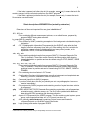
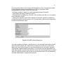
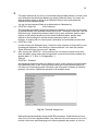
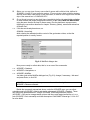
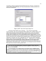
••fi Define a New project with
CRYSTAL > New Project.
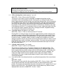
Define the Project Name and type in all known data (Fig. 2.1).
At least Crystal name, Crystal number, Working and Data directories must be defined. If
you leave Data directory blank, it will default to the Working directory. Do not worry too
much, the remaining items can be filled in later with CRYSTAL > Edit Project. As stated
previously, the combination of Crystal name and Crystal number must be unique. If it is
not, SMART will increment the crystal number. We strongly recommend that you use a
new directory for each crystal. Otherwise, old data can be easily overwritten.
Press Enter or click OK when you enter data and choose Small Molecule from the next
menu.
Fig. 2.1. ‘Crystal > New Project’ and ‘Crystal > Edit Project’ dialogue box.
Note: It is also possible to use the present configuration and to enter your temporary data
by the above-mentioned CRYSTAL > Edit Project command. However, we do not
recommend it, because in that case it will be easy to forget to define New Project later, or
some instrumental corrections could be out of date. A project can also be defined using
CRYSTAL > Copy Project and CRYSTAL > Config To Project commands. Once defined,
the project can be activated using CRYSTAL > Switch To Project.
•fi Center crystal optically with
!!!
GONIOM > Optical
(Ctrl+O shortcut)
or
CRYSTAL > Evaluate.
The latter command automatically performs optical alignment and takes a rotation picture.
For some slightly obscure reason, which we experts wish to keep to ourselves (but see
Preliminary notes), it is better to use the first option.
Do not forget to note crystal dimensions (maximum, intermediate and minimum) during
the optical alignment operation.
In any case a dialogue box appears with some pre-defined diffractometer angles. First of
all, check that they correspond to the goniometer used. (From time to time and for
7
!!!
unknown reasons SMART forgets the pre-defined base angles.4) For our P4 goniometer
they should be 2-theta = 0°, omega = 0°, phi = 60° and chi = –30° (or 330°). Then press
ENTER and find the manual box on a sidewall of the diffractometer cage.
When using the GONIOM > Optical command with default angles (marked A, B, C, and D
on the manual box)5 one of the slides on the goniometer head is always perpendicular to
the viewing direction. The 180° rotation around phi when activating the AXIS PRINT button
while keeping the same angular button depressed, is designed to adjust this slide, so that
the crystal is well centered after repeated 180° rotations. Positions A+B and C+D are
rotated to each other by 180° around chi (the first two hold the goniometer head pointing
up, the latter two pointing down).
For crystal centering we recommend the following procedure: Start with the A
button depressed and activate the AXES PRINT button to drive the goniometer to the
starting position. Adjust the crystal both in the horizontal and the vertical directions (note
the appropriate drivers on the goniometer head). Then depress B followed by AXES
PRINT. After this the crystal should be clearly visible (it is now in focus) so you can
adjust it precisely in the horizontal direction. The extreme left and right points of the
crystal should be equidistant from the center of the microscope cross (keep the
graduated scale horizontal, it can be rotated by gently turning the microscope eyepiece –
do not push the microscope sideways!). By repeating AXIS PRINT check the center point.
If it exactly coincides with the vertical line of the crosshair, the crystals outermost points
should be equidistant from the center after the 180° rotation. If the crystal is now shifted
to one side, adjust it in the opposite direction for half of the displacement, and note the
position of the center of rotation. Repeat AXIS PRINT with B depressed until the crystal
stays on the axis. Now depress A and do the final centering in this position (by repeated
rotations). Set the graduated scale (reticle) in the eyepiece vertical and finely adjust the
vertical position of the crystal. Now depress C or D and activate AXIS PRINT. While the
crystal rotates to the new position you can check it through the microscope (it rotates
almost through all possible positions).
It can well happen that SMART will choose to rotate around chi so that the goniometer
head runs into the beam-stop mounted on the collimator (according to Murphy’s law it
almost certainly will; see also footnote 4), although it could as well go the other way and
avoid it. Do not loose YOUR head and with it your crystal, collimator, or centering of the
microscope by making some stupid panic move. Just gently push the beam-stop around,
ahead of the racing goniometer head. It is easily moved, and the goniometer head could
do it by itself without any damage, but we suggest you do it with a gentle touch of the
human hand (here robots still cannot cope).
Readjust the vertical position if necessary by switching between A (or B) and C (or D),
and that’s it!
•fi If you prefer, it is possible to center the crystal without default positions. In that case use
GONIOM > Manual
(Ctrl+M shortcut).
Then press the desired axis button on the manual box and use the right-hand buttons
(fast, slow, forward, or reverse) to get suitable angle positions. Be careful, think about
collision danger!
Tip: It is easier to measure a crystal in Manual than in Optical mode. It might be better to wait
with the precise determination of crystal dimensions until you believe the crystal is
satisfactory (i.e. after the MATRIX operation).
4
5
SMART is not as smart as one could expect.
The left-hand buttons on the manual control box are usually labelled with both letters and angles.
8
!!!
After the crystal has been centered, lock the goniometer head slides and recheck the
crystal centering. Then press Esc to quit the operation. Close the doors, adjust until all
lights are green, and press the ‘Reset’ button.
•fi Again set the diffractometer angles to zero (GONIOM > Zero or F10 shortcut). Confirm
‘Yes.’
•fi If necessary, raise voltage and current to the desired values by
GONIOM > Generator.
!!!
Adjust the voltage first! Both parameters have to be increased in steps of 5 until the
normal values for our system, 40 kV and 35 (or 37) mA, have been reached (Mo tube).
•fi Perform
!!!
GONIOM > Home Axis,
which checks the calibrated position controls of the goniometer circles, so that the
reported positions are exactly consistent.
This command should be repeated four times, to home all four axes on the P4
goniometer (however, since default values are listed sequentially, it is enough to press
Enter to advance to the next axis).
Fig. 2.2. ‘Acquire > Rotation’ dialogue box.
!!!
Look at the pointers on the goniometer scales. They can easily get 1° away from zero
and Home Axis will not notice. If the pointers do not show 0°, use Manual mode and
position the goniometer circles close to zero. Then repeat
GONIOM > Home Axis.
•fi Take a rotation photograph (rotation around phi) by
ACQUIRE > Rotation.
Set the time if necessary (Fig. 2.2), but the shortest time is 72 seconds, and this value is
a good choice if the crystal is not very small. (There is a conflict in the manual here, see
pages 2-13, and it is not quite clear what is the shortest time allowed by the goniometer
rotation speed.) Leave default values for the other parameters. Beware, rotation
photographs are not stored automatically, but must be saved using FILE > Save if you
wish to keep them for documentation (a common extension for rotation photographs is
.rot).
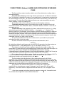
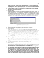
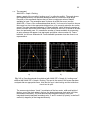
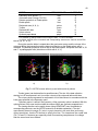
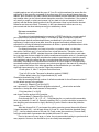
Some characteristic rotation photographs are shown in Fig. 2.3. The intensities of spots
can give you an idea about the measurement time required for a frame; the number of
spots gives you an idea about how many frames to collect for the initial lattice
determination. (If you think you do not see anything in your rotation photograph, try
another one with an exposure that is at least twice as long.)
9
a)
b)
c)
d)
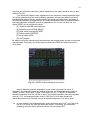
Fig. 2.3. Examples of rotation photographs: a) a poly- and micro-crystalline sample,
b) a polycrystalline sample containing several big and several small crystals, c) a good, single
crystal sample, d) the same as c), but with photo converted to a film-like view. (Note that the
last picture is not produced in SMART, but by screen capture and further handling.)
After making a preliminary choice, also make a preliminary scan of 10 frames. Continue
as follows:
Open the ACQUIRE > Edit MultiRun menu and edit to get only one line:
1 001 0 0 0 0 3 0.3 10 t
(t should be your estimated exposure time per frame in seconds).
After that, start ACQUIRE > MultiRun, give the name “Trial”, ”Test” or something like that
(this would be the name of the frames) and press Enter. When the operation is finished,
check the collected frames for appropriate exposure time. Maybe you are not quite
satisfied with the intensity of the spots and wish to increase the exposure time, or
perhaps the spots are so intense and nice that you can use a shorter time. But do not go
below 10 seconds per frame.
If the spots tend to appear on only one, or at most two sequential frames, you have to
decrease the step size called ‘Frame width’ in SMART. Increasing the step size to more
than 0.3° is not advisable, even if some spots continue through many frames. After
choosing the step size, make the following calculation:
N = 160 / [(number of spots) x (selected step size)].
This gives you an estimate of the number of frames, N, needed for a good MATRIX
operation (see later). However, values lower than 20 or higher than 60 frames are not
recommended.
10
Also, check the crystal quality with the ANALYZE > Graph and
ANALYZE > Graph > Rocking commands described in the next chapter. They can reveal
splitting of spots due to a fragmented or composite sample.
Tip: Your crystal is poor and yielded only a powder diffraction pattern (as in Fig. 2.3.a). Do
not give up immediately. Use a vector cursor described in the next chapter to measure
the diameter of at least three of the most prominent circles, read d-values (in Ångström)
to the right of the image and divide them by two. If any powder diffraction database is on
hand, use these d-values to search through the base. Who knows, maybe the structure
has already been described, or unit cell parameters have been determined before, or you
have another example of isostructural compounds and isomorphous replacement, or …
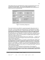
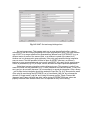
Fig. 2.4. ‘EDIT > Config(uration)’ dialogue box.
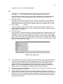
••fi If the crystal is not discarded after the previous operation, the next step is acquisition of
an orientation matrix. Before that, invoke
EDIT > Config
and check the diffractometer configuration (Fig. 2.4). Input proper ‘Source kilovolts’ and
‘Source milliamps’ values. Check with your system administrator that you have the correct
‘Sample-detector distance’ and the correct ‘Direct beam X’ and ‘Direct beam Y’ center.
Check also if the proper FloodFld (flood-field correction) and Spatial corrections are used.
For our detector, at the bottom right in the SMART window both fields should contain the
same code, h423l17 (extensions are not visible). Be sure to have a Dark-field correction
of appropriate time (the same as you use for the exposures in Matrix). See description of
._dk files in the beginning of this Guide. If necessary, load one from the c:\frames\ccd_1k
(FILE > Load Dark), which has the most recent date.
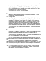
•fi After that invoke
ACQUIRE > Matrix, or the equivalent CRYSTAL > Unit cell.
These commands automatically collect three (short) series of scans at different starting
angles, clear Reflection Array, invoke Threshold and store some collected spots into the
Array, perform Autoindexing procedures, perform least-squares on the reduced primitive
cell, determine the Bravais lattice, perform a least-squares refinement of the resulting unit
cell, and finally write the new cell parameters into a .p4p file.
11
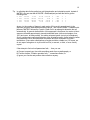
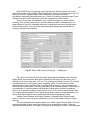
Choosing proper values in the corresponding dialogue box (Fig. 2.5) should be possible
by the checking procedure described above, but be sure that some skilled
crystallographer is on hand. In short, the values are:
- ‘# Frames’ (number of frames) in a series preferably between 20 and 60,
- ‘Frame Width’ preferably between 0.2 and 0.3°,
- ‘Seconds/frame’ preferably from 10 to 60 s, but it could be even 180 s, for very small or
poorly diffracting crystals.
- ‘Indexing HKL tolerance’ and ‘LS RLV tolerance’ should be 0.1 and 0.01, respectively,
for expected excellent quality crystals, or 0.2 (no more than 0.25) and 0.02, respectively,
for expected problematic cases.
Fig 2.5. ACQUIRE > Matrix dialogue box.
If you did not change ‘Job name’ (why should you?), the collected frames will be named
from matrix0.001 (matrix1.001, matrix2.001) to matrix0.xxx (matrix1.xxx, matrix2.xxx),
where xxx is the number of frames in each series defined by the ‘# Frames’ argument.
If the MATRIX operation finishes successfully, you will obtain initial cell parameters and
other data required to perform data collection. In that case, the working directory contains
smart.ini, three sets of matrix data, as well as the orientation matrix, unit cell parameters
and other data needed in a proper matrix#.p4p file.
12
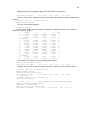
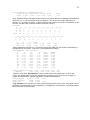
Tip: In collecting data for the preliminary cell determination and orientation matrix, instead of
MATRIX you can start with ACQUIRE > EditQuad(rant) and edit the field to get the
following lines:
0
1
2
3
001
001
001
001
-28.00
-28.00
-28.00
28.00
-5.00
-28.00
-28.00
28.00
70.00 -110.00
104.50
4.00
-20.50
26.50
9.50 -16.50
2
2
2
2
.300
.300
.300
-.300
n
n
n
n
t
t
t
t
where n is the number of frames in each series (40 is usually enough) and t is the
exposure per frame estimated as described above. Then use ACQUIRE > Quadrant with
jobname “MATRIX” followed by Crystal > Redtn Cell in an attempt to determine the cell
automatically. A general characteristic of this approach is that these four series of short
scans are directed approximately toward tetrahedral faces (with mutual angles of ca.
109°) and cover, at least partially, the whole reciprocal space (not only a hemisphere).
So you could expect easier determination of the orientation matrix, faster indexing, better
cell parameters, much less parameter correlation and even refinement of crystal
translations. (Some other combinations of angles could be suitable too.) Of course, we
do not expect a beginner to try this with her first (or second, or third, or even fourth)
crystal.
If the attempt to find unit cell parameters fails, ... then you can:
a) Choose to spend your time with something easier than crystallography, or
b) Find the chapter “If Matrix operation fails ...” somewhere below, or
c) Ignore your results and perform data collection anyway.
13
Three-circle platform diffractometer
If you are using a platform diffractometer with fixed chi and a video camera, this section
is for you!
Be aware, however, that only operations specific for this type of diffractometer are
described here. Therefore, your idea to skip the first part of this chapter was totally wrong.
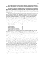
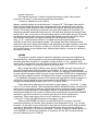
Most SMART diffractometers are built with the phi mechanism set at a fixed chi, mounted
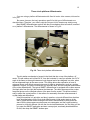
on a “platform” diffractometer. The diffractometer is shown in Fig 2.6.
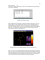
Fig. 2.6. Three-circle platform diffractometer.
The phi rotation mechanism is housed in the block that sits on top of the platform, off
center. The phi rotation axis is tilted 54.74° from the horizontal. In case you wonder, the 54.74°
angle is the same as the angle between a body diagonal and a face diagonal in a cube, when
the two diagonals begin at the same corner. This design allows the exploration of most of
reciprocal space, and affords convenient access for add-on attachments, such as a cooling
apparatus. In short, you get the functionality you normally need, but with a simpler machine than
a four-circle diffractometer. The typical SMART diffractometer is equipped with a video camera
(the black tube from the right) that replaces the telescope. The video camera provides a clear,
magnified picture on the computer screen of the area near the crystal. This picture makes it
easy to adjust the crystal position. It also allows for reasonably accurate measurements of
crystal shape and dimensions.
Using this machine is in principle, and also in practice, not much different from what has
been described above for the four-circle diffractometer. Initial project start-up is the
same, crystal selection and mounting are the same, data collection is pretty much the
same. But the video camera requires some new commands, and the crystal centering
process is a little bit different. As with the four-circle diffractometer, the first thing you do
is to open the SMART application and start a new project, as already described above.
Do this; then keep the SMART window open.
14
Fig. 2.7. Top of Video window with explanation.
When you have finished setting up SMART, you will start the video camera. On your
desktop there is a binocular-shaped icon named Video. Double click this icon. The camera
window opens. At the top of the window is a menu bar. Below that there normally is a
toolbar. If the toolbar does not appear, open the View menu and select Toolbar. Fig. 2.7
shows the top of the video window with the toolbar open. The functions of the most
commonly used buttons are also indicated in the figure.
To start the video running, click the button with an icon that looks like a dog-eared page to
open a new image, then click the button with the black and green arrow-shaped icon to
start capture.
Fig. 2.8. The Video Tools > Options dialogue box.
You can select the shape of the grid that appears on the screen. Most people like the
circular grid (see Fig. 2.10 below), but you are of course free to select any grid you
want. The grid is often referred to as a reticle. You can also set the orientation of the
grid. To do this, select
•fi TOOLS > Options menu.
In the box that appears (Fig. 2.8) you can type in the tilt in degrees. The fixed chi angle is
54.7°, so if you set the reticle tilt to 35.3°, the grid x-axis will be parallel to the phi rotation
axis when phi is perpendicular to the optical axis of the video camera. This tilted grid
orientation makes centering more intuitive for most users. When done, click OK.
At this stage it is a good idea to verify that the center of the reticle on the video screen
corresponds to the diffractometer center. For this you can mount a pin with a sharp tip in
the crystal position. In our laboratory we use the tip of a fine sewing needle attached to a
15
regular mounting pin, but any pin with a well-defined tip will do, including most mounted
crystals. Detailed, step-by-step instructions follow. This procedure should be done quite
frequently, but not necessarily for every crystal.
1.
Orient the phi box so that it is in a good position for crystal mounting. For this you make
the SMART window active and select
•fi Goniom > Optical.
In the window shown in Fig. 2.9 define starting values for two theta, omega and phi. The
values we use are –30, 150, 0, respectively. These angles will position the phi axis in a
plane perpendicular to the camera optical axis. Click OK. On the manual control box push
D and then the AXES PRINT button. This will bring the angles to the values in the ‘Optical’
window (if it does not, get the person responsible for the diffractometer to help you).
Fig. 2.9. The ‘Optical’ dialogue box.
2.
Determine the actual x-axis. Make the video window active and select
•fi Tools > Options.
Check if the reticle tilt is 35.3° (Fig. 2.8), if not type in this value. Make sure the video
capture is active. Mount the pin with the tip attached. Adjust the goniometer head so the
image of the tip just touches the y-axis (y points more or less in an up direction) of the
reticle. Then use the perpendicular slides of the goniometer head to center the tip so it
appears stationary when phi rotates (it is not yet necessarily on the reticle x-axis).
You control phi rotation from the manual control box. Pressing AXES PRINT alone causes
phi to rotate 180°. To rotate phi 90° depress the currently undepressed button C or D and
press AXES PRINT.
!!!
Make sure the tip of the needle remains stationary during a 180° phi rotation when you
are done with this step.
The needle tip is now positioned on the actual x-axis. It may or may not coincide with the
reticle x-axis. If the actual and reticle x-axes coincide (the needle tip is at the origin) skip
to step 4.
3.
If needed, position the reticle x axis correctly. Go (in Video) to the
•fi Tools > Options
4.
dialogue box, click the ‘Select Origin’ button, then OK. Carefully position the mouse pointer
at the tip of the needle, then click. Be careful not to click prematurely. The x-axis should
now be correctly set, and the needle tip should be at the current origin.
Next you will determine the position of the y-axis, and with that the true origin. To do this
you rotate omega 180° by pressing A and then Axis Print. After the omega rotation, note
the position of the tip on the screen. If it is still at the origin, then everything is fine, and
you are done. If it is not, find the midpoint between the current tip position and the current
origin. Then move in a vertical direction on the screen (in your mind) until you reach the xaxis. This point should be the correct origin. From the Tools menu select Options. Click the
Select Origin button, then OK. Position the cursor at the determined origin and click the left
mouse button. Be careful not to click prematurely.
16
5.
Repeat the whole procedure to double check that the origin has been properly set. When
done, return omega and phi to the default start positions by pressing D, then Axis Print on
the manual box. Remove the calibration pin from the goniometer head and store it in its
proper place.
Now is the time to mount your crystal. Select the best crystal you can find and attach it to
the mounting fiber. Position the mounting pin in the goniometer head. Make sure the video
window is active. An example is shown in Fig. 2.10.
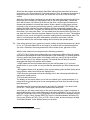
Fig. 2.10. Screen image of a crystal. The crystal is not yet quite centered.
Center the crystal on the phi axis, and adjust the height. The procedure is similar to that
described above in steps 1 and 2. Because you know the true origin of the reticle, it is
not necessary to rotate omega. When you are done, the center of gravity of the crystal
should remain at the origin at any phi value.
At this time you should measure the crystal dimensions. Click in the SMART window and
select manual mode
•fi GONIOM > Manual,
then click OK. Click in the Video window. Select the vector cursor (see Fig. 2.7).
Because the diffractometer is in manual mode you can adjust phi, and perhaps omega
with the manual box, for best viewing.
You measure a desired length by clicking at the starting point, then move the cursor to the
end point. Below the lower right area of the picture is a window that shows some
geometric parameters; among them is the length you want. Write it down, and continue
measuring until all desired dimensions are done.
At this stage you should quit Video. On some systems there seems to be interference
between Video and the SMART display.
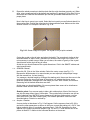
Rotation photo. You are now ready to take a phi rotation photo. Most of the time you
can skip this step without loss of information. The crystal quality information can just as
well be obtained from ‘MATRIX’ frames (however, by taking a rotation photo, you can
save some time in the case of bad crystal). The Rotation procedure is similar to that
described above. Rotation is reached by
•fi Acquire > Rotation.
A menu similar to that shown in Fig. 2.2 will appear. Set the exposure time to 60-180 s,
and set the other parameters as shown in the figure, except that making chi = 54.74° has
higher aesthetic value (it is probably preset anyway). Click OK. See above for other
aspects of the rotation photo and compare Figs. 2.3 and 2.11. Note that the axis of the
picture is tilted 35.3° relative to the horizontal direction on the screen.
17
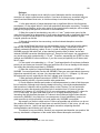
Fig. 2.11. Examples of rotation photographs obtained on three-circle platform diffractometer:
a) low-quality crystal (picture supplied by Dr. Marilyn Olmstead), b) good-quality crystal (note
the weak odd layers).
Unit cell determination. Initial determination of the unit cell is essentially the same as
explained above, so it will not be discussed here. The commands are:
•fi ACQUIRE > Matrix > OK > Options.
A typical value for the number of frames entered under Options is 20. If the crystal is
very small, or it diffracts weakly, a larger number (36-40) can be used. Be sure to save
the results as described for the four-circle diffractometer.
18
Notes on low-temperature data collection
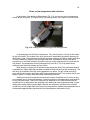
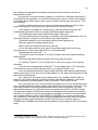
In the picture of the platform diffractometer (Fig. 2.6) you can see the low-temperature
nozzle above the crystal. The figure below is a close-up photo of the region near the crystal.
Fig. 2.12. Arrangement of mounting pin and cooling nozzle.
In the background is the face of the detector. Top, pointing down, is the tip of the nozzle
for the cold stream. The outside of the tip is held at room temperature by electric warming. No
shield gas is used. The goniometer head holds a copper mounting pin with an empty glass fiber.
The pin is made from copper to allow enough heat to be transferred to the tip of the pin to
prevent frost. In the lower middle of the picture one can see a small amount of fog around the
cold stream. The temperature at the crystal position is near 90 K. The X-ray beam tunnel
(collimator) and the beam catcher are also visible.
Note the way the copper pin is attached to the goniometer head. The goniometer head is
a standard xyz Supper head that has been modified to allow side entry of the mounting pin. The
side entry is necessary when the cooling apparatus is in place. The pin is held securely in
place with the little screw containing a small, spring-loaded steel ball. For mounting, the pin just
snaps in place; it is easily removed without loosening any screws.
With this set-up both crystal and crystal mount remain completely free of ice for as long
as is needed, also in very humid weather. Crystal mounting for low-temperature work tends to
be very fast and simple. There is no waiting for an adhesive to set. Data collected with the
crystal near liq. N2 temperature are generally much better than room-temperature data. Crystal
decay and crystal movement during data collection are eliminated. Intensities from a cooled
crystal can be much higher than from one at room temperature; displacement parameters are to
a reasonable approximation proportional to the thermodynamic temperature (in K).
19
3. HOW TO ANALYZE CRYSTAL DATA
No matter how successful you were during unit cell determination and data collection
procedures, it is a good idea to examine the crystal data in more detail. This can be done by
careful inspection of the corresponding frames with the help of the following commands that
belong mainly to the ANALYZE menu.
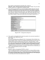
••fi First of all, choose the desired frame to be displayed on the screen with
FILE > Display, ANALYZE > Display, or, simply, Ctrl+D.
Sometimes, as shown in Fig. 3.1, it is necessary to enter the full path together with a
frame name. Actually, if you choose any frame from a set of data, the whole set
becomes available for analysis. For example, if the current frame is name1.009, all
frames from name1.001 to name1.xxx, where xxx is the number of frames in set 1, can
be analyzed. Leave the other parameters in the dialog box as they are.
Images of the next or preceding frames can be obtained by pressing Ctrl+Æ and
Ctrl+¨, respectively.
Tip: When one frame in a series is displayed, Alt+Æ and Alt+¨ runs rapidly, like a movie,
through the series – a really nice review of collected data.
Fig. 3.1. ‘FILE > Display’ dialogue box.
If the lattice has already been determined you can check the small ‘Add HKL Overlay’ box
in the ‘File > Display’ menu dialogue box. An overlay of predicted spot positions that uses
the current (see below) orientation matrix from a .p4p file will be drawn on top of the
frame every time a new frame is displayed. Note: A box displayed on the screen means
that the reflection center, RC, is in the scan range of the current frame, a circle means
that RC is in the preceding frame, a cross means that RC is in the following frame.
It is sometimes helpful to compare two or more (up to four) frames on the screen. Go
back to the ‘FILE > Display’ dialogue box (Fig. 3.1) and pay attention to the 'Quadrant'
window. Default value ('0 Full') means that only one frame will be displayed at the time
using full screen. With 'Quadrant' window opened it is possible to display half-sized
frames in one of the quadrants (low left, low right, etc.)
•fi If you are not sure about the current orientation matrix, use
20
FILE > Read .p4p
in order to check or replace the orientation matrix.
A command that is very similar to the FILE > Display is:
•fi ANALYZE > Display > HKLs,
at first sight not a very useful command, since this time an overlay will be drawn only
over the currently displayed frame. You can use this command to adjust ‘Spread’, i.e.
width (in degrees) of the predicted frame, but the default value (0.75°) is a good choice.
However, on occasion, if the spots are very weak or very intense, it is difficult to
analyze displayed frames. In this case it could be helpful to use the previous command
for increasing/decreasing the thickness (‘Lineweight’) of the overlay lines. A value of 1.5
or 2 really helps!
At the same time, you can try to adjust screen contrast and brightness using
•fi EDIT > Contrast (or Ctrl+T shortcut).
Dragging the mouse left or right with the left mouse button depressed changes the
contrast. Drag to the left to increase the contrast and to the right to reduce it. This is
analogous to a contrast control achieved by changing aperture or sensitivity of a
photographic film. Dragging the mouse up and down changes brightness, analogous to
different exposure times of a photo. Notice changes in the color scale on the right side of
the SMART screen! Note: It is possible to use the arrow keys or a combination of arrow
keys and the Ctrl button for the same purposes. Release the left mouse button to exit and
save changes, press Esc or the right mouse button to exit and reset color mapping to the
default level.
•fi Very similar to the FILE > Display command is
ANALYZE > Load,
but there you can optionally make and display a linear combination of two frames.
•fi Header of the current frame can be viewed using
ANALYZE > Frame Info.
•fi Any square area on the display can be zoomed using
ANALYZE > Zoom,
when a crosshair cursor appears. Once the center of the area to be zoomed has been
selected, press Enter or release the left mouse button in order to see a pop-up menu,
from which you can choose the magnification factor: 1, 2, 4, 8 and 16x (or Exit). Press
the right mouse button to escape from the zoom menu.
•fi A Crosshair cursor is obtained by invoking
ANALYZE > Cursor, or by pressing the F5 shortcut.
At the same time several useful quantities (coordinates of crosshair center, counts at
current pixel, 2-theta value at current pixel, resolution (in Å) of current pixel, hkl values if
orientation matrix is in effect, etc.) are displayed to the right of the image. Press the left
mouse button, or Enter key to finish.
21
Valid for all kinds of cursor:
Pressing Ctrl can speed up cursor movement.
It is possible to drag the cursor with the arrow keys. This is much more precise!
•fi A Box (rectangular) cursor appears if you call
ANALYZE > Cursor > Box or press F6 shortcut.
This cursor is very useful if you are interested in integrated intensities and the
coordinates of the corresponding centroid. Pressing Esc or clicking the right mouse
button toggles between position-change mode and size-change mode, so you can adjust
box dimensions. Move the box to the approximate position, press the right mouse button
and tune the box dimensions, then press the right mouse button again and position the
box properly. Finally, press the left mouse button or the Enter key. As above, to the right
of the image you will see: X,Y coordinates of the box center, height and width of the box,
sum of the pixel values, maximum pixel value, average pixel value, integrated intensity,
X,Y coordinate of the centroid of intensity, etc.
•fi A Circular cursor will appear if you invoke
ANALYZE > Cursor > Circle or use the equivalent F7 shortcut.
Pressing ESC or clicking the right mouse button toggles between position-change mode
and radius-change mode and allows adjustment of the circle radius (see above). Press
the left mouse button or Enter key when finished. The right-side output is similar to that
for the box cursor. In addition, radius of circle in 2-theta and in Ångström, as well as
changes required to the phi axis position and to the goniometer head arc in order to move
the diffracted layer circle to the beam center are shown. (If you are using a goniometer
head with arcs this will help you to orient a desired and marked zero-layer to coincide
with the primary beam.)
•fi A Vector cursor appears if you invoke
ANALYZE > Cursor > Vector or its F8 shortcut.
The primary use of this cursor is to measure distances on the displayed frame. The
cursor is of the rubber-band type. As before, pressing Esc or clicking the right mouse
button toggles between position-change mode and size-change mode. In the latter case
the vector origin stays fixed while its end point moves as the mouse is dragged. The
output to the right contains counts of pixels at vector origin and endpoint, X and Y
coordinates of the origin, endpoint and midpoint, length of vector in pixels, degrees
2-theta and Ångström.
•fi If you wish to see a one-dimensional slice (or profile) through pixels of the current frame
use
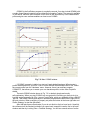
ANALYZE > Graph.
This command is very much like the preceding, ANALYZE > Cursor > Vector. Vector start
and end points are fixed in the same manner. When you have specified the cursor
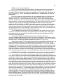
position, the program plots intensities along the cursor path in an X-Y graph (Fig. 3.2.a) of
intensity versus vector line. The right-side output contains details very similar to those
displayed after execution of ANALYZE > Cursor > Vector.
22
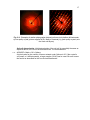
•fi The command
ANALYZE > Graph > Rocking
draws a graph of the so-called “rocking curve” (or reflection profile). The graph shows
the integrated intensity of a specified rectangular area as a function of scan angle.
Execution of this command requires that you have a contiguous series of frames
available for input. The rectangular area is chosen by a Box-like cursor (see the
ANALYZE > Cursor > Box command described above). You have to be careful to choose
the correct box size in the appropriate dialogue box, or to correctly resize the box on the
screen! The other important parameter is ‘Frame halfwidth’, which defines the number of
frames on either side of the current frame to be included in the curve. It should be at least
three, but preferably more. If it exceeds the number of frames available for processing,
an error message will appear. Just start again and define a lower number for ‘Frame
halfwidth’, but a curve obtained with ‘Frame halfwidth’ parameter less than three is not
representative.
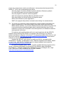
a)
b)
Fig. 3.2. (a) One-dimensional slice obtained with ANALYZE > Graph; (b) “rocking curve”
obtained with ANALYZE > Graph > Rocking. The spot in the center of the screen has been
analyzed after an appropriate zoom. Note that the spot is bad looking and that reflections
should not be split.
The screen output shows: X and Y coordinates of the box center, width and height of
the box, sum of the pixel values in the box, the largest and mean pixel value in the box,
the standard uncertainty, 3D (three-dimensional) integrated intensity of the spot,
integrated intensity/standard uncertainty ratio, X- and Y-centroid (in pixels), as well as Zcentroid (in degrees) of the integrated intensity.
23
4. RECIPROCAL LATTICE DISPLAY PROGRAM
A very powerful program for data checking is Reciprocal Lattice Display Program
(RLATT). It displays measured data in reciprocal space. Various reflection files can be used for
input: .p4p (from SMART, indexing not necessary), .raw (from SAINT), .hkl (from SHELXTL) and
some less important files (for the complete list see RLATT manual). In order to have the proper
orientation matrix, before a .raw or .hkl file you must read a parameter (.p4p) file. Use
‘Reflections’ menu to choose the file, to add reflections (more than one reflection file can be
displayed at the same time), or to remove (‘Clear’) reflections.
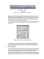
Once you have loaded a file, the brightness of screen spots corresponds to the
reflection intensities; it can be adjusted with the slide bar on the right side of the screen. While
reflections from .raw or .hkl file are always cyan, reflection from a .p4p file are coded
according to the ACSH flags (flags are described in the next chapter):
white - reflections with all flags,
magenta - missing C and H flag,
yellow - missing A flag,
red - missing C flag,
green - missing H flag,
blue - missing S flag.
This list is also available from the Help > Quick Color Reference menu (but read the RLATT
manual for the order of priority). A lot of colored spots usually implies an incorrect cell or a
composite crystal.
Reflections shown on the screen could be toggled or filtered. Toggling reflections on and
off is simple, just press the first letter of their color. Filtering (‘Filter’ menu) is a little more
complicated, but offers more options – reflections could be filtered by any combination of flags,
indices and resolution parameters.
If you do not like the blue (default) background color, change it from the
Display > Background Color menu. It is, however, more important that from the Display menu
you can choose to show direct space, reciprocal space or laboratory axes.
The projection can be rotated in real time by dragging the mouse with the left button
depressed or with the cursor keys. Just open the ‘Display’ menu and check ‘Rotate’ mode.
The mouse commands are:
Left button + drag – rotate the lattice,
Middle button + drag backward or forward – zoom in or zoom out,
(Ctrl + Alt keys + left button emulates the middle mouse button)
Right button + drag – pan the lattice,
(Ctrl key + left button emulates the right mouse button)
The keyboard commands are:
The arrow (cursor) keys rotate the lattice around the X (↑,Ø) and Y (¨,Æ) axes. Rotation
around Z is done with the Insert and Delete keys. Note that X is horizontal on the screen, Y is
vertical on the screen and Z perpendicular to the screen.
Gray + and – signs means zoom in and zoom out, respectively.
Press the Shift key to speed up rotation, or the / key to slow down rotation.
Available shortcut keys are:
F1 – rotate 90° about X (horizontal on the screen),
F2 – rotate 90° about Y (vertical on the screen),
F3 – rotate 90° about Z (coming out of the screen),
Shift + F5-F8 – save the current orientation,
24
F5-F8 – restore a saved orientation.
RLATT is extremely useful and you should run the program as often as necessary to
check the regularity of the reciprocal lattice and the values of the unit cell parameters. If
everything is OK, you should see regular rows parallel to the reciprocal axes. The phrase “as
often as necessary” means: each time you determine, or re-determine the unit cell
parameters.
First of all, in case you see curved rows, or even duplicated spots, do not blame your
crystal or your whiskey; most often it turns out to be an artifact of inaccurate detector
correction values (X, Y for the detector center too far off, or more often a wrong detector
distance), so check and try to correct this. If you sometimes see a nice circular orbit of spots in
close succession, it is an almost unmistakable sign of "hot spots" being included in your list of
reflections. If you are the type that likes to read telephone books or such, just go to your
reflection list (Edit > ReflArray in SMART) and look for repeating, almost identical Xs and Ys.
Delete them (maybe back up your list first) and check again. Bet your orbits have disappeared.
Another easier approach is to mark graphically the “ghost” spots in RLATT (see later how to
change flags and colors of the reflections), save the results in a file, edit it by throwing out the
marked reflections and then use the edited file in further work.
It is not obligatory to have the true unit cell parameters in the .p4p file you use. It is still
possible to verify the lattice regularity and measure distances between layers. Although the
measurements are not very accurate, the obtained values are good estimates for the next
round of unit cell determination.
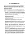
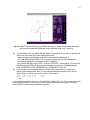
How to measure distances between layers? Turn on Measurement mode
(Display > Measure distance) first and zoom in the picture if necessary. Then drag the mouse
with the left button depressed between the chosen start and end points. After you release the
left button RLATT will show the distance between two points in Å-1 (Fig. 4.1.a).
In this version of RLATT (3.0) there are two very good tools that help measurements. Use
them to increase the accuracy of your determination! If you press the Gray + key, you will
subdivide the current measurement with the new distance shown. It is, of course, possible to
repeat this operation many times. In the opposite direction, the Gray – key reduces the number
of subdivisions. If you press the Page Up key, you will add extra divisions on each side of the
existing one (Fig. 4.1.b). They are of the same length as the previous divisions. (The Page
Down key reduces the number of extra divisions.) For fine tuning you can use the cursor keys,
which move the measurement tool, or Insert and Delete keys, which rotate the lattice around Z.
With RLATT it is also possible to see if the lattice is rectangular or not and to estimate the
angles. The program is also useful for testing lattice centering. Try the following approach:
Turn the lattice until you notice a family of lattice planes with the largest spacing and
orient it for an edge-on view. Measure the interplanar distance (the length of the corresponding
crystal lattice vector, call it a). Now turn the lattice parallel to the planes until another family of
planes with a relatively large spacing appears. Try now to adjust the picture so that the new
family of planes is oriented horizontal or vertical and you still see both families edge-on (not an
easy task!). Measure the second interplanar spacing/crystal lattice vector (call it b). If you have
some applicable angle-measuring device you can try to measure the angle between the two
plane families/vectors (gamma) on the screen. Now turn parallel to the second family of planes
with the help of the cursor keys (one click turns exactly one degree!) or with F1 or F2 (a 90degrees rotation) until you see another good family of planes edge-on. Counting the clicks with
the cursor keys measures b*. The interplanar spacing of the third family gives the c-parameter,
angle-measuring on the screen gives a. Positioning the third family of planes vertical or
horizontal and then turning by cursor keys until the first family of planes reappears edge-on
gives a measure of g*. a*can now be measured by rotating the first family of planes until the
second reappears again. If this was a triclinic case, let’s hope you remembered to keep your
axes oriented properly right-handed, and know how to use the elementary lattice mathematics
to calculate the final values!
25
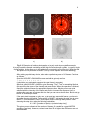
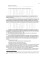
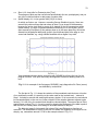
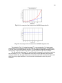
Fig 4.1. Examples of the RLATT
screen output.
(a) A triclinic reciprocal lattice
with measured distance between
two layers.
(b) The same lattice with added
divisions showing that the
measurement is not so good.
Pay attention to the superstructure effects indicated by the
presence of weak reflections
between the main layers.
Therefore the true c axis is
doubled with respect to the value
shown.
Change of reflection flags (or colors, see above), is also possible if the graphical editing
mode is in effect. In the Edit menu you can choose to change (Edit > Delete or Add a flag) one
or more flags. When ‘Selection box editing’ is activated, with the left mouse button depressed
one can draw a box enclosing one or more RL points. Then press Enter to change flag(s) of
spot(s) inside the box; this should be followed by color changes, too.
It is assumed here that you are in trouble after the automatic MATRIX operation, since, as
mentioned above, SMART picked up too many “hot spots” and was not able to index your
reflections. Try to identify these spots and delete their A and/or S flags. Since reflections
present in the Reflection Array always have A and S flags, deleting just these flags will later
help you recognize and erase changed reflections. Finally, save your job using EDIT > Save
results to a .p4p file.
There is another option for graphical editing if ‘Lattice overlay editing’ is invoked from ‘Edit’
menu (see RLATT manual for description), but so far we have found no use for it.
26
Some limitations of the program have to be emphasized. It is not possible to read out the
angles or indices of individual lattice spots (although the latter can be guessed by counting in
3D). Also, it would be very desirable to define shortcut keys that will display projections along
either reciprocal or direct axes.
27
5. IF MATRIX OPERATION FAILS...
That happens more often than anybody wants and it is always very frustrating. The
question is: How to recognize the failure? The first case is very simple: if MATRIX was run in
automatic mode, any screen output after the procedure is missing. Apparently, SMART was
totally confused about your crystal and its reflections (and probably about you as well).
However, sometimes the procedure offers really “funny” solutions with unit cell parameters of,
say, 80, or even more Ångström. Finally, the results could be quite different from what you
expected (reconsider expectations).
It could be worth noting that some experienced crystallographers pay little attention to the
MATRIX procedure, which serves them chiefly to verify that the crystal is suitable for data
collection – even if perhaps twinned. However, even they must pass through determination of
unit cell parameters and orientation matrix after data collection and before starting the
integration. Therefore, the procedures described here are universal, and they wait for you
here, there or in both places.
As a beginner, you have to analyze frames and reciprocal lattices (as described above),
as well as reflections picked automatically or manually during the MATRIX operation. They
are stored in a Reflection Array, which contains reflections used (or to be used) for unit
cell determination. Running any of the following commands:
•fi EDIT > ReflArray,
CRYSTAL > Redtn Cell > Edit, or
Ctrl+E shortcut
!!!
will allow you to view and possibly edit the contents of the Reflection Array. An ACHS
flag indicates the status of reflections.
- A flag means that the reflection record includes goniometer setting angles and X, Y
coordinates of the reflection relative to the detector origin; this is always the case for
reflections determined experimentally.
- S flag indicates that the values of the X,Y spot positions of this reflection have been
corrected with a spatial correction; this condition is also always satisfied for
experimentally determined reflections.
- C flag denotes centered reflections, that is, there was enough information to determine
the centroid inside the scan angle; the necessary condition is that the reflection is visible
on (or spanned by) more than one frame.
- H flag means that the reflection has HKL indices; of course, this is possible only after
indexing.
The other data in Reflection Array are: HKL indices (if determined), 2-theta, omega, phi,
and chi angles, X and Y detector coordinates of the centroid, normalized intensity (I) and
I/sigma ratio.
It is possible to modify any entry, to change flags, to delete some, for example, very
weak or very strong reflections, to type in some already known data, or to add some
reflections by an interactive means provided by CRYSTAL > Redtn Cell > Pick, which will
be described below.
Be very careful, one of the SMART bugs flies around, watching and waiting for you to fall
in its trap. After you finish editing the Reflection Array it is normal to click OK to accept its
new contents. Everything will be OK. However, if you meanwhile get the idea (very
clever) to press Write in order to save data (as an ASCII name.txt file for example) on
disk just for reasons of insurance, possible future usage, or just for documentation, and
if something in Array is accidentally marked (blue background, white letters), only the
marked part of the Array will be written to disk. A really amusing extraterrestrial
phenomenon! It is, indeed, so easy to lose all of your several-hours effort, especially if
data in the current matrix#.p4p file were later “spontaneously” (as defined by Murphy’s
law) rewritten, reindexed, etc. The same is true for printing.
If the problem is wrong or missing indexing, there are at least six ways to proceed.
28
First of all, you can try to use and index/reindex (perhaps with some modifications)
reflections already present in the Reflection Array. Sometimes only a small push is required to
“help” the program find the “proper” solution(s). Here the Reciprocal Lattice Display Program
and procedures described in the previous chapter could be very helpful.
If there is a suspicion of a composite crystal (twin or another intergrowth) we strongly
suggest you try indexing by GEMINI as a second option.
The third and fourth options imply that you will collect (automatically or manually) a new
set of (medium to strong) reflections and attempt to index them.
The remaining two cases are in fact obvious, but we wish to leave them for the end of
the chapter. (Why discourage beginners immediately?)
If you have been following our suggestions, you have already checked the collected
reflections using RLATT and got an idea about their usability. If it all looks just like a mess, you
could probably try autoindexing as described under option no. 1 by changing some parameters
blindly. Maybe the program sees better than you and you really get something (but need to
check to see if it is reasonable anyway). If you fail a few times, we suggest you do not waste
your time anymore; proceed to the next options.
If you have seen the light (a real lattice!) then you are probably in a hurry to try approach
number 1 right away. Good luck, you impatient soul! Oh, you took your time and already
measured some lattice parameters? For your bureaucratic type there would be no problem to
enter the expected parameters and small tolerances in procedure no. 1 and check 'Assume
known cell' (see later).
Maybe you have seen too much light (several lattices in a beautiful confusion). Skip
immediately to option no. 2. Again you could be without any quantitative data, or with quite a
detailed premeasurement in RLATT, but it depends on how you do other things in your life and
you will be rewarded accordingly.
1.
If you decide to use collected reflections, i.e. reflections already present in the Reflection
Array (perhaps with some above-mentioned editing), check the number of reflections in
Array. Remember: a maximum of 999 reflections can be stored in Array, 25 is an absolute
minimum for indexing, and, in accordance with BRUKER recommendations, a number in
the range 50-100 is about optimal at this stage. All reflections should be centered, i.e.
have a C flag! Delete all non-centered reflections and all reflections with I/sigma less than
30, or even 50, if you have too many suspect reflections in the Array. An alternative
approach is to identify “hot spots” using RLATT, as described above, and to remove them
from the Array. After that you can go to
•fi CRYSTAL > Redtn Cell > Index or Ctrl+X
which is also called “Autoindexing”. This command uses reflections stored (by Threshold
or by manual picking) in the Reflection Array to determine indices, a rough crystal
orientation matrix and a reduced primitive cell. The autoindexing procedure is based on an
algorithm operating on difference vectors (which are classified in groups) derived from
the input reflections. If the procedure with difference vectors fails, the program tries
indexing on full vectors.
If you really believe that you know the true unit cell parameters (maybe they were
determined previously, e.g. with the program RLATT, or you think you know them by
some providence, or those from MATRIX were good and you are in trouble after data
collection), go to the ‘Autoindexing’ menu (Ctrl+X), input the expected values for cell
edges and angles, enter ‘Length tol’ 0.1, ‘Angle tol’ 0.1 and check the small box (Fig. 5.1)
near the ‘Assume known cell’. How the latter option influences the behavior of the
program it is very hard to guess, but anyway... only a few seconds will be enough to
reach extreme happiness or total devastation.
29
If the attempt with known cell parameters fails, change some parameters shown in Fig.
5.1 and run the program again ... Yes, it is much easier said than done. What
parameters? If you do not have any idea about the parameters and your guess did not
bring any result, then try playing blindly.
Fig. 5.1. ‘Autoindexing’ dialogue box.
First of all, the default values (80 Å) for expected axis lengths (‘Expected unit cell’: A
axis, B axis ...) are very stupid (well, sorry protein folks!). In combination with ‘Length
tol’(erance), with a default value of 0.75, they define a possible interval for axis lengths.
The limits are between EAL*(1-FCEL) and EAL*(1+FCEL), where EAL is expected axis
length and FCEL is axis length deviation (if ‘Length tol’ is equal to 1 or bigger, the lower
limit is defined as 0.01). Try with values of 20 or 25 Å for axes and 1 for ‘Length tol’, or
with the best-guessed values obtained, for example, during previous analysis of frames
(ANALYZE > Cursor > Vector, do you remember?). As already stated, ‘HKL tolerance’
should not be bigger than 0.25 or 0.3.
At this stage do not worry about ‘Expected angle values’ (Alpha, Beta, ...), ‘Angle tol’ and
‘Assume known cell’ fields. (But the ‘Angle tol’ should never exceed 0.2; otherwise the
results could be really bizarre.)
A default value for ‘Minimum vectors’ is 2, and this is a good starting value. Default value
for ‘Length fraction’ is 0.3 and for ‘Fraction which must be fit’ it is 0.8. You can change
these values, but not too much (‘Length fraction’ should not exceed 0.4, ‘Fraction which
must be fit’ not less than 0.7, or maybe 0.6). In short, these three parameters define the
minimum number of difference vectors in a group, manner of grouping and the number of
difference groups that a trial axis vector must fit to be accepted (see SMART manual, pp.
4-21 to 4-22 for more details).
Finally, press Enter or click OK and wait for a few seconds. If the message ‘No
acceptable set of 3 solutions Fewer than 3 solutions found’ does not appear, take a look
at your results which will be shown on the screen in a scrolling window. The results will
be similar to the following example, of course, without comments that are added in italics.
(Some lines were omitted.)
AUTOINDEXING SUMMARY:
A
B
C
Three vectors:
Linear LS:
Alpha
6.487
6.518
Beta
9.275
9.371
Gamma
14.067
13.770
89.949
89.988
87.959
88.536
73.631
74.231
30
(Determined unit cell parameters before and after linear LS refinement.)
......................................
Axis limits, max index:
0.100
20.000
0.100
20.000
0.100
20.000
5
(Axis a, b and c limits, followed by the maximum HKL index difference used to compute test
solution.)
# Length
FOM H 1 H 2 H 3 Reflections fit
Angles between solutions
(Just one unsuccessful attempt.)
Difference Vectors:
(Group, vector length, reciprocal space components of difference vectors, and number of
difference vectors in groups.)
#
Length
1
17.34149
2
13.77727
3
13.57940
... (truncated)
6
10.21316
7
9.00571
8
8.55909
9
8.36116
10
7.51440
11
7.49792
12
7.48468
13
7.36564
14
6.81270
15
6.74176
... (truncated)
51
4.27546
52
4.26849
X1
0.01333
0.03155
-0.01536
X2
-0.05557
-0.01323
0.01654
X3
0.00603
-0.06229
0.06979
Freq
3
2
19
0.09525
0.10372
0.04534
0.03602
-0.11815
0.08936
-0.08949
0.07051
-0.02992
-0.02958
0.01918
0.03738
0.01752
0.04485
-0.02195
0.05291
-0.05726
-0.10349
0.03044
0.02428
-0.01106
0.01322
0.10567
0.10392
0.05717
0.08367
0.07984
-0.05061
0.14043
0.14277
2
12
2
4
10
13
2
2
9
5
0.19292
0.22215
0.09017
0.05996
0.09673
-0.04401
7
5
(Pay attention to difference vectors repeating many times!)
Retrying with next shortest vector
Axis limits, max index:
0.100 20.000
0.100
20.000
0.100
20.000
5
(Program was not able to find set of three solutions; it retries with next shortest vectors.)
# Length
FOM H 1 H 2 H 3
Angles between solutions
Retrying with next shortest
Axis limits, max index:
... (truncated)
# Length
FOM H 1 H 3 H 2
Angles between solutions
Reflections fit
vector
0.100 20.000
0.100
20.000
0.100
20.000
5
Reflections fit
1 17.208 0.19
1
2
2 1111100111101001110111111110111101101101111011
Indexing failed on difference vectors
Fewer than 3 solutions found
Re-trying with first 100 full vectors
Axis limits, max index:
0.100 20.000
0.100 20.000
0.100 20.000
20
31
# Length
FOM H 1 H 2 H 3 Reflections fit
Angles between solutions
(Solution number, axis length, figure of merit - lower value is better, direction of axes, solution
code: 1 for each vector group that fits and 0 for vector groups that do not fit. So, be happy if you
see a lot of 1s.)
1
9.275
0.17
1
0
0 11111111101111111101111111111111111111111000010000
1111111111110101110011111
2
6.487
0.09
0
0
1 11111111111111111111111111111111111111111011110111
1111111111111111101001111
0.17
1
0
39.9 66.5
... (truncated)
19.148 0.19
0
1 11111111101111111101111111111111111111111100010000
1111111111110101110101111
2
0 11111111101111111101110111111111001101110001110110
1110101110001011001101011
47.3 125.5 114.9
106.4
3
7
9.705
125.5
59.9#102.7
(# denotes angles around 60 or 120°)
8
16.856
0.20
56.6 100.6
9
15.699
96.7
10
19.473
100.9
11
14.067
0.20
63.6
0.19
46.2
0.20
90.1* 88.0
0
-2
1 11111111101111111101110111101011001101110000110110
1110101110001011011011010
66.2 119.7# 56.6 59.6#160.6
1
2
0 11111111111111111111111111111011001111110000011001
1111101110000001000001010
71.8 96.7 87.7 28.8 145.5
2
1 11111111111111111111111111111111011111111100010001
1110101110010101000101011
60.7#100.9 86.8 29.1 136.6 17.4
2
-1 11111111111111111101111111101011101101110100011001
1111101110000011010001010
88.9 90.1* 89.3* 41.7 146.6 24.4 41.7
79.3
1
73.6
1
88.7
(* denotes angles close to 90°)
23
... (truncated)
19.053 0.18
1
78.5
87.9
100.4
24
18.794
27.8
62.1
27.8
0.23
0
38.6
46.1
1
3 11111111101111111101111111111111011111111101011100
1111111111000001001011010
72.2 78.5 58.1 76.7 85.4 66.6 52.0
82.0 27.8 65.3 12.8 57.6 110.0 38.6
2
-3 11111111111101111101110111001011001101110100110110
0111101100000011001101000
78.8 131.6 105.0 118.7 78.8 92.3 77.7 119.8# 68.0 85.4
43.6 63.6 80.3 44.7 131.6 138.6 119.9#125.4 18.5 105.0
29.9 131.6 125.7
Predicted reduced primitive axes are:
Soln#
X
Y
Z
Length
2
1.89857 -5.96602
1.69785
6.48696
1
7.52911
5.38987
0.53336
9.27484
11 -3.27490
3.28218 13.28097 14.06705
(X, Y, Z components of each vector and vector length.)
Reduced primitive cell is:
6.487
9.275
14.067
89.949
87.959
73.631
Least squares cell parameters:
6.518
9.371
13.770
89.988
88.536
74.231
809.06
32
Full vectors:
(Vector number, number of the closest vector, indices and reciprocal space vector
components. H, K and L values should be close to integers!)
# NEAR
H
1
33
2.97
2
22
3.98
3
33
1.99
4
26
5.31
5
7
3.93
6
30
1.98
7
1
3.95
8
0
1.00
9
4
5.26
10
4
5.92
... (truncated)
74
57
-0.01
75
34
-0.06
K
0.99
1.97
0.98
2.22
2.65
0.06
2.00
0.00
2.82
1.98
L
0.09
1.75
2.06
-1.65
1.45
-6.03
0.14
-1.02
-1.92
-4.82
X1
0.15390
0.16351
0.10050
0.20108
0.08570
0.07347
0.13477
0.07086
0.13067
0.23040
X2
-0.41132
-0.59921
-0.31619
-0.72561
-0.61437
-0.16333
-0.57320
-0.11087
-0.73831
-0.74725
X3
0.12468
0.04324
-0.06073
0.34113
0.05200
0.51612
0.15351
0.12017
0.34843
0.59538
-4.06
-2.75
-3.99
3.18
0.35796
0.32667
0.21303
0.06574
0.33867
-0.18256
Press Enter or click OK to exit the window. A message box with question ‘RE-INDEX
REFLECTION ARRAY: ARE YOU SURE?’ will be displayed. Confirm ‘Yes’ button to write
HKL indices into the Reflection Array and to set the H flag of each indexed reflection.
Then the program displays the next scrolling window with output very similar to the
previous one. That does not require additional explanation.
If these attempts result in reasonable unit cell parameters, just follow the sequence listed
in the CRYSTAL > Redtn Cell submenu of SMART window. It means that you have to
execute
•fi CRYSTAL > Redtn Cell > Bravais
or Ctrl+B.
This operation determines possible Bravais lattices that will be ranked according to the
symmetry and goodness-of-fit (GOF). Normally, this command is invoked after the Index
and before the Least-squares operation, but all three commands store their results in the
same .p4p file. Therefore, unit cell parameters and their standard uncertainties are
always up-to-date and available to each other, and it is not always necessary to follow
the listed order. E.g. if after indexing, the standard uncertainties of the lattice parameters
are too high (and their accuracy too low) it sometimes causes an enormous list of
possible Bravais lattices (many of them totally stupid). One can overcome this by first
performing LS on the reduced cell parameters, lowering the standard uncertainties (e.g.
by excluding reflections with too high RLV error) and then trying Bravais. The number of
solutions will be drastically reduced.
Fig. 5.2. ‘Bravais Lattice’ dialogue box.
The program will suggest “the best” solution, meaning the highest symmetry lattice whose
goodness-of-fit is better than an input threshold. But you are free to choose any of the
33
listed solutions. Finally, Reflection Array will be automatically (re)indexed according to the
selected unit cell.
A Bravais lattice window is shown in Fig. 5.2. Unit cell parameters and their standard
uncertainties (Current A axis, ..., Current ALPHA, ..., ESD of A, ...) are automatically filled
in with the values supplied by the Index procedure. If you insist (but it is not necessary)
you can set ‘Max sigmas, any’ and ‘Max sigmas, best’ fields. The first parameter is the
GOF limit for the listed solution so that all solutions with GOF above this value will be
rejected. It is hard to imagine that a solution with GOF>10 could be correct. The second
parameter is the GOF limit for the “best solution” and solutions with GOF lower than this
value are potential candidates. The best solution is flagged with a ‘>>>‘ sign in the Bravais
lattice output. Leave Lattice type as P, of course, after Indexing which determines a
reduced cell. However, the program also runs on centered lattices if e.g. you changed
your mind after accepting some centered solution.
An example of a Bravais lattice output is listed below with added comments in italics. (As
usual, some lines were omitted.)
#Sigmas for acceptance of any soln, best soln:
20.0
Input lattice type: P
Input cell and standard deviations:
6.518
9.371 13.770 89.988 88.536 74.231
0.077
0.125
0.253
Number of solutions =
#
#Sig
6.0
809.06
96
A
B
C
Alpha
Beta
Gamma
(Number of solution, #Sig is GOF, “goodness-of-fit”, and unit cell parameters)
RHOMBOHEDRAL(OBV); HEXAGONAL R SETTING
1 19.62
6.518
9.854 43.248 105.821 77.401 113.767
-1.00
0.00
0.00/
1.00 -1.00
0.00/ -2.00
1.00
3.00/
(3x3 matrix that would transform the HKL indices from the input lattice to the lattice
corresponding to the solution; the nine elements are in the order T11, T12, T13/ T21, T22, T23/
T31, T32, T33/)
TRIGONAL P (NO C-AXIS SYMMETRY); HEXAGONAL P (C-AXIS SYMMETRY)
2 16.43
6.518
9.371 13.770 89.988 91.464 105.769
1.00
0.00
0.00/
0.00 -1.00
0.00/
0.00
0.00 -1.00/
3
-1.00
18.45
0.00
6.518
0.00/
9.854 13.770 89.044 91.464 113.767
1.00 -1.00
0.00/
0.00
0.00
1.00/
TETRAGONAL I
4 18.71 16.798
1.00 -1.00 -1.00/
16.654
6.518 82.427 102.443 114.519
0.00 -1.00
1.00/ -1.00
0.00
0.00/
ORTHORHOMBIC F
5 11.07
1.00
0.00
... (truncated)
10 18.52
0.00
1.00
ORTHORHOMBIC I
11 18.47
1.00
0.00
... (truncated)
14 19.88
-1.00
0.00
6.518 18.092 28.137 89.459 101.926 94.516
0.00/ -1.00
2.00
0.00/ -1.00
0.00
2.00/
9.371 13.833 29.088 99.113 108.781 65.081
0.00/ -2.00
1.00
0.00/
0.00 -1.00
2.00/
6.518
0.00/
16.798 16.654 65.481 82.427 77.557
1.00 -1.00 -1.00/
0.00
1.00 -1.00/
6.518 17.065 16.657 64.879 79.980 75.326
0.00/ -1.00
1.00 -1.00/
0.00 -1.00 -1.00/
34
ORTHORHOMBIC C
>>>
15
3.56
-1.00
0.00
6.518
0.00/
18.092 13.770 89.485 91.464 94.516
1.00 -2.00
0.00/
0.00
0.00
1.00/
(The “best solution” according to the program, since the highest symmetry is one of the
criteria. However, the angles are too far from 90° for an orthorhombic crystal.)
... (truncated)
16 16.09
1.00 -1.00
... (truncated)
ORTHORHOMBIC P
20 13.32
1.00
0.00
MONOCLINIC C
21
3.35
1.00
0.00
... (truncated)
53 19.81
-1.00
1.00
9.854 12.786 13.770 89.245 90.956 68.913
0.00/ -1.00 -1.00
0.00/
0.00
0.00 -1.00/
6.518
0.00/
9.371 13.770 89.988 91.464 105.769
0.00 -1.00
0.00/
0.00
0.00 -1.00/
6.518
0.00/
18.092 13.770 90.515 91.464 85.484
1.00 -2.00
0.00/
0.00
0.00 -1.00/
16.798
1.00/
17.065
6.518 75.326 102.443 71.174
1.00 -1.00
1.00/
1.00
0.00
0.00/
MONOCLINIC I
54 10.32 16.798
6.518 16.654 97.573 114.519 77.557
1.00 -1.00 -1.00/
1.00
0.00
0.00/
0.00 -1.00
1.00/
... (truncated)
65 19.81 16.657 17.065
6.518 75.326 100.020 115.121
0.00
1.00
1.00/ -1.00
1.00 -1.00/ -1.00
0.00
0.00/
MONOCLINIC P
66
1.25
-1.00
0.00
6.518
0.00/
13.770
9.371 89.988 105.769 91.464
0.00
0.00
1.00/
0.00
1.00
0.00/
(The proper solution for this case characterized by the next to lowest GOF value.)
67 13.27
1.00
0.00
... (truncated)
69 19.98
-1.00
0.00
TRICLINIC P
70
0.00
1.00
0.00
6.518
0.00/
9.371 13.770 89.988 91.464 105.769
0.00 -1.00
0.00/
0.00
0.00 -1.00/
6.518
0.00/
9.854 13.770 89.044 91.464 113.767
1.00 -1.00
0.00/
0.00
0.00
1.00/
6.518
0.00/
9.371 13.770 89.988 88.536 74.231
0.00
1.00
0.00/
0.00
0.00
1.00/
(This solution, with the best GOF, is identical to the input and solution no. 66.)
71
3.30
-1.00
0.00
... (truncated)
96 19.58
-1.00
0.00
6.518
9.854 13.770 89.044 88.536 66.233
0.00/ -1.00
1.00
0.00/
0.00
0.00 -1.00/
6.518
0.00/
12.786 16.798 102.818 102.443 135.146
1.00
1.00
0.00/
1.00 -1.00 -1.00/
Sometimes the Bravais output may contain 500 solutions (upper limit) and it is hard to find
the best one suggested by the program. Do not worry, pressing Enter or clicking OK exits
the Bravais output, and a new window, containing the number of the “best solution”
appears. Just note the number, press Esc or click Cancel and you will be returned to the
output window, allowing you to analyze the results in more detail. After you make the
selection, press Enter again, type in YOUR OWN choice and continue. The reflections in
the Array will be (re)indexed accordingly.
Note: Input zero if you for some reason want to discard. The other option is to input the
number of the solution identical to the input (this is the one with #Sig=0.00, see the above
example).
35
We are now ready to refine the unit cell parameters by invoking
•fi CRYSTAL > Redtn Cell > LS..
(Ctrl+L shortcut).
This operation refines orientation matrix, unit cell parameters and many instrumental
corrections, such as detector position, goniometer zeros and crystal translation. Usually
the refinement is performed by the program in two steps. The first is a simple linear
refinement and the second is a nonlinear refinement with positional corrections and
possible constraints.
Note: After the calculation, all values are updated, so you do not need to enter new
values.
The default output file extension (‘Output .p4p file’, see Fig. 5.3) is ._pr, but after
refinement a .p4p file is also written. Since the .p4p file contains more information of
interest, and this file should be supplied to the SAINT, SHELXTL and the other programs,
feel free to define a name.p4p file. Of course, the name could be that of an already
existing matrix#.p4p file (will be overwritten!) or something in connection with the Project
name. But remember to make a note of it!
Fig. 5.3. ‘Least-squares’ dialog menu.
The choice of the crystal system constraint (Fig. 5.3) depends on how you are going to
use the results. If you are still in the phase of finding the real crystal system (are the
angles really 90/120°, or just very close; are parameters equal or just almost equal?) then
it is best to start with a triclinic choice (no constraints), eventually get rid of the bad
reflections (large RLV and omega errors) in a few refinement cycles, and then check the
results (did angles converge to 90/120°, or are they still just close; are parameters equal
or still just almost equal?). After you make up your mind about the real crystal system,
you would probably run the final refinement with the proper crystal system constraints
and check the standard uncertainties of parameters once more (just in case...).
If you are preparing a .p4p file for input to SAINT, then your decision on constraint
depends on what tactic you would apply during the integration, but in any case we
recommend that you obtain the best lattice parameters and orientation matrix possible.
See more in chapter 8.
In any case note that all options appear with a positive or a negative number
(‘1 Triclinic’ or ‘–1 Triclinic’). Positive values force the program to start with a linear
least-squares refinement where only lattice parameters are refined. From this result it
36
continues with a non-linear least-squares if the detector corrections or crystal
translations are specified for refinement. Negative numbers mean that the linear
least-squares fitting is suppressed and the non-linear refinement will start from the lattice
parameters as written in the dialogue boxes. It is advisable to use ‘1 Triclinic’ only the first
time and then to continue with the ‘–1 Triclinic’ option or negative options for other
systems. (Unfortunately, the program always returns to the default positive value.) It is
sometimes necessary to try the positive option again if the suggested detector
corrections get suspiciously high. Try setting them back to zero and starting a positive
system constraint (especially if you are changing from triclinic to other systems).
Note: If you select 0, the program performs only a linear refinement – not recommended.
‘Max RLV error’ defines the maximum allowed difference between the observed and
calculated Reciprocal Lattice Vectors. If the difference is bigger than ‘Max RLV error’, the
reflection is removed from the least-squares calculation, and its H flag is cleared. If some
reflections are outside the tolerance, a box is displayed containing the message: ‘<N>
REFLECTION(S) REMOVED FROM LS (OUTSIDE HKL TOL)’. Some times the number of
removed reflections is too large; click Cancel and try with a looser tolerance. In the first
stage of refinement ‘Max RLV error’ could be bigger, say up to 0.02, especially if leastsquares removes too many reflections. Then it should be gradually decreased to 0.005,
and preferably to a lower number (0.002 or 0.0015), as the final value.
If you press ‘Constraint mask:’ on the right side, a new window opens, giving you an
opportunity to define constraints for one or several variables. Usually, only crystal
translations are constrained, as indicated in Fig. 5.3 by code 512.
Tip: Sometimes you can speed up refinement and avoid wandering into false minima by
constraining the system in the early stages. Similarly, if the least-squares procedure
seems to go in the wrong direction, try to refine only part of the parameters at a time, for
example detector corrections only or cell dimensions only.
If you are measuring crystal after crystal with the same detector distance, then it is a
good idea to determine the 6 detector corrections by measurement of a standard crystal
which should have accurately known lattice parameters and could be easily centered.
You would then refine only detector corrections and use them subsequently for other
crystals as known parameters with code 768. (You would have to repeat the standard
measurements regularly to assure that your corrections do not change by virtue of some
black magic.) We have ourselves rarely attempted standard measurement this way (only
for two cases of complex large crystals). Usually the lattice parameters come out
satisfactory, and detector corrections refine to reasonable values even with only limited
MATRIX data.
Tip: The correction for the crystal-to-detector distance, as calculated by SMART and SAINT,
is strongly correlated with the scale of the cell dimensions. If very accurate cell
dimensions are important, leave the crystal-to-detector distance fixed during the leastsquares refinement. Naturally, in this case the crystal-to-detector distance must be very
carefully calibrated with a test crystal.
For a complete list of constraint codes see SMART manual pp. 4-32 to 4-33. An empty
field means that all parameters are free to refine.
!!!
Finally, remember to check or define ‘Frame halfwidth’ in the bottom right area of the
dialogue box. The default value, 0.15, corresponds to the 0.3° frame width (as defined
during data acquisition (Matrix, MultiRun, etc.)
After execution of the LS command a scrolling output window is displayed. The content
of the LS output is given below, together with some comments added in italics.
Orientation Matrix:
-0.08826239 0.01603561 -0.10353260
0.12271879 -0.01568373 -0.03945471
-0.04739063 -0.07047869 -0.01477626
37
Lattice parameters & Standard deviations:
6.5798 13.5205 9.3254 90.000 106.390
0.0026
0.0050
0.0034
0.017 0.014
90.000
0.015
795.89
0.81
(Very important tabular histograms follow! The first one shows differences between calculated and
observed H, K, L and scan angle values (in degrees). The second one shows differences for
detector X, Y positions (in pixels). In both histograms the numbers should be concentrated on the
left side. The best case is with all numbers in the first column.)
Histograms:
.00
.05
.10
.15
H
81
0
0
K
80
1
0
L
81
0
0
Omega
31
16
15
X
Y
.20
0
0
0
6
.25
0
0
0
3
.30
0
0
0
4
.35
0
0
0
3
.40
0
0
0
1
.45
0
0
0
1
Inf
0
0
0
1
0.00 0.25 0.50 0.75 1.00 1.25 1.50 1.75 2.00 2.25 Inf
38
25
14
4
0
0
0
0
0
0
28
25
9
11
5
3
0
0
0
0
H
AVG
RMS
K
0.001
0.006
L
-0.001
0.019
Omega
-0.002
0.012
X
0.000
0.165
Y
0.000
0.384
0.000
0.602
(Mean differences and their s.u.s. If AVG are bigger than RMS you may suspect misindexing or
misalignment of the system. A list of the 10 worst reflections follows.)
Worst Agreements (worst RLV error):
#
H
K
L
10
-6.01
-4.95
1.98
28
-3.01
-2.99
1.04
18
-3.01
-6.97
-0.02
65
-1.00
-1.05
-5.00
20
-3.01
-4.98
-0.02
17
-4.99
3.04
4.01
80
-1.00
-2.05
-4.99
136
2.01
-12.02
-1.03
135
2.01
-11.01
-2.03
61
-1.00
2.96
-6.00
Detector corrections: X-Cen
(additive)
0.284
Y-Cen
-0.563
dRLV
0.0046
0.0044
0.0042
0.0039
0.0038
0.0038
0.0037
0.0035
0.0035
0.0030
Dist
-0.051
Pitch
0.048
dOMEGA
-0.203
0.439
-0.331
0.004
-0.364
0.042
0.016
0.233
0.241
0.054
Roll
0.486
Yaw
0.031
(Detector corrections. Pay attention, if the first three values are greater than 1.0 for X- and
Y-Cen, and greater than 0.2 for Dist, perhaps the crystal was not as good as you thought, or
maybe the diffractometer requires adjustment. Contact administrator.)
Eulerian angles:
Omega, Chi zeros:
Crystal XYZ:
126.620
0.9928
0.0000
92.855 -17.429
0.3876
0.0000
0.0000
(Pay attention to the ‘Omega, Chi zeros’ values that should be close to zero. Once again, these
parameters indicate quality of the crystal/data, or misalignment of the detector. Crystal translations
were not refined in this example.)
38
Nonlinear refinement:
StartingRes
FinalRes
2.21751E+01 1.74753E+01
GOF
15.67
#Cycles Code
2
0
(This line contains starting and ending residuals, goodness-of-fit, number of refinement cycles and a
completion code. GOF value higher than 10 indicate that the refinement is not so good. If the code
is not 0, rerun refinement with negative constrains. The list of all reflections in the Array follows.)
# Flags
H
K
L Swing
Omega
1 ACHS
-3
0
1 340.000 330.252
+.00-.01+.00
-0.003
Phi
Chi
X
Y
0.000 330.000 236.74 208.85
-0.18 -0.44
Inorm I/Sig
6954.5 106
2 ACS
-4
2
2 340.000 329.051
+.02+.38-.01
1.214
0.000 330.000 287.50 140.04
3.71 10.90
3994.7
80
5 ACS
-4
1
3 340.000 337.153
-.02-.31+.33
-3.877
0.000 330.000 287.44 140.04
-5.39 -4.31
2597.6
65
6 ACHS
-2 -6
0 340.000 334.444
+.01-.01-.02
0.313
0.000 330.000 221.89 402.64
0.54 -0.77
3227.5
72
…(truncated)
…(truncated)
If you at last have obtained good unit cell parameters (answer to the Frequently Asked
Question - the meaning of “good” - will be presented in the next edition of this Guide),
take a not too long break, skip all other options and jump to the chapter “Data collection (or
data acquisition) strategy.”
Chances for success: almost better than none.
2.
If you came here, it means that your crystal most probably is a complicated case, a twin
or even an intergrowth of different phases. Congratulations! Simple cases are for less
talented people. Real crystallographers like it hot! OK, it seems easy now to play clever
after the magical program GEMINI appeared, but we are not such cowards, we really did
some intergrowths by optically cleaning reflection arrays in RLATT, and refining two
lattices separately, then calculating their overlap ourselves and integrating. However,
after GEMINI appeared, we would never try that again.
GEMINI really works wonders. We still have not found the limit on the number of lattices it
can resolve. E.g. just from a matrix data collection on a microcline fragment (a triclinic
mineral) with about 90 reflections total we easily determined both the twin law and the
oriented intergrowth with quartz.
So, try it. We are not going to give procedural advice here; the manual for GEMINI is very
informative in itself. It even includes the full explanation of the indexing philosophy, tutorial
and procedures for both SMART and GEMINI! We would wish the program were just
slightly more flexible. It is designed exclusively to handle (non-merohedral) twins and
defragmented phases, but it can also resolve all kinds of multiphase intergrowths (and as
mentioned, we use it for all kinds, but then have to handle some of the files our way).
Chances for success: if you did not throw away such a crystal, nothing could stop you
anyway.
39
3.
This option means that you will try to use already collected data (frames), but with a new
set of reflections that should be added to an (empty) Reflection Array. In a sense, the
effect should be similar to editing of the Reflection Array if some spots below the
selected limit are deleted manually.
You can run the command (Redtn is an abbreviation for Redetermine)
•fi CRYSTAL > Redtn Cell
(Ctrl-R shortcut).
This command sequentially performs all operations needed to go from one or more series
of collected frames to the orientation matrix and unit cell. The steps included are: clear the
Reflection Array, threshold the frames to build a list of spots, autoindex, perform leastsquares on the reduced primitive unit cell, determine Bravais lattice, perform leastsquares on the resulting unit cell and write the necessary data to a .p4p file.
However, in keeping with our “step by step” philosophy we recommend you start with
•fi CRYSTAL > Clear
!!!
in order to empty the Reflection Array. Confirm the size of frames (512) that will be used
in subsequent operations. Then think for a moment and click ‘Yes’ when the question
‘Erase Reflection Array: Are you sure?’ appears.
After invoking the CRYSTAL > Clear command, be sure that all potential errors have
been eliminated, which means that all appropriate corrections have been updated and
applied (dark, X, Y, Dist. In Configuration…).
Then run
CRYSTAL > Threshold,
which performs automatic picking of reflections from a series of frames and places them
in the Reflection Array. In the ‘First input frame name’ type in the first frame name (Fig.
5.4) from one of the existing series, followed by the full number of frames (‘# frames to
process’) in the series. Repeat the operation for all available series.
Fig. 5.4. ‘Threshold’ dialogue box.
When performed automatically during the MATRIX procedure, Threshold sets too low a
value (only 10) for the I/sigma threshold. Very often this is the main cause of your (our?)
troubles, since some spots belonging to the impurity phase(s) are present, or even so-
40
called “hot spots” (nonexistent spots) have been picked. You should play with the
argument in the ‘I/Sigma threshold’ field, which is of special importance here. Try to
change this value in order to pick up over 30 reflections from a MATRIX series (about 100
from all series).
If you still do not obtain a satisfactory result, try adjusting some other parameters. For
Max pixel separation we still have not found what it can help, but Raw count threshold
could be changed to an estimated background level (helps sometimes in case the
reflections are rather weak). The value –1 lets the program guess on its own. You could
try to navigate through some of the frames with ANALYSE > Cursor and mark the typical
counts for the background, and the diffraction spots. Then use a value that is high
enough to exclude all of the background and low enough to register the spots. Minimum
and Maximum excluded X are used to exclude spots falling close to the vertical plane of
the primary beam (in standard MATRIX runs it is close to the left edge of the frame: check
with the shadow of the beam-stop). These spots belong to reciprocal lattice vectors that
pass very slowly through the Ewald sphere and are less accurately centered. Radius
cutoff and Minimum Angstroms could be used to exclude regions which are without
reflections anyway; Maximum Angstroms cuts reflections with low diffraction angles
(less accurate for lattice parameters). Wonder if you can get out something by
manipulating these values, but a smaller number in the 'Minimum Angstrom' field helps to
get more reflections in the Array.
It seems useful to decrease the temperature factor; its default value is highly
overestimated, but the effect of decreasing the value is practically negligible. Leave
default number 9999 for the last six parameters. It means that the corresponding data will
be extracted from the frames themselves.
Fig. 5.5. Threshold output. (‘Print’ means print on printer, ‘Write’ write data to disk.)
Threshold output written directly to the screen is not complicated (Fig. 5.5). Number of
observed, centered, accepted, etc. reflections is listed first. The ‘Stored XY spot size
and =‘ and ‘Stored Z FWHM spot size =’ (both are given in degrees) are transferred
through the .p4p file (as MOSAIC parameter) to SAINT. They are maximum values and
can be a good estimate for the reflection size required by SAINT. Before them typical
values are given. Reflection statistics follows: Inorm means integrated intensity
normalized to 1°/minute, #Sig is I/sigma ratio, D represents resolution, Code C
(hexadecimal system) means that the reflection is accepted, while reflections with the
other codes are rejected.
If the entire action results in a reasonable number of reflections, that is at least 25 of
them, and preferably between 50 and 100 total in the Reflection Array, you should
sequentially execute the commands listed above under option 1.
41
Chances for success: do not be dissatisfied.
4.
This option means that you have decided to ignore that “blind, useless, stupid,
#! ©?$+#_! , ..., etc.” program. So, you will try to pick a new set of “more
representative reflections” manually by so-called “hand-picking.” Once again, the first
step is to erase the currently used reflections stored in the Reflection Array. Run
•fi CRYSTAL > Clear.
Now that you are sure you know what to do, confirm, once again, the size of frames
(512) that will be used in subsequent operations and confirm ‘Yes’ when the question
‘Erase Reflection Array: Are you sure?’ appears. Open a set of frames (Fig. 2.1) with
•fi FILE > Display
(Ctrl+D),
choose the desired frame (usually the first in a series). Now, track a reflection from
frame to frame (remember: Ctrl+_ or Ctrl+_) until you find the frame on which it appears
the strongest. Then execute
•fi CRYSTAL > Pick,
which provides an interactive means for adding reflections to the Reflection Array. This
command is very similar to the previously described ANALYZE > Graph > Rocking and
ANALYZE > Cursor > Box ones (refresh your memory!), except that the reflection data
are now written into Array. As already stated, you should be very careful when defining
the correct box size (‘Width’, ‘Height’, Fig. 5.6). For this you can use a dialog box, screen
editing, or both options successively.
Fig. 5.6. ‘Pick’ dialogue box.
!!!
!!!
!!!
Check that the value of zero is specified in the ‘Reflection #’ field. This means that any
new reflection will be placed in the first available empty line of the Reflection Array. In
case you specify a number above 0, the reflection is written in the corresponding
position in the list, overwriting what previously was there. It is enough to have the
number 3 in the ‘Frame halfwidth’ field, but if you are in the middle of a series put in a
bigger number (5, for example) here. Reflections will be better centered.
Disregard the “flashes” which appear on one frame and occupy only a few pixels. These
are most probably just “hot spots.”
Picked reflections are automatically stored into Reflection Array after a left mouse
button click. Unfortunately, you will not be able to check the reflection before its profile is
displayed on the screen. In case of a bad (not properly centered, split, very broad, too
weak, etc.) reflection, use EDIT > ReflArray (or Ctrl+E shortcut) immediately and delete
the reflection from the list.
42
Move to the next frame (Ctrl+Æ) and (later) to the next series of frames (Ctrl+D, as
described above) and repeat CRYSTAL > Redtn Cell > Pick command until you have
sufficient (100 should be enough) data. It is important to have reflections from different
parts of reciprocal space! Use all available series of frames! Go to CRYSTAL > Index
and continue the work as described in option no. 1.
Chances for success: not so bad, but could be better.
5.
If all previous attempts fail, and you decide to use the same crystal (single, or not so
single, that’s the question now!), then run
•fi ACQUIRE > Matrix
again. This time you have to be very, very cautious during the choice of parameters in the
corresponding dialogue box (see above). Usually, you have to increase the number of
frames to be collected, as well as the exposure time. Very often this has to be
accompanied by a decrease in ‘Frame width’. Also, you should consider detector to
crystal distance (usually set between 4 and 6 cm). In case of high-symmetry crystals
and short crystal-lattice periods a shorter distance (e.g. 3 cm) allows more data to be
collected and increases the chance for success. If reflections are overlapped (at least
one cell parameter big) try with a longer distance. This time set in advance ‘Indexing HKL
Tolerance’ to 0.2-0.25 and ‘LS RLV Tolerance’ to 0.02.
Chances for success: if the crystal is indeed of good quality, maybe even slightly better
than you expect.
6.
Find a better (?) crystal, define a New Project, or edit the existing one, and start from the
beginning. Follow procedures described in chapters CRYSTAL MOUNTING and
ORIENTATION MATRIX. Good luck!
Chances for success: depends on the quality of your crystals and weather forecast, but
if you really are a gambler why not try for the jackpot?
If you read this chapter carefully, it was impossible to miss the observation that the sum
of probabilities for success is very close to 100 %, perhaps a few percent above. Believe it or
not!
Finally, it is of course possible to take some combination of the above-described
approaches. Almost everything depends on your imagination! It is also very helpful if you know
what you are looking for. But, if data do not support your prediction, do not reject the data for
that reason. Revise your theory or leave this science and turn to religion!
Tip: In our experience, when you use SMART and RLATT together, you should first of all
clean up the Reflection Array from bad reflections and "hot spots" and then try to reindex reflections. If this does not help, go to option no. 3.
43
6. DATA COLLECTION (or DATA ACQUISITION) STRATEGY
General description and four-circle diffractometer
SMART allows data collection as a single run, or as a series of runs named “multiple
runs”.
The single run is usually preferred for specimens mounted in capillaries. It is invoked by
pressing
•fi ACQUIRE > Single Run command,
and it will not be described in detail.
The multiple runs are: Quadrant, Hemisphere and MultiRun. There is no important
difference between the corresponding lists, since Quadrant and Hemisphere can be
considered as subsets of the MultiRun procedure. While Quadrant is suitable for
collecting a wide-scan data set for an initial structural analysis (and will be only rarely, or
more likely, never used), the Hemisphere means that at least half of the Ewald sphere will
be collected. The MultiRun might be set up for a complete Ewald sphere collection with a
high redundancy. We strongly suggest that you consider collecting a full sphere in any
case. It still would take just a fraction of the time required for a routine data collection on a
diffractometer with a point detector. At the same time the accuracy of your lattice
parameters and intensities of the merged symmetry equivalent reflections would
significantly improve over the quadrant/hemisphere measurements and be at least
comparable to those of the best old diffractometers.
Commands that allow you to check, create or edit a run list are:
•fi AQIURE > EditQuad,
AQIURE > EditHemi
and AQIURE > EditMulti.
The utility programs ASTRO and COSMO, described in the next chapter, could be used to
optimize the run list for different crystal to detector distances, wavelengths, hardware
configurations, and crystal symmetry and unit cell parameters. See below and the next
chapter for more detailed discussion of this subject. Several examples and default values
provided and described in the SMART manual, pp. 2-1 to 2-5, could be helpful.
Each of the commands mentioned has its own separate run list, but they are very similar
and always contain the following data (Fig. 6.1):
Run# Frame# 2-Theta Omega Phi Chi Axis Width #Frames Time
‘Run#’ is simply the run number that will be used for the series. ‘Frame#’ is the starting
frame number in the series. ‘2-Theta’ and ‘Chi’ are goniometer angles for the frame series
scans. ‘Omega’ and ‘Phi’ are goniometer angles at the start of the frame series scans. In
the next, ‘Axis’ field, 2 for omega, or 3 for phi scan should be specified (depending on
which of them should be changed during the run). ‘Width’ is scan width (in degrees) of
each frame to be acquired. ‘#Frames’ is number of frames collected in the series, while
‘Time’ is exposure (accumulation) time for each frame in seconds.
As seen in Fig. 6.1, the first two series represent phi scans. Each series comprises 186°,
i.e. together they make more than a 360° scan around the phi axis. This is a common
situation and nearly all MultiRuns involve such combinations of scans. It is of course
possible to collect full 360° data in a single series. The only disadvantage is that after
number 999, frames will get a combination of letters and numbers in the extension - a little
more difficult to follow.
44
Fig. 6.1. ‘Edit MultiRun’ dialogue box. (As you see, it is possible to ‘Print...’ data on printer, to
‘Write...’ them, as an ASCII file, on disk, and to ‘Read...’ previously saved text files.)
‘Frame Width’ and ‘Time’ can be identical to those employed in ACQUIRE > Matrix
command (if that finished successfully), or they can be adjusted after inspection of
frames already present, in order to collect data that will be as good as possible.
Reminder: Recommended Frame Width is from 0.1 to 0.3°, whereas exposure time
usually varies between 10 and 60 seconds.6 If the crystal is very small, the only way to
obtain an acceptable data set is to use a time that is longer than 60 seconds. Keep in
mind, however, that some, especially organic crystals, are not always stable under
prolonged exposure to X-rays. (The best way to avoid crystal decomposition is to collect
data at low temperature!)
The following recommendations are based on the already cited paper of Rühl & Bolte (2000)
and our experience.
Exposure time. It is not easy to estimate this very important parameter. If you are in doubt
and if you are not in a hurry, define a longer rather than a shorter time. As a guide you can utilize
the intensity of spots in a rotation photograph, as well as in frames collected during “Trial” (see
Chapter 2) or MATRIX operations. If many (say more than 20 %) of the reflections in Reflection
Array have I/sigma value about 100 or even higher, feel free to select a shorter time.
If the crystal is of proper size (see the beginning of Chapter 2), then for a constant frame
width of 0.3° data quality increases (R-values decrease exponentially) with time, up to 60 seconds.
Above that limit some pixels become saturated; that results in loss of quality. It is also known that if
one keeps all other conditions constant, the time can be lowered from 60 to 20 seconds if the frame
width is halved from 0.3 to 0.15°.
Frame width. Narrower frame widths mean that diffraction angles and reflection intensities will
be more precisely determined. Indeed, for a constant exposure time, there is a linear relationship
between R-values and frame width. It can therefore be concluded that an optimal value for the scan
width is 0.1°. However, the previous discussion and data published by Rühl & Bolte (2000) indicate
a strong correlation between frame width and exposure time. For example, two measurements, one
with 30 s time and 0.3° scan width, and the other with 10 s time and 0.1° width, yielded nearly
identical R-values. It means that very similar data quality could be expected for a constant scan
speed (°/s).
6
Our diffractometer refuses to collect data with a time longer than 50 seconds (too much work, probably?).
Thus, if the choice is, for example, 60 s, the diffractometer halves the time. Of course, the trick is to double
the time and to put 120 instead of 60 s in Scan MultiRun list (Fig. 6.1).
45
It can be concluded that a frame width of 0.1° is probably too small, as well as that the
default frame width of 0.3° is probably a little too big. In normal, everyday experiments it is advisable
to use 0.20 to 0.25° frame widths. If the selected frame width is 0.2° and the crystal is of optimal
thickness, it would be possible to collect the data using 30±20 s time in most cases.
Crystal-to-detector distance. Because the data quality depends on the reflection intensities, it
is reasonable to expect that shorter distances are preferable. In a series of experiments with crystalto-detector distances varied between 3.0 and 9.0 cm Rühl & Bolte (2000) obtained the best results
for 6.0 cm. However the differences in R-values for 3.0, 4.5 and 6.0 cm were practically negligible
(although at shorter distances one can expect spot shape distortion). On the other hand, a longer
distance improves the signal-to-background ratio and a shorter distance allows collecting more
reflections in the same time. Accordingly, under normal circumstances distances between 4.0 and
6.0 cm could be recommended. “Normal circumstances” means that the biggest unit cell parameter
is not above approximately 25 Å for 4.0 cm, and above 40 Å for 6.0 cm.
In case of a big unit cell, the detector has to be moved away in order to avoid reflection
overlap. Several slightly different equations have been proposed for that purpose. In the simplest
approach the crystal-to-detector distance (for a primitive lattice) can be calculated from the relation
distance (in mm) = 1.5 ¥ a (in Å)
where a is the longest unit cell axis. For high-quality crystals with sharp reflections the distance
could be even shorter. For low-quality crystals with broad reflections the spot size for integration
must be very carefully determined or the detector distance must be longer.
Phi or omega scan? In few words, the choice of phi or omega scan is of no great
significance. Although phi scans result in slightly lower R-values (in particular wR2), there is no big
difference in the quality of data collected by one or the other scan. (Actually, a combination of phi
and omega scans is very common in the case of four-circle diffractometer, while phi scan is almost
never used on three-circle diffractometers.)
Redundancy. On a conventional point detector the intensities of reflections and their angular
adjustments are very precise. This is not the case with an area detector, and individually collected
data could be of lower quality. Nevertheless, area detectors have many advantages:
- data collection is very fast,
- a complete diffraction picture is recorded and a wrong initial assignment of unit cell
parameters could be (easily?) corrected (impossible with a conventional detector),
- it is common practice to collect symmetry-equivalent reflections up to the whole diffraction
sphere.
By collecting many symmetry-equivalent or identical (at different 2-theta angles) reflections,
which means great redundancy, the quality of the final data set (containing averaged reflections)
will approach that from a point detector. Therefore, it is really worth spending time measuring
equivalent reflections. Rühl & Bolte (2000) showed that wR2 significantly decreased up to a
redundancy of about 6 and after that slowly increased. At the same time, R 1 and R(sigma)
decreased in the whole interval and did not reach a minimum, even for a redundancy as high as 25.
Of course, the extent of possible redundancy depends on crystal symmetry and unit cell
volume; it correlates with crystal-to-detector distance too. In the case of triclinic and monoclinic
crystals data collection strategy must be very carefully planned in order to reach full coverage and
maximum redundancy.
In conclusion, it is advisable to achieve as much redundancy as crystal symmetry and time
available permit. Therefore, in practice you will always choose runs that cover at least a hemisphere
of reciprocal space.
According to a suggestion of Dr. Ibers (private communication), instead of making a single
measurement of one reflection in time t, it is better to make N measurements, each in time t/N. (Of
course, the t/N -value must be some reasonable number of seconds.) This is very probably true for
large and well-diffracting crystals, but they require a face-indexed absorption correction.
46
!!!
Before you run any type of scan, ensure that it agrees with collision limits (defined in
GONIOM > Limits) for your particular system. If you are trying a data collection strategy
that has never been used before on the instrument, a check of scan angle limits with the
help of the manual box is COMPULSORY!
!!!
Do not forget to acquire a new dark frame immediately before the start of data collection.
In order to obtain the proper background correction, a dark frame MUST BE MEASURED
using the same time as the time for frame scans. Give the dark frame a proper name,
following the convention described in chapter “Directory (folder), names and extensions
of Bruker files”.
•fi If this has not already been done, run
GONIOM > Home Axis,
which checks the calibrated position control of the goniometer circles, so that the
reported position is exactly correct.
Fig. 6.2. ‘MultiRun’ dialogue box.
Now you are ready to collect data, that is, to run one of the commands:
•fi ACQUIRE > Quadrant,
•fi ACQUIRE > Hemisphere, or
•fi ACQUIRE > MultiRun.
Just take a look at the MultiRun dialogue box (Fig. 6.2), change, if necessary, ‘Job name’
and press Enter, or click OK.
A MultiRun scan interrupted for any reason can be continued using the
ACQUIRE > Resume command.
Beside the commands summarized above, under the ACQUIRE menu you can collect
orientation matrix (ACQUIRE > Matrix) and rotation photograph (ACQUIRE > Rotation). These
two options are described above. A single “still frame” at a fixed goniometer position
(ACQUIRE > Still) and an omega-rotation picture with the crystal rotated around the a, b, or c
axis (ACQUIRE > Axis command) could also be acquired. See SMART Manual pp. 2-14 to 2-17
for more detail.
47
Three-circle platform diffractometer
After a reasonable cell has been determined, you can start data collection. The threecircle geometry results in some changes to the measurement strategy. Beside the fixed chi
angle, the main difference is in scan axis, which is (almost always) omega7 in the case of a
three-circle diffractometer.
Fig. 6.3. The Edit Hemi window. Enter all the required run parameters here. Values can be
conveniently taken from the run table given in Appendix.
The main set-up window (Fig. 6.3) is reached by
•fi Acquire > Edit Hemi.
This is where you enter the data that determine the data collection run.
The table in the appendix lists different parameters for different total measurement times
and a crystal-to-detector distance of about 4 cm. To use, copy one of the run set-ups
into the Edit Hemi window.
Note: The 3°-frame width will usually give a structure solution, but the R index tends to
be higher than most people like. Other frame widths typically have worked well, including
the one at 1°.
The estimated data collection times are for the frame times given. Different frame times
can be selected; for example, 10 s for a 0.3° frame width is often a good choice; of
course, it depends on how well the crystal diffracts.
!!!
Be sure the dark-current time corresponds to the frame time entered.
After you have finished setting up the run, do
•fi ACQUIRE > Hemisphere.
Enter jobname and click OK. Let the diffractometer collect the data set. Further
processing is described below in chapter Data reduction strategy.
7
It is possible to perform a phi scan on the three-circle diffractometer and there are cases where it may give
better data (e.g. for a strongly absorbing needle-like crystal mounted along phi). However, generally there are
many disadvantages of phi against omega scan.
48
7. STRATEGY PLANNING TOOLS
The simplest way to prepare (?) a data collection strategy is to skip this annoying step.
Of course, you must have some parameters in the above-described ‘MultiRun’ or ‘Hemisphere
Run’ dialogue box, but it is always possible to leave the values that have been, who knows
when and why, written in the smart.ini file as defaults. The results will most probably be
questionable. Also, you can utilize (blindly) some old scan data from a previous data collection
for a crystal with similar symmetry and unit cell parameters. Not a bad concept, but still not fully
recommendable, since orientation matrices would not be the same.
However, it is a good idea to prepare a library of ‘MultiRun’ scans that should be coded
according to detector distance and frame widths. That can make your life much easier,
especially if possible scans are related to the crystal data (may be in your notebook). Data from
the library could be used later, at least as a starting point for consideration in ASTRO or
COSMO. So, after briefly playing with suitable ASTRO/COSMO commands, it should be possible
to find an adequate strategy for data collection. (In our laboratory in Copenhagen such a library
is located in directory c:\frames and will be described later.) Even if you decide to use some old
scans, always check completeness and redundancy of data by ASTRO or COSMO.
ASTRO
ASTRO is an interactive and useful graphics program for determination of an efficient
data collection strategy during MultiRun scan. ASTRO is excellent for educational purposes,
too. The program uses the well-known Ewald sphere concept in order to visualize and
calculate the volume of data in the scan. The area detector is presented as a projection on the
surface of the Ewald sphere. It is possible to simulate goniometer movements, as well as to
display and record the segment of the reflecting sphere that passes through the detector
projection. It is also possible to calculate the completeness and redundancy of data,
corresponding to the currently displayed or input scans and, of course, in accordance with the
chosen Laue group. Indeed, many possibilities exist. However, only elementary operations will
be described here.
When ASTRO is started you will see a graphical screen containing much visual and
textual information in different colors. Sometimes it is not easy to orient oneself in all those data
and the table above could be useful. In addition, on the right side of the screen, in the so-called
“Status area”, you will see the current goniometer angles, current drive speeds, crystal Laue
group, name of the current .p4p file, detector to crystal distance, X-ray wavelength, desired
resolution and a visibility state indicator for objects in the diagram.
With the help of listed shortcuts, which act as toggle on/off buttons (or, with the same
effect, by commands listed in the EDIT menu), you can choose which objects will be visible. At
the same time, the last item at the right bottom side of the screen (Fig. 7.1) indicates object
‘Masks’, i.e. status of its visibility.
Laboratory axes are direct beam, or X axis (BEAM), the other horizontal, or Y axis (Y)
and the vertical Z axis that coincides with omega and 2-theta and is oriented upwards (not
shown). They form a right-handed coordinate system.
Goniometer axes are omega, chi and phi.
The Ewald sphere is a sphere of radius 1 (in units 1/l) centered at the (–1, 0, 0) point.
49
OBJECT
Laboratory axes (BEAM, Y)
Goniometer axes (Omega, Chi, Phi)
Detector projection on Ewald sphere
Ewald sphere
Reciprocal axes (H, K, L)
Toroids
Reduced HKL data
Unique volume
Symmetry equivalents
DEFAULT COLOR *
SHORTCUT **
blue
pink
red
blue
yellow
green
cyan
white
purple
L
G
D
E
R
T
H
U
M
* It is possible to change default colors using the EDIT > Colors command.
** Available ASTRO menu commands and corresponding shortcuts are listed in the ASTRO
Manual, pp. A-1 to A-3.
During the scan the lattice is rotated about the goniometer center, and the volume of the
reciprocal lattice that passes through the detector projection on the Ewald sphere will be
recorded. The detector projection is like a cap on the Ewald sphere. Reciprocal axes are A*, B*
and C* crystallographic axes (directions coincide with H, K, L).
a)
b)
Fig. 7.1. ASTRO screen without (a) and with toroids (b) shown.
Toroids (green) can be described as possible scans. The aim of the data collection
strategy is to fill an asymmetric unit (or unique volume) of the reciprocal lattice with them.
The unique volume represents an asymmetric unit of data chosen in accordance with the
Laue group specified in the Symmetry menu.
‘Symmetry equivs’ is active if the Symmetry > Map_symmetry option is enabled. With this
option portions of the scan toroids outside the unique volume are symmetry-mapped into it.
The viewing direction can be easily chosen using VIEWPOINT menu commands (or
corresponding shortcuts, see the ASTRO manual for a detailed explanation). The view
approximately down the omega (Z+) axis is a good viewpoint to be used when performing
scans interactively. Use the F3 shortcut to specify this view. The views down the crystal axes
(F9, F10 and F11 shortcuts) are especially useful for examining completeness of coverage
after the scans have been defined.
50
The left and right arrow keys can be used for rotating the viewpoint around the screen Y
axis (vertical). With the up and down arrow keys it is possible to adjust the zoom (up = zoom in;
down = zoom out).
The best way to familiarize oneself with the ASTRO graphical window is to turn different
items on and off, using shortcuts from the previous table. You can start with an empty window
and then make any combination of items. Finally, select the red-green stereo view with the
EDIT > Stereo Mode command (shortcut S), put on red-green glasses and play with the cursor
keys in order to obtain a good viewing angle. Also try different views using commands from the
VIEWPOINT menu.
The data required to run ASTRO are crystal orientation matrix, which should be read from
the corresponding .p4p file with FILE > ReadMatrix. (Orientation matrix can also be entered
manually using EDIT > Configuration command.) In addition, you have to check and possibly
adjust some configuration parameters: ‘X-ray wavelength’, ‘Crystal to detector distance’,
desired ‘Resolution’ (this directly influences the coverage calculation), ‘Frame Width’ and
‘Frame Time’. Finally, it is important to know the Laue group (class) of the crystal, which is
determined during the Bravais lattice command in SMART. If you are not quite sure about the
Laue class, use the lowest symmetry group for the corresponding crystal system.
Of course, it is also very important to consider collision limits at the specified crystal to
detector distance. Although it is possible to use slightly broader goniometer collision limits, for
our diffractometer they are defined (in degrees) as:
Positive 2-theta limit
110
Negative 2-theta limit
–110
Positive omega limit
45
Negative omega limit
–45
Positive omega minus 2-theta limit
40
Negative omega minus 2-theta limit
–20
Both phi and chi limits are set to 0, meaning free rotation around these axes. (You can
see the limits using EDIT > Limits or GONIOM > Limits commands in SMART or using
STRATEGY > Limits command from ASTRO.) Do not change the limits defined in SMART, and
put the same values, if necessary, into ASTRO! They should be kept in mind when you are
planning a data collection strategy.
Now you are ready to continue with ASTRO hunting. Select different resolution limits in
EDIT > Configuration and note how the unique volume increases. Input shorter crystal to
detector distance and you will se how the detector projection increases, too.
Required resolution (dmin) is a very important parameter here. It represents a lower limit in
d-values for observed reflections and is related to the upper limit of the theta angle in the Bragg
equation (l = 2dminsinqmax). The best resolution that usually can be attained with Mo radiation is
about 0.6 Å (qmax ª 35°; 2qmax ª 70°). For an explanation, we can imagine that the unit cell is cut
into many slices, each of width dmin. Thinner slices allow insight into finer structure details.
For most structures such high resolution is unnecessary (0.8 Å would be enough)
unless, of course, you are doing charge-density studies. A choice of desired resolution also
depends on the scattering power of the investigated crystal. If you take a look at frames
collected during MATRIX operation, you will see that in some cases the diffraction spots are
concentrated close to the shadow of the beam stop, while in some other cases spots are
visible in the entire frame. (Use the crosshair cursor to determine 2q-angles and resolution of
the most distant reflections.) If the crystal does not diffract at high angles, it is useless to
require high resolution. Keep in mind, also, that a qmax of 25° for Mo radiation or 67° for Cu
radiation is the minimum requirement for publishing small-molecule structures in Acta Cryst., but
use higher values if the crystal diffracts sufficiently.
As a first step you can try to cover the asymmetric unit (unique volume) by passing it
trough the cap of the detector projection. Use the F3 shortcut to select a view down the Z+
51
axis. With STRATEGY > Drive or STRATEGY > Scan (Custom), swing the detector projection to
a position where one side just covers the X-ray beam axis. Then drive the other goniometer
angles to put the asymmetric unit in an orientation where rotation about Z will cover as large a
part of its volume as possible. Sometimes it could be useful to select another possible
asymmetric unit. This can be done with SYMMETRY > Increment (Ctrl+Shift+I shortcut). Try
rotating about Z with phi (at chi = 0) until the asymmetric unit is inside the Ewald sphere with its
leading edge just behind the detector projection. [By making rotations of phi and omega (the
usual rotation angles) it will be possible to find a good starting position. Keep in mind that phi is
left-handed, while omega is right-handed.] In this position a left-handed rotation about Z would
move the asymmetric unit through the sphere.
Next perform a scan. Select Omega Scan from the STRATEGY menu. Drive the scan
angle (omega or phi) with the STRATEGY > Omega- (Alt+Num2 shortcut) or STRATEGY > Phi+
(Num3 shortcut). Move the scan axis until the entire asymmetric unit has just passed through
the detector projection. Then select STRATEGY > End Scan and the scan will be stored in the
run list.
You can check and edit the run list using STRATEGY > Editruns.
The possibilities of ASTRO are enormous. If, for example, you add a new run into the run
list and press Enter, a new group of toroids automatically appears on the screen. Therefore it
is not really necessary to run the simulated goniometer. With a little experience you can
guess a good scan, add it into the run list and see the results.
If you are going to collect a full sphere of data (or as much as possible) the best way is
to have a full phi scan and supplement it with some omega scans that result in full coverage
(the calculation of coverage is described below). So, you would start by entering the full phi
scan in Editruns. By adjusting chi for this scan so that the calculated coverage is largest
(typical values around ±30° ) one can find a good starting run and continue with several omega
scans that give the maximum coverage and desired redundancy.
As already stated above, some old scan data could be a good starting point for the
strategy determination. They can be read (and written) from the ‘Edit MultiRun’ dialog box in
Smart (Fig. 6.1) and the corresponding ‘Editruns’ box in ASTRO. Our library of scans (do you
remember, in c:\frames directory?) is organized as text ASCII files (extension .txt). The names
are coded as
rdd_fwl.txt,
that means:
run + detector distance (in mm) + _ (just a separator) + frame width (in hundredths of a
degree) + letter (necessary to differentiate scans with the same combination of distance and
width).
For example r40_25b.txt represents a MultiRun scan for detector distance 40 mm, frame
width 0.25°, option b.
52
Reminder. Columns are:
Run# Frame#
2-Theta
Omega
Phi
Chi
Axis
Width #Frames
Time
The above-mentioned r40_25b.txt file contains the following lines: 8
0
1
2
3
4
5
001
001
001
001
001
001
-38.00
-38.00
-38.00
-38.00
-38.00
-38.00
-38.00
-38.00
-50.00
-50.00
-50.00
-50.00
.00
180.00
.00
90.00
180.00
270.00
27.00
27.00
220.00
220.00
220.00
220.00
3
3
2
2
2
2
.250
.250
.250
.250
.250
.250
720
720
200
200
200
200
10.00
10.00
10.00
10.00
10.00
10.00
and represents a suitable starting point for strategy definition at 4.0 cm detector distance. A
template file rEdit.txt is also prepared in order to avoid extensive typing each time you try to
define a new strategy.
From some reason that only the Bruker guys can understand (remember the saying: “The
left hand doesn’t know what the right hand is doing”) MultiRuns in SMART and in ASTRO have
different formats, and they are not interchangeable (although, according to the manual they
should be). MultiRuns in ASTRO has one column more (called deltaD, and no one knows what it
means). Thus, the scan file for ASTRO corresponding to the file r40_25b.txt looks as follows:
0
1
2
3
4
5
001
001
001
001
001
001
-38.00
-38.00
-38.00
-38.00
-38.00
-38.00
-38.00
-38.00
-50.00
-50.00
-50.00
-50.00
.00
180.00
.00
90.00
180.00
270.00
27.00
27.00
220.00
220.00
220.00
220.00
3
3
2
2
2
2
.250
.250
.250
.250
.250
.250
720
720
200
200
200
200
10.00
10.00
10.00
10.00
10.00
10.00
1.0
1.0
1.0
1.0
1.0
1.0
Therefore, for every MultiRun combination it was necessary to prepare two text files,
one for SMART and one for ASTRO. ASTRO files are coded in the same manner as before, the
only difference is an additional capital letter A (for ASTRO) at the end. Thus, a file r40_25b.txt
for SMART becomes r40_25bA.txt for ASTRO.
It should be easy to prepare a similar set of files for the three-circle diffractometer.
Believe us, it is worth-while to put effort into this job!
If you understood the preceding text, and if you finally believe you have a good strategy,
the result of your pains is revealed by the STRATEGY > Coverage. After selection of the
command you will see a dialogue box with some strange questions. Just press Enter and wait
for a few seconds while calculations finish. Then a new window with the following data
appears:
- Point group of the crystal,
- Possible number of unique observations for submitted resolution,
- Estimated coverage of unique observations, and
- Estimated mean, minimum and maximum redundancy.
In a satisfactory strategy, the coverage should be 100 %, or very close to that. Estimated
mean redundancy should be between at least 1.5 (for triclinic crystals) and 3-7 (for higher
symmetry crystals). Remember: higher redundancy in combination with reasonable intensities
increases quality of your data and precision of the final structure parameters.
However, do not put too much faith in values calculated by ASTRO. In limited testing we
have found the program to be pretty good when it calculates the possible number of unique
8
User is free to choose run numbers (Run#) and the first frame number (Frame#). Thus, the first Run# could be
1 and it is not obligatory to use sequential numbers. Some users prefer to number the first frame of a run as
000.
53
observations and coverage. However, mean redundancy is always highly overestimated
(sometimes even by a factor of 1.5).
Have a nice day playing with ASTRO!
Tip: It is very useful to include several identical single frames (so called “control frames”) at
the beginning, somewhere in the middle and at the end of data collection. As shown in
the following example suitable for a hemisphere (routine) data collection, these frames
can be labeled Run# 9 with sequential frame numbers and only one frame in each run.
9
0
9
1
9
2
3
9
000
000
001
000
002
000
000
003
28.00
28.00
28.00
28.00
28.00
28.00
28.00
28.00
.00
14.00
.00
28.00
.00
-2.00
-2.00
.00
.00
.00
.00
.00
.00
.00
90.00
.00
.00
30.00
.00
60.00
.00
60.00
60.00
.00
3
3
3
3
3
2
2
3
.300
.300
.300
.300
.300
.300
.300
.300
1
1210
1
610
1
166
166
1
20.00
20.00
20.00
20.00
20.00
20.00
20.00
20.00
After the data collection step you should compare “control frames” all on one screen
displaying them in different quadrants as described in chapter “How to analyze crystal
data” (FILE > Display). In this way you will immediately see if (and when) the crystal has
moved or decayed. (“Control frames” should not be integrated, see later.)
COSMO
COSMO is a new program for planning data collection strategy distributed for the first
time (as far as we know) in 2002.
Although the graphical interfaces of ASTRO and COSMO are quite different, COSMO can
be considered a subset of ASTRO options, with just the opposite working philosophy.9 If you
remember, when running ASTRO the point was to define several series of scans and to check
possible coverage (completeness) and redundancy of experimental data for a desired
resolution limit. In COSMO you first define target values of completeness and redundancy, as
well as data collection time, each with its own priority. After refinement of data collection
strategy, COSMO offers a scan list that satisfies (or not) your requirements.
How does the program work? It has a large set of scans (several thousand, according to
its authors), which are geometrically valid for supplied crystal-to-detector distance and contain
different goniometer/detector angles. Using a generic refinement algorithm (whatever this
means), which mostly looks like a trial and error procedure, COSMO generates an “optimal”
scan list. Finally, the list should be exported and read into the MutiRun editor (Fig. 6.1.) of
SMART.
Actually, planning data collection strategy in COSMO is very similar to the
recommendations we gave for using ASTRO. There is a library of MultiRun scans associated
with crystal-to-detector distance. Depending on circumstances (symmetry, unit cell parameters,
crystal orientation, completeness, redundancy and time available) the list is further optimized by
a human being in ASTRO or computer in COSMO. As usual, humans are faster, but less
precise. A typical COSMO run lasts more than 45 min; with ASTRO you will only rarely achieve
a completeness of 100 % and the desired redundancy.
9
Answer the question: is there any difference between astronauts and cosmonauts?
54
COSMO is the first Bruker program (or maybe the second, if we also include GEMINI) with
a worthy Users Manual containing even a short but informative Tutorial. The manual is available
in .pdf format, therefore print and read it first! Here we will describe only a few characteristic
points and give some recommendations on how to use COSMO.
Fig. 7.2. Main COSMO window.
If COSMO is properly installed, on start-up it loads default hardware (diffractometer)
profile characteristics for your site. If two or more different diffractometers are in use, select
the correct profile from the ‘Hardware’ menu. However, there is an auxiliary program,
COSMATIC, that allows you to create your own hardware profile, to take care of specific
details.
The main COSMO window shown in Fig. 7.2. is relatively simple and mostly
self-explanatory. When you start COSMO in a new project the first thing you have to do is to
load the crystal parameter file (File > Import Crystal Data), which very probably will be a SMART
.p4p file. Then check carefully and adjust if necessary all parameters listed on the right side of
the main window. When everything is properly set press the button at the lower right side and
‘Refine Strategy’ to start the refinement.
After that take three coffee breaks (if you do not drink too fast) or have lunch. Hopefully,
the refinement will be finished just before you come back. Inspect the results, first in the main
window and then by invoking View > Detailed Strategy. You will see several series of active
55
(colored) runs, with detector (2Theta angle) very probably cycling as a merry-go-round.
Definitely, something like that cannot be recommended for a four-circle diffractometer (the
detector is too heavy and the detector arm is too weak), although it could be suitable for a
platform (three-circle) diffractometer.
Even if you are disappointed (four-circle users), do not give up immediately. Obviously
your strategy about refinement strategy was wrong. Let us cite George Sheldrick and his story
about COSMO:
“I personally find COSMO extremely useful, but I do not run it in automatic mode. I put in
the runs I think will give a good coverage of reciprocal space (this could be a standard set of
runs) and then let COSMO, taking the Laue symmetry and orientation matrix into account, work
out the completeness and redundancy as a function of resolution. If I am not happy with the
result I usually test extra runs myself or ask COSMO to suggest them. In this way I can take
other factors into account, for example COSMO does not know that SAINT rejects some
reflections with high Lorentz factors which makes phi scans less suitable at high 2-theta (I
have suggested this to the author) and I can also take into account peculiarities in the way in
which the crystal is mounted.”
Note: The way to put in your own scans (additional scans not contained in the basis set)
is to invoke Edit > Custom Run List. Those scans are coded black in the ‘Current Strategy’
window (View > Detailed Strategy) and they will not be altered (i.e. they always remain active)
by COSMO. It is also possible to import (Edit > Custom Run List > Import) a run list from your
library prepared for SAINT.
If you already have the library of standard scans (if you do not, then prepare it!) and if
you accept the strategy recommended by George Sheldrick, then COSMO has many
advantages over ASTRO. For example, some of them are: good graphical presentation showing
the contribution of every series of scans, ability to sort runs (‘Sort Runs for Completeness’) in
cases where crystals are sensitive to X-rays, etc. Besides, when you are satisfied with the
result, press File > Export Strategy; the file produced is in standard format and will be read in
SMART ‘Edit MultiRun’ window (Fig. 6.1.) with no problems. (Do you remember that ASTRO and
SMART MultiRun files are not interchangeable?)
In a limited test we have found that COSMO is as good as ASTRO when it calculates a
possible number of unique reflections and completeness. However, the mean redundancy,
although not perfect, is always estimated better. Another reason for using COSMO instead of
ASTRO!
56
8. DATA REDUCTION STRATEGY
Ugh, X-ray data have now been collected and you can (finally) proceed to the next very
important stage, usually called “data reduction.” It is time to click on the SAINT+ icon. Wrong!
In most cases, in order to obtain the best quality data, you have to re-refine the unit cell
parameters, using SMART and all intensities available after the data collection step.
Unfortunately, this time it will not be done automatically, as it was in the MATRIX procedure. So,
run the CRYSTAL > Threshold command with a reasonable (say, I/sigma > 30, > 50, or even
> 100) limit to accumulate a Reflection Array with several hundred (up to 999) strong, centered
reflections (with a C flag). Then continue with CRYSTAL > Index, ... > Bravais and ... > LS
commands, as described above in chapter “If matrix operation fails...” option no. 1.
Tip: Because of the limited number and sometimes low intensity of reflections collected in the
MATRIX procedure, it is easy to overlook the correct crystal symmetry. If after data
collection it is not possible to reproduce the Bravais lattice and unit cell parameters
obtained in MATRIX, they were most likely wrong. In such a case the true crystal
symmetry is usually lower than that determined before, and you should not be surprised.
Again, attempts to find unit cell parameters sometimes fail, even if you submit known unit
cell parameters. Sounds familiar?! If you get mad, handpicking could help you cool down. Just
remind yourself of the procedure described in the chapter “If matrix operation fails...” option no.
4, and go on.
However, the exact procedure depends very much on what tactic you would apply:
In some instances the unit cell parameters are defined prior to integration and will not be
updated (non-merohedral twins, or intergrowths of several phases are typical examples). It is
because one would expect many partially overlapping reflections during integration and then it
is not recommended to let SAINT adapt the orientation matrix during the integration. The matrix
should be determined as well as possible in advance (see below) and kept fixed together with
the box size to insure the best (possible) intensities. This means that the present stage (LS in
SMART) is crucial for your lattice parameters and you should invest enough work in collecting
good reflections for it, and dismissing obviously bad ones.
In case you don't want to mess with suspect cases but use only decent crystals, then
your orientation matrix from SMART would probably be a good start for SAINT, which is then
supposed to update it during integration and make a final least-squares parameter refinement.
As far as we have been able to discover, there are three main approaches to this case. We
cite them all and let you decide according to your temperament, etc.:
1. For the hasty type. Use just your orientation matrix from the initial matrix collection (but
first clean out bad reflections – those with large RLV-errors) and use for all runs in SAINT.
After the first integration you will most probably see in the listing that the matrix was not so
perfect, and then you will have to run SAINT again, this time starting with the orientation matrix
namem.p4p from SAINT's post-integration global refinement. (And maybe repeat this once
more.)
2. For the believer. You would choose to collect the best reflections from all your runs
(Crystal > Threshold for all of them with a relatively high I/sigma level, otherwise there could be
too many - the limit is 999). This is what you would then use for a really good orientation matrix,
and then apply it for the integration in all runs (allowing for update). Even in this case it could be
worth-while or necessary (if the results are well outside of recommendations given below and
in Extract) to repeat the integration.
57
But what is "a really good orientation matrix"? As we already stated above, the Reflection
Array for a good orientation matrix should contain several hundred, not fewer than 500 and not
more than 999 (the upper limit) reflections from all parts of reciprocal space. Never start
integration unless the RLV tolerance is smaller than 0.002 (or even 0.0015). Discard all
reflections that have an omega error larger than 0.2° and positional (X, Y) errors larger than
0.5 pixels. Also pay attention to the GOF value; it should be as low as possible, preferably
about 1.0 or even lower.
3. For the incurable skeptic, fan of Agatha Christie. For each of the data collection runs
you should collect separately the best reflections, a few hundred if possible, and prepare the
orientation matrix in a separate .p4p file. Of course, during the integration for every run you will
supply this run's orientation matrix obtained in SMART. Regardless of the actual crystal system
you would apply no constraints (triclinic) and you would keep the same option for updating the
orientation matrix in SAINT and use the crystal system constraint only once – for the postintegration global refinement.
You of course expect to get the best intensities this way. Well, be prepared to pay for
this pleasure! (Very likely the procedure will be performed only if very high quality data are
required, for example in charge density studies.) In a limited test using only one crystal this
procedure resulted in slightly better statistics, especially for strong reflections, but the final
results did not justify expectations and effort. But if you really are an incurable …
During this procedure you will have to repeat indexing (and, if necessary, also Bravais)
operations for the reflections of each run, and we guarantee that SMART will choose different
orientations of the axes for different runs (plus instead of minus direction). Thus you will have
to reorient the orientation matrices for some .p4p files, but whatever you do, do not try to do it
via the Crystal > Transform operation. This procedure has such unbelievable bugs that it can
easily drive you to (or beyond?) the edge of a nervous breakdown. Good transformation
matrices usually produce the wrong lattice parameters. Instead, use the Crystal > Orientation
Matrix operation. This one, in contrast, works correctly. It also reindexes your reflections after
a new orientation matrix. It is just that you have to introduce its components one by one, AND
THIS IS NOT AN EASY TASK! You should print out the matrix you want to convert, and the one
from the other run that has the proper orientation, and note the necessary changes. Remember
that the components of the reciprocal cell edges are written COLUMN-WISE, and find out which
one has to go in which place and with which sign (the numbers are almost - but only almost the same in the two matrices. Of course, they were determined from different sets of data, and
of course some critical signs have changed). Now enter the correctly permuted matrix and
hope that you have done everything right. Run another LS, of course.
!!!
We don’t like to confuse you: we are believers (except when we are not!), meaning that
in most cases we recommend and follow procedure 2.
Always analyze your data with an overlay of predicted spots displayed on the screen and
check the regularity of the lattice with RLATT! As a rule the Reflection Array contains
only medium to strong reflections, which may not be enough to guarantee unit cell
parameters and crystal symmetry.
In addition to a good orientation matrix, you have to know typical reflection (spot) sizes.
We bet that you forgot to measure them! Go back to SMART and use CURSOR > Vector to
measure the full width of several strong spots (preferably not right on the rotation axis) and
note the max d-deg value as ‘XY spot size’. Then use GRAPH > Rocking, and in a similar
manner determine the spot width (‘Spot rocking curve’) from the displayed rocking curve. For
each reflection SAINT determines its angular range in a 9x9x9 integration volume. SAINT maps
the submitted values to cover 7/9 (or 78 %) of a 9x9x9 profile. Since a Gaussian spot shape is
assumed, the optimal width is the full width at 10 % of maximum. Input values should be large
enough to accommodate every profile with some room for positional errors. Therefore, it is
58
better to make the estimate slightly larger, rather than too small. (On the other hand, if the box
is too large the program complains about too little background being updated.) The exceptions
from this rule are cases with very close or partially overlapped reflections, but then consider
the question: “Why was the detector so close during data collection?”.
It is true that the new versions of SAINT extract reflection sizes from a .p4p file, but can
we trust computer programs? Furthermore, if you have collected reflections manually by
handpicking (not by the threshold operation), the sizes remain unknown to the program.
Reflection sizes are crucial parameters for integration, and incorrect values are the most
common reason for the need to repeat an integration. The ‘Reflection size’ values estimated
automatically during the SMART thresholding may be suitable, but you can adjust them if they do
not fit well. As a rule, the program estimates X and Y to be equal, while Z is much lower. In our
experience with respect to the estimated values, the X and Y sizes should be slightly
increased, while the difference between these values and Z should be smaller than the
program suggests, i.e. it is advisable to increase Z significantly.
Finally, you can double-click the SAINT+ icon. You will see an almost empty window with
an encouraging message ‘No project opened.’ and the toolbar containing Project, SAINT,
SADABS, XPREP, Utility (with programs PLOTSO, FRAMEREN, SUMMARY and XYTOANGS)
and Edit menu. All specified programs could be started from this window, meaning that SAINT+
is only a “traffic regulation” utility. Here only SAINT will be described in detail.
SAINT performs all necessary steps to reduce raw crystallographic data frames taken
with SMART to Lp corrected intensities, their standard uncertainties and HKL’s. The operation
includes: determination of background, active pixel mask and spot-shape profiles, integration of
spots and elimination of bad spots, arrangement of reflections by point group equivalents,
preparation of reflection statistics, final refinement of unit cell parameters and (if necessary)
time decay correction.
Do not try to understand how the program really works, although it would be good if
someone did. Maybe its authors are not quite sure either (“black box” is the best and also a
very popular description for SAINT). The SAINT manual is a very “good” example of how to
prepare a very bad text. Even for experts, reading the manual is a true nightmare. The help files
usually located in the SAINT32 subdirectory are perhaps slightly more readable. Just in case
you are curious and relaxed, the fundamentals are published in W. Kabsch, Evaluation of
Single-Crystal X-ray Diffraction Data from a Position-Sensitive Detector, J. Appl. Cryst., 21,
916-924 (1988).
SAINT requires one or more sets of frames (collected, for example, by MultiRun),10 a
spatial and a flood correction file (._fl and ._ix), a dark current frame (._dk) and at least one
.p4p file created by SMART. Any operation can be interrupted with Ctrl+C.
Unfortunately, SAINT+ does not recognize projects defined in SMART; therefore the first
operation must be to open a New Project (Fig. 8.1). Input ‘Project name’ (why not use the same
as defined in SMART?) and select ‘Crystal type’ (protein or small molecule). Then find the
directory containing your data and click on the corresponding .p4p file.
A new subdirectory (“work”) is offered as the default choice for the output directory. We
support the idea of separating experimental data from integration results (and probably from the
results of the crystal structure determination).
In this version of SAINT the information about the file names and basic integration
parameters should be appropriately extracted from frame headers, .p4p files, SMART.ini and
default SAINT initialization files (Saint.ini and SaintCL.ini). That will be done when you run
‘Initialize’ from the SAINT menu. Therefore, press ‘Initialize’ every time you open a New Project,
10
Can you imagine? More than one series can be integrated in one single run!
59
if necessary confirm the suggested values and after that click on ‘Execute’. (The other two
options: ‘Change default parameters’ and ‘Copy local parameters to default parameters’ are
proscribed for beginners!)
Fig. 8.1. SAINT+ ‘Open a New Project’ dialogue box.
At first sight, ‘Basic SAINT menu for analyzing …’ (Fig. 8.2) seems really benign.
However, stay very, very cool if you open any of ‘More options’ (‘Sort’, ‘Global’ or ‘Filter’) at top
right, because everything could be chaotic there. As can be seen in some of the following
pictures, expected names of your files are listed together with names of some other files
(usually, but not necessarily, with Ylide as the standard crystal) in a happy mixture. It is really
incredible that some dialogue boxes containing file names are not updated (and saved) until you
finish or close the job (have we already told you something about a ruffle between the left and
right hand?). Fortunately, since ‘Sort’, ‘Global’ and ‘Filter’ are only rarely used as independent
options, if the file names in the first ‘Basic SAINT menu for …’ window are OK, you usually can
forget the other, incorrectly specified files. ‘Usually’ means that you do not have any exotic
ideas about how to name the various files that are produced in the various stages of the
integration, but happily accept the default composed of the first part of your frame names plus
typical additions. If you do have ideas… God save you in your attempts to try them in Sort and
Filter menus, but do not ask us about possible results.
First of all, you have to decide whether you will use SADABS to make a multi-scan
absorption correction, because it requires quite different responses in several cases. These
changes are labeled SADABS: …
On the other hand, you can always perform the integration using “SADABS settings.”
Namely, our investigation of four different compounds and five different crystals showed that
the quality of your data will not be seriously reduced and the results will be approximately the
same no matter how you proceed, i.e. you can later change your mind and use XPREP instead
of SADABS for corrections, or completely skip absorption correction.
60
Basic SAINT menu for analyzing small molecule area detector frames. Let us first
explain the function of the ‘Validate’ button located at the bottom of the dialogue box (Fig. 8.2).
After you press the ‘Validate’ button, SAINT compares your entries with some
pre-defined, reasonable limits and warns you if a value is outside the expected range. Press
‘Validate’ from time to time, especially if you have changed many default values.
Check if ‘Laue class’ corresponds to your crystal; we suggest you leave ‘Lattice
centering’ as P (primitive) except if you are quite certain you have a centered lattice. It is
always better to check the integrated reflections for absences and assure yourself about
those that are missing. (Have you really looked through all frames and checked that no
“missing” reflections are present?)
Fig. 8.2. ‘Basic SAINT menu for analyzing …’ dialogue box.
The value in the ‘Resolution limit for output’ field means that reflections with resolution
higher (better) than the shown value will be omitted from the output file. Why omit a lot of
reflections? Put a low value there, 0.75 or 0.70 is usually good enough, but even 0.5 could be
an acceptable entry in some cases (mark ‘d-spacing’ circle). You can always truncate
reflections later. A good reason to type in a higher number there is if your crystal does not
diffract at high 2-theta angles. The other good reason is the reflection statistics. Under normal
circumstances Rint values decrease with resolution, pass trough a minimum somewhere
around 1.5 Å, and then steadily increase up to 0.75 or 0.70 Å. However, below these values
Rint usually increases abruptly. Do not forget that the final number of unique reflections in the
.hkl file should be at least ten times greater than the number of parameters varied.
‘Starting Frame Filename’ and ‘Output Filename’ in ‘Integration files’ field are usually
correct. However, notice that a new subdirectory (“work”) is the default choice for output
directory.
The most important here is what is written in the ‘Matrix (.p4p) Filename’ fields. There the
starting matrix data for each series are defined, and so its integration destiny. Check the
proposed names and enter, if necessary, (by typing or browsing) your choice. It would depend
61
on what you did to collect the best matrix data (in your opinion; see the description of the three
temperaments/characters at the beginning of this chapter).
If you have decided to use the same matrix for all runs, delete default names from the
‘Matrix (.p4p) Filename’ fields. Use only the first field and enter (by typing or browsing) the
name of a .p4p file containing the best cell parameters so far. Listed cell parameters are
extracted from the (default) .p4p file in the first line. If you changed the name of this file the
listed parameters will not change automatically unless you click the corresponding ‘Cell’ button
in order to update cell parameter values. (The first entry will be used automatically for all runs.)
Fig. 8.3. ‘Integrate’ dialogue box.
If you repeat the integration (see the explanations above and below) enter the
namem.p4p file, meaning that the file created during the first SAINT run will be used as input for
the second run. If you collected “control frames” (Run# 9; see the end of the ASTRO chapter)
delete those entries, so the program does not try to integrate them.
In an ordinary case no other buttons on this menu are important except ‘Integrate…’ from
‘More options’, so we do not describe them. Hence, press ‘Integrate …’ now.
Integrate menu. Find the ‘Reflection size’ field in the upper left corner (Fig. 8.3). The
boxes should be already filled with spot sizes determined automatically during the ‘Threshold’
procedure. If you are in doubt whether to use them, or the values that you hopefully tried to
determine yourself, reread the beginning of this chapter. However, if necessary, adjust the
sizes after the SAINT run and inspection of the output name#._ls files. Instructions on how to
analyze reflection profiles are given in the extract of SAINT outputs provided with the Guide.
Box size optimization (if you check the ‘Enable box size optimization’ box) sometimes
converges and sometimes not. Anyway, the refined box size is always much smaller than most
people like to see. There is an opinion that box size optimization results in slightly better
intensities; however, we have not been able to confirm this. So, do not refine the box size, at
least not in the final integration.
If it is not already there, enter 8192 in ‘Limit on number of reflections to refine’. ‘Apply
decay correction’ should be used for organic crystals measured at room temperature, but is not
necessary for most inorganics. It would be good, however, if you included and analyzed the
above-mentioned ‘control frames’. (Note: if ‘Apply decay correction’ is checked, the original
reflection file is left as is, and an additional file, namet._ls, containing time-decay corrected
intensities is prepared; analyze this file and decide whether the time-decay is significant or
negligible.)
62
SADABS: Uncheck ‘Apply decay correction’.
The number in the ‘Periodic updating frequency’ field describes how often SMART
performs least-squares orientation matrix refinements. Sometimes you can enter a bigger value
here in order to take larger fluctuations into account. However, what you choose under
‘Periodic orientation matrix updating’ and ‘Post-integration global (all data) refinement’ depends
on your tactic (as explained at the beginning of this chapter). Note that when low-temperature
data collection is used, there is no need to redetermine the orientation matrix or to apply decay
correction.
If you fix the orientation during the integration, then uncheck Enable periodic updating and
do not worry about the rest under it. Supposedly, for the same reason you keep a fixed
orientation, you would not expect to supply a better centered set of reflections from integration
than you already have used, and you would uncheck ‘Enable global least squares refinement’
and not worry about the rest here.
If you are the hasty type and have only an approximate orientation matrix, then do the
following:
For the first integration find and choose ‘Triclinic’ (or ‘Unconstrained’) in both ‘Crystal
system’ fields. For the second run, leave ‘Triclinic’ in the ‘Periodic orientation matrix updating’
(middle) field, but choose the proper Laue class (or check ‘Constrain refinement by Laue class’)
in the ‘Post-integration global (all data) refinement’ field (right side). Do you still remember that
the file namem.p4p should be submitted as ‘Matrix (.p4p) Filename’ for the second
integration? Always check Crystal translation constraints in both fields.
If you start with a carefully prepared orientation matrix, it is a good choice to leave
Crystal system as triclinic (unconstrained) for Periodic orientation matrix updating (allows for
possible small inaccuracies in your instrument and crystal mounting), but immediately choose
the right crystal system for the Post-integration global refinement. Check Crystal translation
constraints in both fields.
Even in this case we recommend repeating the integration. The only exception is for
triclinic crystals, since no significant improvement can be expected in that case.
Anyway, integration must be repeated if the results do not agree with recommendations
given in examples of output files, or if the results are well outside the expected values, or if
the reflection size was wrong, or if …
Finally, there are some girls/guys who determine the detector corrections with a standard
crystal before they collect actual data. We bet they would choose to check all the upper six
fields as constrained (Detector center X, Detector center Y, Detector pitch…, etc.) together
with Goniometer zeros and eventually Crystal translations (the lowest fields).
SADABS: Uncheck ‘Enable correlation filter’.
Leave the other parameters as they are (default values are a good choice, at least for
the first integration), and press ‘Advanced integrate’ button somewhere in the left bottom
corner.
63
Fig. 8.4. SAINT ‘Advanced Integration’ dialogue box.
Advanced Integrate menu. The most interesting field here is ‘Model profiles’ in the top left
corner (Fig. 8.4). The first box (‘I/sigma lower limit for reflections used to update model profiles’)
is a threshold for reflections that are candidates for updating the model spot profiles and
orientation matrix. The default value (10) is suitable for big, strongly diffracting crystals. Enter 8
in this box if intensities are low.
You can play with the number in ‘I/sigma threshold for least squares fit (below) vs. simple
sum (above)’. That number defines which spots (below the threshold) will be refined by a
least-squares technique (the others are simply summed). In a typical run, this variable should
be set to about one half of the ‘I/sigma lower limit … to update model profiles’ value. In our
experience, changing this number from 8 to 5 or vice versa could change the final R1 value by
about 0.2 %. Unfortunately, this happens in a non-systematic way. Very likely, the behavior of
investigated samples depends on reflection profiles, but we never have analyzed it in detail.
According to the SAINT manual, if in some regions reflections are very weak, you can try
to use ‘Blend 9 profiles’. However, in everyday practice, ‘Blend 9 profiles’ enabled usually
improves Rint values and for most of the crystal types it is advisable to check this field.
In the field ‘Fractional lower-limit to generate active mask …’ try different parameter
values (usually in the range 0.1 to 0.3) to get a better active pixel mask. According to the SAINT
manual this has no influence with a CCD detector, but according to George Sheldrick it is very
important if the beam-stop or low-temperature nozzle throws a shadow on the detector.
Unfortunately, we have had no opportunity to test it.
SADABS: Change ‘Instrument error …’ from 0.005000 to zero.
Unless your computer is short on memory and especially if the number of rejected
reflections given under the title ‘Exceeding frame queue size:’ is big compared to the ‘Good
64
reflections written’ (name#._ls files), increase ‘Active frame queue half-width’ to about 13. This
will result in fewer reflection with large Lorentz factors being rejected.
If everything is properly set,11 it is time to press the ‘Integrate+Sort+Global’ button. As you
could see in the previous Figures this button is available in all three previously described
dialogue boxes. Whichever button you press, all three operations will be performed sequentially
using the current parameter setup. If ‘Enable global least squares refinement’ and ‘Sort by Laue
class’ in the ‘Integrate’ dialogue box (Fig. 8.3) are activated (and they should be) there is no
need to press ‘Sort’ and ‘Global’ in the ‘Basic SAINT menu …’ (Fig. 8.2).
!!!
In non-problematic cases when data collection strategy is carefully planned, with as
much redundancy as possible and a well-defined orientation matrix, none of any
reasonably chosen (see above) integration parameters has a notable effect on the final
agreement indices and atomic parameters. Perhaps there is a slightly higher influence
by ‘I/sigma threshold for least squares fit (below) vs. simple sum (above)’ and ‘Blend 9
profiles’.
It must be emphasized again and again that there is no universal recipe for every case
and don’t blame us if something has gone wrong!
If SAINT finished its job successfully, you should have a lot of different files in the
working directory. They are all mentioned in the chapter “Directory (folder), name and extension
of Bruker files”. The most important file is the reflection namem.raw file containing output
reflections merged from all runs and sorted according to the point group specified in the SAINT
input. The other important file is namem.p4p file with orientation matrix, unit cell and detector
parameters refined in ‘Post-integration global refinement. Listing (log) files describing integration
and statistics results are name#._ls and namem._ls. More or less, these files are copies of the
output sent to the screen during the SAINT run. Read with care the namem._ls file, as well as
all present name#._ls files and compare your results with the results and recommendations
given in the separately distributed “An Extract from SAINT Output Files”. Then decide what to
do. Obviously there are only two options: repeat the integration or continue. In the second case
double click the SHELXTL icon and read the chapter “SHELXTL programs”. Perhaps it would be
better to read the text first.
The operations: ‘Sort’, ‘Global’ and ‘Filter’ (see ‘More options’ field at the top right corner in
Fig. 8.2) described below can be run independently of each other and of the integration
procedure.
11
The profile fitting should work better with box size parameter 6¥6¥6 instead of 4¥4¥4 (George Sheldrick,
private communication). However, we have not discovered how to set the box size parameter.
65
Fig. 8.5. SAINT ‘Sort and merge’ dialogue box.
Sort and merge menu. This program sorts one or more input reflection files, ordering
reflections (on the HKL indices) according to the user-specified point group. The most common
use of SORT is to merge reflection files generated from different runs of INTEGRATE (e.g. on
different series of scans of the same crystal, or on different crystals of the same kind.)
Another use is to change point group symmetry if the point group specified during integration
was not correct. The last operation will also be done by XPREP (see later), so that as a
beginner or even as an experienced user you will need SORT only rarely and in special cases.
Choice of parameters (Fig. 8.5) is simple, intuitive and does not require special explanations.
Global least-squares orientation matrix refinement menu. This program is useful if you
need to re-refine unit cell parameters (e.g. if ‘Code’ parameter at the end of namem._ls file is not
zero) and you do not wish (because it is not necessary) to repeat the integration. Here a binary
._ma file from the last integration should be used as the input file (Fig. 8.6). Also enter the name
of the .p4p file used during the INTEGRATE run in ‘Used matrix (.p4p) file’ box, whereas the
choices of ‘Output matrix (.p4p) file’ and ‘Listing file’ names are free. Check ‘Frame width
(degrees)’ and ‘Frame size (pixel per side)’ values; during INTEGRATION these values are
properly extracted from the frame files, but in a separate run they can be wrong.
66
Fig. 8.6. SAINT ‘Global least-squares orientation matrix refinement’ dialogue box.
Fig. 8.7. SAINT ‘Filter’ dialogue box.
67
Finally, set constraint ‘Crystal translation.’ Other constraints can also be chosen if you
have determined the appropriate parameters (and included them in the input .p4p file) from
measurements on a standard crystal.
Filter menu. This operation modifies or deletes certain reflections according to the list of
operations and values listed in ‘Operation type’, ‘Reflection Record Item’, ‘Minimum’ and
‘Maximum’ fields (Fig. 8.7). It is possible to apply up to eight filter operations simultaneously.
Types of operation and reflection record items are described in the help file.
Since actual programs for crystal structure determination have the capability to filter
reflections, it is unnecessary to use the FILTER program from SAINT. Anyway, the recent point
of view on crystal structure determination recommends use of all available (recorded)
reflections.
Instrument menu. This menu is used to change detector and monochromator parameters.
Normally, during the initialization of SAINT, detector parameters are extracted from the header
of a frame file, while monochromator information is obtained from the smallmol.ini
Do not even open this dialogue box; otherwise you can commit the sin of unintentionally
or intentionally changing some parameters! It will be enough to take a look at Fig. 8.8.
Fig. 8.8. SAINT ‘Instrument Configuration’ dialogue box.
68
9. CRYSTAL SHAPE
Although the main use of the diffractometer is to measure diffraction (of course), the
attached parts (microscope or TV camera) make it possible also to measure crystal shape. This
should not be neglected, because an accurately measured shape is the best basis for a
successful absorption correction. In addition, the morphological characteristics (the crystal
habit) are among the most important physical properties, so why not determine them together
with the structure?
Even if you have an irregular fragment with only some or no planar faces you could try to
approximate the shape by a combination of crystal faces. There are at least two (known to us)
programs for the crystal shape optimization from the intensity relation of equivalents. These
are: X-SHAPE from STOE and EUHEDRAL. The first program is commercial. The latter one is
written by M. Lutz and A. M. M. Schreurs from the University of Utrecht and can be
seen/obtained by visiting the web-site: http://www.crystal.chem.uu.nl/distr/euhedral.
These programs achieve optimization by comparing the intensities of equivalent
reflections, but why not try to do it by an optical inspection. You could start from a combination
of real of hypothetical faces (the more the better), drive the goniometer to the appropriate
position and measure the distance of the surface from the crystal center. Or, drive the crystal
around and define a lot of ”faces” until the constructed figure is close to what you see. Read in
the following how to do it.
!!!
Before you start the measurement of morphology you MUST have the lattice orientation
defined in .p4p file (otherwise the program could not give you Miller indices of faces).
Fig. 9.1. ‘Options for Crystal > Faces’ dialogue box.
•fi The measurement is accomplished through the
CRYSTAL > Faces
submenu. This opens a dialogue box (Fig. 9.1) with settings. Note that they are quite
different for platform three-circle and P4 (four-circle) goniometers. In the second case
use the following:
Base Omega
0.0
Base Phi
–30.0
Base Chi
–30.0
Fixed Telescopeunchecked
Telescope Angle
0.0
69
Eyepiece Rotation
0.0
In the case of a platform goniometer see page 4-4 in the SMART manual (these settings
usually appear as default).
Fig. 9.2. ‘Crystal Faces’ window.
After acceptance of the settings the ‘Crystal Faces’ window is opened (Fig. 9.2). In the
beginning the list is empty. Unless by some miracle (or previous measurements on an
optical goniometer) you know the shape of your crystal, skip it by pressing OK which
brings you to the final window (Fig. 9.3) in which the shape will be presented graphically.
Of course, in the beginning this window is empty too, and do not expect to see your
crystal before you define a closed polyhedron.
Fig. 9.3. SMART screen showing crystal habit and faces (original colors).
Here you can use various shortcuts (described at the top of the window) to analyze the
shape. For example, you can rotate the picture around the phi axis using the left and right
arrow keys and rotate around chi (not omega as written on the screen, which is valid for
a three-circle diffractometer) using the Page up and Page down keys. It is also possible
to rotate the picture by moving the mouse with the left button depressed.
70
All the time the program automatically finds Miller indices of the plane that can be seen
horizontal in your microscope and is oriented upwards. Thus, to measure the distance of
the plane from the center of the crystal you should turn the scale in the microscope
vertical.
While the Faces window is activated you can drive the goniometer angles manually from
the manual box. Normally you need just phi and chi (for a P4 goniometer). Choose the
circle with a button in the lower left of the box and drive it by the right-side buttons for
forward and backward, slow and fast rotation. When a plane is in the proper position horizontal in the microscope and pointing upwards - press the AXIS PRINT button; this
displays the Miller indices of the plane together with the corresponding angles in the
lower part of the screen. The plane can be entered in the list and displayed graphically on
the screen if you now press Enter. You are asked about the plane indices first; here you
can enter the correct value for the plane distance from the center of crystal. The distance
should be in mm, so do not forget to convert the reading from the microscope scale. The
scale in our microscope has been calibrated by a precision micrometer, and the
conversion table for the microscope reading can be found at the operator place.
Tip: If the screen picture of your crystal is too small, multiply all crystal dimensions by a factor
of 5 or 10. This really helps! But do not forget to re-scale to the true dimensions before
you finish. Otherwise, the wrong dimensions will be written to the .p4p and .ini files.
With the other shortcuts you can perform the following operations:
- CNTL+F (Ctrl+F) brings up a window where you can enter the Miller indices of a plane,
and then the goniometer will orient the plane/face to the measuring (i.e. upward) position.
If for any reason the chosen plane is not clearly visible you can try driving to the face
with all of the signs for the indices reversed. The desired face will then be oriented
downward and maybe this position will be better.
- HOME opens the face list window where you can edit face data (e.g. if you have
parallel faces on your crystal you can just add the second after you have measured the
first).
- INS toggles between a full projection of the crystal (showing also the back faces) and a
front projection where face indices are displayed too.
- END drives the goniometer so that the resulting view in the microscope should be the
same as the screen picture.
- ESC exits the Faces menu.
The display on the screen allows you to see how realistic your crystal description is. It
rotates with the crystal and gives a view corresponding to what could be seen through
12
the microscope.
On exit the face list is saved to the smart.ini and .p4p file. Naturally, if you later invoke
CRYSTAL > Faces again, the list will be restored from these files.
Very likely you will make a hard copy of the screen showing your crystal. A negative of
the standard display (with a white background) would be preferable. For this you should
leave the Faces menu (don’t worry, the picture of your crystal will not disappear) and go
to EDIT > Config > Colors. Choose PRINT.LUT as the ‘Color table filename’ and there (Fig.
9.4) you are! Finally run FILE > Print, or FILE > Save, or both, and do not forget to change
‘Color table filename’ to the '$default' when you are done.
12
This is one of the smartest parts of SMART.
71
Fig. 9.4. SMART screen showing crystal habit and faces (a negative of the standard display
with screen contrast and brightness further adjusted using Ctrl+T shortcut).
Tip: Crystal shape is not very legible with the default Color table in use. In order to improve the
picture you can leave the Crystal faces window and:
- adjust contrast and brightness to get white lines on black background, or
- use Color table filename PRINT.LUT to always see black lines on white background
(contrast and brightness adjustments are also needed), or
- play a game with the colors in EDIT > Colors or CRYSTAL > Faces menu. The colors are
defined using the RGB (red, green, blue) convention, for example, 000000000 means
black, 255255255 is white, 255000000 is red, 255000255 is violet, etc.
Tip: If you decide to use another instrument, like an optical goniometer, for crystal face
indexing and measurement, then you can add face description directly to the .p4p file
(which is also in ASCII) using any text editor. The format is:
FACE
FACE
0.00 -1.00 1.00
0.00 1.00 -1.00
0.055
0.055
… etc.
i.e. the format is identical to that in the ‘Crystal Faces’ window (Fig. 9.2). Type in these lines just
before the reflection list. In this way you can save some time and avoid typing errors when
using XPREP for face-indexed absorption correction.
72
10. SHELXTL PROGRAMS
The SHELXTL suite consists of several major modules of which XPREP (program for
reciprocal space exploration) should be used first.
The last version of XPREP should be available from the official BRUKER site as a part of
the SHELXTL suite. However, to obtain an up-to-date (demo, but fully functional) version (the
latest one is 6.13), you can go to the web site: http://shelx.uni-ac.gwdg.de/axs/. In that case
you need to specify user "axs"; and give the password (7 characters), which is the last
hexagonal space group (no. 194) in the International Tables (note that UNIX is case sensitive!).
XPREP performs automatic crystal system and space group determination, absorption
corrections, scaling and merging of different data sets, index transformation, reflection
statistics, etc. XPREP reads the raw data file namem.raw and the parameter file namem.p4p,
both written by SAINT. XPREP also prepares the command file, name.ins, and reflection data
file, name.hkl, which are needed to run the other SHELXTL programs. In addition, all operations
are logged to the name.prp file, while some experimental data are written (in CIF format) into the
file name.pcf. At the end of the structure refinement the last file should be combined with the
name.cif file.
!!!
If you are repeating XPREP for some reason (and this happens quite frequently), do not
forget to change the name of the previous .prp file before you start. It would be
overwritten, and in this way much important information about what you have been doing
is lost just because you wanted to change a small thing in your data!
When you start SHELXTL, open a New project for the last time. At the very beginning you
have to choose between the “normal” and huge version. The normal XPREP works with up to
450,000 reflections, which is usually enough, even for very large structures. If you have
problems starting XPREP from the SAINT+ or SHELXTL window, very likely some system
variables are not set properly; copy the program to the current working directory and run it
directly (double click on the program name or from Windows ‘Run’ command).
XPREP is an easy to use, essentially interactive and menu-driven program. At each step
the program presents all available information, selection of possible answers and the
recommended choice. Just read the screen output carefully. However, we strongly recommend
going trough the SHELXTL manual, pp. 4-1 to 4-25, and examples listed there.
!!!
It is very important to note that if any ambiguity exists about the space group, you should
assign different filenames (.ins and .hkl) for the data prepared in each space group.
Then the options have to be considered and tested (through XS or any other structure
solving program) during future work before making a final choice. Usually a CFOM of
less than 5 is a decisive indication that the proposed space group is correct, and a
value grater than 10 is rather unlikely for the correct space group. Chances of success
could be increased if you accept one of the probable space groups, then perform
absorption corrections and repeat the space group determination. (If the Laue class is
changed, remember to perform absorption corrections using the true Laue class and
initial data set.)
When you run XPREP, the program asks for name.raw (beware, extension .hkl is
assumed)13 and format of input/output files; then checks (preliminary) the lattice centering.
13
It means that one can run XPREP using any .hkl file as input; useful if you want to check/re-check your
data.
73
After that you will see the main menu, which, depending on the stage, should be more or less
similar to Fig. 10.1.
If you follow the program’s own suggestions for the sequence of data preparation steps
you will be guided through the usual necessary operations (checking the reduced cell and a
possible higher lattice symmetry, determination of the space group extinctions, calculation of
the reflections statistics, a suggested unit cell content with determination of calculated density
and linear absorption coefficient, as well as preparation of the .ins and .hkl files). So, in a
typical XPREP run you will follow the order:
[H] Search for HIGHER metric symmetry,
[S] Determine or input SPACE GROUP,
[D] Read, modify or merge DATASET,
[C] Define unit-cell CONTENTS,
[F] Set up shelxtl FILES,
[Q] QUIT program.
Be ready to see many submenus and sub-submenus and to make proper choices or input some
requested data. Fortunately, the default options indicated by XPREP are the best choices in
most cases.
Fig. 10.1. XPREP window showing the main menu.
Keep on hand the chemical composition of your crystal, you need it for option ‘C.’
However, if the chemical formula was entered at the time you defined the current project in
SMART (Crystal > New Project, Crystal > Edit Project, etc. Fig. 2.1) XPREP will extract the
chemical composition from the .p4p file. In step ‘C’ the program calculates some very important
data: Mw, Z, Dx , non-hydrogen atomic volume, F(000) and m. All of them should have
reasonable values for your sample; consult an experienced person if you are in doubt.
Tip: In many cases the non-hydrogen atomic volume should be about 16 Å3, but it can be as
low as 12 Å3 when only very light atoms are present. Conversely, for compounds
containing numerous heavy atoms the volume can even reach 25 Å3.
74
In cases of high (tretragonal or above) symmetry it is a good idea to test for merohedral
twinning, option ‘M’, somewhere in the XPREP run.
Before the last step and after the cell content description, it is highly advisable to apply an
absorption correction, but for this you have to take your own initiative and choose from the
program menu. Different absorption corrections are described in chapters 4.7 and 4.8 (pp. 4-21
to 4-23) of the SHELXTL manual. In XPREP they are hidden under option ‘A’ and should be run
between ‘C’ and ‘F’. There are two options:
- FACE-indexed absorption correction, input ‘A’ then ‘F’,
- PSI-scan absorption correction, input ‘A’ then ‘P’.
The second option also includes correction for laminar (plate-like) crystals.
Pay attention to the intensity agreement index, Rint, before and after absorption
correction. The value of Rint should be significantly lower after correction. Do not forget to
calculate the new reflection statistics after the correction. Press or confirm in sequence:
‘D’ Read modify or merge DATASET,
‘S’ Display intensity STATISTICS,
‘A’ Merge ALL equivalents …,
then compare the columns R(int) and R(sigma) before and after correction. The corresponding
tables are also logged into a .prp file.
Here, we emphasize that a face-indexed absorption correction is preferred from a
physical point of view. Read more about this and detailed instructions in the “Notes on
Absorption Correction” below.
It is important to note that the quality of correction depends also on the accuracy of the
absorption coefficient applied. It is set up in the definition of the unit cell content in XPREP and
this should be checked carefully (both the chemical composition and the Z number). Sometimes
the structure solution might show that your assumption about the chemical composition was not
completely right, and then it is advisable to repeat the absorption correction with the new
absorption coefficient calculated for the correct chemical formula.
For area detector absorption and other corrections it is also possible to use a separate
program, SADABS, described later in chapter 11. If you wish to combine a face-indexed
correction in XPREP with SADABS (which is a common sequence) remember to answer "Y",
when the question 'Copy whole of input file with updated I and sigma(I) [N]' appears during the
face-indexed correction. By default the file obtained has the extension .abc and is suitable for
input into SADABS.
!!!
At the end of an XPREP run (option ‘F’) do not accept the default answer when the
question ‘Do you wish to (over)write the intensity data file name.hkl ? [N]’ appears. Type
in ‘Y’(es), otherwise a new .hkl file will not be written.
After the run inspect the XPREP log file name.prp. This file contains all XPREP results.
The XPREP output file “name.ins” can be directly submitted as input for crystal structure
determination by direct methods.
Among the numerous XPREP features ‘RECIPROCAL space displays’ (option ‘R’),
‘Contoured PATTERSON Sections’ (option ‘P’) or ‘Generate powder pattern’ (option ‘D’ from main
menu, then option ‘G’ from submenu) should be noted as being very helpful (e.g. for checking
the lattice symmetry, during structure solution by the heavy-atom method, or if you had enough
material to collect a powder diffraction pattern). The ideal powder pattern will be generated if
you submit an .ins or .res file as input for XPREP.
The other programs listed below will not be described in detail. We assume that you are
an experienced user of the SHELX programs that have been around in so many versions for
over 30 years. Of course, you can use a name.hkl file prepared by XPREP and any other
75
program for crystal structure solution and refinement. Just remember that the name.hkl file
contains F 2 (not F) and corresponding sigma values.
XS is the program for structure solution by direct methods or Patterson synthesis.
XL is the least-squares structure refinement program.
XP is the program for interactive molecular graphics.
XCIF is the program for preparing tables for publication from CIF.
XPS is the program for structure solution by fragment search.
XPRO is the interface for protein applications.
XWAT is the program that performs “automatic water divining” for macromolecules.
Tip: Try to solve your structure by direct methods if the crystal consists of light atoms only
(organic compounds) or if the crystal contains many heavy atoms (that could have
different atomic numbers). Try to use the Patterson (heavy atom) method if you have one
or two atoms that have significantly higher atomic numbers than other atoms. Direct
methods are usually more successful for noncentrosymmetric, the Patterson method for
centrosymmetric structures.
For beginners and crystallographers with not so much experience with the SHELXTL
programs we recommend “Allen Hunter’s Youngstown State University X-ray Structure
Analysis Lab Manual: A Beginner’s Introduction”. The manual is available (in the form of a .pdf
file) from the web site: http://www.as.ysu.edu/~adhunter/YSUSC/index.html. Some worked
examples can also be found at the same site.
Instead of the SHELXTL suite some of us readily use OSCAIL, a program system
developed by P. McArdle, Crystallography Centre, Chemistry Department, NUI Galway, Ireland
(J. Appl. Cryst., 1995, 28, 65). The latest version is always available from the web site:
http://www.nuigalway.ie/cryst/software.htm.
An excellent integrated system, WinGX, of publicly available Windows programs for the
solution, refinement and analysis of single crystal X-ray diffraction data collected and
connected by L. J. Farrugia, Department of Chemistry, University of Glasgow, UK (J. Appl.
Cryst., 1999, 32, 837-838) is available at the INTERNET address:
http://www.chem.gla.ac.uk/~lous/software/wingx.
76
11. ABSORPTION AND OTHER CORRECTIONS BY SADABS
This chapter contains suggestions for the use of SADABS V2.07. As a result of many
improvements and fine tuning this version gives lower Rint values, especially for highly
absorbing crystals (but not always better refinement results). Instructions were mainly
prepared by Dr Gene Carpenter, but some additional explanations are taken, more or less
directly from the SADABS help file.
The latest version of SADABS should be available from the official BRUKER site.
However, to obtain the fully functional demo version, you can also go to the web site:
http://shelx.uni-ac.gwdg.de/axs/. In that case you need to specify user "axs"; and give the
password (7 characters), which is the last hexagonal space group in the International Tables
(note that UNIX is case sensitive!). The help file (SADABS.htm) prepared by George Sheldrick is
available, too.
The accessory program GSView must be available to run in the middle of a SADABS run.
GSView (freeware) is able to view and print (even on a non-Postscript printer) postscript and
encapsulated postscript files (extensions .ps, and .eps) prepared by SADABS or other
programs. An .exe file for installing GSview is provided in the win directory of Sheldrick’s site,
but the program can be downloaded from many different places (try Yahoo or Google search).
SADABS can correct for diverse kinds of experimental errors, like variation of the
irradiated volume of the crystal, incident beam inhomogeneity, absorption by the crystal
support, crystal decay, etc. SADABS also improves the s.u.s of the intensities. SADABS works
using data present in .raw (or .abc)14 files and, except for an interactive screen input, no other
data, files or variables are required.
It is important to start with properly prepared .raw files from SAINT for the individual runs,
with none of the fudges that SAINT can apply. In particular, no correction for decay, no
instrument error, and no correlation filter should have been used (but you already knew that, if
you read chapter “Data reduction strategy” carefully). The program functions by comparing
reflections that should have the same intensity, either equivalents or the same reflection
recorded at different instrument angles; hence, high redundancy much improves SADABS
results; all available data should be used (avoid the FILTER option in SAINT). It is also possible
to perform an additional absorption correction for a spherical crystal.
The namem.raw or namet.raw file may be read instead of the individual scans, but
namet.raw is not recommended since SADABS can scale better, and rejecting reflections
prematurely screws up the statistics. There is no disadvantage in reading namem.raw instead
of the individual scans, since the namem.raw file traces run numbers and any series of scans
can be excluded in the next SADABS run if there is a good reason for it (e.g. if that series is
poorer than the rest of data).
In order to function correctly, SADABS requires the Laue class for the crystal. If the
choice is uncertain at this stage, you will have to pin it down with the use of XPREP operating
on a .raw file.
The program proceeds by first making a preliminary pass through the data, and then
adjusting parameters to achieve improved plots of several quantities against resolution or
intensity. This is the reason why GSView must be available. It is also useful to review the
documentation as you proceed, because otherwise it is hard to tell what is going on.
There is a possibility that the new SADABS cannot be run from the SAINT+ menu, but has
to be run from its own directory (consult the system administrator). In that case a complete path
must be given for any files it uses. This is easier than it sounds, because you can find the
14
An .abc file is a copy of a .raw file containing among other data corrected intensities and their s.u.s; it is
prepared by XPREP during a face-indexed absorption correction.
77
previous lengthy path by pressing the up-arrow repeatedly, and then editing the rightmost part
to specify the intended file. It is much better to start SADABS from the SHELXTL menu. The
third, very simple way used in our laboratory to run SADABS is: copy the program into the
actual working directory (directory containing your data) and run SADABS.exe.
During the SADABS run carefully read the screen outputs and follow the question and
answer format. The SADABS questions are marked by the usual •fi sign, and default
answers are given in brackets. (Only parts of some long questions are given in the following
text.)
Step 1. Refinement of parameters to model systematic errors
This step involves data input and modeling of absorption and other systematic errors.
•fi Maximum number of reflections allowed
[500000]
The number of reflections is not limited, but the default number is more than enough for
ordinary structures!
•fi Enter listing filename
[sad.abs]
When prompted, give a name for the log file that easily identifies your crystal. If you omit
the extension, “.abs” is added automatically. The program then shows a list of Laue
groups.
!!!
Select the correct Laue group from the list.
•fi Test Friedel opposites …
[Y]
The usual answer to this question is 'Y'. If the redundancy is high and if you know what
you are doing enter 'N', but this answer halves the data to parameter ratio for
determination of program parameters. If you answer 'N,' it is further necessary to define
the point group so that Friedel opposites can be correctly defined.
•fi Enter filename (/ if no more)
[]
The input files are name0.raw, name1.raw, name2.raw (and perhaps more); the “.raw” is
added automatically if you omit it. The merged (namem.raw) file can also be used. As
noted above find the path if necessary, then replace name.abs with name# (or namem).
Successive data files appear automatically.
The program now reads and briefly checks your data, and prints some characteristic
parameters. Pay attention to the redundancy and mean(I/sigma) tables. The determination
of a model for the systematic errors starts now and some thresholds should be specified
for excluding some reflections from the parameter refinement. (These reflections may still
be corrected and included in the final output .hkl file).
!!!
Accept defaults (given in brackets) for the first pass!
•fi Enter mean(I/sigma) threshold …
[3]
… but threshold could be lower (2.5 or even 2) if reflections are exceptionally weak.
•fi Highest resolution for parameter refinement
[0.1]
This small default value 0.1 excludes none of the data in the model fitting, and is a good
place to start.
•fi Factor g for initial weighting scheme … 15
[0.04]
Note that a more precise value of g is determined later in step 2. However, if the new
value is very different from 0.04, this stage should be repeated.
•fi Restraint esd for …
[0.005]
15
w = 1/ [s 2(I)+(g<Ic>)2], where <Ic> is corrected mean intensity.
78
This value is almost always in the range 0.002 to 0.005, but could be higher in the case of
highly absorbing samples; the best guide is appearance of the Postscript plot (see the
explanation below).
•fi Suitable spherical harmonics orders …
[6, 3]
… in the case of moderate absorption, but should be [4, 1] for weakly, and [8, 5] for
strongly absorbing crystals.
•fi Special treatment of plate-like crystals
[N]
It seems that this option does not work, at least in versions 2.03 and 2.05! In a limited test
using version 2.03 answer Y(es) always resulted in a small increase in the final
agreement indices.
•fi Number of refinement cycles
[15]
Sometimes it helps to increase this number to 20. The program then prints the number of
reflections employed, effective data to parameter ratio, the initial value of R(int), refines
parameters against the selected data, and reports the resulting value of R(int). Normally,
you accept (option A) this result and proceed to the next step.
•fi Repeat parameter refinement (R) or accept (A)
[A]
Step 2. Reject outliers and establish error model
The error analysis continues and 'correct' standard uncertainties (s.u.) for the corrected
intensities are derived, using some of the results from Step 1.
•fi High resolution limit
[0.10]
This value is usually, but not necessarily the same as in Step 1. Remember that only
corrected reflections satisfying this condition will survive, i.e. they are written in the
sad.hkl file.
•fi |I-<I>|/su ratio for rejection
[4.0]
Very likely reflections with |I-<I>|/su > 4.0 suffer from serious systematic errors.
•fi g-value … used for rejections16
[0.04000]
If the number of unique reflections left after the |I-<I>|/su test looks reasonable, accept the
parameters used.
The program now calculates a new g-value, which gives the best error model and should
normally be accepted. A table of tentative results appears next; once again choose
‘accept,’ because there will be an opportunity to try changes later. But if the results
indicate that a particular scan is much worse than the others, do not forget to leave this
scan out when you repeat the whole calculation.
Step 3. Output Postscript diagnostics and corrected data
The diagnostic plots prepared in this step are essential for verifying that the parameters
in the error model have been correctly adjusted.
Write Postscript diagnostic file (Y or N)
[Y]
Name the diagnostic file something like name_n.eps (perhaps with a full path) when
prompted. If you omit the extension, “.eps” is added automatically. The “n” after name is a
serial number, because you will likely make more than one trial. Also give a short title that
will appear on each page of the diagnostic file.
16
g-value for use in: su2 = k [s 2(I) + (g<I>)2], where k is a scaling factor. s (I) originally comes from SAINT,
but in the final stage I is substituted for Ic, where Ic is the corrected intensity.
79
•fi Short (<21 chars) title for Postscript plots [Test]:
Three pages of plots are then constructed automatically (but not yet displayed), and you
are given a choice whether to add pages of scatter plots:
•fi Spatial display of (I-<I>)/su greater than [3.0] (0 for none)
for which we find no use. However, according George Sheldrick (quote): “there are
several fairly obvious things that can show up there: (a) an image of the beamstop,
because the active pixel mask is wrong; (b) a shadow of the low temperature nozzle
(same reason); (c) rings of constant resolution caused by ice on the crystal; (d) hotspots caused by bad pixels (if they always show up in the same place they should be
entered into the bad pixel table) and (e) red in the middle and blue at the edge or vice
versa: bad floodfield, e.g. using a MoKa floodfield with an AgKa X-ray tube”.
View the diagnostic plots before continuing with SADABS by clicking the icon for the
program GSView. Then open and study the diagnostic file before deciding what to do
next.
Fig. 11.1. An example of the first page of SADABS (.eps) diagnostics file. Runs (scans)
are delimited by vertical lines.
The first plot in Fig. 11.1 shows the variation of the normalized scale factor as a function
of run and frame number; it is sensitive to the value used for the 'restraint esd…' entered in
Step 1. It should be smooth with small high-frequency ripples. If it is too smooth, the esd should
be increased slightly on the next run (looser restraint on the variation between adjacent scale
factors); if it is too noisy, the restraint esd should be reduced slightly. The second plot of R(int)
against frame number (Fig. 11.1) may be useful in showing that some part of the data is poorer
than the rest, but usually there is no change to be made because of this plot.
The third plot (page 2 of diagnostic file) shows R(int) and R(sigma) as functions of
resolution. The data should be cut off on the next run where the R(sigma) curve begins to rise
sharply, say, somewhere around 0.75 Å for the example shown in Fig. 11.2.
80
Fig. 11.2. An example of the third plot from SADABS diagnostics file.
Fig. 11.3. An example of the fourth plot from SADABS diagnostics file.
The fourth plot (Fig. 11.3) shows the mean |E2-1| versus resolution. For large organic
compounds the curve should be close to the 0.968 line for a centrosymmetric, or close to the
0.736 line for a non-centrosymmetric structure. For coordination compounds containing heavy
atoms and for compounds with heavy atoms in special positions the plot is less reliable.
The fifth and sixth plots (page 3 of .eps file) show chi-squared as a function of resolution
and of intensity (Fig. 11.4). If the parameters have been correctly adjusted, both should be
nearly flat around one; the g-parameter may occasionally need to be increased if the plots drift
away from unity at high intensities. It is not unusual to see deviations from unity at low
resolution.
81
Fig. 11.4. An example of the third page in SADABS diagnostics file.
It is advisable to print out the plots for easier comparison with later trials. This is done
directly from GSView. Set proper paper size (Media > Letter or A4), and then print using the
File > Print command. It is necessary to mark a suitable printer driver (‘Device’) in the Printer
setup dialogue box. Read ‘Help’ in order to make the proper choice, but the mswinpr2 driver
uses the Windows printer drivers and should work with any printer with raster capabilities.
Usually you should repeat (R) the whole calculation at least once, with a new resolution
limit, the best g-value so far, and, possibly, with particular scans left out. The g-value
may need yet another cycle of adjustment, but it is not easy to achieve any further
improvement.
•fi Repeat (R), write .hkl file (W), or quit (Q)
[W]
Finally, when the plots look as good as possible, write (W) the corrected data to a file
name.hkl (or sad.hkl, if you only confirm the default name). This file is in HKLF 4 format,
i.e. contains F2 and s 2(F). You may also supply the value of m¥ r to apply an overall
isotropic absorption correction; r is the effective crystal radius, weighting the smallest
dimension more heavily.
•fi Enter name of output .hkl file
[sad.hkl]
•fi Mu*r of equivalent sphere for additional spherical
absorption correction. Enter <CR> if none:
However, we never have obtained any improvement when using this additional
correction and the previous SADABS versions. Actually, the results were nearly the
same with and without the correction. Version 2.07 has not been tested yet.
82
The last question means that data will be corrected for l/2 contamination. The default
value is suitable for a sealed-tube Mo Ka SMART diffractometer.
•fi Lambda/2 factor
[0.0015]
but submit the correct value if your system is calibrated (see sadabs.htm file for
suggestions how to do it; the value should depend on the tube voltage).
After the SADABS run check the log file which contains most of the screen outputs you
have already seen, and some other useful data, but only the ratio of minimum to maximum
apparent transmission (Tmin and Tmax, respectively). So, how to get these very popular and
often quoted numbers? In SHELXL input the crystal dimensions using the SIZE command and in
combination with the ACTA command you will find the Tmin and Tmax values in CIF. If their ratio is
equal to the ratio listed in the SADABS log file, then everything is OK. If not, stay cool, nobody
cares, except perhaps referees of some journals, especially of Acta Crystallographica.
To combine SADABS with a face-indexed correction you should run the face-indexed
correction first. The procedure is to integrate with SAINT, use XPREP to apply the face-indexed
correction to the .raw file, and then feed the corrected file to SADABS. In XPREP be sure to say
‘yes’ when asked whether to copy the complete data file with corrected intensities and sigmas
– it is the file you want to use with SADABS. (By default it is named with the extension .abc.)
Then use SADABS with m¥t = 0 to do the other corrections and merging.
Important note: When data are corrected with SADABS then the experimental absorption
correction type should be defined as ‘multi-scan’.
Tip: Even if you don’t want to use SADABS for scaling your data, George Sheldrick suggests
you run the program in order to get and analyze diagnostic plots (…“they may reveal
more than you are expecting”…). We must agree with this.
83
12. NOTES ON ABSORPTION CORRECTIONS
A short but very informative overview of different methods and programs used for
absorption correction has been prepared by Louis J. Farrugia; it is available as help files
('absorb.htm' and 'abs100.htm') distributed with the WingGX suite mentioned above [L. J.
Farrugia, J. Appl. Cryst., 32, 837-838 (1999)].
The first part of this chapter is mainly based on this summary, which with some minor
changes is reproduced here with the author’s permission.
For most crystals containing elements heavier than the first row transition metals, it is
likely that absorption is the single most important contributor to the systematic errors. A
correction for absorption is usually required in such circumstances and is mandatory for an
Acta Crystallographica submission. [Note: If the ratio of predicted transmission factors
Tmax/Tmin is bigger than 1.10, the checkcif procedure generates the alert: “An absorption
correction should be applied". Predicted transmission factors are a function of crystal
dimensions, linear absorption coefficient, m, maximum theta value during data collection, qmax
and type of radiation.]
There are several options for absorption correction [1]17. The refined parameters
principally affected by systematic errors due to absorption are the anisotropic thermal
parameters, more appropriately called anisotropic displacement parameters (a.d.p.s) [2].
Because absorption primarily affects the low angle data, the net result is that the Ui j tensor
refines to a smaller value than the "true" value. In severe cases, it may even result in negative
eigenvalues (i.e. a non-positive definite Ui j tensor).
There are three basic methods for applying absorption correction to reflection data. In
decreasing order of theoretical rigor they are:
1. Exact numerical corrections (i.e. analytical, Gaussian quadrature, spherical, cylindrical
and needle),
2. Semi-empirical corrections (i.e. psi-scans, CAMEL-JOCKEY and multi-scan),
3. Refined corrections (i.e. DIFABS, XABS2, SHELXA).
1. Numerical methods. These methods provide mathematically exact absorption
corrections, providing of course that the input data are correct. It is generally agreed that the
best absorption corrections are provided by the analytical [3] or Gaussian quadrature [4]
methods. These two methods require that the crystal faces are well defined and can be
accurately indexed and measured. These conditions are not often met. It can be time consuming
to index a specimen with numerous faces and difficult to measure accurately the distances
between faces. For these reasons, numerical methods are used less often than those which
are easier to implement experimentally. In cases of severe absorption, however, they are the
only really effective methods. The spherical and cylindrical corrections also provide numerically
accurate corrections for crystals adopting the requisite morphology, but are less useful, since
grown crystals are not usually spheres or cylinders. Crystals may be ground to spheres, but
many materials do not survive such treatment.
2. Semi-empirical (or in short ‘empirical’) methods. These methods provide an approximate
correction, based on an experimentally determined absorption surface. The semi-empirical
methods rely on making extra intensity measurements.
The multi-scan method of Blessing [5] is of most use when there is a large redundancy in
the data-set. Equivalent intensities are analyzed in terms of a multi-polar spherical harmonic
expansion and the method is implemented in the programs PLATON [6], SORTAV [7] and
SADABS [8]. This program requires the data set to contain an extensive set of equivalents, and
is primarily of interest for data collected using area-detectors, which routinely have a large
17
References for this chapter are listed at the end of the Guide (see Literature).
84
degree of over-determination (redundancy). It models the absorption surface using a spherical
harmonic series based on differences between equivalent reflections and will probably not be
very effective for triclinic and monoclinic crystal systems (since these have fewer
equivalents).
A somewhat similar method called CAMEL-JOCKEY [9] uses a trigonometric series
expansion of the diffractometer angles, but is little used since so many more experimental
measurements are required.
The method most commonly used with scintillation counters is the azimuthal scan or psiscan method of North et al. [10]. This is the simplest method, involving the measurement of the
intensities of a (usually small) number of reflections with chi values close to 90° at different psi
(phi) values. An averaged absorption surface is thus computed and used to calculate the
transmission factors. It works remarkably well, but is unsuitable for crystals with large m¥r
values. [Note: In checkcif procedure, if m¥tmid is bigger than 3.0 (tmid = medial crystal size), you
will receive the message: "Alert A Crystal and compound unsuitable for non-numerical
corrections”.]
3. Refined corrections. These methods are the least scientifically valid methods, in that
they require a refined model (hence the structure must be solved and isotropic a.d.p.s should
be known), and provide a "correction" for the data based on the assumption that any
consistent differences between the calculated and observed structure factors are due to
absorption.
This type of absorption correction, the so-called refined corrections: DIFABS [11], XABS2
[12] and SHELXA [13] have fallen out of favor in the recent past. The various programs differ in
the exact mathematical functions used to model these differences, but all suffer from the same
philosophical problem, in that the data are being modified to fit the model.
Use them to discover discrepancies between calculated and observed structure factors.
If “corrections” are significant, then you can suspect the quality of previous absorption
corrections. Remember that refined corrections are based on a very simple hypothesis. Check
everything: experimental data, structural model and try another correction program.
All methods and programs mentioned are available in the WinGX suite. Some of them are
diffractometer specific (Enraf-Nonius CAD-4), but some require only name.ins, as well as
name.hkl and/or name.fcf file and Bruker users can employ them with no problems. In some
cases it is necessary to run SMART-SAINT Import Utility (DATA > SMART-SAINT) to convert
and concatenate SAINT .raw files first (default file name is concat_hkl.sortav). Then use this
file as input in the DATA > KappaCCD > Process Data menu, where you can perform empirical
SORTAV or Gaussian quadrature corrections for absorption. We have no experience with data
correction programs available in WinGX, but if you are desperate … Anyway, let us know if the
results are extraordinary. A comparison of different methods using Na2WO4•2H2O with m(Mo
Ka) ª 19 mm–1, as a model crystal is also given in the absorb.htm file.
As you already know from the previous chapters Bruker AXS Pack offers several
options for absorption corrections. They are: numerical (face-indexed, Gaussian in XPREP) and
empirical (psi-scan in XPREP, multi-scan in SADABS) corrections. This should be enough, since
the refined corrections cannot be recommended in any event.
It is, first of all, necessary to learn how to recognize “good” or “suitable” absorption
corrections. Several parameters are generally utilized for this purpose. They should always be
combined, otherwise you can easily come to the wrong conclusion. The parameters are listed
in order of appearance and approximately increasing importance. It is assumed that your .hkl
file contains the complete set of reflections, including all collected equivalents.
1. Rint and/or Rs values. Most programs for crystal structure solution and refinement
calculate these values. Of course, in a typical procedure you will already have compared the
values in an XPREP or SADABS run. If after correction the values are not significantly lower,
something is wrong with your data or with the applied corrections. In a “good” correction, you
could expect that Rint/Rs values will be halved, and even more gain is possible in case of high
85
redundancy and high linear absorption coefficient. However, there is no simple or linear
relationship between Rint/Rs and final agreement indices, meaning that, for example, a lower
Rint value does not always result in a lower R1 value. SADABS almost always gives the lowest
Rint/Rs values no matter whether the other indices are the best or not.
2. Transmission factors, Tmin and Tmax. If the values are close to each other and/or close
to 1, the correction is very likely insignificant. Too small values are not promising; see below
(“Psi-scan corrections”) what to do. The values of Tmin and Tmax and/or their ratio should be
close to the values predicted from crystal dimensions. Those “theoretical” values will be
calculated by SHELXL if you add the SIZE and ACTA commands to the .ins file or in the checkcif
procedure. However, we do not see any good reasons why Acta Crystallographica editors
insist on such theoretical values, since they do not account for specific experimental details
and the exact crystal shape.
3. Number of inconsistent equivalents. It is easy to check this number since it is given in
every SHELXL .lst file. As a rule, a smaller number means better correction, although, once
again there is no direct relationship between the number of inconsistent equivalents and final R
factors. As usual, SADABS is the best in this sense, very often giving zero number of
inconsistent equivalents, but not always the best corrections as measured by the final results.
4. Weighting scheme. In ordinary circumstances the first parameter in the weighting
scheme (WGHT) is small (less than 1) and the second one tends to zero. If the second
parameter is 5, 10 or even bigger, carefully re-check your data. One possible reason for such
a high value could be inappropriate absorption correction. Unusual weighting schemes are
often seen when the data have been corrected by SADABS.
5. Final agreement indices (R1, wR2, etc.) and residual peaks in DF map. These indices
are always strongly correlated and any one of them can be used as a reliable indicator for
good corrections. If the sample contains very heavy elements it is not unusual to see residual
peaks of up to ca. 4 e Å–3 even with a satisfactory absorption correction. Do not panic, without
corrections such peaks could be as high as 10 e Å–3!
6. The ultimate and probably the most important sign of a good absorption correction are
atomic displacement parameters (a.d.p.s). On the other hand, in ordinary and non-problematic
cases they attract little attention. According to L. J. Farrugia (see above): “The accepted
wisdom is that absorption errors cause the a.d.p.s to be somewhat smaller and more
anisotropic than the "true" values (in this context the "true" value is assumed to be that obtained
from the analytical correction)”. The main problem with a.d.p.s is: how to estimate the “true”
values if it is not possible to perform a face-indexed correction. Namely, a list containing
standard a.d.p.s, which would be similar to the list of standard (average) bond distances and
angles, does not exist. And, if the “true” values are already known from the analytical
correction why would you be interested in something else? An additional problem is that for
middle to high absorbing crystals (m bigger than ca. 15 mm–1) the analytical corrections do not
always give a.d.p.s that are the “best” in the above sense.
Anyway, if a part of the isotropic displacement parameters is small (e.g. B less than 1 Å2,
U less than 0.013 Å2) and if some of the a.d.p.s later become non-positive definite you have a
problem with absorption correction. The presence of some (very) elongated thermal ellipsoids
could also be a reliable indicator of unsuitable absorption correction. However, thermal
ellipsoids are sometimes elongated for good chemical reasons; the list of examples and
possible explanations is long and will not be given here. In addition, elongation could be caused
by static and/or dynamic disorder, twinning, etc.
Face-indexed correction
Technically, the procedure for performing face-indexed absorption correction using
XPREP (option ‘A’, then ‘F’) is very simple, especially if description of crystal shape is already
present in the .p4p file. (Accept the default value for precision only.) However, to use faceindexed corrections, one should measure the crystal shape very carefully. Every serious
86
crystallographer can tell you that this pays off. Your Rint might sometimes be worse after the
application of this correction compared to the other types, but your data will always be more
realistic; also, refined a.d.p.s and R factors should be better and the residuals in the difference
map smaller when you do a face-indexed absorption correction. Nevertheless, if the crystal is
very small (or needle, or plate) and opaque it is very hard to index and measure its faces
properly with the Bruker optical system on the P4 goniometer. Keep in mind that the shortest
distances are the most critical! Fortunately, in this case absorption effects are not very
pronounced and the other techniques may give satisfactory results.
Psi-scan corrections
Ellipsoid corrections
This method of empirical absorption correction in XPREP should give accurate results if
your crystal has an ellipsoidal-like shape. It could also do well if you have a crystal with
irregular shape that has well-developed faces, provided that it is not a thin plate. It is not
necessary to collect real psi-scan data, since the program itself selects suitable sets of
reflections for refining the absorption parameters to define a pseudo-ellipsoidal surface, which
is further used to calculate corrections.
For ellipsoid corrections, you have to input the m¥r product, where m is the linear
absorption coefficient and r is one-half the mean crystal dimension. Therefore, note the
m value calculated by XPREP, calculate the mean crystal dimension before the run and make
sure you keep cm and mm straight for both the measurements and the units of m. According to
the SHELXTL manual, during this calculation the smallest crystal dimension should be heavily
over-weighted, and at the same time the m¥r product does not need to be determined very
accurately. According to our experience this correction is not so simple as could be naively
concluded reading the previous text and a very short report given in the manual. By changing
the m¥r product and some of the other parameters as described below you can attain a
significant improvement in your results. Follow the procedure:
- Chose option ‘A’, then ‘P’ and press Enter three times,
- Type in 0.001 as the ‘Tolerance for direction cosines [0.00000]:’,
- Confirm default values for ‘I/sigma threshold [20]:’ and
‘Resolution threshold (Ang.) [1.0]:’.
After the message showing number of reflections selected for the refinement confirm E
as the default answer to the question:
- Lamina (L), Ellipsoid (E) or Quit (Q) [E]:
and input actual m¥r product. Then the program calculates Rinf values before and after
corrections. Accept the default answer to the question:
- Print intensities (Y or N) [N]:
and chose R as the answer to the question:
- Process data (P), Repeat (R) or Exit (E) [P]:.
Circle through the E Æ N Æ R Æ E … loop changing the m¥r product within reasonable
limits, say between 0.1 and 3.0. Generally speaking, the m¥r product should be increased for
low absorbing and decreased for highly absorbing crystals. Note the value that yields the
lowest R int.
After that choose Exit (‘E’) and repeat the whole procedure several times with different
‘I/sigma threshold [20]:’ – test at least values of 10 and 30 – and ‘Resolution threshold (Ang.)
[1.0]:’ – test for example values of 0.9 and 0.8. Finally, make the corrections (‘Process data’)
using the combination of parameters that yielded the lowest Rint value.
Even in the case of a very large m¥r value, the psi-scan method could give good results in
many aspects. However, the resultant a.d.p.s are usually less acceptable.
87
Lamina corrections
This empirical correction is suitable for plate-like (lamina) crystals. Start psi-scan
corrections (‘A’ then ‘P’) in the usual way and when the question
- Lamina (L), Ellipsoid (E) or Quit (Q) [E]:
appears, suddenly change your mind and enter ‘L’ instead of ‘E’. The program then asks for
indices of the principal face (fortunately suggesting them at the same time) and a minimum
glancing angle, where the default value (3°) should be accepted. Although according to the
manual, “for strongly absorbing crystals which are good approximations to thin plates, this
method can produce spectacular improvements”, we have never obtained convincingly better
results with it. Also, in one case of a low-absorbing sample (unfortunately the only one tested)
the ellipsoid correction also gave lower R factors than lamina correction. May be we did not
find the proper combination of ‘I/sigma threshold [20]:’ and ‘Resolution threshold
(Ang. ) [1.0]:’. It always turned out that we could still use the face-indexed absorption
correction in the case of plate-shaped crystals. The principal face Miller indices are easily
determined, and even irregular plate shapes could satisfactorily be approximated by a selection
of planes perpendicular to the plate, or nearly so. Of course, the problem of how to measure
the crystal thickness is very important here, whereas the thickness is refined as a variable in
the Lamina correction.
SADABS
The program is specific, because, apart from absorption correction (accomplished as
described above), it should be able to solve some other absorption problems (shading by the
mounting glass fiber, absorption by a capillary and the solution in it, etc.), which the other
routines are not designed to cope with. Because details on how to use SADABS are described
in the previous chapter, only a few comments will be given here.
Many, maybe the majority of Bruker users, employ SADABS, but none of them can tell
you what it actually does (with the exception of the author, of course). The users are just
satisfied that they obtain an improvement in their R values. Our experience with SADABS is not
so good, since the program usually has given worse results than XPREP with an empirical (psiscan) correction applied. However, our samples often contain very heavy elements (Bi, Pb, Tl
…) in a significant, sometimes more than 50 % amount and could not be considered typical. It is
well known (George Sheldrick, private communication) that SADABS is not so good with
strongly absorbing samples (though version 2.07 is, no doubt, better).
On the other hand, refinement of the structure of glycyl-t-serine, m = 0.134 mm–1, crystal
size: 2.2¥2.0¥0.8 mm (Görbitz, 1999), showed how effective SADABS could be in reducing Rint
values even for very large crystals (e.g. crystal bigger that the collimator pinhole), especially
when there is great redundancy. Nevertheless, ten sets of data collected under different
experimental conditions, with crystals of different sizes and treated/not treated with SADABS
revealed no significant variations in molecular geometry and atomic displacement
parameters. These results agree with one of our studies on a large crystal (size:
1.15¥0.14¥0.13 mm) with approximately ten times bigger m value.
When running SADABS you have to choose the resolution limit twice, first for the
parameter refinement, and second, after inspection of the diagnostic file (Fig. 11.2), for data
truncation. At first sight it seems reasonable to input the same value (used for data truncation,
of course) in both places. However, in most cases the choice does not have a significant
influence on the results of the structure refinement. Therefore, confirm the default values (0.1)
in the SADABS run and truncate reflections, if necessary, with the SHEL command during
structure refinement by XL or SHELXL.
88
Epilogue
The aim of this chapter was to clarify the role of absorption and the corresponding
corrections in single-crystal structure analysis. If we have not been very successful and you
are still confused about what to do, in future work keep in mind the following temporary 18
rules:
1. In the great majority of cases absorption has no significant effect on the final atomic
coordinates (i.e. they agree within 3s limits with and without absorption correction). Therefore,
bond distances and angles, as the main results of the crystal structure analysis, will be reliable,
perhaps only slightly less precise, even with un-corrected data.
2. When the crystal is low-absorbing, say with m £ 2 mm–1 (maybe even more, but the
upper limit still needs to be determined), in most cases absorption has no significant effect even
on a.d.p.s. Here the crystal shape is not important, the sample could be spherical, regular,
irregular, plate-like or rod-like.
3. Although this could be time consuming, use face-indexed absorption correction
whenever possible.
4. One of the Bruker fans (since our documentation is lost, do not ask for his/her name)
has sent the following comment to the users list: “In limited testing, I found that for a welldefined, moderately absorbing (m about 10 mm–1) crystal of relatively anisotropic shape, a
SADABS correction did rather well, a face-indexed correction did a bit better, and a faceindexed+SADABS correction did slightly better yet”. Except for the first part, our experience is
very similar even with crystals having m ª 70 mm-1. Therefore, sequentially use XPREP for faceindexed and SADABS for other corrections, if you like to see (and publish) low R factors and
flat DF maps.
5. If the crystal is low absorbing (m £ 1.5 mm–1) and larger than the X-ray beam (collimator
pinhole) do not waste your time with cutting and avoid the risk of loss or damage to the sample.
Just collect the data and correct them by SADABS.
6. When the crystal is of irregular shape try both ellipsoid corrections in XPREP and
SADABS. You can expect better results with SADABS if there are more equivalents (symmetry
higher than monoclinic) and m is lower. Very important here is Fig. 11.1 (Chapter 11), the more
flat and smooth curves, especially the first one, indicate good corrections.
7. When performing ellipsoid corrections in XPREP, do not forget to play a game (as
described earlier) with the m¥r product and the other parameters.
8. Check reflection statistics and number of refined parameters in order to find the proper
limit of resolution. Although only indirectly related to this story, it should be emphasized here
that truncation of reflections has a significant effect on the R factors. For low and middle
absorbing crystals, after changing the upper limit of resolution from 0.6 (more or less the
complete set of data) to 0.7 and finally to 0.8 Å, you could expect a decrease of R1 values for
0.3 % in each step. The gain could reach even 0.5 % for highly absorbing crystals. It is
interesting that the observed decrease of R values is almost always biggest when data are
corrected by SADABS. Very likely this is a consequence of lower redundancy (and not so
good corrections) at high resolution, but could explain why SADABS is so popular.
We suspect you prefer to obtain as low R values as possible and we believe you do not
like conflicts with referees (most of them have not read this Guide!). If this is true, you will very
likely neglect rules no. 1 and 2 and apply absorption correction, respecting the other
recommendations and following your own way.
This subject is very provocative. Send us your comments and describe your practice. We
are very interested in comparison of the results after different absorption corrections.
18
We reserve the right to change them in the next revision.
89
13. NOTES ON TWINS AND TWINNING
According to Giacovazzo et al. (1995)19 twins are regular aggregates consisting of
individual crystals of the same species joined together in some definite mutual orientation.
There are numerous ways to classify twins, but if we consider their lattice geometry and
diffraction patterns, twins are divided into two main classes:
- Twin-lattice quasi-symmetry (TLQS) twins with two or more differently oriented
reciprocal lattices yielding double or multiple diffraction patterns, and
- Twin-lattice symmetry (TLS) twins with a single orientation of reciprocal lattice and,
therefore, with single diffraction pattern.10
In the old days, some 30 or 40 years ago, with the predominance of film methods it was
relatively easy to recognize TLQS twins and index data, but difficult (due to lower data quality,
lack of computers and programs) to treat them properly. After the appearance of single crystal
diffractometers equipped with point detectors that collect only individual reflections, twins and
twinning became slightly obscured. Twinning was frequently overlooked, making the structure
unsolvable, while many obviously twinned samples were simply rejected. With the advent of
CCD area detectors that collect all of the reflections in reciprocal space, twinning has again
become visible, being now a steadily increasing (but often solvable) problem for
crystallographers.
Although twins and twinning attract more and more attention (the number of programs for
checking, indexing and solving twinned samples together with the number of published articles
grows steadily), solving the structure of a twinned sample is not an easy task. Therefore we
do not expect beginners to be able to do it. It is, however, essential to have some basic
knowledge about twins in order to detect such samples. Some kinds of twins (TLQS) could be
identified already in the matrix determination step, while for others (TLS) it is often necessary to
solve and partially refine the crystal structure.
This chapter is based on the paper of R. Herbst-Irmer and G. M. Sheldrick (Acta Cryst.,
B54, 443-449 (1998)) and some INTERNET available material:
http://shelx.uni-ac.gwdg.de/~rherbst/definition.html
http://www.msg.ukans.edu/~xraylab/notes/twin.html
http://www.cryst.chem.uu.nl/lutz/twin/gen_twin.html
http://www.xtl.ox.ac.uk/twin.html.
http://www.chem.umn.edu/services/xraylab/twin_workshop.pdf.
In addition to many useful definitions this material contains numerous illustrations of twinned
structures and some worked examples. Perhaps you will need (not right now!) to read them.
From a practical point of view twins are classified in several groups:
- Merohedral twins, including racemic twins, belong to the TLS class. 159 of the 230
space groups are candidates for merohedral twinning.
- Pseudo-merohedral twins where reflections from two (or more) twin components
almost exactly overlap. Common examples are: triclinic crystals with two angles close to 90°,
monoclinic crystals with b ª 90°, with a ª b, or with a ª b and b ª 120°, orthorhombic crystals
with a ª b, etc.
- Non-merohedral twins belong to the TLQS class. They are usually recognized already
after the MATRIX procedure by the simultaneous presence of sharp and split spots. This group
19
C. Giacovazzo, H. L. Monaco, D. Viterbo, F. Scordari, G. Gilli, G. Zanotti & M. Catti, Fundamentals of
Crystallography, International Union of Crystallography, Oxford University Press, Oxford, 1995, p. 83.
90
also includes reticular pseudo-merohedral (chameleon) twins observed in the case of
rhombohedral crystals.20
The best way to deal with twinned crystals is to avoid them in diffraction experiments, if
something like that is possible, of course. But whatever your choice, it is first of all necessary
to recognize twins, which could be done by the so-called “warning signs for twinning”. They
are as follows:
- Under an optical microscope twins show re-entrant angles between faces; in other
words faces appear to leave grooves or depressions on the crystal surface.
- If the crystal is not opaque or uniaxial (cubic), under the optical microscope with
polarized light the sample is dark in some parts and transmit light in other parts.
- In the diffraction pattern some reflections are sharp, others split.
- There are problems with cell indexing or refinement, and many reflections do not fit. An
unusually long axis or a large cell volume with too big Z value appears.
- Systematic absences are not consistent with any known space group.
- Apparent trigonal or hexagonal space group.
- Metric symmetry is higher than the Laue symmetry.
- Rint for the higher symmetry Laue group is only slightly higher than for the lower
symmetry one, Rint is often lower than that for non-twinned crystal.
- Exceptionally low value of |E 2 – 1|.
- The structure cannot be solved, or, if solved, R factors cannot be reduced, although
data look good.
- Physically impossible Patterson function (for heavy-atom structures).
- K [= mean(Fo2)/mean(Fc 2)] is very high (say 4 or above) for groups of low intensity
reflections.
- In the list of most disagreeable reflections Fo2 is much bigger than Fc 2 for most cases;
such reflections often reveal a systematic trend, e.g. in nearly all cases h = 3n.
It must be emphasized that some warning signs listed have quite different origins and the
reader cannot expect to see all or most of them together. On the other hand, many twins reveal
more than one warning sign.
If you came here, the crystal you are dealing with is very probably twinned. After all,
maybe you should be interested in reading the above cited material. Otherwise, call for help
from an experienced crystallographer or send your data to a “twin-skilled” person.
Just in case that this one is not the first twinned sample you ever met, we should mention
here a specific complication which appears when attempting a twin structure refinement. If you
were using GEMINI for resolving non-merohedral twins or other intergrowths, you were
offered by the program a very convenient mode of preparing the .hkl file in the HKL 5 format.
This format is accepted by SHELXL as a means of including the whole pattern of overlapping
reflections. The problem is that you cannot apply an absorption correction in this case unless
you do a face-indexed correction. Both XPREP and SADABS use .raw files to produce .hkl
files. GEMINI too! This means you cannot prepare an absorption-corrected .raw file for GEMINI
and thus you cannot get an absorption-corrected .hkl file out of it. A special version of
SADABS called TWINABS should overcome this problem, but the program is still in the beta test
stage.
20
Intergrowths are similar to non-merohedral twins, but they consist of two or more different phases. In each
case the biggest problem is the presence of fully or partially overlapped reflections.
91
APPENDIX
92
SOME USEFUL SHORTCUTS (Only the most important shortcuts are listed.)
- By alphabetic list of commands
Bravais lattice......................................Ctrl + B
Cursor shortcuts
Crosshair cursor........................F5
Box cursor ................................F6
Circle cursor...............................F7
Vector cursor ............................F8
Display frame ......................................Ctrl + D
- Next frame
Ctrl + Æ
- Previous frame ........................ Ctrl + ¨
Edit reflection array ............................Ctrl + E
Frame information ...............................Ctrl + F
Set goniometer at zero angles.............F10
Least-squares ....................................Ctrl + L
Manual goniometer control...................Ctrl + M
Optical goniometer control ..................Ctrl + O
Re-determine cell ................................Ctrl + R
Save ...................................................Ctrl + S
Set screen contrast ............................Ctrl + T
Index cell .............................................Ctrl + X
- By alphabetic list of shortcuts
Ctrl + B................................... Bravais lattice
Ctrl + D................................... Display frame
Ctrl + Æ .........................Next frame
Ctrl + ¨ .........................Previous frame
Ctrl + E ................................... Edit reflection array
Ctrl + F ................................... Frame information
Ctrl + L .................................. Least-squares
Ctrl + M .................................. Manual goniometer control
Ctrl + O................................... Optical goniometer control
Ctrl + R................................... Redetermine cell
Ctrl + S................................... Save
Ctrl + T ................................... Set screen contrast
Ctrl + X................................... Index cell
Cursor shortcuts
F5...........................................Crosshair cursor
F6...........................................Box cursor
F7...........................................Circle cursor
F8...........................................Vector cursor
F10.........................................Set goniometer at zero angles
Several additional SMART-specific shortcuts are also defined. (For a full list of shortcuts
see nowhere in the manual!)
Many other shortcuts exist. Practically all of them are identical to well-known (?)
Windows shortcuts (e.g. Ctrl+Break interrupts an operation in progress, TAB moves to the next
field in a dialogue box, Ctrl+C copies highlighted text to the clipboard, and so on). See pages 1-8
and 1-9 in the SMART manual for a full list of Windows type shortcuts.
93
CRYSTAL IDENTITY CARD
COMPOUND (mineral, systematic IUPAC name)
Project name
Date started
Working directory
CD code
Data directory
CRYSTAL DATA (final values)
Chemical formula
Mr =
Crystal system
a (Å) =
b (Å) =
c (Å) =
Space group (No.)
a (°) =
b (°) =
g (°) =
V (Å3 ) =
Z=
Asymm. unit content
–3
Dm (g cm ) =
F(000) =
Unit cell content
Dx (g cm– 3) =
m (mm– 1) =
CRYSTAL DESCRIPTION
Source
Color and Shape
Size (points)
Mean size (mm)
Size (mm)
DATA COLLECTION
Step one (identification and initial unit cell determination) - SMART
Name(s) of rotation picture(s) (if any)
Matrix operation (as 3 ¥ # of frames ¥ frame width ¥ time)
No. of reflections in Reflection Array [and criterion I/s(I)]
Initial cell parameters:
a (Å) =
b (Å) =
c (Å) =
a (°) =
b (°) =
g (°) =
Bravais lattice
Step two (data collection and new unit cell parameters) - SMART
Coverage and redundancy (from ASTRO)
Resolution required (Å)
Estimated nos. of possible and collected reflections, coverage (%)
Redundancy (as average, minimum, maximum)
Temperature (K), T =
Dark frame:
94
Type of scan: MultiRun Hemisphere Quadrant (add conditions printed on a separate peace of paper)
Number of frames
Frame width (°)
Measuring time (s)
Collection method: j and w scan
No. of reflections in new Reflection Array [and Criterion I/s(I)]
New cell parameters:
a (Å) =
b (Å) =
c (Å) =
a (°) =
b (°) =
g (°) =
Step three (integration, data reduction and final cell parameters) – SAINT and XPREP
Spot sizes determined by Threshold command (as X, Y, Z)
Spot sizes used for integration (as X, Y, Z)
2q -range for final lattice parameters (°)
No. of reflections for lattice parameters [and Criterion I/s(I)]
Decay correction
No. of standards/used reflections (and interval)
Decay correction parameters:
Decay (%)
Absorption correction
a) Empirical (y-scan)
b) Integration (Gaussian)
c) Other
Absorption correction parameters:
Tmin=
Tmax=
Rint(before)=
Rint(after)=
No. of measured reflections
qmin (°) =
qmax (°) =
h min =
h max =
kmin =
kmax =
lmin =
lmax =
No. of independent (unique) reflections
Rint =
Rsigma =
No. of observed reflections
Criterion for observed, I > s
CRYSTAL STRUCTURE SOLUTION AND REFINEMENT
Crystal solution method:
a) Direct
b) Patterson
c) Other
2
Refinement on F, F or I
Treatment of occupancy factors
Treatment of hydrogen atoms
R1 =
R1, all =
No. of refined parameters
wR2 =
No. of reflections used in refinement
S = GOF =
Restrained GOF
(D/s )min =
(D/s )max =
(Dr)min (e Å– 3) =
Extinction factor
Scale factor
wR2, all =
No. of constrains used in refinement
No. of restrains used in refinement
Weighting scheme
w=
(Dr)max (e Å– 3) =
Extinction correction method (if applied)
Source of atomic scattering factors: Int. Tab. C
95
INSTRUMENT DATA
Diffractometer type: Bruker AXS 4-circle
Radiation source: fine-focus sealed tube
Wavelength (Å), l (MoKa) = 0.71073
Monochromator: graphite flat
Collimator (mm)
Measurement device: CCD 1000K area detector
Number of pixels: 512 ¥ 512
Active detection area: 6.25 ¥ 6.25 cm
Detector distance (cm)
COMPUTING
Computing data collection: Bruker SMART
Computing cell refinement: Bruker SMART
Computing of integrated intensities: Bruker SAINT Computing data reduction: Bruker SHELXTL
Computing absorption correction:
a) XPREP (from SHELXTL)
b) SADABS
Computing structure solution: SHELXS97
c) other
Computing structure refinement: SHELXTL97
Computing molecular graphics:
Computing publication material: Bruker SHELXTL
ADDITIONAL DETAILS
96
Key for understanding SAINT output files
(Advice: keep these two pages separate and use them for interpretation of SAINT outputs.)
Tables containing overall reflections statistics
#Total number of reflections.
Pairs Total number of anomalous pairs.
Uniq Total number of unique reflections.
Merg Total number of mergeable reflections.
%<2s Percentage of reflections less than 2*sigma(I).
<I> Mean integrated intensity.
<#Sigma> - Mean I/sigma(I).
<Bg> Mean background intensity (?).
Rsym Average of the merging R-factor computed from the integrated intensity, I, and
mean, <I>, of all observed reflections and their symmetry equivalents:
Rsym = abs (I–<I>)/abs (<I>).
dI/I Average signed Rsym.
dI/s Average of dI/sig = abs (I–<I>)/sigma, where sig is standard uncertainty. This is
a “goodness-of-fit,” indicating the agreement of each reflection with the average
of its group of equivalents relative to that expected from the standard
uncertainty.
R+ Same as Rsym but computed only for reflections with the same Bijvoet parity.
Ranom Average of R-factor of mean intensity of “positive” Bijvoets, <I+> in each group
of equivalents and mean “negative” Bijvoets, <I-> in the group,
Ranom = abs(<I+> - <I->)/(0.5* abs(<I+> - <I->)).
Canom Anomalous clustering coefficients as a measure of strength of the anomalous
signal. A value near 1 indicates that the anomalous signal is very small. Larger
values and especially values above 2 indicate a very strong signal. (See SAINT
manual, p. 7-7 for the corresponding equation.)
ErX, ErY,
ErZ Average signed observed minus predicted position (in pixels) for the observed
reflections. Absolute values consistently above 0.2 pixels over many frames
show probable significant errors in the orientation matrix (re-refine the matrix).
RmX, RmY,
RmZ Root-mean-square value of the errors in X-, Y- and Z-positions. Values
consistently above 0.3 pixels indicate problems with orientation matrix or
spatial calibration.
“Coverage (or cumulative) statistics” tables
Angstrms Resolution, in Å, to which cumulative statistics are computed.
#Obs Cumulative number of unique reflections.
Theory Cumulative number of theoretically observable reflections.
%Compl Cumulative percentage completeness of the data.
Redund Cumulative redundancy factor.
Rsym R(sigma) on I.
Pairs Cumulative number of unique Bijvoet differences.
%Pairs Cumulative percentage of theoretically possible Bijvoet differences.
Rshel Rsym computed to the thin shell ending at this resolution.
#Sigma Mean I/sigma.
%<2s Percentage of reflections less than 2*sigma(I).
97
Frames statistics tables
#Frame number relative to the start series.
File Filename extension of frame read.
#Ref Number of reflections found in the frame.
ErrX, ErrY,
ErrZ Average deviation between observed and predicted (observed minus predicted)
reflection positions. If any of these numbers is systematically higher than 0.2
pixels you need to re-refine the unit cell parameters and orientation matrix.
RmsX, RmsY,
RmsZ Root-mean-square (RMS) differences between observed and predicted (as
above) reflection positions. If values are consistently above 0.3, data are weak
or there is a problem with the orientation matrix.
Inorm Average normalized intensity.
#Sig Average I/SIGMA value of the reflections. For strong data #Sig is usually about
30-40. Weak data may have #Sig<10. If 1/#Sig is >> R-sym consider data
collection with a longer time.
%<2S Percent of reflections that are lower than 2*sigma. For strong data this
percentage is usually less than 10 %, for weak data it could be from 33 to 50 %,
but in cases where the integration of a centered lattice is done with the P
option, would be accordingly many reflections here also for strong data.
<Cor> Average coefficient representing the degree of correlation between 3D
reflection profiles and the model 3D profiles computed from strong spots.
Usually, strong data show an average correlation about 0.7-0.8, while
coefficients for weak data are smaller. Values consistently less than
approximately 0.25 indicate that data are very weak or that something is
seriously wrong (e.g. wrong orientation matrix), but remember the above note
about centered lattices.
%Ful Percentage of the hash table occupied by 3D profiles of reflections close to the
diffracting conditions. If %Ful is greater than 80 % performance is probably
suffering due to hash collisions.
Spot profile tables
SUM Intensity of the total normalized profile.
MAX Maximum value in profile divided by integrated intensity.
98
Examples of MultiRun scans
See chapters 6 and 7 for necessary fundamentals.
For four-circle diffractometers only several characteristic examples suitable for different
crystal-to-detector distances and coded according to the key described in chapter 7 are given
here. (The lists are prepared as SMART input, while lists for ASTRO have one additional column
to the right.) The settings in this section should cover at least a hemisphere.
For a three-circle platform diffractometer the table lists parameters for different total
measurement times.
We hope the listed run parameters will be helpful in planning your own data collection
strategy.
Four-circle diffractometer
Columns are:
Run#
Frame#
2-Theta
Omega
Phi
Chi
r30_30
0
001
1
001
2
001
3
001
4
001
5
001
-43.00
-43.00
-43.00
-43.00
-43.00
-43.00
-43.00
-43.00
-53.00
-53.00
-53.00
-53.00
.00
180.00
.00
90.00
180.00
270.00
27.00
27.00
-80.00
-80.00
-80.00
-80.00
3
3
2
2
2
2
.300
.300
.300
.300
.300
.300
600
600
150
150
150
150
10.00
10.00
10.00
10.00
10.00
10.00
r40_25
0
001
1
001
2
001
3
001
4
001
5
001
-38.00
-38.00
-38.00
-38.00
-38.00
-38.00
-38.00
-38.00
-50.00
-50.00
-50.00
-50.00
.00
180.00
.00
90.00
180.00
270.00
27.00
27.00
220.00
220.00
220.00
220.00
3
3
2
2
2
2
.250
.250
.250
.250
.250
.250
720
720
200
200
200
200
10.00
10.00
10.00
10.00
10.00
10.00
r40_20
0
001
1
001
2
001
3
001
4
001
5
001
-38.00
-38.00
-38.00
-38.00
-38.00
-38.00
-38.00
-38.00
-50.00
-50.00
-50.00
-50.00
.00
34.00
180.00
34.00
.00 -125.00
90.00 -150.00
180.00
10.00
270.00 -50.00
3
3
2
2
2
2
.200
.200
.200
.200
.200
.200
900
900
250
250
250
250
10.00
10.00
10.00
10.00
10.00
10.00
r60_20
0
001
1
001
2
001
3
001
4
001
5
001
-38.00
-38.00
-38.00
-38.00
-38.00
-38.00
-38.00
-38.00
-50.00
-50.00
-50.00
-50.00
.00
180.00
.00
90.00
180.00
270.00
3
3
2
2
2
2
.200
.200
.200
.200
.200
.200
900
900
200
200
200
200
30.00
30.00
30.00
30.00
30.00
30.00
27.00
27.00
220.00
220.00
220.00
220.00
Axis Width #Frames Time
99
r80_25 21
0
001
1
001
2
001
3
001
-20.00
-20.00
-40.00
-40.00
-20.00
-20.00
-20.00
-20.00
.00
180.00
.00
180.00
17.00
17.00
20.00
20.00
3
3
3
3
.250
.250
.250
.250
720
720
720
720
60.00
60.00
60.00
60.00
(60 mmm)
001
-38.00
001
-38.00
001
-38.00
001
-38.00
001
-38.00
001
-38.00
-38.00
-38.00
-50.00
-50.00
-50.00
-50.00
.00
180.00
.00
90.00
180.00
270.00
27.00
27.00
220.00
220.00
220.00
220.00
3
3
2
2
2
2
.250
.250
.250
.250
.250
.250
720
720
200
200
200
200
10.00
10.00
10.00
10.00
10.00
10.00
rControl (see the end of chapter “ASTRO”)
9
000
28.00
.00
.00
.00
0
000
28.00
14.00
.00
30.00
9
001
28.00
.00
.00
.00
1
000
28.00
28.00
.00
60.00
9
002
28.00
.00
.00
.00
2
000
28.00
-2.00
.00
60.00
3
000
28.00
-2.00
90.00
60.00
9
003
28.00
.00
.00
.00
3
3
3
3
3
2
2
3
.300
.300
.300
.300
.300
.300
.300
.300
1
1210
1
610
1
166
166
1
20.00
20.00
20.00
20.00
20.00
20.00
20.00
20.00
rEdit
0
1
2
3
4
5
21
Because the detector is too heavy, many people do not like to change the detector position (2-theta angle)
during the data collection.
100
Three-circle platform diffractometer
Columns are:
Run#
Frame#
2-Theta
Omega
Phi
22
Chi
Axis Width #Frames
Time
The settings in the following section will cover at least a hemisphere. They can be used for
crystals of higher symmetry.
1.3 hours
0
001
1
001
2
001
3
001
-30.00
-30.00
-30.00
-30.00
-30.00
-30.00
-30.00
-30.00
0.00
90.00
180.00
270.00
54.70
54.70
54.70
54.70
2
2
2
2
-03.00
-03.00
-03.00
-03.00
61
44
23
15
30.00
30.00
30.00
30.00
4.4 hours
0
001
1
001
2
001
3
001
-30.00
-30.00
-30.00
-30.00
-30.00
-30.00
-30.00
-30.00
0.00
90.00
180.00
270.00
54.70
54.70
54.70
54.70
2
2
2
2
-01.00
-01.00
-01.00
-01.00
182
131
69
50
30.00
30.00
30.00
30.00
9.5 hours
0
001
1
001
2
001
3
001
4
001
-30.00
-30.00
-30.00
-30.00
-30.00
-30.00
-30.00
-30.00
-30.00
-30.00
0.00
90.00
180.00
270.00
0.00
54.70
54.70
54.70
54.70
54.70
2
2
2
2
2
-0.500
-0.500
-0.500
-0.500
-0.500
364
261
138
90
50
30.00
30.00
30.00
30.00
30.00
11.5 hours
0
001
1
001
2
001
3
001
4
001
-30.00
-30.00
-30.00
-30.00
-30.00
-30.00
-30.00
-30.00
-30.00
-30.00
0.00
90.00
180.00
270.00
0.00
54.70
54.70
54.70
54.70
54.70
2
2
2
2
2
-0.400
-0.400
-0.400
-0.400
-0.400
455
326
173
113
50
30.00
30.00
30.00
30.00
30.00
16 hours
0
001
1
001
2
001
3
001
4
001
-30.00
-30.00
-30.00
-30.00
-30.00
-30.00
-30.00
-30.00
-30.00
-30.00
0.00
90.00
180.00
270.00
0.00
54.70
54.70
54.70
54.70
54.70
2
2
2
2
2
-0.300
-0.300
-0.300
-0.300
-0.300
606
435
230
150
50
30.00
30.00
30.00
30.00
30.00
The settings in the following section will cover a sphere. They can be used for crystals of any
symmetry. They should be used for triclinic crystals.
4.6 hours
0
001
1
001
2
001
3
001
4
001
-30.00
-30.00
-30.00
-30.00
-30.00
-30.00
-30.00
-30.00
-30.00
-30.00
0.00
90.00
180.00
270.00
0.00
54.70
54.70
54.70
54.70
54.70
2
2
2
2
2
-0.500
-0.500
-0.500
-0.500
-0.500
364
261
364
261
50
5.00
5.00
5.00
5.00
5.00
10.5 hours
0
001
1
001
2
001
3
001
4
001
-30.00
-30.00
-30.00
-30.00
-30.00
-30.00
-30.00
-30.00
-30.00
-30.00
0.00
90.00
180.00
270.00
0.00
54.70
54.70
54.70
54.70
54.70
2
2
2
2
2
-0.300
-0.300
-0.300
-0.300
-0.300
606
435
606
435
50
10.00
10.00
10.00
10.00
10.00
22
The table was obtained from Dr. C. Campana at Bruker. We are grateful for that.
101
11.5 hours
0
1
2
3
4
001
001
001
001
001
-30.00
-30.00
-30.00
-30.00
-30.00
-30.00
-30.00
-30.00
-30.00
-30.00
0.00
90.00
180.00
270.00
0.00
54.70
54.70
54.70
54.70
54.70
2
2
2
2
2
-0.300
-0.300
-0.300
-0.300
-0.300
606
435
606
435
50
12.00
12.00
12.00
12.00
12.00
13.5 hours
0
001
1
001
2
001
3
001
4
001
-30.00
-30.00
-30.00
-30.00
-30.00
-30.00
-30.00
-30.00
-30.00
-30.00
0.00
90.00
180.00
270.00
0.00
54.70
54.70
54.70
54.70
54.70
2
2
2
2
2
-0.300
-0.300
-0.300
-0.300
-0.300
606
435
606
435
50
15.00
15.00
15.00
15.00
15.00
16.4 hours
0
001
1
001
2
001
3
001
4
001
-30.00
-30.00
-30.00
-30.00
-30.00
-30.00
-30.00
-30.00
-30.00
-30.00
0.00
90.00
180.00
270.00
0.00
54.70
54.70
54.70
54.70
54.70
2
2
2
2
2
-0.300
-0.300
-0.300
-0.300
-0.300
606
435
606
435
50
20.00
20.00
20.00
20.00
20.00
20 hours
0
001
1
001
2
001
3
001
4
001
-30.00
-30.00
-30.00
-30.00
-30.00
-30.00
-30.00
-30.00
-30.00
-30.00
0.00
90.00
180.00
270.00
0.00
54.70
54.70
54.70
54.70
54.70
2
2
2
2
2
-0.300
-0.300
-0.300
-0.300
-0.300
606
435
606
435
50
25.00
25.00
25.00
25.00
25.00
~23 hours
0
001
1
001
2
001
3
001
4
001
-30.00
-30.00
-30.00
-30.00
-30.00
-30.00
-30.00
-30.00
-30.00
-30.00
0.00
90.00
180.00
270.00
0.00
54.70
54.70
54.70
54.70
54.70
2
2
2
2
2
-0.300
-0.300
-0.300
-0.300
-0.300
606
435
606
435
50
30.00
30.00
30.00
30.00
30.00
102
KØBENHAVNS HUSKESEDDEL (COPENHAGEN’S MEMO)23
(A quick guide through steps in a non-problematic single-crystal diffraction measurement)
1. Inform the lab staff that you are going to measure (they prepare the instrument and assist
you).
2. Drink a beer (not more than one)24 or a cup of green tea.25
3. Mount the crystal.
4. Center the crystal (SMART: Optical).
5. Project defining (SMART: New project, Configuration).
6. Check for time and step (SMART: Rotation, Trial MultiRun).
7. MATRIX collection (SMART: Unit cell or Matrix).
8. A chat with Helene while you wait for results.26
9. Unit cell determination (SMART: Index, Bravais, LS; RLATT).
10. Data collection planning (ASTRO and/or COSMO).
11. Data collection (SMART: MultiRun).
12. See you tomorrow.
13. Unit cell for data integration (SMART: Threshold, Pick?, Index, Bravais, LS).27
14. Crystal shape determination (SMART: Faces).
15. Integration (SAINT).
16. A chat with Helene while you wait.28
17. Data preparation (XPREP).
18. From now on you are left alone with your destiny (SHELXTL) …
23
Published without permission of the domestic Tourist Council because we do not include the Little Mermaid
and other you-must-see in Copenhagen.
24
If a Czech beer is not available use a local brand.
25
Recommended by Emil Makovicky and a billion Chinese friends.
26
If Helene is not available use the local lab technician.
27
No beer or tea at this time!
28
See footnote in step 8.
103
Some useful definitions
Rint = S Fo2 - Fo2 (mean) /S[ Fo2 ]
†
[
]
Rsigma = S s ( Fo2 ) /S[ Fo2 ]
(also denoted R1)
R1 = S Fo - Fc /S Fo
†
{[
2 2
c
] /S[w(F ) ] }
wR2 = S w (F - F
†
GooF = S = S w (Fo2 - Fc2 ) /(n - p)
{[
)
2 2
o
†
2
o
2
]
12
}
(also denoted wR2)
12
where n is the number of reflections, and p is the total number of refined parameters.
†
104
Literature
All BRUKER reference manuals have been used (more or less successfully) during the
preparation of this text. Readers should be warned that some manuals are out-of-date. In many
cases it is better to use help files that are more current than the manuals.
- ASTRO for Windows NT Software Reference Manual, Version 5.0.07, Bruker AXS/Bruker
Analytical X-ray Systems, Madison (USA), 1998.
- COSMATIC NT v1.40, User Manual, Bruker AXS, Madison (USA), 2002. (Available as
cosmatic.pdf file after program installation.)
- COSMO NT v1.40, User Manual, Bruker AXS, Madison (USA), 2002. (Available as cosmo.pdf
file after program installation.)
- GEMINI Twining Solution Program Suite, Version 1.0, User's Manual, Bruker AXS, Madison
(USA), 2000. Bruker AXS, Madison (USA), 2002. (Available as cosmo.pdf file after program
installation.)
- RLATT (Reciprocal Lattice Display Program) Version 3.0, Bruker AXS, Madison (USA), 2002.
(Available as rlatt_help.pdf file after program installation.)
- SAINT Software Reference Manual, Version 4, Bruker AXS, Madison (USA), 1994-1996.
- Sheldrick, G., SADABS (Version 2.03) Bruker/Simens area detector absorption and other
corrections, University of Göttingen, Germany, 2002. (Available as sadabs.htm file.)
- SMART for Windows NT and IRIX Software Reference Manual, Version 5.0, Bruker AXS,
Madison (USA), 1998.
- SHELXTL, Reference Manual, Version 5.1, Bruker AXS, Madison (USA), 1997.
References for chapter 12
1. E. N. Maslen in International Tables for Crystallography. Vol. C (1995) Section 6.3, pp 520529.
2. K. N. Trueblood, H. B. Burgi, H. Burzlaff, J. D. Dunitz, C. M. Gramaccioli, H. H. Schulz, U.
Shmueli and S. C. Abrahams, Acta Cryst Sect. A, 1996, 52, 770-781.
3. J. de Meulenaar and H. Tompa, Acta Cryst., Sect A 1965, 19, 1014-1018.
4. P. Coppens in Crystallographic Computing, ed. F. R. Ahmed, S. R. Hall and C. P. Huber,
Copenhagen, Munksgaard, (1970) pp 255-270.
5. R. H. Blessing, Acta Cryst., Sect A 1995, 51, 33-38.
6. A. L. Spek, Acta Cryst., Sect A 1990, 46, C34. (b) PLATON, A Multipurpose Crystallographic
Tool, Utrecht University, Utrecht, The Netherlands, A. L. Spek, 1998.
7. R. H. Blessing, Cryst. Rev. 1987, 1, 3-58. (b) R. H. Blessing and D. A. Langs, J. Appl. Cryst.
1987, 20, 427-428.
8. SADABS: Area-Detector Absorption Correction; Siemens Industrial Automation, Inc.:
Madison, WI, 1996.
9. H. D. Flack, Acta Cryst., Sect A 1974, 30, 569-573. (b) Flack, H. D. J. Appl. Cryst. 1975, 8,
520-521. (c) Flack, H. D. Acta Cryst., Sect A 1977, 33, 890-898.
10. A. C. T. North, D. C. Phillips and F. S. Mathews, Acta. Cryst. Sect A, 1968, 24, 351-359.
11. N. Walker and D. Stuart, Acta Cryst., Sect A 1983, 39, 158-166.
12. S. Parkin, B. Moezzi and H. Hope, J. Appl. Cryst. 1995, 28, 53-56
13. SHELXL Suite of Programs for Crystal Structure Analysis (Release 97-2). G. M. Sheldrick,
Institut für Anorganische Chemie der Universität, Tammanstrasse 4, D-3400 Göttingen,
Germany, 1998.
105
Finally, some discussions and recommendations are based on results published in the
articles:
- Görbitz, C. H. (1999). What is the best crystal size for collection of X-ray data? Refinement of
the structure of glycyl-t-serine based on data from a very large crystal. Acta Cryst., B55,
1090-1098.
- Rühl, S. & Bolte, M. (2000). Strategies for data collection on a CCD-diffractometer,
Z. Kristallogr., 215, 499-509.
Nota Bene: For those preferring INTERNET documents and a quick start, a very brief set of
instructions for the Bruker SMART APEX system is available from the web site:
http://www.msg.ku.edu/~xraylab.
Acknowledgement
Partial financial support of the Danish Natural Science Research Council as a part of the
project “Complex Sulfides,” No. 9901772 (KU 56347) is gratefully acknowledged.
106
Availability of the Guide
The Guide was originally written using Word 6.0, then it was translated into, and printed
from Word 97 (Word 8). Even with Word 2000 we have had no more trouble than expected, but
more than we need.
For Copenhagen users only: Copies of the document are located in all laboratory
computers, directory (for all places) c:\dejan\guide\ under names BRUKAp1.doc and
BRUKAp2.doc. (Explanation: in our language “bruka” means shame, scandal.)
If you really insist, the Guide is available from:
Dejan Poleti
Dept. of General and Inorganic Chemistry
Faculty of Technology and Metallurgy
Karnegijeva 4/I
11000 Belgrade
Serbia and Montenegro
E-mail: [email protected]
and
Tonči Balić-Žunić
Geological Institute
University of Copenhagen
Øster Voldgade 10,
DK-1350 Copenhagen K
Denmark
E-mail: [email protected]
Post Scriptum
Since Word is one of Microsoft’s products, its behavior is unpredictable and depends
strongly on your printer and its configuration. Always check the document in Print Preview mode
before printing the Guide. In addition, it happens not so seldom that some figures float,
appearing at a completely wrong place, or that many of the figures disappear, leaving only a
nice empty rectangle, sometimes with a red sign similar to the letter x. Advice: complain to
Microsoft. (We hope you will see these suggestions before you see a messily printed Guide.)