
1
ANSYS POLYSTAT 12.1
User’s Guide
November 2009
c 2009 by ANSYS, Inc.
Copyright All Rights Reserved. No part of this document may be reproduced or otherwise used in
any form without express written permission from ANSYS, Inc.
Airpak, Mechanical APDL, Workbench, AUTODYN, CFX, FIDAP, FloWizard, FLUENT,
GAMBIT, Iceboard, Icechip, Icemax, Icepak, Icepro, Icewave, MixSim, POLYFLOW, TGrid,
and any and all ANSYS, Inc. brand, product, service and feature names, logos and
slogans are registered trademarks or trademarks of ANSYS, Inc. or its subsidiaries
located in the United States or other countries. All other brand, product, service and
feature names or trademarks are the property of their respective owners.
CATIA V5 is a registered trademark of Dassault Systèmes. CHEMKIN is a registered
trademark of Reaction Design Inc.
Portions of this program include material copyrighted by PathScale Corporation
2003-2004.
ANSYS, Inc. is certified to ISO 9001:2008
See the on-line documentation for the complete Legal Notices for ANSYS proprietary
software and third-party software. If you are unable to access the Legal Notice, contact
ANSYS, Inc.
Polystat User's Guide
TABLE OF CONTENTS
CHAPTER 1
INTRODUCTION .............................................................1
1.1 Objectives ................................................................................................................................ 1
1.2 How to Characterize Mixing?............................................................................................... 1
1.3 Classification of flows, capabilities of the mixing module ............................................... 2
1.4 General explanation on the way to solve a mixing task .................................................... 5
1.5 The numerical techniques involved in the mixing module .............................................. 8
1.6 Examples ................................................................................................................................. 9
1.6.1 EXAMPLE 50 : The rectangular cavity ............................................................ 9
1.6.2 EXAMPLE 51 : Coextrusion of polymers in a square channel ..................... 9
1.6.3 EXAMPLE 52 : flat die ....................................................................................... 9
1.6.4 EXAMPLE 46 : Periodic flow through a Kenics Mixer................................ 10
1.6.5 EXAMPLE 37 : Mixer 2-D ............................................................................... 10
1.6.6 EXAMPLE 91 : Dispersion .............................................................................. 10
CHAPTER 2
THE MIXING THEORY .................................................11
2.0 Introduction .......................................................................................................................... 11
2.1 Kinematic Parameters .......................................................................................................... 12
2.1.1 Kinematic Parameters for 2D flows .................................................................. 13
2.1.2 Kinematic Parameters for 3D flows .................................................................. 14
2.1.3 Statistical analysis ............................................................................................... 16
2.1.3.1 Mean and Standard Deviation ......................................................... 16
2.1.3.2 Cumulated Probability Function (or Distribution Function) ....... 16
2.1.3.3 Density of Probability Function ....................................................... 17
2.1.3.4 Percentiles ........................................................................................... 18
2.1.3.5 Histograms .......................................................................................... 18
2.1.3.6 Correlations......................................................................................... 19
2.2 Homogenization ................................................................................................................... 19
2.2.1 Definition ............................................................................................................. 19
2.2.2 Numerical method .............................................................................................. 21
2.3 Distributive mixing .............................................................................................................. 23
2.3.1 Distribution index ............................................................................................... 23
2.3.2 Distribution in Zones .......................................................................................... 25
2.3.3 Deviation of points concentration ..................................................................... 27
2.4 Disagglomeration ................................................................................................................. 28
2.5 Comment ............................................................................................................................... 33
2.6 Bibliography ......................................................................................................................... 34
November 2009
145
Polystat User's Guide
CHAPTER 3
MIXING TASK IN POLYDATA .....................................35
3.1 The "Create a new Task" Menu .......................................................................................... 36
3.2 General Menu of a Mixing Task ......................................................................................... 37
3.3 Definition of the flow domain ............................................................................................ 38
3.4 Definition of the boundary conditions .............................................................................. 39
3.5 Definition of the flow field .................................................................................................. 45
3.5.1. Steady State Flow ............................................................................................... 45
3.5.2. Time Dependent Flow ....................................................................................... 46
3.6 Parameters for the Generation of the material points ..................................................... 49
3.7 Parameters for the Tracking ............................................................................................... 54
3.8 Parameters for the Kinematic Mixing Properties ............................................................. 56
3.9 Selection of Properties ......................................................................................................... 57
3.10 Parameters for the Storage of the Results ....................................................................... 59
3.11 Definition of moving parts ................................................................................................ 61
CHAPTER 4
THE POLYSTAT USER'S MANUAL ..............................62
4.1 the FILE menu ...................................................................................................................... 64
4.1.0 the "Open .." option ............................................................................................ 65
4.1.1 the "READ data" option..................................................................................... 65
4.1.2 the "READ mesh" option ................................................................................... 67
4.1.3 the "RUN" option .............................................................................................. 68
4.1.4 the "DRAW results" option ............................................................................... 69
4.1.5 the "DRAW stat." option ................................................................................... 72
4.1.6 the " WRITE trajectories" option....................................................................... 73
4.1.7 the "WRITE slices." option ................................................................................ 74
4.1.8 the "WRITE stat." option ................................................................................... 76
4.1.9 the "Save .." option ............................................................................................. 77
4.2 the PROPERTIES menu ....................................................................................................... 78
4.2.1 Definition ............................................................................................................. 78
4.2.2 See PROPERTIES ................................................................................................ 79
4.2.3 Create PROPERTIES ........................................................................................... 80
4.2.3.1 |A| ...................................................................................................... 81
4.2.3.2 A^x ....................................................................................................... 82
4.2.3.3 exp(A) .................................................................................................. 82
4.2.3.4 log(A) ................................................................................................... 82
4.2.3.5 A+B, A-B ............................................................................................. 82
4.2.3.6 A/B ...................................................................................................... 82
4.2.3.7 A*B ....................................................................................................... 83
4.2.3.8 Rotation ............................................................................................... 84
4.2.3.9 Translate .............................................................................................. 86
4.2.3.10 Integrate ............................................................................................ 87
4.2.3.11 Derivate ............................................................................................. 87
November 2009
146
Polystat User's Guide
4.2.3.12 k .......................................................................................................... 88
4.2.3.13 A(slice) ............................................................................................... 88
4.2.3.14 Concentration ................................................................................... 89
4.2.3.15 Min/Max ........................................................................................... 91
4.2.3.16 Extract ................................................................................................ 92
4.2.3.17 Step..................................................................................................... 93
4.2.3.18 Instantaneous efficiency of Mixing ................................................ 94
4.2.3.19 Time Averaged efficiency of Mixing ............................................. 95
4.2.4 Disagglomeration PROPERTIES ....................................................................... 96
4.2.4.1 Disagglomeration ............................................................................... 97
4.2.4.2 Typical size of agglomerates............................................................. 98
4.2.4.3 Fraction of agglomerates of given size ............................................ 99
4.2.4.4 Number of agglomerates of given size.......................................... 100
4.2.4.5 Mass of agglomerates of given size ............................................... 101
4.3 the TRAJECTORIES menu ................................................................................................ 102
4.3.1 See set of TRAJECTORIES ............................................................................... 102
4.3.2 the "CREATE a new set of trajectories" option .............................................. 104
4.3.3 the "COMBINE sets of trajectories" option .................................................... 105
4.3.4 the "SELECT one single trajectory" option..................................................... 106
4.4 the SLICES menu ............................................................................................................... 107
4.4.1 See set of SLICES ............................................................................................... 108
4.4.2 the "Automatic Slicing" option ........................................................................ 109
4.4.3 the "manual Slicing" option ............................................................................. 110
4.4.4 the "sub- Slicing" option ................................................................................... 111
4.5 the STATISTICS menu....................................................................................................... 113
4.5.1 See STATISTICAL functions ........................................................................... 113
4.5.2 Create STATISTICAL functions ...................................................................... 114
4.5.2.0 the "See property along a trajectory" function.............................. 115
4.5.2.1 the "SUM" function .......................................................................... 116
4.5.2.2 the "MEAN & STANDARD DEVIATION" function ................... 117
4.5.2.3 the "CORRELATION" function ...................................................... 118
4.5.2.4 the "PROBABILITY" function ......................................................... 119
4.5.2.5 the "Auto-Correlation On Concentration" function ..................... 120
4.5.2.6 the "Distance distribution" function .............................................. 121
4.5.2.7 the "distribution in zones" function ............................................... 123
4.5.2.8 Arithmetic operation on sum functions ........................................ 125
4.5.2.9 Smoothing on functions .................................................................. 126
4.5.2.10 the "DENSITY of Probability" function ....................................... 128
4.5.2.11 the "Percentiles" function .............................................................. 129
4.5.2.12 the "Histograms" function ............................................................. 130
4.5.2.13 the "Segregation Scale" function................................................... 131
4.5.2.14 the "Deviation" function ................................................................ 132
4.5.2.15 the "Points Concentration Deviation" function .......................... 134
4.5.3 New Disagglomeration Functions .................................................................. 136
4.5.3.0 the "See disagglomeration along a single trajectory" function ... 137
4.5.3.1 the "Density of Probability" function ............................................. 138
November 2009
147
Polystat User's Guide
4.5.3.2 the "Probability" function ................................................................ 139
4.6 Additional definitions ....................................................................................................... 140
4.6.1 The slices ............................................................................................................ 140
4.6.2 The zones............................................................................................................ 141
4.6.3 weighting ........................................................................................................... 142
ADDENDUM A.- THE SIMULATION OF THE DISTRIBUTION ................143
ADDENDUM B.- THE GLOBAL EFFICIENCY OF STRETCHING ..............144
TABLE OF CONTENTS ..............................................................................145
November 2009
148
Polystat User's Guide
CHAPTER 1
INTRODUCTION
1.1 OBJECTIVES
In industry the mixing process is widely present; it occurs in different kind of machines, in a
continuous or batch process, like in Banburry mixers, Kenics mixers, extruders, stirred
vessels, and so on. The objectives are various too: distribution of pigments or other
compatibilizers, generation of interfaces between different fluids in order to enhance chemical
reactions, ...
The main objective of this module is to offer the user the ability to quantify the mixing in the
process of his interest. We will define later a set of objective parameters that are relevant for
different situations. But we tried to go a step further; there is, at this time, always a certain
evolution in the way scientists are quantifying mixing. That's why we developed software
that uses existing parameters and allows the user to also define new parameters.
This module simulates mixing for various flows, but the situation is in general so complex,
that numerical simulation cannot take into account all the real phenomena existing in such
processes. In a next section of this chapter, we will explain the needed assumptions and
hypotheses.
1.2 HOW TO CHARACTERIZE MIXING?
There are various ways to define the process of mixing. Dankwertz in the 50'ies analyzed the
mixing as an homogenization process of a concentration field; initially two different fluids are
separated in two adjacent zones; as the time goes on, the local concentration of each fluid
evolves everywhere in the fluid, and if the mixing is perfect, the concentration must tend to
the same value everywhere in the flow; to quantify this homogenization process, Dankwertz
defined two parameters; firstly, the segregation scale is the average thickness of the striations
existing in the flow domain. Secondly, the intensity of segregation is the standard deviation
of the concentration around its mean. These parameters are used when there are only two
fluids to mix, and when their proportion in the flow domain is more or less equivalent.
Later, in the 80'ies, Ottino defined other parameters based on the Continuum Mechanics
Theory. He showed that mixing is a process increasing the interface existing between fluids.
But instead of measuring the surface of the interface (that is almost impossible in complex
flows), he prefers to measure local increases of infinitesimal surfaces distributed everywhere
in the flow.
But these parameters are not very useful if we analyze the distribution of a small amount of
pigments, tracers, and so on in the flow domain (small percentage in volume of the total flow
November 2009
1
Polystat User's Guide
domain). Based on the work of Manas-Zloczower, we have defined a new parameter δ in
order to measure this process; let us suppose that initially, we place a set of particles in a small
zone in the flow domain, as a function of time, these particles move in the flow and distribute.
Our parameter δ measures the deviation of the current distribution with respect to a perfect
distribution of particles in the flow domain.
Another technique similar to the previous one is now available: we divide the flow domain in
a set of adjacent (and non-overlapping) zones. Initially, we place a set of particles in a small
box in the flow domain, and they distribute progressively. Then, for a given time, we count
the number of points in each zone. We get a good distributive mixing, if each zone contains a
number of points proportional to its surface/volume.
A third option to estimate distributive mixing is to evaluate the local points concentration in
various locations in the flow domain, and to compare it with a perfect points concentration,
corresponding to the case where we find the same number of points per unit volume
everywhere in the mixer. Eventually, a new parameter δ p measures the deviation in points
concentration.
The dispersive mixing is another important aspect of the mixing: it concerns the break-up of
drops into small droplets or the disagglomeration of solid particles in a matrix. The stress
applied by the matrix on drops or on solid particles is the "engine" that can lead to dispersion:
if the stresses are high enough to compete with surface tension of drops or with internal
mechanic resistance of solid particles, dispersion occurs. Dispersion will be better if some
elongational effect exists in the flow. This information is available by adding some postprocessors, while defining the set-up for the flow calculation. Next, it will be possible to
evaluate them along trajectories of material points. Moreover, a model has been included in
Polystat to calculate the disagglomeration process along trajectories.
We have found a general and accurate method to calculate all these parameters in a single
simulation. The main steps of this method are: firstly, we calculate the flow as usual,
secondly, we compute the trajectories of a large set of material points (initially concentrated in
the whole flow domain or not), with in complement the calculation along these trajectories of
the local deformation of the matter and other relevant properties. Finally, we analyze these
results with statistical tools in order to obtain a global, objective, and quantitative overview of
the mixing evolution.
1.3 CLASSIFICATION OF FLOWS, CAPABILITIES OF THE MIXING MODULE
With the mixing module, all the kind of flows can not be studied. There exist limitations.
But first, let us define some concepts:
November 2009
2
Polystat User's Guide
fluid
the square cavity, a closed domain
exit
entry
- Open / Closed domain: a closed domain is a domain where there is no entry and no exit of
fluid. An open domain is the opposite.
fluid
the channel flow, an open domain
- Steady state / Time dependent flow: a steady flow is a flow that does not change with
time. The general case of a time dependent flow is a flow that evolves continuously with
time; our mixing module can study these two kinds of flow. However, for transient flows,
the flow domain must not change with time except for flows with moving impellers
simulated with the 'mesh superposition' technique. If the flow is transient, we have to
calculate and store the current flow at successive time steps; let's note them flow(t1),
flow(t2), ... However, in order to calculate particles path, we have to know the velocity field
at intermediate times : two techniques are implemented ;
•
In the first case, the piecewise steady case, we assume the flow is steady between two time
steps t1, t2 (with t1 < t2), and is equal to flow(t1). This assumption is valid if inertia is
neglected and if the boundary conditions change abruptly. One example is the oscillating
square cavity :
state 1 : DT1 sec.
state 2 : DT2 sec.
v=1
v=0
fluid
v=0
November 2009
v=0
v=0
v=0
fluid
v=0
v=1
3
Polystat User's Guide
Example of a piecewise steady flow
In this case, two velocity fields alternate. The first state lasts for DT1 seconds; the upper wall
moves to the right while the other walls are at rest. The second state lasts for DT2 seconds;
the lower wall moves to the right while the other walls are at rest. With such a flow, we can
obtain a far better mixing than with a steady state flow.
•
In the second case, the more general, the flow changes continuously between t1 and t2 ; the
flow at time t, will be a linear combination of flow(t1) and flow(t2) :
flow(t) = (1-α) flow(t1) + α flow(t2),
with α =
t − t1
, and t1 ≤ t ≤ t2, t2
t 2 − t1
≠ t1.
- Spatially periodic flows : the flow is spatially periodic if there exists an elementary
"module" on which we can calculate the flow field and where the velocity field in the
inflow section is equal (exactly) to the velocity field in the outflow section. A spatially
periodic flow is necessarily a flow through an open domain.
flow domain = 'module'
Inflow
Outflow
Example of a spatially periodic flow
The flow field is repeated infinitely in space : the flow field in the next module is the same as
in the current module, and in the previous module, and so on ...
The limitations of our module are the following :
- Geometrical limitations : the domain must not change with time : we have to find a frame
of reference where the domain occupied by the flow does not vary. For example, if one
wants to analyze mixing in a single screw extruder, we assume the screw to be fixed and
the barrel to be rotating. If there are moving internal parts, the 'mesh superposition'
technique must be used to simulate their motion !
November 2009
4
Polystat User's Guide
- For a piecewise steady flow, there must be no inertia.
- The flow must always be incompressible.
- There is no void formation in the flow. The flow domain is completely filled with the same
fluid : if we want to mix two or several fluids, they must have the same rheological
behavior, no diffusion nor chemical reactions between them, and no interfacial tension.
It is thus clear that, despite the fact that we calculate a mixing problem, the flow calculation is
identical to that of a single homogeneous fluid. We will examine the time dependence of a set
of mixing parameters without making any distinction between the fluids we want to mix.
However, there is no limitation on :
- the model of fluid : generalized Newtonian or visco-elastic models are available.
- the dimensional complexity of the problem : 2D planar, 2D axisymmetric, 2D 1/2 planar (3
components for the velocity field), 2D 1/2 axisymmetric (swirling flows), 3D.
- the thermal complexity of the problem : isothermal or non-isothermal simulations are
possible.
1.4 GENERAL EXPLANATION ON THE WAY TO SOLVE A MIXING TASK
Three major steps must be performed in order to solve a mixing task : i. we calculate the flow,
ii. we calculate a set of trajectories, iii. we perform statistics on this set.
•
November 2009
The flow simulation : we have to define a finite element mesh (via Gambit, Icem, Patran, ...);
next, we enter in Polydata where a F.E.M. task is defined in order to calculate the flow
ONLY. With the data file, we run POLYFLOW, and finally we obtain a Polyflow result file
containing the velocity field, the shear rate, and other fields of interest. If the flow is
transient, it is recommended to save the Polyflow results files at exacts time steps ∆t.
However, if the flow is piecewise-steady with N successive boundary conditions (N small,
in loop or not), it is sometimes easier to perform N Polydata sessions, one for each specific
set of boundary conditions. We will run POLYFLOW N times, one for each data file, and
we will obtain N result files, containing each one a set of fields specific to a particular set of
boundary conditions.
5
Polystat User's Guide
Gambit, Icem, Patran, ...
finite element mesh
Polydata
data file
Polyflow
}
N times if piecewise steady flow
(N successive steady states)
result file (velocity field, + shear rate + … )
•
The mixing simulation : in a second step, we enter back in Polydata to define a MIXING
task : we specify the mesh, the velocity fields to use and the initial position of the material
points and other properties to evaluate along trajectories. Next, we run POLYFLOW with
this data file : POLYFLOW generates randomly the initial position of a set of material
points, and calculates their trajectory in the flow domain. Along these trajectories,
POLYFLOW calculates also the evolution of some properties and kinematic parameters
(temperature, viscosity, stretching, rate of stretching, rate of dissipation, ...). And finally,
POLYFLOW generates files containing these results.
Polydata
data file + result file(s) : velocities, shear rate, …
Polyflow
result files
(trajectories + properties + kinematic parameters)
•
The statistical post-processing : finally, we use the post-processor Polystat to analyze all
these trajectories : we will calculate the time evolution of global mixing parameters such as
the segregation scale or the evolution of the mean stretching, and so on.
Polystat has been built in such a way that we can define new parameters and test them. New
parameters are created by combining existing parameters in various ways (+, -, *, /,
,
,
∂
,
, ...). In such a way, Polystat can also be used to analyze other processes than mixing;
∂t
for example, the quality of a molten glass exiting a furnace. Eventually, we calculate statistical
functions of these parameters; these functions can be visualized inside Polystat, Excel, ...
It is also possible to visualize with Polystat the spatial distribution of a kinematic parameter at
a given time, or in a cutting plane, or along a given trajectory.
November 2009
6
Polystat User's Guide
data files
(trajectories + kinematic parameters)
Polycurve
Polystat
result files
(statistical curves)
Excel
November 2009
7
Polystat User's Guide
1.5 THE NUMERICAL TECHNIQUES INVOLVED IN THE MIXING MODULE
Generally, the trajectories are calculated by the time integration of the equation x = v with an
Euler explicit scheme ; it's enough if we are only interested in the successive positions of
material points. But if we need to know precisely the deformation accumulated along these
trajectories, a very accurate numerical technique is required.
We chose to combine two techniques : first, we use an explicit Runge-Kutta scheme of the
fourth order; second, instead of integrating the motion of a particle in the real space, we
perform a coordinate transformation : we calculate the trajectory in the parent element : we
integrate with the Runge-Kutta method
= f ( v ( ))
(1)
To know the successive positions of the particle in the real space, we use
x=
i
x i ψi (ξ )
(2)
The algorithm is the following :
1. initialization :
•
find an element E, containing the initial position X;
•
find the local coordinates ξ of X in this element E;
2. while ( no problem & no required stop ) {
•
we integrate equation (1), until we cross a boundary of the element E ;
•
if a boundary of E is crossed, we adapt the time step of integration in such a way that
the position is on the boundary ;
•
if we are on a boundary of E, in x,
-
we search the element adjacent to E where to continue the integration; let's
note this element E* ;
-
find the local coordinates ξ∗ in element E* of the current position x;
-
go to (
);
}
We explained this, because some important numerical parameters used by this algorithm
must be defined by the user in Polydata (see Chapter 3, Parameters for the tracking) : for
example, we must define the coefficient NBELEM that indicates the mean number of
integration steps necessary to cross an element.
November 2009
8
Polystat User's Guide
1.6 EXAMPLES
Here below, one can find a short description of the POLYFLOW examples devoted to mixing.
Refer to the documents corresponding to those examples for their full description (on the
POLYFLOW Documentation CD).
1.6.1 EXAMPLE 50 : THE RECTANGULAR CAVITY
This example is the tutorial of the mixing module !
In this first example, we will compare the mixing efficiency of a steady state flow with a
piecewise steady flow. It is 2D planar and isothermal flow problem.
We explain in detail how to use Polystat : a) how to create new properties, b) how to define a
slicing on time, and c) how to define the statistical functions needed for the comparison of the
two cases. Moreover, we explain how to extract useful information from those statistical
curves.
Keywords :
piecewise steady flow, distributive mixing, reorientation process,
mixing efficiency, Polystat, statistical analysis
1.6.2 EXAMPLE 51 : COEXTRUSION OF POLYMERS IN A SQUARE CHANNEL
In this second example, two viscoelastic fluids are injected in a channel. They have identical
rheological properties but different colors. We analyze the axial evolution of the interface
between those fluids in the square channel: we calculate the axial evolution of the segregation
scale in order to quantify the progressive deformations of the interface in the channel.
Keywords :
2D 1/2 planar flow, viscoelasticity, coextrusion, secondary motion, Polystat,
concentration field, segregation scale
1.6.3 EXAMPLE 52 : FLAT DIE
In this third example, we will analyze a 3D steady state non-isothermal flow through the die
section of an extruder. We are specially interested by the residence time distribution and the
'melting' characteristics of the matter leaving the die.
Keywords :
November 2009
3D steady state flow, non-isothermal, flat die, Polystat, statistical analysis,
residence time distribution, melting index
9
Polystat User's Guide
1.6.4 EXAMPLE 46 : PERIODIC FLOW THROUGH A KENICS MIXER
In this fourth example, we analyze the distributive mixing generated by a Kenics mixer. As
the complete flow domain is too large to be used, we reduce the flow calculation to a single
mixing element of the mixer. We assume the flow field to be spatially periodic. We analyze
the generation of striations through successive mixing sections and the efficiency of the
process.
Keywords :
3D steady state flow, periodic boundary conditions, static mixer, Polystat,
distributive mixing
1.6.5 EXAMPLE 37 : MIXER 2-D
In this fifth example, we simulate the 2-D transient flow produced by the rigid rotation of two
cams in a batch mixer. Moreover, we evaluate the dispersive mixing capability of the mixer.
Forces and torque along the cams are also evaluated.
Keywords :
mesh superposition technique, batch mixer, transient flow problem, forces
and torque, dispersive mixing, mixing index, eigen values of the stress tensor,
shear rate, vorticity, Polystat, statistical analysis
1.6.6 EXAMPLE 91 : DISPERSION
In this sixth example, we present the models of erosion and rupture in a simple shear flow.
By this way, we analyze the effect of various functions and parameters of these models.
Keywords :
November 2009
dispersion, disagglomeration, erosion, rupture, Polystat
10
Polystat User's Guide
CHAPTER 2
THE MIXING THEORY
2.0 INTRODUCTION
In polymer blending, a minor component is generally present as drops (or filaments) in a
continuous phase of a major component. Mixing is a process of deformation and rupture of
the drops but also a process of 'distribution' of those drops in the whole flow domain. A
good mixing is characterized by small and identical drops distributed uniformly in the all
flow domain.
Deformation of drops is promoted by the viscous stress τ exerted on the drops by the flow
field and counteracted by the interfacial stress σ R , where σ is the interfacial tension and R,
the local radius. The capillary number Ca is useful to characterize mixing:
Ca =
τR
σ
(0)
For a given pair of polymers, a critical Capillary number may be found. It corresponds to the
situation where the viscous stress competes with the interfacial stress: the drop is extended
and finally breaks up into smaller droplets. We name this process "dispersive mixing". Let us
note that an extensional flow field is more efficient to break up drops into droplets than a
shear flow.
If the capillary number is much higher than
stress overrules the interfacial stress, and the
process is called "distributive mixing". On
lower than the critical capillary number, then
only slightly deformed.
the critical capillary number, then the viscous
drop is extended but does not break up ; this
the contrary, if the capillary number is much
the interfacial stress dominates and the drop is
In general, mixing begins with a 'distributive' step (drops are deformed passively), followed
by a 'dispersive' one (drops break up into droplets), and finally by the distribution of the
droplets in the flow. In the paragraphs below, we concentrate mainly on distributive mixing
(§ 2.1 and § 2.2) and on distribution of material points into the flow domain (§ 2.3). However,
dispersive mixing can also be analyzed: the user can add post-processors to the flow
calculation : a) the mixing index (or 'flow number') indicates if the flow is locally a rigid
motion (mixing index = 0), a shear flow (mixing index = 0.5), or in extension (mixing
index = 1), b) the eigen values of the extra-stress tensor T : with this field we have access to
the main component of the stress, which stretches and breaks the drops. Once the flow and
those post-processors are determined, we can calculate the evolution of the mixing index and
the main stress along the trajectories of material points. With those data we can evaluate the
fraction of the matter experiencing a given stress value, and then evaluate the efficiency of the
dispersive mixing.
November 2009
11
Polystat User's Guide
We call also "dispersive mixing" the process where solid particles are broken by erosion or
rupture in smaller parts due to stresses applied on them by the matrix (carbon black or silica
in a rubber matrix, for example). A new model has been developed by B. Alsteens and V.
Legat (see ref. [7]) to simulate this process of disagglomeration : thanks to them, this model is
already available in Polystat. The description of the model can be found in § 2.4.
2.1 KINEMATIC PARAMETERS
A first way to measure mixing is to quantify the capacity of the flow to deform matter and to
generate interface. In the theory presented below, we neglect interfacial forces : the interface
is passive and no break-up into droplets can occur !
For 2D flows, the interface between fluids is a line; in order to avoid to calculate the evolution
of this interface (a very complex and impossible task to perform, because of the exponential
growth of the interface), we prefer to calculate the stretching of infinitesimal vectors attached
to a large number of material points distributed in all the flow domain. As the points move in
the flow, the vectors are stretched. The stretching and the rate of stretching of these vectors
are interesting properties that vary from place to place in the flow domain, and that evolve
with time. Finally, we perform a statistical analysis of the set of results in order to have a
global overview of the process. With such a method, we can have an objective and
quantitative evaluation of the mixing of any process; we can, for example, find areas in the
domain where the mixing is poor (low stretching instead of exponential increase). For 3D
flows, we generalize the concept : the interface is now a surface and we will calculate the
stretching of infinitesimal surfaces attached to material points.
Let Ω° and Ω denote the domain occupied by the homogeneous fluid at time 0 and t,
respectively. The motion of the fluid is described by the relationship
x = χ (X,t)
(1)
where X denotes the position of a material point P in Ω° and x in Ω . The symbols F and C
denote the deformation gradient and the right Cauchy Green strain tensor between both
configurations. The velocity gradient and the rate of deformation tensor at time t are denoted
by L and D, respectively. For later use, we note that
F = LF ,
(2)
where a dot denotes the material time derivative.
November 2009
12
Polystat User's Guide
2.1.1 KINEMATIC PARAMETERS FOR 2D FLOWS
Ω o a material fiber dX with a unit orientation M which deforms into a material
fiber dx with a unit orientation m at time t. Let λ denote the length stretch dx dX . It is
Consider in
easy to show (see ref. [3]) that
λ(X, M, t) = M • C M
(3)
while m is given by
m=
FM
.
λ
(4)
A good mixing quality requires high values of λ throughout time and space.
evaluation of the efficiency of mixing (see ref. [2]) is given by the ratio
e λ ( X, M, t ) =
λλ
,
D
A local
(5)
2
where D = trD . The values of this instantaneous efficiency are always included in the
interval [-1; 1]. We can easily show that
e λ (X, M, t) =
m•Dm
.
D
(6)
We note that e λ is a local measure along the path of a material point; the time averaged
efficiency is defined as
e λ ( X, M, t ) = 1
t
t
e λ ( X, M, t ' ) dt '
(7)
0
However, there exists another way to define a mean efficiency over time :
t
eλ
2
( X, M, t ) =
λ λ dt '
0
=
t
ln (λ )
t
D dt '
0
November 2009
(8)
D dt '
0
13
Polystat User's Guide
The physical interpretation of (8) is the following : for one material point, at time t, e λ 2 is
the ratio of what we get (the final stretching obtained at time t) over what we put (the total
mechanical dissipation until time t).
Eventually, we can define a global efficiency over all the material points distributed initially
in the flow :
ln (λ ) dΩ
Ωo
(M , t ) =
eλ
t
Ωo
(9)
D dt ' dΩ
0
This global efficiency is the ratio of the output -the mixing obtained- (the total stretching of
the matter until time t) over the input -the "energy" we get- (the total mechanical dissipation
until time t).
2.1.2 KINEMATIC PARAMETERS FOR 3D FLOWS
For 3D flows, we will calculate the local stretching of infinitesimal surfaces by the mean of the
area stretch η.
Ω o , let define an infinitesimal surface 'dA' with a normal direction
ˆ
N . With time, this surface deforms; at time t, this surface is noted 'da', with a new normal
ˆ . The area stretch η is the ratio of the deformed surface 'da' at time t over the
direction n
In the initial configuration
initial surface 'dA' :
(
)
da
.
η = η X, Nˆ ,t =
dA
(10)
If the fluid is incompressible, we obtain (see ref. [2]) :
ˆ .
ˆ t (C−1 )N
η= N
(11)
If the fluid is incompressible, the normal direction to the surface 'da' is :
(F ) Nˆ .
nˆ =
−1 t
η
November 2009
(12)
14
Polystat User's Guide
A good mixing quality requires high values of η throughout time and space.
evaluation of the efficiency of mixing (see ref. [2]) is given by the ratio
ˆ , t) = η η .
e η ( X, N
D
A local
(13)
The values of this instantaneous efficiency are always included in the interval [-1; 1]. After
some transformations, it is easy to show that
(
)
−nˆ t D nˆ
.
e η X, Nˆ ,t =
D
We note that
(14)
e η is a local measure along the path of a material point; the time averaged
efficiency is defined as
t
ˆ , t) = 1
e η ( X, N
ˆ , t ' ) dt ' .
e η ( X, N
t
(15)
0
However, there exists another way to define a mean efficiency over time :
t
eη
2
ˆ , t) =
( X, N
η η dt '
0
=
t
ln(η)
t
D dt '
0
(16)
D dt '
0
Like for (8), the physical interpretation of (18) is the following : for one material point, at time
t, e η 2 is the ratio of what we get (the final stretching obtained at time t) over what we put
(the total mechanical dissipation until time t).
Like for 2D kinematic parameters, we can define a global efficiency over all the material
points distributed initially in the flow :
ln (η) dΩ
eη
ˆ , t) =
(N
Ωo
t
Ωo
November 2009
(17)
D dt ' dΩ
0
15
Polystat User's Guide
2.1.3 STATISTICAL ANALYSIS
Let us assign to the N material points an initial orientation M, which does not need to be
identical for all points. While tracking the material points as a function of time, we also
calculate successive values of λ, e λ and < e λ > . A global representation of λ, e λ and < e λ >
is again obtained by associating a material point with a small rectangle of size dx × dy ; the
color of the rectangle is associated with the value of the field to be represented. The quality of
the representation increases with the number of points N.
When the number of material points is sufficiently large, we may proceed with a statistical
treatment of the calculated quantities. Several statistical tools have been implemented in the
new software POLYSTAT.
2.1.3.1 MEAN AND STANDARD DEVIATION
For any scalar kinematic parameter α, we can calculate the time evolution of its mean and its
standard deviation :
N
α (t ) =
i =1
α i (t )
N
N
2
σ α (t ) =
i =1
(α
(18)
(t )−α (t ) )
2
i
N
(19)
2.1.3.2 CUMULATED PROBABILITY FUNCTION (OR DISTRIBUTION FUNCTION)
Let us now define the distribution function F α associated with the scalar field α. The
quantity
F α (β, t ) is defined as follows,
F α (β, t ) = P[α(t) ≤ β] ,
(20)
where the right-hand side is the probability that the field α be smaller than β at time t.
November 2009
16
Polystat User's Guide
A new graph of the distribution function is calculated at every time t (see figure below).
Probability
1
t1
p
t
t3
α
β
0
2.1.3.3 DENSITY OF PROBABILITY FUNCTION
Based on the distribution function
F α of a scalar field α, we can define the density of
probability function f α (β, t ) as follows,
fα =
∂Fα
.
∂α
(21)
f α (β, t ) is the frequency with which we find a value of α in the range
[β − ∆α;β + ∆α ] at time t. A new graph of the density of probability function is calculated
The function
at every time t (see figure below).
Density of
Probability
t1
t2
t3
α
0
November 2009
17
Polystat User's Guide
2.1.3.4 PERCENTILES
An easier representation of the mixing progress is based on the time dependence of
percentiles. For the field α, let us define α p (t) such that
F α (α p , t ) = p ;
(22)
α p (t) indicates that, at time t, p % of the material points have a value of α lower than α p (t) ,
as you see on the figure below :
α
α p (t)
time
t
With the percentiles, we can study the evolution of the mixing for specific fractions of the
population of material points; it's interesting, for example, to know the value of the length
stretch reached by the 5 or 10 % of the points with the lowest stretching; these percentiles can
easily show local defects in the stretching.
2.1.3.5 HISTOGRAMS
Another way to represent the frequency of values of a field α is to define histograms : the user
specifies a set of intervals of values of α, and he obtains the percentage of the points
population that have a value of α in each interval at time t (see figure below) :
%
time t
p
......
α1 α2 α3 α4
α
αn
α n+1
We see that p % of the points population has a value of α between α1 and α2 at time t.
November 2009
18
Polystat User's Guide
2.1.3.6 CORRELATIONS
Finally, once the number of material points is sufficiently large, it is possible to examine the
correlation between fields either at the same or at different times.
We have to define two times (t1 and t2), and two fields (α and β). For every material point,
we plot α(t1) in abscissa and β (t2) in ordinate; an analysis of the graph reveals a possible
correlation between the fields.
β (time t2)
......... ... .. . .. .. .
........................................... . . .
. ....................... ... .... .. ...
......................................... ...
. ......................................... .. .. .
.................... ...................... .
. . ... ..... .
α (time t1)
2.2 HOMOGENIZATION
2.2.1 DEFINITION
Suppose we want to mix two fluids A and B : both fluids occupy at time t=0 two separated
zones of the flow domain (see figure below).
Ω0
Fluid A
Fluid B
Ωt
Fluid B
Fluid A
Let c(X, t) denote the concentration of fluid A throughout the mixing process. Since no
diffusion occurs between fluids A and B, we conclude that c equals either 0 or 1 and remains
November 2009
19
Polystat User's Guide
constant along the trajectory of a material point. Its evolution is governed by the transport
equation
c =0.
(23)
The concept of concentration allows us to introduce the notion of segregation scale (see ref. [1]
and [4]). At time t, consider a set of M pairs of material points separated by a distance r. For
the j-th pair and time t, let c ′j and c ′j′ denote the concentrations at both points of the pair;
moreover, let
c denote the average concentration of all points and σ c the standard deviation.
R(r, t) for the concentration is defined as follows,
At time t, the correlation coefficient
M
R(r, t) =
j =1
(c′ − c)(c ′′ − c)
j
j
.
2
M σc
(24)
The function R(r, t) gives the probability of finding a pair of random points with a relative
distance r and with the same concentration.
R(r,t)
1
distance
0
ξ
The Figure above shows a typical graph of R as a function of r. Let ξ be such that
R(ξ, t) = 0 ; when r = ξ , we cannot predict whether the members of the pair have the same
concentration or not. The segregation scale S(t) is defined as
S( t ) =
ξ
0
R (r, t ) dr .
(25)
It is easy to understand that S(t) is a measure of the size of the regions of homogeneous
concentration. S(t) decreases when mixing improves.
November 2009
20
Polystat User's Guide
While quantities such as
λ , e λ and < e λ > are proper to the flow, irrespective of the initial
concentration, the segregation scale S(t) is a quantity affected by the flow but which depends
strongly upon the initial distribution of concentration.
Remark : Dankwertz defined another parameter, the intensity of segregation :
σ 2c ( t )
I(t) = 2
σ c (0 )
(26)
Because of our assumptions (the concentration attached to any material point remains
constant with time), this parameter does not change with time and will not be calculated.
2.2.2 NUMERICAL METHOD
We distribute uniformly (but randomly) a set of material points in all the flow domain at time
t = 0 . To each point is associated a concentration depending on its situation in a zone of fluid
A (c=1) or a zone of fluid B (c=0).
When time progresses, we calculate the new location of each point; it is easy to visualize the
current state of the concentration field : for each point, we plot in the domain a small pixel (if
2D flow) with the appropriate color. Once the successive coordinates of material points are
stored, a minor effort is needed to calculate at time t the concentration corresponding to
another set of initial conditions. The limitation of the method lies of course in the size of the
material point identified by the pixel, but the number of points can be increased at will
together with the computation time.
Let us now assume that we have tracked N material points. It is easy to calculate the average
and the standard deviation of the concentration :
c=
1
N
σc =
N
i =1
ci ,
1
N
N
(ci − c )
(27)
2
12
,
(28)
i =1
where c i is the concentration (0 or 1) of the material point i.
Let d max be the maximum distance between two material points in the flow domain. We
will calculate nbval values of the correlation function for distances uniformly distributed
between 0 and d max . To calculate one value of correlation function (for a distance d), we
November 2009
21
Polystat User's Guide
select randomly nbpair pairs of points if their relative distances are in the interval
d max
d
; d + max . The correlation coefficient R(r, t) is completed by a linear
2 nbval
2 nbval
interpolation through the discrete calculated values. The segregation scale S(t) may then be
d−
easily calculated by numerical integration on the basis of equation (25).
R(r,t)
R(i)
1
distance
0
d(1)
d(i)
ξ
d(nbval)
= dmax
There exists a limitation to this method : as the number of points is finite, the mean size of the
pixels is finite too; we cannot calculate accurately a segregation scale that is smaller than this
characteristic size. If the segregation falls below that size, that means that the mean thickness
of the striations in the flow is smaller than the size of the pixels : the concentration field will
appear like a random distribution of pixels of the two colors : there are no more continuous
lines of one color. Another problem of the segregation scale is that it cannot detect a local
defect in the flow; it is a global index of the quality of mixing. Finally, the segregation scale
depends on the size of the flow domain.
The parameters of this method are :
November 2009
•
The initial distribution of the zones of fluid A and B.
•
dmax : the maximum possible distance between two points in the flow domain.
•
nbpair : the number of pairs of points necessary to calculate one value of the correlation
function
•
nbval : the number of values of the correlation function to calculate
22
Polystat User's Guide
2.3 DISTRIBUTIVE MIXING
2.3.1 DISTRIBUTION INDEX
Suppose we want to distribute a cluster of particles initially concentrated in a small box (see
figure below). We suppose that the particles do not affect the flow field and that there is no
interaction between them. Their number is supposed to be large.
box
.
........
........
........
........
........
Ω0
Ωt
. . .. .. .
. . .... .. ... . .. . ..
. .. ... . ....... ....
.. . . .. .
As a function of time, the flow will distribute this set of points. It's important to define a
distribution index δ to quantify this process. Its definition is based on the work performed by
Manas-Zloczower and her colleagues (see refs. [5,6]).
At time t, we have N points distributed (more or less) in the flow domain.
N ( N − 1) 2 pairs of points. For each pair of point x i and
x j , we calculate their inter- distance d ij = x i − x j . The maximum inter-distance will be
Option 1 : These points can form
of the order of the diameter of the mixer.
Option 2 : For each point
distance
x i , we search its closest neighbor x j and we store their inter-
d ij = x i − x j . We have thus only N distances. With this method of calculation,
we are able to better discriminate distributive capacities of similar mixers. The maximum
inter-distance will be of the order of 3 V / N , where V is the volume of the mixer.
With this set of distances, we can calculate the density of probability function on the distance
f(d) : the probability to find a pair of points (chosen randomly) such that their inter-distance
is included in range [d, d+∆d] at time t is : f(d)∆d.
November 2009
23
Polystat User's Guide
density of
probability
at time t
Area =
probability
∆d
distance
d
0
dmax
Suppose on the other hand, that you have distributed randomly a same number of points in
all the flow domain; we can assume that such distribution is ideal. With the same tools, we
opt
can calculate the function f(d) for this optimal distribution. It is noted f (d).
The distribution index δ is defined as the deviation of the function f(d) (real distribution) from
opt
the function f (d) (optimal distribution) :
1
δ( t ) =
2
+∞
f (l) − f opt (l) dl, δ ∈ [0, 1] .
(29)
0
As the distribution improves, the index δ decreases. This index is dimensionless: it is
independent of the size of the flow domain. The evolution of δ depends -of course- on the
initial position of the box. Another important parameter not to forget is the number or
material points to distribute : a careful analysis must be done to measure its influence.
Two other parameters can also be evaluated :
- The difference of the means :
δm( t ) = d − d
opt
∞
with d =
d f (l) dl
(30)
0
- The difference of the standard deviations :
δs( t ) = σ − σ opt with σ 2 =
∞
(d − d ) 2 f (l) dl
(31)
0
November 2009
24
Polystat User's Guide
δm(t)
f
σ
σopt
f opt
d
δ(t) = 1- green_surface
As for the segregation scale, such parameters have limitations : as they are global indices, we
cannot detect local defects.
2.3.2 DISTRIBUTION IN ZONES
As for the distribution index, we want to quantify distributive mixing. But with this new
method, we will be able to detect zones of the mixer where material points are missing, and
where there is an excess of points.
As usual, we distribute a cluster of particles initially concentrated in a small box (see figure
below).
box
.
........
........
........
........
........
Ω0
Ωt
. .
..
. . ...... .. ... . ... . ..
. .. ... . ....... ....
.. . . .. .
As a function of time, the flow will distribute this set of points.
We define a set of adjacent and non-overlapping zones covering all the flow domain.
November 2009
25
Polystat User's Guide
In the figure below, we have four zones :
I II
.
Ωt
III
IV
. .
. . ...... ............... .. . .
. .. . .......... ... .
II
Next, we distribute randomly in all the flow domain, the same number of points N : we
assume that such a distribution is the optimal one.
At time t, for each zone, for the two distributions, we will determine the number of points
included in it. Based on these numbers, we can evaluate a relative error of distribution for
each zone Z :
ε (Z ) =
nbr ( Z) − nbo( Z)
,
N
(32)
where nbr is the number of points of the real distribution included in zone_Z, at time t and
nbo is the number of points of the optimal distribution included in the same zone.
If ε is zero for a zone, the right number of points is found in that zone,
If ε is negative for a zone, there is a lack of points in that zone compared to optimum,
If ε is positive for a zone, there are too many points in that zone compared to optimum.
Eventually, we can define a global index based on all the zones :
εg = 1
2
nb.zones
ε( z )
(33)
z =1
The number of points and the zones partitioning can influence dramatically the indices
described above. When comparing two different mixers, it is recommended to keep constant
the ratio number of points/zone. In order to have relevant results, this ratio should be higher
than 100 !
November 2009
26
Polystat User's Guide
2.3.3 DEVIATION OF POINTS CONCENTRATION
As for the distribution index, we want to quantify distributive mixing. However compared to
that parameter, we do not need to compute a perfect points distribution; we just need the
actual one.
As usual, we distribute a cluster of particles initially concentrated in a small box (see figure
below).
box
.
........
........
........
........
........
Ω0
Ωt
. . .. .. .
. . .... .. ... . .. . ..
. .. ... . ....... .... Xi
.. . . .. .
radius
As a function of time, the flow will distribute this set of points.
At time t, we have N points distributed (more or less) in the flow domain.
For each point x i , we search its neighbors { x j } that stay at a distance smaller than a sample
radius. Depending on the dimensionality dim of the cluster of points at time t, we can
evaluate the local points concentration φ( x i ) :
For dim = 1,
φ(x i ) = Nx / (2
radius);
For dim = 2,
φ(x i ) = Nx / (π
radius );
For dim = 3,
φ(x i ) = Nx / ( 3
4
2
3
π radius );
where Nx is the number of points of the cluster around x i at a distance smaller than the radius.
On the other side, at perfect distribution, we expect that the points are distributed equally in all the
flow domain; we should find everywhere the same number of points per unit volume. Then, we
can easily determine the perfect points concentration φ : it corresponds to the number of points
p
divided by the volume of the flow domain. For other situations, the reader can easily adapt the
method of evaluation of the perfect points concentration, as explained in § 4.5.2.15.
November 2009
27
Polystat User's Guide
Eventually, the standard deviation δ p of points concentration at time t is evaluated as follows:
N
δp (t) =
i =1
(φ(x i ) − φ p )2 ,
(34)
N
where N is the number of points in the cluster at time t, the { x i } correspond to the location of
points i at time t and φ p is the perfect points concentration.
If one looks carefully at this definition, the user must be aware that we evaluate points
concentration only at positions where there are points! There is no points concentration evaluation
in zones of the mixer empty of material points! If distributive mixing improves, the points
concentration deviation should decrease. At perfect distribution, we should have same points
concentration in any location in the cluster, and the deviation δ should be zero.
2.4 Disagglomeration
We wish to evaluate the dispersive mixing of solid particles in a fluid matrix in studying the
evolution of the size of the agglomerates [7, 8]. Let us consider a set of agglomerates of
different sizes at the start of the mixing in an internal mixer. In each point of the volume of
the mixer, we define a little volume Vx, called representative volume, that contains
agglomerates of different sizes as illustrated here below:
Vx
X
time
If the number of agglomerates is large enough in volume Vx, this distribution of agglomerates
sizes can be summarized in a mass density function f(s,t), where t is the time and s the size
(mean diameter) of the agglomerate. Its unit is [1/µm].
November 2009
28
Polystat User's Guide
It is discretized by a piecewise-linear curve:
f(s,t)
+∞
f (s, t ) ds = 1
f2
0
f1
S
S0
S1 S 2
...
Sm
Sb
f (s) ds .
The mass fraction of agglomerates of size in interval [Sa; Sb] is :
Sa
Of course this "mass fraction" distribution will change with time, as the volume Vx attached to
the point X moves in the mixer, because of erosion and rupture taking place during mixing.
We assume there is no transfer of agglomerates between adjacent volumes, due to the high
viscosity of the matrix.
Erosion is a slow and continuous process observed for all admissible sizes of agglomerates.
This process generates a lot of small particles. Rupture occurs when a critical stress is reached
and is observed for large particles. This process generates two or more agglomerates.
Erosion and rupture depend on the size of agglomerates, the shear rate and the shear stress.
In the following text, we distinguish two types of solid particles: the aggregates and the
agglomerates. The first ones are the smallest particles that can not be eroded or broken
anymore. The second ones are larger particles formed of a number of aggregates linked
together by cohesive forces.
Erosion
The erosion model implemented in Polystat is based on the work of Collin and PeuvrelDisdier [9] on the dispersive mixing of carbon black agglomerates N234 in a SBR matrix. Of
November 2009
29
Polystat User's Guide
course, due to the large variety of models and raw materials, it is possible to adapt or modify
the implemented model (accessible in the CLIPS file “disagglomeration.clp” that can be found
in $POLYFLOW/bin directory): the corresponding functions are interpreted by Polystat at
run time. We consider hereafter the case of low concentration of carbon black pellets,
meaning that we neglect erosion due to friction between pellets: we only consider erosion
due to hydrodynamic forces.
During erosion, small particles are removed continuously from the agglomerates that
diminish in size. This removal can occur if the shear stress σ is above a given
erosion
threshold σ crit
. In this case, if we assume that agglomerates are roughly spherical, the
variation of size ∆s of the agglomerate after ∆t seconds can be described as follows:
erosion
8α(σ − σ crit
∆s
=−
∆t
3S 2
)γ
,
(35)
where α is a coefficient of proportionality, γ the local shear rate and S the size of the
agglomerate at time t and S+∆S will be the new size of the agglomerate at time t+∆t.
Based on the assumption of mass conservation, the mass distribution function becomes:
(
s + ∆s )3
f (s, t )
f (s + ∆s, t + ∆t ) =
s3
(36)
Moreover, as the total mass of solid particles is constant in the control volume Vx, the mass
fraction of aggregates increases has the mass fraction of agglomerates decreases (because of
their reduction in size, their number staying constant). This can be seen in the next figure,
where we see the effect of erosion on an initial set of agglomerates with sizes ranged between
15 and 25 microns. They are mixed in a matrix with a viscosity of 11000 Pa.s. We applied a
-1
constant shear rate of 10 s and we plot the mass distribution function every 25 seconds. We
observe the shift to left, the widening and flattening of the Gaussian curve centered initially at
20 microns as erosion develops. But we observe also an increasing peak at extreme left of the
graph, in the small sizes, corresponding to the generation of aggregates.
November 2009
30
Polystat User's Guide
Effect of erosion on the mass distribution function as a function of time;
-1
the matrix viscosity is 11000 Pa.s and the shear rate is 10 s .
Rupture
For the model of rupture, also based on [9], we assume that the rupture into a few fragments
occurs if an agglomerate is submitted to a shear stress higher than a critical shear stress during
a given amount of time (called rupture time). This critical shear stress for rupture function of
size S can be written:
rupture
(S) = σ min +
σ crit
β
S
(37)
Indeed, we are more interested by the inverse relation: we have to know which agglomerates
can break for a given shear stress σ. The equation (37) becomes:
Sc =
β
(σ − σ min )
(38)
All agglomerates with a size greater than Sc can break for a shear stress σ.
In our model, we assume that the rupture time is a constant (the default value is set to 0.1
seconds in the disagglomeration.clp file) and that only a fraction of all particles of a given size
will break if rupture criteria are met. Indeed, we can understand easily that all particles of a
given size do not have same cohesion or same impregnation level (infiltration of the matrix
inside the agglomerate due to diffusion). That is why we can specify the rupture rate, the
fraction of particles that break when rupture criteria are met (however, the default value is set
to 1 in the disagglomeration.clp file, meaning that all agglomerates break).
November 2009
31
Polystat User's Guide
Eventually, we have to model how a set of agglomerates of size S will break in numerous
fragments of various sizes. We assume here that the volumes of the fragments follow a
Gaussian distribution between 0 and the parent agglomerate volume. In average, the parent
agglomerates (of size S) are cut into two fragments of equal volume, leading to a mean size of
0.8S. Of course, once again, this behavior can be modified by changing the corresponding
function in the disagglomeration.clp file. The transfer function for rupture can be seen in the
following figure, with a rupture rate of 1:
Transfer function for rupture, with a rupture rate of 1 and a mean size
of fragments equal to 0.8 times the parent size S.
Let us briefly enter in the details of implementation of the rupture model. We associate to
each discretized agglomerate size Si an induction time τ i initialized to zero. As we progress
along the trajectory, we evaluate the shear stress σ; based on equation (38), we get
immediately all the classes where rupture can occur. For classes Si < S c , their induction
τ i is reset to zero. For the other classes, their associated induction time is increased by
the local time step ∆t. For all classes where the induction time is above the rupture time, the
rupture occurs and the corresponding induction time is reset to zero (also for agglomerates
that do not break, phenomenon occurring when the rupture rate is not 100%). Regarding now
classes with Si ≥ Sc , but with an induction time below the rupture time; they can receive
time
fragments but does not break. Their mass frequency fi increases, but their induction time
τ i must be modified, because we assume that incoming fragments come with their own (zero)
induction time.
November 2009
32
Polystat User's Guide
We apply the following rule:
f (t)
τ i (t+∆t) = [ τ i (t) + ∆t ] . Γ f ( ti + ∆t )
i
(39)
where Γ is a function of the ratio of mass frequency fi of class Si at previous time t and current
time t+∆t. By default, we define Γ as:
Γ(ratio) = ratio.
(40)
List of functions used in the erosion and rupture models and available in the
disagglomeration.clp file :
DNSPRB :
to define the initial mass density distribution function (default = Gaussian
distribution between 15 and 25 µm);
EROSION_MODEL : to define the function
∆S
of erosion model (see equation 35);
∆t
TRANSFER_RUPTURE : to define the transfer function for rupture model;
CRITICAL_SIZE :
to define the minimum size of agglomerates that can break for a given
shear stress (see equation 38);
RUPTURE_TIME : to define the amount of time during which the stress must be above
required threshold to get rupture;
RUPTURE_RATE : to define the fraction of agglomerates that will actually break if rupture
criteria are met;
MODIFY_INDUCTION_TIME : to define the function Γ(ratio) (see equation (40)).
2.5 COMMENT
In the presentation of the mixing parameters that we calculate, we always define them as
evolving with time. This kind of representation is well suited if the flow occurs in a closed
domain ; in that case, the mixing evolves with time.
But what if the flow occurs in an open domain, such as in a single screw extruder, or in a
Kenics mixer ? In such a case, the mixing quality evolves from the entry of the machine to the
exit. To analyze this process, we generate a set of points in the plane section of the entry; then
November 2009
33
Polystat User's Guide
we calculate their trajectory through the machine, until they reach the exit. For the statistical
analysis, we will generate a set of slicing planes uniformly distributed from the entry to the
exit. For each slice, we determine the intersections with the trajectories. Then at these
intersections, we interpolate the values of the kinematic parameters. For each slice, we can
then calculate the mean value of a field α, or the distribution function of a field β , and so on.
As the slices are sorted from the entry to the exit, we can analyze the evolution of the mixing
slice by slice.
2.6 BIBLIOGRAPHY
[1] DANKWERTZ, P.V., 1952, The Definition and Measurement of some Characteristics of Mixtures.
Applied Science Research. Section A. Vol 3, pp. 279-296.
[2] OTTINO, J.M., RANZ, W.E., MACOSKO, C.W., July 1981, A Framework for Description of
Mechanical Mixing of Fluids. AIChE Journal. Vol. 27, n°4, pp. 565-577.
[3] OTTINO, J.M., 1989, The Kinematics of Mixing : Stretching, Chaos and Transport. Cambridge.
University Press.
[4] TADMOR & GOGOS, 1979, Principles of Polymer Processing. John Wiley and Sons, Chapters
7 and 11.
[5] WONG, T.H., MANAS-ZLOCZOWER, I., 1994, Two-Dimensional Dynamic Study of the
Distributive Mixing in an Internal Mixer. Intern. Polymer Proc. Vol. IX, n°1, pp. 3-10.
[6] YANG, H-H., MANAS-ZLOCZOWER, I., 1994, Analysis of Mixing Performance in a VIC
Mixer. Intern. Polymer Processing. Vol. IX, n°4, pp. 291-302.
[7] B. Alsteens, V. Legat, A Model for the Disagglomeration of Carbon Black in Rubber Matrix,
Proceedings of the 6th Conference Eurheo, Erlangen (Germany), September 2002.
[8] B. Alsteens, Mathematical Modelling and Simulation of Dispersive Mixing, PhD thesis,
Université Catholique de Louvain, Louvain-le-Neuve (Belgium), 2005.
[9]
November 2009
V. Collin, E. Peuvrel-Disdier, Dispersion Mechanisms of Carbon Black in Elastomers,
Conference on European Rubber Research – Practical Improvement of the Mixing
Process, Paderborn (Germany), 2005.
34
Polystat User's Guide
CHAPTER 3
MIXING TASK IN POLYDATA
In order to create a mixing problem, we suppose that in a previous session you defined and
solved the Navier-Stokes equations on the flow domain. We have thus one or several result
files containing the velocity field. In this session, we will use these velocity fields as data for
solving a mixing problem.
When we begin a Polydata session, the initial screen looks like this :
***********************
*
*
*
P O L Y D A T A
*
*
*
***********************
Version :
1) ->
2) ->
#
1
2
#
4
#
#
6
#
8
9
#
-
3. 12. 0.
Save and exit
Read a mesh file
Mesh decomposition and optimization
Combine mesh files
Convert a mesh file
Convert old results files
Convert old csv files
Filename syntax
Outputs
Read an old data file
Create a new task
Redefine global parameters of a task
(enter
(enter
1)
2)
(enter
4)
(enter
6)
(enter
(enter
8)
9)
Enter your choice
First enter, as usual, the mesh file (option 1).
Next, you will create a new task (option 9). A new menu will appear.
November 2009
35
Polystat User's Guide
3.1 THE "CREATE A NEW TASK" MENU
*************************
*
*
*
Create a new task
*
*
*
*************************
Current setup : - MIXING task
- Steady-state
- 2D planar geometry
->
-1
1
> 2
> 3
4
#
#
#
> 7
8
9
10
#
-
Accept the current setup
F.E.M. task
MIXING task
Steady-state problem(s)
Time-dependent problem(s)
Evolution problem(s)
Optimisation problem(s)
Rigid rotation
2D planar geometry
2D axisymmetric geometry
2D 1/2 planar geometry
2D 1/2 axisymmetric geometry
2D shell geometry
(enter -1 or CR)
(enter 1)
(enter 2)
(enter 3)
(enter 4)
(enter 7)
(enter 8)
(enter 9)
(enter 10)
Enter your choice
Select option 2 to create a new MIXING TASK
By choosing between options 3 or 4, you specify if the flow field (previously calculated) is
steady (option 3) or time-dependent (option 4).
Finally, by choosing between options 7 to 10, you specify if the flow is 2D planar, or 2D 1/2
axisymmetric, ... (1) . Let us note that the mixing task is not available for 2D or 3D blow
molding.
If you accept the current definition of the problem, select the option (-1); a new menu will
appear as you can see on the next page.
(1) If the domain is 3D, you don't have to choose between the options 7 to 10.
November 2009
36
Polystat User's Guide
3.2 GENERAL MENU OF A MIXING TASK
**********************
*
*
*
MIXING Task 1
*
*
*
**********************
-1
1
2
3
4
5
6
7
8
9
-
Upper level menu
Definition of the flow domain
Definition of the boundary conditions
Definition of the velocity fields
Generation of the material points
Parameters for the tracking
Parameters for the kinematic variables
Selection of properties
Storage of the results
Definition of moving parts
(enter -1 or CR)
(enter 1)
(enter 2)
(enter 3)
(enter 4)
(enter 5)
(enter 6)
(enter 7)
(enter 8)
(enter 9)
This general menu decomposes a mixing problem in several parts.
The first three options define the flow where material points will travel : we need to know the
flow domain (not necessarily the complete domain defined by the mesh), the type of
boundaries of this domain (there are several kinds of possible boundary conditions : a
material point can cross an entry but not a wall), the velocity fields (necessary to calculate the
trajectory of the material points).
In the option 4, we define the zones of the flow domain where we generate the initial position
of the material points. This initial position is always determined randomly inside each
generation zone.
The option 5 allows the user to specify numerical parameters necessary for the precision of the
trajectory calculation in the flow.
With the option 6, we enter numerical parameters necessary for the calculation of the mixing
parameters evolving along the trajectories.
Next, with the option 7, we select the properties (mixing parameters, or pressure,
temperature, ...) we want to know along the trajectories.
With the option 8, we determine how to store the results of the simulation. With the created
result files, we will make a global analysis of the mixing with POLYSTAT.
Finally, with the option 9, we specify the moving parts overlapping the flow domain, if the
mesh superposition technique has been used previously to calculate the flow field.
November 2009
37
Polystat User's Guide
3.3 DEFINITION OF THE FLOW DOMAIN
*******************
*
*
*
Flow domain
*
*
*
*******************
The current MIXING Task is defined on : whole mesh
-1
#
1
2
3
4
5
6
-
Upper level menu
Extension to the whole
Removal of subdomain
Removal of subdomain
Removal of subdomain
Removal of subdomain
Removal of subdomain
Removal of subdomain
mesh
1
2
3
4
5
6
(enter -1 or CR)
(enter
(enter
(enter
(enter
(enter
(enter
1)
2)
3)
4)
5)
6)
Enter your choice
With this menu, we can remove (or add) subdomains of the whole mesh in order to define the
flow domain, as shown in the example below :
s1
Inflow
s2
s3
Outflow
s4
s5
s6
The flow domain is the union of the subdomains s2, s3 and s4. We have to remove the
subdomains s1, s5 and s6 (which are solid parts of the problem).
November 2009
38
Polystat User's Guide
3.4 DEFINITION OF THE BOUNDARY CONDITIONS
***************************
*
*
*
Boundary conditions
*
*
*
***************************
-1
1
2
3
-
Upper level menu
boundary 1 is non-penetrable
boundary 2 is non-penetrable
Add, Remove or Modify stopping planes
(enter -1 or CR)
(enter 1)
(enter 2)
(enter 3)
Select the boundary condition you want to modify
With this menu, we can make two things. Firstly, we can specify for each boundary its type
(wall, entry, exit, ... ). Secondly, with the last option, you can add what we call "stopping
planes" (this concept is explained below).
By selecting each boundary, we will modify its type if necessary .
A. Specification of the boundary type :
********************************************
*
*
*
Boundary condition along boundary 1
*
*
*
********************************************
Current choice : Non-penetrable boundary
-1
> 0
1
2
3
4
5
-
Upper level menu
Non-penetrable boundary
Inflow
Outflow
Entry boundary (in a spatially periodic flow
Exit boundary (in a spatially periodic flow)
Parameters to connect spatially periodic boundaries
(enter -1 or CR)
(enter 0)
(enter 1)
(enter 2)
(enter 3)
(enter 4)
(enter 5)
Enter your choice
By default, the boundary is supposed to be non-penetrable. This type covers the following
cases : walls, axes of symmetry, free surfaces. It means that a material point can not cross the
November 2009
39
Polystat User's Guide
boundary. If it does however, for numerical reasons, a specific flag attached to each material
point is set and the calculation of the trajectory is interrupted (the stopping is ABNORMAL).
But there are other kinds of boundaries :
Option 1, the inflow : it's a part of the boundary where the fluid enters in the flow domain.
Normally, a material point can not cross an inflow boundary (a material point can not go
against the flow, it is not a salmon !).
Option 2, the outflow : it's a part of the boundary where the fluid exits the flow domain.
When a material point reaches an outflow boundary, we stop the calculation. In this case, the
stopping is NORMAL (in the sense 'regular').
stopped trajectory
Inflow
Outflow
The options 3 to 5 are specific to spatially periodic flows. Remember that a problem is
spatially periodic if there exists an elementary "module" on which we can calculate the flow
field and where the velocity field in the inflow section is equal (exactly) to the velocity field in
the outflow section. The flow field is repeated infinitely in space
With this kind of flow, when a material point reaches the outflow, we can continue the
calculation by injecting this particle back into the inflow; the particle will travel several times
the same "module"; we have thus two systems of coordinates. The first is "relative" to the
coordinates in the "module". The second is "absolute" and is attached to the real trajectory in
the real infinitely repeated domain.
The next picture illustrates such concepts :
Flow domain = ‘ module ’
inflow
outflow
Absolute trajectory
Relative trajectory
November 2009
40
Polystat User's Guide
In order to calculate trajectories in spatially periodic flows, we have to connect the inflow with
the outflow. A limitation of the program exists : the geometrical dimensions and the mesh
distribution in the inflow and the outflow must be equal !
In order to define the spatially connected boundaries, first we have to select the boundary
which is the entry of the flow domain and to select the correct boundary condition for them
(option 3 "Entry boundary (in a spatially periodic flow)").
Then, the following message appears :
Current value of the number of crosses is 0
Enter its new value (CR=no modification)
You enter here the number of loops that the material points can do in the flow domain : the
calculation of a trajectory is stopped when the material point reaches the exit after this
number (or if the lifetime of this particle has expired).
In the next menu, you will specify which is the exit boundary connected with the entry :
********************************************
*
*
*
Search of the corresponding boundary
*
*
*
********************************************
Determine in the following list which boundary
is connected to the boundary "Boundary
1"
-1
#
2
3
- Upper level menu
(enter -1 or CR)
- boundary 1 is an entry of a spatially periodic flow
- boundary 2 is non-penetrable
(enter 2)
- boundary 3 is non-penetrable
(enter 3)
Select the corresponding boundary
November 2009
41
Polystat User's Guide
Finally, you return to the previous menu that has changed like this :
********************************************
*
*
*
Boundary condition along boundary 1
*
*
*
********************************************
Current choice : Entry of a spatially periodic flow
Boundary connected to the boundary "Boundary
2" (exit)
This boundary can be crossed 5 times
Xexit(i) = A(i,j) * Xentry(j)
where
A(i,j) = | .0000000E+00
| .0000000E+00
| .0000000E+00
and
B(i) =
| .0000000E+00
| .0000000E+00
| .0000000E+00
-1
0
1
2
> 3
#
-> 5
-
+ B(i),
.0000000E+00
.0000000E+00
.0000000E+00
.0000000E+00 |
.0000000E+00 |
.0000000E+00 |
|
|
|
Upper level menu
Non-penetrable boundary
Inflow
Outflow
Entry boundary (in a spatially periodic flow)
Exit boundary (in a spatially periodic flow)
Parameters to connect spatially periodic boundaries
(enter -1 or CR)
(enter 0)
(enter 1)
(enter 2)
(enter 3)
(enter
5)
Enter your choice
You have now to specify how the coordinates of the points in the entry section must be
transformed to relate them with the corresponding ones in the exit section.
The general relation between points in the two sections is :
X exit = A X entry + B
Select now the option 5 to specify the coefficients of the rotation matrix
vector
B:
Current value of the coefficient A(1,1) is
Enter its new value (CR=no modification)
A
and the translation
.0000000E+00
...
November 2009
42
Polystat User's Guide
Note : When you choose the exit boundary connected to the entry boundary (of a spatially
periodic flow), the boundary type of the exit boundary is automatically updated. It is not
necessary to define it again.
B. Specification of a stopping plane :
Why adding stopping planes ? With this method we can save CPU time : if we are interested
only in the mixing in a fraction of the domain, why do we have to spend time in calculations
that are unnecessary ? By defining "stopping" planes, we have a better control on what we
need. There exists another situation where it is interesting to define such planes.
If the flow is 2D 1/2 planar, the mesh is 2D but the velocity field has 3 components (Vz is
perpendicular to the mesh). For such flows, there are two systems of coordinates; the
"relative" coordinates for the trajectory in the plane of the mesh, and the "absolute"
coordinates in the real flow domain (3D); we continue to calculate the trajectory until the
material point reaches (in the absolute system) the stopping plane :
stopping plane
Z
} absolute trajectory
} relative trajectory
plane Z = 0 containing the mesh
(and the flow domain)
November 2009
43
Polystat User's Guide
When we select the last option of the menu "Boundary Condition", this new menu appears :
******************************************
*
*
*
Parameters for the stopping planes
*
*
*
******************************************
Current setup : no stopping planes
WARNING : a trajectory of a point is stopped when its position
(x,y,z) is such that A*x+B*y+C*z+D is negative.
-1
! 1
#
#
-
Upper level menu
(enter -1 or CR)
Add a new stopping plane
(enter 1)
Modify the parameters of an existing stopping plane
Remove an existing stopping plane
Enter your choice
If we add a new stopping plane (option 1), we have to enter the coefficients defining the plane
and the final status of the trajectory ; if the crossing of the cutting plane is valid, then select
'normal'.
Current value of the coefficient A of the new plane is
Enter its new value (CR=no modification)
.0000000E+00
Current value of the coefficient B of the new plane is
Enter its new value (CR=no modification)
.0000000E+00
Current value of the coefficient C of the new plane is
Enter its new value (CR=no modification)
.0000000E+00
Current value of the coefficient D of the new plane is
Enter its new value (CR=no modification)
.0000000E+00
When a point crosses this plane, the crossing is normal (y), or not (n)
Enter y(es) or n(o) (CR=yes)
You must be careful when defining a stopping plane : in the algorithm of trajectory
calculation, after every time step of integration, we enter the current position of the material
point in each plane equation, if the results are all positive then there is no crossing, and we
continue the calculation. Otherwise, we stop to calculate this trajectory.
After the definition of several stopping planes, the menu has changed and appears like this :
November 2009
44
Polystat User's Guide
******************************************
*
*
*
Parameters for the stopping planes
*
*
*
******************************************
Current setup : several stopping planes
plane id - coeff.
A,
1
.100000E+00
2
.500000E+00
B,
.200000E+00
.600000E+00
C,
.300000E+00
.700000E+00
D
.400000E+00
.800000E+00
WARNING : a trajectory of a point is stopped when its position (x,y,z)
is such that A*x+B*y+C*z+D is negative.
-1
1
2
3
-
Upper level menu
(enter -1 or CR)
Add a new stopping plane
(enter 1)
Modify the parameters of an existing stopping plane (enter 2)
Remove an existing stopping plane
(enter 3)
Enter your choice
With the options 2 and 3, you can modify or delete existing stopping planes.
3.5 DEFINITION OF THE FLOW FIELD
3.5.1. STEADY STATE FLOW
For a steady state flow simulation, this menu appears like this :
*************************
*
*
*
Flow Definition
*
*
*
*************************
Current choice : filename res
This file is formatted
-1
1
#
3
-
Upper level menu
(enter -1 or CR)
Enter the name of the result file (enter 1)
Enter the time of use
This file is not formatted
(enter 3)
Enter your choice
One has just to specify the name of the result file containing the velocity field (Polyflow result
file format), and if this file is formatted or not.
November 2009
45
Polystat User's Guide
3.5.2. TIME DEPENDENT FLOW
For time dependant flows, the 'Flow Definition' menu is :
***********************
*
*
*
Flow definition
*
*
*
***********************
Continuous transient flow
Automatic selection of result files
time step =
.1000000E+01
the res files are formatted
res files : from res.1 to res.10
first res file : res.2
-1
1
> 2
> 3
4
5
6
7
8
9
#
-
Upper level menu
Piecewise steady flow
Continuous transient flow
Automatic selection of result files
Manual selection of result files
Modify the time step
Modify the prefix of the result files
Modify the number of result files
Modify the first result file id.
Modify the format of result files
Modify the list of result files
(enter -1 or CR)
(enter 1)
(enter 2)
(enter 3)
(enter 4)
(enter 5)
(enter 6)
(enter 7)
(enter 8)
(enter 9)
Enter your choice
One has first to specify if the flow is piecewise steady (option 1) or continuously transient
(option 2, the default).
Next, we must specify the list of result files containing the successive flow fields; two ways
exist :
November 2009
•
In the 'automatic selection mode' (the default), the user specifies the time step (constant)
between two successive flows, the prefix and the format of the Polyflow result files (one
particular file for each flow), the number id of the first flow and the number of result files
to be read. For example in the menu above, the flow is defined in 10 files, named res.1,
res.2, ... until res.10. The prefix is 'res'. The first one is 'res.2'. The time step is 1 second
between successive flows. Let's remark that all those files must exist : there can not be
holes in the numbering of the result files. If the lifetime of the material points is greater
than time_step * number_of_result_files, we use the succession of velocity fields in a loop.
•
In the 'manual selection mode', the menu changes and is now like this :
46
Polystat User's Guide
***********************
*
*
*
Flow definition
*
*
*
***********************
Continuous transient flow
Manual selection of result files
1 res file has been defined
-1
1
> 2
3
> 4
#
#
#
#
#
10
-
Upper level menu
Piecewise steady flow
Continuous transient flow
Automatic selection of result files
Manual selection of result files
Modify the time step
Modify the prefix of the result files
Modify the number of result files
Modify the first result file id.
Modify the format of result files
Modify the list of result files
(enter -1 or CR)
(enter 1)
(enter 2)
(enter 3)
(enter 4)
(enter 10)
Enter your choice
The user must specify one by one the list of Polyflow result files defining the flow (option 10).
The following menu appears :
***********************
*
*
*
Flow definition
*
*
*
***********************
Current setup : the velocity fields are included in the files
Index - Time of use - Filename
1
1.00000E+20
res
-1
1
2
3
4
-
Upper level menu
Add a velocity field
Remove a velocity field
Modify the attributes of a velocity field
Change the order of use of the velocity fields
(enter -1 or CR)
(enter 1)
(enter 2)
(enter 3)
(enter 4)
Enter your choice
In this menu, one can add/remove/modify the result files. For a particular velocity field, its
parameters are summarized in a menu like the next one :
November 2009
47
Polystat User's Guide
*************************
*
*
*
Velocity Field i
*
*
*
*************************
Current choice : filename res
This file is formatted
time of use = 1.00000E+20
-1
1
2
3
-
Upper level menu
(enter -1 or CR)
Enter the name of the result file (enter 1)
Enter the time of use
(enter 2)
This file is not formatted
(enter 3)
Enter your choice
In this menu, we define a new velocity field : we specify in which result file is stored this field
(option 1), and if this result file is formatted or not (option3). Finally, we enter the time of use
of the current velocity field (option 2). If the lifetime of the material points is greater than the
sum of all times of use, we use the succession of velocity fields in a loop.
Note : the 'manual selection' mode is not practical if dozen result files must be specified !
November 2009
48
Polystat User's Guide
3.6 PARAMETERS FOR THE GENERATION OF THE MATERIAL POINTS
The initial screen looks like this :
*************************************
*
*
*
Generation of material points
*
*
*
*************************************
Current setup : no generation zones
-4
-3
-2
-1
! 1
#
#
-
Create a new topo-object
Modify the name of a topo-object
Delete a topo-object
Upper level menu
Add a new generation zone
Modify the parameters of an existing generation zone
Remove an existing generation zone
(enter
(enter
(enter
(enter
(enter
-4)
-3)
-2)
-1 or CR)
1)
Enter your choice
In this menu, we define zones where the material points are positioned initially. By clicking
on the option 1, we define an additional zone. In order to have a well defined mixing
problem, we must have one generation zone at least.
As soon as more than one generation zone is defined, a new property is added to the list of
properties evaluated along the trajectories and selected in § 3.9. This new property, named
“label”, is constant along each trajectory and indicates the zone #id of the material point’s
origin.
November 2009
49
Polystat User's Guide
When we have generated several zones (such as shown below), we can modify the parameters
of zones or delete zones by clicking on the options 2 and 3 :
*************************************
*
*
*
Generation of material points
*
*
*
*************************************
Current setup : - index - intensity - generation zone
1
1
Box in the Flow Domain
2
4
Flow Domain
-4
-3
-2
-1
1
2
3
-
Create a new topo-object
(enter
Modify the name of a topo-object
(enter
Delete a topo-object
(enter
Upper level menu
(enter
Add a new generation zone
(enter
Modify the parameters of an existing generation zone (enter
Remove an existing generation zone
(enter
-4)
-3)
-2)
-1 or CR)
1)
2)
3)
Enter your choice
What's "index" ? The index is the identification number of the zones: the second zone is the
"Flow Domain" for example.
What's "intensity" ? In the above example, we have defined two zones: every time we
generate 4 points in the second zone (Flow Domain), we generate only 1 point in the first zone
("Box in the Flow Domain").
If we select the option "Add a new generation zone", the following screen appears:
*************************
*
*
*
Generation Zone i
*
*
*
*************************
Current choice : NAME
= Flow Domain
TOPO-OBJECT = All the flow domain
INTENSITY
= 1
-1
1
> 2
3
4
5
6
7
8
-
Upper level menu
Enter the name of this generation zone
This zone is all the flow domain
This zone is a box included in the flow domain
This zone is all the inflows of the flow domain
This zone is a topo-object
This zone is one inflow of the flow domain
This zone is a CSV slice included in the flow domain
Enter the intensity of the generation of points
(enter -1 or CR)
(enter 1)
(enter 2)
(enter 3)
(enter 4)
(enter 5)
(enter 6)
(enter 7)
(enter 8)
Enter your choice
November 2009
50
Polystat User's Guide
Option 1 : you can rename the new zone (optional and local to POLYDATA).
There exist different kinds of generation zones :
Option 2 : the entire flow domain. We generate randomly the initial position of material
points in the flow domain; this option is well suited for flows in a closed domain.
Option 3 : we define a box by its two corners (xmin,ymin,zmin) and (xmax,ymax,zmax). This
box must have a non-empty intersection with the flow domain. Two modes of generation are
available. With the first one, we generate randomly the initial position of material points in
the box. With the second one, called “equidistant distribution”, the material points are
initially distributed at equal distance d (specified by the user) between neighboring points. If
the flow domain is 2D, the points are distributed at vertex positions of a lattice of identical
equilateral triangles (see figure below). If the flow domain is 3D, the points are distributed at
vertex positions of a lattice of equilateral tetrahedra. The generated points that are outside the
flow domain will be rejected.
d
Equidistant distribution of points in a 2D box.
Option 4 : in a previous menu, we have defined the boundaries that are the inflows of the
flow problem. With this option, we generate randomly the initial position of material points
in these entries; this option is well suited for flows in an open domain.
Option 5 : with this option, we can define a zone by selecting a topo-object in a list. If some
topo-object is missing, it is possible to add new ones in the list (see note on next page).
Option 6 : in a previous menu, we have defined the boundaries that are the inflows of the
flow problem. With this option, we select one inflow section among the boundaries tagged as
“inflow” in the “boundary conditions” menu. We generate randomly the initial position of
material points in the selected entry; this option is well suited for flows in an open domain.
Option 7 : with this option, the user can specify its own initial distribution of points, saved in
a CSV file (Comma Separated Variables format). After selecting this option, the user
introduces the name of the CSV file. Then, a question appears to the screen:
“All fields are reinitialized to default values. Do you agree with that?”
November 2009
51
Polystat User's Guide
if you enter “yes”, that means that we just read the coordinates of the points in the CSV
file; the other properties will be reinitialized to their default values : time
0;
logarithm_of_stretching
0; space_integration
0; ..
if you enter “no”, that means that POLYFLOW will read not only the coordinates of the
points in the CSV file, but also some other properties. If they are found, we initialize the
property with the value found in the file, otherwise we initialize with the default values, as
usual. The properties that are read in the CSV file are (the coordinates must be the first
property written in the file) :
“COORDINATES” (in upper case, with always 3 components)
“time”
“logarithm_of_stretching”
“space_integration”
“direction_of_stretching”
“label”
All the points defined in the CSV file that are included in the flow domain will be tracked; the
other points are rejected.
Another use of this option is the following: let us assume you cut your flow simulation in
several parts, to simplify and reduce the size of the problem: the flow on each part is
evaluated separately. Then, you want to make some tracking of material points across all the
parts. You define a first tracking through the first flow part. Next, with the generated mixing
files, in POLYSTAT you perform a slicing at the exit of the first flow domain; save the slice in
a CSV file. Next, you can define a second mixing task in POLYDATA, on the second flow
part; the generation zone will be the CSV file you created in POLYSTAT. By this way, you
will pursue the tracking in the second flow part. In this case, it is useful to answer “no” to the
question “All fields are reinitialized to default values. Do you agree with that?” in order to
keep the history of deformation and stretching throughout the whole flow domain.
Option 8 : You have also the ability to generate with a higher frequency points in one zone in
comparison with others; to do that, you modify the intensity factor of the created zones :
higher the intensity, higher the frequency of point generation in that zone.
Note 1: If among the generation zones, some of them are of the ‘CSV file’ type, it is mandatory
to impose the intensity of each zone equal to the number of material points starting from that
zone. Then in the “Storage of results” menu (§3.10), ensure that NBPTMX * NBFILE (“the
number of material points per file” times “the number of files”) is equal to the sum of the
intensities.
Note 2: If among the generation zones, some of them are of the ‘BOX with equidistant
distribution’ type, it is difficult to estimate the exact number of points that will eventually be
generated in that zone. That is why an approximation of the number of points (upper bound)
that will be generated is provided to the user when defining the “box” generation zone. This
number can be used to define appropriately the intensity of generation, nbptmx and nbfile, as
for previous note 1.
November 2009
52
Polystat User's Guide
Note on the definition of topological objects :
The management of topo-objects is done in the menu "Generation of the material points".
To create a new topo-object, select "Create a new topo-object" option in the menu "Generation
of the material points". The following menu appears :
************************
*
*
*
Add topo-objects
*
*
*
************************
object 1 = S1*B5
object 2 = S2*B4
operator = INTERSECTION
-2
-1
1
2
3
#
-
Reset
Upper level menu
Select object 1
Select object 2
Select UNION operator
Create new object
(enter -2)
(enter -1 or CR)
(enter 1)
(enter 2)
(enter 3)
Enter your choice
The user must select two existing objects in a list and one operator (UNION or
INTERSECTION). When this is done, he selects option "Create a new object", and specifies
the name of the new topo-object (see menu above).
Let us mention that object like S1*B5 means intersection of subdomain S1 and boundary B5.
Be cautious, if one uses 'INTERSECTION' operator, the resulting object may be empty ! There
is no check to avoid that situation : running POLYFLOW with this kind of degenerated
generation zone will lead to a fatal error !
In order to modify the name of a topo-object, select "Modify the name of a topo-object"
option in the menu "Generation of the material points". Then, select one existing object in the
list. Eventually, select option "Modify object name" and enters a new name for this object.
In order to delete a topo-object, select "Delete a topo-object" option in the menu "Generation
of the material points". Then, select one existing object in the list. Eventually, select option
"Delete object" to delete effectively the selected object.
November 2009
53
Polystat User's Guide
3.7 PARAMETERS FOR THE TRACKING
In order to calculate the trajectory of a material point, we have to specify a set of numerical
parameters. These parameters have different purposes : to decide when to stop the
calculation, when there is a problem, ... The initial screen looks like this :
***********************************
*
*
*
Parameters for the tracking
*
*
*
***********************************
Current setup :
TIMAX, the lifetime of the material points
=
VNORMX, the maximum velocity in the flow field =
-1 ! 1 ! 2 3 -
Upper level menu
Modification of TIMAX
Modification of VNORMX
Options
1.0000000E+04
1.0000000E+00
(enter -1 or CR)
(enter 1)
(enter 2)
(enter 3)
Enter your choice
You have to modify absolutely the two parameters TIMAX and VNORMX :
1.- TIMAX is the lifetime (in seconds) of the material points; we will calculate their trajectory
until that time is reached. In order to lower the CPU time of your simulation, don't put a
huge value for this time if it is not necessary.
2.- VNORMX is the maximum velocity magnitude in the flow field. It will serve to detect
stagnation points in the flow : a stagnation point is a point that has a negligible velocity in
comparison with the maximum velocity. By default, 'negligible' means one millionth of the
maximum velocity.
By selecting option 3, the user can modify some numerical parameters acting on the accuracy
of the integration scheme.
November 2009
54
Polystat User's Guide
***********************************
*
*
*
Parameters for the tracking
*
*
*
***********************************
Current setup :
NBELEM, the number of steps of integration
to cross an element of the mesh
= 3
EPSPNT, the tolerance criterion on a distance = 1.0000000E-06
EPSVIT, the tolerance criterion on a velocity = 1.0000000E-06
EPSTIM, the tolerance criterion on a time
= 1.0000000E-06
-1
1
2
3
4
-
Upper level menu
Modification of NBELEM
Modification of EPSPNT
Modification of EPSVIT
Modification of EPSTIM
(enter -1 or CR)
(enter 1)
(enter 2)
(enter 3)
(enter 4)
Enter your choice
1.- NBELEM : This parameter indicates how many integration steps we want to cross one
element of the finite element mesh : the default (3) asks that, in the mean, any material point
crosses one finite element in 3 steps. This parameter is important for the accuracy of the
calculation of kinematic parameters (higher is NBELEM, better is the accuracy). It's not
necessary to have NBELEM higher than 3 (expensive in CPU time, and intrinsic accuracy of
the method reached).
2, 3 and 4.- EPSPNT, EPSVIT and EPSTIM are respectively tolerances on a distance, on a
velocity and on a time. Two points are identical if the distance between these points is smaller
than EPSPNT. EPSVIT is used to determine if a point is a stagnation point : if the local
velocity v(X,t) is lower than EPSVIT * VNORMX , then the material point X, at time t is a
stagnation point. A time step smaller than EPSTIM is considered as zero; it will be used to
stop the iterative Newton-Raphson procedure that finds the time step needed to reach the
border of the current finite element containing the point.
element 1
element 2
Successive positions
of a material point
element 4
November 2009
element 3
55
Polystat User's Guide
Remember that we calculate the trajectory of a material point piece by piece : we integrate the
velocity in a finite element until we reach the border of this element. Then we find the
adjacent element where to continue the calculation, and so on ... It is thus important to
determine precisely the time step needed to reach the border of the current element
containing the material point.
3.8 PARAMETERS FOR THE KINEMATIC MIXING PROPERTIES
The initial screen looks like this :
**********************************************
*
*
*
Parameters for the kinematic variables
*
*
*
**********************************************
Current setup : - Random initial direction of stretching
- No constraint over the tensor F
-1
> 1
2
> 3
4
-
Accept the current setup
Random initial direction of stretching
Imposed initial direction of stretching
No constraint over the tensor F
Constraint over the tensor F : detF = 1
(enter -1 or CR)
(enter 1)
(enter 2)
(enter 3)
(enter 4)
Enter your choice
As a material point moves in the flow, a small volume of matter attached to it will deform. To
calculate its stretching and its rate of stretching, we have to specify a direction where to
measure this stretching (as explained in the theoretical background). We have two
possibilities (options 1 and 2) :
1.- We don't specify a direction : the computer will generate randomly an initial direction of
stretching. This direction will be different from material point to material point.
2.- We specify a direction (dx,dy,dz) : every material point has the same initial direction.
The two possibilities are in fact equivalent after a while in a statistical point of view.
The second parameter to define is about the way we calculate the tensor F, the gradient of
deformation tensor.
For 2D simulations, no problems, the method guarantees that the determinant of F will remain
1 (incompressibility); it has no influence if you select option 3 or 4.
November 2009
56
Polystat User's Guide
But for 3D flows, we cannot be sure that the tensor F will remain 1 along a trajectory of a
material point. If we do not constraint the tensor F, a future analysis of the results in
POLYSTAT will show if the calculations were accurate (if det F remains 1 along the
trajectories). In the other case, unfortunately, if we constraint F, such that det F remains 1
along trajectories, we cannot be sure that this will improve the accuracy of the results. That is
why we prefer not to constraint F (default).
3.9 SELECTION OF PROPERTIES
The initial screen looks like this :
*******************************
*
*
*
Selection of properties
*
*
*
*******************************
List of selected properties :
- Time
(always)
- Coordinates (always)
-1
1
2
3
4
5
6
7
8
9
10
11
12
13
-
Upper level menu
Enable Space integration
Enable Rate of stretching
Enable Rate of dissipation
Enable Direction of stretching
Enable Logarithm of stretching
Enable Pressure
Enable Velocity
Enable Temperature
Enable Divergence of velocity
Enable Determinant of F
Enable Viscosity
Enable Mixing index
Enable First eigenvalue of T
(enter
(enter
(enter
(enter
(enter
(enter
(enter
(enter
(enter
(enter
(enter
(enter
(enter
(enter
-1 or CR)
1)
2)
3)
4)
5)
6)
7)
8)
9)
10)
11)
12)
13)
Enter your choice
With this menu, we select in a list the properties we want to store in the result mixing files.
The time and the coordinates are always saved.
November 2009
57
Polystat User's Guide
The first property, the space integration S(t), is the length of the trajectory up to the current
time t:
t
S( t ) =
v( t ' ) dt '
t0
The properties 2 to 5 are the kinematics parameters defined in Chapter 2 :
a) for 2D flows :
i. the rate of stretching is equal to λ λ ,
ii. the rate of dissipation is equal to D,
iii. the direction of stretching is the vector m,
iv. the logarithm of stretching is the natural logarithm of λ.
b) for 3D flows :
i. the rate of stretching is equal to η η ,
ii. the rate of dissipation is equal to D,
iii. the direction of stretching is the vector n,
iv. the logarithm of stretching is the natural logarithm of η.
The properties 6 to 8 are based on the fields stored in the RES files needed for the tracking :
pressure, velocity and temperature are coming from the flow calculation. If those fields are
not in the RES files, they are initialized to zero.
The properties 9 and 10 are useful to evaluate the accuracy of the calculation.
The properties 11 to 13 are based on fields stored in the RES files needed for the tracking :
viscosity, mixing index and first eigenvalue of tensor T are post-processors defined as
additional sub-tasks to the flow calculation. If those fields are not in the RES files, they are
initialized to zero. Those three fields are especially useful to the analysis of the dispersive
mixing. The mixing index M indicates if locally the flow is 'rigid' (M = 0), or is a shear flow
(M = 0.5), or is an extensional flow (M = 1). Moreover, the first eigenvalue of the extra-stress
tensor T indicates the local stress (important parameter to evaluate the capillary number).
Select only the properties that are necessary ! You will save time and memory.
November 2009
58
Polystat User's Guide
3.10 PARAMETERS FOR THE STORAGE OF THE RESULTS
The initial screen looks like this :
******************************
*
*
*
Storage of the results
*
*
*
******************************
The current values of the parameters are
PREFIX, the prefix of the result files
= mixing
NBFILE, the number of results files
= 999
The result files are formatted
NBPTMX, the maximum number of trajectories
in a single result file
= 100
CPUMAX, the maximum CPU time (in hours)
to generate a single result file
=
4
We store the successive positions of the material points
at each time step of 1.0000000E+00 seconds
-1
1
2
3
4
5
6
> 7
8
9
10
!11
-
Upper level menu
(enter -1 or CR)
Modification of PREFIX
(enter 1)
Modification of NBFILE
(enter 2)
The result files are unformatted
(enter 3)
Modification of NBPTMX
(enter 4)
Modification of CPUMAX
(enter 5)
Storage of all the points of the trajectories (enter 6)
Storage at each time step (exactly)
(enter 7)
Storage after each time step (minimum)
(enter 8)
Storage at each displacement (exactly)
(enter 9)
Storage after each displacement (minimum)
(enter 10)
Modification of the time step
(enter 11)
With this menu, we will determine the way we store the calculated trajectories and the
evolution of different properties. These results can be stored in several files in order to be
analyzed by POLYSTAT.
Options 1 to 3 : the prefix of the files is by default "mixing". We will create files with the
names "[prefix].000i" , where i varies from 1 to NBFILE, which is the number of files to
generate. With the option 3, you can choose if the files are formatted (ASCII mode readable
by human beings and all machines) or not. Despite the fact that the unformatted files are
smaller in size (economy of memory space), the default option is "formatted".
November 2009
59
Polystat User's Guide
Options 4 and 5 : NBPTMX and CPUMAX are parameters that allows the user to specify the
way POLYFLOW will generate the files. NBPTMX is the maximum number of trajectories
that are stored in a single result file. CPUMAX is the maximum CPU time (in hours) that is
spent before we close the current file and we begin to store results in the next file.
By this way, we generate continuously files : we can begin the statistical analysis (on a short
population of material points) and in the same time, POLYFLOW continues to work. If we are
happy of our results, we can interrupt POLYFLOW. If we want, we can run again
POLYFLOW with the same data file; it will begin to generate a new result file without erasing
the result files from an old session.
Options 6 to 10 : we have to select one of these five ways to store trajectories. With the option
6, we store every calculated position (very expensive on a memory space point of view).
Option 7 allows the user to store the successive positions of a material point every DT seconds
exactly. With option 8, two successive stored positions have a minimal time step of DT
seconds. The time step DT is imposed in option 11. With option 9, we store a position every
time the length of the trajectory has increased of a distance DL. With option 10, we store a
new position if the increase (*) in the trajectory length is greater than DL. The displacement
DL is imposed in option 11.
If you select option 9 or 10, option 11 becomes :
!11 - Modification of the displacement
(enter 11)
and you can modify the exact or minimum displacement to move before we store the actual
position of a point.
(*) The increase in that case is the difference between the trajectory length for the current stored position and the
trajectory length for the previous stored position.
November 2009
60
Polystat User's Guide
3.11 DEFINITION OF MOVING PARTS
The initial screen looks like this :
***************************
*
*
*
Define moving parts
*
*
*
***************************
-2 - Deletion of a moving part
(enter -2)
-1 - Upper level menu
(enter -1 or CR)
0 - Creation of a new moving part (enter 0)
Enter your choice
With this menu, we specify the moving parts (if any) overlapping the flow domain. Those
data are used to remove particles generated randomly in the flow domain and also included
in a given moving part.
Caution : you must specify the moving parts in the SAME order as in the previous flow task !
First, we have to 'create' it (option 0). The following menu appears :
**********************
*
*
*
moving part #1
*
*
*
**********************
-1 - Upper level menu
(enter -1 or CR)
1 - Definition of the moving part domain (enter 1)
2 - Modification of title
(enter 2)
Enter your choice
For this moving part, we specify its domain (option 1) and its name (option 2).
November 2009
61
Polystat User's Guide
CHAPTER 4
THE POLYSTAT USER'S MANUAL
After the calculation of a large set of trajectories (performed with POLYFLOW), we have to use
POLYSTAT in order to treat and / or visualize those results to obtain a global overview of the
mixing process in the current flow.
To perform such statistical treatment several steps must be performed in a specific order : the main
menu of POLYSTAT appears as follows and shows these steps (1) :
The major steps are the following :
1) in the menu "FILE", we read the results generated by POLYFLOW (the data necessary to
POLYSTAT).
2) in the menu "PROPERTIES", we can ask the program to calculate new parameters evolving
along the trajectories. For example, we can define any concentration field, or a new mixing
index. These new parameters are always a combination of existing parameters (those
calculated in POLYFLOW and stored in the mixing result files). We will see later the different
possibilities accessible to the user.
3) in the menu "TRAJECTORIES", we have the ability to select a subset of trajectories on which we
will perform the statistical treatment. For example, we can eliminate all the trajectories that
terminated abnormally (on a wall, for example). We will see later the different possibilities
accessible to the user.
(1) The Help option summarizes this analysis process and gives information on the way to contact us if necessary (telephone, Email and
fax number).
November 2009
62
Polystat User's Guide
4) in the menu "SLICES", we determine the way to "slice" the selected trajectories. For example,
let's suppose that we analyze the flow through a cylinder, like shown on the next picture :
wall
Inflow
Outflow
Cutting plane
To analyze this flow, we place a set of material points in the inflow section, and we calculate their
trajectory until they reach the outflow section. We will cut the trajectories with planes disposed
regularly from the entry to the exit (this is the slicing step). In each plane, we will calculate
statistical functions. Those functions will evolve from entry to exit, and show the way the mixing
changes.
Remark : if the flow occurs in a closed domain, we want to know the time evolution of statistical
functions and the slicing will be done on the time.
5) in the menu "STATISTICS", we define the set of statistical functions we want to calculate on the
defined set of slices.
6) finally, we go back to the "FILE" menu, and click on the "RUN" option. By clicking on this
option, we order POLYSTAT to calculate actually all our desiderata (new properties, the subset
of trajectories, the set of slices, the set of statistical functions). This calculation can last for a
while ... When the calculation is over, we can analyze, visualize and store our results.
After this brief description of the way to use POLYSTAT, we will now explain in detail every
menu, option and window.
November 2009
63
Polystat User's Guide
4.1 THE FILE MENU
The “Open ..” option allows you to read an old POLYSTAT session file.
The "READ data" option allows you to read the files containing the trajectories calculated by
POLYFLOW. All the trajectories and the kinematic parameters calculated along those trajectories
are stored in POLYSTAT.
The "READ mesh" option allows you to read the file containing the finite element mesh (Polyflow
format) used to calculate the flow and the trajectories. This mesh is used only by the option
"DRAW results" to visualize a property in a slice through the flow domain.
By clicking the "RUN" option, you ask for the calculation of all the objects defined earlier (new
properties, new sets of trajectories, new sets of slices, new statistical functions).
With the "DRAW results" option, you can visualize one selected slice/trajectory in the flow
domain : you will see the spatial repartition of any property in this slice/trajectory. The drawings
can be saved in Postscript files.
With the "DRAW stat" option, you can visualize the calculated statistical functions and save them
in Postscript files.
With the "WRITE trajectories" option, you select a set of trajectories to save on files (in the "csv" file
format, see Polyflow User's Manual for more details).
With the "WRITE slices" option, you select a set of slices to save on files (in the "csv" file format, see
Polyflow User's Manual for more details).
With the "WRITE stat." option, you select statistical functions to save on files (in the "crv" file
format, see Polymat User's Manual for more details).
November 2009
64
Polystat User's Guide
The " Save .." option allows you to save your current POLYSTAT session.
Finally, to quit the program, click on the "QUIT" option, and confirm your choice.
4.1.0 THE "OPEN .." OPTION
This option allows you to read a file (with a “sav” suffix) containing a previous POLYSTAT
session. By this way, it is possible to pursue an interrupted session on the same set of mixing files
or to apply same statistical treatment on a new set of mixing files (in this case, the mixing files
must have same name, same type (ascii or binary) and with the same number of mixing files). See
section 4.1.9 for additional information on the list of objects saved (or not saved) in the POLYSTAT
session file.
4.1.1 THE "READ DATA" OPTION
This window shows the list of mixing files already read.
If you want to add several mixing files to the list in a single command, click on the "ADD all"
button : the following window will appear :
November 2009
65
Polystat User's Guide
In this window, the user has to specify the prefix of the mixing files, their first and last indexes and
their format. If the mixing files are not in the current directory, click on the "browser" button to
search their location with a specific file browser. The names of the mixing files are built like this :
[prefix].[000i], where 'i' is the current index. Once those data are entered, click on the "OK" button
to close the window and actually read the mixing files. Click on "Cancel" to close the window
without any reading !
If you want to add just one file, click on the "ADD" button : a file browser will appear in which you
have to select the file. It is not possible to read the same file twice. When a file has been selected, a
new window appears asking if this file is formatted or not; don't make any mistake, because a
wrong answer can unfortunately interrupt definitively your session !
It is possible to remove from the list one, several or all the files. To remove one file from the list,
select it in the list, and then click on the "DELETE" button. To remove all the files, click directly on
the "DELETE ALL" button. In both cases, POLYSTAT asks for a confirmation of your choice. If
there are no file in the list, it is impossible to do anything with POLYSTAT, of course !
If the current list seems complete to you, click on the "OK" button, and you will go back to the
main window.
November 2009
66
Polystat User's Guide
4.1.2 THE "READ MESH" OPTION
When you click on this option, the following window appears :
In the upper part of the window, just enter the name of the mesh file (Polyflow mesh format) and
its format. If the file is not on the current directory, click on the "Browser' button : a file browser
appears in order to search the location of the file.
In the lower part of the window, you can enter specific data in order to visualize later the motion
of moving parts (calculated with the mesh superposition technique in a previous POLYFLOW
run). First, answer 'yes' to the question "Impellers motion ?" Next, enter the prefix of the result
files (Polyflow result files) in which are stored the successive flow fields, enter also the number N
of those files (in the "last index" input area). Finally specify the format. The result file names will
be built like this : [prefix].[id], where 'id' ranges from 1 (first index) to "n" (last index).
The 'OK' button is used to close the window and read the files. The 'Cancel' button closes the
window without any reading. The 'Reset' button reinitializes the internal data structure containing
the mesh and the successive positions of the impellers.
Note 1 : Don't make any mistake in the format of the files, because a wrong answer can interrupt
definitively your session !
Note 2 : It is absolutely necessary to read a mesh before any visualization of your results.
November 2009
67
Polystat User's Guide
4.1.3 THE "RUN" OPTION
By selecting the "RUN" option, you want to actually calculate all the objects you defined elsewhere
(properties, trajectories, ...). But, it takes time ...
That is why, firstly, you will have to confirm your choice :
If you confirm your order, POLYSTAT will calculate successively the new properties, the new sets
of trajectories, the sets of slices and the statistical functions. Upon the time, a message informs the
user about the current calculations being done.
When those calculations are finished, we can visualize our results; it's the purpose of the next
paragraph.
November 2009
68
Polystat User's Guide
4.1.4 THE "DRAW RESULTS" OPTION
With this option, we can see the results of our calculations : we visualize in the flow domain the
spatial distribution of a property for a specific slice or for a given trajectory. By clicking the
"DRAW results" option, three windows will appear; the graphic display, the graphic options
window and the view options window, as shown on next figure.
Graphic windows of POLYSTAT
With the "View Options" window, we can modify the visualization point of view by rotating,
translating or zooming the domain.
In order to do this, first select the type of operation (translate, rotate, zoom). Second, choose an axis
(direction of the translation, axis of rotation). If you have chosen the zooming operation, you have
to select the type 'all'. Finally, you can enter the amplitude of translation, rotation or zooming. If
the flow domain disappears, don't worry, you can undo the last operation by clicking on the
button "Undo" or return to the initial configuration by clicking on the button "Initialize". Don't
forget to click on the button "Draw", to see the new position of the domain. Be careful, the axes are
attached to the domain. The origin of the three axes is the mass center of the finite element mesh.
Note, that you can change the background color of the graphic display window by selecting
another color in list.
In the Graphic Options window, there exist two zones : in the first one, three buttons (Save, Close
and Help) are placed; in the second one, we can see three pages (Slice, Prop and Mesh).
November 2009
69
Polystat User's Guide
First, let's explain the use of every button :
1) The button "Save" : this option allows you to save the current drawing in a postscript file that
can be sent for printing.
2) The button "Close" : with this option, we close the graphic display and the graphic options
windows; the current graphic options are saved.
3) The button "Help" : some information summarize the meaning of every button, page and
operation.
Now, let's explain the three "pages" of the Graphic Options window.
Go in the three pages in the following order:
1)
in the page “mesh”, you have to specify the parts of the mesh you want to see :
In the upper part of the page "Mesh", the list of existing domains is shown. A domain is a
topological object based on the mesh. The following objects are built automatically: a) the
domains, b) an intersection of a domain with another domain (for example, the intersection
between the domains 1 and 2 is written Domain1*Domain2), c) an intersection of a domain and a
boundary (for example, the intersection between the domain 1 and the boundary 3 is written
Domain1*Boundary3), d) the perimeter of the previous objects (the perimeter of
Domain1*Boundary3 is written $(Domain1*Boundary3).
November 2009
70
Polystat User's Guide
If you want to visualize a domain of this list, click on its name. It will disappear from this list and
appear in the list named "Domains to draw". In this list, you can see the set of domains to
visualize. If you want to change the color of one domain, click on its name in the list of domains to
draw (selection); its name now appears in the box "Selected domain" as well as its current color in
the box "Color". This color can be changed by clicking on the button “ ↓ ”.
If you don't want to see a domain, click on its name in the list of the domains to draw (selection),
then click on the button "Del". If you click on the button "Del All", all the domains will disappear.
2)
in the page “Prop”, you have to specify the property you want to see on the slices or along the
trajectories :
Next, in the page "Prop", select a coordinate field (used to position the pixels or the segments in the
domain), and a property to draw. Once a property is chosen, you can see the range of values for
this property (in boxes named "min. value" and "max. value"). If it is a vector field, the range is
based on the norm of the field.
Then you have to define a list of values that serve to color the pixels (or the segments). If you want
to change the set of values, you can delete some of them (select one value in the list, then click on
the button "Del"), or delete all the values (click on the button "Del All"). If no values (a pair at
least) are defined, no pixels can be seen.
3)
in the page “Slice”, you have to specify the set of slices or trajectories you want to visualize.
You can also specify a possible link between successive slices and successive positions of
impellers :
In the page "Slice", select first a set of slices (or a set of trajectories), second a first slice (or
trajectory) index of this set. If you want to see successive slices (or trajectories), enter also a
positive increment (step). Then, click on the button ‘First’: the first slice (or trajectory) is drawn in
the graphic display. Now, each time you click on the ‘next’ button, the current slice (or trajectory)
is increased by the step, so that we can analyze easily the complete set. If we want to avoid to click
again and again on the ‘next’ button, click on the ‘animate’ button: all will be automatic. In that
case, do not forget to specify a pause (in second) corresponding to a waiting time between two
successive drawings.
If the mesh superposition technique has been used in POLYFLOW to calculate a flow with moving
parts, it is possible to see the location of those impellers at different time steps. To do so, select
‘yes’ to the question “Set into motion?” Then select the first position of the impellers
corresponding to the first slice of your set of slices. Enter also an increment (step) for the
successive positions of the impellers you want to look at. Then, click on the button ‘First’: the first
slice and the first position of the impellers are drawn in the graphic display. Now, each time you
click on the ‘next’ button, the current slice is increased by the slice step, and the current impeller
position is increased by the impeller step. The motion of the impellers is now linked to the
successive slices of the current set. The user has the responsibility to define the correct set of slices
corresponding to the motion of the impellers: he has to define an automatic slicing on time, with
an increment corresponding to the time step existing between two successive positions of the
November 2009
71
Polystat User's Guide
impellers. He has also to choose correctly the first slice, the first impeller position, step slice and
impeller step. The default values are not correct!
Finally, in the page "Slice", you can select the pixel or segment size (logarithmic scale). Moreover,
if you answer ‘yes’ to the question "Draw the color set?", the color scale is displayed in the upper
left corner of the "Graphic Display" window.
4.1.5 THE "DRAW STAT." OPTION
In this window, you will select the functions you want to visualize with Polycurve. Polycurve is a
graphic editor linked to POLYSTAT : its main goal is to allow the user to create, visualize and save
graphics in Postscript files (see the Polymat Manual, for a complete description of Polycurve). A
graphic can contain several curves. We can add and remove a curve, a text, a line, change a title, a
color, the range of the axes, ...
First, you select the functions in the upper list. Then you click on the ">>" button. Then every
function is "sent" to the internal data structure of Polycurve. Let's remark that the first time
you click on the ">>" button, the Polycurve main window will appear. But no graphic is
created. To do so, click on the "G+" button in this window. A new graphic appears empty in
the graphic window. To add a curve to it, click on the "C+" button. A list appears : it
contains the set of the curves sent to Polycurve. Select the curves you want to add to the
current graphic.
November 2009
72
Polystat User's Guide
4.1.6 THE " WRITE TRAJECTORIES" OPTION
In this window, you will select the set of trajectories you want to save in formatted files. First, you
select one set in the upper list. Then you click on the ">>" button. The next window appears:
You have now the ability to choose the coordinates and time to be used (useful in some case where
absolute and relative coordinates exist, or if you defined your own coordinates or time).
November 2009
73
Polystat User's Guide
You can also select the format of writing:
a) The default format is “CSV format”. One saves the selected set of trajectories in a set of CSV
files. The CSV file format (see Polyflow User's Manual) is a common format for tabulated data that
can be read into spreadsheet programs such as Excel. POLYSTAT will generate one file per
trajectory : their names are built like this :
[prefix]_[trajectory index].csv
b) The other format is the “FV format”. One saves the selected set of trajectories in a single “FVP”
file, that can be loaded in FieldView. This option is useful if your simulation is steady state and if
you want a better graphic treatment of your trajectories (for transient simulations, see § 4.1.7).
POLYSTAT will generate one file with the name :
[prefix].fvp
Enter now the prefix of the files to generate, or select it with the browser (click on the “browser”
button).
After the writing, the set of trajectories already written appear in the list named “Selected set
of trajectories” of the window “Save Set of Trajectories”. When you have finished, click on the
"OK" button in this window to go back to the main window.
4.1.7 THE "WRITE SLICES." OPTION
In this window, you will select the set of slices you want to save in formatted files. First, you select
one set in the upper list. Then you click on the ">>" button. The next window appears:
November 2009
74
Polystat User's Guide
You have now the ability to choose the coordinates and time to be used (useful in some case where
absolute and relative coordinates exist, or if you defined your own coordinates or time). The
selected property for the COORDINATES will be named “COORDINATES” and will appear as the
first property in the file. Useful, if you need to read a CSV file as a generation zone (see § 3.6 for
additional information).
You have now the ability to save slices in two different formats:
a)
The default format is “CSV format”. One saves the selected set of slices in a set of CSV files.
The CSV file format (see Polyflow User's Manual) is a common format for tabulated data that
can be read into spreadsheet programs such as Excel. POLYSTAT will generate one file per
slice : their names are built like this :
[prefix]_[slice index].csv
b)
The other format is the “FV format”. One saves the selected set of slices in a single “FVP” file,
that can be loaded in FieldView. This option is useful if your simulation is transient and if you
want a better graphic treatment of your trajectories (for steady state simulations, see § 4.1.6).
POLYSTAT will generate one file with the name :
[prefix].fvp
After the writing, the set of slices already written appear in the list named “Selected set of slices”
of the window “Save Set of Slices”. When you have finished, click on the "OK" button in this
window to go back to the main window.
November 2009
75
Polystat User's Guide
4.1.8 THE "WRITE STAT." OPTION
In this window, you will select the functions you want to save in formatted files. First, you select
one function in the upper list. Then you click on the ">>" button. A file browser appears; enter
now the filename (or the prefix of the filename) to generate. After the writing, the functions
already written appear in the lower list. When you have finished, click on the "OK" button in
order to go back to the main window.
Depending on the type of function to write, POLYSTAT can generate one or several files : for
example, if you select a probability function, there exists a function of the type y=f(x) for each slice,
and POLYSTAT will generate a file for each one.
The name of these files are built like this : the user specifies the prefix of the files, and POLYSTAT
add an index (if necessary) and a suffix depending on the kind of result you want to save :
November 2009
see a property along a trajectory :
correlation between two fields :
segregation scale :
deviation from an ideal distribution :
sum of a property :
mean of a property :
standard deviation of a property :
deviation of points concentration :
operator on functions :
auto-correlation on concentration field :
probability :
density of probability :
distance distribution :
histograms :
percentiles :
distribution in zones :
global deviation
deviation for zone i
[prefix][trajectory index].see
[prefix]corr.kin
[prefix]evol.seg
[prefix]evol.dev
[prefix]evol.sum
[prefix]evol.men
[prefix]evol.std
[prefix]evol.pcd
[prefix]evol.opr
[prefix][slice index].crc
[prefix][slice index].prb
[prefix][slice index].dns
[prefix][slice index].dsp
[prefix][slice index].hst
[prefix][percentile index].pct
[prefix]glo.zon
[prefix][zone index].zon
76
Polystat User's Guide
zones partitioning,
deviation for zone i,
points concentration, …
[prefix]csv.[slice index]
The files are written in the "crv" file format :
I. the optional header is the first 5 lines :
line
line
line
line
line
1
2
3
4
5
:
:
:
:
:
<empty line>
title or name of the current curve
<empty line>
<empty line>
<empty line>
II. the next lines are the set of points defining the curve. On each line there is one pair of (x,y)
values : the format is 14 characters per value, with 7 digits after the dot. A white space separates
the two numbers.
next lines :
±0.0000000E±00 ±0.0000000E±00
±0.0000000E±00 ±0.0000000E±00
...
4.1.9 THE "SAVE .." OPTION
This option allows you to save in a file (with a “sav” suffix) your current POLYSTAT session. In
the session file are saved all information regarding properties (those existing in the mixing files,
but also the created ones), set of trajectories, set of slices and of course statistical functions. Let us
note that this session file does not contain information regarding mesh and result files (used only
for graphical purpose).
November 2009
77
Polystat User's Guide
4.2 THE PROPERTIES MENU
4.2.1 DEFINITION
With this menu, you have the ability to define new properties, by combination of the existing ones.
Along each trajectory, we have stored a list of values for a small set of parameters (also named
properties), like explained in the next drawing :
t5
X
t1
t4
t = 0 s.
t2
t3
trajectory
For each particle, for each position stored (at time t =0, t1, t2, ... t5, etc.), we can store in the mixing
files (from POLYFLOW) several of the following properties :
1) the current time, the position (coordinates), the space integration (length of the trajectory from
the initial position);
ˆ or nˆ ), the
2) the natural logarithm of stretching (1) (ln λ or ln η), the direction of stretching ( m
rate of stretching ( ε = λ λ or ε = η η ), the rate of dissipation D ;
3) the pressure, the velocity, the temperature;
4) the determinant of the tensor F, the divergence of the velocity. Both parameters give
information about the accuracy of the calculation (as the flow is supposed to be incompressible,
the determinant of F must remain equal to one and the divergence of the velocity equal to
zero).
5) the mixing index, the first eigenvalue of tensor T, the vorticity.
(1)
The words "stretching" and "elongation" are equivalent !
November 2009
78
Polystat User's Guide
4.2.2 SEE PROPERTIES
After the reading of the mixing files, if you select the option "SEE/MOD/DEL properties" in the
"PROPERTIES" menu of the main window, you will see the list of the existing properties :
It is possible to modify or to remove from the list one or several properties (1).
If you want to modify some data of a property, select it in the list, and then click on the "MODIFY"
button. The window that served for the creation of that property will appear; then modify some
data. If you want to store the modified data, click on "OK". Otherwise, click on "CANCEL".
To remove one property from the list, select it in the list, and then click on the "DELETE" button.
To remove all the created properties, click directly on the "DELETE ALL" button. In both cases,
POLYSTAT asks for a confirmation of your choice.
(1)
Only for the properties created in Polystat !
November 2009
79
Polystat User's Guide
4.2.3 CREATE PROPERTIES
Based on existing properties, it is easy to define new properties. First, select the "CREATE a new
property" option in the "PROPERTIES" menu of the main window. The following window
appears :
Then click on the button corresponding to the appropriate operation.
November 2009
80
Polystat User's Guide
4.2.3.1 |A|
This method allows you to calculate the amplitude of a property (the velocity, for example), or
more precisely, the evolution of the amplitude of a property along all the trajectories. After
clicking on the button |A|, the following window appears :
The following data are necessary in this case:
1) you select a vectorial or scalar property (the data) ;
2) you give a name to the new property (the result). There can not be two properties with the
same name;
3)
November 2009
if you agree with the data, click on "OK"; the new property will be stored in the list of existing
properties. If you click on "CANCEL", there is no storage of this property.
81
Polystat User's Guide
For the other methods, the process is always the same. What changes is the number and the type
of the data needed to calculate the new property. Now, let's define each method :
4.2.3.2 A^X
A^x : the new property is the property A exponent x : you have to select the property A (the data),
to enter the exponent x, and to give a name to the new property (the result).
4.2.3.3 EXP(A)
exp(A) : the new property is the exponential of the property A : you have to select the property A
(the data), and give a name to the new property (the result).
4.2.3.4 LOG(A)
log(A) : the new property is the natural logarithm of the property A : you have to select the
property A (the data), and give a name to the new property (the result).
4.2.3.5 A+B, A-B
A+B, A-B : the new property is the addition or the subtraction of the properties A and B : you
have to select the two properties A and B (the data), and give a name to the new property (the
result). The two properties must have the same type (scalar or vectorial).
4.2.3.6 A/B
A/B : the new property is the division of the property A by the property B : you have to select the
two properties A and B (the data), and give a name to the new property (the result). The property
A can be a scalar or a vector, but the property B must be a scalar.
November 2009
82
Polystat User's Guide
4.2.3.7 A*B
A*B : the new property is the multiplication of two properties A and B : you have to select the kind
of multiplication and the two properties A and B (the data), and give a name to the new property
(the result).
Three cases are possible :
1) "Scalar product" (dot product) : both properties A and B are vectors. The result property c is a
scalar :
c = a 1b1 + a2 b 2 + a3 b 3 .
2) "Vectorial product" (cross product) : both properties A and B are vectors. The result property c
is a vector :
c1
a2 b 3 − a3 b 2
c 2 = a3 b 1 − a1b 3 .
c3
a1b 2 − a2 b 1
3) "Other product" : you can multiply one scalar by another scalar (the result is a scalar), or
one vector by a scalar (the result is a vector).
November 2009
83
Polystat User's Guide
4.2.3.8 ROTATION
Rotate : this method allows you to rotate a vectorial property : you have to select the property A to
rotate and the time (the data), some data specifying the rotation (rotation axis, angular velocity)
and to give a name to the new property (the result). This property allows you to change, if
necessary, the frame of reference (one in rotation with respect to the other).
The data needed are visualized in the following picture :
direction of the rotation axis
angular velocity (rad/s.)
one point of the rotation axis
The creation window appears like this :
November 2009
84
Polystat User's Guide
If the property A is a coordinate field, click on the corresponding button. The resulting property C
will be :
C(t) = Xo + Rot(α, ... , t)(A(t) − X o ),
where Xo is one point of the rotation axis, and Rot, the matrix of rotation at time t.
However, if the property A is not a coordinate field, click on the "A is another field" button. The
resulting property C is :
C(t) = Rot( α ,. .., t) A(t) .
November 2009
85
Polystat User's Guide
4.2.3.9 TRANSLATE
Translate : this method allows you to translate a vectorial property : you have to select the
property A to translate and the time (the data), some data specifying the translation (direction and
amplitude of the translation velocity) and to give a name to the new property (the result). This
property allows you to change, if necessary, the frame of reference (one in translation with respect
to the other).
The creation window appears like this :
If the property A is a coordinate field, click on the corresponding button. The resulting property C
will be :
C(t ) = A(t) + V trans ⋅ t ,
where Vtrans is the translation velocity and t, the time.
However, if the property A is not a coordinate field, click on the "A is another field' button. The
resulting property C is :
C(t ) = A(t) + V trans .
November 2009
86
Polystat User's Guide
4.2.3.10 INTEGRATE
Integrate : this method allows you to integrate a property along the trajectories (in time) : you have
to select the property A to integrate and the time (the data) and to give a name to the new property
(the result).
4.2.3.11 DERIVATE
Derivate : this method allows you to derivate a property along the trajectories : you have to select
the property A to derivate and the time (the data) and to give a name to the new property (the
result).
November 2009
87
Polystat User's Guide
4.2.3.12 K
k : this method allows you to create a property that is constant along all the trajectories : you have
to select the type of the constant (scalar, vector with 2 components, vector with 3 components), to
specify its value and to give a name to the new property (the result).
4.2.3.13 A(SLICE)
A(slice) : this method allows you to transport the value of a property along the trajectories : you
have to select the property to transport, to define a slice (see § 4.6.1) and to give a name to the new
property (the result).
November 2009
88
Polystat User's Guide
The next picture explains the concept defined above :
a slice
one trajectory
A(i)
A(i)
A(i)
A(i)
A(i)
i
A(i)
intersection i of the
trajectory and the slice
value of the property A at
the intersection i
transport of A(i) to all
the other instants of the
trajectory
In general, we want to visualize the current value of a property (for example, the temperature)
attached to a material point, at the current position of this point. But for the study of mixing, it
may be useful to see results differently. For example, if we study the stretching of a set of particles
in a Kenics mixer, it may be useful to see at the initial position of the particles their final stretching.
By this way, we can detect zones of the inlet from which the stretching is bad or good !
4.2.3.14 CONCENTRATION
Concentration : this method allows you to define any concentration field in an initial
configuration. As the concentration field is constant for a material point (no diffusion, no chemical
reactions), we transport the value of the concentration along the trajectories without making any
change : you have to define the initial configuration and give a name to the new property (the
result).
The initial configuration is composed of two things; first, you have to specify a slice (see § 4.6.1).
Second, you specify a list of zones (see § 4.6.2). In this slice, the instants included in a zone have a
concentration value of 1. The instants external to all the zones have a concentration of 0.
c=1
slice
c=1
instant
November 2009
trajectory 1
c=1
zone
c=0
c=1
c=0
trajectory 2
c=0
89
Polystat User's Guide
To define such property, the following window appears :
Every zone must have a different name. To define a new zone, click on the "Add" button. If you
want to modify an existing zone, select it in the list, and then click on the "Mod" button. If you
want to delete an existing zone, select it in the list, and then click on the "Del" button.
November 2009
90
Polystat User's Guide
4.2.3.15 MIN/MAX
This method allows you to calculate the minimum (or the maximum) of a property A along
trajectories. The following parameters must be defined : a) the property A of interest, b) if we
want the minimum or the maximum of the property, c) the name of the resulting property, d) if we
want the absolute extreme value of property P along the whole trajectory (option "0 -> t_end")or a
time evolving extreme value of property P (option "0 -> t") :
option "0 -> t_end" : for a given trajectory T
min/max ( A ) at any time = min/max { A(ti), for ti = t_o to t_end }
option "0 -> t" : for a given trajectory T
min/max ( A ) at time t = min/max { A(ti), for ti = t_o to t }
November 2009
91
Polystat User's Guide
4.2.3.16 EXTRACT
This method allows you to create a new scalar property by extracting a component of a vectorial
property A. The following parameters must be defined : a) the vectorial property A, b) the
component x, y or z to extract (1=x, 2=y, 3=z), c) the name of the resulting property.
November 2009
92
Polystat User's Guide
4.2.3.17 STEP
This method allows you to create a new property C defined as follows :
in H mode :
C(ti) = Amplitude,
C(ti) = 0,
if property A at time ti ≥ threshold value
if property A at time ti < threshold value
in 1-H mode :
C(ti) = 0,
C(ti) = Amplitude,
if property A at time ti ≥ threshold value
if property A at time ti < threshold value
The following parameters must be defined : a) the property A, b) the "H" or "1-H" mode,
c) an amplitude, d) a threshold value , e) the name of the resulting property.
November 2009
93
Polystat User's Guide
4.2.3.18 INSTANTANEOUS EFFICIENCY OF MIXING
This method allows you to create the instantaneous efficiency of mixing based on the rate of
dissipation and the rate of stretching. As seen in Chapter 2, this efficiency is defined as :
in 2D flows : e λ =
λ
λ = rate _ of _ stretching
D
rate_of_dissipation
η
in 3D flows :
eλ =
rate_of_stretching
η
=
D
rate_of_dissipation
This property is accessible only if the rate of stretching and the rate of dissipation have been
calculated along the trajectories. In the creation window, the default values for the properties are
correct. This window appears like this
November 2009
94
Polystat User's Guide
4.2.3.19 TIME AVERAGED EFFICIENCY OF MIXING
This method allows you to create the time averaged efficiency of mixing based on the time, the rate
of dissipation and the rate of stretching. As seen in Chapter 2, this efficiency is defined as :
in 2D flows :
< eλ > = 1t
in 3D flows :
< eη > = 1t
t
e dt
0 λ
t
e dt
0 η
This property is accessible only if the time, the rate of stretching and the rate of dissipation have
been calculated along the trajectories. In the creation window, the default values for the properties
are correct. This window appears like this :
November 2009
95
Polystat User's Guide
4.2.4 DISAGGLOMERATION PROPERTIES
In this specialized window, it will be possible to create properties directly related to the model of
disagglomeration of solid particles, presented in chapter 2.
Of course it is not possible to evaluate size, fractions, number of agglomerates without having first
define a property of type ‘disagglomeration’.
November 2009
96
Polystat User's Guide
4.2.4.1 DISAGGLOMERATION
With this property ‘Disagglomeration’, we will know the time evolution of the mass fraction
distribution for a set of agglomerates of various sizes.
As explained in chapter 2, the mechanisms of erosion and rupture depends on time, shear rate and
viscosity of the matrix. Those properties must be defined first. Let us note that POLYFLOW
solver evaluates the rate of dissipation D instead of the shear rate which is in fact equal to
2D .
Next the user must specify the number of classes of agglomerates he wants to evaluate. He must
specify the size of the largest agglomerates and the maximum size of the aggregates (particles that
can not be broken in smallest pieces anymore).
Next, the user must specify in which ‘CLIPS’ file are defined transfer function for erosion and
rupture mechanisms, the kinetics of erosion and rupture (function of shear rate, viscosity, size of
agglomerates), and of course the initial distribution function of agglomerates size. As this file is
interpreted during the calculation, it is very easy to modify those functions, as the understanding
of the disagglomeration improves, or to test new ideas.
November 2009
97
Polystat User's Guide
4.2.4.2 TYPICAL SIZE OF AGGLOMERATES
With this function it is possible to evaluate the minimum, mean or maximum size of agglomerates,
without taking into account the aggregates. To do that, we evaluate a new distribution function
ranged between the maximum size of aggregates (a) and the maximum size of agglomerates (b) :
b
~
f (s, t ) = f (s, t )
f (s, t ) ds ,
in range [a,b], and
~
f (s, t ) = 0 , otherwise.
a
The mean size of agglomerates is thus :
b
Mean size ( t ) =
~
f (s, t ) s ds
a
b
~
f (s, t ) ds ,
b
where
~
f (s, t ) ds = 1 .
a
a
The minimum and maximum sizes are evaluated as shown in the picture below.
corresponds -in fact- to the 5-th percentile and 95-th percentile of the
~
f function :
They
~
f
Area = 0.05
Area = 0.05
a
November 2009
min
max b
size
98
Polystat User's Guide
4.2.4.3 FRACTION OF AGGLOMERATES OF GIVEN SIZE
With this property, the user can evaluate the mass fraction of agglomerates, at a given time,
having a size between a given range [Sa; Sb] :
Sb
Frac[ Sa; Sb ] (t ) =
f (s, t ) ds
Sa
November 2009
99
Polystat User's Guide
4.2.4.4 NUMBER OF AGGLOMERATES OF GIVEN SIZE
With this property, the user can evaluate the number of agglomerates, at a given time, having a
size between a given range [Sa; Sb] :
N [ Sa;Sb ] (t ) =
Vs χ Frac
3
k S mean
Sb
where
Frac[ Sa; Sb] (t ) =
f (s, t ) ds ,
Sa
Sb
Smean ( t ) =
sizes,
f ( s, t ) s ds
Sa
Sb
f ( s, t ) ds ,
Sa
Vs is the volume of a sample able to contain a large number of agglomerates of various
χ is the mass fraction of agglomerates included in the sample Vs,
and k is a shape factor ( k = π/6 if we assume that agglomerates are spheres, k=1, if they are
cubes !)
November 2009
100
Polystat User's Guide
4.2.4.5 MASS OF AGGLOMERATES OF GIVEN SIZE
With this property, the user can evaluate the mass of agglomerates, at a given time, having a size
between a given range [Sa; Sb] :
m[ Sa;Sb ] (t ) = Vs χ ρ CB Frac
Sb
where
Frac[ Sa; Sb] (t ) =
f (s, t ) ds ,
Sa
sizes,
Vs is the volume of a sample able to contain a large number of agglomerates of various
χ is the mass fraction of agglomerates included in the sample Vs,
and ρCB is the density (mass per unit volume) of pure agglomerates.
November 2009
101
Polystat User's Guide
4.3 THE TRAJECTORIES MENU
The "See/Mod/Del sets of trajectories" option allows the user to manage the list of existing
sets of trajectories. With the CREATE option, the user will define a new set as a subset of an
existing one, based on a selection criterion. With the COMBINE option, the user will define a
new set by selecting trajectories with boolean operations between two existing sets.
Eventually, with the SELECT" option, the user can select a single trajectory from an existing
set based on a selection criterion.
4.3.1 SEE SET OF TRAJECTORIES
After the creation of new properties, you have the ability to select the set of trajectories on which
you will do some statistical treatment. Before any creation of such sets, if you select the option
"SEE/MOD/DEL sets of trajectories" in the "TRAJECTORIES" menu of the main window, you will
see the list of the existing sets of trajectories :
In this list, you can see three different types of sets of trajectories :
November 2009
102
Polystat User's Guide
a) the "All trajectories" set contains all the trajectories read in the mixing files.
b) the "Interrupted trajectories" set contains all the trajectories the calculations of which have been
interrupted (for different possible numerical problems) and read in the mixing files.
c) the "set_from_filename" sets contain the trajectories stored in the mixing file "filename".
We can not modify or delete those sets. If we remove a mixing file (in the window "READ data"),
the list of existing sets is adjusted automatically.
If new sets of trajectories have been created, it is possible to modify or to remove them from the
list.
If you want to modify some data of a set, select it in the list, and then click on the "MODIFY"
button. The window that served for the creation of that set will appear; then modify some data. If
you want to store the modified data, click on "OK". Otherwise, click on "CANCEL".
To remove one set from the list, select it in the list, and then click on the "DELETE" button. To
remove all the created sets, click directly on the "DELETE ALL" button. In the two cases,
POLYSTAT asks for a confirmation of your choice.
Based on existing sets of trajectories, it is easy to define new sets. Three possibilities exist; a) the
creation of a new set based on a condition to respect, b) the combination of two sets to create a new
one, c) the selection of a single trajectory, based on a criterion of proximity.
November 2009
103
Polystat User's Guide
4.3.2 THE "CREATE A NEW SET OF TRAJECTORIES" OPTION
By clicking on this option in the main window, the following window appears :
With this method, we will select a subset of trajectories that respect a condition. Three kinds of
condition are possible :
a) a trajectory is selected if, along this one, the property has always values in the specified
interval. For example, we can select the trajectories that have always the determinant of F between
.99 and 1.01 (we reject inaccurate trajectories).
b) a trajectory is selected if, along this one, the property has never values in the specified interval.
c) a trajectory is selected if, along this one, the property has one time at least a value in the
specified interval. For example, we can select the trajectories that cross a specified box in the
flow domain.
If the selected property is a scalar, the interval is defined in the rectangles 1 and 4 (the others are
set to zero).
November 2009
104
Polystat User's Guide
4.3.3 THE "COMBINE SETS OF TRAJECTORIES" OPTION
If we select this option, the following window appears:
With this option, we can combine logically two sets of trajectories A and B in order to create a new
set C.
For example, in the window above, we selected the sets "All_trajectories" and
"Interrupted_trajectories" and the "Intersection" operator. That means that the new set C will
contain the trajectories that belong to the two sets A and B.
If we select the "Union" operator, the new set C will contain all the trajectories of the two sets A
and B (there is no duplication of the trajectories that belong to the two sets).
If we select the "Minus" operator, the new set C will contain the trajectories of the set A that do not
belong to the set B.
If we select the "Difference" operator, the new set C will contain the trajectories of the set A
that do not belong to the set B and the trajectories of the set B that do not belong to the set A.
We can write this operation as : C = ( A Minus B ) Union ( B Minus A ).
November 2009
105
Polystat User's Guide
4.3.4 THE "SELECT ONE SINGLE TRAJECTORY" OPTION
By selecting this option, the following window appears :
With this method, we will select a single trajectory from a set that is the closest to a specified
position.
We have to specify the following data :
a)
b)
c)
d)
a set of trajectories in which we will search one trajectory;
a property;
a position;
an option for the selection : if we choose "Initially", we select the trajectory whom its initial
position is the closest to the specified position. If we choose "Independently ...", we don't
specify any peculiar moment.
The selected property is not necessarily a coordinate property. We can, for example, select the
trajectory that has an initial velocity the closest to the value (1,2,3) !
If the selected property is a scalar, enter the "position" in the rectangle 1 (the rectangles 2 and 3 are
set to zero).
November 2009
106
Polystat User's Guide
4.4 THE SLICES MENU
After the creation of new sets of trajectories, you must select one set on which you will perform
some statistical treatment. Before this step, you have first to define a list of slices that cut the
trajectories . This list is necessary to analyze the evolution of the mixing from one slice to the next,
from the beginning of the process to its end. By default, no set of slices exists !
Based on an existing set of trajectories, it is easy to define a set of slices. Three possibilities exist; a)
the automatic creation of a list of slices, b) the manual definition of each slice, one by one, c) the
sub-slicing which is the generation of a new list of slices based on each slice of an other list.
Remember that a trajectory is a set of instants ordered in time. Each slice will contain a set of
instants that are the intersections of the slice and the trajectories. If the intersection of a
trajectory and a slice is not a stored instant, we create a new instant by interpolation with the
previous and the next instants that surround the intersection, as explained below :
slice
previous
trajectory
next
stored instants of the trajectory
intersection of the trajectory and the slice = new
instant created by interpolation
November 2009
107
Polystat User's Guide
4.4.1 SEE SET OF SLICES
If you select the option "SEE/MOD/DEL sets of slices" in the "SLICES" menu of the main window,
you will see the list of the existing sets of slices :
If you want to modify some data of a set, select it in the list, and then click on the "MODIFY"
button. The window that served for the creation of that set will appear; then modify some data. If
you want to store the modified data, click on "OK". Otherwise, click on "CANCEL".
To remove one set from the list, select it in the list, and then click on the "DELETE" button. To
remove all the created sets, click directly on the "DELETE ALL" button. In the two cases,
POLYSTAT asks for a confirmation of your choice.
November 2009
108
Polystat User's Guide
4.4.2 THE "AUTOMATIC SLICING" OPTION
With this method, you generate automatically a list of ordered slices. You have first to select a set
of trajectories on which the slicing will be done. Second, you specify the first slice of the list; you
select a property, a position and a direction for the plane. Third, you enter the number of slices
you want and the distance (increment) between two successive planes. Finally, you enter the
name of the new set.
This slicing is based on a single property and all the slices are parallel to each other. This is not the
case for the manual method.
November 2009
109
Polystat User's Guide
4.4.3 THE "MANUAL SLICING" OPTION
With this method, you generate manually, one by one, a list of ordered slices. You have first to
select a set of trajectories on which the slicing will be done. Second, you specify each slice one by
one. Each slice must have a different name. You can modify or delete existing slices. You can also
modify the order of the slices; it is important to notice, because the statistical functions are also
ordered in function of the slices on which they are based. Finally, you enter the name of the new
set.
This slicing is not based on a single property; each slice can be defined on a different property. The
slices are not necessarily parallel to each other. This method is more general, but is more time
consuming for the user !
November 2009
110
Polystat User's Guide
4.4.4 THE "SUB- SLICING" OPTION
Suppose that you have a 3D unsteady flow, and that you want to visualize the spatial repartition of
the stretching in a plane cutting your flow domain ! Suppose that you define a slice whom the
selected property is the coordinates, the instants in this slice can have various time. What you
want to do is to distribute those instants among a list of time intervals, and look at the spatial
repartition of the stretching for one time interval. What you have done above is called "subslicing" : you defined a list of slices on another list of slices.
To define a sub-slicing, you select first an existing set of slices. Next, you define your slicing data
(as for an automatic slicing). What differs is the number of sub-slices (for each slice) and if the subslicing is periodic or not.
Let's define N, the number of sub-slices by slice. After sub-slicing, the sub-slice indices will be :
for the slice 1, the sub-slices are numbered from 1 to N;
for the slice 2, the sub-slices are numbered from N+1 to 2N;
for the slice 3, the sub-slices are numbered from 2N+1 to 3N;
etc...
November 2009
111
Polystat User's Guide
If we select the "Periodic" option, we gather the instants in the following way : for a given slice, the
instants included in the series of intervals named "i" are gathered in the sub-slice "i".
number of sub-slices /slice = 3
period
...
1
2
3
1
2
3
1
2
3
time interval of sub-slice 2
...
time
If we do not select the "Periodic" option, we gather the instants in the following way : for a given
slice, the instants included in the interval named "i" are gathered in the sub-slice "i".
number of sub-slices /slice = 3
1
2
3
time interval of sub-slice 2
November 2009
time
112
Polystat User's Guide
4.5 THE STATISTICS MENU
After the creation of properties, set of trajectories and sets of slices, you have to define the
statistical functions you want to calculate on these objects. By default, no function exists ! General
ones can be created by selecting “CREATE a new function”, while functions specific to the
disagglomeration model can be found in “NEW disagglomeration functions”.
4.5.1 SEE STATISTICAL FUNCTIONS
If you select the option "SEE/MOD/DEL functions" in the "STATISTICS" menu of the main
window, you will see the list of the existing functions :
If you want to modify some data of a function, select it in the list, and then click on the "MODIFY"
button. The window that served for the creation of that function will appear; then modify some
data. If you want to store the modified data, click on "OK". Otherwise, click on "CANCEL".
To remove one function from the list, select it in the list, and then click on the "DELETE" button.
To remove all the created functions, click directly on the "DELETE ALL" button. In both cases,
POLYSTAT asks for a confirmation of your choice.
November 2009
113
Polystat User's Guide
4.5.2 CREATE STATISTICAL FUNCTIONS
If you select the option "CREATE a new function" in the "STATISTICS" menu of the main window,
you will see a window showing the list of functions that can be calculated :
If you want to go back to the main window, click on the "CANCEL" button.
As you can see in the "CREATE a new function" window, there exist two kinds of functions; the
first one are functions based directly on the instants of slices. The second one are functions based
on other functions.
To create a new function, click on the corresponding button. Let's have a look now to every
function in detail.
November 2009
114
Polystat User's Guide
4.5.2.0 THE "SEE PROPERTY ALONG A TRAJECTORY" FUNCTION
With this function, the user will see the time evolution of a given property calculated along any
trajectory he wants.
The user has to specify which set of trajectories will be used, to select the property to see, and the
time. One has also to give a name to the new function.
If you visualize this function, you find on the X axis the time and on the Y axis, the property of
interest. In this graph, you have a new function y=f(x) for each trajectory :
P
Trajectory T1
Trajectory T2
time
November 2009
115
Polystat User's Guide
4.5.2.1 THE "SUM" FUNCTION
To calculate the sum function of a property, you need to specify which set of slices will be used
and to select a property. You have also to give a name to the new function.
If you want to weight the sum in function of the local velocity, don't forget to select the velocity
field. Additional information on weighting is available at the end of Chapter 4 (see § 4.6.3).
You will obtain the evolution of the sum of a property along the slices. If you visualize this
function, you find on the X axis the index of the slice, and on the Y axis, the property α :
α
sum α
index of the
slices
November 2009
116
Polystat User's Guide
4.5.2.2 THE "MEAN & STANDARD DEVIATION" FUNCTION
To calculate the mean and the standard deviation of a property, you need to specify which set of
slices will be used and to select a property. You have also to give a name to the new function.
If you want to weight the mean and the standard deviation in function of the local velocity, don't
forget to select the velocity field. Additional information on weighting is available at the end of
Chapter 4 (see § 4.6.3).
You will obtain two curves : one for the evolution of the mean of a property along the slices, and
the second, for the evolution of the standard deviation. If you visualize these functions, you find
on the X axis the index of the slice, and on the Y axis, the property α :
a
mean α
deviation α
index of the
slices
November 2009
117
Polystat User's Guide
4.5.2.3 THE "CORRELATION" FUNCTION
To analyze a possible correlation between two properties in two slices, you have first to select
exceptionnally a set of trajectories. Second, you define two slices by clicking successively on the
"a first slice" and "a second slice" buttons. Third, you specify the properties associated to each
slices. Finally, you give a name to this new function.
If you want to visualize this function, on the X axis, you have the property associated to the first
slice, and on the Y axis, the property associated to the second slice :
Field_2 ( slice_2)
Field_1 ( slice_1)
November 2009
118
Polystat User's Guide
4.5.2.4 THE "PROBABILITY" FUNCTION
To calculate the evolution of the probability function (also named distribution function) of a
property, you need to specify which set of slices will be used and to select a property. Don't forget
to enter the number of values to represent this function. You have also to give a name to the new
function.
If you want to weight the function depending on the local velocity, don't forget to select a velocity
field (see § 4.6.3 for more information).
You will obtain a probability function for each slice of the set. If you visualize this function for a
given slice, you find on the X axis the property, and on the Y axis, the probability :
probability
for slice S,
property P
November 2009
119
Polystat User's Guide
4.5.2.5 THE "AUTO-CORRELATION ON CONCENTRATION" FUNCTION
To calculate the evolution of the auto-correlation function of the concentration, you need to specify
which set of slices will be used. You must select a coordinate property that will serve to calculate
the distance between pairs of points in a slice and you must also select a concentration field.
Don't forget to specify the number of values necessary to represent the auto-correlation function.
You have also to give a name to the new function.
You will obtain an auto-correlation function for each slice of the set. If you visualize this function
for a given slice, you find on the X axis the distance, and on the Y axis, the auto-correlation
function of the concentration :
R(r)
for slice S,
distance
November 2009
120
Polystat User's Guide
4.5.2.6 THE "DISTANCE DISTRIBUTION" FUNCTION
To calculate the evolution of the distribution function of distances between material points, you
need to specify which set of slices will be used. You must select a coordinate property that will
serve to calculate the distance between pairs of points in a slice. Don't forget to enter the number
of values to represent the distribution function. You have also to give a name to the new function.
Finally you have the possibility to choose between two methods :
a)
the first determines the distance distribution between all pairs of points. The maximum
distance measured will be about the size of the flow domain, if the flow domain is closed.
b)
the other determines the distance distribution only for pairs of points that are close neighbors.
The maximum distance measured, for a closed flow domain, will be :
Max. distance ≈ 2 3 V n ,
where V is the volume of the flow domain and n, the number of material points. The search of
neighboring points will be done only for distance between 0 and a value specified by the user. It is
recommended to choose a value greater than the maximum distance evaluated above.
In all cases, it is recommended to have V/n identical, if one wants to compare different flow
domains or set-ups on a same flow domain.
November 2009
121
Polystat User's Guide
You will obtain a distribution function for each slice of the set.
If you visualize this function for a given slice, you find on the X axis the distance, and on the Y
axis, the distribution function :
f(d)
Distance between pairs of points
November 2009
122
Polystat User's Guide
4.5.2.7 THE "DISTRIBUTION IN ZONES" FUNCTION
To calculate the evolution of the distribution of material points initially concentrated in a box, you
need to specify two set of slices : the first one contains points coming from the real distribution,
the second one contains points coming from an optimal distribution.
Next, you must select a coordinate property that will serve to calculate in which zones are
included the points. Eventually, the user must specify in an ascii file the coordinates of the center
of the zones. The format of this file is as follows ; on each line, there are the three coordinates
(X,Y,Z) of one center. If the flow domain is 2D, the Z is set to zero.
+0.0000000e+00 +0.0000000e+00 +0.0000000e+00
+0.0000000e+00 +0.0000000e+00 +0.0000000e+00
+0.0000000e+00 +0.0000000e+00 +0.0000000e+00
With this function, we will obtain for each slice :
- for each zone, the evolution of the deviation of the real distribution (compared to optimal
distribution); if one wants to save the function, the filename containing this curve is built like this:
[prefix][zone index].zon
δ(zone Z) =
nbc( Z) nbo( Z)
−
nbtotal nbtotal
with
δ( Z) ⊂ [− 1;+1]
where nbc(Z) (nbo(z)) is the number of points of the real (optimal) distribution included in zone Z ,
and nbtotal is the total number of points in the real distribution.
November 2009
123
Polystat User's Guide
If δ(zone Z) is zero, that means that the right number of points is included in zone Z.
If δ(zone Z) is negative, that means that the number of points included in zone Z is smaller than
the optimum : there is a lack of points in that zone.
If δ(zone Z) is positive, that means that the number of points included in zone Z is larger than the
optimum : there is an excess of points in that zone.
- the evolution of the global deviation of the real distribution (compared to optimal
distribution); if one wants to save the function, the filename containing this curve is built like this:
[prefix]glo.zon
δg = 1
nbzones
2
Z =1
δ( Z)
with
δ g ⊂ [0;+1]
- additional properties are also evaluated, but only available through the 'save functions'
option. We will save in csv files (one file per slice_index), the zones partitioning, the deviation
from optimal distribution, and the concentration of points in each area of the flow domain. If you
want to see those fields, enter Polydata, read the mesh and select 'convert old csv files', enter the
name of csv file and ask to save them in files readable by your graphic post-processor.
The concentration of 'real' points will be evaluated like this : for each point X of the optimal
distribution, we determine the number of points of the real and optimal distributions included in
a sphere of radius R and center X. The concentration at point X will be :
c( X ) =
nbr
nbr + nbo
with c( X)
where nbr = number of points of the real distribution ⊂
points of the optimal distribution ⊂
⊂ [0;+1]
sphere(X, R ) ,
and nbo = number of
sphere(X, R ) .
The radius of the sphere is evaluated as follows. First we determine the smallest box that
surrounds all the points of the optimal distribution. Next, we calculate its volume V. A typical
distance between points is d = 3 V / nbi , where nbi is the number of instants. Eventually, the
radius of the sphere is set to 3d. However, the user can impose its own value. To do so, one has to
create a "p3rc" file my_p3rc, and add a line containing :
RADIUS user_value
Eventually, one runs POLYSTAT like this : polystat -s my_p3rc
No modification of the p3rc file done during a session of POLYSTAT can influence it !
November 2009
124
Polystat User's Guide
4.5.2.8 ARITHMETIC OPERATION ON SUM FUNCTIONS
With this method, it is possible to combine two sum functions with an arithmetic operator
(addition, multiplication, division and subtraction). Select the two sum functions, the operator and
enter the name of the new function.
The calculation will be done like this : first, we define a list of x values, distributed linearly along
the X axis and enclosed between the X minimum and the X maximum of the two functions
Second, for each x value, we search for the y value of the two functions :
y1 = function1(x) & y2 = function2(x).
The y value of the result function corresponding to x will be :
y = y1 <operator> y2.
You will find an example of use of this method in Addendum B.
November 2009
125
Polystat User's Guide
4.5.2.9 SMOOTHING ON FUNCTIONS
First, select the function to smooth. Then select the kind of smoothing you want, and specify some
parameters; we will explain that below. You must also enter the number of values to represent the
smoothed function (a good practice is to use the same number of values that represent the data
function). You have also to give a name to the new function.
The type of the result function will be the same than that of the data function. It is impossible to
smooth a function that is already a smoothed function !
The method of smoothing is the following : to calculate one value of the result function, we
calculate the mean of values that surround it in the data function. This process can be iterated
several times.
The calculation of the mean can be weighted in different ways (type of smoothing).
With an equal smoothing, the current Y-value and every neighbor have the same weight :
y
weight
x
X cur
November 2009
126
Polystat User's Guide
With a centered smoothing, the current Y-value has the highest weight, and the weight decreases
linearly as the distance to the current X-value increases :
y
weight
x
X cur
With the upwind smoothing, we look first at the Y-value of the farthest neighbor. We weight more
the size (to the left or the right size of the current X-value) with the highest Y-value :
y
y = f(x)
weight
x
X cur
With the downwind smoothing, we look first at the Y-value of the farthest neighbor. We weight
more the size (to the left or the right size of the current X-value) with the lowest Y-value :
y
y = f(x)
weight
x
X cur
In general, we obtain a good result with a centered smoothing and with the following parameters :
2 neighbors at left, 2 at right and 2 iterations.
November 2009
127
Polystat User's Guide
4.5.2.10 THE "DENSITY OF PROBABILITY" FUNCTION
To calculate the evolution of a density of probability function, you need to specify which
probability function to use. You must enter the number of values to represent such a function (a
good practice is to use half the number of values that represent the probability function). You
have also to give a name to the new function.
As there exists a list of probability functions (one for each slice of a sorted list), you will obtain a
density of probability function for each slice S :
f (α, S) =
∂P(α, S)
∂α
If you visualize this function for a given slice, you find on the X axis the property values (the
property has been chosen earlier when the probability function has been defined), and on the Y
axis, the density of probability :
density of probability
for slice S,
property α
In order to avoid wiggles, it is a good practice to smooth the probability function before the
calculation of the density of probability. And, in general, it is also necessary to smooth the density
of probability function before visualisation.
November 2009
128
Polystat User's Guide
4.5.2.11 THE "PERCENTILES" FUNCTION
To calculate the evolution of percentiles, you need to specify which probability function to use.
You must define a list of percentiles and also give a name to the new function.
To add a percentile to the list (ranged from 0 to 100), enter a value in the box (a) and then hit
<CR>. To delete one percentile, select it in the list, and then click on the "Del" button.
As there exists a list of probability functions (one for each slice of a sorted list), you will obtain the
evolution of a percentile along the slices (one curve for each percentile). If you visualize all the
percentiles, on the X axis, you have the index of the slice, and on the Y axis, the value of the
property (chosen earlier when the probability function has been defined) :
property P
percentile p1
percentile p2
percentile p3
index of the slices
November 2009
129
Polystat User's Guide
4.5.2.12 THE "HISTOGRAMS" FUNCTION
To calculate the evolution of histograms, you need to specify which probability function to use.
You must define a list of intervals by introducing a set of values. You have also to give a name to
the new function.
To complete the list, enter a value in the box (a) and then hit <CR>. To delete one value, select it in
the list, and then click on the "Del" button.
As there exists a list of probability functions (one for each slice of a sorted list), you will obtain a
histogram function for each slice. If you visualize this function for a given slice, on the X axis, you
have the specified intervals of values (the corresponding property has been chosen earlier when
the probability function has been defined), and on the Y axis, the percentage of instants of the slice
having a property value in each interval :
%
for slice S,
p1 p2 p3
November 2009
p4
p5 property P
130
Polystat User's Guide
4.5.2.13 THE "SEGREGATION SCALE" FUNCTION
To calculate the evolution of the segregation scale, you need to specify which "auto-correlation on
concentration" function to use. You have also to give a name to the new function.
As there exists a list of auto-correlation functions (one for each slice of a sorted list), you will obtain
the evolution of the segregation scale along the slices. If you visualize this function, on the X axis,
you have the index of the slice, and on the Y axis, the value of the segregation scale :
Segregation Scale
index of the slices
November 2009
131
Polystat User's Guide
4.5.2.14 THE "DEVIATION" FUNCTION
This function will allow you to calculate the gap existing between two density of probability
functions. The second one is supposed to be an "optimal" function. Three different methods exist
to evaluate this deviation δ :
opt
a) integral ( abs ( f - f ) ) / 2
δ(idx ) = 1
2
+∞
−∞
f (s, idx ) − f opt (s, idx ) ds .
b) difference of the means :
δ(idx ) = s − s opt
c)
difference of the standard deviations :
δ(idx ) = σ − σ opt
November 2009
132
Polystat User's Guide
where
s (idx ) =
+∞
−∞
f (s, idx ) s ds
and
2
σ (idx ) =
+∞
−∞
f (s, idx ) (s − s ) 2 ds
This distribution index defined in chapter 2 corresponds to the result of the first method.
In all cases, you have to specify the density of probability function of the real distribution and the
density of probability function of the optimal one. Next, you select a method, and eventually you
give a name to the new function.
You will obtain the evolution of the deviation along the slices. If you visualize this function, on
the X axis, you have the index of the slice, and on the Y axis, the value of the deviation :
1
Deviation
0
index of the slices
To simulate and analyze the distribution of matter, a series of steps are necessary to perform.
Those are explained in detail in addendum A.
November 2009
133
Polystat User's Guide
4.5.2.15 THE "POINTS CONCENTRATION DEVIATION" FUNCTION
This function will allow you to calculate the “deviation” of points concentration in a slice
compared to a perfect points concentration. This deviation will be evaluated for each slice of the
selected set of slices. The user must select a set of slices and a coordinate field. Moreover, the user
must introduce the points concentration for a perfect distribution in each slice. This perfect
distribution may be evaluated as follows:
a) For a 3D open flow domain, we perform a slicing in space, in the direction of the flow; thus each
slice will be a surface. We assume that each slice as the same perfect points concentration that is
equal to the number of points in a slice S divided by the area of the part of the slice S that cuts the
flow domain.
b) For a 3D closed flow domain, we perform a slicing in time; thus each slice will be a volume. We
assume that each slice as the same perfect points concentration that is equal to the number of
points tracked divided by the volume of the flow domain.
c) For a 2D open flow domain, we perform a slicing in space, in the direction of the flow; thus each
slice will be a line. We assume that each slice as the same perfect points concentration that is equal
to the number of points in a slice S divided by the length of the part of the slice S that cuts the flow
domain.
d) For a 2D closed flow domain, we perform a slicing in time; thus each slice will be a surface. We
assume that each slice as the same perfect points concentration that is equal to the number of
points tracked divided by the area of the flow domain.
November 2009
134
Polystat User's Guide
In order to evaluate the points concentration in each slice, around each point, one must specify the
radius of the sample; all points in the neighborhood of point x at a distance smaller than this radius
will be taken to evaluate the local points concentration at position x. This radius must be chosen
carefully; if it is too small, no points will be found and the local concentration will not be relevant;
if it is too large, we will evaluate a global concentration that will be identical for all points in the
slice, and that will not change from slice to slice. A first estimation is to take as the radius a tenth
of a typical distance in the slice (diameter of a rotor or of a screw, for example).
The user can also specify the minimum number of points needed to evaluate the points
concentration at a position x; the default is set to 3. If the number of neighboring points is smaller
than this minimum, we increase progressively the radius (for that position x only), until we have
that right number of neighbors.
Next, the user must not forget to specify the dimensionality of the samples. If the samples are
straight line segments (dim=1), surfaces (dim=2) or volumes (dim=3). This is needed to evaluate
the local points concentration φ(x), as explained in § 2.3.3.
The deviation δ p in a slice S is evaluated as follows:
N
δ p (S) =
i =1
(φ(x i ) − φ p )2 ,
N
where N is the number of points in the slice S, the { xi } correspond to the location of points i in the
slice S and φ p is the perfect points concentration.
Eventually, the user can give a name to the function.
November 2009
135
Polystat User's Guide
4.5.3 NEW DISAGGLOMERATION FUNCTIONS
If you select the option "New Disagglomeration Functions" in the "STATISTICS" menu of the main
window, you will see a window showing the list of functions that can be calculated on properties
derived from properties linked to disagglomeration model :
The first three functions are specific to disagglomeration model and are explained in the next
pages, while the last three functions are identical to general statistics functions. For them, see
explanations in § 4.5.2.9, § 4.5.2.11 and § 4.5.2.12.
November 2009
136
Polystat User's Guide
4.5.3.0 THE "SEE DISAGGLOMERATION ALONG A SINGLE TRAJECTORY" FUNCTION
With this function, the user will see the time (or displacement) evolution of the disagglomeration
property calculated along any trajectory he wants.
The user has to specify which single trajectory will be used, to select the disagglomeration
property to see, and the time (or displacement). The user must also specify the time or space
interval where the disagglomeration property will be stored. Eventually, the use gives a name to
the new function.
If you visualize this function, you find on the X axis the size of agglomerates, and on the Y axis, the
density of probability to find agglomerates of a given size. In this graph, you have a new function
y=f(x) for each time (or displacement) step :
f(size)
t1
t2 > t1
agglomerates size
November 2009
137
Polystat User's Guide
4.5.3.1 THE "DENSITY OF PROBABILITY" FUNCTION
The user has to select a set of slices and a disagglomeration property. Eventually, the use gives a
name to the new function.
With this function, one evaluates for each slice, a mean disagglomeration function, based on the
disagglomeration property known at each point included in the slice :
n
~
f (s, idx ) = 1 f (s, po int i) ,
n
i =0
f(size)
∀ po int i ⊂ slice idx
For a given slice
Point 1
Point 2
~
f(size)
Point 3
agglomerates size
agglomerates size
November 2009
138
Polystat User's Guide
4.5.3.2 THE "PROBABILITY" FUNCTION
The user has to select a density of probability function and to give a name to the new function.
With this function, one evaluates for each slice idx, a probability function P as the integral of a
density of probability function f on a property α :
α
P(α, idx ) =
f (a , idx ) da
−∞
November 2009
139
Polystat User's Guide
4.6 ADDITIONAL DEFINITIONS
4.6.1 THE SLICES
A slice is the set of instants of the trajectories that respect some specified condition. A condition is,
for example, "the time t must be equal to 30 seconds", or "the position x must be included in the
plane 10x + 2 y − 3z + 6 = 0 ", etc.. The general way to define a condition is the following : for a
property P, the value of P must be included in a plane (this plane is defined by a position and a
normal direction).
To define a slice, the following window appears :
First, you select a property on which the condition will apply. Second, you specify the plane to
respect. To define it, enter the position in the rectangles 1 to 3, and the normal direction in the
rectangles 4 to 6. Finally, enter the name of the slice.
If the selected property is a scalar, the value to respect is specified in the rectangle 1 (the rectangles
2 and 3 are set to zero). The normal direction must be set to (1, 0, 0 ) !
November 2009
140
Polystat User's Guide
4.6.2 THE ZONES
A zone is an interval of values for a specified property. For example, for a vector property (as the
position), we have to define the two extreme corners of a box.
(xmax,ymax,zmax)
(xmin,ymin,zmin)
If the property is a scalar, we define the minimum and the maximum values of the interval.
To define a zone, the following window appears :
First, you select a property on which we define the zone. Second, you specify the interval; enter
the minimum value in the rectangles 1 to 3, and the maximum value in the rectangles 4 to 6.
Finally, enter the name of the zone.
If the selected property is a scalar, the minimum value is specified in the rectangle 1 and the
maximum value is specified in the rectangle 4 (the rectangles 2, 3, 5 and 6 are set to zero).
November 2009
141
Polystat User's Guide
4.6.3 WEIGHTING
The slicing must been defined on a coordinate field, in order to weight a property by the velocity.
The general formula for the sum, the mean and the standard deviation are :
α (slice
i) =
α(slice i ) =
αj ω j ,
j
α j ωj
j
j
ωj ,
(α j − α ) ω j
j
2
σ α (slice i) =
j
ωj ,
where the index 'j' indicates the j-th instant of slice i, α j is the value of α at instant j, and ω j is the
weight at instant j.
To calculate the probability function P(α), we sort the set of pairs :
{(α , ω ), with α ≤ α
j
j
j
j+1 ,
}
for j = 1, to nbi ,
where nbi is the number of instants in slice i.
Finally the probability to find a value α below
(
)
P α ≤ αj =
j
ωk
k =1
nbi
αj
is :
ωk
k= 1
The value of the weight is :
a) if ( no weighting ) :
ω j = 1,
b) if ( weighting everywhere ) :
ˆi ,
ω j = vj • n
c) if ( weighting when v j • nˆ i positive ) :
ωj
( )
ˆ i ) if (v j • n
ˆ i )> 0
= (v j • n
= 0, otherwise,
(
)
ˆ i is the dot product of the velocity at instant j by the normal of the slice i.
where v j • n
November 2009
142
Polystat User's Guide
ADDENDUM A.- THE SIMULATION OF THE DISTRIBUTION
Let's suppose the flow to be 3D, steady state, in a closed domain.
To perform the analysis of the distribution, the following steps are necessary.
1) We calculate the flow (velocity and pressure) .
2) We calculate in the mixing task 1 the real distribution :
we suppose the material points to be initially concentrated in a small volume. We have to
calculate their trajectory for a given time interval. We store these trajectories in files named
real_0001 to real_000X (for example).
3) We calculate in the mixing task 2 the optimal distribution :
we suppose the material points to be initially distributed in all the flow domain. We have to
calculate their trajectory for a very short time interval (infinitesimal amount of time). We store
these trajectories in files named opti_0001 to opti_000X.
4) In POLYSTAT, we read the files real_0001 to real_000X, and the files opti_0001 to opti_000X.
5) We define two sets of trajectories : the first one, named "real_set" contains all the trajectories
from the real_* files. the second one, named "opti_set" contains all the trajectories from the
opti_* files.
6) We define two sets of slices : the first one, named "real_slicing", is a slicing on the time (N slices,
every ∆t seconds), for the "real_set" set of trajectories. The second one, named "opti_slicing", is
one slice defined for time t=0 and on the "opti_set" set.
7) We define two Distance Distribution functions : the first one, named "real_distribution", is
based on the "real_slicing" set of slices. The second one, named "opti_distribution", is based on
the "opti_slicing" set of slices.
8) We define one Deviation function, to calculate the deviation of the real distribution
("real_distribution" function) from the perfect distribution ("opti_distribution" function).
November 2009
143
Polystat User's Guide
ADDENDUM B.- THE GLOBAL EFFICIENCY OF STRETCHING
Let's suppose the flow to be 2D, steady state, in a closed domain.
We will explain how we can calculate the time evolution of the global efficiency of stretching (see
chapter 2 for the definition of this parameter).
For example, for the linear stretch, at time t, this efficiency is :
t
ln( λ ) dΩ
<< e λ >> (M , t ) =
Ωo
Ωo
0
D dt ' dΩ
To calculate such a parameter, the following steps are necessary :
a) In the mixing files are calculated the stretching ln(λ) and the dissipation rate D along
trajectories.
b) First, we have to define, in POLYSTAT, a new property, the cumulated dissipation, which is the
time integration of the dissipation rate :
D = D ( X , t) =
t
0
D(X , t ′) dt ′
This new parameter depends on the material point and on time.
c) We perform a slicing on the time (N slices, every ∆t seconds).
d) We calculate the sum function of the stretching ln(λ) :
S
ln (λ )
ln (λ ( X, M , t ) )dΩ
(M , t ) =
Ωo
e) We calculate the sum function of the cumulated dissipation <D>:
S
<D>
< D > ( X, t )dΩ
(t) =
Ωo
f) Finally, we divide the two sum functions to obtain the global efficiency of stretching :
<< e λ >> (M, t ) = S
November 2009
ln (λ )
(M , t )
S< D > (t )
144
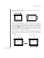
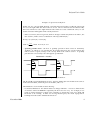
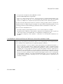
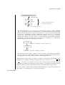
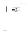
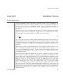
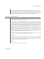
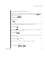
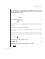
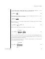
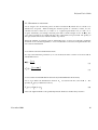
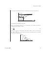
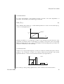
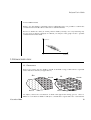
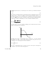
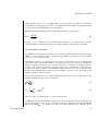
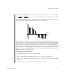
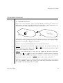
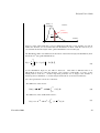
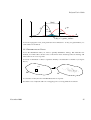
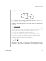
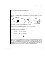
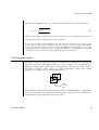
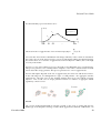
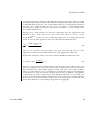
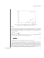
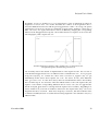
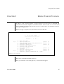
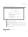
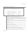
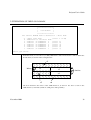
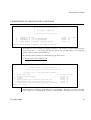
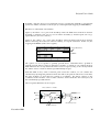
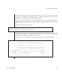
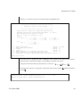
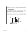
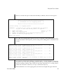
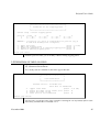
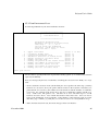
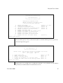
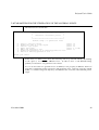
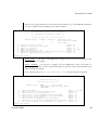
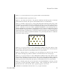
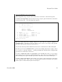
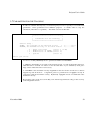
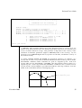
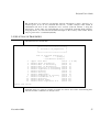
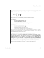
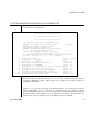
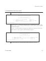
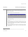
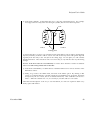
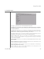
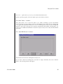
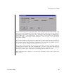
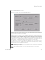
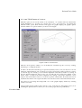
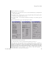
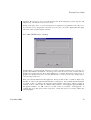
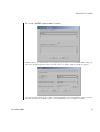
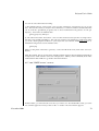
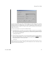
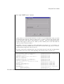
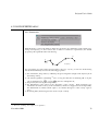
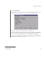
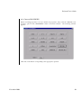

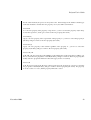
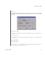
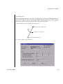
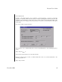
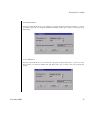
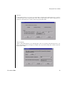
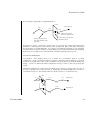
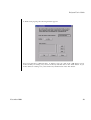
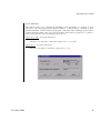
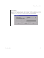
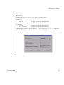
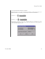
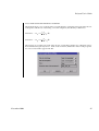
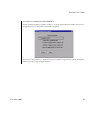
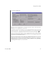
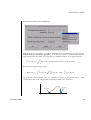
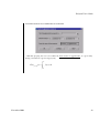
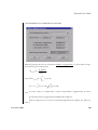
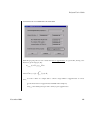
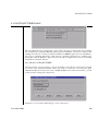
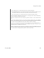
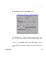
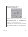
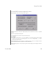
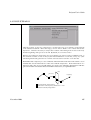
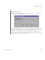
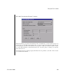
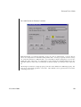
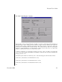
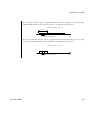
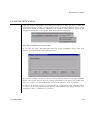
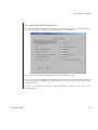
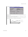
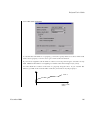
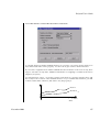
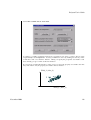
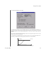
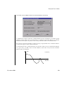
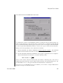
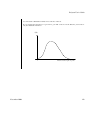
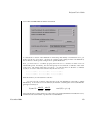
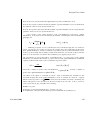
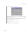
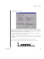
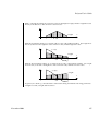
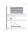
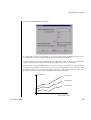
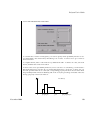
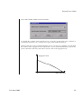
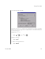
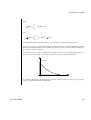
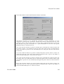
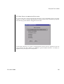
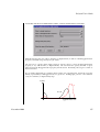
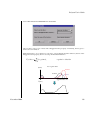
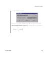
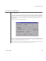
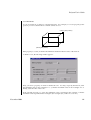





![[U4.92.04] Procédure TEST_FICHIER](http://vs1.manualzilla.com/store/data/006389562_1-6b6086926bffcd67b481cbaaace088d7-150x150.png)