Download User Manual for MetaSim V0.9.4

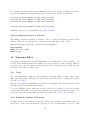
User Manual for MetaSim V0.9.4
Daniel C. Richter, Felix Ott, Alexander F. Auch, Ramona Schmid and Daniel H. Huson
February 18, 2009
Contents
Contents
1
1 Introduction
3
2 Getting Started
5
3 Obtaining and Installing the Program
5
4 Program Overview
6
4.1
General concept of MetaSim . . . . . . . . . . . . . . . . . . . . . . . . . . . . . . . .
5 Main Window
6
7
5.1
Project Tree Panel . . . . . . . . . . . . . . . . . . . . . . . . . . . . . . . . . . . . .
7
5.2
Main Panel . . . . . . . . . . . . . . . . . . . . . . . . . . . . . . . . . . . . . . . . .
8
5.3
Message Panel . . . . . . . . . . . . . . . . . . . . . . . . . . . . . . . . . . . . . . .
8
5.4
File Menu . . . . . . . . . . . . . . . . . . . . . . . . . . . . . . . . . . . . . . . . . .
8
5.5
Edit Menu . . . . . . . . . . . . . . . . . . . . . . . . . . . . . . . . . . . . . . . . . .
8
1
5.6
Database Menu . . . . . . . . . . . . . . . . . . . . . . . . . . . . . . . . . . . . . . .
9
5.7
Project Menu . . . . . . . . . . . . . . . . . . . . . . . . . . . . . . . . . . . . . . . . 10
5.8
Window Menu . . . . . . . . . . . . . . . . . . . . . . . . . . . . . . . . . . . . . . . 11
5.9
MetaSim Menu . . . . . . . . . . . . . . . . . . . . . . . . . . . . . . . . . . . . . . . 11
5.10 Tool Bar . . . . . . . . . . . . . . . . . . . . . . . . . . . . . . . . . . . . . . . . . . . 11
6 Database Functionality
11
6.1
Importing Sequence Files . . . . . . . . . . . . . . . . . . . . . . . . . . . . . . . . . 12
6.2
Structure . . . . . . . . . . . . . . . . . . . . . . . . . . . . . . . . . . . . . . . . . . 12
6.3
Searching the Database . . . . . . . . . . . . . . . . . . . . . . . . . . . . . . . . . . 13
6.4
Exporting Sequence Files . . . . . . . . . . . . . . . . . . . . . . . . . . . . . . . . . 13
7 Taxon Profiles
13
7.1
Creating Profile Files . . . . . . . . . . . . . . . . . . . . . . . . . . . . . . . . . . . . 13
7.2
Editing Profile Files . . . . . . . . . . . . . . . . . . . . . . . . . . . . . . . . . . . . 13
7.3
Profile File Format . . . . . . . . . . . . . . . . . . . . . . . . . . . . . . . . . . . . . 14
7.4
Split Abundance Value . . . . . . . . . . . . . . . . . . . . . . . . . . . . . . . . . . . 14
8 Simulation Parameter Settings
15
8.1
454 Parameter Settings
. . . . . . . . . . . . . . . . . . . . . . . . . . . . . . . . . . 15
8.2
Sanger Parameter Settings . . . . . . . . . . . . . . . . . . . . . . . . . . . . . . . . . 16
8.3
Empirical Error Model Parameter Settings . . . . . . . . . . . . . . . . . . . . . . . . 17
8.4
Exact Model Parameter Settings . . . . . . . . . . . . . . . . . . . . . . . . . . . . . 20
9 Run Simulation Window
20
10 Find Window
20
11 Population Sampler
21
11.1 Usage of Population Sampler . . . . . . . . . . . . . . . . . . . . . . . . . . . . . . . 21
11.2 Naming Convention . . . . . . . . . . . . . . . . . . . . . . . . . . . . . . . . . . . . 21
12 Taxonomy Editor
22
12.1 Usage . . . . . . . . . . . . . . . . . . . . . . . . . . . . . . . . . . . . . . . . . . . . 22
12.2 Setting the Number of Genomes . . . . . . . . . . . . . . . . . . . . . . . . . . . . . 22
12.3 File Menu Taxonomy Editor . . . . . . . . . . . . . . . . . . . . . . . . . . . . . . . . 23
2
12.4 Edit Menu Taxonomy Editor . . . . . . . . . . . . . . . . . . . . . . . . . . . . . . . 23
12.5 Select Menu Taxonomy Editor . . . . . . . . . . . . . . . . . . . . . . . . . . . . . . 23
12.6 Options Menu Taxonomy Editor . . . . . . . . . . . . . . . . . . . . . . . . . . . . . 24
12.7 View Menu Taxonomy Editor . . . . . . . . . . . . . . . . . . . . . . . . . . . . . . . 24
12.8 Toolbar Taxonomy Editor . . . . . . . . . . . . . . . . . . . . . . . . . . . . . . . . . 25
13 Command-Line Options
25
14 File Formats
28
14.1 FASTA header of Output Files . . . . . . . . . . . . . . . . . . . . . . . . . . . . . . 28
15 Examples
29
References
29
Index
31
1
Introduction
Disclaimer: This software is provided ”AS IS” without warranty of any kind. This is developmental code, and we make no pretension as to it being bug-free and totally reliable. Use at your
own risk. We will accept no liability for any damages incurred through the use of this software.
Use of the MetaSim is free, however the program is not open source.
How to cite: If you publish results obtained in part by using MetaSim , then we require that you
acknowledge this by citing the program as follows:
• D.C. Richter, F. Ott, A.F. Auch, R. Schmid and D.H. Huson, MetaSim- A Sequencing Simulator for Genomics and Metagenomics, 2008 PLoS ONE, accepted.
The research field of Metagenomics is based on the isolation and characterization of DNA from
environmental samples without the need for prior cultivation of microorganisms. In contrast to
single genome studies, analyses are applied to entire communities of microbes instead of only few
isolated organisms. It has already led to exciting insights into the ecology of different habitats.
The research field of Metagenomics is spurred by the recent development and improvement of nextgeneration sequencing technologies like Roches 454 pyrosequencing. Although these high throughput technologies promise faster and relatively inexpensive generation of reads, Sanger sequencing
still has been used in environmental genome projects to avoid the drawbacks of shorter read lengths.
The aim of MetaSim is to provide a tool for the simulation of reads based on given genome sequences
reflecting (adaptable) error models of current sequencing technologies. Additionally, the user is able
to determine the abundance of the chosen taxa. Therefore, MetaSim integrates an induced tree view
3
of the NCBI taxonomy that can be used to interactively select taxa and inner nodes of the taxonomy
to configure their relative abundances.
Another feature of MetaSim allows the user to simulate an evolved population of a single genome
sequence, using a population simulator. This feature is aimed at simulating the common real world
situation that many different, but closely related strains of a lineage coexist in the same habitat.
The resulting data sets can be used to plan and design metagenome studies and for evaluation and
improvement of metagenomic software tools and assembly algorithms.
This document provides both an introduction and a reference manual for MetaSim .
4
2
Getting Started
This section describes how to get started.
First, download an installer for the program from
www-ab.informatik.uni-tuebingen.de/software/metasim, see Section 3 for details.
Upon first startup of the program, the internal database does not contain any genome sequences. To
import the necessary files, see Section 6.1 Alternatively, to import an individual genome sequence
as (multi)fasta file use the Database→Import Files item.
Once sequences are loaded into the database, create a new project using File→New Project .
After this, the source genome sequences have to be selected for simulation. Therefore, a Taxon
Profile containing all desired sequences has to be created: Click on the Database→Show Database
to display the content of the databse in the main panel. Then select the sequence entries from the
database (Linux/Win user: left-click + hold down ctrl key, Apple Users: left-click + hold down cmd
key). Right-click on the selected entries in the database view and use the Create Taxon Profile
From Selection item. After saving the file as .mprf file, this profile is added to the Taxon Profile
folder in the Project Tree. By clicking on the taxon profile, its contents are displayed in the Main
Panel.
To start a simulation, use Project→Run Simulation to open the final configuration window.
First, select one of the available simulation setting presets (The presets can be, of course, individually adapted, refer to Section 8.) Second, choose the desired taxon profile by (un)ticking the boxes
for the listed profiles. Finally, click on the button Run Simulation to start the simulation.
After each simulation process, a new subfolder (yellow colored) is added to the project folder
containing a log file and a snapshot of the (compressed) multifasta file with the simulated reads.
The multifasta file is written into the folder where the project has been saved to.
3
Obtaining and Installing the Program
MetaSim is written in Java and requires a Java runtime environment version 1.5 or newer, freely
available from www.java.org.
MetaSim is installed using an installer program that is freely available from
www-ab.informatik.uni-tuebingen.de/software/metasim.
There are four different installers, targeting different operating systems:
• MetaSim windows 0.9.4.exe provides an installer for Windows.
• MetaSim macos 0.9.4.sit provides an installer for MacOS.
• MetaSim linux 0.9.4.rpm provides a RPM package for Linux.
• MetaSim unix 0.9.4.sh provides a shell installer for Linux, MacOS and Unix.
The executable program is called MetaSim . The unix and linux installers additionally provide
an executable called MetaSim-cmdline.
5
4
Program Overview
In this section, we give an overview of the main design goals and features of this program. Basic
knowledge of the underlying design of the program should make it easier to use the program.
MetaSim is written in the programming language Java. The advantages of this is that we can
provide versions that run under the Linux, MacOS, Windows and Unix operating systems. A
potential draw-back is that an algorithm implemented in Java will generally run slower than the
same algorithm implemented in C or C++.
The program is designed to be run in GUI mode. A Message Panel provides information about
the progress of the program. Additionally, MetaSim can be controlled from the command-line by
typing ./MetaSim cmd and using switches such as -r 5000 to set all aspects of a simulation.
Known genome sequences (fasta files) are the input for MetaSim . These source sequence are
internally stored in a database. The user then specifies the taxa composition and abundances
in a profile file or via a tree editor in GUI mode. The sampling of the reads is based on the
chosen sequencing technology and error model. Output is a collection of reads in a multifasta file
(optionally compressed). The fasta header of each read contains multiple information:
• the source genome,
• the sampled position of the reads in the source genome and
• the base positions where the read sequence was modified by the selected error model.
4.1
General concept of MetaSim
The aim of MetaSim is to provide a flexible tool, that enables the user to design several simulation
runs with e.g.
1. the same sequencing technology but with different genome sequences
2. the same sequencing technology but with different x-fold coverages
3. the same genome sequences but with different sequencing technologies
4. the same genome sequences but with different abundance values
5. etc.
For this, the overall organisation of MetaSim is based on three compounds: a database holding the
genome sequences, taxon profiles and simulation parameter settings.
The Database provides all genome sequences the user previously has to import (see Section 6).
Only those names of genome sequences present in the database can be listed in Taxon Profiles
to determine which genomes should be taken as source sequences for the simulation of reads. In
this way, the composition of metagenomes can individually be determined. See Section 7.1 to see
6
how a taxon profile is structured. A single project can contain several taxon profiles. (Prior to
simulation of a project, one is able to select the desired taxon profile(s).)
If the genome sequences in the database are assigned a unique taxonomy id (taxid) (see Section
6.1 how to import this information), the text-based taxon profile can be visualized in a Taxonomy
Editor. In this window, all taxa (genome sequences) of a single profile are visible in an induced
taxonomical tree based on the NCBI taxonomy (see Section 12).
The third compound, the configuration of Simulation Parameter Settings, is independant of
the configuration of taxon profiles. Each project comes up with four installed presets (sequencing
error models) at startup: 454, Sanger, Empirical and Exact (see Section 8). Each preset defines
several simulation parameter, such as type of sequencing technology, length of reads, mate-pair
probability, etc.. Of course, all parameter values are adaptable and new presets can be created
easily. Each project has its own set of simulation presets but one is able to export and import
selected parameter settings. More on simulation parameters can be found in Section 8.
MetaSim projects can be saved as .msim file using the File→Save As item. Parameter settings
and taxon profiles of all projects are recovered upon startup of the program.
5
Main Window
The Main Window
Message Panel.
5.1
comprises of three different panels: a
Project Tree
, a Main Panel and a
Project Tree Panel
This panel displays the database and all existing projects hierarchically in a data tree. The first
root node represents the Database. Clicking on this node will open the database view in the main
panel. If sequences are already loaded into the database, they are listed in the database table. If
projects have been already created they are listed below the database item. Each project folder
has several subfolders:
• Simulator Settings - This subfolder originally contains four simulation presets (454, Empirical, Sanger, Exact). Presets determine the simulation settings for simulation runs (sequencing
technology, parameters,... See Section 8) and can be individually adapted. Further presets
can be added by right-clicking on the Simulator Settings node and choosing Create New
Preset . This is further explained in Section 8. By clicking on a preset in the project tree,
an overview of the settings will be displayed in the Main panel.
• Taxon Profiles - In this folder, each taxon profile is listed that has been previously created.
By clicking on a profile item, the Main panel displays the content of the profile file. By
right-clicking on the Taxon Profiles node and choosing New Taxon Profile a new profile
file will be created. All existing profile files can be edited within MetaSim by clicking on the
Text Editor Button at the bottom of the Main panel. Changes are written to the file when
the Done button is clicked. More on Taxon Profile can be found in Section 7
7
• simulation run folder - After each simulation run, a result folder is created named with
the current date and time. Within this folder, a simulation log can be found which contains
information on the type of simulation, its parameters and the generated output (number
of reads created, etc.). Additionally, a snapshot of the generated multifasta file with the
resulting reads is displayed. With a left-click on this item, the first fasta entries are shown in
the Main panel.
5.2
Main Panel
The Main Panel displays information of items that have bee selected by the user in the project
tree.
5.3
Message Panel
The program writes all messages to the
Message Panel .
5.4
File Menu
The
File menu contains the following file-related items:
• The
File→New Project
• The
File→Open
• The
File→Recent Projects
item creates a new project. It is displayed in the project tree.
item provides an Open File dialog to open a MetaSim project (.msim).
item can be used to re-open a recently opened project.
• The File→Revert item can be used to revert an opened project to the saved version. This
is useful if one wants to undo changes that have been made to the project (e.g. parameter
settings).
• The
File→Save
item can be used to quick-save the current project.
• The File→Save As
location.
item can be used to save the current project assigning a name and
• The
File→Print
item is used to print the content of the Main Panel.
• The
File→Close
item is used to close a window.
• The File→Quit
MetaSim menu.
item quits the program. Under MacOS, this item is contained in the
5.5
Edit Menu
The
Edit menu contains the usual edit-related items:
• The
Edit→Cut
item is used to cut text, e.g. when editing a taxon profile.
8
• The
Edit→Copy
• The
Edit→Paste
item is used to copy text.
item is used to paste text.
• The Edit→Find item opens the Find Window which can be used to search the database,
taxon profiles and the message panel.
• The
Edit→Find Again
finds the next occurrence of a search string.
• The
Edit→Preferences
opens a submenu with the following items:
– Preferences→Set Database Location can be used to set the location of the database
to a new path in the file system. The default path is the installation directory.
– The Preferences→Set Defaults opens the simulation settings window to enable
the user to determine default values, e.g. number of reads. These values will appear for
each new simulation preset, by default.
– If the Preferences→Show Message Panel
visible, otherwise it will be hidden.
is checked the message panel will be
– The Preferences→Increase Font Size and Preferences→Decrease Font Size
items change the font size of the database. The database has to be selected first, to
enable these menu items.
• The Edit→Taxonomy Editor
profile.
• The Edit→Text Editor
Main Panel.
items open the Taxonomy Editor for a selected taxon
items open the text editor for a selected taxon profile in the
5.6
Database Menu
The
Database menu contains the following database-related items:
• The Database→Show Database
panel.
item activates the database and displays it in the main
• The Database→Import Files item opens a file dialogue to import (.gzipped ) fasta files
with genome sequences for the database (See Section 6.1).
• The Database→Remove Selected Sequences
database.
item removes selected sequences from the
• The Database→Create Taxon Profile from Selection item can be used to create a
new taxon profile based on selected entries in the database (See Section 7.1).
• The Database→Export Selected Sequences
quences into a (multi)fasta file.
item can be used to export selected se-
• The Database→Enable Selected Sequences
enables the selected sequence. Enabled
sequences are used in the process of read simulation.
9
• The Database→Disable Selected Sequences disables the selected sequence. Disabled
sequences in the database are not considered (commented out) in taxon profiles. Likewise,
they are not considered for the simulation of reads.
• The Database→Evolve Selected Sequences item opens the Population Sampler window. It can be used to generates a set of evolved (mutated) offsprings derived from the
selected sequences.
• The Database→Get Taxon IDs by GI can be used to infer taxon ids from GIs for each
existing sequence in the database. Therefore a special mapping file is needed. See Section
6.1.
• The Database→Get Taxon IDs (NCBI ftp)
can be used to infer taxon ids from a
remote file for each existing sequence in the database. Therefore a ftp network connection is
established. See Section 6.1.
• The Database→Show Hash Key
item is used to add another column to the database
named ’key’. It is the (internal,) unique key that distinguishes sequences from each other.
• The Database→Set SQL Query
query syntax. (See Section 6.3)
• The
item can be used to query the database with the standard
Database→Reset SQL Query
item resets the SQL query to:
SELECT enabled, gi, taxid, name, circular, copies, length
FROM sequences
ORDER BY name
5.7
Project Menu
The
Project menu contains the usual project-related items:
• The Project→Add Files
(multi)fasta files.
item is used to import further genome sequence files such as
• The Project→Remove Selected Files
can be used to remove selected files from a
project, such as simulation presets, taxon profiles or output folders.
• The Project→New Taxon Profile item opens a file dialogue enabling to create a new
file. A new, empty taxon profile will then be added to the Taxon Profile folder of the Project
Tree. It can be edited by any system text editor or the in-built editor of MetaSim (see Section
7.2.
• The Project→Reload Selected Profile
changed with an external text editor.
• The
Project→Rename Project
item reloads a taxon profile in case it has been
can be used to rename the project string.
• The Project→Create New Preset
item opens the simulation settings window. After
adjusting all parameters, a new preset is added to the Project Tree.
10
• The Project→Edit Selected Preset opens the simulation settings window for a selected
preset.
• The Project→Import Presets
preset.
item imports a file (.mprs) defining a simulation setting
• The Project→Export Selected Preset writes all parameters of a selected preset to a
file (.mprs). This file can be imported again by using Project→Import Presets . This can
be useful for sharing presets between different projects.
• The Project→Run Simulation
item opens the Run Simulation Window. The user
can select from the available presets and simulation settings. Finally, the simulation can be
started.
• The Project→Run With Selected Preset
item opens the Run Simulation Window.
In contrast to Project→Run Simulation the selected preset is already set.
• The Project→Run For Selected Profile
item opens the Run Simulation Window.
In contrast to Project→Run Simulation the selected taxon profile is already set.
5.8
Window Menu
• The
Window→How to cite
item gives instructions on how to cite the program.
• The Window→About item shows information about the version of MetaSim . When the
program is run under MacOS, this menu item appears in the MetaSim menu.
5.9
MetaSim Menu
Under MacOS, there is an additional, standard menu associated with the program, called the
MetaSim menu. As usual, this contains the Window→About and File→Quit menu items.
5.10
Tool Bar
The Main Window provides a tool bar containing buttons that provide short cuts to some of the
menu items associated with the window. These are the File→Open , File→Save As , Edit→Find
, and Project→Run Simulation items.
6
Database Functionality
The internal Database represents a collection of genome sequences that are available for the read
sampling. The database is based on the HSQL database engine (http://hsqldb.org/).
11
6.1
Importing Sequence Files
To start working with the program, you must first import one or more databases of genomes. Use
Database→Show Database to activate the database.
1. You can use your own ((multi)fasta) files or simply download all prokaryotic sequences from
ftp://ftp.ncbi.nlm.nih.gov/genomes/Bacteria/all.fna.tar.gz (738MB). Import your (gzip compressed) files using Database→Import Files .
2. To (additionally) work with virus sequences, in the same way download and install
ftp://ftp.ncbi.nih.gov/refseq/release/viral/viral1.genomic.fna.gz
3. For the program to function correctly,
please also download the file
ftp://ftp.ncbi.nlm.nih.gov/pub/taxonomy/gi taxid nucl.dmp.gz (345Mb) and then provide it to MetaSim using Database→Get Taxon IDs by GI . Alternatively, use the menu
item Database→Get Taxon IDs (NCBI ftp) to download and parse this file in one step.
This may take some time.
Importing the genome files has only to be done once. Imported sequences are kept in the database
even after closing the program, so they are still available when you restart MetaSim .
By default, the database is placed in the installation folder of MetaSim . You can change the
location using Edit→Preferences (Set Database Location)
6.2
Structure
To see the content of the database in the Main Panel, use Database→Show Database or click
on the Database item in the Project Tree
Several column headers are shown:
1. enabled : enables/disables a genome sequence. Only enabled sequences are used for the read
sampling.
2. gi : NCBI’s gi number of the genome sequence
3. taxid : NCBI’s taxonomy id (-1 if not assigned)
4. name: name of the organism/genome sequence
5. circular : does the sequence have a circular topology?
6. copies: copy number of the sequence
7. length: length of the sequence (base pairs)
You can click on each column header to sort the table.
To be able to use the Taxonomy Editor, each sequence should be assigned a unique taxonomy id
(6= −1). This is explained in Section 6.1.
12
6.3
Searching the Database
The database can be searched by using standard SQL syntax. For searching use Database→Set
SQL Query .
Example:
SELECT enabled, gi, taxid, name, length
FROM sequences
WHERE length > 3000000
ORDER BY length
To reset the SQL query i.e. to to see all present genome sequences in the database, use
Database→Reset SQL Query . Additionally, use the Find Window.
6.4
Exporting Sequence Files
To export sequences to (multi)fasta file(s) (.fna), select one or more entries in the database and
use the Database→Export Selected Sequences . Alternatively, right-click on the set of selected
entries and use Export Selected Sequences.
7
Taxon Profiles
A Taxon Profile determines the composition of a (metagenome) dataset that represents the set of
source genome sequences for read sampling. In a text-based profile file, each row lists one genome
sequence together with its desired abundance value.
7.1
Creating Profile Files
Profile files have the file ending .mprf and can be created and edited with any text editor. Alternatively, taxon profiles can be created within MetaSim by right-clicking on selected entries in the
database and using Database→Create Taxon Profile from Selection .
7.2
Editing Profile Files
Editing can be done with any text editor or the in-built Text Editor of MetaSim can be used.
To display the text editor in the main panel, select a taxon profile in the Project Tree and click
on the Text Editor button at the bottom-right of the main panel. All changes will be written
to the file, if one clicks on the Done button.
In case the file format (see Section 7.3) is incorrect or if the program is not able to find the mentioned
genome sequences in the dabase, the icon of the taxon profile in the Project Tree shows a Red
Exclamation Mark . Otherwise a green colored check indicates that the taxon profile is valid.
If a taxon profile has been edited with an external text editor, MetaSim has to update the file
content. For this, right-click on the concerned taxon profile and choose Reload Selected Profile .
13
7.3
Profile File Format
Each line in a taxon profile represents a single genome sequence and has the following structure:
<abundance value> <key identifier> <key value>
1. abundance value - is a relative number of arbitrary size reflecting the copy number of the
genome sequences of this specific taxon in the total taxon set.
2. key identifier - corresponds to the column names of the database suitable to identify a genome
sequence. This can be ”taxid”, ”gi” or ”name”. When using the ”name”-identifier, one is
able to use ”%” as wildcard symbol (as it is used as wildcard symbol in SQL syntax).
3. key value - the corresponding value the for chosen key identifier.
A line starting with ’#’ is treated as comment and is ignored. Here is an example for a taxon
profile.:
### MetaSim taxon profile
# 100 Methanoculleus marisnigri JR1
# 50 Alcanivorax borkumensis SK1
###
100 name "Methanoculleus marisnigri JR1"
50 name "Alcanivorax bork%"
A number of 100 genome copies (=abundance) of Methanoculleus marisnigri JR1 and 50 genome
copies of Alcanivorax borkumensis SK1 are part of this (meta)genome dataset.
If the wildcard symbol ”%” is used for a name and the database contains multiple sequences having
the same prefix, the abundance value is assigned to every genome sequence.
For example, if a line is like
50 name
"Escherichia coli%"
all available E. coli strains together with their plasmids are added to the profile with the same
abundance value 100.
7.4
Split Abundance Value
A special feature of the program is the possibility to assign abundance values not only at the species
level but also at higher taxonomical levels. The overall abundance value is shared by an arbitrary
number of sequences listed below. The syntax is:
<shared abundance value> <.>
<.> <key identifier> <key value>
<.> <key identifier> <key value>
<.> <key identifier> <key value>
#note the ’.’
#note the ’.’ at the beginning of the line
14
Here is an simplified example. The overall abundance value of 30 shall be uniformely assigned to
two genome sequences, say. .
### MetaSim taxon profile
# 30 split into:
#
15 Escherichia coli str. K12 substr. W3110
#
15 Pseudomonas aeruginosa PA7
###
30 .
. taxid 316407
. taxid 381754
The amount of 30 genome copies is split and uniformly applied to two genome sequences identified
by their taxonomic ids: Escherichia coli str. K12 substr. W3110 and Pseudomonas aeruginosa
PA7. Likewise both taxa are assigned an abundance value of 15.
This feature of a split abundance value is especially needed for the Taxonomy Editor. There, one
can assign abundance values to an inner node of the taxonomy e.g. Shewanella at genus level to
get an uniform mixture of all species in the subtree of Shewanella.
8
Simulation Parameter Settings
A preset is a configuration of simulation parameters for the generation of read sequences. MetaSim
already provides four in-built presets. Each preset determines a couple of parameters like type
of sequencing technology, mate-pair probability, error probability, read length, etc.. The current
settings of each preset (error model) are displayed in the main panel by clicking on a simulation
preset in the Project Tree. Existing presets can be individually adapted and additional presets
can be easily created by using Project→Create New Preset . To edit an existing preset, select
a preset in the project tree and use Project→Edit Selected Preset .
To interchange simulation settings between different projects, use Project→Export Selected
Preset and Project→Import Presets .
By default, MetaSim contains four different presets representing different sequencing approaches.
In the following for each preset, all parameters are described that can be adapted in the preset
configuration window. It can be opened using Project→Edit Selected Preset .
8.1
454 Parameter Settings
To simulate read sequences generated by the pyrosequencing approach (Roche’s 454).
• Primary Configuration
Preset Name : Title of preset
Number of Reads or Mate Pairs : Number of read sequences to generate. x mate-pairs
means 2x reads.
Error Model : 454/Empirical/Sanger/Exact
15
DNA Clone Size Distribution Type : Uniform/Normal: A Clone in MetaSim is a DNA
fragment that is randomly extracted from the source genome sequence for read/mate-pair
sampling. Selection how the length of the clone is distributed.
Mean : Mean length of clone. For Sanger sequencing, this length defines the mate-pairs
length.
Second Parameter : standard deviation of clone length.
• Error Model Configuration
Expected Read Length : Read sequence length in bp. This value depends on/affects the
number of Flow Cycles .
Number of Flow Cycles : This value depends on/affects the read length.
Mate Pair Probability : Value betw. 0 and 1. 0 means: no mate-pair.
Mate Pair Read Length : Determines the length of both reads of a mate pair.
Remove Linker Sequence From Output : Originally, 454 mate pairs include a 44bp
linker sequence. If checked, MetaSim writes both mates (reads) separately in the output file
without any linker sequence. If unchecked, the linker sequence will be written to the fasta
file as well. In the latter case, a mate pair is written into a single fasta entry.
Mean Negative Flow Signal
: A negative flow is a flow of nucleotides in which the
sequence to synthesize is not elongated. Light intensities of negative flows follow a lognormal
distribution N (µ, k · µ). The default value (µ = 0.23) is taken from [1]
Std. Deviation for Negative Flow Signals : The default value (k = 0.15) is taken
from [1]
Signal Std. Deviation Multiplier : The default value (0.15) is taken from [1]
Scale Standard Deviation with Square Root of Mean
: If checked the standard
√ deviation of the light intensity emitted grows with square root of µ, i.e. N µ, k · µ
Generate Signal Trace : If checked, the algorithm generates a signal trace. This does
not affect the results. Currently, the signal trace is only used internally.
• Simulator Options
Number of Threads : In case of running MetaSim on a multiprocessor machine, select
the number of threads to distribute the computation.
Generate FASTA Output : If unchecked, the program will just simulate the generation
of reads without writing results to a file. The result log displays the simulation results.
Compress Output (gzip) : Automatically compresses the multifasta file using gzip.
Use Uniform Sequence Weights : If unchecked, disables weighting of sequences by
sequence length and number of per-genome copies.
Merge All Files Into a Single Taxon Profile : If checked, merge all files in the profile
folder into a single taxon profile. Output will be one multifasta file. If unchecked, output
will be one multifasta file per taxon profile.
8.2
Sanger Parameter Settings
• Primary Configuration
see Primary Configuration of 454 parameter settings.
16
• Error Model Configuration
Read Length Distribution : Normal/Uniform Distribution of read sequence length
Mean: Mean length of read sequence.
Second Parameter: Standard deviation of mean read length.
Mate Pair Probability: Value betw. 0 and 1. 0 means: no mate-pair.
Error Rate at Read Start : Value between 0.00 and 1.00
Error Rate at Read End : Value between 0.00 and 1.00
Insertion Error Rate : Value between 0.00 and 1.00.
Deletion Error Rate : Value between 0.00 and 1.00.
• Simulator Options
see Simulator Options of 454 parameter settings.
8.3
Empirical Error Model Parameter Settings
As an additional feature, MetaSim includes an Empirical Error Model that allows the incorporation of user-defined error statistics for the generation of read sequences. As default configuration,
the programs comes with an error model based on Illumina’s sequencing technology . This error
model is derived from empirical studies. It is based on mappings (error curves) that assign error
rates to base positions (see Fig. 1 for an example).
Figure 1: Probability curve of substition errors for 36bp reads. x-axis: read position, y-axis: error
rate.
Each mapping has three parameters (the last two are optional):
• type of error,
• base at position where the error occurs and
17
• base preceding the position where the error occurs.
In addition, in case of a substitution error the user can specify the probability of integrating a
particular base depending on the type of the base at the error positions and the preceding base.
Instructions for creating individual Empirical Error Models
An empirical error model is a text-based file (.mconf ). It can be created with any text editor.
Lines starting with ’#’ are ignored. There is only one file for all error model settings.
First of all, the Base Substitution Rate
can be defined.
# [<preceding base>](<from>,<to>) <value>
# "[]" marks optional parameters.
# (Set switch rates for A following G)
G(A,T) 0.4
G(A,C) 0.3
G(A,G) 0.3
# (Alternatively, set switch rates for all C)
(C,T) 0.3
(C,A) 0.3
(C,G) 0.4
Further, the Empirical Error Rates can be defined in the same file.
The specification of error curves is done by listing the probability values row-wise per base position.
E.g. for a 35bp read, 35 probability values have to listed. The header of such a list must contain
one type of error: SUBSTITUTION ERROR, INSERTION ERROR or DELETION ERROR. In that case, all
bases (A,T,G,C) receive equal error rates. For example:
# <error type>
# Set all substitution rates
SUBSTITUTION_ERROR
0.00606508512067950
first base ...
0.00675296642376962
...
0.05190994307855664
... last base
If one wishes to assign error rates to a specific base one can use:
# <error type> [(<base>)]
# "[]" marks optional parameters.
# Set insertion rates for every A
INSERTION_ERROR (A)
0.00606508512067950
first base ...
0.00675296642376962
18
...
0.05190994307855664
... last base
Additonally, one can define error rates for a specific base that is preceeded by another base. For
example:
# <error type> [<preceding base>] [(<base>)]
# "[]" marks optional parameters.
# Set substitutions rates for a G following an A
SUBSTITUTION_ERROR A(G)
0.00606508512067950
first base...
0.00675296642376962
...
0.05190994307855664
... last base
Likewise 48 mappings are possible to create.
Note: In case an equal mapping has been defined before in the file, only the last one is considered.
This can be useful, if, first, SUBSTITUTION ERROR defines a default substitution rate for all bases
and then SUBSTITUTION ERROR X(Y) specifies error rates for base Y following base X.
Settings in configuration Window
Once, all error probabilities are listed in a .mconf file, this file can be loaded into MetaSim .
• Primary Configuration
see Primary Configuration of 454 parameter settings.
• Error Model Configuration
Click the Load button to import an error model (text-based file, ending .mconf ). After the
import, the main header that are defined in the error model are summarized and displayed
in the text box below. (For an example load the default error model based on Illumina reads
(36bp) by choosing the file illumina-error-model.mconf in the examples folder.
• Simulator Options
see Simulator Options of 454 parameter settings.
Outlook
Due to its abstract definition, the empirical error model is suitable for integrating upcoming sequencing technologies. We are very interested in further empirical models of other technologies. If
you like to provide your error models, send them to [email protected]. We will
provide them on our MetaSim homepage for other users.
19
8.4
Exact Model Parameter Settings
The Exact Error Model is suitable for sampling reads without modifying any bases, i.e. in
contrast to the other provided error models, no substitution, insertion or deletion will be applied
to the read sequences.
• Primary Configuration
see Primary Configuration of 454 preset.
• Simulator Options
see Simulator Options of 454 preset.
9
Run Simulation Window
The Run Simulation Window opens if the user clicks on the Run Simulation button or by
using Project→Run Simulation .
Before a simulation run, the user has to configure which simulation settings and which taxon profiles
should be used. The settings can be chosen from the pull-down menu. Additionally, all marked
taxon profiles are used for the simulation. Note that it depends on the setting Merge All Files Into
a Single Taxon Profile whether the reads of all marked taxon profiles are merged together into one
multifasta file or not.
If the simulation has been successful, a new result folder is created within the Project Tree.
10
Find Window
The Find Window can be opened using the Edit→Find item. Its purpose is to find sequence
entries in the internal database or any text in the simulator settings, taxon profiles and the message
panel. Depending on the current view in the Main Panel, the user can select from different targets
in the Find window. A target is a panel that can be searched.
Use the following check boxes to parametrize the search:
• If the Whole Words Only item is selected, then only strings matching the complete query
string will be returned.
• If the Case Sensitive
parisons.
item is selected, then the case of letters is distinguished in com-
• If the Regular Expression item is selected, then the query is interpreted as a Java regular
expression.
• If the
Forward item is selected, the search proceeds in forward direction.
• If the
Backward item is selected, the search proceeds in backward direction.
20
• If the
Global
• If the
forward item is selected, the search scope comprises only the selected text.
item is selected, the search scope comprises all contained text.
Press the Close, First or Next buttons to close the dialog, or find the first, or next occurrence of
the query, respectively. Press the Find All button to find all occurrences of the query.
11
Population Sampler
MetaSim includes a Population Sampler that optionally generates a set of evolved (mutated)
offsprings derived from single source genomes, using a given evolutionary tree.
This tree describes how the offspring sequences descend from the source sequence. By default, a
random pyholgenetic tree is generated under the Yule-Harding model [?, ?], but alternatively,
user-defined trees can also be loaded.
As a simple model of DNA evolution, the Jukes-Cantor formula is applied to estimate a probability
of change for each base pair, with a customizable transition rate α (0.001 by default) and time t
based on the edge weights. MetaSim then generates the designated number of evolved genomes and
then adds them to the internal genome database.
11.1
Usage of Population Sampler
To generate a set of offsprings for a single genome sequence, select a sequence in the database and
use Database→Evolve Selected Sequences . The population sampler window will appear with
the following parameter settings:
• Tree File
The user can import his own tree file. The Yule-Harding tree is loaded by default.
• Number of Leaves
Determines the number of leaves (amount of desired offspring sequences).
• Jukes-Cantor Model Alpha
Transition rate α. (default: 0.001)
After clicking on the Evolve Button , MetaSim generates the desired number of new (mutated)
genome sequences ( Offsprings ). These offsprings are added to the database directly following the
source sequence entry. To export the generated offspring sequences, one can use Database→Export
Selected Sequences .
11.2
Naming Convention
Offspring sequences have the following naming convention.
The name of their original sequences their name is taken and automatically extended with two
additional tags: an (ascending)offspring id and an artificial taxid.
21
For example, if Acaryochloris marina MBIC11017 is the source genome and the user decides to
generate 100 offsprings, the final offspring sequence names in the database look like this:
Acaryochloris
Acaryochloris
Acaryochloris
...
Acaryochloris
marina MBIC11017 {OFF_0001}[taxon0006]
marina MBIC11017 {OFF_0002}[taxon0003]
marina MBIC11017 {OFF_0003}[taxon0010]
marina MBIC11017 {OFF_0100}[taxon0087]
Offspring sequences are not visualized in the Taxonomy Editor.
Selecting Offspring Sequences in Database
The naming convention is useful if one wishes to remove or disable all offspring sequences in the
database. Therefore, the SQL query tool ( Database→Set SQL Query ) can be used:
SELECT enabled,gi,taxid,name,circular,copies,length,key
FROM SEQUENCES
WHERE name like ’%OFF%’
ORDER BY name
12
Taxonomy Editor
To facilitate the design of taxon profiles, MetaSim provides an interactive Taxonomy Editor . It
is based on the NCBI taxonomy and visualizes every species (genome sequence from the database)
as a leaf in a tree. Genome sequences in the database must be assigned a taxon id. Otherwise the
taxonomy editor will not work properly.
12.1
Usage
The Taxonomy Editor window is opened using the Taxonomy Editor button on the bottomright of the main panel. This button is enabled if the user has selected a (empty) taxon profile
from the Project Tree.
Once the taxonomy editor is initialized, a taxonomic tree is displayed embedding all sequences with
an unique taxon id from the internal database.
To set the abundance values, right-click on a node and select Set Number of Genomes from the
context menu. After that, one can save these settings to the current (opened) taxon profile or one
can create a new taxon profile. After the saving, the profile in the Project Tree is updated.
12.2
Setting the Number of Genomes
By using Options→Set Number of Genomes the user can determine the abundance value of a
specific node or leaf of the taxonomy tree (Can also be done by right-clicking on a node.). This
22
number equals the value defined in the text-based taxonomy profile for each genome sequence. The
higher this value, the bigger the node/leaf is displayed in the tree.
A useful feature is to assign such a value to an inner node instead to a leaf (=specific genome
sequence) of the taxonomy. Section 7.4 explains this in more detail.
12.3
File Menu Taxonomy Editor
• The
File→Open Taxonomy Editor
• The
File→Save Taxonomy Profile
item opens an existing taxon profile (.mprf ).
item (quick-)saves the current taxon profile).
• The File→Save Taxonomy Profile As
file).
item saves the current taxon profile to a (.mprf -
• The File→Export Image item can be used to export the current view to a graphics file
(e.g. .eps, .gif, .jpg, .png, .svg, .bmp, .pdf ).
• The File→Print item is used to print the current view.
• The File→Close item is used to close the taxonomy window without quitting MetaSim .
• The File→Quit item quits the MetaSim . Under MacOS, this item is contained in the
MetaSim menu.
12.4
Edit Menu Taxonomy Editor
• The Edit→Copy item is used to copy text e.g. nodes labels.
• The Edit→Find item opens the Find Window.
• The Edit→Find Again finds the next occurrence of a search string.
• The Edit→Format
width of edges, etc.).
12.5
The
can be used to format selected tree items (e.g. size, color of nodes,
Select Menu Taxonomy Editor
Select menu contains items for selecting different sets of substructures of the tree.
• The
Select→Select All
• The
Select→Select Nodes
item is used to select all nodes.
• The
Select→Select Edges
item is used to select all edges.
• The Select→Deselect All
currently selected.
item is used to select all nodes, edges and labels.
item is used to deselect all nodes, edges and labels that are
23
• The Select→Deselect Nodes
selected.
item is used to deselect all nodes that are currently
• The Select→Deselect Edges item is used to deselect all edges that are currently selected.
• The
Select→Select Leaves
• The
Select→Select Subtree
• The
Select→Invert Selection
• The
Select→Scroll to Selection
• The
Select→List Selected Taxa
12.6
The
item is used to select all leaves with their labels.
item is used to select a subtree of a selected inner node.
item is used to invert the current selection.
item is used to scroll to the current selection.
item is used to list all selected taxa.
Options Menu Taxonomy Editor
Options menu contains items for (un)collapsing nodes and subtrees.
• The
Options→Collapse
• The
Options→Uncollapse
item enables to collapse a subtree at a selected specified node.
item is used to uncollapse (expand) the whole tree.
• The Options→Uncollapse Subtree
collapsed subtree.
item is used to uncollapse (expand) a selected,
• The Options→Collapse Complement
currently selected part of the tree.
item is used to collapse all subtrees except the
• The Options→Collapse at Level
level from the root.
item is used to collapse all subtrees at the specified
• The Options→Set Number of Genomes
can be used to set the abundance value (copy
number) of a specific node (see Section 12.2).
12.7
View Menu Taxonomy Editor
The Views
labels.
menu contains items for scaling the tree, using the magnifier and showing/hiding
• The
View→Zoom to Fit
• The
View→Fully Contract
• The
View→Fully Expand
• The
View→Use Magnifier
• The
View→Show Node Labels
item is used to make all node labels visible.
• The
View→Hide Node Labels
item is used to hide all node labels.
item is used to scale the tree to fit the window.
item is used to contract the tree.
item is used to expand the whole tree.
item is used to turn the magnifier functionality on and off.
24
• The
View→Show Edge Labels
item is used to make edge labels visible.
• The
View→Hide Edge Labels
item is used to hide edge labels.
• The View→Sparse Labels item instructs the program to show only a subset of the taxon
labels, thus avoiding overlapping labels.
12.8
Toolbar Taxonomy Editor
For easier access of frequently used functions, a Toolbar is provided with the following functions:
• File→Print ,
• File→Export Image , Edit→Format
• The
Expand view vertically button expands the tree vertically.
• The
Contract view vertically button shrinks the tree vertically.
• The
Expand view horizontally button expands the tree horizontally.
• The
Contract view horizontally button shrinks the tree horizontally.
• View→Zoom to Fit ,
• View→Fully Contract ,
• View→Fully Expand ,
• View→Use Magnifier ,
• Edit→Find .
13
Command-Line Options
As an alternative to the graphical user interface, MetaSim can be controlled via command line mode.
Therefore, naviagate to the MetaSim installation folder and execute ./MetaSim cmd <option(s).
The MetaSim program is controlled by options. Here we list all available options. Use the -h option
to obtain a listing of all options command line options directly from the program.
Here is an example:
MetaSim cmd -mg /usr/local/metasim/examples/errormodel.mconf -r10000
/usr/local/metasim/examples/example-profile1.mprf
The previous example means: start MetaSim in command line mode. Use the empirical error model
with a specified error model config file. Generate 10000 reads and use the specified taxon profile
(alternatively provide a fasta file with a single genome sequence. Then MetaSim uses only this
genome to sample the reads from).
25
-r, --reads VALUE
Set the number of
5000).
reads to
generate
(default:
-f, --clones-mean VALUE
Sets the mean value of the fragment
(default: Error model dependent).
lengths
-t, --clones-param2 VALUE
Sets the second parameter (std./max. deviation)
of the fragment length distribution (default:
Error model dependent).
-v, --uniform-clones
Use a uniform
fragment
length distribution
instead of gaussian.
-4, --454
Apply the 454 error model to the generated reads.
--454-cycles VALUE Sets the number of cycles (454 error model,
default: 99).
--454-mate-probability VALUE
Sets the probability of paired
model, default: 0.0).
reads (454 error
--454-paired-read-length VALUE
Sets the read length for paired reads (454 error
model, default: 20).
--454-remove-linker
--454-nosqrt
remove linker sequence from paired reads (454
error model).
Signal distributions: "stddev=k*mean" instead of
"stddev=k*sqrt(mean)" (454 error model).
--454-multiplier VALUE
Sets the proportionality constant for computation
of signal std. deviations (454 error model,
default: 0.15).
--454-logn-mean VALUE
Sets the mean of the lognormal negative flow
signal distribution (454 error model, default:
0.23).
--454-logn-std VALUE
Sets the std. deviation of the lognormal negative
flow signal distribution (454
error model,
default: 0.15).
26
--454-trace
--sanger
Use an explicit signal trace (454 error model).
Apply the sanger error model to the generated
reads.
--sanger-mean VALUE
Sets the mean value
(default: 1000.0)
for
sanger
read
lengths
--sanger-param2 VALUE
Sets the second parameter (std./max. deviation)
of the sanger read length distribution (default:
100.0)
--sanger-uniform
Use a uniform read length distribution for sanger
reads.
--sanger-err-start VALUE
Sets the initial error rate for the sanger error
model (default: 0.01).
--sanger-err-end VALUE
Sets the final error rate for the
model (default: 0.02).
sanger
--sanger-deletions VALUE
Sets the relative deletion rate for the
error model (default: 0.2).
error
sanger
--sanger-insertions VALUE
Sets the relative insertion rate for the sanger
error model (default: 0.2).
-m, --empirical
Apply the empirical/solexa error model to the
generated reads.
-g, --empirical-cfg VALUE
Specify an empirical error model config file.
-a, --add-files
Add the provided fastA files to the database.
--add-archives
Add fastA files from .tar.gz archives to the
database.
--test-db
Test the database integrity.
--description VALUE
--length VALUE
Print out the description of sequences where the
hash string starts with VALUE.
Print out the length of sequences where the hash
string starts with VALUE
27
--taxupdate VALUE
-x, --print-taxids
-c, --combine
--uniform-weights
--threads VALUE
-z, --compress
-q, --no-progress
--seed VALUE
-d, --output-dir VALUE
Update taxon ids from a sorted and gzip’ed
gi-to-taxon-id map file.
print a sorted list of all taxon ids present in
the database
Combine all files to a single simulation.
Do not weight sequences by size and number of
per-genome copies.
Set number of readsim threads. ‘0’ runs in serial
mode (default 1).
Compress output.
Suppress all progress information.
Sets the random seed. To obtain reproducible
results, threading must also be disabled.
Specify the output directory
-s, --simple-output-name
Don’t hash string in name of output file
-h, --help
Display this help and exit.
-stop processing commandline options
14
File Formats
MetaSim uses and produces three file formats:
• .msim : This is the main Project File (XML format) that saves all necessary information
about a project such as simulation presets, contained taxon profiles and log files.
• .mprf : Files having such an ending are Taxon Profile files. It determines the composition
and abundance of selected taxa.
• .mconf : These files are used to define individual Empirical Error Models.
14.1
FASTA header of Output Files
Output of MetaSim are multifasta files with the generated read sequences. To be able to trace back
a read (source genome, sampling position, insertion of errors), all fasta headers contain multiple
information separated by ”|”.
r<nr of read >.<index >
|SOURCES={GI=<gi number>, <backward (bw) or forward (fw) read>, <sample
position> }
|ERRORS=<list of generated base errors>
|SOURCE 1="<name of genome> " <MetaSim’s hash key of source sequence in database>
Here is an example (split into several lines for better overview):
>r30.1
28
|SOURCES={GI=49474831,bw,494076-494112}
|ERRORS={33:G,40 1:C,43 2:G,53:-}
|SOURCE 1="Bartonella henselae str.Houston-1" (6044c4ffa5bc1b2f851929708279679ab66dcc19)
The list of inserted errors contains a single, comma-separated entry for every error. The base
positions refer to the sampled and unmodified read sequence. The symbol ” ” represents insertions,
the symbol ”-” represents deletions. The remaining entries are substitutions. Referring to the
mentioned example, read r30.1 has been sampled from the B. henselae str.Houston-1 strain with
gi number 49474831 from the base positions 494076-494112. It has been sampled as a single
backward read (mate pairs consist of two indeces x.1 and x.2).
The read has been modified:
At position 30 the base has been substituted with a ’G’.
At position 40 one ’C’ has been added.
At position 43 two ’G’ have been added.
The base at position 53 has been deleted.
15
Examples
Example files are provided with the program. They are contained in the examples sub directory
of the installation directory. The precise location of the installation directory depends upon your
operating system.
• illumina-error-model.mconf:
This file contains the empirical error model for the Illumina Sequencing Technology (for a
read length of 36bp). It can be loaded if the Empirical Error Model is chosen as simulation
preset.
• example-taxon-profile1.mprf:
This is a really simple taxon profile. It contains only four entries demonstrating the structure
of a typical taxon profile.
• example-taxon-profile2.mprf:
A taxon profile containing 11 diverse taxa from many different phylae.
• example project 1.msim:
An example project.
Note: To be able to generate reads with these example profiles, the user first has to fill the
database with the appropriate genome sequences. Our recommendation is to download the file
with all available genome sequences from the NCBI homepage (see Section 6.1).
References
[1] M. Margulies, M. Egholm, W.E. Altman, S. Attiya, J.S. Bader, L.A. Bemben, J. Berka, M.S.
Braverman, Y.-J. Chen, Z. Chen, S.B. Dewell, L.D., J.M. Fierro, X.V. Gomes, B.C. Godwin,
29
W. He, S. Helgesen, C.H. Ho, G.P. Irzyk, S.C. Jando, M.L.I. Alenquer, T.P. Jarvie, K.B.
Jirage, J.-B. Kim, J.R. Knight, J.R. Lanza, J.H. Leamon, S.M. Lefkowitz, M. Lei, J. Li, K.L.
Lohman, H. Lu, V.B. Makhijani, K.E. McDade, M.P. McKenna, E.W. Myers, E. Nickerson, J.R.
Nobile, R. Plant, B.P. Puc, M.T. Ronan, G.T. Roth, G.J. Sarkis, J.F. Simons, J.W. Simpson,
M. Srinivasan, K.R. Tartaro, A. Tomasz, K.A. Vogt, G.A. Volkmer, S.H. Wang, Y. Wang,
M.P. Weiner, P. Yu, R.F. Begley, and J.M. Rothberg. Genome sequencing in microfabricated
high-density picolitre reactors. Nature, 437(7057):376–380, 2005.
30
Index
-h, 25
./MetaSim cmd ¡option(s), 25
.mconf, 28
.mprf, 28
.msim, 28
¿r30.1 , 28
#, 18
%, 14
100, 14
A,T,G,C, 18
About, 11
Acaryochloris marina MBIC11017, 22
Add Files, 10
Database→Reset SQL Query, 10, 13
Database→Set SQL Query, 10, 13, 22
Database→Show Database, 5, 9, 12
Database→Show Hash Key, 10
Decrease Font Size, 9
Deletion Error Rate, 17
DELETION ERROR, 18
Deselect All, 23
Deselect Edges, 24
Deselect Nodes, 24
Disable Selected Sequences, 10
Disclaimer, 3
DNA Clone Size Distribution Type, 16
edge labels, 25
Edit, 8
Backward, 20
Edit Selected Preset, 11, 15
Base Substitution Rate, 18
Edit→Copy, 9, 23
Edit→Cut, 8
Case Sensitive, 20
Edit→Find, 9, 11, 20, 23, 25
Close, 8, 21, 23
Edit→Find Again, 9, 23
Collapse, 24
Edit→Format, 23, 25
Collapse at Level, 24
Edit→Paste, 9
Collapse Complement, 24
Edit→Preferences, 9, 12
command line options, 25
Edit→Taxonomy Editor, 9
Compress Output (gzip), 16
Edit→Text Editor, 9
Contract view horizontally, 25
Empirical Error Model, 17
Contract view vertically, 25
Empirical Error Rates, 18
Copy, 9, 23
Enable Selected Sequences, 9
Create New Preset, 7, 10, 15
Error Model, 15
Create Taxon Profile From Selection, 5
Error Model Configuration, 16
Create Taxon Profile from Selection, 9, 13
Error Rate at Read End, 17
Cut, 8
Error Rate at Read Start, 17
Database, 9, 11
Evolve Button, 21
Database→Create Taxon Profile from Selection, Evolve Selected Sequences, 10, 21
9, 13
Exact Error Model, 20
Database→Disable Selected Sequences, 10
example-taxon-profile1.mprf, 29
Database→Enable Selected Sequences, 9
example-taxon-profile2.mprf, 29
Database→Evolve Selected Sequences, 10, 21
example project 1.msim, 29
Database→Export Selected Sequences, 9, 13, 21 examples, 29
Database→Get Taxon IDs (NCBI ftp), 10, 12
Expand view horizontally, 25
Database→Get Taxon IDs by GI, 10, 12
Expand view vertically, 25
Database→Import Files, 5, 9, 12
Expected Read Length, 16
Database→Remove Selected Sequences, 9
Export Image, 23, 25
31
Export Selected Preset, 11, 15
Export Selected Sequences, 9, 13, 21
interchange simulation settings, 15
Invert Selection, 24
File, 8
File→Close, 8, 23
File→Export Image, 23, 25
File→New Project, 5, 8
File→Open, 8, 11
File→Open Taxonomy Editor, 23
File→Print, 8, 23, 25
File→Quit, 8, 11, 23
File→Recent Projects, 8
File→Revert, 8
File→Save, 8
File→Save As, 7, 8, 11
File→Save Taxonomy Profile, 23
File→Save Taxonomy Profile As, 23
Find, 9, 11, 20, 23, 25
Find Again, 9, 23
Find All, 21
Find Window, 20
First, 21
Flow Cycles, 16
Format, 23, 25
Forward, 20
forward, 21
Fully Contract, 24, 25
Fully Expand, 24, 25
Jukes-Cantor Model Alpha, 21
Generate FASTA Output, 16
Generate Signal Trace, 16
Get Taxon IDs (NCBI ftp), 10, 12
Get Taxon IDs by GI, 10, 12
gi, 14
Global, 21
Hide Edge Labels, 25
Hide Node Labels, 24
How to cite, 3, 11
Illumina’s sequencing technology, 17
illumina-error-model.mconf, 19, 29
Import Files, 5, 9, 12
Import Presets, 11, 15
Increase Font Size, 9
Insertion Error Rate, 17
INSERTION ERROR, 18
key, 10
Linux, 5, 6
List Selected Taxa, 24
Load, 19
MacOS, 5, 6
Main Panel, 8
Main Window, 7
Mate Pair Probability, 16
Mate Pair Read Length, 16
Mean, 16
Mean Negative Flow Signal, 16
Merge All Files Into a Single Taxon Profile, 16
Message Panel, 8
MetaSim, 11
MetaSim-cmdline, 5
MetaSim linux 0.9.4.rpm, 5
MetaSim macos 0.9.4.sit, 5
MetaSim unix 0.9.4.sh, 5
MetaSim windows 0.9.4.exe, 5
name, 14
New Project, 5, 8
New Taxon Profile, 7, 10
Next, 21
Node→Create New Preset, 7
Node→New Taxon Profile, 7
Number of Flow Cycles, 16
Number of Leaves, 21
Number of Reads or Mate Pairs, 15
Number of Threads, 16
Offsprings, 21
Open, 8, 11
Open Taxonomy Editor, 23
Options, 24
Options→Collapse, 24
Options→Collapse at Level, 24
Options→Collapse Complement, 24
Options→Set Number of Genomes, 22, 24
Options→Uncollapse, 24
32
Options→Uncollapse Subtree, 24
Paste, 9
Population Sampler, 21
Preferences, 9, 12
Preferences→Decrease Font Size, 9
Preferences→Increase Font Size, 9
Preferences→Set Database Location, 9
Preferences→Set Defaults, 9
Preferences→Show Message Panel, 9
preset configuration, 15
Preset Name, 15
Primary Configuration, 15
Print, 8, 23, 25
Project, 10
Project File, 28
Project Tree, 7
Project→Add Files, 10
Project→Create New Preset, 10, 15
Project→Edit Selected Preset, 11, 15
Project→Export Selected Preset, 11, 15
Project→Import Presets, 11, 15
Project→New Taxon Profile, 10
Project→Reload Selected Profile, 10
Project→Remove Selected Files, 10
Project→Rename Project, 10
Project→Run For Selected Profile, 11
Project→Run Simulation, 5, 11, 20
Project→Run With Selected Preset, 11
Quit, 8, 11, 23
r30.1, 29
r¡nr of read ¿.¡index ¿, 28
Read Length Distribution, 17
Recent Projects, 8
Red Exclamation Mark, 13
Regular Expression, 20
Reload Selected Profile, 10, 13
Remove Linker Sequence From Output, 16
Remove Selected Files, 10
Remove Selected Sequences, 9
Rename Project, 10
Reset SQL Query, 10, 13
Revert, 8
Run For Selected Profile, 11
Run Simulation, 5, 11, 20
Run Simulation Window, 20
Run With Selected Preset, 11
Save, 8
Save As, 7, 8, 11
Save Taxonomy Profile, 23
Save Taxonomy Profile As, 23
Scale Standard Deviation with Square Root of
Mean, 16
Scroll to Selection, 24
Second Parameter, 16
Select, 23
Select All, 23
Select Edges, 23
Select Leaves, 24
Select Nodes, 23
Select Subtree, 24
Select→Deselect All, 23
Select→Deselect Edges, 24
Select→Deselect Nodes, 24
Select→Invert Selection, 24
Select→List Selected Taxa, 24
Select→Scroll to Selection, 24
Select→Select All, 23
Select→Select Edges, 23
Select→Select Leaves, 24
Select→Select Nodes, 23
Select→Select Subtree, 24
Set Database Location, 9
Set Defaults, 9
Set Number of Genomes, 22, 24
Set SQL Query, 10, 13, 22
Show Database, 5, 9, 12
Show Edge Labels, 25
Show Hash Key, 10
Show Message Panel, 9
Show Node Labels, 24
Signal Std. Deviation Multiplier, 16
Simulator Options, 16
Sparse Labels, 25
Std. Deviation for Negative Flow Signals, 16
SUBSTITUTION ERROR, 18, 19
SUBSTITUTION ERROR X(Y), 19
taxid, 14
33
Taxon Profile, 13
Taxonomy Editor, 9, 22
Text Editor, 9, 13
Toolbar, 25
Tree File, 21
Uncollapse, 24
Uncollapse Subtree, 24
Unix, 5, 6
Use Magnifier, 24, 25
Use Uniform Sequence Weights, 16
View→Fully Contract, 24, 25
View→Fully Expand, 24, 25
View→Hide Edge Labels, 25
View→Hide Node Labels, 24
View→Show Edge Labels, 25
View→Show Node Labels, 24
View→Sparse Labels, 25
View→Use Magnifier, 24, 25
View→Zoom to Fit, 24, 25
Views, 24
Whole Words Only, 20
Window→About, 11
Window→How to cite, 11
Windows, 5, 6
X, 19
x.1, 29
x.2, 29
Y, 19
Yule-Harding, 21
Zoom to Fit, 24, 25
34