1
Combined Platform for Boost Guidance
and Attitude Control for Sounding
Rockets
Examensarbete utfört i Reglerteknik
vid Tekniska Högskolan i Linköping
av
Per Abrahmsson
Reg nr: LiTH-ISY-EX-3479-2004
Linköping 2003
Combined Platform for Boost Guidance
and Attitude Control for Sounding
Rockets
Examensarbete utfört i Reglerteknik
vid Tekniska Högskolan i Linköping
av
Per Abrahmsson
Reg nr: LiTH-ISY-EX-3479-2004
Supervisors: Albert Thuswaldner
David Lindgren
Examiner: Anders Helmersson
Linköping 26th February 2004.
Avdelning, Institution
Division, Department
Datum
Date
2004-02-25
Institutionen för systemteknik
581 83 LINKÖPING
Språk
Language
Svenska/Swedish
X Engelska/English
Rapporttyp
Report category
Licentiatavhandling
X Examensarbete
C-uppsats
D-uppsats
ISBN
ISRN LITH-ISY-EX-3479-2004
Serietitel och serienummer
Title of series, numbering
ISSN
Övrig rapport
____
URL för elektronisk version
http://www.ep.liu.se/exjobb/isy/2004/3479/
Titel
Title
Kombinerad Plattform för Ban- och Attiydstyrning av Sondraketer
Combined Platform for Boost Guidance and Attitude Control for Sounding Rockets
Författare
Author
Per Abrahamsson
Sammanfattning
Abstract
This report handles the preliminary design of a control system that includes both attitude control
and boost control functionality for sounding rockets. This is done to reduce the weight and volume
for the control system. A sounding rocket is a small rocket compared to a satellite launcher. It is
used to launch payloads into suborbital trajectories. The payload consists of scientific experiments,
for example micro-gravity experiments and astronomic observations. The boost guidance system
controls the sounding rocket during the launch phase. This is done to minimize the impact
dispersion. The attitude control system controls the payload during the experiment phase. The
system that is developed in this report is based on the DS19 boost guidance system from Saab
Ericsson Space AB. The new system is designed by extending DS19 with software and hardware.
The new system is therefore named DS19+. Hardware wise a study of the mechanical and electrical
interfaces and also of the system budgets for gas, mass and power for the system are done to
determine the feasibility for the combined system. Further a preliminary design of the control
software is done. The design has been implemented as pseudo code in MATLAB for testing and
simulations. A simulation model for the sounding rocket and its surroundings during the
experiment phase has also been designed and implemented in MATLAB. The tests and simulations
that have been performed show that the code is suitable for implementation in the real system.
Nyckelord
Keyword
sounding rocket, attitude control, stabilization, boost guidance
Abstract
This report handles the preliminary design of a control system that includes both
attitude control and boost control functionality for sounding rockets. This is done
to reduce the weight and volume for the control system.
A sounding rocket is a small rocket compared to a satellite launcher. It is used
to launch payloads into suborbital trajectories. The payload consists of scientific
experiments, for example micro-gravity experiments and astronomic observations.
The boost guidance system controls the sounding rocket during the launch phase.
This is done to minimize the impact dispersion. The attitude control system controls the payload during the experiment phase.
The system that is developed in this report is based on the DS19 boost guidance
system from Saab Ericsson Space AB. The new system is designed by extending
DS19 with software and hardware. The new system is therefore named DS19+.
Hardware wise a study of the mechanical and electrical interfaces and also of the
system budgets for gas, mass and power for the system are done to determine the
feasibility for the combined system.
Further a preliminary design of the control software is done. The design has been
implemented as pseudo code in MATLAB for testing and simulations. A simulation
model for the sounding rocket and its surroundings during the experiment phase
has also been designed and implemented in MATLAB.
The tests and simulations that have been performed show that the code is suitable
for implementation in the real system.
Keywords:
sounding rocket, attitude control, stabilization, boost guidance
i
ii
Acknowledgment
I would like to thank the following people for their help during the writing of this
report.
Albert Thuswaldner, my supervisor at Saab Ericsson Space AB, for all the help with
the work, report and presentation and also for putting up with all my questions. I
would also like to thank Anders Helmersson, my examiner, for the help with the
design of the system and also for all the help with LATEXduring the writing. Further
I would like to thank David Lindgren, my supervisor, at ISY for the help with the
report.
I would also like to thank Jan-Olof Hjertström and Lars Ljunge plus the rest of
the staff at Saab Ericsson Space AB for all the support and help during my work
there.
I would also like to thank Anneli Näsström , my girlfriend, for her mental support
and for the help with the grammar in the report.
iii
iv
Notation
Abbreviations
ACS
BGS
CGS
CPU
DAC
DMARS
DS19
DTG
EGSE
FOG
GCS
GPS
G&C
HGS
H/W
IMS
IMU
NASA
PID
PDU
RACS
RCS
SE
SPINRAC
S/W
TM
TVC
Attitude Control System.
Boost Guidance System.
Cold Gas System.
Central Processor Unit.
Digital to Analog Converter.
Digital Minature Attitude Reference System.
A BGS built by Saab Ericsson Space AB.
Dynamically Tuned Gyro.
Electrical Ground Support Equipment.
Fiber Optical Gyro.
Guidance and Control System, a BGS built by Saab Ericsson Space AB.
Global Positioning System.
Guidance and Control.
Hot Gas System.
Hardware.
Inertial Measurement System.
Inertial Measurement Unit.
National Aeronautics and Space Administration.
Proportional, integration and derivation controller.
Power Distributing Unit.
Rate and Attitude Control System, an ACS built by Saab Ericsson Space AB.
Rate Control System.
Saab Ericsson Space AB.
SPINning Rocket Attitude Control, a BGS built by Saab Ericsson Space AB.
Software.
Telemetry.
Thrust Vector Control.
v
vi
Contents
1 Introduction
1.1 Sounding Rockets . . . .
1.2 Boost Guidance System
1.2.1 Actuators . . . .
1.3 Attitude Control System
.
.
.
.
.
.
.
.
.
.
.
.
.
.
.
.
.
.
.
.
.
.
.
.
2 Attitude Control System
2.1 Missions . . . . . . . . . . . . . . .
2.2 ACS Hardware . . . . . . . . . . .
2.3 Actuators . . . . . . . . . . . . . .
2.4 Sensors . . . . . . . . . . . . . . .
2.4.1 Sun Sensors . . . . . . . . .
2.4.2 Star Sensors . . . . . . . . .
2.4.3 Rate Gyros . . . . . . . . .
2.4.4 Magnetometer . . . . . . .
2.4.5 Accelerometers . . . . . . .
2.4.6 GPS Receiver . . . . . . . .
2.5 Existing Attitude Control Systems
.
.
.
.
.
.
.
.
.
.
.
.
.
.
.
.
.
.
.
.
.
.
.
.
.
.
.
.
.
.
.
.
.
.
.
.
.
.
.
.
.
.
.
.
.
.
.
.
.
.
.
.
.
.
.
.
.
.
.
.
.
.
.
.
.
.
.
.
.
.
.
.
.
.
.
.
.
.
.
.
.
.
.
.
.
.
.
.
.
.
.
.
.
.
.
.
.
.
.
.
.
.
.
.
.
.
.
.
.
.
.
.
.
.
.
.
.
.
.
.
.
.
.
.
.
.
.
.
.
.
.
.
.
.
.
.
.
.
.
.
.
.
.
.
.
.
.
.
.
.
.
.
.
.
.
.
.
.
.
.
.
.
.
.
.
.
.
.
.
.
.
.
.
.
.
.
.
.
.
.
.
.
.
.
.
.
.
.
.
.
.
.
.
.
.
.
.
.
.
.
.
.
.
.
.
.
.
.
.
.
.
.
.
.
.
.
.
.
.
.
.
.
.
.
.
.
.
.
.
.
.
.
.
.
.
.
.
.
.
.
.
.
.
.
.
.
.
.
.
.
.
.
.
.
.
.
.
.
.
.
.
.
.
.
.
.
.
.
.
.
.
.
.
.
1
1
2
2
3
.
.
.
.
.
.
.
.
.
.
.
5
5
6
6
7
7
8
8
8
8
8
10
3 Problem Formulation
11
3.1 Purpose of the Report . . . . . . . . . . . . . . . . . . . . . . . . . . 11
3.2 DS19+ . . . . . . . . . . . . . . . . . . . . . . . . . . . . . . . . . . . 11
3.3 Requirements on the DS19+ . . . . . . . . . . . . . . . . . . . . . . . 11
4 DS19+ Heritage
4.1 Present Control Systems . . . .
4.1.1 DS19 . . . . . . . . . . .
4.1.2 SPINRAC . . . . . . . .
4.1.3 RACS . . . . . . . . . .
4.2 Attitude Control Functionality
4.2.1 Rate Control System . .
4.2.2 Pointing ACS . . . . . .
4.2.3 Sun Pointing ACS . . .
.
.
.
.
.
.
.
.
vii
.
.
.
.
.
.
.
.
.
.
.
.
.
.
.
.
.
.
.
.
.
.
.
.
.
.
.
.
.
.
.
.
.
.
.
.
.
.
.
.
.
.
.
.
.
.
.
.
.
.
.
.
.
.
.
.
.
.
.
.
.
.
.
.
.
.
.
.
.
.
.
.
.
.
.
.
.
.
.
.
.
.
.
.
.
.
.
.
.
.
.
.
.
.
.
.
.
.
.
.
.
.
.
.
.
.
.
.
.
.
.
.
.
.
.
.
.
.
.
.
.
.
.
.
.
.
.
.
.
.
.
.
.
.
.
.
.
.
.
.
.
.
.
.
.
.
.
.
.
.
.
.
.
.
.
.
.
.
.
.
13
13
13
13
14
15
15
16
16
viii
Contents
4.2.4
4.2.5
Fine Pointing ACS . . . . . . . . . . . . . . . . . . . . . . . . 16
ACS for Spinning Payloads . . . . . . . . . . . . . . . . . . . 17
5 Design of DS19+
5.1 Mechanical Design . . . . . . . . . . . . . .
5.1.1 Single Module System . . . . . . . .
5.1.2 Combined Sensor and CGS Module .
5.1.3 Modularized Design . . . . . . . . .
5.2 Cold Gas System . . . . . . . . . . . . . . .
5.2.1 Thruster Configuration . . . . . . .
5.3 Budgets . . . . . . . . . . . . . . . . . . . .
5.3.1 Mass Budget . . . . . . . . . . . . .
5.3.2 Gas Budget . . . . . . . . . . . . . .
5.3.3 Power Budget . . . . . . . . . . . . .
5.4 Electrical Interfaces . . . . . . . . . . . . .
5.4.1 Design Options . . . . . . . . . . . .
5.4.2 Implemented Design . . . . . . . . .
5.4.3 DMARS-PDU . . . . . . . . . . . .
5.4.4 PDU-Sensors . . . . . . . . . . . . .
5.4.5 PDU-Valves . . . . . . . . . . . . . .
5.4.6 Changes in the TM format . . . . .
5.5 Software Expansion for DS19+ . . . . . . .
5.5.1 Existing Software . . . . . . . . . . .
5.5.2 New Functionality . . . . . . . . . .
5.5.3 Design Considerations . . . . . . . .
5.6 Conclusions . . . . . . . . . . . . . . . . . .
.
.
.
.
.
.
.
.
.
.
.
.
.
.
.
.
.
.
.
.
.
.
.
.
.
.
.
.
.
.
.
.
.
.
.
.
.
.
.
.
.
.
.
.
.
.
.
.
.
.
.
.
.
.
.
.
.
.
.
.
.
.
.
.
.
.
.
.
.
.
.
.
.
.
.
.
.
.
.
.
.
.
.
.
.
.
.
.
.
.
.
.
.
.
.
.
.
.
.
.
.
.
.
.
.
.
.
.
.
.
.
.
.
.
.
.
.
.
.
.
.
.
.
.
.
.
.
.
.
.
.
.
.
.
.
.
.
.
.
.
.
.
.
.
.
.
.
.
.
.
.
.
.
.
.
.
.
.
.
.
.
.
.
.
.
.
.
.
.
.
.
.
.
.
.
.
.
.
.
.
.
.
.
.
.
.
.
.
.
.
.
.
.
.
.
.
.
.
.
.
.
.
.
.
.
.
.
.
.
.
.
.
.
.
.
.
.
.
.
.
.
.
.
.
.
.
.
.
.
.
.
.
.
.
.
.
.
.
.
.
.
.
.
.
.
.
.
.
.
.
.
.
.
.
.
.
.
.
.
.
.
.
.
.
.
.
.
.
.
.
.
.
.
.
.
.
.
.
.
.
.
.
.
.
.
.
.
.
.
.
.
.
.
.
.
.
.
.
.
.
.
.
.
.
.
.
.
.
19
19
19
19
19
20
20
22
22
22
24
25
26
27
27
28
28
29
30
30
30
31
31
6 Control Law
6.1 Control Concepts . . . . . . . . . .
6.2 Control Law for ACS . . . . . . . .
6.3 Control Law for Small Maneuvers .
6.3.1 Fine Control . . . . . . . .
6.4 Control Law for Large Maneuvers .
6.4.1 Roll Control . . . . . . . . .
6.4.2 Transverse Control . . . . .
6.5 Control Law for RCS . . . . . . . .
.
.
.
.
.
.
.
.
.
.
.
.
.
.
.
.
.
.
.
.
.
.
.
.
.
.
.
.
.
.
.
.
.
.
.
.
.
.
.
.
.
.
.
.
.
.
.
.
.
.
.
.
.
.
.
.
.
.
.
.
.
.
.
.
.
.
.
.
.
.
.
.
.
.
.
.
.
.
.
.
.
.
.
.
.
.
.
.
.
.
.
.
.
.
.
.
.
.
.
.
.
.
.
.
.
.
.
.
.
.
.
.
.
.
.
.
.
.
.
.
.
.
.
.
.
.
.
.
.
.
.
.
.
.
.
.
.
.
.
.
.
.
.
.
.
.
.
.
.
.
.
.
33
33
34
34
37
37
38
38
39
7 Architectural Software Design
7.1 System Design . . . . . . . . . . .
7.2 Interfaces . . . . . . . . . . . . . .
7.3 Initialization . . . . . . . . . . . .
7.4 Guidance and Control Calculations
7.4.1 Parameter Scheduler . . . .
7.4.2 Impact Point Calculations .
7.4.3 Telemetry Compilation . .
.
.
.
.
.
.
.
.
.
.
.
.
.
.
.
.
.
.
.
.
.
.
.
.
.
.
.
.
.
.
.
.
.
.
.
.
.
.
.
.
.
.
.
.
.
.
.
.
.
.
.
.
.
.
.
.
.
.
.
.
.
.
.
.
.
.
.
.
.
.
.
.
.
.
.
.
.
.
.
.
.
.
.
.
.
.
.
.
.
.
.
.
.
.
.
.
.
.
.
.
.
.
.
.
.
.
.
.
.
.
.
.
.
.
.
.
.
.
.
.
.
.
.
.
.
.
.
.
.
.
.
.
.
41
41
42
42
42
42
42
43
Contents
7.5
ix
7.4.4 Time Computation . . . . . . . . . .
7.4.5 EGSE Decoding . . . . . . . . . . .
7.4.6 20-Hz Control Routine . . . . . . . .
7.4.7 ACS Flag Setting . . . . . . . . . . .
7.4.8 BGS Reference Attitude . . . . . . .
7.4.9 ACS Reference Attitude . . . . . . .
7.4.10 100-Hz Control Routine . . . . . . .
7.4.11 Ready for Launch Flag Computation
7.4.12 BGS Control . . . . . . . . . . . . .
7.4.13 ACS Control . . . . . . . . . . . . .
7.4.14 ACS Large Control . . . . . . . . . .
7.4.15 ACS Small Control . . . . . . . . . .
7.4.16 ACS Fine Control . . . . . . . . . .
7.4.17 ACS Pressure Transit Low . . . . . .
7.4.18 ACS Pressure Transit High . . . . .
7.4.19 ACS Valve Control . . . . . . . . . .
7.4.20 ACS Control Selection . . . . . . . .
Software Module Hierarchy . . . . . . . . .
8 Preliminary Software Design
8.1 Compiler . . . . . . . . . . . .
8.2 Program Functions . . . . . . .
8.2.1 Attitude Reference ACS
8.2.2 Ready to Launch . . . .
8.2.3 20-Hz Routine . . . . .
8.2.4 100-Hz Routine . . . . .
8.2.5 Choice of Control Mode
8.3 Implementation . . . . . . . . .
.
.
.
.
.
.
.
.
.
.
.
.
.
.
.
.
.
.
.
.
.
.
.
.
.
.
.
.
.
.
.
.
.
.
.
.
.
.
.
.
.
.
.
.
.
.
.
.
.
.
.
.
.
.
.
.
.
.
.
.
.
.
.
.
.
.
.
.
.
.
.
.
.
.
.
.
.
.
.
.
.
.
.
.
.
.
.
.
.
.
.
.
.
.
.
.
.
.
.
.
.
.
.
.
.
.
.
.
.
.
.
.
.
.
.
.
.
.
.
.
.
.
.
.
.
.
.
.
.
.
.
.
.
.
.
.
.
.
.
.
.
.
.
.
.
.
.
.
.
.
.
.
.
.
.
.
.
.
.
.
.
.
.
.
.
.
.
.
.
.
.
.
.
.
.
.
.
.
.
.
.
.
.
.
.
.
.
.
.
.
.
.
.
.
.
.
.
.
.
.
.
.
.
.
.
.
.
.
.
.
.
.
.
.
.
.
.
.
.
.
.
.
.
.
.
.
.
.
.
.
.
.
.
.
.
.
.
.
.
.
.
.
.
.
.
.
.
.
.
.
.
.
.
.
.
.
.
.
.
.
.
.
.
.
.
.
.
.
.
.
.
.
.
.
.
.
.
.
.
.
.
.
.
.
.
.
.
.
.
.
.
.
.
.
.
.
.
.
.
.
.
.
.
.
.
.
.
.
.
.
.
.
.
.
.
.
.
.
.
.
.
.
.
.
.
.
.
.
.
.
.
.
.
.
.
.
.
.
.
.
.
.
.
.
.
.
.
.
.
.
.
.
.
.
.
.
.
.
.
.
.
.
.
.
.
.
.
.
.
.
.
.
.
.
.
.
.
.
.
.
.
.
.
.
.
.
.
.
.
.
.
.
.
.
.
.
.
.
.
.
.
.
.
.
.
.
.
.
.
.
.
.
45
45
45
45
45
45
46
46
46
46
46
46
47
47
47
47
47
47
.
.
.
.
.
.
.
.
51
51
51
57
58
58
58
58
59
9 Verification and Simulation
61
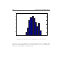
9.1 Rocket Dynamics . . . . . . . . . . . . . . . . . . . . . . . . . . . . . 61
9.2 Result From Simulation . . . . . . . . . . . . . . . . . . . . . . . . . 63
10 Conclusion and Further Work
65
10.1 Conclusions . . . . . . . . . . . . . . . . . . . . . . . . . . . . . . . . 65
10.2 Further Work . . . . . . . . . . . . . . . . . . . . . . . . . . . . . . . 66
Bibliography
67
A Quaternion
69
Appendix
69
x
Contents
B Coordinate Systems
71
B.1 Payload Fixt Coordinate System . . . . . . . . . . . . . . . . . . . . 71
B.2 Thruster Plane Coordinate System . . . . . . . . . . . . . . . . . . . 71
B.3 Launch Pad Coordinate System . . . . . . . . . . . . . . . . . . . . . 71
C User Manual
C.1 File Structure . . .
C.2 Input . . . . . . . .
C.3 Output . . . . . .
C.4 Program Execution
Index
.
.
.
.
.
.
.
.
.
.
.
.
.
.
.
.
.
.
.
.
.
.
.
.
.
.
.
.
.
.
.
.
.
.
.
.
.
.
.
.
.
.
.
.
.
.
.
.
.
.
.
.
.
.
.
.
.
.
.
.
.
.
.
.
.
.
.
.
.
.
.
.
.
.
.
.
.
.
.
.
.
.
.
.
.
.
.
.
.
.
.
.
.
.
.
.
.
.
.
.
.
.
.
.
.
.
.
.
.
.
.
.
73
73
73
74
75
77
Chapter 1
Introduction
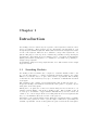
A sounding rocket is controlled by two separate control system for attitude control
and boost guidance. These system does not interchange any information, even
though they use similar subsystems. This result in an increased weight and volume
for the control system. Therefore is it desirable to merge these system into one
system. The purpose of the report is to examine the possibility to merge the impact
and attitude control functions for a sounding rocket to one system. Both hardware
(H/W) and software (S/W) have to be analyzed to determine the possibility to
design a merged system.
A preliminary design for a merged system is also done. The software for the design
is given in detail.
1.1
Sounding Rockets
A sounding rocket is a small rocket, compared to a satellite launcher, that boosts
up over the atmosphere to conduct experiments and then returns to the earth.
This is a cost effective way to do space related science experiments. The sounding
rocket flies in a suborbital trajectory up to an altitude of 200-700 km and then
down again.
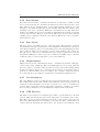
The sounding rocket consists of several subsystems, that are listed in table 1.1.
A typical sounding rocket mission is divided into three parts, boost phase, experiment phase and reentry phase.
During the boost phase the rocket is accelerates using the motors and the boost
guidance system (BGS) controls the sounding rocket. The sounding rocket is
boosted up to an altitude of approximative 100-700 km by the motor that can
consist of one or more stages. In the end of this phase the motors is separated and
the yo-yo mechanism reduces the roll rate of the payload.
An attitude control system (ACS) is used during the experiment phase to stabilize
and control the payload in order to give the right conditions for performing the
scientific experiments. In the reentry phase the payload reenters the atmosphere
1
2
Introduction
Table 1.1. Subsystems in a sounding rocket.
Subsystem
Motors
Function
Generates the thrust for the sounding rocket.
It can consist of one or more stages.
Payload
Experiments, control, recovery and service
systems.
Boost Guidance System
Controls the rocket during the boost phase.
The purpose of the system is to maintain
constant attitude and/or control the trajectory.
This is done in order to control the impact
point for the rocket. See section 1.2.
Attitude Control System
Controls the payload attitude during the
experiment phase. See section 1.3.
and deploys a parachute to soften the impact.
1.2
Boost Guidance System
The BGS controls the rocket during the boost phase. The purpose of the control is
to reduce the impact point dispersion for the rocket. The dispersion is minimized
to keep the impact point within the borders of the missile range. This is done by
controlling the trajectory and transverse attitude for the rocket.
The boost guidance is done during the duration of the motor burn.
There is mainly two means of controlling the rocket during the boost phase. Either
with canards or with thrust vector control. These methods are described in the
following sections.
The hardware for the BGS is listed in table 1.2.
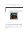
1.2.1
Actuators
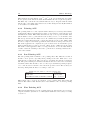
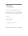
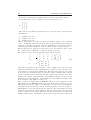
Aerodynamic control in the form of fins, so called canards, are used to control the
sounding rocket during the boost phase. A typical system that uses this strategy
is the Saab Ericsson Space AB (SE) DS19 seen in figure 1.1.
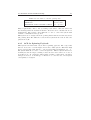
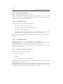
TVC controls the sounding rocket by altering the thrust vector of the motor. This
results in a change of the movement for the rocket. A system that uses this type
of control is the SE Guidance and Control System (GCS) seen in figure 1.2.
1.3 Attitude Control System
3
Table 1.2. BGS Hardware.
Components
IMS
Function
The Inertial Measurement System (IMS) is the sensor platform
the system. It usually contains gyros and accelerometers.
Computer
The computer is used for calculating the control strategies.
Actuator
The set of actuators are the part of the system that provides the
control forces on the body. This can be done with a servo system
with canards or with a thrust vector control (TVC) that is used
to control the direction of the motor thrust. See section 1.2.1.
Figure 1.1. The DS19 module
1.3
Attitude Control System
The ACS is used to control the sounding rocket during the experiment phase. The
main purpose for the control the payload during the experiments and reentry. The
control during the experiments are done of several purposes, they are for example,
minimize disturbances to achieve micro-gravity or control the pointing sequence to
perform observations.
This is done with rate and/or attitude control for the system. The ACS usually
uses a gas system as an actuator. A detailed description of the ACS can be found
in chapter 2.
4
Introduction
Figure 1.2. The GCS module
Chapter 2
Attitude Control System
In this chapter a more detailed description of the ACS will be presented including
a description of the parts in it.
2.1
Missions
The purpose of an ACS is to control the payload during the ballistic phase. The
control that is necessary is determined by the type of experiment that is conducted.
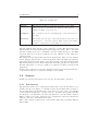
There is some basic kinds of missions listed in table 2.1. The share of each type of
missions compared to the total amount of sounding rocket missions flown by NASA
is also listed. The figures are derived from [13].
Mission type
Zero gravity
Solar
Coarse pointing
Fine pointing
Magnetic field
Non controlled
Table 2.1. Basic mission control.
Sensor
Rate gyro
Gyroplatform and sun sensor
Gyro platform
Gyro platform and star sensor
Magnetometers
No sensor
Accuracy
0.2◦ /s
1 arcsec
0.7◦
60 arcsec
2.0◦
-
%
10
10
30
20
5
25
Zero Gravity Missions
Experiments that require a zero-gravity environment is normally only controlled
in rate. The ACS used in this type of missions normally uses a gyro platform or
magnetometers to measure the rate. Descriptions of these sensors can be seen in
section 2.4.3 and section 2.4.4.
5
6
Attitude Control System
Solar Observation Missions
The sun is a target that often is studied during sounding rocket missions. Solar
observation missions have requirements on the attitude and rate of the payload for
the conduction of the experiments. These ACS uses sun sensors to determine the
direction towards the sun. Sun sensors is described in section 2.4.1.
Coarse Pointing Missions
This control is similar to the solar observation control. The differences are the
sensors used and the requirements on rate and attitude. The sensors used in these
missions are for instance gyros or magnetometers. A description of these can be
found in sections 2.4.3 and 2.4.4.
Fine Pointing Missions
The fine pointing control are similar to coarse pointing control but with higher requirements on accuracy for the attitude and rate. To achieve this a sensor platform
supported by a star sensor is used. The star sensor is described in section 2.4.2.
Magnetic Field Missions
The missions that are flown to conduct experiments on the earths magnetic field
usually use an ACS that uses magnetometers as sensors. These are described in
section 2.4.4.
Non Controlled Missions
There are some missions that do not need any kind of control during the ballistic
phase and no ACS is used at all.
2.2
ACS Hardware
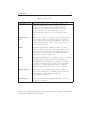
The components in the ACS are listed in table 2.2.
2.3
Actuators
An ACS normally uses a pressurized gas system as an actuator. The force acting
on the body is then generated when the gas is let out of nozzles.
The most commonly used system is the Cold Gas System (CGS). The CGS consists
of a pressure vessel containing the gas, regulators, nozzles and valves to control the
outlet of the gas. This system is based on a cold gas that generates the thrust.
There is also an other system, Hot Gas System (HGS). In this system the gas is
heated before it is used. The HGS consists of the same parts as the CGS and also a
device to heat the gas before it is let out the nozzles. More thrust can be generated
2.4 Sensors
7
Table 2.2. ACS Hardware.
Components
Sensors
Function
The system can have several sensors mounted on it. These
sensors are used to determine the attitude of the payload
during the flight. See section 2.4.
Computer
The computer is used for calculating the control strategies for
the ACS.
Actuators
The actuators is the part of the system that produces the force
that is used to control the payload. These actuators normally
consist of a gas system of some kind. See section 2.3.
this way with the same amount of gas compared to a CGS. The drawback for the
system is that the system itself has a higher weight and volume. Due to the small
amount of thrust needed for a sounding rocket the weight increase for the HGS
is greater then the decrease in weight for the gas. Therefore is the CGS most
commonly used.
The gas used in the CGS is nitrogen in most applications. There are also alternatives to this gas. Argon is also a commonly used gas. Argon and Nitrogen generates
approximately the the same thrust for the same amount of gas. The drawback with
Argon is that is has a lower outlet temperature then Nitrogen therefore larger nozzles and valves has to be used according to [4]. Therefore is Nitrogen used in this
application.
A CGS can be built in it is own self-contained module as long as it has an interface
to the main module for receiving and sending control signals.
2.4
Sensors
In this part various sensors that can be used by the ACS will be described.
2.4.1
Sun Sensors
The sun sensor is the most commonly used sensor type. It is used in almost every
satellite and also in a number of sounding rockets. For satellites this is because of
the fact that almost all satellites rely on the sun as a power source. In sounding
rocket applications this type of sensor is used to determine the attitude and also
the direction to the sun in the case where the sun is the object that will be studied.
This according to the sensor chapter in [16]. A drawback for the sensor is that the
attitude only can be determined in two axis.
There exist a variety of sun sensors on the market. They have somewhat different
functionality.
8
2.4.2
Attitude Control System
Star Sensors
Star sensors use the stars to determine the attitude. A star sensor consists of a star
detector and a star map. To determine the attitude the sensor takes a picture of the
stars. Then it tries to match the three to five brightest stars against an on board
star map, to determine in which direction it is facing. After this, the attitude of the
sounding rocket can be calculated. This sensor determines the absolute attitude in
all three axes unlike the previous. A drawback with this sensor is that it often has
a longer response time than the other sensors. The sensor is also heavier and has
a higher power consumption than the other sensors. This is also a more expensive
sensor then the other.
2.4.3
Rate Gyros
Gyros are used to determine the rate of the spacecraft. The principle of attitude
determination with gyros is integration of the angular rates measured by the gyros
and a known starting position. A benefit with gyros is the high sampling rate that
can be achieved. There are several types of gyros on the market, some of these are
listed in table 2.3. The most commonly used gyros in space applications today are
the FOG and DTG gyros. Silicon gyros are a relatively new kind of gyros. Because
of this they have not had enough time to prove their efficiency.
2.4.4
Magnetometer
Magnetometers use the earth magnetic field to determine the attitude. This type
of sensor have many advantages. They are small, light, have no moving parts and
they are tolerant to external conditions. However, there exist a disadvantage which
is that the magnetic field is not completely known and the models that exist for
prediction of the field have errors, according to [16]. Despite of this, the sensors
are commonly used, especially for experiments concerning the magnetic field.
2.4.5
Accelerometers
The only difference between commonly used accelerometers and the ones used in
spacecrafts is that the later has a smaller bias. This is because the spacecraft needs
extremely accurate information about the acceleration to be able to determine the
position. The accelerometer uses a mass that is attached to springs to determine
the acceleration. This is done by measuring the displacement of the mass.
2.4.6
GPS Receiver
The GPS receiver is used for low altitude spacecrafts to get information about their
position. This system is mostly used as an extra sensor for tracking of the rocket.
The GPS receiver provides information about the position and velocity for the
spacecraft. This information is normally not used by the ACS or BGS. But it is
common that the information is sent down to the ground control with the other
2.4 Sensors
9
Table 2.3. Rate Gyros.
Type
Mechanical gyro
Description
This is the standard type of gyros that consist of a
spinning disk that is mounted so that it can rotate
around one axis. The rate in the different axis is
measured by the deviation angel from the ground
position that the gyro gets. This type of gyro is
heavy and large. They are not as accurate as other
gyros.
Standard laser
gyro
These gyros consist of a platform where several mirrors
are mounted. The rate is measured by the interference
that occurs when the platform is spinning. These gyros
is fairly large and heavy. The accuracy is better then
for the mechanical gyro.
FOG
The Fiber Optical Gyro (FOG) is a laser gyro that
instead of mirrors uses fiber optics. This makes the gyro
both lighter and smaller then the standard laser gyro.
These gyros is both accurate and small which makes
them usable in space applications.
DTG
The Dynamically Tuned gyro (DTG) consist of a spinning
disk, that spins at a tuned frequency that makes it
dynamically decoupled from the sounding rocket. The
bending of the disk is then measured and compensated
for with a coil. This design makes the gyro efficient,
light and small. This gyro has a very god accuracy.
Wine glass gyro
These type of gyros vibrates and then the position of
the nodes is measured to determine the rate. This gyro
is extremely accurate but also sensitive to
environmental constrains.
Silicon gyros
These gyros are small and lightweight. They also have
a fairly good accuracy.
attitude and position information. The GPS receivers are normally used in pairs
to introduce redundancy in the system.
10
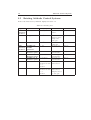
2.5
Attitude Control System
Existing Attitude Control Systems
A list of the ACS used by NASA is displayed in table 2.4.
Table 2.4. Existing ACS.
Type
Course
Attitude
Control
Fine
Attitude
Control
System
Rate Control
Accuracy
< 0.2◦ /s
Sensors
3-axis rate
sensor
Manufacturer
Space Vector
Magnetic ACS
< 2.0◦
Space Vector
Inertial ACS
< 2.0◦
MARK VIMARI
platform
MARK VIStellar Update
MARK VIStellar Pointer
MARK VI DStellar Update
SPARCS VI
< 3.0◦
Tree axis
magnetometer
single axis
rate gyro
MIDAS
platform
Inertial gyro
Inertial gyro
Star Tracker
Inertial gyro
Star Tracker
Inertial gyro
Star Tracker
Course/Fine
sun sensors
Aerojet
Course/Fine
sun sensors
Magnetometer
or rate gyro
NSROC
SPARCS VII
< 120 arcsec
< 60 arcsec
< 60 arcsec
< 1 arcsec
in Pitch & Yaw
< 5◦
in Roll
< 1 arcmin
in Pitch & Yaw
< 5◦
in Roll
Space Vector
Aerojet
Aerojet
Aerojet
NSROC
Chapter 3
Problem Formulation
This section contains an overview of how the control systems work today and the
purpose of the report. There will also be a description of the requirements on the
new system and how these are derived.
3.1
Purpose of the Report
The systems flown in present missions consist of two separate control systems for
attitude and trajectory control. These systems have no exchange of information
between them. Both of them use their own computer, actuators and sensor platform.
The purpose of this report is to study the feasibility of merging the two systems
into a single system.
3.2
DS19+
The system, called DS19+, that is designed is a combined ACS and BGS that uses
a DS19 module as the main structure. The DS19 module should be used with as
few changes as possible.
3.3
Requirements on the DS19+
The requirements on the system are that the boost control should remain the same
as for DS19. The requirements for DS19 can be found in [14].
The total pointing accuracy for DS19+ where no extra sensors are used should be
better than 0.7◦ , 3-σ. This requirement is derived from [3]. The first acquisition
maneuver, the maneuver to a new reference frame, should have a duration that is
less then 35 s.
11
12
Problem Formulation
The components in DS19+ shall follow the requirements on similar components in
DS19. If no mayor changes are done to the DS19 module these requirements will
automatically fulfilled. New components in DS19+ shall follow the requirements
in [3].
Chapter 4
DS19+ Heritage
This chapter discuss the use of present systems to design DS19+.
In the design of DS19+ knowhow and technical solutions from other SE control
systems is used, mostly from DS19 and RACS but also from SPINRAC these system
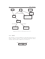
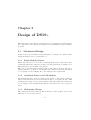
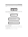
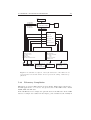
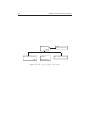
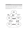
are described in section 4.1. The heritage tree for DS19+ can be seen in figure 4.1.
In section 4.2 the basic types of attitude control is described, the changes that are
needed in DS19 to achieve this functionality is also described.
4.1
Present Control Systems
These sections describe the systems that DS19+ is based on.
4.1.1
DS19
The DS19 system is a digital BGS. DS19 uses a gyro platform named DMARS as
a measurement instrument. The information from the gyro platform is computed
and a control signal is sent to the canards. This system can only function within
the atmosphere, because of the use of aerodynamic forces by the canards.
4.1.2
SPINRAC
SPINning Rocket Attitude Control system (SPINRAC) is a boost guidance system
that is used to minimize the impact dispersion by controlling the attitude of the
sounding rocket before the third stage of a large sounding rocket is ignited. This
is done with the use of an IMS controlled CGS system. A CGS is used instead of
canards because the control is done above the atmosphere.
13
14
DS19+ Heritage
DS19
RACS
SPINRACS
CGS
DS19
SPINRACS
MAGNETOMETER
DS19
RCS
DS19
ACS
(SPINNING PAYLOAD)
DS19
POINTING
STAR SENSOR
SUN SENSOR
DS19
SUN POINTING
DS19
FINE POINTING
Figure 4.1. Heritage tree with the DS19 module as base.
4.1.3
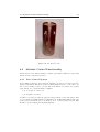
RACS
Rate and attitude control system (RACS) is a pointing ACS designed by SE, seen
in figure 4.2. RACS is constructed of a self contained module that uses a CGS as
an actuator. The performance of RACS can be seen in table 4.1.
Table 4.1. Performance for RACS.
Accuracy
Drift rate
±0.7◦
0.07◦ /s
4.2 Attitude Control Functionality
15
Figure 4.2. The RACS module
4.2
Attitude Control Functionality
In this section some functionalities for DS19+ and which additional components
that is needed for them is described.
4.2.1
Rate Control System
A free falling sounding rocket, with low angular body rates, provides a near zero
gravity environment. The Rate Control System (RCS) is used to control the body
rate of the sounding rocket to provide this environment. To achieve zero gravity
environment, two conditions must be fulfilled.
1. No acceleration of the body.
2. No angular body rates.
Condition one is met because the payload is in free fall above the atmosphere. The
second condition is fulfilled with a working RCS. A working RCS will hold the rate
of the payload less than 0.2◦ /s in all three axes. Control pulses from the RCS
should be avoided during the measurmentphase.
16
DS19+ Heritage
This results in an environment of 10−4 − 10−5 g. To get as much time as possible
in zero gravity environment the RCS shall minimize the rate as quick as possible.
The RCS only controls the rates which makes it easy to integrate with the DS19
system, since only additional S/W is needed. The changes in the H/W is limited
to an addition of a small CGS.
4.2.2
Pointing ACS
The pointing ACS is a control system with relatively low accuracy and stability
requirements. These requirements is possible to meet with no extra sensors beside
the IMS in the DS19. This makes the function easy to incorporate in DS19. The
system shall be able to point with an total accuracy of 0.7◦ , 3-σ in all three axis.
The incorporation with the DS19 is done in a similar way as with the RCS. The
difference is that this system also controls the attitude for the rocket. This results
in a more complex control strategy, with the effect that more CPU power is needed.
But as the application is computed in a period where there are much CPU power
unused, this should not cause a problem. There is also a difference in the CGS.
The CGS for this application has to be larger than the one for the RCS. This is
a result of that the sounding rocket has to perform more and larger maneuvers to
control the attitude.
4.2.3
Sun Pointing ACS
The sun pointing ACS is similar to the pointing ACS. The difference is that it
should be more precise, especially when pointing at the sun. This can be done
with the help of sun sensors. They are used to determine the attitude towards the
sun. The point of having several sensors is that the direction can be more accurately
determined. The ACS should be able to follow a predetermined pointing sequence
or be controlled via a real-time control from the ground control. The accuracy for
the sun pointing ACS should be according to table 4.2.
Table 4.2. Performance for the sun pointing ACS.
Accuracy
Drift rate
Resolution of the real-time control
±3.0 arcsec
2 arcsec/min
±(1 − 2) arcsec
This system can be seen as an extension of the pointing ACS with additional
sensors. The CGS for this ACS should be rater similar to the one in the pointing
ACS.
4.2.4
Fine Pointing ACS
This system shall function as the pointing ACS but with much better accuracy
compared with the systems above. This system shall have an accuracy according
to table 4.3.
4.2 Attitude Control Functionality
17
Table 4.3. Performance for the fine pointing ACS.
Accuracy
Drift rate
Resolution of the real-time control
±(2 − 5) arcmin
10 arcsec/min
±(1 − 2) arcsec
These requirements could be met by adding a star sensor. The star sensor has
the advantages that the attitude in all three directions can be calculated from one
measurement. The ground control shall also be able to control the system with
real-time commands from the ground.
This system can be designed from the pointing ACS in almost the same way as the
sun pointing ACS. The difference between these systems is the sensors and some
parts in the S/W.
4.2.5
ACS for Spinning Payloads
This system is an ACS thats only works for spinning payloads. The components
that are needed are a 3-axis magnetometer and a CGS system. This ACS shall
hold a payload that spins with 0.5 − 2.0 rps and within an alignment of 1 − 2◦ .
The system shall also be able to control the spin rate. This is a system that is not
normally used in the larger sounding rockets, therefore there will be no focus on
it in this report. To expand the functionality of DS19 to this system only minor
changes are needed. So if this type of ACS were to come into use, a new system
could quickly be designed.
18
DS19+ Heritage
Chapter 5
Design of DS19+
The integration between the two systems can be done in many ways. In this chapter
the components of the systems are analyzed and a preliminary design for DS19+
is derived.
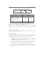
5.1
Mechanical Design
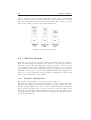
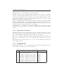
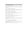
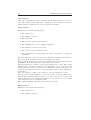
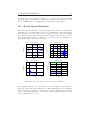
In this section the mechanical design alternatives of DS19+ are described The
design alternatives can be seen in figure 5.1.
5.1.1
Single Module System
This solution is based on one module containing all the parts of the system. The
benefit with this is the reductions of joints between modules in the sounding rocket.
This will increase the strength of the system.
There are some drawbacks with this solution. The first is the large amount of
changes that has to be made to the DS19 module. Another is that the system has
to be redesigned between flights due to the changes in the requirements.
5.1.2
Combined Sensor and CGS Module
The structural changes from the single module design to this design is that the
sensors and CGS is moved from the DS19 module to a separate module. This
design has the benefit of a more intact DS19 module. The drawbacks is that it has
to be redesigned between missions and that the extra sensors not can be positioned
freely.
5.1.3
Modularized Design
This design has an intact DS19 module and has two extra modules. One for the
CGS and one for the extra sensors.
19
20
Design of DS19+
The two separate modules for sensors and CGS is chosen because in most flights
the sensor module is not needed and can then be easily excluded. The structure
also gives extra freedom for the position of the sensors. The construction of the
CGS can also easily be made by an external manufacturer.
Figure 5.1. The design alternatives.
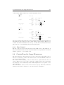
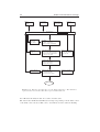
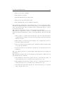
5.2
Cold Gas System
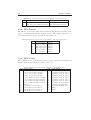
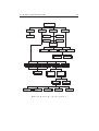
The CGS for the payload is chosen to have the schematic design according to
figure 5.2. The regulators and latching valve is used to control the gas pressure by
the solenoid valves. The roll thrusters are activated in pairs to reduce the effect
on the transverse axes. The configuration makes it possible to use two pressure
levels. This is necessary because then large errors can be quickly corrected and the
minimum error that can be corrected is still sufficiently small. The minimum error
that can be corrected depends on the gas pressure, minimum active time for the
solenoid valves and the size of the nozzles.
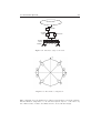
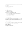
5.2.1
Thruster Configuration
The position of the thrusters are chosen according to figure 5.3.
The thruster position is chosen in straight angles to be able to control all possible
transverse axes. This is the best choice if the direction of the thrusters not can be
changed during the flight. The position of the roll thrusters, that are the thrusters
that is position in pairs by the x axis, are chosen to reduce the effect on the
transverse axes from them. The roll thrusters are only operated in pairs to get a
clean roll maneuver. These thruster is not necessary placed in the same plane as
the transverse thrusters.
5.2 Cold Gas System
21
PRESSURE VESSEL
REGULATOR 1
LATCHING
VALVE
REGULATOR 2
SOLENOID
VALVES
NOZZLES
Figure 5.2. Schematic design of the CGS.
Figure 5.3. The thruster configuration.
This configuration for the thrusters are valid for systems that controls the attitude.
Another thruster design has to be chosen if the system only is to control the body
rate. This because of that some thrusters is not needed in that design.
22
5.3
Design of DS19+
Budgets
This section contains the mass, gas and power budget for DS19+.
5.3.1
Mass Budget
The changes in the weight is some loss in the weight due to the synergism effect
that occur when the systems is merged, such as the removal of similar components
used in both systems, for example IMS and battery.
There is two benefits that can occur when the weight is lowered for the sounding
rocket either can the weight of the payload be increased, which gives room for more
experiments or the maximum apogee is increased, which results in a increase of the
time for the experiment phase of the flight.
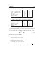
5.3.2
Gas Budget
In this section the gas consumption for DS19+ is discussed.
To estimate the amount of gas needed in the CGS system, data from typical sounding rockets are used, see table 5.1. This table shows the moment of inertia and
other physical properties two sounding rockets.
Table 5.1. Rocket Properties for Sounding Rockets.
Moment of Inertia, Roll (kg m2 )
Moment of Inertia, Pitch/Yaw (kg m2 )
Lever, Roll (m)
Lever, Pitch/Yaw (m)
Small
10
1000
0.22
1.3
Large
23
2700
0.22
2
The gas consumption for the RACS sounding rocket can be found in [7], this
consumption is listed in table 5.3 and the physical properties for the rocket is
listed in table 5.2.
Table 5.2. Physical Properties for RACS.
Moment of Inertia, Roll (kg m2 )
Moment of Inertia, Pitch/Yaw (kg m2 )
Lever, Roll (m)
Lever, Pitch/Yaw (m)
10
500
0.22
1.000
The acquisition maneuver consists of several phases. One roll rate reduction from
90◦ /s to 0◦ /s and one transverse rate reduction from 25.7◦ /s to 0◦ /s and also one
180◦ transverse reorientation maneuver.
The RACS ACS is a system that can perform a large amount of maneuvers. Most
of the reorientation maneuvers is not necessary in other ACS. The gas that is used
by RACS for a nominal ACS mission is according to table 5.4.
5.3 Budgets
23
Table 5.3. Amount of Gas needed for RACS.
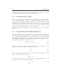
Maneuver description
Acquisition maneuver
5 ∗ 30◦ (0◦ off thruster axis)
2 ∗ 40◦ (45◦ off thruster axis)
10 ∗ 45◦ roll
180◦ transverse reentry maneuver
Spin-up before reentry
Duty-cycle pulsing
Dumping
Total impulse
Impulse [Ns]
614
515
187
290
220
80
60
15
1981
Gas Mass [kg]
0.97
0.82
0.30
0.46
0.35
0.13
0.1
0.02
3.15
Table 5.4. Amount of Gas needed for RACS in nominal flight.
Maneuver description
Acquisition maneuver
Maneuvers during flight
180◦ transverse reentry maneuver
Spin-up before reentry
Duty-cycle pulsing
Dumping
Total impulse
Impulse [Ns]
614
300
220
80
60
15
1289
Gas Mass [kg]
0.97
0.5
0.35
0.13
0.1
0.02
2.07
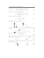
From this information the amount of gas that the typical sounding rockets use are
derived, by looking on how the moment of inertia and the levels, i.e the distances
between the center of mass and the nozzle, have changed. The impulse amount
needed for a maneuver that uses an impulse of M2 for another rocket becomes:
M1 =
I1 R2
M2
I2 R1
(5.1)
Where the values represent the following:
• M1 is the moment needed for rocket one.
• M2 is the moment needed for rocket two.
• I1 is the moment of inertia for rocket one.
• I2 is the moment of inertia for rocket two.
• R1 is the length of the level for rocket one.
• R2 is the length of the level for rocket two.
M1
The results from these calculations are shown in table 5.5 where the terms M
are
2
shown for each axis for the rockets. Where M2 is the moment needed for RACS.
24
Design of DS19+
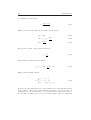
Table 5.5. Scaling factors for gas consumption.
In Roll
In Pitch and Yaw
M1
Small ( M
)
2
1
1.54
1
Large ( M
M2 )
2.3
2.7
Table 5.6. Amount of gas needed for the standard rockets.
Maneuver description
Acquisition maneuver
Maneuvers during flight
180◦ transverse reentry maneuver
Spin-up before reentry
Duty-cycle pulsing
Dumping
Total impulse
Small (17 in) Large (22 in)
Impulse [Ns]
891.6
1617.8
408
770
339
594
80
184
90
162
20
20
1828.6
3347.8
Table 5.4 are used as a base for the making of table 5.6 which shows the gas
consumption for a nominal flight with the standard rockets.
As shown in table 5.6 the amount of gas needed for the rockets are very shifting
between the rockets. Therefore the best design is to have the CGS in a separate
module.
5.3.3
Power Budget
This budget is done in order to investigate if the battery in DS19 has enough power
to support the complete DS19+ system.
Power Consumption
The parts that consume energy in the system are the DMARS, which is the internal
measurement unit (IMU) in DS19, power distributing unit (PDU), attitude sensors,
the pressure sensors, the CGS and the servo system for the canards.
• The DMARS has a consumption of 1 A in the nominal case according to [11]
and a flight does nor last for more than 30 min. The power consumption of
the DMARS is according to these numbers 0.5 Ah.
• The PDU in the RACS system has a power consumption of 0.055 Ah according to [15]. The PDU in the DS19 has a similar structure as this one. A
restrictive number on the power consumption is then 0.1 Ah.
• To get a restrictive power consumption for the extra sensors, several sensors
are studied. The highest power consumption for the sensors where found to
be 0.4 Ah.
5.4 Electrical Interfaces
25
• The power consumption of all three pressure sensors is set to 0.25 Ah. This
number is derived from the fact that one old pressure sensor from the RACS
consumes 0.055 Ah according to [15].
• To empty the CGS completely in the RACS 0.113 Ah is needed according
to [4]. The CGS for this application is up to 1.7 times as large as the RACS
system. Therefore a consumption of 0.2 Ah is a restrictive number on the
consumption.
• The power consumption that is needed for the canard servos is also derived
from the RACS CGS power consumption. This because of that the servo
system works in a similar way as the CGS. The servo system is naturally
much smaller and therefore easier to empty. A restrictive number for the
power consumption for the servo system are 0.1 Ah.
The results of the power consumption will be according to table 5.7.
Table 5.7. Power consumption.
Activity
Pressure sensors
DMARS
PDU
CGS
Servo system
Attitude sensors
total
Consumption [Ah]
0.25
0.5
0.1
0.2
0.1
0.4
1.55
Conclusions
From table 5.7 the worst case power consumption is 1.55 Ah and according to [1]
the power that can be generated from the battery in the DS19 is 2.2 Ah. This
gives a resulting over capacity of 42%. For the ACS were no extra sensors is used
the power consumption is as low as 1.15 Ah which result in a over capacity of 91%.
The power consumption is calculated with a run time of 30min, which is longer
then any run time for the system.
This gives the result that the battery power is sufficient to support the complete
system. If this had not been the case the battery system would have been extended
with either a new sort of batteries in the DS19 module or extra batteries in the
DS19 or CGS module.
5.4
Electrical Interfaces
The merging of the system results in several new interfaces that has to be added in
the DS19 module. These interfaces emerge because new signals are needed in the
system. These signals result in the new or changes interfaces listed in table 5.8.
26
Design of DS19+
There is also some extra data that has to be sent by the telemetry from the DS19
to the ground. This will only cause some minor changes in the telemerty (TM)
format.
Table 5.8. New or changed interfaces.
From
DMARS
PDU
PDU
To
PDU
CGS
Extra Sensors
The extra data that need to be sent between the DMARS and the PDU is listed
in table 5.9. In the same way the new signals for PDU to CGS and PDU to Extra
Sensors is listed in tables 5.10 and 5.11.
Table 5.9. New signals between PDU and DMARS.
Control signals for the CGS.
Data from the CGS.
Control signals for the sensors.
Data from the sensors.
Table 5.10. New signals between PDU and CGS.
Control signals for the solenoid valves.
Control signals for the latching valve.
Measured pressures from the CGS.
Power supply and ground connection to the CGS.
Table 5.11. New signals between PDU and Attitude Sensors.
Control signals to the sensor.
Data from the sensor.
Power supply and ground connection to the sensor.
5.4.1
Design Options
There are several designs for the electric interfaces between DMARS and PDU.
Three alternative designs are:
Reassociation: Remove signals from the present interface to create room for new
important signals.
Rebuilding: Rebuild all the interfaces to fit in all signals.
5.4 Electrical Interfaces
27
Sharing: Share the existing pins between the signals.
The first design is easy to implement and results in minor changes to the DS19
module. The drawback with this design is that it does not free enough space
for the sun pointing ACS, the real-time control and the RCS, this due to that
a interface towards the payload is needed during this control to stop the control
pulsing during sensitive measuring phases.
The second design gives the best interfaces but also the largest changes in the DS19
module. This design is the best one if further changes has to be done in the system.
The third solution is time demanding and difficult to implement and it does not
solve any problem better then any of the other designs.
The PDU has to be rebuild for all solutions. This because an interface towards
the CGS is needed and there are no space for this interface in the present design,
see [10].
5.4.2
Implemented Design
The design that is chosen for implementation is the design that is based on reassociation of the pins. It is chosen based on that it is easy to implement and that
there exist signals that currently are unused that can be removed.
The choice of design results in that the sun pointing ACS, RCS and real-time can
not be done. Therefore is these control systems excluded from the rest of the
report.
The changes in the interfaces needed to be done for this design are described in
the following sections.
5.4.3
DMARS-PDU
The changes that has to be done in this interface for the chosen design is reassociation of pins according to table 5.12 and table 5.13.
Table 5.12. Pin reassociation in 44 pins DMARS to PDU interface.
pin
22
23
33
34
35
36
37
38
39
New signal
CGS bottle pressure
CGS regulated pressure
Opening command solenoid
Opening command solenoid
Opening command solenoid
Opening command solenoid
Opening command solenoid
Opening command solenoid
Opening command latching
valve
valve
valve
valve
valve
valve
valve
1
2
3
4
5
6
Old function
IMS temperature
Deck temperature
Empty
Empty
Empty
Empty
Empty
Empty
Empty
28
Design of DS19+
Table 5.13. Pin reassociation in 26 pins DMARS to PDU interface.
pin
22
23
5.4.4
New signal
TX extra sensor RS232 interface
RX extra sensor RS232 interface
Old function
TX GPS RS232 interface
RX GPS RS232 interface
PDU-Sensors
The interface between the PDU and the arm-safe plug has free pins that can be
used for communication with the attitude sensors. The changes that has to be
done in this interface are the ones described in table 5.14.
Table 5.14. Pin reassociation in 25 pins PDU to arm-safe plug interface.
pin
6
7
12
13
22
23
5.4.5
New signal
Power feeding
Power feeding
TX extra sensor
RX extra sensor
Power ground
Power ground
Old function
Empty
Empty
Empty
Empty
Empty
Empty
PDU-Valves
The communication between the PDU and the valves could be done through a new
interface with pin association according to table 5.15.
Table 5.15. Pin association in 25 pins PDU to VALVES interface.
pin
1
2
3
4
5
6
7
8
9
10
11
12
13
New signal
+5V bottle pressure measure
-5V bottle pressure measure
Out bottle pressure measure
Out bottle pressure measure
+5V regulated pressure measure
-5V regulated pressure measure
Out regulated pressure measure
Out regulated pressure measure
Empty
Operating solenoid valve 1
Operating solenoid valve 1
Operating solenoid valve 2
Operating solenoid valve 2
pin
14
15
16
17
18
19
20
21
22
23
24
25
New signal
Operating solenoid valve
Operating solenoid valve
Operating solenoid valve
Operating solenoid valve
Operating solenoid valve
Operating solenoid valve
Operating solenoid valve
Operating solenoid valve
Operating latching valve
Operating latching valve
Empty
Empty
3
3
4
4
5
5
6
6
5.4 Electrical Interfaces
5.4.6
29
Changes in the TM format
The change that has to be done in the TM format are that other data has to be
sent to ground control depending on which control function that is active.
The changes that has to be done are the following:
• If the BGS control is active changes in the TM format according to table 5.16
has to be done.
• If the ACS control is active changes in the TM format according to table 5.17
has to be done.
Table 5.16. Changes in the TM during BGS control.
New Data
Old Data
For the 100 Hz data
No changes
For the 20 Hz data
Information on which control that is active. Empty
For the 4 Hz data
The bottle pressure for the CGS.
Temperature DS19 structure
The regulated pressure for the CGS.
Temperature DS19 gyro
The starting time for the ACS control.
Empty
The lowest starting altitude for the ACS
Empty
control.
Table 5.17. Changes in the TM during ACS control.
New Data
Old Data
For the 100 Hz data
The command word to the CGS valves.
Reference attitude in pitch.
The regulated pressure for the CGS.
Reference attitude in yaw.
For the 20 Hz data
Information on which control that is active. Empty
Reference quaternion 1.
Command signal pitch canards.
Reference quaternion 2.
Command signal yaw canards.
Reference quaternion 3.
Return signal from pitch servo.
Reference quaternion 4.
Return signal from yaw servo.
For the 4 Hz data
The bottle pressure for the CGS.
Temperature DS19 structure
The regulated pressure for the CGS.
Temperature DS19 gyro
The starting time for the ACS control.
Empty
The lowest starting altitude for the ACS
Empty
control.
30
5.5
Design of DS19+
Software Expansion for DS19+
The changes that are needed in the S/W for the combined system is addition of
new control strategies for the ACS control. Mainly how the CGS will be controlled
based on the present attitude and rate. This results in a control routine that has to
be computed during the ballistic phase of the flight. This control routine is never
done at the same time as the control routine for the boost guidance. Therefore is
the CPU power in the present system enough for both applications. The only other
thing that needs to be computed during the time the strategies are computed is
the TM signal. This is already done in the present system so the difference should
not be significant.
5.5.1
Existing Software
The code that is used as a ground for the DS19+ S/W is the flight S/W from
the DS19 module. This S/W is flight proved and many of the functions that are
used in it can be used in the ACS S/W without any modification or very small
modifications.
The largest changes that are needed to be done are the functions that are used for
the attitude control computation. This includes an attitude reference computation
and the function that computes the control law.
5.5.2
New Functionality
There are two completely new functions that have to be implemented in the DS19+
for the ACS control.
ACS Control Function
The first one is a function that computes the control law for the ACS. This function
uses a completely different strategy compared to the DS19 control algorithm. This
is due to the use of other actuators and also the fact that the ACS controls the
rocket in all three axis and the DS19 only controls it in two axis. For the ACS that
uses extra sensors this function needs to consider the sensor information as well as
the gyro information.
This function uses information from the IMS and the reference attitude as input
for the ACS that does not use extra sensors. From this information the control
signals to the valves is computed. This signal is then the output from the function.
The function uses the control laws described in chapter 6.
ACS Reference Computation
The second is a function that takes the time as input and returns the reference
and reentry flag as output. The attitude reference is given in quaternions, the
quaternions are described in appendix A. The function is the same for all ACS
that has a requirement on the reference attitude.
5.6 Conclusions
31
The function matches the time to the index in a table. If there is a new attitude
there will be a transition phase that uses linear interpolation between the present
and new attitude.
This function is not the same as the reference computation for the BGS because
the ACS needs a fix reference in all three axis. The BGS uses a reference that is
calculated from a formula that only returns a reference in pitch and yaw.
5.5.3
Design Considerations
The changes that has to be done in the other functions is that in all communication
functions ACS commands has to be added. A changing command between BGS
and ACS also has to be added, to determine which of the attitude control laws
and reference computation that is to be used. This criteria is used in the top level
control.
A study of the feasibility of the combination of the code has also been done. From
this study the results are that there is enough computation power and memory
capacity in DS19 to handle both a BGS and a pointing ACS.
5.6
Conclusions
The design that is chosen for the system is specified in this section.
The design that is chosen is a modularized design for the structure of the system,
this is done to get a flexible system that has a minimum of changes in the DS19
module. The budgets that is done indicates that the power supply from DS19 is
enough to support the complete system. Therefore is there no need to include extra
batteries in DS19+. The budget for the gas is done in order to know how large the
CGS has to be for a specific sounding rocket.
The chosen design for for the electrical interfaces in the system is based on reassociation of pins to make room for the new data. The reassociation is done
according to section 5.4.2. The changes in the TM format also has to be done for
this application. This design does only free enough space for the pointing ACS.
If any other attitude control application is done a redesign for the IMS and specially the interfaces is recommended. The changes in the TM format also has to
be redesigned.
The software design is therefore done for a DS19+ with a pointing ACS. The
computer and memory capacity in DS19 is enough for this system.
32
Design of DS19+
Chapter 6
Control Law
In this chapter the control law concept that is used for the ACS and RCS is discussed.
6.1
Control Concepts
Several concepts can be considered for use in both the ACS and RCS control. The
report will focus on Bang-Bang control for the control system. This is because
the thrusters only has two states, open or closed. There are two forms of control
strategies that can be implemented, both of these use Bang-Bang control. The
first one is a minimization of a loss function. The other one is the use of fuzzy
control. The first strategy gives more calculations for the flight computer but has
the advantages that already flight proved code can be used for the implementation,
therefore that strategy is chosen.
There are two sorts of Bang-Bang control with loss functions that can be implemented.
The first one is the Bang-Bang control for 3-dimensional control, where the complete control is computed from one algorithm. This algorithm uses the attitude
error in all axes and also the angular velocity in all axes. This results in an algorithm that is very precise. A drawback with this is that it is very complex to do
and results in difficult calculations and optimization problems.
The other alternative is to handle each axis separately and then combine them into
one control algorithm. This is somewhat less optimized for the whole problem.
But the computations is much easier and faster. There is some loss in the solution
due to that the problem only is optimized for the different axes and not the whole
problem.
For the ACS, a combination of these methods is used. The control is constructed
that way to optimize the control for the cases in the flight.
For the RCS, the Bang-Bang control is also chosen but the switching lines is only
depending on the body rate of the rocket. Therefore the switching criteria will be
33
34
Control Law
straight lines in the plane. In this case the 3-axis problem is divided into 3 1-axis
problem. This simplifies the solution and implementation.
6.2
Control Law for ACS
There are some differences between the control for small and large maneuvers. The
largest different is that the error has to be sufficiently small for small maneuvers
so that only local optimum switching criteria have to be studied and not global
optimum switching criteria as in large control. Due to this the control law for small
maneuvers can be divided into three separate control laws, one for each axis. The
control law for large maneuvers has to have one control law for the whole system
except the roll axis which is possible to control separately.
Therefore are the control functions for the large and small control are studied
separately.
6.3
Control Law for Small Maneuvers
The control law that is chosen for this case is a one axis loss function. This control
law will result in a switching criteria for the thrusters that are lines in the phase
plane. This plane has the angular velocity and the attitude error as axis. The lines
are derived from the solution to an optimization problem. The solution is obtained
by minimizing the Hamilton function H. These computations are similar to those
in [6]. These calculations are similar for all axes.
min H = L + Vϕ ϕ̇ + Vω ω̇
(6.1)
(6.2)
Where ϕ is the attitude error, ω the angular velocity and Vϕ and Vω are loss
functions. The following relation holds for the derivate:
ϕ̇ = ω
ω̇ = au
(6.3)
(6.4)
Where a is the angular acceleration produced by the thrusters and u is the control
signal. u has the following properties:
u ∈ {0, 1, −1}
L is a function of λ and u. λ is a design parameter that represents the trade off
between gas consumption and maneuver time.
L = 1 + λ|u|
λ≥0
(6.5)
6.3 Control Law for Small Maneuvers
35
The function that is going to be minimized then gets the form:
min H = 1 + λ|u| + Vϕ ω + Vω au
u
This results in three cases for the minimization:
,u = 0
1 + Vϕ ω
min H = 1 + λ + Vϕ ω + Vω a , u = 1
u
1 + λ + Vϕ ω − Vω a , u = −1
These equations gives the following result:
, −λ > Vω a
1
u = −1 , λ < Vω a
0
, −λ ≤ Vω a ≤ λ
(6.6)
(6.7)
(6.8)
The equations for motion from Hamilton is:
∂H
= ϕ̇ = ω
∂Vϕ
∂H
= ω̇ = au
∂Vω
∂H
= −V̇ϕ
∂ϕ
∂H
= −V̇ω
∂ω
∂H
dL
=
∂t
dt
H = L + Vϕ ϕ̇ + Vω ω̇
In combination with the results from above and these equations the following result
is derived.
∂H
= 0 ⇒ Vϕ = C
(6.9)
∂ϕ
∂H
= Vϕ ⇒ V̇ω = −Vϕ = −C ⇒ Vω = −Ct + D
∂ω
The steady state solution for the Hamilton function is:
min H = 0
(6.10)
(6.11)
u
This result must also be valid for u = 0 therefore must C = − ω1 . The switching
lines can be derived from equation 6.8.
λ = Vω a
λ = −Vω a
(ON )
(OF F )
(6.12)
(6.13)
These criterias can be rewritten with the values from above. Where t1 and t2 is on
and off times for the control.
t1
(ON )
λ = a( + D)
(6.14)
ω
t2
(6.15)
λ = −a( + D)
(OF F )
ω
36
Control Law
A combination of these gives:
λ=
a(t1 − t2 )
2ω
(6.16)
This gives the following change in the attitude for the system.
∆ϕ = ϕ̇∆t
(6.17)
∆t = t1 − t2 =
2ωλ
a
(6.18)
2
∆ϕ =
2ω λ
a
(6.19)
The criteria to switch on the system is then set to:
ϕ1 =
ω2
2a
(6.20)
This results in a switch off criteria that is:
ω2
(1 + 4λ)
2a
(6.21)
; ϕ < −ϕ2
a
U = −a ; ϕ > −ϕ1
0
; −ϕ2 ≤ ϕ ≤ −ϕ1
(6.22)
ϕ2 = ϕ1 + ∆ϕ =
This gives the switching criteria:
To reduce the duty pulsing that can occur for small errors a dead band is introduced
in the equation. The dead band is symmetrical around zero and it is δ wide. A
reducing factor, ρ, is also introduced. ρ is a reduction factor that is introduced to
avoid overshoots. This is done because of the large negative effect an overshot has
6.4 Control Law for Large Maneuvers
37
on the system. This results in the modified switching criteria.
ω>0:
ϕ>δ:
ϕ<δ:
−δ ≤ ϕ ≤ δ :
ω<0:
ϕ < −δ :
ϕ>δ:
−δ ≤ ϕ ≤ δ :
U = −a
a
U = −a
0
−a
U=
0
; ϕ < −ϕ2 − δ
; ϕ > − ϕρ1
; −ϕ2 − δ ≤ ϕ ≤ − ϕρ1
q
2δ
; ϕ > −ω aρ
+δ
q
2δ
; ϕ ≤ −ω aρ
+δ
U =a
; ϕ < ϕρ1
a
U = −a ; ϕ > ϕ2 + δ
0
; ϕρ1 ≤ ϕ ≤ ϕ2 + δ
q
a ; ϕ < −ω 2δ − δ
q aρ
U=
0 ; ϕ ≥ −ω 2δ + δ
aρ
(6.23)
One more variable that is introduced in the switch criteria is a hysteresis function
that make the system hold a specific output during a time interval. This is done
to make sure that the thrusters does not go on and off every interval, when the
system is close to the switching criteria in the phase plane.
6.3.1
Fine Control
The fine control is done in the same way as the small control. The difference is
that other numbers is used for the criteria and that a lower pressure is used which
makes it possible to correct small errors.
6.4
Control Law for Large Maneuvers
The large maneuver control law is based on the control law for the RACS control,
that can be found in [5]. This control law is based on the same Hamilton function
as for the small maneuvers.
The control of the sounding rocket is divided in two parts transverse and roll
control. This can be done because of that the coupling between the roll axis and
the transverse axes is sufficiently small. This simplifies the development of the
control system.
The control that is derived for the control is based on (6.22). Where the transverse
maneuver is the main contributor to the time and fuel consumption.
38
6.4.1
Control Law
Roll Control
The roll control is divided into two separate procedures.
Rate reduction: This procedure reduces the roll rate before the the attitude
control starts.
Attitude control: In this procedures the roll attitude is controlled. The control
algorithm that is used are similar to the attitude control for small maneuvers 6.23.
6.4.2
Transverse Control
The transverse control will be designed as if the thrusters can be used in an arbitrary direction in the transverse plane. This is not true because the thrusters
is mounted with a straight angle between them. This approach is however valid
because the real problem is solved by ξL where L is the idealized loss function and
ξ is the factor:
√
1 + 2λ
ξ=
1+λ
This is done because the thrust is in fix directions and not in arbitrary directions
as the loss function is calculated for, this according to [5]. The control strategy is
based on several locally optimal trajectories. The the most optimal is chosen from
loss functions for the system. The local trajectories are based on the trajectories
from RACS ACS, described in [5].
These trajectories describe solution of how the payload can go from the present
state to the wanted state. A loss function is calculated for each trajectory and
then the smallest of them is chosen as base for the control. The choice between the
trajectories are done for every call to the large control.
The trajectories are:
L1 This loss function represent a trajectory that is made of one turn towards the
reference attitude, a coast phase and a deceleration phase.
L2 This loss function represent a trajectory that consists of a deceleration to a
complete halt followed by a attitude maneuver in one axis.
L3 This loss function represent a trajectory that consists of a coast phase followed
by a deceleration and finally a maneuver in one axis.
L4 This loss function has a trajectory made of a coast phase followed by a combined
turn and deceleration. This function is valid for small equatorial rates.
L5 This function has a trajectory made of an acceleration towards the reference
attitude. This function is valid for small equatorial rates.
6.5 Control Law for RCS
39
L4 and L5 is needed because the others has discontinuities for small equatorial
rates. The drawback with them is that they are only valid for a restricted domain.
The loss functions are only valid for specific intervals. If the state of the sounding
rocket is outside the valid interval the loss function is set to infinity. At least one
function is always valid.
6.5
Control Law for RCS
The Control law used in the RCS is the same as the one used for rate reduction
in the ACS. This control is also based on Bang-Bang control and uses a Hamilton
function similar to the Hamilton function in the attitude control. The loss function
for the rate control has the following form:
s
2
Cx ωx 2 C⊥
L= (
) + 2 (ωy2 + ωx2 )
ax
a⊥
Where a is the angular acceleration and C is a weight constant for each axis. The
loss function inserted in the Hamiltonian then results in a control law with the
following form:
; ω ≤ −f (a, C, λ, L)
a
u = −a ; ω ≥ f (a, C, λ, L)
0
; −f (a, C, λ, L) < ω < f (a, C, λ, L)
Where f (a, C, λ, L) is a function determined by the minimization of the Hamilton
function. This is the principle for both large and small angular rates. The difference
between them is the constants. The switching between them is based on a similar
logic as the switching between the attitude control functions.
40
Control Law
Chapter 7
Architectural Software
Design
The S/W for the system is divided in two subsystems.
• The S/W for the IMS.
• The S/W for the Guidance and control (G&C) application.
The S/W for subsystem one is designed and written by the developer of the IMS.
This design is therefore not considered in the rest of the report. Instead the architectural design of the G&C application will be discussed. The architectural design
for the top level of DS19+ is mainly the same as for the DS19. Therefore much of
the architectural design is derived from [9].
7.1
System Design
The main functions of the G&C application are listed in table 7.1. The design is
focused on the functions and changes that are generated from the adding of the
ACS functionality to the system. The final program shall be written in C to be
compatible with the existing code.
Table 7.1. Purpose of the G&C application S/W.
Impact point calculations.
Parameter scheduling.
Telemetry compilation.
Command calculations for:
Attitude control calculations for:
41
Canards
Thruster valves
BGS application
ACS application
42
Architectural Software Design
7.2
Interfaces
The interfaces can be divided into three parts:
• All S/W interfaces between IMS and G&C.
• The signals from the G&C application to the digital output and to the digital
to analog converter (DAC).
• All other S/W to H/W communication.
The design only handles the first two parts listed above. The third part is handled
by the IMS S/W.
The interfaces between the different S/W applications are handled by a header file.
This file shall be included in both IMS and G&C application files. The interchange
of data is partly done through partly pointer references in the program and by
global data. All signals to or from the H/W that not is handled by the G&C
application is routed through the S/W of the IMS.
A schematic description of the system is seen in figure 7.1.
7.3
Initialization
The initialization is handled by a function that is called by the IMS at startup
for the system. The function sets all variables and parameters that has to be
predefined. The function is divided into subfunctions for the different subsystems
of the S/W.
7.4
Guidance and Control Calculations
This section contains a short description of the functions in the G&C application.
A description of functions and data flow for the G&C application can be seen in
figure 7.2.
7.4.1
Parameter Scheduler
This function selects predefined parameters from tables using the time since lift-off,
velocity, attitude and position parameters. The function then interpolates a value
from the table which is returned to the program. The values that can be stored in
the table is for instance parameters for the BGS control.
7.4.2
Impact Point Calculations
This function takes IMS data as input and calculates the apogee altitude, time to
impact, impact point and the corrections of the attitude reference. This information
is then returned to the main function.
7.4 Guidance and Control Calculations
43
G&C
INITIALIZATION
TM BUFFER
INTERRUPT
INTERRUPT HANDLING
SENSOR
DATA
IMS APPLICATION
EGSE CMD
SPORADIC
INTERRUPT
100Hz INTERRUPT
USER.h
SEND TM
SEND EGSE
SENT IMS CMD
IMS DATA
ANALOG DATA
IMS APPLICATION
G&C APPLICATION
COMMUNICATION
TM, EGSE OUTPUT
START−UPP
CALIBRATION
SAMPLING ANALOG DATA
DECODE EGSE
ATTITUDE CONTROL
BGS
ACS
OUT DAC, DIGITAL
COMPILE TM
TM
SERVO
FOR CANARDS
EGSE
HWIL
PRESSURE FROM CGS
VOLTAGES
SERVO RETURN
LIFT−OFF DETECTION
CANARD DECOUPLING
READY−TO−LAUNCH
CGS VALVES
Figure 7.1. Schematic description of the S/W architecture. The thiner arrows
represent data flows and the thicker arrows represent the calling of different applications.
7.4.3
Telemetry Compilation
This function creates a TM format from given inputs. This format is then sent to
the IMS application to be routed to the ground control. The TM format contains
100Hz, 20Hz and 4Hz data.
In the 100 Hz data is for example the quaternions from the IMS sent. In the 20 Hz
data is for example the results from the impact point calculations sent. Finally in
44
Architectural Software Design
INPUT:
EGSE, IMS
ATTREF
DATA FROM:
IMS S/W
DIRECT OUT:
DAC
DIGITAL OUT
OUTPUT:
EGSE
TM
HEADER FILE
EGSE COMMAND
IMS MODE
G&C MODE
DECODE:
IMS DATA
ATTITUDE REF
ACSFLAG
100Hz ROUTIN:
DECODE, VALIDATE,
EXECUTE EGSE COMMAND
CALCULATE THE ATTITUDE
CONTROL AND COMMANDS
TO THE ACTUATORS
SERVO COMMAND
DECOUPLING
READY TO LAUNCH
CGS VALVES
COMPILE TM:
COMPILE AND SEND
TM AND EGSE DATA
ATTITUDE REF
ACSFLAG
20Hz ROUTIN:
TM DATA TO TM
TM DATA TO EGSE
PREFORM THE 20Hz
GUIDANCE FUNCTIONS
RETURN
Figure 7.2. Function and data flow for the B&C application. The thin lines
represent data flow and the thick lines represent functional flow.
the 4 Hz data information that is not time crucial is sent.
The data in the 20 Hz and 100 Hz data is changed depending on if the ACS control
or the BGS control is used. This can be determined from the variable ACSflag.
7.4 Guidance and Control Calculations
7.4.4
45
Time Computation
In this function the time since lift-off is calculated.
7.4.5
EGSE Decoding
In this function the commands sent from the Electric ground support equipment
(EGSE) is decoded. These are commands for both the control system and the IMS.
7.4.6
20-Hz Control Routine
This routine uses a modulo 5 computation of the time to divide the computation
into five parts. This function calls the functions depending on which part that is
executed. The functions that are called are:
• Impact point calculations
• Parameter scheduler
• ACS flag setting
• BGS reference attitude
• ACS reference attitude
The last two functions are never called simultaneous. The ACSflag determines
which one of them that will be called.
7.4.7
ACS Flag Setting
This function takes the time since lift-off, the altitude and a control command from
the EGSE as input. The output is a boolean variable that denotes true or false.
The output is false if the BGS control is to be used and true if the ACS control is
to be used.
7.4.8
BGS Reference Attitude
This function is called by the 20 Hz routine with IMS data as input. The function
then calculates the reference attitude from the in data and the scheduled parameters. The reference attitude is then returned from the function.
7.4.9
ACS Reference Attitude
This function is called at 20 Hz. The input data to the function is the flight plan.
The reference attitude , remaining time for the acquisition for the maneuver and
the reentry flag that indicates when the reentry maneuver is to be initialized, are
the output from the function.
46
Architectural Software Design
7.4.10
100-Hz Control Routine
This function is a top level routine that calls the following functions:
• 20-Hz control routine
• BGS control
• ACS control
The two control functions are never called in the same 100-Hz routine. The ACSflag
determines which one of the functions that is going to be called.
The function also determines when the rocket is ready for launch and when the
canards is to be decoupled. The digital output and the output on the digital
to analog converter (DAC) is also handled. Through the digital output is the
commands for the valves and the signals ready to launch and canards decoupling
sent. The signals that uses the DAC is the commands for the servos that control
the canards.
7.4.11
Ready for Launch Flag Computation
This function computes the ready to launch signal. The signal is computed from
the status of the sounding rocket.
7.4.12
BGS Control
This function uses data from the IMS and the reference attitude as input, the
control signal to the servos is then computed with a PID control algorithm.
7.4.13
ACS Control
This function uses IMS data and reference attitude as input. The output is computed with a control function that uses several control algorithms. The control
algorithm is chosen based on the attitude and rate error.
The output from this function is control signals to the CGS valves.
7.4.14
ACS Large Control
This function is used by the ACS attitude control if the attitude error are large.
The function is divided into two different parts, a reorientation maneuvers part
and a reentry maneuver part.
7.4.15
ACS Small Control
This function is used for small errors and when the regulated pressure level is high.
It uses the present error and old outputs as input and the output is control signals
for the valves in the CGS.
7.5 Software Module Hierarchy
7.4.16
47
ACS Fine Control
This function is used for small errors and low regulated pressure. This function is
similar to the ACS small control. This function only uses other constants than the
ACS small control.
7.4.17
ACS Pressure Transit Low
This function is used as a transit function between the small and fine control. The
purpose of the function is to reduce the pressure in the system from high to low
without any appearance of unwanted body rates.
7.4.18
ACS Pressure Transit High
This function works in a similar way as the transit function for low pressure. The
difference is that this function takes the pressure from low to high.
7.4.19
ACS Valve Control
This function takes the commands from the control functions as inputs and computes the digital command signals that is sent to the valves.
7.4.20
ACS Control Selection
This function uses the the previous control mode, the pressure level and the attitude
error as inputs. From this data the function chooses which control mode that is
going to be used.
7.5
Software Module Hierarchy
This section contains a short description of the S/W hierarchy. The top level
hierarchy is shown in figure 7.3.
The applications developed by the IMS manufacturer is marked IMS in the figure.
The hierarchy for the G&C application is shown in figure 7.4.
48
Architectural Software Design
INTERRUPT
USER
INITILAZATION
IMS
IMS APPLICATION
IMS
USER.H
G&C APPLICATION
HEADER FILE
Figure 7.3. The top level design for the system.
7.5 Software Module Hierarchy
49
G&C APPLICATION
DECODE EGSE
100Hz ROUTIN
SET IMS MODE
COMPILE TM
20Hz ROUTIN
COMPILE
TM4
COMPILE
TM100
COMPILE
TM20
SEND EGSE
SEND TM
ACSFLAG
IMPACT
POINT
ATTITUDE
REFERENCCE
ATT REF
BGS
TIME
READY TO
LAUNCH
AD
CONVERTER
DISCRETE
OUTPUT
ATTITUDE
CONTROL
ATTITUDE
CONTROL
BGS
LARGE
CONTROL
PRESURE
TRANSIT HIGH
ATT REF
ACS
DAC
OUTPUT
ATTITUDE
CONROL
ACS
ROUTIN
SELECTION
SMALL
CONTROL
SCHEDULER
FINE
CONTROL
VALVE
CONTROL
PRESURE
TRANSIT LOW
Figure 7.4. The hierarchy for the G&C application.
50
Architectural Software Design
Chapter 8
Preliminary Software Design
This chapter deals with the detailed design for the the program. The structure of
the subprograms for the application is described.
8.1
Compiler
The compiler that is used for compiling the program is a Cross Code C/C++
compiler. The code has to be compiled for a Motorola processor to get the best
real-time results for the functions.
8.2
Program Functions
In this section the functions for the ACS specific tasks for DS19+ is described in
detail.
Main Function for the Attitude Control
The input to the function is:
• The attitude in quaternions from the IMS.
• The reference attitude in quaternions.
• A reentry flag.
• The remaining time for the acquisition maneuver.
The function needs to have the following stored data between calls:
• The command for the latching valve.
• The attitude in quaternions from the previous call.
51
52
Preliminary Software Design
• The previous output from the function.
• Ready flag for the transit low function.
• The updated angular rate.
• The current position in the phase plane.
The output from the function is the command word to the valves in the CGS.
The function first uses the data to calculate the angular body rates and to transform
the attitude to a polar frame in the thruster plane. The attitude error is then
calculated with this information. The select function is then called to determine
which control function that is going to be used for the command computation.
After this is done the chosen control function is called. The return from the control
function is a control signal for the thrusters.
The command signal takes the following values:
• 0, means all thrusters off.
• 1, means that the thrusters in the positive direction is on.
• -1, means that the thrusters in the negative direction is on.
• 2, means that all thrusters in the axis are on. This value is only valid for the
transverse axes.
These signals is then sent to the valve control that computes the command word
for the valves which is used as an output from the function.
Control Selection
This function handles the selection of control mode in the ACS control. The input
to the function is:
• The attitude error.
• The angular body rates.
• The previous commands to the valves.
• The reentry flag.
• A ready flag set by the transit low function.
• The remaining time for the acquisition maneuver.
• The command to the latching valve.
• The current position in the phase plane.
• The updated angular rate.
8.2 Program Functions
53
The previous control mode has to be saved between the calls to the function and
also the a stabilization flag for the payload. This flag is also used by the attitude
reference function for the ACS. The output from this function is a command word
that indicates which control mode that has been chosen.
The function has a state diagram according to figure 8.2. The switches is calculated
every time the function is called. When changing to a new mode the function sets
the data needed in that mode.
LARGE
CONTROL
MODE
1:
ω < ω insmall
7:
transtime = done
and
condition 2
2:
ω > ω outsmall
and
ϕ < ϕ insmall
or
ϕ > ϕ outsmall
or
reentrymaneuver
SMALL
CONTROL
MODE
6:
transtime = done
and
NOT condition 2
TRANSFER
FUNCTION
HIGH
3:
ω comp < G (a )
5:
and
ϕ s < ϕ 2 and ϕ s > ϕ 3
and
stabile=true
TRANSFER
FUNCTION
LOW
4:
readyflag = 1
ω > ω outfine
and
ϕ > ϕ outfine
FINE
CONTROL
MODE
Figure 8.1. A state diagram over the select function.
54
Preliminary Software Design
Valve Control
The input to this function is the commands that is calculated in the control routines. The function then maps these commands to the command word that is
returned. In the command word every bit represent a thruster.
Large Control
This function needs the following input:
• The attitude error.
• The angular body rates.
• The reentry flag.
• The previous output from the function.
• The remaining time for the acquisition maneuver.
• The angular acceleration for the axes.
• The total error in the transverse plane.
• The quaternions for a transformation from the body frame to a equatorialpolar frame.
The data that has to be stored between the calls is the loss time for the function.
The output from the function is the control signal to the valves.
First the function checks the reentry flag. If the flag is true the reentry maneuver
is initialized. If the flag is false the control function is executed.
The reentry maneuver consists of roll rate and transverse rate control. The reentry
maneuver first controls the transverse rates and attitude errors. If these are sufficiently small the function activates the roll thrusters to increase the spin of the
rocket. If the transverse rates are to large the function activates the thrusters to
reduce these.
The control function consist of two parts roll control and transverse control.
The roll control is first initialized to reduce the roll rate, for this the RCS control
is used whit a hysteresis function added to it. After that the roll control waits
until the transverse error is sufficiently small before the roll error is corrected. The
control law from section 6.4 is used for this.
The command signal for each axis is then sent as an output.
Small Control
This function needs the following input:
• The attitude error.
• The angular body rates.
8.2 Program Functions
55
• The previous valve command.
• The angular acceleration.
• The switching lines in the phase plane.
• The present point in the phase plane.
• The remaining time for the acquisition maneuver.
The sequential operating time for the thrusters has to be saved between the calls to
the function. This information is used for the prediction of the angular increment
and body rate increment. The old values for these variables also has to be saved,
for use in the next call.
The output from the function is the control signals for the thrusters.
This function computes the control for each axis separately. The function first
predict the angle increment and body rate for the axis. This is done in the following
way:
• If the positive on counter is greater than zero the rate is increased with a
constant times the angular acceleration and the angle increment is changed
with the body rate.
• If the negative on counter is greater than zero the computations is as above
but with a change in the sign.
• If the off counter is greater than a given constant the values is changed with
a body specific parameter.
• If the off counter is lower than the constant the old values is used for the
parameters.
The control law from section 6.3 is then applied. The result is used as output from
the function.
The sequential operating time for the thrusters is then updated. This is done in
the following way for each axis:
1. If the thrusters is used in the positive direction of the axis the positive on
counter is increased by one and the other counters is set to zero.
2. If the thrusters is used in the negative direction of the axis the negative on
counter is increased by one and the other counters is set to zero.
3. If no thrusters is used in the axis the off counter is increased by one and the
other counters is set to zero.
56
Preliminary Software Design
Fine Control
The inputs needed in this function are:
• The attitude error.
• The angular body rates.
• The previous valve command.
• The angular acceleration.
The output from the function is:
• Commands for the thrusters.
The data that has to be saved between the calls are:
• The time for how long the control has been consecutively in fine mode.
• The switching lines in the phase plane.
• The present point in the phase plane.
• The sequential operating time for the thrusters.
• The filtered angular rate.
• The reference attitude.
The function first calculates the stability of the system. This is done by checking
the angular velocity and attitude error compared to constants.
The attitude control is then computed in a similar way as for the small control.
The stabilization flag is used to select between two control routines in this part of
the function. The control function that is used when the rocket is unstable is a
simplified version of the control law. The control used for the stabilized case is the
complete control function.
After this the sequential operating time for the thrusters is updated in a similar
way as to the update in the small control.
The function then returns the control command to the valves.
Pressure Transit Low
The inputs needed in this function are:
• The present command to the latching valve.
• The attitude error.
• The angular body rates.
• The angular acceleration for the payload.
8.2 Program Functions
57
The outputs from the function are:
• Commands for the thrusters.
• The command to the latching valve.
• A ready flag.
A time parameter has to be saved between the calls for the function.
The function conducts a series of tasks that results in that the regulated pressure
is lowered in a way that does not result in any increase in the body rates.
This function is divided into several parts. First there is a coast phase for the
control. After that a loss function is calculated and from this the command to the
thrusters is calculated and also the active time for the thrusters is calculated. After
this the output for the thrusters is set to the calculated value for that time. Then
the latching valve is closed and a new loss function is calculated to determine which
thrusters that is to be used during the pressure dumping. Then the the commands
to the thrusters are sent. Finally the ready flag is set to true.
Pressure Transit High
This function needs no input. The output from the function is an open command
to the latching valve.
8.2.1
Attitude Reference ACS
This function does not need any input.
The outputs from this function are:
• The attitude in quaternions.
• The reentry flag.
• The remaining time for the acquisition maneuver.
The saved data in this function are:
• A flag that indicates a new maneuver.
• A counter that indicates the flight plan index.
• A counter that indicates the sequential stable time for the payload.
First the function checks if there is a new maneuver. After that the output variables
for the function is set. Then the stable time counter is updated and if the stable
time is the same as the stable time in the flight plan the new maneuver flag is set.
58
Preliminary Software Design
8.2.2
Ready to Launch
The changes in this function is the following:
The bottle pressure and the regulated pressure in the CGS has to be above a certain
value to give the ready to launch signal. The implementation is done similar to the
pressure checks for the BGS servo system.
8.2.3
20-Hz Routine
The changes for this module are the following:
• For (time after lift-off modulo 5) = 0:
The function that sets the ACSFLAG is called.
• For (time after lift-off modulo 5) = 3:
The BGS attitude reference function is called if ACSFLAG is false. If the
ACSFLAG is true the ACS attitude reference function is called.
The ACSFLAG is an input from the 100-Hz routine and also an output from this
function.
8.2.4
100-Hz Routine
The changes that are needed in this function are the following:
The ACSFLAG has to be sent to the 20-Hz routine. The function attcnt is called
when ACSFLAG is false and the function attcntacs when it is true.
All the digital outputs is saved in parameters that is added together before the
sending of the command.
8.2.5
Choice of Control Mode
This function needs the following input:
• Time after lift-off.
• Altitude.
• A test flag that can set the ACSFLAG.
The output from the function is the variable ACSFLAG that indicates which control
routine that has to be chosen.
The ACSFLAG is set true if Time after lift-off is higher then a predefined value,
the altitude is high enough and that decoupling of the canards is done or that the
test flag is true. If non of these holds the output is set to false.
8.3 Implementation
8.3
59
Implementation
First a development environment for the code has to be chosen. The environments
that are used for these type of developments is C, Fortran and MATLAB. The
benefit with MATLAB is that it has a short development time and the drawback
is that it has a long execution time for the simulation. C has a benefit of short
execution time but has a long development time. Fortran has approximately the
same properties as C.
Due to the nature of the system and that the duration for the simulation is short
the MATLAB environment is chosen for the development.
The control system has been implemented according to this chapter. Rocket specific constants are chosen to be the same as for the RACS sounding rocket. The
constants has been retrieved from [8].
The final flight code shall be developed in C and Assembler.
60
Preliminary Software Design
Chapter 9
Verification and Simulation
In this chapter the simulation of the control law and a model for the system is
described. The results from the simulation is also discussed.
9.1
Rocket Dynamics
To be able to test the control system for the sounding rocket a model of the rocket
dynamics has to be derived. To determine the model a coordinate frame for the
model has to be chosen. Several frames can be used, but the chosen frame is a
frame fix in the launch pad, for a more detailed description see B.3.
The model has the following states:
Three states describing the position of the sounding rocket in the coordinate
frame:
x
y
z
x-position
y-position
z-position
Three states representing the velocity for the sounding rocket:
Vx
Vy
Vz
Velocity in x-direction
Velocity in y-direction
Velocity in z-direction
61
62
Verification and Simulation
Four states representing the transfer function described in quaternions from
the inertial frame to the body frame. For more information see A:
q0
q1
q=
q2
q3
Three states representing the angular velocity of the spacecraft, expressed in the
initial frame:
ωx Angular x-velocity
ωy Angular y-velocity
ωz Angular z-velocity
This model describes both the movement and attitude change of the sounding
rocket. A difficulty with this system is that the step length when solving the
equations are varying between the equations. A simulation of the attitude requires
a small step size and a simulation of the movement requires a larger step size.
The fact that the two parts are independent of each other makes it easy to draw
the conclusion that a simulation of only the attitude is enough.
The equations for the attitude dynamic is then derived from [16]:
x˙1
0 −x5 −x6 −x7
x1
x5
x˙2
0
x7 −x6
x2
= 12
x6 −x7
x˙3
0
x5 x3
x˙4
x7 x6 −x
0
x4
(9.1)
5
TX + NX
ω̇
= I −1 TY + NY
TZ + NZ
where the T -elements are the description of the coupling between the rates and
quaternions and the state and N -elements are the combined torque from the control
torque and the torques from the disturbances. The disturbance is made of two parts
in each axis. One constant part and one part that consist of impulses. The constant
part are 0.02 Nm in the roll-axis and 0.1 Nm totally in the transverse axes. The
impulse part consists of impulses that occurs simultaneously in both the roll and
transverse axes. The magnitude of the impulse in roll is 0.2 Nms and 2 Nms totally
in the transverse axes. This according to [2].
These equation is implemented in MATLAB. They are solved with the ode23s
differential solver in MATLAB. This solver uses the Rosenbrock method to solve
differential equations according to [12]. This type of solver is used on stiff differential equations, that is that the solver uses a fix step length to solve the equation.
The simulation of the the system runs the attitude control algorithms every 0.01
s whit the input from the latest simulation and the control torques from the CGS
in the body frame as an output. Between each call the attitude for the system is
simulated. The input to the simulation is the control torques and the torques from
9.2 Result From Simulation
63
the disturbances. Both of them is assumed to be constant for each interval. This
way is chosen for the simulation to make shore that the control function only is
called at 100Hz and to get a sufficiently good description of the system.
9.2
Result From Simulation
The result from the simulation of the system is shown in this section. The system
is simulated for a nominal where there are no misalignments. The phase planes
for a nominal case for the system looks as figure 9.1. The combined maximum
error during the stable phase are less then 0.2◦ . This is a result that is better then
the requirements in section 3.3. This can be a result of that the disturbance is
implemented with a effect that is to small.
−3
2
−4
Phase plane in roll
x 10
2
1.5
0
−1
−2
0.5
0
−0.5
1
1.5
2
Angle
−4
6
1
Angular rate
Angular rate
1
−3
Phase plane in pitch
x 10
−1
2.5
3
4
x 10
Phase plane in Yaw
x 10
3.5
−3
4.5
Angle
5
5.5
−4
x 10
Total error in angle
0.7
0.6
0.5
Angle error
Angular rate
4
2
0.4
0.3
0.2
0
0.1
−2
0
2
Angle
4
−4
x 10
0
0
500
1000
1500
Sample
Figure 9.1. The phase planes for the system after a simulation.
The acquisition time for the system has also been investigated for the system, a
histogram for the time is shown in figure 9.2. The maximum time for a acquisition
are 28.3 s and the mean value for the maneuver are 19.4 s. These values are derived
from a Monte-Carlo simulation of the system. These simulations has been done
with the disturbance set to zero.
64
Verification and Simulation
120
100
80
60
40
20
0
0
5
10
15
20
25
30
35
Figure 9.2. A histogram over the acquisition time for the payload.
As seen above are the requirement on the system from section 3.3 fulfilled. The
system also seems to function as expected and can therefore be used for implementation in C and Assembler for further testing.
Chapter 10
Conclusion and Further
Work
10.1
Conclusions
This report handles the preliminary design for the DS19+ control system, which
include both attitude control and boost control functions. The control laws for the
system are derived from the RACS and DS19 systems.
A pointing attitude control function is added to the DS19 system to derive DS19+.
This function is chosen because of the limited amount of free interfaces between
the PDU and IMU and also that flight proved code from RACS can be used for
the development of the system. The computer and memory capacity in DS19 is
sufficient to support the DS19+ with pointing attitude control.
Hardware wise DS19+ is designed to consist of separate CGS and DS19 modules
according to chapter 5, this is done to minimize the changes in the DS19 module.
An advantage with this is that only small small changes will occur if the system is
extended with extra attitude control functions that uses extra sensors. The design
also gives extra freedom for the position of the sensors. The design also simplifies
the construction of the CGS if it is built by an external manufacturer.
The electrical interfaces and TM format is changed according to the design in
chapter 5. These interfaces has to be redesigned if another attitude control function
is added to the DS19+ system.
The attitude control S/W for DS19+ is derived from the control laws in chapter 6.
These control laws and a S/W function that is used to chose between the them are
implemented in MATLAB with a model of the sounding rocket from chapter 9.
The model is used to perform simulations of the control system. The pointing error
for the system is totally less then 0.2◦ 3-σ in all axis which fulfills the requirements
of a total error less the 0.7◦ 3-σ in all axis. The result from the simulations can
also be seen in chapter 9. As seen above and in chapter 9 the system fulfills the
requirements on the DS19+ system found in section 3.3. The system should there65
66
Conclusion and Further Work
fore be functional when it is implemented in C together with the boost guidance
S/W from DS19 and some of the changes listed in the next section.
If other attitude control functions, such as fine pointing or sun pointing, have to
be added to the DS19+ the IMU interfaces has to be redesigned to make room for
the extra signals needed. Extra S/W is also needed for in the system to handle
the data from the extra sensors. Therefore a new design has to be done if these
functions are to be added to the system.
10.2
Further Work
The work that is left to make a completely functional DS19+ are:
Implement TM changes: The changes in the TM format has to be implemented.
Detailed design: Extend the preliminary design in this document to a detailed
design and implement it in C and Assembler.
Flight table editing: Implement a simplified way to change the flight table,
which is changed in the initialization file for the system. This is a poor
solution because this is a variable for the flight and the other inputs in the
file are constant for the system.
Split up the initialization: Split up the initialization in separate files for the
initialization for the system and for the model and the simulation.
Implementation: The implementation of the code in C and Assembler.
Testing of the system: Further testing in the sounding rocket simulation program made by SE and hardware in the loop tests for the system to assure
that it functions according to the requirements.
Changes in the H/W: The changes that is needed in the H/W has to be designed and implemented in the DS19 module.
Further development: Further development of the system into fine or sun pointing systems with extra sensors. This results in that a new or changed IMU
has to be developed to make room for the new interfaces that is needed. Some
changes in the software design also has to be done for the new functions.
Bibliography
[1] Saab Ericsson Space AB. DS19 electrical diagram. Diagram.
[2] L. Eklind. ACS performance report. Technical Report POIVRE-TRP-5005SAAB, Saab Ericsson Space AB, Linköping, Sweden, 1991-10-30.
[3] L. Hall. Specification for the DS19/RACS module. Technical Report DS19SPC-5008-SAAB, Saab Ericsson Space AB, Linköping, Sweden, 1999-02-01.
[4] A. Helmersson. Cold gas system design for poivre ACS. Technical Report
POIVRE-TNT-5013-SAAB, Saab Ericsson Space AB, Linköping, Sweden,
1990-10-01.
[5] A. Helmersson. Attitude control design analysis. Technical Report POIVRETRP-5019-SAAB, Saab Ericsson Space AB, Linköping, Sweden, 1992-06-01.
[6] J. Hjertström. Control law design. Technical Report RCS-TNT-5026-SAAB,
Saab Ericsson Space AB, Linköping, Sweden, 1991-03-15.
[7] J. Hjertström. ACS cold gas budget. Technical Report POIVRE-TNT-5049SAAB, Saab Ericsson Space AB, Linköping, Sweden, 1991-11-04.
[8] J. Hjertström. ACS control law specification. Technical Report POIVRESPC-5014-SAAB, Saab Ericsson Space AB, Linköping, Sweden, 1992-06-01.
[9] J. Hjertström. Flight software architectural design document (ADD). Technical Report DS19-NOT-5000-SE, Saab Ericsson Space AB, Linköping, Sweden,
1999-02-12.
[10] J. Hjertström and L. Ljunge. DS19 main interface control document. Technical Report DS19-ICD-5001-SE, Saab Ericsson Space AB, Linköping, Sweden,
1999-06-29.
[11] INERTIAL SCIENCE Inc. DMARS user’s manual. INERTIAL SCIENCE
Inc, Newbury Park, CA, US, 1995.
[12] MathWorks Inc. MATLAB, Using MATLAB version 6. MathWorks Inc,
Natick, MA, US, 2000.
67
68
Bibliography
[13] L. Ljunge. Integrated DS19/ACS/RCS functions in the NSROC program.
Technical Report DS19-NOT-5004-SE, Saab Ericsson Space AB, Linköping,
Sweden, 1998-03-23.
[14] L. Ljunge. DS19 guidance and control system specification. Technical Report
P-DS19-SPC-5001-SE, Saab Ericsson Space AB, Linköping, Sweden, 1998-1201.
[15] W. Staberg. ACS power budget. Technical Report POIVRE-TNT-5030SAAB, Saab Ericsson Space AB, Linköping, Sweden, 1991-10-22.
[16] James R. Wertz, editor. Spacecraft Attitude Determination and Control.
D. Reidel Publishing Company, Dordrecht, Holland, 1985.
Appendix A
Quaternion
Quaternions are a way to describe a transformation from one coordinate system
to another. The quaternions are based on the Euler angles for description of the
transformation. The parameters are defined as follows:
Definition A.1
Φ
2
q0
≡
cos
q1
≡
e1 sin
q2
≡
q3
≡
Φ
2
Φ
e2 sin
2
Φ
e3 sin
2
(A.1)
(A.2)
(A.3)
(A.4)
As seen these equation are not independent, but they have to satisfy the constraint:
q02 + q12 + q22 + q32 = 1
(A.5)
These parameters can be seen as the components of a quaternion, defined as:
Definition A.2
q ≡ q0 + iq1 + jq2 + kq3
where i, j and k are the hyper imaginary numbers satisfying the conditions:
i2
ij
jk
ki
=
=
=
=
j2
−ji
−kj
−ik
=
=
=
=
This gives that the inverse of q is defined as:
69
k 2 = −1
k
i
j
(A.6)
70
Quaternion
Definition A.3
q ∗ ≡ q0 − iq1 − jq2 − kq3
(A.7)
The norm or length of the quaternion is defined as:
Definition A.4
|q| ≡
q
p
p
qq ∗ = q ∗ q = q12 + q22 + q32 + q42
(A.8)
The transformation matrix A that is based on the quaternion is described by:
2
q0 − q12 − q22 + q32
2(q1 q3 + q0 q2 )
2(q2 q3 − q0 q1 )
q02 + q12 − q22 − q32
2(q1 q2 + q0 q3 )
A(q) = 2(q1 q3 − q0 q2 )
(A.9)
2(q2 q3 + q0 q1 )
2(q1 q2 − q0 q3 )
q02 − q12 + q22 − q32
For a more detailed description of quaternion see [16].
Appendix B
Coordinate Systems
In this chapter the different coordinate systems that are used in the report are
described.
B.1
Payload Fixt Coordinate System
This coordinate system is a body fix coordinate system where origin is the mass
center of the payload and the x-axis goes through the nose of the sounding rocket.
The other axis are chosen so that when the rocket is in the launch pad the y-axis
points towards the rail.
B.2
Thruster Plane Coordinate System
This system is similar to the Payload fixt system. The difference is that this system
is rotated −45◦ in the y-z plane of the payload fix coordinate system.
B.3
Launch Pad Coordinate System
This is the chosen initial frame for the sounding rocket. Origin is placed at the
bottom of the launch pad and the x-axis is a normal to the surface of the earth.
The z-axis points towards the true north pole and the y-axis is placed so that a
right handed orthogonal Cartesian system is formed.
This system is chosen as a inertial system based on the previous use of this system
in sounding rocket applications.
71
72
Coordinate Systems
Appendix C
User Manual
This Chapter is a description of the S/W that is produced for the attitude control
and simulation.
C.1
File Structure
The file structure of the program are shown in figure C.1.
C.2
Input
The inputs to the function are the data listed in table C.1.
Table C.1. Inputs to the function.
Name
tend
plotflag
tabell
Description
This input variable is set in the function call
and represent the execution length of the
simulation
This is a variable that controls the call to the
plotfil in the main function. If it is set to one
the function is called, for all other values the
is not called.
This is the flight plane for the system. It is
set in the initfile for the system. The variable
is a matrix where each row represent different
maneuver. The first column is the time for the
acquisition for the maneuver, the second
column the time for which the attitude has to
be stable and the last columns are the
attitude in quaternions.
73
Units
[s]
[-]
[s],[s],[-],[-],[-],[-]
74
User Manual
MAIN
INITFILE
PLOTFIL
CONTROLF
ATTCNTACS
TRANSF
SELECT
VALVE
EQ2
DISTURBANCE
REFATT
UPPDATECOUNT
LARGE
TRANSLOW
QUATERNION
PACKET
FINE
SMALL
CALCW
FUN_U
Figure C.1. The file structure of the MATLAB implementation of DS19+, where
the lines indicates the interchanges between the files.
C.3
Output
The outputs to the function are the data listed in table C.2.
C.4 Program Execution
75
Table C.2. Outputs to the function.
Name
x
xs
t
qvec
us
C.4
Description
This variable is a matrix where each row
contains the state values for the system for
specific time. There is one row for each 0.01 s
of the simulation.
This variable contains the starting state of
the simulation. The variable is the same as
a row in the variable x.
This is a vector containing all the times for
which x is sampled.
This variable is a matrix containing the
reference attitude for all times t in
quaternions.
This variable is a matrix containing the
control commands to the thrusters for each
time in t. The columns represent roll, pitch
and yaw in that order.
Unit
[-],[-],[-],[-],
[rad/s],[rad/s],[rad/s]
[-],[-],[-],[-],
[rad/s],[rad/s],[rad/s]
[s]
[-],[-],[-],[-]
[-],[-],[-]
Program Execution
The program is executed by typing the command main(tend,plotflag) in MATLAB.
This can be done when MATLAB have access to all files in the program packet.
The output is then saved in the file ACSsimulation.mat in the current directory.
76
User Manual
Index
Accelerometers, 8
ACS
Table of, 10
ACS control law, 34
ACS functions, 5
ACS missions
List of, 5
Architectural design, 41
Magnetic ACS, 17
Magnetometers, 8
Mechanical design, 19
PDU to CGS signals
Table of, 26
PDU to DMARS signals
Table of, 26
PDU to Sensors signals
Table of, 26
Power consumption for the system
Table of, 25
Components in the Attitude control
system
Table of, 7
Components in the Boost Guidance
system
Table of, 3
RACS, 14
RACS gas consumption
Table of, 23
RACS nominal gas consumption
Table of, 23
RACS performance, 14
RACS rocket properties
Table of, 22
Rate Control, 15
Rate Gyro types
Table of, 9
Detailed design, 51
Development tree of the system.
figure of, 13
DS19 module
figure of, 2
Fine pointing ACS performance, 17
Functions and data flow for the B&C
figure of, 42
S/W changes, 30
Simulation
Software states, 61
Software architecture schematic description.
figure of, 42
Sounding rocket
Model of, 61
SPINRAC, 13
Standard ACS, 16
Standard rockets
Table of, 22
GCS module
figure of, 2
GPS, 8
Guidance and control S/W
Purpose of, 41
Gyros, 8
Interface Design, 27
Interfaces, 25
Interfaces new
Table of, 26
77
78
Standard rockets gas consumption
Table of, 24
Star ACS, 16
Star sensors, 8
Subsystems in the sounding rocket
Table of, 2
Sun ACS, 16
Sun pointing ACS performance, 16
Sun sensors, 7
System design
Description of, 31
Index
På svenska
Detta dokument hålls tillgängligt på Internet – eller dess framtida ersättare –
under en längre tid från publiceringsdatum under förutsättning att inga extraordinära omständigheter uppstår.
Tillgång till dokumentet innebär tillstånd för var och en att läsa, ladda ner,
skriva ut enstaka kopior för enskilt bruk och att använda det oförändrat för ickekommersiell forskning och för undervisning. Överföring av upphovsrätten vid
en senare tidpunkt kan inte upphäva detta tillstånd. All annan användning av
dokumentet kräver upphovsmannens medgivande. För att garantera äktheten,
säkerheten och tillgängligheten finns det lösningar av teknisk och administrativ
art.
Upphovsmannens ideella rätt innefattar rätt att bli nämnd som upphovsman i den
omfattning som god sed kräver vid användning av dokumentet på ovan beskrivna
sätt samt skydd mot att dokumentet ändras eller presenteras i sådan form eller i
sådant sammanhang som är kränkande för upphovsmannens litterära eller konstnärliga anseende eller egenart.
För ytterligare information om Linköping University Electronic Press se förlagets hemsida http://www.ep.liu.se/
In English
The publishers will keep this document online on the Internet - or its possible
replacement - for a considerable time from the date of publication barring exceptional circumstances.
The online availability of the document implies a permanent permission for
anyone to read, to download, to print out single copies for your own use and to
use it unchanged for any non-commercial research and educational purpose. Subsequent transfers of copyright cannot revoke this permission. All other uses of
the document are conditional on the consent of the copyright owner. The publisher has taken technical and administrative measures to assure authenticity,
security and accessibility.
According to intellectual property law the author has the right to be mentioned when his/her work is accessed as described above and to be protected
against infringement.
For additional information about the Linköping University Electronic Press
and its procedures for publication and for assurance of document integrity, please
refer to its WWW home page: http://www.ep.liu.se/
© Per Abrahamsson