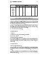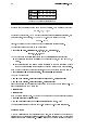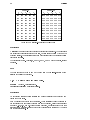
1
Notes on S-PLUS:
A Programming Environment for
Data Analysis and Graphics
Bill Venables and Dave Smith
Department of Statistics
The University of Adelaide
Email: [email protected]
c W. Venables, 1990, 1992.
Version 2.1, July, 1992
Preface
These notes were originally intended only for local consumption at the University of
Adelaide, South Australia. After some encouraging comments from students, the author
decided to release them to a larger readership in the hope that in some small way they
promote good data analysis. S (or S-PLUS) is no panacea, of course, but in oering
simply a coherent suite of general and exible tools to devise precisely the right kind of
analysis, rather than a collection of packaged standard analyses, in my view it represents
the single complete environment most conducive to good data analysis so far available.
Some evidence of the local origins of these notes is still awkwardly apparent. For example
they use the Tektronics graphics emulations on terminals and workstations, which at
the time of writing is still the only one available to the author. The X11 windowing
system, which allows separate windows for characters and graphics simultaneously to be
displayed, is much to be preferred and it will be used in later versions. Also the local
audience would be very familiar with MINITAB, MATLAB, Glim and Genstat, and various
echoes of these persist. At one point some passing acquaintance with the Australian
States is assumed, but the elementary facts are given in a footnote for foreign readers.
Comments and corrections are always welcome. Please address email correspondence to
the author at [email protected].
The author is indebted to many people for useful contributions, but in particular Lucien
W. Van Elsen, who did the basic TEX to LaTEX conversion and Rick Becker who oered
an authoritative and extended critique on an earlier version. Responsibility for this
version, however, remains entirely with the author, and the notes continue to enjoy a
fully unocial and unencumbered status.
These notes may be freely copied and redistributed for any educational purpose provided
the copyright notice remains intact. Where appropriate, a small charge to cover the costs
of production and distribution, only, may be made.
Bill Venables,
University of Adelaide,
16th December, 1990.
Addendum: Version 2.0, April 1992
As foreshadowed above the present version of the notes contains references to the use
of S in a workstation environment, although I hope they remain useful to the user on
an ordinary graphics terminal. Of much greater importance, however, are the language
developments that have taken place in S itself in the August 1991 release. These are
only partially addressed in this version of the notes, as a complete coverage would require
a document of much greater length than was ever intended. I trust however that the
sketches given here are useful and a spur to the reader to seek further enlightenment in
the standard reference materials.
The present notes are also centred around S-PLUS rather than plain vanilla S. This
simply reects a change in the implementation of S made available to my students and
me by my employer. It should not be read as any sort of endorsement one way or another.
My sincere thanks to David Smith, James Pearce and Ron Baxter for many useful suggestions.
Bill Venables,
University of Adelaide,
13th April, 1992.
i
Contents
Preface
i
1 Introduction and Preliminaries
1
1.1
1.2
1.3
1.4
1.5
1.6
1.7
1.8
Reference manuals : : : : : : : : : : : : : : : : : : : : :
S-PLUS and X{windows : : : : : : : : : : : : : : : : : :
Using S-PLUS interactively : : : : : : : : : : : : : : : :
An introductory session : : : : : : : : : : : : : : : : : :
S-PLUS and UNIX : : : : : : : : : : : : : : : : : : : : :
Getting help with functions and features : : : : : : : : :
S-PLUS commands. Case sensitivity. : : : : : : : : : : :
Recall and correction of previous commands : : : : : : :
1.8.1 S-PLUS : : : : : : : : : : : : : : : : : : : : : : :
1.8.2 Vanilla S : : : : : : : : : : : : : : : : : : : : : :
1.9 Executing commands from, or diverting output to, a le
1.10 Data directories. Permanency. Removing objects. : : : :
:
:
:
:
:
:
:
:
:
:
:
:
:
:
:
:
:
:
:
:
:
:
:
:
:
:
:
:
:
:
:
:
:
:
:
:
:
:
:
:
:
:
:
:
:
:
:
:
:
:
:
:
:
:
:
:
:
:
:
:
:
:
:
:
:
:
:
:
:
:
:
:
:
:
:
:
:
:
:
:
:
:
:
:
:
:
:
:
:
:
:
:
:
:
:
:
:
:
:
:
:
:
:
:
:
:
:
:
:
:
:
:
:
:
:
:
:
:
:
:
2 Simple manipulations; numbers and vectors
2.1
2.2
2.3
2.4
2.5
2.6
2.7
6
Vectors : : : : : : : : : : : : : : : : : : : : : : : : : : : : :
Vector arithmetic : : : : : : : : : : : : : : : : : : : : : : : :
Generating regular sequences : : : : : : : : : : : : : : : : :
Logical vectors : : : : : : : : : : : : : : : : : : : : : : : : :
Missing values : : : : : : : : : : : : : : : : : : : : : : : : : :
Character vectors : : : : : : : : : : : : : : : : : : : : : : : :
Index vectors. Selecting and modifying subsets of a data set
:
:
:
:
:
:
:
:
:
:
:
:
:
:
:
:
:
:
:
:
:
:
:
:
:
:
:
:
:
:
:
:
:
:
:
:
:
:
:
:
:
:
:
:
:
:
:
:
:
:
:
:
:
:
:
:
3 Objects, their modes and attributes
3.1 Intrinsic attributes: mode and length :
3.2 Changing the length of an object : : :
3.3 attributes() and attr() : : : : : : :
3.4 The class of an object : : : : : : : : :
4 Categories and factors
1
1
2
2
3
3
3
4
4
4
4
5
6
6
7
8
8
8
9
11
:
:
:
:
:
:
:
:
:
:
:
:
:
:
:
:
:
:
:
:
:
:
:
:
:
:
:
:
:
:
:
:
:
:
:
:
:
:
:
:
:
:
:
:
:
:
:
:
:
:
:
:
:
:
:
:
:
:
:
:
:
:
:
:
:
:
:
:
:
:
:
:
:
:
:
:
:
:
:
:
11
12
12
12
13
4.1 A specic example : : : : : : : : : : : : : : : : : : : : : : : : : : : : : : : 13
4.2 The function tapply() and ragged arrays : : : : : : : : : : : : : : : : : : 14
ii
5 Arrays and matrices
5.1
5.2
5.3
5.4
5.5
5.6
5.7
5.8
5.9
5.10
16
Arrays : : : : : : : : : : : : : : : : : : : : : : : : : : : : : : : : : : : : :
Array indexing. Subsections of an array : : : : : : : : : : : : : : : : : :
Index arrays : : : : : : : : : : : : : : : : : : : : : : : : : : : : : : : : : :
The array() function : : : : : : : : : : : : : : : : : : : : : : : : : : : :
5.4.1 Mixed vector and array arithmetic. The recycling rule : : : : : :
The outer product of two arrays : : : : : : : : : : : : : : : : : : : : : :
5.5.1 An example: Determinants of 2 2 digit matrices : : : : : : : :
Generalized transpose of an array : : : : : : : : : : : : : : : : : : : : : :
Matrix facilities. Multiplication, inversion and solving linear equations. :
Forming partitioned matrices. cbind() and rbind(). : : : : : : : : : :
The concatenation function, c(), with arrays. : : : : : : : : : : : : : : :
Frequency tables from factors. The table() function : : : : : : : : : : :
:
:
:
:
:
:
:
:
:
:
:
:
6 Lists, data frames, and their uses
16
16
16
18
18
19
19
19
20
21
21
21
23
6.1 Lists : : : : : : : : : : : : : : : : : : : : : : : : : : : : :
6.2 Constructing and modifying lists : : : : : : : : : : : : :
6.2.1 Concatenating lists : : : : : : : : : : : : : : : : :
6.3 Some functions returning a list result : : : : : : : : : : :
6.3.1 Eigenvalues and eigenvectors : : : : : : : : : : :
6.3.2 Singular value decomposition and determinants :
6.3.3 Least squares tting and the QR decomposition
6.4 Data frames : : : : : : : : : : : : : : : : : : : : : : : : :
6.4.1 Making data frames : : : : : : : : : : : : : : : :
6.4.2 attach() and detach() : : : : : : : : : : : : : :
6.4.3 Working with data frames : : : : : : : : : : : : :
6.4.4 Attaching arbitrary lists : : : : : : : : : : : : : :
:
:
:
:
:
:
:
:
:
:
:
:
:
:
:
:
:
:
:
:
:
:
:
:
7 Reading data from les
:
:
:
:
:
:
:
:
:
:
:
:
:
:
:
:
:
:
:
:
:
:
:
:
:
:
:
:
:
:
:
:
:
:
:
:
:
:
:
:
:
:
:
:
:
:
:
:
:
:
:
:
:
:
:
:
:
:
:
:
:
:
:
:
:
:
:
:
:
:
:
:
:
:
:
:
:
:
:
:
:
:
:
:
:
:
:
:
:
:
:
:
:
:
:
:
23
23
24
24
24
24
25
25
26
26
26
27
28
7.1 The scan() function : : : : : : : : : : : : : : : : : : : : : : : : : : : : : : 28
7.2 The read.table() function : : : : : : : : : : : : : : : : : : : : : : : : : : 28
7.3 Other facilities; editing data : : : : : : : : : : : : : : : : : : : : : : : : : : 29
8 More language features. Loops and conditional execution
30
8.1 Grouped expressions : : : : : : : : : : : : : : : : : : : : : : : : : : : : : : 30
8.2 Control statements : : : : : : : : : : : : : : : : : : : : : : : : : : : : : : : 30
iii
9 Writing your own functions
9.1
9.2
9.3
9.4
9.5
9.6
Dening new binary operators. : : : : : : : : : : :
Named arguments and defaults. \: : :" : : : : : : :
Assignments within functions are local. Frames. : :
More advanced examples : : : : : : : : : : : : : : :
Customizing the environment. .First and .Last :
Classes, generic functions and object orientation :
10 Statistical models in S-PLUS
10.1
10.2
10.3
10.4
10.5
10.6
10.7
10.8
:
:
:
:
:
:
:
:
:
:
:
:
:
:
:
:
:
:
Dening statistical models; formul : : : : : : : : : : :
Regression models; tted model objects : : : : : : : : :
Generic functions for extracting information : : : : : : :
Analysis of variance; comparing models : : : : : : : : :
10.4.1 ANOVA tables : : : : : : : : : : : : : : : : : : :
Updating tted models. The ditto name \." : : : : : :
Generalized linear models; families : : : : : : : : : : : :
10.6.1 Families : : : : : : : : : : : : : : : : : : : : : : :
10.6.2 The glm() function : : : : : : : : : : : : : : : :
Nonlinear regression models; parametrized data frames :
10.7.1 Changes to the form of the model formula : : : :
10.7.2 Specifying the parameters : : : : : : : : : : : : :
Some non-standard models : : : : : : : : : : : : : : : :
11 Graphical procedures
:
:
:
:
:
:
:
:
:
:
:
:
:
:
:
:
:
:
:
:
:
:
:
:
:
:
:
:
:
:
:
:
:
:
:
:
:
:
:
:
:
:
:
:
:
:
:
:
:
:
:
:
:
:
:
:
:
11.1 High-level plotting commands : : : : : : : : : : : : : : : : : :
11.1.1 The plot() function : : : : : : : : : : : : : : : : : : :
11.1.2 Displaying multivariate data : : : : : : : : : : : : : :
11.1.3 Display graphics : : : : : : : : : : : : : : : : : : : : :
11.1.4 Arguments to high-level plotting functions : : : : : : :
11.2 Low-level plotting commands : : : : : : : : : : : : : : : : : :
11.3 Interactive graphics functions : : : : : : : : : : : : : : : : : :
11.4 Using graphics parameters : : : : : : : : : : : : : : : : : : : :
11.4.1 Permanent changes: the par() function : : : : : : : :
11.4.2 Temporary changes: arguments to graphics functions :
11.5 Graphics parameters list : : : : : : : : : : : : : : : : : : : : :
11.5.1 Graphical elements : : : : : : : : : : : : : : : : : : : :
11.5.2 Axes and Tick marks : : : : : : : : : : : : : : : : : : :
iv
:
:
:
:
:
:
:
:
:
:
:
:
:
:
:
:
:
:
:
:
:
:
:
:
:
:
:
:
:
:
:
:
:
:
:
:
:
:
:
:
:
:
:
:
:
:
:
:
:
:
:
:
:
:
:
:
:
:
:
:
:
:
:
:
:
:
:
:
:
:
:
:
:
:
:
:
:
:
:
:
:
:
:
:
:
:
:
:
:
:
:
:
:
:
:
:
:
:
:
:
:
:
:
:
:
:
:
:
:
:
:
:
:
:
:
:
:
:
:
:
:
:
:
:
:
:
:
:
:
:
:
:
:
:
:
:
:
:
:
:
:
:
:
:
:
:
:
:
:
:
:
:
:
:
:
:
:
:
:
:
:
:
:
:
:
:
:
:
:
:
:
:
:
:
:
:
:
:
:
:
:
:
:
:
:
:
:
:
:
:
:
:
:
:
:
:
:
:
:
:
:
:
:
:
:
:
:
:
:
:
:
:
:
:
:
:
:
:
:
:
:
:
:
:
31
31
32
32
33
35
36
37
37
38
39
39
40
41
41
42
42
45
45
46
47
48
48
48
49
49
50
51
52
53
53
54
54
54
55
A S-PLUS: An Introductory Session
61
B The Inbuilt Command Line Editor in S-PLUS
64
C Exercises
66
B.1 Preliminaries : : : : : : : : : : : : : : : : : : : : : : : : : : : : : : : : : : 64
B.2 Editing Actions : : : : : : : : : : : : : : : : : : : : : : : : : : : : : : : : : 64
B.3 Command Line Editor Summary : : : : : : : : : : : : : : : : : : : : : : : 65
C.1 The Cloud Point Data : : : : : : : : : : : : :
C.2 The Janka Hardness Data : : : : : : : : : : :
C.3 The Tuggeranong House Price Data : : : : :
C.4 Yorke Penninsula Wheat Data : : : : : : : :
C.5 The Iowa Wheat Yield Data : : : : : : : : : :
C.6 The Gasoline Yield Data : : : : : : : : : : : :
C.7 The Michaelson-Morley Speed of Light Data :
C.8 The Rat Genotype Data : : : : : : : : : : : :
C.9 Fisher's Sugar Beet Data : : : : : : : : : : :
C.10 A Barley Split Plot Field Trial. : : : : : : : :
C.11 The Snail Mortality Data : : : : : : : : : : :
C.12 The Kalythos Blindness Data : : : : : : : : :
C.13 The Stormer Viscometer Data : : : : : : : : :
C.14 The Chlorine availability data : : : : : : : : :
C.15 The Saturated Steam Pressure Data : : : : :
C.16 Count Rumford's Friction Data : : : : : : : :
C.17 The Jellysh Data. : : : : : : : : : : : : : : :
C.18 Archaelogical Pottery Data : : : : : : : : : :
C.19 The Beaujolais Quality Data : : : : : : : : :
C.20 The Painter's Data of de Piles : : : : : : : : :
v
:
:
:
:
:
:
:
:
:
:
:
:
:
:
:
:
:
:
:
:
:
:
:
:
:
:
:
:
:
:
:
:
:
:
:
:
:
:
:
:
:
:
:
:
:
:
:
:
:
:
:
:
:
:
:
:
:
:
:
:
:
:
:
:
:
:
:
:
:
:
:
:
:
:
:
:
:
:
:
:
:
:
:
:
:
:
:
:
:
:
:
:
:
:
:
:
:
:
:
:
:
:
:
:
:
:
:
:
:
:
:
:
:
:
:
:
:
:
:
:
:
:
:
:
:
:
:
:
:
:
:
:
:
:
:
:
:
:
:
:
:
:
:
:
:
:
:
:
:
:
:
:
:
:
:
:
:
:
:
:
:
:
:
:
:
:
:
:
:
:
:
:
:
:
:
:
:
:
:
:
:
:
:
:
:
:
:
:
:
:
:
:
:
:
:
:
:
:
:
:
:
:
:
:
:
:
:
:
:
:
:
:
:
:
:
:
:
:
:
:
:
:
:
:
:
:
:
:
:
:
:
:
:
:
:
:
:
:
:
:
:
:
:
:
:
:
:
:
:
:
:
:
:
:
:
:
:
:
:
:
:
:
:
:
:
:
:
:
:
:
:
:
:
:
:
:
:
:
:
:
:
:
:
:
:
:
:
:
:
:
:
:
:
:
:
:
:
:
:
:
:
:
:
:
:
:
:
:
:
:
:
:
:
:
:
:
:
:
:
:
66
66
67
67
67
68
69
71
71
72
73
74
76
76
77
78
79
79
80
80
Introduction and Preliminaries
1
1 Introduction and Preliminaries
S-PLUS is an integrated suite of software facilities for data manipulation, calculation and
graphical display. Among other things it has
an eective data handling and storage facility,
a suite of operators for calculations on arrays, in particular matrices,
a large, coherent, integrated collection of intermediate tools for data analysis,
graphical facilities for data analysis and display either at a workstation or on hardcopy, and
a well developed, simple and eective programming language which includes conditionals, loops, user dened recursive functions and input and output facilities.
(Indeed most of the system supplied functions are themselves written in the S-PLUS
language.)
The term \environment" is intended to characterize it as a fully planned and coherent
system, rather than an incremental accretion of very specic and inexible tools, as is
frequently the case with other data analysis software.
S-PLUS is very much a vehicle for newly developing methods of interactive data analysis.
As such it is very dynamic, and new releases have not always been fully upwardly compatible with previous releases. Some users welcome the changes because of the bonus of
new technology and new methods that come with new releases; others seem to be more
worried by the fact that old code no longer works. Although S-PLUS is intended as a
programming language, in my view one should regard programmes written in S-PLUS as
essentially ephemeral.
The name S (or S-PLUS), as with many names within the UNIX world, is not explained,
but left as a cryptic puzzle, and probably a weak pun. However its authors insist it does
not stand for \Statistics"!
These notes will be mainly concerned with S-PLUS, an enhanced version of S distributed
by Statistical Sciences, Inc., Seattle, Washington.
1.1 Reference manuals
The basic reference is The New S Language: A Programming Environment for Data
Analysis and Graphics by Richard A. Becker, John M. Chambers and Allan R. Wilks.
The new features of the August 1991 release of S are covered in Statistical Models in S
Edited by John M. Chambers and Trevor J. Hastie. In addition there are specically
S-PLUS reference books: S-PLUS User's Manual (Volumes 1 & 2) and S-PLUS Reference
Manual (in two volumes, A{K and L{Z).
It is not the intention of these notes to replace these manuals. Rather these notes are
intended as a brief introduction to the S-PLUS programming language and a minor
amplication of some important points. Ultimately the user of S-PLUS will need to
consult this reference manual, probably frequently.
1.2
S-PLUS
and windows
X{
The most convenient way to use S-PLUS is at a high quality graphics workstation running
a windowing system. Since these are becoming more readily available, these notes are
aimed at users who have this facility. In particular we will occasionally refer to the use
of S-PLUS on an X{window system, and even with the motif window manager, although
2
Introduction and Preliminaries
the vast bulk of what is said applies generally to any implementation of the S-PLUS
environment.
Setting up a workstation to take full advantage of the customizable features of S-PLUS
is a straightforward if somewhat tedious procedure, and will not be considered further
here. Users in diculty should seek local expert help.
1.3 Using
S-PLUS
interactively
When you use the S-PLUS program it issues a prompt when it expects input commands.
The default prompt is \>", which is sometimes the same as the shell prompt, and so it
may appear that nothing is happening. However, as we shall see, it is easy to change
to a dierent S-PLUS prompt if you wish. In these notes we will assume that the shell
prompt is \$".
In using S-PLUS the suggested procedure for the rst occasion is as follows:
1. Create a separate sub-directory, say work, to hold data les on which you will use
S-PLUS for this problem. This will be the working directory whenever you use
S-PLUS for this particular problem.
$ mkdir work
$ cd work
2. Place any data les you wish to use with S-PLUS in work.
3. Create a sub-directory of work called .Data for use by S-PLUS.
$ mkdir .Data
4. Start the S-PLUS program with the command
$ Splus -e
5. At this point S-PLUS commands may be issued (see later).
6. To quit the S-PLUS program the command is
> q()
$
The procedure is simpler using S-PLUS after the rst time:
Make work the working directory and start the program as before:
$ cd work
$ Splus -e
Use the S-PLUS program, terminating with the q() command at the end of the session.
1.4 An introductory session
Readers wishing to get a feel for S-PLUS at a workstation (or terminal) before proceeding are strongly advised to work through the model introductory session given in
Appendix A, starting on page 61.
1.5 S-PLUS and UNIX
1.5
S-PLUS
and
3
UNIX
S-PLUS allows escape to the operating system at any time in the session. If a command,
on a new line, begins with an exclamation mark then the rest of the line is interpreted
as a UNIX command. So for example to look through a data le without leaving S-PLUS
you could use
> !more curious.dat
When you nish paging the le the S-PLUS session is resumed.
In fact the integration of S-PLUS into UNIX is very complete. For example, there is a
command, unix(: : : ), that executes any unix command, (specied as a character string
argument), and passes on any output from the command as a character string to the
program. Essentially the full power of the operating system remains easily available to
the user of the S-PLUS program during any session.
There are non-UNIX implementations of S-PLUS, for example for DOS. Users should
consult the appropriate user guides for more information.
1.6 Getting help with functions and features
S-PLUS has an inbuilt help facility similar to the
man facility of UNIX. To get more
information on any specic named function, for example solve the command is
> help(solve)
An alternative is
> ?solve
For a feature specied by special characters, the argument must be enclosed in double
quotes, making it a `character string':
> help("[[")
A much more comprehensive help facility is available with the X{windows version of
S-PLUS The command
> help.start(gui="motif")
causes a \help window" to appear (with the \motif" graphical user interface). It is at
this point possible to select items interactively from a series of menus, and the selection
process again causes other windows to appear with the help information. This may be
either scanned at the screen and dismissed, or sent to a printer for hardcopy, or both.
1.7
S-PLUS
commands. Case sensitivity.
Technically S-PLUS is a function language with a very simple syntax. It is case sensitive
as are most UNIX based packages, so A and a are dierent variables.
Elementary commands consist of either expressions or assignments. If an expression is
given as a command, it is evaluated, printed, and the value is lost. An assignment also
evaluates an expression and passes the value to a variable but the result is not printed
automatically.
Commands are separated either by a semi-colon, ;, or by a newline. If a command is
not complete at the end of a line, S-PLUS will give a dierent prompt, for example
4
Introduction and Preliminaries
on second and subsequent lines and continue to read input until the command is syntactically complete. This prompt may also be changed if the user wishes. In these notes
we will generally omit the continuation prompt and indicate continuation by simple
indenting.
1.8 Recall and correction of previous commands
1.8.1 S-PLUS
S-PLUS (but not plain S) provides a mechanism for recall and correction of previous
commands. For interactive use this is a vital facility and greatly increases the productive
output of most people. To invoke S-PLUS with the command recall facility enabled use
the -e ag:
> Splus -e
Within the session, command recall is available using either emacs-style or vi-style commands. The former is very similar to command recall with an interactive shell such
as tcsh. Details are given in Appendix B of these notes, or they may be found in the
reference manual or the online help documents.
1.8.2 Vanilla S
With S no built-in mechanism is available, but there are two common ways of obtaining
command recall for interactive sessions.
Run the S session under emacs using S{mode, a major mode designed to support
S. This is probably more convenient than even the inbuilt editor of S-PLUS in the
long term, however it does require a good deal of preliminary eort for persons not
familiar with the emacs editor. It also often requires a dedicated workstation with
a good deal of memory and other resources.
Run the S session under some front end processor, such as the public domain fep
program, available from the public sources archives. This provides essentially the
same service as the inbuilt S-PLUS editor, but with somewhat more overhead, (but
a great deal less overhead than emacs requires.)
1.9 Executing commands from, or diverting output to, a le
If commands are stored on an external le, say commands.S in the working directory
work, they may be executed at any time in an S-PLUS session with the command
> source("commands.S")
Similarly
> sink("record.lis")
will divert all subsequent output from the terminal to an external le, record.lis. The
command
> sink()
restores it to the terminal once again.
1.10 Data directories. Permanency. Removing objects.
5
1.10 Data directories. Permanency. Removing objects.
All objects created during your S-PLUS sessions are stored, in a special form, in the
.Data sub-directory of your working directory work, say.
Each object is held as a separate le of the same name and so may be manipulated by
the usual UNIX commands such as rm, cp and mv. This means that if you resume your
S-PLUS session at a later time, objects created in previous sessions are still available,
which is a highly convenient feature.
This also explains why it is recommended that you should use separate working directories for dierent jobs. Common names for objects are single letter names like x, y and
so on, and if two problems share the same .Data sub-directory the objects will become
mixed up and you may overwrite one with another.
There is, however, another method of partitioning variables within the same .Data directory using data frames. These are discussed further in x6.4.
In S-PLUS, to get a list of names of the objects currently dened use the command
> objects()
whose result is a vector of character strings giving the names.
When S-PLUS looks for an object, it searches in turn through a sequence of places known
as the search list. Usually the rst entry in the search list is the .Data sub-directory of
the current working directory. The names of the places currently on the search list are
displayed by the function
> search()
The names of the objects held in any place in the search list can be displayed by giving
the objects() function an argument. For example
> objects(2)
lists the contents of the entity at position 2 of the search list. The search list can contain
either data frames and allies, which are themselves internal S-PLUS objects, as well as
directories of les which are UNIX objects.
Extra entities can be added to this list with the attach() function and removed with
the detach() function, details of which can be found in the manual or the help facility.
To remove objects permanently the function rm is available:
> rm(x, y, z, ink, junk, temp, foo, bar)
The function remove() can be used to remove objects with non-standard names. Also
the ordinary UNIX facility, rm, may be used to remove the appropriate les in the .Data
directory, as mentioned above.
6
Simple manipulations; numbers and vectors
2 Simple manipulations; numbers and vectors
2.1 Vectors
S-PLUS operates on named data structures. The simplest such structure is the vector,
which is a single entity consisting of an ordered collection of numbers. To set up a vector
named x, say, consisting of ve numbers, namely 10:4, 5:6, 3:1, 6:4 and 21:7, use the
S-PLUS command
> x <- c(10.4, 5.6, 3.1, 6.4, 21.7)
This is an assignment statement using the function c() which in this context can take an
arbitrary number of vector arguments and whose value is a vector got by concatenating
its arguments end to end.1
A number occurring by itself in an expression is taken as a vector of length one.
Notice that the assignment operator is not the usual = operator, which is reserved for
another purpose. It consists of the two characters < (`less than') and - (`minus') occurring
strictly side-by-side and it `points' to the structure receiving the value of the expression.
Assignments can also be made in the other direction, using the obvious change in the
assignment operator. So the same assignment could be made using
> c(10.4, 5.6, 3.1, 6.4, 21.7) -> x
If an expression is used as a complete command, the value is printed and lost. So now
if we were to use the command
> 1/x
the reciprocals of the ve values would be printed at the terminal (and the value of x,
of course, unchanged).
The further assignment
> y <- c(x, 0, x)
would create a vector y with 11 entries consisting of two copies of x with a zero in the
middle place.
2.2 Vector arithmetic
Vectors can be used in arithmetic expressions, in which case the operations are performed
element by element. Vectors occurring in the same expression need not all be of the same
length. If they are not, the value of the expression is a vector with the same length as
the longest vector which occurs in the expression. Shorter vectors in the expression
are recycled as often as need be (perhaps fractionally) until they match the length of
the longest vector. In particular a constant is simply repeated. So with the above
assignments the command
> v <- 2*x + y + 1
generates a new vector v of length 11 constructed by adding together, element by element,
2*x repeated 2:2 times, y repeated just once, and 1 repeated 11 times.
The elementary arithmetic operators are the usual +, -, *, / and ^ for raising to a power.
In addition all of the common arithmetic functions are available. log, exp, sin, cos,
tan, sqrt, and so on, all have their usual meaning. max and min select the largest and
smallest elements of an vector respectively. range is a function whose value is a vector
1 With other than vector types of argument, such as list mode arguments, the action of c() is at
rst sight rather dierent. See x6.2.1.
2.3 Generating regular sequences
7
of length two, namely c(min(x), max(x)). length(x) is the number of elements in x,
sum(x) gives the total of the elements in x and prod(x) their product.
Two statistical functions are mean(x) which calculates the sample mean, which is the
same as sum(x)/length(x), and var(x) which gives
sum((x-mean(x))^2)/(length(x)-1)
or sample variance. If the argument to var() is an n p matrix the value is a p p
sample covariance matrix got by regarding the rows as independent p variate sample
vectors.
sort(x) returns a vector of the same size as x with the elements arranged in increasing
order; however there are other more exible sorting facilities available (see order() or
sort.list() which produce a permutation to do the sorting).
rnorm(x) is a function which generates a vector (or more generally an array) of pseudorandom standard normal deviates, of the same size as x.
2.3 Generating regular sequences
S-PLUS has a number of facilities for generating commonly used sequences of numbers.
For example 1:30 is the vector c(1,2, : : : ,29,30). The colon operator has highest
priority within an expression, so, for example 2*1:15 is the vector c(2,4,6, : : : ,28,30).
Put n <- 10 and compare the sequences 1:n-1 and 1:(n-1).
The construction 30:1 may be used to generate a sequence backwards.
The function seq() is a more general facility for generating sequences. It has ve arguments, only some of which may be specied in any one call. The rst two arguments,
if given, specify the beginning and end of the sequence, and if these are the only two
arguments given the result is the same as the colon operator. That is seq(2,10) is the
same vector as 2:10.
Parameters to seq(), and to many other S-PLUS functions, can also be given in named
form, in which case the order in which they appear is irrelevant. The rst two parameters
may be named from=value and to=value; thus seq(1,30), seq(from=1, to=30) and
seq(to=30, from=1) are all the same as 1:30. The next two parameters to seq() may
be named by=value and length=value, which specify a step size and a length for the
sequence respectively. If neither of these is given, the default by=1 is assumed.
For example
> seq(-5, 5, by=.2) -> s3
generates in s3 the vector c(-5.0,
-4.8, -4.6,
:::,
4.6, 4.8, 5.0)
. Similarly
> s4 <- seq(length=51, from=-5, by=.2)
generates the same vector in s4.
The fth parameter may be named along=vector, which if used must be the only parameter, and creates a sequence 1, 2, : : : , length(vector ), or the empty sequence if
the vector is empty (as it can be).
A related function is rep() which can be used for replicating a structure in various
complicated ways. The simplest form is
> s5 <- rep(x, times=5)
which will put ve copies of x end-to-end in s5.
8
Simple manipulations; numbers and vectors
2.4 Logical vectors
As well as numerical vectors, S-PLUS allows manipulation of logical quantities. The
elements of a logical vectors have just two possible values, represented formally as F (for
`false') and T (for `true').
Logical vectors are generated by conditions. For example
> temp <- x>13
sets temp as a vector of the same length as x with values F corresponding to elements of
x where the condition is not met and T where it is.
The logical operators are <, <=, >, >=, == for exact equality and != for inequality. In
addition if c1 and c2 are logical expressions, then c1 & c1 is their intersection, c1 | c2 is
their union and ! c1 is the negation of c1.
Logical vectors may be used in ordinary arithmetic, in which case they are coerced into
numeric vectors, F becoming 0 and T becoming 1. However there are situations where
logical vectors and their coerced numeric counterparts are not equivalent, for example
see the next subsection.
2.5 Missing values
In some cases the components of a vector may not be completely known. When an
element or value is \not available" or a \missing value" in the statistical sense, a place
within a vector may be reserved for it by assigning it the special value NA. In general
any operation on an NA becomes an NA. The motivation for this rule is simply that if the
specication of an operation is incomplete, the result cannot be known and hence is not
available.
The function is.na(x) gives a logical vector of the same size as x with value T if and
only if the corresponding element in x is NA.
> ind <- is.na(z)
Notice that the logical expression x == NA is quite dierent from is.na(x) since NA is
not really a value but a marker for a quantity that is not available. Thus x == NA is a
vector of the same length as x all of whose values are NA as the logical expression itself
is incomplete and hence undecidable.
2.6 Character vectors
Character quantities and character vectors are used frequently in S-PLUS, for example
as plot labels. Where needed they are denoted by a sequence of characters delimited by
the double quote character. E. g. "x-values", "New iteration results".
Character vectors may be concatenated into a vector by the c() function; examples of
their use will emerge frequently.
The paste() function takes an arbitrary number of arguments and concatenates them
into a single character string. Any numbers given among the arguments are coerced
into character strings in the evident way, that is, in the same way they would be if they
were printed. The arguments are by default separated in the result by a single blank
character, but this can be changed by the named parameter, sep=string, which changes
it to string, possibly empty.
For example
> labs <- paste(c("X","Y"), 1:10, sep="")
2.7 Index vectors. Selecting and modifying subsets of a data set
9
makes labs into the character vector
("X1", "Y2", "X3", "Y4", "X5", "Y6", "X7", "Y8", "X9", "Y10")
Note particularly that recycling of short lists takes place here too; thus c("X",
repeated 5 times to match the sequence 1:10.
"Y")
is
2.7 Index vectors. Selecting and modifying subsets of a data set
Subsets of the elements of a vector may be selected by appending to the name of the
vector an index vector in square brackets. More generally any expression that evaluates
to a vector may have subsets of its elements similarly selected be appending an index
vector in square brackets immediately after the expression.
Such index vectors can be any of four distinct types.
1. A logical vector. In this case the index vector must be of the same length as the
vector from which elements are to be selected. Values corresponding to T in the
index vector are selected and those corresponding to F omitted. For example
> y <- x[!is.na(x)]
creates (or re-creates) an object y which will contain the non-missing values of x,
in the same order. Note that if x has missing values, y will be shorter than x. Also
> (x+1)[(!is.na(x)) & x>0] -> z
creates an object z and places in it the values of the vector x+1 for which the
corresponding value in x was both non-missing and positive.
2. A vector of positive integral quantities. In this case the values in the index vector must lie in the the set f1, 2, : : : , length(x)g. The corresponding elements
of the vector are selected and concatenated, in that order, in the result. The index
vector can be of any length and the result is of the same length as the index vector.
For example x[6] is the sixth component of x and
> x[1:10]
selects the rst 10 elements of x, (assuming length(x) 10). Also
> c("x","y")[rep(c(1,2,2,1), times=4)]
(an admittedly unlikely thing to do) produces a character vector of length 16
consisting of "x", "y", "y", "x" repeated four times.
3. A vector of negative integral quantities. Such an index vector species the values to be excluded rather than included. Thus
> y <- x[-(1:5)]
gives y all but the rst ve elements of x.
4. A vector of character strings. This possibility only applies where an object has
a names attribute to identify its components. In this case a subvector of the names
vector may be used in the same way as the positive integral labels in 2. above.
> lunch <- fruit[c("apple","orange")]
This option is particularly useful in connection with data frames, as we shall see
later.
An indexed expression can also appear on the receiving end of an assignment, in which
case the assignment operation is performed only on those elements of the vector. The
10
Simple manipulations; numbers and vectors
expression must be of the form vector[index vector ] as having an arbitrary expression
in place of the vector name does not make much sense here.
The vector assigned must match the length of the index vector, and in the case of a
logical index vector it must again be the same length as the vector it is indexing.
For example
> x[is.na(x)] <- 0
replaces any missing values in x by zeros and
> y[y<0] <- -y[y<0]
has the same eect as
> y <- abs(y)2
2 Note that abs() does not work as expected with complex arguments. The appropriate function for
the complex modulus is Mod().
Objects, their modes and attributes
11
3 Objects, their modes and attributes
3.1 Intrinsic attributes: mode and length
The entities S-PLUS operates on are technically known as objects. Examples are vectors
of numeric (real) or complex values, vectors of logical values and vectors of character
strings. These are known as `atomic' structures since their components are all of the
same type, or mode, namely numeric 3, complex, logical and character respectively.
Vectors must have their values all of the same mode. Thus any given vector must be
unambiguously either logical, numeric, complex or character. The only mild exception
to this rule is the special \value" listed as NA for quantities not available. Note that
a vector can be empty and still have a mode. For example the empty character string
vector is listed as character(0) and the empty numeric vector as numeric(0).
S-PLUS also operates on objects called lists, which are of mode list. These are ordered
sequences of objects which individually can be of any mode. lists are known as `recursive'
rather than atomic structures since their components can themselves be lists in their own
right.
The other recursive structures are those of mode function and expression. Functions
are the functions that form part of the S-PLUS system along with similar user written
functions, which we discuss in some detail later in these notes. Expressions as objects
form an advanced part of S-PLUS which will not be discussed in these notes, except
indirectly when we discuss formul with we discuss modelling in S-PLUS.
By the mode of an object we mean the basic type of its fundamental constituents. This
is a special case of an attribute of an object. The attributes of an object provide specic
information about the object itself. Another attribute of every object is its length. The
functions mode(object) and length(object) can be used to nd out the mode and length
of any dened structure.
For example, if z is complex vector of length 100, then in an expression mode(z) is the
character string "complex" and length(z) is 100.
S-PLUS caters for changes of mode almost anywhere it could be considered sensible to
do so, (and a few where it might not be). For example with
> z <- 0:9
we could put
> digits <- as.character(z)
after which digits is the character vector ("0", "1", "2", : : : , "9"). A further
coercion, or change of mode, reconstructs the numerical vector again:
> d <- as.numeric(digits)
Now
and
are the same.4 There is a large collection of functions of the form
for either coercion from one mode to another, or for investing an object
with some other attribute it may not already posses. The reader should consult the help
le to become familiar with them.
d
z
as.something()
3 numeric mode is actually an amalgam of three distinct modes, namely integer, single precision and
double precision, as explained in the manual.
4 In general coercion from numeric to character and back again will not be exactly reversible, because
of roundo errors in the character representation.
12
Objects, their modes and attributes
3.2 Changing the length of an object
An \empty" object may still have a mode. For example
> e <- numeric()
makes e an empty vector structure of mode numeric. Similarly character() is a empty
character vector, and so on. Once an object of any size has been created, new components
may be added to it simply by giving it an index value outside its previous range. Thus
> e[3] <- 17
now makes e a vector of length 3, (the rst two components of which are at this point
both NA). This applies to any structure at all, provided the mode of the additional
component(s) agrees with the mode of the object in the rst place.
This automatic adjustment of lengths of an object is used often, for example in the
scan() function for input.
Conversely to truncate the size of an object requires only an assignment to do so. Hence
if alpha is a structure of length 10, then
> alpha <- alpha[2 * 1:5]
makes it an object of length 5 consisting of just the former components with even index.
The old indices are not retained, of course.
3.3
attributes()
and attr()
The function attributes(object) gives a list of all the non-intrinsic attributes currently
dened for that object. The function attr(object,name ) can be used to select a specic
attribute. These functions are rarely used, except in rather special circumstances when
some new attribute is being created for some particular purpose, for example to associate
a creation date or an operator with an S-PLUS object. The concept, however, is very
important.
3.4 The class of an object
A special attribute known as the class of the object has been introduced in the August 1991 release of S and S-PLUS to allow for an object oriented style of programming
in S-PLUS.
For example if an object has class data.frame, it will be printed in a certain way, the
plot() function will display it graphically in a certain way, and other generic functions
such as summary() will react to it as an argument in a way sensitive to its class.
To remove temporarily the eects of class, use the function unclass(). For example if
winter has the class data.frame then
> winter
will print it in data frame form, which is rather like a matrix, whereas
> unclass(winter)
will print it as an ordinary list. Only in rather special situations do you need to use this
facility, but one is when you are learning to come to terms with the idea of class and
generic functions.
Generic functions and classes will be discussed further in x9.6, but only briey.
Categories and factors
13
4 Categories and factors
A category is a vector object used to specify a discrete classication of the components
of other vectors of the same length. A factor is similar, but has the class factor, which
means that it is adapted to the generic function mechanism. Whereas a category can
also be used as a plain numeric vector, for example, a factor generally cannot.
4.1 A specic example
Suppose, for example, we have a sample of 30 tax accountants from the all states and
territories5 and their individual state of origin is specied by a character vector of state
mnemonics as
> state <- c("tas",
"qld",
"sa",
"sa",
"sa",
"vic",
"nt",
"act",
"qld",
"nsw",
"wa",
"nsw",
"nsw",
"vic",
"vic",
"vic",
"nsw",
"qld",
"qld",
"vic",
"nt", "wa", "wa",
"qld", "sa", "tas",
"nsw", "nsw", "wa",
"act")
For some purposes it is convenient to represent such information by a numeric vector
with the distinct values in the original (in this case the state labels) represented by a
small integer. Such a numeric vector is called a category. However at the same time it is
important to preserve the correspondence of these new integer labels with the originals.
This is done via the levels attribute of the category.
More formally, when a category is formed from such a vector the sorted unique values in
the vector form the levels attribute of the category, and the values in the category are
in the set 1, 2, : : : , k where k is the number of unique values. The value at position
j in the factor is i if the ith sorted unique value occurred at position j of the original
vector.
Hence the assignment
> stcode <- category(state)
creates a category with values and attributes as follows
> stcode
[1] 6 5 4 2 2 3 8 8 4 7 2 7 4 4 5 6 5 3 8 7 4 2 2 8 5 1 2 7 7 1
attr(, "levels"):
[1] "act" "nsw" "nt" "qld" "sa" "tas" "vic" "wa"
Notice that in the case of a character vector, \sorted" means sorted in alphabetical order.
A factor is similarly created using the factor() function:
> statef <- factor(state)
The print() function now handles the factor object slightly dierently:
> statef
[1] tas sa
[16] tas sa
qld nsw nsw nt wa wa qld vic nsw vic qld qld sa
nt wa vic qld nsw nsw wa sa act nsw vic vic act
If we remove the factor class, however, using the function unclass(), it becomes virtually
identical to the category:
5 Foreign readers should note that there are eight states and territories in Australia, namely the
Australian Capital Territory, New South Wales, the Northern Territory, Queensland, South Australia,
Tasmania, Victoria and Western Australia.
14
Categories and factors
> unclass(statef)
[1] 6 5 4 2 2 3 8 8 4 7 2 7 4 4 5 6 5 3 8 7 4 2 2 8 5 1 2 7 7 1
attr(, "levels"):
[1] "act" "nsw" "nt" "qld" "sa" "tas" "vic" "wa"
4.2 The function tapply() and ragged arrays
To continue the previous example, suppose we have the incomes of the same tax accountants in another vector (in suitably large units of money)
> incomes <- c(60, 49, 40, 61, 64, 60, 59, 54, 62, 69, 70, 42, 56,
61, 61, 61, 58, 51, 48, 65, 49, 49, 41, 48, 52, 46,
59, 46, 58, 43)
To calculate the sample mean income for each state we can now use the special function
tapply():
> incmeans <- tapply(incomes, statef, mean)
giving a means vector with the components labelled by the levels
> incmeans
act
nsw
nt qld sa tas vic
wa
44.5 57.333 55.5 53.6 55 60.5 56 52.25
The function tapply() is used to apply a function, here mean() to each group of components of the rst argument, here incomes, dened by the levels of the second component,
here statref as if they were separate vector structures. The result is a structure of the
same length as the levels attribute of the factor containing the results. The reader should
consult the help document for more details.
Suppose further we needed to calculate the standard errors of the state income means.
To do this we need to write an S-PLUS function to calculate the standard error for any
given vector. We discuss functions more fully later in these notes, but since there is an
in built function var() to calculate the sample variance, such a function is a very simple
one liner, specied by the assignment:
> stderr <- function(x) sqrt(var(x)/length(x))
(Writing functions will be considered later in x9.) After this assignment, the standard
errors are calculated by
> incster <- tapply(incomes, statef, stderr)
and the values calculated are then
> incster
act
nsw nt
qld
sa tas
vic
wa
1.5 4.3102 4.5 4.1061 2.7386 0.5 5.244 2.6575
As an exercise you may care to nd the usual 95% condence limits for the state mean
incomes. To do this you could use tapply() once more with the length() function
to nd the sample sizes, and the qt() function to nd the percentage points of the
appropriate t distributions.
The function tapply() can be used to handle more complicated indexing of a vector
by multiple categories. For example, we might wish to split the tax accountants by
both state and sex. However in this simple instance what happens can be thought of as
follows. The values in the vector are collected into groups corresponding to the distinct
entries in the category. The function is then applied to each of these groups individually.
The value is a vector of function results, labelled by the levels attribute of the category.
4.2 The function tapply() and ragged arrays
15
The combination of a vector and a labelling factor or category is an example of what is
called a ragged array, since the subclass sizes are possibly irregular. When the subclass
sizes are all the same the indexing may be done implicitly and much more eciently, as
we see in the next section.
16
Arrays and matrices
5 Arrays and matrices
5.1 Arrays
An array can be considered as a multiply subscripted collection of data entries, for
example numeric. S-PLUS allows simple facilities for creating and handling arrays, and
in particular the special case of matrices.
A dimension vector is a vector of positive integers. If its length is k then the array is
k{dimensional. The values in the dimension vector give the upper limits for each of the
k subscripts. The lower limits are always 1.
A vector can be used by S-PLUS as an array only if it has a dimension vector as its dim
attribute. Suppose, for example, z is a vector of 1500 elements. The assignment
> dim(z) <- c(3,5,100)
gives it the dim attribute that allows it to be treated as a 3 5 100 array.
Other functions such as matrix() and array() are available for simpler and more natural
looking assignments, as we shall see in x5.4.
The values in the data vector give the values in the array in the same order as they would
occur in Fortran, that is `column major order', with the rst subscript moving fastest
and the last subscript slowest.
For example if the dimension vector for an array, say a is c(3,4,2) then there are
3 4 2 = 24 entries in a and the data vector holds them in the order a[1,1,1],
a[2,1,1], : : : , a[2,4,2], a[3,4,2].
5.2 Array indexing. Subsections of an array
Individual elements of an array may be referenced, as above, by giving the name of the
array followed by the subscripts in square brackets, separated by commas.
More generally, subsections of an array may be specied by giving a sequence of index
vectors in place of subscripts; however if any index position is given an empty index
vector, then the full range of that subscript is taken.
Continuing the previous example, a[2,,] is a 4 2 array with dimension vector c(4,2)
and data vector
a[2,1,1], a[2,2,1], a[2,3,1], a[2,4,1], a[2,1,2], a[2,2,2], a[2,3,2], a[2,4,2],
in that order. a[,,] stands for the entire array, which is the same as omitting the
subscripts entirely and using a alone.
For any array, say Z, the dimension vector may be referenced explicitly as dim(Z) (on
either side of an assignment).
Also, if an array name is given with just one subscript or index vector, then the corresponding values of the data vector only are used; in this case the dimension vector is
ignored. This is not the case, however, if the single index is not a vector but itself an
array, as we next discuss.
5.3 Index arrays
As well as an index vector in any subscript position, an array may be used with a single
index array in order either to assign a vector of quantities to an irregular collection of
elements in the array, or to extract an irregular collection as a vector.
5.3 Index arrays
17
A matrix example makes the process clear. In the case of a doubly indexed array, an
index matrix may be given consisting of two columns and as many rows as desired. The
entries in the index matrix are the row and column indices for the doubly indexed array.
Suppose for example we have a 4 5 array X and we wish to do the following:
Extract elements X[1,3], X[2,2] and X[3,1] as a vector structure, and
Replace these entries in the array X by 0s.
In this case we need a 3 2 subscript array, as in the example given in Figure 1
> x <- array(1:20,dim=c(4,5))
# Generate a 4 x 5 array.
> x
[,1] [,2] [,3] [,4] [,5]
[1,]
1
5
9
13
17
[2,]
2
6
10
14
18
[3,]
3
7
11
15
19
[4,]
4
8
12
16
20
> i <- array(c(1:3,3:1),dim=c(3,2))
> i
# i is a 3 x 2 index array.
[,1] [,2]
[1,]
1
3
[2,]
2
2
[3,]
3
1
> x[i]
# Extract those elements
[1] 9 6 3
> x[i] <- 0
# Replace those elements by zeros.
> x
[,1] [,2] [,3] [,4] [,5]
[1,]
1
5
0
13
17
[2,]
2
0
10
14
18
[3,]
0
7
11
15
19
[4,]
4
8
12
16
20
>
Figure 1: Using an index array
As a less trivial example, suppose we wish to generate an (unreduced) design matrix for
a block design dened by factors blocks (b levels) and varieties, (v levels). Further
suppose there are n plots in the experiment. We could proceed as follows:
>
>
>
>
>
>
>
Xb <- matrix(0, n, b)
Xv <- matrix(0, n, v)
ib <- cbind(1:n, blocks)
iv <- cbind(1:n, varieties)
Xb[ib] <- 1
Xv[iv] <- 1
X <- cbind(Xb, Xv)
Further, to construct the incidence matrix, N say, we could use
> N <- crossprod(Xb, Xv)
However a simpler direct way of producing this matrix is to use table():
> N <- table(blocks, varieties)
18
Arrays and matrices
5.4 The array() function
As well as giving a vector structure a dim attribute, arrays can be constructed from
vectors by the array function, which has the form
> Z <- array(data vector ,dim vector )
For example, if the vector h contains 24, or fewer, numbers then the command
> Z <- array(h, dim=c(3,4,2))
would use h to set up 3 4 2 array in Z. If the size of h is exactly 24 the result is the
same as
> dim(Z) <- c(3,4,2)
However if h is shorter than 24, its values recycled from the beginning again to make it
up to size 24. See x5.4.1 below. As an extreme but common example
> Z <- array(0, c(3,4,2)
makes Z an array of all zeros.
At this point dim(Z) stands for the dimension vector c(3,4,2), and Z[1:24] stands for
the data vector as it was in h, and Z[] with an empty subscript or Z with no subscript
stands for the entire array as an array.
Arrays may be used in arithmetic expressions and the result is an array formed by element
by element operations on the data vector. The dim attributes of operands generally need
to be the same, and this becomes the dimension vector of the result. So if A, B and C are
all similar arrays, then
> D <- 2*A*B + C + 1
makes D a similar array with data vector the result of the evident element by element
operations. However the precise rule concerning mixed array and vector calculations has
to be considered a little more carefully.
5.4.1 Mixed vector and array arithmetic. The recycling rule
The precise rule aecting element by element mixed calculations with vectors and arrays
is somewhat quirky and hard to nd in the references. From experience I have found the
following to be a reliable guide.
The expression is scanned from left to right.
Any short vector operands are extended by recycling their values until they match
the size of any previous (or subsequent) operands.
As long as short vectors and arrays, only, are encountered, the arrays must all have
the same dim attribute or an error results.
Any vector operand longer than some previous array immediately converts the
calculation to one in which all operands are coerced to vectors. A diagnostic
message is issued if the size of the long vector is not a multiple of the (common)
size of all previous arrays.
If array structures are present and no error or coercion to vector has been precipitated, the result is an array structure with the common dim attribute of its array
operands,
5.5 The outer product of two arrays
19
5.5 The outer product of two arrays
An important operation on arrays is the outer product. If a and b are two numeric arrays,
their outer product is an array whose dimension vector is got by concatenating their two
dimension vectors, (order is important), and whose data vector is got by forming all
possible products of elements of the data vector of a with those of b. The outer product
is formed by the special operator %o%:
> ab <- a %o% b
An alternative is
> ab <- outer(a, b, '*')
The multiplication function can be replaced by an arbitrary function of two variables.
For example if we wished to evaluate the function
f(x; y) = 1cos(y)
+ x2
over a regular grid of values with x and y coordinates dened by the S-PLUS vectors
x and y respectively, we could proceed as follows:
> f <- function(x,y) cos(y)/(1 + x^2)
> z <- outer(x, y, f)
In particular the outer product of two ordinary vectors is a doubly subscripted array
(i.e. a matrix, of rank at most 1). Notice that the outer product operator is of course
non-commutative.
5.5.1 An example: Determinants of 2 2 digit matrices
As an articial but cute example, consider the determinants of 2 2 matrices ac db
where each entry is a non-negative integer in the range 0; 1; : : :; 9, that is a digit.
The problem is to nd the determinants, ad bc, of all possible matrices of this form
and represent the frequency with which each value occurs as a high density plot. This
amounts to nding the probability distribution of the determinant if each digit is chosen
independently and uniformly at random.
A neat way of doing this uses the outer() function twice:
> d <- outer(0:9, 0:9)
> fr <- table(outer(d, d, "-"))
> plot(as.numeric(names(fr)), fr, type="h",
xlab="Determinant", ylab="Frequency")
Notice the coercion of the names attribute of the frequency table to numeric in order to
recover the range of the determinant values. The \obvious" way of doing this problem
with for{loops, to be discussed in x8.2, is so inecient as to be impractical.
It is also perhaps surprising that about 1 in 20 such matrices is singular.
5.6 Generalized transpose of an array
The function aperm(a, perm) may be used to permute an array, a. The argument
perm must be a permutation of the integers f1, 2, : : : , kg, where k is the number of
subscripts in a. The result of the function is an array of the same size as a but with
old dimension given by perm[j] becoming the new jth dimension. The easiest way to
20
Arrays and matrices
think of this operation is as a generalization of transposition for matrices. Indeed if A is
a matrix, (i.e. a doubly subscripted array) then B given by
> B <- aperm(A, c(2,1))
is just the transpose of A. For this special case a simpler function t() is available, so we
could have used B <- t(A).
5.7 Matrix facilities. Multiplication, inversion and solving linear
equations.
As noted above, a matrix is just an array with two subscripts. However it is such an
important special case it needs a separate discussion. S-PLUS contains many operators
and functions that are available only for matrices. For example t(X) is the matrix
transpose function, as noted above. The functions nrow(A) and ncol(A) give the number
of rows and columns in the matrix A respectively.
The operator %*% is used for matrix multiplication. An n 1 or 1 n matrix may of
course be used as an n vector if in the context such is appropriate. Conversely vectors
which occur in matrix multiplication expressions are automatically promoted either to
row or column vectors, whichever is multiplicatively coherent, if possible, (although this
is not always unambiguously possible, as we see later).
If, for example, A and B are square matrices of the same size, then
> A * B
is the matrix of element by element products and
> A %*% B
is the matrix product. If x is a vector, then
> x %*% A %*% x
is a quadratic form.6
The function crossprod() forms \crossproducts", meaning that
> crossprod(X, y) is the same as t(X) %*% y
but the operation is more ecient. If the second argument to crossprod() is omitted
it is taken to be the same as the rst.
Other important matrix functions include solve(A, b) for solving equations, solve(A)
for the matrix inverse, svd() for the singular value decomposition, qr() for QR decomposition and eigen() for eigenvalues and eigenvectors of symmetric matrices.
The meaning of diag() depends on its argument. diag(vector) gives a diagonal matrix
with elements of the vector as the diagonal entries. On the other hand diag(matrix)
gives the vector of main diagonal entries of matrix. This is the same convention as that
used for diag() in MATLAB. Also, somewhat confusingly, if k is a single numeric value
then diag(k) is the k k identity matrix!
A surprising omission from the suite of matrix facilities is a function for the determinant
of a square matrix, however the absolute value of the determinant is easy to calculate
for example as the product of the singular values. (See later.)
6 Note that x %*% x is ambiguous, as it could mean either x x or xx , where x is the column form.
In such cases the smaller matrix seems implicitly to be the interpretation adopted, so the scalar x x is
in this case the result. The matrix xx may be calculated either by cbind(x) %*% x or x %*% rbind(x)
since the result of rbind() or cbind() is always a matrix.
0
0
0
0
5.8 Forming partitioned matrices.
cbind() and rbind().
21
5.8 Forming partitioned matrices. cbind() and rbind().
Matrices can be built up from given vectors and matrices by the functions cbind() and
rbind(). Roughly cbind() forms matrices by binding together matrices horizontally, or
column-wise, and rbind() vertically, or row-wise.
In the assignment
> X <- cbind(arg1, arg2, arg3, : : : )
the arguments to cbind() must be either vectors of any length, or matrices with the
same column size, that is the same number of rows. The result is a matrix with the
concatenated arguments arg1, arg2, : : :forming the columns.
If some of the arguments to cbind() are vectors they may be shorter than the column
size of any matrices present, in which case they are cyclically extended to match the
matrix column size (or the length of the longest vector if no matrices are given).
The function rbind() does the corresponding operation for rows. In this case any vector
argument, possibly cyclically extended, are of course taken as row vectors.
Suppose X1 and X2 have the same number of rows. To combine these by columns into a
matrix X, together with an initial column of 1s we can use
> X <- cbind(1, X1, X2)
The result of rbind() or cbind() always has matrix status. Hence cbind(x) and
rbind(x) are possibly the simplest ways explicitly to allow the vector x to be treated as
a column or row matrix respectively.
5.9 The concatenation function, c(), with arrays.
It should be noted that whereas cbind() and rbind() are concatenation functions that
respect dim attributes, the basic c() function does not, but rather clears numeric objects
of all dim and dimnames attributes. This is occasionally useful in its own right.
The ocial way to coerce an array back to a simple vector object is to use the function
as.vector()
> vec <- as.vector(X)
However a similar result can be achieved by using c() with just one argument, simply
for this side-eect:
> vec <- c(X)
There are slight dierences between the two, but ultimately the choice between them is
largely a matter of style (with the former being preferable).
5.10 Frequency tables from factors. The table() function
Recall that a factor denes a partition into groups. Similarly a pair of factors denes a
two way cross classication, and so on. The function table() allows frequency tables to
be calculated from equal length factors. If there are k category arguments, the result is
a k way array of frequencies.
Suppose, for example, that statef is a factor giving the state code for each entry in a
data vector. The assignment
> statefr <- table(statef)
22
Arrays and matrices
gives in statefr a table of frequencies of each state in the sample. The frequencies are
ordered and labelled by the levels attribute of the category. This simple case is equivalent
to, but more convenient than,
> statefr <- tapply(statef, statef, length)
Further suppose that incomef is a category giving a suitably dened \income class" for
each entry in the data vector, for example with the cut() function:
> factor(cut(incomes,breaks=35+10*(0:7))) -> incomef
Then to calculate a two-way table of frequencies:
> table(incomef,statef)
act nsw nt qld sa tas vic wa
35+ thru 45
1
1 0
1 0
0
1 0
45+ thru 55
1
1 1
1 2
0
1 3
55+ thru 65
0
3 1
3 2
2
2 1
65+ thru 75
0
1 0
0 0
0
1 0
Extension to higher way frequency tables is immediate.
Lists, data frames, and their uses
23
6 Lists, data frames, and their uses
6.1 Lists
An S-PLUS list is an object consisting of an ordered collection of objects known as its
components.
There is no particular need for the components to be of the same mode or type, and, for
example, a list could consist of a numeric vector, a logical value, a matrix, a complex
vector, a character array, a function, and so on.
Components are always numbered and may always be referred to as such. Thus if St
is the name of a list with four components, these may be individually referred to as
St[[1]], St[[2]], St[[3]] and St[[4]]. If, further, St[[3]] is a triply subscripted
array then St[[3]][1,1,1] is its rst entry and dim(St[[3]]) is its dimension vector,
and so on.
If St is a list, then the function length(St) gives the number of (top level) components
it has.
Components of lists may also be named, and in this case the component may be referred
to either by giving the component name as a character string in place of the number in
double square brackets, or, more conveniently, by giving an expression of the form
> name $component name
for the same thing.
This is a very useful convention as it makes it easier to get the right component if
you forget the number. So if the components of St above had been named, and the
names were x, y, coefficients and covariance they could be referred to as St$y,
St$covariance and so on, (or indeed as St[["y"]], St[["covariance"]] : : : but this
form is rarely if ever needed).
It is very important to distinguish St[[1]] from St[1]. \[[: : : ]]" is the operator used
to select a single element, whereas \[: : : ]" is a general subscripting operator. Thus the
former is the rst object in the list St, and if it is a named list the name is not included.
The latter is a sublist of the list St consisting of the rst entry only. If it is a named list,
the name is transferred to the sublist.
The names of components may be abbreviated down to the minimum number of letters
needed to identify them uniquely. Thus St$coefficients may be minimally specied
as St$coe and St$covariance as St$cov.
The vector of names is in fact simply an attribute of the list like any other and may
be handled as such. Other structures besides lists may, of course, similarly be given a
names attribute also.
6.2 Constructing and modifying lists
New lists may be formed from existing objects by the function list(). An assignment
of the form
> St <- list(name 1=object1 , name 2=object2 , : : : ,name m=objectm )
sets up a list St of m components using comp1, : : :, compm for the components and
giving them names as specied by the argument names, (which can be freely chosen). If
these names are omitted, the components are numbered only. The components used to
form the list are copied when forming the new list and the originals are not aected.
24
Lists, data frames, and their uses
Lists, like any subscripted object, can be extended by specifying additional components.
For example
> St[5] <- list(matrix=Mat)
6.2.1 Concatenating lists
When the concatenation function c() is given list arguments, the result is an object
of mode list also, whose components are those of the argument lists joined together in
sequence.
> list.ABC <- c(list.A, list.B, list.C)
Recall that with vector objects as arguments the concatenation function similarly joined
together all arguments into a single vector structure. In this case all other attributes,
such as dim attributes, are discarded.
6.3 Some functions returning a list result
Functions and expressions in S-PLUS must return a single object as their result; in cases
where the result has several component parts, the usual form is that of a list with named
components.
6.3.1 Eigenvalues and eigenvectors
The function eigen(Sm) calculates the eigenvalues and eigenvectors of a symmetric matrix Sm. The result of this function is a list of two components named values and
vectors. The assignment
> ev <- eigen(Sm)
will assign this list to ev. Then ev$val is the vector of eigenvalues of Sm and ev$vec is
the matrix of corresponding eigenvectors. Had we only needed the eigenvalues we could
have used the assignment:
> evals <- eigen(Sm)$values
now holds the vector of eigenvalues and the second component is discarded. If the
expression
evals
> eigen(Sm)
is used by itself as a command the two components are printed, with their names, at the
terminal.
6.3.2 Singular value decomposition and determinants
The function svd(M) takes an arbitrary matrix argument, M, and calculates the singular
value decomposition of M. This consists of a matrix of orthonormal columns U with the
same column space as M, a second matrix of orthonormal columns V whose column space
is the row space of M and a diagonal matrix of positive entries D such that M = U %*%
D %*% t(V). D is actually returned as a vector of the diagonal elements. The result of
svd(M) is actually a list of three components named d, u and v, with evident meanings.
If M is in fact square, then, it is not hard to see that
> absdetM <- prod(svd(M)$d)
6.4 Data frames
25
calculates the absolute value of the determinant of M. If this calculation were needed
often with a variety of matrices it could be dened as an S-PLUS function
> absdet <- function(M) prod(svd(M)$d)
after which we could use absdet() as just another S-PLUS function. As a further trivial
but potentially useful example, you might like to consider writing a function, say tr(),
to calculate the trace of a square matrix. [Hint: You will not need to use an explicit
loop. Look again at the diag() function.]
Functions will be discussed formally later in these notes.
6.3.3 Least squares tting and the QR decomposition
The function lsfit() returns a list giving results of a least squares tting procedure.
An assignment such as
> ans <- lsfit(X, y)
gives the results of a least squares t where y is the vector of observations and X is the
design matrix. See the help facility for more details, and also for the follow-up function
ls.diag() for, among other things, regression diagnostics. Note that a grand mean term
is automatically included and need not be included explicitly as a column of X.
Another closely related function is qr() and its allies. Consider the following assignments
> Xplus <- qr(X)
> b <- qr.coef(Xplus, y)
> fit <- qr.fitted(Xplus, y)
> res <- qr.resid(Xplus, y)
These compute the orthogonal projection of y onto the range of X in fit, the projection
onto the orthogonal complement in res and the coecient vector for the projection in
b, that is, b is essentially the result of the MATLAB `backslash' operator.
It is not assumed that X has full column rank. Redundancies will be discovered and
removed as they are found.
This alternative is the older, low level way to perform least squares calculations. Although still useful in some contexts, it would now generally be replaced by the statistical
models features, as will be discussed in x10.
6.4 Data frames
A data frame is a list with class data.frame. There are restrictions on lists that may
be made into data frames, namely
The components must be vectors (numeric, character, or logical), factors, numeric
matrices, lists, or other data frames.
Matrices, lists, and data frames provide as many variables to the new data frame
as they have columns, elements, or variables, respectively.
Numeric vectors and factors are included as is, and non-numeric vectors are coerced
to be factors, whose levels are the unique values appearing in the vector.
Vector structures appearing as variables of the data frame must all have the same
length, and matrix structures must all have the same row size.
26
Lists, data frames, and their uses
Data frames may in many ways be regarded as a matrix with columns possibly of diering
modes and attributes. It may be displayed in matrix form, and its rows and columns
extracted using matrix indexing conventions.
6.4.1 Making data frames
Objects satisfying the restrictions placed on the columns (components) of a data frame
may be used to form one using the function data.frame:
> accountants <- data.frame(home=statef,loot=income, shot=incomef)
A list whose components conform to the restrictions of a data frame may be coerced into
a data frame using the function as.data.frame()
The simplest way to construct a data frame from scratch is to use the read.table()
function to read an entire data frame from an external le. This is discussed further in
x7.
6.4.2
attach()
and detach()
The $ notation, such as accountants$statef, for list components is not always very
convenient. A useful facility would be somehow to make the components of a list or data
frame temporarily visible as variables under their component name, without the need to
quote the list name explicitly each time.
The attach() function, as well as having a directory name as its argument, may also have
a data frame. Thus suppose lentils is a data frame with three variables lentils$u,
lentils$v, lentils$w. The attach
> attach(lentils)
places the data frame in the search list at position 2, and provided there are no variables
u, v or w in position 1, u, v and w are available as variables from the data frame in their
own right. At this point an assignment such as
> u <- v+w
does not replace the component u of the data frame, but rather masks it with another
variable u in the working directory at position 1 on the search list. To make a permanent
change to the data frame itself, the simplest way is to resort once again to the $ notation:
> lentils$u <- v+w
However the new value of component u is not visible until the data frame is detached
and attached again.
To detach a data frame, use the function
> detach()
More precisely, this statement detaches from the search list the entity currently at position 2. Thus in the present context the variables u, v and w would be no longer visible,
except under the list notation as lentils$u and so on.
6.4.3 Working with data frames
A useful convention that allows you to work with many dierent problems comfortably
together in the same working directory is
6.4 Data frames
27
gather together all variables for any well dened and separate problem in a data
frame under a suitably informative name;
when working with a problem attach the appropriate data frame at position 2,
and use the working directory at level 1 for operational quantities and temporary
variables;
before leaving a problem, add any variables you wish to keep for future reference
to the data frame using the $ form of assignment, and then detach();
nally remove all unwanted variables from the working directory and keep it a
clean of left-over temporary variables as possible.
In this way it is quite simple to work with many problems in the same directory, all of
which have variables named x, y and z, for example.
6.4.4 Attaching arbitrary lists
is a generic function that allows not only directories and data frames to be
attached to the search list, but other classes of object as well. In particular any object
of mode list may be attached in the same way:
attach()
> attach(any.old.list)
It is also possible to attach objects of class pframe, to so-called parametrized data frames,
needed for nonlinear regression and elsewhere.
Being a generic function it is also possible to add methods for attaching yet more classes
of object should the need arise.
28
Reading data from les
7 Reading data from les
Large data objects will usually be read as values from external les rather than entered
during an S-PLUS session at the keyboard. This is done most conveniently with the
scan() function for simple data items, and the read.table() function for reading entire
data frames directly.
7.1 The scan() function
Suppose the data vectors are of equal length and are to be read in in parallel. Further
suppose that there are three vectors, the rst of mode character and the remaining two
of mode numeric, and the le is input.dat. The rst step is to use scan() to read in
the three vectors as a list, as follows
> in <- scan("input.dat", list("",0,0))
The second argument is a dummy list structure that establishes the mode of the three
vectors to be read. The result, held in in, is a list whose components are the three
vectors read in. To separate the data items into three separate vectors, use assignments
like
> label <- in[[1]]; x <- in[[2]]; y <- in[[3]]
More conveniently, the dummy list can have named components, in which case the names
can be used to access the vectors read in. For example
> in <- scan("input.dat", list(id="", x=0, y=0))
If you wish to access the variables separately they may either be re-assigned to variables
in the working frame:
> label <- in$id; x <- in$x; y <- in$y
or the list may be attached at position 2 of the search list, (see x6.4.4).
If the second argument is a single value and not a list, a single vector is read in, all
components of which must be of the same mode as the dummy value.
> X <- matrix(scan("light.dat", 0), ncol=5, byrow=T)
There are more elaborate input facilities available and these are detailed in the manual.
7.2 The read.table() function
To read an entire data frame directly, the external le must have a special form.
The rst line of the le should have have a name for each variable in the data
frame.
Each additional line of the le has its rst item a row label and the values for each
variable.
If the le has one fewer item in its rst line than in its second, this arrangement is
presumed to be in force. So the rst few lines of a le to be read as a data frame might
look as in Figure 2. By default numeric items (except row labels) are read as numeric
variables and non-numeric variables, such as Cent.heat in the example, as factors. This
can be changed if necessary.
The function read.table() can then be used to read the data frame directly
> HousePrice <- read.table("houses.data")
7.3 Other facilities; editing data
01
02
03
04
05
...
Price
52.00
54.75
57.50
57.50
59.75
Floor
111.0
128.0
101.0
131.0
93.0
Area
830
710
1000
690
900
29
Rooms
5
5
5
6
5
Age
6.2
7.5
4.2
8.8
1.9
Cent.heat
no
no
no
no
yes
Figure 2: Input le form with names and row labels
Often you will want to omit including the row labels directly and use the default labels.
In this case the le may omit the row label column as in Figure 3 The data frame may
Price
52.00
54.75
57.50
57.50
59.75
...
Floor
111.0
128.0
101.0
131.0
93.0
Area
830
710
1000
690
900
Rooms
5
5
5
6
5
Age
6.2
7.5
4.2
8.8
1.9
Cent.heat
no
no
no
no
yes
Figure 3: Input le form without row labels
then be read as
> HousePrice <- read.table("houses.data", header=T)
where the heading=T option species that the rst line is a line of headings, and hence,
by implication from the form of the le, that no explicit row labels are given.
7.3 Other facilities; editing data
S-PLUS input facilities are simple and their requirements are fairly strict. There is a clear
presumption that rather than use S-PLUS to accommodate a subtle variety of input, (and
more so output), protocols you will be able to modify your input les using other tools,
such le editors and the UNIX utilities sed and awk to t in with the requirements of
S-PLUS Generally this very simple.
There is, however, a function make.fields() that can be used to convert a le with
xed width, non separated, input elds into a le with separated elds. There is also a
facility count.fields() that will count the number of elds on each line of such a le.
Occasionally for very simple conversion and checking problems these may be adequate
to the task, but in most cases it is better to do the preliminary spade work before the
S-PLUS session begins.
Once a data set has been read, there is an X{window based facility in S-PLUS for making
small changes. The command
> xnew <- data.ed(xold)
will allow you to edit your data set xold using a spreadsheet-like environment in a
separate editing window, and on completion the changed object is assigned to xnew.
xold, and hence xnew, can be any matrix, vector, data frame, or atomic data object.
30
More language features. Loops and conditional execution
8 More language features. Loops and conditional
execution
8.1 Grouped expressions
S-PLUS is an expression language in the sense that its only command type is a function
or expression which returns a result. Even an assignment is an expression whose result
is the value assigned, and it may be used wherever any expression may be used; in
particular multiple assignments are possible.
Commands may be grouped together in braces, {expr1; expr2;: : : ; exprm }, in which
case the value of the group is the result of the last expression in the group evaluated. Since
such a group is also an expression it may, for example, be itself included in parentheses
and used a part of an even larger expression, and so on.
8.2 Control statements
The language has available a conditional construction of the form
> if (expr1 ) expr2 else expr3
where expr1 must evaluate to a logical value and the result of the entire expression is
then evident.
There is also a for{loop construction which has the form
> for (name in expr1 ) expr2
where name is the loop variable. expr1 is a vector expression, (often a sequence like
1:20), and expr2 is often a grouped expression with its sub-expressions written in terms
of the dummy name. expr2 is repeatedly evaluated as name ranges through the values
in the vector result of expr1.
As an example, suppose ind is a vector of class indicators and we wish to produce
separate plots of y versus x within classes. One possibility here is to use coplot() to be
discussed later, which will produce an array of plots corresponding to each level of the
factor. Another way to do this, now putting all plots on the one display, is as follows:
> yc <- split(y, ind); xc <- split(x, ind)
> for (i in 1:length(yc)){plot(xc[[i]], yc[[i]]);
abline(lsfit(xc[[i]], yc[[i]]))}
(Note the function split() which produces a list of vectors got by splitting a larger
vector according to the classes specied by a category. This is a useful function, mostly
used in connection with boxplots. See the help facility for further details.)
Other looping facilities include the
> repeat expr
statement and the
> while (condition) expr
statement. The break statement can be used to terminate any loop abnormally, and
next can be used to discontinue one particular cycle.
Control statements are most often used in connection with functions which are discussed
in x9, and where more examples will emerge.
Writing your own functions
31
9 Writing your own functions
As we have seen informally along the way, the S-PLUS language allows the user to create
objects of mode function. These are true S-PLUS functions that are stored in a special
internal form and may be used in further expressions and so on. In the process the
language gains enormously in power, convenience and elegance, and learning to write
useful functions is one of the main ways to make your use of S-PLUS comfortable and
productive.
It should be emphasized that most of the functions supplied as part of the S-PLUS system,
such as mean(), var(), postscript() and so on, are themselves written in S-PLUS and
thus do not dier materially from user written functions.
A function is dened by an assignment of the form
> name <- function(arg1, arg2, : : : ) expression
The expression is an S-PLUS expression, (usually a grouped expression), that uses the
arguments, argi, to calculate a value. The value of the expression is the value returned
for the function.
A call to the function then usually takes the form name(expr 1 , expr 2 , : : : ) and may
occur anywhere a function call is legitimate.
For example, consider a function to emulate directly the MATLAB backslash command,
which returns the coecients of the orthogonal projection of the vector y onto the column
space of the matrix, X. Thus given a vector yn1 and a matrix X np then
X ny =def : (X 0 X) X 0 y
where (X 0 X) is a generalized inverse of X 0 X.
> bslash <- function(X, y)
{
X <- qr(X)
qr.coef(X, y)
}
After this object is created it is permanent, like all objects, and may be used in statements
such as
> regcoeff <- bslash(Design, yvar)
and so on.
The classical S-PLUS function lsfit() does this job quite well, and more. It in turn
uses the functions qr() and qr.coef() in the slightly counterintuitive way above to do
this part of the calculation. Hence there is probably some value in having just this part
isolated in a simple to use function if it is going to be in frequent use. If so, we may wish
to make it a matrix binary operator for even more convenient use.
9.1 Dening new binary operators.
Had we given the bslash() function a dierent name, namely one of the form
%anything %
it could have been used as a binary operator in expressions rather than in function form.
Suppose, for example, we choose ! for the internal character. The function denition
would then start as
> "%!%" <- function(X, y) {: : : }
32
Writing your own functions
(Note the use of quote marks.) The function could then be used as X %!% y. (The
backslash symbol itself is not a convenient choice as it presents special problems in this
context.)
The matrix multiplication operator, %*%, and the outer product matrix operator %o% are
other examples of binary operators dened in this way.
9.2 Named arguments and defaults. \ "
:::
As rst noted in x2.3 if arguments to called functions are given in the \name =object"
form, they may be given in any order. Furthermore the argument sequence may begin
in the unnamed, positional form, and specify named arguments after the positional
arguments.
Thus if there is a function fun1 dened by
> fun1 <- function(data, data.frame, graph, limit) {: : : 7}
Then the function may be invoked in several ways, for example
> ans <- fun1(d, df, 20, T)
> ans <- fun1(d, df, graph=T, limit=20)
> ans <- fun1(data=d, limit=20, graph=T, data.frame=df)
are all equivalent.
In many cases arguments can be given commonly appropriate default values, in which
case they may be omitted altogether from the call when the defaults are appropriate.
For example, if fun1 were dened as
> fun1 <- function(data, data.frame, graph=T, limit=20) {: : : 7}
it could be called as
> ans <- fun1(d, df)
which is now equivalent to the three cases above, or as
> ans <- fun1(d, df, limit=10)
which changes one of the defaults.
It is important to note that defaults may be arbitrary expressions, even involving other
arguments to the same function; they are not restricted to be constants as in our simple
example here.
Another frequent requirement is to allow one function to pass on argument settings to
another. For example many graphics functions use the function par() and functions like
plot() allow the user to pass on graphical parameters to par() to control the graphical
output. This can be done by including an extra argument, literally \: : :", of the function,
which may then be passed on. An outline example is given in Figure 4. Note here that
the ellipses, \: : :" are literal S-PLUS, not a typographical device.
9.3 Assignments within functions are local. Frames.
Note that any ordinary assignments done within the function are local and temporary
and lost after exit from the function. Thus the assignment X <- qr(X) does not aect
the value of the argument in the calling program.
7 This ellipsis is used as a customary typographical device to mean an abridgement. This is not the
case in the latter part of section.
9.4 More advanced examples
33
fun1 <- function(data, data.frame, graph=T, limit=20, ...)
{
[omitted statements]
if (graph)
par(pch="*", ...)
[more omissions]
}
Figure 4: Use of the ellipsis argument, \: : :"
To understand completely the rules governing the scope of S-PLUS assignments the
reader needs to be familiar with the notion of an evaluation frame. This is a somewhat
advanced, though hardly dicult, topic and is not covered further in these notes.
If global and permanent assignments are intended within a function, then the `superassignment' operator, `<<-' can be used. See the help document for details, and also see
the synchronize() function.
9.4 More advanced examples
Eciency factors in block designs
As a more complete, if a little pedestrian, example of a function, consider nding the
eciency factors for a block design. (Some aspects of this problem have already been
discussed in x5.3.)
A block design is dened by two factor, say blocks (b levels) and varieties, (v levels).
If Rvv and K bb are the replications and block size matrices, and N bv is the incidence
matrix, then the eciency factors are dened as the eigenvalues of the matrix
E = Iv R 1=2N 0 K 1 NR 1=2 = Iv A0A
where A = K 1=2NR 1=2. One way to write the function is as in Figure 5.
> bdeff <- function(blocks, varieties) {
blocks <- as.factor(blocks)
# minor safety move
b <- length(levels(blocks))
varieties <- as.factor(varieties)
# minor safety move
v <- length(levels(varieties))
K <- as.vector(table(blocks))
# remove dim attr
R <- as.vector(table(varieties))
# remove dim attr
N <- table(blocks, varieties)
A <- 1/sqrt(K) * N * rep(1/sqrt(R), rep(b, v))
sv <- svd(A)
list(eff=1 - sv$d^2, blockcv=sv$u, varietycv=sv$v)
}
Figure 5: A function for block design eciencies
It is numerically slightly better to work with the singular value decomposition on this
occasion rather than the eigenvalue routines.
34
Writing your own functions
The result of the function is a list giving not only the eciency factors as the rst
component, but also the block and variety cononical contrasts, since sometimes these
give additional useful qualitative information.
Dropping all names in a printed array
For printing purposes with large matrices or arrays, it is often useful to print them in
close block form without the array names or numbers. Removing the dimnames attribute
will not achieve this eect, but rather the array must be given a dimnames attribute
consisting of empty strings. For example to print a matrix, X
> temp <- X
> dimnames(temp) <- list(rep("", nrow(X)), rep("", ncol(X))
> temp; rm(temp)
This can be much more conveniently done using a function, no.dimnames(), shown in
Figure 6, as a \wrap around" to achieve the same result. It also illustrates how some
eective and useful user functions can be quite short. With this function dened, an
no.dimnames <- function(a){
#
# Remove all dimension names from an array for compact printing.
#
d <- list()
l <- 0
for(i in dim(a)) {
d[[l <- l + 1]] <- rep("", i)
}
dimnames(a) <- d
a
}
Figure 6: A function for printing arrays in compact form
array may be printed in close format using
> no.dimnames(X)
This is particularly useful for large integer arrays, where patterns are the real interest
rather than the values.
Recursive numerical integration
Functions may be recursive, and may themselves dene functions within themselves.
Note, however, that such functions, or indeed variables, are not inherited by called
functions in higher evaluation frames as they would be if they were on the search list.
The example in Figure 7 shows a naive way of performing one dimensional numerical
integration. The integrand is evaluated at the end points of the range and in the middle.
If the one-panel trapezium rule answer is close enough to the two panel, then the latter
is returned as the value. Otherwise the same process is recursively applied to each panel.
The result is an adaptive integration process that concentrates function evaluations in
regions where the integrand is furtherest from linear. There is, however, a heavy overhead, and the function is only competitive with other algorithms when the integrand is
both smooth and very dicult to evaluate.
9.5 Customizing the environment. .First and .Last
35
The example is also given partly as a little puzzle in S-PLUS programming.
area <- function(f, a, b, eps = 1.0e-06, lim = 10)
{
fun1 <- function(f, a, b, fa, fb, a0, eps, lim, fun)
{
d <- (a + b)/2
h <- (b - a)/4
fd <- f(d)
a1 <- h * (fa + fd)
a2 <- h * (fd + fb)
if(abs(a0 - a1 - a2) < eps || lim == 0)
return(a1 + a2)
else {
return(fun(f, a, d, fa, fd, a1, eps, lim - 1, fun) +
fun(f, d, b, fd, fb, a2, eps, lim - 1, fun))
}
}
fa <- f(a)
fb <- f(b)
a0 <- ((fa + fb) * (b - a))/2
fun1(f, a, b, fa, fb, a0, eps, lim, fun1)
}
Figure 7: A recursive function within a function
9.5 Customizing the environment. .First and .Last
Any function named .First() in the .Data directory has a special status. It is automatically performed at the beginning of an S-PLUS session and may be used to initialize the
environment. For example, the denition in Figure 8 alters the prompt to $ and sets up
various other useful things that can then be taken for granted in the rest of the session.
Similarly a function .Last(), if dened, is executed at the very end of the session. An
> .First <- function() {
options(prompt="$ ", continue="+\t")
# $ is the prompt
options(digits=5, length=999)
# custom numbers and printout
options(gui="motif")
# default graphics user interface
tek4014()
# for terminal work
par(pch = "+")
# plotting character
attach(paste(unix("echo $HOME"), "/.Data", sep = ""))
# Home of my personal library
library(examples)
# attach also the system examples
}
Figure 8: An example of a .First() function
example is given in Figure 9
36
Writing your own functions
> .Last <- function() {
graphics.off()
# a small safety measure.
cat(paste(unix("date"),"\nAdios\n")) # Is it time for lunch?
}
Figure 9: An example of a .Last() function
9.6 Classes, generic functions and object orientation
The class of an object determines how it will be treated by what are known as generic
functions. Put the other way round, a generic function performs a task or action on its
arguments specic to the class of the argument itself. If the argument lacks any class
attribute, or has a class not catered for specically by the generic function in question,
there is always a default action provided.
An example makes things clearer. In a sense the print() function has always been
generic, since its action is to adopt a style of output appropriate to its arguments. Thus
a matrix appears as a matrix, a vector as a vector, and so on. (Note that the print()
function can be called explicitly, or implicitly by giving an expression as a complete
command.)
The August 1991 release of S-PLUS increases the number of such functions, alters the
mechanism by which they are implemented and via the class mechanism oers the user
the facility of designing and writing generic functions for special purposes. Among the
other new, or newly generic functions are plot() for displaying objects graphically,
summary() for summarising analyses of various types, and anova() for comparing statistical models.
The number of generic functions that can treat a class in a specic way can be quite
large. For example, the functions that can accommodate in some fashion objects of class
data.frame include
[,
[[<-,
dbdetach,
dimnames<-,
pairs,
signif,
[<-,
aperm,
dim,
formula,
plot,
summary,
[[,
atan,
dimnames,
ordered<-,
print,
t,
A currently complete list can be got by using the methods() function:
> methods(class="data.frame")
Conversely the number of classes a generic function can handle can also be quite large.
For example the plot() function has variants for classes of object
data.frame,
default,
glm,
pregam,
surv.fit,
design,
factor,
lm,
preloess,
tree,
formula,
gam,
loess,
profile,
tree.sequence,
and perhaps more. A complete list can be got again by using the methods() function:
> methods(plot)
The reader is referred to the ocial references for a complete discussion of this mechanism.
Statistical models in S-PLUS
37
10 Statistical models in S-PLUS
This section presumes the reader has some familiarity with statistical methodology, in
particular with regression analysis and the analysis of variance. Later we make some
rather more ambitious presumptions, namely that something is known about generalized
linear models and nonlinear regression.
The requirements for tting statistical models are suciently well dened to make it
possible to construct general tools that apply in a broad spectrum of problems. Since
the August 1991 release S-PLUS provides an interlocking suite of facilities that make
tting statistical models very simple. However these are not at the same high level as
those in, say, Genstat, especially in the form of the output which in keeping with general
S-PLUS policy is rather minimal.
10.1 Dening statistical models; formul
The template for a statistical model is a linear regression model with independent, homoscedastic errors
yi =
p
X
j =0
j xij + ei ;
ei NID(0; 2);
i = 1; 2; : : :; n
In matrix terms this would be written
y = X + e
where the y is the response vector, X is the model matrix or design matrix and has
columns x0, x1, : : :, xp , the determining variables. Very often x0 will be a column of
1s dening an intercept term.
Examples.
Before giving a formal specication, a few examples may usefully set the picture.
Suppose y, x, x0, x1, x2, : : : are numeric variables, X is a matrix and A, B, C, : : : are factors.
The following formul on the left side below specify statistical models as described on the right.
y ~ x
y ~ 1 + x
Both imply the same simple linear regression model of y on x. The rst
has an implicit intercept term, and the second an explicit one.
y ~ -1 + x
y ~ x - 1
Simple linear regression of y on x through the origin, (that is, without
an intercept term).
log(y) ~ x1 + x2
Multiple regression of the transformed variable, log(y), on x1 and x2
(with an implicit intercept term).
y ~ poly(x,2)
y ~ 1 + x + I(x^2)
Polynomial regression of y on x of degree 2. The rst form uses orthogonal polynomials, and the second uses explicit powers, as basis.
y ~ X + poly(x,2)
Multiple regression y with model matrix consisting of the matrix X as
well as polynomial terms in x to degree 2.
y ~ A
Single classication analysis of variance model of y, with classes determined by A.
y ~ A + x
Single classication analysis of covariance model of y, with classes determined by A, and with covariate x.
38
y
y
y
y
Statistical models in S-PLUS
~
~
~
~
A*B
A + B + A:B
B %in% A
A/B
Two factor non-additive model of y on A and B . The rst two specify
the same crossed classication and the second two specify the same
nested classication. In abstract terms all four specify the same model
subspace.
y ~ (A + B + C)^2
y ~ A*B*C - A:B:C
Three factor experiment but with a model containing main eects and
two factor interactions only. Both formul specify the same model.
y ~ A * x
y ~ A/x
y ~ A/(1 + x) - 1
Separate simple linear regression models of y on x within the levels of
A, with dierent codings. The last form produces explicit estimates of
as many dierent intercepts and slopes as there are levels in A.
y ~ A*B + Error(C)
An experiment with two treatment factors, A and B , and error strata
determined by factor C . For example a split plot experiment, with
whole plots, (and hence also subplots), determined by factor C .
The operator ~ is used to dene a model formula in S-PLUS. The form, for an ordinary
linear model, is
response ~ [] term1 term2 term3 response is a vector or matrix, (or expression evaluating to a vector or matrix) dening
the response variable(s).
is an operator, either + or -, implying the inclusion or exclusion of a term in the
model, (the rst is optional).
term is either
a vector or matrix expression, or 1,
a factor, or
a formula expression consisting of factors, vectors or matrices connected by
formula operators.
In all cases each term denes a collection of columns either to be added to or
removed from the model matrix. A 1 stands for an intercept column and is by
default included in the model matrix unless explicitly removed.
The formula operators are similar in eect to the Wilkinson and Rogers notation used
used by such programs a Glim and Genstat. One inevitable change is that the operator
\." becomes \:" since the period is a valid name character in S-PLUS. The notation is
summarised as in the Table 1 (based on Chambers & Hastie, p. 29).
Note that inside the parentheses that usually enclose function arguments all operators
have their normal arithmetic meaning. The function I() is an identity function used
only to allow terms in model formul to be dened using arithmetic operators.
Note particularly that the model formul specify the columns of the model matrix, specication of the parameters is implicit. This is not the case in other contexts, for example
in tting nonlinear models
10.2 Regression models; tted model objects
The basic function for tting ordinary multiple models is lm(), and a streamlined version
of the call is as follows:
> tted.model <- lm(formula, data=data.frame )
10.3 Generic functions for extracting information
Form
Y ~M
M1 + M2
M1 - M2
M1 :M2
M1 %in% M2
M1 *M2
M1 /M2
M ^n
I(M )
39
Meaning
Y is modelled as M
Include M1 and M2
Include M1 leaving out terms of M2
The tensor product of M1 and M2 . If both terms factors, then the
\subclasses" factor.
Similar to M1:M2 , but with a dierent coding.
M1 + M2 + M1 :M2
M1 + M2 %in% M1
All terms in M together with \interactions" up to order n
Insulate M. Inside M all operators have their normal arithmetic
meaning, and that term appears in the model matrix.
Table 1: Summary of model operator semantics
For example
> fm2 <- lm(y ~ x1 + x2, data=production)
would t a multiple regression model of y on x1 and x2 (with implicit intercept term).
The important but technically optional parameter data=production species that any
variables needed to construct the model should come rst from the production data
frame. This is the case regardless of whether data frame production has been attached
to the search list or not.
10.3 Generic functions for extracting information
The value of lm() is tted model object; technically a list of results of class lm. Information about the tted model can then be displayed, extracted, plotted and so on by
using generic functions that orient themselves to objects of class lm. A full list of these
at the present time is
add1
coef
effects
kappa
predict
residuals
alias
deviance
family
labels
print
summary
anova
drop1
formula
plot
proj
A brief description of the most commonly used ones is given in Table 2.
10.4 Analysis of variance; comparing models
The model tting function aov(formula, data=data.frame ) operates at the simplest
level in a very similar way to the function lm(), and most of the generic functions listed
in Table 2 apply.
It should be noted that in addition aov() allows an analysis of models with multiple
error strata such as split plot experiments, or balanced incomplete block designs with
recovery of inter-block information envisaged. Model formula
40
Statistical models in S-PLUS
Function
anova(object1,
object2 )
object)
coefficients(
object)
formula(object)
plot(object)
deviance(
object
data.frame)
object,
data.frame)
predict(
,
newdata=
predict.gam(
newdata=
object)
print(
object)
residuals(
object)
summary(
Value or Eect
Compare a submodel with an outer model and product
an analysis of variance table.
Extract the regression coecient (matrix).
Short form: coef(object).
Residual sum of squares, weighted if appropriate.
Extract the model formula.
Product two plots, one of the observations against the
tted values, the other of the absolute residuals against
the tted values.
The data frame supplied must have variables specied
with the same labels as the original. The value is a vector or matrix of predicted values corresponding to the
determining variable values in data.frame.
predict.gam() is a safe alternative to predict() that
can be used for lm, glm and gam tted objects. It must
be used, for example, in cases where orthogonal polynomials are used as the original basis functions, and the
addition of new data implies dierent basis functions to
the original.
Print a concise version of the object.
Most often used implicitly.
Extract the (matrix of) residuals, weighted as appropriate. Short form: resid(object).
Print a comprehensive summary of the results of the regression analysis.
Table 2: Commonly used generic functions on class lm objects
response ~ mean.formula + Error(strata.formula)
Species a multi-stratum experiment with error strata dened by the strata.formula.
In the simplest case, strata.formula is simply a factor, when it denes a two strata
experiment, namely between and within the levels of the factor.
For example, with all determining variables factors a model formula such as that in:
> fm <- aov(yield ~ v + n*p*k + Error(farms/blocks), data=farm.data)
would typically be used to describe an experiment with mean model v + n*p*k and
three error strata, namely \between farms", \within farms, between blocks" and \within
blocks".
10.4.1 ANOVA tables
Note also that the analysis of variance table (or tables) are for a sequence of tted models.
The sums of squares shown are the decrease in the residual sums of squares resulting
from an inclusion of that term in the model at that place in the sequence. Hence only
for orthogonal experiments will the order of inclusion be inconsequential.
10.5 Updating tted models. The ditto name \."
41
For multistratum experiments the procedure is rst to project the response onto the
error strata, again in sequence, and to t the mean model to each projection. For
further details, see Chambers and Hastie, x5.
A more exible alternative to the default full ANOVA table is to compare two or more
models directly using the anova() function.
> anova(tted.model.1, tted.model.2, : : : )
The display is then an ANOVA table showing the dierences between the tted models
when tted in sequence. The tted models being compared would usually be an hierarchical sequence, of course. This does not give dierent information to the default, but
rather makes it easier to comprehend and control.
10.5 Updating tted models. The ditto name \."
The update() function is largely a convenience function that allows a model to be tted
that diers from one previously tted usually by just a few additional or removed terms.
Its form is
> new.model <- update(old.model, new.formula)
In the new.formula the special name consisting of a period, \.", only, can be used to
stand for \the corresponding part of the old model formula". For example
> fm05 <- lm(y ~ x1 + x2 + x3 + x4 + x5, data=production)
> fm6 <- update(fm05, . ~ . + x6)
> smf6 <- update(fm6, sqrt(.) ~ .)
would t a ve variate multiple regression with variables (presumably) from the data
frame production, t an additional model including a sixth regressor variable, and t a
variant on the model where the response had a square root transform applied.
Note especially that if the data= argument is specied on the original call to the model tting function, this information is passed on through the tted model object to update()
and its allies.
The name \." can also be used in other contexts, but with slightly dierent meaning.
For example
> fmfull <- lm(y ~ .
, data=production)
would t a model with response y and regressor variables all other variables in the data
frame production.
Other functions for exploring incremental sequences of models are add1(), drop1(),
step() and stepwise(). The names of these give a good clue to their purpose, but for
full details see the help document.
10.6 Generalized linear models; families
Generalized linear modelling is a development of linear models to accommodate both nonnormal response distributions and transformations to linearity in a clean and straightforward way. A generalized linear model may be described in terms of the following
sequence of assumptions:
There is a response, y, of interest and stimulus variables x1, x2, : : :whose values
inuence the distribution of the response.
42
Statistical models in S-PLUS
The stimulus variables inuence the distribution of y through a single linear function, only. This linear function is called the linear predictor, and is usually written
= 1 x1 + 2 x2 + + p xp
hence xi has no inuence on the distribution of y if and only if i = 0.
The distribution of y is of the form
fY (y; ; ') = exp A' fy() (())g + (y; ')
where ' is a scale parameter, (possibly known), and is constant for all observations, A represents a prior weight, assumed known but possibly varying with the
observations, and is the mean of y. So it is assumed that the distribution of y is
determined by its mean and possibly a scale parameter as well.
The mean, , is a smooth invertible function of the linear predictor:
= m();
= m 1 () = `()
and this inverse function, `(:) is called the link function.
These assumptions are loose enough to encompass a wide class of models useful in statistical practice, but tight enough to allow the development of a unied methodology of
estimation and inference, at least approximately. The reader is referred to any of the
current reference works on the subject for full details, such as
Generalized linear models by Peter McCullagh and John A Nelder, 2nd edition,
Chapman and Hall, 1989, or
An introduction to generalized linear models by Annette J Dobson, Chapman and
Hall, 1990.
10.6.1 Families
The class of generalized linear models handled by facilities supplied in S-PLUS includes
gaussian, binomial, poisson, inverse gaussian and gamma response distributions and also
quasi-likelihood models where the response distribution is not explicitly specied. In the
latter case the variance function must be specied as a function of the mean, but in
other cases this function is implied by the response distribution.
Each response distribution admits a variety of link functions to connect the mean with
the linear predictor. Those automatically available are as in Table 3.
The combination of a response distribution, a link function and various other pieces of
information that are needed to carry out the modelling exercise is called the family of
the generalized linear model.
10.6.2 The glm() function
Since the distribution of the response depends on the stimulus variables through a single
linear function only, the same mechanism as was used for linear models can still be used
to specify the linear part of a generalized model. The family has to be specied in a
dierent way.
The S-PLUS function to t a generalized linear model is glm() which uses the form
> tted.model <- glm(formula, family =family.generator, data=data.frame)
10.6 Generalized linear models; families
Link Function
logit
probit
cloglog
43
Family Name
binomial
?
?
?
identity
gaussian
Gamma
?
?
?
?
inverse
log
1/mu^2
inverse.gaussian
poisson
?
?
sqrt
?
?
quasi
?
?
?
?
?
?
?
?
Table 3: Families and the link functions available to them
The only new feature is the family.generator, which is the way the family is described.
Although it seems a little complicated at rst sight, (it is the name of a function that
generates a list of functions and expressions that together dene and control the model
and estimation process), its use is quite simple.
The names of the standard, supplied family generators are given under \Family Name"
in Table 3. Where there is a choice of links, the name of the link may also be supplied
with the family name, in parentheses as a parameter. In the case of the quasi family,
the variance function may also be specied in this way.
Some examples make the process clear.
The gaussian family
A call such as
> fm <- glm(y ~ x1+x2, family=gaussian, data=sales)
achieves the same result as
> fm <- lm(y ~ x1+x2, data=sales)
but much less eciently. Note how the gaussian family is not automatically provided
with a choice of links, so no parameter is allowed. If a problem requires a gaussian family
with a nonstandard link, this can usually be achieved through the quasi family, as we
shall see later.
The binomial family
Consider a small, articial example.
On the Greek island of Kalythos the male inhabitants suer from a congenital eye disease,
the eects of which become more marked with increasing age. Samples of islander males
of various ages were tested for blindness and the results recorded. The data is shown in
Table 4.
The problem we consider is to t both logistic and probit models to this data, and to
estimate for each model the LD50, that is the age at which the chance of blindness for
a male inhabitant is 50%.
44
Statistical models in S-PLUS
Age:
20 35 45 55 70
No. tested: 50 50 50 50 50
No. blind: 6 17 26 37 44
Table 4: The Kalythos blindness data
If y is the number of blind at age x and n the number tested, both models have the form
y B(n; F(0 + 1 x))
where for the probit case, F(z) = (z) is the standard normal distribution function, and
in the logit case, (the default), F (z) = ez =(1 + ez ). In both cases the LD50 is
LD50 = 0 =1
that is, the point at which the argument of the distribution function is zero.
The rst step is to set the data up as a data frame
> kalythos <- data.frame(x=c(20,35,45,55,70), n=rep(50,5),
y=c(6,17,26,37,44))
To t a binomial model using glm() there are two possibilities for the response:
If the response is a vector it is assumed to hold binary data, and so must be a 0; 1
vector.
If the response is a two column matrix it is assumed that the rst column holds
the number of successes for the trial and the second holds the number of failures.
Here we need the second of these conventions, so we add a matrix to our data frame:
> kalythos$Ymat <- cbind(kalythos$y, kalythos$n - kalythos$y)
To t the models we use
> fmp <- glm( Ymat~x, family=binomial(link=probit), data=kalythos)
> fml <- glm( Ymat~x, family=binomial, data=kalythos)
Since the logit link is the default the parameter may be omitted on the second call. To
see the results of each t we could use
> summary(fmp)
> summary(fml)
Both models t (all too) well. To nd the LD50 estimate we can use a simple function:
> ld50 <- function(b) -b[1]/b[2]
> ldp <- ld50(coef(fmp)); ldl <- ld50(coef(fmp)); c(ldp, ldl)
The actual estimates from this data are 43.663 years and 43.601 years respectively.
Poisson models
With the poisson family the default link is the log, and in practice the major use of
this family is to t surrogate poisson log-linear models to frequency data, whose actual
distribution is often multinomial. This is a large and important subject we will not
10.7 Nonlinear regression models; parametrized data frames
45
discuss further here. It even forms a major part of the use of non-gaussian generalized
models overall.
Occasionally genuinely poisson data arises in practice and in the past it was often analysed as gaussian data after either a log or a square-root transformation. As a graceful
alternative to the latter, a poisson generalized linear model may be tted as in the
following example:
> fmod <- glm(y ~ A+B + x, family=poisson(link=sqrt), data=worm.counts)
Quasi-likelihood models
For all families the variance of the response will depend on the mean and will have the
scale parameter as a multiplier. The form of dependence of the variance on the mean is
a characteristic of the response distribution; for example for the poisson distribution the
Var[y] = .
For quasi-likelihood estimation and inference the precise response distribution is not
specied, but rather only a link function and the form of the variance function as it depends on the mean. Since quasi-likelihood estimation uses formally identical techniques
to those for the gaussian distribution, this family provides a way of tting gaussian
models with non-standard link functions or variance functions, incidently.
For example, consider tting the non-linear regression
(1)
y = z 1 z1 + e
2
2
this may be written alternatively as
y = x +1 x + e
1 1
2 2
where x1 = z2 =z1, x2 = 1=x1, 1 = 1=1 and 2 = 2 =1 . Supposing a suitable data
frame to be set up we could t this non-linear regression as
> nlfit <- glm(y~x1+x2-1,family=
quasi(link=inverse,variance=constant), data=biochem)
The reader is referred to the manual and the help document for further information, as
needed.
10.7 Nonlinear regression models; parametrized data frames
S-PLUS provides two functions to t nonlinear models that do not conform even to the
partially linear paradigm of generalized linear models. These are ms() for arbitrary
minimization problems where the objective functions is a sum of similar terms, and
nls() for conventional nonlinear least squares estimation of normal nonlinear regression
models.
In this brief introduction we only consider the nonlinear regression function nls() and
leave ms() for the reader to pursue as needed.
10.7.1 Changes to the form of the model formula
In specifying a linear, or generalized linear model we could allow the regression parameters to be dened implicitly, and to be given names by transference from the column of
the model matrix that they multiply.
46
Statistical models in S-PLUS
In arbitrary nonlinear models no such simplicity applies and we have to specify the
model as an ordinary expression that includes both determining variables and parameters
together. For example to specify a model for a nonlinear regression such as 1 above, we
would use
y ~ t1*x1/(x2 - t2)
where y is the response variable, x1 and x2 are determining variables and t1 and t2 are
scalar parameters.
In such model formul all operators have their usual arithmetic expression meaning,
and the useful facility of expanding factors and forming cross and nested structures is no
longer available. All parameters must be explicitly dened in the formula, even if they
come from a linear part of the model.
10.7.2 Specifying the parameters
Since the model formula now contains both determining variables and parameters, there
has to be some mechanism for specifying which are which. But of course once the
parameters have been specied the remaining variates in the model formula must be
variables.
As well as specifying which are the parameters, it is also necessary in this case to specifying an initial approximation for each with which to start the iterative estimation
procedure.
There are two ways of specifying this information:
If the call to nls() has a start= parameter specied, its value must be a list of
named components. The names of the list specify the names of the parameters and
the values specify the starting values.
If the data is held in a data frame, the parameters may similarly be dened as a
parameters attribute of the data frame.
Since our policy is generally to work with data frames as much as follows, we show the
second possibility in the next example.
Example
Consider again a nonlinear regression of the form 1. An easy way to nd initial estimates
for the parameters is to regress x2 y on x1 and x2:
> fm0 <- lm(x2*y ~ x1 + x2 - 1, data=biochem)
> th <- coef(fm0)
To name the parameters and associate them with the biochem is done as follows:
> parameters(biochem) <- list(t1=th[1], t2=th[2])
Now to t the nonlinear regression model:
> fm <- nls(y ~ t1*x1/(x2 - t2), data=biochem)
At this point we could use the summary() function and most of the other generics to
investigate the model and display information. To extract the coecients we could now
use, for example
> th <- coef(fm)
and to make these least squares estimates the new values of the parameters associated
with biochem we could simply repeat the step
10.8 Some non-standard models
47
> parameters(biochem) <- list(t1=th[1], t2=th[2])
Note that the function parameters() may either be used as an expression, in which case
it extracts the list of parameters from a data frame, or it may be used as the target for
an assignment, in which case it accepts a parameter list for a specied data frame. In
this respect it is very similar to the attributes() function. There is also a function
param() analogous to attr(), which handles one parameter at a time under a character
string name.
10.8 Some non-standard models
We conclude this section with just a brief mention of some of the other facilities available
in S-PLUS for special regression and data analysis problems.
Local approximating regressions. The loess() function ts a nonparametric regression by using a locally weighted regression. Such regressions are useful for
highlighting a trend in messy data or for data reduction to give some insight into
a large data set.
Robust regression There are several functions available for tting regression models
in a way resistant to the inuence of extreme outliers in the data. The most
sophisticated of these is rreg(), but others include lmsfit() for least median
squares regression and l1fit() for regression using the L1 norm. However these
do not as yet have the facility of using formul to specify the model function, for
example, and conform to an older protocol, which makes them sometimes rather
tedious to use. There is also a robust() facility to change a glm family object into
a robust version for use with the glm() model tting function.
Generalized additive models. This technique aims to construct an regression function from smooth additive functions of the determining variables, usually one for
each determining variable. The function gam() is in many ways similar to the other
model tting functions outlined above. In addition there are other model tting
functions that do a similar job. These include avas() and ace(). On the other
hand ppreg() is available for projection pursuit regression, but this technique is
still very much in need of a complete theoretical treatment and further practical
experience. These latter functions are again conforming to an older protocol for
model tting functions and lack the convenience of the newer functions.
Tree based models Rather than seek an explicit global linear model for prediction or
interpretation, tree based models seek to bifurcate the data, recursively, at critical
points of the determining variables in order to partition the data ultimately into
groups that are as homogeneous as possible within, and as heterogeneous as possible
between. The results often lead to insights that other data analysis methods tend
not to yield.
Models are again specied in the ordinary linear model form. The model tting
function is tree(), but many other generic functions such as plot() and text()
are well adapted to displaying the results of a tree-based model t in a graphical
way.
48
Graphical procedures
11 Graphical procedures
The graphical facilities are an important and extremely versatile component of the SPLUS environment. Best results are obtained when S-PLUS is used with a high quality
graphics system such as X windows, although even a simple ASCII terminal can be quite
eective for some purposes.
Before the graphical facilities of S-PLUS may be used, it is necessary to inform S what
type of device is being used by starting a device driver. In an X windows environment,
the command to do this may be
> X11()
(which creates a separate window in which high-quality graphical output will appear,)
or for a simpler graphics terminal the command
> tek4014()
may be appropriate.
Once a device driver is running S-PLUS plotting commands can be used to construct and
display graphical objects. Plotting commands are divided into three basic groups:
High-level plotting functions create a new plot on the graphics device, possibly with
axes, labels, titles and so on.
Low-level plotting functions add more information to an existing plot, such as extra
points, lines and labels.
Interactive graphics functions allow you interactively add information to, or extract
information from, an existing plot, using a pointing device such as a mouse.
Furthermore, S maintains a list of graphical parameters which allow you to customise
your plots.
11.1 High-level plotting commands
High-level plotting functions are designed to generate a complete plot of the data passed
as arguments to the function. Where appropriate, axes, labels and titles are automatically generated (unless you request otherwise.) High-level plotting commands always
start a new plot, erasing the current plot if necessary.
11.1.1 The plot() function
One of the most frequently used plotting functions in S is the plot() function. This is
a generic function: the type of plot produced is dependent on the type or class of the
rst argument.
plot(x,y)
plot(xy)
plot(x)
If x and y are vectors, plot(x,y) produces a scatterplot of x
against y. The same eect can be produced by supplying one
argument (second form) as either a list containing two elements x
and y or a two-column matrix.
Produces a time series plot if x is a numeric vector or time series
object, or an Argand diagram if x is a complex vector.
11.1 High-level plotting commands
49
is a factor object, y is a numeric vector. The rst form generates
a bar plot of f; the second form produces boxplots of y for each
level of f.
plot(f)
plot(f,y)
f
plot(df)
plot(~ expr)
plot(y ~ expr)
df
is a data frame, y is any object, expr is a list of object names
separated by `+' (e.g. a + b + c). The rst two forms produce
distributional plots of the variables in a data frame (rst form)
or of a number of named objects (second form). The third form
plots y against every object named in expr.
11.1.2 Displaying multivariate data
S provides two very useful functions for representing multivariate data. If X is a numeric
matrix or data frame, the command
> pairs(X)
produces a pairwise scatterplot matrix of the variables dened by the columns of X, i.e.
every column of X is plotted against every other column of X and the resulting n(n 1)
plots are arranged in a matrix with plot scales constant over the rows and columns of
the matrix.
When three or four variables are involved a coplot may be more enlightening. If a and b
are numeric vectors and c is a numeric vector or factor object (all of the same length),
then the command
> coplot(a ~ b | c)
produces a number of scatterplots of a against b for given values of c. If c is a factor,
this simply means that a is plotted against b for every level of c. When c is numeric,
it is divided into a number of conditioning intervals and for each interval a is plotted
against b for values of c within the interval. The number and position of intervals can be
controlled with given.values= argument to coplot() | the function co.intervals()
is useful for selecting intervals. You can also use two \given" variables with a command
like
> coplot(a ~ b | c + d)
which produces scatterplots of a against b for every joint conditioning interval of c and
d.
The coplot() and pairs() function both take an argument panel= which can be used
to customise the type of plot which appears in each panel. The default is points() to
produce a scatterplot but by supplying some other low-level graphics function of two
vectors x and y as the value of panel= you can produce any type of plot you wish. An
example panel function useful for coplots is panel.smooth().
11.1.3 Display graphics
Other high-level graphics functions produce dierent types of plots. Some examples are:
tsplot(x1,x2,...)
Plots any number of time series on the same scale. This automatic simultaneous scaling feature is also useful when the xi's are
ordinary numeric vectors, in which case they are plotted against
the numbers 1; 2; 3; : : :.
50
Graphical procedures
Distribution-comparison plots. The rst form plots the numeric
vector x against the expected Normal order scores (a normal scores
plot.) The second form plots the quantiles of x against those of y
to compare their respective distributions.
qqnorm(x)
qqplot(x,y)
Produces a histogram of the numeric vector x. A sensible number
n of classes is usually chosen, but a recommendation can be given
: :: with the nclass= argument. Alternatively, the breakpoints can
be specied exactly with the breaks= argument. If the probability=T argument is given, the bars represent relative frequencies
instead of counts.
hist(x)
hist(x,nclass= )
hist(x,breaks= )
: : :)
dotchart(x,
pie(slices,
names,
explode= )
:::
Construct a dotchart of the data in x. In a dotchart the y axis
gives a labelling of the data in x and the x axis gives its value.
For example it allows easy visual selection of all data entries with
values lying in specied ranges.
Make a pie diagram, including the possibility of some pieces displaced or \exploded" out from the centre. (Pie diagrams are especially good for showing to administrators and bosses, but not
much else, in my opinion.)
11.1.4 Arguments to high-level plotting functions
There are a number of arguments which may be passed to high-level graphics functions,
as follows:
add=T
axes=F
log="x"
log="y"
log="xy"
type=
type="p"
type="l"
type="b"
type="o"
type="h"
type="s"
type="S"
type="n"
Forces the function to act as a low-level graphics function, superimposing the plot on the current plot (some functions only).
Suppresses generation of axes | useful for adding your own custom axes with the axis() function. The default, axes=T, means
include axes.
Causes the x, y or both axes to be logarithmic. Only works for
scatterplots (and variants).
The type= argument controls the type of plot produced, as follows:
Plot individual points (the default)
Plot lines
Plot points connected by lines (\both")
Plot points overlaid by lines
Plot vertical lines from points to the zero axis (\high-density")
Step-function plots. In the rst form, the top of the vertical denes
the point; in the second, the bottom.
No plotting at all. However axes are still drawn (by default) and
the coordinate system is set up according to the data. Ideal for
creating plots with subsequent low-level graphics functions.
11.2 Low-level plotting commands
xlab="string"
ylab="string"
main="string"
sub="string"
51
Axis labels for the x and y axes. Use these arguments to change
the default labels, usually the names of the objects used in the
call to the high-level plotting function.
Figure title, placed at the top of the plot in a large font.
Sub-title, placed just below the x-axis in a smaller font.
11.2 Low-level plotting commands
Sometimes the high-level plotting functions don't produce exactly the kind of plot you
desire. In this case, low-level plotting commands can be used to add extra information
(such as points, lines or text) to the current plot.
Some of the more useful low-level plotting functions are:
points(x,y)
lines(x,y)
text(x, y,
labels,
: : :)
Adds points or connected lines to the current plot. plot()'s type=
argument can also be passed to these functions (and defaults to
"p" for points() and "l" for lines().)
Add text to a plot at points given by x, y. Normally labels is
an integer or character vector in which case labels[i] is plotted
at point (x[i], y[i]). The default is 1:length(x).
Note: This function is often used in the sequence
> plot(x, y, type="n"); text(x, y, names)
type="n"
text()
names
The graphics parameter
suppresses the points but sets
up the axes, and the
function supplies special characters,
as specied by the character vector
for the points.
abline(a, b)
abline(h=y)
abline(v=x)
abline(
)
lm.obj
polygon(x, y,
)
:::
legend(x,y,
legend,...)
legend( ,angle=v)
legend( ,
density=v)
legend( ,fill=v)
legend( ,col=v)
Adds a line of slope b and intercept a to the current plot. h=y
may be used to specify y-coordinates for the heights of horizontal
lines to go across a plot, and v=x similarly for the x-coordinates
for vertical lines. Also lm.obj may be list with a $coefficients
component of length 2 (such as the result of model-tting functions,) which are taken as an intercept and slope, in that order.
Draws a polygon dened by the ordered vertices in (x,y). and
(optionally) shade it in with hatch lines, or ll it if the graphics
device allows the lling of gures.
Adds a legend to the current plot at the specied position. Plotting characters, line styles, colours etc. are identied with the labels in the character vector legend. At least one other argument
v (a vector the same length as legend) with the corresponding
values of the plotting unit must also be given, as follows:
Shading angles
Shading densities
Colours for lled boxes
Colours in which points or lines will be drawn
52
legend( ,lty=v)
legend( ,pch=v)
legend( ,marks=v)
title(main,sub)
axis(side,...)
Graphical procedures
Line styles
Plotting characters (character vector)
Plotting symbols, as obtained when using a numeric argument to
pch= (numeric vector).
Adds a title main to the top of the current plot in a large font and
(optionally) a sub-title sub at the bottom in a smaller font.
Adds an axis to the current plot on the side given by the rst
argument (1 to 4, counting clockwise from the bottom.) Other
arguments control the positioning of the axis within or beside the
plot, and tick positions and labels. Useful for adding custom axes
after calling plot() with the axes=F argument.
Low-level plotting functions usually require some positioning information (e.g. x and y
coordinates) to determine where to place the new plot elements. Coordinates are given in
terms of user coordinates which are dened by the previous high-level graphics command
and are chosen based on the supplied data.
Where x and y arguments are required, it is also sucient to supply a single argument
being a list with elements named x and y. Similarly a matrix with two columns is also
valid input. In this way functions such as locator() (see below) may be used to specify
positions on a plot interactively.
11.3 Interactive graphics functions
S also provides functions which allow users to extract or add information to a plot using
a mouse. The simplest of these is the locator() function:
locator(n,type)
Waits for the user to select locations on the current plot using the
left mouse button. This continues until n (default 500) points have
been selected, or the middle mouse button is pressed. The type
argument allows for plotting at the selected points and has the
same eect as for high-level graphics commands; the default is no
plotting. locator() returns the locations of the points selected
as a list with two components x and y.
is usually called with no arguments. It is particularly useful for interactively
selecting positions for graphic elements such as legends or labels when it is dicult to
calculate in advance where the graphic should be placed. For example, to place some
informative text near an outlying point, the command
locator()
> text(locator(1), "Outlier", adj=0)
may be useful. locator() will still work if the current device does not support a mouse;
in this case the user will be prompted for x and y coordinates.
identify(x,y,
labels)
Allow the user to highlight any of the points dened by x and
y (using the left mouse button) by plotting the corresponding
component of labels nearby (or the index number of the point
if labels is absent). Returns the indices of the selected points
when the middle button is pressed.
11.4 Using graphics parameters
53
Sometimes we want to identify particular points on a plot, rather than their positions.
For example, we may wish the user to select some observation of interest from a graphical
display and then manipulate that observation in some way. Given a number of (x; y)
coordinates in two numeric vectors x and y, we could use the identify() function as
follows:
> plot(x,y)
> identify(x,y)
The identify() functions performs no plotting itself, but simply allows the user to
move the mouse pointer and click the left mouse button near a point. The point nearest
the mouse pointer will be and highlighted with its index number (i.e. its position in
the x/y vectors) plotted nearby. Alternatively, you could use some informative string
(such as a case name) as a highlight by using the labels argument to identify(), or
disable highlighting altogether with the plot=F argument. When the middle button is
pressed, identify() returns the indices of the selected points; you can use these indices
to extract the selected points from the original vectors x and y.
11.4 Using graphics parameters
When creating graphics, particularly for presentation or publication purposes, S does not
always produce exactly that which is required. You can, however, customise almost every
aspect of the display using graphics parameters. S maintains a list of a large number of
graphics parameters which control things such as line style, colours, gure arrangement
and text justication among many others. Every graphics parameter has a name (such
as `col', which controls colours,) and a value (a colour number, for example.)
A separate list of graphics parameters is maintained for each active device, and each
device has a default set of parameters when initialised. Graphics parameters can be set
in two ways: either permanently, aecting all graphics functions which access the current
device; or temporarily, aecting only a single graphics function call.
11.4.1 Permanent changes: the par() function
The par() function is used to access and modify the list of graphics parameters for the
current graphics device.
par()
par(c("col",
"lty"))
par(col=4,lty=2)
Without arguments, returns a list of all graphics parameters and
their values for the current device.
With a character vector argument, returns only the named graphics parameters (again, as a list.)
With named arguments (or a single list argument) , sets the values
of the named graphics parameters, and returns the original values
of the parameters as a list.
Setting graphics parameters with the par() function changes the value of the parameters
permanently, in the sense that all future calls to graphics functions (on the current device)
will be aected by the new value. You can think of setting graphics parameters in this
way as setting `default' values for the parameters, which will be used by all graphics
functions unless an alternative value is given.
54
Graphical procedures
Note that calls to par() always aect the global values of graphics parameters, even
when par() is called from within a function. This is often undesirable behaviour |
usually we want to set some graphics parameters, do some plotting, and then restore the
original values so as not to aect the user's S session. You can restore the initial values
by saving the result of par() when making changes, and restoring the initial values when
plotting is complete.
> oldpar <- par(col=4,lty=2)
: : :plotting commands : : :
> par(oldpar)
11.4.2 Temporary changes: arguments to graphics functions
Graphics parameters may also be passed to (almost) any graphics function as named
arguments. This has the same eect as passing the arguments to the par() function,
except that the changes only last for the duration of the function call. For example:
> plot(x,y,pch="+")
produces a scatterplot using a plus sign as the plotting character, without changing the
default plotting character for future plots.
11.5 Graphics parameters list
The following sections detail many of the commonly-used graphical parameters. The S
help documentation for the par() function provides a more concise summary; this is
provided as a somewhat more detailed alternative.
Graphics parameters will be presented in the following form:
name=value
A description of the parameter's eect. name is the name of the parameter, i.e. the argument name to use in calls to par() or a graphics
function. value is a typical value you might use when setting the
parameter.
11.5.1 Graphical elements
S plots are made up of points, lines, text and polygons (lled regions.) Graphical parameters exist which control how these graphical elements are drawn, as follows:
pch="+"
pch=4
Character to be used for plotting points. The default varies with
graphics drivers, but it is usually `*' for terminals or window devices,
and `' for PostScript devices. Plotted points tend to appear slightly
above or below the appropriate position unless you use "." as the
plotting character, which produces centred points.
When pch is given as an integer between 0 and 18 inclusive, a specialised plotting symbol is produced. To see what the symbols are,
use the command
> legend(locator(1),as.character(0:18),marks=0:18)
11.5 Graphics parameters list
lty=2
lwd=2
col=2
font=2
adj=-0.1
cex=1.5
55
Line types. Alternative line styles are not supported on all graphics
devices (and vary on those that do) but line type 1 is always a solid
line, and line types 2 and onwards are dotted or dashed lines, or some
combination of both.
Line widths. Desired width of lines, in multiples of the `standard' line
width. Aects axis lines as well as lines drawn with lines(), etc.
Colours to be used for points, lines, text, lled regions and images.
Each of these graphic elements has a list of possible colours, and the
value of this parameter is an index to that list. Obviously, this parameter applies only to a limited range of devices.
Font to use for text. The appropriate value of this parameter is dependent on the graphics device being used; for the postscript() device
this is an index to the system dataset ps.fonts.
Justication of text relative to the plotting position. 0 means left
justify, 1 means right justify and 0.5 means to centre horizontally
about the plotting position. The actual value is the percentage of
text that appears to the left of the plotting position, so a value of
-0.1 leaves a gap of 10% of the text width between the text and the
plotting position.
Character expansion. The value is the desired size of text characters
(including plotting characters) relative to the default text size.
11.5.2 Axes and Tick marks
Many of S's high-level plots have axes, and you can axes yourself with the low-level
axis() graphics function. Axes have three main components: the axis line (line style
controlled by the lty graphics parameter), the tick marks (which mark o unit divisions
along the axis line) and the tick labels (which mark the units.) These components can
be customised with the following graphics parameters.
lab=c(5,7,12)
las=1
mgp=c(3,1,0)
The rst two numbers are the desired number of tick intervals on the
x and y axes respectively. The third number is the desired length of
axis labels, in characters (including the decimal point.) Choosing a
too-small value for this parameter may result in all tick labels being
rounded to the same number!
Orientation of axis labels. 0 means always parallel to axis, 1 means
always horizontal, and 2 mean always perpendicular to the axis.
Positions of axis components. The rst component is the distance
from the axis label to the axis position, in text lines. The second
component is the distance to the tick labels, and the nal component
is the distance from the axis position to the axis line (usually zero).
Positive numbers measure outside the plot region, negative numbers
inside.
56
tck=0.01
xaxs="s"
yaxs="d"
Graphical procedures
Length of tick marks, as a fraction of the size of the plotting region.
When tck is small (less than 0.5) the tick marks on the x and y axes
are forced to be the same size. A value of 1 gives grid lines. Negative
values give tick marks outside the plotting region. Use tck=0.01 and
mgp=c(1,-1.5,0) for internal tick marks.
Axis styles for the x and y axes, respectively. With styles "s" (standard) and "e" (extended) the smallest and largest tick marks always
lie outside the range of the data. Extended axes may be widened
slightly if any points are very near the edge. This style of axis can
sometimes leave large blank gaps near the edges. With styles "i" (internal) and "r" (the default) tick marks always fall within the range
of the data, however style "r" leaves a small amount of space at the
edges.
Setting this parameter to "d" (direct axis) \locks in" the current axis
and uses it for all future plots (or until the parameter is set to one
of the other values above, at least.) Useful for generating series of
xed-scale plots.
11.5.3 Figure Margins
A single plot in S is known as a figure and comprises a plot region surrounded by
margins (possibly containing axis labels, titles, etc.) and (usually) bounded by the axes
themselves. A typical gure appears in Figure 10. Graphics parameters controlling gure
layout include:
mai=
c(1,0.5,0.5,0)
mar=c(4,2,2,1)
Widths of the bottom, left, top and right margins, respectively,
measured in inches.
Similar to mai, except the measurement unit is text lines.
and mai are equivalent in the sense that setting one changes the value of the other.
The default values chosen for this parameter are often too large; the right-hand margin is
rarely needed, and neither is the top margin if no title is being used. The bottom and left
margins must be large enough to accommodate the axis and tick labels. Furthermore,
the default is chosen without regard to the size of the device surface: for example, using
the postscript() driver with the height=4 argument will result in a plot which is about
50% margin unless mar or mai are set explicitly. When multiple gures are in use (see
below) the margins are reduced by half, however this may not be enough when many
gures share the same page.
mar
11.5.4 Multiple gure environment
S allows you to create an n m array of gures on a single page. Each gure has its own
margins, and the array of gures is optionally surrounded by an outer margin as shown
in Figure 11.
The graphical parameters relating to multiple gures are as follows:
11.5 Graphics parameters list
57
mar[3]
............................
.
* .
Plot region
.
*
.
.
.
*
.
*
.
*
.
.
*
.
*
.
.
*
.
*
.
.
.
*
.
.
.
.
* *
.
.
.
*
.
.
.
6
y
-
-
mai[2]
x
6
mai[1]
Margin
?
Figure 10: Anatomy of an S gure
mfcol=c(3,2)
mfrow=c(2,4)
mfg=c(2,2,3,2)
fig=c(4,9,1,4)/10
oma=c(2,0,3,0)
omi=c(0,0,0.8,0)
Set size of multiple gure array. The rst value is the number of
rows; the second is the number of columns. The only dierence
between these two parameters is that setting mfcol causes gures
to be lled by column; mfrow lls by rows. The arrangement in
Figure 11 would have been created by setting mfrow=c(3,2); the
gure shows the page after four plots have been drawn.
Position of current gure in a multiple gure environment. The
rst two numbers are the row and column of the current gure; the
last two are the number of rows and columns in the multiple gure
array. Set this parameter to jump between gures in the array.
You can even use dierent values for the last two numbers than
the \true" values for unequally-sized gures on the same page.
Position of the current gure on the page. Values are the positions of the left, right, bottom and top edges respectively, as
a percentage of the page measured from the bottom left corner.
The example value would be for a gure in the bottom right of
the page. Set this parameter for arbitrary positioning of gures
within a page.
Size of outer margins. Like mar and mai, the rst measures in text
lines and the second in inches, starting with the bottom margin
and working clockwise.
58
Graphical procedures
mfrow=c(3,2)
6
omi[3]
omi[2]
?
-
* *
*
*
**
*
*
*
*
*
*
*
*
*
*
* *
*
*
*
Q
Q
*
*
H
H
mfg=c(2,2,3,2)
oma[1]
Figure 11: Page layout in multiple gure mode
Outer margins are particularly useful for page-wise titles, etc. Text can be added to the
outer margins with the mtext() function with argument outer=T. There are no outer
margins by default, however, so you must create them explicitly using oma or omi.
11.6 Device drivers
S can generate graphics (of varying levels of quality) on almost any type of display or
printing device. Before this can begin, however, S needs to be informed what type of
device it is dealing with. This is done by starting a device driver. The purpose of a
device driver is to convert graphical instructions from S (`draw a line,' for example) into
11.6 Device drivers
59
a form that the particular device can understand.
Device drivers are started by calling a device driver function. There is one such function
for every device driver: type help(Devices) for a list of them all. For example, issuing
the command
> postscript()
causes all future graphics output to be sent to the printer in PostScript format. Some
commonly-used device drivers are:
motif()
openlook()
X11()
For use with the X11 or Open Windows window systems.
suntools()
For use with the SunView windowing system.
postscript()
For printing on PostScript printers, or creating PostScript graphics
les.
printer()
crt()
For terminals with little or no graphics capabilities. ASCII-based
graphics are generated.
When you have nished with a device, be sure to terminate the device driver by issuing
the command
> dev.off()
This ensures that the device nishes cleanly; for example in the case of hardcopy devices
this ensures that every page is completed and has been sent to the printer.
11.6.1 PostScript diagrams for typeset documents.
By passing the file argument to the postscript() device driver function, you may
store the graphics in PostScript format in a le of your choice. The plot will be in
portrait orientation unless the horizontal=T argument is given, and you can control
the size of the graphic with the width and height arguments (the plot will be scaled as
appropriate to t these dimensions.) For example, the command
> postscript("file.ps", height=4)
will produce a le containing PostScript code for a gure 4 inches high, perhaps for
inclusion in a document. 8 It is important to note that if the le named in the command
already exists, it will be overwritten. This is the case even if the le was only created
earlier in the same S session.
11.6.2 Multiple graphics devices
In advanced use of S it is often useful to have several graphics devices in use at the one
time. Of course only one graphics device can accept graphics commands at any one time,
and this is known as the \current device". When multiple devices are open, they form a
numbered sequence with names giving the kind of device at any position.
The PostScript code produced by the postscript() device driver is not Encapsulated
and thus including it in a document electronically (as opposed to physical cut-and-paste)
can be rather problematic. For this type of application, a better solution is to use the fig() driver
(available from statlib) and use a conversion program (such as fig2dev to convert the resultant g code
to Encapsulated PostScript.
8 Warning:
PostScript,
60
Graphical procedures
The main commands used for operating with multiple devices, and their meanings are
as follows:
motif()
postscript()
:::
dev.list()
dev.next()
dev.prev()
dev.set(which=k)
def.off(k)
Each new call to a device driver function opens a new graphics
device, thus extending by one the device list. This device becomes
the current device, to which graphics output will be sent.
returns the number and name of all active devices. The device at
position 1 on the list is always the \null device" which does not
accept graphics commands at all.
returns the number and name of the graphics device next to, or
previous to the current device, respectively.
can be used to change the current graphics device to the one at
position k of the device list. Returns the number and label of the
device.
Terminate the graphics device at point k of the device list. For
some devices, such as postscript devices, this will either print the
le immediately or correctly complete the le for later printing,
depending on how the device was initiated.
Make a copy of the device k. device is a device function, such
as
, with extra arguments, if needed, specied by : : :.
is similar, but the copied device is immediately closed,
so that end actions, such as printing hardcopies, are immediately
performed. (See also printgraph()).
dev.copy(device,
, which=k)
postscript
dev.print(device, dev.print
, which=k)
:::
:::
graphics.off()
Terminate all graphics devices on the list, except the null device.
S-PLUS: An Introductory Session
A
S-PLUS
61
: An Introductory Session
The following session is intended to introduce to you some features of the S-PLUS environment by using them. Many features of the system will be unfamiliar and puzzling at
rst, but this will soon disappear.
login:
:::
> ls -a
> ls -a .Data
> Splus -e
Login, start your windowing system (ask a demonstrator if you need help), and check that your working directory has a subdirectory .Data, which in turn
contains the les .First, .Last and possibly .Audit.
You should also have the le morley.data in your
working directory. If not, see a demonstrator. If you
have, proceed.
Start Splus with the inbuilt command line editor enabled.
The S-PLUS program begins, with a banner.
(Within S-PLUS the prompt on the left hand side will not
be shown to avoid confusion.)
help.findsum(".Data")
help.start()
motif()
x <- rnorm(50)
y <- rnorm(x)
hull <- chull(x, y)
plot(x, y)
polygon(x[hull], y[hull],
dens=15)
objects()
rm(x,y,hull)
x <- 1:20
w <- 1 + sqrt(x)/2
dummy <- data.frame(x=x,
y= x + rnorm(x)*w)
dummy
fm <- lm(y~x, data=dummy)
summary(fm)
fm1 <- lm(y~x, data=dummy,
weight=1/w*2)
summary(fm1)
Set things up for the help facility. (Need only be
done once for this directory.)
Start the help facility. You should briey explore the
features of this facility with the mouse. Standard
X window conventions apply.
Iconify the help window and move on to the next part.
Turn on the graphics window. You may need to reposition and re-size to make it convenient to work
with both windows.
Generate two pseudo random normal vectors of x
and y coordinates.
Find their convex hull in the plane.
Plot the points in the plane, and mark in their convex
hull.
See which S-PLUS objects are now in the .Data directory.
Remove objects no longer needed. (cleanup).
Make x = (1; 2; : : :; 20)
A `weight' vector of standard deviations.
Make a data frame of two columns, x and y, and look
at it.
Fit a simple linear regression of y on x and look at
the analysis.
Since we know the standard deviations, we can do a
weighted regression.
62
lrf <- loess(y~x, dummy)
attach(dummy)
plot(x, y)
lines(x, fitted(lrf))
abline(0, 1, lty=3)
abline(coef(fm))
abline(coef(fm1),lty=4)
detach()
plot(fitted(fm),
resid(fm),
xlab="Fitted values",
ylab="Residuals", main=
"Residuals vs Fitted")
qqnorm(resid(fm), main=
"Residuals Rankit Plot")
rm(fm,fm1,lrf,x,dummy)
!more morley.data
mm <read.table("morley.data")
mm
attach(mm, 1)
objects()
Expt <- factor(Expt)
Run <- factor(Run)
detach(1, save="mm")
attach(mm)
plot(Expt,Speed, main=
"Michaelson Morley Data",
xlab="Experiment No.")
fm <- aov(Speed~Run+Expt,
data=mm)
summary(fm)
fm0 <- update(fm,
.~.-Run)
anova(fm0,fm)
detach()
rm(fm, fm0)
S-PLUS: An Introductory Session
Make a nonparametric local regression function.
Make the columns in the data frame visible as variables.
Standard point plot.
Add in the local regression.
The true regression line: (intercept 0, slope 1).
Unweighted regression line.
Weighted regression line.
At any time you can make a hardcopy of the graphics window by clicking on the Graph section of the
window and selecting the Print option.
Remove data frame from the search list.
A standard regression diagnostic plot to check for heteroscedasticity. Can you see it?
A normal scores plot to check for skewness, kurtosis
and outliers. (Not very useful here.)
Clean up again.
The next section will look at data from the classical
experiment of Michaelson and Morley to measure the
speed of light.
Optional. Temporarily interrupt S-PLUS and look
at the le. This is a standard way to escape to the
operating system.
Read in the MM data as a data frame, and look at
it. There are ve experiments (col. Expt) and each
has 20 runs (col. Run) and sl is the recorded speed
of light, suitably coded.
Place mm on the top of the search list, (position 1).
Change Expt and Run into factors.
Save the changes and make the data frame visible at
position 2 (the default).
Compare the ve experiments with simple boxplots.
Analyse as a randomized block, with `runs' and `experiments' as factors.
Fit the sub-model omitting `runs', and compare using
a formal analysis of variance.
Cleanup before moving on.
S-PLUS: An Introductory Session
x <- seq(-pi, pi, len=50)
y <- x
f <- outer(x, y,
function(x,y)
cos(y)/(1+x*2))
oldpar <- par()
par(pty="s")
contour(x, y, f)
contour(x, y, f,
nint=15, add=T)
fa <- (f-t(f))/2
contour(x, y, fa, nint=15)
par(oldpar)
persp(x,
persp(x,
image(x,
image(x,
y,
y,
y,
y,
f)
fa)
f)
fa)
objects(); rm(x,y,f,fa)
th <- seq(-pi, pi,
len=100)
z <- exp(1i*th)
par(pty="s")
plot(z, type="l")
w <- rnorm(100) +
rnorm(100)*1i
w <- ifelse(Mod(w) > 1,
1/w, w)
plot(w, xlim=c(-1,1),
ylim=c(-1,1), pch="+",
xlab="x", ylab="y")
lines(z)
w <- sqrt(runif(100))*
exp(2*pi*runif(100)*1i)
plot(w, xlim=c(-1,1),
ylim=c(-1,1), pch="+",
xlab="x", ylab="y")
lines(z)
rm(th,w,z)
par(oldpar)
butterfly()
rm(oldpar)
q()
>
63
We now look at some more graphical features: contour and 3 dimensional perspective plots.
x is a vector of 50 equally spaced values in x . y is the same.
f is a square matrix, with rows and columns indexed
by x and y respectively, of values of the function
cos(y)=(1 + x2 ).
Save the plotting parameters and set the plotting region to \square".
Make a contour map of f; add in more lines for more
detail.
is the \asymmetric part" of f. (t() is transpose).
Make a contour, and
restore the old graphics parameters.
Make some pretty perspective and high density image
plots, (of which you can get hardcopies if you wish)
fa
and clean up before moving on.
S-PLUS can do complex arithmetic, also.
for the complex number i
1i
is used
Plotting complex arguments means plot imaginary
versus real parts. This should be a circle.
Suppose we want to sample points within the unit circle. One method would be to take complex numbers
with standard normal real and imaginary parts {
and to map any outside the circle onto their reciprocal.
All points are inside the unit circle, but the distribution is not uniform.
The second method uses the uniform distribution.
The points should now look more evenly spaced over
the disc.
Cleanup again.
Restore standard graphics parameters.
An old favourite. Take a hardcopy if you wish.
Cleanup again.
Quit the S-PLUS program.
and return to Unix.
64
The Inbuilt Command Line Editor in S-PLUS
B The Inbuilt Command Line Editor in S-PLUS
B.1 Preliminaries
The August 1991 release of S-PLUS has inbuilt command line editor that allows recall,
editing and re-submission of prior commands.
To use it, start the S-PLUS programme with
$ Splus -e
Inside the editor either emacs or vi conventions are available, according to the shell
environment variable S CLEDITOR. To get the emacs conventions use (in csh and variants)
$ setenv S CLEDITOR emacs
and for the vi conventions to apply, put vi instead of emacs. This statement would
normally be included in your .login le (or equivalent) and would then be done automatically at login time. To avoid forgetting to include the -e a handy alias for your
.cshrc le is, say
alias S+ 'Splus -e'
after which S+ is the command to start Splus with command line editor.
The usual typographical conventions apply: ^M means Hold the Control down while you
press the m key, but Esc m means First press the Esc key and then the m key. Note that
after Esc case is signicant.
B.2 Editing Actions
The S-PLUS programme keeps a history of the commands you type, including the error
lines, and commands in your history may be recalled, changed if necessary, and resubmitted as new commands. In emacs style command line editing any straight typing
you do while in this editing phase causes the characters to be inserted in the command
you are editing, displacing any characters to the right of the cursor. In vi mode character
insertion mode is started by Esc i or Esc a, characters are typed and insertion mode is
nished by typing a further Esc .
Pressing the Return command at any time causes the command to be re-submitted.
Other editing actions are summarised in the following table.
Unfortunately it does not seem to be possible to bind the motion keys, for example, to
the arrow keys, which is something of a nuisance.
B.3 Command Line Editor Summary
65
B.3 Command Line Editor Summary
1. Command recall and vertical motion
Go to the previous command (backwards in the history)
Go to the next command (forwards in the history)
Find the last command with the text string in it
emacs style
vi style
^P
Esc k
^N
Esc j
^R text
Esc ?
^A
Esc ^
^E
Esc $
Esc b
Esc b
Esc f
Esc w
^B
Esc h
^F
Esc l
text
2. Horizontal motion of the cursor
Go to the beginning of the command
Go to the end of the line
Go back one word
Go forward one word
Go back one character
Go forward one character
3. Editing and re-submission
Insert text at the cursor
Append text after cursor
Delete the previous character (left of the cursor)
Delete the character under the cursor
Delete rest of the word under the cursor, and `save' it
Delete from cursor to end of command, and `save' it
Insert (yank) the last `saved' text here
Transpose the character under the cursor with the next
Change the rest of the word to lower case
Change the rest of the word to capitals (upper case)
Re-submit the command to S-PLUS
text
^Ftext
text Esc
a text Esc
Esc i
Esc
Delete
Esc shift-x
^D
Esc x
Esc d
Esc dw
^K
Esc shift-d
^Y
Esc shift-y
^T
Esc xp
Esc l
Esc c
Return
Return
NOTE: With vi style commands the Esc need only be issued before the rst recall
command, and to terminate insert and append commands, as is usual in vi.
The nal Return terminates the command line editing sequence for commands of either
style.
66
Exercises
C Exercises
C.1 The Cloud Point Data
Source: Draper & Smith, Applied Regression Analysis, p. 162
Category: Polynomial regression. Simple plots.
Description
The cloud point of a liquid is a measure of the degree of crystalization in a stock that
can be measured by the refractive index. It has been suggested that the percentage of I8
in the base stock is an excellent predictor of cloud point using the second or third order
model:
Y = 0 + 1 x + 2 x2 + 3 x3 + E; E N(0; 2 )
Data
The following data was collected on stocks with known percentage of I8 :
I8 % Cloud Point I8 % Cloud Point I8 % Cloud Point I8 % Cloud Point
0
21.9
2
26.1
5
28.9
8
31.4
0
22.1
3
26.8
6
29.8
8
31.5
0
22.8
3
27.3
6
30.0
9
31.8
1
24.5
4
28.2
6
30.3
10
33.1
2
26.0
4
28.5
7
30.4
The data may be read from le cloud.data in a form suitable to construct a data frame.
C.2 The Janka Hardness Data
Source: E. J. Williams: Regression Analysis, Wiley, 1959.
Category: Polynomial regression. Transformations.
Description
The Janka hardness is an important structural property of Australian timbers, which is
dicult to measure. It is, however, related to the density of the timber, which is relatively
easy to measure. A low degree polynomial regression is suggested as appropriate.
Y = 0 + 1 x + 2 x2 + + E
where Y is the hardness and x the density.
Data
The following data comes from samples of 36 Australian Eucalypt hardwoods.
C.3 The Tuggeranong House Price Data
D H D
H
D
H
D
H
D
24.7 484 30.3 587 39.4 1210 42.9 1270 53.4
24.8 427 32.7 704 39.9 989 45.8 1180 56.0
27.3 413 35.6 979 40.3 1160 46.9 1400 56.5
28.4 517 38.5 914 40.6 1010 48.2 1760 57.3
28.4 549 38.8 1070 40.7 1100 51.5 1710 57.6
29.0 648 39.3 1020 40.7 1130 51.5 2010 59.2
The data may be read as a data frame from le janka.data.
67
H
1880
1980
1820
2020
1980
2310
D
59.8
66.0
67.4
68.8
69.1
69.1
H
1940
3260
2700
2890
2740
3140
C.3 The Tuggeranong House Price Data
Source: Dr Ray Correll, Personal communication
Category: Multiple regression, coplots.
Description
Before buying a house in Tuggeranong in February, 1987, a cautious potential householder collected some data on houses on the market. The data for 20 such houses is
shown in the table and is available as the le house.dat. The variables collected are,
in order, price, total oor area, block area, number of main rooms, age of house and
whether or not the house was centrally heated.
Data
The data is given in Table 5 and is available as the le house.data.
C.4 Yorke Penninsula Wheat Data
Source: K. W. Morris (private communication)
Category: Multiple regression.
Description
The annual yield of wheat in a marginal wheat growing district on the Yorke Penninsula,
South Australia, together with the rainfall for the three growing months, for the years
1931{1955. The year itself is potentially a surrogate predictor to allow for improvements
in varieties and farm practice. Yield is in bushels per acre, and rainfall is in inches.
Data
The data is given in Table 6 and may be read as a data frame from le sawheat.data.
C.5 The Iowa Wheat Yield Data
Source: CAED Report, 1964. Quoted in Draper & Smith.
Category: Multiple regression; diagnostics.
68
Exercises
Price ($000s) Floor (m2) Block (m2) Rooms Age (years) Cent. Heat.
52.00
111.0
830
5
6.2
no
54.75
128.0
710
5
7.5
no
57.50
101.0
1000
5
4.2
no
57.50
131.0
690
6
8.8
no
59.75
93.0
900
5
1.9
yes
62.50
112.0
640
6
5.2
no
64.75
137.6
700
6
6.6
yes
67.25
148.5
740
6
2.3
no
67.50
113.5
660
6
6.1
no
69.75
152.0
645
7
9.2
no
70.00
121.5
730
5
4.3
yes
75.50
141.0
730
7
4.3
no
77.50
124.0
670
6
1.0
yes
77.50
153.5
795
7
7.0
yes
81.25
149.0
900
6
3.6
yes
82.50
135.0
810
6
1.7
yes
86.25
162.0
930
6
1.2
yes
87.50
145.0
825
6
0.0
yes
88.00
172.0
950
7
2.3
yes
92.00
170.5
870
7
0.7
yes
Table 5: The Tuggeranong house price data
Description
The data gives the pre-season and three growing months' precipitation, the mean temperatures for the three growing months and harvest month, the year, and the yield of
wheat for the USA state of Iowa, for the years 1930{1962.
Data
The data is given in Table 7 and may be read as a data frame from le iowheat.data.
C.6 The Gasoline Yield Data
Source: Estimate gasoline yields from crudes
by Nilon H. Prater, Petroleum Rener, 35, #5.
Category: Analysis of variance, covariance, and multiple regression.
Modern regression.
C.7 The Michaelson-Morley Speed of Light Data
69
Year Rain0 Rain1 Rain2 Yield Year Rain0 Rain1 Rain2 Yield
1931
.05 1.61 3.52
.31 1944 3.30 4.19 2.11 4.60
1932 1.15
.60 3.46
.00 1945
.44 3.41 1.55
.35
1933 2.22 4.94 3.06 5.47 1946
.50 3.26 1.20
.00
1934 1.19 11.26 4.91 16.73 1947
.18 1.52 1.80
.00
1935 1.40 10.95 4.23 10.54 1948
.80 3.25 3.55 2.98
1936 2.96 4.96
.11 5.89 1949 7.08 5.93
.93 11.89
1937 2.68
.67 2.17
.03 1950 2.54 4.71 2.51 6.56
1938 3.66 8.49 11.95 16.03 1951 1.08 3.37 4.02 1.30
1939 5.15 3.60 2.18 6.57 1952
.22 3.24 4.93
.03
1940 6.44 2.69 1.37 8.43 1953
.55 1.78 1.97
.00
1941 2.01 6.88
.92 8.68 1954 1.65 3.22 1.65 3.09
1942
.73 3.30 3.97 2.49 1955
.72 3.42 3.31 2.72
1943 2.52 1.93 1.16
.98
Table 6: Yorke Penninsula Wheat Yield Data
Description
The data gives the gasoline yield as a percent of crude oil, say y, and four independent
variables which may inuence yield. These are
x1: The crude oil gravity, in 0API,
x2: The crude oil vapour pressure,
x3: The crude oil 10% point, ASTM,
x4: The gasoline end point.
The data comes as 10 separate samples, and within each sample the values for x1, x2,
and x3 are constant.
Data
The data is shown in Table 8, and is available as the le oil.data in a form suitable for
constructing a data frame.
C.7 The Michaelson-Morley Speed of Light Data
Source: Weekes: A Genstat Primer.
Category: Analysis of Variance.
Description
The classical data of Michaelson and Morley on the speed of light. The data consists
of ve experiments, each consisting of 20 consecutive \runs". The response is the speed
of light measurement, suitably coded. The data is here viewed as a randomized block
experiment with experiment and run as the factors. run may also be considered a
70
Exercises
Year Rain0 Temp1 Rain1 Temp2 Rain2 Temp3 Rain3 Temp4 Yield
1930 17.75 60.2
5.83
69.0
1.49
77.9
2.42
74.4
34.0
1931 14.76 57.5
3.83
75.0
2.72
77.2
3.30
72.6
32.9
1932 27.99 62.3
5.17
72.0
3.12
75.8
7.10
72.2
43.0
1933 16.76 60.5
1.64
77.8
3.45
76.4
3.01
70.5
40.0
1934 11.36 69.5
3.49
77.2
3.85
79.7
2.84
73.4
23.0
1935 22.71 55.0
7.00
65.9
3.35
79.4
2.42
73.6
38.4
1936 17.91 66.2
2.85
70.1
0.51
83.4
3.48
79.2
20.0
1937 23.31 61.8
3.80
69.0
2.63
75.9
3.99
77.8
44.6
1938 18.53 59.5
4.67
69.2
4.24
76.5
3.82
75.7
46.3
1939 18.56 66.4
5.32
71.4
3.15
76.2
4.72
70.7
52.2
1940 12.45 58.4
3.56
71.3
4.57
76.7
6.44
70.7
52.3
1941 16.05 66.0
6.20
70.0
2.24
75.1
1.94
75.1
51.0
1942 27.10 59.3
5.93
69.7
4.89
74.3
3.17
72.2
59.9
1943 19.05 57.5
6.16
71.6
4.56
75.4
5.07
74.0
54.7
1944 20.79 64.6
5.88
71.7
3.73
72.6
5.88
71.8
52.0
1945 21.88 55.1
4.70
64.1
2.96
72.1
3.43
72.5
43.5
1946 20.02 56.5
6.41
69.8
2.45
73.8
3.56
68.9
56.7
1947 23.17 55.6 10.39 66.3
1.72
72.8
1.49
80.6
30.5
1948 19.15 59.2
3.42
68.6
4.14
75.0
2.54
73.9
60.5
1949 18.28 63.5
5.51
72.4
3.47
76.2
2.34
73.0
46.1
1950 18.45 59.8
5.70
68.4
4.65
69.7
2.39
67.7
48.2
1951 22.00 62.2
6.11
65.2
4.45
72.1
6.21
70.5
43.1
1952 19.05 59.6
5.40
74.2
3.84
74.7
4.78
70.0
62.2
1953 15.67 60.0
5.31
73.2
3.28
74.6
2.33
73.2
52.9
1954 15.92 55.6
6.36
72.9
1.79
77.4
7.10
72.1
53.9
1955 16.75 63.6
3.07
67.2
3.29
79.8
1.79
77.2
48.4
1956 12.34 62.4
2.56
74.7
4.51
72.7
4.42
73.0
52.8
1957 15.82 59.0
4.84
68.9
3.54
77.9
3.76
72.9
62.1
1958 15.24 62.5
3.80
66.4
7.55
70.5
2.55
73.0
66.0
1959 21.72 62.8
4.11
71.5
2.29
72.3
4.92
76.3
64.2
1960 25.08 59.7
4.43
67.4
2.76
72.6
5.36
73.2
63.2
1961 17.79 57.4
3.36
69.4
5.51
72.6
3.04
72.4
75.4
1962 26.61 66.6
3.12
69.1
6.27
71.6
4.31
72.5
76.0
Table 7: The Iowa Historical Wheat Yield Data
quantitative variate to account for linear (or polynomial) changes in the measurement
over the course of a single experiment.
Data
The data is given in Table 9 and may be read as a data frame from le morley.data in
a form suitable for constructing a data frame.
C.8 The Rat Genotype Data
71
Sample
1
1
1
2
2
x1
31.8
31.8
31.8
32.2
32.2
x2
0.2
0.2
0.2
2.4
2.4
x3
316
316
316
284
284
x4
365
379
428
351
424
3
3
3
4
4
4
32.2
32.2
32.2
38.1
38.1
38.1
5.2
5.2
5.2
1.2
1.2
1.2
236
236
236
274
274
274
267
360
402
285
365
444
5
5
5
5
38.4
38.4
38.4
38.4
6.1
6.1
6.1
6.1
220
220
220
220
235
300
365
410
y Sample x1 x2 x3 x4
y
8.5
6
40.0 6.1 217 212 7.4
14.7
6
40.0 6.1 217 272 18.2
18.0
6
40.0 6.1 217 340 30.4
14.0
7
40.3 4.8 231 307 14.4
23.2
7
40.3 4.8 231 367 26.8
7
40.3 4.8 231 395 34.9
10.0
8
40.8 3.5 210 218 8.0
24.8
8
40.8 3.5 210 273 13.1
31.7
8
40.8 3.5 210 347 26.6
5.0
9
41.3 1.8 267 235 2.8
17.6
9
41.3 1.8 267 275 6.4
32.1
9
41.3 1.8 267 358 16.1
9
41.3 1.8 267 416 27.8
6.9
10
50.8 8.6 190 205 12.2
15.2
10
50.8 8.6 190 275 22.3
26.0
10
50.8 8.6 190 345 34.7
33.6
10
50.8 8.6 190 407 45.7
Table 8: The gasoline recovery data
C.8 The Rat Genotype Data
Source: Quoted in Schee, H.: The Analysis of Variance
Category: Unbalanced double classication.
Description
Data from a foster feeding experiment with rat mothers and litters of four dierent
genotypes: A, F , I and J. The measurement is the litter weight gain after a trial
feeding period.
Data
The data is given in Table 10 and may be read as a data frame from le genotype.data.
C.9 Fisher's Sugar Beet Data
Source: R. A. Fisher, Design of Experiments.
Category: Analysis of variance and covariance.
72
Exercises
E1
850
740
900
1070
930
850
950
980
980
880
Runs 1{10
E2
960
940
960
940
880
800
850
880
900
840
E3
880
880
880
860
720
720
620
860
970
950
E4
890
810
810
820
800
770
760
740
750
760
E5
890
840
780
810
760
810
790
810
820
850
E1
1000
980
930
650
760
810
1000
1000
960
960
Runs 11{20
E2
830
790
810
880
880
830
800
790
760
800
E3
880
910
850
870
840
840
850
840
840
840
E4
910
920
890
860
880
720
840
850
850
780
E5
870
870
810
740
810
940
950
800
810
870
Table 9: The Michaelson-Morley speed of light data
Description
A classical 3 23 randomized block experiment in four blocks of size 24. The response is
the total weight of sugarbeet roots o the plot, but this is accompanied by the number
of roots measured. The suggestion is that number of roots should be a covariate to allow
for varying plot size.
The factors are Variety. (3 levels, a, b and c), and N, P and K each at 2 levels, present
or absent.
Data
The data is given in Table 11 and may be read from the le
suitable to construct a data frame.
sugar.data
in a form
C.10 A Barley Split Plot Field Trial.
Source: Unknown. Traditional data.
Category: Multistratum analysis of variance.
Description
An experiment involving barley varieties and manure (nitrogen) was conducted in 6
blocks of 3 whole plots.
Each whole plot was divided into 4 subplots. Three varieties of barley were used in
the experiment with one variety being sown in each whole plot, while the four levels of
manure (0, 0.01, 0.02, and 0.04 tons per acre) were used, one level in each of the four
subplots of each whole plot. In the above table Vi denotes the ith variety and Nj denotes
the jth level of nitrogen.
C.11 The Snail Mortality Data
73
Litter's
Mother's Genotype
Genotype A
F
I
J
A
61.5 55.0 52.5 42.0
68.2 42.0 61.8 54.0
64.0 60.2 49.5 61.0
65.0
52.7 48.2
59.7
39.6
F
60.3 50.8 56.5 51.3
51.7 64.7 59.0 40.5
49.3 61.7 47.2
48.0 64.0 53.0
62.0
I
37.0 56.3 39.7 50.0
36.3 69.8 46.0 43.8
68.0 67.0 61.3 54.5
55.3
55.7
J
59.0 59.5 45.2 44.8
57.4 52.8 57.0 51.5
54.0 56.0 61.4 53.0
47.0
42.0
54.0
Table 10: The Rat Genotype Data
Data
The data is given in Table 12 and may be read as a data frame from le barley.data.
C.11 The Snail Mortality Data
Source: Zoology Department, The University of Adelaide.
Category: Generalized Linear Modelling.
Description
Groups of 20 snails were held for periods of 1, 2, 3 or 4 weeks (exposure) in carefully
controlled conditions of temperature (3 levels) and relative humidity (4 levels). There
were two species of snail, A and B, and the experiment was designed as a 4 3 4 2
completely randomized design. At the end of the exposure time the snails were tested
to see if they had survived; this process itself is fatal for the animals. The object of the
exercise was to model the probability of survival in terms of the stimulus variables, and
in particular to test for dierences between species.
74
Exercises
V
a
a
a
a
a
a
a
a
b
b
b
b
b
b
b
b
c
c
c
c
c
c
c
c
N P K
p
p
n
n
n p
n p
p
p
n
n
n p
n p
p
p
n
n
n p
n p
k
k
k
k
k
k
k
k
k
k
k
k
Block 1
No Wt
124 162
131 152
115 173
126 140
136 184
134 112
132 190
120 175
145 133
156 117
152 140
137 127
124 163
136 143
140 168
146 144
113 122
91 107
123 118
129 140
121 118
126 148
103 112
120 162
Block 2
No Wt
133 162
161 164
134 175
133 158
134 178
156 193
104 166
147 155
147 130
152 137
138 101
145 132
138 159
142 144
142 150
135 160
138 132
149 171
139 142
126 115
141 152
128 152
144 175
125 160
Block 3
No Wt
114 127
130 141
134 142
106 148
127 168
101 171
119 157
107 139
139 138
107 121
125 124
125 132
140 166
133 142
133 118
138 155
119 123
118 142
127 120
129 130
127 149
107 147
102 152
129 173
Block 4
No Wt
127 158
145 188
109 162
132 160
139 199
138 191
132 193
148 192
127 128
147 147
120 143
143 139
159 174
148 159
138 157
140 153
127 146
129 151
124 138
142 152
127 165
110 136
143 173
137 185
Table 11: Fisher's sugar beet data
The data is unusual in that in most cases fatalities during the experiment were fairly
small.
Data
The data is given in Table 13 and may be read as a data frame from le snails.data.
C.12 The Kalythos Blindness Data
Source: S. D. Silvey: Statistical Inference. (Fictitious?)
Category: Generalized linear modelling
C.12 The Kalythos Blindness Data
75
Block Variety N1 N2 N3 N4 Block Variety N1 N2 N3 N4
V1
111 130 157 174
V1
74 89 81 122
I
V2
117 114 161 141 IV
V2
64 103 132 133
V3
105 140 118 156
V3
70 89 104 117
V1
61 91 97 100
V1
62 90 100 116
II
V2
70 108 126 149
V
V2
80 82 94 126
V3
96 124 121 144
V3
63 70 109 99
V1
68 64 112 86
V1
53 74 118 113
III
V2
60 102 89 96 VI
V2
89 82 86 104
V3
89 129 132 124
V3
97 99 119 121
Table 12: A split plot Barley eld trial
Species Exposure
A
1
2
3
4
B
1
2
3
4
Relative Humidity
60.0%
65.8%
70.5%
75.8%
Temperature Temperature Temperature Temperature
10 15 20 10 15 20 10 15 20 10 15 20
0 0 0 0 0 0 0 0 0 0 0 0
0 1 1 0 1 0 0 0 0 0 0 0
1 4 5 0 2 4 0 2 3 0 1 2
7 7 7 4 4 7 3 3 5 2 3 3
0 0 0 0 0 0 0 0 0 0 0 0
0 3 2 0 2 1 0 0 1 1 0 1
7 11 11 4 5 9 2 4 6 2 3 5
12 14 16 10 12 12 5 7 9 4 5 7
Table 13: The snail mortality data
Description
On the Greek island of Kalythos the male inhabitants suer from a congenital eye disease,
the eects of which become more marked with increasing age. Samples of islander males
of various ages were tested for blindness and the results recorded.
Data
Age:
20 35 45 55 70
No. tested: 50 50 50 50 50
No. blind: 6 17 26 37 44
Table 14: The Kalythos blindness data
The data is given in Table 14 and may be read as a data frame from le kalythos.data.
76
Exercises
Problems
C.13 The Stormer Viscometer Data
Source: E. J. Williams: Regression Analysis, Wiley, 1959
Category: Nonlinear regression, special regression.
Description
The stormer viscometer measures the viscosity of a uid by measuring the time taken
for an inner cylinder in the mechanism to perform a xed number of revolutions in
response to an actuating weight. The viscometer is calibrated by measuring the time
taken with varying weights while the mechanism is suspended in uids of accurately
known viscosity. The data comes from such a calibration, and theoretical considerations
suggest a nonlinear relationship between time, weight and viscosity of the form
T = wvi + Ei
i
where and are unknown parameters to be estimated.
Data
Viscosity
14.7
27.5
42.0
75.7
89.7
146.6
158.3
161.1
298.3
20
35.6
54.3
75.6
121.2
150.8
229.0
270.0
Weight
50
17.6
24.3
31.4
47.2
58.3
85.6
101.1
92.2
187.2
100
24.6
30.0
41.7
50.3
45.1
89.0
86.5
Table 15: The Stormer viscometer calibration data
The data is given in Table 15 and may be read as a data frame from le stormer.data.
C.14 The Chlorine availability data
Source: Draper & Smith, Applied Regression Analysis, (adapted).
Category: Nonlinear regression
C.15 The Saturated Steam Pressure Data
77
Description
The following set of industrial chemical data shows the amount of chlorine available in
a certain product at various times of testing after manufacture. A nonlinear regression
model for the chlorine decay of the form
Y = 0 + 1 exp( t)
has been suggested on theoretical grounds, with Y the amount remaining at time t.
Data
Weeks
8
10
12
14
16
18
Percent available Weeks Percent available Weeks Percent available
49, 49
20 42, 43, 42
32 40, 41
47, 47, 48, 48
22 40, 41, 41
34 40
43, 45, 46, 46
24 40, 40, 42
36 38, 41
43, 43, 45
26 40, 41, 41
38 40, 40
43, 43, 44
28 40, 41
40 39
45, 46
30 38, 40, 40
42 39
Table 16: The Chlorine availability data.
The data is given in Table 16 and may be read as a data frame from le chlorine.data.
C.15 The Saturated Steam Pressure Data
Source: Quoted in Draper & Smith: Applied Regression Analysis: : :
Category: Nonlinear regression.
Description
The data gives the temperature (0C) and pressure (Pascals) in a saturated steam driven
experimental device. The relationship between pressure, Y , and temperature, t, in saturated steam can be written as
t
Y = exp + t + E
However a more realistic model may have the experimental errors multiplicative rather
than additive, in which case an analysis in the log scale using the model
t
logY = log + + t + E
may be more appropriate.
Data
The data is given in Table 17 and may be read as a data frame from le steam.data.
78
Exercises
Temp
0
10
20
30
40
Press Temp Press Temp Press
4.14
50 98.76
90 522.78
8.52
60 151.13
95 674.32
16.31
70 224.74 100 782.04
32.18
80 341.35 105 920.01
64.62
85 423.36
Table 17: Temperature and Pressure in Saturated Steam
C.16 Count Rumford's Friction Data
Source: Bates & Watts: Nonlinear Regression Analysis: : :
Category: Nonlinear regression
Description
Data on the amount of heat generated by friction was obtained by Lord Rumford in
1798. A bore was tted into a stationary cylinder and pressed against the bottom by
a screw. The bore was turned by a team of horses for 30 minutes, after which Lord
Rumford \suered the thermometer to remain in its place nearly three quarters of an
hour, observing and noting down, at small intervals of time, the temperature indicated
by it".
Newton's law of cooling suggests a nonlinear regression model of the form
Y = 0 + 1 exp( t)
where Y is the temperature and t is the time in minutes.
Data
Time Temp Time Temp
(min.) (0 F) (min.) (0 F)
4.0 126 24.0 115
5.0 125 28.0 114
7.0 123 31.0 113
12.0 120 34.0 112
14.0 119 37.5 111
16.0 118 41.0 110
20.0 116
Table 18: The Rumford Friction Cooling Data
The data is given in Table 18 and may be read as a data frame from le rumford.data.
C.17 The Jellysh Data.
79
C.17 The Jellysh Data.
Source: Interactive Statistics, Ed. Don McNeil.
Category: Bivariate, two sample data.
Description
Two samples of jellysh, from Danger Island and Salamander Bay respectively, were
measured for length and width.
Data
Width
6.0
6.5
6.5
7.0
7.0
7.0
8.0
8.0
8.0
8.0
9.0
10.0
Danger Island
Salamander Bay
Length Width Length Width Length Width Length
9.0
11.0
13.0
12.0
14.0
16.0
20.0
8.0
11.0
14.0
13.0
17.0
16.0
20.0
9.0
11.0
14.0
14.0
16.5
16.0
21.0
9.0
12.0
13.0
14.0
19.0
16.5
19.0
10.0
13.0
14.0
15.0
16.0
17.0
20.0
11.0
14.0
16.0
15.0
17.0
18.0
19.0
9.5
15.0
16.0
15.0
18.0
18.0
19.0
10.0
15.0
16.0
15.0
18.0
18.0
20.0
10.0
15.0
19.0
15.0
19.0
19.0
20.0
11.0
16.0
16.0
15.0
21.0
19.0
22.0
11.0
16.0
18.0
20.0
22.0
13.0
16.0
19.0
21.0
21.0
Table 19: The Jellysh data { Danger Island and Salamander Bay
The data is given in Table 19 and may be read as a data frame from le jellyfish.data.
C.18 Archaelogical Pottery Data
Source: Tubb, A. et al. Archaeometry, 22, 153{171, (1980)
Category: Multivariate analysis
Description
The data arises from a chemical analysis of 26 samples of pottery found at RomanoBritish kiln sites in Wales, Gwent and the New Forest. The variables describe the
composition, in terms of various metals, and are expressed as percentages of the oxides
of the metals.
The metals are aluminium, iron, magnesium, calcium and sodium and the sites are
L: Llanederyn, C: Caldicot I: Island Thorns A: Ashley Rails
80
Exercises
Data
Site
L
L
L
L
L
L
L
L
L
L
L
L
L
L
Al
14.4
13.8
14.6
11.5
13.8
10.9
10.1
11.6
11.1
13.4
12.4
13.1
12.7
12.5
Fe
7.00
7.08
7.09
6.37
7.06
6.26
4.26
5.78
5.49
6.92
6.13
6.64
6.69
6.44
Mg
4.30
3.43
3.88
5.64
5.34
3.47
4.26
5.91
4.52
7.23
5.69
5.51
4.45
3.94
Ca
0.15
0.12
0.13
0.16
0.20
0.17
0.20
0.18
0.29
0.28
0.22
0.31
0.20
0.22
Na Site Al Fe Mg Ca Na
0.51 C 11.8 5.44 3.94 0.30 0.04
0.17 C 11.6 5.39 3.77 0.29 0.06
0.20 I 18.3 1.28 0.67 0.03 0.03
0.14 I 15.8 2.39 0.63 0.01 0.04
0.20 I 18.0 1.50 0.67 0.01 0.06
0.22 I 18.0 1.88 0.68 0.01 0.04
0.18 I 20.8 1.51 0.72 0.07 0.10
0.16 A 17.7 1.12 0.56 0.06 0.06
0.30 A 18.3 1.14 0.67 0.06 0.05
0.20 A 16.7 0.92 0.53 0.01 0.05
0.54 A 14.8 2.74 0.67 0.03 0.05
0.24 A 19.1 1.64 0.60 0.10 0.03
0.22
0.23
Table 20: The Pottery Composition Data
The data is given in Table 20 and may be read as a data frame from le pottery.data.
C.19 The Beaujolais Quality Data
Source: Quoted in Weekes: A Genstat Primer
Category: Multivariate analsysis
Description
Quality measurements for some identied samples of young Beaujolais. Extracted from
Table 1 in M. G. Jackson, et al : Red wine quality: correlations between colour, aroma
and avour and pigment and other parameters of young Beaujolais, Journal of Science
of Food and Agriculture, 29, 715{727, (1978).
Data
The data is given in Table 21 and may be read as a data frame from le beaujolais.data.
C.20 The Painter's Data of de Piles
Source: Weekes: A Genstat Primer.
Category: Multivariate Analysis: Discriminant Analysis.
C.20 The Painter's Data of de Piles
Label
A
B
C
D
E
F
G
H
OQ
13.54
12.58
11.83
12.83
12.83
12.12
11.29
12.79
AC
1.51
1.35
1.09
1.15
1.32
1.23
1.14
1.22
pH
3.36
3.15
3.30
3.41
3.44
3.31
3.49
3.56
81
TSO Label OQ AC pH TSO
13.8
I
12.25 1.32 3.38 1.4
5.2 J
14.04 1.52 3.61 4.5
10.6 K 12.67 1.62 3.38 0.4
2.2 L 13.54 1.57 3.55 7.9
2.3 M 13.75 1.63 3.34 6.3
10.5 N
9.63 0.78 3.19 40.4
2.5 O 12.42 1.14 3.31 3.1
16.7
Table 21: Quality Measurements on Young Beaujolais Wine Samples
Description
The data shows the subjective assessment, on a 0{20 integer scale, of 54 classical painters.
The painters were assessed on four characteristics: composition, drawing, colour and
expression. The data is due to the Eighteenth century art critic, de Piles.
The School to which a painter belongs is indicated by a letter code as follows:
A
B
C
D
Renaissance
Mannerist
Seicento
Venetian
E
F
G
H
Lombard
Sixteenth Century
Seventeenth Century
French
Data
The data is given in Table 22 and may be read as a data frame from le painters.data.
82
Exercises
Da Udine
Da Vinci
Del Piombo
Del Sarto
Fr. Penni
Guilio Romano
Michelangelo
Perino del Vaga
Perugino
Raphael
F. Zucarro
Fr. Salviata
Parmigiano
Primaticcio
T. Zucarro
Volterra
Barocci
Cortona
Josepin
L. Jordaens
Testa
Vanius
Bassano
Bellini
Giorgione
Murillo
Palma Giovane
Palma Vecchio
Pordenone
Tintoretto
Titian
Veronese
Albani
Caravaggio
Corregio
Domenichino
Guercino
Lanfranco
The Carraci
Durer
Holbein
Pourbus
Van Leyden
Diepenbeck
J. Jordaens
Otho Venius
Rembrandt
Rubens
Teniers
Van Dyck
Bourdon
Le Brun
Le Suer
Poussin
Composition Drawing Colour Expression School
10
8
16
3
A
15
16
4
14
A
8
13
16
7
A
12
16
9
8
A
0
15
8
0
A
15
16
4
14
A
8
17
4
8
A
15
16
7
6
A
4
12
10
4
A
17
18
12
18
A
10
13
8
8
B
13
15
8
8
B
10
15
6
6
B
15
14
7
10
B
13
14
10
9
B
12
15
5
8
B
14
15
6
10
C
16
14
12
6
C
10
10
6
2
C
13
12
9
6
C
11
15
0
6
C
15
15
12
13
C
6
8
17
0
D
4
6
14
0
D
8
9
18
4
D
6
8
15
4
D
12
9
14
6
D
5
6
16
0
D
8
14
17
5
D
15
14
16
4
D
12
15
18
6
D
15
10
16
3
D
14
14
10
6
E
6
6
16
0
E
13
13
15
12
E
15
17
9
17
E
18
10
10
4
E
14
13
10
5
E
15
17
13
13
E
8
10
10
8
F
9
10
16
13
F
4
15
6
6
F
8
6
6
4
F
11
10
14
6
G
10
8
16
6
G
13
14
10
10
G
15
6
17
12
G
18
13
17
17
G
15
12
13
6
G
15
10
17
13
G
10
8
8
4
H
16
16
8
16
H
15
15
4
15
H
15
17
6
15
H
Table 22: The Subjective Assessment Data of de Piles