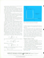
Download 1967 , Volume , Issue Sept-1967

HEWLETT-PACKARDJOURNAL
over: NEW NOISE GENERAT
RANDOM GAUSSIAN NOISE; page 2
SEPTEMBER 1967
© Copr. 1949-1998 Hewlett-Packard Co.
Pseudo-Random and Random Test Signals
Using digital techniques, this precision low-frequency
noise generator can synthesize repeatable, controllable,
pseudo-random noise patterns as well as truly random noise.
By George C. Anderson, Brian W. Finnic and Gordon T. Roberts
ALMOST EVERY NATURAL AND MAN-MADE SYSTEM ÃS
subject to random disturbances under normal oper
ating conditions. Consequently, it is often appropriate,
and sometimes essential, to test a system with random
test signals rather than with the sine waves that are so
familiar to electrical engineers.
Many of the areas of application for random test
signals lie outside the field of electrical engineering.
Examples are biomedical phenomena, vibration, aero
dynamics, and seismology. However, a growing number
of electrical problems fall into this same category.
For example, it is much more appropriate to test a
multi-channel telephone system with random noise sim
ulating each speech signal, than to use a number of sine
waves. The problem of communicating with deep space
probes is another subject that can be adequately treated
only by means of statistical techniques.
From the mathematical viewpoint, there
fore, there are good reasons for
using noise as a test signal. Yet,
despite the fact that adequate
theories have been developed,
the introduction of test methods
based on these theories has been
delayed by a lack of suitable,
convenient test equipment.
Chief among the many factors
responsible for this state of af
fairs is that conventional noise generators employ 'natu
ral' noise sources such as gas-discharge tubes and
temperature-limited diodes. The statistics of the noise
signals produced by these sources are not very stable,
well-defined, or controllable. The problem is most severe
at low audio and sub-audio frequencies, where much
of the current interest in noise testing is focused.
To circumvent these deficiencies, the development of
a new low-frequency noise generator was undertaken.
The result of this development program is the instrument
shown in Fig. 1. It is not a 'natural' noise source; it is a
precision noise generator which synthesizes noise and
noise-like (pseudo-random) signals by a controllable dig
ital process. As a result, the characteristics of its output
can be specified accurately and varied to fit the measure
ment situation.
This new measurement tool will realize its full potential
only after people understand it and begin to see how
they can use it to solve their problems. We hope to ac
celerate this process by describing how the new noise
generator works and some of the things it can do.
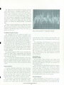
Fig. 1. A precision digital instrument. Model 3722A
Noise Generator synthesizes repeated pseudo-random noise-like
patterns or non-repealing random noise. Binary
(two-level) and Gaussian (multi-level) outputs are generated.
Amplitudes and bandwidths of outputs and lengths of
pseudo-random patterns are variable.
© Copr. 1949-1998 Hewlett-Packard Co.
Specifying Noise
How can noise be specified?
Simple deterministic signals can be completely speci
fied by a small number of parameters. For example, dc
is specified by only one parameter. A step function is
specified by two parameters — amplitude and time. And
a sine wave is specified by three parameters — amplitude,
frequency, and phase.
Random signals, on the other hand, can't be completely
specified by a finite number of parameters. But we still
need some way of describing them, so we resort to statis
tical descriptions which tell us about the average be
havior of the signals.
The simplest statistic of a noise signal is its meansquare value or, equivalently, its rms value. This param
eter is quite easy to measure, provided that we have an
instrument with a true square-law response. We also have
to carry out the averaging process over a long enough
time to reduce the statistical variance of the results to
an acceptably small value.
Power Density Spectrum
Another statistical description of a random signal that
isn't difficult to measure is its power density spectrum.
This tells us how the noise power contributed by separate
frequency components of the signal is distributed over
the frequency spectrum. It should have units of watts
per unit bandwidth, but it is common practice in noise
theory to consider (amplitude)- as the unit of power. For
electrical signals, this gives the power density spectrum
units of V2/Hz.
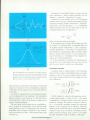
A power density spectrum is shown in Fig. 2. The
total area under this curve gives the total power con
tained in the signal. The power contributed by all fre
quency components in any band, say from f, to f2, is
equal to the area under the power density curve between
f, and f2 (shaded area in Fig. 2). Power density spectra
can be measured experimentally with a narrow-band,
constant-bandwidth wave analyzer followed by a true
square-law meter with a long averaging time.
* This inconsistency in the units of power is unacceptable to some engineers; they
reconcile the difficulty by assuming a one-ohm load resistance.
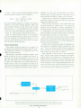
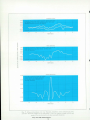
Model 180A Oscilloscope (bottom) displays
a portion of pseudo-random Gaussian noise pattern gen
erated by Model 3722A Noise Generator (center). Top
instrument is a display unit from new HP Model 5400A
Multi-channel Analyzer, which will be described in a
future issue of the Hewlett-Packard Journal. Here the
Analyzer displays the probability density function of the
noise generator's Gaussian output.
FREQUENCY (Hz)
Fig. 2. Typical power density spectrum for a random sig
nal. Total area under curve is mean-square value of signal,
usually spoken of as "power" in noise theory. Shaded area
is power in the frequency band f, to f:.
It is important to notice that the power density spec
trum is not the same as the power spectrum. The former
has units of V-'/Hz. The latter is just the square of the
amplitude spectrum and has units of V-. The power
spectrum is used to describe signals which have a finite
number of discrete frequency components. The ampli
tude or (amplitude)2 of each component can be repre
sented by a line of the proper length on the graph. But
when the signal is a complex random waveform, the
power spectrum has to have an infinite number of lines,
all of zero amplitude. Thus the power spectrum shrinks
to zero for a random signal. The power density spectrum,
however, does not disappear.
Noise which contains equal amounts of all frequencies
is called 'white' noise, by analogy to white light. White
noise has a power density spectrum which is simply a
horizontal line representing some non-zero value of
power per unit bandwidth. Truly white noise, which has
infinite bandwidth and therefore infinite power, is never
found in physical systems, which always have finite bandwidths. We usually call noise 'white' if it has a flat power
density spectrum over the band of interest.
Probability Density Functions
The power density spectrum tells us how the energy
of a signal is distributed in frequency. But it doesn't
specify the signal uniquely, nor does it tell us very much
about how the amplitude of the signal varies with time.
That the spectrum doesn't specify the signal uniquely
is a consequence of the fact that it contains no phase
information. Two periodic signals, for example, have the
same power spectrum if they both contain the same fre
quency components at the same amplitudes. But if the
© Copr. 1949-1998 Hewlett-Packard Co.
In general, the probability density function and the
power spectrum or power density spectrum are two
different — unrelated — properties of a signal.
Probably the most familiar pdf is the bell-shaped
Gaussian curve, Fig. 3(b), which is characteristic of many
naturally-occurring random disturbances. 'Gaussian'
means that a curve has the shape y = e'*2. Probability
density functions must all have areas equal to one, so
a Gaussian pdf must be normalized, i.e.,
p(x)=
Normalized
Probability
Density
«P M
Gaussian probability
density function
P(x) =
I
- X 2 / 2 " 2
it — rms value of x
2<r-
where a is the rms value of the signal.
It is important not to confuse the Gaussian pdf with
the output of a Gaussian filter. A Gaussian filter has
an impulse response shaped like e~x: and a frequency
response shaped like e~"\ The output of a Gaussian filter
may indeed have a Gaussian pdf. But an arbitrary signal
having a Gaussian pdf may have a power density spec
trum which bears no resemblance to the frequency re
sponse curve of the Gaussian filter.
It is also important to recognize that Gaussian noise
does not have to be white noise, and vice versa. The pdf
and the power density spectrum are independent.
Correlation Functions
(b)
Fig. 3. Probability density junction tells what proportion
of time is spent by signal at various amplitudes. Shaded
area in (a) is equal to proportion of lime spent hy signal
between x, and x,. Gaussian probability density junction
(b) is common to many natural disturbances.
phase of just one component of one signal is shifted with
respect to the phase of the corresponding component
of the other, the two signals can have drastically different
waveforms.
A statistic of a signal that gives waveshape information
and is independent of the spectrum is the probability
density function, or pdf (see Fig. 3). The pdf tells us
what proportion of time, on the average, is spent by the
signal at various amplitudes.
The area under a pdf between any two amplitudes x,
and Xj is equal to the proportion of time that the signal
spends between x, and x,. Equivalently, this area is the
probability that the signal's amplitude at any arbitrary
time will be between x: and x.. The total area under a pdf
is always one.
A statistic which is useful because it tells something
about the time or phase relationship between two signals
(random or not) is the cross-correlation between them.
The cross-correlation function for two signals x(t) and
y(t) is defined as
•T/2
R«(T)= lim -1 I x(t)y(t+r)dt
T-^oc T /-T/2
: lim —
T/2
x(t— r)y(t)dt.
-T/2
A block diagram of a system which performs this cal
culation approximately is shown in Fig. 4. One signal
is multiplied by a delayed version of the other and the
product is averaged. The result is a function of the de
lay T. In physically realizable systems the result also
depends on the averaging time T. Ideally T should be
infinite, but this would mean that it would take an infinite
amount of time to get an answer. Fortunately the sta
tistical variance caused by using a finite T can usually
be made acceptably small by making T fairly large.
© Copr. 1949-1998 Hewlett-Packard Co.
If y(t) = x(t) the cross-correlation function becomes
the autocorrelation function of x(t), defined as
T/2
X(t— r)x(t)dt.
-T/2
The autocorrelation function of a signal is the Fourier
transform of the power density spectrum. Hence the
autocorrelation function of white noise is just a single
delta-function at - = 0; this means that any two samples
of the same white noise signal are uncorrelated as long
as there is a nonzero time interval between them.
Since the autocorrelation function is the transform
of the power density spectrum, it gives us no information
that isn't contained in the spectrum. However, it is an
extremely useful function and is often simpler to compute
than the power density spectrum.
Pseudo-Random Noise
Noise makes a good test signal for two reasons: it is
broadband, and it realistically simulates naturally-occur
ring disturbances. However, its randomness is not very
helpful to the experimenter.
Theoretically, experiments involving random noise
should be carried out over an infinite time interval so
that only the average characteristics of the noise will
affect the result. But every real measurement can only
be made over a finite time, say T. This means that, if
random noise is used as a test signal, the result of an
experiment will, in general, be different from its expected
value. Or, if an experiment involving random noise is
repeated over and over, each repetition will yield a
different result. In other words, the randomness of the
noise introduces statistical variance into the results.
Variance can be reduced by extending the measure
ment time T. But it can never be made zero when truly
random test signals are used.
What we need, obviously, is a test signal which has
the good properties of random noise — i.e.. broad, flat
spectrum and resemblance to natural disturbances in
waveform and pdf — but doesn't have the bad property —
i.e., randomness. This signal should be one that intro
duces no statistical variance into the results, even though
the measurement is made over a finite time T.
Such a signal exists. Pseudo-random noise is a signal
which looks and acts like random noise, but is in fact
periodic. This kind of noise is one of the principal prod
ucts of the new noise generator.
Pseudo-random waveforms consist of completely de
fined patterns of selectable lengths, repeated over and
over*. They have spectra and pdf's that are similar to
those of random noise, but because they are synthesized,
their statistics are much easier to control.
Most important is the fact that if the measurement
time T is made exactly equal to the length of one pseudo
random pattern, the results of an experiment will be
identical on every repetition, as long as nothing else has
changed. There is no statistical variance. This means that
it isn't necessary to use a long measurement time, be
cause the reason for the long measurement time was to
* A good Simu on pseudo-random signals is G. A. Korn, 'Random Process Simu
lation 1966. Measurements,' New York, McGraw-Hill Book Company, 1966.
Approximate Correlation
Function
AVERAGING
CIRCUIT
*
T
Rxy(t) = j j X(t-T)y(t)dt
x(t) (Autocorrelation) or
y(t) (Cross-correlation)
Fig. signals. com functions show time relationships between signals. They can be com
puted by product. one signal by a delayed version of the other and averaging ¡he product.
© Copr. 1949-1998 Hewlett-Packard Co.
lOkii
100pF=b
Time Constant =
Time Constant = 10,'is
Part of 2047-Bit Pseudo Random
Binary Sequence. Clock Period =
3.33 ."S. Sweep Rate = 10 rs/cm.
lOkil
Time Constant = 200,»s
Fig. from pseudo-random or random Gaussian signals can be derived from pseudo-random
or random binary signals by low-pass filtering. To give good results, filter cutoff frequency
must be about 1/20 of clock frequency of binary signal.
reduce the variance introduced by random noise. Pseudo
random noise, therefore, can save a great deal of time.
The repeatability that pseudo-random noise gives an
experiment is especially valuable when parameters of
the system being tested are varied, as on an analog com
puter. In such tests, it is important to know that changes
in test results are caused by parameter manipulation and
not by statistical variance.
Because measurements using pseudo-random noise are
normally made over one pattern length, we lose none
of the advantages of random signals by substituting
pseudo-random signals, even though they are periodic.
Measurements using random noise must be made in a
finite time anyway, so it makes no difference whether the
signal repeats or not after the measurement time is over.
Binary and Gaussian Noise Generated
The most useful and most widely used pseudo-random
or random test signals are of two types — pseudo-random
or random binary (two-level) signals and pseudo-random
or random Gaussian (multi-level) signals. The Gaussian
signals are used in testing analog systems. The binary
© Copr. 1949-1998 Hewlett-Packard Co.
•
— — \T = Clock Period
_A_A_A_A_AJULA_A_A_A_A-A_
AT= Ins, 3.33MS, 10/<s
333s
NOTE: Scales on Spectrum Plots are Logarithmic.
BINARY
WAVEFORM
GENERATOR
Spectrum of Binary Output
-3dB at 0.45 fc
Ã- — - — j-Shaped Envelope
-o
Binary
Output
N = 2"-l. n =4. 5. 6, ••• ,20
N = 15. 31. 63. •••, 1048575.
or x
DIGITAL
LOW-PASS
FILTER
Cutoff
Frequency
= 1/20 Clock
//A
NAT NYT NT
|2_AT
FREQUENCY (Hz) / AT
-rf^— fc = Clock Frequency
Spectrum of Digital Filter Output
Filter Bandwidth Varies
I with Clock Frequency
-3dB
/ sin x 2
^- ( ' " (-Shaped Spectrun
' ' of Binary Signal
2 0
/
2 f c
3 f c
FREQUENCY (Hz) First Lobe of High-Frequency
Components in Digital Filter Output
ANALOG
SMOOTHING
FILTER
Spectrum of Gaussian Output
±0.3 dB at Vi f,
Corner Frequency of
Analog Smoothing Filter
"20
FREQUENCY (Hz)
Fig. or signal 3722 A Noise Generator synthesizes pseudo-random or random binary signal
in a digital waveform generator which is timed by a crystal-controlled clock. Clock rate
and length of pseudo-random sequences are variable. Gaussian signal is derived from bi
nary output by digital low-pass filtering. Discrete steps in digital filler output are removed
by analog filter. Pseudo-random binary output of noise generator has line power spectrum
having d flat envelope from dc to an upper 3 dB frequency which is selectable from 0.00135
Hz to 450 to Spectrum of pseudo-random Gaussian output has flat envelope from dc to
an upper 3 dB frequency which is selectable from 0.00015 Hz to 50 kHz. Random outputs
have envelopes power density spectra having same shapes as envelopes of spectra of
pseudo-random outputs.
© Copr. 1949-1998 Hewlett-Packard Co.
Fig. 7. Model 3722A NuÃ-se Generator produces sync pulse
(top), one clock period wide, at same point in each pseudo
random sequence.
The number N of clock periods in the pseudo-random
sequences is selectable from 2* — 1 to 220 — 1, i.e., from
15 to 1,048,575. The length of one sequence is the prod
uct of N and the clock period, so the number of seconds
in the pseudo-random sequences can be as short as 1 /-is
X 15 = 15 /¿s, or as long as 333 s X 1,048,575 = more
than 1 1 years!
When the SEQUENCE LENGTH switch is set to its
INFINITE position, the binary waveform generator is
primed by a solid-state random noise source. In this
condition, the binary signal is truly random and never
repeats.
As Fig. 6 shows, the binary signal is one of the outputs
from the noise generator. It is available at ±10 V with
very low impedance, or at a selected amplitude with 600
Q impedance. A relay-contact version of it is also avail
able if the selected clock period is greater than 100 ms.
Spectrum of the Binary Output
signals can be used in analog systems, in 'hybrid' sys
tems — e.g., a process control system containing solenoidoperated on-off valves — or in digital systems — e.g.,
a PCM channel.
Although binary and Gaussian noise look quite dif
ferent, it is possible to get a random Gaussian signal by
sending a random binary signal through a low-pass
filter (see Fig. 5).
The new noise generator produces both binary and
Gaussian pseudo-random and random outputs. Using
digital techniques, it synthesizes the binary waveform,
then low-pass-filters the binary signal to get the Gaussian
output.
Fig. 6 shows how the instrument works.
A binary waveform generator, timed by a crystalcontrolled clock, synthesizes the basic binary signal. The
changes of state of the binary signal always take place
when a clock pulse occurs, but a change doesn't occur
on every clock pulse. The clock period, and hence the in
terval between possible changes of state of the binary
signal, is selectable from 1 /¿s to 333 seconds. Alter
natively, the instrument may be timed by an external
clock of frequency up to 1 MHz.
Depending upon the setting of a front-panel SE
QUENCE LENGTH switch, the binary waveform gen
erator produces either repetitive or non-repetitive output
patterns. The repetitive, or pseudo-random patterns are
periodic, but they look random; there is apparently a
50% probability that the binary waveform will change
state on any given clock pulse. These waveforms repeat
after a fixed number, N, of clock periods.
A pseudo-random binary sequence has a line power
spectrum, the envelope of which is a (sin x/x)- curve, as
shown in Fig. 6. Note that most of the power is contained
in the first lobe, and that the nulls occur at intervals of
f,., the clock frequency. The harmonic (line) spacing is
a function of sequence length and clock frequency, and
is equal to f,./N or I/NAT where N is the number of bits
in the sequence and AT is the clock period.
The upper 3 dB (half-power) frequency of the binary
output is 0.45 f,.. Hence, by adjusting the clock period,
the operator can adjust the upper 3 dB frequency of the
binary signal from 0.00135 Hz to 450 kHz.
Regardless of what clock frequency (f,.) or sequence
length (N) is selected, the binary waveform always
switches between the same two amplitude levels. This
means that its rms value, and therefore its total power,
is not changed by a change of bandwidth. Halving the
bandwidth of the noise from a 'natural' noise source, on
the other hand, also halves the power; this is a disad
vantage when very low bandwidths are needed, since the
power available becomes very small.
The power density spectrum of the purely random
binary output (sequence length INFINITE) is continu
ous, i.e., it contains no discrete harmonics; it has the same
shape as the envelope of the pseudo-random power
spectrum.
Gaussian Output
The basic 'noise' produced by the noise generator is
a binary waveform having a nominal bandwidth (to the
half-power point) of 0.45 X clock frequency. While this
is noise in the sense that is contains a multiplicity of fre-
© Copr. 1949-1998 Hewlett-Packard Co.
quency components, it is a two-level waveform bearing
little resemblance — in the time domain — to naturally
occurring disturbances (thermal noise, atmospheric noise,
etc.). Naturally occurring noise can have a frequency
content similar to that of binary noise, but it is random in
amplitude, not confined to just two levels.
The noise generator provides, in addition to the basic
binary signal, pseudo-random or random signals of the
more familiar multi-level, or Gaussian type. 'Gaussian^
in this context, means that the probability density func
tion of the output tends to be the classical, bell-shaped
curve (see Fig. 3).
As we have shown (Fig. 5), a multi-level waveform
can be derived from a binary signal by conventional ana
log low-pass filtering. However, it takes a filter cutoff
frequency that is about 1/20 of the clock frequency to
give a reasonably Gaussian pdf. Since the lowest clock
frequency in the new noise generator is about one cycle
in five minutes, the lowest filter cutoff frequency has to
be about one cycle per 100 minutes! It simply isn't
practical to make analog filters with such low cutoff
frequencies.
To convert the output of the binary waveform gener
ator to a multi-level signal, we use a low-pass digital
filter which is not subject to the same limitations as a
conventional low-pass filter. The 3 dB bandwidth of the
filtered signal, defined as dc to the half-power frequency,
is nominally 1/20 of the clock frequency f,,.
The output of the digital filter is not a smooth signal,
but a series of steps, like any waveform that has been
generated digitally. These discrete steps in the multi-level
output of the digital filter are removed by low-pass analog
filtering (if the selected clock period is less than one
second), and the resulting smooth Gaussian signal is
another output of the noise generator. It is available at
a fixed amplitude of 3.16 V rms with low source imped
ance or at a selected amplitude with 600 O impedance.
Fig. 6 shows a typical Gaussian output waveform from
the noise generator, along with its spectrum. We will
have more to say about this signal when we discuss the
digital low-pass filter.
Control and Synchronization
Since pseudo-random signals are periodic, it is possible
to obtain a stationary display of them on an oscilloscope,
or to synchronize other equipment with them. For such
purposes, the noise generator produces a sync pulse, one
clock period wide, at a particular point in each pseudo
random sequence (Fig. 7).
Fig. 8. Fifteen-bit pseudo-random binary sequence is gen
erated by four stages of shift register with feedback.
Fig. 9. Fifteen-bit pseudo-random binary
sequence generated by system of Fig. 8.
Fig. 10. // n is number of stages involved in feedback loop,
length of pseudo-random sequence is N = 2" — / clock
periods. This is a 31-bit sequence generator, i.e., n = 5.
Besides the sync pulse, there is also a GATE output
which can be used for controlling external equipment
(e.g., a computer). Gate lengths of 1, 2, 4, or 8 pseudo
random sequences can be selected.
Another control feature is a HOLD button which,
when pressed, stops the pseudo-random waveform. Sub
sequently pressing the RUN button restarts the waveform
from the same point in the sequence that had been
reached when the HOLD button was pressed. There is
also a RESET button which sets the waveform gener
ator to the '0' state and removes its supply of clock
pulses. Pressing the RUN button then starts the gener
ator by restoring the clock pulses and placing a T in
the first stage of the waveform generator.
RUN, HOLD, and RESET can all be remotely pro
grammed.
© Copr. 1949-1998 Hewlett-Packard Co.
Shift-Register Waveform Generator
Many binary waveforms have the properties of pseudo
random sequences. One family, called maximal-length
sequences, can be generated by a shift register with ap
propriate feedback.
The binary waveform generator in the new noise
generator consists of the first 20 stages of a 32-stage
shift register. These 20 stages and the last 12 stages
also form part of the digital low-pass filter, which will
be discussed later. For now, we will concentrate on the
first 20 stages.
A shift-register stage is a special-purpose flip-flop. It
is an information store, and each stage of a shift register
can store one binary 'bit' of information ('0' or '!'). The
length of time that a bit of information remains in the
stage is equal to the time interval between two successive
clock, or shift, pulses.
Individual shift-register stages are connected in cas
cade so that, on receipt of shift pulses, the information
they contain is stepped progressively along the chain —
as if on a conveyor belt. (In this case, 'information' means
the pattern of ones and zeros in the register.)
The sequence generated by the four-stage arrange
ment of Fig. 8 can easily be derived. For the purpose of
illustration, the initial contents of the first four stages are
taken, arbitrarily, to be as follows:
Before 1st shift pulse
'0' waiting to go into stage (1)
on receipt of shift pulse
The modulo-two sum of the outputs from the last two
stages is '0' (this can be written 0 ® 0 = 0). At the first
shift pulse, the T in the first stage is transferred to the
second, and is replaced by the '0' in the feedback line.
This gives the pattern:
After 1st pulse
Pseudo-Random Sequence Generation
When generating pseudo-random binary sequences,
the shift register operates in a closed loop condition, and
the input to the first stage is supplied via a feedback path
from later stages of the shift register. Fig. 8 shows a
simple form of pseudo-random sequence generator. In
this example, only the first four of the shift-register stages
are actually involved in generation of the sequence.
Feedback to the first stage is taken from stages 3 and
4, the outputs from which are processed in an EXCLU
SIVE OR gate (otherwise known as: modulo-two adder,
half adder, non-equivalence or anti-coincidence gate).
This gate gives a T output only when its two inputs are
dissimilar, according to the following truth table:
Truth Table for EXCLUSIVE OR Gate
Again, the modulo-two summation yields '0! The next
pattern is therefore:
After 2nd pulse
With this pattern, the outputs from the third and fourth
stages are dissimilar — so the modulo-two sum is '1!
The T thus placed in the feedback line will enter the
first stage on arrival of the next shift pulse.
The remainder of the sequence can be worked out in a
similar manner. After the 14th pulse, the register pattern
is:
After 14th pulse
10
© Copr. 1949-1998 Hewlett-Packard
Co.
The fifteenth pulse restores the register to the initial state
(1000), and thereafter the sequence repeats.
With the exception of 0000, the register generates the
maximum number of T and '0' combinations possible
with four stages. The all-zero condition cannot arise (if
it were to occur, all stages of the shift register would
remain in the '0' state, and the output would thereafter
be an infinite sequence of zeros).
The pattern appearing at the output from the first
stage is exactly the same as that from the second, the
third and the fourth, and so on throughout the 32 stages
of the shift register. There is a delay of one clock period
between the pattern from one stage and the pattern from
the next. The digit sequence from any of the stages is:
Fig. 9 shows this sequence translated into a two-level,
or 'binary' waveform (T is represented by the relatively
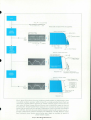
1. ANALOG FILTER
f t
y,(t) = h ( u ) x ( t - u ) d u
-'o
2. DELAY-LINE FILTER
y2(t) =
y2(t) = y,(t) if a, = h(j\T)
3. DIGITAL FILTER
Same x(t) signal Filter except delay line is shift register and x(t) is a binary signal
with clock period AT.
Fig. cutoff To get good Gaussian signals from binary signals, lowest cutoff frequency required
of low-pass filter in Model 3722A Noise Generator is about one cycle per 100 minutes.
This makes analog filter impractical, so generator uses digital approximation to ideal
low-pass filter. Delay line in noise generator is 32-stage shift register and weighting
networks a¡ are resistors.
© Copr. 1949-1998 Hewlett-Packard
Co.
11
~ RECIPROCAL
OF
RESISTANCE
rtional to Current Contribution
at Digital Filter Summing Point
7 8 91011121314151617181920212223242526:2728
Inverse
Outputs
of Flip-Flops
Outputs
of Flip-Flops
Fig. outputs For digital filter in Model 3722A Noise Generator, outputs of 32-stage flip-flop
shift register are weighted by resistors and added. Values of resistors are graded as shown
to make pulse response of filter approximate (sin x/x) shape.
negative level). This is the waveform obtained at the
BINARY connector of the noise generator with the
SEQUENCE LENGTH switch set to 15.
The next setting (31) of the SEQUENCE LENGTH
switch selects, for modulo-two addition, the outputs from
stages 3 and 5, as shown in Fig. 10. With five stages the
maximum number of T and '0' combinations is 32 but,
as before, the all-zero condition cannot occur. The result
ing sequence is therefore 31 bits long.
The number of stages included in the feedback loop
is increased by one at each setting of the SEQUENCE
LENGTH switch. Feedback is always taken from the
last of the 'active' stages, and from one or more of the
preceding stages. For the 127-bit sequence, for example,
feedback is taken from stage 7 (7 is the 'n' number en
graved on the front panel) and also from stages 3, 4,
and 5. Where more than two outputs are modulo-two
added, extra EXCLUSIVE OR gates are used.
The number of bits, N, in pseudo-random sequences
is always one less than the maximum number of T and
'0' combinations possible with the selected length of
register. Thus if n is the number of active stages, N =
2" — 1. In the new noise generator, n is variable from 4
to 20 and N ranges between 15 and 1,048,575.
1
Random Operation of the Shift Register
With the SEQUENCE LENGTH switch set to IN
FINITE, the feedback system is disconnected and the
first stage of the shift register is controlled by a semicon
ductor noise source, giving a truly random output signal.
Just before each shift pulse, the random signal is sampled
by a level detector which decides, on arrival of the shift
<
Fig. 13. Single-pulse response of digital filter is a discrete-step approxi
mation to (sin x/x)-shaped impulse response of ideal low-pass filler.
12
© Copr. 1949-1998 Hewlett-Packard
Co.
pulse, whether a T or a '0' is to be placed in the first
stage of the register. Since the random signal is nonperiodic, there is no repeated pattern in the resulting
series of ones and zeros from the register. The power
density spectrum of the random signal is continuous, and
has the same shape as the envelope of the power spectrum
of the pseudo-random signal.
Digital Low-pass Filter
A linear filter having an impulse response h(t) and
input x(t) has an output
/ h(u) x(t — u) du.
(1)
A finite-sum approximation to this integral can be
synthesized using a delay line. Fig. 1 1 shows a filter
composed of a delay line, a number of multipliers or
weighting networks, and a summing amplifier. The out
put of port j of the delay line is x(t — JAT) where x(t)
is the input and AT is the delay between ports. The sum
ming amplifier output is then
— JAT).
y(t) =
(2)
j==l
If 3j = h(jAT), and if n is sufficiently large, the sum,
equation 2, approximates the integral, equation 1.
When x(t) is a binary signal, as it is in the new noise
generator, the delay line can be a shift register. This in
fact is how the noise generator's digital low-pass filter
is constructed. It uses a 32-stage shift register as a delay
line. The first 20 stages of the same register do double
duty as the binary waveform generator, as we have
already explained.
The desired frequency response of the digital filter is
the rectangular response of an ideal low-pass filter. There
fore, the coefficients a.¡ are selected to approximate an
impulse response of (sin x/x) shape — the impulse re
sponse of an ideal low-pass filter.
)-Shaped Spectrum
of Binary Output
Frequency Characteristic of
Digital Low Pass Filter
First Lobe of H. F
Components
in Digital
Low- Pass
Filter Output
Fig. rectangular. Frequency response of digital low-pass filter is nearly rectangular. Small highfrequency components are caused by steps in digital-filter output; they are subsequently
removed by analog filtering.
13
© Copr. 1949-1998 Hewlett-Packard Co.
The weighting networks used in the noise generator
are simply resistors. The resistor values are chosen such
that the contributions of the outputs of successive shiftregister stages to the current at the summing point are
graded to follow the (sin x/x) curve, as shown in Fig. 12.
Notice in Fig. 12 that the contribution made by the
first and last groups of seven resistors is required to be
of the opposite polarity to that made by resistors in the
central group. This can be arranged by supplying all of
the weighting resistors in the central group with 'direct'
outputs from the shift register, and supplying those in
the outer groups with 'inverse' outputs ('direct' and
'inverse' are used here to describe the two outputs from
opposite sides of a flip-flop). AT starting at one end of
the register and being conveyed to the other, by a series
of shift pulses, will generate the time waveform shown
in Fig. 13.
George C. Anderson
^^^'^^(FT?
After graduating in 1954 from the
Heriot-Watt University (Edinburgh),
George Anderson completed a
two-year graduate apprenticeship
course in electrical engineering. This
was followed by varied industrial
work and a three-year period with
the Royal Observatory, where he
developed data recording systems
for the Seismology Unit. George, who
was the 3722A project leader,
joined HP in 1966.
Brian W. Finnic
Brian received the degree of BS from
Manchester University in 1962. He
spent the next three years at
Edinburgh University, where he
worked in the research team headed
by Gordon Roberts. He was
concerned with an advanced system
for real-time correlation, and was
awarded the degree of PhD for his
work in this field. Brian joined HP in
1965, and was responsible for initial
design work on the 3722A. He is
currently investigating a new range
of instrumentation, and is working
up routines for computer-aided
design using the HP 2116A.
Gordon T. Roberts
i
In 1954 Gordon graduated from the
University of Bangor (North Wales)
with the degree of BS in electrical
engineering. This was followed by a
three year period at Manchester
University, where he investigated
problems of noise in non-linear
systems; for this work, Gordon was
awarded the degree of PhD. After
five years of industrial work, a return
to more academic surroundings — this
time at Edinburgh University, where
he lectured in control theory and
headed a research team investigating
the uses of noise signals in systems
evaluation. Gordon has continued to
work in these fields since he joined
HP in 1965. He is now technical
manager of Hewlett-Packard Limited
in South Queensferry, Scotland.
Fig. 15. Bandwidth of ideal low-pass filler is inversely
proportional to time of first null in impulse response. In
noise generator, first null in digital-filter pulse response
occurs at nine clock periods, so cutoff frequency is theo
retically 1/18 of clock frequency. Actual response is not
ideal, and has 3 dB frequency equal to 1/20 of clock fre
quency. Thus bandwidth can be varied simply by changing
clock frequency.
14
© Copr. 1949-1998 Hewlett-Packard Co.
The digital filter has an effective frequency response
which approximates a rectangular spectrum (Fig. 14).
Owing to the limitation on the size of the shift register,
which results in truncation of the (sin x/x) curve, the
corner of the spectrum is not perfectly square. There are
also high-frequency components in the digital filter out
put spectrum. These components, caused by the abrupt
changes in output level as pulses pass down the shift
register, are removed by analog filtering, as described
later.
Changes in clock frequency do not affect the rectan
gular shape of the spectrum, they simply alter the upper
frequency limit. So here is a low-pass filter whose cut-off
frequency automatically keeps in step with clock fre
quency (see Fig. 15).
Fig. 16. Part of 8 191 -bit pscitdo-randuin (lausxian
pattern. Clock period is 1 ¡is; bandwidth is 50 kHz.
Probability Density Function
The amplitude pdf of the multi-level signal is not
significantly affected by the values of weighting resistor
assigned to the various stages. The Gaussian nature of
the pdf arises mainly from the apparent randomness of
the changing pattern of ones and zeros in the register —
the pdf becomes more nearly Gaussian as the sequence
length, and hence the 'randomness; is increased. This is
a consequence of the Central Limit Theorem of proba
bility theory, which states that the sum of a large number
of independent random variables tends to have a Gaus
sian pdf regardless of what the pdf's of the individual
variables look like.
For sequence lengths of 8191 or more, the pdf of the
multi-level signal closely approximates the Gaussian
curve, and the waveform closely resembles naturally
occurring noise (Fig. 16).
Fig. 17 shows the measured deviations of the noise
generator's output pdf from the true Gaussian curve for
sequence lengths of 8191 or greater. Worst-case devia
tions are less than ±0.020, which corresponds to about
±10%.
Analog Filtering
In analog computing applications, time derivatives
(i.e., differentiated versions) of signals occur frequently
and, whenever a signal has sharp edges, there is the dan
ger that derivatives could cause overload. In the case of a
boxcar waveform, with its very fast transit times, even
the first time derivative would be a series of very large
amplitude spikes, which could overload the system.
For this reason, a second-order analog filter is used
to remove sharp edges from the digital-filter output
waveform. As a result, neither the first nor the second
time derivatives of the waveform yield sharp spikes. The
pdf for both derivatives is reasonably Gaussian (see Fig.
17).
The analog filter cut-off frequency is selected by the
CLOCK PERIOD switch, and is nominally l/5th of the
clock frequency (that is, four times the half-power fre
quency of the digital filter). This feature is included for
all clock periods commonly of interest to analog com
puter users, i.e., noise bandwidth from 50 kHz to 0.15
Hz. At frequencies of 0.05 Hz and below, the analog
filter cut-off remains at the same frequency as for the
0.15 Hz position.
Crest Factor of
Gaussian Output
The crest factor (ratio of peak to rms values) of the
Gaussian output of the noise generator is 3.75, except
for the shortest sequences. This gives an excellent fit to
the Gaussian curve.
The crest factor of a truly Gaussian signal is, of course,
infinite, and some 'natural' noise sources have higher
crest factors than 3.75. However, it is often necessary
to wait a long time to be sure that one of their largest
peaks has occurred. With the pseudo-random output of
the noise generator, on the other hand, a definite number
of the highest peaks occur in every sequence.
Acknowledgments
Major contributions to the development of the noise
generator were made by Duncan Reid, Alistair Mac Parland, Glyn Harris, Michael Perry, and Richard Rex. •
15
© Copr. 1949-1998 Hewlett-Packard
Co.
GAUSSIAN OUTPUT
ENVELOPE (Shaded Area) SHOWS MEASURED DEPARTURES FROM
THE NORMAL CURVE OF 3722A GAUSSIAN OUTPUT PDF's FOR
SEQUENCE LENGTHS OF 8,191 AND GREATER
Sampling Window = 0.2
-3"
AMPLITUDE x
FIRST DERIVATIVE
MEASURED DEPARTURE FROM THE NORMAL C
FIRST DERIVATIVE OF GAUSSIAN SIGNAL OBTAINED WITH
32,767-BIT SEQUENCE
C
E
-3"
AMPLITUDE x
SECOND DERIVATIVE
-3.
AMPLITUDE x
Fig. density Measured deviations from true Gaussian probability density function for noise
generator 'Gaussian' output are less than about = W/c for sequence lengths of 8191 and
greater. First two derivatives are also reasonably Gaussian.
16 Co.
© Copr. 1949-1998 Hewlett-Packard
INTERNAL CLOCK
Crystal Frequency
3 MHz nominal.
SPECIFICATIONS
HP Model 3722A Noise Generator
Frequency Stability
<±25 ppm over ambient temperature range 0° to + 55°C.
BINARY OUTPUT (Fixed Amplitude)
Amplitude: MOV — 1 % when clock period >333 /is,
±3% when 1 ¿is < (clock period) <333 /is,
±5% when clock period = 1 jus.
Output
+ 1.5 V to +12.5 V rectangular wave, period as selected by CLOCK
PERIOD switch. Maximum current at 1.5 V level, 10 mA.
Output Impedance: <5 '..' if clock period >333 ,us,
< 10 !i if clock period <100 /is.
EXTERNAL CLOCK
Input Frequency
1 MHz maximum, for stated specifications. Usable BINARY output
(pseudo-random only) with external clock frequencies up to 1.5
MHz.
Load Impedance: 1kÃ-Ã- minimum.
Rise Time: <100 ns.
Power Density
Approxmately equal to (clock period x 200) WHz, at low frequency
end of spectrum.
Input Level
Negative-going signal from +5 V to +3 V initiates clock pulse.
Maximum input ±20 V.
Power Spectrum
(sin point form: first null occurs at clock frequency and -3 dB point
occurs at 0.45 x clock frequency.
Input Impedance: 1 k'..' nominal.
SECONDARY OUTPUTS
Sync
Negative-going pulse ( + 12.5 V to +1.5 V) occurring once per
pseudo-random sequence: duration of pulse equal to selected
clock period. Maximum current at 1.5 V level, 10 mA.
GAUSSIAN OUTPUT (Fixed Amplitude)
Amplitude: 3.16 V rms ±2% when bandwidth >0.15 Hz,
+ 6% -2% If bandwidth -'0.05 Hz.
This specification is valid only when sequence length >1,023.
Gate
Gate of indicates start and completion of selected number of
pseudo-random sequences (1, 2, 4 or 8, selected by front panel
control). Two outputs are provided:
1. Logic signal: output normally +12.5 V, falls to +1.5 V at
start of gate interval and returns to +12.5 V at end of
interval. Maximum current at 1.5 V level, 10 mA.
2. Relay changeover contacts: gate relay switching is syn
chronous with logic signal.
Maximum current controlled by relay: 500 mA (cont.).
Maximum voltage across relay contacts: 100 V.
Maximum load controlled by relay: 3 W (cont.).
Output Impedance: <1 '..
Load Impedance: 600 '..' minimum.
Zero Drift: <5 mV change in zero level in any 10°C range from 0° to
+ 55°C.
Power Density
Approximately equal to (clock period x 200) WHz at low frequency
end of spectrum.
Power Spectrum
Rectangular, low pass: nominal upper frequency f0 ( — 3 dB point)
equal to '^oth of clock frequency. Spectrum is flat within ±0.3 dB
up to 1/a f0, and more than 25 dB down at 2 f0.
Binary Relay
Relay changeover contacts operate In sync with binary output
signal (available only when clock period >100 ms). Relay speci
fication as for gate relay above.
Crest Factor: Up to 3.75, dependent on sequence length.
Probability Density Function: See error curves, page 16.
VARIABLE OUTPUT (Binary or Gaussian)
Amplitude (Open Circuit)
REMOTE CONTROL
Control Inputs
Remote control Inputs for RUN, HOLD, RESET and GATE RESET
functions are connected to 36-way receptacle on rear panel.
Command signal (each input): dc voltage between +1.5 V and
zero volts.
No-command condition: open-circuit input, or dc voltage between
+ 5.5 V and +12.5 V.
Input impedance: 5 k!; nominal (RUN, HOLD, RESET).
1.5 ki; nominal (GATE RESET).
BINARY
4 ranges: ±1 V, ±3 V, ±3.16 V and ±10 V, with ten steps in
each range, from X 0.1 to X 1.0.
GAUSSIAN
3 ranges: 1 V rms, 3 V rms and 3.16 V rms, with ten steps in each
range, from X 0.1 to X 1.0.
Calibration Accuracy
Better than ±2.5%, plus tolerance on binary or Gaussian output, as
selected.
Sequence Length Indication
18 pins plus one common pin on the 36-way receptacle are used
for remote signaling of selected sequence length (contact closure
between common pin and any one of the 18 pins).
Output Impedance: 600 !! ±1%.
MAIN CONTROLS
Sequence Length Switch
First 17 positions select different pseudo-random sequence lengths:
final position selects random mode of operation (INFINITE se
quence length). Sequence length (N) is number of clock periods
in sequence: possible values of N are 15, 31, 63, 127, 255, 511,
1023, 2047, 4095, 8191, 16383, 32767, 65535, 131071, 262143,
524287, 1048575. N = 2" — 1. where n is in the range 4 to 20
inclusive.
GENERAL
Construction: Standard 19 in. rack-width module, with tilt stand.
Ambient Temperature Range: 0° to +55°C.
Power Requirement: 115 or 230 V ±10%, 50 to 1000 Hz, 70 W.
Weight: Net 10.5 kg (23 Ib), shipping 13.5 kg (30 Ib).
Accessories Furnished
Detachable power cord, rack mounting kit, circuit extender board,
36-way male cable plug, operating and service manual.
CLOCK PERIOD SWITCH: Selects 18 frequencies from internal clock:
Price $2,650.00
OPTION 01
Zero Moment Option
Shifts relative position of sync pulse and pseudo-random binary
sequence such that first time moment of sequence, taken with
respect to sync pulse, is zero (sequence shift mechanism is oper
ative 01 when selected sequence length is <1023): option 01
also provides facility for inverting binary output signal.
ADD $50.00.
MANUFACTURING DIVISION: HEWLETT-PACKARD LTD.
South Queensferry
West Lothian, Scotland
17
© Copr. 1949-1998 Hewlett-Packard Co.
Testing with Pseudo- Random
and Random Noise
Pseudo-random noise is faster, more accurate, and more
versatile than random noise in most measurement situations.
process control system evaluation. Process control sys
tems can be tested for their responses to random
fluctuations in the controlled variables, e.g., tempera
ture, pressure, flow, concentration, etc. Pseudo-ran
dom signals are helpful here because they do not
introduce statistical variance into the results. Measure
ments are completed in the time required for only one
pseudo-random pattern. This is especially important
in low-speed systems, which might have to be tied up
for hours if truly random noise were used as a test
signal.
Pseudo-random noise is also especially useful in
testing large systems. As a system gets bigger, it gets
harder to test on a lab bench. Eventually it must be
tested under working conditions. A good example is an
airplane, which in the end must be tested in flight.
Pseudo-random noise can speed these tests for the
same reasons given above under 'process control sys
tem evaluation!
limited time situations. Pseudo-random noise is better
than random noise when the situation to be measured
exists only for a short time — e.g., a missile during
blastoff. Again, this is because measurements that use
pseudo-random noise are made over only one pattern
length, and no statistical variance is introduced into
the results by the noise.
THE NEW NOISE GENERATOR described in the article
beginning on page 2 is different from conventional
noise sources in that it synthesizes noise by a digital
process. This not only makes its output statistics more
stable and controllable, but also allows it to produce
pseudo-random noise as well as random noise. Pseudo
random signals are periodic signals that look random;
they have the same advantages as random noise for test
ing, but don't have the disadvantage of randomness.
Here are some of the ways in which noise is useful as
a test signal, with emphasis on the uses of pseudo-random
noise.
Noise as a Broadband Test Signal
Broadband noise makes an excellent test signal for
• environmental testing. For example, the vibrations
produced by a shake table with a noise input are
similar to those a product will meet in service. A loud
speaker connected to a noise generator makes a useful
acoustical noise source for testing microphones, mate
rials, rooms, and so on. In fatigue testing, pseudo
random noise is helpful because it has a known num
ber of peaks of various amplitudes; this means that
test time can often be reduced, since it is not necessary
to wait a long time to be sure a certain number of
peaks have occurred.
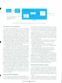
Accelerometer
HP 3722A
NOISE
GENERATOR
POWER
AMPLIFIER
18
© Copr. 1949-1998 Hewlett-Packard Co.
Fig. 1 . Model simulation
of tall structure.
Noise-driven shake
table simulates ground
disturbances, and
accelerometer measures
structure's response.
1 /-T
y / x(t-T)y(t)dt
J
x(t) is pseudo-random binary
output of HP 3722A.
Autocorrelation function RXX(T)
approximates an impulse.
See Figure 3.
CORRELATOR
Fig. correlation techniques. for obtaining impulse responses with noise and correlation techniques.
Flat Spectrum at Low Frequencies
In most of the applications of noise as a broadband
test signal, the preferred shape of the power density
spectrum is flat, at least through the band of interest.
This is a difficult requirement for conventional 'natural'
noise sources to meet, especially at low audio and subaudio frequencies, where flicker noise, 1/f noise, hum,
ambient temperature fluctuations, vibrations, and microphonics all degrade the spectrum. In addition, a noise
source usually produces a small amplitude signal. If low
frequencies are important, this signal must be amplified
by a dc coupled amplifier, and the random drifts of such
an amplifier cannot be distinguished from the low-fre
quency portion of the original noise signal.
Low-frequency noise, however, is a necessary product
of a useful noise source. The main use of very-low-fre
quency noise, e.g., in the 0 to 50 Hz range, is in testing
systems which have long time constants. These include
such things as massive mechanical arrays, nuclear re
actors, and chemical processes, where the effect of chang
ing any parameter of the process takes a long time to
become evident. When testing these systems, the lowest
frequency content of the test signal must be comparable
with the system time constant. This also holds true when
the system is being simulated on an analog computer.
The spectrum of the binary output of the new noise
generator is virtually flat from dc to an upper 3 dB fre
quency which can be adjusted from 0.00135 Hz to 450
kHz. The Gaussian signal has a spectrum which is flat
from dc to an upper 3 dB point of 0.00015 Hz to 50 kHz.
Regardless of selected cutoff frequency, the genera
tor's total power output is constant; in other words, when
we halve the bandwidth, we don't halve the power — as
occurs when the output from a conventional noise source
is low-pass filtered.
Model and Computer Simulation
Control systems, buildings, ships, automobiles, air
craft, aerospace guidance systems, bridges, missiles, and
a host of other complex objects can often be designed
and studied most easily by simulating them in the lab
oratory. This can be done either by using a scale model
of the object or by simulating it on an analog computer.
In either case, the new noise generator can provide
realistic simulations of road roughness, air turbulence,
earthquakes, storms at sea, target evasive action, controlled-variable fluctuations, and so on. Particularly use
ful is the pseudo-random output of the generator, which
has the same effect on the model as real noise, but which
can be repeated at will.
Analog computer users should find the following char
acteristics of the noise generator particularly helpful:
" accurately defined signals
• amplitude controls not subject to loading errors
« ability to change time scale without changing ampli
tude or pattern shape
• remote programming for RUN, HOLD, RESET
• gate circuits to control operations in the computer
« good autocorrelation function (see Fig. 3)
« zero-moment option (see Specifications, p. 17).
Fig. 1 shows a model simulation of a tall structure
mounted on a shake table which is being excited by
Gaussian noise from the new noise generator. This set-up,
currently in use at Edinburgh University, provides ex
perimental data on the behavior of tall buildings sub
jected to ground disturbances. The lower trace shows the
acceleration of the first floor of the structure, as measured
by the accelerometer mounted on the model.
Impulse Responses Without Impulses
All the information necessary to characterize a linear
system completely is contained in its impulse response.
Given any unknown system, then, it would be desirable
to be able to find its impulse response. One way to do
this would be to excite the system with an impulse or a
train of impulses and observe the output with an oscil
loscope.
However, impulses are dangerous; they are likely to
cause overload and saturation. Of course, small impulses
could be used, but if they are small enough to be safe they
19
© Copr. 1949-1998 Hewlett-Packard
Co.
usually produce outputs which are so small that they are
obscured by background disturbances.
One of the really interesting features of statistical tech
niques is that we can inject low-amplitude noise into a
system and, by suitably processing the output, obtain the
system impulse response, without subjecting the system
to a damaging high-level test signal. This technique has
two other advantages.
« The test may be performed while the system is operat
ing 'on line! This is possible because the intensity of
the noise test signal can be low enough so it doesn't
affect normal operation of the system.
» The results are largely unaffected by background dis
turbances in the system. This is because the results are
obtained by correlation, and the disturbances aren't
correlated with the test noise.
Fig. 2 shows a setup for obtaining impulse responses
from noise responses. The output of the system is crosscorrelated with the noise input; that is, the output is
multiplied by a delayed version of the input and the
product is averaged. The average as a function of the
delay T is the same as the impulse response of the system
as a function of time provided that the autocorrelation
junction of the noise input is an impulse (i.e., the noise
should be wideband compared with the system's fre
quency response). If the autocorrelation function of the
noise isn't a true impulse, the result will be less than
perfectly accurate. The accuracy of the correlator output
is also affected by the correlator's averaging time.
Mathematically, the setup of Fig. 2 works as follows.
If the noise is x(t), the unknown impulse response is h(t).
and the response of the system to the noise is y(t), then
00
•-f
y(t)= f h(u)x(t-u)du
— oo
The cross-correlation function of y(t) with x(t) is defined
3
5
/
-
T
/
2
lim ] ' x(t-r)y(t)dt.
—T/2
Substituting for y(t) gives
/«CO
/ h ( u ) R x (u — -)du.
J-oo
where Rxx(-) is the autocorrelation function of the noise
x(t). If Rxx(-) is a true impulse then
RX>(T) =
RxvM = ^ h(r),
where o-x is the rms value of the noise x(t). In other words,
N Clock Periods
(Length of Sequence)
= Mean-square value of
pseudo-random
binary signa
Fig. 3. Autocorrelation junction of pseudo-random
binary sequence approximates an impulse.
the unkown impulse response is proportional to the crosscorrelation function of the input noise x(t) with the
output y(t).
The binary pseudo-random noise synthesized by the
new noise generator has an autocorrelation function
which, while not precisely an impulse, is very close to
one, as shown in Fig. 3. What's more, the averaging
time T for the correlation system only needs to be as
long as one period of the pseudo-random waveform, i.e.,
as long as one complete pseudo-random pattern. Unlike
random noise, pseudo-random noise introduces no sta
tistical variance into the results, as long as the averaging
time T is exactly one pattern length.
Calibration, Research, Training
Other uses of the noise generator include
• research in communication, biomedical engineering
seismology, underwater sound, PCM, etc.
« calibration of true-rms voltmeters, spectrum analyzers,
and other low-frequency test equipment (e.g., the
pseudo-random signal generates a comb of frequencies,
useful for checking wave analyzers).
• student familiarization with random-signal theory and
the behavior of systems with noise inputs.
It will be interesting to see how this list grows as the
potential of controllable, repeatable noise becomes more
widely realized. •
HEWLETT-PACKARDJOURNAL¿S E P T E M B E R 1 9 6 7 V o l u m e 1 9 â € ¢ N u m b e r 1
TECHNICAL CALIFORNIA FROM THE LABORATORIES OF THE HEWLETT-PACKARD COMPANY PUBLISHED AT 1501 PAGE MILL ROAD PALO ALTO CALIFORNIA 94304
Editorial Stall F J BURKHAfÃ-D. R P DOLAN. L D SHERGALIS. R. H $NYD£R Art Director R A ERICKSON
© Copr. 1949-1998 Hewlett-Packard Co.