Download Bus Transit Capacity - Transportation Research Board

7UDQVLW&DSDFLW\DQG4XDOLW\RI6HUYLFH0DQXDO
PART 2
BUS TRANSIT CAPACITY
CONTENTS
1. BUS CAPACITY BASICS ....................................................................................... 2-1
Overview..................................................................................................................... 2-1
Definitions............................................................................................................... 2-1
Types of Bus Facilities and Service ............................................................................ 2-3
Factors Influencing Bus Capacity ............................................................................... 2-5
Vehicle Capacity ..................................................................................................... 2-5
Person Capacity..................................................................................................... 2-13
Fundamental Capacity Calculations .......................................................................... 2-15
Vehicle Capacity ................................................................................................... 2-15
Person Capacity..................................................................................................... 2-22
Planning Applications ............................................................................................... 2-23
2. OPERATING ISSUES............................................................................................ 2-25
Introduction............................................................................................................... 2-25
Bus Operations.......................................................................................................... 2-25
Passenger Loads.................................................................................................... 2-25
Skip-Stop Operation.............................................................................................. 2-26
Roadway Operations ................................................................................................. 2-28
Bus Preferential Treatments at Intersections ......................................................... 2-28
Bus Preferential Treatments on Roadway Segments ............................................. 2-33
Person Delay Considerations ................................................................................ 2-37
Roadway Operations Summary ............................................................................. 2-37
3. BUSWAYS AND FREEWAY HOV LANES........................................................ 2-39
Introduction............................................................................................................... 2-39
Calculating Vehicle Capacity.................................................................................... 2-40
Freeway HOV Lanes ............................................................................................. 2-40
Busways ................................................................................................................ 2-40
Calculating Person Capacity ..................................................................................... 2-41
Calculating Speed...................................................................................................... 2-42
4. EXCLUSIVE ARTERIAL STREET BUS LANES .............................................. 2-45
Introduction............................................................................................................... 2-45
Bus Lane Types......................................................................................................... 2-45
Calculating Vehicle Capacity.................................................................................... 2-47
Effects of Right Turns ........................................................................................... 2-47
Skip-Stop Adjustment Factor ................................................................................ 2-48
Vehicle Capacity ................................................................................................... 2-50
Bus Effects on Passenger Vehicle Capacity in an Adjacent Lane ......................... 2-52
Calculating Person Capacity ..................................................................................... 2-53
Calculating Speed...................................................................................................... 2-53
Base Bus Speeds ................................................................................................... 2-54
Right Turn Delays ................................................................................................. 2-54
Skip-Stop Operations ............................................................................................ 2-54
Bus-Bus Interference............................................................................................. 2-57
Part 2/BUS TRANSIT CAPACITY
Page 2-i
Contents
7UDQVLW&DSDFLW\DQG4XDOLW\RI6HUYLFH0DQXDO
5. MIXED TRAFFIC .................................................................................................. 2-59
Introduction ............................................................................................................... 2-59
Bus Lane Types......................................................................................................... 2-59
Calculating Vehicle Capacity .................................................................................... 2-60
Calculating Person Capacity...................................................................................... 2-61
Calculating Speed...................................................................................................... 2-62
6. DEMAND-RESPONSIVE ...................................................................................... 2-65
Introduction ............................................................................................................... 2-65
Vehicle Types........................................................................................................ 2-65
Operating Scenarios .............................................................................................. 2-66
Deviated Fixed-Route Transit ............................................................................... 2-66
Calculating Vehicle Capacity .................................................................................... 2-67
7. REFERENCES ........................................................................................................ 2-69
8. EXAMPLE PROBLEMS ....................................................................................... 2-71
APPENDIX A. DWELL TIME DATA COLLECTION PROCEDURE ................ 2-89
Introduction ............................................................................................................... 2-89
Passenger Service Times ........................................................................................... 2-89
Dwell Times .............................................................................................................. 2-90
APPENDIX B. EXHIBITS IN U.S. CUSTOMARY UNITS.................................... 2-93
LIST OF EXHIBITS
Exhibit 2-1 Examples of Freeway Vehicle and Person Capacity .................................... 2-2
Exhibit 2-2 Busway Examples ........................................................................................ 2-3
Exhibit 2-3 Exclusive Arterial Street Bus Lane Example (Portland, OR) ....................... 2-3
Exhibit 2-4 Mixed Traffic Example (Portland, OR)........................................................ 2-4
Exhibit 2-5 Typical Demand-Response Vehicle ............................................................. 2-4
Exhibit 2-6 Relationship Between Person and Vehicle Capacity .................................... 2-5
Exhibit 2-7 Bus Vehicle Capacity Factors ...................................................................... 2-6
Exhibit 2-8 On-Line and Off-Line Loading Areas .......................................................... 2-7
Exhibit 2-9 On-Street Bus Stop Locations .................................................................... 2-10
Exhibit 2-10 On-Street Bus Stop Location Comparison ............................................... 2-11
Exhibit 2-11 Person Capacity Factors ........................................................................... 2-13
Exhibit 2-12 Person Capacity Calculation Process ....................................................... 2-14
Exhibit 2-13 Typical Bus Passenger Boarding and Alighting Service Times for Selected
Bus Types and Door Configurations (Seconds per Passenger) ............................. 2-16
Exhibit 2-14 Average Bus Re-Entry Delay into Adjacent Traffic Stream (Random Vehicle
Arrivals) ................................................................................................................ 2-18
Exhibit 2-15 Values of Percent Failure Associated With Za.......................................... 2-19
Exhibit 2-16 Estimated Maximum Capacity of Loading Areas (Buses/h)..................... 2-20
Exhibit 2-17 Efficiency of Multiple Linear Loading Areas at Bus Stops...................... 2-20
Exhibit 2-18 Estimated Maximum Capacity of On-Line Linear Bus (bus/h) ................ 2-21
Exhibit 2-19 Bus Stop Maximum Vehicle Capacity Related to Dwell Times and Number
of Loading Areas................................................................................................... 2-21
Exhibit 2-20 Factors Influencing Bus Capacity............................................................. 2-23
Exhibit 2-21 Suggested Bus Flow Service Volumes for Planning Purposes (Flow Rates
For Exclusive or Near-Exclusive Lane) ................................................................ 2-24
Part 2/BUS TRANSIT CAPACITY
Page 2-ii
Contents
7UDQVLW&DSDFLW\DQG4XDOLW\RI6HUYLFH0DQXDO
Exhibit 2-22 Maximum Bus Passenger Service Volumes For Planning Purposes (Hourly
Flow Rates Based on 43 Seats Per Bus)................................................................ 2-24
Exhibit 2-23 Characteristics of Bus Transit Vehicles—United States and Canada....... 2-25
Exhibit 2-24 Example Skip-Stop Pattern and Bus Stop Signing ................................... 2-27
Exhibit 2-25 Bus Signal Priority Systems ..................................................................... 2-28
Exhibit 2-26 Bus Signal Priority Concept ..................................................................... 2-29
Exhibit 2-27 Bus Queue Jump Concept ........................................................................ 2-30
Exhibit 2-28 Bus Queue Jump Example (Copenhagen, Denmark) ............................... 2-30
Exhibit 2-29 Curb Extension Concept........................................................................... 2-31
Exhibit 2-30 Curb Extension Example (Vienna, Austria) ............................................. 2-31
Exhibit 2-31 Boarding Island Concept.......................................................................... 2-32
Exhibit 2-32 Boarding Island Example (San Francisco) ............................................... 2-32
Exhibit 2-33 General Planning Guidelines for Bus Priority Treatments—Arterials ..... 2-34
Exhibit 2-34 International Busway Examples ............................................................... 2-35
Exhibit 2-35 Freeway Ramp Queue Bypass Concept.................................................... 2-35
Exhibit 2-36 Freeway Ramp Queue Bypass Example (Los Angeles) ........................... 2-36
Exhibit 2-37 Typical Busway and HOV Lane Minimum Operating Thresholds
(veh/h/lane) ........................................................................................................... 2-36
Exhibit 2-38 General Planning Guidelines for Bus Priority Treatments—Freeways ... 2-37
Exhibit 2-39 Bus Preferential Treatments Comparison................................................. 2-38
Exhibit 2-40 Busway Examples .................................................................................... 2-39
Exhibit 2-41 Freeway HOV Lane Examples ................................................................. 2-39
Exhibit 2-42 Illustrative CBD Busway Capacities ........................................................ 2-41
Exhibit 2-43 Typical Busway Line-Haul Passenger Volumes....................................... 2-42
Exhibit 2-44 Estimated Average Speeds of Buses Operating in Freeway HOV Lanes
(km/h).................................................................................................................... 2-43
Exhibit 2-45 Type 1 Exclusive Bus Lane Examples ..................................................... 2-45
Exhibit 2-46 Type 2 Exclusive Bus Lane Examples ..................................................... 2-46
Exhibit 2-47 Type 3 Exclusive Bus Lane Examples ..................................................... 2-46
Exhibit 2-48 Bus Stop Location Factors, fl ................................................................... 2-48
Exhibit 2-49 Typical Values of Adjustment Factor, fk, for Availability of Adjacent Lanes
.............................................................................................................................. 2 -49
Exhibit 2-50 Values of Adjustment Factor, fk, for Type 2 Bus Lanes with Alternate TwoBlock Skip Stops................................................................................................... 2-49
Exhibit 2-51 Illustrative Exclusive Bus Lane Vehicle Capacity: Non-Skip Stop Operation
.............................................................................................................................. 2-51
Exhibit 2-52 Illustrative Exclusive Bus Lane Vehicle Capacity: Skip-Stop Operation. 2-51
Exhibit 2-53 Estimated Arterial Street Bus Speeds, V0 (km/h) ..................................... 2-55
Exhibit 2-54 Illustrative Skip-Stop Speed Adjustment Effects ..................................... 2-56
Exhibit 2-55 Bus-Bus Interference Factor, fb ................................................................ 2-57
Exhibit 2-56 Illustrative Bus-Bus Interference Factor Effects ...................................... 2-57
Exhibit 2-57 Type 1 Mixed Traffic Bus Lane (Portland, OR) ...................................... 2-59
Exhibit 2-58 Type 2 Mixed Traffic Bus Lane (Vancouver, BC)................................... 2-60
Exhibit 2-59 Illustrative Mixed Traffic Maximum Bus Vehicle Capacity .................... 2-61
Exhibit 2-60 Estimated Bus Speeds, V0 (km/h)—Mixed Traffic................................... 2-63
Exhibit 2-61 Characteristics of Different Demand-Responsive Bus Systems ............... 2-65
Exhibit 2-62 Demand-Responsive Transit Service Patterns.......................................... 2-66
Exhibit 2-63 Deviated Fixed-Route Service Patterns.................................................... 2-67
Exhibit 2-64 Sample Passenger Service Time Data Collection Sheet........................... 2-90
Exhibit 2-65 Sample Dwell Time Data Collection Sheet .............................................. 2-91
Part 2/BUS TRANSIT CAPACITY
Page 2-iii
Contents
7UDQVLW&DSDFLW\DQG4XDOLW\RI6HUYLFH0DQXDO
This page intentionally blank.
Part 2/BUS TRANSIT CAPACITY
Page 2-iv
Contents
7UDQVLW&DSDFLW\DQG4XDOLW\RI6HUYLFH0DQXDO
1. BUS CAPACITY BASICS
OVERVIEW
Bus capacity is a complex topic: it deals with the movement of both people and
vehicles, depends on the size of the buses used and how often they operate, and reflects
the interaction between passenger traffic concentrations and vehicle flow. It also depends
on the operating policy of the service provider, which normally specifies service
frequencies and allowable passenger loadings. Ultimately, the capacities of bus routes,
bus lanes, and bus terminals, in terms of persons carried, are generally limited by (1) the
ability of stops or loading areas to pick up and discharge passengers, (2) the number of
vehicles operated, and (3) the distribution of boardings and alightings along a route.
Bus capacity is complex,
incorporating a number of factors.
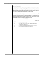
Part 2 of the Transit Capacity and Quality of Service Manual presents methods for
calculating bus capacity and speed for a variety of facility and operating types.
Organization of Part 2.
•
Chapter 1 introduces the basic factors and concepts that determine bus capacity.
•
Chapter 2 discusses bus and roadway operating issues that influence bus
capacity.
•
Chapters 3-6 present capacity and speed calculation procedures for four facility
and operating categories. The Types of Bus Facilities and Service section below
discusses these categories in further detail.
•
Chapter 7 contains references for material presented in Part 2 which may be
consulted for further information on how the procedures were developed.
•
Chapter 8 presents example problems that illustrate how to apply the procedures
introduced in Part 2 to “real world” situations.
•
Appendix A provides a procedure for collecting bus dwell time data in the field.
•
Appendix B provides substitute exhibits in U.S. customary units for Part 2
exhibits that use metric units.
Passenger service times at major
bus stops, and the number of
vehicles operated, usually
determine bus route and lane
person capacity.
Exhibits also appearing in
Appendix B are indicated by a
marginal note such as this.
Definitions
Throughout Part 2, the distinction is made between vehicle and person capacity.
Vehicle capacity reflects the number of buses that can be served by a loading area, bus
stop, bus lane, or bus route during a specified period of time. Person capacity reflects the
number of people that can be carried past a given location during a given time period
under specified operating conditions without unreasonable delay, hazard, or restriction,
and with reasonable certainty.
Vehicle vs. person capacity.
This definition of person capacity is less absolute than definitions of vehicle capacity,
because it depends on the allowable passenger loading set by operator policy and the
number of buses operated. Because the length of time that passengers remain on a bus
affects the total number of passengers that may be carried over the entire length of a
route, person capacity is often measured at a route’s maximum load point. For example,
an express bus may have most of its passengers board in a suburb and disembark in the
CBD. In this situation, the number of passengers carried at the maximum load point will
be close to the total number of boarding passengers. For a local bus, with a variety of
potential passenger trip generators along the length of the route, the number of persons
carried over the length of the route will be significantly greater than the express bus,
although both bus’ passenger loads at their respective maximum load points may be quite
similar.
As the length of time that
passengers remain on a bus
affects how many passengers
may be carried over the length of
a route, person capacity is often
measured at a route’s maximum
load point, rather than measured
for the route as a whole.
Part 2/BUS TRANSIT CAPACITY
Page 2-1
Chapter 1—Bus Capacity Basics
7UDQVLW&DSDFLW\DQG4XDOLW\RI6HUYLFH0DQXDO
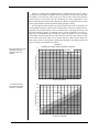
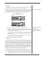
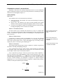
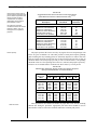
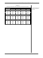
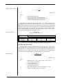
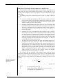
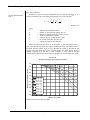
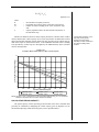
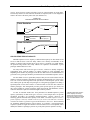
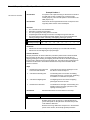
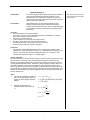
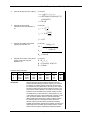
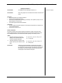
Exhibit 2-1 illustrates the relationship between vehicle and person capacity, using a
freeway lane as an example. The number of buses operated is set by the service provider.
The number of cars that can operate in the lane used by buses reflects the passenger
vehicle capacity of the freeway lane after deducting the vehicle equivalencies of the
buses. The total person capacity thus represents the number of people that can be carried
by the specified number of buses and the remaining passenger vehicles.
For the purposes of this example, the capacity of the freeway lanes are assumed to be
2,300 passenger vehicles per hour per lane (without buses), one bus is assumed to be the
equivalent of 2 passenger vehicles, buses are assumed not to stop along the freeway, and
buses and passenger vehicles are assumed to have average occupancies of 47 and 1.3,
respectively, corresponding to typical major-city vehicle occupancies. It can be seen that
as the number of buses using a freeway lane increases to 300, the person capacity of that
lane increases from about 3,000 to over 16,800, while the vehicle capacity drops only
from 2,300 to 2,000 (1,700 passenger vehicles plus 300 buses). Note that this figure only
refers to capacity, not to demand or actual use.
Exhibit 2-1
Examples of Freeway Vehicle and Person Capacity
Buses generally form a small
percentage of the total
vehicular volume on a
roadway…
2500
Total Vehicles
2250
Vehicles Per Lane Per Hour
2000
1750
1500
Cars
1250
1000
750
500
250
Buses
0
0
25
50
75
100
125
150
175
200
225
250
275
300
225
250
275
300
Buses Per Hour (No Stops)
18000
…but have the ability to
carry most of the people
traveling on a roadway.
16000
People per Lane per Hour
14000
Total People
12000
10000
Cars
8000
6000
Buses
4000
2000
0
0
25
50
75
100
125
150
175
200
Buses Per Hour (No Stops)
Part 2/BUS TRANSIT CAPACITY
Page 2-2
Chapter 1—Bus Capacity Basics
7UDQVLW&DSDFLW\DQG4XDOLW\RI6HUYLFH0DQXDO
TYPES OF BUS FACILITIES AND SERVICE
The capacity procedures presented in Part 2 categorize bus service by the kinds of
facilities that buses operate on, and, in the case of demand-responsive service, by the
special operating characteristics that influence capacity. These procedures will be
presented in order from the most exclusive kinds of facilities used by buses to the least
exclusive.
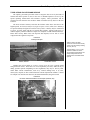
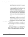
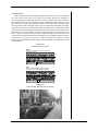
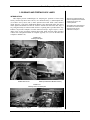
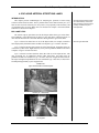
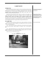
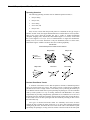
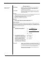
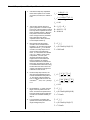
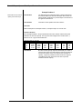
The most exclusive facilities, and often the facilities where buses can achieve the
highest speeds, are busways and freeway high-occupancy vehicle (HOV) lanes. Busways
are special roadways designed for exclusive use by buses. A busway may be constructed
at, above, or below grade and may be located either within a separate right-of-way or
within a highway corridor. Exhibit 2-2 depicts two examples of North American busways.
Buses share freeway HOV lanes with carpools and vanpools, but are able to avoid
congestion in the regular freeway lanes.
Exhibit 2-2
Busway Examples
Ottawa, Ontario has North
America’s most extensive busway
system, with five busways totaling
32.2 km (19.3 mi).
The five-station, 2.1-km (1.3-mi)
downtown Seattle bus tunnel
serves dual-powered (electric and
diesel) trolleybuses and was
designed to accommodate future
light rail.
Ottawa, Ontario
Seattle Bus Tunnel
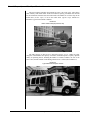
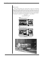
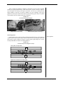
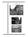
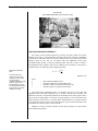
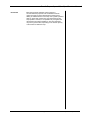
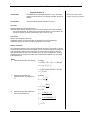
Another form of bus facility is exclusive arterial street bus lanes, typically found
along downtown streets. These lanes are reserved primarily for buses, either all day or
during specified periods. Depending on local regulations, they may be used by other
traffic under certain circumstances, such as by vehicles making turns, or by taxis,
motorcycles, carpools, or other vehicles that meet certain requirements. Exhibit 2-3 shows
an example of an arterial street bus lane, the downtown Portland, Oregon bus mall.
Exhibit 2-3
Exclusive Arterial Street Bus Lane Example (Portland, OR)
Part 2/BUS TRANSIT CAPACITY
Page 2-3
Chapter 1—Bus Capacity Basics
7UDQVLW&DSDFLW\DQG4XDOLW\RI6HUYLFH0DQXDO
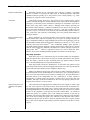
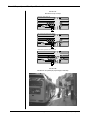
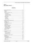
The most common operating environment for buses is in mixed traffic, where buses
share roadways with other traffic. In this environment, capacity procedures must account
for the interactions between buses and other traffic and whether or not buses stop in the
traffic lanes (on-line stops) or out of the traffic lanes (off-line stops). Exhibit 2-4
illustrates a typical mixed-traffic condition.
Exhibit 2-4
Mixed Traffic Example (Portland, OR)
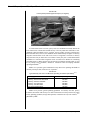
The final category of bus service is demand-responsive service. Unlike the other
categories, which address the capacity of facilities, demand-responsive capacity depends
mostly on operating factors, including the number of vehicles available, the size of the
service area, and the amount of time during which service is offered (See Exhibit 2-5).
Exhibit 2-5
Typical Demand-Response Vehicle
Part 2/BUS TRANSIT CAPACITY
Page 2-4
Chapter 1—Bus Capacity Basics
7UDQVLW&DSDFLW\DQG4XDOLW\RI6HUYLFH0DQXDO
FACTORS INFLUENCING BUS CAPACITY
This section presents the primary factors that determine bus vehicle and person
capacity. These concepts will be used throughout the remainder of Part 2. Although many
of the individual factors influencing vehicle capacity are different than those influencing
person capacity, this section will show that there are strong connections between vehicle
and person capacity, as well as between capacity in general and the concept of quality of
service introduced in Part 5.
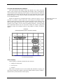
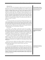
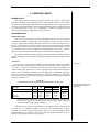
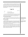
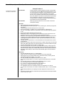
Exhibit 2-6 illustrates the two-dimensional nature of urban bus capacity. It can be
seen that it is possible to operate many buses, each carrying few passengers. From a
highway capacity perspective, the number of vehicles could be at or near capacity, even if
they run nearly empty. Alternatively, few vehicles could operate, each overcrowded. This
represents a poor quality of service from the passenger perspective, and long waiting
times would further detract from user convenience. Finally, the domain of peak-period
operations in large cities commonly involves a large number of vehicles, each heavily
loaded.
Relationship of person and
vehicle capacity.
Exhibit 2-6
Relationship Between Person and Vehicle Capacity
CRUSH LOAD (MAXIMUM PEOPLE PER VEHICLE)
CROWDED VEHICLES
FEW VEHICLES
E
MAXIMUM DESIGN LOAD (PEAK)
DOMAIN OF PEAK
PERIOD
OPERATIONS
D
C
MANY VEHICLES
FEW
PASSENGERS
B
MAXIMUM VEHICLES PER CHANNEL PER HOUR
Level of Service--Passenger (area/passenger)
F
A
A
B
C
D
E
F
Level of Service--Bus (vehicles/hour)
Vehicle Capacity
Vehicle capacity is commonly calculated for three locations:
•
loading areas (bus berths);
•
bus stops; and
•
bus lanes.
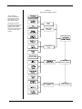
Each of these locations has one or more elements that determines its capacity, and
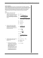
each of these elements has a number of factors that further influence capacity. Exhibit 2-7
illustrates the key factors that affect vehicle capacity.
Part 2/BUS TRANSIT CAPACITY
Page 2-5
Chapter 1—Bus Capacity Basics
7UDQVLW&DSDFLW\DQG4XDOLW\RI6HUYLFH0DQXDO
Exhibit 2-7
Bus Vehicle Capacity Factors
Vehicle capacity is
commonly calculated at
three locations: loading
areas (bus berths), bus
stops, and bus lanes.
Dwell
Time
The capacity of each of
these locations is influenced
by one or more elements
(middle column), each of
which in turn is influenced by
a number of factors (left
column).
Dwell Time
Variability
Clearance
Time
Bus Queuing
("Failure Rate")
Part 2/BUS TRANSIT CAPACITY
Page 2-6
Number of
Loading Areas
Bus Stop
Vehicle Capacity
Bus Operational
Issues
Bus Lane
Vehicle Capacity
Chapter 1—Bus Capacity Basics
7UDQVLW&DSDFLW\DQG4XDOLW\RI6HUYLFH0DQXDO
Loading Areas
A loading area, or bus berth, is a space for buses to stop and board and discharge
passengers. Bus stops, discussed below, contain one or more loading areas.
The most common form of loading area is a linear bus stop along a street curb. In this
case, loading areas can be provided in the travel lane (on-line), where following buses
may not pass the stopped bus, or out of the travel lane (off-line), where following buses
may pass stopped vehicles. Exhibit 2-8 depicts these two types of loading areas.
On-line vs. off-line loading areas.
Exhibit 2-8
(R6)
On-Line and Off-Line Loading Areas
On-Line
BUS
Off-Line
BUS
Elements affecting loading area
vehicle capacity.
The main elements affecting loading area vehicle capacity are the following:
•
Dwell Time. Dwell time is the single most important factor affecting vehicle
capacity. It is the time required to serve passengers at the busiest door, plus the
time required to open and close the doors.
•
Dwell Time Variability. The variations in dwell time among different buses using
the same loading area affect capacity. The greater the variation, the lower the
vehicle capacity.
•
Clearance Time. Clearance time is the average time between one bus leaving a
stop and a following bus being able to enter the stop.
Dwell time is the single most
important factor affecting vehicle
capacity.
Each of these elements is addressed in more detail below.
Dwell Time
Just as dwell times are key to determining vehicle capacity, passenger demand
volumes and passenger service times are key to determining dwell time. Dwell times may
be governed by boarding demand (e.g., in the p.m. peak period when relatively empty
buses arrive at a heavily used stop), by alighting demand (e.g., in the a.m. peak period at
the same location), or by total interchanging passenger demand (e.g., at a major transfer
point on the system). In all cases, dwell time is proportional to the boarding and/or
alighting volumes times the service time per passenger. Dwell time can also influence a
bus operator’s bottom line: if average bus speeds can be increased by reducing dwell
time, fewer vehicles may be required to provide the same service frequency on a route, if
the cumulative change in dwell time exceeds the existing route headway.
As shown in Exhibit 2-7, there are five main factors that influence dwell time. Two of
these relate to passenger demand, while the other three relate to passenger service times:
•
Passenger Demand and Loading. The number of people boarding and/or
alighting through the highest-volume door is the key factor in how long it will
Part 2/BUS TRANSIT CAPACITY
Page 2-7
Chapter 1—Bus Capacity Basics
7UDQVLW&DSDFLW\DQG4XDOLW\RI6HUYLFH0DQXDO
take for all passengers to be served. If standees are present on-board a bus as it
arrives at a stop, or if all seats become filled as passengers board, service times
will be higher than normal because of congestion in the bus aisleway. The mix of
alighting and boarding passengers at a stop also influences how long it takes all
passenger movements to occur.
Wheelchair and bicycle
boarding times may also
need to be considered when
calculating dwell time.
•
Bus Stop Spacing. The fewer the stops, the greater the number of passengers
who will need to board at a given stop. A balance is required between too few
stops (which increase the distance riders must walk to access transit and increase
the amount of time an individual bus occupies a stop) and too many stops (which
reduce overall travel speeds due to the time lost in accelerating, decelerating,
and possibly waiting for a traffic signal every time a stop is made).
•
Fare Payment Procedures. The amount of time passengers must spend paying
fares is a major factor in the total time required per boarding passenger. This
time can be reduced by minimizing the number of bills and coins required to pay
a fare; encouraging the use of pre-paid tickets, tokens, passes, or smart cards;
using a proof-of-payment fare-collection system; or developing an enclosed,
monitored paid-fare area at high-volume stops. In addition to eliminating the
time required for each passenger to pay a fare on-board the bus, proof-ofpayment fare collection systems also allow boarding passenger demand to be
more evenly distributed between doors, rather than being concentrated at the
front door.
•
Vehicle Types. Low-floor buses decrease passenger service time by eliminating
the need to ascend and descend steps. This is particularly true when a route is
frequently used by the elderly, persons with disabilities, or persons with strollers
or bulky carry-on items.
•
On-Board Circulation. Encouraging people to exit via the rear door(s) on buses
with more than one door decreases passenger congestion at the front door and
reduces passenger service times.
In certain locations, dwell time can also be affected by the time to board and
disembark passengers in wheelchairs, and for bicyclists to load and unload bicycles onto a
bus-mounted bicycle rack.
Combinations of these factors can substantially reduce dwell times. Denver’s 16th
Street Mall shuttle operation is able to maintain 75-second peak headways with scheduled
12.5-second dwell times, despite high peak passenger loads on its 70-passenger buses.1
This is accomplished through a combination of fare-free service, few seats (passenger
travel distances are short), low-floor buses, and three double-stream doors on the buses.
Dwell Time Variability
Not all buses stop for the same amount of time at a stop, depending on fluctuations in
passenger demand between buses and between routes. The effect of variability in bus
dwell times on bus capacity is reflected by the coefficient of variation of dwell times,
which is the standard deviation of dwell time observations divided by the mean dwell
time. Dwell time variability is influenced by the same factors that influence dwell time.
1
Denver’s Regional Transit District (RTD) planned to switch to 128-passenger buses in 1999 to accommodate
growing passenger demand for this service.
Part 2/BUS TRANSIT CAPACITY
Page 2-8
Chapter 1—Bus Capacity Basics
7UDQVLW&DSDFLW\DQG4XDOLW\RI6HUYLFH0DQXDO
Clearance Time
Once a bus closes its doors and prepares to depart a stop, there is a period of time,
known as the clearance time, during which the loading area is not available for use by the
following bus. Part of this time is fixed, consisting of the time for a bus to start up and
travel its own length, clearing the stop. For on-line stops, though, this is the only
component of clearance time. For off-line stops, however, there is another component to
clearance time: the time required for a suitable gap in traffic to allow the bus to re-enter
the traffic stream and accelerate. This re-entry delay is variable and depends on the traffic
volume in the travel lane adjacent to the stop and increases as traffic volumes increase.
The delay also depends on the platooning effect from upstream traffic signals. Some
states have passed laws requiring motorists to yield to buses re-entering a roadway;
depending on how well motorists comply with these laws, the re-entry delay can be
reduced or even eliminated. Many bus operators avoid using off-line stops on busy streets
in order to avoid this re-entry delay.
The time required for a bus to
start up and travel its own length
is fixed; re-entry delay for off-line
stops is dependent on traffic
volumes in the curb lane.
Bus Stops
A bus stop is an area where one or more buses load and unload passengers. It consists
of one or more loading areas. Bus stop vehicle capacity is related to the vehicle capacity
of the individual loading areas at the stop, the bus stop design, and the number of loading
areas provided. Off-line bus stops provide greater vehicle capacity than do on-line stops
for a given number of loading areas, but in mixed-traffic situations, bus speeds may be
reduced if heavy traffic volumes delay buses exiting a stop. The design of off-street bus
terminals and transfer centers entails additional considerations.
Bus Terminals
The design of a bus terminal or “transit center” involves not only estimates of
passenger service times of buses that will use the center, but also a clear understanding of
how each bus route will operate. Therefore, such factors as schedule recovery times,
driver relief times, and layovers to meet scheduled departure times become the key factors
in establishing loading area requirements and sizing the facility. In addition, good
operating practice suggests that each bus route, or geographically compatible groups of
routes, should have a separate loading position to provide clarity for passengers.
Bus stop design for bus terminals
must consider passenger factors
and take into account longer
loading area occupancies by
buses.
Loading area space requirements should recognize the specific type of transit
operations, fare collection practices, bus door configurations, passenger arrival patterns,
amount of baggage, driver layover-recovery times, terminal design, and loading area
configuration. They should reflect both scheduled and actual peak period bus arrivals and
departures, since intercity bus services regularly run “extras” during the busiest seasonal
travel periods.
Bus route and service patterns also influence loading area requirements. Good
operating practice calls for a maximum of two distinct routes (i.e., “services”) per loading
position. Part 4 of this manual describes sizing bus terminals in greater detail.
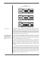
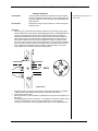
On-Street Bus Stops
On-street bus stops are typically located curbside in one of three locations: (1) nearside, where the bus stops immediately prior to an intersection, (2) far-side, where the bus
stops immediately after an intersection, and (3) mid-block, where the bus stops in the
middle of the block between intersections. Under certain circumstances, such as when
buses share a stop with streetcars running in the center of the street, or when exclusive bus
lanes are located in the center of the street, a bus stop may be located on a boarding island
within the street rather than curbside. When boarding islands are used, pedestrian safety
and ADA accessibility issues should be carefully considered. Exhibit 2-9 depicts typical
on-street bus stop locations.
Part 2/BUS TRANSIT CAPACITY
Page 2-9
The three typical on-street bus
stop locations are near-side, farside, and mid-block.
Chapter 1—Bus Capacity Basics
7UDQVLW&DSDFLW\DQG4XDOLW\RI6HUYLFH0DQXDO
Exhibit 2-9
(R6)
On-Street Bus Stop Locations
Near-Side
BUS
Far-Side
BUS
Mid-Block
BUS
Freeway bus stops.
Special bus stops are sometimes located along freeway rights-of-way, usually at
interchanges or on parallel frontage roads. Examples include stops in Marin County,
California and in Seattle, where they are known as “flyer stops.” These stops are used to
reduce travel time for buses by eliminating delays associated with exiting and re-entering
freeways. Freeway stops should be located away from the main travel lanes and adequate
acceleration and deceleration lanes should be provided. To be successful, attractive, welldesigned pedestrian access to the stop is essential.(R5)
Far-side stops have the
most beneficial effect on bus
stop vehicle capacity, but
other factors must also be
considered when siting bus
stops
The bus stop location influences vehicle capacity, particularly when passenger
vehicles are allowed to make right turns from the curb lane (as is the case in most
situations, except for certain kinds of exclusive bus lanes). Far-side stops have the least
effect on capacity (when buses are able to use an adjacent lane to avoid right-turn
queues), followed by mid-block stops, and near-side stops.
However, vehicle capacity is not the only factor which must be considered when
selecting a bus stop location. Potential conflicts with other vehicles operating on the
street, transfer opportunities, the distances passengers must walk to and from the bus stop,
locations of passenger generators, signal timing, driveway locations, physical
obstructions, and the potential for implementing transit preferential measures must also be
considered.
For example, near-side stops are preferable when curb parking is allowed, since there
is more space for buses to re-enter the moving traffic lane. They are also desirable at
intersections where buses make a right turn and at intersections with one-way streets
moving from right to left. Where buses operate in the curb lane and/or right-turning traffic
is heavy, far-side stops are preferable. Far-side stops are also used at intersections where
buses make left turns and at intersections with one-way streets moving from left to right.
Mid-block stops are typically only used at major passenger generators or where
insufficient space exists at adjacent intersections.(R5)
Part 2/BUS TRANSIT CAPACITY
Page 2-10
Chapter 1—Bus Capacity Basics
7UDQVLW&DSDFLW\DQG4XDOLW\RI6HUYLFH0DQXDO
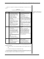
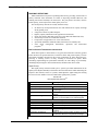
Exhibit 2-10 compares the advantages and disadvantages of each kind of bus stop
location.
Exhibit 2-10
(R6)
On-Street Bus Stop Location Comparison
Location
Far-Side
Advantages
• Minimizes conflicts between right
turning vehicles and buses
• Provides additional right turn
capacity by making curb lane
available for traffic.
• Minimizes sight distance
problems on intersection
approaches
• Encourages pedestrians to cross
behind the bus
• Creates shorter deceleration
distances for buses, since the
intersection can be used to
decelerate
• Buses can take advantage of
gaps in traffic flow created at
signalized intersections
Near-Side
•
•
•
•
•
•
Mid-Block
•
•
Disadvantages
• May result in intersections being
blocked during peak periods by
stopped buses
• May obscure sight distance for
crossing vehicles
• May increase sight distance
problems for crossing pedestrians
• Can cause a bus to stop far side after
stopping for a red light, interfering
with both bus operations and all other
traffic
• May increase the number of rear-end
crashes since drivers do not expect
buses to stop again after stopping at
a red light
• Could result in traffic queued into
intersection when a bus stops in the
travel lane
• Increases conflicts with right turning
Minimizes interferences when
vehicles
traffic is heavy on the far side of
the intersection
• May result in stopped buses
obscuring curbside traffic control
Allows passengers to access
devices and crossing pedestrians
buses closest to crosswalk
• May cause sight distance to be
Intersection width available for
obscured for side street vehicles
bus to pull away from the curb
stopped to the right of the bus
Eliminates potential for double
• Increases sight distance problems for
stopping
crossing pedestrians
Allows passengers to board and
alight while bus stopped for red
light
Allows driver to look for
oncoming traffic, including other
buses with potential passengers
• Requires additional distance for noMinimizes sight distance
parking restrictions
problems for vehicles and
pedestrians
• Encourages passengers to cross
street mid-block (jaywalking)
May result in passenger waiting
areas experiencing less
• Increases walking distance for
pedestrian congestion.
passengers crossing at intersections
Advantages and disadvantages of
near-side, far-side, and mid-block
stops.
As mentioned previously, the vehicle capacity of a bus stop depends primarily on the
following two elements:
1.
the vehicle capacity of the individual loading areas that comprise the bus stop,
and
2.
the number of loading areas provided and their design.
The vehicle capacity of loading areas was discussed in the previous section. The
factors that determine how many loading areas need to be provided at a given bus stop
were shown in Exhibit 2-7 and are examined in more detail below.
Part 2/BUS TRANSIT CAPACITY
Page 2-11
Chapter 1—Bus Capacity Basics
7UDQVLW&DSDFLW\DQG4XDOLW\RI6HUYLFH0DQXDO
Bus Stop Loading Area Requirements
The key factors influencing the number of loading areas that are required at a bus
stop are the following:
Failure rate.
Linear loading areas are less
efficient than other loading
area designs.
•
Bus Volumes. The number of buses that are scheduled to use a bus stop during
an hour directly affects the number of buses that may need to use the stop at a
given time. If insufficient loading areas are available, buses will queue behind
the stop, decreasing its vehicle capacity. In this situation, passenger travel times
will increase, and the on-time reliability experienced by passengers will
decrease, both of which negatively affect quality of service.
•
Probability of Queue Formation. The probability that queues of buses will form
at a bus stop, known as the failure rate, is a design factor that should be
considered when sizing a bus stop.
•
Loading Area Design. Loading area designs other than linear (sawtooth, drivethrough, etc.) are 100% effective: the bus stop vehicle capacity equals the
number of loading areas times the vehicle capacity of each loading area, since
buses are able to maneuver in and out of the loading areas independently of other
buses. Linear loading areas, on the other hand, have a decreasing effectiveness as
the number of loading areas increases, because it is not likely that the loading
areas will be equally used. Buses may also be delayed in entering or leaving a
linear loading area by buses stopped in adjacent loading areas.
•
Traffic Signal Timing. The amount of green time provided to a street that buses
operate on affects the maximum number of buses that could potentially arrive at
a bus stop during an hour.
Bus Lanes
A bus lane is any lane on a roadway in which buses may operate. It may be used
exclusively by buses, or it may be shared with other traffic. The vehicle capacity of a bus
lane is influenced by the capacity of the critical bus stop located along the lane, which
typically is the stop with the highest volume of passenger movements. However, the
critical stop might also be a stop with an insufficient number of loading areas. Bus lane
capacity is also influenced by the following operational factors:
Part 2/BUS TRANSIT CAPACITY
•
Bus Lane Type. The vehicle capacity procedures define three bus lane types.(R29)
Type 1 bus lanes have no use of the adjacent lane, Type 2 bus lanes have partial
use of the adjacent lane, which is shared with other traffic, and Type 3 bus lanes
provide for exclusive use of two lanes by buses. The curb lane of Type 1 and 2
lanes may or may not be shared with other traffic. The greater the degree of
exclusivity of the bus lane and the greater the number of lanes available for
buses to maneuver, the greater the bus lane capacity. Bus lane types are
illustrated and discussed in more detail in Chapter 4, Exclusive Arterial Street
Bus Lanes, and in Chapter 5, Mixed Traffic.
•
Skip-Stop Operation. Bus lane capacity can be increased by spreading out bus
stops, so that only a portion of the routes using the bus lane stop at a particular
set of stops. (Skip-stop operation is different than limited stop service, where
certain buses on a particular route do not stop at selected stops.) This block
skipping pattern allows for a faster trip and reduces the number of buses
stopping at each bus stop, although it also increases the complexity of the bus
system to new riders and may also increase passenger walking distances to bus
stops. Skip-stop operation is discussed further in Chapter 2, Operating Issues.
•
Platooning. When skip stops are used, forming buses into platoons at the start of
the skip-stop section maximizes the efficiency of the skip-stop operation. Each
Page 2-12
Chapter 1—Bus Capacity Basics
7UDQVLW&DSDFLW\DQG4XDOLW\RI6HUYLFH0DQXDO
platoon is assigned a group of stops in the skip-stop pattern to use. The
platooned buses travel as “trains” through the skip-stop section. The number of
buses in each platoon ideally should equal the number of loading areas provided
at each stop used by the platoon of buses.
•
Bus Stop Location. As discussed in the bus stop section above, far-side stops
allow for the highest bus lane capacity, but other factors must also be considered
when siting bus stops.
Person Capacity
Person capacity is commonly
calculated for bus stops and for
the maximum load point of a bus
route or bus lane.
Person capacity is commonly calculated for three locations:
•
bus stops;
•
bus routes, at the maximum load point; and
•
bus lanes, at the maximum load point.
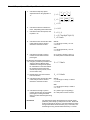
As Exhibit 2-11 shows, in addition to the factors discussed in the previous section
relating to vehicle capacity, there are other factors which must be considered when
calculating person capacity.
Exhibit 2-11
Person Capacity Factors
Operator
Policy
Number
of
Passenger
Demand
Characteristics
Loading Areas
Person
Capacity
Number
Vehicleof
Capacity
Loading
Areas
Part 2/BUS TRANSIT CAPACITY
Page 2-13
Chapter 1—Bus Capacity Basics
7UDQVLW&DSDFLW\DQG4XDOLW\RI6HUYLFH0DQXDO
Operator Policy
Increasing the maximum
allowed passenger load
increases person capacity,
but decreases quality of
service.
Two factors directly under the control of the bus operator are the maximum
passenger load allowed on buses and the service frequency. An operator whose policy
requires all passengers to be seated will have a lower potential passenger capacity for a
given number of buses, than one whose policy allows standees. (The quality of service
experienced by passengers, though, will be higher with the first operator.) The bus
frequency determines how many passengers can actually be carried, even though a bus
stop or lane may be physically capable of serving more buses than are actually scheduled.
Passenger Demand Characteristics
How passenger demand is distributed spatially along a route and how it is distributed
over time during the analysis period affects the number of boarding passengers that can be
carried. The spatial aspect of passenger demand, in particular, is why passenger capacity
must be stated for a given location, not for a route or a street as a whole.
During the period of an hour, passenger demand will fluctuate. The peak hour factor
reflects passenger demand volumes over (typically) a 15-minute period during the hour. A
bus system should be designed to provide sufficient capacity to accommodate this peak
passenger demand. However, since this peak demand is not sustained over the entire hour
and since not every bus will experience the same peak loadings, actual person capacity
during the hour will be less than that calculated using peak-within-the-peak demand
volumes.
The average passenger trip length affects how many passengers may board a bus as it
travels its route. If trip lengths tend to be long (passengers board near the start of the route
and alight near the end of the route), buses on that route will not board as many
passengers as a route where passengers board and alight at many locations. However, the
total number of passengers on board buses on each route at their respective maximum
load points may be quite similar.
The distribution of boarding passengers among bus stops affects the dwell time at
each stop. If passenger boardings are concentrated at one stop, the vehicle capacity of a
bus lane will be lower, since that stop’s dwell time will control the vehicle capacity (and,
in turn, the person capacity) of the entire lane. Vehicle capacity (and person capacity at
the maximum load point) is greater when passenger boarding volumes (and, thus, dwell
times) are evenly distributed among stops.
Vehicle Capacity
The vehicle capacity of various facilities used by buses—loading areas, bus stops,
and bus lanes—set an upper limit to the number of passengers that may use a bus stop or
may be carried past a bus route’s or bus lane’s maximum load point.
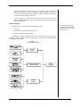
The relationship between the vehicle capacity of bus facilities and the elements of
person capacity described above is illustrated in Exhibit 2-12:
Exhibit 2-12
Person Capacity Calculation Process
Bus stop and bus lane
person capacities are
constrained by the maximum
vehicle capacities of those
locations. Bus route person
capacity is usually
constrained by the service
frequency set by the transit
operator.
Part 2/BUS TRANSIT CAPACITY
Page 2-14
Chapter 1—Bus Capacity Basics
7UDQVLW&DSDFLW\DQG4XDOLW\RI6HUYLFH0DQXDO
FUNDAMENTAL CAPACITY CALCULATIONS
Regardless of the kind of bus facility being analyzed, there are some fundamental
capacity calculations common to each. This section presents these calculation procedures,
which will be used throughout Chapters 3-5.
Vehicle Capacity
Dwell Time
Three methods can be used to determine bus dwell times:
1.
2.
3.
Field measurements. This method is best suited for determining the capacity of
an existing bus route.
Default values. This method is best suited for future planning when reliable
estimates of future passenger boarding and alighting volumes are not available.
Calculation. This method is suitable for estimating dwell times when passenger
boarding and alighting counts or estimates are available.
Method 1: Field Measurements
The most accurate way to determine bus dwell times at a stop is to measure them
directly. An average (mean) dwell time and its standard deviation can be determined from
a series of observations. Appendix A presents a methodology for measuring bus dwell
times in the field.
Best for evaluating existing bus
routes. See Appendix A for
details.
Method 2: Default Values
If field data or passenger counts are unavailable for a bus stop, the following
representative values can be used to estimate dwell time: 60 seconds per CBD, transit
center, major on-line transfer point, or major park-and-ride stop, 30 seconds per major
outlying stop, and 15 seconds per typical outlying stop.(R20)
Best for future planning when
reliable passenger estimates are
unavailable.
Suitable when passenger counts
or estimates are available.
Method 3: Calculation
This method requires that passenger counts or estimates be available, categorized by
the number of boarding and alighting passengers.
Step 1: Obtain hourly passenger volume estimates. These estimates are required only
for the highest-volume stops. When skip-stop operations are used, estimates are needed
for the highest-volume stops in each skip-stop sequence.
Step 2: Adjust hourly passenger volumes for peak passenger volumes. Equation 2-1
shows the peak hour factor (PHF) calculation method. Typical peak-hour factors range
from 0.60 to 0.95 for transit lines.(R9,R13) A PHF close to 1.0 may well indicate system
overload (underservicing) and reveal the potential for more service. If buses operate at
less than 15-minute headways, the denominator of Equation 2-1 should be adjusted
appropriately (e.g., 3P20 for 20-minute headways). Equation 2-2 adjusts hourly passenger
volumes to reflect peak-within-the-peak conditions.
PHF =
P
4 P15
Equation 2-1
P15 =
P
4( PHF )
Equation 2-2
Part 2/BUS TRANSIT CAPACITY
Page 2-15
Chapter 1—Bus Capacity Basics
7UDQVLW&DSDFLW\DQG4XDOLW\RI6HUYLFH0DQXDO
where:
PHF
P
P15
=
=
=
peak hour factor;
passenger volume during the peak hour (p); and
passenger volume during the peak 15 minutes (p).
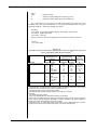
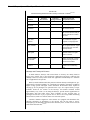
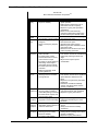
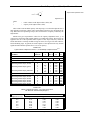
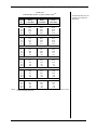
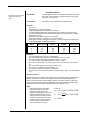
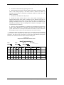
Step 3: Determine the base passenger boarding and alighting time. This time can be
estimated using values given in Exhibit 2-13 or by using the following values for typical
operating conditions—single-door loading, pay on bus:
Boarding
2.0 seconds pre-payment (includes bus pass, free transfer, pay-on-leave)
2.6 seconds single ticket/token
3.0 seconds exact fare
Add 0.5 seconds to the above boarding times if standees are present on the bus.
Alighting
1.7 to 2.0 seconds
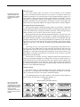
Exhibit 2-13
Typical Bus Passenger Boarding and Alighting Service Times for Selected Bus Types and
(R4)
Door Configurations (Seconds per Passenger)
Available Doors or
Channels
Bus Type
Conventional (rigid body)
Articulated
Number
1
1
2
2
2
4
3
2
2
6
Special Single Unit
6
Location
Front
Rear
Front
Rear
Front, Rear d
Front, Rear f
Front, Rear,
Center
Rear
Front, Center d
Front, Rear,
Center e
3 Double
Doors h
Typical Boarding
Typical
Service Times a (s)
Alighting
Single Service Times
(s)
Prepayment b Coin Fare
2.0
2.6 to 3.0
1.7 to 2.0
2.0
NA
1.7 to 2.0
1.2
1.8 to 2.0
1.0 to 1.2
1.2
NA
1.0 to 1.2
1.2
NA
0.9
0.7
NA
0.6
0.9f
NA
0.8
1.2g
----0.5
NA
----NA
----0.6
0.4
0.5
NA
0.4
NA: data not available
a
Typical interval in seconds between successive boarding and alighting passengers. Does not allow
for clearance times between successive buses or dead time at stop.
b
Also applies to pay-on-leave or free transfer situation.
c
Not applicable with rear-door boarding. Higher end of range is for exact fare.
d
One each.
e
Two double doors each position.
f
Less use of separated doors for simultaneous loading and unloading.
g
Double door rear loading with single exits; typical European design. Provides one-way flow within
vehicle, reducing internal congestion. Desirable for line-haul, especially if two-person operation is
feasible. May not be best configuration for busway operation.
h
Examples: Denver 16th Street Mall shuttle, airport buses used to shuttle passengers to planes.
Typically low-floor buses with few seats serving short, high-volume passenger trips.
Part 2/BUS TRANSIT CAPACITY
Page 2-16
Chapter 1—Bus Capacity Basics
7UDQVLW&DSDFLW\DQG4XDOLW\RI6HUYLFH0DQXDO
Step 4: Adjust the passenger boarding and alighting times for special conditions.
Multiply the base boarding and/or alighting times, as appropriate, by the following factors
if the corresponding condition occurs:
•
Heavy two-way flow through a single door: 1.2 (R9)
•
Double-stream door: 0.6 (R17,R18)
•
Low-floor bus: 0.85 (R15)
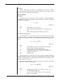
Step 5: Calculate the dwell time. The dwell time is the time required to serve
passengers at the busiest door, plus the time required to open and close the doors. A value
of 2 to 5 seconds for door opening and closing is reasonable for normal operations.(R4,R19)
The number of boarding and alighting passengers per bus through the busiest door during
the peak-within-the-peak (typically 15 minutes), Pb and Pa, are determined by the
proportions of boarding and alighting passengers per bus during the peak period.
t d = Pa t a + Pb t b + t oc
Equation 2-3
where:
td
Pa
=
=
ta
Pb
=
=
tb
toc
=
=
dwell time (s);
alighting passengers per bus through the busiest door
during the peak 15 minutes (p);
passenger alighting time (s/p);
boarding passengers per bus through the busiest door
during the peak 15 minutes (p);
passenger boarding time (s/p); and
door opening and closing time (s).
Impact of Wheelchair Accessibility on Dwell Time
All new transit buses in the U.S. are equipped with wheelchair lifts or ramps. When a
lift is in use, the door is blocked from use by other passengers. Typical wheelchair lift
cycle times are 60 to 200 seconds, while the ramps used in low-floor buses reduce the
cycle times to 30 to 60 seconds (including the time required to secure the wheelchair
inside the bus). The higher cycle times relate to a small minority of inexperienced or
severely disadvantaged users. When wheelchair users regularly use a bus stop to board or
alight, the wheelchair lift time should be added to the dwell time.
Impact of Bicycles on Dwell Time
Some transit systems provide folding bicycle racks on buses. When no bicycles are
loaded, the racks typically fold upright against the front of the bus. (Some systems also
use rear-mounted racks, and a very few allow bikes on-board on certain long-distance
routes.) When bicycles are loaded, passengers deploy the bicycle rack and load their
bicycles into one of the available loading positions (typically two are provided). The
process takes approximately 20 to 30 seconds. When bicycle rack usage at a stop is
frequent enough to warrant special treatment, a bus’ dwell time is determined using the
greater of the passenger boarding/alighting time or the bicycle loading/unloading time.
Clearance Time
Clearance time includes two components, (1) the time for a bus to start up and travel
its own length while exiting a bus stop, and for off-line stops, (2) the re-entry delay
associated with waiting for a sufficient gap in traffic to allow a bus to pull back into the
travel lane. Various studies have evaluated these factors, either singly or as a whole.
Scheel and Foote found that bus start-up times range from 2 to 5 seconds.(R30) The time
for a bus to travel its own length after stopping is approximately 5 to 10 seconds,
Part 2/BUS TRANSIT CAPACITY
Page 2-17
Door opening and closing time is
incorporated into the dwell time,
rather than the clearance time.
Chapter 1—Bus Capacity Basics
7UDQVLW&DSDFLW\DQG4XDOLW\RI6HUYLFH0DQXDO
depending on acceleration and traffic conditions. TCRP Report 26 recommends a range
of 10-15 seconds for clearance time.(R29)
Clearance time is the sum of
start-up and exiting time and
re-entry delay.
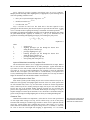
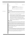
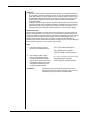
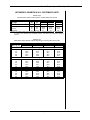
Start-up and exiting time may be assumed to be 10 seconds. Re-entry delay can be
measured in the field or, at locations where buses re-enter a traffic stream, may be
estimated from Exhibit 2-14, based on traffic volumes in the adjacent travel lane. If buses
must wait for a queue from a signal to clear before they can re-enter the street, Exhibit 214 should not be used; instead, re-entry delay should be estimated using the average
queue length (in vehicles), the saturation flow rate, and the start-up lost time.
Exhibit 2-14
Average Bus Re-Entry Delay into Adjacent Traffic Stream (Random Vehicle Arrivals)
Adjacent Lane
Mixed Traffic Volume (veh)
100
200
300
400
500
600
700
800
900
1,000
Exhibit 2-14 applies only to
off-line stops where buses
must yield to other traffic
when re-entering a street,
and only when the stop is
located away from the
influence of a queue from a
signalized intersection.
SOURCE:
Re-entry delay can be
reduced or eliminated by
using on-line stops, queue
jumps at signals, or laws
requiring traffic to yield to
buses.
Average Re-Entry Delay
(s)
0
1
2
3
4
5
7
9
11
14
Computed using 1997 HCM unsignalized intersection methodology (minor street right
turn at a stop sign), assuming a critical gap of 7 seconds and random vehicle arrivals.
Delay based on 12 buses stopping per hour.
Some states in the U.S. have passed laws requiring other traffic to yield to transit
vehicles that are signaling to exit a stop. In these locations, the re-entry delay can be
reduced or even eliminated, depending on how well motorists comply with the law.
Transit priority measures, such as queue jumps at signals (see Chapter 2), can also reduce
or eliminate re-entry delay.
Coefficient of Variation of Dwell Times
The coefficient of variation of
dwell times is the standard
deviation of dwell times
divided by the mean dwell
time.
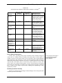
Based on field observations of bus dwell times in several U.S. cities reported in
TCRP Report 26,(R29) the coefficient of variation of dwell times (the standard deviation of
dwell times divided by the mean dwell time) typically ranges from 40% to 80%, with 60%
recommended as an appropriate value in the absence of field data.
Failure Rate
One-tail normal variate, Za.
The probability that a queue of buses will not form behind a bus stop, or failure rate,
can be derived from basic statistics. The value Za represents the area under one “tail” of
the normal curve beyond the acceptable levels of probability of a queue forming at a bus
stop. Typical values of Za for various failure rates are shown in Exhibit 2-15. A design
failure rate should be chosen for use in calculating a loading area’s capacity. Higher
design failure rates increase bus stop capacity at the expense of schedule reliability.
Capacity occurs under normal conditions at a 25% failure rate.(R9,R23)
Part 2/BUS TRANSIT CAPACITY
Page 2-18
Chapter 1—Bus Capacity Basics
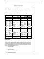
7UDQVLW&DSDFLW\DQG4XDOLW\RI6HUYLFH0DQXDO
Exhibit 2-15
(R29)
Values of Percent Failure Associated With Za
Failure Rate
1.0%
2.5%
5.0%
7.5%
10.0%
15.0%
20.0%
25.0%
30.0%
50.0%
Za
2.330
1.960
1.645
1.440
1.280
1.040
0.840
0.675
0.525
0.000
Suggested values of Za are the following:(R29)
Suggested design failure rates.
•
CBD stops. Za values of 1.440 down to 1.040 should be used. They result in
probabilities of 7.5 to 15 percent, respectively, that queues will develop.
•
Outlying stops. A Za value of 1.960 should be provided wherever possible,
especially when buses must pull into stops from the travel lane. This results in
queues beyond bus stops only 2.5 percent of the time. Za values down to 1.440
are acceptable, however.
Loading Areas
The maximum number of buses per loading area per hour is:(R29)
Bbb =
Loading area vehicle capacity.
3,600( g / C )
t c + ( g / C)t d + Z a c v t d
Equation 2-4
where:
Bbb
g/C
=
=
tc
td
Za
=
=
=
cv
=
maximum number of buses per loading area per hour;
ratio of effective green time to total traffic signal cycle
length (1.0 for a stop not at a signalized intersection);
clearance time between successive buses (s);
average (mean) dwell time (s);
one-tail normal variate corresponding to the probability
that queues will not form behind the bus stop; and
coefficient of variation of dwell times.
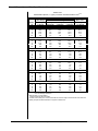
Exhibit 2-16 presents the estimated number of buses that can use a bus loading area
for g/C ratios of 0.5 and 1.0 (the ratio of green signal time to the total traffic signal cycle
length). Values are tabulated for dwell times ranging from 15 to 120 seconds. Values for
g/C times between 0.5 and 1.0 can be interpolated; values for g/C times less than 0.5 and
for other dwell times can be computed directly from Equation 2-4. These maximum
capacities assume adequate loading area and bus stop geometry. Guidelines for the
spacing, location, and geometric design of bus stops are given in TCRP Report 19.(R6)
These guidelines must be carefully applied to assure both good traffic and transit
operations.
Part 2/BUS TRANSIT CAPACITY
Page 2-19
Chapter 1—Bus Capacity Basics
7UDQVLW&DSDFLW\DQG4XDOLW\RI6HUYLFH0DQXDO
Exhibit 2-16
Estimated Maximum Capacity of Loading Areas (Buses/h)
Dwell Time (s)
15
30
45
60
75
90
105
120
NOTE:
g/C = 0.5
63
43
32
26
22
19
16
15
g/C = 1.0
100
63
46
36
30
25
22
20
Assumes 15-second clearance time, 25% queue probability, and 60% coefficient of
variation of dwell times.
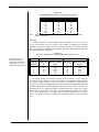
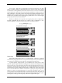
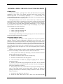
Bus Stops
As shown in Exhibit 2-17, increasing the number of loading areas at a linear bus stop
has an ever-decreasing effect on capacity as the number of loading areas increases
(doubling the number of loading areas at a linear bus stop does not double capacity).
When more than three loading areas are required, sawtooth, pull-through, or other nonlinear designs should be considered.
Exhibit 2-17
(R19,R21,R23)
Efficiency of Multiple Linear Loading Areas at Bus Stops
Sawtooth and other nonlinear designs are more
effective than linear loading
areas when four or five
loading areas are required.
Loading
Area #
1
2
3
4
5
On-Line Loading Areas
# of Cumulative
Efficiency Effective Loading
%
Areas
100
1.00
85
1.85
60
2.45
20
2.65
5
2.70
Off-Line Loading Areas
# of Cumulative
Efficiency
Effective Loading
%
Areas
100
1.00
85
1.85
75
2.60
65
3.25
50
3.75
NOTE: On-line values assume that buses do not overtake each other.
The off-line loading area efficiency factors given in Exhibit 2-17 are based on
experience at the Port Authority of New York and New Jersey’s Midtown Bus Terminal.
The on-line loading efficiency factors are based on simulation(R23) and European
experience.(R16) The exhibit suggests that four or five on-line linear loading areas have the
equivalent effectiveness of three loading areas. Note that to provide two “effective” online loading areas, three physical loading areas would need to be provided, since partial
loading areas are never built. Once again, it should be noted that Exhibit 2-17 applies
only to linear loading areas. All other types of multiple loading areas are 100%
efficient—the number of effective loading areas equals the number of physical loading
areas.
Part 2/BUS TRANSIT CAPACITY
Page 2-20
Chapter 1—Bus Capacity Basics
7UDQVLW&DSDFLW\DQG4XDOLW\RI6HUYLFH0DQXDO
The vehicle capacity of a bus stop in buses per hour is given by Equation 2-5:
Bs = N eb Bbb = N eb
3,600( g / C )
t c + ( g / C)t d + Z a cv t d
Equation 2-5
where:
Bs
Neb
=
=
maximum number of buses per bus stop per hour; and
number of effective loading areas, from Exhibit 2-17.
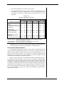
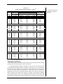
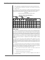
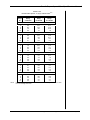
Exhibit 2-18 provides estimated capacities of on-line bus stops. This exhibit shows
the number of buses per hour for various numbers of loading areas, dwell times, and g/C
ratios. The maximum capacities attainable are 3.0 times those of a single loading area.
Exhibit 2-18
Estimated Maximum Capacity of On-Line Linear Bus (bus/h)
Dwell
Time
(s)
30
60
90
120
NOTE:
1
g/C
0.50
43
26
19
15
g/C
1.00
63
36
25
20
Number of On-Line Linear Loading Areas
2
3
4
g/C
g/C
g /C
g/C
g/C
g/C
0.50
1.00
0.50
1.00
0.50
1.00
79
117
105
154
113
167
48
67
64
89
69
96
35
47
46
62
49
67
27
36
36
48
39
52
5
g/C
0.50
115
70
50
39
g/C
1.00
170
98
69
53
Assumes 15-second clearance time, 25% queue probability, and 60% coefficient of
variation of dwell times. To obtain the vehicle capacity of non-linear on-line bus stops,
multiply the one-loading-area values by the number of loading areas provided.
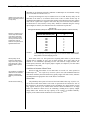
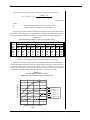
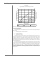
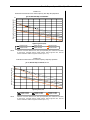
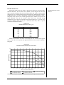
Exhibit 2-19 provides a further guide for estimating on-line linear bus stop capacity.
It shows the number of buses per hour for selected dwell times and g/C ratios based on a
15-second clearance time. Increasing the number of linear loading areas has a much
smaller effect on changes in capacity than reducing dwell times. Note that for dwell times
greater than 60 seconds, the differences between a g/C of 0.5 and 1.0 are small.
Exhibit 2-19
Bus Stop Maximum Vehicle Capacity
Related to Dwell Times and Number of Loading Areas
180
Vehicle Capacity (bus/h)
160
140
120
30-s dwell, g/C = 1.0
30-s dwell, g/C = 0.5
100
60-s dwell, g/C = 1.0
80
60-s dwell, g/C = 0.5
120-s dwell, g/C = 1.0
60
120-s dwell, g/C = 0.5
40
20
0
1
2
3
4
5
Number of Linear On-Line Loading
Areas
Part 2/BUS TRANSIT CAPACITY
Page 2-21
Chapter 1—Bus Capacity Basics
7UDQVLW&DSDFLW\DQG4XDOLW\RI6HUYLFH0DQXDO
Bus Lanes
Bus lane vehicle capacity procedures vary, depending on the facility type. Chapters
3-5 present bus lane capacity procedures for busways and freeway HOV lanes, exclusive
arterial street bus lanes, and mixed traffic situations.
Person Capacity
Bus Stops
The person capacity of a bus stop is related to the number of people boarding and
alighting at the bus stop, which influences the vehicle capacity of the bus stop. Equation
2-6 shows this relationship:
Ps = B s P15
Equation 2-6
where:
Ps
Bs
=
=
P15
=
person capacity of a bus stop (p/h);
vehicle capacity of the bus stop (buses/h), from Equation 2-5;
and
peak 15-minute passenger interchange per bus (p/bus).
Bus Routes and Bus Lanes
The person capacity of a bus route or bus lane at its maximum load point under
prevailing conditions is determined by the allowed passenger loading set by operator
policy and by the number of buses operated during the analysis period (typically one
hour):
Pmlp = Pmax f mlp (PHF )
Equation 2-7
where:
Pmlp
=
Pmax
fmlp
=
=
PHF
=
person capacity of a bus route or bus lane at its maximum
load point under prevailing conditions (p/h);
maximum allowed passenger loading per bus (p/bus);
bus frequency on the route or the bus lane at its maximum
load point (buses/h); and
peak hour factor.
The person capacity of a bus route or bus lane, in terms of number of boarding
passengers during the analysis period, may be considerably greater than the person
capacity given by Equation 2-7, if typical passenger trip lengths are short relative to the
length of the bus route or bus lane.
The maximum person capacity of a bus lane at its maximum load point is determined
by the bus lane’s maximum vehicle capacity:
Pmlp , max = Pmax B ( PHF )
Equation 2-8
Part 2/BUS TRANSIT CAPACITY
where:
Pmlp,max
=
B
=
maximum person capacity of a bus route or bus lane at its
maximum load point (p/h); and
bus lane vehicle capacity (bus/h), from the appropriate
Chapter 3, 4, 5 procedure.
Page 2-22
Chapter 1—Bus Capacity Basics
7UDQVLW&DSDFLW\DQG4XDOLW\RI6HUYLFH0DQXDO
PLANNING APPLICATIONS
Exhibit 2-20 summarizes the bus vehicle and person capacity factors and calculations
identified in this chapter and suggests ways that each can be improved to provide
additional capacity. Note that in some cases, increasing capacity requires a trade-off with
decreased quality of service.
Exhibit 2-20
Factors Influencing Bus Capacity
Item
Dwell Time
Clearance Time
Coefficient of Variation
Failure Rate
Loading Area Capacity
Bus Stop Capacity
Bus Lane Capacity
Bus Speeds
Ways To Improve Each Item
CAPACITY FACTORS
• Greater use of pre-paid fares
• Use low-floor vehicles
• Encourage one-way door flows on two-door buses
• Provide multiple-stream doors for boarding and
alighting
• Increase bus frequency to reduce the number of
standees
• Implement proof-of-payment fare collection
• Use on-line stops*
• Enact and enforce laws that require cars to yield to
buses re-entering a street
• Implement queue jumps at traffic signals
• Generally constant for a given area
• Increase the number of loading areas at a stop
• Schedule fewer buses per hour using the stop**
CALCULATED RESULTS
• Reduce dwell time
• Implement transit priority treatments
• Increase the accepted failure rate*
• Increase loading area capacity
• Use off-line loading areas*
• Use sawtooth or pull-through loading areas
• Increase the number of loading areas
• Increase the capacity of the critical stop
• Reserve lanes for buses
• Platoon buses
• Implement skip-stop operation
• Prohibit right turns by automobiles
• Reduce dwell time
• Implement transit preferential treatments
• Balance the number of stops with passenger
convenience and demand
• Implement skip-stop operation
*Measures that may negatively affect other items in the list if implemented.
**Measure that improves the failure rate, but decreases capacity.
The observed peak-hour bus movements along freeways and city streets, and to or
from bus terminals provide guidelines for estimating the capacity of similar facilities.
They also provide means of checking or verifying more detailed capacity calculations.
General guidelines for planning purposes follow:
Suggested arterial street bus service volume varies based on actual operating
experience. Suggested service volumes are given in Exhibit 2-21. This table gives
representative service volumes for downtown streets and arterial streets leading to the city
center for each level of service. Where stops are not heavily patronized, as along outlying
arterial streets, volumes could be increased by about 25 percent.
Part 2/BUS TRANSIT CAPACITY
Page 2-23
Roadway bus capacity.
Chapter 1—Bus Capacity Basics
7UDQVLW&DSDFLW\DQG4XDOLW\RI6HUYLFH0DQXDO
Exhibit 2-21
Suggested Bus Flow Service Volumes for Planning Purposes
(R12,R14)
(Flow Rates For Exclusive or Near-Exclusive Lane)
These service volumes may be
used for planning purposes. More
precise values for operations and
design purposes should be
computed from the capacity
relationships and procedures
presented later in Part 2.
Service Volume
bus/lane/h
ARTERIAL STREETS
Free Flow
25 or less
Stable Flow, Unconstrained
26 to 45
Stable Flow, Interference
46 to 75
Stable Flow, Some Platooning
76 to 105
Unstable Flow, Queuing
106 to 135
Forced Flow, Poor Operation
over 135*
CBD STREETS
Free Flow
20 or less
Stable Flow, Unconstrained
21 to 40
Stable Flow, Interference
41 to 60
Stable Flow, Some Platooning
61 to 80
Unstable Flow, Queuing
81 to 100
Forced Flow, Poor Operation
over 100*
Description
The values for forced flow
conditions should not be used for
planning or design. They are
merely given for comparative
purposes.
Average
bus/lane/h
15
35
60
90
120
150*
15
30
50
70
90
110*
*Results in more than one-lane operation.
Person capacity.
The people per hour that can be served by varying bus flow rates and passenger load
factors are given in Exhibit 2-22. This table provides a broad person-capacity planning
guide assuming that key boarding points are sufficiently dispersed to achieve these bus
loads. It suggests maximum person-flow rates of about 6,450 people per hour per lane on
downtown streets and 8,700 people per hour per lane on arterial streets. Corresponding
maximum values for seated passenger flow rates are 4,300 and 5,800 people respectively.
Exclusive use of articulated buses would increase these values by 15 to 20 percent.
Exhibit 2-22
Maximum Bus Passenger Service Volumes For Planning Purposes
(Hourly Flow Rates Based on 43 Seats Per Bus)
Buses per
Hour
25 or less
26 to 45
46 to 75
76 to 105
106 to 135
20 or less
21 to 40
41 to 60
61 to 80
81 to 100
Peak-hour factor.
Passengers/Seat
0.000.510.761.010.50
0.75
1.00
1.25
ARTERIAL STREETS
535
805
1,075
1,340
965
1,450
1,935
2,415
1,610
2,415
3,225
4,030
2,255
3,385
4,515
5,640
2,900
4,350
5,805
7,255
CBD STREETS
430
645
860
1,075
860
1,290
1,720
2,150
1,290
1,935
2,580
3,225
1,720
2,580
3,440
4,300
2,150
3,225
4,300
5,375
1.261.50
1,610
2,900
4,835
6,770
8,705
1,290
2,580
3,870
5,160
6,450
These person-flow rates indicate the number of people that can be carried, assuming
uniform flow during the peak hour. Appropriate peak hour factors should be used to
discount these values to reflect flow variations within the 15-minute peak period.
Part 2/BUS TRANSIT CAPACITY
Page 2-24
Chapter 1—Bus Capacity Basics
7UDQVLW&DSDFLW\DQG4XDOLW\RI6HUYLFH0DQXDO
2. OPERATING ISSUES
INTRODUCTION
This chapter presents operating issues that influence the results of the capacity
procedures presented in the remainder of Part 2. Factors under the direct control of bus
operators are the allowed passenger loads on a bus and whether or not a skip-stop pattern
is used on streets with high bus volumes. Bus preferential treatments at intersections and
on roadway segments, in order to be implemented, require the cooperation of bus
operators and the agencies responsible for streets and roads.
BUS OPERATIONS
Passenger Loads
From a capacity perspective, the allowed passenger load on a bus (set by policy)
constrains the number of people that a given number of buses can carry. From a
passenger’s perspective, loading reflects the comfort level of the on-board portion of a
bus trip—both in terms of being able to find a seat and in overall crowding levels within
the bus. From a transit operator’s perspective, liability concerns and the desire to provide
every customer with a seat for high-speed or long-distance services may cause the
operator to set the allowed loading at levels lower than what riders might tolerate.
The impacts of all three of these perspectives on transit capacity are addressed in this
section. The quality of service impacts of passenger loading are addressed in Part 5 of this
manual.
Guidelines
The passenger load is simply the number of passengers on a single transit vehicle.
Much work uses the occupancy of the vehicle relative to the number of seats, expressed as
a load factor. A factor of 1.0 means that all of the seats are occupied. The importance of
vehicle loading varies by the type of service. In general, bus transit provides load factors
below 1.0 for long-distance commute trips and high-speed, mixed-traffic operations.
Inner-city service can approach a load factor of 2.0 (but more typically 1.5), while other
services are in between. Typical bus vehicle types, dimensions, and passenger capacities
are given in Exhibit 2-23.
Load factor.
Exhibit 2-23
Characteristics of Bus Transit Vehicles—United States and Canada
Bus Type
Length Width
(m)
(m)
Typical Capacity
Seats
Standees
Total
An alternative table using U.S.
customary units appears in
Appendix B.
Small Bus/Minibus
Transit Bus
5.6-9.1 2.0-2.4
8-30
0-10
8-40
10.7
2.4-2.6
30-35
20-30
50-60
12.2
2.6
35-50
30-40
65-75
(low floor)
12.2
2.4
30-40
25-40
55-70
(articulated)
18.3
2.4-2.6
65
55
120
NOTE: In any transit vehicle, the total passenger capacity can be increased by removing seats
and by making more standing room available; however, this lowers the passengers’ quality
of service. The upper ends of the total capacity ranges represent crush capacity and
should not be used for transit capacity calculations.
A typical 12-meter (40-foot) urban transit bus can normally seat 43 passengers and
can carry up to 37 additional standees if all of the aisle circulation space is filled.
Similarly, an 18-meter (60-foot) articulated bus can carry 65 seated passengers and 55
standees. However, bus operator policy often limits the number of standees to levels
below this theoretically offered, or crush capacity.
Part 2/BUS TRANSIT CAPACITY
Page 2-25
Chapter 2—Operating Issues
7UDQVLW&DSDFLW\DQG4XDOLW\RI6HUYLFH0DQXDO
Maximum schedule loads.
Maximum schedule load is synonymous with “capacity,” assuming a reasonable
number of standees. It represents the upper limit for scheduling purposes. Maximum
scheduled loads are typically 125 to 150 percent of a bus’ seating capacity (e.g., 54-64
passengers on a typical 12-meter or 40-foot bus).
Crush loads.
Crush loads, typically loads above 150 percent of a bus’ seating capacity, subject
standees and other passengers to unreasonable discomfort. Such loads are unacceptable to
passengers. Crush loads prevent circulation of passengers at intermediate stops and so
induce delay and reduce vehicle capacity. Although crush loading represents the
theoretically offered capacity, it cannot be sustained on every bus for any given period,
and it exceeds the maximum utilized capacity. Therefore, crush loads should not be used
for transit capacity calculations. Note, however, that when maximum schedule loads are
used, some buses will experience crush loading, due to the peaking characteristics of
passenger demand.
Minimum passenger space
requirements.
Design guidelines for seats and passenger areas in transit vehicles are based on
human factors. Part 5 addresses the quality of service aspects of passenger loading. For
buses, comfortable loading for design should provide at least 0.50 m2/passenger (5.4 ft2/p)
and maximum schedule loads should provide a minimum of 0.40 m2/p (4.3 ft2/p), where
relatively short trips allow standees.(R9) The “comfortable loading” figure provides a
reasonable balance between operating economy and passenger comfort and is consistent
with the value suggested by Pushkarev and Zupan for a realistic passenger capacity for
rapid transit lines.(R27) However, high-speed express bus service should not allow
standees; hence, their scheduling should be guided by the number of seats provided.
Skip-Stop Operation
When buses stop at every curbside bus stop in an on-line loading area arrangement,
using the adjacent lane only becomes necessary for passing obstructions in the curbside
lane. The ability to spread out stops, alternating route stop patterns along an arterial
street, can substantially improve bus speeds and capacities.
Many large transit systems have instituted two- or three-block stop patterns for bus
stops along arterial streets. This block skipping pattern allows for a faster trip through the
section and reduces the number of buses stopping at each bus stop.
Exhibit 2-24 illustrates the skip-stop pattern used by Tri-Met in Portland, Oregon on
its Fifth and Sixth Avenue Transit Mall in 1997. Each street uses a repeating pattern of
three or four bus stops. Each bus stop contains two loading areas. All routes headed for a
particular portion of the metropolitan area use a particular set of stops, which are
designated by a colored symbol (for example, a brown beaver) on bus stop signs, bus
schedules, and maps. As shown in Exhibit 2-24, other bus stop signing systems can also
be used, such as Denver’s “X-Y-Z” system.
Capacity adjustment for the
availability of the adjacent
lane.
These alternate block stopping patterns enable the bus lane capacity to nearly equal
the sum of the capacities of the stops involved. Thus an arterial with an alternate twoblock stopping pattern would, ideally, have a capacity equal to the sum of the two stops,
assuming unimpeded use of the adjacent lane. In reality, this may not always be possible
because of the irregularity of bus arrivals and traffic control delays. (To effectively
double the capacity of a segment with a 3-bus loading area capacity at each stop by
instituting a two-block A-B stop pattern, three A-pattern buses must arrive at the upstream
entry to the section during one signal cycle, followed by three B-pattern buses.) Buses
alternating stops must also be able to utilize the adjacent traffic lane to bypass stopped
buses. They may be impeded in this maneuver when the adjacent lane operates at or near
capacity.
Part 2/BUS TRANSIT CAPACITY
Page 2-26
Chapter 2—Operating Issues
7UDQVLW&DSDFLW\DQG4XDOLW\RI6HUYLFH0DQXDO
Exhibit 2-24
Example Skip-Stop Pattern and Bus Stop Signing
th
th
Portland, Oregon 5 and 6 Avenue Bus Mall
5th Avenue
n
Statio
Union trak) W IRVING
N
OYT
(Am
NW H
LISAN
NW G
ERS
LAND
NW F
To
n
Unio n
Statio
4
9
10
14
17
19
31
32
33
35
38
40
96
99X
54
55
56
57
58
59
60
88
89
91X
92X
94X
1
4
5
17
40
8
9
10
12
19
33
The Portland 5th and 6th Avenue
Bus Mall is depicted on the map
(1997 configuration). All buses
heading to a particular portion of
the Portland area use the same
stop, which is indicated by a
colored symbol on maps and bus
stops, such as the “orange deer”
pictured.
Local buses stop every two
blocks, with four sets of stops
southbound on Fifth Avenue (two
in each block) and three sets of
stops northbound on Sixth
Avenue. Express buses (routes
ending in “X”) stop every four
blocks.
TT
VERE
NW E
AVIS
NW D
OUCH
NW C
To
n
Unio
n
Statio
1
5
8
12
43
45
95X
6th Avenue
E
RNSID
W BU
The number of buses using the
“orange deer” stops decreased in
the fall of 1998, following the
opening of the Westside MAX
light rail extension, which
replaced many of the routes using
those stops.
SW ASH
SW PINE
To
Union
Station
SW OAK
To
Union
Station
SW STARK
SW WASHINGTON
To
Union
Station
SW ALDER
SW MORRISON
To
Union
Station
Other systems for designating
bus stops in a skip-stop sequence
are also possible, such as
Denver’s X-Y-Z system pictured
to the left.
SW YAMHILL
SW TAYLOR
To
Union
Station
SW SALMON
SW MAIN
SW MADISON
Part 2/BUS TRANSIT CAPACITY
Page 2-27
Chapter 2—Operating Issues
7UDQVLW&DSDFLW\DQG4XDOLW\RI6HUYLFH0DQXDO
ROADWAY OPERATIONS
Much attention has been paid to expediting transit flow by providing various forms of
priority treatment. Such treatments are aimed at improving schedule adherence and
reducing travel times and delays for transit users. They may attract new riders, increase
transit capacity, and/or improve the transit quality of service.
Successful priority measures are usually characterized by:
•
•
•
•
•
•
•
•
an intensively developed downtown area with limited street capacity and high
all-day parking costs,
a long-term reliance on public transport,
highway capacity limitations on the approaches to downtown,
major water barriers that limit road access to the CBD and channel bus flows,
fast non-stop bus runs for considerable distances,
bus priorities on approaches to or across water barriers,
special bus distribution within the CBD (often off-street terminals), and
active traffic management, maintenance, operations, and enforcement
programs.(R21)
Bus Preferential Treatments at Intersections
When buses operate in mixed traffic, as is typical, the interference caused by general
traffic decreases bus speeds and lowers overall bus vehicle and person capacity. The bus
preferential treatments described in this section compensate for these interferences by
removing or reducing sources of delay, resulting in increased bus speeds. When
considering implementing bus preferential treatments, the total change in person-delay
(including both passengers in buses and motorists) should be taken into account.
Signal Priority
Bus signal priority measures include passive systems, pre-timed modifications to the
signal system adjusted manually to determine the best transit benefit while minimizing the
impact to other vehicles, and active systems, which adjust the signal timing after sensing
the arrival of a bus. Exhibit 2-25 lists common bus signal priority systems.
Exhibit 2-25
(R1)
Bus Signal Priority Systems
Treatment
Adjust cycle length
Split phases
Areawide timing plans
Bypass metered signals
Phase extension
Early start
Special phase
Phase suppression
Preemption (Unconditional)
Preemption (Conditional)
Description
Passive Priority
Reduce cycle lengths at isolated intersections.
Apply multiple phases while maintaining original
cycle length.
Preferential progression for buses through signal
offsets.
Buses use special reserved lanes, special signal
phases, or are rerouted to non-metered signals.
Active Priority*
Increase phase time.
Reduce other phase times.
Addition of a bus phase.
Skipped non-priority phases.
Bus phase begins when all other intervals are
satisfied.
Same as above except certain conditions are used
to determine when the bus phase should begin.
*Occurs after bus detection.
Part 2/BUS TRANSIT CAPACITY
Page 2-28
Chapter 2—Operating Issues
7UDQVLW&DSDFLW\DQG4XDOLW\RI6HUYLFH0DQXDO
Active priority should only be implemented at intersections operating at less than
capacity, so that the changes to signal timing that occur each time a bus passes through
the intersection do not significantly worsen the intersection’s level of service. Automated
systems that do not require bus driver intervention are preferable, as bus drivers may not
always remember to activate the system at the intersections equipped with signal priority
equipment. When coupled with two-way data communication and automatic vehicle
location (AVL) equipment, on-bus signal priority systems can be set to activate signal
priority only when a bus is behind schedule.(R3)
Exhibit 2-26 illustrates one way that active signal priority can be implemented.
Streetside equipment can detect the bus (for example, using a transponder) or busmounted equipment can transmit a request for priority to the signal controller.
Exhibit 2-26
(R3)
Bus Signal Priority Concept
Bus approaches red signal
SIGNAL CONTROLLER
Signal controller detects bus;
terminates side street
green phase early
Bus proceeds on green signal
Queue Jump
Queue jump treatments allow buses to avoid long queues of vehicles at signalized
intersections by using right-turn lanes or long off-line bus stops to move past much of the
queue. Buses are exempted from any right-turn requirements at the intersection.
A special right-lane signal provides a green indication for a brief period of time
before the adjacent regular traffic lanes. During this time, the bus exits the right lane and
merges into the lane to the left ahead of the other traffic that had stopped for the signal.
Alternatively, the bus pulls into the right lane on a red signal and proceeds to a far-side
off-line bus stop on green, resulting in reduced delay waiting for the queue in the regular
lanes to clear the intersection. Exhibit 2-27 illustrates a typical queue jump design, while
Exhibit 2-28 shows an actual application of a queue jump. In Exhibit 2-28, the bus
receives priority from a bus lane that ends at a near-side bus stop at the intersection. In
this application, a special transit signal (the vertical bar indication adjacent to the regular
traffic signal) is used to give the bus priority, rather than a regular traffic signal.
Part 2/BUS TRANSIT CAPACITY
Page 2-29
Chapter 2—Operating Issues
7UDQVLW&DSDFLW\DQG4XDOLW\RI6HUYLFH0DQXDO
Exhibit 2-27
Bus Queue Jump Concept
Passengers board during red
BUS STOP
ONLY
EXCEPT
BUS
Bus receives green before other vehicles
BUS STOP
ONLY
EXCEPT
BUS
Other vehicles proceed a few seconds later
BUS STOP
ONLY
EXCEPT
BUS
Exhibit 2-28
Bus Queue Jump Example (Copenhagen, Denmark)
Part 2/BUS TRANSIT CAPACITY
Page 2-30
Chapter 2—Operating Issues
7UDQVLW&DSDFLW\DQG4XDOLW\RI6HUYLFH0DQXDO
Curb Extensions
Where streets have curbside parking and high traffic volumes, it may not be desirable
for a bus to pull to the curb to stop, because of the delays involved in waiting for a
sufficiently large gap in traffic that will allow the bus to pull back into the travel lane. In
these situations, the curb can be extended into the parking lane to allow buses to stop in
the travel lane to pick up and discharge passengers. The additional area curbside can be
used to provide an ADA-compliant clear area to load and unload wheelchair passengers,
to provide a bus shelter in a location that otherwise would not have enough space, and to
provide more room for passengers to stand while waiting for the bus. Curb extensions can
also create more on-street parking, as the area prior to the bus stop previously used by
buses to pull to the curb can now be used for additional parking. At intersections, curb
extensions also benefit all pedestrians by reducing the street width that must be crossed. If
bicycle lanes exist, they may need to be routed around the curb extension, creating
potential bicycle/pedestrian conflicts. Exhibit 2-29 and Exhibit 2-30 illustrate the use of
curb extensions.
Exhibit 2-29
(R3)
Curb Extension Concept
Before
Bus pulls to curb at bus stop: must wait for gap
in traffic to proceed.
P
BUS
STOP
After
Curb extended into parking lane, bus stops in
travel lane; more curbside parking available.
P
BUS
STOP
Exhibit 2-30
Curb Extension Example (Vienna, Austria)
Part 2/BUS TRANSIT CAPACITY
Page 2-31
Chapter 2—Operating Issues
7UDQVLW&DSDFLW\DQG4XDOLW\RI6HUYLFH0DQXDO
Boarding Islands
Where significant parking activity, stopped delivery vehicles, heavy right-turning
traffic volumes and other interferences slow traffic in the right lane of a street with
multiple lanes in the same direction, buses may be able to travel faster in the lane to the
left. Boarding islands allow bus stops to be located between travel lanes so that buses can
use a faster lane without having to merge into the right lane before every stop. Pedestrian
safety issues must be addressed when considering the use of boarding islands. Exhibit 231 and Exhibit 2-32 illustrate the concept and application of this treatment.
Exhibit 2-31
(R3)
Boarding Island Concept
Before
Traffic congestion in curb lane due to
parking and turning maneuvers.
After
Bus travels in faster lane, passengers load
and unload at boarding island.
Exhibit 2-32
Boarding Island Example (San Francisco)
Part 2/BUS TRANSIT CAPACITY
Page 2-32
Chapter 2—Operating Issues
7UDQVLW&DSDFLW\DQG4XDOLW\RI6HUYLFH0DQXDO
Other Measures
Other transit preferential treatments at intersections include the following:(R3)
•
Parking Restrictions. These are used in areas where high parking turnover
interferes with the flow of traffic on a street. Restricting parking will improve
transit and traffic flow, but the impacts to adjacent land uses from the loss of onstreet parking must also be considered. Parking restrictions are sometimes
applied during peak hours only, often in conjunction with bus lane operations.
•
Bus Stop Relocation. On streets with good traffic signal progression for
passenger vehicles, moving a bus stop from the near-side of an intersection to the
far-side (or vice versa) may allow buses to use the signal timing to their
advantage, passing through intersections on a green signal and dwelling on a red
signal.
•
Turn Restriction Exemptions. The most direct route for a bus may not be
possible because of left-turn restrictions at intersections, particularly where there
is insufficient room to develop left-turn lanes. If the restriction is due to traffic
congestion, rather than safety, it may be feasible to exempt buses from the
restriction without unduly impacting intersection operations.
Bus Preferential Treatments on Roadway Segments
Arterial Bus Lanes
Where there is a relatively high volume of buses operating on a roadway, coupled
with a high degree of bus and automobile congestion, exclusive bus lanes may be
considered to provide more attractive and reliable bus service. Most bus lanes take the
form of reserved bus lanes on city streets, usually in the same direction as the general
traffic flow. There are a number of bus-only streets, such as Denver’s 16th Street,
Portland’s Fifth and Sixth Avenue Transit Mall, and Vancouver’s Granville Mall.
Contraflow center lanes in Montréal, with center median waiting, are unusual but have
been successful.
Policy and cost considerations generally set the lower limit for bus volumes that
warrant priority treatments on arterials, while bus vehicle capacity sets the upper limit. A
study of bus operations in Manhattan recommended the following desirable maximum
a.m. peak hour bus volumes for arterial street bus lanes:(R22)
•
Two lanes exclusively for buses: 180 buses/hour
•
One lane exclusively for buses, partial use of adjacent lane: 100 buses/hour
•
One lane exclusively for buses, no use of adjacent lane: 70 buses/hour
•
Buses in curb lane in mixed traffic: 60 buses/hour
Exhibit 2-33 presents general planning guidelines for bus priority treatments on
arterial streets. A comparison of person volumes on buses operating in mixed traffic with
person volumes in other vehicles operating on the street can also be used to help decide
when to dedicate one or more lanes to exclusive bus use.
Part 2/BUS TRANSIT CAPACITY
Page 2-33
Chapter 2—Operating Issues
7UDQVLW&DSDFLW\DQG4XDOLW\RI6HUYLFH0DQXDO
Exhibit 2-33
(R21,R31)
General Planning Guidelines for Bus Priority Treatments—Arterials
Minimum One-Way Minimum One-Way
Peak Hour
Related Land Use and
Peak Hour
Passenger Volumes Transportation Factors
Bus Volumes
Treatment
Bus Streets or Malls
80-100
3,200-4,000
Commercially oriented frontage.
CBD curb bus lanes,
main street
Curb bus lanes,
normal flow
50-80
2,000-3,200
Commercially oriented frontage.
30-40
1,200-1,600
At least 2 lanes available for other
traffic in same direction.
Median bus lanes
60-90
2,400-3,600
At least 2 lanes available for other
traffic in same direction; ability to
separate vehicular turn conflicts
from buses.
Contraflow bus
lanes, short
segments
20-30
800-1,200
Allow buses to proceed on normal
route, turnaround, or bypass
congestion on bridge approach.
Contraflow bus
lanes, extended
40-60
1,600-2,400
At least 2 lanes available for other
traffic in opposite direction. Signal
spacing greater than 150-meter
(500-foot) intervals.
Bus preemption of
traffic signals
10-15
400-600
Wherever not constrained by
pedestrian clearance or signal
network constraints.
Special bus signals
and signal phase,
bus-activated
5-10
200-400
At access points to bus lanes,
busways, or terminals; or where
special bus turning movements
must be accommodated.
Special bus turn
provisions
5-10
200-400
Wherever vehicular turn
prohibitions are located along
routes.
Busways and Freeway HOV Lanes
In North America, busways and reserved lanes on freeways are mainly found in
larger cities, usually with a large downtown employment and heavy peak-hour bus
ridership. However, busways have found wide application internationally as a substitute
for or supplement to rail systems.
Brazil (Curitiba and São Paulo) has pioneered efficient busways with high-level, prepaid stations, as shown in Exhibit 2-34. Dwell times are similar to rail transit, resulting in
higher average speeds and higher vehicle utilization. Bi-articulated buses capable of
carrying up to 270 passengers are operated on the city’s five express busways. Larger
terminals located at the termini of the busways, and smaller terminals located
approximately every 2 km (1.2 mi) along the busways, provide transfer opportunities to
inter-district and local feeder buses. These terminals are also pre-paid areas, so
passengers do not have to pay a separate fare or show a fare receipt when transferring
between buses, similar to a transfer station on a rail transit system.
Curitiba’s distinctive high-level “tube stations” are equipped with wheelchair lifts,
allowing passengers in wheelchairs to roll directly onto the bus when it arrives.
Passengers pay an attendant at the tube station when they enter, so that no fares need be
collected on-board the bus.(R24,R28)
Part 2/BUS TRANSIT CAPACITY
Page 2-34
Chapter 2—Operating Issues
7UDQVLW&DSDFLW\DQG4XDOLW\RI6HUYLFH0DQXDO
Essen, Germany and Adelaide, Australia are among the few cities to date worldwide
that have developed guided busways, which allow buses to operate in narrower rights-ofway and require less steering on the part of the driver. An extra set of wheels provides
lateral guidance for the bus, as shown in Exhibit 2-34. One advantage of the lateral
guidance is that only the wheel tracks need be paved, allowing a grass strip to be planted
in the middle of the lane, improving the lane’s aesthetics.
Exhibit 2-34
International Busway Examples
High-Level (Curitiba, Brazil)
Guided Busway (Essen, Germany)
Queue Bypasses
Queue bypasses are a form of priority treatment that allow buses to avoid queues of
vehicles (such as those that develop at freeway ramp meters) by providing a special lane
that avoids the queue. Exhibit 2-35 depicts a typical queue bypass design on a freeway
on-ramp and Exhibit 2-36 shows an actual application.
Queue bypasses.
Exhibit 2-35
Freeway Ramp Queue Bypass Concept
Cars queue at ramp meter
ONE
VEHICLE
PER
GREEN
RIGHT
LANE
BUS
ONLY
Bypass lane allows bus to avoid queue
ONE
VEHICLE
PER
GREEN
RIGHT
LANE
BUS
ONLY
Part 2/BUS TRANSIT CAPACITY
Page 2-35
Chapter 2—Operating Issues
7UDQVLW&DSDFLW\DQG4XDOLW\RI6HUYLFH0DQXDO
Exhibit 2-36
Freeway Ramp Queue Bypass Example (Los Angeles)
As with arterial street bus lanes, policy and cost considerations usually dictate the
lower limit for bus volumes that warrant busway or freeway HOV lane treatments. Lower
minimum vehicle thresholds can be expected, and are usually accepted, with busways
than with HOV lanes; however, the minimum vehicle threshold may be higher in a heavily
congested corridor than in one with lower levels of congestion. Non-users in heavily
congested areas may be much more vocal about a facility they feel is under-utilized than
commuters in a corridor where congestion is not at serious levels. Whenever considering
providing busway or HOV facilities, the perceptions of commuters and the public, as well
as any unique local conditions, should be considered when developing minimum
operating thresholds.(R31)
Exhibit 2-37 presents typical minimum freeway HOV lane operating thresholds in
vehicles per hour per lane, based on U.S. experience.
Exhibit 2-37
(R31)
Typical Busway and HOV Lane Minimum Operating Thresholds (veh/h/lane)
Facility Type
Separate right-of-way, HOV
Freeway, exclusive two-directional
Freeway, exclusive reversible
Freeway, concurrent flow
Freeway, contraflow HOV
HOV queue bypass lanes
Minimum Operating Threshold
800-1,000
400-800
400-800
400-800
400-800
100-200
Exhibit 2-38 presents general planning guidelines for busways and bus priority
treatments associated with freeways. For more information on busway and freeway HOV
facility planning guidelines, design and operation, consult the HOV Systems Manual,(R31)
published by TRB.
Part 2/BUS TRANSIT CAPACITY
Page 2-36
Chapter 2—Operating Issues
7UDQVLW&DSDFLW\DQG4XDOLW\RI6HUYLFH0DQXDO
Exhibit 2-38
(R21)
General Planning Guidelines for Bus Priority Treatments—Freeways
Minimum One-Way Minimum One-Way
Peak Hour
Peak Hour
Passenger Volumes
Bus Volumes
Treatment
Busways on special
40-60
1,600-2,400
right-of-way
Busways within
freeway right-of-way
40-60
1,600-2,400
Busways on railroad
right-of-way
40-60
1,600-2,400
Freeway bus lanes,
normal flow
60-90
2,400-3,600
Freeway bus lanes,
contraflow
40-60
1,600-2,400
Bus lane bypasses
at toll plazas
Exclusive bus
access to nonreserved freeway or
arterial lane
Bus bypass lane at
metered freeway
ramp
20-30
800-1,200
10-15
400-600
10-15
400-600
Bus stops along
freeways
5-10
50-100*
Related Land Use and
Transportation Factors
Urban population: 750,000; CBD
employment: 50,000; 1.85 million
m2 CBD floor space; congestion
in corridor; save buses 0.6
min/km (1 min/mi) or more.
Freeways in corridor experience
peak-hour congestion; save
buses 0.6 min/km (1 min/mi) or
more.
Potentially not well located in
relation to service area. Stations
required.
Applicable upstream from lane
drop. Bus passenger time savings
should exceed other road user
delays. Normally achieved by
adding a lane. Save buses 0.6
min/km (1 min/mi) or more.
Freeways with six or more lanes.
Imbalance in traffic volumes
permits freeway LOS D in offpeak travel direction. Save buses
0.6 min/km (1 min/mi) or more.
Adequate reservoir on approach
to toll plaza.
Alternate surface street route
available for metered traffic.
Express buses leave freeways to
make intermediate stops.
Generally provided at surface
street level in conjunction with
metered ramp.
*Boarding or alighting passengers in the peak hour.
Person Delay Considerations
In many cases, providing transit priority treatments involves tradeoffs among the
various users of a roadway facility. Providing a bus queue jump at a traffic signal, for
example, provides a time-savings benefit for bus passengers, while causing additional
delay for motorists, their passengers, bicyclists, and some pedestrians. When considering
implementing transit priority treatments, one factor to consider should be the net change
in person delay to all roadway users as a result of the priority treatment. Of course, other
factors, such as cost, change in transit quality of service, and local policies encouraging
greater transit use should also be considered. An example problem in Chapter 8 illustrates
how to evaluate the net change in person delay resulting from implementing a transit
signal priority measure.
The net change in person delay is
an important factor to consider
before implementing transit
priority measures.
Roadway Operations Summary
Exhibit 2-39 summarizes the advantages and disadvantages of the transit preferential
treatments presented in this chapter.
Part 2/BUS TRANSIT CAPACITY
Page 2-37
Chapter 2—Operating Issues
7UDQVLW&DSDFLW\DQG4XDOLW\RI6HUYLFH0DQXDO
Exhibit 2-39
(R3)
Bus Preferential Treatments Comparison
Treatment
Signal
Priority
Advantages
• Reduces control delay
• Improves reliability
Queue
Bypass
Queue
Jump
• Reduces delay from queues at
ramp meters or other locations
• Reduces delay due to queues
at signals
• Buses can leap-frog stopped
traffic
Disadvantages
• Risks interrupting coordinated traffic
signal operation
• Risks lowering intersection LOS, if
intersection is close to capacity
• Requires on-going inter-jurisdiction
coordination
• Buses on the cross-street may
experience added delay greater than
the time saved by the favored routes
• Bus lane must be available and longer
than the back of queue
• Right lane must be available and longer
than the back of queue
• Special transit signal required
• Reduces green time available to other
intersection traffic
• Bus drivers must be alert for the short
period of priority green time
• Requires at least two travel lanes in
bus’ direction of travel to avoid blocking
traffic while passengers board and
alight
• Bicycle lanes require special
consideration
• Reduces delay due to merging
back into traffic
• Increases riding comfort
because buses don’t need to
pull in and out of stops
• Increases on-street parking by
eliminating need for taper
associated with bus pullouts
• Increases space for bus stop
amenities
• Reduces pedestrian street
crossing distances
Boarding
• Requires at least two travel lanes in
• Increases bus speed by
Islands
bus’ direction of travel and a significant
allowing buses to use fasterspeed difference between the two
moving left lane
lanes
• Requires more right-of-way than other
treatments
• Pedestrian and ADA accessibility,
comfort, and safety issues must be
carefully considered
Parking
• May significantly impact adjacent land
• Increases bus speed by
Restrictions
uses (both business and residential)
removing delays caused by
automobile parking maneuvers • Requires on-going enforcement
• Increases street capacity and
reduces traffic delays
Bus Stop
• Uses existing signal
• May increase walking distance for
Relocation
progression to bus’ advantage
passengers transferring to a crossstreet bus
Turn
• Potentially lowers intersection level of
• Reduces travel time by
Restriction
service
eliminating need for detours to
Exemption
avoid turn restrictions
• Safety issues must be carefully
considered
Exclusive
• Traffic/parking effects of eliminating an
• Increases bus speed by
Bus Lanes
existing travel or parking lane must be
reducing sources of delay
carefully considered
• Improves reliability
• Requires on-going enforcement
• Increases transit visibility
Curb
Extensions
Part 2/BUS TRANSIT CAPACITY
Page 2-38
Chapter 2—Operating Issues
7UDQVLW&DSDFLW\DQG4XDOLW\RI6HUYLFH0DQXDO
3. BUSWAYS AND FREEWAY HOV LANES
INTRODUCTION
This chapter presents methodologies for analyzing the operation of buses using
busways and freeway HOV lanes. Busways are characterized by (1) uninterrupted flow,
(2) exclusive use by buses, and (3) lanes separated from other traffic. Some facilities
called “busways,” such as the South Miami Busway, have interrupted traffic flow due to
traffic signals and should be treated as exclusive arterial street bus lanes. Bus stops, if
any, along the facility are either located off-line or a passing lane is provided at the stop.
Exhibit 2-40 presents examples of North American busways. High-occupancy vehicle
(HOV) lanes are not necessarily separated from other traffic and may allow passenger
vehicles with a designated number of occupants (typically 2 or 3) to use the lanes (See
examples in Exhibit 2-41).
Busways are characterized by at
least one separated lane reserved
exclusively for buses, and
uninterrupted flow.
Bus facilities with interrupted flow
are treated as exclusive arterial
street bus lanes and are
addressed in Chapter 4.
Exhibit 2-40
Busway Examples
Ottawa
Pittsburgh
Seattle Bus Tunnel
Dallas (Southwestern Medical Center)
Exhibit 2-41
Freeway HOV Lane Examples
Shirley Highway, Virginia
Part 2/BUS TRANSIT CAPACITY
New Jersey (Lincoln Tunnel approach)
Page 2-39
Chapter 3—Busways and Freeway HOV Lanes
7UDQVLW&DSDFLW\DQG4XDOLW\RI6HUYLFH0DQXDO
CALCULATING VEHICLE CAPACITY
Freeway HOV Lanes
Freeway HOV lanes are designed to increase the potential person-capacity of a
freeway by reserving one or more lanes, either part-time or full-time, for the use of
vehicles with multiple occupants. When the regular freeway lanes experience congestion,
vehicles in the HOV lane should still travel freely. As a result, persons in the HOV lane
are provided a time-savings benefit compared to persons driving alone.
In order to maintain this time-savings incentive (and to continue to move more
people through the freeway segment than would be possible without the HOV lane), HOV
lanes should not operate at or near capacity. The level of service provided to persons
traveling in an HOV lane should be better during peak periods than the level of service
provided to vehicles traveling in the regular freeway lanes. This level of service can be
calculated using the procedures given in the HCM chapters related to freeways.
Calculating the theoretical bus capacity, or service volume, for freeway HOV lanes
used exclusively by buses is not practical because (1) no North American transit agency
schedules so many buses as to come close to the bus vehicle capacity of a basic freeway
segment, and (2) the number of buses that can actually be scheduled along a freeway will
be constrained by the vehicle capacity of the off-line bus stops along the HOV lane
section or by the bus stops located after the end of the HOV lane. For example, the
maximum number of buses using an exclusive bus lane in North America, 735 buses per
hour, is achieved through an a.m. peak hour contraflow lane serving the Lincoln Tunnel in
New York, with no stops along the lane, and with an 210-berth bus terminal to receive
these and other buses.(R23)
Busways
Exclusive busway vehicle and person capacity can be computed using appropriate
assumptions regarding the type of bus used, maximum allowable bus loading, the
distribution of ridership among CBD stops, the peak hour factor, and the type of loading
area.
Exclusive busways with a
limited number of CBD stops
have passenger distribution
characteristics similar to
subways.
If the busway extends into the CBD (for example, the Seattle Bus Tunnel) and has a
limited number of stations in the downtown area, the busway’s passenger distribution
characteristics will be similar to those of a subway or other rail line. A reasonable design
assumption is that 50 percent of the maximum load point volume is served at the heaviest
CBD busway station—assuming a minimum of three stops in the downtown area. (For
comparison, the Washington-State Street subway station in Chicago accounts for about
half of all boarding passengers at the three CBD stops on the State Street subway line.)
Peak hour factors of 0.67 to 0.75 are reasonable for busways, depending on the
location and type of operation.
Illustrative CBD busway vehicle and person capacities are given in Exhibit 2-42 for a
variety of bus types and service conditions. The key assumptions are:
Part 2/BUS TRANSIT CAPACITY
•
Fares are pre-paid at CBD busway stations. This allows all doors to be used for
loading, which greatly decreases the service time per passenger, since several
passengers can board at the same time.
•
Fifty percent of the maximum load point passengers board at the heaviest stop. A
peak hour factor of 0.67 is assumed.
•
No delays due to signals (grade-separated busway).
•
The bus clearance time at stops is 10 seconds. The design failure rate is 7.5%
and a 60% coefficient of variation is assumed.
Page 2-40
Chapter 3—Busways and Freeway HOV Lanes
7UDQVLW&DSDFLW\DQG4XDOLW\RI6HUYLFH0DQXDO
•
Three linear loading areas are provided at each station.
•
The maximum load point passenger volume is limited to 40 passengers per bus
for standard buses and 60 passengers per bus for articulated buses; this
corresponds to a load factor of approximately 1.00 and provides a seat for all
passengers.
Exhibit 2-42
Illustrative CBD Busway Capacities
Stations: On-Line/Off-Line On
Passengers boarding at heaviest
station
Boarding passengers per bus
20
Boarding time per passenger (s) 2.0
Dwell time (s)
40.0
Off
Loading Condition
B
C
On
Off
On
Off
20
2.0
40.0
20
1.2
24.0
20
1.2
24.0
20
0.7
14.0
20
0.7
14.0
30
0.5
15.0
30
0.5
15.0
Vehicle Capacity
Loading area capacity (bus/h)
Effective loading areas
Station capacity (bus/h)
42
2.60
109
65
2.45
159
65
2.60
169
100
2.45
245
100
2.60
260
95
2.45
233
95
2.60
247
A
42
2.45
103
D
On
Off
Passengers/hour—maximum
load point
Peak—flow rate (15 min x 4)
4,120 4,360 6,360 6,760 9,800 10,400 13,980 14,820
Average—peak hour (with PHF) 2,760 2,920 4,260 4,530 6,570 6,970 9,370 9,930
Loading condition A: Single-door conventional bus, simultaneous loading and unloading.
Loading condition B: Two-door conventional bus, both doors loading or double-stream doors
simultaneously loading and unloading.
Loading condition C: Four-door conventional bus, all double-stream doors loading.
Loading condition D: Six-door articulated bus, all doors loading.
NOTE: Assumes 10-second clearance time, 7.5% failure rate, 60% coefficient of variation, 3 linear
loading areas, g/C = 1.0, PHF = 0.67, 50% of passengers board at heaviest CBD station, 40
seats per conventional bus, 60 seats per articulated bus, no standees allowed.
CALCULATING PERSON CAPACITY
The theoretical person capacity of a busway or HOV lane at its maximum load point
may be computed by multiplying the number of each type of vehicle per hour by the
number of seats available per vehicle, times a peak hour factor. High-speed bus service on
busways and HOV lanes should not allow standees, so capacity calculations should
assume that every passenger may be seated. Exhibit 2-42 provides illustrative busway
person capacities at the busway’s maximum load point.
Exhibit 2-43 shows how the door configuration and number of loading areas increase
the maximum load point capacity. The left vertical scale applies to through-station
operations where 50 percent of all passengers board at the heaviest stop. The right vertical
scale applies to a single-station situation where all riders board at the major stop, such as
at a CBD bus terminal. This exhibit can be used to estimate the number of passengers per
hour that can be accommodated by various numbers and types of loading areas. It can be
seen that increasing the number of doors available for boarding (e.g., by using pre-paid
fares at busway stations or through use of smart card technology) greatly increases a
busway’s person capacity.
Part 2/BUS TRANSIT CAPACITY
Page 2-41
Chapter 3—Busways and Freeway HOV Lanes
7UDQVLW&DSDFLW\DQG4XDOLW\RI6HUYLFH0DQXDO
16000
8000
14000
7000
12000
6000
10000
5000
8000
4000
6000
3000
4000
2000
2000
1000
0
Hourly Passenger Volumes at Max. Load Point
(100% Board at Heaviest Stop)
Hourly Passenger Volumes at Max. Load Point
(50% Board at Heaviest Stop)
Exhibit 2-43
Typical Busway Line-Haul Passenger Volumes
0
0
1
2
3
4
5
Number of Loading Areas
Single channel, on-line stops
Single channel, off-line stops
Two channels, on-line stops
Two channels, off-line stops
Six channels, on-line stops
Six channels, off-line stops
NOTE: PHF = 0.67. Six-channel configurations assume 60-passenger articulated buses.
CALCULATING SPEED
The average speed of a bus operating on a busway or freeway HOV lane depends on
three factors:
1.
the running speed of the bus in the lane;
2.
bus stop spacing; and
3.
dwell time at bus stops.
The Highway Capacity Manual may be used to estimate the running speed of a bus in
a busway or freeway HOV lane, given the free-flow speed of the lane, the traffic volume
in the lane, and the mix of passenger vehicles and buses using the lane. (Note that this
estimated speed assumes that the lane is operating below capacity.) The time required to
travel through a given length of busway or HOV lane, without stopping, can be calculated
from this running speed.
Bus stop spacing affects the number of times a bus must dwell, as well as the number
of times the bus experiences added delay due to deceleration and acceleration into and out
of stops. A rate of 1.2 m/s2 (4.0 ft/s2) may be assumed for an acceleration and deceleration
rate, in the absence of local data.(R29) Exhibit 2-44 presents average travel speeds for a
selection of running speeds, dwell times, and bus stop spacings. As would be expected,
average bus speeds decrease as the stop spacing increases or as the average dwell time per
stop increases.
Part 2/BUS TRANSIT CAPACITY
Page 2-42
Chapter 3—Busways and Freeway HOV Lanes
7UDQVLW&DSDFLW\DQG4XDOLW\RI6HUYLFH0DQXDO
Exhibit 2-44
Estimated Average Speeds of Buses Operating in Freeway HOV Lanes (km/h)
Stop
Spacing (km)
15
1.5
2.5
3.0
4.0
5.0
53.4
61.6
64.1
67.4
69.6
1.5
2.5
3.0
4.0
5.0
56.4
66.3
69.3
73.5
76.3
1.5
2.5
3.0
4.0
5.0
58.6
70.3
73.9
79.1
82.5
Dwell Time (s)
30
45
80 km/h Running Speed
46.6
41.2
55.9
51.1
58.9
54.4
63.0
59.1
65.8
62.4
90 km/h Running Speed
48.7
42.9
59.7
54.3
63.2
58.1
68.3
63.8
71.8
67.7
100 km/h Running Speed
50.4
44.2
62.8
56.9
67.0
61.3
73.0
67.9
77.2
72.5
60
An alternative table using U.S.
customary units appears in
Appendix B.
37.0
47.1
50.6
55.7
59.3
38.4
49.8
53.8
59.8
64.1
39.4
52.0
56.5
63.4
68.4
NOTE: Assumes constant 1.2 m/s2 acceleration/deceleration rate.
Part 2/BUS TRANSIT CAPACITY
Page 2-43
Chapter 3—Busways and Freeway HOV Lanes
7UDQVLW&DSDFLW\DQG4XDOLW\RI6HUYLFH0DQXDO
This page intentionally blank.
Part 2/BUS TRANSIT CAPACITY
Page 2-44
Chapter 3—Busways and Freeway HOV Lanes
7UDQVLW&DSDFLW\DQG4XDOLW\RI6HUYLFH0DQXDO
4. EXCLUSIVE ARTERIAL STREET BUS LANES
INTRODUCTION
This chapter presents methodologies for analyzing the operation of buses using
exclusive arterial street bus lanes. The key characteristics of this kind of facility are (1) at
least one lane reserved exclusively for use by buses (except possibly at intersections), and
(2) interrupted flow. Freeway HOV lanes are discussed in Chapter 6 and mixed-traffic
situations are discussed in Chapter 7.
Exclusive arterial street bus lanes
are characterized by at least one
lane exclusively for buses (except
possibly at intersections) and
interrupted flow.
BUS LANE TYPES
The vehicle capacity procedures used in this chapter define three types of bus lanes.
The availability of the adjacent lane for buses to pass other buses, right-turn queues, or
other bus lane obstructions is the main difference among the three types of bus lanes.
Type 1 exclusive bus lanes have no use of the adjacent lane; for example, contraflow
lane and physically channelized lanes. Exhibit 2-45 depicts Type 1 exclusive bus lanes.
Bus lane types described.
Type 2 exclusive bus lanes have partial use of the adjacent lane, depending on the use
of this lane by other traffic. Right turns may or may not be prohibited. Exhibit 2-46 shows
examples of Type 2 exclusive bus lanes.
Type 3 exclusive bus lanes (dual bus lanes) have full use of the adjacent lane, with
only occasional use by authorized vehicles other than buses, and right turns are
prohibited. Exhibit 2-47 illustrates Type 3 exclusive bus lanes. Single bus lanes with offline stops and right-turn prohibitions are also considered Type 3 bus lanes, as buses have
an unimpeded opportunity to pass stopped buses.
Exhibit 2-45
Type 1 Exclusive Bus Lane Examples
th
Denver (16 Street Mall)
Los Angeles
Part 2/BUS TRANSIT CAPACITY
Page 2-45
Chapter 4—Exclusive Arterial Street Bus Lanes
7UDQVLW&DSDFLW\DQG4XDOLW\RI6HUYLFH0DQXDO
Exhibit 2-46
Type 2 Exclusive Bus Lane Examples
Portland, OR
Salzburg, Austria
Exhibit 2-47
Type 3 Exclusive Bus Lane Examples
New York
Miami (single lane with off-line stops)
Part 2/BUS TRANSIT CAPACITY
Page 2-46
Chapter 4—Exclusive Arterial Street Bus Lanes
7UDQVLW&DSDFLW\DQG4XDOLW\RI6HUYLFH0DQXDO
CALCULATING VEHICLE CAPACITY
The vehicle capacity of an exclusive bus lane depends on several factors:
•
the bus lane type;
•
whether or not skip-stop operation is used;
•
whether or not buses using the lane are organized into platoons;
•
the volume-to-capacity ratio of the adjacent lane, for Type 2 bus lanes; and
•
bus stop location and right-turning volumes from the bus lane.
If no special bus operational procedures, such as skip-stops, are used and if right
turns are prohibited by non-transit vehicles, then the bus lane vehicle capacity is simply
the vehicle capacity of the critical bus stop along the bus lane. However, when skip stops
are used or when right turns are allowed, then adjustments must be made to this base
vehicle capacity, as described in the following sections.
Effects of Right Turns
Right-turning traffic physically competes with buses in the bus lane for space at an
intersection. The traffic generally turns from the bus lane, although in some cases (as in
Houston) some right turns are made from the adjacent lane. The right turns may queue
behind buses at a near-side bus stop to make a right turn. Conversely, right-turning traffic
may block buses or preempt signal green time from them. The interference of rightturning traffic on bus operations can be further magnified by significant pedestrian
crossing volumes blocking right-turn movements. The placement of the bus stop at the
intersection—whether near-side, far-side, or mid-block—can also influence the amount of
delay induced by, and to, the right-turning traffic.
Capacity adjustment for the
effects of right-turning traffic.
The conflicts between buses and right turns are greatest where there is a near-side
stop and buses are unable to freely use the bus lane. Automobiles turning right may block
access to the bus stop; conversely, buses boarding or discharging passengers on the green
signal indication may block right turns. The amount of interference diminishes as the
distance between the stop line and bus stop increases. Far-side or mid-block stops
therefore minimize the effects of right turns on bus speeds, when buses can use the
adjacent lane. Placing stops at locations where there are no right turns can further
minimize impacts. Right turns are usually prohibited with dual or contra-flow bus lanes.
Just as right turns across bus lanes can delay buses along the arterial, pedestrians
crossing side streets next to the bus lane can cause delays to the right-turning vehicles.
This, in turn, can cause increased delays to buses in the bus lane. The delays introduced
by pedestrians are concentrated at the beginning of the signal green interval for bus
movement on the arterial, when queued groups of pedestrians step off of the curb.
By crossing or utilizing space in the bus lane to execute their turn, right-turning
vehicles reduce the bus lane vehicle capacity by preempting a portion of the green time
available to buses. Thus, bus lane vehicle capacity will be approached more quickly when
right turns occur. For bus volumes at less than half of the bus lane vehicle capacity, there
is generally little impact on the resulting speed of bus operations from a moderate volume
of right turns unless pedestrian volumes are very heavy. Procedures for estimating the
capacity of right turns are given in the Highway Capacity Manual.
The effects of right turns on bus lane vehicle capacity can be estimated by
multiplying the bus lane vehicle capacity without right turns by an adjustment factor. The
values of this adjustment factor, fr, may be estimated from Equation 2-9:(R29)
Part 2/BUS TRANSIT CAPACITY
Page 2-47
Chapter 4—Exclusive Arterial Street Bus Lanes
7UDQVLW&DSDFLW\DQG4XDOLW\RI6HUYLFH0DQXDO
 vr 
f r = 1− f l  
 cr 
Right turn adjustment factor.
Equation 2-9
where:
fr
fl
vr
cr
=
=
=
=
right turn adjustment factor;
bus stop location factor, from Exhibit 2-48;
volume of right turns at specific intersection; and
capacity of right turns at specific intersection.
Suggested factors for the bus stop location factor, fl, are shown in Exhibit 2-48.
Where right turns are allowed, the factors range from 0.5 (for a far-side stop with the
adjacent lane available for buses) to 1.0 for a near-side stop with all buses restricted to a
single lane. A factor of 0.0 is used for Type 3 lanes, as right turns are not allowed by nontransit vehicles from this type of bus lane. These factors reflect the likely ability of buses
to move around right turns. Note that at critical intersections on some bus lanes all turns
can be prohibited and pedestrian walk signals delayed.
Exhibit 2-48
Bus Stop Location Factors, fl (R29)
Bus stop location factor.
Bus Stop Location
Near-side
Mid-block
Far-side
Type 1
1.0
0.9
0.8
Bus Lane Type
Type 2
0.9
0.7
0.5
Type 3
0.0
0.0
0.0
NOTE: fl = 0.0 for contra-flow bus lanes and median bus lanes, regardless of bus stop location or bus
lane type, as right turns are either prohibited or do not interfere with bus operations.
Skip-Stop Adjustment Factor
The total number of buses per hour that can be accommodated by a series of split
stops represents the sum of the capacities of bus routes using each stop, multiplied by a
impedance factor, fk, reflecting non-platooned arrivals and the effects of high volumes of
vehicular traffic in the adjacent lane. Equation 2-10 represents the factors that impede
buses from fully utilizing the added capacity provided by skip-stop operations.(R29)
Impedance factor.
fk =
1 + Ka ( N s − 1)
Ns
Equation 2-10
Part 2/BUS TRANSIT CAPACITY
where:
K
=
a
Ns
=
=
=
=
=
adjustment factor for the ability to fully utilize the bus
stops in a skip-stop operation:
0.50 for random arrivals,
0.75 for typical arrivals, and
1.00 for platooned arrivals;
adjacent lane impedance factor, from Equation 2-11; and
number of alternating skip-stops in sequence.
Page 2-48
Chapter 4—Exclusive Arterial Street Bus Lanes
7UDQVLW&DSDFLW\DQG4XDOLW\RI6HUYLFH0DQXDO
 v
a = 1 − 0.8 
 c
3
Adjacent lane impedance factor.
Equation 2-11
where:
v
c
=
=
traffic volumes in the adjacent lane (veh/h); and
capacity of the adjacent lane (veh/h).
These values result in added capacity with skip stops, even when the adjacent lane is
fully utilized by passenger vehicles, since non-stopping buses have zero dwell time at the
stop. When there is no spreading of stops, there is no increase in capacity rendered by the
adjacent lane.
Exhibit 2-49 gives representative values for the capacity adjustment factor, fk, for
various types of bus lanes and stopping patterns. As indicated previously, these factors are
applied to the sum of the capacities in the sequence of bus stops. Thus, they reflect the
actual dwell times at each stop. Exhibit 2-50 gives factors for a Type 2 bus lane with twoblock alternating stops. In general, the traffic impacts of the adjacent lane only become
significant when that lane operates above 75% of its capacity.
Exhibit 2-49
(R29)
Typical Values of Adjustment Factor, fk, for Availability of Adjacent Lanes
Adjacent
a
Lane v/c
Type 1 Bus Lane
Stops every block
0 to 1
0 to 1
Type 2 Bus Lane
Stops every block
0 to 1
0 to 1
Alternating 2-block stops, random
0
1
1
0.2*
Alternating 2-block stops, typical
0
1
1
0.2*
Alternating 2-block stops, platooned
0
1
1
0.2*
Type 3 Bus Lane
Alternating 2-block stops, random
0
1
Alternating 2-block stops, random
0
1
Alternating 2-block stops, random
0
1
Alternating 3-block stops, random
0
1
Alternating 3-block stops, random
0
1
Alternating 3-block stops, random
0
1
Condition
Ns - 1
K
fk
0
0
1.00
0
1
1
1
1
1
1
0
0.50
0.50
0.75
0.75
1.00
1.00
1.00
0.75
0.55
0.88
0.58
1.00
0.60
1
1
1
2
2
2
0.50
0.75
1.00
0.50
0.75
1.00
0.75
0.88
1.00
0.67
0.83
1.00
*approximate
Exhibit 2-50
Values of Adjustment Factor, fk, for Type 2 Bus Lanes
(R29)
with Alternate Two-Block Skip Stops
Adjacent Lane v/c
0.0
0.5
0.6
0.7
0.8
0.9
1.0
Random
0.75
0.72
0.71
0.68
0.65
0.60
0.55
Part 2/BUS TRANSIT CAPACITY
Arrival Pattern
Typical
0.88
0.84
0.81
0.77
0.71
0.65
0.58
Page 2-49
Platooned
1.00
0.95
0.92
0.87
0.80
0.71
0.60
Chapter 4—Exclusive Arterial Street Bus Lanes
7UDQVLW&DSDFLW\DQG4XDOLW\RI6HUYLFH0DQXDO
Vehicle Capacity
The adjustment factors for skip-stop operations and right-turn impacts define the
following equations for estimating exclusive arterial street bus lane vehicle capacity:
non-skip-stop operation:
Exclusive arterial bus lane
vehicle capacity.
B = B1 = Bbb N eb f r
Equation 2-12
skip-stop operation:
B = f k ( B1 + B2 + ...+ Bn )
Equation 2-13
Several bus stops may have
to be tested to determine the
critical bus stop, as either
dwell times or right-turning
volume may control.
where:
B
Bbb
=
=
Neb
fr
=
=
fk
B1… Bn
=
=
bus lane vehicle capacity (buses/h);
bus loading area vehicle capacity at the critical bus stop
(buses/h);
number of effective loading areas at the critical bus stop;
capacity adjustment factor for right turns at the critical bus
stop;
capacity adjustment factor for skip-stop operations; and
vehicle capacities of each set of routes, at their respective
critical bus stops, that use the same alternating skip-stop
pattern (buses/h).
The capacities B1, B2, etc. used in Equation 2-13 are calculated separately for each
set of routes using Equation 2-12. When determining the critical stop(s), several bus stops
may have to be tested to determine which one controls the bus lane’s vehicle capacity, as
one stop may have high dwell times, but another may have severe right-turning traffic
interferences.
Because of the large number of factors involved, it is not possible to develop
summary tables of exclusive bus lane vehicle capacity that cover a comprehensive range
of situations. However, it is possible to illustrate the magnitude of the influence of certain
factors on bus lane vehicle capacity.
Exhibit 2-51 illustrates the effects of dwell time, right-turning volume from the bus
lane, and conflicting pedestrian volumes on bus lane vehicle capacity. It assumes 20 buses
scheduled per hour that all use the same stop, conflicting pedestrian volumes ranging
from 100-800 per hour, dwell times of 30-60 seconds, and right-turning volumes of 0-400
vehicles, as well as various other assumptions (held constant) that are listed in the exhibit.
It can be seen that as dwell time decreases, bus vehicle capacity increases.
Conflicting pedestrian volumes under 200 per hour have little effect on bus vehicle
capacity, but have substantial effects at higher conflicting volumes, especially as rightturning volumes increase. However, when right-turn conflicts do not exist, conflicting
pedestrian volumes have no impact on vehicle capacity, and the lines for a given dwell
time converge to a single point. It can also be seen that the lines for a given pedestrian
volume converge towards a point where the right-turn capacity is exceeded and the bus
lane vehicle capacity drops to zero. Between these two extremes, bus vehicle capacity
steadily declines as right-turning volumes increase until a point is reached where the bus
demand volumes exceed the bus lane vehicle capacity.
Exhibit 2-52 illustrates the same situations, except that the 20 buses per hour employ
a two-stop skip-stop operation, and the adjacent lane is assumed to have a v/c ratio of 0.5.
For a given right-turning volume, the corresponding bus lane vehicle capacity is about
67% higher than if skip stops were not used.
Part 2/BUS TRANSIT CAPACITY
Page 2-50
Chapter 4—Exclusive Arterial Street Bus Lanes
7UDQVLW&DSDFLW\DQG4XDOLW\RI6HUYLFH0DQXDO
Exhibit 2-51
Illustrative Exclusive Bus Lane Vehicle Capacity: Non-Skip Stop Operation
g/C = 0.5, Near-side Stops, 2 Linear Berths
Bus Lane Vehicle Capacity (bus/h)
100
90
80
70
60
50
40
30
20
10
0
0
50
100
150
200
250
300
350
400
Right-Turning Volume (veh/h)
NOTE:
100 peds, 60-s dwell
400 peds, 60-s dwell
800 peds, 60-s dwell
100 peds, 30-s dwell
400 peds, 30-s dwell
800 peds, 30-s dwell
Assumes 15-second clearance time, 25% queue probability, 60% coefficient of variation
of dwell times, permitted right-turn signal phasing, shared right-turn lane, and bus
volumes minimal in relation to right-turn volumes (PRT = 1.0).
Exhibit 2-52
Illustrative Exclusive Bus Lane Vehicle Capacity: Skip-Stop Operation
g/C = 0.5, Near-side Stops, 2 Linear Berths, v/c = 0.5
Bus Lane Vehicle Capacity (bus/h)
140
120
100
80
60
40
20
0
0
50
100
150
200
250
300
350
400
Right-Turning Volume (veh/h)
100 peds, 60-s dwell
100 peds, 30-s dwell
NOTE:
400 peds, 60-s dwell
400 peds, 30-s dwell
800 peds, 60-s dwell
800 peds, 30-s dwell
Assumes 15-second clearance time, 25% queue probability, 60% coefficient of variation
of dwell times, permitted right-turn signal phasing, shared right-turn lane, and bus
volumes minimal in relation to right-turn volumes (PRT = 1.0).
Part 2/BUS TRANSIT CAPACITY
Page 2-51
Chapter 4—Exclusive Arterial Street Bus Lanes
7UDQVLW&DSDFLW\DQG4XDOLW\RI6HUYLFH0DQXDO
Bus Effects on Passenger Vehicle Capacity in an Adjacent Lane
The introduction of single or dual bus lanes reduces a roadway’s vehicle capacity for
other traffic. The extent of this reduction is determined by (1) the bus lane type, (2) the
number of buses using the bus lane, and (3) whether or not the bus lane replaces a curb
parking lane.
The following impacts are associated with the provision of a single or dual bus
lane:(R29)
•
If the lane is already used primarily by buses, the vehicle capacity loss will be
relatively small. However, when the lane is introduced for relatively low existing
bus flows (i.e., fewer than 40 buses per hour), the reduction in vehicle capacity
could be as much as 30-50% of one travel lane.
•
Introducing a single dedicated curb lane for buses onto a street with no previous
bus operations reduces the street vehicle capacity by one lane if buses stay in the
lane (Type 1) and right turns are prohibited or made from the second lane.
Allowing right turns from a Type 1 bus lane reduces street vehicle capacity by
less than one full lane.
•
A dual bus lane (Type 3) reduces arterial vehicle capacity by up to two lanes.
Because dual lanes usually would be implemented when buses already preempt
most of the curb lane, the actual capacity reduction in arterial traffic would be
less. The Madison Avenue dual bus lane experience in New York indicates that
prohibiting right turns, eliminating weaving movements, and strict enforcement
of regulations actually increased general traffic flow and speeds over what was
experienced with an existing Type 2 bus lane.
•
The effects of a Type 2 bus lane where buses may enter the adjacent lane will be
between those of the Type 1 and Type 3 lanes. For low bus volumes, buses
entering the mixed traffic lane would have little effect on the capacity of the
mixed traffic lane. As bus volumes in a Type 2 lane increase, their impact on the
adjacent lane increases to a point where some traffic is discouraged from using
the adjacent lane. The passenger vehicle equivalency of a bus traveling without
stops is estimated in the Highway Capacity Manual at 1.5-2.0 passenger
vehicles. However, for Type 2 bus lanes, merging, weaving, and diverging
maneuvers could raise this equivalency to 3-4 or more.
The effects of bus lane operations on the adjacent general travel lane can be
expressed by multiplying the adjacent lane’s vehicle capacity by the adjustment factor
given in Equation 2-14, derived from simulation.(R29) The factor is applied to saturation
flow similar to the other saturation flow adjustments, including the factor for bus
blockage.
 Np 

f p = 1 −  4

 3600 
Saturation flow adjustment
factor for bus use of an
adjacent lane.
Equation 2-14
where:
fp
Np
Part 2/BUS TRANSIT CAPACITY
=
=
bus-passing activity factor; and
number of buses making the maneuver from the curb lane
to the adjacent lane, from Equation 2-15.
Page 2-52
Chapter 4—Exclusive Arterial Street Bus Lanes
7UDQVLW&DSDFLW\DQG4XDOLW\RI6HUYLFH0DQXDO
The delay to through traffic in the adjacent lane is minimal unless buses leave the bus
lane. Therefore, an adjustment is needed to determine the actual number of buses, Np, that
would pass other buses using the curb lane. Simulations and field observations(R29)
indicate that when buses operate at less than one-half the vehicle capacity of the bus lane,
they have little need to pass each other even in a skip-stop operation because of the low
arrival headways relative to capacity. Bus use of the adjacent lane increases at an
increasing rate as bus activity approaches capacity. Thus, Np may be approximated by the
following relationship:
N − 1  vb
Np = s
vb 
Ns
 cb



3
Equation 2-15
where:
Ns
vb
cb
=
=
=
number of stops skipped;
volume of buses in the bus lane; and
bus vehicle capacity of the bus lane.
As expressed in this equation, the number of buses in the adjacent lane would be half
the total bus flow when an alternating two-block skip-stop operation approaches capacity.
Two-thirds of the buses would use the adjacent lane for a three-block pattern. However,
these impacts would not take full effect until the bus volumes approached capacity.
CALCULATING PERSON CAPACITY
The person capacity at the maximum load point of an arterial street bus lane can be
determined by multiplying the bus lane vehicle capacity given by Equation 2-12 or
Equation 2-13, as appropriate, by the allowed passenger loading on-board an individual
bus, times a peak hour factor.
Bus lane person capacity at the
maximum load point is the bus
lane vehicle capacity times the
allowed passenger loading times
the peak hour factor.
CALCULATING SPEED
The best way to determine bus travel speeds is to measure them directly. When this is
not possible (for example, when planning future service), speeds can be estimated by (1)
driving the route making an average number of stops with simulated dwells, making two
or three runs during peak and off-peak times, (2) scheduling buses based on similar routes
and adjusting running times as needed based on the operating experience, or (3) using the
analytical method described below to estimate speeds.
Bus speeds are best measured
directly or estimated based on
local conditions and operating
experience.
Bus speeds on an exclusive arterial street bus lane are influenced by bus stop spacing,
dwell times, delays due to traffic signals and right-turning traffic, skip-stop operations,
and interferences between buses operating in the lane. These factors are reflected in
Equation 2-16. A base bus speed is determined from Exhibit 2-53, which includes the
effects of stop spacing, dwell times, and traffic and control delays. The base speed is then
modified by adjustment factors accounting for skip-stop operations and bus-bus
interferences. These factors are described below.
Part 2/BUS TRANSIT CAPACITY
Page 2-53
Chapter 4—Exclusive Arterial Street Bus Lanes
7UDQVLW&DSDFLW\DQG4XDOLW\RI6HUYLFH0DQXDO
Vt = V0 f s f b
Bus travel speed calculation
Equation 2-16
where:
Vt
V0
=
=
fs
=
fb
=
travel speed (km/h or mph);
base bus speed (km/h or mph), from Exhibit 2-53 or
Appendix B;
skip-stop operation adjustment factor, from Equation 2-17;
and
bus-bus interference adjustment factor, from Exhibit 2-55.
Base Bus Speeds
Base bus speed, V0
Exhibit 2-53 provides estimates of base bus speeds on arterial street bus lanes, V0, as
a function of stop spacing, average dwell time, and typical traffic signal and right-turn
delays, based on field measurements. The exhibit provides data for each of the following
situations:
•
Without Traffic Delays. An exclusive bus lane operating without either signal or
traffic delays. The only source of delay is dwell time at stops.
•
Single Normal Flow Bus Lanes. A single lane exclusive bus lane located along
the right curb. Separate values are shown for CBD, central city, and suburban
areas, representing different assumed delays per kilometer (mile) due to signal
and traffic delays. If the capacity analysis included capacity reductions due to
right-turn delays, the dual/contraflow lanes column should be used instead.
•
Dual/Contraflow Bus Lanes. Either (1) two exclusive bus lanes located adjacent
to the right curb, or (2) a contraflow lane that operates opposite the normal
traffic flow on one-way streets, without vehicle or turning conflicts. The speeds
shown in this column include control delays only.
Right Turn Delays
Right turns from a bus lane can adversely affect bus speeds, especially where both
right turns and pedestrian volumes are heavy. These impacts are greatest for near-side
stops where buses and turning traffic compete for the same roadway space. These impacts
are included in a general way in Exhibit 2-53 for single normal flow bus lanes. These
values may be used where buses stop every block and where conflicting right turn impacts
are generally light. However, both the bus-bus interference and skip-stop speed
adjustment factors, introduced below, include a vehicle capacity component and thus may
already reflect the impacts of right turns. Therefore, the dual flow column should be used
for the basic speed estimate when the vehicle capacity adjustment factors have been
applied to the calculation of vehicle capacity.
Skip-Stop Operations
The analytical method intrinsically accounts for skip-stop operations by considering
only the bus stops in the skip-stop pattern. For example, if bus stops are located at each
intersection, 125 meters (400 feet) apart, the two-block skip-stop distance is 250 meters
(800 feet). Thus, a bus with a two-block stop pattern can proceed along the arterial at
about twice the speed of a one-block stop pattern, and a three-block stop pattern at about
three times the speed, assuming uniform block distances and dwell times.
Part 2/BUS TRANSIT CAPACITY
Page 2-54
Chapter 4—Exclusive Arterial Street Bus Lanes
7UDQVLW&DSDFLW\DQG4XDOLW\RI6HUYLFH0DQXDO
Exhibit 2-53
(R29)
Estimated Arterial Street Bus Speeds, V0 (km/h)
b
Stops/
km
1.2
2.5
3.7
5.0
6.2
1.2
2.5
3.7
5.0
6.2
1.2
2.5
3.7
5.0
6.2
1.2
2.5
3.7
5.0
6.2
1.2
2.5
3.7
5.0
6.2
1.2
2.5
3.7
5.0
6.2
Without
Single Normal Flow Bus Lanes
Dual/Contraflow
a
c
Traffic Delays
CBD
Central City
Suburbs
Bus Lanes
Delay:
Delay:
Delay:
Delay:
Delay:
0 min/km
1.2 min/km
0.4 min/km
0.3 min/km
0.7 min/km
10-second dwell time
40.2
21.9
32.2
33.3
26.2
29.5
18.3
24.9
25.6
21.6
23.0
15.6
20.1
20.6
17.5
18.2
13.2
16.3
16.6
14.8
13.8
10.8
12.6
12.9
11.7
20-second dwell time
35.4
20.4
29.0
29.9
24.6
24.6
16.3
21.2
21.7
18.8
18.5
13.4
16.6
16.9
14.8
14.5
11.1
13.4
13.5
12.2
11.1
9.0
10.5
10.5
9.8
30-second dwell time
31.4
19.0
26.2
27.0
22.5
20.9
17.2
18.5
19.0
16.6
15.6
11.7
14.2
14.5
12.9
12.1
9.7
11.3
11.3
10.5
9.3
7.9
8.9
8.9
8.4
40-second dwell time
28.3
17.9
24.1
24.8
20.9
18.3
13.4
16.4
16.7
15.0
13.4
10.5
12.4
12.6
11.4
10.3
8.5
9.7
9.8
9.2
8.0
6.9
7.7
7.7
7.2
50-second dwell time
25.7
16.9
22.2
22.9
19.5
16.3
12.2
14.8
15.0
13.5
11.7
9.5
10.9
11.1
10.1
9.0
7.6
8.5
8.7
8.2
7.1
6.1
6.8
6.8
6.4
60-second dwell time
23.7
15.9
20.6
21.1
28.3
14.6
11.3
13.5
13.7
12.4
10.5
8.7
9.8
10.0
9.2
8.0
6.9
7.7
7.7
7.2
6.3
5.6
6.1
6.1
5.8
An alternative table using U.S.
customary units appears in
Appendix B.
NOTE:
Data based on field measurements. Traffic delays shown reflect peak conditions. Dwell
times are average dwell times.
a
Without traffic or control delays.
b
Includes signal and right-turn delays.
c
Includes control delay. This column should also be used for single normal-flow bus lanes where the
capacity analysis includes deductions for right-turn interferences.
For alternating skip-stop patterns, the ability of buses to leave the curb bus lane to
pass stopped buses becomes a factor in the ability to attain the two- or three-fold increase
in speed. This ability depends on the availability of the adjacent lane or the provision of
an off-line bus stop. Where dual bus lanes or off-line bus stops are provided, the
anticipated bus speed can be calculated using the distance between the bus stops served.
Where congestion in the adjacent lane results in essentially no passing-lane availability,
the buses will progress as if they were stopping at each stop with a zero dwell time at the
intermediate stops. When partial use of the adjacent lane is possible, the bus speed will be
Part 2/BUS TRANSIT CAPACITY
Page 2-55
Chapter 4—Exclusive Arterial Street Bus Lanes
7UDQVLW&DSDFLW\DQG4XDOLW\RI6HUYLFH0DQXDO
somewhere in between.
Skip stop speed adjustment
factor, fs.
Equation 2-17 expresses the speed adjustment factor for skip-stop operation, fs, as a
function of both the traffic in the adjacent lane and the buses in the curb lane.(R29)
 d1   v  2  v b 
f s = 1−      
 d 2   c   cb 
Equation 2-17
where:
fs
d1
d2
v
c
vb
cb
=
=
=
=
=
=
=
skip-stop speed adjustment factor;
distance for one-block stop pattern (m or ft);
distance for multiple-block stop pattern (m or ft);
volume in adjacent lane (veh/h);
vehicular capacity of adjacent lane (veh/h);
bus volume in bus lane (buses/h); and
capacity of single bus lane (buses/h).
Exhibit 2-54 illustrates the effects of increasing bus v/c ratio and general traffic v/c
ratio in the adjacent lane on the skip stop speed adjustment factor. The exhibit assumes a
two-block skip-stop pattern. It can be seen that until the volume of the adjacent lane
becomes more than about 50% of the bus lane capacity, the effect on bus speeds is
minimal, regardless of the bus lane v/c ratio. At higher v/c ratios, both the bus lane
volumes and the adjacent lane volumes play an important role in determining bus speeds.
Exhibit 2-54
Illustrative Skip-Stop Speed Adjustment Effects
1.00
Skip-Stop Speed Adjustment Factor
0.95
0.90
0.85
0.80
Bus v/c = 0.0
Bus v/c = 0.1
Bus v/c = 0.2
Bus v/c = 0.3
Bus v/c = 0.4
Bus v/c = 0.5
Bus v/c = 0.6
Bus v/c = 0.7
Bus v/c = 0.8
Bus v/c = 0.9
Bus v/c = 1.0
0.75
0.70
0.65
0.60
0.55
0.50
0.0
0.1
0.2
0.3
0.4
0.5
0.6
0.7
0.8
0.9
1.0
Adjacent Lane v/c Ratio
NOTE: Assumes two-block skip-stop pattern.
Part 2/BUS TRANSIT CAPACITY
Page 2-56
Chapter 4—Exclusive Arterial Street Bus Lanes
7UDQVLW&DSDFLW\DQG4XDOLW\RI6HUYLFH0DQXDO
Bus-Bus Interference
Bus speeds within a bus lane along an arterial street decline as the lane becomes
saturated with buses. This is because as the number of buses using the lane increases,
there is a greater probability that one bus will delay another bus, either by using available
loading areas or by requiring passing and weaving maneuvers. Simulation runs reported in
TCRP Report 26,(R29) as well as observations of actual bus lane operations(R26) show a
sharp drop in bus speeds as bus volumes approach capacity. Exhibit 2-55 presents the
speed adjustment factor for bus volumes. These factors were developed through
simulation of Type 1 and Type 2 bus lanes, using an 80-second cycle, a g/C ratio of 0.5,
125-meter (400-foot) block spacing, 20- to 50-second dwell times, and a 33 percent
coefficient of dwell time variation.
Speed adjustment factor for bus
volumes, fb.
Exhibit 2-55
(R29)
Bus-Bus Interference Factor, fb
Bus Lane v/c Ratio
<0.5
0.5
0.6
0.7
0.8
0.9
1.0
1.1
Bus-Bus Interference Factor
1.00
0.97
0.94
0.89
0.81
0.69
0.52
0.35
Exhibit 2-56 illustrates the effects of increasing bus lane volumes on bus speeds.
There is little effect on bus speeds until approximately 70% of the bus lane’s capacity is
being used.
Exhibit 2-56
Illustrative Bus-Bus Interference Factor Effects
30
Bus Speed (km/h)
25
20
15
10
5
0
0
0.1
0.2
0.3
0.4
0.5
0.6
0.7
0.8
0.9
1
1.1
Bus Lane Volume/Capacity Ratio
1.2 stops/km (2 stops/mi)
5.0 stops/km (8 stops/mi)
2.5 stops/km (4 stops/mi)
6.2 stops/km (10 stops/mi)
3.7 stops/km (6 stops/mi)
NOTE: Assumes suburban conditions, 30-second dwell times, and a single normal flow bus lane.
Part 2/BUS TRANSIT CAPACITY
Page 2-57
Chapter 4—Exclusive Arterial Street Bus Lanes
7UDQVLW&DSDFLW\DQG4XDOLW\RI6HUYLFH0DQXDO
This page intentionally blank.
Part 2/BUS TRANSIT CAPACITY
Page 2-58
Chapter 4—Exclusive Arterial Street Bus Lanes
7UDQVLW&DSDFLW\DQG4XDOLW\RI6HUYLFH0DQXDO
5. MIXED TRAFFIC
INTRODUCTION
Buses operating in mixed-traffic situations is the most common operating scenario in
North American cities and rural areas, and applies to small and large buses, both standard
and articulated, and to both fixed-route and demand-responsive services. The unusual
exceptions occur in larger cities with very high capacity routes which may lend
themselves to busways or downtown bus lanes.
Mixed traffic is the most common
bus operating environment in
North America.
Because buses operate much like other vehicles in a traffic lane, their impact on the
overall vehicle capacity of the lane may be calculated as if they were another vehicle,
using the procedures given in the Highway Capacity Manual, and using a vehicle
equivalence of 2.0.(R9) The lane’s bus vehicle capacity is calculated in a similar manner as
for exclusive arterial street bus lanes, except that the interference of other traffic on bus
operations must be accounted for. This traffic interference is greatest when off-line stops
are used and buses must wait for a gap in traffic to merge back into the street.
Mixed traffic bus capacity is
calculated similarly to exclusive
arterial street bus lanes, except
that the interference of other
traffic sharing a lane with buses
must be accounted for.
BUS LANE TYPES
Similar to exclusive arterial street bus lanes, the capacity procedures in this chapter
define two lane types, with the availability of an adjacent lane for buses to pass other
vehicles the determining factor.
Bus lane types described.
Type 1 mixed traffic lanes have one traffic lane in the direction the bus operates,
shared by buses and other vehicles. Exhibit 2-57 illustrates a Type 1 mixed traffic bus
lane.
Type 2 mixed traffic lanes have two or more traffic lanes in the direction the bus
operates. Traffic can use any of the lanes, but buses typically operate in the curb lane.
Exhibit 2-58 illustrates a Type 2 mixed traffic bus lane.
There are no Type 3 mixed traffic bus lanes.
Exhibit 2-57
Type 1 Mixed Traffic Bus Lane (Portland, OR)
Part 2/BUS TRANSIT CAPACITY
Page 2-59
Chapter 5—Mixed Traffic
7UDQVLW&DSDFLW\DQG4XDOLW\RI6HUYLFH0DQXDO
Exhibit 2-58
Type 2 Mixed Traffic Bus Lane (Vancouver, BC)
CALCULATING VEHICLE CAPACITY
The volume of mixed traffic sharing the curb lane with buses affects bus vehicle
capacity in two ways: (1) the interference caused by other traffic in the lane, particularly
at intersections, which may block buses from reaching a stop or may delay a bus blocked
behind a queue of cars, and (2), for off-line stops, the additional re-entry delay
encountered when leaving a stop and reentering traffic. The latter source of delay is
incorporated into the clearance time used to calculate bus stop capacity. The former is
accounted for by the following capacity adjustment factor:
v
f m = 1− fl  
c
Mixed traffic adjustment
factor.
This mixed traffic bus
capacity procedure is an
extension of the exclusive
bus lane capacity
procedures developed by the
TCRP A-7 project. The
theoretical basis exists for
the mixed traffic procedures,
but they have not yet been
validated in the field.
Equation 2-18
where:
fm
fl
v
c
=
=
=
=
mixed traffic adjustment factor;
bus stop location factor, from Exhibit 2-48;
curb-lane volume at a specific intersection; and
curb-lane capacity at a specific intersection.
The mixed traffic adjustment factor is essentially the same as the right turn
adjustment factor presented in Equation 2-9 for exclusive arterial street bus lanes. The
difference is that in a mixed-traffic situation, the non-transit traffic will be greater and it
may not just be turning right, it could also be going straight or even left, and thus bus
vehicle capacity will be lower in a mixed traffic situation than in an exclusive arterial
street bus lane. The most recent version of the Highway Capacity Manual should be used
to determine the vehicle capacity of the curb lane.
Equation 2-19 may be used to calculate the bus vehicle capacity of a mixed traffic
lane in which buses operate.
Part 2/BUS TRANSIT CAPACITY
Page 2-60
Chapter 5—Mixed Traffic
7UDQVLW&DSDFLW\DQG4XDOLW\RI6HUYLFH0DQXDO
B = Bbb N eb f m
Equation 2-19
where:
B
Bbb
Neb
=
=
=
fm
=
mixed traffic bus capacity (buses/h);
bus loading area capacity at the critical bus stop (buses/h);
number of effective loading areas at the critical bus stop;
and
capacity adjustment factor for mixed traffic interference at
the critical bus stop.
Exhibit 2-59 illustrates how bus vehicle capacity declines as curb lane traffic volumes
increase and how bus vehicle capacity varies by bus stop location. It should also be noted
that in mixed-traffic situations, off-line linear stops may provide less bus vehicle capacity
than on-line stops for identical dwell times, as the additional fractional effective loading
areas provided by off-line stops are outweighed by the additional delay buses encounter
when re-entering traffic.
In mixed traffic situations, on-line
stops may provide greater
capacity than off-line stops,
depending on traffic volumes and
the number of loading areas
provided.
Exhibit 2-59
Illustrative Mixed Traffic Maximum Bus Vehicle Capacity
Curb Lane Bus Vehicle Capacity (bus/h)
60
50
40
30
20
10
0
0
100
200
Near-side, on-line
Near-side, off-line
300
400
500
600
Curb Lane Traffic Volume (pv/h)
Mid-block, on-line
Mid-block, off-line
700
800
900
Far-side, on-line
Far-side, off-line
NOTE: Assumes a Type 1 mixed bus lane, one linear loading area per stop, g/C = 0.5, 30-second
dwell time, 25% failure rate, and a 60% coefficient of variation.
CALCULATING PERSON CAPACITY
The person capacity of buses operating in mixed traffic at the lane’s maximum load
point may be calculated by multiplying the vehicle capacity given by Equation 2-19 by
the maximum passenger loads allowed by policy times a peak hour factor.
Part 2/BUS TRANSIT CAPACITY
Page 2-61
Chapter 5—Mixed Traffic
7UDQVLW&DSDFLW\DQG4XDOLW\RI6HUYLFH0DQXDO
CALCULATING SPEED
As always, the best way to determine bus travel speeds is to measure them directly. If
this is not possible (for example, when planning future service), speeds can be estimated
by (1) driving the route making an average number of stops with simulated dwells,
making two or three runs during peak and off-peak times, (2) scheduling buses based on
similar routes and adjusting running times as needed based on the operating experience,
or (3) using the analytical method described below to estimate speeds.
The speeds of buses operating in mixed traffic are influenced by bus stop spacing,
dwell times, delays due to traffic signals, and interferences from other traffic operating in
the lane. The method used to estimate bus speeds in mixed traffic is similar to that used
for exclusive arterial street bus lanes, as indicated by Equation 2-20. The difference is that
Exhibit 2-60 should be used for determining the base bus speed, which takes into account
the added delay caused by mixed traffic operating in the curb lane.
V t = V0 f s f b
Equation 2-20
Part 2/BUS TRANSIT CAPACITY
where:
Vt
V0
=
=
fs
fb
=
=
travel speed (km/h or mph);
base bus speed in mixed traffic (km/h or mph), from
Exhibit 2-60 or Appendix B;
skip-stop speed adjustment factor, from Equation 2-17; and
bus-bus interference factor, from Exhibit 2-55.
Page 2-62
Chapter 5—Mixed Traffic
7UDQVLW&DSDFLW\DQG4XDOLW\RI6HUYLFH0DQXDO
Exhibit 2-60
(R29)
Estimated Bus Speeds, V0 (km/h)—Mixed Traffic
Stops/
km
1.2
2.5
3.7
5.0
6.2
1.2
2.5
3.7
5.0
6.2
1.2
2.5
3.7
5.0
6.2
1.2
2.5
3.7
5.0
6.2
1.2
2.5
3.7
5.0
6.2
1.2
2.5
3.7
5.0
6.2
NOTE:
CBD
Central City
Delay:
Delay:
1.9 min/km
0.6 min/km
10-second dwell time
17.9
29.3
15.4
23.2
13.5
19.0
11.6
15.4
9.7
12.2
20-second dwell time
16.9
26.6
14.2
20.0
11.7
15.8
9.7
12.7
8.2
10.1
30-second dwell time
15.9
24.3
12.7
17.5
10.5
13.5
8.9
10.8
7.2
8.5
40-second dwell time
15.1
22.5
11.7
15.6
9.5
11.9
7.9
9.5
6.4
7.6
50-second dwell time
14.3
20.8
10.8
14.2
8.7
10.6
7.1
8.4
5.8
6.6
60-second dwell time
13.7
19.5
10.1
12.9
8.0
9.5
6.4
7.6
5.3
6.0
Suburbs
Delay:
0.4 min/km
An alternative table using U.S.
customary units appears in
Appendix B.
31.2
24.3
19.8
16.1
12.6
28.2
20.9
16.3
13.0
10.3
25.6
18.2
14.0
11.1
8.7
23.5
16.3
12.2
9.7
7.6
21.7
14.6
10.8
8.5
6.8
20.3
13.2
9.7
7.6
6.0
Data based on field measurements. Traffic delays shown reflect peak conditions. Dwell
times are average dwell times.
Part 2/BUS TRANSIT CAPACITY
Page 2-63
Chapter 5—Mixed Traffic
7UDQVLW&DSDFLW\DQG4XDOLW\RI6HUYLFH0DQXDO
This page intentionally blank.
Part 2/BUS TRANSIT CAPACITY
Page 2-64
Chapter 5—Mixed Traffic
7UDQVLW&DSDFLW\DQG4XDOLW\RI6HUYLFH0DQXDO
6. DEMAND-RESPONSIVE
INTRODUCTION
Demand-responsive services encompass a wide range of transportation services, as
shown in Exhibit 2-61. The differences among the types of services include the kinds of
vehicles used and their passenger capacity, the locations service is provided to, and how
service is provided.
Exhibit 2-61
(R2)
Characteristics of Different Demand-Responsive Bus Systems
Service
Types
Service
Configuration
Typical
Passenger
Loads
Shared-Ride
Taxis
On demand,
hail request
Many-to-many
3-4
Dial-a-ride
Specialized &
General
On demand,
phone & hail
request
Many-to-many
6-10
Airport
Shuttles
On demand,
phone & hail
request
Regular
route, fixed
stops
Regular
route, hail
request
Semi-regular
route, hail
request
Prearranged,
scheduled
Few-to-one
6-10
Fixed route/loop
(one-to-one)
Prearranged,
regular route
Prearranged,
scheduled
Prearranged,
scheduled
Fixed route/loop
(often one-toone)
Many-to-one
15-30
Few-to-one
Primary
Markets
Typical
Regulatory
Jurisdiction
Degree of
Regulatory
Restriction
City
High
City/State
Low
Air travelers
State,
airports
Low to
moderate
6-15
Employees,
specialized
City
Moderate to
high
Many-to-one
6-15
Employees,
specialized
City
Moderate to
high
Many-to-many
6-15
City
Moderate to
high
Few-to-one
10-15
Riders not well
served by
other transit
Commuters
State
Low
Commuters,
students
Local/State
Low
6-15
Commuters
State
Low
30-60
Commuters
State
Low
Commercial Services
Jitneys
Circulators
Transit
Feeders
Areawide
Commuter
Vans
Downtown,
airports, train
stations
Elderly,
handicapped
Employer- and Developer-Sponsored Services
Shuttles
Vanpools
Buspools
Vehicle Types
There are a wide variety of vehicles available for demand-responsive services. These
vehicles are usually not the articulated or standard buses typically used for fixed-route
service. Typically, demand-responsive vehicles are smaller because of the greater variety
of roadways upon which they must operate, and the smaller passenger loads that can be
served within an acceptable travel time. The following is a list of the kinds of vehicles
that are used in demand-responsive service:(R2)
•
private automobiles;
•
taxi cabs;
•
jitney vans and buses;
•
commercial vans and buses; and
•
paratransit vans and buses.
Part 2/BUS TRANSIT CAPACITY
Page 2-65
Chapter 6—Demand Responsive
7UDQVLW&DSDFLW\DQG4XDOLW\RI6HUYLFH0DQXDO
Operating Scenarios
The following operating scenarios exist for demand-responsive transit:(R2)
•
many-to-many;
•
many-to-few;
•
few-to-many;
•
few-to-few; and
•
many-to-one.
Many-to-many occurs when the provider places no constraints on the type of trips it
handles. In other words, the origins and destinations are random and can occur anywhere.
Many-to-few occurs when the provider has only a couple of popular destinations
(hospitals, shopping areas, and the like) and random origins. Few-to-many occurs when
the reverse happens. Few-to-few serves a limited number of origins and destinations.
Finally, many-to-one occurs when there is only one destination, such as a senior center,
and random origins. Exhibit 2-62 shows these five scenarios graphically.
Exhibit 2-62
Demand-Responsive Transit Service Patterns
Many-to-Many
Many-to-Few
Origins
Destinations
Potential Trips
Many-to-One
Few-to-Few
Few-to-Many
Deviated Fixed-Route Transit
A variation of fixed-route service that incorporates elements of demand-responsive
service is deviated fixed-route transit. This form of service is often used to expand the
potential service area of a single route in a low-density area, by allowing deviations up to
a set distance from the usual route to pick up and drop off passengers. It is also sometimes
used by transit systems as a way of meeting Americans with Disabilities Act (ADA)
requirements for providing complimentary paratransit service within the service area of a
fixed-route bus line. In this latter situation, the fixed-route vehicle also provides the doorto-door ADA service for those passengers who have difficulty traveling on their own to
the nearest bus stop.
Two types of deviated fixed-route transit are commonly used. Route deviation
requires the bus to follow the entire fixed route, so as not to miss potential passengers
waiting along the route, but allows the bus to travel off the route a fixed distance to pick
up and drop off passengers, as long as the bus returns to the fixed route at the same point
Part 2/BUS TRANSIT CAPACITY
Page 2-66
Chapter 6—Demand Responsive
7UDQVLW&DSDFLW\DQG4XDOLW\RI6HUYLFH0DQXDO
it left it. Point deviation requires only that a bus be at certain locations at certain times.
The bus may follow a set route when no deviations are requested, but it is not obligated to
return to the route at the same point it left. (See Exhibit 2-63.)
Exhibit 2-63
Deviated Fixed-Route Service Patterns
Point Deviation
Scheduled Route
Actual Route
Timepoint
Pick-up/Drop-off
Route Deviation
CALCULATING VEHICLE CAPACITY
Demand-responsive service capacity is different than capacity for other kinds of bus
service in that the issue is not how many vehicles can a facility accommodate, as the
number of vehicles being operated in any given service is generally very small. Rather,
the question being asked is how many vehicles are required to accommodate a given
passenger demand and service area.
For many-to-one and few-to-one types of service, vehicles are usually assigned to
geographical areas, with the number of vehicles assigned to each geographic area
depending on the number of passengers from that area that need to be accommodated at a
given time. Every passenger should be provided with a seat in demand-responsive service.
For other kinds of service, particularly many-to-many services such as dial-a-ride, the
number of vehicles required is dependent on passenger demand and the size of the service
area to be covered. Some larger dial-a-ride systems use a hub-and-spoke system, where
each vehicle picks up and drops off passengers in a designated geographic area during a
specified period of time, then returns to a central location to meet the other vehicles to
transfer passengers. This arrangement provides greater person capacity per vehicle, but
may not be feasible for systems serving the elderly and persons with disabilities, as these
customers should be required to board and alight as little as possible.
To date, no national studies have been performed on demand-responsive person
capacity, particularly for dial-a-ride types of service, so this chapter does not provide
calculation procedures for estimating demand-responsive capacity. However, the
following general statement about capacity can be made: a demand-responsive vehicle’s
person capacity is inversely related to the size of its service area and also is inversely
related to the number of potential origins and destinations it must serve. The best method
for estimating demand-responsive person capacity is to identify a well-used demandresponsive system serving an area similar to one for which service is contemplated, and to
identify the number of passengers per hour or per day that system is capable of serving.
Part 2/BUS TRANSIT CAPACITY
Page 2-67
A demand-responsive vehicle’s
person capacity is inversely
related to the vehicle’s service
area and the number of potential
origins and destinations it must
serve.
Chapter 6—Demand Responsive
7UDQVLW&DSDFLW\DQG4XDOLW\RI6HUYLFH0DQXDO
This page intentionally blank.
Part 2/BUS TRANSIT CAPACITY
Page 2-68
Chapter 6—Demand Responsive
7UDQVLW&DSDFLW\DQG4XDOLW\RI6HUYLFH0DQXDO
7. REFERENCES
1.
Bullard, Diane L. and Lisa G. Nungesser, “Texas Public Transit Reference Manual,”
Technical Report 1082-1F, Texas State Department of Highway and Public
Transportation, Austin, TX (1985).
2.
Cervero, Robert, Paratransit in America. Redefining Mass Transportation, Praeger
Publishers, Westport, CT (1997).
3.
City of Portland, Transit Preferential Streets Program Sourcebook: Guidelines for
Implementing Transit Preferential Streets Measures, Office of Transportation,
Portland, OR (1997).
4.
Cuntill, M.A., and P.F. Watts, “Bus Boarding and Alighting Times.” Report LR 521,
Great Britain Transport and Road Research Laboratory, Crowthorne, England, 1973.
5.
Edwards, Jr., John D. (editor), Transportation Planning Handbook, Prentice-Hall
Inc., Englewood Cliffs, NJ (1992).
6.
Fitzpatrick, Kay, Kevin Hall, Dennis Perkinson, and Lewis Nowlin, “Guidelines for
the Location and Design of Bus Stops,” TCRP Report 19, Transportation Research
Board, Washington, DC (1996).
7.
Fritz, Marshall S., “Effect of Crowding on Light Rail Passenger Boarding Times,”
Transportation Research Record 908, Transportation Research Report, Washington,
DC (1983).
8.
Guenthner, R.P. and K.C. Sinha, “Modeling Bus Delays Due to Passenger Boardings
and Alightings,” Transportation Research Record 915, Transportation Research
Board, Washington, DC (1983).
9.
“Highway Capacity Manual,” Special Report 209, Transportation Research Board,
Washington, DC (1985).
10. “Highway Capacity Manual,” Special Report 209, Transportation Research Board,
Washington, DC (1994).
11. Hoel, Lester A. and Larry G. Richards (editors), Planning and Development of
Public Transportation Terminals, Report DOT/RSPA/DPB-50/81/19, U.S.
Department of Transportation, Washington, DC (1981).
12. Hoey, W.F. and H.S. Levinson, “Bus Capacity Analysis,” Transportation Research
Record 546, Transportation Research Board, Washington, DC (1975).
13. Homburger, W.S. (editor), Transportation and Traffic Engineering Handbook,
Second Edition, Prentice-Hall Inc., Englewood Cliffs, NJ (1982).
14. “Interim Materials in Highway Capacity,” Transportation Research Circular 212,
Transportation Research Board, Washington, DC (1980).
15. King, Rolland D, “New Designs and Operating Experiences with Low-Floor Buses,”
TCRP Report 41, Transportation Research Board, Washington, DC (1998).
16. Kohler, V., “Capacity of Transit Lanes,” Proceedings of the International
Symposium on Highway Capacity, Karlsruhe, Germany (1991).
17. Kraft, W.H., An Analysis of the Passenger Vehicle Interface of Street Transit
Systems with Applications to Design Optimization, Doctoral Dissertation, New Jersey
Institute of Technology, Newark, NJ (1975).
Part 2/BUS TRANSIT CAPACITY
Page 2-69
Chapter 7—References
7UDQVLW&DSDFLW\DQG4XDOLW\RI6HUYLFH0DQXDO
18. Kraft, W.H., and P. Eng-Wong, Passenger Service Time Characteristics of Street
Transit Systems, Compendium of Technical Papers, Institute of Transportation
Engineers, 47th Annual Meeting, Mexico City, Mexico (1977).
19. Levinson, H.S., “Analyzing Transit Travel Time Performance,” Transportation
Research Record 915, Transportation Research Board, Washington, DC (1983).
20. Levinson, H.S., INET Transit Travel Times Analysis, prepared for the Urban Mass
Transit Administration, Washington, DC (April 1982).
21. Levinson, H.S., C.L. Adams, and W.F. Hoey, “Bus Use of Highways—Planning and
Design Guidelines,” NCHRP Report 155, Transportation Research Board,
Washington, DC (1975).
22. Levinson, H.S., L. Lennon and J. Cherry, “Downtown Space for Buses—The
Manhattan Experience,” Transportation Research Record 1308, Transportation
Research Board, Washington, DC (1991).
23. Levinson, Herbert S. and Kevin R. St. Jacques, “Bus Lane Capacity Revisited,”
Preprint 100, presented at the Transportation Research Board 1998 Annual Meeting.
24. Major, Michael J., “Brazil’s Busways: A ‘Subway’ That Runs Above the Ground,”
Mass Transit, Vol. XXIII, No. 3 (May/June 1997).
25. Marshall, Leo. F., Herbert S. Levinson, Lawrence C. Lennon and Jerry Cheng, “Bus
Service Times and Capacities in Manhattan,” Transportation Research Record 1266,
Transportation Research Board, Washington, DC (1990).
26. Papacostas, C.S., “Capacity Characteristics of Downtown Bus
Transportation Quarterly, Vol. 36, No. 4, pp. 617-630 (October 1982).
Streets,”
27. Pushkarev, B.S., J.M. Zupan, and R. Cumella, Urban Rail in America: A Regional
Plan Association Book, Indiana University Press, Bloomington, IN (1982).
28. Rabinovitch, Jonas and Josef Leitman, “Urban Planning in Curitiba,” Scientific
American, Vol. 274, No. 3 (March 1996).
29. St. Jacques, Kevin and Herbert S. Levinson, “Operational Analysis of Bus Lanes on
Arterials,” TCRP Report 26, Transportation Research Board, Washington, DC
(1997).
30. Scheel, W. and J.E. Foote, “Bus Operation in Single Lane Platoons and Their
Ventilation Needs for Operation in Tunnels,” Research Publication GMR-808,
General Motors Research Laboratories, Warren, MI (1962).
31. Texas Transportation Institute, Parsons Brinckerhoff Quade and Douglas, Inc., and
Pacific Rim Resources, Inc., “HOV Systems Manual,” NCHRP Report 414,
Transportation Research Board, Washington, DC (1998).
Part 2/BUS TRANSIT CAPACITY
Page 2-70
Chapter 7—References
7UDQVLW&DSDFLW\DQG4XDOLW\RI6HUYLFH0DQXDO
8. EXAMPLE PROBLEMS
1.
2.
3.
4.
5.
6.
7.
8.
9.
Bus Dwell Time Calculation
Number of Bus Berths Required at a Stop
Bus Vehicle Capacity and Speed with an Exclusive Bus Lane (Skip-stop Operation)
Bus Vehicle Capacity in Mixed Traffic (Near-side Stops)
Bus Vehicle Capacity in Mixed traffic (Far-side stops)
Bus Vehicle Capacity in Mixed traffic (Skip-stop Operation)
Person Capacity
Implementing an Exclusive Bus Lane on a CBD Street
Implementing a Bus Queue Jump at a Traffic Signal
Part 2/BUS TRANSIT CAPACITY
Page 2-71
Chapter 8—Example Problems
7UDQVLW&DSDFLW\DQG4XDOLW\RI6HUYLFH0DQXDO
Example Problem 1
Bus dwell time calculation.
The Situation
An express route is planned along an arterial from a suburb to
the CBD with 10 stops, including one at a transit center
midway (stop #5). The route will operate in mixed traffic in the
CBD (stops #7-10).
The Question
What will be the average dwell times at the 10 stops and how
might they affect how the route is developed?
The Facts
á
á
á
á
á
The route will use 42-seat standard buses.
Exact fare is required upon boarding.
The door opening and closing time is 4 seconds.
All passengers board through the front door and alight through the back door.
The transit agency has estimated potential ridership for the route and predicts the
following average number of boarding and alighting passengers per stop:
Stop #
Alighting Passengers
Boarding Passengers
1
0
20
2
0
16
3
3
11
4
2
12
5
14
16
6
6
8
7
16
2
8
19
1
9
15
0
10
11
0
Comments
á
á
Assume 3.0 seconds boarding time per passenger (3.5 seconds with standees).
Assume 2.0 seconds alighting time per passenger.
Outline of Solution
All input parameters are known. Method 3 (calculation) will be used to determine dwell
times. As there are two doors, one used by boarding passengers and the other by
alighting passengers, boarding and alighting times will need to be calculated separately
for each stop to determine which governs dwell time. The total number of passengers on
board the bus will need to be tracked to determine the stops where standees will be
present on the bus.
Steps
1.
Determine the stops where the
bus arrives with standees.
There will be more than 42 passengers on the
bus when it arrives at stops 3-7.
2.
Calculate the boarding time.
The boarding time is the number of boarding
passengers times 3.0 or 3.5 seconds, depending
on whether or not standees are present.
3.
Calculate the alighting time.
The alighting time is the number of alighting
passengers times 2.0 seconds.
4.
Determine the dwell time.
The dwell time is the larger of the boarding and
alighting times at each stop, plus the 4-s door
opening and closing time.
The Results
Stop #
Dwell Time (s)
Estimated dwell times are shown below for each stop:
1
64
2
52
3
37
4
46
5
60
6
32
7
36
8
42
9
34
10
26
Boarding times govern at stops #1-7, while alighting times
govern at stops #8-10. Stop #8 is the critical bus stop for this
route within the CBD area.
Because of the long dwell times at stops #1-4 in the suburban
portion of the corridor, off-line stops (pullouts) should be
Part 2/BUS TRANSIT CAPACITY
Page 2-72
Chapter 8—Example Problems
7UDQVLW&DSDFLW\DQG4XDOLW\RI6HUYLFH0DQXDO
considered at these locations to avoid substantial traffic delays
to other vehicles in the curb lane. At the same time, to
minimize delays to the express buses when re-entering the
arterial, transit priority treatments such as queue jumps should
also be considered at these locations.
The dwell time at stop #5 required to serve passenger
movements is 60 seconds. However, since this stop is located
at a transfer center, buses will likely need to occupy the berth
for longer periods of time to allow for connections between
routes. This extra berth occupancy time needs to be
accounted for when sizing the transfer center.
Having standees on-board a long-distance express bus is not
desirable from a quality of service point-of-view. Increasing
service frequency so that all riders may have a seat should
also be considered.
Part 2/BUS TRANSIT CAPACITY
Page 2-73
Chapter 8—Example Problems
7UDQVLW&DSDFLW\DQG4XDOLW\RI6HUYLFH0DQXDO
Example Problem 2
Number of bus berths
required at a stop.
The Situation
A downtown Type 2 exclusive bus lane currently serves 32
buses during the evening peak hour. The transit agency
wishes to add another route to the corridor with 10-minute
headways during the peak hour.
The Question
What is the existing bus vehicle capacity along the corridor?
Will additional loading areas be required at the busiest stop,
and if so, how many?
The Facts
á The g/C ratio (the ratio of effective green time to cycle length) along the route is 0.45.
á All bus stops are on-line and currently have one linear berth each.
á Average bus dwell time at the critical stop is 30 seconds.
á The desired bus stop failure rate is 10%.
á Right turns are prohibited along the street.
Comments
á Assume Cv (the coefficient of variation in dwell times) is 0.60.
á For on-line stops, assume a 10-second clearance time.
Outline of Solution
All input parameters are known. As right turns are prohibited, the vehicle capacity of the
critical bus stop will determine the bus lane vehicle capacity (i.e., fr from Equation 2-9 is
1). The vehicle capacity of a linear bus stop is the vehicle capacity of a loading area times
the number of effective loading areas.
Steps
1. Calculate the vehicle capacity of a
single berth, from Equation 2-4.
Bbb =
Bbb =
3,600( g / C )
t c + ( g / C)t d + Z a c v t d
3,600(0.45)
10 + (0.45)(30) + (1.28)(0.60)(30)
Bbb = 35 bus/h
2.
One loading area is sufficient to
accommodate the existing demand of
32 buses per hour. Adding another
route with 10-minute headways will
result in six more buses per hour,
which will exceed the critical stop’s
vehicle capacity. Try adding a second
linear berth, which from Exhibit 2-17,
has the effectiveness of 1.85 berths.
The Results
From Equation 2-5:
B s = N eb Bbb
B s = (1.85)(35)
B s = 65 bus/h
Adding a second linear berth to the critical bus stop will give it
sufficient vehicle capacity to accommodate the new route. The
new critical bus stop should now be checked to make sure that
it, too, can accommodate the proposed additional buses.
As a general rule, most downtown stops should have two or
three berths wherever possible.
Part 2/BUS TRANSIT CAPACITY
Page 2-74
Chapter 8—Example Problems
7UDQVLW&DSDFLW\DQG4XDOLW\RI6HUYLFH0DQXDO
Example Problem 3
The Situation
It has been suggested that implementing skip-stop operations
along the street described in Example Problem 2 could
eliminate the need to add berths to existing bus stops and
would increase bus operating speeds for the future scenario of
38 buses during the peak hour.
The Question
Will implementing a two-stop skip-stop pattern provide
sufficient vehicle capacity at the critical bus stop without
requiring an extra berth? How much room for additional growth
in bus volumes will there be? How will bus operating speeds
be affected?
Bus vehicle capacity and speed
with an exclusive bus lane (skipstop operation).
The Facts
á Same assumptions as Example Problem 2.
á There are two groups of routes: NE Metro (25 buses) and NW Metro (13 buses).
Buses arrive randomly within each group.
á 500 veh/h use the adjacent lane.
á Trucks comprise 2% of the traffic in the adjacent lane.
á Bus stops are located on the near sides of intersections.
á Average dwell time for both groups of routes is 30 seconds.
á Stops are spaced 200 meters apart (5 stops/km).
Comments
á The Highway Capacity Manual should be used to determine the capacity of the
adjacent lane. The base saturation flow rate, v0, is 1900 passenger vehicles per hour
of green. The heavy vehicle saturation adjustment factor, fHV, is 0.98. The area
saturation flow adjustment factor, fa, is 0.90 for CBDs.
Outline of Solution
All input parameters are known. Since the larger of the two groups of buses has 25 buses
per hour and the critical stop can accommodate 35 buses per hour (from Example
Problem 2), the skip-stop pattern will provide sufficient capacity for each group without
requiring additional berths at stops. The bus lane vehicle capacity is equal to the sum of
the vehicle capacities of the two bus stop patterns, times an adjustment factor for the
effect of random bus arrivals and the impedance of other traffic in the adjacent lane. The
speed estimation procedure involves identifying the base bus speed in mixed traffic, from
Exhibit 2-53, and modifying this speed by adjustment factors for skip-stop operation and
bus-bus interferences.
Steps
1. Calculate the capacity of the adjacent
lane, using the procedures given in
Chapter 16 of the Highway Capacity
Manual.
2.
Calculate the adjacent lane
impedance factor from Equation 211.
c = v 0 ( g / C ) f HV f a
c = (1900 veh/h)(0.45)(0.98)(0.90)
c = 754 veh/h
 v
a = 1 − 0.8 
 c
3
 500 
a = 1 − 0.8

 754 
a = 0.77
Part 2/BUS TRANSIT CAPACITY
Page 2-75
3
Chapter 8—Example Problems
7UDQVLW&DSDFLW\DQG4XDOLW\RI6HUYLFH0DQXDO
1 + Ka ( N s − 1)
Ns
1 + (0.50)(0.77)(2 − 1)
fk =
2
f k = 0.69
3.
Calculate the skip-stop adjustment
factor from Equation 2-10. Arrivals
are random; therefore, the K factor is
0.50.
4.
The bus lane vehicle capacity is
given by Equation 2-13 and is equal
to the sum of the two pattern’s critical
bus stop vehicle capacities times the
factor calculated in Step 3. Because
both patterns have the same dwell
times and right-turns are prohibited,
their critical bus stop vehicle
capacities are the same (35 bus/h,
from Example Problem 2).
B = f k ( B1 + B 2 )
B = 0.69(35 + 35)
B = 48 bus/h
5.
Bus speeds under the all-stop
scenario can be calculated from
Equation 2-16. The skip-stop speed
adjustment factor, fs, is 1.0 for this
scenario, since skip-stops are not
used. The bus-bus interference
factor, fb, is determined from Exhibit
2-55: v/c = (38/65) = 0.58, and by
interpolation, fb is 0.95. (This
assumes that all bus stops are
lengthened to accommodate two
berths; otherwise, the capacity
should be based on the critical oneberth stop). The base bus speed, V0,
is calculated from Exhibit 2-53, using
the dual bus lane column since the
capacity calculations took right-turn
interferences into account.
Vt = V0 f s f b
Vt = (10.5 km/h)(1.0)(0.95)
Vt = 10.0 km/h
6.
Under the skip-stop scenario, the
skip-stop speed adjustment factor
must be calculated from Equation 217. The larger of the two patterns’
bus v/c ratios should be used in the
(R29)
; thus, vb/cb = (25/35) =
calculation
0.71.
fk =
 d1   v  2  v b 
f s = 1−      
 d 2   c   cb 
2
 100  500   25 
f s = 1− 

  
 200  754   35 
f s = 0.84
7.
By interpolation, fb = 0.88, using the
larger of the two patterns’ bus v/c
ratios. The base bus speed and the
bus travel speed under the skip-stop
scenario are calculated similarly to
Step 5.
Vt = V0 f s f b
Vt = (10.5 km/h)(0.84)(0.88)
Vt = 7.8 km/h
8.
For comparison, the existing bus
speeds on the street (32 buses and
single loading areas) are:
Vt = V0 f s f b
Vt = (10.5 km/h)(1.0)(0.67)
Vt = 7.0 km/h
Part 2/BUS TRANSIT CAPACITY
Page 2-76
Chapter 8—Example Problems
7UDQVLW&DSDFLW\DQG4XDOLW\RI6HUYLFH0DQXDO
The Results
Both options provide sufficient vehicle capacity to
accommodate the proposed route modification and both
options increase bus travel speeds above existing levels.
Adding an additional berth to each stop has a greater potential
effect on speed and capacity than does implementing skipstop operation. However, if it is possible only to lengthen the
critical stop from Example Problem 2, skip-stop operations
may have a greater effect, depending on the vehicle capacity
of the critical one-berth bus stop.
Part 2/BUS TRANSIT CAPACITY
Page 2-77
Chapter 8—Example Problems
7UDQVLW&DSDFLW\DQG4XDOLW\RI6HUYLFH0DQXDO
Example Problem 4
Mixed traffic lane bus vehicle
capacity with near-side
stops.
The Situation
A transit operator wants to consolidate its outbound downtown
bus routes, which currently use several streets, onto a single
three-lane one-way street.
The Question
How will the street operate with the added buses?
The Facts
á g/C = 0.45.
á 40 buses per hour will use the street.
á 1200 automobiles per hour will also use the street.
á To reduce walking distances for passengers from the shelter to the bus door and
thus minimize dwell times, the transit operator desires to limit the number of loading
areas to two per stop.
á Near-side, on-line stops located every two blocks.
á No on-street parking, no grades, 3.6-m (12-ft) travel lanes.
á Dwell times, curb lane auto right-turn volumes, curb lane auto through volumes, and
conflicting pedestrian movements as follows:
Right-Turn
Through Auto
Conflicting
Stop #
Dwell Time (s)
Volume
Volume
Ped Volume
1
30
350
50
100
2
35
200
100
300
3
40
100
100
500
4
20
300
50
200
Comments
á The base saturation flow rate, v0, is 1900 pv/hg/ln.
á The bus blockage factor saturation flow adjustment factor, fbb, is 0.84.
á The heavy vehicle saturation flow adjustment factor, fHV, is 0.971.
á The area saturation flow adjustment factor is 0.90 for a CBD.
á The bus stop location factor, fl, is 0.90 (Type 2 lane, near-side stop), from Exhibit 248.
á For on-line stops, assume a 10-second clearance time.
á Za = 1.44 for 7.5% failure rate, from Exhibit 2-15.
á Assume 60% coefficient of variation of dwell times.
á For two linear on-line berths, the number of effective berths, NEB, is 1.85, from Exhibit
2-17.
Outline of Solution
All input parameters are known. The critical bus stop will determine the bus lane capacity.
Because of the variety of dwell times, right-turn volumes, and conflicting pedestrian
volumes, the critical stop is not immediately obvious. The vehicle capacity of each stop
must be found first, which will then be modified by the number of effective loading areas
at each stop and the mixed traffic adjustment factor from Equation 2-18.
Steps
1. Calculate the right-turn saturation
adjustment factor for each stop,
using the procedures from the
Highway Capacity Manual. The factor
is related to the pedestrian volume
and the proportion of right turns from
the lane. The right-turn lane volume
used is the sum of the through auto
volumes, right-turn auto volumes,
and bus volumes in the lane.
Part 2/BUS TRANSIT CAPACITY
Page 2-78
For stop #1:
f RT = 1.0 − PRT [0.15 + (PEDS/ 2100)]
 350
fRT = 1.0 − 
[0.15 + (100/ 2100)]
 440
fRT = 0.843
Chapter 8—Example Problems
7UDQVLW&DSDFLW\DQG4XDOLW\RI6HUYLFH0DQXDO
2.
Calculate the right-turn lane capacity.
For stop #1:
3.
Calculate the mixed traffic
interference factor from Equation 218.
For stop #1:
c = v 0 ( g c) f bb f HV f a f RT
c = (1900 vph)(0.45)(0.84)(0.971)
(0.90)(0.843)
c = 529 vph
v
f m = 1− fl  
c
 440 
f m = 1 − 0.90

 529 
f m = 0.25
4.
Calculate the loading area vehicle
capacity from Equation 2-4.
For stop #1:
Bbb =
Bbb =
3,600( g / C )
t c + ( g / C)t d + Z a c v t d
3,600(0.45)
10 + (0.45)(30) + (1.44)(0.60)(30)
Bbb = 33 bus/h
5.
Calculate the curb lane’s bus vehicle
capacity at this bus stop from
Equation 2-19.
Summary table for all stops:
PRT
fRT
Stop #
1
0.795
0.843
2
0.588
0.828
3
0.417
0.838
4
0.769
0.811
The Results
c
529
519
525
509
For stop #1:
B = Bbb N eb f m
B = (33 bus/h)(1.85)(0.25)
B = 15 bus/h
v
440
340
240
390
fm
0.25
0.41
0.59
0.31
Bbb
33
29
26
45
B
15
22
28
26
Although bus stop #3 has the highest dwell time and the
lowest individual loading area vehicle capacity, the curb lane
bus capacity is actually greatest at this stop, because rightturn interferences are greater at the other stops. The critical
bus stop for determining the vehicle capacity is stop #1. The
curb lane bus vehicle capacity is 15 buses per hour, which is
insufficient to accommodate the proposed number of buses.
The simplest way, if space permits, to add capacity to a oneor two-berth bus stop is to add another berth. However, in this
case, the transit operator desires to minimize pedestrian
walking distances by limiting the number of loading areas to
two. Another option is to increase the failure rate that is
allowed; however, this decreases schedule and headway
reliability and should be avoided when possible. Therefore, the
analyst will need to evaluate other potential solutions. These
solutions are the subject of subsequent example problems.
Part 2/BUS TRANSIT CAPACITY
Page 2-79
Chapter 8—Example Problems
7UDQVLW&DSDFLW\DQG4XDOLW\RI6HUYLFH0DQXDO
Example Problem 5
Mixed traffic lane bus vehicle
capacity with far-side stops.
The Situation
The CBD street from Example Problem 4. Having determined
that a mixed traffic lane with near-side stops will not work, the
transit operator would like to try far-side stops to avoid some of
the right-turn interferences.
The Question
How will the street operate under this scenario?
The Facts
Same assumptions as Example Problem 4, except that stops are now far-side.
Outline of Solution
As in Example Problem 4, all input parameters are known and the critical bus stop will
determine the bus lane capacity. The only factor that changes is the location factor, fl,
which is 0.5 for a Type 2 mixed traffic lane.
Summary table for all stops:
PRT
fRT
Stop #
1
0.795
0.843
2
0.588
0.828
3
0.417
0.838
4
0.769
0.811
The Results
Part 2/BUS TRANSIT CAPACITY
c
529
519
525
509
v
440
340
240
390
fm
0.58
0.67
0.77
0.62
Bbb
33
29
26
45
B
35
36
37
52
Bus lane vehicle capacity improves substantially as a result of
using far-side stops, but is still below the value of 40 buses per
hour that is required. If only one stop was the constraint on
capacity, a right-turn prohibition at that intersection might be
considered, but in this case three of the four stops have
insufficient vehicle capacity.
Page 2-80
Chapter 8—Example Problems
7UDQVLW&DSDFLW\DQG4XDOLW\RI6HUYLFH0DQXDO
Example Problem 6
The Situation
The CBD street from Example Problems 4 and 5. The transit
operator would next like to try a skip-stop operation to improve
capacity.
The Question
How will the street operate under this scenario?
Mixed traffic lane bus vehicle
capacity with skip-stop operation.
The Facts
Same assumptions as Example Problem 5.
Half of the buses will use “A”-pattern stops, which are the same ones used in Problem 4.
The other half will use “B”-pattern stops in the alternate blocks. For this example, the
critical “B” stop has the same characteristics as the critical “A” stop.
Comments
Random bus arrivals are assumed.
Automobile volumes in the left two lanes are assumed to be evenly distributed.
Adjustment factor K for random arrivals, from Equation 2-10, is 0.50.
Outline of Solution
As in Example Problems 2 and 3, all input parameters are known. The critical “A” and “B”
bus stops will determine the bus lane capacity. The v/c ratio of the adjacent lane will need
to be calculated to determine how well buses can use that lane to skip stops. The bus
lane capacity will be the sum of the capacities of the “A” and “B” stop patterns, times an
adjustment factor for the effect of random bus arrivals and the impedance of other traffic
in the adjacent lane.
Steps
1. Calculate the adjacent lane capacity.
At stop #1:
v = (1200 − 350 − 50) / 2 = 400 vph
c = v 0 ( g / C ) f HV f a
c = (1900 vph)(0.45)(0.971)(0.90)
c = 747 vph
2.
Calculate the adjacent lane
impedance factor, from Equation 211.
At stop #1:
 v
a = 1 − 0.8 
 c
3
3
3.
Calculate the skip-stop adjustment
factor from Equation 2-10.
 400 
a = 1 − 0.8

 747 
a = 0.88
1 + Ka ( N s − 1)
fk =
Ns
1 + (0.5)(0.88)(2 − 1)
fk =
2
f k = 0.72
Part 2/BUS TRANSIT CAPACITY
Page 2-81
Chapter 8—Example Problems
7UDQVLW&DSDFLW\DQG4XDOLW\RI6HUYLFH0DQXDO
4.
The “A” pattern bus lane capacity,
from Example Problem 2 is 35 buses
per hour. The “B” pattern is assumed
to be the same. Calculate the total
bus vehicle capacity of the street,
using Equation 2-13.
The Results
Part 2/BUS TRANSIT CAPACITY
B = f k ( B1 + B2 + ...+ Bn )
B = (0.72)(35 + 35)
B = 50 bus/h
If skip-stops are implemented and bus stops are placed on the
far sides of intersections, there will be sufficient capacity for
the proposed 40 buses per hour, with some excess capacity to
accommodate more buses in the future.
Page 2-82
Chapter 8—Example Problems
7UDQVLW&DSDFLW\DQG4XDOLW\RI6HUYLFH0DQXDO
Example Problem 7
Bus person capacity.
The Situation
The CBD street from Example Problems 4-6.
The Question
How many people can be carried at the street’s maximum load
point?
The Facts
á Same assumptions as Example Problem 6.
á All buses are 43-passenger buses.
á Ten buses are express buses operating on freeways. The operator’s policy is to not
allow standees on these buses.
á The remaining local buses allow standees.
Comments
á Assume maximum schedule loads for the local buses, equivalent to a load factor of
1.50 for standard buses.
á The peak hour factor is 0.75.
Outline of Solution
The person capacity at the street’s maximum load point is equal to the street’s bus
vehicle capacity times the allowed passenger load per bus times the peak hour factor.
From Example Problem 6, the street’s bus vehicle capacity is 50 buses per hour.
Steps
1. Calculate the street’s bus person
capacity at its maximum load point,
under the proposed operation.
2.
Calculate the street’s maximum bus
person capacity at its maximum load
point.
The Results
P = [(10 * 43) + (30 * 43 *1.50)] * 0.75
P = 1,770 people
P = [(10 * 43) + (40 * 43 * 1.50)] * 0.75
P = 2,250 people
Under the proposed operation, the street can carry about
1,770 people per hour in buses at its maximum load point. If
the street’s bus vehicle capacity of 50 buses per hour were to
be scheduled, the street’s person capacity would be about
2,250 people at the maximum load point.
Part 2/BUS TRANSIT CAPACITY
Page 2-83
Chapter 8—Example Problems
7UDQVLW&DSDFLW\DQG4XDOLW\RI6HUYLFH0DQXDO
Example Problem 8
Implementing an exclusive
bus lane on a CBD street.
The Situation
A transit operator currently operates 40 buses in mixed traffic
on a three-lane one-way CBD street (Example Problems 4-6).
The transit operator would like to accommodate future growth
in bus volumes and to maintain schedules as city streets
become more congested, and therefore has proposed that one
lane of the street be converted to exclusive bus use, with right
turns prohibited from the lane. The city traffic engineer is
concerned about the additional delay that will be experienced
by motorists if the lane is implemented.
The Question
Will the proposed exclusive bus lane increase or decrease
overall person delay?
The Facts
á Same assumptions as Example Problem 6.
á Pre-timed signals, 60-second cycle, g/C = 0.45, arrival type 5, 40 km/h (25 mph) freeflow speed.
á 1200 automobiles and 40 buses per hour use the street.
á No on-street parking, no grades, 3.6-m (12-ft) travel lanes, arterial class IV.
á Far-side, on-line stops located every two blocks, with a two-block skip-stop operation
in use.
á No right turns will be allowed across the bus lane.
á Buses will be able to use the adjacent mixed traffic lane to pass other buses in the
exclusive bus lane (i.e., the lane will be a Type 2 exclusive bus lane).
á Blocks are 135 m (440 ft) long, with signalized intersections at the end of each block.
á 10 buses per hour will be express buses, with no standees allowed by policy; the
remaining buses will be local buses on which standees will be allowed. The buses in
use have 43 seats.
á Average vehicle occupancies are 1.2 for automobiles, 40 for express buses, and 50
for local buses.
á Buses arrive randomly. Half of the buses will use “A”-pattern skip stops; the other half
will use “B”-pattern skip stops in the alternate blocks. The critical “B”-pattern stop has
the same characteristics as the critical “A”-pattern stop.
á Under the exclusive bus lane scenario, the automobiles currently making right turns
from this street will have to divert to a parallel street to make their turns, incurring an
extra 60 seconds of delay each. Added delay to vehicles on these parallel streets, as
well as the reduced delay to other vehicles that take their place on the bus street is
neglected.
Comments
á The base saturation flow rate, v0, is 1900 pv/hg/ln.
á Traffic volumes in the left two lanes are assumed to be evenly distributed.
á Assuming bus use of the mixed traffic lane to pass other buses, the heavy vehicle
saturation flow adjustment factor, fHV, is 0.968.
á The area saturation flow adjustment factor is 0.90 for a CBD.
á The bus stop location factor, fl, is 0.50 for a Type 2 exclusive bus lane, from Exhibit
2-48.
á For pre-timed signals, the actuated control adjustment factor, k, is 0.50.
á For on-line stops, assume a 10-second clearance time.
á Za = 1.44 for a 7.5% bus stop failure rate, from Exhibit 2-15.
á Assume a 60% coefficient of variation of dwell times.
á The adjustment factor K for random bus arrivals, from Equation 2-10, is 0.50.
á For two linear on-line berths, the number of effective berths, NEB, is 1.85, from Exhibit
2-17.
á From Example Problem 6, the capacity of the lane adjacent to the bus lane is 747
vph.
á Average bus speeds under the mixed traffic operation described in Example Problem
6 are 7.5 km/h (4.7 mph).
Part 2/BUS TRANSIT CAPACITY
Page 2-84
Chapter 8—Example Problems
7UDQVLW&DSDFLW\DQG4XDOLW\RI6HUYLFH0DQXDO
Outline of Solution
All of the input parameters are known. Travel speeds will be calculated for passenger
vehicles and buses with and without the exclusive bus lane, using methodologies from the
Highway Capacity Manual 2000. These speeds will be converted to travel times over the
length of the 1080-meter (3520-foot) analysis section. Using the vehicle occupancies
given above, the travel time difference by mode between the two scenarios will be
calculated and from this, the net change in person trip times will be calculated.
Steps
(a) Determine Transit Travel Times
1. Calculate the critical bus stop
capacity under the exclusive bus lane
scenario, using Equation 2-5. With
right turns prohibited, the critical stop
is the one with the highest dwell time,
stop #3.
B s = Bbb N eb
3,600( g / C )
Bbb =
t c + ( g / C)t d + Z a c v t d
3,600(0.45)
Bbb =
10+ (0.45)(40) + (1.44)(0.60)(40)
Bbb = 26 bus/h
B s = (26)(1.85)
B s = 48 bus/h
2.
Calculate the skip-stop capacity
adjustment factor from Equation 210. Half of the automobiles are
assumed to use the lane adjacent to
the exclusive bus lane.
fk =
1 + Ka ( N s − 1)
Ns
 v
a = 1 − 0.8 
 c
3
3
 600 
a = 1 − 0.8

 747 
a = 0.59
1 + (0.50)(0.59)(2 − 1)
fk =
2
f k = 0.65
3.
Calculate the bus vehicle capacity of
the exclusive bus lane, using
Equation 2-13.
B = f k ( B1 + B2 + ...+ Bn )
B = 0.65(48 + 48)
B = 62 bus/h
4.
V0 = 12.7 km/h
Identify the base bus speed,
using Exhibit 2-53. Because the
capacity analysis accounts for
right-turn delays (or the lack of
delays in this case), the
dual/contraflow column is used.
The average dwell time for the
four stops is 31.25 seconds, so
interpolate between the 30second and 40-second values.
Part 2/BUS TRANSIT CAPACITY
Page 2-85
Chapter 8—Example Problems
7UDQVLW&DSDFLW\DQG4XDOLW\RI6HUYLFH0DQXDO
5.
Calculate the skip-stop speed
adjustment factor using Equation 217.
 d1   v  2  v b 
f s = 1−      
 d 2   c   cb 
2
 135  600   40 
f s = 1− 

  
 270  747   62 
f s = 0.79
f b = 0.92
6.
Calculate the bus-bus interference
factor, interpolating from Exhibit 2-55.
7.
Calculate the bus travel speed, from
Equation 2-16.
V t = V0 f s f b
Vt = (12.7 km/h)(0.79)(0.92)
Vt = 9.2 km/h
8.
Calculate the time to travel the 1080meter analysis section with and
without the exclusive bus lane.
Without:
t = (1.08 km)/(7.5 km/h) = 0.14 hr
t = 8.6 min
With:
t = (1.08 km)/(9.2 km/h) = 0.12 hr
t = 7.0 min
9.
Calculate the change in personminutes of travel time for transit
passengers.
(b) Determine Automobile Travel Times
10. Using the procedures provided in the
Highway Capacity Manual 2000,
calculate the average travel speeds
for automobiles on the street without
the exclusive bus lane (there are
several steps to this process, which
are not shown here).
∆t = [(10*40) + (30*50)] * (8.6-7.0)
∆t = 3040 person-minute decrease
S A = 17.2 km/h
11. Repeat Steps 10 for the exclusive
bus lane scenario.
S A = 15.8 km/h
12. Calculate the time to travel the 1080meter analysis section with and
without the exclusive bus lane.
Without:
t = (1.08 km)/(17.2 km/h) = 0.063 hr
t = 3.8 min
With:
t = (1.08 km)/(15.8 km/h) = 0.068 hr
t = 4.1 min
13. Calculate the change in personminutes of travel time for automobile
passengers, including the added
delay to the 950 diverted right-turning
vehicles.
The Results
Part 2/BUS TRANSIT CAPACITY
∆t = (1200*1.2)(4.1-3.8)+(950)(1)
∆t = 1380 person-minute increase
The proposed exclusive arterial street bus lane will reduce
peak-hour person delay by 1660 person-minutes. Buses will
be able to traverse the section 1.6 minutes faster than before,
through automobiles will be slowed by only 0.3 minutes, and
diverted right-turning vehicles will be slowed by 1.0 minute.
Page 2-86
Chapter 8—Example Problems
7UDQVLW&DSDFLW\DQG4XDOLW\RI6HUYLFH0DQXDO
Example Problem 9
The Situation
A transit operator would like to implement queue-jump signal
priority at a signalized intersection on a city arterial street. The
city traffic engineer is concerned about how automobile traffic
will be affected.
The Question
Compare the change in person delay as a result of the signal
priority measure.
Implementing a queue jump at a
traffic signal.
ELM
The Facts
á Buses arrive at a near-side stop located in a right-turn lane during the green signal
phase for Main Street. Boarding and discharging passengers is completed before the
end of the red signal phase for Main Street. The proposed queue jump will give
eastbound peak-direction buses a green indication for three seconds in advance of
other traffic moving in the peak direction, allowing these buses to merge back into
the travel lane ahead of the other vehicles stopped at the signal. A detector at the
bus stop is used to provide a queue jump signal phase only when a bus occupies the
stop. The three seconds is taken from the green time for the peak direction of travel.
á Lane configurations and traffic volumes are given in the figure below. The queue
jump operates on the eastbound direction on Main Street.
MAIN
BUS STOP
á
á
á
á
The traffic signal cycle length is 90 seconds. Protected left-turn phasing is provided
on Main Street and permitted left-turn phasing is provided on Elm Street.
The peak hour factor is 0.94.
Buses operate at 10-minute headways on Main Street and at 30-minute headways on
Elm Street.
Average passenger vehicle occupancy is 1.2, average bus occupancy on Main Street
is 40 in the peak direction and 20 in the off-peak direction, and average bus
occupancy on Elm Street is 25 in the peak direction and 10 in the off-peak direction.
Part 2/BUS TRANSIT CAPACITY
Page 2-87
Chapter 8—Example Problems
7UDQVLW&DSDFLW\DQG4XDOLW\RI6HUYLFH0DQXDO
Comments
á Bus re-entry delay cannot be calculated from Exhibit 2-14 in this case because the
re-entry delay is caused by waiting for a queue to clear at a signalized intersection,
rather than waiting for a gap in a traffic stream of randomly arriving vehicles. Field
measurements indicate that it takes 18 seconds on average for the queue to clear
before buses are able to re-enter the street. The proposed queue jump would
eliminate this delay.
á A capacity analysis using the Highway Capacity Manual finds that the intersection’s
volume-to-capacity ratio is sufficiently low that the added three seconds of delay to
peak-direction traffic during a queue jump should not cause cycle failures (i.e., all
queued peak-direction traffic will clear the intersection on the next green signal).
Outline of Solution
All of the input parameters are known. Because the queue jump only takes green time
away from through traffic in one direction, it is not necessary to calculate delays for all
movements. Rather, the average delay for peak-direction automobile traffic is 3 seconds
longer for those cycles when the queue jump is used. The added delay to persons in
automobiles during the queue jump cycles will be compared to the delay savings
experienced by persons in peak-direction buses. All other persons in all other vehicles at
the intersection experience no net change in person-delay.
Steps
1.
Calculate the delay savings to
persons on peak-direction buses.
∆t = (18 s)(6 bus/h)(40 p/bus)
∆t = 4320 person - seconds
∆t ≈ 72 person - minute decrease
2.
The average number of peakdirection automobiles traveling
through the intersection during a
cycle in which a queue jump occurs
is (1600/40) or about 40 veh/cycle.
Calculate the added delay to the
occupants of these vehicles.
∆t = (3 s)(6 cycle/h)(40 veh/cycle)(1.2 p/veh)
The Results
Part 2/BUS TRANSIT CAPACITY
∆t = 864 person - seconds
∆t ≈ 15 person - minute increase
The proposed queue jump will decrease person-delay by
approximately 57 person-minutes during the peak hour. The
proposed queue jump should be viewed favorably.
Page 2-88
Chapter 8—Example Problems
7UDQVLW&DSDFLW\DQG4XDOLW\RI6HUYLFH0DQXDO
APPENDIX A. DWELL TIME DATA COLLECTION PROCEDURE
INTRODUCTION
As discussed in Chapter 1, passenger service times (and dwell times) can vary greatly
depending on many factors. For example, passenger service times reported in the
literature range from 1 to 10 seconds per passenger.(R1,R8,R21,R25) For this reason, it is
recommended that field data be collected to develop procedures for estimating passenger
service times and dwell times for a given system.
Although the passenger service time of a transit vehicle may be affected by many
factors, most of these factors are constant for a given system. For this reason, the principal
determinants of service time typically include aspects of passenger demand. Therefore,
for a given transit system with constant operating characteristics (i.e., fare collection
system, number and width of doors, number of steps to board/alight, etc.), the major
factors affecting service time will include:
•
number of passengers boarding;
•
number of passengers alighting; and
•
number of passengers on board.
The following are methodologies to measure passenger service times and dwell times
for buses and light rail transit (LRT) in the field.
PASSENGER SERVICE TIMES
Passenger loadings at most stops are small, typically one or two per stop. In these
situations, dwells are relatively independent of passenger service times, and it is not
possible to collect statistically useful data. To determine passenger service times for use
in evaluating the differences between systems (such as single and dual stream doors, highand low-floor buses, or alternate fare collection systems), data collection should be done
only at high-volume stops. These stops are typically downtown or at major transfer points.
The data collection effort will require one or two persons, depending on the volume of
passengers.
Following are steps that may be used to collect field data for estimating passenger
service times. An example of a data collection sheet is shown in Exhibit 2-64.
1. From a position at the transit stop under study, record the identification number
and run number for each arriving vehicle.
2.
Record the time that the vehicle comes to a complete stop.
3.
Record the time that the doors have fully opened.
4. Count and record the number of passengers alighting and the number of
passengers boarding.
5. Record the time that the major passenger flows end. (Note: This is somewhat
subjective but essential to correlate flows per unit of time. The time for stragglers to
board or exit should not be included.)
6. When passenger flows stop, count the number of passengers remaining on board.
(Note: If the seating capacity of the transit vehicle is known, the number of
passengers on board may be estimated by counting the number of vacant seats or the
number of standees).
7.
Record time when doors have fully closed.
8.
Record time when vehicle starts to move. (Note: Leave time should exclude
Part 2/BUS TRANSIT CAPACITY
Page 2-89
Appendix A— Dwell Time Data Collection Procedure
7UDQVLW&DSDFLW\DQG4XDOLW\RI6HUYLFH0DQXDO
waits at timepoints or at signalized intersections where dwell is extended for cycle.)
9. Note any special circumstances. In particular, any wheelchair movement times
should be noted.
Passenger service time for each arrival is computed by taking the difference between
the time that the door opens and the main flow stops. Service time per passenger is
computed by dividing the number of passengers boarding by the total service time.
Exhibit 2-64
Sample Passenger Service Time Data Collection Sheet
3DVVHQJHU6HUYLFH7LPH'DWD6KHHW____
Time
Location
Direction
Date
Route
%XV
$UULYDO
'RRUV
0DLQ
'RRUV
%XV
3DVVHQJHUV
3DVVHQJHUV
3VJUV
5XQ
7LPH
2SHQ
)ORZ
&ORVHG
/HDYHV
%RDUGLQJ
$OLJKWLQJ
'HSDUWLQJ
1XPEHU
6WRSV
)URQW
5HDU
)URQW
5HDU
1RWHV
2Q%RDUG
DWELL TIMES
The procedure for determining dwell times is similar to that for estimating passenger
service times, except dwell times are best determined with ride checks. With ride checks,
the observer rides the transit vehicle over the entire route for several runs at different
times of day. A single observer can usually monitor both doorways on a 12-meter (40foot) bus. While it is more difficult for a single observer to handle articulated buses that
have three doorways, it is possible with an experienced checker. For light rail transit
vehicles, at least one observer per car will be required. Automated equipment can also
monitor dwell times, possibly in conjunction with automatic passenger counting
equipment.
Usually a given route will have similar equipment. Where equipment types, single
door/double doors, rigid/articulated, high floor/low-floor are intermixed, separate data
sets should be obtained for each type of equipment. Following are steps that may be used
to collect the necessary field data to develop a procedure for estimating dwell time for
buses or LRT.
A sample data collection sheet is shown in Exhibit 2-65. This sheet can be adapted to
also record traffic and intersection delays. Where passenger service times are not needed,
door open, flow stop and door close columns can be omitted. Following are steps that
may be used to collect field data for estimating passenger service times
1. From a position on the transit vehicle, record the stop number or name at each
stop.
2.
Record the time that the vehicle comes to a complete stop.
3.
Record the time that the doors have fully opened.
4. Count and record the number of passengers alighting and the number of
passengers boarding.
Part 2/BUS TRANSIT CAPACITY
Page 2-90
Appendix A—Dwell Time Data Collection Procedure
7UDQVLW&DSDFLW\DQG4XDOLW\RI6HUYLFH0DQXDO
5.
Record the time that the major passenger flows end.
6. When passenger flows stop, count the number of passengers remaining on board.
(Note: If the seating capacity of the transit vehicle is known, the number of
passengers on board may be estimated by counting the number of vacant seats or the
number of standees).
7.
Record time when doors have fully closed.
8. Record time when vehicle starts to move. (Note: Waits at timepoints or at
signalized intersections where dwell is extended for cycle should be noted but not
included in the dwell time. Delays at bus stops when a driver is responding to a
passenger information request are everyday events and should be included in the
calculation of dwell time. Time lost dealing with fare disputes, lost property or other
events should not be included.)
9. Note any special circumstances. In particular, any wheelchair movement times
should be noted. Whether this is included in the mean dwell time depends on the
system. Dwell times due to infrequent wheelchair movements are often not built into
the schedule but rely on the recovery time allowance at the end of each run.
The observer must use judgment in certain cases. At near-side stops before signalized
intersections the driver may wait with doors open as a courtesy to any late-arriving
passengers. The doors will be closed prior to a green light. This additional waiting time
should not be counted as dwell time but as intersection delay time.
Exhibit 2-65
Sample Dwell Time Data Collection Sheet
'ZHOO7LPH'DWD6KHHW____
Date
Route
Bus No.
Direction
Time
Run No.
Bus Type_______
6WRS
$UULYDO
'RRUV
0DLQ
'RRUV
%XV
3DVVHQJHUV
3DVVHQJHUV
3VJUV
1DPH
7LPH
2SHQ
)ORZ
&ORVHG
/HDYHV
%RDUGLQJ
$OLJKWLQJ
'HSDUWLQJ
6WRSV
Part 2/BUS TRANSIT CAPACITY
)URQW
5HDU
)URQW
5HDU
Page 2-91
1RWHV
2Q%RDUG
Appendix A— Dwell Time Data Collection Procedure
7UDQVLW&DSDFLW\DQG4XDOLW\RI6HUYLFH0DQXDO
This page intentionally blank.
Part 2/BUS TRANSIT CAPACITY
Page 2-92
Appendix A—Dwell Time Data Collection Procedure
7UDQVLW&DSDFLW\DQG4XDOLW\RI6HUYLFH0DQXDO
APPENDIX B. EXHIBITS IN U.S. CUSTOMARY UNITS
Exhibit 2-23a
Characteristics of Bus Transit Vehicles—United States and Canada
Length Width
(ft)
(ft)
Bus Type
Seats
Typical Capacity
Standees
Total
Small Bus/Minibus
Transit Bus
18-30
6.5-8.0
8-30
0-10
8-40
35
8.0-8.5
30-35
20-30
50-60
40
8.5
35-50
30-40
65-75
(low floor)
40
8.0
30-40
25-40
55-70
(articulated)
60
8.0-8.5
65
55
120
NOTE: In any transit vehicle, the total passenger capacity can be increased by removing seats and
by making more standing room available; however, this lowers the passengers’ quality of
service.
Exhibit 2-44a
Estimated Average Speeds of Buses Operating in Freeway HOV Lanes (mph)
Stop
Spacing (mi)
15
1.0
1.5
2.0
2.5
3.0
34.2
38.2
40.6
42.2
43.3
1.0
1.5
2.0
2.5
3.0
35.8
40.5
43.3
45.3
46.6
1.0
1.5
2.0
2.5
3.0
37.1
42.5
45.8
48.1
49.8
Dwell Time (s)
30
45
50 mph Running Speed
29.9
26.6
34.5
31.5
37.4
34.7
39.4
37.0
40.9
38.7
55 mph Running Speed
31.1
27.6
36.4
33.0
39.8
36.7
42.1
39.3
43.8
41.3
60 mph Running Speed
32.1
28.3
38.0
34.4
41.8
38.5
44.5
41.5
46.5
43.7
60
23.9
29.0
32.4
34.8
36.7
24.7
30.3
34.1
36.9
39.0
25.3
31.4
35.6
38.8
41.2
NOTE: Assumes constant 4 ft/s2 acceleration/deceleration rate.
Part 2/BUS TRANSIT CAPACITY
Page 2-93
Appendix B—Exhibits in U.S. Customary Units
7UDQVLW&DSDFLW\DQG4XDOLW\RI6HUYLFH0DQXDO
Exhibit 2-53a
(R29)
Estimated Bus Speeds, V0 (mph)—Exclusive Arterial Street Bus Lanes
b
Stops/
mi
2
4
6
8
10
2
4
6
8
10
2
4
6
8
10
2
4
6
8
10
2
4
6
8
10
2
4
6
8
10
Without
Single Normal Flow Bus Lanes
a
Traffic Delays
CBD
Central City
Suburbs
Delay:
Delay:
Delay:
Delay:
0 min/mi
2.0 min/mi
0.6 min/mi
0.5 min/mi
10-second dwell time
25.0
13.6
20.0
20.7
18.3
11.4
15.5
15.9
14.3
9.7
12.5
12.8
11.3
8.2
10.1
10.3
8.6
6.7
7.8
8.0
20-second dwell time
22.0
12.7
18.0
18.6
15.3
10.1
13.2
13.5
11.5
8.3
10.3
10.5
9.0
6.9
8.3
8.4
6.9
5.6
6.5
6.5
30-second dwell time
19.5
11.8
16.3
16.8
13.0
10.7
11.5
11.8
9.7
7.3
8.8
9.0
7.5
6.0
7.0
7.0
5.8
4.9
5.5
5.5
40-second dwell time
17.6
11.1
15.0
15.4
11.4
8.3
10.2
10.4
8.3
6.5
7.7
7.8
6.4
5.3
6.0
6.1
5.0
4.3
4.8
4.8
50-second dwell time
16.0
10.5
13.8
14.2
10.1
7.6
9.2
9.3
7.3
5.9
6.8
6.9
5.6
4.7
5.3
5.4
4.4
3.8
4.2
4.2
60-second dwell time
14.7
9.9
12.8
13.1
9.1
7.0
8.4
8.5
6.5
5.4
6.1
6.2
5.0
4.3
4.8
4.8
3.9
3.5
3.8
3.8
Dual/Contraflow
c
Bus Lanes
Delay:
1.2 min/mi
16.3
13.4
10.9
9.2
7.3
15.3
11.7
9.2
7.6
6.1
14.0
10.3
8.0
6.5
5.2
13.0
9.3
7.1
5.7
4.5
12.1
8.4
6.3
5.1
4.0
11.4
7.7
5.7
4.5
3.6
NOTE:
Data based on field measurements. Traffic delays shown reflect peak conditions. Dwell
times are average dwell times.
a
Without traffic or control delays.
b
Includes signal and right-turn delays.
c
Includes control delay. This column should also be used for single normal-flow bus lanes where the
capacity analysis includes deductions for right-turn interferences.
Part 2/BUS TRANSIT CAPACITY—FINAL DRAFT
Page 2-94
Appendix B—Exhibits in U.S. Customary Units
7UDQVLW&DSDFLW\DQG4XDOLW\RI6HUYLFH0DQXDO
Exhibit 2-60a
(R29)
Estimated Bus Speeds, V0 (mph)—Mixed Traffic
Stops/
mi
2
4
6
8
10
2
4
6
8
10
2
4
6
8
10
2
4
6
8
10
2
4
6
8
10
2
4
6
8
10
NOTE:
CBD
Central City
Delay:
Delay:
3.0 min/mi
0.9 min/mi
10-second dwell time
11.1
18.2
9.6
14.4
8.4
11.8
7.2
9.6
6.0
7.6
20-second dwell time
10.5
16.5
8.8
12.4
7.3
9.8
6.0
7.9
5.1
6.3
30-second dwell time
9.9
15.1
7.9
10.9
6.5
8.4
5.5
6.7
4.5
5.3
40-second dwell time
9.4
14.0
7.3
9.7
5.9
7.4
4.9
5.9
4.0
4.7
50-second dwell time
8.9
12.9
6.7
8.8
5.4
6.6
4.4
5.2
3.6
4.1
60-second dwell time
8.5
12.1
6.3
8.0
5.0
5.9
4.0
4.7
3.3
3.7
Suburbs
Delay:
0.7 min/mi
19.4
15.1
12.3
10.0
7.8
17.5
13.0
10.1
8.1
6.4
15.9
11.3
8.7
6.9
5.4
14.6
10.1
7.6
6.0
4.7
13.5
9.1
6.7
5.3
4.2
12.6
8.2
6.0
4.7
3.7
Data based on field measurements. Traffic delays shown reflect peak conditions. Dwell
times are average dwell times.
Part 2/BUS TRANSIT CAPACITY
Page 2-95
Appendix B—Exhibits in U.S. Customary Units
7UDQVLW&DSDFLW\DQG4XDOLW\RI6HUYLFH0DQXDO
This page intentionally blank.
Part 2/BUS TRANSIT CAPACITY—FINAL DRAFT
Page 2-96
Appendix B—Exhibits in U.S. Customary Units