1
EPA-454/B-95-003a
USER'S GUIDE FOR THE
INDUSTRIAL SOURCE COMPLEX (ISC3) DISPERSION MODELS
VOLUME I - USER INSTRUCTIONS
U.S. ENVIRONMENTAL PROTECTION AGENCY
Office of Air Quality Planning and Standards
Emissions, Monitoring, and Analysis Division
Research Triangle Park, North Carolina 27711
September 1995
DISCLAIMER
The information in this document has been reviewed in its
entirety by the U.S. Environmental Protection Agency (EPA), and
approved for publication as an EPA document. Mention of trade
names, products, or services does not convey, and should not be
interpreted as conveying official EPA approval, endorsement, or
recommendation.
The following trademarks appear in this guide:
IBM, IBM/MVS, IBM VS FORTRAN, and IBM 3090 are registered
trademarks of International Business Machines Corp.
Microsoft and MS-DOS are registered trademarks of Microsoft
Corp.
VAX/VMS is a registered trademark of Digital Equipment Corp.
Lahey F77L-EM/32 is a registered trademark of Lahey Computer
Systems, Inc.
OS/386 is a registered trademark of Ergo Computing, Inc.
INTEL, 8086, 80286, 80386, 80486, 80287, and 80387 are
registered trademarks of Intel, Inc.
SunOS is a registered trademark of Sun Microelectronics, Inc.
UNIX is a registered trademark of AT&T Bell Laboratories
Cray and UNICOS are registered trademarks and CFT77, CRAY Y-MP,
and SEGLDR are trademarks of Cray Research, Inc.
ii
PREFACE
This User's Guide provides documentation for the
Industrial Source Complex (ISC3) models, referred to hereafter
as the Short Term (ISCST3) and Long Term (ISCLT3) models. This
volume provides user instructions for the ISCST3 and ISCLT3
models, including the new area source and dry deposition
algorithms, both of which are a part of Supplement C to the
Guideline on Air Quality Models (Revised).
This volume also includes user instructions for the
following algorithms that are not included in Supplement C:
pit retention (ISCST3 and ISCLT3), wet deposition (ISCST3
only), and COMPLEX1 (ISCST3 only). The pit retention and wet
deposition algorithms have not undergone extensive evaluation
at this time, and their use is optional. COMPLEX1 is
incorporated to provide a means for conducting screening
estimates in complex terrain. EPA guidance on complex terrain
screening procedures is provided in Section 5.2.1 of the
Guideline on Air Quality Models (Revised).
Volume II of the ISC3 User's Guide provides the technical
description of the ISC3 algorithms.
iii
ACKNOWLEDGEMENTS
The User's Guide for the ISC3 Models has been prepared by
Pacific Environmental Services, Inc., Research Triangle Park,
North Carolina. This effort has been funded by the
Environmental Protection Agency (EPA) under Contract No. 68D30032, with Desmond T. Bailey and Donna B. Schwede as Work
Assignment Managers (WAMs). The user instructions for the dry
deposition algorithm were developed from material prepared by
Sigma Research Corporation and funded by EPA under Contract No.
68-D90067, with Jawad S. Touma as WAM.
iv
CONTENTS
PREFACE . . . . . . . . . . . . . . . . . . . . . . . . . . iii
ACKNOWLEDGEMENTS
. . . . . . . . . . . . . . . . . . . . .
iv
FIGURES . . . . . . . . . . . . . . . . . . . . . . . . . .
ix
TABLES
. . . . . . . . . . . . . . . . . . . . . . . . . .
1.0 INTRODUCTION . . . . . . . . . . . . . . . . . . .
1.1 HOW TO USE THE ISC MANUALS . . . . . . . . . .
1.1.1 Novice Users . . . . . . . . . . . . .
1.1.2 Experienced Modelers . . . . . . . . .
1.1.3 Management/Decision Makers . . . . . .
1.1.4 Programmers/Systems Analysts . . . . .
1.2 OVERVIEW OF THE ISC MODELS . . . . . . . . . .
1.2.1 Regulatory Applicability . . . . . . .
1.2.2 Basic Input Data Requirements . . . . .
1.2.3 Computer Hardware Requirements . . . .
1.2.4 Overview of Available Modeling Options
1.3 RELATION TO PREVIOUS VERSIONS OF ISC . . . . .
1.3.1 Brief History of the ISC Models . . . .
1.3.2 Overview of New Features in the ISC3
Models . . . . . . . . . . . . . . . . .
.
.
.
.
.
.
.
.
.
.
.
.
.
.
.
.
.
.
.
.
.
.
.
.
.
x
1-1
1-1
1-1
1-2
1-3
1-3
1-4
1-4
1-5
1-5
1-7
1-15
1-15
1-15
2.0 GETTING STARTED - A BRIEF TUTORIAL . . . . . . . . . . 2-1
2.1 DESCRIPTION OF KEYWORD/PARAMETER APPROACH . . . . 2-1
2.1.1 Basic Rules for Structuring Input
Runstream Files . . . . . . . . . . . . . . 2-3
2.1.2 Advantages of the Keyword Approach . . . . 2-5
2.2 REGULATORY DEFAULT OPTION . . . . . . . . . . . . 2-7
2.3 MODEL STORAGE LIMITS . . . . . . . . . . . . . . . 2-8
2.4 SETTING UP A SIMPLE RUNSTREAM FILE . . . . . . . 2-10
2.4.1 A Simple Industrial Source Application . 2-11
2.4.2 Selecting Modeling Options - CO Pathway . 2-12
2.4.3 Specifying Source Inputs - SO Pathway . . 2-16
2.4.4 Specifying a Receptor Network - RE Pathway
. . . . . . . . . . . . . . . . . . . . . 2-20
2.4.5 Specifying the Meteorological Input - ME
Pathway . . . . . . . . . . . . . . . . . 2-21
2.4.6 Selecting Output Options - OU Pathway . . 2-24
2.4.7 Using the Error Message File to Debug the
Input Runstream File . . . . . . . . . . . 2-26
2.4.8 Running the Model and Reviewing the
Results . . . . . . . . . . . . . . . . . 2-32
2.5 MODIFYING AN EXISTING RUNSTREAM FILE . . . . . . 2-41
2.5.1 Modifying Modeling Options . . . . . . . 2-41
2.5.2 Adding or Modifying a Source or Source
Group . . . . . . . . . . . . . . . . . . 2-43
2.5.3 Adding or Modifying a Receptor Network . 2-43
2.5.4 Modifying Output Options . . . . . . . . 2-44
v
3.0 DETAILED KEYWORD REFERENCE . . . . . . . . . . . . . . 3-1
3.1 AN OVERVIEW OF SHORT TERM VS. LONG TERM MODEL
INPUTS . . . . . . . . . . . . . . . . . . . . . 3-2
3.2 CONTROL PATHWAY INPUTS AND OPTIONS . . . . . . . . 3-2
3.2.1 Title Information . . . . . . . . . . . . . 3-3
3.2.2 Dispersion Options . . . . . . . . . . . . 3-3
3.2.3 Averaging Time Options . . . . . . . . . . 3-8
3.2.4 Specifying the Pollutant Type . . . . . . 3-12
3.2.5 Modeling With Exponential Decay . . . . . 3-13
3.2.6 Options for Elevated Terrain . . . . . . 3-13
3.2.7 Flagpole Receptor Height Option . . . . . 3-15
3.2.8 To Run or Not to Run - That is the
Question . . . . . . . . . . . . . . . . . 3-15
3.2.9 Generating an Input File for the Short
Term EVENT Model . . . . . . . . . . . . . 3-16
3.2.10 The Model Re-start Capability . . . . . 3-17
3.2.11 Performing Multiple Year Analyses for
PM-10 . . . . . . . . . . . . . . . . . . 3-19
3.2.12 Detailed Error Listing File . . . . . . 3-21
3.3 SOURCE PATHWAY INPUTS AND OPTIONS . . . . . . . 3-21
3.3.1 Identifying Source Types and Locations . 3-22
3.3.2 Specifying Source Release Parameters . . 3-24
3.3.3 Specifying Building Downwash Information
3-35
3.3.4 Using Variable Emission Rates . . . . . . 3-40
3.3.5 Adjusting the Emission Rate Units for
Output . . . . . . . . . . . . . . . . . . 3-44
3.3.6 Specifying Variables for Settling, Removal
and Deposition Calculations . . . . . . . 3-46
3.3.7 Specifying Variables for Precipitation
Scavenging and Wet Deposition Calculations 3-47
3.3.8 Specifying an Hourly Emission Rate File . 3-49
3.3.9 Using Source Groups . . . . . . . . . . . 3-51
3.4 RECEPTOR PATHWAY INPUTS AND OPTIONS . . . . . . 3-52
3.4.1 Defining Networks of Gridded Receptors . 3-53
3.4.2 Using Multiple Receptor Networks . . . . 3-60
3.4.3 Specifying Discrete Receptor Locations . 3-61
3.4.4 Specifying Plant Boundary Distances . . . 3-64
3.5 METEOROLOGY PATHWAY INPUTS AND OPTIONS . . . . . 3-65
3.5.1 Specifying the Input Data File and Format 3-65
3.5.2 Specification of Anemometer Height . . . 3-74
3.5.3 Specifying Station Information . . . . . 3-75
3.5.4 Specifying the Meteorological STAR Data
(Applies Only to ISCLT) . . . . . . . . . 3-76
3.5.5 Specifying a Data Period to Process
(Applies Only to ISCST) . . . . . . . . . 3-78
3.5.6 Correcting Wind Direction Alignment
Problems . . . . . . . . . . . . . . . . . 3-80
3.5.7 Specifying Wind Speed Categories . . . . 3-81
3.5.8 Specifying Wind Profile Exponents . . . . 3-82
3.5.9 Specifying Vertical Temperature Gradients 3-83
3.5.10 Specifying Average Wind Speeds for the
Long Term Model . . . . . . . . . . . . . 3-84
vi
3.6
3.7
3.8
3.9
3.5.11 Specifying Average Temperatures for the
Long Term Model . . . . . . . . . . . . . 3-85
3.5.12 Specifying Average Mixing Heights for the
Long Term Model . . . . . . . . . . . . . 3-86
3.5.13 Specifying Average Surface Roughness for
the Long Term Model . . . . . . . . . . . 3-87
TERRAIN GRID PATHWAY INPUTS AND OPTIONS . . . . 3-90
EVENT PATHWAY INPUTS AND OPTIONS (APPLIES ONLY TO
ISCEV) . . . . . . . . . . . . . . . . . . . . 3-92
3.7.1 Using Events Generated by the ISCST Model 3-94
3.7.2 Specifying Discrete Events . . . . . . . 3-95
OUTPUT PATHWAY INPUTS AND OPTIONS . . . . . . . 3-96
3.8.1 Short Term Model Options . . . . . . . . 3-96
3.8.2 Short Term EVENT Model (ISCEV) Options . 3-110
3.8.3 Long Term Model Options . . . . . . . . . 3-111
CONTROLLING INPUT AND OUTPUT FILES . . . . . . . 3-115
3.9.1 Description of ISC Input Files . . . . . 3-116
3.9.2 Description of ISC Output Files . . . . . 3-118
3.9.3 Control of File Inputs and Outputs (I/O) 3-126
4.0 COMPUTER NOTES . . . . . . . . . . . . . . . . . . . . 4-1
4.1 MINIMUM HARDWARE REQUIREMENTS . . . . . . . . . . 4-1
4.1.1 Requirements for Execution on a PC . . . . 4-1
4.1.2 Requirements for Execution on a DEC VAX
Minicomputer . . . . . . . . . . . . . . . . 4-3
4.1.3 Requirements for Execution on an IBM
Mainframe . . . . . . . . . . . . . . . . . 4-3
4.2 COMPILING AND RUNNING THE MODELS ON A PC . . . . . 4-3
4.2.1 Microsoft Compiler Options . . . . . . . . 4-3
4.2.2 Modifying PARAMETER Statements for Unusual
Modeling Needs . . . . . . . . . . . . . . . 4-6
4.3 PORTING THE MODELS TO OTHER HARDWARE ENVIRONMENTS
. . . . . . . . . . . . . . . . . . . . . . . . 4-9
4.3.1 Non-DOS PCs . . . . . . . . . . . . . . . 4-10
4.3.2 DEC VAX . . . . . . . . . . . . . . . . . 4-10
4.3.3 IBM 3090 . . . . . . . . . . . . . . . . 4-12
4.3.4 Various UNIX machines (CRAY, SUN, DEC VAX,
AT&T) . . . . . . . . . . . . . . . . . . 4-14
4.3.5 Advanced Topics. . . . . . . . . . . . . 4-16
5.0 REFERENCES
. . . . . . . . . . . . . . . . . . . . . . 5-1
APPENDIX A. ALPHABETICAL KEYWORD REFERENCE
. . . . . . . . A-1
APPENDIX B. FUNCTIONAL KEYWORD/PARAMETER REFERENCE
. . . . B-1
APPENDIX C. UTILITY PROGRAMS . . . . . . . . . . . . .
C.1 CONVERTING INPUT RUNSTREAM FILES - STOLDNEW .
C.2 CONVERTING UNFORMATTED PCRAMMET FILES TO ASCII
FORMATTED FILES - BINTOASC . . . . . . . . .
C.3 LISTING HOURLY METEOROLOGICAL DATA - METLIST .
vii
. . C-1
. . C-1
. . C-3
. . C-4
APPENDIX D. BATCH FILE DESCRIPTIONS FOR
MODELS ON A PC . . . . . . . . . .
D.1 MICROSOFT/DOS VERSIONS . . . .
D.2 LAHEY/EXTENDED MEMORY VERSIONS
APPENDIX
E.1
E.2
E.3
E.4
COMPILING
. . . . .
. . . . .
. . . . .
THE
. . . . . D-1
. . . . . D-1
. . . . . D-4
E. EXPLANATION OF ERROR MESSAGE CODES . . . . .
INTRODUCTION . . . . . . . . . . . . . . . . . .
THE OUTPUT MESSAGE SUMMARY . . . . . . . . . . .
DESCRIPTION OF THE DETAILED MESSAGE LAYOUT . . .
DETAILED DESCRIPTION OF THE ERROR/MESSAGE CODES
.
.
.
.
.
E-1
E-1
E-2
E-3
E-6
APPENDIX
F.1
F.2
F.3
F.4
F.5
F.6
F. DESCRIPTION OF FILE FORMATS . . . . . . . . . . F-1
ASCII METEOROLOGICAL DATA . . . . . . . . . . . . F-1
PCRAMMET METEOROLOGICAL DATA . . . . . . . . . . . F-3
STAR SUMMARY JOINT FREQUENCY DISTRIBUTIONS . . . . F-5
THRESHOLD VIOLATION FILES (MAXIFILE OPTION) . . . F-6
POSTPROCESSOR FILES (POSTFILE OPTION) . . . . . . F-7
HIGH VALUE RESULTS FOR PLOTTING (PLOTFILE OPTION)
. . . . . . . . . . . . . . . . . . . . . . . . F-9
F.7 TOXX MODEL INPUT FILES (TOXXFILE OPTION) . . . . F-10
APPENDIX G. QUICK REFERENCE FOR ISCST AND ISCLT MODELS
. . G-1
APPENDIX H. QUICK REFERENCE FOR ISCEV (EVENT) MODEL . . . . H-1
GLOSSARY
. . . . . . . . . . . . . . . . . . . . .
GLOSSARY-1
INDEX . . . . . . . . . . . . . . . . . . . . . . . . . INDEX-1
viii
FIGURES
Figure
Page
2-1. INPUT RUNSTREAM FILE FOR ISCST MODEL FOR SAMPLE
PROBLEM . . . . . . . . . . . . . . . . . . . . . .
2-11
2-2. EXAMPLE INPUT RUNSTREAM FILE FOR SAMPLE PROBLEM
2-26
. .
2-3. EXAMPLE MESSAGE SUMMARY TABLE FOR RUNSTREAM SETUP
.
2-31
2-4. EXAMPLE OF KEYWORD ERROR AND ASSOCIATED MESSAGE
SUMMARY TABLE . . . . . . . . . . . . . . . . . . .
2-32
2-5. ORGANIZATION OF ISCST MODEL OUTPUT FILE
. . . . . .
2-34
2-6. SAMPLE OF MODEL OPTION SUMMARY TABLE FROM AN ISC
MODEL OUTPUT FILE . . . . . . . . . . . . . . . . .
2-38
2-7. EXAMPLE OUTPUT TABLE OF HIGH VALUES BY RECEPTOR
. .
2-39
2-8. EXAMPLE OF RESULT SUMMARY TABLES FOR THE ISC SHORT
TERM MODEL . . . . . . . . . . . . . . . . . . . . .
2-40
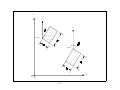
3-1. RELATIONSHIP OF AREA SOURCE PARAMETERS FOR ROTATED
RECTANGLE . . . . . . . . . . . . . . . . . . . . .
3-30
E-1. EXAMPLE OF AN ISC MESSAGE SUMMARY
ix
. . . . . . . . . . E-3
TABLES
Page
Table
3-1
3-2
SUMMARY OF SUGGESTED PROCEDURES FOR ESTIMATING
INITIAL LATERAL DIMENSIONS Fyo AND INITIAL VERTICAL
DIMENSIONS Fzo FOR VOLUME AND LINE SOURCES . . . . .
3-27
SURFACE ROUGHNESS LENGTH, METERS, FOR LAND-USE TYPES
AND SEASONS, FROM SHIEH ET AL., 1979 . . . . . . . .
3-89
B-1
DESCRIPTION OF CONTROL PATHWAY KEYWORDS
B-2
DESCRIPTION OF CONTROL PATHWAY KEYWORDS AND
PARAMETERS . . . . . . . . . . . . . . . . . . . . . . B-4
B-3
DESCRIPTION OF SOURCE PATHWAY KEYWORDS . . . . . . . . B-7
B-4
DESCRIPTION OF SOURCE PATHWAY KEYWORDS AND PARAMETERS
. . . . . . . . . . . . . . . . . . . . . . . . . . . B-8
B-5
DESCRIPTION OF RECEPTOR PATHWAY KEYWORDS . . . . . .
B-11
B-6
DESCRIPTION OF RECEPTOR PATHWAY KEYWORDS AND
PARAMETERS . . . . . . . . . . . . . . . . . . . . .
B-12
B-7
DESCRIPTION OF METEOROLOGY PATHWAY KEYWORDS
. . . .
B-15
B-8
DESCRIPTION OF METEOROLOGY PATHWAY KEYWORDS AND
PARAMETERS . . . . . . . . . . . . . . . . . . . . .
B-16
DESCRIPTION OF TERRAIN GRID PATHWAY KEYWORDS . . . .
B-19
B-10 DESCRIPTION OF TERRAIN GRID PATHWAY KEYWORDS AND
PARAMETERS . . . . . . . . . . . . . . . . . . . . .
B-20
B-11 DESCRIPTION OF EVENT PATHWAY KEYWORDS
. . . . . . .
B-21
B-12 DESCRIPTION OF EVENT PATHWAY KEYWORDS AND PARAMETERS
B-22
B-13 DESCRIPTION OF OUTPUT PATHWAY KEYWORDS . . . . . . .
B-23
B-9
. . . . . . . B-3
B-14 DESCRIPTION OF OUTPUT PATHWAY KEYWORDS AND PARAMETERS
. . . . . . . . . . . . . . . . . . . . . . . . . . B-24
x
1.0 INTRODUCTION
This section provides an overall introduction to the ISC
models and to the ISC User's Guide. It also serves
specifically as an introduction to the user instructions
contained in this volume for setting up and running the ISC
models. Some suggestions are offered on how various users
would best benefit from using the manuals. Also provided is an
overview of the model's applicability, range of options, basic
input data and hardware requirements, and a discussion of the
history of the ISC models. The input file needed to run the
ISC models is based on an approach that uses descriptive
keywords and allows for a flexible structure and format.
1.1 HOW TO USE THE ISC MANUALS
The ISC Model User's Guide has been designed in an attempt
to meet the needs of various types of users, depending on their
level of experience with the models. This section describes
briefly how different types of users would benefit most from
their use of the manual.
1.1.1 Novice Users
Novice users are those whose exposure to or experience
with the ISC models has been limited. They may be new to
dispersion modeling applications in general, or new to the ISC
models and therefore unfamiliar with the keyword/parameter
approach utilized for the input file. These users should
review the remainder of this Introduction to gain an overall
perspective of the use of ISC models, particularly for
regulatory modeling applications. They should then concentrate
their review on Section 2, which provides a brief tutorial on
setting up an input file that illustrates the most commonly
used options of the ISC Short Term model. Section 2 provides a
basic description of the input file structure and explains some
1-1
of the advantages of the keyword/parameter approach to
specifying modeling options and inputs. As the user becomes
more familiar with the operation of the models and encounters
the need to use more advanced features of the models, he/she
will want to review the contents of Section 3, which provides a
more detailed and complete reference of the various options for
running the models.
1.1.2 Experienced Modelers
Experienced modelers will have had considerable experience
in applying the ISC models in a variety of situations. They
should have basic familiarity with the overall goals and
purposes of regulatory modeling in general, and with the scope
of options available in the ISC models in particular.
Experienced modelers who are new to the ISC models will benefit
from first reviewing the contents of Section 2 of this volume,
which will give them a basic orientation to the structure,
organization and philosophy of the keyword/parameter approach
used for the input runstream file. Once they have a basic
grasp of the input file structure and syntax rules, they will
benefit most from using Section 3 of this volume as a reference
to learn the overall capabilities of the models, or to
understand the mechanics for implementing particular options.
The information in Section 3 is organized by pathway, with
detailed descriptions of each of the individual keyword options
by pathway. Once they are familiar with most or all of the
keywords, they may find the functional keyword reference
provided in Appendix B useful to quickly review the proper
syntax and available options/parameters for a particular
keyword. They may also find the Quick Reference available at
the end of the user's guide sufficient as a simple reminder of
the available keywords for each pathway and to ensure the
proper order of parameters for each input image.
1-2
Experienced modelers may also have occasion to peruse the
contents of Volume II, which describes the technical details of
the dispersion modeling algorithms utilized in the ISC models.
They may also have an interest in or need to review the
contents of Volume III to learn about the structure and
organization of the computer code, particularly if they are
involved with installing the code on another computer system,
or with compiling the code to meet the memory storage
requirements for a particular application.
1.1.3 Management/Decision Makers
Those involved in a management or decision-making role for
dispersion modeling applications will be especially interested
in the remainder of this section, which provides an overview of
the models, including their role in various regulatory
programs, a brief description of the range of available
options, and basic input data and computer hardware
requirements needed to run the models. From this information
they should understand the basic capabilities of the ISC models
well enough to judge the suitability of the models for
particular applications. They may also want to review the
brief tutorial provided in Section 2 to learn about the nature
and structure of the input runstream file, in order to better
be able to review the modeling results.
1.1.4 Programmers/Systems Analysts
Programmers and systems analysts, specifically those
involved with installing the ISC code on other computer systems
or charged with maintaining the code, should review the
contents of Volume III. This will acquaint them with the
structure and organization of the computer code, give specific
details on compiling and linking the code for various
situations, and explain in detail the memory storage
requirements and control of input and output (I/O). They may
1-3
also wish to review the remainder of this Introduction and the
brief tutorial in Section 2 of this volume in order to have a
basic understanding of the nature and overall capabilities of
the models, and to understand the basic input runstream file
structure and organization.
1.2 OVERVIEW OF THE ISC MODELS
This section provides an overview of the ISC models,
including a discussion of the regulatory applicability of the
models, a description of the basic options available for
running the models, and an explanation of the basic input data
and hardware requirements needed for executing the models.
1.2.1 Regulatory Applicability
The U.S. Environmental Protection Agency (EPA) maintains
the Guideline on Air Quality Models (Revised) (hereafter
referred to as the "Guideline"1) which provides the agency's
guidance on regulatory applicability of air quality dispersion
models in the review and preparation of new source permits and
State Implementation Plan (SIP) revisions. Regulatory
application of the ISC models should conform to the guidance
set forth in the Guideline, including the most recent
Supplements. Any non-guideline application of the models
should meet the requirements of the applicable reviewing
agency, such as an EPA Regional Office, a State or a local air
pollution control agency. In general, regulatory modeling
applications should be carried out in accordance with a
modeling protocol that is reviewed and approved by the
appropriate agency prior to conducting the modeling. The
modeling protocol should identify the specific model, modeling
options and input data to be used for a particular application.
1
The Guideline is published as Appendix W to 40 CFR Part 51.
1-4
1.2.2 Basic Input Data Requirements
There are two basic types of inputs that are needed to run
the ISC models. They are (1) the input runstream file, and (2)
the meteorological data file. The runstream setup file
contains the selected modeling options, as well as source
location and parameter data, receptor locations, meteorological
data file specifications, and output options. The ISC models
offer various options for file formats of the meteorological
data. These are described briefly later in this section, and
in more detail in Sections 2 and 3. A third type of input may
also be used by the models when implementing the dry deposition
and depletion algorithm. The user may optionally specify a
file of gridded terrain elevations that are used to integrate
the amount of plume material that has been depleted through dry
deposition processes along the path of the plume from the
source to the receptor. The optional terrain grid file is
described in more detail in Section 3. The user also has the
option of specifying a separate file of hourly emission rates
for the ISCST model.
1.2.3 Computer Hardware Requirements
1.2.3.1 PC Hardware Requirements.
Given the rapid increase in speed and capacity of personal
computers (PCs) available for modeling in recent years, and
their relative ease of use and access, the PC has become the
most popular environment for performing dispersion modeling
applications within the modeling community (Bauman and Dehart,
1988; Rorex, 1990). This trend can be expected to continue in
the future. The current versions of the ISC models were
developed on an IBM-compatible PC using the Microsoft FORTRAN
Optimizing Compiler (Version 5.1), and have been designed to
run on such machines with a minimum of 640K bytes of RAM and
MS-DOS Version 3.2 or higher. In order to handle the input
1-5
data files (runstream setup and meteorology) and the output
files, it is highly recommended that the system have a hard
disk drive. The amount of storage space required on the hard
disk for a particular application will depend greatly on the
output options selected. Some of the optional output files of
concentration data can be rather large. More information on
output file products is provided in Sections 2 and 3.
While a math coprocessor chip is optional for execution of
the ISC models on a PC, it is highly recommended, especially
for the Short Term model, due to the large increase in
execution speed that will be experienced. The model may be
expected to run about five to ten times faster with a math
coprocessor than without one.
For particularly large applications, involving a large
number of sources, source groups, receptors and averaging
periods, the user may find that the 640K RAM limit available
with DOS is not enough. In addition to the DOS executable
versions of the models, extended memory versions are available
for use on 80386, 80486 or higher PCs with at least 8 MB of RAM
for the ISCST model and at least 4 MB of RAM for the ISCLT
model. The extended memory versions of the models were
developed using the Lahey F77L/EM-32 Fortran Compiler (Version
5.2), and also require a math co-processor to be present. For
larger application scenarios, a Lahey-compiled ISCST executable
and 8 MB of RAM are recommended.
Section 4.2.2 of this volume
of the ISC User's Guide contains information on increasing the
capacity of the model and setting it up to run on systems (with
80386 processors and higher) that make use of extended memory
beyond the 640K limit of DOS. There are special requirements
for the operating system and Fortran language compiler needed
to utilize the extended memory on these machines.
1-6
1.2.3.2 DEC VAX Requirements.
The models have also been uploaded and tested on a DEC VAX
minicomputer. As with the IBM 3090, the VAX has some
advantages of speed and greater memory capacity over the PC
environment. There are no particular hardware requirements for
running the models on the VAX. The user must be familiar with
the operating system and Fortran language compiler being
utilized on the VAX in order to properly setup and run the
model and control the input and output files. Instructions for
setting up and running the models on the DEC VAX are included
in this volume and in more detail in Volume III of the User's
Guide.
1.2.3.3 IBM 3090 Requirements.
While the models were developed on the PC, they have been
uploaded and tested on EPA's IBM 3090 mainframe computer. The
mainframe has advantages of speed and greater memory capacity
over the PC environment. There are no particular hardware
requirements for running the models on the IBM 3090. However,
the user must be familiar with the IBM Job Control Language
(JCL) and the VS FORTRAN Version 2.0 compiler in order to
properly setup and run the models and control the input and
output files in the mainframe environment. Instructions for
setting up and running the models on the IBM 3090 are included
in this volume and in Volume III of the User's Guide.
1.2.4 Overview of Available Modeling Options
The ISC models include a wide range of options for
modeling air quality impacts of pollution sources, making them
popular choices among the modeling community for a variety of
applications. The following sections provide a brief overview
of the options available in the ISC models.
1-7
1.2.4.1 Dispersion Options.
Since the ISC models are especially designed to support
the EPA's regulatory modeling programs, the regulatory modeling
options, as specified in the Guideline on Air Quality Models
(Revised), are the default mode of operation for the models.
These options include the use of stack-tip downwash,
buoyancy-induced dispersion, final plume rise (except for
sources with building downwash), a routine for processing
averages when calm winds occur, default values for wind profile
exponents and for the vertical potential temperature gradients,
and the use of upper bound estimates for super-squat buildings
having an influence on the lateral dispersion of the plume. The
user can easily ensure the use of the regulatory default
options by selecting a single keyword on the modeling option
input card. To maintain the flexibility of the model, the
non-regulatory default options have been retained, and by using
descriptive keywords to specify these options it is evident at
a glance from the input or output file which options have been
employed for a particular application.
The Short Term model also incorporates the COMPLEX1
screening model dispersion algorithms for receptors in complex
terrain, i.e., where the receptor elevation is above the
release height of the source. The user has the option of
specifying only simple terrain (i.e., ISCST) calculations, only
complex terrain (i.e., COMPLEX1) calculations, or of using both
simple and complex terrain algorithms. In the latter case, the
model will select the higher of the simple and complex terrain
calculations on an hour-by-hour, source-by-source and receptorby-receptor basis for receptors in intermediate terrain, i.e.,
terrain between release height and plume height.
The user may select either rural or urban dispersion
parameters, depending on the characteristics of the source
location. The user also has the option of calculating
1-8
concentration values or deposition values for a particular run.
For the Short Term model, the user may select more than one
output type (concentration and/or deposition) in a single run,
depending on the setting for one of the array storage limits.
The user can specify several short term averages to be
calculated in a single run of the ISC Short Term model, as well
as requesting the overall period (e.g. annual) averages.
1.2.4.2 Source Options.
The model is capable of handling multiple sources,
including point, volume, area and open pit source types. Line
sources may also be modeled as a string of volume sources or as
elongated area sources. Several source groups may be specified
in a single run, with the source contributions combined for
each group. This is particularly useful for Prevention of
Significant Deterioration (PSD) applications where combined
impacts may be needed for a subset of the modeled background
sources that consume increment, while the combined impacts from
all background sources (and the permitted source) are needed to
demonstrate compliance with the National Ambient Air Quality
Standards (NAAQS). The models contain algorithms for modeling
the effects of aerodynamic downwash due to nearby buildings on
point source emissions, and algorithms for modeling the effects
of settling and removal (through dry deposition) of
particulates.
The Short Term model also contains an algorithm for
modeling the effects of precipitation scavenging for gases or
particulates. For the Short Term model, the user may specify
for the model to output dry deposition, wet deposition and/or
total deposition.
Source emission rates can be treated as constant
throughout the modeling period, or may be varied by month,
season, hour-of-day, or other optional periods of variation.
1-9
These variable emission rate factors may be specified for a
single source or for a group of sources. For the Short Term
model, the user may also specify a separate file of hourly
emission rates for some or all of the sources included in a
particular model run.
1.2.4.3 Receptor Options.
The ISC models have considerable flexibility in the
specification of receptor locations. The user has the
capability of specifying multiple receptor networks in a single
run, and may also mix Cartesian grid receptor networks and
polar grid receptor networks in the same run. This is useful
for applications where the user may need a coarse grid over the
whole modeling domain, but a denser grid in the area of maximum
expected impacts. There is also flexibility in specifying the
location of the origin for polar receptors, other than the
default origin at (0,0) in x,y, coordinates.
The user can input elevated receptor heights in order to
model the effects of terrain above (or below) stack base, and
may also specify receptor elevations above ground level to
model flagpole receptors. For simple terrain calculations, any
terrain heights input above the release height for a particular
source are "chopped-off" at the release height for that
source's calculations. The Short Term model includes the
complex terrain algorithms from the COMPLEX1 screening model.
If these algorithms are used, the model will calculate impacts
for terrain above the release height. The Long Term model does
not include any complex terrain algorithms.
1-10
1.2.4.4 Meteorology Options.
The Short Term model can utilize the unformatted,
sequential files of meteorological data generated by the
PCRAMMET and the MPRM preprocessors, provided the data file was
generated by the same Fortran compiler as was used for the
model, and provided the deposition algorithms are not being
used. The meteorology options for the deposition algorithms in
the ISC models are described later in this section.
The user also has considerable flexibility to utilize
formatted ASCII files that contain sequential hourly records of
meteorological variables. For these hourly ASCII files, the
user may use a default ASCII format, may specify the ASCII read
format, or may select free-formatted reads for inputting the
meteorological data. A utility program called BINTOASC is
provided with the ISC models to convert unformatted
meteorological data files of several types to the default ASCII
format used by ISCST and ISCEV. This greatly improves the
portability of applications to different computer systems. The
BINTOASC program is described in Appendix C. The model will
process all available meteorological data in the specified
input file by default, but the user can easily specify selected
days or ranges of days to process.
The Short Term model includes a dry deposition algorithm
and a wet deposition algorithm. The dry deposition algorithm
requires additional meteorological input variables, such as
Monin-Obukhov length and surface friction velocity, that are
provided by the PCRAMMET and MPRM preprocessor. The wet
deposition algorithm in the Short Term model also needs
precipitation data, which is optionally available in the
PCRAMMET preprocessed data. When using the dry deposition or
wet deposition algorithms in ISCST, the meteorological data
must be a formatted ASCII file.
1-11
The Long Term model uses joint frequency distributions of
wind speed class, by wind direction sector, by stability
category, known as STAR (STability ARray) summaries. These
STAR summaries are available from the National Climatic Data
Center in Asheville, North Carolina. They may also be
generated from sequential data files using the STAR utility
program available on EPA's SCRAM Bulletin Board System or by
the MPRM meteorological processor for on-site data. The
meteorological data for ISCLT are read in from a separate data
file, and the user may use a default ASCII format or may
specify the ASCII read format for the data.
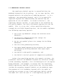
1.2.4.5 Output Options.
The basic types of printed output available with the Short
Term model are:
$
Summaries of high values (highest, second highest,
etc.) by receptor for each averaging period and source
group combination;
$
Summaries of overall maximum values (e.g., the maximum
50) for each averaging period and source group
combination; and
$
Tables of concurrent values summarized by receptor for
each averaging period and source group combination for
each day of data processed. These "raw" concentration
values may also be output to unformatted (binary)
files, as described below.
For the Long Term model, the user can also select output
tables of values for each receptor, and/or tables of overall
maximum values. The tables by receptor and maximum value
tables can be output for the source group values or for the
individual source values, or both. In addition, when maximum
values for individual sources are output, the user has the
option of specifying whether the values are to be the maximum
values for each source independently, or the contribution of
each source to the maximum group values, or both.
1-12
In addition to the tabular printed output products
described above, the ISC models provide options for several
types of file output products. One of these options for ISCST
is to output an unformatted ("binary") file of all
concentration and/or deposition values as they are calculated.
These files are often used for special postprocessing of the
data. In addition to the unformatted concentration files,
ISCST provides options for three additional types of file
outputs. One option is to generate an ASCII formatted file
with the same results that are included in the unformatted
postprocessing file. Another option is to generate a file of
(X,Y) coordinates and design values (e.g., the second highest
values at each receptor for a particular averaging period and
source group combination) that can be easily imported into many
graphics plotting packages to generate contour plots of the
concentration and/or deposition values. Separate files can be
specified for each of the averaging period and source group
combinations of interest to the user.
Another output file option of the ISCST model is to
generate a file of all occurrences when a concentration or
deposition value equals or exceeds a user-specified threshold.
Again, separate files are generated for only those combinations
of averaging period and source group that are of interest to
the user. These files include the date on which the threshold
exceedance occurred, the receptor location, and the
concentration value.
1.2.4.6 Source Contribution Analyses.
In air quality dispersion modeling applications, the user
may have a need to know the contribution that a particular
source makes to an overall concentration value for a group of
sources. This section provides a brief introduction to how
these types of source contribution (sometimes referred to as
source culpability) analyses are performed using the ISC
1-13
models. More detailed information about exercising these
options is provided in Section 3.
Recognizing that source contribution information is
important to many short term modeling analyses, the ISCST model
has been designed to facilitate performing this type of
analysis. This is accomplished with an additional model,
referred to as the ISC Short Term - EVENT model (ISCEV). The
ISCST model treats source groups independently. The ISCEV
(EVENT) model is set up specifically to provide the
contributions from individual sources to the concentration
values for particular events. These events may be the design
concentrations (e.g., the high-second-high 24-hour average
concentration for a particular group of sources) that were
generated from an execution of the ISCST model. Other events
of interest might be occurrences of violations of a particular
standard, for which it is necessary to determine whether the
source being permitted contributes above a significance level.
The models are set up in such a way that both of these types of
events can be passed directly from an execution of the ISCST
model to an input file for the EVENT model. The user is thus
able to run the models in a batch mode to obtain the overall
design value results from ISCST and the source contribution
information from ISCEV in a single step. The EVENT model can
also be run separately and accepts user-specified events for
source contribution processing.
In the ISCLT model, the user has an option to have the
highest 10 values for each source and source group reported
independently, or to have the 10 highest values from the
combined source group and the contributions from the individual
sources to those highest group values.
1-14
1.3 RELATION TO PREVIOUS VERSIONS OF ISC
1.3.1 Brief History of the ISC Models
The ISC3 models are based on revisions to the algorithms
contained in the ISC2 models. The latter came about as a
result of a major effort to restructure and reprogram the ISC
models that began in April 1989, and was completed in March
1992. The reprogramming effort was largely motivated by the
need to improve the quality, reliability, and maintainability
of the code when numerous "bugs" were discovered after the
implementation of the revised downwash algorithms for shorter
stacks. It became widely recognized that the code, originally
developed in the 1970's and modified numerous times since, had
become impossible to reliably modify, debug or maintain.
However, the goals of the reprogramming effort also included
improving the user interface by modifying the input file
structure and the output products, and to provide better "end
user" documentation for the revised models. The ISC2 models
were developed as replacements for and not updates to the
previous versions of the models.
1.3.2 Overview of New Features in the ISC3 Models
The ISC3 models include several new features. A revised
area source algorithm and revised dry deposition algorithm have
been incorporated in the models. The ISC3 models also include
an algorithm for modeling impacts of particulate emissions from
open pit sources, such as surface coal mines. The Short Term
model includes a new wet deposition algorithm, and also
incorporates the COMPLEX1 screening model algorithms for use
with complex and intermediate terrain. When both simple and
complex terrain algorithms are included in a Short Term model
run, the model will select the higher impact from the two
algorithms on an hour-by-hour, source-by-source, and receptorby-receptor basis for receptors located on intermediate
1-15
terrain, i.e., terrain located between the release height and
the plume height. A more detailed technical description of
these new features of the ISC models is included in Volume II
of the ISC User's Guide. The Long Term model does not include
wet deposition or complex terrain algorithms.
Some of the model input options have changed as a result
of the new features contained in the ISC3 models. There are
new options available on the CO MODELOPT card for both the
Short Term and Long Term models. The source deposition
parameters have changed somewhat with the new dry deposition
algorithm, and there are new source parameters needed for the
wet deposition algorithm in the Short Term model. Both models
include a new optional pathway for specifying a terrain grid
file that may be used in calculating the effects of plume
depletion due to dry removal mechanisms in elevated terrain.
There are also new meteorology input requirements for use of
the new deposition algorithms. The option for specifying
elevation units has been extended to source elevations and
terrain grid elevations, in addition to receptor elevations.
The CO ELEVUNIT card used to specify receptor elevations in the
previous version of ISC is now obsolescent, and is being
replaced by a new RE ELEVUNIT card. These new input options
are described in Section 3 and summarized in Appendix B.
The utility programs, STOLDNEW, BINTOASC, and METLIST,
described in Appendix C, have not been updated. While they may
continue to be used as before, they are not applicable to the
new deposition algorithms in the ISC3 models.
1-16
2.0 GETTING STARTED - A BRIEF TUTORIAL
This section provides a brief tutorial for setting up a
simple application problem with the ISC Short Term model, which
serves as an introduction for novice users to the ISC models.
The example illustrates the usage of the most commonly used
options in the ISC models for regulatory applications. A more
complete description of the available options for setting up
the ISC models is provided in Section 3.
The example problem presented in this section is a simple
application of the ISCST model to a single point source. The
source is a hypothetical stack at a small isolated facility in
a rural setting. Since the stack is below the Good Engineering
Practice (GEP) stack height, the emissions from the source are
subject to the influence of aerodynamic downwash due to the
presence of nearby buildings. The tutorial leads the user
through selection and specification of modeling options,
specification of source parameters, definition of receptor
locations, specification of the input meteorological data, and
selection of output options. Since this discussion is aimed at
novice users of the ISC models, a general description of the
input file keyword/parameter approach is provided first.
2.1 DESCRIPTION OF KEYWORD/PARAMETER APPROACH
The input file for the ISC models makes use of a
keyword/parameter approach to specifying the options and input
data for running the models. The descriptive keywords and
parameters that make up this input runstream file may be
thought of as a command language through which the user
communicates with the model what he/she wishes to accomplish
for a particular model run. The keywords specify the type of
option or input data being entered on each line of the input
file, and the parameters following the keyword define the
specific options selected or the actual input data. Some of
2-1
the parameters are also input as descriptive secondary
keywords.
The runstream file is divided into six functional
"pathways." These pathways are identified by a two-character
pathway ID placed at the beginning of each runstream image. The
pathways and the order in which they are input to the model are
as follows:
CO - for specifying overall job COntrol options;
SO - for specifying SOurce information;
RE - for specifying REceptor information;
ME - for specifying MEteorology information;
TG - for specifying Terrain Grid information; and
OU - for specifying OUtput options.
The TG pathway is an optional pathway that is only used for
implementing the dry depletion algorithm in elevated terrain.
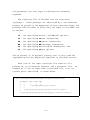
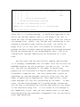
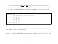
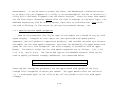
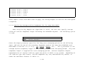
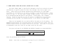
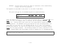
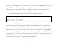
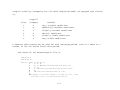
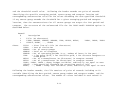
Each line of the input runstream file consists of a
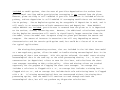
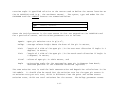
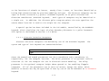
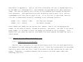
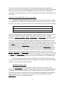
pathway ID, an 8-character keyword, and a parameter list. An
example of a line of input from a runstream file, with its
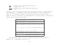
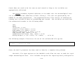
various parts identified, is shown below:
Column: 12345678901234567890123456789012345678901234567890123456789
CO MODELOPT DFAULT RURAL CONC
*
*
*
*
*
*
*
*
*
*
*
*
.))))))2)))))2))))))))) Parameters
*
*
*
.))))))))))))))))))))))))))))))))))) 8-Character Keyword
*
.)))))))))))))))))))))))))))))))))))))))))))) 2-Character Pathway ID
2-2
The following sections describe the rules for structuring
the input runstream file, and explain some of the advantages of
the keyword/parameter approach.
2.1.1 Basic Rules for Structuring Input Runstream Files
While the input runstream file has been designed to
provide the user with considerable flexibility in structuring
the input file, there are some basic syntax rules that need to
be followed. These rules serve to maintain some consistency
between input files generated by different users, to simplify
the job of error handling performed by the models on the input
data, and to provide information to the model in the
appropriate order wherever order is critical to the
interpretation of the inputs. These basic rules and the
various elements of the input runstream file are described in
the paragraphs that follow.
One of the most basic rules is that all inputs for a
particular pathway must be contiguous, i.e., all inputs for the
CO pathway must come first, followed by the inputs for the SO
pathway, and so on. The beginning of each pathway is
identified with a "STARTING" keyword, and the ending of the
pathway with the "FINISHED" keyword. Thus the first functional
record of each input file must be "CO STARTING" and the last
record of each input file must be "OU FINISHED." The rest of
the input images will define the options and input data for a
particular run.
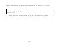
Each record in the input runstream file is referred to as
a runstream "image." These records are initially read into the
model as 132-character images. The information on each input
image consists of a "pathway," a "keyword," and one or more
"parameters." Each of these "fields" on the runstream image
must be separated from other fields by at least one blank
space. To simplify the interpretation of the runstream image
2-3
by the model, the runstream file must be structured with the
two-character pathway in columns 1 and 2, the eight-character
keyword in columns 4 through 11, followed by the parameters in
columns 13 through 132, as necessary. (For reasons that are
explained in Section 2.4.8, the models will accept input files
where all inputs are shifted by up to three columns to the
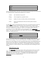
right.) For most keywords, the order of parameters following
the keyword is important -- the exact spacing of the parameters
is not important, as long as they are separated from each other
by at least one blank space and do not extend beyond the 132
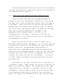
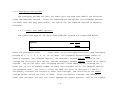
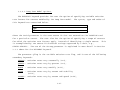
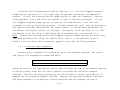
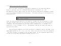
character limit. The example of a runstream image from the CO
pathway shown above is repeated here:
Column: 12345678901234567890123456789012345678901234567890123456789
CO MODELOPT DFAULT RURAL CONC
*
*
*
*
*
*
*
*
*
*
*
*
.))))))2)))))2))))))))) Parameters
*
*
*
.))))))))))))))))))))))))))))))))))) 8-Character Keyword
*
.)))))))))))))))))))))))))))))))))))))))))))) 2-Character Pathway ID
Alphabetical characters can be input as either lower case
or upper case letters. The models convert all character input
to upper case letters internally, with the exception of the
title fields and file names to be discussed later. Throughout
this document, the convention of using upper case letters is
followed. For numeric input data, it should be noted that all
data are assumed to be in metric units, i.e., length units of
meters, speed units of meters per second, temperature units of
degrees Kelvin, and emission units of grams per second. In a
few instances, the user has the option of specifying units of
feet for length and the model will perform the conversion to
meters. These exceptions are the input of receptor heights for
elevated terrain and the specification of anemometer height,
2-4
since these values are often more readily available in feet
than in meters.
Certain keywords are mandatory and must be present in
every runstream file, such as the MODELOPT keyword shown in the
example above which identifies the modeling options. Other
keywords are optional and are only needed to exercise
particular options, such as the option to allow for the input
of flagpole receptor heights. Some of the keywords are
repeatable, such as the keywords to specify source parameters,
while other keywords may only appear once. The keyword
references in Section 3, Appendices A and B and the Quick
Reference at the end of this volume identify each keyword as to
its type, either mandatory or optional, and either repeatable
or non-repeatable.
With a few exceptions that are described below, the order
of keywords within each pathway is not critical. For the CO
pathway, an exception is that the MODELOPT and POLLUTID
keywords must be specified before the DCAYCOEF or HALFLIFE
keyword because of the link between the urban default option
and the decay coefficient for SO2. For the SO pathway, the
LOCATION keyword must be specified before other keywords for a
particular source, and the SRCGROUP keyword must be the last
keyword before SO FINISHED. For keywords on the SO pathway
that accept a range of source IDs, the source parameters
specified by those keywords will only be applied to the sources
already defined, and will exclude any sources that are
specified latter in the input file.
2.1.2 Advantages of the Keyword Approach
The keyword approach provides some advantages over the
type of input file that uses non-descriptive numeric option
switches and requires rigidly formatted inputs. One advantage
is that the keywords are descriptive of the options and inputs
2-5
being used for a particular run, making it easier for a
reviewer to ascertain what was accomplished in a particular run
by reviewing the input file. Another advantage is that the
user has considerable flexibility in structuring the inputs to
improve their readability and understandability, as long as
they adhere to the few basic rules described above.
Some special provisions have been made to increase the
flexibility to the user in structuring the input files. One
provision is to allow for blank records in the input file.
This allows the user to separate the pathways from each other,
or to separate a group of images, such as source locations,
from the other images. Another provision is for the use of
"comment cards," identified by a "**" in the pathway field. Any
input image that has "**" for the pathway ID will be ignored by
the model. This is especially useful for labeling the columns
in the source parameter input images, as illustrated in the
example problem later in this section. It may also be used to
"comment out" certain options for a particular run without
deleting the options and associated data (e.g., elevated
terrain heights) completely from the input file. Because of
the descriptive nature of the keyword options and the
flexibility of the inputs it is generally much easier to make
modifications to an existing input runstream file to obtain the
desired result.
Another aspect of the "user-friendliness" of the ISC
models is that detailed error-handling has been built into the
models. The model provides descriptions of the location and
nature of all of the errors encountered for a particular run.
Rather than stopping execution at each occurrence of an input
error, the new model will read through and attempt to process
all input records and report all errors encountered. If a
fatal error occurs, then the model will not attempt to execute
the model calculations.
2-6
2.2 REGULATORY DEFAULT OPTION
The regulatory default option is controlled from the
MODELOPT keyword on the CO pathway. As its name implies, this
keyword controls the selection of modeling options. It is a
mandatory, non-repeatable keyword, and it is an especially
important keyword for understanding and controlling the
operation of the ISC models. As noted in Section 1, the
regulatory default options, as specified in the Guideline on
Air Quality Models, are truly the default options for the ISC
models. That is to say that, unless specified otherwise
through the available keyword options, the ISC models implement
the following regulatory options:
$
Use stack-tip downwash (except for Schulman-Scire
downwash);
$
Use buoyancy-induced dispersion (except for
Schulman-Scire downwash);
$
Do not use gradual plume rise (except for building
downwash);
$
Use the calms processing routines;
$
Use upper-bound concentration estimates for sources
influenced by building downwash from super-squat
buildings;
$
Use default wind profile exponents; and
$
Use default vertical potential temperature gradients.
Rather than specifying options with numeric switches, the
parameters used for the MODELOPT keyword are character strings,
called "secondary keywords," that are descriptive of the option
being selected. For example, to ensure that the regulatory
default options be used for a particular run, the user would
include the secondary keyword "DFAULT" on the MODELOPT input.
The presence of this secondary keyword tells the model to
override any attempt to use a non-regulatory default option.
The model will warn the user if a non-regulatory option is
2-7
selected along with the DFAULT option, but will not halt
processing. For regulatory modeling applications, it is
strongly suggested that the DFAULT switch be set, even though
the model defaults to the regulatory options without it.
For any application in which a non-regulatory option is to
be selected, the DFAULT switch must not be set, since it would
otherwise override the non-regulatory option. The
non-regulatory options are also specified by descriptive
secondary keywords, such as "NOBID" to specify the option not
to use buoyancy-induced dispersion. (A programmer note: these
modeling option keywords also correspond to the Fortran logical
variable names used to control the options in the ISC computer
code. This is one reason why they are limited to six
characters, .e.g., DFAULT instead of DEFAULT, since the
standard Fortran language (ANSI, 1978) only allows variable
names up to six characters in length).
The MODELOPT keyword, which is also used to specify the
selection of rural or urban dispersion parameters, and
concentration or deposition values, is described in more detail
in the Section 3.2.2.
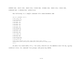
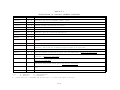
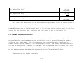
2.3 MODEL STORAGE LIMITS
The ISC models have been designed using a static storage
allocation approach, where the model results are stored in data
arrays, and the array limits are controlled by PARAMETER
statements in the Fortran computer code. These array limits
also correspond to the limits on the number of sources,
receptors, source groups and averaging periods that the model
can accept for a given run. Depending on the amount of memory
available on the particular computer system being used, and the
needs for a particular modeling application, the storage limits
can easily be changed by modifying the PARAMETER statements and
recompiling the model. Section 4.2.2 of this volume and Volume
2-8
III of the User's Guide provide more information about
modifying the storage limits of the models.
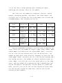
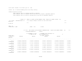
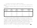
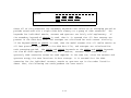
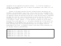
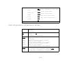
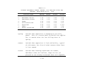
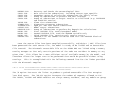
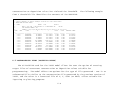
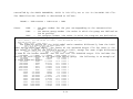
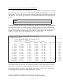
The limits on the number of receptors, sources, source
groups, averaging periods, and events (for ISCEV model) are
initially set as follows for the three models for the DOS and
extended memory (EM) versions on the PC:
PARAMETER
Name
Limit
Controlled
ISCST
ISCEV
ISCLT
NREC
Number of
Receptors
500 (DOS)
1200 (EM)
-
500 (DOS)
1200 (EM)
NSRC
Number of
Sources
100 (DOS)
300 (EM)
100 (DOS)
500 (EM)
50 (DOS)
300 (EM)
NGRP
Number of
Source
Groups
2 (DOS)
4 (EM)
25 (DOS)
50 (EM)
3 (DOS)
5 (EM)
NAVE
Number of
Short Term
Averages
2 (DOS)
4 (EM)
4 (DOS)
4 (EM)
-
NEVE
Number of
Events
-
2500 (DOS)
5000 (EM)
-
Fortran PARAMETER statements are also used to specify the
array limits for the number of output types (CONC, DEPOS, DDEP,
and/or WDEP) available with the ISCST model (NTYP, initially
set to 2 for the DOS version and 4 for the EM version); the
number of high short term values by receptor to store for the
ISCST model (NVAL, initially set to 2 for the DOS version and 6
for the EM version); the number of overall maximum values to
store (NMAX, initially set to 50 for ISCST and to 10 for Long
Term); and the number of x-coordinates and y-coordinates that
may be included in the optional terrain grid file (MXTX and
MXTY, initially set to 101 for the DOS version of Short Term,
201 for the DOS version of Long Term, and 601 for the EM
version of both models).
2-9
In addition to the parameters mentioned above, parameters
are used to specify the number of gridded receptor networks in
a particular run (NNET), and the number of x-coordinate (or
distance) and y-coordinate (or direction) values (IXM and IYM)
for each receptor network. Initially, the models allow up to 5
receptor networks (of any type), and up to 50 x-coordinates (or
distances) and up to 50 y-coordinates (or directions). The
source arrays also include limits on the number of variable
emission rate factors per source (NQF, initially set to 24 for
the DOS version of Short Term and 96 for the EM version of
Short Term, and to 36 for the DOS version of Long Term and 144
for the EM version of Long Term), the number of sectors for
direction-specific building dimensions (NSEC, initially set to
36 for Short Term and 16 for Long Term), and the number of
settling and removal categories (NPDMAX, initially set to 10
for the DOS version of Short Term and 20 for the EM version of
Short Term and both versions of Long Term).
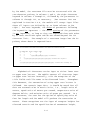
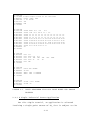
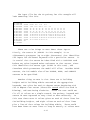
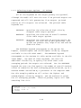
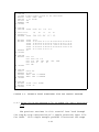
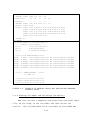
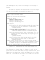
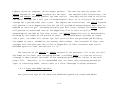
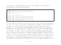
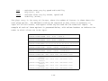
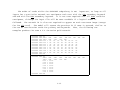
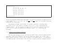
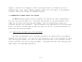
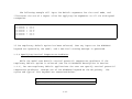
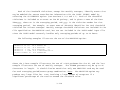
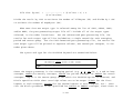
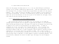
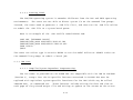
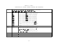
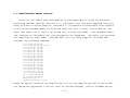
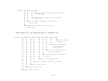
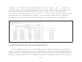
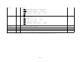
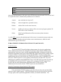
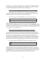
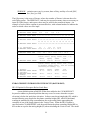
2.4 SETTING UP A SIMPLE RUNSTREAM FILE
This section goes through a step-by-step description of
setting up a simple application problem, illustrating the most
commonly used options of the ISCST model. The ISCST input
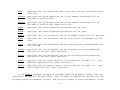
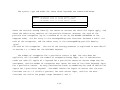
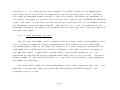
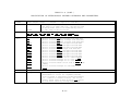
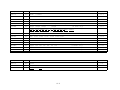
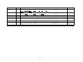
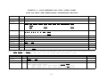
runstream file for the example problem is shown in Figure 2-1.
The remainder of this section explains the various parts of the
input file for the ISCST model, and also illustrates some of
the flexibility in structuring the input file.
2-10
CO
CO
CO
CO
CO
CO
CO
STARTING
TITLEONE A Simple Example Problem for the ISCST Model
MODELOPT DFAULT RURAL CONC
AVERTIME 3 24 PERIOD
POLLUTID SO2
RUNORNOT RUN
FINISHED
SO
SO
SO
SO
SO
SO
SO
SO
SO
SO
SO
SO
SO
STARTING
LOCATION
SRCPARAM
BUILDHGT
BUILDHGT
BUILDHGT
BUILDWID
BUILDWID
BUILDWID
BUILDWID
BUILDWID
SRCGROUP
FINISHED
STACK1
STACK1
STACK1
STACK1
STACK1
STACK1
STACK1
STACK1
STACK1
STACK1
ALL
RE
RE
RE
RE
RE
RE
RE
STARTING
GRIDPOLR
GRIDPOLR
GRIDPOLR
GRIDPOLR
GRIDPOLR
FINISHED
POL1
POL1
POL1
POL1
POL1
ME
ME
ME
ME
ME
ME
STARTING
INPUTFIL
ANEMHGHT
SURFDATA
UAIRDATA
FINISHED
PREPIT.BIN UNFORM
20 FEET
94823 1964 PITTSBURGH
94823 1964 PITTSBURGH
OU
OU
OU
OU
STARTING
RECTABLE
MAXTABLE
FINISHED
ALLAVE
ALLAVE
POINT 0.0
1.00 35.0
34. 34. 34.
34. 34. 34.
34. 34. 34.
35.43 36.45
15.00 20.56
35.43 33.33
25.50 20.56
36.37 36.45
STA
ORIG
DIST
GDIR
END
0.0
100.
36
FIRST
50
0.0
0.0
432.0 11.7
34. 34. 34.
34. 34. 34.
34. 34. 34.
36.37 35.18
25.50 29.66
35.43 36.45
15.00 20.56
35.43 33.33
0.0
200.
10.
300.
10.
2.4
34. 34. 34.
34. 34. 34.
34. 34. 34.
32.92 29.66
32.92 35.18
0.00 35.18
25.50 29.66
500.
34. 34. 34.
34. 34. 34.
34. 34. 34.
25.50 20.56
36.37 36.45
32.92 29.66
32.92 35.18
1000.
SECOND
FIGURE 2-1. INPUT RUNSTREAM FILE FOR ISCST MODEL FOR SAMPLE
PROBLEM
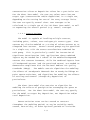
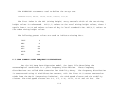
2.4.1 A Simple Industrial Source Application
For this simple tutorial, an application is selected
involving a single point source of SO2 that is subject to the
2-11
influences of building downwash. The source consists of a
35-meter stack with a buoyant release that is adjacent to a
building. We will assume that the stack is situated in a rural
setting with relatively flat terrain within 50 kilometers of
the plant. A polar receptor network will be placed around the
stack location to identify areas of maximum impact.
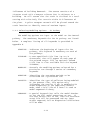
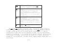
2.4.2 Selecting Modeling Options - CO Pathway
The modeling options are input to the model on the Control
pathway. The mandatory keywords for the CO pathway are listed
below. A complete listing of all keywords is provided in
Appendix B.
STARTING - Indicates the beginning of inputs for the
pathway; this keyword is mandatory on each of
the pathways.
TITLEONE - A user-specified title line (up to 68
characters) that will appear on each page of
the printed output file (an optional second
title line is also available with the keyword
TITLETWO).
MODELOPT - Controls the modeling options selected for a
particular run through a series of secondary
keywords.
AVERTIME - Identifies the averaging periods to be
calculated for a particular run.
POLLUTID - Identifies the type of pollutant being modeled.
At the present time, this option only
influences the results if SO2 is modeled with
urban dispersion in the regulatory default
mode, when a half-life of 4 hours is used to
model exponential decay.
RUNORNOT - A special keyword that tells the model whether
to run the full model executions or not. If
the user selects not to run, then the runstream
setup file will be processed and any input
errors reported, but no dispersion calculations
will be made.
2-12
FINISHED - Indicates that the user is finished with the
inputs for this pathway; this keyword is also
mandatory on each of the other pathways.
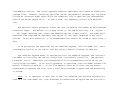
The first two keywords are fairly self-explanatory. As
discussed above in Section 2.2, the MODELOPT keyword on the CO
pathway is pivotal to controlling the modeling options used for
a particular run. For this example, we intend to use the
regulatory default options, so we will include the "DFAULT"
keyword on our MODELOPT input image. We also need to identify
whether the source being modeled is in a rural or an urban
environment (see Section 8.2.8 of the Guideline on Air Quality
Models for a discussion of rural/urban determinations). For
this example we are assuming that the facility is in a rural
setting. We also need to identify on this input image whether
we want the model to calculate concentration values or
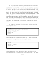
deposition values. For this example, we are calculating
concentration values. After the first three input records our
input file will look something like this:
CO STARTING
CO TITLEONE A Simple Example Problem for the ISCST Model
CO MODELOPT DFAULT RURAL CONC
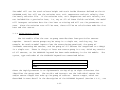
Note that the title parameter field does not need to be in
quotations, even though it represents a single parameter. The
model simply reads whatever appears in columns 13 through 80 of
the TITLEONE card as the title field, without changing the
lower case to upper case letters. Leading blanks are therefore
significant if the user wishes to center the title within the
field. Note also that the spacing and order of the secondary
2-13
keywords on the MODELOPT card are not significant.
card that looked like this:
CO MODELOPT
RURAL
CONC
A MODELOPT
DFAULT
would have an identical result as the example above. It is
suggested that the user adopt a style that is consistent and
easy to read. A complete description of the available modeling
options that can be specified on the MODELOPT keyword is
provided in Section 3.
Since the pollutant in this example is SO2, we will
probably need to calculate average values for 3-hour and
24-hour time periods, and we also need to calculate averages
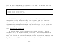
for the full annual time period. Our runstream file might
therefore look something like this after adding two more
keywords:
CO
CO
CO
CO
CO
STARTING
TITLEONE A Simple Example Problem for the ISCST Model
MODELOPT DFAULT RURAL CONC
AVERTIME 3 24 PERIOD
POLLUTID SO2
Note again that the order of the parameters on the AVERTIME
keyword is not critical, although the order of the short term
averages given on the AVERTIME keyword will also be the order
in which the results are presented in the output file. The
order of the keywords within each pathway is also not critical
in most cases, although the intent of the input runstream file
may be easier to decipher if a consistent and logical order is
followed. It is suggested that users follow the order in which
the keywords are presented in Section 3, in Appendix B, and in
the Quick Reference, unless there is a clear advantage to doing
otherwise.
2-14
The only remaining mandatory keywords for the CO pathway
are RUNORNOT and FINISHED. We will set the RUNORNOT switch to
RUN for this example. If a user is unsure about the operation
of certain options, or is setting up a complex runstream file
to run for the first time, it may be desirable to set the model
NOT to run, but simply to read and analyze the input file and
report any errors or warning messages that are generated. Once
the input file has been debugged using these descriptive
error/warning messages, then the RUNORNOT switch can be set to
RUN, avoiding a possible costly waste of resources generating
erroneous results. Even if the model is set NOT to run, all of
the inputs are summarized in the output file for the user to
review.
Our complete runstream file for the CO pathway may look
something like this:
CO
CO
CO
CO
CO
CO
CO
STARTING
TITLEONE A Simple Example Problem for the ISCST2 Model
MODELOPT DFAULT RURAL CONC
AVERTIME 3 24 PERIOD
POLLUTID SO2
RUNORNOT RUN
FINISHED
The following set of runstream images has a more structured
look, but it is equivalent to the example above:
CO STARTING
TITLEONE A Simple Example Problem for the ISCST2 Model
MODELOPT DFAULT RURAL CONC
AVERTIME 3 24 PERIOD
POLLUTID SO2
RUNORNOT RUN
CO FINISHED
Since the pathway ID is required to begin in column 1 (see
Section 2.4.8 for a discussion of this restriction), the model
2-15
will assume that the previous pathway is in effect if the
pathway field is left blank. The model will do the same for
blank keyword fields, which will be illustrated in the next
section.
In addition to these mandatory keywords on the CO pathway,
the user may select optional keywords to specify that elevated
terrain heights will be used (the default is flat terrain), to
allow the use of receptor heights above ground-level for
flagpole receptors, to specify a decay coefficient or a
half-life for exponential decay, and to generate an input file
containing events for processing with the EVENT model. The
user also has the option of having the model periodically save
the results to a file for later re-starting in the event of a
power failure or other interruption of the model's execution.
These options are described in more detail in Section 3 of this
volume.
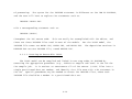
2.4.3 Specifying Source Inputs - SO Pathway
Besides the STARTING and FINISHED keywords that are
mandatory for all pathways, the Source pathway has the
following mandatory keywords:
LOCATION - Identifies a particular source ID and specifies
the source type and location of that source.
SRCPARAM - Specifies the source parameters for a
particular source ID identified by a previous
LOCATION card.
SRCGROUP - Specifies how sources will be grouped for
calculational purposes. There is always at
least one group, even though it may be the
group of ALL sources and even if there is only
one source.
Since the hypothetical source in our example problem is
influenced by a nearby building, we also need to include the
optional keywords BUILDHGT and BUILDWID in our input file.
2-16
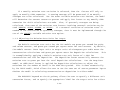
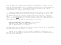
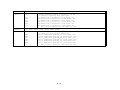
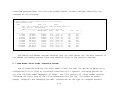
The input file for the SO pathway for this example will
look something like this:
SO
SO
SO
SO
SO
SO
SO
SO
SO
SO
SO
SO
SO
STARTING
LOCATION
SRCPARAM
BUILDHGT
BUILDHGT
BUILDHGT
BUILDWID
BUILDWID
BUILDWID
BUILDWID
BUILDWID
SRCGROUP
FINISHED
STACK1
STACK1
STACK1
STACK1
STACK1
STACK1
STACK1
STACK1
STACK1
STACK1
ALL
POINT 0.0
1.00 35.0
34. 34. 34.
34. 34. 34.
34. 34. 34.
35.43 36.45
15.00 20.56
35.43 33.33
25.50 20.56
36.37 36.45
0.0
0.0
432.0 11.7
34. 34. 34.
34. 34. 34.
34. 34. 34.
36.37 35.18
25.50 29.66
35.43 36.45
15.00 20.56
35.43 33.33
2.4
34. 34. 34.
34. 34. 34.
34. 34. 34.
32.92 29.66
32.92 35.18
0.00 35.18
25.50 29.66
34. 34. 34.
34. 34. 34.
34. 34. 34.
25.50 20.56
36.37 36.45
32.92 29.66
32.92 35.18
There are a few things to note about these inputs.
Firstly, the source ID (STACK1 in this example) is an
alphanumeric parameter (up to eight characters) that identifies
the inputs for different keywords with a particular source. It
is crucial that the source be identified with a LOCATION card
before any other keyword makes reference to that source, since
this identifies the source type (POINT in this case), and
therefore which parameters the model will allow. Besides POINT
sources, the ISC models also allow VOLUME, AREA, and OPENPIT
sources to be specified.
Another thing to note is that there are 36 building
heights and 36 building widths entered on the appropriate
keywords, one value for each 10 degree sector beginning with
the 10 degree flow vector (direction toward which the wind is
blowing), and continuing clockwise. Since the user could not
fit all 36 values on a single record, the pathway, keyword and
source ID were repeated as many times as were necessary. In
this case there were 12 values given on each of three lines for
the building heights, and eight values on each of four lines
plus a line of four values for building widths. There could
have been fewer or more lines as long as exactly 36 values were
2-17
entered before starting with a new keyword. Since all of the
building heights were the same across the sectors (fairly
realistic for the height but not for widths, unless the
structure was circular), there is a short cut available for
specifying numeric input in the runstream files for the new
models. The user can specify "repeat values" by entering a
field such as "36*34.0" as a parameter for the BUILDHGT
keyword. The model will interpret this as "36 separate
entries, each with a value of 34.0," and store the values in
the appropriate arrays within the model. Since the model must
identify this as a single parameter field, there must not be
any spaces between the repeat-value and the value to be
repeated.
The final keyword before finishing the SO pathway must be
the SRCGROUP keyword. In this example, since there is only one
source, we have taken advantage of a short cut provided by the
model by specifying a source group ID (which may be up to eight
characters) of ALL. Whenever this card appears in an input
file, it will generate a source group with a source-group ID of
ALL, consisting of all sources defined for that run. The
sources do not have to be explicitly identified. In a run
involving multiple sources, the user may specify multiple
source groups by repeating the SRCGROUP keyword. The use of
the SRCGROUP card is explained in more detail in Section 3.
2-18
Using some of the formatting options discussed above, the
SO pathway for our example may look like this, with the same
result as above:
SO STARTING
LOCATION
STACK1
** Point Source
** Parameters:
SRCPARAM STACK1
BUILDHGT
BUILDWID
SRCGROUP
SO FINISHED
STACK1
STACK1
STACK1
STACK1
STACK1
STACK1
ALL
POINT
QS
---1.00
0.0
0.0
0.0
HS
---35.0
TS
---432.
VS
---11.7
36.37
25.50
35.43
15.00
35.43
35.18 32.92 29.66 25.50 20.56
29.66 32.92 35.18 36.37 36.45
36.45 0.00 35.18 32.92 29.66
20.56 25.50 29.66 32.92 35.18
33.33
36*34.
35.43 36.45
15.00 20.56
35.43 33.33
25.50 20.56
36.37 36.45
DS
--2.4
This version of the SO pathway inputs illustrates the use of
the comment card to label the stack parameters on the SRCPARAM
card, i.e., QS for emission rate (g/s), HS for stack height
(m), TS for stack exit temperature (K), VS for exit velocity
(m/s), and DS for stack diameter (m). A complete description
of the source parameter card, with a list of parameters for
each source type, is provided in Section 3.3 and in Appendix B.
Other optional inputs that may be entered on the SO
pathway include specifying variable emission rate factors for
sources whose emissions vary as a function of month, season,
hour-of-day, STAR category, or season and hour-of-day (see
Section 3.3.4 for more details). The number of factors entered
depends on the option selected, and factors may be input for
single sources or for a range of sources. Other keywords allow
the user to specify settling velocity categories, mass
fractions, and reflection coefficients for sources of large
particulates that experience settling and removal of the
pollutant as it is dispersed and transported downwind. This
option is also explained in more detail in Section 3.
2-19
2.4.4 Specifying a Receptor Network - RE Pathway
As mentioned above, this example will illustrate the use
of a single polar receptor network centered on the stack
location. Other options available on the REceptor pathway
include specifying a Cartesian grid receptor network,
specifying discrete receptor locations in either a polar or a
Cartesian system, and specifying the location of receptors
along the boundary around a particular source. These other
options are described in more detail in Section 3.4.
For this example we will specify a polar network with
receptors located at five downwind distances for every
10-degree flow vector around the plant. There will be a total
of 180 receptors. The RE pathway for this example will look
something like this:
RE STARTING
GRIDPOLR
RE FINISHED
POL1
POL1
POL1
POL1
POL1
STA
ORIG
DIST
GDIR
END
0.0 0.0
100. 200.
36
10.
300.
10.
500.
1000.
The first thing to note about these inputs is that there
is a new set of keywords, including something that looks like a
STArting and ENDing. In fact the GRIDPOLR keyword can be
thought of as a "sub-pathway," in that all of the information
for a particular polar network must be in contiguous records,
and that the starting and ending of the sub-pathway are
identified. The order of secondary keywords within the
sub-pathway is not critical, similar to the main pathways. Each
card must be identified with a network ID (up to eight
alphanumeric characters), in this case it is "POL1." Multiple
networks may be specified in a single model run. The model
waits until the END secondary keyword is encountered to set the
2-20
variables, which may include terrain heights for receptors on
elevated terrain or flagpole receptor heights if those options
are being exercised by the user. The use of these optional
secondary keywords is described in detail in Section 3.4.
For this example, the ORIG secondary keyword specifies the
location of the origin, in (X,Y) coordinates, for the polar
network being defined. This network is centered at the same
(X,Y) location as the source specified above. The ORIG keyword
is optional, and the model will default to an origin of (0.0,
0.0) if it is omitted. The DIST keyword identifies the
distances along each direction radial at which the receptors
will be located. In this case there are five distances. More
could be added by adding values to that input card or by
including a continuation card, if needed. The GDIR keyword
specifies that the model will Generate DIRection radials for
the network, in this case there will be 36 directions,
beginning with the 10 degree flow vector and incrementing every
10 degrees clockwise. The user may elect to define Discrete
DIRection radials instead by using the DDIR keyword in place of
the GDIR keyword.
2.4.5 Specifying the Meteorological Input - ME Pathway
The MEteorolgy pathway has the following three mandatory
keywords (besides STARTING and FINISHED, of course):
INPUTFIL - Specifies the filename and format for the input
meteorological data file.
ANEMHGHT - Specifies the anemometer height for the wind
data to be used for the modeling run.
SURFDATA - Specifies information about the surface
meteorological data which will be used in the
modeling.
UAIRDATA - Specifies information about the upper air
meteorological data (i.e. mixing heights) which
will be used in the modeling.
2-21
For the purposes of this example we will assume that the
meteorological data file is a formatted ASCII file in the
default format for ISCST3 that was generated by the PCRAMMET
meteorological preprocessor program. The filename is
PREPIT.ASC (the sample file that is provided on the SCRAM BBS
with the ISCST3 model), and it consists of twenty days of data
for Pittsburgh, PA from 1964. The runstream images for the
MEteorology pathway would look something like this:
ME STARTING
INPUTFIL
ANEMHGHT
SURFDATA
UAIRDATA
ME FINISHED
PREPIT.ASC
20 FEET
94823 1964
94823 1964
PITTSBURGH
PITTSBURGH
The first parameter on the INPUTFIL keyword is the
filename, which can be entered as a full DOS pathname,
including the drive specification and subdirectories, up to a
total of 40 characters. The second parameter is the format of
the meteorology data file. In this case the secondary keyword
is blank, indicating that the meteorological data file is an
ASCII file in the default format for the model. Another option
would be to place the secondary keyword UNFORM following the
filename, in which case the model will assume an unformatted
meteorological data file of the type generated by PCRAMMET.
The order of variables assumed for the ASCII file input is as
follows: year, month, day, hour, flow vector, wind speed
(m/s), temperature (K), stability category, rural mixing height
(m), and urban mixing height (m). Other user options for
specifying the format for ASCII meteorology files are described
more fully in Section 3.5.1.
The ANEMHGHT keyword is important because the input wind
speed data are adjusted from the anemometer height to the
release height for model calculations, so that differences in
anemometer height can significantly effect the modeled results.
2-22
For National Weather Service (NWS) data, the user should check
records (e.g. the Local Climatological Data summary report) for
the particular station to determine the correct anemometer
height for the data period used in the modeling, since the
anemometer location and height may change over time. The model
will assume that the anemometer height is in meters, unless the
secondary keyword "FEET" is included in the runstream image, as
illustrated in this example. The model will convert inputs in
feet to meters.
The final two mandatory inputs identify the location and
data period of the input meteorological data. A separate
keyword is used for the surface meteorological data and for the
upper air (mixing height) data. The parameters on these cards
are the station number (e.g. WBAN number for NWS stations), the
data period (year), and a station name. It is important that
these inputs be provided correctly since the model compares the
station number and year from the runstream input file with
values provided in the first record of the meteorology file.
The user may also optionally input the (X,Y) coordinates for
the location of the station(s), although these values are not
currently used by the model.
Other optional keywords available on the ME pathway
provide the user with options to specify selected days to
process from the meteorological data file, a wind direction
rotation correction term, and user-specified wind speed profile
exponents and/or vertical potential temperature gradients. The
wind profile exponents and potential temperature gradients are
ignored (and a warning message generated) if the regulatory
default option is selected. These optional inputs are
described in more detail in Section 3.5.
2-23
2.4.6 Selecting Output Options - OU Pathway
All of the keywords on the Output pathway are optional,
although the model will warn the user if no printed outputs are
requested and will halt processing if no outputs (printed
results or file outputs) are selected. The printed table
keywords are:
RECTABLE - Specifies the selection of high value by
receptor table output options.
MAXTABLE - Specifies the selection of overall maximum
value table output options.
DAYTABLE - Specifies the selection of printed results (by
receptor) for each day of data processed (this
option can produce very large files and such be
used with care).
The RECTABLE keyword corresponds to the option for
highest, second-highest and third-highest values by receptor
available in the old ISCST model. The MAXTABLE keyword
corresponds to the maximum 50 table option available in the old
ISCST model. For both of these keywords, the user has
additional flexibility to specify for which short term
averaging periods the outputs are selected. For the MAXTABLE
keyword the user can also specify the number of overall maximum
values to summarize for each averaging period selected, up to a
maximum number controlled by a parameter in the computer code.
For this example problem we will select the highest and
second-highest values by receptor, and the maximum 50 values
for all averaging periods. These OU pathway inputs will look
something like this:
OU STARTING
RECTABLE
MAXTABLE
OU FINISHED
ALLAVE
ALLAVE
FIRST
50
SECOND
2-24
To simplify the input for users who request the same
printed table output options for all averaging periods, these
keywords recognize the secondary keyword "ALLAVE" as the first
parameter for that purpose. In order to obtain the overall
maximum 10 values for the 24-hour averages only, then the OU
pathway images would look like this:
OU STARTING
RECTABLE
MAXTABLE
OU FINISHED
ALLAVE
24 10
FIRST
SECOND
It should also be noted that these output table options apply
only to the short-term averaging periods, such as the 3-hour
and 24-hour averages used in our example. If the user has
selected that PERIOD averages be calculated (on the CO AVERTIME
keyword), then the output file will automatically include a
table of period averages summarized by receptor (the RECTABLE
option does not apply since there is only one period value for
each receptor). In addition, the printed output file will
include tables summarizing the highest values for each
averaging period and source group.
Other options on the OU pathway include several keywords
to produce output files for specialized purposes, such as
generating contour plots of high values, identifying
occurrences of violations of a particular threshold value (e.g.
a NAAQS), and for postprocessing of the raw concentration data.
These options are described in detail in Section 3.6.
The complete input runstream file for this simple example
is shown in Figure 2-2. Note that a consistent style has been
used for formatting and structuring the file in order to
improve its readability. This input file is comparable to the
version shown earlier in Figure 2-1, which used a somewhat
different style.
2-25
CO STARTING
TITLEONE A Simple Example Problem for the ISCST2 Model
MODELOPT DFAULT RURAL CONC
AVERTIME 3 24 PERIOD
POLLUTID SO2
RUNORNOT RUN
CO FINISHED
SO STARTING
LOCATION
STACK1
** Point Source
** Parameters:
SRCPARAM STACK1
BUILDHGT
BUILDWID
SRCGROUP
SO FINISHED
RE STARTING
GRIDPOLR
RE FINISHED
STACK1
STACK1
STACK1
STACK1
STACK1
STACK1
ALL
POL1
POL1
POL1
POL1
POL1
POINT
QS
---1.00
0.0
0.0
0.0
HS
---35.0
TS
---432.
VS
---11.7
36.37
25.50
35.43
15.00
35.43
35.18 32.92 29.66 25.50 20.56
29.66 32.92 35.18 36.37 36.45
36.45 0.00 35.18 32.92 29.66
20.56 25.50 29.66 32.92 35.18
33.33
36*34.
35.43 36.45
15.00 20.56
35.43 33.33
25.50 20.56
36.37 36.45
STA
ORIG
DIST
GDIR
END
ME STARTING
INPUTFIL
ANEMHGHT
SURFDATA
UAIRDATA
ME FINISHED
PREPIT.ASC
20 FEET
94823 1964
94823 1964
OU STARTING
RECTABLE
MAXTABLE
OU FINISHED
ALLAVE
ALLAVE
0.0 0.0
100. 200.
36
10.
FIRST
50
300.
10.
DS
--2.4
500.
1000.
PITTSBURGH
PITTSBURGH
SECOND
FIGURE 2-2. EXAMPLE INPUT RUNSTREAM FILE FOR SAMPLE PROBLEM
2.4.7 Using the Error Message File to Debug the Input Runstream
File
The previous sections in this tutorial have lead through
the step-by-step construction of a sample runstream input file
for ISCST. This simple example problem illustrated the usage
2-26
of the most commonly used options of the ISCST model. However,
many real-time applications of the model will be much more
complex than this example, perhaps involving multiple sources
and source groups, multiple receptor networks, the addition of
discrete receptor locations, and/or elevated terrain heights.
Since humans are prone to make errors from time to time, an
effort has been made to develop improved error handling
capabilities for the ISC models.
The error handling capabilities of the ISC models are
designed to accomplish two things for the user. First, the
model should read through the complete input file and report
all occurrences of errors or suspect entries before stopping,
rather than stopping on the first instance (and every instance
thereafter) of an error in the input file. Second, the model
should provide error and warning messages that are detailed and
descriptive enough that they will help the user in his/her
effort to debug the input file. The remainder of this section
provides of brief introduction to the use of the model's error
handling capabilities. Appendix E of this volume provides more
details about the error handling provided by the ISC models,
including a listing and explanation of all error and other
types of messages generated by the models.
The ISC models generate messages during the processing of
the input data and during the execution of model calculations.
These messages inform the user about a range of possible
conditions including:
$
Errors that will halt any further processing, except to
identify additional error conditions;
$
Warnings that do not halt processing but indicate a
possible errors or suspect conditions; and
$
Informational messages that may be of interest to the
user but have no direct bearing on the validity of the
results.
2-27
As the model encounters a condition for which a message is
generated, the model writes the message to a temporary storage
file. At the completion of the setup processing for a run, and
at the completion of the model calculations, the model rereads
the message file and generates a summary of the messages which
is included in the main printed output file. If the processing
of the model setup information indicates no errors or warnings,
and the user has selected the option to RUN the model
calculations on the CO RUNORNOT card, then the model will
simply write a statement to the print file that the model setup
was completed successfully. Otherwise, the model will report a
summary of the messages encountered. The summary of model
setup messages that would be generated for the example problem
if the option NOT to run was chosen is shown in Figure 2-3.
This summary table reports the total number of occurrences for
each of the message types, and lists the detailed message for
any fatal errors or warning messages that were generated. In
this case, since there were no errors or suspicious conditions
in the setup file, there are no error or warning messages
listed.
An example of the warning message that would have been
generated had we left out the card on the RE pathway that
specifies the origin of the polar receptor network is shown
below:
2-28
RE W220 39 REPOLR: Missing Origin (Use Default = 0,0) In GRIDPOLR
POL1
*
*
*
*
*
*
*
*
*
*
*
*
Hints
*
*
*
*
*
*
*
*
*
*
Detailed error/warning message
*
*
*
*
*
*
*
*
*
* Subroutine from which message is generated
*
*
*
*
* Line number of file where message occurred
*
*
*
* Message code - including message type (E, W, I) and message number
*
Pathway ID where message originated
Since this is a warning message, it would have appeared at the
end of the message summary table in the output file, but it
would not have halted processing of the data. The last item on
the message line, "Hints," may include such information as the
keyword or parameter name causing the error, the source ID,
group ID or (as in this case) the network ID involved, or
perhaps the date variable identifying when the message occurred
during the processing of the meteorological data, such as an
informational message identifying the occurrence of a calm
wind.
For new users and for particularly complex applications,
it is strongly recommended that the model first be run with the
RUNORNOT keyword (on the CO pathway) set NOT to run. In this
way, the user can determine if the model is being setup
properly by the runstream file before committing the resources
to perform a complete run. The user should make a point of
examining any warning messages carefully to be sure that the
model is operating as expected for their application, since
these messages will not halt processing by the model. In most
cases, the detailed messages will provide enough information
for the user to determine the location and nature of any errors
in the runstream setup file. If the intent of the message is
not immediately clear, then the user should refer to the more
detailed descriptions provided in Appendix E for the particular
error code generated.
2-29
In deciphering the error and warning messages, the line
number provided as part of the message may be particularly
helpful in locating the error within the input file. However,
if it is an error of omission that is caught by the error
checking performed at the completion of inputs for a pathway,
then the line number will correspond to the last record for
that pathway. The user may need to examine all of the messages
carefully before locating the error or errors, especially since
a single occurrence of certain types of errors may lead to
other error conditions being identified later in the input file
which do not really constitute errors in themselves. An
example of this is provided in Figure 2-4, which shows some
inputs for the SO pathway where the building dimension keywords
have been typed incorrectly, and the associated list of error
messages. Since continuation cards were being used for the
building width inputs, and the keyword was entered incorrectly
on the first line, the subsequent records were also taken by
the model to be invalid keyword inputs. While the error
messages are the same for these records, the message originates
from a different part of the model (SUBROUTINE SOCARD) for the
records with the blank keyword.
Since the detailed error and warning messages are listed
in the output file as part of the message summary table, there
will generally not be a need for the user to examine the
contents of the detailed message file. For this reason, the
default operation of the model is to write the messages that
are generated by a particular run to a temporary file that is
deleted when the run is completed. If the user wishes to
examine the complete list of detailed messages (of all types),
there is an optional keyword available on the CO pathway for
that purpose. The ERRORFIL keyword, which is described in
2-30
detail in Section 3.2.7, allows the user to save the complete
list of detailed messages to a user-specified filename.
*** Message Summary For ISC3 Model Setup ***
--------- Summary of Total Messages --------A Total of
A Total of
A Total of
0 Fatal Error Message(s)
0 Warning Message(s)
0 Information Message(s)
******** FATAL ERROR MESSAGES ********
*** NONE ***
********
WARNING MESSAGES
*** NONE ***
********
***********************************
*** SETUP Finishes Successfully ***
***********************************
FIGURE 2-3.
EXAMPLE MESSAGE SUMMARY TABLE FOR RUNSTREAM SETUP
2-31
SO STARTING
LOCATION
STACK1
0.0
0.0
QS
HS
TS
VS
** Parameters:
----
----
----
----
---
SRCPARAM
STACK1
1.00
35.0
432.0
11.7
2.4
BUILDHTS
STACK1
36*34.
BUILDWTS
STACK1
35.43 36.45 36.37 35.18 32.92 29.66 25.50 20.56
STACK1
15.00 20.56 25.50 29.66 32.92 35.18 36.37 36.45
STACK1
35.43 33.33 35.43 36.45
STACK1
25.50 20.56 15.00 20.56 25.50 29.66 32.92 35.18
STACK1
36.37 36.45 35.43 33.33
** Point Source
SRCGROUP
POINT
0.0
DS
0.00 35.18 32.92 29.66
ALL
SO FINISHED
*** Message Summary For ISC3 Model Setup ***
--------- Summary of Total Messages --------A Total of
6 Fatal Error Message(s)
A Total of
0 Warning Message(s)
A Total of
0 Information Message(s)
******** FATAL ERROR MESSAGES ********
SO E105
17 EXKEY : Invalid Keyword Specified. The Troubled Keyword is BUILDHTS
SO E105
18 EXKEY : Invalid Keyword Specified. The Troubled Keyword is BUILDWTS
SO E105
19 SOCARD: Invalid Keyword Specified. The Troubled Keyword is BUILDWTS
SO E105
20 SOCARD: Invalid Keyword Specified. The Troubled Keyword is BUILDWTS
SO E105
21 SOCARD: Invalid Keyword Specified. The Troubled Keyword is BUILDWTS
SO E105
22 SOCARD: Invalid Keyword Specified. The Troubled Keyword is BUILDWTS
********
WARNING MESSAGES
***
NONE
********
***
**************************************
*** SETUP Finishes UN-successfully ***
**************************************
FIGURE 2-4. EXAMPLE OF KEYWORD ERROR AND ASSOCIATED MESSAGE
SUMMARY TABLE
2.4.8 Running the Model and Reviewing the Results
Now that we have a complete and error-free runstream input
file, we are ready to run the model and then review the
results. The PC-executable files available on the SCRAM BBS
2-32
open the runstream input and printed output files explicitly
within the model, so there is no need to "redirect" the I/O on
the command line using the DOS redirection symbols '<' and '>'.
The command line to run the sample problem might look something
like this on the PC:
C:\>ISCST3 TEST-ST.INP TEST-ST.OUT
The "c-prompt" of DOS has been represented by the characters
"C:\>", but may appear different on different machines. The
important points are that the ISCST3.EXE file either be in the
directory from which you are attempting to run the model, or in
a directory that is included on the DOS PATH command when the
system is "booted-up." The runstream input filename must
appear first (without any DOS "redirection" symbol), followed
by the desired output filename (also without the DOS
redirection symbol), and these files must also be located in
the directory from which the model is being executed, unless a
complete DOS pathname is provided on the command line.
As mentioned above, the SCRAM PC-executable files for ISC
open the input and output files explicitly. One reason for
this is to allow for the models to write an update on the
status of processing to the PC terminal screen. For the ISCST
model, the model first indicates that setup information is
being processed and then gives the Julian day currently being
processed. If no status message is seen then the model did not
load into memory properly. If the model stops after completing
the setup processing, then either the RUNORNOT option was set
NOT to run, or a fatal error was encountered during the setup
processing. Another reason for not sending the printed output
to the default output device (i.e., to the screen or redirected
to a file), is so that any DOS error messages will be visible
on the screen and not be written to the printed file. One such
message might be that there is insufficient memory available to
run the program. Handling of DOS error messages may require
2-33
some knowledge of DOS, unless the meaning of the message is
obvious.
The order of contents and organization of the main output
file for the ISC models is presented in Figure 2-5.
Echo of Input Runstream Images
Summary of Runstream Setup Messages
Summary of Inputs
Summary of Modeling Options
Summary of Source Data
Summary of Receptor Data
Summary of Meteorology Data
Model Results
Daily Results for Each Averaging Period and Output Type
Selected for Each Day Processed (If Applicable)
- DAYTABLE Keyword
PERIOD or ANNUAL Results for Each Source Group and
Output Type (If Applicable)
- PERIOD or ANNUAL Parameter on AVERTIME Keyword
Short Term Average Results (High, Second High, etc.) by
Receptor for Each Source Group and Output Type (If
Applicable)
- RECTABLE Keyword
Overall Maximum Short Term Average Results for Each
Source Group and Output Type (If Applicable)
- MAXTABLE Keyword
Summary Tables of High Values for Each Averaging Period,
Source Group and Output Type (Always provided if PERIOD
or ANNUAL averages or the RECTABLE keyword are used)
Summary of Complete Model Execution Messages
FIGURE 2-5.
ORGANIZATION OF ISCST MODEL OUTPUT FILE
The references to "Output Type" in Figure 2-5 refer to the
option with the Short Term model to output concentration, total
deposition, dry deposition, and/or wet deposition in a single
model run. Each page of the output file, except for the echo
2-34
of the input file images, is labeled with the model name and
version number, user-specified title(s), page number, and, for
the PC version of the model, the date and time of the
particular run. Also included as part of the header
information for each page is a one-line summary of the modeling
options used for that particular run. The modeling options are
listed as the secondary keywords used to control the options,
such as URBAN or RURAL, CONC or DEPOS, DFAULT, NOCALM, etc.
(Details about the date/time routines and other PC-specific
features of the computer code are discussed in Section 4.0 of
this Volume and in Volume III.)
Since the complete input file is normally echoed back as
part of the output file, and since processing of the inputs
stops when the OU FINISHED card is reached, the run can be
duplicated by simply specifying the output filename as the
input runstream file. Alternatively, the input records could
be "cut and pasted" from the output file to a separate file
using a text editor. This allows for the model run to be
duplicated even if the original runstream file is not
available.
By default, the models will echo each line of the input
runstream file to the printed output file. This provides a
convenient record of the inputs as originally read into the
model, without any rounding of numerical values that may appear
in the input summary tables. As noted above, it also means
that the output file can be used as an input file to the model
to reproduce a particular application. However, for some
applications, the length of the input runstream file may be too
cumbersome to include the entire set of inputs at the beginning
of each output file. This may happen, for example, if a large
number of sources are being defined or if a large number of
discrete receptor locations are used. For this reason, the
user is provided with the option to "turn off" the echoing of
the input file at any point within the runstream file. This is
2-35
accomplished by entering the keywords "NO ECHO" in the first
two fields anywhere within the runstream file. In other words,
place NO in the pathway field, followed by a space and then
ECHO. None of the input runstream images after the NO ECHO
will be echoed to the output file. Thus, a user may choose to
place NO ECHO after the Control pathway in order to keep the
control options echoed, but suppress echoing the rest of the
input file.
The details of the message summary tables were discussed
in the previous section. A portion of the summary of modeling
option inputs is shown in Figure 2-6 for the simple example
described in this section. For the new model, the summary of
source parameter input data includes separate tables for each
source type, rather than combining all sources onto a single
table. In this way the column headings are specific to the
source type.
Figure 2-7 presents an example of the results output for
the second highest values by receptor for our sample problem.
These values are the second highest 24-hour averages at each
receptor location. Note that several of the numbers are
followed by a 'c.' This flag indicates that the average
included at least one calm hour during the averaging period.
The number in parentheses following each concentration value is
the date corresponding to each value. The date is given as an
eight digit integer variable that includes the year (2-digits),
month, day, and hour corresponding to the end of the averaging
period. Since these are 24-hour averages and are based on
block (end-to-end) rather than running averages, all of the
dates end on hour 24.
For each of the different types of model result tables,
the controlling keyword is identified above at the end of the
description. All of the outputs of the same type, e.g. high
values by receptor, are printed together, and the order of
2-36
tables loops through all source groups for a particular
averaging period, and then loops through all averaging periods.
The summary tables of high values at the end of the model
results follow the same order of loops. An example of the
summary tables for our sample problem is shown in Figure 2-8.
The summaries for all averaging periods have been combined onto
a single figure, but would appear on separate pages of the
actual output file.
2-37
*** ISCST3 - VERSION 95250 ***
09/07/95
12:00:00
*** A Simple Example Problem for the ISCST Model
***
***
***
PAGE
1
**MODELOPTs: CONC
RURAL
FLAT
DFAULT
***
MODEL SETUP OPTIONS SUMMARY
***
- - - - - - - - - - - - - - - - - - - - - - - - - - - - - - - - - - - - - - - - - - - - - - - - - - - - - - - - - - - - - **Intermediate Terrain Processing is Selected
**Model Is Setup For Calculation of Average CONCentration Values.
-- SCAVENGING/DEPOSITION LOGIC -**Model Uses NO DRY DEPLETION. DDPLETE = F
**Model Uses NO WET DEPLETION. WDPLETE = F
**NO WET SCAVENGING Data Provided.
**Model Does NOT Use GRIDDED TERRAIN Data for Depletion Calculations
**Model Uses RURAL Dispersion.
**Model Uses Regulatory DEFAULT Options:
1. Final Plume Rise.
2. Stack-tip Downwash.
3. Buoyancy-induced Dispersion.
4. Use Calms Processing Routine.
5. Not Use Missing Data Processing Routine.
6. Default Wind Profile Exponents.
7. Default Vertical Potential Temperature Gradients.
8. "Upper Bound" Values for Supersquat Buildings.
9. No Exponential Decay for RURAL Mode
**Model Assumes Receptors on FLAT Terrain.
**Model Assumes No FLAGPOLE Receptor Heights.
**Model Calculates 2 Short Term Average(s) of:
and Calculates PERIOD Averages
**This Run Includes:
1 Source(s);
3-HR
24-HR
1 Source Group(s); and
2-38
180 Receptor(s)
**The Model Assumes A Pollutant Type of:
SO2
**Model Set To Continue RUNning After the Setup Testing.
**Output Options Selected:
Model Outputs Tables of PERIOD Averages by Receptor
Model Outputs Tables of Highest Short Term Values by Receptor (RECTABLE Keyword)
Model Outputs Tables of Overall Maximum Short Term Values (MAXTABLE Keyword)
FIGURE 2-6.
*** ISCST3 - VERSION 95250 ***
09/07/95
12:00:30
PAGE 13
**MODELOPTs: CONC
SAMPLE OF MODEL OPTION SUMMARY TABLE FROM AN ISC MODEL OUTPUT FILE
*** A Simple Example Problem for the ISCST Model
***
***
***
RURAL
FLAT
DFAULT
*** THE
2ND HIGHEST 24-HR AVERAGE CONCENTRATION
INCLUDING SOURCE(S):
STACK1 ,
*** NETWORK ID: POL1
** CONC OF SO2
VALUES FOR SOURCE GROUP:
; NETWORK TYPE: GRIDPOLR ***
IN MICROGRAMS/M**3
DISTANCE (METERS)
300.00
ALL
***
**
DIRECTION |
(DEGREES) |
100.00
200.00
500.00
1000.00
- - - - - - - - - - - - - - - - - - - - - - - - - - - - - - - - - - - - - - - - - - - - - - - - - - - - - - - - - - - - - - - - 10.0 |
0.00038 (64010524)
0.00759 (64010324)
0.00223 (64010224)
0.00058 (64010224)
0.00012
(64010224)
20.0 |
0.00032 (64010224)
0.73597 (64010324)
0.46271 (64010324)
0.22714 (64010324)
0.08851
(64010324)
30.0 |
0.06544 (64010324)
3.09471 (64010224)
2.05010 (64010224)
1.00969 (64010224)
0.46573
(64010224)
40.0 |
2.24546 (64010524)
7.13027 (64010324)
4.90821 (64010324)
2.56813 (64010524)
1.20217
(64010524)
50.0 |
17.05618 (64010524)
12.96035 (64010524)
8.87260 (64010524)
4.40116 (64010524)
2.17334
(64010524)
60.0 |
9.40921 (64010224)
6.06938 (64010224)
4.17845 (64010224)
2.05521 (64010224)
0.94001
(64010224)
2-39
70.0 |
4.98424 (64011024)
(64011024)
80.0 |
1.10668 (64010424)
(64010124)
90.0 |
0.33531 (64010424)
(64011024)
100.0 |
1.14289 (64011024)
(64011024)
110.0 |
1.38580 (64010424)
(64010424)
120.0 |
1.46832c(64010724)
0.06649c(64010724)
130.0 |
0.73820 (64010924)
(64010924)
140.0 |
0.00385 (64010924)
(64010924)
150.0 |
0.00000 (64010924)
(64010124)
160.0 |
0.00000 (64010924)
(64010124)
170.0 |
0.00000 (
0)
(64010124)
180.0 |
0.00000 (
0)
(64010124)
190.0 |
0.00000 (64010124)
(64010124)
200.0 |
0.00000 (64010124)
(64010124)
210.0 |
0.00000c(64010724)
0.00315c(64010724)
220.0 |
0.00000c(64010724)
0.00000c(64010724)
230.0 |
0.00017 (64010824)
(64010824)
240.0 |
0.82936 (64010824)
(64010824)
250.0 |
2.85290 (64010124)
(64010824)
260.0 |
0.93134 (64010824)
(64010824)
270.0 |
0.01273 (64010824)
(64010824)
280.0 |
0.44666 (64010924)
(64010924)
4.83446 (64011024)
3.64057 (64011024)
1.93861 (64011024)
0.96955
1.32557 (64010124)
0.99239 (64010124)
0.55702 (64010124)
0.38055
0.89549 (64010424)
0.76865 (64010424)
0.55710 (64010424)
0.68970
1.66369 (64011024)
1.30464 (64011024)
0.77602 (64010924)
0.45574
1.41520 (64010424)
1.09491 (64010424)
0.59547 (64010424)
0.32417
0.72598c(64010724)
0.41049c(64010724)
0.12771c(64010724)
0.50974 (64010924)
0.36027 (64010924)
0.16093 (64010924)
0.07651
0.00152 (64010924)
0.00072 (64010924)
0.00020 (64010924)
0.00004
0.00000 (64010124)
0.00000 (64010124)
0.00000 (64010124)
0.00000
0.00203 (64010124)
0.00054 (64010124)
0.00005 (64010124)
0.00003
0.12191 (64010124)
0.04290 (64010124)
0.00504 (64010124)
0.00702
0.04481 (64010124)
0.01473 (64010124)
0.00161 (64010124)
0.00183
0.00008 (64010124)
0.00002 (64010124)
0.00000 (64010124)
0.00000
0.00000 (64010124)
0.00000 (64010124)
0.00003 (64010124)
0.00087
0.00014 (64010124)
0.00003 (64010124)
0.00020 (64010124)
0.00021c(64010724)
0.00005c(64010724)
0.00000c(64010724)
0.00004 (64010824)
0.00001 (64010824)
0.00000 (64010824)
0.00000
0.52206 (64010824)
0.34721 (64010824)
0.10982 (64010824)
0.06490
2.16804 (64010124)
1.36673 (64010824)
0.46188 (64010824)
0.34731
0.90262 (64010824)
0.43338 (64010824)
0.15206 (64010824)
0.12491
0.02553 (64010824)
0.02055 (64010824)
0.01631 (64010824)
0.05295
0.36178 (64010924)
0.24921 (64010924)
0.10171 (64010924)
0.05489
2-40
290.0 |
1.99281 (64010924)
(64010924)
300.0 |
3.26315 (64010924)
(64010924)
310.0 |
1.61856 (64010824)
(64010824)
320.0 |
1.08368 (64010624)
(64010924)
330.0 |
0.00133 (64010124)
(64010924)
340.0 |
0.00000 (64010124)
(64010924)
350.0 |
0.01162 (64010524)
(64010624)
360.0 |
2.22860c(64010724)
0.38261c(64010724)
1.57520 (64010924)
1.11347 (64010924)
0.47971 (64010924)
0.25976
2.22510 (64010924)
1.53359 (64010924)
0.69664 (64010924)
0.33747
1.02108 (64010824)
0.68047 (64010824)
0.27048 (64010824)
0.11362
2.99288 (64010924)
2.00757 (64010924)
0.98393 (64010924)
0.44887
1.34910 (64010924)
0.95774 (64010924)
0.49932 (64010524)
0.26437
0.18219 (64010924)
0.11241 (64010924)
0.05144 (64010924)
0.01881
0.01620 (64010624)
0.00568 (64010624)
0.00109 (64010624)
0.00032
1.25950 (64010924)
0.83449c(64010724)
0.67738c(64010724)
FIGURE 2-7.
*** ISCST3 - VERSION 95250 ***
09/07/95
12:00:00
PAGE 16
**MODELOPTs: CONC
EXAMPLE OUTPUT TABLE OF HIGH VALUES BY RECEPTOR
*** A Simple Example Problem for the ISCST Model
***
***
***
RURAL
FLAT
DFAULT
*** THE SUMMARY OF MAXIMUM PERIOD (
** CONC OF SO2
240 HRS) RESULTS ***
**
NETWORK
GROUP ID
AVERAGE CONC
RECEPTOR (XR, YR, ZELEV, ZFLAG)
OF TYPE GRID-ID
- - - - - - - - - - - - - - - - - - - - - - - - - - - - - - - - - - - - - - - - - - - - - - - - - - - - - - - - - - - ALL
1ST
2ND
3RD
4TH
5TH
6TH
HIGHEST
HIGHEST
HIGHEST
HIGHEST
HIGHEST
HIGHEST
VALUE
VALUE
VALUE
VALUE
VALUE
VALUE
IS
IS
IS
IS
IS
IS
5.59843
4.46934
3.96137
3.17067
2.88217
2.72413
AT
AT
AT
AT
AT
AT
(
(
(
(
(
(
IN MICROGRAMS/M**3
76.60,
153.21,
86.60,
229.81,
128.56,
173.21,
64.28,
128.56,
50.00,
192.84,
153.21,
100.00,
*** THE SUMMARY OF HIGHEST
2-41
0.00,
0.00,
0.00,
0.00,
0.00,
0.00,
0.00)
0.00)
0.00)
0.00)
0.00)
0.00)
3-HR RESULTS ***
GP
GP
GP
GP
GP
GP
POL1
POL1
POL1
POL1
POL1
POL1
** CONC OF SO2
IN MICROGRAMS/M**3
**
DATE
NETWORK
GROUP ID
AVERAGE CONC
(YYMMDDHH)
RECEPTOR (XR, YR, ZELEV, ZFLAG)
OF TYPE
GRID-ID
- - - - - - - - - - - - - - - - - - - - - - - - - - - - - - - - - - - - - - - - - - - - - - - - - - - - - - - - - - - - - - - ALL
POL1
POL1
HIGH
1ST HIGH VALUE IS
58.49796
ON 64010524: AT (
0.00,
100.00,
0.00,
0.00)
GP
HIGH
2ND HIGH VALUE IS
42.91793
ON 64010218: AT (
76.60,
64.28,
0.00,
0.00)
GP
*** THE SUMMARY OF HIGHEST 24-HR RESULTS ***
** CONC OF SO2
IN MICROGRAMS/M**3
**
DATE
NETWORK
GROUP ID
AVERAGE CONC
(YYMMDDHH)
RECEPTOR (XR, YR, ZELEV, ZFLAG)
OF TYPE
GRID-ID
- - - - - - - - - - - - - - - - - - - - - - - - - - - - - - - - - - - - - - - - - - - - - - - - - - - - - - - - - - - - - - - ALL
POL1
POL1
HIGH
1ST HIGH VALUE IS
19.16219
ON 64010224: AT (
76.60,
64.28,
0.00,
0.00)
GP
HIGH
2ND HIGH VALUE IS
17.05618
ON 64010524: AT (
76.60,
64.28,
0.00,
0.00)
GP
*** RECEPTOR TYPES:
GC
GP
DC
DP
BD
=
=
=
=
=
GRIDCART
GRIDPOLR
DISCCART
DISCPOLR
BOUNDARY
FIGURE 2-8.
EXAMPLE OF RESULT SUMMARY TABLES FOR THE ISC SHORT TERM MODEL
2-42
2.5 MODIFYING AN EXISTING RUNSTREAM FILE
As noted earlier, one of the advantages of the keyword/parameter approach and the
flexible format adopted for the input runstream file is that it will be easier for the
user to make modifications to the runstream file and obtain the desired result. This
section briefly illustrates some examples of how a runstream file can be modified. It
is assumed that the reader is familiar with the operation of and basic editing commands
for a text editor (i.e., a program that edits ASCII files), and is familiar with the
previous sections of this tutorial.
2.5.1 Modifying Modeling Options
Depending on the type of analysis being performed, the user may need to modify the
modeling options and run the model again. Because of the descriptive nature of the
keywords and the secondary keywords used to control the modeling options, this can
easily be done with the new runstream file, and usually without having to refer back to
the user's guide each time a modification is attempted.
One example where a modeling option might need to be changed is if a modeler wanted
to obtain both concentration estimates and estimates of dry deposition for a source or
sources of large particulates. The only change needed to accomplish this is to replace
the secondary keyword of CONC (for CONCentration) with the secondary keyword of DEPOS
(for DEPOSition) on the MODELOPT input card. None of the source information needs to be
changed since the model automatically converts the emission rates to the proper units
for deposition calculations. For an ISCST run, both concentration and deposition can be
2-43
estimated in the same model run. It is equally easy to modify a run to use urban
dispersion instead of rural dispersion (or vice versa) by replacing the RURAL secondary
keyword with URBAN on the MODELOPT card. As noted earlier, the order and exact spacing
of the secondary keywords on the MODELOPT card is not important.
Another modeling option change that will be discussed here is switching between
flat and elevated terrain modeling. As noted earlier, the model assumes flat terrain,
i.e., all receptors are assumed to be at the same elevation as the base elevation for
the source as the default mode of operation. If the user wishes to model receptors on
elevated terrain, then the TERRHGTS keyword must be included on the CO pathway. This
keyword, which is described in more detail in Section 3.2.3, accepts one of two possible
secondary keywords, either FLAT or ELEV. Their meaning should be obvious. Note that
the input runstream image:
CO TERRHGTS
FLAT
has the same effect as having no TERRHGTS keyword at all. If the user elects to perform
FLAT terrain modeling for a particular application, the model will ignore any elevated
terrain height information given on the RE pathway. Processing will continue as flat
terrain, and warning messages will be generated to warn the user that elevated terrain
heights were present in the file, but ignored for processing. The advantage of this
approach is that if an application is setup for elevated terrain modeling, a simple
change of the secondary keyword on the TERRHGTS card from ELEV to FLAT is all that is
needed to run the model in flat terrain mode. The terrain height information does not
need to be removed from the input file.
2-44
2.5.2 Adding or Modifying a Source or Source Group
Modifying the input file to add a source or a source group, or to add a source to a
source group, is as simple as just adding it. There is no need to specify the total
number of sources in the run, which would then have to be changed if more sources were
added. The same applies to the number of groups, or the number of sources per group.
If the user attempts to input more than the total number of sources or groups allowed
for a particular run, an error message will be generated to that effect. Also,
modifying a source group to delete a source is as easy as just deleting it from the
input card, without having to change any other inputs.
Another way of "deleting" a source or a group from an input file is to place a "**"
in the pathway field of the card or cards which define the source or group to "comment
out" those inputs. This approach, which was discussed above in Section 2.1.2, has the
advantage of leaving the input data for the source or group in the input file for
possible later use. It doesn't matter whether the "**" is entered with the text editor
in "insert" mode, in which case the other inputs of that line are moved over, or if it
is in "overtype" mode, which would replace the pathway ID that was already there.
2.5.3 Adding or Modifying a Receptor Network
As with source data, adding to or modifying the receptor information in the ISC
models is relatively straight forward. The problem of having to make several changes to
accomplish one small modification, such as adding a distance to a polar receptor
network, has been avoided in the new model. All that the user needs to do is to add the
new distance on the appropriate input card, which is easily identifiable because of the
2-45
use of descriptive keywords. The model checks to ensure that the user does not attempt
to specify more than the maximum number of receptors for a particular run, and generates
an appropriate message if too many are input.
2.5.4 Modifying Output Options
Modifying the output options involves many of the same principles that are
described above. In addition, all of the output options are structured in a way that
allows the user to select options for specific averaging periods, so that the user may
find it useful to copy a record or group of records set up for one averaging period and
simply change the averaging period parameter. The other important short cut that is
available for the printed table output options is to use the secondary keyword ALLAVE to
indicate that the option applies to all averaging periods that are calculated. In this
way, there will be no need to change the output options if a new averaging period is
added to a run or if one is deleted.
2-46
3.0 DETAILED KEYWORD REFERENCE
This section of the ISC User's Guide provides a detailed reference for all of the
input keyword options for the ISC Short Term and Long Term models. The information
provided in this section is more complete and detailed than the information provided in
the Brief Tutorial in Section 2. Since this section is intended to meet the needs of
experienced modelers who may need to understand completely how particular options are
implemented in the model, the information for each keyword should stand on its own.
This section assumes that the reader has a basic understanding of the keyword/parameter
approach used by the new models for specification of input options and data. Novice
users should first review the contents of Section 2 in order to obtain that
understanding.
The information in this section is organized by function, i.e., the keywords are
grouped by pathway, and are in a logical order based on their function within the model.
The order of keywords presented here is the same as the order used in the functional
keyword reference in Appendix B, and the Quick Reference section at the end of the
volume. The syntax for each keyword is provided, and the keyword type is specified either mandatory or optional and either repeatable or non-repeatable. Unless noted
otherwise, there are no special requirements for the order of keywords within each
pathway, although the order in which the keywords are presented here and in Appendix B
is recommended. Any keyword which has special requirements for its order within the
pathway is so noted following the syntax and type description.
The syntax descriptions in the following sections use certain conventions.
Parameters that are in all capital letters and underlined in the syntax description are
3-1
secondary keywords that are to be entered as indicated for that keyword. Other
parameters are given descriptive names to convey the meaning of the parameter, and are
listed with an initial capital letter. Many of the parameter names used correspond to
variable names used in the computer code of the models. Parentheses around a parameter
indicate that the parameter is optional for that keyword. The default that is taken
when an optional parameter is left blank is explained in the discussion for that
keyword.
3.1 AN OVERVIEW OF SHORT TERM VS. LONG TERM MODEL INPUTS
One of the goals of the ISC reprogramming effort was to make the inputs for the new
Short Term and Long Term models as consistent as possible. As a result, the majority of
keywords are the same for both models. Because of this similarity, and because the
Short Term model is the more widely used of the two, the discussions in the following
sections are oriented toward the Short Term model. Any differences in the parameters
for a keyword for the Long Term model are highlighted so that they are easily
distinguishable. Also, any keyword that applies to only one of the models includes a
note to that effect. There is no separate reference for the Long Term model inputs in
the user's guide.
Also, unless otherwise noted, the input keywords described below apply to both the
ISCST and the ISCEV (EVENT) Short Term models. In addition to the isolated keywords
noted that apply to only one or the other model, the entire REceptor pathway applies
only to ISCST, and the EVent pathway applies only to the ISCEV model.
3-2
3.2 CONTROL PATHWAY INPUTS AND OPTIONS
The COntrol pathway contains the keywords that provide the overall control of the
model run. These include the dispersion options, averaging time options, terrain height
options, and others that are described below. The CO pathway must be the first pathway
in the runstream input file.
3.2.1 Title Information
There are two keywords that allow the user to specify up to two lines of title
information that will appear on each page of the main output file from the model. The
first keyword, TITLEONE, is mandatory, while the second keyword, TITLETWO, is optional.
The syntax and type for the keywords are summarized below:
Syntax:
CO TITLEONE Title1
CO TITLETWO Title2
Type:
TITLEONE - Mandatory, Non-repeatable
TITLETWO - Optional, Non-repeatable
The parameters Title1 and Title2 are character parameters of length 68, which are read
as a single field from columns 13 to 80 of the input record. The title information is
taken as it appears in the runstream file without any conversion of lower case to upper
case letters. If the TITLETWO keyword is not included in the runstream file, then the
second line of the title in the output file will appear blank.
3-3
3.2.2 Dispersion Options
The dispersion options are controlled by the MODELOPT keyword on the CO pathway.
The syntax, type, and order of the MODELOPT keyword are summarized below:
Syntax:
Short Term model:
CO MODELOPT
DFAULT CONC DRYDPLT WETDPLT RURAL GRDRIS NOSTD NOBID NOCALM MSGPRO NOSMPL
DEPOS
or
or
URBAN
NOCMPL
DDEP
and/or
WDEP
Long Term model:
CO MODELOPT
DFAULT CONC DRYDPLT
DEPOS
or
DDEP
RURAL GRDRIS NOSTD NOBID
or
URBAN
Type:
Mandatory, Non-repeatable
Order:
Must precede POLLUTID, HALFLIFE and DCAYCOEF
where the secondary keyword parameters are described below (the order and spacing of
these parameters is not critical):
DFAULT - Specifies that the regulatory default options will be used;
CONC -
Specifies that concentration values will be calculated;
DEPOS -
Specifies that total deposition flux values (both dry and wet) will be
calculated for Short Term and dry deposition flux values for Long Term;
DDEP -
Specifies that dry deposition flux values only will be calculated (same as
DEPOS for Long Term);
3-4
WDEP -
Specifies that wet deposition flux values only will be calculated (Short
Term only);
DRYDPLT -Specifies that plume depletion due to dry removal mechanisms will be
included in calculations;
WETDPLT -Specifies that plume depletion due to wet removal mechanisms will be
included in calculations (Short Term only);
RURAL -
Specifies that rural dispersion parameters will be used;
URBAN -
Specifies that urban dispersion parameters will be used;
GRDRIS - Specifies that the non-default option of gradual plume rise will be used;
NOSTD -
Specifies that the non-default option of no stack-tip downwash will be
used;
NOBID -
Specifies that the non-default option of no buoyancy-induced dispersion
will be used;
NOCALM - Specifies that the non-default option to bypass the calms processing
routine will be used (Short Term only);
MSGPRO - Specifies that the non-default option of the missing data processing
routine will be used (Short Term only);
NOSMPL - Specifies that no simple terrain calculations will be made, i.e., uses
COMPLEX1 algorithms only (Short Term only);
NOCMPL - Specifies that no complex terrain calculations will be made, i.e., uses
ISCST algorithms only (Short Term only).
If the DFAULT secondary keyword is included among the parameter fields, then any
non-default option will be overridden. This includes the non-default options that may
be specified on the MODELOPT keyword, and also any attempt to enter non-default values
3-5
of the wind profile exponents (see keyword WINDPROF on the ME pathway) or vertical
potential temperature gradients (see keyword DTHETADZ on the ME pathway). If the DFAULT
parameter is not specified, then the regulatory default options will still be used
unless a non-default option is specified in the input runstream. The model will also
assume RURAL dispersion if neither the RURAL or URBAN keywords are present, and will
assume CONCentration calculations if neither the CONC, DEPOS, DDEP or WDEP keywords are
used. Non-fatal warning messages are generated in either case. For the Short Term
model, the user may select any or all of the output types (CONC, DEPOS, DDEP and/or
WDEP) to be generated in a single model run (up to the number of output types available,
which is controlled by the NTYP parameter in the MAIN1.INC file). The order of these
secondary keywords on the MODELOPT card has no effect on the order of results in the
output files. If both the NOCMPL and the NOSMPL keywords are omitted from the MODELOPT
card, then the model will implement both simple and complex terrain algorithms and also
apply intermediate terrain processing.
The regulatory default options are identified in Appendix A of the Guideline on Air
Quality Models (Revised) (EPA, 1987b), and include the following:
$ Use stack-tip downwash (except for Schulman-Scire downwash);
$
Use buoyancy-induced dispersion (except for Schulman-Scire downwash);
$
Do not use gradual plume rise (except for building downwash);
$
Use the calms processing routines;
$
Use upper-bound concentration estimates for sources influenced by building
downwash from super-squat buildings;
$
Use default wind speed profile exponents; and
3-6
$
Use default vertical potential temperature gradients.
Other model options, such as complex terrain, are not affected by the regulatory default
options.
The default wind profile exponents and vertical potential temperature gradients are
provided below:
Pasquill
Stability
Category
Rural
Wind
Profile
Exponent
Urban
Wind
Profile
Exponent
Rural
Temperature
Gradient
(K/m)
Urban
Temperature
Gradient
(K/m)
A
B
C
D
E
F
0.07
0.07
0.10
0.15
0.35
0.55
0.15
0.15
0.20
0.25
0.30
0.30
0.0
0.0
0.0
0.0
0.020
0.035
0.0
0.0
0.0
0.0
0.020
0.035
The depletion options (DRYDPLT and WETDPLT) may be used with CONC, DEPOS, DDEP or
WDEP, but particle information must be specified in the SO pathway (see Section 3.3.6)
if DRYDPLT is included, and scavenging coefficients must be specified on the SO pathway
if WETDPLT is included. When particles are modeled, a settling velocity and a
deposition velocity are calculated for each size category. The settling velocity causes
the plume to "tilt" towards the surface (if the plume is elevated) as it travels
downwind, while the deposition velocity is used to calculate the flux of matter
deposited at the surface. If the depletion parameters (DRYDPLT and WETDPLT) are not
3-7
included as model options, then the mass of particles deposited on the surface from
gravitational settling and/or precipitation scavenging is not removed from the plume.
However, plume settling is still modeled if particle information is included on the SO
pathway, and wet deposition is still modeled if scavenging coefficients are included on
the SO pathway. The no depletion option may be acceptable if deposition is weak, and it
will result in an overestimate of both concentrations and deposition. When DRYDPLT
and/or WETDPLT are included, particle mass is removed from the plume as it is deposited
on the surface, thereby conserving mass. However, the additional calculations required
for dry depletion corrections will result in significantly longer execution times for
the model, since the model must integrate along the plume path between the source and
receptor. The amount of increase in execution time will vary depending on source
characteristics and the terrain grid option used, but could be a factor of 10 or more
for typical applications.
The missing data processing routines, that are included in the ISC Short Term model
as a non-regulatory option, allow the model to handle missing meteorological data in the
processing of short term averages. With this option selected, the model treats missing
meteorological data in the same way as the calms processing routine, i.e., it sets the
concentration (or deposition) values to zero for that hour, and calculates the short
term averages according to EPA's calms policy. Calms and missing values are tracked
separately for the purpose of flagging the short term averages. An average that
includes a calm hour is flagged with a 'c', an average that includes a missing hour is
flagged with an 'm', and an average that includes both calm and missing hours is flagged
with a 'b'. If missing meteorological data are encountered without the missing data
processing option, then the model will continue to read through and check the
meteorological data, but will not perform any dispersion calculations.
3-8
3.2.3 Averaging Time Options
The averaging periods for both the Short Term and Long Term models are selected
using the AVERTIME keyword. Since the averaging period options are different between
the Short Term and Long Term models, the syntax for the AVERTIME keyword is somewhat
different.
3.2.3.1 Short Term Model Options.
The syntax and type of the Short Term AVERTIME keyword are summarized below:
Syntax:
CO AVERTIME
Time1
Time2
Type:
Mandatory, Non-repeatable
Time3
Time4
MONTH
PERIOD
or
ANNUAL
where the parameters Time1 . . . Time4 refer to the user-specified short term averaging
periods of 1, 2, 3, 4, 6, 8, 12, or 24 hours, the secondary keyword MONTH refers to
monthly averages (for calendar months), the secondary keyword PERIOD refers to the
average for the entire data period, and the secondary keyword ANNUAL refers to an annual
average. Any of the short term averaging periods listed above may be selected for a
given run, up to the maximum number of short term averages set in the computer code by
the parameter NAVE. The initial values for NAVE are given in Sections 2.3 and 4.2.2.
The monthly averages are treated as short term averages, and selection of the MONTH
average counts toward the limit of NAVE. Since the monthly averages are treated as
short term averages, the user can select appropriate output options, such as the second
3-9
highest values by receptor, on the OUtput pathway. The user may specify either the
PERIOD keyword or the ANNUAL keyword, but not both. For concentration calculations, the
PERIOD and ANNUAL keywords produce the same results. They both may be used to calculate
the annual average for a full year of meteorological data, or to calculate the period
average for a period other than a year. For deposition calculations, the PERIOD keyword
will provide a total deposition flux for the full period of meteorological data that is
modeled in units of g/m2, including multiple-year data files, whereas the ANNUAL keyword
will provide an annualized rate of the deposition flux in units of g/m2/yr. For
meteorological periods of less than a year, the ANNUAL deposition rate is determined by
dividing by the length of the period in years. For meteorological periods of longer
than a year, the model will assume that full years of data are provided and divide by
the number of years, rounded to the nearest whole number. The treatment of short term
averages with multiple-year data files is comparable to their treatment when the CO
MULTYEAR option is used (see Section 3.2.11).
The location of the PERIOD or ANNUAL keyword in the parameter list is not critical.
The order of the short term averaging periods (including MONTH) is also not critical,
although it does control the order of the averaging period result tables in the main
output file. Generally, it is recommended that the short term averaging periods be
input in increasing order, unless there is a clear advantage in doing otherwise.
3.2.3.2 Long Term Model Options.
The syntax and type of the Long Term AVERTIME keyword are summarized below:
3-10
Syntax:
CO AVERTIME
JAN FEB MAR APR MAY JUN JUL AUG SEP OCT NOV DEC
WINTER SPRING SUMMER FALL
QUART1 QUART2 QUART3 QUART4
MONTH SEASON QUARTR ANNUAL
PERIOD
Type:
Mandatory, Non-repeatable
where all of the parameters are secondary keywords that relate to an averaging period or
periods associated with a single STAR data summary or a group of STAR summaries. The
keywords for individual months, seasons and quarters are fairly self-explanatory. If
the secondary keyword of SEASON is used, then it is assumed that all four seasons are
present in the STAR data file, and averages are calculated for each season. Similarly,
if the keyword MONTH or QUARTR is used, then the model assumes that all twelve months or
all four quarters are present in the STAR data file, and averages are calculated for
each averaging period. The MONTH and SEASON keywords or the MONTH and QUARTR keywords
can also be used together in the same run. However, seasonal STAR summaries and
quarterly STAR summaries cannot be used together in the same run, since the seasons and
quarters occupy the same locations in data storage. It is assumed that the STAR
summaries for the individual seasons, months or quarters are in the order listed in
above. Thus, the following two cards produce the same result:
3-11
CO AVERTIME
WINTER
SPRING
SUMMER
FALL
and
CO AVERTIME
SEASON
The ANNUAL secondary keyword indicates that averages are to be calculated for an
annual STAR summary. This differs from the PERIOD secondary keyword, which refers to an
average calculated for all STAR summaries included in the data file. The PERIOD keyword
may be used to calculate the annual average from a data file consisting of STAR
summaries for each of the four seasons or for each of the twelve months. Thus, the
ANNUAL and PERIOD keywords cannot both be present on the AVERTIME card. The PERIOD
average cannot be used when monthly STARs are included with seasonal or quarterly STARs
in the same data file.
The following card can be used to calculate the averages for each of the four
seasons and for the annual period from a data file consisting of five STAR summaries,
one for each season and one for the annual period:
CO AVERTIME
SEASON
ANNUAL
3-12
whereas the following card will calculate the averages for each of the four seasons, and
will then rewind the meteorology file and calculate the averages for the annual period
from the four seasonal STAR summaries:
CO AVERTIME
SEASON
PERIOD
The AVERTIME keyword works in conjunction with the STARDATA keyword on the ME
pathway to control which averaging periods are calculated. Both of these keywords
recognize the same set of secondary keywords. The CO AVERTIME card defines which
averaging periods are to be calculated, and is a mandatory keyword. The ME STARDATA
card defines which STAR summaries are included in the data file. The STARDATA keyword
is optional, unless the AVERTIME card includes only the PERIOD average, in which case
the STARDATA keyword is mandatory in order to define which STAR summaries are included
in the period average. If the ME STARDATA keyword is omitted, then the ISCLT model
assumes that the meteorological data file contains only the STAR summaries identified on
the CO AVERTIME card.
3.2.4 Specifying the Pollutant Type
The POLLUTID keyword is used to identify the type of pollutant being modeled for a
particular run. The syntax, type, and order of the POLLUTID keyword are summarized
below:
Syntax:
CO POLLUTID
Pollut
3-13
Type:
Mandatory, Non-repeatable
Order:
Must follow MODELOPT and precede HALFLIFE and DCAYCOEF
where the Pollut parameter may be name of up to eight characters. Examples include SO2,
NOX, CO, PM10, TSP, and OTHER. The only choices that currently have any impact on the
results are the selection of SO2 in conjunction with URBAN dispersion and the regulatory
default option, and the selection of PM10 (or PM-10) with the multi-year option for
generating the high-sixth-high in five years. For the urban SO2 default case, the model
uses a half life of 4 hours for exponential decay of the SO2.
3.2.5 Modeling With Exponential Decay
The models provide the option to use exponential decay of the pollutant being
modeled. Two keywords are available for this purpose, the HALFLIFE and DCAYCOEF
keywords. The syntax, type, and order of these keywords are summarized below:
Syntax:
CO HALFLIFE
CO DCAYCOEF
Haflif
Decay
Type:
Order:
Optional, Non-repeatable
Must follow MODELOPT and POLLUTID
where the Haflif parameter is used to specify the half life for exponential decay in
seconds, and the parameter Decay is used to specify the decay coefficient in units of
s-1. The relationship between these parameters is DECAY = 0.693/HAFLIF.
3-14
Only one of these keywords may be specified in a given run. If more than one is
encountered, a non-fatal warning message is generated and the first specification is
used in the modeling. Also, since the regulatory default option includes a half life of
4 hours for exponential decay of SO2 in urban settings, any HALFLIFE or DCAYCOEF input
conflicting with that option will be overridden if the DFAULT option is selected on the
CO MODELOPT card.
3.2.6 Options for Elevated Terrain
Two optional keywords are available on the Control pathway to control the receptor
options for modeling elevated terrain - the TERRHGTS and ELEVUNIT keywords.
The TERRHGTS keyword controls whether the model assumes flat or elevated terrain.
For elevated terrain, the terrain height should be specified for each receptor. The
syntax and type of the TERRHGTS keyword are summarized below:
Syntax:
Type:
CO TERRHGTS
FLAT or ELEV
Optional, Non-repeatable
where the FLAT secondary keyword forces flat terrain calculations to be used throughout,
regardless of any terrain heights that may be entered on the Receptor pathway. Any
terrain heights that are entered on the Receptor pathway are ignored if FLAT terrain is
specified, and a non-fatal warning message is generated. The ELEV secondary keyword
indicates that terrain heights are allowed/expected on the Receptor pathway. The
default terrian height of 0.0 meters is used if no value is given. For terrain above
the release height (i.e., complex terrain), the models automatically truncate ("chop")
3-15
the terrain to the physical release height(s) when modeling impacts at those receptors
using the simple terrain (ISC) algorithm. Terrain above the release height is not
truncated when the COMPLEX1 algorithm is used in ISCST. The models assume flat terrain
as the default if no TERRHGTS keyword is present in the input runstream.
The ELEVUNIT keyword for the CO pathway is obsolescent. It has been replaced by
ELEVUNIT keywords on the SO, RE and TG pathways. The new RE ELEVUNIT card is equivalent
to the CO ELEVUNIT card, and should be used in its place. For compatibility with
existing input files, the ISC models will process the CO ELEVUNIT keyword in the same
way as done by the previous version of the models, but will write a warning message to
indicate that it is obsolescent. The CO ELEVUNIT keyword specifies the units for
terrain elevation data included in the RE pathway. The syntax and type of the ELEVUNIT
keyword are summarized below:
Syntax:
Type:
CO ELEVUNIT
METERS or FEET
Optional, Non-repeatable
The default units for terrain elevation data is meters.
3.2.7 Flagpole Receptor Height Option
The FLAGPOLE keyword specifies that receptor heights above local ground level (i.e.
flagpole receptors) are allowed on the REceptor pathway. The FLAGPOLE keyword may also
be used to specify a default flagpole receptor height other than 0.0 meters. The syntax
and type of the FLAGPOLE keyword are summarized below:
3-16
Syntax:
Type:
CO FLAGPOLE
(Flagdf)
Optional, Non-repeatable
where Flagdf is an optional parameter to specify a default flagpole receptor height. If
no parameter is provided, then a default flagpole receptor height of 0.0 meters is used.
Any flagpole receptor heights that are entered on the Receptor pathway are ignored if
the FLAGPOLE keyword is not present on the Control pathway, and a non-fatal warning
message is generated.
3.2.8 To Run or Not to Run - That is the Question
Because of the improved error handling and the "defensive programming" that has
been employed in the design of the ISC model, it is intended that the model will read
through all of the inputs in the runstream file regardless of any errors or warnings
that may be encountered. If a fatal error occurs in processing of the runstream
information, then further model calculations will be aborted. Otherwise, the model will
attempt to run. Because of the great many options available in the ISC models, and the
potential for wasted resources if a large run is performed with some incorrect input
data, the RUNORNOT keyword has been included on the Control pathway to allow the user to
specify whether to RUN the model and perform all of the calculations, or NOT to run and
only process the input runstream data and summarize the setup information. The syntax
and type of the RUNORNOT keyword are summarized below:
Syntax:
Type:
CO RUNORNOT
RUN or NOT
Mandatory, Non-repeatable
3-17
3.2.9 Generating an Input File for the Short Term EVENT Model (ISCEV)
The Short Term model consists of two executable files - one is used for routine
processing (ISCST) and the other is used for EVENT processing (ISCEV). The EVENTFIL
keyword controls whether or not the ISCST model will generate an input file for use with
the EVENT model, and applies only to the ISCST model. The syntax and type of the
EVENTFIL keyword are summarized below:
Syntax:
Type:
CO EVENTFIL
(Evfile)
(Evopt)
Optional, Non-repeatable
where the optional Evfile parameter specifies the name of the EVENT input file to be
generated (up to 40 characters), and the optional parameter, Evopt, specifies the level
of detail to be used in the EVENT output file. Valid inputs for the Evopt parameter are
the secondary keywords of SOCONT and DETAIL (see the EVENTOUT keyword on the OUtput
pathway, Section 3.7.2). The default filename used if no parameters are specified is
PASSTWO.INP, and the default for the level of detail is DETAIL. If only one parameter
is present, then it is taken to be the Evfile, and the default will be used for Evopt.
The primary difference between routine ISCST and EVENT processing is in the
treatment of source group contributions. The ISCST model treats the source groups
independently. The EVENT model is designed to provide source contributions to
particular events, such as the design concentrations determined from ISCST, or user
specified events. The user may specify the "events" to process using the EVent pathway,
which lists specific combinations of receptor location, source group, and averaging
3-18
period. By specifying the EVENTFIL keyword, an input runstream file will be generated
that can be used directly with the EVENT model. The events included in the generated
EVENT model input file are the design concentrations defined by the RECTABLE keyword and
the threshold violations identified by the MAXIFILE keyword on the OU pathway. If more
than one output type (CONC, DEPOS, DDEP, and/or WDEP) is selected for the ISCST model,
only the events associated with the first output type, in the order stated above, will
be included in the EVENT model input file. This is because the EVENT model can only
process one type of output at a time.
3.2.10 The Model Re-start Capability
The ISCST model has an optional capability to store intermediate results into an
unformatted file, so that the model run can be continued later in case of a power
failure or a user interrupt. This re-start option is controlled by the SAVEFILE and
INITFILE keywords on the CO pathway. The syntax and type of these keywords are
summarized below:
Syntax:
CO SAVEFILE
CO INITFILE
(Savfil)
(Inifil)
(Dayinc)
Type:
Optional, Non-repeatable
(Savfl2)
The SAVEFILE keyword instructs the model to save the intermediate results to a
file, and controls the save options. All three parameters for this keyword are optional.
If the user specifies only the Savfil parameter, then the intermediate results are saved
to the same file (and overwritten) each time. If the user specifies both the Savfil and
the Savfl2 parameters, then the model alternates between the two files for storing
3-19
intermediate results. The latter approach requires additional disk space to handle two
storage files. However, selecting two files avoids the potential problem that the power
failure or interrupt might occur while the temporary file is open and the intermediate
results are being copied to it. In such a case, the temporary results file would be
lost.
The optional Dayinc parameter allows the user to specify the number of days between
successive dumps. The default is to dump values at the end of each day, i.e., Dayinc =
1. For larger modeling runs, where the SAVEFILE option is most useful, the additional
execution time required to implement this option is very small compared to the total
runtime. To be most effective, it is recommended that results be saved at least every 5
days.
If no parameters are specified for the SAVEFILE keyword, then the model will store
intermediate results at the end of each day using a default filename of SAVE.FIL.
The INITFILE keyword works in conjunction with the SAVEFILE keyword, and instructs
the model to initialize the results arrays from a previously saved file. The optional
parameter, Inifil, identifies the unformatted file of intermediate results to use for
initializing the model. If no Inifil parameter is specified, then the model assumes the
default filename of SAVE.FIL. If the file doesn't exist or if there are any errors
encountered in opening the file, then a fatal error message is generated and processing
is halted.
Note: It is important to note that if both the SAVEFILE and INITFILE keywords are
used in a the same model run, then different filenames must be specified for the Savfil
3-20
and Inifil parameters. Otherwise, the model will encounter an error in opening the
files, and further processing will be halted.
3.2.11 Performing Multiple Year Analyses for PM-10
The MULTYEAR keyword on the CO pathway provides an option for the user to perform a
multiple year analysis such as would be needed to determine the "high-sixth-high in five
years" design value for determining PM-10 impacts. In the past, such modeling would
require extensive postprocessing of ISCST binary concentration files. Since the
multiple year option makes use of the model re-start capabilities described in the
previous section, the MULTYEAR keyword is not compatible with the SAVEFILE or INITFILE
keywords. The model will generate a fatal error message if the user attempts to
exercise both options in a single run. The syntax and type of this keyword is
summarized below:
Syntax:
Type:
CO MULTYEAR
Savfil
(Inifil)
Optional, Non-repeatable
where the Savfil parameter specifies the filename for saving the results arrays at the
end of each year of processing, and the Inifil parameter specifies the filename to use
for initializing the results arrays at the beginning of the current year. The Inifil
parameter is optional, and should be left blank for the first year in the multi-year
series of runs.
The MULTYEAR option works by accumulating the high short term average results from
year to year through the mechanism of the re-start save file. The model may be setup to
3-21
run in a batch file with several years of meteorological data, and at the end of each
year of processing, the short term average results reflect the cumulative high values
for the years that have been processed. The PERIOD average results are given for only
the current year, but the model carries the highest PERIOD values from year to year and
includes the cumulative highest PERIOD averages in the summary table at the end of the
run.
When setting up a batch file to perform a multiple year analysis, the user would
first create an input runstream file for the first year with all of the applicable
modeling options, the source inventory data, the receptor locations, the meteorology
options for the first year and the output file options. To obtain the PM-10 design
value, be sure to include the SIXTH highest value on the OU RECTABLE card (see Section
3.8.1). For the CO MULTYEAR card for the first year, the user would only specify the
Savfil parameter, and may use a card such as:
CO MULTYEAR
YEAR1.SAV
For the subsequent years, the user could copy the input file created for Year-1, and
edit the files to change the year parameters and meteorology filename on the ME pathway
(and possibly in the title information), and edit the MULTYEAR cards. For the
subsequent years, both the Savfil and Inifil parameters must be specified, with the
3-22
Savfil for Year-1 becoming the Inifil for Year-2, and so on.
for each ISCST run) might look like this:
CO
CO
CO
CO
CO
MULTYEAR
MULTYEAR
MULTYEAR
MULTYEAR
MULTYEAR
The MULTYEAR cards (one
YEAR1.SAV (First year)
YEAR2.SAV YEAR1.SAV (Second year)
YEAR3.SAV YEAR2.SAV (Third year)
YEAR4.SAV YEAR3.SAV (Fourth year)
YEAR5.SAV YEAR4.SAV (Sixth year)
The MULTYEAR keyword option is separate from the ability of the ISCST model to
process a multiple-year meterological data file in a single model run. The latter
capability is primarily intended for applications of the model to long term risk
assessments where the average impacts over a long time period are of concern rather than
the maximum annual average determined from five individual years. The use of the ISCST
model with multiple-year data sets is discussed in more detail in Section 3.5.1.1.
3.2.12 Detailed Error Listing File
The ERRORFIL keyword on the CO pathway allows the user to request a detailed
listing file of all the messages generated by the model. This includes the error and
warning messages that are listed as part of the message summaries provided in the main
output file, and also any informational messages (such as occurrences of calm winds) and
quality assurance messages that are generated. The syntax and type of the ERRORFIL
keyword are summarized below:
3-23
Syntax:
Type:
CO ERRORFIL
(Errfil)
(DEBUG)
Optional, Non-repeatable
where the Errfil parameter is the name of the detailed message file, and the DEBUG
secondary keyword implements an option to obtain detailed output results including plume
heights, sigmas, etc., for each hour calculated for debugging purposes. Note: The DEBUG
option generates very large files and should be used with CAUTION! If the optional
Errfil parameter is left blank, then the model will use a default filename of
ERRORS.LST. A complete description of the error and other types of messages generated
by the models is provided in Appendix E.
3.3 SOURCE PATHWAY INPUTS AND OPTIONS
The SOurce pathway contains the keywords that define the source information for a
particular model run. The model currently handles four source types, identified as
point, volume, area or open pit sources. The input parameters vary depending on the
source type. For point sources, the user can also identify building dimensions for
nearby structure that cause aerodynamic downwash influences on the source. The user can
also identify groups of sources for which the models will combine the results. With the
exception of the variable emission rate options on the EMISFACT keyword, all of the SO
pathway inputs are identical between the Short Term and Long Term models.
The LOCATION keyword, which identifies the source type and location, must be the
first card entered for each source. The only other requirement for order of the
keywords is that the SRCGROUP keyword must be the last keyword before the SO FINISHED
card. The user may group all of the LOCATION cards together, then group the source
3-24
parameter cards together, or they may want to group all input cards for a particular
source together as was done in the old ISC input file. All sources are given a source
ID by the user, which is used to link the source parameter inputs to the correct source
or sources. The source ID can be any alphanumeric string of up to eight characters.
The number of sources allowed in a given run is controlled by a Fortran PARAMETER
statement in the computer code. The initial storage limits for each of the models is
given in Section 2.3, which discusses storage allocation in general. These limits can
easily be modified by the user and the code recompiled to accommodate different user
needs.
3.3.1 Identifying Source Types and Locations
The LOCATION keyword is used to identify the source type and the location of each
source to be modeled. The LOCATION card must be the first card entered for each source
since it identifies the source type, and dictates which parameters are needed and/or
accepted. The syntax, type and order of the LOCATION keyword are summarized below:
Syntax:
Type:
Order:
SO LOCATION
Srcid
Srctyp
Xs
Ys
(Zs)
Mandatory, Repeatable
Must be first card for each source input
where the Srcid parameter is the alphanumeric source ID defined by the user (up to eight
characters), Srctyp is the source type, which is identified by one of the secondary
keywords - POINT, VOLUME, AREA, or OPENPIT - and Xs, Ys, and Zs are the x, y, and z
coordinates of the source location in meters. Note that the source elevation, Zs, is an
3-25
optional parameter. If the source elevation is omitted, it will be given a default
value of 0.0, but the source elevation is only used if the CO TERRHGTS ELEV option is
selected. While the default units of Zs are meters, the user may also specify source
elevations to be in feet by adding the SO ELEVUNIT FEET card immediately following the
SO STARTING card. The x (east-west) and y (north-south) coordinates are for the center
of the source for POINT and VOLUME sources, and are for the southwest corner of the
source for AREA and OPENPIT sources. The source coordinates may be input as Universal
Transverse Mercator (UTM) coordinates, or may be referenced to a user-defined origin.
Certain types of line sources can be handled in ISC using either a string of volume
sources, or as an elongated area source. The volume source algorithms are most
applicable to line sources with some initial plume depth, such as conveyor belts and
rail lines. Section 1.2.2 of Volume II provides technical information on how to model a
line source with multiple volume sources. The use of the ISC area source algorithm for
elongated rectangles would be most applicable to near ground level line sources, such as
a viaduct. Also, as shown in Section 1.2.3 of Volume II, irregularly shaped areas may
be modeled with the ISC Models by subdividing the area.
The source ID entered on the LOCATION card identifies that source for the remainder
of the SO pathway inputs. Since the model accepts alphanumeric strings of up to eight
characters for the source ID, the sources can be identified with descriptive names, such
as STACK1, STACK2, BOILER3, SLAGPILE, etc. This may also be useful if line sources or
irregularly-shaped area sources are being modeled as multiple volume or areas, as
discussed above. Since they are part of the same physical source, they can be given
names that will identify them as being related, such as LINE1A, LINE1B, LINE1C, etc.
3-26
3.3.2 Specifying Source Release Parameters
The main source parameters are input on the SRCPARAM card, which is a mandatory
keyword for each source being modeled. Since the input parameters vary depending on the
source type, the four source types handled by the ISC models (POINT, VOLUME, AREA and
OPENPIT) are discussed separately.
3.3.2.1 POINT Source Inputs.
The ISC POINT source algorithms are used to model releases from stacks and isolated
vents, as well as other kinds of sources. The syntax, type and order for the SRCPARAM
card for POINT sources are summarized below:
Syntax:
Type:
Order:
SO SRCPARAM
Srcid Ptemis Stkhgt Stktmp Stkvel Stkdia
Mandatory, Repeatable
Must follow the LOCATION card for each source input
where the Srcid parameter is the same source ID that was entered on the LOCATION card
for a particular source, and the other parameters are as follows:
3-27
Ptemis - point emission rate in g/s,
Stkhgt - release height above ground in meters,
Stktmp - stack gas exit temperature in degrees K,
Stkvel - stack gas exit velocity in m/s, and
Stkdia - stack inside diameter in meters.
It should be noted that the same emission rate is used for both concentration and
deposition calculations in the ISC models. An example of a valid SRCPARAM input card for
a point source is given below:
SO SRCPARAM
STACK1
16.71
35.0
444.0
22.7
2.74
where the source ID is STACK1, the emission rate is 16.71 g/s, the release height is
35.0 m, the exit temperature is 444.0 K, the exit velocity is 22.7 m/s, and the inside
stack diameter is 2.74 m. All of the parameters must be present on the input card.
Since the ISC models use direction-specific building dimensions for all sources
subject to building downwash, there are no building parameters entered on the SRCPARAM
card. Building dimensions are entered on the BUILDHGT and BUILDWID cards described below
in Section 3.3.3.
3-28
3.3.2.2 VOLUME Source Inputs.
The ISC VOLUME source algorithms are used to model releases from a variety of
industrial sources, such as building roof monitors, multiple vents, and conveyor belts.
The syntax, type and order for the SRCPARAM card for VOLUME sources are summarized
below:
Syntax:
Type:
Order:
SO SRCPARAM
Srcid Vlemis Relhgt Syinit Szinit
Mandatory, Repeatable
Must follow the LOCATION card for each source input
where the Srcid parameter is the same source ID that was entered on the LOCATION card
for a particular source, and the other parameters are as follows:
Vlemis - volume emission rate in g/s,
Relhgt - release height (center of volume) above ground, in meters,
Syinit - initial lateral dimension of the volume in meters, and
Szinit - initial vertical dimension of the volume in meters.
It should be noted that the same emission rate is used for both concentration and
deposition calculations in the ISC models. The following table, which is explained in
more detail in Section 1.2.2 of Volume II of the User's Guide, summarizes the suggested
procedures to be used for estimating the initial lateral and vertical dimensions for
various types of volume and line sources.
3-29
TABLE 3-1.
SUMMARY OF SUGGESTED PROCEDURES FOR ESTIMATING
INITIAL LATERAL DIMENSIONS Fyo AND
INITIAL VERTICAL DIMENSIONS Fzo FOR VOLUME AND LINE SOURCES
Procedure for Obtaining
Initial Dimension
Type of Source
(a)
Initial Lateral Dimensions (Fyo)
Single Volume Source
Fyo =
length of side divided by 4.3
Line Source Represented by Adjacent Volume
Sources (see Figure 1-8(a) in Volume II)
Fyo =
length of side divided by 2.15
Line Source Represented by Separated Volume
Sources (see Figure 1-8(b) in Volume II)
Fyo =
center to center distance divided
by 2.15
(b)
Initial Vertical Dimensions (Fzo)
Surface-Based Source (he - 0)
Fzo =
vertical dimension of source
divided by 2.15
Elevated Source (he > 0) on or Adjacent to
a Building
Fzo =
building height divided by 2.15
Elevated Source (he > 0) not on or Adjacent
to a Building
Fzo =
vertical dimension of source
divided by 4.3
3.3.2.3 AREA Source Inputs
The ISC AREA source algorithms are used to model low level or ground level releases
with no plume rise (e.g., storage piles, slag dumps, and lagoons). The ISC models use a
numerical integration approach for modeling impacts from area sources. The ISC models
accept rectangular areas that may also have a rotation angle specified relative to a
3-30
north-south orientation. The rotation angle is specified relative to the vertex used to
define the source location on the SO LOCATION card (e.g., the southwest corner). The
syntax, type and order for the SRCPARAM card for AREA sources are summarized below:
Syntax:
SO SRCPARAM
(Szinit)
Srcid Aremis Relhgt Xinit (Yinit) (Angle)
Type:
Order:
Mandatory, Repeatable
Must follow the LOCATION card for each source input
where the Srcid parameter is the same source ID that was entered on the LOCATION card
for a particular source, and the other parameters are as follows:
Aremis - area emission rate in g/(s-m2),
Relhgt - release height above ground in meters,
Xinit
- length of X side of the area (in the east-west direction if Angle is 0
degrees) in meters,
Yinit
- length of Y side of the area (in the north-south direction if Angle is 0
degrees) in meters (optional),
Angle
- orientation angle for the rectangular area in degrees from North, measured
positive in the clockwise direction (optional), and
Szinit - initial vertical dimension of the area source plume in meters (optional).
The same emission rate is used for both concentration and deposition calculations in the
ISC models. It should also be noted that the emission rate for the area source is an
emission rate per unit area, which is different from the point and volume source
emission rates, which are total emissions for the source.
3-31
If the optional Yinit parameter is omitted, then the model assumes that the area is
a square, i.e., Yinit = Xinit. If the optional Angle parameter is omitted, then the
model assumes that the area is oriented in the north-south and east-west directions,
i.e., Angle = 0.0. If the Angle parameter is input, and the value does not equal 0.0,
then the model will rotate the area clockwise around the vertex defined on the SO
LOCATION card for this source. Figure 3-1 illustrates the relationship between the
Xinit, Yinit, and Angle parameters and the source location, (Xs,Ys), for a rotated
rectangle. The Xinit dimension is measured from the side of the area that is
counterclockwise along the perimeter from the vertex defined by (Xs,Ys), while the Yinit
dimension is measured from the side of the area that is clockwise from (Xs,Ys). The
Angle parameter is measured as the orientation relative to North of the side that is
clockwise from (Xs,Ys), i.e. the side with length Yinit. The Angle parameter may be
positive (for clockwise rotation) or negative (for counterclockwise rotation), and a
warning message is generated if the absolute value of Angle is greater than 180 degrees.
The selection of the vertex to use for the source location is not critical, as long as
the relationship described above for the Xinit, Yinit, and Angle parameters is
maintained. However, for consistency with the previous versions of ISCST and ISCLT, it
is recommended that the user select the vertex that occurs in the southwest quadrant as
the location of the area source.
3-32
Y
N
N
(Xs,Ys)
(Xs,Ys)
X
0
3-33
FIGURE 3-1.
RELATIONSHIP OF AREA SOURCE PARAMETERS FOR ROTATED RECTANGLE
3-34
By making the Yinit and Angle parameters optional, the area source input data for
the previous versions of ISC that were limited to square areas with a north-south
orientation can still be used with the new algorithm. The aspect ratio (i.e.,
length/width) for area sources should be less than 10 to 1. If this is exceeded, then
the area should be subdivided to achieve a 10 to 1 aspect ratio (or less) for all
subareas.
The optional Szinit parameter may be used to specify an initial vertical dimension
to the area source plume, similar to the use of the Szinit parameter for volume sources.
This parameter may be important when the area source algorithm is used to model
mechanically generated emission sources, such as mobile sources. In these cases, the
emissions may be turbulently mixed near the source by the process that is generating the
emissions, and therefore occupy some initial depth. For more passive area source
emissions, such as evaporation or wind erosion, the Szinit parameter may be omitted,
which is equivalent to using an initial sigma-z of zero.
An example of a valid SRCPARAM input card for a rectangular area source is given
below:
SO SRCPARAM
SLAGPILE
0.0015
5.0
50.0
100.0
30.0
where the source ID is SLAGPILE, the emission rate is 0.0015 g/(s-m2), the release
height is 5.0 m, the X-dimension is 50.0 m, the Y-dimension is 100.0 m, and the
orientation angle is 30.0 degrees clockwise from North. Note that if the orientation
3-35
angle is zero, the Y-dimension is North and the X-dimension is east, which is the
standard convention.
In order to model irregularly-shaped areas, the user may have to subdivide the area
into smaller areas of varying shapes, sizes, and orientations. However, with the
ability to specify rectangular shapes and orientation angles, the user has considerable
flexibility in subdividing the area. Since the numerical integration algorithm can
handle elongated areas with aspect ratios of up to 10 to 1, the ISC area source
algorithm may be useful for modeling certain types of line sources. There are no
restrictions on the placement of receptors relative to area sources for the ISC models.
Receptors may be placed within the area and at the edge of an area. The ISC models will
integrate over the portion of the area that is upwind of the receptor. However, since
the numerical integration is not performed for portions of the area that are closer than
1.0 meter upwind of the receptor, caution should be used when placing receptors within
or adjacent to areas that are less than a few meters wide. More technical information
about the application of the ISC area source algorithm is provided in Sections 1.2.3 and
2.2.3 of Volume II of the User's Guide.
3.3.2.4 OPENPIT Source Inputs
The ISC OPENPIT source algorithms are used to model particulate emissions from open
pits, such as surface coal mines and rock quarries. The OPENPIT algorithm uses an
effective area for modeling pit emissions, based on meteorological conditions, and then
utilizes the numerical integration area source algorithm to model the impact of
emissions from the effective area sources. The ISC models accept rectangular pits with
an optional rotation angle specified relative to a north-south orientation. The
3-36
rotation angle is specified relative to the vertex used to define the source location on
the SO LOCATION card (e.g., the southwest corner). The syntax, type and order for the
SRCPARAM card for OPENPIT sources are summarized below:
Syntax:
Type:
Order:
SO SRCPARAM
Srcid Opemis Relhgt Xinit Yinit Pitvol (Angle)
Mandatory, Repeatable
Must follow the LOCATION card for each source input
where the Srcid parameter is the same source ID that was entered on the LOCATION card
for a particular source, and the other parameters are as follows:
Opemis
-open pit emission rate in g/(s-m2),
Relhgt
-average release height above the base of the pit in meters,
Xinit
-length of X side of the open pit (in the east-west direction if Angle is 0
degrees) in meters,
Yinit
-length of Y side of the open pit (in the north-south direction if Angle is
0 degrees) in meters,
Pitvol
-volume of open pit in cubic meters, and
Angle
-orientation angle for the rectangular open pit in degrees from North,
measured positive in the clockwise direction (optional).
The same emission rate is used for both concentration and deposition calculations in the
ISC models. It should also be noted that the emission rate for the open pit source is
an emission rate per unit area, which is different from the point and volume source
emission rates, which are total emissions for the source. The Relhgt parameter cannot
3-37
exceed the effective depth of the pit, which is calculated by the model based on the
length, width and volume of the pit. A Relhgt of 0.0 indicates emissions that are
released from the base of the pit.
If the optional Angle parameter is input, and the value does not equal 0.0, then
the model will rotate the open pit clockwise around the vertex defined on the SO
LOCATION card for this source. The relationship between the Xinit, Yinit, and Angle
parameters and the source location, (Xs,Ys), for a rotated pit is the same as that shown
in Figure 3-1 for area sources. The Xinit dimension is measured from the side of the
area that is counterclockwise along the perimeter from the vertex defined by (Xs,Ys),
while the Yinit dimension is measured from the side of the open pit that is clockwise
along the perimeter from (Xs,Ys). Unlike the area source inputs, the Yinit parameter is
not optional for open pit sources. The Angle parameter is measured as the orientation
relative to North of the side that is clockwise from (Xs,Ys), i.e. the side with length
Yinit. The Angle parameter may be positive (for clockwise rotation) or negative (for
counterclockwise rotation), and a warning message is generated if the absolute value of
Angle is greater than 180 degrees. The selection of the vertex to use for the source
location is not critical, as long as the relationship described above for the Xinit,
Yinit, and Angle parameters is maintained.
The aspect ratio (i.e., length/width) of open pit sources should be less than 10 to
1. However, since the pit algorithm generates an effective area for modeling emissions
from the pit, and the size, shape and location of the effective area is a function of
wind direction, an open pit cannot be subdivided into a series of smaller sources.
Aspect ratios of greater than 10 to 1 will be flagged by a warning message in the output
file, and processing will continue. Since open pit sources cannot be subdivided, the
3-38
user should characterize irregularly-shaped pit areas by a rectangular shape of equal
area. Receptors should not be located within the boundaries of the pit; concentration
and/or deposition at such receptors will be set to zero. Such receptors will be
identified during model setup and will be flagged in the summary of inputs.
An example of a valid SRCPARAM input card for an open pit source is given below:
SO SRCPARAM
NORTHPIT
1.15E-4
0.0
150.0
500.0
3.75E+6
30.0
where the source ID is NORTHPIT, the emission rate is 1.15E-4 g/(s-m2), the release
height is 0.0 m, the X-dimension is 150.0 m, the Y-dimension is 500.0 m, the pit volume
is 3.75E+6 cubic meters (corresponding to an effective pit depth of about 50 meters) and
the orientation angle is 30.0 degrees clockwise from North.
Since the OPENPIT algorithm is applicable for particulate emissions, the particle
categories for an open pit source must be defined using the PARTDIAM, MASSFRAX, and
PARTDENS keywords on the SO pathway.
3.3.3 Specifying Building Downwash Information
As noted above, the ISC models include algorithms to model the effects of buildings
downwash on emissions from nearby or adjacent point sources. The building downwash
algorithms do not apply to volume, area or open pit sources. For a technical
description of the building downwash algorithms, the user is referred to Volume II of
3-39
the ISC User's Guide. The ISC models use direction-specific information for all
building downwash cases.
There are three keywords that are used to specify building downwash information,
BUILDHGT, BUILDWID, and LOWBOUND. The syntax, type and order for the BUILDHGT keyword,
used to input direction specific building heights, are summarized below:
Syntax:
Type:
Order:
SO BUILDHGT
Srcid (or Srcrng) Dsbh(i),i=1,36 (16 for LT)
Optional, Repeatable
Must follow the LOCATION card for each source input
where the Srcid parameter is the same source ID that was entered on the LOCATION card
for a particular source. The user also has the option of specifying a range of sources
(the Srcrng parameter) for which the building heights apply, instead of identifying a
single source. This is accomplished by two source ID character strings separated by a
dash, e.g., STACK1-STACK10. Since the model reads the source range as a single input
field there must not be any spaces between the source IDs. The model then places the
building heights that follow (the Dsbh(i) parameter) into the appropriate arrays for all
Srcid's that fall within that range, including STACK1 and STACK10.
When comparing a source ID to the range limits for a Srcrng parameter, the model
separates the source IDs into three parts: an initial alphabetical part, a numerical
part, and then the remainder of the string. Each part is then compared to the
corresponding parts of the source range, and all three parts must satisfy the respective
ranges in order for the source ID to be included. If there is no numeric part, then the
ID consists of only one alphabetical part. If the ID begins with a numeric character,
3-40
then the initial aphabetical part defaults to a single blank. If there is no trailing
alphabetical part, then the third part also defaults to a single blank part. If the
trailing part consists of more than one alphabetical or numeric field, it is all lumped
into one character field. For example, the source ID 'STACK2' consists of the parts
'STACK' plus '2' plus a single trailing blank, ' '. By comparing the separate parts of
the source IDs, it can be seen that STACK2 falls between the range 'STACK1-STACK10.'
For a three-part example, it can also be seen that VENT1B falls within the range of
VENT1A-VENT1C. However, VENT2 does not fall within the range of VENT1A to VENT3B, since
the third part of VENT2 is a single blank, which does not fall within the range of A to
C. This is because a blank character will preceed a normal alphabetical character.
Normally, the source ranges will work as one would intuitively expect for simple source
names. Most importantly, for names that are made up entirely of numeric characters,
such as for old input files converted using STOLDNEW (see Appendix C), the source ranges
will be based simply on the relative numerical values. The user is strongly encouraged
to check the summary of model inputs to ensure that the source ranges were interpreted
as expected, and also to avoid using complex source names in ranges, such as
AA1B2C-AB3A3C. Since the order of keywords within the SO pathway is quite flexible, it
is also important to note that the building heights will only be applied to those
sources that have been defined previously in the input file.
Following the Srcid or the Srcrng parameter, the user inputs 36 direction-specific
building heights (Dsbh parameter) in meters for the Short Term model, beginning with the
10 degree flow vector (wind blowing toward 10 degrees from north), and incrementing by
10 degrees in a clockwise direction. For the Long Term model, the Dsbh parameter
consists of 16 direction-specific building heights beginning with the flow vector for
3-41
the north sector, and proceeding clockwise to north-northwest.
building height inputs are presented below:
SO BUILDHGT
SO BUILDHGT
SO BUILDHGT
STACK1
STACK1
STACK1
34. 34. 34. 34. 34. 34. 34. 34. 34. 34. 34. 34.
34. 34. 34. 34. 34. 34. 34. 34. 34. 34. 34. 34.
34. 34. 34. 34. 34. 34. 34. 34. 34. 34. 34. 34.
SO BUILDHGT
STACK1
36*34.0
SO BUILDHGT
STACK1-STACK10
SO
SO
SO
SO
SO
STACK1
STACK1
STACK1
STACK1
STACK1
BUILDHGT
BUILDHGT
BUILDHGT
BUILDHGT
BUILDHGT
35.43
15.00
35.43
25.50
36.37
33*34.0
36.45
20.56
33.33
20.56
36.45
36.37
25.50
35.43
15.00
35.43
Some examples of
3*0.0
35.18 32.92 29.66 25.50 20.56
29.66 32.92 35.18 36.37 36.45
36.45 0.00 35.18 32.92 29.66
20.56 25.50 29.66 32.92 35.18
33.33
The first example illustrates the use of repeat cards if more than one card is needed to
input all of the values. The values are processed in the order in which they appear in
the input file, and are identified as being repeat cards by repeating the Srcid
parameter. The first and second examples produce identical results within the model.
The second one illustrates the use of a repeat value that can simplify numerical input
in some cases. The field "36*34.0" is interpreted by the model as "repeat the value
34.0 a total of 36 times." This is also used in the third example where the building
height is constant for directions of 10 degrees through 330 degrees, and then is set to
0.0 (e.g. the stack may be outside the region of downwash influence) for directions 340
through 360. The third example also uses a source range rather than a single source ID.
The last example illustrates building heights which vary by direction, and shows that
the number of values on each card need not be the same. For improved readability of the
3-42
input file, the user may want to put the numerical inputs into "columns," but there are
no special rules regarding the spacing of the parameters on this keyword.
The BUILDWID keyword is used to input direction-specific building widths for
downwash analyses. The syntax for this keyword, which is very similar to the BUILDHGT
keyword, is summarized below, along with the type and order information:
Syntax:
Type:
Order:
SO BUILDWID
Srcid (or Srcrng) Dsbw(i),i=1,36
(16 for LT)
Optional, Repeatable
Must follow the LOCATION card for each source input
For a description of the Srcid and Srcrng parameters, and for a discussion and examples
of the numeric input options, refer to the BUILDHGT keyword above. The Dsbw(i)
parameter contains the direction-specific building widths, 36 for the Short Term model,
and 16 for the Long Term model. The directions proceed in a clockwise direction,
beginning with the 10 degree flow vector for the Short Term model and beginning with the
flow vector for the north sector for the Long Term model.
The LOWBOUND keyword is used to exercise the non-regulatory default option of
calculating "lower bound" concentration or deposition values for downwash sources
subject to enhanced lateral plume spread by super-squat buildings (width is more than
five times the height). The syntax, type and order of this keyword is summarized below:
3-43
Syntax:
Type:
Order:
SO LOWBOUND
Srcid (or Srcrng) Idswak(i),i=1,36 (16 for LT)
Optional, Repeatable
Must follow the LOCATION card for each source input
where the Srcid and Srcrng parameters are described above for the BUILDHGT keyword, and
the Idswak(i) parameter is an array of lower bound wake option switches beginning with
the 10 degree flow vector and incrementing by 10 degrees clockwise for the Short Term
model and beginning with the flow vector for the north sector for the Long Term model.
A value of 0 means to use the upper bound (regulatory default) for that sector, and a
value of 1 means to use the lower bound for that sector. The use of repeat values is
permitted for inputting the Idswak array, e.g., a field of '36*1' indicates to use the
lower bound for all 36 sectors. Since this is a non-regulatory default option, if the
DFAULT option has been selected on the MODELOPT keyword (CO pathway), then any LOWBOUND
inputs will be ignored, and the model will calculate the upper bound estimates. The
model will generate a non-fatal warning message in such a case.
For a technical description of the "lower bound" option, the reader is referred to
Section 1.1.5.3 of Volume II.
3.3.4 Using Variable Emission Rates
The ISC models provide the option of specifying variable emission rate factors for
individual sources or for groups of sources. The factors may vary on different time
scales, such as by season, hour-of-day, etc. Since the Short Term and Long Term models
work on different averaging periods, the variable emission rate factors are somewhat
3-44
different.
Therefore the models are discussed separately.
See Section 3.3.8 for ISCST.
3.3.4.1 Short Term Model Options.
The EMISFACT keyword provides the user the option of specifying variable emission
rate factors for sources modeled by the Short Term model. The syntax, type and order of
this keyword are summarized below:
Syntax:
Type:
Order:
SO EMISFACT
Srcid (or Srcrng)
Qflag Qfact(i),i=1,n
Optional, Repeatable
Must follow the LOCATION card for each source input
where the Srcid parameter is the same source ID that was entered on the LOCATION card
for a particular source. The user also has the option of using the Srcrng parameter for
specifying a range of sources for which the emission rate factors apply, instead of
identifying a single source. This is accomplished by two source ID character strings
separated by a dash, e.g., STACK1-STACK10. The use of the Srcrng parameter is explained
in more detail in Section 3.3.3 above for the BUILDHGT keyword.
The parameter Qflag is the variable emission rate flag, and is one of the following
secondary keywords:
SEASON - emission rates vary seasonally (n=4),
MONTH
- emission rates vary monthly (n=12),
HROFDY - emission rates vary by hour-of-day (n=24),
3-45
STAR
- emission rates vary by speed and stability
category (n=36), and
SEASHR - emission rates vary by season and hour-of-day
(n=96)
The Qfact array is the array of factors, where the number of factors is shown above for
each Qflag option. The EMISFACT card may be repeated as many times as necessary to
input all of the factors, and repeat values may be used for the numerical inputs. An
example of each of these options is presented below, with column headers to indicate the
order in which values are to be input.
**
SO EMISFACT STACK1 SEASON
**
SO EMISFACT STACK1 MONTH
WINTER
0.50
SPRING
0.50
SUMMER
1.00
FALL
0.75
JAN FEB MAR APR MAY JUN JUL AUG SEP OCT NOV DEC
0.1 0.2 0.3 0.4 0.5 0.5 0.5 0.6 0.7 1.0 1.0 1.0
**
SO EMISFACT STACK1 HROFDY
1.0
1
2
3
4
5
6
7 8
9 10 11 12
0.0 0.0 0.0 0.0 0.0 0.5 1.0 1.0 1.0 1.0 1.0
**
SO EMISFACT STACK1 HROFDY
13 14 15 16 17 18 19 20 21 22 23 24
1.0 1.0 1.0 1.0 1.0 0.5 0.0 0.0 0.0 0.0 0.0 0.0
** or, equivalently:
SO EMISFACT STACK1 HROFDY
1-5
5*0.0
**
Stab. Cat.:
A
SO EMISFACT STACK1 STAR
6*0.5
SO EMISFACT STACK1 SEASHR
6
0.5
7-17
11*1.0
B
6*0.6
C
6*0.7
18 19-24
0.5 6*0.0
D E
F (6 WS Cat.)
6*0.8 6*0.9 6*1.0
enter 24 hourly scalars for each of the four
seasons (winter, spring, summer, fall)
The ISCST model also has the option of specifying hourly emission rates in a
separate file, as described in Section 3.3.8.
3-46
3.3.4.2 Long Term Model Options.
The EMISFACT keyword provides the user the option of specifying variable emission
rate factors for sources modeled by the Long Term model. The syntax, type and order of
this keyword are summarized below:
Syntax:
Type:
Order:
SO EMISFACT
Srcid (or Srcrng)
Qflag Qfact(i),i=1,n
Optional, Repeatable
Must follow the LOCATION card for each source input
where the Srcid parameter is the same source ID that was entered on the LOCATION card
for a particular source. The user also has the option of specifying a range of sources
for which the emission rate factors apply, instead of identifying a single source. This
is accomplished by two source ID character strings separated by a dash, e.g.,
STACK1-STACK10. The use of the Srcrng parameter is explained in more detail in Section
3.3.3 above for the BUILDHGT keyword.
The parameter Qflag is the variable emission rate flag, and is one of the following
secondary keywords:
SEASON - emission rates vary seasonally (n=4),
QUARTR - emission rates vary by quarter (n=4),
MONTH
- emission rates vary monthly (n=12),
SSTAB
- emission rates vary by season and stability
(n=24),
SSPEED - emission rates vary by season and speed (n=24),
3-47
STAR
- emission rates vary by speed and stability
only(n=36), and
SSTAR
- emission rates vary by season, speed and
stability (n=144),
The Qfact array is the array of factors, where the number of factors is shown above for
each Qflag option. The EMISFACT card may be repeated as many times as necessary to
input all of the factors, and repeat values may be used for the numerical inputs. An
example of each of these options is presented below, with column headers to indicate the
order in which values are to be input.
**
SO EMISFACT STACK1 SEASON
WINTER
0.50
SPRING
0.50
SUMMER FALL
1.00 0.75
**
SO EMISFACT STACK1 QUARTR
QUART1
0.50
QUART2
0.50
QUART3 QUART4
1.00 0.75
**
SO EMISFACT STACK1 MONTH
JAN FEB MAR APR MAY JUN JUL AUG SEP OCT NOV DEC
0.1 0.2 0.3 0.4 0.5 0.5 0.5 0.6 0.7 1.0 1.0 1.0
**
SO EMISFACT STACK1 SSTAB
WINTER
6*0.50
SPRING
6*0.50
SUMMER FALL (6 Stab Cat.)
6*1.00 6*0.75
**
SO EMISFACT STACK1 SSPEED
WINTER
6*0.50
SPRING
6*0.50
SUMMER FALL (6 WS Cat.)
6*1.00 6*0.75
**
Stab. Cat.:
A
SO EMISFACT STACK1 STAR
6*0.5
**
**
SO
**
SO
**
SO
**
SO
EMISFACT
EMISFACT
EMISFACT
EMISFACT
Stab. Cat.:
Season 1:
STACK1 SSTAR
Season 2:
STACK1 SSTAR
Season 3:
STACK1 SSTAR
Season 4:
STACK1 SSTAR
B
6*0.6
C
6*0.7
A
B
C
6*0.5
6*0.6
6*0.7
6*0.8 6*0.9
6*1.0
6*0.5
6*0.6
6*0.7
6*0.8 6*0.9
6*1.0
6*0.5
6*0.6
6*0.7
6*0.8 6*0.9
6*1.0
6*0.5
6*0.6
6*0.7
6*0.8 6*0.9
6*1.0
3-48
D E
F (6 WS Cat.)
6*0.8 6*0.9 6*1.0
D E
F (6 WS Cat.)
If a monthly emission rate variation is selected, then the factors will only to
apply to monthly STAR summaries. A warning message will be generated if no monthly
averages are to be calculated. For the other variable emission rate choices, the model
will determine the correct season or quarter and apply that factor to any monthly STAR
summaries for which calculations are made. Also, if quarterly averages are being
calculated, then none of the emission rate factors involving seasonal variation may be
used (SEASON, SSTAB, SSPEED, or SSTAR). If a seasonal variation of emission rates is
needed in the calculation of quarterly averages, then it must be implemented through the
use of the MONTHly variable emission rate option.
3.3.5 Adjusting the Emission Rate Units for Output
The default emission rate units for the ISC models are grams per second for point
and volume sources, and grams per second per square meter for area sources. By default,
the models convert these input units to output units of micrograms per cubic meter for
concentration calculations and grams per square meter for deposition calculations. This
is accomplished by applying a default emission rate unit factor of 1.0E06 for
concentration and 3600 for deposition. The deposition factor essentially converts the
emission rate to grams per hour for total deposition calculations. For the Long Term
model, an additional factor is applied for deposition calculations to adjust the
emissions for the number of hours in the STAR data period. This is done automatically
by the ISCLT model, which allows the user to use the same set of source parameter inputs
whether the model is calculating concentration or deposition in either model.
The EMISUNIT keyword on the SO pathway allows the user to specify a different unit
conversion factor, and to specify the appropriate label for the output units for either
3-49
concentration or deposition calculations.
are summarized below:
Syntax:
Type:
SO EMISUNIT
Emifac
The syntax and type of the EMISUNIT keyword
Emilbl
Conlbl (or Deplbl)
Optional, Non-repeatable
where the parameter Emifac is the emission rate unit factor, Emilbl is the label for the
emission units (up to 40 characters), and Conlbl and Deplbl are the output unit labels
(up to 40 characters) for concentration and deposition calculations, respectively. For
example, to produce output concentrations in milligrams per cubic meter, assuming input
units of grams per sec, the following card could be input:
SO EMISUNIT
1.0E3
GRAMS/SEC
MILLIGRAMS/M**3
since there are 1.0E3 milligrams per gram. The emission rate unit factor applies to all
sources for a given run. Since the model uses one or more spaces to separate different
fields on the input runstream images, it is important that there not be any spaces
within the label fields on this card. Thus, instead of entering 'GRAMS PER SECOND' for
the emission label, a label of 'GRAMS/SECOND', or 'GRAMS-PER-SECOND' or an equivalent
variation should be used.
Since the ISCST model allows for both concentration and deposition to be output in
the same model run, the EMISUNIT keyword cannot be used to specify emission unit factors
if more than one output type is being generated. The ISCST model therefore allows for
concentration and deposition units to be specified separately through the CONCUNIT and
3-50
DEPOUNIT keywords, respectively.
summarized below:
Syntax:
Type:
The syntax and type of the CONCUNIT keyword are
SO CONCUNIT
Emifac
Emilbl
Conlbl
Optional, Non-repeatable
where the parameter Emifac is the emission rate unit factor, Emilbl is the label for the
emission units (up to 40 characters), and Conlbl is the output unit label (up to 40
characters) for concentration calculations. The syntax and type of the DEPOUNIT keyword
are summarized below:
Syntax:
Type:
SO DEPOUNIT
Emifac
Emilbl
Deplbl
Optional, Non-repeatable
where the parameter Emifac is the emission rate unit factor, Emilbl is the label for the
emission units (up to 40 characters), and Deplbl is the output unit label (up to 40
characters) for deposition calculations.
3.3.6 Specifying Variables for Settling, Removal and Deposition Calculations
The ISC models include algorithms to handle the gravitational settling and removal
by dry deposition of particulates. The input of source variables for settling and
removal are controlled by three keywords on the SO pathway, PARTDIAM, MASSFRAX, and
PARTDENS. As with building dimensions and variable emission rate factors described
above, the settling and removal variables may be input for a single source, or may be
applied to a range of sources.
3-51
The syntax, type and order for these three keywords are summarized below:
Syntax:
SO PARTDIAM
SO MASSFRAX
SO PARTDENS
Srcid (or Srcrng) Pdiam(i),i=1,Npd
Srcid (or Srcrng) Phi(i),i=1,Npd
Srcid (or Srcrng) Pdens(i),i=1,Npd
Type:
Order:
Optional, Repeatable
Must follow the LOCATION card for each source input
where the Srcid or Srcrng identify the source or sources for which the inputs apply, and
where the Pdiam array consists of the particle diameter (microns) for each of the
particle size categories (up to a maximum of 20 set by the NPDMAX PARAMETER in the
computer code), the Phi array is the corresponding mass fractions (between 0 and 1) for
each of the categories, and the Pdens array is the corresponding particle density
(g/cm3)
for each of the categories. The use of the Srcrng parameter is explained in more detail
in Section 3.3.3 above for the BUILDHGT keyword.
The number of categories for a particular source is Npd. The user does not
explicitly tell the model the number of categories being input, but if continuation
cards are used all inputs of a keyword for a particular source or source range must be
contiguous, and the number of categories must agree for each of the three keywords input
for a particular source. As many continuation cards as needed may be used to define the
inputs for a particular keyword. The model checks the inputs to ensure that the mass
fractions sum to 1.0 (within 2 percent) for each source input, and that the mass
fractions are within the proper range (between 0 and 1).
3-52
For a technical description of the ISC dry deposition algorithms, refer to Sections
1.3 and 2.3 of Volume II of the User's Guide.
3.3.7 Specifying Variables for Precipitation Scavenging and Wet Deposition Calculations
The ISC Short Term (ISCST) model also includes algorithms to handle the scavenging
and removal by wet deposition (i.e., precipitation scavenging) of gases and
particulates. For wet deposition of particulates, the user must input the source
particle variables controlled by the PARTDIAM, MASSFRAX, and PARTDENS keywords on the SO
pathway. As with building dimensions and variable emission rate factors described
above, the scavenging coefficients may be input for a single source, or may be applied
to a range of sources. A separate scavenging coefficient is input for liquid
precipitation and for frozen precipitation.
For particulates, the scavenging coefficients are input through the PARTSLIQ and
PARTSICE keywords for liquid and frozen precipitation, respectively. The syntax, type
and order for these two keywords are summarized below:
Syntax:
SO PARTSLIQ
SO PARTSICE
Srcid (or Srcrng) Scavcoef(i),i=1,Npd
Srcid (or Srcrng) Scavcoef(i),i=1,Npd
Type:
Order:
Optional, Repeatable
Must follow the LOCATION card for each source input
where the Srcid or Srcrng identify the source or sources for which the inputs apply, and
where the Scavcoef array consists of the scavenging coefficients (s-mm/hr)-1 for each of
3-53
the particle size categories defined on the SO PARTDIAM card (up to a maximum of 20 set
by the NPDMAX PARAMETER in the computer code).
The scavenging coefficients for gaseous emissions are specified by a single
keyword, GAS-SCAV, which uses a secondary keyword, LIQ or ICE, to distinguish between
liquid and frozen precipitation scavenging. The syntax, type and order for this keyword
are summarized below:
Syntax:
Type:
Order:
SO GAS-SCAV
Srcid (or Srcrng)
LIQ or ICE
Scavcoef
Optional, Repeatable
Must follow the LOCATION card for each source input
where the Srcid or Srcrng identify the source or sources for which the inputs apply, and
where the Scavcoef parameter is the scavenging coefficient (s-mm/hr)-1 for either liquid
precipitation (secondary keyword of LIQ) or for frozen precipitation (secondary keyword
of ICE).
3-54
3.3.8 Specifying an Hourly Emission Rate File
The source (SO) pathway includes an option for inputting hourly emission rates for
the ISCST model, controlled by the HOUREMIS keyword. ISCST allows for a single hourly
emission file to be used with each model run. The syntax, type and order for this
keyword are summarized below:
Syntax:
Type:
Order:
SO HOUREMIS
Emifil
Srcid's (and/or Srcrng's)
Optional, Repeatable
Must follow the LOCATION card for each source input
where the Emifil parameter specifies the filename (up to 40 characters) for the hourly
emission file, and Srcid or Srcrng identify the source or sources for which hourly
emission rates are included. Source ranges, which are described in more detail in the
description of the BUILDHGT keyword (Section 3.3.3), are input as two source IDs
separated by a dash, e.g., STACK1-STACK10. The user may include more than one HOUREMIS
card in a runstream file, if needed to specify additional sources, but there can be only
one hourly emissions file, and therefore the filename must be the same on all HOUREMIS
cards.
The format of each record of the hourly emissions file includes a pathway and
keyword (SO HOUREMIS), followed by the Year, Month, Day, Hour, Source ID, emission rate
(in the appropriate units), and for point sources the stack gas exit temperature (K),
and stack gas exit velocity (m/s). The hourly emissions file is processed using the
same routines used to process the runstream input file, therefore each of the parameters
must be separated by at least one space, but otherwise the format is variable
3-55
(parameters are not required to be specific columns). It is also not necessary to
include the SO HOUREMIS on each line, as long as the parameters (Year, Month, etc.) do
not begin before column 13.
The data in the hourly emission file must include the exact same dates as are
included in the meteorological input files, and the source IDs must correspond to the
source IDs defined on the SO LOCATION cards and be in the same order. Multiple records
are required to define the emissions for one hour if more than one source is referenced.
The model will check for a date mismatch between the hourly emissions file and the
meteorological data, and also for a source ID mismatch. An error will occur if a data
or ID mismatch is found. However, it is not necessary to process the entire hourly
emissions file on each model run, i.e., the correct emissions data will be read if the
ME DAYRANGE or the ME STARTEND cards (see Section 3.5.5) are used, as long as all the
dates (including those that are processed and those that are skipped) match the
meteorological data files. An example of several lines from an hourly emissions file
for two point sources is provided below:
SO
SO
SO
SO
SO
SO
SO
SO
HOUREMIS
HOUREMIS
HOUREMIS
HOUREMIS
HOUREMIS
HOUREMIS
HOUREMIS
HOUREMIS
88
88
88
88
88
88
88
88
8
8
8
8
8
8
8
8
16
16
16
16
16
16
16
16
1
1
2
2
3
3
4
4
STACK1
STACK2
STACK1
STACK2
STACK1
STACK2
STACK1
STACK2
52.467
44.327
22.321
42.166
51.499
41.349
36.020
43.672
382.604
432.326
377.882
437.682
373.716
437.276
374.827
437.682
12.27
22.17
9.27
19.67
11.87
18.77
9.63
18.23
3-56
The model will use the stack release height and stack inside diameter defined on the SO
SRCPARAM card, but will use the emission rate, exit temperature and exit velocity from
the hourly emission file. If the emission rate, exit temperature and exit velocity are
not included for a particular hour, i.e, any or all of those fields are blank, the model
will interpret emissions data for that hour as missing and will set the parameters to
zero. Since the emission rate will be zero, there will be no calculations made for that
hour and that source.
3.3.9 Using Source Groups
The ISC models allow the user to group contributions from particular sources
together. Several source groups may be setup in a single run, and they may, for
example, be used to model impacts from the source being permitted, the group of
increment consuming PSD sources, and the group of all sources for comparison to a NAAQS
in a single run. There is always at least one source group in a run, which may consist
of all sources, so the SRCGROUP keyword has been made mandatory in the ISC models. The
syntax, type and order of the SRCGROUP keyword are summarized below:
Syntax:
Type:
Order:
SO SRCGROUP
Grpid
Srcid's
and/or
Srcrng's
Mandatory, Repeatable
Must be the last keyword in the SO pathway before FINISHED
where the Grpid parameter is an alphanumeric string of up to eight characters that
identifies the group name. The Srcid's and Srcrng's are the individual source IDs
and/or source ranges that make up the group of sources. Source ranges, which are
described in more detail in the description of the BUILDHGT keyword (Section 3.3.3), are
3-57
input as two source IDs separated by a dash, e.g., STACK1-STACK10. Individual source
IDs and source ranges may be used on the same card. If more than one input card is
needed to define the sources for a particular group, then additional cards may be input,
repeating the pathway, keyword and group ID.
A special group ID has been reserved for use in specifying the group of all
sources. When Grpid = ALL, the model will automatically setup a source group called ALL
that includes all sources modeled for that particular run. If desired, the user can
setup a group of all sources with a different group ID by explicitly specifying all
sources on the input card(s).
As described in Section 2.3, the maximum number of source groups is controlled by a
Fortran PARAMETER statement in the computer code. If the user attempts to define more
than the allowable number of source groups, the model will generate an appropriate
error message.
As discussed in Sections 1.2.4.6 and 3.2.9, it is sometimes important for a user to
know the contribution of a particular source to the total result for a group. These
source contribution analyses are facilitated in the Short Term model by the introduction
of the EVENT model. The EVENT model uses the same source groups that are identified by
ISCST (when the input file is generated using the CO EVENTFIL option), but the model is
structured in a way that it retains individual source results for particular events.
The Long Term model is able to provide source contribution information in the first
pass, because of the different data structures and memory requirements for that model.
Refer to the sections noted above for a more complete description of the EVENT model and
its uses.
3-58
3.4 RECEPTOR PATHWAY INPUTS AND OPTIONS
The REceptor pathway contains keywords that define the receptor information for a
particular model run. The receptor pathway inputs are identical between the ISCST model
and the ISCLT model. The RE pathway is not used at all by the ISCEV (EVENT) model,
since the receptor locations are defined on the EVent pathway in combination with
particular time periods.
The RE pathway contains keywords that allow the user to define Cartesian grid
receptor networks and/or polar grid receptor networks, with either uniform or
non-uniform grid spacing, as well as discrete receptor locations referenced to a
Cartesian or a polar system. The program is initially setup to allow five (5) gridded
receptor networks of either (or both) types in a single run, plus discrete receptors of
either type, up to a maximum limit on the total number of receptors. The limit on the
number of receptors in a given run is controlled by a Fortran PARAMETER in the computer
code (see Sections 2.3 and 4.2.2). The number of receptor networks allowed is also
controlled by a PARAMETER statement and may be easily changed by the user.
The default units for receptor elevations for the ISC models are in meters,
however, the user may specify receptor elevations to be in units of feet by adding the
RE ELEVUNIT FEET card immediately after the RE STARTING card. This optional card has
the same effect as the obsolescent CO ELEVUNIT FEET card.
3-59
3.4.1 Defining Networks of Gridded Receptors
Two types of receptor networks are allowed by the ISC models. A Cartesian grid
network, defined through the GRIDCART keyword, includes an array of points identified by
their x (east-west) and y (north-south) coordinates. A polar network, defined by the
GRIDPOLR keyword, is an array of points identified by direction and distance from a
user-defined origin. Each of these keywords has a series of secondary keywords
associated with it that are used to define the network, including any receptor
elevations for elevated terrain and flagpole receptor heights. The GRIDCART and
GRIDPOLR keywords can be thought of as "sub-pathways," since their secondary keywords
include a STArt and an END card to define the start and end of inputs for a particular
network.
3.4.1.1 Cartesian Grid Receptor Networks.
Cartesian grid receptor networks are defined by use of the GRIDCART keyword. The
GRIDCART keyword may be thought of as a "sub-pathway," in that there are a series of
secondary keywords that are used to define the start and the end of the inputs for a
particular network, and to select the options for defining the receptor locations that
make up the network. The syntax and type of the GRIDCART keyword are summarized below:
3-60
Syntax:
RE GRIDCART Netid
Ydelta
Gridxn, and
Gridyn
Zelevn
Zflagn
Type:
or
STA
XYINC
Xinit
Xnum Xdelta
XPNTS
Gridx1
Gridx2 Gridx3
....
YPNTS
Gridy1
Gridy2 Gridy3
....
ELEV
Row
Zelev1
Zelev2 Zelev3
...
FLAG
Row
Zflag1
Zflag2 Zflag3
...
Yinit
Ynum
END
Optional, Repeatable
where the parameters are defined as follows:
Netid
Receptor network identification code (up to eight
alphanumeric
characters)
STA
Indicates the STArt of GRIDCART inputs for a particular
network,
repeated for each new Netid
XYINC
Keyword identifying uniform grid
and y
increments
Starting x-axis grid location in
Number of x-axis receptors
Spacing in meters between x-axis
Starting y-axis grid location in
Number of y-axis receptors
Spacing in meters between y-axis
Xinit
Xnum
Xdelta
Yinit
Ynum
Ydelta
XPNTS
Gridx1
Gridxn
network generated from x
meters
receptors
meters
receptors
Keyword identifying grid network defined by a series
of discrete x and y coordinates (used with YPNTS)
Value of first x-coordinate for Cartesian grid (m)
Value of 'nth' x-coordinate for Cartesian grid (m)
3-61
YPNTS
Gridy1
Gridyn
ELEV
Row
Zelev
FLAG
Row
Zflag
END
Keyword identifying grid network defined by a series
of discrete x and y coordinates (used with XPNTS)
Value of first y-coordinate for Cartesian grid (m)
Value of 'nth' y-coordinate for Cartesian grid (m)
Keyword to specify that receptor elevations follow
(optional)
Indicates which row (y-coordinate fixed) is being
input (Row=1 means first, i.e., southmost row)
An array of receptor terrain elevations (m) for a
particular Row (default units of meters may be changed
to feet by
use of RE ELEVUNIT or CO ELEVUNIT keyword), number of
entries per
row equals the number of x-coordinates for that network
Keyword to specify that flagpole receptor heights
follow (optional)
Indicates which row (y-coordinate fixed) is being
input (Row=1 means first, i.e., southmost row)
An array of receptor heights (m) above local terrain
elevation for a particular Row (flagpole receptors),
number of
entries per row equals the number of x-coordinates for
that
network
Indicates the END of GRIDCART inputs for a particular
network,
repeated for each new Netid
The ELEV and FLAG keywords are optional inputs, and are only needed if elevated
terrain or flagpole receptor heights are to be used. If the ELEV keyword is used and
the model is being run with the flat terrain option (see Section 3.2.6), then the
elevated terrain height inputs will be ignored by the model, and a non-fatal warning
message will be generated. If the elevated terrain option is selected, and no elevated
terrain heights are entered, the elevations will default to 0.0 meters, and warning
messages will also be generated. The model handles flagpole receptor height inputs in a
similar manner.
3-62
The order of cards within the GRIDCART subpathway is not important, as long as all
inputs for a particular network are contiguous and start with the STA secondary keyword
and end with the END secondary keyword. It is not even required that all ELEV cards be
contiguous, although the input file will be more readable if a logical order is
followed. The network ID is also not required to appear on each runstream image (except
for the STA card). The model will assume the previous ID if none is entered, similar to
the use of continuation cards for pathway and keywords. Thus, the following two
examples produce the same 8 X 4 Cartesian grid network:
RE
RE
RE
RE
RE
RE
RE
RE
RE
RE
RE
RE
GRIDCART
GRIDCART
GRIDCART
GRIDCART
GRIDCART
GRIDCART
GRIDCART
GRIDCART
GRIDCART
GRIDCART
GRIDCART
GRIDCART
CAR1
CAR1
CAR1
CAR1
CAR1
CAR1
CAR1
CAR1
CAR1
CAR1
CAR1
CAR1
STA
XPNTS
YPNTS
ELEV
ELEV
ELEV
ELEV
FLAG
FLAG
FLAG
FLAG
END
RE GRIDCART CAR1 STA
XPNTS
YPNTS
ELEV
FLAG
ELEV
FLAG
ELEV
FLAG
ELEV
FLAG
RE GRIDCART CAR1 END
-500.
-500.
1 10.
2 20.
3 30.
4 40.
1 10.
2 20.
3 30.
4 40.
-400. -200. -100. 100. 200. 400.
-250.
250. 500.
10. 10. 10. 10. 10. 10. 10.
20. 20. 20. 20. 20. 20. 20.
30. 30. 30. 30. 30. 30. 30.
40. 40. 40. 40. 40. 40. 40.
10. 10. 10. 10. 10. 10. 10.
20. 20. 20. 20. 20. 20. 20.
30. 30. 30. 30. 30. 30. 30.
40. 40. 40. 40. 40. 40. 40.
-500. -400.
-500. -250.
1 8*10.
1 8*10.
2 8*20.
2 8*20.
3 8*30.
3 8*30.
4 8*40.
4 8*40.
-200.
250.
3-63
-100. 100.
500.
200.
400.
500.
500.
The Row parameter on the ELEV and FLAG inputs may be entered as either the row
number, i.e., 1, 2, etc., or as the actual y-coordinate value, e.g., -500., -250., etc.
in the example above. The model sorts the inputs using Row as the index, so the result
is the same. The above example could therefore be entered as follows, with the same
result:
RE GRIDCART CAR1 STA
XPNTS
YPNTS
ELEV
FLAG
ELEV
FLAG
ELEV
FLAG
ELEV
FLAG
RE GRIDCART CAR1 END
-500.
-500.
-500.
-500.
-250.
-250.
250.
250.
500.
500.
-400.
-250.
8*10.
8*10.
8*20.
8*20.
8*30.
8*30.
8*40.
8*40.
-200.
250.
-100.
500.
100.
200.
400.
500.
Of course, one must use either the row number or y-coordinate value consistently within
each network to have the desired result.
The following simple example illustrates the use of the XYINC secondary keyword to
generate a uniformly spaced Cartesian grid network. The resulting grid is 11 x 11, with
3-64
a uniform spacing of 1 kilometer (1000. meters), and is centered on the origin (0., 0.).
No elevated terrain heights or flagpole receptor heights are included in this example.
RE GRIDCART CG1 STA
XYINC
RE GRIDCART CG1 END
-5000.
11
1000.
-5000.
11 1000.
3.4.1.2 Polar Grid Receptor Networks.
Polar receptor networks are defined by use of the GRIDPOLR keyword. The GRIDPOLR
keyword may also be thought of as a "sub-pathway," in that there are a series of
secondary keywords that are used to define the start and the end of the inputs for a
particular network, and to select the options for defining the receptor locations that
make up the network. The syntax and type of the GRIDPOLR keyword are summarized below:
Syntax:
RE GRIDPOLR Netid
or
or
Zelevn
Zflagn
Type:
STA
ORIG
ORIG
DIST
DDIR
GDIR
ELEV
Xinit Yinit,
Srcid
Ring1 Ring2 Ring3 ... Ringn
Dir1
Dir2
Dir3 ... Dirn,
Dirnum Dirini Dirinc
Dir Zelev1 Zelev2 Zelev3 ...
FLAG
Dir
END
Optional, Repeatable
3-65
Zflag1
Zflag2 Zflag3
...
where the parameters are defined as follows:
3-66
Netid
Receptor network identification code (up to eight
alphanumeric
characters)
STA
Indicates STArt of GRIDPOLR inputs for a particular
network,
repeat for each new Netid
ORIG
Xinit
Yinit
Srcid
Keyword to specify the origin of the polar network
(optional)
x-coordinate for origin of polar network
y-coordinate for origin of polar network
Source ID of source used as origin of polar network
DIST
Ring1
Ringn
Keyword to specify distances for the polar network
Distance to the first ring of polar coordinates
Distance to the 'nth' ring of polar coordinates
DDIR
Keyword to specify discrete direction radials for the
polar network
First direction radial in degrees (1 to 360)
The 'nth' direction radial in degrees (1 to 360)
Dir1
Dirn
GDIR
Dirnum
Dirini
Dirinc
Keyword to specify generated direction radials for
the polar network
Number of directions used to define the polar system
Starting direction of the polar system
Increment (in degrees) for defining directions
ELEV
Dir
Zelev
Keyword to specify that receptor elevations follow
(optional)
Indicates which direction is being input
An array of receptor terrain elevations for a
particular direction radial (default units of meters may
be
changed to feet by use of RE ELEVUNIT or CO ELEVUNIT
keyword),
number of entries per radial equals the number of
distances for
that network
FLAG
Keyword to specify that flagpole receptor heights
follow (optional)
Indicates which direction is being input
An array of receptor heights above local terrain
elevation for a particular direction (flagpole
receptors)
Dir
Zflag
3-67
END
Indicates END of GRIDPOLR subpathway, repeat for each
new Netid
The ORIG secondary keyword is optional for the GRIDPOLR inputs. If omitted, the
model assumes a default origin of (0., 0.,) in x,y coordinates. The ELEV and FLAG
keywords are also optional inputs, and are only needed if elevated terrain or flagpole
receptor heights are to be used. If the ELEV keyword is used and the model is being run
with the flat terrain option (see Section 3.2.6), then the elevated terrain height
inputs will be ignored by the model, and a non-fatal warning message will be generated.
If the elevated terrain option is selected, and no elevated terrain heights are entered,
the elevations will default to 0.0 meters, and warning messages will also be generated.
The model handles flagpole receptor height inputs in a similar manner.
As with the GRIDCART keyword described above, the order of cards within the
GRIDPOLR subpathway is not important, as long as all inputs for a particular network are
contiguous and start with the STA secondary keyword and end with the END secondary
keyword. It is not even required that all ELEV cards be contiguous, although the input
file will be more readable if a logical order is followed. The network ID is also not
required to appear on each runstream image (except for the STA card). The model assumes
the previous ID if none is entered, similar to the use of continuation cards for pathway
and keywords.
The following example of the GRIDPOLR keyword generates a receptor network
consisting of 180 receptor points on five concentric distance rings centered on an
assumed default origin of (0.,0.). The receptor locations are placed along 36 direction
3-68
radials, beginning with 10. degrees and incrementing by 10. degrees in a clockwise
fashion.
RE GRIDPOLR POL1 STA
DIST
GDIR
RE GRIDPOLR POL1 END
100.
36
300.
10.
500.
10.
1000.
2000.
Another example is provided showing the use of a non-zero origin, discrete
direction radials and the specification of elevated terrain and flagpole receptor
heights:
3-69
RE GRIDPOLR POL1 STA
ORIG
DIST
DDIR
ELEV
ELEV
ELEV
ELEV
FLAG
FLAG
FLAG
FLAG
RE GRIDPOLR POL1 END
500.
100.
90.
90.
180.
270.
360.
90.
180.
270.
360.
500.
300.
180.
5. 10.
5. 10.
5. 10.
5. 10.
5. 10.
5. 10.
5. 10.
5. 10.
500. 1000.
270. 360.
15. 20. 25.
15. 20. 25.
15. 20. 25.
15. 20. 25.
15. 20. 25.
15. 20. 25.
15. 20. 25.
15. 20. 25.
2000.
As with the GRIDCART keyword described above, the user has the option of specifying the
radial number (e.g. 1, 2, 3, etc.) on the ELEV and FLAG inputs, or the actual direction
associated with each radial.
For purposes of model calculations, all receptor locations, including those
specified as polar, are stored in the model arrays as x, y and z coordinates and
flagpole heights. For the purposes of reporting the results by receptor in the main
print file, the tables are labeled with the polar inputs, i.e., directions and
distances.
3.4.2 Using Multiple Receptor Networks
For some modeling applications, the user may need a fairly coarsely spaced network
covering a large area to identify the area of significant impacts for a plant, and a
denser network covering a smaller area to identify the maximum impacts. To accommodate
this modeling need, the ISC models allow the user to specify multiple receptor networks
3-70
in a single model run. The user can define either Cartesian grid networks or polar
networks, or both. With the use of the ORIG option in the GRIDPOLR keyword, the user
can easily place a receptor network centered on the facility being permitted, and also
place a network centered on another background source known to be a significant
contributor to high concentrations. Alternatively, the polar network may be centered on
a receptor location of special concern, such as a nearby Class I area.
As noted in the introduction to this section (3.4), the model initially allows up
to 5 receptor networks in a single run. This limit can be changed by modifying the
Fortran PARAMETER statement and recompiling the model. The variables that define each
array, e.g., the distances and directions for a polar network, are stored in arrays, so
that results can be presented for each network separately in the main output file of the
model. Thus, increasing the number of networks allowed will increase the amount of
memory needed to run the model, although the increase is relatively small. There are
also limits on the number of distances or directions (or the number of x-points and the
number of y-points for Cartesian grids) that can be specified for each network. These
are initially set to 50 distances or x-points and 50 directions or y-points. These
limits are also controlled by Fortran PARAMETER statements, and may be modified. More
information on controlling the storage limits of the models is provided in Section
4.2.2.
3.4.3 Specifying Discrete Receptor Locations
In addition to the receptor networks defined by the GRIDCART and GRIDPOLR keywords
described above, the user may also specify discrete receptor points for modeling impacts
at specific locations of interest. This may be used to model critical receptors, such
3-71
as the locations of schools or houses, nearby Class I areas, or locations identified as
having high concentrations by previous modeling analyses. The discrete receptors may be
input as either Cartesian x,y points (DISCCART keyword) or as polar distance and
direction coordinates (DISCPOLR keyword). Both types of receptors may be identified in
a single run. In addition, for discrete polar receptor points the user specifies the
source whose location is used as the origin for the receptor.
A special option has been included in the ISC models, controlled by the BOUNDARY
keyword, which simplifies the input of plant boundary distances in a polar framework.
This option is described in Section 3.4.4 below.
3.4.3.1 Discrete Cartesian Receptors.
Discrete Cartesian receptors are defined by use of the DISCCART keyword.
syntax and type of this keyword are summarized below:
Syntax:
Type:
RE DISCCART
Xcoord
Ycoord
(Zelev)
The
(Zflag)
Optional, Repeatable
where the Xcoord and Ycoord parameters are the x-coordinate and y-coordinate (m),
respectively, for the receptor location. The Zelev parameter is an optional terrain
elevation (m) for the receptor for use in elevated terrain modeling. The Zflag
parameter is the optional receptor height above ground (m) for modeling flagpole
receptors. All of the parameters are in units of meters, except for Zelev, which
defaults to meters but may be specified in feet by use of the RE ELEVUNIT or CO ELEVUNIT
keyword.
3-72
If neither the elevated terrain option (Section 3.2.6) nor the flagpole receptor
height option (Section 3.2.7) are used, then the optional parameters are ignored if
present. If only the elevated terrain height option is used (no flagpoles), then the
third parameter (the field after the Ycoord) is read as the Zelev parameter. If only
the flagpole receptor height option is used (no elevated terrain), then the third
parameter is read as the Zflag parameter. If both options are used, then the parameters
are read in the order indicated for the syntax above. If the optional parameters are
left blank, then default values will be used. The default value for Zelev is 0.0, and
the default value for Zflag is defined by the CO FLAGPOLE card (see Section 3.2.7).
Note: If both the elevated terrain and flagpole receptor height options are used, then
the third parameter will always be used as Zelev, and it is not possible to use a
default value for Zelev while entering a specific value for the Zflag parameter.
3.4.3.2 Discrete Polar Receptors.
Discrete polar receptors are defined by use of the DISCPOLR keyword.
and type of this keyword are summarized below:
Syntax:
Type:
RE DISCPOLR
Srcid
Dist
Direct
The syntax
(Zelev) (Zflag)
Optional, Repeatable
where the Srcid is the alphanumeric source identification for one of the sources defined
on the SO pathway which will be used to define the origin for the polar receptor
location. The Dist and Direct parameters are the distance in meters and direction in
degrees for the discrete receptor location. Degrees are measured clockwise from north.
The Zelev parameter is an optional terrain elevation for the receptor for use in
3-73
elevated terrain modeling. The units of Zelev are in meters, unless specified as feet
by the RE ELEVUNIT or CO ELEVUNIT keyword. The Zflag parameter is the optional receptor
height above ground (meters) for modeling flagpole receptors.
If neither the elevated terrain option (Section 3.2.6) nor the flagpole receptor
height option (Section 3.2.7) are used, then the optional parameters are ignored if
present. If only the elevated terrain height option is used (no flagpoles), then the
third parameter (the field after the Ycoord) is read as the Zelev parameter. If only
the flagpole receptor height option is used (no elevated terrain), then the third
parameter is read as the Zflag parameter. If both options are used, then the parameters
are read in the order indicated for the syntax above. If the optional parameters are
left blank, then default values will be used. The default value for Zelev is 0.0, and
the default value for Zflag is defined by the CO FLAGPOLE card (see Section 3.2.7).
Note: If both the elevated terrain and flagpole receptor height options are used, then
fourth parameter will always be used as Zelev, and it is not possible to use a default
value for Zelev while entering a specific value for the Zflag parameter.
3.4.4 Specifying Plant Boundary Distances
The ISC models include a special option to simplify the input of discrete receptor
locations for plant boundary distances. This option is controlled by the BOUNDARY
keyword. The syntax and type of this keyword are summarized below:
Syntax:
Type:
RE BOUNDARY
Srcid
Dist(i),i=1,36
Optional, Repeatable
3-74
where the Srcid is the alphanumeric source identification for one of the sources defined
on the SO pathway for which the boundary distances are to be defined. The location of
the source will serve as the origin for 36 discrete polar receptors located at every 10
degrees around the source. The Dist array includes the distances (in meters) for each
of the directions, beginning with the 10 degree radial and incrementing every 10
degrees clockwise. While the BOUNDARY keyword generates 36 discrete polar receptors,
the results for these receptors are summarized separately from receptors defined by the
DISCPOLR keyword in the main output file. The RE BOUNDARY card may be repeated for the
source as many times as needed to input the 36 distances.
A related keyword, BOUNDELV, is used to define terrain elevations for the receptor
locations identified with the BOUNDARY keyword. The BOUNDELV keyword defines the
terrain elevations in meters (or feet if the RE ELEVUNIT or CO ELEVUNIT FEET card
appears) for each of the 36 boundary receptor points. The syntax and type for this
keyword are summarized below:
Syntax:
Type:
RE BOUNDELV
Srcid
Zelev(i),i=1,36
Optional, Repeatable
The purpose of the BOUNDARY and BOUNDELV keywords is to provide a short-cut for
inputting the discrete polar receptors for the plant boundary. There is no
corresponding keyword for inputting boundary receptor flagpole heights. The easiest way
to input boundary receptors with flagpole receptor heights is to define them as discrete
polar receptors using the DISCPOLR keyword. This method provides better assurance that
the flagpole heights are associated with the correct receptor, and makes it easier to
check and debug the input file. For applications where a uniform flagpole receptor
3-75
height is used for all receptors, which can be specified as a parameter on the CO
FLAGPOLE input card, those flagpole receptor heights will also apply to any boundary
receptors identified through the BOUNDARY keyword.
3.5 METEOROLOGY PATHWAY INPUTS AND OPTIONS
The MEeteorology pathway contains keywords that define the input meteorological
data for a particular model run. Because of differences in the meteorological data
needs for the Short Term and Long Term models, some of the ME pathway inputs are
different between the two models. These differences are highlighted in the discussions
below. An effort has been made to keep the inputs as similar as possible between the
Short Term and Long Term models.
3.5.1 Specifying the Input Data File and Format
The input meteorological data filename and format are identified by the INPUTFIL
keyword on the ME pathway. The syntax of this keyword is very similar between the Short
Term and Long Term models, but there are some differences due to the different formats
of data available for the two types of models. Therefore the Short Term and Long Term
model inputs are described separately.
3-76
3.5.1.1 Short Term Model Options.
3-77
The ISC Short Term model uses hourly meteorological data as one of the basic model
inputs. The user has several options for specifying the format of the meteorological
data using the INPUTFIL keyword. The syntax and type of this keyword are summarized
below:
Syntax:
Type:
ME INPUTFIL
Metfil
(Format)
Mandatory, Non-repeatable
where the Metfil parameter is a character field of up to 40 characters that identifies
the filename for the meteorological data file. For running the model on an
IBM-compatible PC, the Metfil parameter may include the complete DOS pathname for the
file, or will assume the current directory if only the filename is given. The optional
Format parameter specifies the format of the meteorological data file. The user has the
following five options for specifying the Format:
1)
Use the default ASCII format for a sequential hourly file (if Format is left
blank);
2)
Specify the Fortran READ format for an ASCII sequential hourly file;
3)
Use free-formatted READs for an ASCII sequential hourly file, by inputting the
secondary keyword of FREE;
4)
Use unformatted file generated by the PCRAMMET or MPRM preprocessors, by
inputting the secondary keyword of UNFORM; or
5)
Use "card image" data using a default ASCII format by specifying the secondary
keyword of CARD - this option differs from option 1) by the addition of hourly
wind profile exponents and hourly vertical potential temperature gradients in
the input file.
3-78
Since the deposition algorithms require additional meteorological variables, the exact
format of ASCII meteorological data will depend on whether the dry and/or wet deposition
algorithms are being used. If the deposition algorithms are being used, then the
unfomatted data file (option 4 above) cannot be used.
The first record of the meteorological data input file contains the station number
and year for both the surface station and the upper air (mixing height) station. For
the formatted ASCII files, these four integer variables are read using a free-format
READ, i.e., the variables must be separated by either a comma or by one or more blank
spaces. For the UNFORMatted files, the four variables are read as integers without any
format specification. The order of these variables is as follows:
Surface Station Number, e.g.,
Year for Surface Data (2 or 4
Upper Air Station Number (for
Year for Upper Air Data (2 or
WBAN Number for NWS Stations
digits)
Mixing Height Data)
4 digits)
The model checks these variables against the values input by the user on the ME SURFDATA
and ME UAIRDATA cards (see Section 3.5.3 below).
The rest of the records in the file include the sequential meteorological data.
The order of the meteorological variables for the formatted ASCII files and the default
ASCII format are as follows:
3-79
Variable
Fortran Format
Columns
Year (last 2 digits)
Month
Day
Hour
Flow Vector (deg.)
Wind Speed (m/s)
Ambient Temperature (K)
Stability Class
(A=1, B=2, ... F=6)
Rural Mixing Height (m)
Urban Mixing Height (m)
Wind Profile Exponent
(CARD only)
Vertical Potential
Temperature Gradient (K/m)
(CARD only)
Friction Velocity (m/s)
(Dry or Wet Deposition Only)
I2
I2
I2
I2
F9.4
F9.4
F6.1
I2
1-2
3-4
5-6
7-8
9-17
18-26
27-32
33-34
F7.1
F7.1
F8.4
35-41
42-48
49-56
F8.4
57-65
F9.4
Monin-Obukhov Length (m)
(Dry or Wet Deposition Only)
F10.1
Surface Roughness Length (m)
(Dry or Wet Deposition Only)
F8.4
49-57
(66-74
for CARD)
58-67
(75-84
for CARD)
68-75
(85-92
for CARD)
76-79
(93-96
for CARD)
Precipitation Code (00-45)
(Wet Deposition Only)
3-80
I4
Precipitation Rate (mm/hr)
(Wet Deposition Only)
F7.2
80-86
(97-103
for CARD)
Thus the following two cards would have the same effect, one using the default read
format (Format parameter left blank) and the other explicitly providing the ASCII read
format described above:
ME INPUTFIL
C:\DATA\METDATA.INP
ME INPUTFIL
C:\DATA\METDATA.INP (4I2,2F9.4,F6.1,I2,2F7.1,F9.4,F10.1,F8.4,I4,F7.2)
The user-specified ASCII format is input as a character field of up to 60 characters,
and may be used to specify the READ format for files that differ from the default
format. The variables are identified in the READ format in the order given above, but
by using the Fortran tab edit descriptor (Tx, where x is the column number), the order
of variables within the file may be different. A utility program, BINTOASC, is
available for converting unformatted PCRAMMET meteorological files to the default ASCII
format for applications that do not involve dry deposition. The BINTOASC utility
program is described in Appendix C.
For FREE-formatted reads, the model uses a Fortran free-format READ statement,
meaning that the variables in the meteorological data file must be in the order listed
above, and must be separated from each other by a comma or at least one blank. The
3-81
format does not need to be the same on each record as long as the variables are
appropriately delimited.
The UNFORM secondary keyword indicates to the model that
are in an unformatted (sometimes called a "binary") file that
RAMMET or the MPRM preprocessor. The preprocessed data files
records that include 24 hours of meteorology per record. The
the unformatted records in the following order:
the meteorological data
was generated by the
consist of unformatted
variables are read from
Year
Month
Julian Day (1-366)
Stability Class (hours 1 to 24)
Wind Speed, m/s (hours 1 to 24)
Ambient Temperature, K (hours 1 to 24)
Flow Vector, deg. (hours 1 to 24)
Randomized Flow Vector, deg. (hours 1 to 24)
Mixing Heights, m (hr 1 rural, hr 1 urban, ... to hr 24)
The following example illustrates the use of the unformatted file option:
ME INPUTFIL
C:\BIN\PREPIT.BIN
UNFORM
where the Metfil parameter has been used to identify a complete DOS pathname.
The ASCII file input options on the INPUTFIL card allow the user to read the "card
image" meteorological data. This includes the option for inputting hourly wind profile
3-82
exponents and vertical potential temperature gradients through use of the CARD format
option. If the CARD format is not used, then the default values of wind profile
exponents and vertical potential temperature gradients are used unless the user
specifies non-default inputs using the ME WINDPROF or ME DTHETADZ keyword options.
The meteorological data file for the Short Term model normally consists of a single
complete year of meteorological data, beginning with hour 0100 of January 1 and ending
with hour 2400 of December 31. For certain applications, such as long term risk
assessments, it may be desirable to obtain averages calculated over a period longer than
a single year. For these applications, the Short Term model is able to read multipleyear meteorological data files in any of the ASCII formats described above. At the
present time, the model is not able to read multiple-year UNFORMatted meteorological
data files.
The simplest way to obtain these multiple-year data files is by using the DOS COPY
command to concatenate preprocessed ASCII data files. An example of using the DOS COPY
command for this purpose is shown below for concatenating five years of meteorological
data:
COPY RDU86.ASC+RDU87.ASC+RDU88.ASC+RDU89.ASC+RDU90.ASC RDU86-90.ASC
To use this five-year ASCII data file, simply include the new file name on the ME
INPUTFIL card with the appropriate ASCII file format, and include the year corresponding
to the first data file on the ME SURFDATA and ME UAIRDATA cards, described below in
3-83
Section 3.5.3. By using the DOS COPY command, the header record at the beginning of
each yearly data file will be included within the multiple-year data file. The model
will read the embedded header records if they are present, and check for agreement of
the surface and upper air station IDs with the values input on the SURFDATA and UAIRDATA
cards. The model is also able to read the multiple-year data file if the header records
for subsequent years have been removed. See Section 3.2.3.1 for a discussion of how
different averaging time options are handled when multiple-year data files are used with
the Short Term model.
3.5.1.2 Long Term Model Options.
The ISC Long Term model uses a standard STability ARray (STAR) meteorological data
file in place of sequential hourly meteorological data used in the Short Term model.
The meteorological data in the STAR file consists of a joint frequency distribution of
wind speed and wind direction by stability category. The input of other variables to
the Long Term model, (temperature, mixing height, and surface roughness (z0)) are
controlled by separate ME pathway keywords described later in this section. The MoninObukhov lenght (L) and friction velocity (u*) are calculated internally when needed for
dry deposition modeling.
The ISCLT model reads the STAR meteorological data from a separate data file.
STAR data filename and format are specified following the INPUTFIL keyword. The
following syntax is used:
3-84
The
Syntax:
Type:
ME INPUTFIL
Metfil
(Format)
Optional, Non-repeatable
where the Metfil parameter is a character field of up to 40 characters that identifies
the filename for the meteorological data file. For running the model on an
IBM-compatible PC, the Metfil parameter may include the complete DOS pathname for the
file; the current directory is assumed if only the filename is given. The optional
FORMAT parameter specifies the format
for the STAR data. The user has the following three options for specifying the Format:
1)
Use the default ASCII format for the STAR file (if Format is left blank);
2)
Specify the Fortran READ format for the ASCII STAR file; or
3)
Use free-formatted READs for the ASCII STAR file, by inputting the secondary
keyword of FREE.
The default ASCII format corresponds to the format of the data files generated by
EPA's STAR utility program for the ISCLT model. Each record of STAR meteorological data
consists of six values (default format of 6F10.0) corresponding to the six wind speed
classes for a particular wind direction and stability category. The program reads
stability category A first, and the first record contains the six values for the north
wind direction. There are 16 cards for each stability category corresponding to the 16
wind direction categories entered clockwise from north (north, north-northeast, etc.).
This pattern is repeated for each of the six stability categories, A through F.
The frequency data may be input as normalized frequencies, in which case the total
of all frequencies for a particular STAR summary will add up to 1.0, or as the number of
3-85
occurrences for each combination. If
2 percent of 1.0, then the model will
total adds up to 2.0 or more and is a
occurrences for each STAR category by
frequency.
the total of normalized frequencies is not within
generate a non-fatal warning message. If the
whole number, then the model divides the number of
the total number to obtain the normalized
Without the optional STARDATA keyword (described in Section 3.5.4), it is assumed
that the STAR summaries in the input file corresponds to the averaging periods selected
on the CO AVERTIME card (see Section 3.2.3.1). If SEASON averages are selected, then
the model will assume that the meteorological data file consists of four seasons in the
order of WINTER, SPRING, SUMMER, and FALL. If an ANNUAL average is to be calculated
from an annual STAR summary, then the annual STAR should follow any seasonal STAR
summaries to be used. For example, the following runstream image calculates averages
for each of the four seasons and the annual average from a data file consisting of five
STAR summaries (winter, spring, summer, fall, and annual):
CO AVERTIME
SEASON
ANNUAL
3-86
The following example calculates averages for the four seasons, and then calculates an
annual average as a period average for the four seasons combined:
CO AVERTIME
SEASON
PERIOD
and the input meteorological file for this example would include only the four seasonal
STAR summaries.
3.5.2 Specification of Anemometer Height
An important input for both the Short Term and the Long Term models is the
specification of the anemometer height, i.e., the height above ground at which the wind
speed data were collected. Since the models adjust the input wind speeds from the
anemometer height to the release height (see Section 1.1.3 of Volume II), the accurate
specification of anemometer height is important to obtaining the correct model results.
The syntax and type of the ANEMHGHT keyword are summarized below:
Syntax:
Type:
ME ANEMHGHT
Zref
(Zrunit)
Mandatory, Non-repeatable
where the parameter Zref is the height of the anemometer measurement above ground, and
the optional parameter Zrunit is used to specify the units of Zref. Valid inputs for
Zrunit are the secondary keywords METERS or FEET. The default units for Zref are in
meters if Zrunit is left blank.
3-87
3.5.3 Specifying Station Information
Two keywords are used to specify information about the meteorological stations,
SURFDATA for the surface meteorological station, and UAIRDATA for the upper air station
used in the determination of mixing heights. The syntax and type of these keywords are
summarized below:
Syntax:
Syntax:
Type:
ME SURFDATA
Stanum
Year
(Name)
(Xcoord) (Ycoord)
ME UAIRDATA
Stanum
Year
(Name)
(Xcoord) (Ycoord)
Mandatory, Non-repeatable
where Stanum is the station number, e.g. the 5-digit WBAN number for NWS stations, Year
is the year of data being processed (either 2 or 4 digits), Name is an optional
character field (up to 40 characters with no blanks) specifying the name of the station,
and Xcoord and Ycoord are optional parameters for specifying the x and y coordinates
for the location of the stations. At the present time, the station locations are not
utilized in the models. Therefore, no units are specified for Xcoord and Ycoord at this
time, although meters are suggested in order to be consistent with the source and
receptor coordinates.
3.5.4 Specifying the Meteorological STAR Data (Applies Only to ISCLT)
The STARDATA keyword is used to define what STAR meteorological data summaries are
actually included in the data file. The syntax and type of this keyword is summarized
below:
3-88
Syntax:
ME STARDATA
JAN FEB MAR APR MAY JUN JUL AUG SEP OCT NOV DEC
WINTER SPRING SUMMER FALL
QUART1 QUART2 QUART3 QUART4
MONTH SEASON QUARTR ANNUAL
PERIOD
Type:
Optional, Non-repeatable
This keyword works is conjunction with the CO AVERTIME keyword (Section 3.2.3) to
determine which STAR summaries are processed for a particular run. If the STARDATA
keyword is omitted, then the model assumes that the meteorological data file consists
only of the STAR summaries identified on the CO AVERTIME keyword. While the STARDATA
keyword is identified as being optional, it is required in the case where the CO
AVERTIME card specifies only the PERIOD average to be calculated. In this case, the
model needs the STARDATA input in order to determine what STAR summaries are included in
the data file to properly calculate the PERIOD average. A fatal error message will be
generated (and processing aborted) if the STARDATA card is omitted for cases with only
PERIOD averages being calculated.
The STARDATA keyword allows the user considerable flexibility in controlling which
averaging periods to calculate from one run to another. As an example, suppose that the
user has a STAR data file consisting of 12 monthly STAR summaries. This would be
identified to the model by including the following card on the ME pathway:
ME STARDATA
MONTH
3-89
The user could then generate
AVERTIME card. The emission
the same meteorological data
quarter only by changing the
CO AVERTIME
JAN
FEB
MAR
annual average results by specifying only PERIOD on the CO
rate factor may be varied by month in the process. With
file, the user could also calculate results for the first
AVERTIME card to read:
PERIOD
This would result in results being produced for each of the first three months of the
year and for the combined period of JAN-MAR. Each quarter could be calculated in turn
simply by changing the AVERTIME card as follows:
CO AVERTIME
CO AVERTIME
CO AVERTIME
APR
JUL
OCT
MAY
AUG
NOV
JUN
SEP
DEC
PERIOD
PERIOD
PERIOD
(for Quarter 2)
(for Quarter 3)
(for Quarter 4)
3-90
By specifying MONTH on the ME STARDATA card, the model will be able to retrieve the
correct STAR summary for each of these cases. The only requirement is that STAR
summaries always be included in the following order within the meteorological data file:
JAN, FEB, MAR, ..., DEC, WINTER (or QUART1), SPRING (or QUART2),
SUMMER (or QUART3), FALL (or QUART4), and ANNUAL
Any number of STAR summaries may be included, up to a maximum of 17 (for 12 months, plus
4 seasons or quarters, plus 1 annual.
3.5.5 Specifying a Data Period to Process (Applies Only to ISCST)
There are two keywords that allow the user to specify particular days or ranges of
days to process from the sequential meteorological file input for the ISCST model. The
STARTEND keyword controls which period within the meteorological data file is read by
the model, while the DAYRANGE keyword controls which days or ranges of days (of those
that are read) for the model to process. The default for the model is to read the
entire meteorological data file (up to a full year) and to process all days within that
period.
The syntax and type for the STARTEND keyword are summarized below:
3-91
Syntax:
ME STARTEND Strtyr Strtmn Strtdy (Strthr) Endyr Endmn Enddy
(Endhr)
Type:
Optional, Non-repeatable
where the Strtyr Strtmn Strtdy parameters specify the year, month and day of the first
record to be read (e.g., 87 01 31 for January 31, 1987), and the parameters Endyr Endmn
Enddy specify the year, month and day of the last record to be read. The Strthr and
Endhr are optional parameters that may be used to specify the start and end hours for
the data period to be read. If either Strthr or Endhr is to be specified, then both
must be specified. Any records in the data file that occur before the start date are
ignored, as are any records in the data file that occur after the end date. In fact,
once the end date has been reached, the model does not read any more data from the
meteorological file. If Strthr and Endhr are not specified, then processing begins with
hour 1 of the start date, and ends with hour 24 of the end date, unless specific days
are selected by the DAYRANGE card described below.
Any PERIOD or ANNUAL averages calculated by the model will apply only to the period
of data actually processed. Therefore, if someone wanted to calculate a six-month
average, they could select PERIOD averages on the CO AVERTIME card, and then specify the
period as follows:
ME STARTEND
87 01 01
87 06 30
3-92
for the period January 1, 1987 through June 30, 1987. The difference between the PERIOD
and ANNUAL averages in the Short Term model is described in Section 3.2.3.1.
The syntax and type for the DAYRANGE keyword are summarized below:
Syntax:
Type:
ME DAYRANGE Range1
Range2
Range3
... Rangen
Optional, Repeatable
where the Range parameters specify particular days or ranges of days to process. The
days may be specified as individual days (e.g. 1 2 3 4 5) or as a range of days (e.g.
1-5). The user also has the option of specifying Julian day numbers, from 1 to 365 (366
for leap years), or specifying month and day (e.g., 1/31 for January 31). Any
combination of these may also be used. For example the following card will tell the
model to process the days from January 1 (Julian day 1) through January 31 (1/31):
ME DAYRANGE
1-1/31
The DAYRANGE keyword is also repeatable, so that as many cards as needed may be included
in the ME pathway.
As with the STARTEND keyword, any PERIOD or ANNUAL averages calculated by the model
will apply only to the period of data actually processed. If the STARTEND keyword is
also used, then only those days selected on the DAYRANGE cards that fall within the
3-93
period from the start date to the end date will be processed.
included the following two cards:
ME STARTEND
ME DAYRANGE
87 02 01
1-31
Thus, if the ME pathway
87 12 31
then no data would be processed, since the days 1 through 31 fall outside the period 2/1
to 12/31.
3.5.6 Correcting Wind Direction Alignment Problems
The WDROTATE keyword allows the user to correct the input meteorological data for
wind direction alignment problems. All input wind directions or flow vectors are
rotated by a user-specified amount. Since the model results at particular receptor
locations are often quite sensitive to the transport wind direction, this optional
keyword should be used only with extreme caution and with clear justification.
The syntax and type of this keyword are summarized below:
Syntax:
Type:
ME WDROTATE
Rotang
Optional, Non-repeatable
where the Rotang parameter specifies the angle in degrees to rotate the input wind
direction measurements. The value of Rotang is subtracted from the wind direction
3-94
measurements. It may be used to correct for known (and documented) calibration errors,
or to adjust for the alignment of a valley if the meteorological station is located in a
valley with a different alignment than the source location. Since the Short Term models
use the flow vector (direction toward which the wind is blowing) as the basic input, the
WDROTATE keyword may also be used to convert input data as wind direction (from which
the wind is blowing) to flow vector by setting the parameter Rotang = 180.
3.5.7 Specifying Wind Speed Categories
Some of the parameters that may be input to the models are allowed to vary by wind
speed category. Examples of such inputs are user-specified wind speed profile
exponents, vertical potential temperature gradients, and variable emission rate factors.
The models use six wind speed categories, and these are defined by the upper bound wind
speed for the first five categories (the sixth category is assumed to have no upper
bound). The default values for the wind speed categories are as follows: 1.54, 3.09,
5.14, 8.23, and 10.8 m/s. The syntax and type of the WINDCATS keyword, which may be
used to specify different category boundaries, are summarized below:
Syntax:
Type:
ME WINDCATS
Ws1
Ws2
Ws3
Ws4
Ws5
Optional, Non-repeatable
where the Ws1 through Ws5 parameters are the upper bound wind speeds of the first
through fifth categories in meters per second. The upper bound values are inclusive,
i.e., a wind speed equal to the value of Ws1 will be placed in the first wind speed
category.
3-95
3.5.8 Specifying Wind Profile Exponents
While the model uses default wind profile exponents if the regulatory default
option is selected (see the CO MODELOPT description in Section 3.2.2), for
non-regulatory default applications the user can specify wind profile exponents through
use of the WINDPROF keyword on the ME pathway. The syntax and type of this keyword are
summarized below:
Syntax:
Type:
ME WINDPROF
Stab
Prof1 Prof2 Prof3 Prof4 Prof5 Prof6
Optional, Repeatable
where the Stab parameter specifies the stability category for the following six values,
and Prof1 through Prof6 are the wind profile exponents for each of the six wind speed
categories. The Stab parameter may be input either alphabetically (A through F) or
numerically (1 for A through 6 for F). The WINDPROF cards do not need to be input in
any particular order.
The wind speed categories are either the default categories used by the model (with
upper bound speeds of 1.54, 3.09, 5.14, 8.23, and 10.8 m/s for the first five categories
- the sixth category is assumed to have no upper bound), or the categories specified by
the user on the optional ME WINDCATS keyword (Section 3.5.6).
3-96
The following example will input the default exponents for the rural mode, and
illustrates the use of a repeat value for applying the exponents to all six wind speed
categories:
ME
ME
ME
ME
ME
ME
WINDPROF
WINDPROF
WINDPROF
WINDPROF
WINDPROF
WINDPROF
A
B
C
D
E
F
6*0.07
6*0.07
6*0.10
6*0.15
6*0.35
6*0.55
If the regulatory default option has been selected, then any inputs on the WINDPROF
keyword are ignored by the model, and a non-fatal warning message is generated.
3.5.9 Specifying Vertical Temperature Gradients
While the model uses default vertical potential temperature gradients if the
regulatory default option is selected (see the CO MODELOPT description in Section
3.2.2), for non-regulatory default applications the user can specify vertical potential
temperature gradients through use of the DTHETADZ keyword on the ME pathway. The
syntax and type of this keyword are summarized below:
Syntax:
Type:
ME DTHETADZ
Stab
Dtdz1 Dtdz2 Dtdz3 Dtdz4 Dtdz5 Dtdz6
Optional, Repeatable
3-97
where the Stab parameter specifies the stability category for the following six values,
and Dtdz1 through Dtdz6 are the vertical potential temperature gradients for each of the
six wind speed categories. The Stab parameter may be input either alphabetically (A
through F) or numerically (1 for A through 6 for F). The DTHETADZ cards do not need to
be input in any particular order.
The wind speed categories are either the default categories used by the model (with
upper bound speeds of 1.54, 3.09, 5.14, 8.23, and 10.8 m/s for the first five categories
- the sixth category is assumed to have no upper bound), or the categories specified by
the user on the optional ME WINDCATS keyword (Section 3.5.6).
The following example will input the default values of DTDZ, and illustrates the
use of a repeat value for applying the inputs to all six wind speed categories:
ME
ME
ME
ME
ME
ME
DTHETADZ
DTHETADZ
DTHETADZ
DTHETADZ
DTHETADZ
DTHETADZ
A
B
C
D
E
F
6*0.00
6*0.00
6*0.00
6*0.00
6*0.020
6*0.035
If the regulatory default option has been selected, then any inputs on the DTHETADZ
keyword are ignored by the model, and a non-fatal warning message is generated.
3-98
3.5.10 Specifying Average Wind Speeds for the Long Term Model
The ISC Long Term model uses joint frequencies of wind speed class by wind
direction sector by stability category as the basic meteorological input to the model.
These STAR summaries (for STability ARray) are described in more detail in Section
3.5.1.2. The optional AVESPEED keyword on the ME pathway allows the user to specify the
median wind speed for each of the wind speed categories in the STAR summary. The syntax
and type of this keyword are summarized below:
Syntax:
Type:
ME AVESPEED
Ws1
Ws2
Ws3
Ws4
Ws5
Ws6
Optional, Non-repeatable
where the Ws1 through Ws6 parameters are the median wind speeds (m/s) for each of the
six wind speed categories. The default values used by the model in the absence of the
AVESPEED keyword are as follows: 1.50, 2.50, 4.30, 6.80, 9.50, and 12.50 m/s.
3.5.11 Specifying Average Temperatures for the Long Term Model
For the ISC Long Term model, the user must specify average values of ambient
temperature following the AVETEMPS keyword. The following syntax is used:
Syntax:
Type:
ME AVETEMPS
Aveper
Ta1 Ta2 Ta3 Ta4 Ta5 Ta6
Mandatory, Repeatable
where the Aveper parameter specifies the long term averaging period for the following
inputs, and must be one of the secondary keywords used on the Long Term AVERTIME card
3-99
described in Section 3.2.3.2 (e.g., JAN, WINTER, ANNUAL, etc.). The Ta1 through Ta6
parameters are the average ambient temperatures (K) for each of the six stability
categories, A through F. The AVETEMPS keyword is repeated for each of the averaging
periods being processed. Common practice is to apply the average daily maximum
temperature for the time period being modeled to stability classes A, B and C, the
average daily minimum temperature to stability classes E and F, and the average daily
temperature to stability class D. These average temperatures may be obtained from
various climatological summaries, including the Local Climatological Data - Annual
Summary published for major National Weather Service stations by the National Climatic
Data Center in Asheville, North Carolina.
The following example illustrates the use of the AVETEMPS keyword:
ME
ME
ME
ME
AVETEMPS
AVETEMPS
AVETEMPS
AVETEMPS
WINTER
SPRING
SUMMER
FALL
3*280.0 275.0 2*270.0
3*285.0 280.0 2*275.0
6*293.0
280. 280. 275. 270. 265. 265.
where repeat values have been used for the unstable and stable classes for winter and
spring, and for all classes for summer.
3.5.12 Specifying Average Mixing Heights for the Long Term Model
Fop the ISC Long Term model, the user must specify average values of mixing height
following the AVEMIXHT keyword. The following syntax is used:
3-100
Syntax:
ME AVEMIXHT
Mixht6
Aveper Stab Mixht1 Mixht2 Mixht3 Mixht4 Mixht5
Type:
Mandatory, Repeatable
where the Aveper parameter specifies the long term averaging period for the following
inputs, and must be one of the secondary keywords used on the Long Term AVERTIME card
described in Section 3.2.3.2 (i.e., JAN, WINTER, ANNUAL, etc.) The Stab parameter
specifies the stability category (A through F or 1 through 6). The Mixht1 through
Mixht6 parameters are the average mixing heights (m) for each of the six wind speed
categories. The AVEMIXHT keyword is repeated for each stability category and for each
of the averaging periods being processed. For mixing heights in rural areas, the common
practice is to apply the mean afternoon mixing height given by Holzworth (1972) to
stability classes B, C and D, and 1.5 times the mean afternoon mixing height to
stability class A. For mixing heights in urban areas, the common practice is to apply
the mean afternoon mixing height given by Holzworth (1972) to stability classes B and C,
1.5 times the mean afternoon mixing height to stability class A, and the average of the
mean early morning and afternoon mixing heights to stability class D. The ISCLT model
assumes unlimited mixing for stability classes E and F for both rural and urban
conditions, and a large value such as 10,000 meters may be input for those classes. It
is also common practice to apply the average mixing height to all wind speed classes for
a particular stability class, although if better information is available, separate
values may be input by wind speed class.
The following example illustrates the use of the AVEMIXHT keyword:
3-101
ME
ME
ME
ME
ME
ME
AVEMIXHT
AVEMIXHT
AVEMIXHT
AVEMIXHT
AVEMIXHT
AVEMIXHT
WINTER
WINTER
WINTER
WINTER
WINTER
WINTER
A
B
C
D
E
F
6*2250.0
6*2000.0
6*1500.0
6*1000.0
6*500.0
6*300.0
where repeat values have been used to apply the mixing heights to each of the wind speed
categories.
3.5.13 Specifying Average Surface Roughness for the Long Term Model
When using the dry deposition algorithms in ISCLT, the user must specify average
values of surface roughness length following the AVEROUGH keyword. The following syntax
is used:
Syntax:
Type:
ME AVEROUGH
Aveper Z0
Optional, Repeatable
where the Aveper parameter specifies the long term averaging period for the following
input, and must be one of the secondary keywords used on the Long Term AVERTIME card
described in Section 3.2.3.2 (e.g., JAN, WINTER, ANNUAL, etc.). The Z0 parameter is the
average surface roughness length in meters for the specified averaging period. Only one
roughness length is supplied for each averaging period. Surface roughness lengths
representative of several land-use types are given in Table 3-2 by season. Depending on
the land-use type and climate, surface roughness may vary considerable by season, as
shown for deciduous forests in Table 3-2.
3-102
TABLE 3-2
SURFACE ROUGHNESS LENGTH, METERS, FOR LAND-USE TYPES AND
SEASONS, FROM SHIEH ET AL., 1979
Land-Use Type
1.
Water Surface
2.
Deciduous Forest
3.
Coniferous Forest
4.
Swamp
5.
Cultivated Land
6.
Grassland
7.
Urban
8.
Desert Shrubland
Definitions of Seasons:
Spring
0.0001
1.00
1.30
0.20
0.03
0.05
1.00
0.30
Summer
0.0001
1.30
1.30
0.20
0.20
0.10
1.00
0.30
Autumn
0.0001
0.80
1.30
0.20
0.05
0.01
1.00
0.30
Winter
0.0001
0.50
1.30
0.05
0.01
0.001
1.00
0.15
Spring:
Periods when vegetation is emerging or partially
green. This is a transitional situation that applies
for 1-2 months after the last killing frost in
spring.
Summer:
Periods when vegetation is lush and healthy, typical
of mid-summer, but also of other seasons where frost
is less common.
Autumn:
Periods when freezing conditions are common,
deciduous trees are leafless, crops are not yet
planted or are already harvested (bare soil exposed),
3-103
3.6 TERRAIN GRID PATHWAY INPUTS AND OPTIONS
The Terrain Grid pathway contains keywords that define the input terrain grid data
used in calculating dry depletion in elevated or complex terrain. The TG pathway is an
optional pathway for the ISC models. If dry depletion is not being calculated, then the
TG pathway may be omitted. If dry depletion is being calculated and the TG pathway is
omitted, then the model will linearly interpolate between the source base elevation and
the receptor elevation when calculating dry depletion.
The TG pathway includes two mandatory, non-repeatable keywords, and one optional
keyword. The INPUTFIL keyword identifies the name of the input file containing the TG
data. The syntax and type of the TG INPUTFIL keyword are summarized below:
Syntax:
Type:
TG INPUTFIL
Tgfile
Mandatory, Non-repeatable
where the Tgfile parameter is a character field of up to 40 characters that identifies
the filename for the terrain grid data file. The Tgfile parameter may include the
complete DOS pathname for the file when running the model on an IBM-compatible PC.
The TG LOCATION keyword is used to specify the location of the terrain grid data
relative to the coordinate system used to define the source and receptor locations.
The terrain grid data file must be in UTM coordinates, while the source/receptor
coordinates may be in a user specified coordinate system, such as plant coordinates.
The syntax and type of the TG LOCATION keyword are summarized below:
3-104
Syntax:
Type:
TG LOCATION
Xorig
Yorig
(Units)
Mandatory, Non-repeatable
where the Xorig and Yorig parameters are the values needed to transform the locations
given in user-specified coordinates for sources and receptors to UTM coordinates. The
user coordinates are transformed by adding Xorig and Yorig to the x-coordinates and ycoordinates, respectively, of the sources and receptors. The optional Units parameter
is used to specify the units for the Xorig and Yorig parameters only. The units may be
specified as FEET, KM, or METERS. The default units for Xorig and Yorig is in meters if
the Units parameter is omitted. For example, if the source and receptor coordinates in
the runstream file are in UTM coordinates, then the TG LOCATION card should have a value
of 0.0 for Xorig and Yorig, since no conversion is needed to match up the
source/receptor locations to the terrain grid data. If the source and receptor
coordinates in the runstream file are in a different (non-UTM) coordinate system, such
as a plant-based system, then the Xorig and Yorig parameters should be the UTM
coordinates for the origin (x=0, y=0) of the source/receptor coordinate system. The
values of Xorig and Yorig are added to the source and receptor coordinates to convert
them to UTM coordinates. An example of the TG pathway is shown below:
TG
TG
TG
TG
STARTING
INPUTFIL
LOCATION
FINISHED
C:\TERRAIN\GRIDELEV.MSL
532.2 4391.74 KM
3-105
The terrain grid file contains 1 header record, followed by any number of data
records. The file is read as a free-format ASCII file. The header record contains the
following information:
nx, ny, xllm, yllm, xurm, yurm, sizem
where:
nx, ny
number of data points in x (Easting) and y (Northing) directions;
xllm, yllm
UTM coordinates (in meters) of the point at the lower left corner of
the grid;
xurm, yurm
UTM coordinates (in meters) of the point at the upper right corner
of the grid; and
sizem
spacing between grid points in both the x and y directions, in
meters.
The data records are ordered by rows. The first row contains nx terrain elevations
ordered from west to east, starting at point (XLLM, YLLM). Row 2 contains the data for
the next row to the north in the grid. There are a total of ny rows of data in the
terrain grid file. The default units for terrain elevations in the terrain grid file
are meters MSL. However, the user may specify terrain elevations to be in units of feet
by adding the optional TG ELEVUNIT FEET card. The order of the ELEVUNIT card on the TG
pathway is not important. The maximum number of points in the terrain grid file is
controlled by the MXTX and MXTY parameters in the DEPVAR.INC file.
3-106
3.7 EVENT PATHWAY INPUTS AND OPTIONS (APPLIES ONLY TO ISCEV)
The ISCEV (EVENT) model is specifically designed to facilitate analysis of source
contributions to specific events for short term averages (less than or equal to 24
hours). These events may be design concentrations generated by the ISCST model,
occurrences of violations of an air quality standard, or user-specified events. These
events are input to the ISCEV model through the EVent pathway. Each event is defined
by an averaging period and specific data period, a source group, and a receptor
location. Since the locations are only of interest in combination with particular
averaging and data periods, the REceptor pathway is not used by the EVENT model.
There are two keywords that are used to define the events on the EV pathway. The
EVENTPER keyword defines the averaging period, data period and source group, while the
EVENTLOC keyword defines the receptor location for the event. Each event is also given
an alphanumeric name that links the two input cards for that event.
The syntax and type of the EVENTPER and EVENTLOC keywords are summarized below:
Syntax:
Syntax:
EV EVENTPER
Evname
Aveper
EV EVENTLOC
or
Evname
Evname
XR= Xr
RNG= Rng
Type:
Mandatory, Repeatable
Grpid
Date
YR= Yr (Zelev)
DIR= Dir (Zelev)
(Zflag)
(Zflag)
where the parameters are as follows:
Evname - event name (an alphanumeric string of up to 8 characters),
3-107
Aveper - averaging period for the event (e.g. 1, 3, 8, 24 hr)
Grpid
- source group ID for the event (must be defined on SO pathway),
Date
- date for the event, input as an eight digit integer for the ending hour of
the data period (YYMMDDHH), e.g. 84030324 defines a data period ending at
hour 24 on March 3, 1984. The length of the period corresponds to Aveper.
XR=
- X-coordinate (m) for the event location, referenced to a Cartesian
coordinate system
YR=
- Y-coordinate (m) for the event location, referenced to a Cartesian
coordinate system
RNG=
- distance range (m) for the event location, referenced to a polar
coordinate system with an origin of (0., 0.)
DIR=
- radial direction (deg.) for the event location, referenced to a polar
coordinate system with an origin of (0., 0.)
Zelev
- optional terrain elevation for the event location (m)
Zflag
- optional receptor height above ground (flagpole receptor) for the event
location (m)
Each event is defined by the two input cards EVENTPER and EVENTLOC, and these inputs are
linked by the event name, which must be unique among the events being processed in a
given run. There is no particular requirement for the order of cards on the EV pathway.
Note that the location for the event may be specified by either Cartesian coordinates or
by polar coordinates, however, the polar coordinates must be relative to an origin of
(0,0).
3-108
3.7.1 Using Events Generated by the ISCST Model
Since the ISCEV (EVENT) model was designed to work in conjunction with the ISCST
model, the ISCST model has an option (CO EVENTFIL described in Section 3.2.9) to
generate an input file for the ISCEV model. When this option is used, the ISCST model
copies relevant inputs from the ISCST runstream input file to the ISCEV model input
file, and generates the inputs for the EVent pathway from the results of the modeling
run. These events are the design concentrations identified by the OU RECTABLE keyword
(see Section 3.8.1.1), such as the highest and high-second-high 24-hour averages, etc.,
and any threshold violations identified by the OU MAXIFILE keyword (see Section
3.8.1.2). The inputs generated by the ISCST model correspond to the syntax described
above for the EVENTPER and EVENTLOC keywords. The locations for events generated by the
ISCST model are always provided as Cartesian coordinates.
To easily identify the events generated by the ISCST model, and to provide a
mechanism for the ISCST model to manage the events generated from the model run, a
naming convention is used for the EVNAME parameter. The following examples illustrate
the event names used by the ISCST model:
H1H01001 - High-first-high 1-hour average for source group number 1
H2H24003 - High-second-high 24-hour average for source group number 3
TH030010 - Threshold violation number 10 for 3-hour averages
TH240019 - Threshold violation number 19 for 24-hour averages
3-109
The high value design concentrations are listed first in the ISCEV model input file,
followed by the threshold violations (grouped by averaging period). To make it easier
for the user to review the ISCEV model input file generated by the ISCST model, and
determine which events are of most concern, the actual concentration or deposition value
associated with the event is included as the last field on the EVENTPER card. This
field is ignored by the ISCEV model, and is included only for informational purposes.
The user should be aware that the same event may appear in the ISCEV model input file as
both a design value and as a threshold violation, depending on the options selected and
the actual results. Since the model processes the events by date sequence and outputs
the results for each event as it is processed, the order of events in the output file
will generally not follow the order of events in the input file, unless all of the
events were generated by the MAXIFILE option.
3.7.2 Specifying Discrete Events
The user can specify discrete events by entering the EVENTPER and EVENTLOC cards as
described above. The averaging period and source group selected for the event must be
among those specified on the CO AVERTIME and SO SRCGROUP cards. If the ISCEV model
input file was generated by the ISCST model, the user may include additional events for
those averaging periods and source groups used in the original ISCST model run. They
may also add averaging periods or define new source groups in the ISCEV model input file
in order to define additional events.
3-110
3.8 OUTPUT PATHWAY INPUTS AND OPTIONS
The OUtput pathway contains keywords that define the output options for the model
runs. Since the output options are somewhat different for each of the three models, the
OU pathway options for the models are discussed separately.
3.8.1 Short Term Model Options
The ISCST model has three keywords that control different types of tabular output
for the main output file of the model, and four keywords that control separate output
file options for specialized purposes. The user may select any combination of output
options for a particular application. For each tabular output option specified by the
user, the model will cycle through the selected output types in the following order CONC, DEPOS, DDEP, and/or WDEP. For the POSTFILE and PLOTFILE output options, the model
will list the selected output types in the order given above, as described below for
each file option. For the MAXIFILE and TOXXFILE output options, the output will only
include the first output type selected from the list given above, since outputs from
these options are based on a value exceeding a threshold.
3.8.1.1 Selecting Options for Tabular Printed Outputs.
The three tabular printed output options are controlled by the following keywords:
RECTABLE - Controls output option for high value summary tables by receptor;
MAXTABLE - Controls output option for overall maximum value summary tables; and
3-111
DAYTABLE - Controls output option for tables of concurrent values summarized by
receptor for each day processed.
The keywords are described in more detail in the order listed above.
The syntax and type for the RECTABLE keyword are summarized below:
Syntax:
OU RECTABLE
6TH
Aveper
Type:
Optional, Repeatable
FIRST SECOND ... SIXTH or
1ST 2ND ...
where the Aveper parameter is the short term averaging period (e.g. 1, 3, 8 or 24 hr or
MONTH) for which the receptor table is selected, and the secondary keywords, FIRST,
SECOND, etc., indicate which high values are to be summarized by receptor for that
averaging period. The RECTABLE card may be repeated for each averaging period. For
cases where the user wants the same RECTABLE options for all short term averaging
periods being modeled, the input may be simplified by entering the secondary keyword
ALLAVE for the Aveper parameter. The following example will select summaries of the
highest, second highest and third highest values by receptor for all averaging periods:
OU RECTABLE
ALLAVE
FIRST
SECOND
THIRD
3-112
The model will also recognize a range of high values on the RECTABLE input card, and
therefore the following card will have the effect:
OU RECTABLE
ALLAVE
FIRST-THIRD
The output file will include tables for only the high values selected. Tables for
all source groups for a particular averaging period are grouped together, and the
averaging periods are output in the order that they appear the CO AVERTIME card. For
each averaging period and source group combination, the tables of high values for the
receptor networks (if any) are printed first, followed by any discrete Cartesian
receptors, any discrete polar receptors, and any boundary receptors.
The number of high values per receptor that the model can store is controlled by
the NVAL PARAMETER in the Fortran computer code. The value of NVAL is initially set at
2 for the DOS version of ISCST and 6 for the extended memory version. The NVAL
PARAMETER can be changed (up to 10), and the model recompiled in order to meet other
modeling needs, such as the highest of the sixth highest values by receptor for PM-10
modeling, assuming sufficient memory is available for the model's storage requirements.
Changing the model storage limits is discussed in more detail in Section 4.2.2.
If the CO EVENTFIL keyword has been used to generate an input file for the ISCEV
(EVENT) model, then the design values identified by the RECTABLE options, e.g., the
high-second-high 24-hour average, are included in the events that are defined in the
ISCEV model input file.
3-113
The syntax and type for the MAXTABLE keyword are summarized below:
Syntax:
Type:
OU MAXTABLE
Aveper
Maxnum
Optional, Repeatable
where the Aveper parameter is the short term averaging period (e.g. 1, 3, 8 or 24 hr or
MONTH) for which the receptor table is selected, and the Maxnum parameter specifies the
number of overall maximum values to be summarized for each averaging period. The
MAXTABLE card may be repeated for each averaging period. As with the RECTABLE keyword,
for cases where the user wants the same MAXTABLE options for all short term averaging
periods being modeled, the input may be simplified by entering the secondary keyword
ALLAVE for the Aveper parameter. The following example will select the maximum 50 table
for all averaging periods:
OU MAXTABLE
ALLAVE
50
A separate maximum overall value table is produced for each source group. The
maximum value tables follow the RECTABLE outputs in the main print file. All source
group tables for a particular averaging period are grouped together, and the averaging
periods are output in the order that they appear on the CO AVERTIME card.
The number of overall maximum values that the model can store for each averaging
period and source group is controlled by the NMAX PARAMETER in the Fortran computer
code. The value of NMAX is initially set at 50. The NMAX PARAMETER can be changed (up
3-114
or down), and the model recompiled in order to meet other modeling needs, assuming
sufficient memory is available for the model's storage requirements. Changing the model
storage limits is discussed in more detail in Section 4.2.2.
The syntax and type for the DAYTABLE keyword are summarized below:
Syntax:
Type:
OU DAYTABLE
Avper1
Avper2
Avper3
. . .
Optional, Non-repeatable
where the Avpern parameters are the short term averaging periods (e.g. 1, 3, 8 or 24 hr
or MONTH) for which the daily tables are selected. The DAYTABLE card is non-repeatable,
but as with the RECTABLE and MAXTABLE keywords, for cases where the user wants daily
tables for all short term averaging periods being modeled, the input may be simplified
by entering the secondary keyword ALLAVE for the first parameter. The following example
will select the daily tables for all averaging periods:
OU DAYTABLE
ALLAVE
For each averaging period for which the DAYTABLE option is selected, the model will
print the concurrent averages for all receptors for each day of data processed. The
receptor networks (if any) are printed first, followed by any discrete Cartesian
receptors, discrete polar receptors, and boundary receptors. Results for each source
group are output. For example, if 1, 3, and 24-hour averages are calculated, and the OU
DAYTABLE ALLAVE option is used, then for the first day of data processed, there will be
3-115
24 sets of tables of hourly averages (one for each hour in the day), eight sets of
3-hour averages (one for each 3-hour period in the day), and one set of 24-hour
averages. The averages are printed as they are calculated by the model, but for hours
where more than one averaging period is calculated (e.g., hour 24 is the end of an
hourly average, a 3-hour average, and a 24-hour average), the order in which the
averages are output will follow the order used on the CO AVERTIME card. Note: This
option can produce very large output files, especially when used with a full year of
data and very short period averages, such 1-hour and 3-hour. It should therefore be used
with CAUTION.
3.8.1.2 Selecting Options for Special Purpose Output Files.
The ISCST model provides options for four types of output files for specialized
purposes. One option produces files of all occurrences of violations of user-specified
threshold values (MAXIFILE keyword), another option produces files of concurrent (raw)
results at each receptor suitable for post-processing (POSTFILE keyword), and a third
option produces files of design values that can be imported into graphics packages in
order to produce contour plots (PLOTFILE keyword), and a fourth option produces
unformatted files of raw results above a threshold value with a special structure for
use with the TOXX model component of TOXST (TOXXFILE keyword). Each of these options is
described in detail below.
The syntax and type for the MAXIFILE keyword are summarized below:
3-116
Syntax:
Type:
OU MAXIFILE
Aveper
Grpid
Thresh
Filnam (Funit)
Optional, Repeatable
where the Aveper parameter is the short term averaging period (e.g. 3, 8, 24 for 3, 8
and 24-hour averages, or MONTH for monthly averages) and Grpid is the source group ID
for which the MAXIFILE option is selected. The Thresh parameter is the user-specified
threshold value, and Filnam is the name of the file where the MAXIFILE results are to be
written. The optional Funit parameter allows the user the option of specifying the
Fortran logical file unit for the output file. The user-specified file unit must be in
the range of 20-100, inclusive. By specifying the same filename and unit for more than
one MAXIFILE card, results for different source groups and/or averaging periods may be
combined into a single file. If the Funit parameter is omitted, then the model will
dynamically allocate a unique file unit for this file (see Section 3.9.2).
The MAXIFILE card may be repeated for each combination of averaging period and
source group, and a different filename should be used for each file. The resulting
maximum value file will include several header records identifying the averaging period,
source group and the threshold value for that file, and a listing of every occurrence
where the result for that averaging period/source group equals or exceeds the threshold
value. Each of these records includes the averaging period, source group ID, date for
the threshold violation (ending hour of the averaging period), the x, y, z and flagpole
receptor height for the receptor location where the violation occurred, and the
concentration or deposition value. If more than one output type is selected in a model
run, then the MAXIFILE threshold will only apply to the first output type selected among
the list of CONC, DEPOS, DDEP, and/or WDEP, and only the corresponding value will be
output in the maximum value file.
3-117
Each of the threshold violations, except for monthly averages, identify events that
may be modeled for source contribution information with the ISCEV (EVENT) model by
selecting the CO EVENTFIL option (see Sections 3.2.9 and 3.7). Each of the threshold
violations is included as an event on the EV pathway, and is given a name of the form
THxxyyyy, where xx is the averaging period, and yyyy is the violation number for that
averaging period. For example, an event name of TH240019 identifies the 19th threshold
violation for 24-hour averages. Monthly average threshold violations are included in the
file specified on the MAXIFILE card, but are not included in the ISCEV model input file
since the ISCEV model currently handles only averaging periods of up to 24 hours.
The following examples illustrate the use of the MAXIFILE option:
OU
OU
OU
OU
OU
MAXIFILE 24 ALL
364.0
MAXIFILE 24 PSD
91.0
MAXIFILE
3 PSD
365.0
MAXIFILE
3 PLANT 25.0
MAXIFILE MONTH ALL 10.0
MAX24ALL.OUT
MAXPSD.OUT
50
MAXPSD.OUT
50
C:\OUTPUT\MAXI3HR.FIL
MAXMONTH.OUT
where the 3-hour example illustrates the use of a DOS pathname for the PC, and the last
example illustrates the use of monthly averages. The FILNAM parameter may be up to 40
characters in length. It should also be noted that only one MAXIFILE card may be used
for each averaging period/source group combination. Note: The MAXIFILE option may
produce very large files for runs involving a large number of receptors if a
significant percentage of the results exceed the threshold value.
3-118
The syntax and type for the POSTFILE keyword are summarized below:
Syntax:
Type:
OU POSTFILE
Aveper
Grpid
Format
Filnam (Funit)
Optional, Repeatable
where the Aveper parameter is the averaging period (e.g. 3, 8, 24 for 3, 8 and 24-hour
averages, MONTH for monthly averages, PERIOD for period averages, or ANNUAL for annual
averages) and Grpid is the source group ID for which the POSTFILE option is selected.
The Format parameter specifies the format of the POSTFILE output, and may either be the
secondary keyword UNFORM for unformatted concentration files, or the secondary keyword
PLOT to obtain formatted files of receptor locations (x- and y-coordinates) and
concentrations suitable for plotting contours of concurrent values. The Filnam
parameter is the name of the file where the POSTFILE results are to be written. The
optional Funit parameter allows the user the option of specifying the Fortran logical
file unit for the output file. The user-specified file unit must be in the range of
20-100, inclusive. By specifying the same filename and unit for more than one POSTFILE
card, results for different source groups and/or averaging periods may be combined into
a single file. If the Funit parameter is omitted, then the model will dynamically
allocate a unique file unit for this file (see Section 3.9.2).
The POSTFILE card may be repeated for each combination of averaging period and
source group, and a different filename should be used for each file. If UNFORM is
specified for the Format parameter, then the resulting unformatted file includes a
constant-length record for each of the selected averaging periods calculated during the
model run. The first variable of each record is an integer variable (4 bytes)
containing the ending date (YYMMDDHH) for the averages on that record. The second
3-119
variable for each record is an integer variable (4 bytes) for the number of hours in the
averaging period. The third variable for each record is a character variable of length
eight containing the source group ID. The remaining variables of each record contain
the calculated average concentration or total deposition values for all receptors, in
the order in which they were defined in the input runstream.
The following examples illustrate the use of the POSTFILE option:
OU
OU
OU
OU
OU
POSTFILE 24 ALL
POSTFILE 24 PSD
POSTFILE
3 PLANT
POSTFILE MONTH ALL
POSTFILE PERIOD ALL
UNFORM
UNFORM
UNFORM
PLOT
PLOT
PST24ALL.BIN
PST24PSD.BIN
C:\BINOUT\PST3HR.FIL
PSTMONTH.PLT
PSTANN.PLT
where the 3-hour example illustrates the use of a DOS pathname for the PC, and the last
example illustrates the use of monthly averages. The Filnam parameter may be up to 40
characters in length. The use of separate files for each averaging period/source group
combination allows the user flexibility to select only those results that are needed for
post-processing for a particular run, and also makes the resulting unformatted files
manageable. Note: The POSTFILE option can produce very large files, and should be used
with some caution. For a file of hourly values for a full year (8760 records) and 400
receptors, the resulting file will use about 14 megabytes of disk space. To estimate
the size of the file (in bytes), use the following equation:
(# of Hrs/Yr)
3-120
File Size (bytes)
=
-------------- * (# of Rec + 4) * 4
(# of Hrs/Ave)
Divide the result by 1000 to estimate the number of kilobytes (KB) and divide by 1.0E6
to estimate the number of megabytes (MB).
When more than one output type is selected among the list of CONC, DEPOS, DDEP,
and/or WDEP, the post-processing output file will include all of the output types
selected, in the order listed here. For the unformatted post-processing file, the
results for each output type will be included on a single record for each averaging
period and source group. For the PLOT-formatted post-processing file, the results for
each output type will be printed in separate columns, one record per receptor, in the
order given above.
The syntax and type for the PLOTFILE keyword are summarized below:
Syntax:
OU PLOTFILE
OU PLOTFILE
OU PLOTFILE
Aveper
PERIOD
ANNUAL
Type:
Optional, Repeatable
Grpid
Grpid
Grpid
Hivalu
Filnam
Filnam
Filnam (Funit), or
(Funit)
(Funit)
where the Aveper parameter is the averaging period (e.g. 3, 8, 24 for 3, 8 and 24-hour
averages, MONTH for monthly averages, PERIOD for period averages, or ANNUAL for annual
averages), Grpid is the source group ID for which the PLOTFILE option is selected, and
Hivalu specifies which short term high values are to be output (FIRST for the first
highest at each receptor, SECOND for the second highest at each receptor, etc.) Note
that the Hivalu parameter is not specified for PERIOD or ANNUAL averages, since there is
3-121
only one period or annual average for each receptor. The Filnam parameter is the name
of the file where the PLOTFILE results are to be written. The optional Funit parameter
allows the user the option of specifying the Fortran logical file unit for the output
file. The user-specified file unit must be in the range of 20-100, inclusive. By
specifying the same filename and unit for more than one PLOTFILE card, results for
different source groups and/or averaging periods may be combined into a single file. If
the Funit parameter is omitted, then the model will dynamically allocate a unique file
unit for this file (see Section 3.9.2).
The PLOTFILE card may be repeated for each combination of averaging period, source
group, and high value, and a different filename should be used for each file. The
resulting formatted file includes several records with header information identifying
the averaging period, source group and high value number of the results, and then a
record for each receptor which contains the x and y coordinates for the receptor
location, the appropriate high value at that location, and the averaging period, source
group and high value number. The data are written to the file in the order of x-coord,
y-coord, concentration (or deposition) so that the file can easily be imported into a
graphics package designed to generate contour plots. Many such programs will read the
PLOTFILEs directly without any modification, ignoring the header records, and produce
the desired plots.
The following examples illustrate the use of the PLOTFILE option:
3-122
OU
OU
OU
OU
OU
OU
OU
PLOTFILE 24 ALL
PLOTFILE 24 ALL
PLOTFILE 24 PSD
PLOTFILE
3 PSD
PLOTFILE
3 PLANT
PLOTFILE MONTH ALL
PLOTFILE PERIOD ALL
FIRST
SECOND
2ND
2ND
1ST
THIRD
PLT24ALL.FST
PLT24ALL.SEC
PLTPSD.OUT
75
PLTPSD.OUT
75
C:\PLOTS\PLT3HR.FIL
PLTMONTH.OUT
PSTANN.PLT
where the 3-hour example illustrates the use of a DOS pathname for the PC, and the last
example illustrates the use of monthly averages. As illustrated by the second and third
examples, the high value parameter may also be input as secondary keywords using the
standard abbreviations of 1ST, 2ND, 3RD, . . . 10TH. The Filnam parameter may be up to
40 characters in length. The use of separate files for each averaging period, source
group, high value combination allows the user flexibility to select only those results
that are needed for plotting from a particular run.
When more than one output type is selected among the list of CONC, DEPOS, DDEP,
and/or WDEP, the PLOTFILE output file will include all of the output types selected, in
the order listed here. The results for each output type will be printed in separate
columns, one record per receptor, in the order given above.
The syntax and type for the TOXXFILE keyword are summarized below:
Syntax:
Type:
OU TOXXFILE
Aveper
Cutoff
Optional, Repeatable
3-123
Filnam
(Funit)
where the Aveper parameter is the short term averaging period (e.g. 1, 3, 8, 24 for 1,
3, 8 and 24-hour averages, or MONTH for monthly averages) for which the TOXXFILE option
has been selected. The Cutoff (threshold) parameter is the user-specified threshold
cutoff value in g/m3, and Filnam is the name of the file where the TOXXFILE results are
to be written. It is important to note that the units of the Cutoff parameter are g/m3,
regardless of the input and output units selected with the SO EMISUNIT card. The
optional Funit parameter allows the user the option of specifying the Fortran logical
file unit for the output file. The user-specified file unit must be in the range of
20-100, inclusive. If the Funit parameter is omitted, then the model will dynamically
allocate a unique file unit for this file (see Section 3.8.2). While the TOXXFILE
option may be specified for any of the short term averaging periods that are identified
on the CO AVERTIME card for a particular run, a non-fatal warning message will be
generated if other than 1-hour averages are specified. This is because the TOXST model
currently supports only 1-hour averages.
The TOXXFILE card may be repeated for each averaging period, but a different
filename should be used for each file since the structure of the output file generated
by the TOXXFILE option does not allow for a clear way to distinguish between results for
different averaging periods. The resulting output file for the Short Term model is an
unformatted file with several header records identifying the title, averaging period,
receptor information, and the threshold value for that file, followed by records listing
every occurrence where the result for any source group for that averaging period equals
or exceeds the threshold value. When one of the source groups exceeds the threshold
value, the results for all source groups for that averaging period and receptor location
are output. Each concentration that is output through the TOXXFILE option is paired
with an integer ID variable that identifies the averaging period (hour number of the
3-124
year), the source group number, and the receptor number corresponding to that value.
The concentration values and corresponding ID variables are stored in buffer arrays, and
the arrays are then written to the unformatted output file when full. The size of the
arrays is controlled by the NPAIR PARAMETER defined in the MAIN1.INC file, and is
initially set at 100. At the end of the modeling run, any values remaining in the
buffer arrays are written to the file, padded to the right with zeroes. The structure
of the output file generated by the TOXXFILE option is described in more detail in
Section 3.8.2 and in Appendix F. When using the TOXXFILE option, the user will normally
place a single source in each source group, and may need to modify the array storage
PARAMETERs in MAIN1.INC to accommodate certain modeling needs. The user should refer to
the user's guide for TOXST for further instructions on the application of the TOXXFILE
option of the ISCST model.
The following examples illustrate the use of the TOXXFILE option:
OU TOXXFILE
OU TOXXFILE
1
24
1.0E-5
2.5E-3
TOXX1HR.BIN
TOXX24HR.BIN
50
The Filnam parameter may be up to 40 characters in length. It should be noted that only
one TOXXFILE card may be used for each averaging period. Note: The TOXXFILE option may
produce very large files for runs involving a large number of receptors if a significant
percentage of the results exceed the threshold value. If more than one output type is
selected in a model run, then the TOXXFILE threshold will only apply to the first output
type selected among the list of CONC, DEPOS, DDEP, and/or WDEP, and only the
corresponding value will be output in the TOXXFILE output file.
3-125
3.8.2 Short Term EVENT Model (ISCEV) Options
The ISC Short Term EVENT model (ISCEV) is designed specifically to perform source
contribution analyses for short term average (less than or equal to 24-hour) events.
The events may either be generated by the ISCST model, or they may be user-specified
events, or both. Because of this rather narrow focus of applications for the ISCEV
model, the output options are limited to a single keyword. The EVENTOUT keyword
controls the level of detail in the source contribution output from the EVENT model.
The syntax and type of the EVENTOUT keyword are summarized below:
Syntax:
Type:
OU EVENTOUT
SOCONT
DETAIL
Mandatory, Non-repeatable
where the SOCONT secondary keyword specifies the option to produce only the source
contribution information in the output file, and the DETAIL secondary keyword specifies
the option to produce more detailed summaries in the output file. The SOCONT option
provides the average concentration (or total deposition) value (i.e., the contribution)
from each source for the period corresponding to the event for the source group. The
basic source contribution information is also provided with the DETAIL option. In
addition, the DETAIL option provides the hourly average concentration (or total
deposition) values for each source for every hour in the averaging period, and a summary
of the hourly meteorological data for the event period. In general, the DETAIL option
produces a larger output file than the SOCONT file, especially if there are a large
number of sources. There is no default setting for the EVENTOUT options.
3-126
3.8.3 Long Term Model Options
The ISCLT model has three keywords available on the OU pathway to specify the
output options. The RECTABLE and MAXTABLE keywords are similar to the corresponding
keywords for the ISCST model in that RECTABLE specifies the options for tabular
summaries of results by receptor, and MAXTABLE specifies options for tabular summaries
of overall maximum results. The third keyword, PLOTFILE, is also similar to the
corresponding keyword for ISCST, and allows the user to generate separate output files
suitable for importing into graphics packages to generate contour plots. However, the
parameters on these keywords differ between the two models because of the different data
structures of the models.
For the Short Term model there are several short term averages during the data
period, from which the model sorts and stores the highest, second highest and third
highest values at each location, whereas for the Long Term model, there is only one long
term average result at each location. Because of these differences in the data
structure, the Long Term model is able to store the results for all sources at each
receptor location, in addition to the combined source group values. Therefore, the
output keywords for Long Term include options to summarize results for each source or
for the source groups, and also to provide source contribution information for the
maximum source group values (thereby eliminating the need for a Long Term EVENT model).
The syntax and type for the Long Term RECTABLE keyword are summarized below:
3-127
Syntax:
Type:
OU RECTABLE
INDSRC
and/or
SRCGRP
Optional, Non-repeatable
where the INDSRC secondary keyword specifies that summaries of individual sources for
each receptor are to be output, and the secondary keyword SRCGRP specifies that
summaries of source group values for each receptor are to be provided. The user may
select either option or both options in a given run. The individual source values are
presented first in the output file, with the results by receptor network followed by
any discrete Cartesian receptors, discrete polar receptors and boundary receptors. The
source group results follow the same pattern as the individual source tables. A
complete set of summary tables is output for each STAR summary processed, and for the
PERIOD averages, if calculated.
The syntax and type for the Long Term MAXTABLE keyword are summarized below:
Syntax:
Type:
OU MAXTABLE
Maxnum
INDSRC
and/or
SRCGRP
and/or
SOCONT
Optional, Non-repeatable
where the Maxnum parameter specifies the number of maximum values to summarize, and
where the INDSRC and SRCGRP secondary keywords specify that summaries of maximum values
for individual sources and for source groups, respectively, are to be provided. The
individual source maximum values are treated independently of the source group maxima
with the INDSRC option. To obtain the contribution from each source to the maximum
source group values (similar to the information obtained from ISCEV), the user may
select the SOCONT option. The user may select any combination of these options in a
given run. If the SOCONT option is selected, and the SRCGRP option has not been
3-128
selected, the model will automatically determine the maximum source group values so that
the source contribution analysis can be performed, but the maximum source group values
will not be included in the output file. The individual source values are presented
first in the output file, followed by the maximum source group values, and the source
contribution results, according to the options selected. A complete set of maximum
value summary tables is output for each STAR summary processed, and for the PERIOD
averages, if calculated.
The number of overall maximum values that the model can store for each source and
source group is controlled by the NMAX PARAMETER in the Fortran computer code. The
value of NMAX is initially set at 10 for the Long Term model. The NMAX PARAMETER can be
changed (up or down), and the model recompiled in order to meet other modeling needs,
assuming sufficient memory is available for the model's storage requirements. Changing
the model storage limits is discussed in more detail in Section 4.2.2.
The syntax and type for the Long Term PLOTFILE keyword are summarized below:
Syntax:
Type:
OU PLOTFILE
Aveper
Grpid
Filnam
(Funit)
Optional, Repeatable
where the Aveper parameter is the long term averaging period (e.g. WINTER, SPRING, etc.)
and Grpid is the source group ID for which the PLOTFILE option is selected. The Filnam
parameter is the name of the file where the PLOTFILE results are to be written. The
optional Funit parameter allows the user the option of specifying the Fortran logical
file unit for the output file. The user-specified file unit must be in the range of
20-100, inclusive. If the Funit parameter is omitted, then the model will dynamically
3-129
allocate a unique file unit for this file (see Section 3.8.2). The PLOTFILE card may be
repeated for each combination of averaging period and source group, and a different
filename should be used for each file. The resulting formatted file includes several
records with header information identifying the averaging period and source group of the
results, and then a record for each receptor which contains the x and y coordinates for
the receptor location, the long term average value at that location, the averaging
period and the source group ID. The data are written to the file in the order of
x-coord, y-coord, concentration (or deposition) so that the file can easily be imported
into a graphics package designed to generate contour plots. Many such programs will
read the PLOTFILEs directly without any modification, although the user may have to
delete the header records to produce the desired plots.
The syntax and type for the Long Term TOXXFILE keyword are summarized below:
Syntax:
Type:
OU TOXXFILE
Aveper
Grpid
Filnam
(Funit)
Optional, Repeatable
where the Aveper parameter is the long term averaging period (e.g. WINTER, SPRING, etc.)
and Grpid is the source group ID for which the TOXXFILE option is selected. The PERIOD
average, if selected on the CO AVERTIME card, may also be specified for the Aveper
parameter for period averages. The optional Funit parameter allows the user the option
of specifying the Fortran logical file unit for the output file. The user-specified
file unit must be in the range of 20-100, inclusive. If the Funit parameter is omitted,
then the model will dynamically allocate a unique file unit for this file (see Section
3.8.2). The TOXXFILE card may be repeated for each combination of averaging period and
3-130
source group, and a different filename should normally be used for each file. The
resulting formatted file includes several records with header information identifying
the averaging period and source group of the results, and then a record for each
receptor which contains the x and y coordinates for the receptor location, the long term
average value at that location, the averaging period and the source group ID. The data
are written to the file in the order of x-coord, y-coord, concentration (or deposition)
so that the file can easily be imported into a graphics package designed to generate
contour plots. Many such programs will read the TOXXFILEs directly without any
modification, although the user may have to delete the header records to produce the
desired plots. Each TOXXFILE output file includes the results for each source in the
specified source group, in the order in which they are defined on the SO pathway.
The example below illustrates the use of various Long Term model output options:
OU
OU
OU
OU
OU
OU
OU
RECTABLE
MAXTABLE
PLOTFILE
PLOTFILE
PLOTFILE
TOXXFILE
TOXXFILE
INDSRC SRCGRP
10 INDSRC SRCGRP SOCONT
WINTER ALL PLTWINT.OUT
SPRING PSD PSDSPRG.PLT
ANNUAL PLANT C:\PLOTS\PLANT.ALL
WINTER ALL
WINTTOXX.OUT
25
PERIOD GROUP1 PERTOX.OUT
where all of the tabular printed output options have been selected, and several PLOTFILE
and TOXXFILE options have also been selected.
3-131
3.9 CONTROLLING INPUT AND OUTPUT FILES
This section describes the various input and output files used by the ISC models,
and discusses control of input and output (I/O) on the IBM-compatible PC environment.
Much of this discussion also applies to operating the models in other environments.
3.9.1 Description of ISC Input Files
The two basic types of input files needed to run
input runstream file containing the modeling options,
the input meteorological data file. Each of these is
special file that may be used to initialize the ISCST
from a previous run.
all of the ISC models are the
source data and receptor data, and
discussed below, as well as a
model with intermediate results
3.9.1.1 Input Runstream File.
The input runstream file contains the user-specified options for running the
various ISC models, includes the source parameter data and source group information,
defines the receptor locations, specifies the location and parameters regarding the
meteorological data, and specifies the output options. The basic structure of the input
runstream file is the same for all three models, although the list of available
keywords for defining options, and the exact syntax for certain keywords are slightly
different between the Short Term and Long Term models. Details regarding the keywords
and parameters used in the input runstream file are provided in Section 3, and Appendix
B.
3-132
For the PC-executable versions of the models available on the SCRAM BBS, the
runstream file is explicitly opened by the models using a Fortran OPEN statement, and
the integer variable, INUNIT, specifies the unit number for the file. The variable
INUNIT is initialized to a value of 5 in a BLOCK DATA subprogram of the model, which
corresponds to the default input unit for Fortran. The INUNIT variable is included in a
named COMMON block (FUNITS) in the MAIN1.INC include file, and is therefore available to
all of the necessary subroutines.
Since the input runstream file is opened explicitly by the PC-executable versions
of the models, the model will take the first parameter on the command line when running
the model as the input filename. No DOS redirection symbol should be used preceding the
runstream filename.
3.9.1.2 Meteorological Data File.
The input meteorological data is read into the models from a separate data file for
all three models. The meteorological filename and format are specified within the input
runstream file using the ME INPUTFIL keyword. The Short Term models accept
meteorological data from unformatted sequential files generated by the PCRAMMET and MPRM
preprocessors, and also accept a wide range of formatted ASCII files of hourly
sequential records. The Long Term model accepts STability ARray (STAR) meteorological
data from sequential ASCII files using either a default READ format, a user-specified
READ format or free-formatted READs.
The meteorological data file is explicitly opened by the models using a Fortran
OPEN statement, and the integer variable, MFUNIT, specifies the unit number for the
3-133
file. The variable MFUNIT is initialized to a value of 19 in a BLOCK DATA subprogram of
the model. The MFUNIT variable is included in a named COMMON block (FUNITS) in the
MAIN1.INC include file, and is therefore available to all of the necessary subroutines.
3.9.1.3 Initialization File for Model Re-start.
The ISCST model has an optional capability to store intermediate results to an
unformatted (sometimes called binary) file for later re-starting of the model in the
event of a power failure or user interrupt. This unformatted file may therefore be used
as an input file to initialize the model. This option is controlled by the SAVEFILE
(saves intermediate results to a file) and the INITFILE (initialize result arrays from
a previously saved file) keywords on the CO pathway.
When initializing the model for the re-start option, the user specifies the name of
the unformatted results file on the INITFILE keyword. The default filename used if no
parameter is provided is SAVE.FIL. The initialization file is explicitly opened by the
ISCST model, and the integer variable, IRSUNT, specifies the unit number for the file.
The variable IRSUNT is initialized to a value of 15 in a BLOCK DATA subprogram of the
model. The IRSUNT variable is included in a named COMMON block (FUNITS) in the
MAIN1.INC include file, and is therefore available to all of the necessary subroutines.
3.9.2 Description of ISC Output Files
The ISC models produce a variety of output files, including the main print file of
model results, an unformatted file of intermediate results for later re-start of the
3-134
model (ISCST only), and several output data files for specialized purposes.
are described in detail below.
These files
3.9.2.1 Output Print File.
Each of the ISC models produces a main output print file of model results. The
contents and organization of this file for the ISCST model were shown in Figure 2-5.
This file includes an echo of the input runstream images at the beginning of the file
(up until a NO ECHO input is encountered). A summary of runstream setup messages and a
summary of the inputs follow the echo of inputs. The input summary includes a summary
of modeling options, source data, receptor data, and meteorological data, following the
same order as the pathways in the runstream file. If model calculations are performed,
then the model results are summarized next. The content and order of the model result
summaries depend on the output options selected and on the particular model being run.
Following the detailed model results are summary tables of the high values for each
averaging period and source group (ISCST only). The final portion of the main output
print file is the summary of messages for the complete model run.
For the PC-executable versions of the models available on the SCRAM BBS, the main
print output file is explicitly opened by the models using a Fortran OPEN statement, and
the integer variable, IOUNIT, specifies the unit number for the file. The variable
IOUNIT is initialized to a value of 6 in a BLOCK DATA subprogram of the model, which
corresponds to the default output unit for Fortran. The IOUNIT variable is included in
a named COMMON block (FUNITS) in the MAIN1.INC include file, and is therefore available
to all of the necessary subroutines.
3-135
Since the main print output file is opened explicitly, the model will take the
second parameter on the command line when running the model as the output filename. No
DOS redirection symbol should be used preceding the output filename. If an output file
is not given on the command line, then the model will return an error message and abort
execution.
By opening the printed output file explicitly, the outputs are not automatically
formatted for the printer. This formatting is accomplished using the CARRIAGE CONTROL
specifier in the OPEN statement for the Lahey extended memory version of the models, and
by explicitly writing the ASCII form feed character to the file for the Microsoft DOS
version.
3.9.2.2 Detailed Error Message File.
The user may select an option for the model to save a separate file of detailed
error and other messages, through use of the CO ERRORFIL keyword. The format and syntax
of these messages is described in Appendix E. The order of messages within the file is
the order in which they were generated by the model. The file includes all types of
messages that were generated.
The error message file is explicitly opened by the model using a Fortran OPEN
statement, and the integer variable, IERUNT, specifies the unit number for the file.
The variable IERUNT is initialized to a value of 10 in a BLOCK DATA subprogram of the
model. The IERUNT variable is included in a named COMMON block (FUNITS) in the
MAIN1.INC include file, and is therefore available to all of the necessary subroutines.
3-136
3.9.2.3 Intermediate Results File for Model Re-start.
The ISCST model has an optional capability to store intermediate results to an
unformatted (sometimes called binary) file for later re-starting of the model in the
event of a power failure or user interrupt. This unformatted file may therefore be used
as an input file to initialize the model. This option is controlled by the SAVEFILE
(saves intermediate results to a file) and the INITFILE (initialize result arrays from a
previously saved file) keywords on the CO pathway.
When saving the intermediate results for the re-start option, the user specifies
the name of the unformatted results file on the SAVEFILE keyword. The user has the
option of specifying a single filename, two filenames (for alternate saves), or
specifying no filename. The default filename used if no parameter is provided is
SAVE.FIL. If a single file is used, then the intermediate results file is overwritten
on each successive dump, with the chance that the file will be lost if the interrupt
occurs during the time that the file is opened. If two filenames are provided, then the
model also saves to the second file on alternate dumps, so that the next most recent
dump will always be available. The main save file is explicitly opened by the ISCST
model, and the integer variable, IDPUNT, specifies the unit number for the file. The
variable IDPUNT is initialized to a value of 12 in a BLOCK DATA subprogram of the model.
If a second save file is used, then it is also opened explicitly, and the integer
variable IDPUN2, initialized to a value of 14, specifies the unit number.
3-137
3.9.2.4 Maximum Value/Threshold File.
The user may select an option for the ISCST model to generate a file or files of
concentration (or deposition) values exceeding a user-specified threshold. The OU
MAXIFILE keyword controls this option. The user may select separate files for each
averaging period and source group combination for which a list of threshold violations
may be needed. Each file includes several records with header information identifying
the averaging period, source group and threshold value, and then a record for every
occurrence where the result for that averaging period/source group equals or exceeds the
threshold value. Each of these records includes the averaging period, source group ID,
date for the threshold violation (ending hour of the averaging period), the x, y, z and
flagpole receptor height for the receptor location where the violation occurred, and the
concentration or deposition value.
The structure of the threshold violation file is described in more detail in
Appendix F. Each of the files selected by the user is opened explicitly by the model as
an formatted file. The filenames are provided on the input runstream image. The user
may specify the file unit on the MAXIFILE card through the optional FUNIT parameter.
User-specified units must be greater than or equal to 20, and are recommended to be less
than or equal to 100. If no file unit is specified, then the file unit is determined
internally according to the following formula:
IMXUNT = 100 + IGRP*10 + IAVE
where IMXUNT is the Fortran unit number, IGRP is the source group number (the order in
which the group is defined in the runstream file), and IAVE is the averaging period
3-138
number (the order of the averaging period as specified on the CO AVERTIME card). This
formula will not cause any conflict with other file units used by the model for up to 9
source groups and up to 9 short term averaging periods.
3.9.2.5 Sequential Results File for Postprocessing.
The user may select an option for the ISCST model to generate a file or files of
concentration (or deposition) values suitable for postprocessing. The OU POSTFILE
keyword controls this option. The user may select separate files for each averaging
period and source group combination for which postprocessing may be needed. For each
file requested, the user has the option of specifying whether to use unformatted files
suitable for postprocessing or to use a plot format which could allow for inporting the
x,y,conc files into a graphics package for plotting. For the unformatted file option,
each file consists of sequential unformatted records of values at each receptor location
for every averaging period calculated. For the plot file format option, each file
consists of formatted records listing the x-coordinate, y-coordinate and concurrent
concentration (or deposition) values for each receptor and for all averaging periods
calculated. For certain applications, these files may become quite large, and should
only be used when needed, especially when using the plot format.
The structure of both types of postprocessing file is described in more detail in
Appendix F. Each of the postprocessing files selected by the user is opened explicitly
by the model as either an unformatted or a formatted file, depending on the option
selected. The filenames are provided on the input runstream image. The user may
specify the file unit on the POSTFILE card through the optional FUNIT parameter.
User-specified units must be greater than or equal to 20, and are recommended to be less
3-139
than or equal to 100. If no file unit is specified, then the file unit is determined
internally according to the following formulas:
IPSUNT = 200 + IGRP*10 + IAVE
IAPUNT = 300 + IGRP*10 - 5
for short term averages
for PERIOD averages
where IPSUNT and IAPUNT are the Fortran unit numbers, IGRP is the source group number
(the order in which the group is defined in the runstream file), and IAVE is the
averaging period number (the order of the averaging period as specified on the CO
AVERTIME card). This formula will not cause any conflict with other file units used by
the model for up to 9 source groups and up to 9 short term averaging periods.
3.9.2.6 High Value Summary File for Plotting.
The user may select an option for the ISCST model to generate a file or files of
the highest concentration (or deposition) values at each receptor suitable for importing
into a graphics package in order to generate contour plots. The OU PLOTFILE keyword
controls this option. The user may select separate files for each averaging period,
source group and high value combination for which a plot file may be needed. Each file
includes several records with header information identifying the averaging period,
source group and high value number of the results, and then a record for each receptor
which contains the x and y coordinates for the receptor location, the appropriate high
value at that location, and the averaging period, source group and high value number.
The structure of the plot file is described in more detail in Appendix F. Each of
the plot files selected by the user is opened explicitly by the model as an formatted
3-140
file. The filenames are provided on the input runstream image. The user may specify
the file unit on the PLOTFILE card through the optional FUNIT parameter. User-specified
units must be greater than or equal to 20, and are recommended to be less than or equal
to 100. If no file unit is specified, then the file unit is determined internally
according to the following formulas:
IPLUNT = (IVAL+3)*100 + IGRP*10 + IAVE
IPPUNT = 300 + IGRP*10
for short term aver.
for PERIOD averages
where IPLUNT and IPPUNT are the Fortran unit numbers, IVAL is the high value number (1
for FIRST highest, 2 for SECOND highest, etc.), IGRP is the source group number (the
order in which the group is defined in the runstream file), and IAVE is the averaging
period number (the order of the averaging period as specified on the CO AVERTIME card).
This formula will not cause any conflict with other file units used by the model for up
to 9 source groups and up to 9 short term averaging periods.
3.9.2.7 TOXX Model Input Files
The user may select an option for the ISCST model to generate an unformatted file
or files of concentration (or deposition) values exceeding a user-specified threshold
for use with the TOXX model component of TOXST. The OU TOXXFILE keyword controls this
option. The user may select separate files for each averaging period for which a
threshold violation file may be needed. Each file includes several records with header
information identifying the title, averaging period, threshold value, and receptor
network information, and then records including every occurrence where the result of any
source group for that averaging period equals or exceeds the threshold value. Records
3-141
are also output that identify the averaging period (hour number of the year), source
group number and receptor number corresponding to the concentration values.
The structure of the threshold exceedance file for use with the TOXX model
component of TOXST is described in more detail in Appendix F. Each of the files
selected by the user is opened explicitly by the model as an unformatted file. The
filenames are provided on the input runstream image. The user may specify the file unit
on the TOXXFILE card through the optional Funit parameter. User-specified units must be
greater than or equal to 20, and are recommended to be less than or equal to 100. If no
file unit is specified, then the file unit is determined internally according to the
following formula:
ITXUNT = 300 + IAVE
where ITXUNT is the Fortran unit number, and IAVE is the averaging period number (the
order of the averaging period as specified on the CO AVERTIME card). This formula will
not cause any conflict with other file units used by the model for up to 4 short term
averaging periods.
The user may also select an option for the ISCLT model to generate an output for
use with the RISK model component of TOXLT. The OU TOXXFILE keyword also controls this
option. The user can specify a separate TOXXFILE for each long term averaging period
and source group combination. The TOXXFILE option may also be used for PERIOD averages
with the ISCLT model. The structure of the TOXXFILE output for ISCLT is very similar to
the long term PLOTFILE output, except that results are output for each individual source
in the specified source group. The structure of the long term TOXXFILE is described in
3-142
more detail in Appendix F. Each of the files selected by the user is opened explicitly
by the model as a formatted file. The filenames are provided on the input runstream
image. The user may specify the file unit on the TOXXFILE card through the optional
Funit parameter. User-specified units must be greater than or equal to 20, and are
recommended to be less than or equal to 100. If no file unit is specified, then the
file unit is determined internally according to the following formulas:
ITXUNT = 500 + IAVE*10 + IGRP
IPXUNT = 700 + IGRP*10
for long term averages
for PERIOD averages
where ITXUNT and IPXUNT are the Fortran unit numbers, IAVE is the
number (in the order of months, seasons or quarters, and annual),
group number (in the order is which the groups are defined in the
formula will not cause any conflict with other file units used by
source groups.
averaging period
and IGRP is the source
SO pathway). This
the model for up to 9
3.9.3 Control of File Inputs and Outputs (I/O)
3.9.3.1 Control of I/O on DOS PCs.
The main input runstream file and the main output print file are both specified on
the command line when running the models on a PC. Since the PC-executable file provided
explicitly opens these two files, there is no need to use DOS redirection of input and
output. Therefore, a standard command line to execute the ISCST model might look
something like this:
3-143
C:\>ISCST3 TEST-ST.INP TEST-ST.OUT
where the "DOS prompt" has been given as "C:\>", but may look different on different
systems, or may include a subdirectory specification. Since DOS redirection is not used
for the output file, an output filename must be specified or the model will not execute
properly. This is done to allow for the model to write an update to the PC terminal on
the status of processing. The output file generated by the DOS version includes page
feeds that are written directly to the file as part of the header for each page, rather
than using the Fortran carriage control of '1'.
3.9.3.2 Controlling I/O on Other Computer Systems.
The PC-executable versions of the models that are available on the SCRAM BBS
includes certain features that are specific to operating the models in a PC environment.
These include specifying the input and output file names on the command line and writing
an update on the status of the processing to the computer screen. In order to
accomplish the latter, the output file is opened explicitly. The PC versions also
include writing a date and time for the run on each page of the printed output file.
The Fortran computer code that is used to implement these PC-specific features has been
commented out in the source code files available on SCRAM. This is done in order to
make the most use of the features available for the PC while at the same time making the
Fortran source code as "portable" to other computer systems as reasonably possible. This
section briefly addresses the control of model input and output for non-PC computer
systems.
3-144
With the PC-specific code commented out in the ISC source code, the models will use
the default input unit (Fortran unit 5) for reading the input runstream file, and the
default output unit (Fortran unit 6) for writing the printed output file. These files
are not opened explicitly by the models with the PC code commented out. These files
have to be defined, using the $DEFINE command in VAX/VMS and using the DD statement in
the JCL for the IBM/MVS. Refer to Section 4.3 for additional information about running
the models in other environments.
3-145
4.0 COMPUTER NOTES
This section provides information regarding the computer aspects of the ISC models,
including the minimum hardware requirements for executing the models on a PC,
instructions regarding compiling and running the models on a PC, and information
regarding porting the models to other computer systems. A more detailed Programmer's
Guide is provided in Volume III of the ISC Model User's Guide, including details
regarding the design of the computer code.
4.1 MINIMUM HARDWARE REQUIREMENTS
4.1.1 Requirements for Execution on a PC
The ISC models were developed on an IBM-compatible PC, and were designed to run on
PCs with certain minimum hardware requirements. The basic requirements are as follows:
$
80x86 processor (e.g., 8086, 80286, 80386, 80486)
$
640 K of RAM
$
Hard Disk with sufficient storage space to handle the executable file, input
data files, and output files (file sizes will vary, generally about 2 MB will be
sufficient for routine applications)
While a math coprocessor (80x87 chip) is optional for execution of the DOS versions
of the ISC models on a PC, it is highly recommended, especially for the ISCST model, due
to the large increase in execution speed that will be experienced. The model may be
expected to run about five to ten times faster with a math coprocessor than without one.
4-1
The DOS models are compiled using an emulator library, meaning that a math coprocessor
will be used if one is present, but the models will also run without one.
The ISC models were designed assuming a PC with a minimum of 640 K of RAM, with the
minimum amount of available RAM for loading the various models (as provided on the SCRAM
BBS) of about 510 K. Because additional memory is needed (for buffers) when the models
open files (such as the input runstream file, the printed output file, the error message
file, etc.), the amount of memory needed to actually run the models will be somewhat
larger than the minimum load size for the executable file. Depending on the number of
externally files being used for a particular application, an additional 10K of memory
may be required.
The amount of available memory on a particular machine will depend on the machine
configuration including the amount of memory used by the operating system, memory used
by any special device drivers, and any memory-resident utility programs. Generally, a
640K PC with minimal memory overhead will have about 550 to 580K of RAM available for
applications, such as the ISC models. The amount of available RAM can be determined by
executing the DOS CHKDSK command. This is done by entering the command 'CHKDSK C:' to
check the C: drive. Refer to the DOS manual for more information about CHKDSK.
For particularly
groups, receptors and
available with DOS is
capacity of the model
higher) that make use
large applications, involving a large number of sources, source
averaging periods, the user may find that the 640K RAM limit
not enough. This section contains information on increasing the
and setting it up to run on systems (with 80386 processors and
of extended memory beyond the 640K limit of DOS. There are
4-2
special requirements for the operating system and Fortran language compiler needed to
utilize the extended memory on these machines.
4.1.2 Requirements for Execution on a DEC VAX Minicomputer
ISCST will run on any DEC VAX minicomputer or workstation which has enough main
memory to do the real application run. More than 5 MBytes user disk space is
recommended.
4.1.3 Requirements for Execution on an IBM Mainframe
ISCST will run on any IBM 3090 or above mainframe as long as the machine supports
enough memory. The size of the desired memory depends on the size of the application
case run. At least 5 MBytes user disk space is recommended.
4.2 COMPILING AND RUNNING THE MODELS ON A PC
As mentioned earlier, the ISC models were developed on an IBM-compatible PC, using
the Microsoft Optimizing FORTRAN Compiler (Version 5.1). This section provides details
regarding compiling and running the models on a PC.
4.2.1 Microsoft Compiler Options
The DOS versions of the executable files (.EXE) of the models provided on the SCRAM
BBS were compiled with the Microsoft Optimizing FORTRAN Compiler (Version 5.1) using the
following command line:
4-3
FL /c /FPi /AH /DMICRO *.FOR
where /c instructs the compiler to compile without linking; the /FPi option instructs
the compiler to use in-line instructions for floating point operations and link with an
emulator library (uses 80x87 coprocessor if present); the /AH option that the
huge memory model be used, allowing arrays or common blocks to exceed 64K; and the
/DMICRO option instructs the compiler to use the conditional compilation blocks defined
for the Microsoft compiler. These conditional blocks of code implement the PC-specific
features of the model including writing the date and time fields on each page of the
printed output file and writing an update to the screen on the status of processing.
The *.FOR parameter tells the compiler to compile all files in the default directory
ending with an extension of *.FOR. This assumes that all of the source code modules and
the include files are in a single directory, or that the compiler has been setup to
search for the include files in the appropriate directory. This command line for the
compiler makes full use of the compiler's optimization routines to speed up the code.
To disable optimization, the /Od option would be added.
The source modules for the ISCST model are as follows:
ISCST3.FOR
PCCODE.FOR
SETUP.FOR
INPSUM.FOR
COSET.FOR
SOSET.FOR
RESET.FOR
MESET.FOR
TGSET.FOR
OUSET.FOR
-
Main program, error handling and other utilities
PC-specific code for command line, date and time
Main SETUP subroutines and initialization module
Subroutines to summarize the input data
Subroutines to process CO pathway inputs
Subroutines to process SO pathway inputs
Subroutines to process RE pathway inputs
Subroutines to process ME pathway inputs
Subroutines to process TG pathway inputs
Subroutines to process OU pathway inputs
4-4
METEXT.FOR
CALC1.FOR
CALC2.FOR
CALC3.FOR
CALC4.FOR
-
PRISE.FOR
SIGMAS.FOR
PITAREA.FOR
OUTPUT.FOR
DEPFLUX.FOR
MAIN1.INC
MAIN2.INC
MAIN3.INC
DEPVAR.INC
-
Extracts and checks the meteorological data
Main calculation subroutines, including source-type specific
Secondary group of calculation subroutines for hourly values
Group of subroutines to process and sort averages
Group of subroutines to output results as calculated (e.g. DAYTABLE
and POSTFILE results)
Plume rise subroutines
Dispersion parameter subroutines
Open pit and area source subroutines
Model output subroutines
Group of subroutines to perform dry deposition calculations
First INCLUDE file, used throughout model
Second INCLUDE file, used for MODNAM variable only
Third INCLUDE file, contains only results arrays
INCLUDE file for common variables used with the DEPFLUX block of
subroutines
Once the source files have been compiled successfully, and object (.OBJ) files have
been generated for each source file, the model is ready to be linked and an executable
file created. The Microsoft executable file on the SCRAM BBS was linked using a memory
overlay manager so that only certain portions of the code are resident in memory at any
given time. This allows for a more efficient use of available memory by the model, and
therefore allows for larger runs to be performed than would be possible without using
overlays. This is accomplished with the following command line for the linker provided
with the Microsoft compiler:
LINK /E /SE:256 ISCST3+PCCODE+SETUP+(INPSUM)+(COSET)+(SOSET)+(RESET)+(MESET)+(TGSET)+(OUSET)+(METEXT+
CALC1+CALC2+CALC3+PRISE+SIGMAS+CALC4+DEPFLUX+PITAREA)+(OUTPUT)
The /E option instructs the linker to produce a packed executable file that occupies
less disk space. The /SE:256 option increases the number of segments allowed to 256.
The ISCST3, PCCODE and SETUP modules are always memory resident, and any module or group
4-5
of modules within parentheses are overlayed into the same area of memory only when
needed. Linking without the overlay manager will increase the minimum load size for the
executable file by about 200K for the ISCST model. Since most of the overlay swapping
occurs during the setup processing, which is only a very small fraction of the execution
time for normal sized applications, the use of overlays does not significantly effect
the execution time of the model. The load size of the model can be reduced somewhat by
placing the SETUP and CALC4 modules in separate overlays. Placing SETUP in an overlay
will only effect performance (execution speed) for the setup processing stage, and will
only be significant for relatively long input runstream files (e.g. with a large number
of sources or with many discrete receptors). If the application does not make use of
the SAVEFILE, DAYTABLE, MAXIFILE and/or POSTFILE keyword options (where results are
output as their are calculated), then moving the CALC4 module to a separate overlay will
not effect performance at all, since it is only called if one of those options is used.
An example of the LINK command to minimize the load size of the model is as follows:
LINK /E /SE:256 ISCST3+PCCODE+(SETUP)+(INPSUM)+(COSET)+(SOSET)+(RESET)+(MESET)+(TGSET)+(OUSET)+(METEXT+
CALC1+CALC2+CALC3+PRISE+SIGMAS+DEPFLUX+PITAREA)+(CALC4)+(OUTPUT)
This overlay structure will reduce the load size by about 24K for the ISCST model.
4.2.2 Modifying PARAMETER Statements for Unusual Modeling Needs
As discussed in Section 2.3, the ISC models make use of a static storage allocation
design, where the model results are stored in explicitly dimensioned data arrays, and
the array limits are controlled by PARAMETER statements in the Fortran computer code.
These array limits also correspond to the limits on the number of sources, receptors,
source groups and averaging periods that the model can accept for a given run. Depending
4-6
on the amount of memory available on the particular computer system being used, and the
needs for a particular modeling application, the storage limits can easily be changed by
modifying the PARAMETER statements and recompiling the model.
The limits on the number of receptors, sources, source groups, averaging periods,
and events (for ISCEV model) are initially set as follows for the three models for the
DOS and extended memory (EM) versions on the PC:
PARAMETER
Name
Limit
Controlled
ISCST
NREC
Number of
Receptors
500 (DOS)
1200 (EM)
NSRC
Number of
Sources
100 (DOS)
300 (EM)
100 (DOS)
500 (EM)
50 (DOS)
300 (EM)
NGRP
Number of
Source
Groups
2 (DOS)
4 (EM)
25 (DOS)
50 (EM)
3 (DOS)
5 (EM)
NAVE
Number of
Short Term
Averages
2 (DOS)
4 (EM)
4 (DOS)
4 (EM)
-
NEVE
Number of
Events
2500 (DOS)
5000 (EM)
-
-
ISCEV
ISCLT
500 (DOS)
1200 (EM)
-
Fortran PARAMETER statements are also used to specify the array limits for the
number of output types (CONC, DEPOS, DDEP, and/or WDEP) available with the ISCST model
(NTYP, initially set to 2 for the DOS version and 4 for the EM version), the number of
high short term values by receptor to store for the ISCST model (NVAL, initially set to
2 for the DOS version and 6 for the EM version), the number of overall maximum values to
store (NMAX, initially set to 50 for ISCST and to 10 for Long Term), and the number of
4-7
x-coordinates and y-coordinates that may be included in the optional terrain grid file
(MXTX and MXTY, initially set to 101 for the DOS version of Short Term, 201 for the DOS
version of Long Term, and 601 for the EM version of both models).
In addition to the parameters mentioned above, parameters are used to specify the
number of gridded receptor networks in a particular run (NNET), and the number of
x-coordinate (or distance) and y-coordinate (or direction) values (IXM and IYM) for each
receptor network. Initially, the models allow up to 5 receptor networks (of any type),
and up to 50 x-coordinates (or distances) and up to 50 y-coordinates (or directions).
The source arrays also include limits on the number of variable emission rate factors
per source (NQF, initially set to 24 for the DOS version of Short Term and 96 for the EM
version of Short Term, and to 36 for the DOS version of Long Term and 144 for the EM
version of Long Term), the number of sectors for direction-specific building dimensions
(NSEC, initially set to 36 for Short Term and 16 for Long Term), and the number of
settling and removal categories (NPDMAX, initially set to 10 for the DOS version of
Short Term and 20 for the EM version of Short Term and both versions of Long Term).
To modify the array limits for the model, the user must first edit the appropriate
PARAMETER values in the MAIN1.INC file for that model. Once the array limits have been
customized to a particular application's needs, then the entire model must be recompiled
and linked (see Section 4.2.1 above). Because the high value arrays in the ISCST model
are 5-dimensional arrays (NREC,NVAL,NGRP,NAVE,NTYP) and there are three arrays with
these dimensions (the sorted high values, the data period for each value, and the calm
and missing value flag for each value), the model's storage requirements are
particularly sensitive to increasing the number of source groups or the number of high
values to store at each receptor location. For example, the amount of storage space
4-8
required to store these three arrays with the initial PARAMETER values for the DOS
version is about 72K. To increase the number of source groups from 2 to 4 would double
the storage requirement, adding at least another 72K to the load size of the model.
The user should first determine the types of applications for which they most
typically use the models, and then modify the appropriate PARAMETER values accordingly.
If someone never (or very rarely) uses variable emission rate factors, then modifying
the NQF parameter could free up some memory. Changing NQF from 24 to 1 will free up
about 9K for a model using 100 sources. The user may also wish to reduce the NPDMAX
parameter if particulate categories are rarely used.
Often, when a larger number of source groups has been used with the ISCST model, it
has been for the purpose of performing source contribution (or source culpability)
analyses. Since the ISCEV (EVENT) model provides this type of information without
having to specify a separate source group for each source, the need for large numbers of
source groups in the ISCST model should be lessened. If the storage limits available on
the 640K PC environment are too restrictive for particular applications, then the user
should examine the possibility of using a different hardware environment or a different
operating system where the 640K barrier will not be limiting. Such systems are
available for PCs with 80386 and 80486 processors. The extended memory (EM) versions of
the models provided on the SCRAM BBS require an 80386 or 80486 processor with at least 8
MB of RAM (7 MB of available extended memory) for the Short Term model and at least 4 MB
of RAM (3 MB of available extended memory) for the Long Term model. The setup and
application of the models on the DEC VAX minicomputer and the IBM 3090 mainframe
computer are also described in the next section of this User's Guide, and in more
detail in Volume III of the ISC User's Guide.
4-9
4.3 PORTING THE MODELS TO OTHER HARDWARE ENVIRONMENTS
The ISC models are designed and coded to allow them to run on most operating
environments, including DOS, UNICOS, UNIX, SunOS, VAX/VMS, and TSO/MVS. The ISC models
use ANSI Standard FORTRAN 77 with the exception of two widely supported language
extensions, namely the INCLUDE statement and the DO WHILE ... END DO loop construct.
Although the users do not need to make major changes, they may experience some minor
differences from machine to machine on the exact syntax of the INCLUDE statement. These
common language extensions may not be supported on older versions of some compilers as
well. The following sections address portability of the models to various systems in
more detail.
4.3.1 Non-DOS PCs
The only requirement for porting the models to non-DOS PC environments is the
availability of a Fortran compiler capable of operating in and compiling for the non-DOS
operating system. The extended memory (EM) versions of the models available on the SCRAM
BBS were compiled using the Lahey F77L-EM/32 Fortran Compiler, which uses the Ergo
Computing OS/386 operating system to access extended memory in 32-bit protected mode.
The EM executable files are bound with the Ergo OS/386 operating system and a load
module to allow the models to be run on DOS machines.
One significant advantage to installing and running the models in 32-bit protected
mode on PCs is the ability to address a much larger memory storage area. This allows
for the data storage limits controlled by the Fortran PARAMETER statements to be set
much higher than is possible for the DOS versions. By using the 32-bit instruction set,
4-10
the protected mode versions also tend to run about 20 to 30 percent faster than the DOS
versions. More information about compiling the models with the Lahey F77L-EM/32
compiler is provided in Appendix D.
4.3.2 DEC VAX
4.3.2.1 Compiler/System Dependent Preprocessing.
The ISC codes as provided on the SCRAM BBS are compatible with VAX-11 FORTRAN
Version 2 and above, except that the PC-specific features contained in PCCODE.FOR must
be replaced with equivalent system-specific functions for the VAX (which may be called
VAXCODE.FOR), or commented out. These features include writing the date and time on
each page of the printed output file and writing an update to the screen on the status
of processing.
4.3.2.2 Creating An Executable ISCST.
Although the users can specify any way they want to group and store the code and
data files, the easiest way is to copy all the source codes modules, INCLUDE files and
meteorology data into a subdirectory. The user can then write a .COM file to compile,
link and create an executable.
The files needed to make the ISCST executable are the following:
MAIN1.INC, MAIN2.INC, MAIN3.INC, DEPVAR.INC, ISCST3.FOR, (VAXCODE.FOR), SETUP.FOR,
COSET.FOR, SOSET.FOR, RESET.FOR, MESET.FOR, TGSET.FOR, OUSET.FOR, INPSUM.FOR,
4-11
METEXT.FOR, CALC1.FOR, CALC2.FOR, PRISE.FOR, SIGMAS.FOR, CALC3.FOR, CALC4.FOR,
DEPFLUX.FOR, PITAREA.FOR, OUTPUT.FOR
The following is a sample command file named MAKEISC.COM:
$SET DEF [USERNAME.ISCST3]
$ FOR ISCST3.FOR
$ FOR VAXCODE.FOR
$ FOR SETUP.FOR
$ FOR COSET.FOR
$ FOR SOSET.FOR
$ FOR RESET.FOR
$ FOR MESET.FOR
$ FOR TGSET.FOR
$ FOR OUSET.FOR
$ FOR INPSUM.FOR
$ FOR METEXT.FOR
$ FOR CALC1.FOR
$ FOR CALC2.FOR
$ FOR PRISE.FOR
$ FOR SIGMAS.FOR
$ FOR CALC3.FOR
$ FOR CALC4.FOR
$ FOR DEPFLUX.FOR
$ FOR PITAREA.FOR
$ FOR OUTPUT.FOR
$LINK ISCST3,VAXCODE,SETUP,COSET,SOSET,RESET,MESET,TGSET,OUTSET,INPSUM,METEXT,CALC1,CALC2,PRISE,SIGMAS,CALC3,CALC4,DEPFLUX,PITAREA,OUTPUT
$ EXIT
To make the executable file, the users should run the MAKEISC.COM file by typing
@makeisc after the command line prompt and pressing ENTER.
4-12
4.3.2.3 Running ISCST.
The VAX/VMS operating system is somewhat different from the DOS and UNIX operating
environments. The users are not able to direct system I/O on the command line prompt.
Instead, the users need to generate a .COM file first, and then run the .COM file online
or submit the .COM file to a system batch queue.
Here is an example of the .COM runfile named RUNISC.COM:
$SET DEF [USERNAME.ISCST3]
$DEFINE/USER_MODE SYS$INPUT TEST-ST.INP
$DEFINE/USER_MODE SYS$OUTPUT TEST-ST.OUT
$RUN ISCST3
$EXIT
The users can either type in @runisc ENTER to run the model online or SUBMIT runisc on
the command line prompt to submit a batch job.
4.3.3 IBM 3090
4.3.3.1 Compiler/System Dependent Preprocessing.
The ISC codes as provided on the SCRAM BBS are compatible with the IBM VS FORTRAN
(Version 2), except that the PC-specific features contained in PCCODE.FOR must be
replaced with equivalent system-specific functions for the IBM (which may be called
IBMCODE.FOR), or commented out. These features include writing the date and time on
each page of the printed output file and writing an update to the screen on the status
4-13
of processing. The syntax for the INCLUDE statement is different on the IBM VS FORTRAN,
and the user will have to replace the statements such as:
INCLUDE 'MAIN1.INC'
with a corresponding statement such as:
INCLUDE (MAIN1)
throughout the ISC source code. This can easily be accomplished with the editor, and
there are three INCLUDE files used in most of the models. For the ISCST model, the
INCLUDE file names are MAIN1.INC, MAIN2.INC, and MAIN3.INC. The deposition routines in
DEPFLUX.FOR use one INCLUDE file, named DEPVAR.INC.
4.3.3.2 Creating An Executable ISCST.
The ISCST model can be compiled and linked in one step under VS FORTRAN by
executing the appropriate procedure (e.g., VSF2CG to compile and load) in the JCL for
the compile job. It is easiest to concatenate all of the source (*.FOR) files into a
single partitioned data set member, and identify that file name with a DD statement in
the JCL. Special procedures may be needed to access the INCLUDE files, where each
INCLUDE file should be a member in a partitioned data set.
4-14
4.3.3.3 Running ISCST.
When running the ISCST model under IBM/MVS, special attention is needed to defining
and controlling the file I/O. The input runstream file is read from the default input
unit, Fortran unit number 5, and the output print file is written to the default output
unit, Fortran unit number 6. The input meteorological data file is read from Fortran
unit 19. Other system files include the temporary error/message file (unit 10) and the
temporary event file for ISCST (unit 18). These files, as well as any user-specified
optional output files, must be defined with DD statements in the JCL.
4.3.4 Various UNIX machines (CRAY, SUN, DEC VAX, AT&T)
4.3.4.1 Compiler/System Dependent Preprocessing.
The ISC codes as provided on the SCRAM BBS are compatible with any ANSI Standard
FORTRAN 77 Compiler operating under UNICOS, UNIX, and SUN OS, except that the
PC-specific features contained in PCCODE.FOR must be replaced with equivalent systemspecific functions for UNIX (which may be called UNIXCODE.FOR), or commented out. These
features include writing the date and time on each page of the printed output file and
writing an update to the screen on the status of processing.
4.3.4.2 Creating An Executable ISCST.
Although the users can specify any way they want to group and store the code and
data files, the easiest way is to copy all the source codes modules, INCLUDE files and
meteorology data into a subdirectory. The users should make sure that every source file
4-15
has suffix .f and the file name should be a lower case ASCII character string, because
the UNICOS, UNIX, and SUN OS is case-sensitive. Also, for the same reason, all of the
.INC file should be in UPPER CASE. The user can then write a make file to compile, link
and create an executable.
The files needed to make the ISCST executable are the following:
MAIN1.INC, MAIN2.INC, MAIN3.INC, DEPVAR.INC, iscst3.f, (unixcode.f), setup.f,
coset.f, soset.f, reset.f, meset.f, tgset.f, ouset.f, inpsum.f, metext.f, calc1.f,
calc2.f, prise.f, sigmas.f, calc3.f, calc4.f, depflux.f, pitarea.f, output.f
Compiling ISCST is relatively easy under UNIX operating environment due to the
similarity between DOS and UNIX. For a DEC VAX workstation running Utrix 4.3, the
command:
f77 -o iscst3 *.f
will generate an ISCST executable. For a CRAY running UNICOS 5.1, the following
commands will generate an ISCST executable under UNICOS:
4-16
cft77 iscst3.f
cft77 unixcode.f
cft77 setup.f
cft77 coset.f
cft77 soset.f
cft77 reset.f
cft77 meset.f
cft77 tgset.f
cft77 ouset.f
cft77 inpsum.f
cft77 metext.f
cft77 calc1.f
cft77 calc2.f
cft77 prise.f
cft77 sigmas.f
cft77 calc3.f
cft77 calc4.f
cft77 depflux.f
cft77 pitarea.f
cft77 output.f
segldr -o iscst3 *.o
The command for compiling ISCST under the SUN OS environment is similar to the one
for VAX Ultrix 4.3.
4.3.4.3 Running ISCST.
Before running ISCST, the users need to check the meteorology data file and make
sure the file name matches the one in the input file. File names in UNIX are case
sensitive, so the characters in the file name need to match the ones in the input file.
Then the user can type:
iscst3 <inputfile >outputfile
4-17
to run the executable.
4.3.5 Advanced Topics.
For more detailed information about porting and installing the ISC models to other
computer environments, refer to Volume III of the ISC User's Guide. Volume III provides
a more detailed description of the design and structure of the computer code, including
module calling trees, data dictionary, and a description of the model loop structures.
Volume III also includes instructions for compiling the ISC models with compilers that
do not support the INCLUDE and DO WHILE ... ENDDO Fortran language extensions.
4-18
5.0 REFERENCES
Bowers, J.F., J.R. Bjorklund and C.S. Cheney, 1979: Industrial Source Complex (ISC)
Dispersion Model User's Guide. Volume I, EPA-450/4-79-030, U.S. Environmental
Protection Agency, Research Triangle Park, North Carolina 27711.
Bowers, J.R., J.R. Bjorklund and C.S. Cheney, 1979: Industrial Source Complex (ISC)
Dispersion Model User's Guide. Volume II, EPA-450/4-79-031, U.S. Environmental
Protection Agency, Research Triangle Park, North Carolina 27711.
Baumann, E.R. and R.K. Dehart, 1988: Evaluation and Assessment of UNAMAP.
EPA/600/3-88/009, U.S. Environmental Protection Agency, Research Triangle Park,
North Carolina 27711.
Environmental Protection Agency, 1986: Guideline for Determination of Good Engineering
Practice Stack Height (Technical Support Document for the Stack Height Regulations)
- Revised EPA-450/4-80-023R, U.S. Environmental Protection Agency, Research
Triangle Park, North Carolina 27711.
Environmental Protection Agency, 1987a: Industrial Source Complex (ISC) Dispersion
Model User's Guide - Second Edition (Revised) Volume I. EPA-450/4-88-002a, U.S.
Environmental Protection Agency, Research Triangle Park, North Carolina 27711.
Environmental Protection Agency, 1995: Guideline on Air Quality Models (Revised) and
Supplements. EPA-450/2-78-027R et seq., published as Appendix W to 40 CFR Part 51.
U.S. Environmental Protection Agency, Research Triangle Park, North Carolina
27711.
Environmental Protection Agency, 1992: User's Guide for the Industrial Source Complex
(ISC2) Dispersion Models - Volume I. EPA-450/4-92-008a, U.S. Environmental
Protection Agency, Research Triangle Park, North Carolina 27711.
Rorex, H.W., 1990: Operational Review of the Support Center for Regulatory Air Models
Bulletin Board Service. U.S. Environmental Protection Agency, Research Triangle
Park, North Carolina 27711.
5-1
Hanna, S.R. and J.C. Chang 1991. Modification of the Hybrid Plume Dispersion Model
(HPDM) for Urban Conditions and its Evaluation Using the Indianapolis Data Set.
Vol. I. User's Guide for HPDM-Urban. Sigma Research Corporation, Concord, MA,
01742.
Holtslag, A.A.M. and A.P. van Ulden 1983. A Simple Scheme for Daytime Estimates of the
Surface Fluxes from Routine Weather Data. J. Clim. and Meteor., 22, 517-529.
Holzworth, G.C., 1972: Mixing Heights, Wind Speeds and Potential for Urban Air
Pollution Throughout the Contiguous United States. Publication No. Ap-101, U.S.
Environmental Protection Agency, Research Triangle Park, NC.
Iqbal, M. 1983. An Introduction to Solar Radiation. Academic Press, 286 pp.
Oke, T.R. 1978.
Boundary Layer Climates.
John Wiley & Sons, New York, NY.
Oke, T.R. 1982.
108, 1-24.
The Energetic Basis of the Urban Heat Island. Quart. J.R. Meteor. Soc.,
Sheih, C.M., M.L. Wesley, and B.B. Hicks 1979. Estimated Dry Deposition Velocities of
Sulfur Over the Eastern U.S. and Surrounding Regions. Atmos. Environ., 13, 361368.
5-2
APPENDIX A. ALPHABETICAL KEYWORD REFERENCE
This appendix provides an alphabetical listing of all of the keywords used by the
ISC models. Each keyword is identified as to the pathway for which it applies, the
keyword type (either mandatory or optional, and either repeatable or non-repeatable),
and with a brief description of the function of the keyword. For a more complete
description of the keywords, including a list of associated parameters, refer to the
Detailed Keyword Reference in Section 3 or the Functional Keyword/Parameter Reference in
Appendix B.
A-1
Keyword
Path
Type
Keyword Description
ANEMHGHT
ME
M - N
Height of anemometer above stack base
AVERTIME
CO
M - N
Averaging time(s) to process (up to NAVE short term
plus PERIOD or ANNUAL averages)
AVEMIXHT
ME
M - R
Average mixing height for each wind speed, stability
category and season (Applies Only to Long Term)
AVEROUGH
ME
O - R
Roughness length (m) for each season (Applies Only to
Long Term)
AVESPEED
ME
O - N
Average (median) wind speed for each speed category in
the STAR summary (Applies Only to Long Term)
AVETEMPS
ME
M - R
Average ambient temperature for each stability
category and season (Applies Only to Long Term)
BOUNDARY
RE
O - R
Defines discrete polar receptor locations
corresponding to minimum plant boundary distances for
each 10 degree sector
BOUNDELV
RE
O - R
Defines terrain elevations for discrete receptors
specified with BOUNDARY keyword
BUILDHGT
SO
O - R
Building height values for each wind sector
BUILDWID
SO
O - R
Building width values for each wind sector
CONCUNIT
SO
O - N
Optional conversion factors for emission input units
and concentration output units
DAYRANGE
ME
O - R
Specifies days or ranges of days to process (default
is to process all data read in), applies only to ISCST
processing
DAYTABLE
OU
O - N
Option to provide summaries for each averaging period
for each day processed. (Applies to ISCST Only)
DCAYCOEF
CO
O - N
Optional decay coefficient for exponential decay
A-2
Type:
M - Mandatory
O - Optional
Keyword
N - Non-repeatable
R - Repeatable
Path
Type
DEPOUNIT
CO
O - N
Optional conversion factors for emission input units
and deposition output units
DISCCART
RE
O - R
Defines the discretely placed receptor locations
referenced to a Cartesian system
DISCPOLR
RE
O - R
Defines the discretely placed receptor locations
referenced to a polar system
DTHETADZ
ME
O - R
Input optional vertical potential temperature gradients
ELEVUNIT
CO
SO
RE
TG
O
O
O
O
Defines input units for receptor elevations (RE or CO
path), source elevations (SO path) or terrain grid
elevations (TG path) (defaults to meters)
EMISFACT
SO
O - R
Optional input for variable emission rate factors
EMISUNIT
SO
O - N
Optional conversion factors for emission units, and
concentration or deposition output units
ERRORFIL
CO
O - N
Option to generate detailed error listing file
EVENTFIL
CO
O - N
Specifies whether to generate an input file for EVENT
model (Applies only to ISCST)
EVENTOUT
OU
M - N
Specifies the level of output information provided by
the EVENT model
EVENTPER
EV
M - R
Describes data and averaging period for an event
EVENTLOC
EV
M - R
Describes receptor location for an event
FINISHED
ALL
M - N
Identifies the end of inputs for a particular pathway
FLAGPOLE
CO
O - N
Specifies whether to accept receptor heights above
local terrain (m) for use with flagpole receptors, and
-
N
N
N
N
Keyword Description
A-3
NOTE:
See ELEVUNIT footnote on p. B-5.
A-4
Keyword
Path
Type
Keyword Description
GAS-SCAV
SO
O - R
Optional input of precipitation scavenging
coefficients for gaseous pollutants
GRIDCART
RE
O - R
Defines a Cartesian grid receptor network
GRIDPOLR
RE
O - R
Defines a polar receptor network
HALFLIFE
CO
O - N
Optional half life used for exponential decay
HOUREMIS
SO
O - R
Option for specifying hourly emission rates in a
separate file
INITFILE
CO
O - N
Option to initialize model from file of intermediate
results generated by SAVEFILE option
INPUTFIL
ME
TG
M - N
M - N
Describes input meteorological data file (ME path) and
terrain grid file (TG path)
LOCATION
SO
TG
M - R
M - N
Identifies coordinates for particular source (SO path)
or for the terrain grid location (TG path)
LOWBOUND
SO
O - R
Switch to use non-DFAULT option for "lower bound" wake
calculations, controlled by sector
MASSFRAX
SO
O - R
Optional input of mass fraction for each particle size
category
MAXIFILE
OU
O - R
Option to list events exceeding a threshold value to
file (if CO EVENTFIL option is used, these events are
included in the input file generated for the EVENT
model)
MAXTABLE
OU
O - R
Option to summarize the overall maximum values
MODELOPT
CO
M - N
Job control and dispersion options
MULTYEAR
CO
O - N
Specifies that run is part of a multi-year run, e.g.,
for PM-10 H6H in five years
A-5
PARTDENS
SO
O - R
Optional input of particle density for each size
category
PARTDIAM
SO
O - R
Optional input of particle diameter for each size
category
Keyword
Path
Type
Keyword Description
PARTSLIQ
SO
O - R
Optional input of scavenging coefficients of
particulate emissions for liquid precipitation
PARTSICE
SO
O - R
Optional input of scavenging coefficients of
particulate emissions for frozen precipitation
PLOTFILE
OU
O - R
Option to write certain results to a storage file
suitable for input to plotting routines
POLLUTID
CO
M - N
Identifies pollutant being modeled
POSTFILE
OU
O - R
Option to write results to a mass storage file for
postprocessing
RECTABLE
OU
O - R
Option to output value(s) by receptor
RUNORNOT
CO
M - N
Identifies whether to run model or process setup
information only
SAVEFILE
CO
O - N
Option to store intermediate results for later
restart of the model after user or system interrupt
(ST Only)
SRCGROUP
SO
M - R
Identification of source groups
SRCPARAM
SO
M - R
Identifies source parameters for a particular source
A-6
STARDATA
ME
O - N
Identifies which STAR summaries are included in
meteorological data file
STARTEND
ME
O - N
Specifies start and end dates to be read from input
meteorological data file (default is to read entire
file), applies only to ISCST processing
STARTING
ALL
M - N
Identifies the start of inputs for a particular
pathway
SURFDATA
ME
M - N
Surface meteorological station
TERRHGTS
CO
O - N
Specifies whether to assume flat terrain (default) or
to allow use of receptors on elevated terrain
TITLEONE
CO
M - N
First line of title for output
TITLETWO
CO
O - N
Optional second line of output title
A-7
Keyword
Path
Type
Keyword Description
TOXXFILE
OU
O - R
Creates output file formatted for use with TOXX model
component of TOXST or the RISK model component of
TOXLT
UAIRDATA
ME
M - N
Uper air meteorological station
WDROTATE
ME
O - N
Wind direction rotation adjustment
WINDCATS
ME
O - N
Upper bound of wind speed categories
WINDPROF
ME
O - R
Input optional wind profile exponents
A-8
APPENDIX B. FUNCTIONAL KEYWORD/PARAMETER REFERENCE
This appendix provides a functional reference for the keywords and parameters used
by the input runstream files for the ISC models. The keywords are organized by
functional pathway, and within each pathway the order of the keywords is based on the
function of the keyword within the models. The pathways used by the models are as
follows, in the order in which they appear in the runstream file and in the tables that
follow:
CO
SO
RE
ME
TG
EV
OU
-
for
for
for
for
for
for
for
specifying
specifying
specifying
specifying
specifying
specifying
specifying
overall job COntrol options;
SOurce information;
REceptor information (ISCST and ISCLT models only);
MEteorology information and options;
Terrain Grid information and options (optional);
EVent information (ISCEV model only); and
OUtput options.
The pathways and keywords are presented in the same order as in the Detailed Keyword
Reference in Section 3, and in the Quick Reference at the end of the manual.
Two types of tables are provided for each pathway. The first table lists all of
the keywords for that pathway, identifies each keyword as to its type (either mandatory
or optional and either repeatable or non-repeatable), and provides a brief description
of the function of the keyword. The second type of table, which takes up more than one
page for most pathways, presents the parameters for each keyword, in the order in which
they should appear in the runstream file where order is important, and describes each
parameter in detail. Also indicated for certain keywords or parameter descriptions are
cases where the inputs apply on to a certain model, either ISCST, ISCEV, or ISCLT.
B-1
The following convention is used for identifying the different types of input
parameters. Parameters corresponding to secondary keywords which should be input "as
is" are listed on the tables with all capital letters and are underlined. Other
parameter names are given with an initial capital letter and are not input "as is." In
all cases, the parameter names are intended to be descriptive of the input variable
being represented, and they often correspond to the Fortran variable names used in the
model code. Parentheses around a parameter indicate that the parameter is optional for
that keyword. The default that is taken when an optional parameter is left blank is
explained in the discussion for that parameter.
B-2
TABLE B-1
DESCRIPTION OF CONTROL PATHWAY KEYWORDS
CO Keywords
Type
Keyword Description
STARTING
M - N
Identifies the start of CONTROL pathway inputs
TITLEONE
M - N
First line of title for output
TITLETWO
O - N
Optional second line of title for output
MODELOPT
M - N
Job control and dispersion options
AVERTIME
M - N
Averaging time(s) to process
POLLUTID
M - N
Identifies type of pollutant being modeled
O - N
1
Optional half life used for exponential decay
DCAYCOEF
O - N
1
Optional decay coefficient
TERRHGTS
O - N
Specifies whether to assume flat terrain (default) or to allow use of receptors on elevated
terrain
ELEVUNIT2
O - N
Defines input units for receptor elevations (defaults to meters)
FLAGPOLE
O - N
Specifies whether to accept receptor heights above local terrain (m) for use with flagpole
receptors, and allows for a default flagpole height to be specified
HALFLIFE
RUNORNOT
M - N
Identifies whether to run model or process setup information only
EVENTFIL
3
O - N
Specifies whether to generate an input file for EVENT model (Applies to ISCST Only)
SAVEFILE
4
O - N
Option to store intermediate results for later restart of the model after user or system
interrupt (Applies to ISCST Only)
INITFILE4
O - N
Option to initialize model from file of intermediate results generated by SAVEFILE option
(Applies to ISCST Only)
MULTYEAR4
O - N
Option to process multiple years of meteorological data (one year per run) and accumulate
high short term values across years (Applies to ISCST Only)
ERRORFIL
O - N
Option to generate detailed error listing file (error file is mandatory for CO RUNORNOT NOT
case)
FINISHED
M - N
Identifies the end of CONTROL pathway inputs
Type:
1)
M - Mandatory
N - Non-Repeatable
O - Optional
R - Repeatable
Either HALFLIFE or DCAYCOEF may be specified.
If both cards appear a warning
B-3
message will be issued and the first value entered will be used in calculations.
Default assumes a half life of 4 hours for SO2 modeled in urban mode.
2)
The CO ELEVUNIT card is obsolescent with this version of the ISC models. The new
RE ELEVUNIT card should be used instead to specify elevation units for receptors.
3)
The EVENTFIL keyword controls whether or not to generate an input file for the
ISCEV (EVENT) model. The primary difference between ISCST and ISCEV processing is
in the treatment of source group contributions. The ISCST model treats the source
groups independently, whereas the ISCEV model determines individual source
contributions to particular events, such as the design concentrations determined
from ISCST, or user-specified events. By specifying the EVENTFIL keyword, an input
runstream file will be generated that can be used directly with the ISCEV model.
The events included in the generated ISCEV model input file are defined by the
RECTABLE and MAXIFILE keywords on the OU pathway, and are placed in the EVent
pathway. If more than one output type (CONC, DEPOS, DDEP, and/or WDEP) is selected
for the ISCST model, only events associated with the first output type, in the
order stated above, are included in the EVENT model input file.
4)
The SAVEFILE and INITFILE keywords work together to implement the model's re-start
capabilities. Since the MULTYEAR option utilizes the re-start features in a
special way to accumulate high short term values from year to year, it cannot be
used together with the SAVEFILE or INITFILE keyword in the same model run.
B-4
TABLE B-2
DESCRIPTION OF CONTROL PATHWAY KEYWORDS AND PARAMETERS
Keyword
Parameters
TITLEONE
Title1
where:
Title1
TITLETWO
Title2
where:
Title2
MODELOPT
First line of title for output, character string of up to 68 characters
Optional second line of title for output, character string of up to 68
characters
DFAULT CONC DRYDPLT WETDPLT RURAL GRDRIS NOSTD NOBID NOCALM MSGPRO NOSMPL
or
or
DEPOS
URBAN
NOCMPL
DDEP
and/or
WDEP
(ST)
DFAULT CONC DRYDPLT
DEPOS
or
DDEP
(LT)
RURAL GRDRIS NOSTD NOBID
or
URBAN
B-5
where:
DFAULT
Specifies use of regulatory default options (final
rise, stack tip downwash, BID, calms processing,
"upper bound" wake calcs, default exponents and
DTDZ), overrides presence of GRDRIS, NOSTD, NOBID,
NOCALM, and MSGPRO keywords
Specifies calculation of concentration values
Specifies calculation of total deposition flux (both dry and wet)
for Short Term, and dry deposition flux for Long Term
Specifies calculation of dry deposition flux only
Specifies calculation of wet deposition flux only (ST only)
Specifies inclusion of plume depletion due to dry removal
Specified inclusion of plume depletion due to wet removal (ST
only)
Specifies use of rural dispersion
Specifies use of urban dispersion
Option to use gradual plume rise
Option to use no stack-tip downwash
Option to use no buoyancy-induced dispersion
Option to bypass calms processing routine (ST only)
Option to use missing data processing routines (ST only)
Option to suppress simple terrain calculations, i.e., use
COMPLEX1 algorithms only (ST only)
Option to suppress complex terrain calculations, i.e., use
ISCST algorithms only (ST only)
CONC
DEPOS
DDEP
WDEP
DRYDPLT
WETDPLT
RURAL
URBAN
GRDRIS
NOSTD
NOBID
NOCALM
MSGPRO
NOSMPL
NOCMPL
AVERTIME
Time1
where:
TimeN
MONTH
PERIOD
ANNUAL
Time2
Time3
Time4
MONTH
PERIOD
or
ANNUAL
(ISCST and ISCEV only)
Nth optional averaging time (1, 2, 3, 4, 6, 8, 12,
24-hr; number of periods limited by NAVE parameter)
Option to calculate MONTHly averages (counts toward
NAVE limit)
Option to calculate averages for the entire data
PERIOD
Option to calculate ANNUAL averages for the entire data
B-6
TABLE B-2 (CONT.)
DESCRIPTION OF CONTROL PATHWAY KEYWORDS AND PARAMETERS
AVERTIME
where:
JAN FEB MAR APR MAY JUN JUL AUG SEP OCT NOV DEC
(ISCLT model)
WINTER SPRING SUMMER FALL or QUART1 QUART2 QUART3 QUART4
MONTH SEASON QUARTR ANNUAL PERIOD
JAN
FEB
DEC
WINTER
SPRING
SUMMER
FALL
QUART1
QUART2
QUART3
QUART4
MONTH
SEASON
QUARTR
ANNUAL
PERIOD
POLLUTID
Pollut
where:
Pollut
HALFLIFE
Haflif
where:
Haflif
DCAYCOEF
Decay
where:
Decay
Option to calculate
Option to calculate
Option to calculate
Option to calculate
Option to calculate
Option to calculate
Option to calculate
Option to calculate
Option to calculate
Option to calculate
Option to calculate
Option to calculate
Option to calculate
Option to calculate
Option to calculate
summary
Option to calculate
PERIOD
JANuary averages from STAR data
FEBruary averages from STAR data
DECember averages from STAR data
WINTER averages from STAR data
SPRING averages from STAR data
SUMMER averages from STAR data
FALL averages from STAR data
QUART1 averages from STAR data
QUART2 averages from STAR data
QUART3 averages from STAR data
QUART4 averages from STAR data
averages for all twelve MONTHs
averages for all four SEASONs
averages for all four QUARTeRs
annual values from an ANNUAL STAR
averages for the entire data
Identifies type of pollutant being modeled. Any name
of up to eight characters may be used, e.g., SO2,
NOX, CO, PM10, TSP or OTHER. Selection of
SO2 with the URBAN DFAULT options forces use of
a half life of 4 hours for exponential decay. Use
of PM10, PM-10 or OTHER allows for the use of the
MULTYEAR option.
Half life used for exponential decay (s)
Decay coefficient for exponential decay (s-1) = 0.693/HAFLIF
B-7
TERRHGTS
FLAT
where:
FLAT
or
ELEV
Specifies that flat terrain will be assumed for all
calculations (default)
Specifies that receptors may be located on elevated
terrain (chopped off at release height)
Note that if ELEVated receptors are allowed,
then receptor heights must be input on the RE
pathway, or they will be assumed to be 0.0.
ELEV
ELEVUNIT
METERS
where:
METERS
FEET
FLAGPOLE
where:
Note:
or
FEET
Specifies input units for terrain (receptor) elevations of
meters
Specifies input units for terrain (receptor) elevations of feet
Note: This keyword applies to receptor elevations
only.
(Flagdf)
Flagdf
Default value for height of (flagpole) receptors
above local ground level, a default value of 0.0 m
is used if this optional parameter is omitted
The CO ELEVUNIT card is obsolescent with this version of the ISC models. The new RE ELEVUNIT card should be used
instead to specify elevation units for receptors. If the CO ELEVUNIT card is present, it will be processed as it
was in the previous version of the ISC models, but it cannot be used when an ELEVUNIT card is present on either the
SO, RE or TG pathways.
B-8
TABLE B-2 (CONT.)
DESCRIPTION OF CONTROL PATHWAY KEYWORDS AND PARAMETERS
RUNORNOT
RUN
where:
RUN
NOT
EVENTFIL
where:
or
(Evfile)
NOT
Indicates to run full model calculations
Indicates to process setup data and report errors,
but to not run full model calculations
(Evopt)
Evfile
Identifies the filename to be used to generate a file
for input to EVENT model (Default=EVENTFIL.INP)
Optional parameter to specify the level of output
detail selected for the EVENT model: either
SOCONT or DETAIL (default is DETAIL if this parameter is omitted)
Evopt
SAVEFILE
where:
(Savfil)
(Dayinc)
Savfil
Specifies name of disk file to be used for storing
intermediate results (default = SAVE.FIL) file is
overwritten after each dump)
Number of days between dumps (optional: default is 1)
Optional second disk filename to be used on alternate
dumps - eliminates risk of system crash during the
dump. If blank, file is overwritten each time.
Dayinc
Savfl2
INITFILE
(Savfl2)
(Inifil)
where:
Inifil
MULTYEAR
Savfil
where:
Savfil
Inifil
Specifies name of disk file of intermediate results
to be used for initializing run (default = SAVE.FIL)
(Inifil)
Specifies name of disk file to be used for storing
results at end of the year
Optional name of disk file used for initializing the
results arrays from previous year(s). The Inifil
parameter is not used for the first year in the
multi-year run.
B-9
ERRORFIL
where:
(Errfil)
Errfil
DEBUG
(DEBUG)
Specifies name of detailed error listing file
(default = ERRORS.LST)
Option to provide detailed output for debugging
purposes, e.g., plume heights, sigmas, etc.
Generates Very Large Files -- Use with CAUTION!!!
B-10
TABLE B-3
DESCRIPTION OF SOURCE PATHWAY KEYWORDS
SO Keywords
Type
Keyword Description
STARTING
M - N
Identifies the start of SOURCE pathway inputs
ELEVUNIT
O - N
Defines input units for source elevations (defaults to meters), must be first keyword after
SO STARTING if used.
LOCATION
M - R
Identifies coordinates for particular source
SRCPARAM
M - R
Identifies source parameters for a particular source
BUILDHGT
O - R
Building height values for each wind sector
BUILDWID
O - R
Building width values for each wind sector
LOWBOUND
O - R
Switch to use non-DFAULT option for "lower bound" wake calculations, controlled by sector
EMISFACT
O - R
Optional input for variable emission rate factors
EMISUNIT
O - N
Optional conversion factors for emissions, concentrations, and depositions
CONCUNIT
O - N
Optional conversion factors for emissions and concentrations
DEPOUNIT
O - N
Optional conversion factors for emissions and depositions
PARTDIAM
O - R
Input variables for optional input of particle size (microns)
MASSFRAX
O - R
Optional input of mass fraction for each particle size category
PARTDENS
O - R
Optional input of particle density (g/cm3) for each size category
PARTSLIQ
O - R
Optional input of scavenging coefficient (s-mm/hr)-1 of particulates for liquid precipitation
PARTSICE
O - R
Optional input of scavenging coefficient (s-mm/hr)-1 of particulates for frozen precipitation
GAS-SCAV
O - R
Optional input of scavenging coefficient (s-mm/hr)-1 of gases for liquid or frozen
precipitation
O - R
Option for specifying hourly emission rates in a separate file
M - R
Identification of source groups
M - N
Identifies the end of SOURCE pathway inputs
HOUREMIS
SRCGROUP
FINISHED
1
B-11
1)
Source groups are treated independently for ISCST. The ISCEV (EVENT) model
provides the contribution from each source to the group total for each specified
event.
B-12
TABLE B-4
DESCRIPTION OF SOURCE PATHWAY KEYWORDS AND PARAMETERS
Keyword
Parameters
ELEVUNIT
METERS
where:
METERS
or
FEET
Specifies input units for source elevations of
meters
Specifies input units for source elevations of feet
Note: This keyword applies to source elevations
only.
FEET
LOCATION
Srcid
where:
Srcid
Srctyp
Srcid
Ys
(Zs)
Source identification code (alphanumeric string
of up to eight characters)
Source type: POINT, VOLUME, AREA, OPENPIT
x-coord of source location, corner for AREA and OPENPIT (in m)
y-coord of source location, corner for AREA and OPENPIT (in m)
Optional z-coord of source location (elevation above
mean sea level, defaults to 0.0 if omitted)
Srctyp
Xs
Ys
Zs
SRCPARAM
Xs
Ptemis
Vlemis
Aremis
Pitemis
Stkhgt
Relhgt
Relhgt
Relhgt
Stktmp Stkvel
Syinit Szinit
Xinit (Yinit)
Xinit
Yinit
Stkdia
(Angle)
Pitvol
B-13
(Szinit)
(Angle)
where:
Srcid
__Emis
___Hgt
Stktmp
Stkvel
Stkdia
Syinit
Szinit
Xinit
Yinit
Angle
Pitvol
BUILDHGT
where:
Srcid
Srcid
Srcrng
Dsbh
BUILDWID
where:
Srcid
Srcid
Srcrng
Dsbw
Source identification code
Source emission rate: in g/s for Ptemis or Vlemis,
g/(sm2) for Aremis or Pitemis for concentration or deposition
Source physical release height above ground (center
of height for VOLUME, height above base of pit for OPENPIT)
Stack gas exit temperature (K)
Stack gas exit velocity (m/s)
Stack inside diameter (m)
Initial lateral dimension of VOLUME source (m)
Initial vertical dimension of VOLUME or AREA source (m) (optional parameter
for AREA sources, assumed to be 0.0 if omitted)
Length of side of AREA or OPENPIT source in X-direction (m)
Length of side of AREA or OPENPIT source in Y-direction (m) (optional for
AREA sources, assumed to be equal to Xinit if omitted)
Orientation angle of AREA or OPENPIT source relative to North (degrees),
measured positive clockwise, rotated around the source location,
(Xs,Ys) (optional parameter, assumed to be 0.0 if omitted)
Volume of open pit (m3)
(or Srcrng)
Dsbh(i), i=1,36
(16 for LT)
Source identification code
Range of sources (inclusive) for which building
dimensions apply, entered as two alphanumeric
strings separated by a '-'
Array of direction-specific building heights (m)
beginning with 10 degree flow vector and incrementing by 10 degrees clockwise
(or Srcrng)
Dsbw(i), i=1,36
(16 for LT)
Source identification code
Range of sources (inclusive) for which building
dimensions apply
Array of direction-specific building widths (m)
beginning with 10 degree flow vector and incrementing by 10 degrees clockwise
B-14
TABLE B-4 (CONT.)
DESCRIPTION OF SOURCE PATHWAY KEYWORDS AND PARAMETERS
LOWBOUND
where:
Srcid
Srcid
Srcrng
Idswak
EMISFACT
where:
Srcid
Srcid
Srcrng
Qflag
Qfact
(or Srcrng)
Idswak(i), i=1,36
(16 for LT)
Source identification code
Range of sources (inclusive) for which LOWBOUND
option applies
Array of direction-specific wake option switches
beginning with 10 degree flow vector and incrementing by 10 degrees clockwise
(0=upper bound, 1=lower bound)
(or Srcrng)
Qflag
Qfact(i), i=1,n
Source identification code
Range of sources (inclusive) for which emission rate
factors apply
Variable emission rate flag:
Short Term Model:
SEASON for seasonal; MONTH for monthly;
HROFDY for hour-of-day; STAR for speed-bystability; SEASHR for season-by-hour
Long Term Model:
SEASON for seasonal; MONTH for monthly;
SSTAB for season-by-stability; SSPEED for
season-by-speed; STAR for speed-by-stability;
SSTAR for season-by-speed-and-stability
Array of scalar emission rate factors, for:
MONTH,
n=12;
HROFDY, n=24;
SEASON, n=4;
STAR,
n=36;
SSTAB,
n=24;
SSPEED, n=24;
SSTAR, n=144
SEASHR, n=96;
B-15
EMISUNIT
Emifac
where:
Emifac
Emilbl
Emission rate factor used to adjust units of output
(default value is 1.0 E06 for CONC for grams to
micrograms; and 3600. for DEPOS, DDEP or WDEP for grams/sec
to grams/hour;
Note that ISCLT emission rates are automatically
adjusted for the number of hours in the STAR period
for deposition calculations)
Label to use for emission units (default is grams/sec)
Label to use for concentrations (default is micrograms/m3)
Label to use for deposition (default is grams/m2)
Emilbl
Conlbl
Deblbl
CONCUNIT
Emifac
where:
Emifac
Emilbl
Emifac
where:
Emifac
Emilbl
Deblbl
Conlbl
(Applies to ISCST Only)
Emission rate factor used to adjust units of output
for concentration (default value is 1.0 E06)
Label to use for emission units (default is grams/sec)
Label to use for concentrations (default is micrograms/m3)
Emilbl
Conlbl
DEPOUNIT
Conlbl
or
Deplbl
Emilbl
Deplbl
(Applies to ISCST Only)
Emission rate factor used to adjust units of output
for deposition (default value is 3600.)
Label to use for emission units (default is grams/sec)
Label to use for deposition (default is grams/m2)
B-16
TABLE B-4 (CONT.)
DESCRIPTION OF SOURCE PATHWAY KEYWORDS AND PARAMETERS
PARTDIAM
where:
MASSFRAX
where:
PARTDENS
where:
PARTSLIQ
where:
PARTSICE
where:
GAS-SCAV
Srcid
(or Srcrng)
Srcid
Srcrng
Pdiam
Srcid
Source identification code
Range of sources (inclusive) for which size categories apply
Array of particle diameters (microns)
(or Srcrng)
Srcid
Srcrng
Phi
Srcid
(or Srcrng)
(or Srcrng)
Scavcoef(i), i=1,Npd
Source identification code
Range of sources (inclusive) for which scavenging coefficients apply
Scavenging coefficient (s-mm/hr)-1 for liquid precipitation
for each size category
(or Srcrng)
Srcid
Srcrng
Scavcoef
Srcid
Pdens(i), i=1,Npd
Source identification code
Range of sources (inclusive) for which particle densities apply
Array of particle densities (g/cm3) for each
size category
Srcid
Srcrng
Scavcoef
Srcid
Phi(i), i=1,Npd
Source identification code
Range of sources (inclusive) for which mass fractions apply
Array of mass fractions for each particle size
category
Srcid
Srcrng
Pdens
Srcid
Pdiam(i), i=1,Npd
Scavcoef(i), i=1,Npd
Source identification code
Range of sources (inclusive) for which scavenging coefficients apply
Scavenging coefficient (s-mm/hr)-1 for frozen precipitation
for each size category
(or Srcrng)
LIQ or ICE
Scavcoef
B-17
where:
HOUREMIS
where:
Srcid
Srcrng
LIQ
ICE
Scavcoef
Emifil
Source identification code
Range of sources (inclusive) for which scavenging coefficent applies
Specifies that inputs are for liquid precipitation
Specifies that inputs are for frozen precipitation
Scavenging coefficient (s-mm/hr)-1 for liquid or frozen precipitation
for each size category
Srcid's
Emifil
Srcid's
Srcrng's
SRCGROUP
Grpid
where:
Grpid
Srcid's
Srcid's
Srcrng's
Srcrng's
Specifies name of the hourly emission rate file
Discrete source IDs that are included in the hourly emission file
Source ID ranges that are included in the hourly emission file
Srcrng's
Group ID (Grpid = ALL specifies group including all
sources), number of source groups limited by NGRP
parameter in the computer code
Discrete source IDs to be included in group
Source ID ranges to be included in group
Note: Card may be repeated with same Grpid if
more space is needed to specify sources
B-18
TABLE B-5
DESCRIPTION OF RECEPTOR PATHWAY KEYWORDS
(APPLIES TO ISCST AND ISCLT)
RE Keywords
Type
Keyword Description
STARTING
M - N
Identifies the start of RECEPTOR pathway inputs
ELEVUNIT
O - N
Defines input units for receptor elevations (defaults to meters), must be first keyword after
RE STARTING if used.
GRIDCART
O - R1
GRIDPOLR
O - R
1
Defines a polar receptor network
O - R
1
Defines the discretely placed receptor locations referenced to a Cartesian system
O - R
1
Defines the discretely placed receptor locations referenced to a polar system
BOUNDARY
O - R
1
Defines discrete polar receptor locations corresponding to minimum plant boundary distances
for each 10 degree sector
BOUNDELV
O - R
Defines terrain elevations for discrete receptors specified with BOUNDARY keyword
FINISHED
M - N
Identifies the end of RECEPTOR pathway inputs
DISCCART
DISCPOLR
1)
Defines a Cartesian grid receptor network
At least one of the following must be present: GRIDCART, GRIDPOLR, DISCCART,
DISCPOLR, or BOUNDARY. Multiple receptor networks can be specified in a single
run, including both Cartesian and polar, up to an overall maximum controlled by
the NREC parameter.
B-19
TABLE B-6
DESCRIPTION OF RECEPTOR PATHWAY KEYWORDS AND PARAMETERS
(APPLIES TO ISCST AND ISCLT)
Keyword
Parameters
ELEVUNIT
METERS
where:
METERS
or
Specifies input units for receptor elevations of
meters
Specifies input units for receptor elevations of feet
Note: This keyword applies to receptor elevations
only.
FEET
GRIDCART
Netid
or
FEET
STA
XYINC
XPNTS
YPNTS
ELEV
FLAG
END
Xinit
Xnum
Xdelta Yinit Ynum Ydelta
Gridx1 Gridx2 Gridx3 ....
GridxN, and
Gridy1 Gridy2 Gridy3 ....
GridyN
Row Zelev1 Zelev2 Zelev3 ... ZelevN
Row Zflag1 Zflag2 Zflag3 ... ZflagN
B-20
where:
Netid
STA
XYINC
Xinit
Xnum
Xdelta
Yinit
Ynum
Ydelta
XPNTS
Gridx1
GridxN
YPNTS
Gridy1
GridyN
ELEV
Row
Zelev
FLAG
Row
Zflag
END
Receptor network identification code (up to eight
alphanumeric characters)
Indicates STArt of GRIDCART subpathway, repeat for
each new Netid
Keyword identifying grid network generated from
x and y increments
Starting x-axis grid location in meters
Number of x-axis receptors
Spacing in meters between x-axis receptors
Starting y-axis grid location in meters
Number of y-axis receptors
Spacing in meters between y-axis receptors
Keyword identifying grid network defined by a series
of x and y coordinates
Value of first x-coordinate for Cartesian grid
Value of 'nth' x-coordinate for Cartesian grid
Keyword identifying grid network defined by a series
of x and y coordinates
Value of first y-coordinate for Cartesian grid
Value of 'nth' y-coordinate for Cartesian grid
Keyword to specify that receptor elevations follow
Indicates which row (y-coordinate fixed) is being
input
An array of receptor terrain elevations for
a particular Row
Keyword to specify that flagpole receptor heights
follow
Indicates which row (y-coordinate fixed) is being
input
An array of receptor heights above local terrain
elevation for a particular Row (flagpole receptors)
Indicates END of GRIDCART subpathway, repeat for each
new Netid
B-21
TABLE B-6 (CONT.)
DESCRIPTION OF RECEPTOR PATHWAY KEYWORDS AND PARAMETERS
(APPLIES TO ISCST AND ISCLT)
B-22
GRIDPOLR
Netid
or
or
STA
ORIG
ORIG
DIST
DDIR
GDIR
ELEV
FLAG
END
Xinit
Yinit,
Srcid
Ring1
Ring2
Ring3
...
Dir1
Dir2
Dir3
...
Dirnum Dirini Dirinc
Dir Zelev1 Zelev2 Zelev3
Dir Zflag1 Zflag2 Zflag3
RingN
DirN,
...
...
ZelevN
ZflagN
B-23
where:
Netid
STA
ORIG
Xinit
Yinit
Srcid
DIST
Ring1
RingN
DDIR
Dir1
DirN
GDIR
Dirnum
Dirini
Dirinc
ELEV
Dir
Zelev
FLAG
Dir
Zflag
END
Receptor network identification code (up to eight
alphanumeric characters)
Indicates STArt of GRIDPOLR subpathway, repeat for
each new Netid
Optional keyword to specify the origin of the polar
network (assumed to be at x=0, y=0 if omitted)
x-coordinate for origin of polar network
y-coordinate for origin of polar network
Source ID of source used as origin of polar network
Keyword to specify distances for the polar network
Distance to the first ring of polar coordinates
Distance to the 'nth' ring of polar coordinates
Keyword to specify discrete direction radials for the
polar network
First direction radial in degrees (1 to 360)
The 'nth' direction radial in degrees (1 to 360)
Keyword to specify generated direction radials for
the polar network
Number of directions used to define the polar system
Starting direction of the polar system
Increment (in degrees) for defining directions
Keyword to specify that receptor elevations follow
Indicates which direction is being input
An array of receptor terrain elevations for a
particular direction radial
Keyword to specify that flagpole receptor heights
follow
Indicates which direction is being input
An array of receptor heights above local terrain
elevation for a particular direction (flagpole
receptors)
Indicates END of GRIDPOLR subpathway, repeat for each
new Netid
B-24
TABLE B-6 (CONT.)
DESCRIPTION OF RECEPTOR PATHWAY KEYWORDS AND PARAMETERS
(APPLIES TO ISCST AND ISCLT)
DISCCART
Xcoord
where:
Xcoord
Ycoord
Zelev
Ycoord
Srcid
where:
Srcid
Dist
Direct
Zelev
Zflag
BOUNDARY
Srcid
where:
Srcid
Dist
BOUNDELV
Srcid
(Zflag)
x-coordinate for discrete receptor location
y-coordinate for discrete receptor location
Elevation above sea level for discrete receptor
location (optional), used only for ELEV terrain
Receptor height (flagpole) above local terrain
(optional), used only with FLAGPOLE keyword
Zflag
DISCPOLR
(Zelev)
Dist
Direct
(Zelev)
(Zflag)
Specifies source identification for which discrete
polar receptor locations apply (used to define the
origin for the discrete polar receptor)
Downwind distance to receptor location
Direction to receptor location, in degrees clockwise
from North
Elevation above sea level for receptor location
(optional), used only for ELEV terrain
Receptor height (flagpole) above local terrain
(optional), used only with FLAGPOLE keyword
Dist(i), i=1,36
Specifies source identification for which boundary
distances apply
Array of 36 values corresponding to minimum plant
boundary distances for every 10-degree sector,
beginning with the 10 degree flow vector
Note: Discrete receptor coordinates are generated
with an origin referenced to the location
of the source identified with Srcid
Zelev(i), i=1,36
B-25
where:
Srcid
Zelev
Specifies source identification for which boundary
distances apply
Array of 36 values corresponding to terrain elevation
for plant boundary distances for 10-degree sectors,
beginning with the 10 degree flow vector
B-26
TABLE B-7
DESCRIPTION OF METEOROLOGY PATHWAY KEYWORDS
ME Keywords
Type
Keyword Description
STARTING
M - N
Identifies the start of METEOROLOGY pathway inputs
INPUTFIL
M - N
Describes input meteorological data file
ANEMHGHT
M - N
Input height of anemometer above stack base
SURFDATA
M - N
Describes surface meteorological station
UAIRDATA
M - N
Describes upper air meteorological station
STARTEND
O - N
Specifies start and end dates to be read from input meteorological data file (default is to
read entire file). (Applies to ISCST Only)
DAYRANGE
O - R
Specifies days or ranges of days to process (default is to process all data read in).
(Applies to ISCST Only)
WDROTATE
O - N
May be used to correct for alignment problems of wind direction measurements, or to convert
wind direction from to flow vector
WINDPROF
O - R
Input optional wind profile exponents
DTHETADZ
O - R
Input optional vertical potential temperature gradients
WINDCATS
O - N
Input upper bounds of wind speed categories, five values input - sixth category is assumed to
have no upper bound. (Applies to Short Term Only)
AVESPEED
O - N
Average (median) wind speed for each speed category in the STAR summary.
Only)
AVETEMPS
M - R
Average ambient temperatures for each stability category and season.
AVEMIXHT
M - R
Average mixing heights for each wind speed, stability category and season.
Only)
AVEROUGH
O - R
Roughness length for each season (Applies to ISCLT Only)
FINISHED
M - N
Identifies the end of METEOROLOGY pathway inputs
B-27
(Applies to ISCLT
(Applies to ISCLT Only)
(Applies to ISCLT
TABLE B-8
DESCRIPTION OF METEOROLOGY PATHWAY KEYWORDS AND PARAMETERS
Keyword
Parameters
INPUTFIL
Metfil
where:
Metfil
Format
ANEMHGHT
Zref
where:
Zref
(Format)
Specify filename for meteorological input file
Specify format for input file: options are to provide
FORTRAN read format for ASCII file,
(YR,MN,DY,HR,AFV (or WD),WS,TA,KST,ZIRUR,ZIURB);
use default ASCII format (4I2,2F9.4,F6.1,I2,2F7.1)
if blank;
use free format if FREE;
use default ASCII format with hourly WINDPROF and
DTHETADZ if CARD ; or
use unformatted PCRAMMET file if UNFORM
(Zrunit)
Reference (anemometer) height above ground for
wind speed measurement; also assumed to be height
above stack base
Units of Zref: METERS or FEET (default is METERS)
Zrunit
SURFDATA
Stanum
where:
Stanum
Year
Stanum
where:
Stanum
Year
Name
Xcoord
Ycoord
(Xcoord
Ycoord)
Station number, e.g. 5-digit WBAN number for NWS
surface station
Year of data being processed (four digits)
Station name (optional)
x-coordinate of station location (m) (optional)
y-coordinate of station location (m) (optional)
Year
Name
Xcoord
Ycoord
UAIRDATA
(Name)
Year
(Name)
(Xcoord
Ycoord)
Station number, e.g. 5-digit WBAN number for NWS
upper air station
Year of data being processed (four digits)
Station name (optional)
x-coordinate of station location (m) (optional)
y-coordinate of station location (m) (optional)
B-28
STARTEND
where:
Strtyr Strtmn Strtdy (Strthr) Endyr Endmn Enddy (Endhr)
Strtyr
Strtmn
Strtdy
Strthr
Endyr
Endmn
Enddy
Endhr
(Applies to ISCST Only)
Year of first record to be read
Month of first record to be read
Day of first record to be read
Hour of first record to be read (optional)
Year of last record to be read
Month of last record to be read
Day of last record to be read
Hour of last record to be read (optional)
Note: File read begins with hour 1 of the start
date and ends with hour 24 of the end date
if Stahr and Endhr are omitted.
B-29
TABLE B-8 (CONT.)
DESCRIPTION OF METEOROLOGY PATHWAY KEYWORDS AND PARAMETERS
DAYRANGE
Range1
where:
Range1
RangeN
STARDATA
where:
Range2
Range3
...
RangeN
(Applies to ISCST Only)
First range of days to process, either as individual
day (XXX) or as range (XXX-YYY); days may be input
as Julian dates (XXX) or as month and day (XX/YY)
The 'nth' range of days to process
(ISCLT Model)
JAN FEB MAR APR MAY JUN JUL AUG SEP OCT NOV DEC
WINTER SPRING SUMMER FALL or QUART1 QUART2 QUART3 QUART4
MONTH SEASON QUARTR ANNUAL
JAN
FEB
DEC
WINTER
SPRING
SUMMER
FALL
QUART1
QUART2
QUART3
QUART4
MONTH
SEASON
QUARTR
ANNUAL
PERIOD
WDROTATE
Rotang
where:
Rotang
Option to
Option to
Option to
Option to
Option to
Option to
Option to
Option to
Option to
Option to
Option to
Option to
Option to
Option to
Option to
summary
Option to
PERIOD
calculate
calculate
calculate
calculate
calculate
calculate
calculate
calculate
calculate
calculate
calculate
calculate
calculate
calculate
calculate
JANuary averages from STAR data
FEBruary averages from STAR data
DECember averages from STAR data
WINTER averages from STAR data
SPRING averages from STAR data
SUMMER averages from STAR data
FALL averages from STAR data
QUART1 averages from STAR data
QUART2 averages from STAR data
QUART3 averages from STAR data
QUART4 averages from STAR data
averages for all twelve MONTHs
averages for all four SEASONs
averages for all four QUARTeRs
annual values from an ANNUAL STAR
calculate averages for the entire data
Specifies angle (in degrees) to rotate wind direction
measurements to correct for alignment problems;
value of Rotang is subtracted from WD measurements,
i.e., rotation is counterclockwise; may also be
used to adjust input of wind direction from values
to flow vector values by setting Rotang = 180
B-30
WINDPROF
Stab
where:
Stab
Prof1
Stab
where:
Stab
Dtdz1
Dtdz2
Dtdz3
Dtdz4
Dtdz5
Dtdz6
Prof3
Prof4
Prof5
Prof6
Specifies stability category (A through F) for the
following six values by wind speed class
Wind speed profile exponent for first speed class
Wind speed profile exponent for second speed class
Wind speed profile exponent for third speed class
Wind speed profile exponent for fourth speed class
Wind speed profile exponent for fifth speed class
Wind speed profile exponent for sixth speed class
Note: Card is repeated for each stability class
Prof1
Prof2
Prof3
Prof4
Prof5
Prof6
DTHETADZ
Prof2
Dtdz1
Dtdz2
Dtdz3
Dtdz4
Dtdz5
Dtdz6
Specifies stability category (A through F) for the
following six values by wind speed class
Vertical temperature gradient for first speed class
Vertical temperature gradient for second speed class
Vertical temperature gradient for third speed class
Vertical temperature gradient for fourth speed class
Vertical temperature gradient for fifth speed class
Vertical temperature gradient for sixth speed class
Note: Card is repeated for each stability class
B-31
TABLE B-8 (CONT.)
DESCRIPTION OF METEOROLOGY PATHWAY KEYWORDS AND PARAMETERS
WINDCATS
Ws1
where:
Ws1
Ws2
Ws3
Ws4
Ws5
AVESPEED
Ws1
where:
Ws1
Ws2
Ws3
Ws4
Ws5
Ws6
Ws2
Ws4
Ws5
(Applies to Short Term Only)
Upper bound of first wind speed category (m/s)
Upper bound of second wind speed category (m/s)
Upper bound of third wind speed category (m/s)
Upper bound of fourth wind speed category (m/s)
Upper bound of fifth wind speed category (m/s)
(sixth category is assumed to have no upper bound)
Ws2
AVETEMPS
Aveper
where:
Aveper
Ta1
Ta2
Ta3
Ta4
Ta5
Ta6
AVEMIXHT
Ws3
Aveper
Ws3
Ws4
Ws5
Median
Median
Median
Median
Median
Median
Ta1
Ta2
Ta3
Ws6
(Applies to ISCLT Only)
speed
speed
speed
speed
speed
speed
Ta4
of
of
of
of
of
of
Ta5
first wind speed category (m/s)
second wind speed category (m/s)
third wind speed category (m/s)
fourth wind speed category (m/s)
fifth wind speed category (m/s)
sixth wind speed category (m/s)
Ta6
(Applies to ISCLT Only)
Specifies averaging period (see AVERTIME keyword)
for the following temperatures (K)
Average temperature of stability category A
Average temperature of stability category B
Average temperature of stability category C
Average temperature of stability category D
Average temperature of stability category E
Average temperature of stability category F
Note: Card is repeated for each averaging period
Stab Mixht1 Mixht2 Mixht3
(Applies to ISCLT Only)
Mixht4
Mixht5 Mixht6
B-32
where:
Aveper
Specifies averaging period (see AVERTIME keyword)
for the following mixing heights (m)
Specifies stability category (A through F) for the
following six values by wind speed class
Average mixing height for first speed class
Average mixing height for second speed class
Average mixing height for third speed class
Average mixing height for fourth speed class
Average mixing height for fifth speed class
Average mixing height for sixth speed class
Note: Card is repeated for each stability class
and for each averaging period
Stab
Mixht1
Mixht2
Mixht3
Mixht4
Mixht5
Mixht6
AVEROUGH
Aveper
where:
Aveper
Z0
Z0
(Applies to ISCLT Only)
Specifies averaging period (AVERTIME keyword)
for the roughness length (m)
Roughness Length
Note: Card is repeated for each averaging period
B-33
TABLE B-9
DESCRIPTION OF TERRAIN GRID PATHWAY KEYWORDS
TG Keywords
Type
Keyword Description
STARTING
M - N
Identifies the start of TERRAIN GRID pathway inputs
INPUTFIL
M - N
Describes input terrain grid data file
LOCATION
M - N
Specifies the origin of the terrain grid
ELEVUNIT
O - N
Defines input units for terrain grid elevations (defaults to meters)
FINISHED
M - N
Identifies the end of TERRAIN GRID pathway inputs
Note:
The Terrain Grid (TG) pathway is optional. The TG pathway is only used for calculating dry depletion in elevated
or complex terrain. If it is omitted, then the terrain profile is linearly interpolated along the plume path from
source to receptor for dry depletion calculations.
B-34
TABLE B-10
DESCRIPTION OF TERRAIN GRID PATHWAY KEYWORDS AND PARAMETERS
INPUTFIL
Tgfile
where:
Tgfile
LOCATION
Xorig
where:
Xorig
Yorig
Units
ELEVUNIT
METERS
where:
METERS
FEET
Specifies filename for the terrain grid data file
Yorig
(Units)
UTM X-coordinate of origin for the source and receptor locations
UTM Y-coordinate of origin for the source and receptor locations
Units for Xorig and Yorig (FEET, KM, or METERS - default
is in METERS)
or
FEET
Specifies input units for terrain grid elevations of
meters
Specifies input units for terrain grid elevations of feet
Note: This keyword applies to terrain grid elevations
only.
B-35
TABLE B-11
DESCRIPTION OF EVENT PATHWAY KEYWORDS
(APPLIES TO ISCEV MODEL ONLY)
EV Keywords
Type
Keyword Description
STARTING
M - N
Identifies the start of EVENT pathway inputs
EVENTPER
M - R
Describes data and averaging period for an event
EVENTLOC
M - R
Describes receptor location for an event
FINISHED
M - N
Identifies the end of EVENT pathway inputs
B-36
TABLE B-12
DESCRIPTION OF EVENT PATHWAY KEYWORDS AND PARAMETERS
(APPLIES TO ISCEV MODEL ONLY)
Keyword
Parameters
EVENTPER
Evname
where:
Aveper
Name
Evname
XR= Xr
RNG= Rng
where:
Evname
XR=
YR=
RNG=
DIR=
Zelev
Zflag
Note:
Date
Specify name of event to be processed (e.g. H2H24ALL),
(up to eight alphanumeric characters)
Specify source group ID for event
Specify averaging period for event
Specify data period for event (ending YYMMDDHH for
averaging period)
Grpid
Aveper
Date
EVENTLOC
Grpid
or
YR= Yr
(Zelev)
(Zflag)
DIR= Dir
(Zelev)
(Zflag)
Specify name of event to be processed (e.g. H2H24ALL),
(up to eight alphanumeric characters)
X-coordinate for event (discrete Cartesian receptor)
Y-coordinate for event (discrete Cartesian receptor)
Distance range for event (discrete polar receptor)
Radial direction for event (discrete polar receptor)
Terrain elevation for event (optional)
Receptor height above ground for event (optional)
EVENT locations can be input as either discrete Cartesian receptors (XR=, YR=)
or as discrete polar receptors (RNG=, DIR=). Events that are specified in the
file generated by the ISCST model (CO EVENTFIL card) are always given as
discrete Cartesian coordinates. Discrete polar receptors are assumed to be
relative to an origin of (0,0).
B-37
TABLE B-13
DESCRIPTION OF OUTPUT PATHWAY KEYWORDS
OU Keywords
Type
Keyword Description
STARTING
M - N
Identifies the start of OUTPUT pathway inputs
RECTABLE
O - R
Option to specify value(s) by receptor for output
MAXTABLE
O - R
Option to summarize the overall maximum values
DAYTABLE
O - N
Option to print summaries for each averaging period for each day processed.
ISCST Only)
MAXIFILE
O - R
Option to list events exceeding a threshold value to file (if CO EVENTFIL option is used,
these events are included in the input file generated for the EVENT model). (Applies to ISCST
Only)
POSTFILE1
O - R
Option to write results to a mass storage file for postprocessing.
1
O - R
Option to write certain results to a storage file suitable for input to plotting routines
TOXXFILE
O - R
Option to write results to a storage file suitable for input to the TOXX model component of
TOXST or the RISK model component of TOXLT
EVENTOUT2
M - N
Specifies the level of output information provided by the EVENT model.
Only)
FINISHED
M - N
Identifies the end of OUTPUT pathway inputs
PLOTFILE
1)
POSTFILE is used to output concurrent concentration values for particular source
groups and averaging times across the receptor network, suitable for
postprocessing, such as might be done for implementing the intermediate terrain
policy. PLOTFILE is used to output specific design values, such as second high
concentrations, across the receptor network, suitable for plotting concentration
contours.
2)
EVENTOUT is the only keyword on the OU pathway for the Short Term EVENT model.
B-38
(Applies to
(Applies to ISCST Only)
(Applies to ISCEV
TABLE B-14
DESCRIPTION OF OUTPUT PATHWAY KEYWORDS AND PARAMETERS
Keyword
Parameters
RECTABLE
Aveper
Aveper
FIRST
1ST
INDSRC
and/or
where:
Aveper
FIRST
SECOND
SIXTH
1ST
2ND
6TH
INDSRC
SRCGRP
SECOND
2ND
SRCGRP
. . .
. . .
SIXTH
6TH
(Short Term Model) or
(Short Term Model)
(Long Term Model)
Averaging period to summarize with high values
(keyword ALLAVE specifies all averaging periods)
Select summaries of FIRST highest values by receptor
Select summaries of SECOND highest values by receptor
Select summaries of SIXTH highest values by receptor
Select summaries of 1ST highest values by receptor
Select summaries of 2ND highest values by receptor
Select summaries of 6TH highest values by receptor
Note: If two keywords are input separated by a
dash (e.g. FIRST-THIRD), then summaries of
all high values in that range are provided.
The number of high values allowed is controlled by the NVAL parameter in the computer
code (initially set at 3). Also, if the
CO EVENTFIL keyword is exercised, then the
events generated by the RECTABLE keyword are
included in the input file for EVENT model.
Specifies that summaries of individual source values
for each receptor point will be provided
Specifies that summaries of source group values for
each receptor point will be provided
Note: Either INDSRC or SRCGRP or both may be
specified
B-39
MAXTABLE
Aveper
Maxnum
where:
Aveper
Maxnum
INDSRC
SRCGRP
SOCONT
Maxnum
INDSRC
and/or
SRCGRP
and/or
SOCONT
(Short Term Model)
(Long Term Model)
Averaging period to summarize with maximum values
(keyword ALLAVE specifies all averaging periods)
Specifies number of overall maximum values to
summarize (number of maximum values permitted is
limited by the NMAX parameter in the computer code,
initially set at 50 for Short Term and 10 for Long
Term)
Specifies that summaries of maximum values for
individual sources will be provided (independent of
source group maxima)
Specifies that summaries of maximum values by source
group will be provided
Specifies that summaries of individual source contributions for locations of maximum source group
values will be provided
Note: Any combination of Long Term parameters
is acceptable
B-40
TABLE B-14 (CONT.)
DESCRIPTION OF OUTPUT PATHWAY KEYWORDS AND PARAMETERS
DAYTABLE
Avper1
where:
Avper1
MAXIFILE
Aveper
where:
Aveper
Avper2
Aveper
where:
Aveper
Grpid
Format
Filnam
Funit
. . .
(Applies to ISCST Only)
Averaging period to summarize with values by receptor
for each day of data processed (keyword ALLAVE for
first parameter specifies all averaging periods)
Grpid
Thresh
Filnam
(Funit)
(Applies to ISCST Only)
Specifies averaging period for list of values equal to
or exceeding a threshold value
Specifies source group to be output to file
Threshold value (e.g. NAAQS) for list of exceedances
Name of disk file to store maximum values
Optional parameter to specify the file unit
Note: If the CO EVENTFIL keyword is exercised,
then the events generated by the MAXIFILE
keyword are included in the input file for
the EVENT model.
Grpid
Thresh
Filnam
Funit
POSTFILE
Avper3
Grpid
Format
Filnam
(Funit)
(Applies to ISCST Only)
Specifies averaging period to be output to file,
e.g., 24 for 24-hr averages, PERIOD for period
averages
Specifies source group to be output to file
Specifies format of file, either UNFORM for
unformatted files or PLOT for formatted files for
plotting
Specifies filename for output file
Optional parameter to specify the file unit
B-41
PLOTFILE
where:
Aveper
Grpid
Hivalu
Filnam
Aveper
Grpid
Filnam
(Funit)
Aveper
Filnam
Funit
where:
(ISCST short term values)
(ISCLT model and ISCST
PERIOD averages)
Specifies averaging period to be output to file,
e.g., 24 for 24-hr averages, PERIOD for period
averages, WINTER for winter averages, etc.
Specifies source group to be output to file
Specifies high value summary (e.g. FIRST, SECOND, 1ST,
2ND, etc.) to be output to file (must be selected on
a RECTABLE card)
Specifies filename for output file
Optional parameter to specify the file unit
Grpid
Hivalu
TOXXFILE
(Funit)
Aveper
Cutoff
Filnam
(Funit)
(ISCST short term values)
Aveper
Grpid
Filnam
(Funit)
(ISCLT model)
Specifies averaging period to be output to file,
e.g., 1 for 1-hr averages, PERIOD for period
averages (LT only), WINTER for winter averages, etc.
Specifies cutoff (threshold) value in g/m3 for outputting
results for ISCST model
Specifies source group to be output to file (LT only)
Specifies filename for output file
Optional parameter to specify the file unit
Aveper
Cutoff
Grpid
Filnam
Funit
EVENTOUT
SOCONT
where:
SOCONT
DETAIL
or
DETAIL
(Applies to ISCEV Only)
Specifies the option to provide source contribution
information only in the event output
Specifies the option to include hourly concentrations
for each source and hourly meteorological data in
the event output
B-42
APPENDIX C. UTILITY PROGRAMS
C.1 CONVERTING INPUT RUNSTREAM FILES - STOLDNEW
The STOLDNEW.EXE program is a file conversion utility that may be used to convert
original ISCST model (EPA, 1987a) input files to the proper format for the ISCST2 model
(EPA, 1992). With the exception of the source inputs for the dry deposition algorithm,
the ISCST2 model inputs generated by STOLDNEW will be compatible with the ISCST3 model.
To run the file conversion utility, type STOLDNEW at the DOS prompt. The program
will prompt the user for the name of the original ISCST input file being converted and
for the name of the new file to be generated in the ISCST2 format. The program will
also generate a file called SUMMARY.OLD that contains a summary of model inputs in the
same format as would appear at the beginning of an original ISCST model run.
Even though the STOLDNEW utility should convert most ISCST input files without any
difficulty, users are strongly encouraged to check the results of STOLDNEW carefully
before using the input file with the ISCST3 model. The purpose of this is primarily to
check for rounding of the inputs in the conversion process. Some inputs that may vary
over a considerable range, such as the emission rate, are converted using an Fortran G
format with a full seven significant digits. However, most inputs are converted using a
Fortran F format specifier that uses a fixed number of decimal places. Some rounding is
possible on some of these fixed format inputs, depending on how many decimal places were
used for inputting the data in the original format.
C-1
The STOLDNEW utility program will prompt the user to input additional filenames
where appropriate. Specifically, the program prompts for the name of the meteorological
data file (including a DOS path if desired), which is inserted into the appropriate
field on the ME INPUTFIL keyword. If the option for using unformatted preprocessed data
was specified for the original ISCST input, then the meteorology data filename should be
the name of the file containing the preprocessed data. If the "card image"
meteorological data option was specified for the original ISCST model input, then the
hourly "card image" meteorological data are included as part of the original runstream
option file. In this case, the STOLDNEW program prompts for the name of the file that
it uses for writing out the card image data in the ASCII format used by the ISCST3
model. The format field on the ME INPUTFIL card will include the default ASCII format
used by the ISCST3 model (which would have the same effect as leaving the field blank),
unless the card image data includes hourly wind profile exponents or hourly vertical
potential temperature gradients. In the latter case, STOLDNEW will insert the CARD
keyword for the meteorological data format on the ME INPUTFIL card.
Another case where the STOLDNEW program will prompt for a filename is when the
option for generating a separate file of concurrent concentration values is selected in
the original runstream file (ISW(5)=1). In this case, the program will request the name
to use for the concentration file, and will insert that name in the appropriate field
for the OU POSTFILE keyword inputs. A separate POSTFILE card will be generated for each
combination of averaging period and source group, with all of the concentration results
being written to a single file on file unit 20. This will result in a concentration
file that is nearly identical to the file generated by the original ISCST model.
C-2
It should be noted that the ISCST3 model does not support the use of hourly decay
coefficients, which were allowed for the original ISCST model when "card image"
meteorological data were used. If hourly decay coefficients are detected in the
original ISCST runstream file, then STOLDNEW will write a warning message to the screen
and within the new runstream file indicating that the hourly values of decay
coefficients will be ignored. The only other option available in the original ISCST
model that is not available with ISCST3 is the option to list the meteorological data
for each day processed as part of the main printed output file. In lieu of this option,
a separate utility program, called METLIST, is available with the ISC2 package that
produces a listing of meteorological data for the period of interest. The METLIST
program is described in more detail in Section C.3.
C.2 CONVERTING UNFORMATTED PCRAMMET FILES TO ASCII FORMATTED FILES - BINTOASC
The BINTOASC.EXE program is a utility program that converts unformatted (binary)
meteorological data files generated by the PCRAMMET or MPRM preprocessor programs to the
default ASCII format used by the ISCST3 Model. The ASCII data file consists of
sequential hourly records.
To run this program, type BINTOASC at the DOS prompt. The program will prompt for
the name of the unformatted data input file and the name of the ASCII formatted output
file. The BINTOASC program will convert unformatted data files generated by a
Microsoft-compiled version of PCRAMMET, as well as files generated by versions of
PCRAMMET or MPRM compiled with either the Lahey or the Ryan-McFarland FORTRAN compilers.
The program will write a message to the screen indicating which of the three types of
files has been identified. If the program encounters an error reading the data file,
C-3
then a message will be written to the screen indicating which compilers are supported.
The program may also have encountered a read error due to the use of "short integers"
(INTEGER*2) in the storing of some of the data in the unformatted file. The program
assumes that all integer variables occupy four bytes of storage.
Once the type of unformatted file has been determined the program will prompt the
user as follows:
Do You Want to Convert the Entire Data File? (Y or N)
If the user responds with either a 'Y' or a 'y', then the program will convert the
entire data file (up to 366 days for a leap year). If the user responds with either an
'N' or an 'n', then the program will prompt the user as follows:
Enter the Start Date and End Date (e.g. 1,365):
The user can select a single day or a range of (Julian) days within the year to convert
to the ASCII file.
If the BINTOASC program encounters a calm hour in the unformatted data file, which
is identified by a wind speed of 1.0 m/s and a flow vector equal to the flow vector for
the previous hour, then it writes out a wind speed of 0.0 for that hour, which is
interpreted by the ISC2 Short Term models as a calm hour. The flow vector variable
written to the ASCII file corresponds to the randomized flow vector in the unformatted
data file. The structure of the PCRAMMET-generated unformatted data file and the
default ASCII file are described in detail in Appendix F.
C-4
C.3 LISTING HOURLY METEOROLOGICAL DATA - METLIST
The METLIST.EXE program is a utility program that creates a listing file of
meteorological data for a specified day or range of days, which can be sent to a
printer. The program lists one day of data per page, with appropriate column headers
for the meteorological variables. The original version of the ISCST model included an
option to print the hourly meteorological data within the main output file. This option
has not been included in the ISCST3 model. The user can use the METLIST program instead
to create a listing for the data period of interest, and refer to that listing as needed
to examine the meteorological data. Since the ISCST3 model also uses ASCII sequential
hourly files (see Sections 3.5.1 and C.1), the meteorological data file can be examined
directly through an editor or listing program, or the ASCII file itself can be printed.
Therefore, the need for an option to list meteorological data within the program has
been reduced. Also, the ISCEV2 model contains the option to list the hourly
meteorological data for specific events that are of interest to the user.
To use this program, type METLIST from the command line prompt.
prompt the user for the following information:
The program will
Enter Meteorology File Name: (Enter the name of the file containing the
meteorological data)
Options for File Formats are:
ASCII
UNFORM
FREE
CARD
Fortran format specifier
C-5
Enter File Format: (Select the format of the meteorological file by entering one of
the four keywords above or by entering a Fortran format specifier, e.g.
(4I2,2F9.4,F6.1,I2,2F7.1) )
Enter Output File Name: (Enter the name of the file to which the meteorological
data listing will be stored)
Enter Day Range: (Enter the Julian start day and Julian end day, e.g. 1,10)
The ASCII data format option for the METLIST program corresponds with the default
ASCII format used by the ISCST3 and ISCEV3 models. The Fortran specifier for this
format is '(4I2,2F9.4,F6.1,I2,2F7.1)'. The other format options are described in
Section 3.5.1.1. The METLIST program was compiled using the Microsoft FORTRAN Compiler,
and therefore only supports unformatted data files generated by Microsoft versions of
PCRAMMET or MPRM. To use unformatted data files generated by either the Lahey or the
Ryan-McFarland compiler, the user should first convert the unformatted data file to the
default ASCII format using the BINTOASC utility program (described in Section C.2), and
then use the METLIST program and select the ASCII format option.
C-6
APPENDIX D. BATCH FILE DESCRIPTIONS FOR
COMPILING THE MODELS ON A PC
D.1 MICROSOFT/DOS VERSIONS
The ISC models were developed on an IBM-compatible PC using the Microsoft
Optimizing FORTRAN Compiler (Version 5.1). The models are provided on the Support Center
for Regulatory Air Models (SCRAM) Bulletin Board System (BBS) as executable files
designed to run on DOS PCs. These DOS versions were compiled with the Microsoft
emulator library option that allows the models to utilize a math coprocessor if
available, but also run in the absence of one. The batch file provided for compiling
the ISCST model with the Microsoft compiler (FLMSISCS.BAT) includes the following
commands:
FL
FL
FL
FL
FL
FL
FL
FL
FL
FL
FL
FL
FL
FL
FL
FL
FL
FL
FL
FL
/c
/c
/c
/c
/c
/c
/c
/c
/c
/c
/c
/c
/c
/c
/c
/c
/c
/c
/c
/c
/FPi
/FPi
/FPi
/FPi
/FPi
/FPi
/FPi
/FPi
/FPi
/FPi
/FPi
/FPi
/FPi
/FPi
/FPi
/FPi
/FPi
/FPi
/FPi
/FPi
/AH
/AH
/AH
/AH
/AH
/AH
/AH
/AH
/AH
/AH
/AH
/AH
/AH
/AH
/AH
/AH
/AH
/AH
/AH
/AH
ISCST3.FOR
/DMICRO PCCODE.FOR
SETUP.FOR
COSET.FOR
SOSET.FOR
RESET.FOR
MESET.FOR
TGSET.FOR
OUSET.FOR
INPSUM.FOR
METEXT.FOR
CALC1.FOR
CALC2.FOR
DEPFLUX.FOR
PRISE.FOR
SIGMAS.FOR
CALC3.FOR
CALC4.FOR
PITAREA.FOR
OUTPUT.FOR
D-1
LINK @FLMSISCS.LRF
where /c instructs the compiler to compile without linking; the /FPi option instructs
the compiler to use in-line instructions for floating point operations and link with an
emulator library (uses 80x87 coprocessor if present); and the /AH option that the huge
memory model be used, allowing arrays or common blocks to exceed 64K. The /DMICRO
option for the PCCODE.FOR source file instructs the compiler to use the conditional
compilation blocks defined for the Microsoft compiler. These enable the PC-specific
features, such as writing the date and time on each page of the output file and writing
an update to the screen on the status of processing. Each of the source files (*.FOR)
for the ISCST model are listed separately in this batch file, which assumes that all of
the source code modules and the include files are in a single directory, or that the
compiler has been setup to search for the include files in the appropriate directory.
The command line options for the compiler make full use of the compiler's optimization
routines to speed up the code. To disable optimization, the /Od option would be added.
Disabling optimization will increase the model's execution time by about 10 percent, and
will also increase the size of the code.
Once the source files have been compiled successfully, and object (.OBJ) files have
been generated for each source file, the model is ready to be linked and an executable
file created. The executable file on the SCRAM BBS was linked using a memory overlay
manager so that only certain portions of the code are resident in memory at any given
time. This allows for a more efficient use of available memory by the model, and
therefore allows for larger runs to be performed than would be possible without using
overlays. This is accomplished with the following command line for the linker provided
with the Microsoft compiler, which is included in the link response file, FLMSISCS.LRF:
D-2
/E /SE:256 ISCST3+PCCODE+SETUP+(COSET)+(SOSET)+(RESET)+(MESET)+(TGSET)+(OUSET)+(INPSUM)+(METEXT+
CALC1+CALC2+CALC3+PRISE+SIGMAS+CALC4+DEPFLUX+PITAREA)+(OUTPUT)
The /E option instructs the linker to produce a packed executable file that occupies
less disk space. The /SE:256 option increases the number of segments allowed to 256.
With this memory overlay structure, the ISCST3, PCCODE and SETUP modules are always
memory resident, and any module or group of modules within parentheses are overlayed
into the same area of memory only when needed. Linking without the overlay manager will
increase the minimum load size for the executable file by about 200K for the ISCST
model.
Similar batch files are available for compiling and linking the ISCLT and ISCEV
models. The batch file for the ISCLT model, FLMSISCL.BAT, includes the following
commands:
FL
FL
FL
FL
FL
FL
FL
FL
FL
FL
FL
FL
FL
FL
FL
FL
FL
FL
FL
/c
/c
/c
/c
/c
/c
/c
/c
/c
/c
/c
/c
/c
/c
/c
/c
/c
/c
/c
/FPi
/FPi
/FPi
/FPi
/FPi
/FPi
/FPi
/FPi
/FPi
/FPi
/FPi
/FPi
/FPi
/FPi
/FPi
/FPi
/FPi
/FPi
/FPi
/AH
/AH
/AH
/AH
/AH
/AH
/AH
/AH
/AH
/AH
/AH
/AH
/AH
/AH
/AH
/AH
/AH
/AH
/AH
ISCLT3.FOR
/DMICRO PCCODELT.FOR
SETUPLT.FOR
COSETLT.FOR
SOSETLT.FOR
RESETLT.FOR
MESETLT.FOR
TGSETLT.FOR
OUSETLT.FOR
INPSUMLT.FOR
METEXTLT.FOR
CALC1LT.FOR
CALC2LT.FOR
CALC3LT.FOR
PRISELT.FOR
SIGMASLT.FOR
PITAREAL.FOR
DEPFLUX.FOR
OUTPUTLT.FOR
D-3
LINK @FLMSISCL.LRF
The only difference between this and the file for the ISCST model is the source file
names. This file invokes the following command line from the FLMSISCL.LRF link response
file:
/E /SE:256 ISCLT3+PCCODELT+SETUPLT+(COSETLT)+(SOSETLT)+(RESETLT)+(MESETLT)+(TGSETLT)+(OUSETLT)+
(INPSUMLT)+(METEXTLT+CALC1LT+CALC2LT+CALC3LT+PRISELT+SIGMASLT+PITAREAL+DEPFLUX)+(OUTPUTLT)
The batch file for the ISCEV model, FLMSISCE.BAT, includes the following commands:
FL /c /FPi /AH EVISCST3.FOR
FL /c /FPi /AH /DMICRO EVPCCODE.FOR
FL /c /FPi /AH EVSETUP.FOR
FL /c /FPi /AH EVCOSET.FOR
FL /c /FPi /AH EVSOSET.FOR
FL /c /FPi /AH EVMESET.FOR
FL /c /FPi /AH EVTGSET.FOR
FL /c /FPi /AH EVEVSET.FOR
FL /c /FPi /AH EVOUSET.FOR
FL /c /FPi /AH EVINPSUM.FOR
FL /c /FPi /AH EVMETEXT.FOR
FL /c /FPi /AH EVCALC1.FOR
FL /c /FPi /AH EVCALC2.FOR
FL /c /FPi /AH EVPRISE.FOR
FL /c /FPi /AH EVSIGMAS.FOR
FL /c /FPi /AH EVPITARE.FOR
FL /c /FPi /AH DEPFLUX.FOR
FL /c /FPi /AH EVOUTPUT.FOR
LINK @FLMSISCE.LRF
which invokes the following command from the ISCEV.LRF link response file:
/E /SE:256 EVISCST3+EVPCCODE+EVSETUP+(EVCOSET)+(EVSOSET)+(EVMESET)+(EVTGSET)+(EVEVSET)+(EVOUSET)+
(EVINPSUM)+(EVMETEXT+EVCALC1+EVCALC2+EVPRISE+EVSIGMAS)+(EVOUTPUT)
D-4
D.2 LAHEY/EXTENDED MEMORY VERSIONS
While the ISC models were developed on an IBM-compatible PC using the Microsoft
Optimizing FORTRAN Compiler (Version 5.1), the models have also been compiled using the
Lahey F77L-EM/32 Fortran Compiler (Version 5.2) to generate PC-executable files capable
of utilizing extended memory on 80386 and 80486 PCs with at least 8 MB of RAM for the
Short Term model and at least 4 MB of RAM for the Long Term model. The extended memory
(EM) versions of the models are also provided on the SCRAM BBS. The batch file provided
for compiling the ISCST model (ISCST3EM.EXE) with the Lahey compiler (F77LISCS.BAT)
includes the following commands:
F77L3 ISCST3.FOR /NO /NW
F77L3 PCCODE.FOR /NO /NW /D1LAHEY
F77L3 SETUP.FOR /NO /NW
F77L3 COSET.FOR /NO /NW
F77L3 SOSET.FOR /NO /NW
F77L3 RESET.FOR /NO /NW
F77L3 MESET.FOR /NO /NW
F77L3 TGSET.FOR /NO /NW
F77L3 OUSET.FOR /NO /NW
F77L3 INPSUM.FOR /NO /NW
F77L3 METEXT.FOR /NO /NW
F77L3 CALC1.FOR /NO /NW
F77L3 CALC2.FOR /NO /NW
F77L3 PRISE.FOR /NO /NW
F77L3 SIGMAS.FOR /NO /NW
F77L3 CALC3.FOR /NO /NW
F77L3 CALC4.FOR /NO /NW
F77L3 DEPFLUX.FOR /NO /NW
F77L3 PITAREA.FOR /NO /NW
F77L3 OUTPUT.FOR /NO /NW
386link @F77LISCS.LRF
cfig386 ISCST3EM.EXE -nosignon
where /NO option instructs the compiler not to list the compiler options to the screen,
the /NW option suppresses a certain level of warning messages, and the /D1LAHEY option
D-5
for the PCCODE.FOR source file instructs the compiler to use the conditional compilation
blocks defined for the Lahey compiler. These conditional blocks of code enable the
PC-specific features, such as writing the date and time on each page of the output file
and writing an update to the screen on the status of processing. Each of the source
files (*.FOR) for the ISCST model are listed separately in this batch file,
which assumes that all of the source code modules and the include files are in a single
directory, or that the compiler has been setup to search for the include files in the
appropriate directory. The '386link @F77LISCS.LRF' links the model using the
F77LISCS.LRF link response file, which includes the following command:
ISCST3,PCCODE,SETUP,COSET,SOSET,RESET,MESET,TGSET,OUSET,INPSUM,METEXT,CALC1,CALC2,
CALC3,CALC4,PRISE,SIGMAS,DEPFLUX,PITAREA,OUTPUT -STUB RUNB -EXE ISCST3EM.EXE - PACK
There are no memory overlays used for the Lahey versions, since they make use of
extended memory.
Similar batch files are available for the ISCLT (F77LISCL.BAT) and the ISCEV
(F77LISCE.BAT) models, except for the specification of the appropriate source file names
provided in the previous section. The executable filenames for these models are
ISCLT3EM.EXE and ISCEVEM.EXE.
D-6
APPENDIX E. EXPLANATION OF ERROR MESSAGE CODES
E.1 INTRODUCTION
One of the significant operational improvements of the ISC models is an improved
error handling procedure. The input runstream is checked to identify parameters that
are missing or potentially in error, and the input source and meteorological data are
checked and flagged for possible erroneous values.
The ISC models use a "defensive programming" approach to eliminate as much as
possible of the user's work in debugging the input runstream file. Also, a great deal
of effort has been made to eliminate the possibility of run time errors, such as "divide
by zero," and to point out questionable input data. Error messages are reported to the
user in two ways. A summary of messages is provided in the main output result file, and
the user can also request a detailed message listing file.
Message Summary: Whether the user selects a detailed error listing file or not,
the ISC models output a summary of messages within the output result file. This message
table gives the number of messages of each type, together with a detailed list of all
the fatal errors and warning messages. During setup processing, if no errors or warnings
are generated, then the model simply reports to the user that "SETUP Finishes
Successfully."
Detailed Message Listing File: The ISC models provide the option of saving a
detailed list of all messages generated by the model in a separate output file. The
user can select this option by specifying the keyword "ERRORFIL" followed by a filename
E-1
inside the COntrol pathway. For example, the following statements will save all the
error messages to an ASCII text file named "errormsg.out":
CO STARTING
ERRORFIL
CO FINISHED
errormsg.out
E.2 THE OUTPUT MESSAGE SUMMARY
There are two message summaries provided in the standard output file of the ISC
models. The first one is located after the echo of input runstream file images and
before the input data summary. This summary will take one of two forms, depending on
whether any fatal error or non-fatal warning messages were generated, and also depending
on whether the option to RUN or NOT to run was selected on the CO RUNORNOT card. If
there are no errors or warnings generated during the setup processing, and the RUN
option was selected, then the model simply reports that "SETUP Finishes Successfully."
If any fatal errors or warning messages were generated during the setup processing, or
if the option NOT to run was selected, then a more detailed summary is provided. This
summary provides a message count for each type of message, and a detailed listing of
each fatal error and warning message generated. The second message summary table is
located at the very end of the standard output result file, and it sums up the messages
generated by the complete model run - both setup processing and run-time processing.
E-2
An example of a setup processing message summary is shown in Figure E-1.
E-3
*** Message Summary For The ISC3 Model Setup ***
--------- Summary of Total Messages --------A Total of
A Total of
A Total of
0 Fatal Error Message(s)
0 Warning Message(s)
0 Information Message(s)
******** FATAL ERROR MESSAGES ********
*** NONE ***
********
WARNING MESSAGES
*** NONE ***
********
***********************************
*** SETUP Finishes Successfully ***
***********************************
E-4
FIGURE E-1.
EXAMPLE OF AN ISC MESSAGE SUMMARY
E.3 DESCRIPTION OF THE DETAILED MESSAGE LAYOUT
Three types of messages can be produced by the models during the processing of
input runstream images and during model calculations. These are described briefly
below:
$
Errors that will halt any further processing, except to identify additional
error conditions (type E);
$
Warnings that do not halt processing but indicate possible errors or suspect
conditions (type W); and
$
Informational messages that may be of interest to the user but have no direct
bearing on the validity of the results (type I).
The messages have a consistent structure which contains the pathway ID, indicating
which pathway the messages are generated from; the message type followed by a
three-digit message number; the line number of the input runstream image file for setup
messages (or the meteorology hour number for runtime messages); the name of the module
(e.g. the subroutine name) from which the message is generated; a detailed message
corresponding to the message code; and an 8-character simple hint to help the user spot
the possible source of the problem.
E-5
The following is an example of a detailed message generated from the CO pathway:
CO E100
8 EXPATH: Invalid Pathway Specified. The Troubled Pathway is FF
The message syntax is explained in more detail below (values in parentheses give the
column numbers within the message line for each element):
E-6
644444444444444444444444444444444444447
5 PW Txxx LLLL mmmmmm: MESSAGE Hints 5
944444444444444444444444444444444444448
* * *
*
*
*
* +)))))))))))))))))))))))))))))))))))))),
* * *
*
*
*
* *Hints to help you determine the nature*
* * *
*
*
*
.)>*of errors (keyword, pathway where the *
* * *
*
*
*
*error occurs,...etc.) (73:80)
*
* * *
*
*
*
.))))))))))))))))))))))))))))))))))))))* * *
*
*
*
+)))))))))))))))))))))))))))))))))))))))))))),
* * *
*
*
.)))>*Detailed message for this code (22:71)
*
* * *
*
*
.))))))))))))))))))))))))))))))))))))))))))))* * *
*
*
+)))))))))))))))))))))))))))))))))))))))))))),
* * *
*
*
*Name of the code module from which the
*
* * *
*
.)))))))))))>*message is generated (14:19)
*
* * *
*
.))))))))))))))))))))))))))))))))))))))))))))* * *
*
+)))))))))))))))))))))))))))))))))))))))))))),
* * *
*
*The line number of the input runstream image*
* * *
*
*file where the message occurs; If message
*
* * *
.)))))))))))))))))>*occurs in runtime operation, the hour number*
* * *
*of the meteorology file is given (9:12)
*
* * *
.))))))))))))))))))))))))))))))))))))))))))))* * *
+)))))))))))))))))))))))))))))))))))))))))))),
* * .)))))))))))))))))))))>*Numeric message code (a 3)digit number)(5:7)*
* *
.))))))))))))))))))))))))))))))))))))))))))))* *
+)))))))))))))))))))))))))))))))))))))))))))),
* .)))))))))))))))))))))))>*Message type (E, W, I) (4:4)
*
*
.))))))))))))))))))))))))))))))))))))))))))))*
+)))))))))))))))))))))))))))))))))))))))))))),
*
*Pathway ID (CO, SO, RE, ME, EV, or OU) (1:2)*
.))))))))))))))))))))))))))>*or MX for met data extraction,
*
*or CN for calculation messages
*
.))))))))))))))))))))))))))))))))))))))))))))-
The three message types are identified with the letters E (for errors), W (for
warnings), and I (for informational messages). The 3-digit message codes are grouped
into general categories corresponding to the different stages of the processing. Theses
categories are:
E-7
100
200
300
400
500
-
199
299
399
499
599
Input Runstream Image Structure Processing
Parameter Setup Processing
Data and Quality Assurance Processing
Run Time Message Processing
Input/Output Message Processing
A detailed description of each of the message codes currently used in the models is
provided in the next section.
E.4 DETAILED DESCRIPTION OF THE ERROR/MESSAGE CODES
INPUT RUNSTREAM IMAGE STRUCTURE PROCESSING, 100-199
This type of message indicates problems with the basic syntax and/or structure of
the input runstream image. Typical messages include errors like "Missing mandatory
keyword", "Illegal Keyword", ..., etc. If a fatal error of this kind is detected in a
runstream image, a fatal error message is written to the message file and any attempt to
process data is prohibited, although the remainder of the runstream file is examined for
other possible errors. If a warning occurs, data may still be processed, although the
inputs should be checked carefully to be sure that the condition causing the warning
does not indicate an error.
100
Invalid Pathway Specified. The pathway ID should be a 2 character string. It
should be one of the following: CO for control pathway, SO for source pathway, RE
for receptor pathway (or EV for event pathway for ISCEV model), ME for meteorology
data setting pathway, and OU for output format pathway. Its position is normally
confined to columns 1 and 2 (1:2) of the input runstream file. However, the model
E-8
does allow for a shift of the entire input runstream file of up to 3 columns. If
the inputs are shifted, then all input records must be shifted by the same amount.
The invalid pathway is repeated at the end of the message.
105
Invalid Keyword Specified. The keyword ID should be an 8-character string. Its
position is normally confined to columns 4 to 11 (4:11) of the input runstream
file. However, the model does allow for a shift of the entire input runstream file
of up to 3 columns. If the inputs are shifted, then all input records must be
shifted by the same amount. There should be a space between keyword ID and any
other data fields. For a list of valid keywords, refer to Appendix A or Appendix
B. The invalid keyword is repeated at the end of the message.
110
Keyword is Not Valid for This Pathway. The input keyword is a valid 8-character
string, but it is not valid for the particular pathway. Refer to Appendix A,
Appendix B or Section 3 for the correct usage of the keyword. The invalid keyword
is repeated at the end of the message.
115
Starting and Finishing Statements do not match. Only One STARTING and one FINISHED
statement,respectively, is allowed at the very beginning and the very end of each
pathway block. Check the position and frequency to make sure the input runstream
file meets the format requirement. The pathway during which the error occurs is
included at the end of the message.
120
Pathway is Out of Sequence. The pathways are not input in the correct order. The
correct order is CO, SO, RE, ME, and OU for the ISCST and ISCLT models, and CO, SO,
ME, EV, and OU for the ISCEV model. The offending pathway is given as a hint.
125
Missing FINISHED Statement - Runstream file is incomplete. One or more FINISHED
statements are missing. A 5-digit status variable is given as a hint. Each digit
corresponds to a pathway in the appropriate order, and is a '1' if the pathway is
complete and a '0' if the FINISHED is missing. For example, a status of '10111'
indicates that the SO pathway was missing a FINISHED statement. Normally such an
error will generate additional messages as well.
130
Missing Mandatory Keyword. To run the model, certain mandatory keywords must
present in the input runstream file. For a list of mandatory keywords, see
Appendix A or Appendix B. For more detailed information on keyword setup, see the
description of message code 105. The missing keyword is included with the message.
E-9
135
Duplicate Non-repeatable Keyword Encountered. More than one instance of a
non-repeatable keyword is encountered. For a list of non-repeatable keywords, see
Appendix A or Appendix B. The repeated keyword is included with the message.
140
Invalid Order of Keyword. A keyword has been placed out of the acceptable order.
The order for most keywords is not critical, but the relative order of a few
keywords is important for the proper interpretation of the input data. The keyword
reference in Section 3 identifies any requirements for the order of keywords. The
keyword that was out of order is included with the message.
143
Conflicting Options: UNFORM with Dry or Wet Deposition. The dry and wet deposition
algorithms of the Short Term model require additional meteorological variables that
are not included in the unformatted data file generated by the PCRAMMET or MPRM
meteorological processors. The user must use PCRAMMET or MPRM to generate an ASCII
meteorological data file with the necessary variables.
144
Conflicting Options: NOSMPL with FLAT Terrain. The NOSMPL option specifies that
only the COMPLEX1 algorithms will be used, whereas the FLAT option specifies that
flat terrain will be used (i.e., all receptor elevations are at stack base
elevation). Since the COMPLEX1 algorithms apply only to receptor elevations that
are above the release height, these two options are in conflict.
145
Conflicting Options: MULTYEAR and Re-Start Option. The multiple year option for
processing PM-10 values makes use of the re-start routines in the model with some
slight changes to handle the period averages from year to year. As a result, the
MULTYEAR keyword cannot be specified with either the SAVEFILE or INITFILE keywords.
150
Conflicting Options: MULTYEAR for Wrong Pollutant. The multiple year option is
provided specifically for the processing of PM-10 values to obtain the
"high-sixth-high in five years" design value. Its treatment of the high short term
values for multiple year periods is not consistent with existing air quality
standards for other pollutants. To use the MULTYEAR option, the user must specify
a pollutant type (on the CO POLLUTID card) of PM-10, PM10, or OTHER.
151
CO ELEVUNIT card is obsolescent: use RE ELEVUNIT card. With the release of the
ISC3 models, the CO ELEVUNIT card has been designated as obsolescent - it will
still be processed as before by the model, but the user is encouraged to use the
E-10
new RE ELEVUNIT card instead.
original CO ELEVUNIT card.
The RE ELEVUNIT card has the same effect as the
152
ELEVUNIT card must be first for this pathway. The ELEVUNIT card must be the first
non-commented card after STARTING when used on the SO or RE pathway. This
requirement is made in order to simplify reviewing runstream files to determine the
elevation units used for sources and receptors.
153
Cannot use CO ELEVUNIT card with ELEVUNIT card for the SO, RE or TG pathway. With
the release of the ISC3 models, the CO ELEVUNIT card has been designated as
obsolescent - it will still be processed as before by the model if it is the only
CO ELEVUNIT card encountered in the runstream. This is to allow for compatibility
of the model with old input files. However, if any of the new ELEVUNIT cards (on
the SO, RE or TG pathways) are used, then the CO ELEVUNIT card must be removed.
155
Conflicting Decay Keyword.
of exponential decay either
decay coefficient (DCAYCOEF
the first one will be used,
157
EMISUNIT keyword used with more than one output type. If both concentration and
deposition are being output for the ISCST model, then the EMISUNIT keyword cannot
be used. To specify emission or output units, the CONCUNIT and/or DEPOUNIT keyword
should be used.
158
EMISUNIT keyword used with CONCUNIT or DEPOUNIT keyword. The EMISUNIT keyword may
be used if a single output type (CONC, DEPOS, DDEP or WDEP) is being generated,
whereas the CONCUNIT or DEPOUNIT keywords must be used if more than one output type
is generated.
160
Duplicate ORIG Secondary Keyword for GRIDPOLR. Only one origin card may be
specified for each grid of polar receptors. The network ID for the effected grid
is included with the message.
170
Invalid Secondary Key for Receptor GRID. The network ID for the effected grid is
included with this message. Refer to Appendix B for the correct syntax of secondary
keywords.
The ISC models allow for the user to specify the rate
in terms of the half-life (HALFLIFE keyword) or the
keyword). If both keywords are specified, then only
and inputs for the second one will be ignored.
E-11
175
Missing Secondary Keyword END for Receptor Grid. The END secondary keyword is
required for each grid of receptors input by the user (keywords GRIDCART and
GRIDPOLR). It signals the end of inputs and triggers the processing of data for
that particular network.
180
Conflicting Secondary Keyword for Receptor Grid. Two incompatible
keywords have been input for the same grid of receptors, e.g. GDIR
keyword GRIDPOLR, where GDIR specifies to generate directions with
and DDIR specifies that discrete, non-uniform directions are being
185
Missing Receptor Keywords. No Receptors Specified. Since none of the RE pathway
keywords are mandatory, a separate error check is made to determine if any of the
RE keywords are specified. At least one of the following keywords must be present:
GRIDCART, GRIDPOLR, DISCCART, DISCPOLR, or BOUNDARY.
190
No Keywords for OU Pathway and No PERIOD or ANNUAL Averages. All of the OU pathway
keywords are optional, and in fact the model will run if no keywords are specified
on the OU pathway as long as PERIOD or ANNUAL averages are being calculated.
However, if there are no OU keywords and no PERIOD or ANNUAL averages, then there
will be no output generated by the model, and this fatal error message will be
generated.
195
Incompatible Option Used With SAVEFILE or INITFILE. Either a non-fatal message to
warn the user that DAYTABLE results will be overwritten if the model run is
re-started, or a fatal error message generated if the TOXXFILE option is selected
with either the SAVEFILE or INITFILE options.
secondary
and DDIR for the
uniform spacing,
specified.
PARAMETER SETUP PROCESSING, 200-299
This type of message indicates problems with processing of the parameter fields for
the runstream images. Some messages are specific to certain keywords, while others
indicate general problems, such as an invalid numeric data field. If a fatal error of
this kind is detected in a runstream image, a fatal error message is written to the
message file and any attempt to process data is prohibited, although the remainder of
the runstream file is examined for other possible errors. If a warning occurs, data
E-12
may still be processed, although the inputs should be checked carefully to be sure that
the condition causing the warning does not indicate an error.
200
Missing Parameter(s). No options were selected for the indicated keyword.
Appendix B for the list of parameters for the keyword in question.
201
Not Enough Parameters Specified For The Keyword. Check if there are any missing
parameters following the indicated keyword. See Appendix B for the required
keyword parameters.
202
Too Many Parameters Specified For The Keyword.
for the list of acceptable parameters.
203
Invalid Parameter Specified. The inputs for a particular parameter are not valid
for some reason. Refer to Appendix B or Section 3. The invalid parameter is
included with the message.
204
Option Parameters Conflict. Forced by Default to: Some parameters under the
indicated keyword conflict with the other model parameters setting. Refer to
Appendix B or Section 3 for the correct parameter usage. The default setting is
specified with the message.
205
No Option Parameter Setting. Forced by Default to: No setting was specified for a
particular parameter. Refer to Appendix B or Section 3 for the correct parameter
usage. The default setting is specified with the message.
206
Regulatory DFAULT Specified With Non-default Option. The DFAULT option on the CO
MODELOPT card always overrides the specified non-default option, and a warning
message is generated.
207
No Parameters Specified. Default Values Used For. The keyword for which no
parameters are specified is included with the message. Refer to Appendix B or
Section 3 for a discussion of the default condition.
208
Illegal Numerical Field Encountered. The model may have encountered a
non-numerical character for a numerical input, or the numerical value may exceed
E-13
Check
Refer to Appendix B or Section 3
the limit on the size of the exponent, which could potentially cause an underflow
or an overflow error.
209
Negative Value Appears For A Non-negative Variable.
provided with the message.
210
Number of Short Term Averages Exceeds Maximum. The user has specified more short
term averages on the CO AVERTIME card than the model array limits allow. This
array limit is controlled by the NAVE PARAMETER specified in the MAIN1.INC file.
The value of NAVE is provided with the message.
211
Duplicate Parameter(s) Specified for Keyword. A duplicate parameter or set of
parameters has been specified for the indicated keyword. For example, if more than
one POSTFILE keyword is included for the same averaging period and source group,
then this error message will be generated.
212
END Encountered Without (X,Y) Points Properly Set. This error occurs during
setting up the grid of receptors for a Cartesian Network. This message may occur
for example if X-coordinate points have been specified without any Y-coordinate
points for a particular network ID.
213
ELEV Inputs Inconsistent With Option: Input Ignored. This happens when the user
inputs elevated terrain heights for receptors when the TERRHGTS option is FLAT.
The input terrain heights are ignored and the model proceeds with FLAT terrain
modeling.
214
ELEV Inputs Inconsistent With Option: Defaults Used. This happens when the user
does not input elevated terrain heights for receptors when the TERRHGTS option is
ELEV. The model assumes that the missing terrain heights are at 0.0 meters for
those receptors and proceeds with ELEV terrain modeling.
215
FLAG Inputs Inconsistent With Option: Input Ignored. This happens when the user
inputs receptor heights above ground for flagpole receptors when the FLAGPOLE
keyword option has not been specified. The input flagpole heights are ignored in
the model calculations.
216
FLAG Inputs Inconsistent With Option: Defaults Used. This happens when the user
does not input receptor heights above ground for flagpole receptors when the
E-14
The effected variable name is
FLAGPOLE keyword option has been specified. The model assumes that the missing
flagpole heights are equal to the default value specified on the CO FLAGPOLE card.
If no default height is specified on the FLAGPOLE card, then a default of 0.0
meters is assumed.
217
More Than One Delimiter In A Field. For example, 12//34 is an illegal input data
item for the DAYRANGE card, and STACK1--STACK-20 is an illegal specification for a
range of sources.
218
Number of (X,Y) Points Not Match With Number Of ELEV Or FLAG. Check the number of
elevated terrain heights or flagpole receptor heights for the gridded network
associated with the indicated line number in the runstream file.
219
Number Of Receptors Specified Exceeds Maximum. The user has specified more
receptors on the RE pathway than the model array limits allow. This array limit is
controlled by the NREC PARAMETER specified in the MAIN1.INC file. The value of NREC
is provided with the message.
220
Missing Origin (Use Default = 0,0) In GRIDPOLR. This is a non-fatal warning
message to indicate that the ORIG secondary keyword has not been specified for a
particular grid of polar receptors. The model will assume a default origin of
(X=0, Y=0).
221
Missing Distance Setting In Polar Network. No distances have been provided
(secondary keyword DIST) for the specified grid of polar receptors.
222
Missing Degree Or Distance Setting In Polar Network. Missing a secondary keyword
for the specified grid of polar receptors.
223
Missing Distance or Degree Field.
indicated secondary keyword.
224
Number of Receptor Networks Exceeds Maximum. The user has specified more receptor
networks of gridded receptors on the RE pathway than the model array limits allow.
This array limit is controlled by the NNET PARAMETER specified in the MAIN1.INC
file. The value of NNET is provided with the message.
No data fields have been specified for the
E-15
225
Number of X-Coords Specified Exceeds Maximum. The user has specified more
X-coordinate values for a particular grid of receptors than the model array limits
allow. This array limit is controlled by the IXM PARAMETER specified in the
MAIN1.INC file. The value of IXM is provided with the message.
226
Number of Y-Coords Specified Exceeds Maximum. The user has specified more
Y-coordinate values for a particular grid of receptors than the model array limits
allow. This array limit is controlled by the IYM PARAMETER specified in the
MAIN1.INC file. The value of IYM is provided with the message.
227
No Receptors Were Defined on the RE Pathway. Either through lack of inputs or
through errors on the inputs, no receptors have been defined.
228
Default(s) Used for Missing Parameters on Keyword. Either an elevated terrain
height or a flagpole receptor height or both are missing for a discrete receptor
location. Default value(s) will be used for the missing parameter(s).
229
Too Many Parameters - Inputs Ignored on Keyword. Either an elevated terrain height
or a flagpole receptor height or both are provided when the corresponding option
has not been specified. The unneeded inputs are ignored.
230
Not Enough Numerical Values Specified. For example, less than 36 distance fields
may have been specified for a particular group of BOUNDARY receptors.
231
Too Many Numerical Values Specified. For example, more than 36 distance fields may
have been specified for a particular group of BOUNDARY receptors.
232
Number Of Specified Sources Exceeds Maximum. The user has specified more sources
than the model array limits allow. This array limit is controlled by the NSRC
PARAMETER specified in the MAIN1.INC file. The value of NSRC is provided with the
message.
233
Building Dimensions Specified for a Non-POINT Source. Building dimensions can only
be specified for a POINT source, since the VOLUME, AREA and OPENPIT source
algorithms do not include building downwash.
234
Too Many Sectors Input. For example, the user may have input too many building
heights or widths for a particular source.
E-16
235
Number of Source Groups Specified Exceeds Maximum. The user has specified more
source groups than the model array limits allow. This array limit is controlled by
the NGRP PARAMETER specified in the MAIN1.INC file. The value of NGRP is provided
with the message.
236
Not Enough BUILDHGTs Specified for a Source ID.
heights for Short Term and 16 for Long Term.
There should be 36 building
237
Not Enough BUILDWIDs Specified for a Source ID.
for Short Term and 16 for Long Term.
There should be 36 building widths
238
Not Enough LOWBOUNDs Specified for a Source ID. There should be 36 lower bound
flags specified for Short Term and 16 for Long Term.
239
Not Enough QFACTs Specified for a Source ID. The number of variable emission rate
factors specified for a particular source is less than the model expects based on
the variable emission rate flag. Check the EMISFACT keyword on the SO pathway in
Appendix B of Section 3 for the appropriate number.
240
Inconsistent Number of Particle Size Categories for a particular source. The
number of parameters must be the same for the PARTDIAM, MASSFRAX and PARTDENS
keywords for a particular source.
242
No Particle Size Categories Specified for Source ID. There were no settling/removal
categories specified for the indicated source. When modeling for total deposition,
the user must include the PARTDIAM, MASSFRAX and PARTDENS keywords for each source.
243
No Scavenging Coefficients Specified for Source ID. There were no scavenging
coefficients specified for the indicated source. When modeling for total
deposition, wet deposition, or wet depletion, the user must include the PARTSLIQ
and PARTSICE keywords for particulate sources or the GAS-SCAV keyword for gaseous
sources.
244
Too Many Settling and Removal Parameters specified for a particular source. The
limit is controlled by the NPDMAX PARAMETER in the computer code, set initially to
20.
E-17
245
Number of Particle Size Categories Exceeds Maximum. The user has specified more
settling/removal categories than the model array limits allow. This array limit is
controlled by the NPDMAX PARAMETER specified in the MAIN1.INC file. The value of
NPDMAX is provided with the message.
248
No Sources Were Defined on the SO Pathway. There must be at least one LOCATION
card and one SRCPARAM card to define at least one source on the SO pathway. Either
no cards were input or there were errors on the inputs.
250
Duplicate XPNT/DIST or YPNT/DIR Specified for GRID. One of the grid inputs, either
an X-coordinate, Y-coordinate, polar distance range or polar direction, has been
specified more than once for the same grid of receptors. This generates a non-fatal
warning message.
252
Duplicate Receptor Network ID Specified. A network ID for a grid of receptors
(GRIDCART or GRIDPOLR keyword) has been used for more that one network.
255
Boundary Receptor Distances Not Defined Yet. The user has input the BOUNDELV
keyword for a particular source before any BOUNDARY keyword has been specified for
that source.
260
Number of Emission Factors Exceeds Maximum. The user has selected an option for
variable emission rate factors that exceeds the array storage limit for emission
rate factors. The array limit is controlled by the NQF PARAMETER specified in the
MAIN1.INC file. The value of NQF is provided with the message.
270
Number of High Values Specified Exceeds Maximum. The user has selected a high
short term value on the OU RECTABLE card that exceeds the array storage limit for
high values by receptor. The array limit is controlled by the NVAL PARAMETER
specified in the MAIN1.INC file. The value of NVAL is provided with the message.
280
Number of Maximum Values Specified Exceeds Maximum. The user has selected a value
for the number of overall maximum values on the OU MAXTABLE card that exceeds the
array storage limit for overall maximum values. The array limit is controlled by
the NMAX PARAMETER specified in the MAIN1.INC file. The value of NMAX is provided
with the message.
E-18
285
Number of Output Types Specified Exceeds Maximum (for Short Term only). The user
has specified more than the maximum number of output types allowed (CONC, DEPOS,
DDEP, and/or WDEP). The number of output types is controlled by the NTYP PARAMETER
specified in the MAIN1.INC file. The value of NTYP is provided with the message.
290
Number of Events Specified Exceeds Maximum. The user has specified more events
than the ISCEV model array limits allow. The array limit is controlled by the NEVE
PARAMETER specified in the EVMAIN1.INC file. The value of NEVE is provided with
the message.
SETUP DATA AND QUALITY ASSURANCE PROCESSING, 300-399
This type of message indicates problems with the actual values of the parameter
data on the input runstream image. The basic structure and syntax of the input card is
correct, but
one or more of the inputs is invalid or suspicious. These messages include quality
assurance checks on various model inputs. Typical messages will tell the consistency of
parameters and data for the setup and run of the model. If a fatal error of this kind
is detected in a runstream image, a fatal error message is written to the message file
and any attempt to process data is prohibited. If a warning occurs, data may or may not
be processed, depending on the processing requirements specified within the run stream
input data.
300
Specified Source ID Has Not Been Defined Yet. The message indicates that the user
attempts to use a source ID on a keyword before defining this source ID on a SO
LOCATION card. It could indicate an error in specifying the source ID, an omission
of a LOCATION card, or an error in the order of inputs.
310
Attempt to Define Duplicate LOCATION Card for Source. There can be only one
LOCATION card for each source ID specified. The source ID is included with the
message.
E-19
315
Attempt to Define Duplicate SRCPARAM Card for Source. There can be only one
SRCPARAM card for each source ID specified. The source ID is included with the
message.
320
Source Parameter May Be Out-of-Range for Parameter. The value of one of the source
parameters may be either too large or too small. The name of the parameter is
provided with the message. Use the line number provided to locate the card in
question.
322
Release Height Exceeds the Effective Depth for an OPENPIT Source. The release
height for an OPENPIT source is measured from the base (bottom) of the pit. If the
release height exceeds the effective depth of the pit, calculated from the lateral
dimensions and volume of the pit, a fatal error message is generated.
323
No Particle Categories Specified for an OPENPIT Source. Since the OPENPIT
algorithm is applicable for particulate emissions, particle category data must be
specified for open pit sources using the PARTDIAM, MASSFRAX, and PARTDENS keywords.
This fatal error message will be generated if no particle information is specified
for an open pit source.
325
Negative Exit Velocity (Set=1.0E-5) for Source ID. The exit velocity for the
specified source ID was input as a negative value. Since the model currently
cannot handle sources with downward momentum, the exit velocity is set to a very
small value (1.0E-5 m/s) and modeling proceeds. This non-fatal message is generated
to warn the user that the input may be in error.
330
Mass Fraction Parameters Do Not Sum to 1. (within +/- 2 percent) for a particular
source.
332
Mass Fraction Parameter Out-of-Range for a particular source.
and 1.0, inclusive.
334
Particle Density Out-of-Range for a particular source.
340
Possible Error in the Anemometer Height.
either too large or too small
E-20
Must be between 0.0
Must be greater than 0.0.
The value of the anemometer height may be
350
Julian Day Out Of Range. This error occurs if the Julian Day selected is less than
zero or greater than 366. Check ME setup to ensure the Julian Day selection.
355
Specified Averaging Period Not Being Calculated. This is a non-fatal warning
message for the ISCLT model generated when average temperatures or mixing heights
are specified for a STAR averaging period that was not specified on the CO AVERTIME
card. The inputs will be ignored, and processing will continue.
360
2-digit Year Specified. Valid for the range 1901-2099. Four-digit years are valid
for the entire range of Gregorian dates, but two digit years are accepted.
362
Averaging Time Conflict: PERIOD with ANNUAL Data. The PERIOD average is not
compatible with the specification of an ANNUAL STAR summary on the CO AVERTIME card
or the ME STARDATA card.
364
Averaging Time Conflict: PERIOD with MONTH and SEASON or QUARTR. The PERIOD
average is not compatible with the presence of monthly STAR summaries and seasonal
or quarterly summaries in the same data file.
366
Possible Averaging Time Conflict: PERIOD Average Only. The CO AVERTIME card has
specified the PERIOD average only. There could be a conflict unless the ME
STARDATA card is used to specify the STAR summaries in the data file.
368
Averaging Time Conflict: PERIOD Average with No STARDATA. The ISCLT model cannot
process the PERIOD average unless the STAR summaries in the data file are
identified, either through the CO AVERTIME card or the ME STARDATA card.
369
Averaging Time Conflict: Both SEASON and QUARTR. The ISCLT model cannot process
both seasonal and quarterly STAR summaries in the same model run, since they occupy
the same areas in the data storage.
370
Invalid Date: 2/29 In a Non-leap Year. The year has been identified as a leap
year, and a date of 2/29 (February 29) has been specified on the DAYRANGE card.
Check the year and/or the date specification.
380
This Input Variable is Out-of-Range. The indicated value may be too large or too
small. Use the line number to locate the card in question, and check the variable
for a possible error.
E-21
385
Averaging period does not equal 1-hour averages for the TOXXFILE option for the
ISCST model. The ISCST model will generate TOXXFILE outputs for other averaging
periods, but the TOXX model component of TOXST currently supports only the 1-hour
averages. This is a non-fatal warning message.
390
Invalid Averaging Period Specified for the Event. An invalid averaging period has
been specified for the event name indicated for the ISCEV model. This may be an
averaging period that was not selected on the CO AVERTIME card, or it may be an
averaging period of greater than 24 hours, which cannot be handled by ISCEV.
391
Aspect ratio (length/width) of an area source is greater than
source algorithm in the ISC3 model allows for specifying area
rectangles, however, if the aspect ratio exceeds 10 a warning
printed out. The user should subdivide the area so that each
ratio of less than 10.
392
Aspect ratio (length/width) of an open pit source is greater than 10. The new open
pit algorithm in the ISC3 model allows for specifying open pit sources as elongated
rectangles, however, if the aspect ratio exceeds 10 a warning message will be
printed out. Due to the way open pit sources are treated by the model, an open pit
source should not be subdivided. The user should therefore use extra caution when
interpreting results of the open pit algorithm for sources that exceed an aspect
ration of 10.
393
Terrain grid value differs by more than 50 percent from the source elevation for
the specified source. The ISC model will compare source elevations to an
interpolated elevation from a terrain grid file (from the TG pathway) if one is
used. A warning message is generated if the elevations differ by more than 50
percent. Several warning messages could indicate an error in specifying the
elevation units for either source elevations or terrain elevations. Elevation
units are in meters by default, but may be specified as feet by using the ELEVUNIT
keyword.
394
Terrain grid value differs by more than 50 percent from the receptor elevation for
the specified receptor. The ISC model will compare source elevations to an
interpolated elevation from a terrain grid file (from the TG pathway) if one is
used. A warning message is generated if the elevations differ by more than 50
percent. Several warning messages could indicate an error in specifying the
E-22
10. The new area
sources as elongated
message will be
subarea has an aspect
elevation units for either receptor elevations or terrain elevations. Elevation
units are in meters by default, but may be specified as feet by using the ELEVUNIT
keyword.
395
Monthly QFACT Specified With No Monthly Averages. The monthly variable emission
rate option for the ISCLT model can only be used with monthly STAR summaries.
398
STAR Data Not Available for the Specified Average. The STAR summaries identified
on the ME STARDATA card do not include one of the averaging periods selected on the
CO AVERTIME card for the ISCLT model.
RUNTIME MESSAGE PROCESSING, 400-499
This type of message is generated during the model run. Setup processing has been
completed successfully, and the message is generated during the performance of model
calculations. Typical messages will tell the information and error during the model
run. If a fatal error of this kind is detected during model execution, a fatal error
message is written to the message file and any further processing of the data is
prohibited. The rest of the meteorological data file will be read and quality assurance
checked to identify additional errors. If a warning occurs, data may or may not be
processed, depending on the processing requirements specified within the run stream
input data.
400
No Convergence Reached in SUB. CUBIC. The CUBIC module is used to solve a cubic
equation for the Schulman-Scire BLP plume rise and for the vertical virtual
distance for URBAN mode. The routine uses Newton's method, which is an iterative
approach to determining the solution to the cubic equation. This message is
generated if the routine does not converge within 24 iterations. The message is
provided for informational purposes and processing will continue. The date of
occurrence is provided with the message.
E-23
410
Flow Vector Out-of-Range. The flow vector must be between 0 and 360 degrees,
inclusive. The date of occurrence is provided with the message (in the form of
year, month, day, hour as YYMMDDHH)
420
Wind Speed Out-of-Range. The wind speed value may be either too large or too
small. An error is generated if the speed is less than 0.0, and a warning is
generated if the speed is greater than 30.0 m/s. The date of occurrence is
provided with the message (in the form of year, month, day, hour as YYMMDDHH).
430
Ambient Temperature Data Out-of-Range. The ambient temperature value may be either
too large or too small. A warning is generated if the temperature is less than
250.0 K or greater than 320 K. The date of occurrence is provided with the message
(in the form of year, month, day, hour as YYMMDDHH).
435
Surface Roughness Length Out-of-Range. The surface roughness value may be too
small or missing. A warning is generated if the surface roughness length is less
than 1.0E-05 meters. The value is set to 1.0E-05 to avoid possible division by
zero. The date of occurrence is provided with the message (in the form of year,
month, day, hour as YYMMDDHH).
440
Calm Hour Identified in Meteorology Data File. This message is generated if a calm
hour is identified, and provides the date of occurrence (in the form of year,
month, day, hour as YYMMDDHH). The message will be generated whether or not the
calms processing option is used.
450
Error in Meteorology File - Record Out of Sequence. There is an error in the
sequence of the hourly meteorological data file. The message also provides the
date of occurrence (in the form of year, month, day, hour as YYMMDDHH).
455
Date/Time Mismatch on Hourly Emission
field between the meteorological data
message also provides the date of the
the form of year, month, day, hour as
460
Missing Hour Identified in Meteorology Data File. At least one of the
meteorological variables is missing or invalid for the hour specified (in the form
of year, month, day, hour as YYMMDDHH). If the missing data processing option is
not used, then this message will be generated and any further calculations with
File. There is mismatch in the date/time
file and the hourly emission file. The
occurrence from the surface/scalar file (in
YYMMDDHH).
E-24
the data will be aborted. The model will continue to read through the
meteorological data file and check the data.
470
Mixing Height Value is Less Than or Equal to 0.0. This is an informational message
that may indicate an error in the meteorological data file. Since the plume will
always be above a mixing of 0.0 or less, no calculations are performed for the hour
specified (in the form of year, month, day, hour as YYMMDDHH).
480
Sum of STAR Frequencies Does Not Total to 1.0. The ISCLT model accepts STAR data
files with either normalized frequencies or with a frequency count. For normalized
frequencies, the sum of the STAR frequencies should total 1.0. If the sum is less
than 0.98 or greater than 1.02, this non-fatal warning message is generated. The
actual sum of the frequencies for each STAR summary is included in the printed
output file at the end of the listing for the STAR frequency input. The frequency
array is not automatically normalized to 1.0 as was done by the original ISCLT
model.
INPUT/OUTPUT MESSAGE PROCESSING, 500-599
This type of message is generated during the model input and output. Typical
messages will tell the type of I/O operation (e.g., opening, reading or writing to a
file), and the type of file. If a fatal error of this kind is detected in a runstream
image, a fatal error message is written to the message file and any attempt to process
data is prohibited. If a warning occurs, data may or may not be processed, depending on
the processing requirements specified within the run stream input data.
500
Fatal Error Occurs During Opening of the Data File. The file specified can not be
opened properly. This may be the runstream file itself, the meteorological data
file, or one of the special purpose output files. This may happen when the file
called is not in the specified path, or an illegal filename is specified. If no
errors are found in the filename specification, then this message may also indicate
that there is not enough memory available to run the program, since opening a file
causes a buffer to be opened which takes up additional memory in RAM. For the
E-25
special purpose output files, the hint field includes character string identifying
the type of file and the file unit number, e.g., 'PLTFL312'.
510
Fatal Error Occurs During Reading of the File. File is missing, incorrect file
type, or illegal data field encountered. Check the indicated file for possible
problems. If the file is identified as 'DEP-MET', then the problem may be that the
additional surface variables needed for the new deposition algorithms are missing.
As with error number 500, this message may also indicate that there is not enough
memory available to run the program if no other source of the problem can be
identified.
520
Fatal Error Occurs During Writing to the File.
it occurs during a write operation.
530
Error Occurs Reading Met Station or Year: File Says. This error occurs only with
the ST models. The surface and upper air station numbers and years specified on
the ME pathway do not agree with the values on the first record of the
meteorological data file. The value from the file is printed out to help resolve
the problem.
540
No RECTABLE/MAXTABLE/DAYTABLE for Averaging Period. No printed output options
selected for a particular averaging period. This is a non-fatal warning condition
for the ISCST model.
550
File Unit/Name Conflict for the Output Option. This error indicates that a problem
exists with the filename and file unit specification for one of the special purpose
output files. The associated keyword is provided as a hint. The same filename may
have been used for more than one file unit, or vice versa.
560
User Specified File Unit < 20 for OU Keyword. A file unit of less than 20 has been
specified for the indicated special purpose output files. This is a fatal error
condition. File units of less than 20 are reserved for system files. Specify a
unit number in the range of 20 to 100.
565
Possible conflict With Dynamically Allocated FUNIT. A file unit specified for the
indicated special purpose output files is in the range > 100, and may therefore
conflict with file units dynamically allocated for special purpose files by the
model. This is typically a non-fatal warning condition.
E-26
Similar to message 510, except that
570
Problem Reading Temporary Event File for Event. The ISCST model stores high value
events in a temporary file that is used to create the input file for the ISCEV
model, if requested, and also to store the high values for the summary tables at
the end of the printed output file. A problem has been encountered reading this
file, possibly because the concentration or deposition value was too large and
overflowed the fixed format field of F14.5.
575
End-of-File Reached Trying to Read STAR Data. The ISCLT model has encountered an
end-of-file for the STAR meteorological data trying the read the indicated
averaging period. Check the data file for the correct number of STAR summaries or
modify the CO AVERTIME and/or ME STARDATA cards.
580
End-of-File Reached Trying to Read a Data File.
end-of-file trying the read the indicated file.
"re-start" a model run with the CO INITFILE card
initialization file. Check the data file for the
E-27
The ISCST model has encountered an
This may appear when trying to
if there is an error with the
correct filename.
APPENDIX F. DESCRIPTION OF FILE FORMATS
F.1 ASCII METEOROLOGICAL DATA
The ISCST and ISCEV models are designed to accept a wide range of ASCII
meteorological data file formats. The use of ASCII files for meteorological data has
two distinct advantages over the use of unformatted data files, such as are generated by
the PCRAMMET and MPRM preprocessors (see the next section). The first advantage is the
portability of the data files to different compilers and computer systems used for
running the models. The second advantage is that the data file can be examined easily
to determine its contents, and listed to the computer screen or to a printer for later
reference. The user may specify the use of the default ASCII format by leaving the
formet field blank on the ME INPUTFIL card. The user may also specify FREE-formatted
reads for the meteorological data, may specify the Fortran read format explicitly, or
may select the CARD option, which allows for the input of hourly wind profile exponents
and vertical potential temperature gradients.
The first record of the meteorological data input file contains the station number
and year for both the surface station and the upper air (mixing height) station. For
the formatted ASCII files, these four integer variables are read using a free-format
READ, i.e., the variables must be separated by either a comma or by one or more blank
spaces. The order of these variables is as follows:
Surface Station Number, e.g., WBAN Number for NWS data
Year for Surface Data (2 or 4 digits)
Upper Air Station Number (for Mixing Height Data)
Year for Upper Air Data (2 or 4 digits)
F-1
The model checks these variables against the values input by the user on the ME SURFDATA
and ME UAIRDATA cards (see Section 3.5.3).
The rest of the records in the file include the sequential meteorological data.
The order of the meteorological variables for the formatted ASCII files and the default
ASCII format are as follows:
Variable
Year (last 2 digits)
Month
Day
Hour
Flow Vector (deg.)
Wind Speed (m/s)
Ambient Temperature (K)
Stability Class
(A=1, B=2, ... F=6)
Rural Mixing Height (m)
Urban Mixing Height (m)
Wind Profile Exponent
(CARD only)
Vertical Potential
Temperature Gradient (K/m)
(CARD only)
Friction velocity (m/s)
(Dry Deposition Only)
Monin-Obukhov Length (m)
(Dry Deposition Only)
Fortran Format
I2
I2
I2
I2
F9.4
F9.4
F6.1
I2
Columns
1-2
3-4
5-6
7-8
9-17
18-26
27-32
33-34
F7.1
F7.1
F8.4
35-41
42-48
49-56
F8.4
57-65
F9.4
49-57
(66-74
for CARD)
58-67
(75-84
for CARD)
F10.1
F-2
Surface Roughness Length (m)
(Dry Deposition Only)
F8.4
Precipitation Code (00-45)
(Wet Deposition Only)
I4
Precipitation Rate (mm/hr)
(Wet Deposition Only)
F7.2
68-75
(85-92
for CARD)
76-79
(93-96
for CARD)
80-86
(97-103
for CARD)
Calm hours are identified in the ASCII meteorological data files by a wind speed of
0.0 m/s. For unformatted PCRAMMET files that are converted to the ASCII format by
BINTOASC (see Section C.2), the conversion program checks for calm hours based on the
PCRAMMET convention of a wind speed equal to 1.0 m/s and a flow vector equal to the flow
vector for the previous hour, and sets the wind speed to 0.0 in the ASCII file.
F.2 PCRAMMET METEOROLOGICAL DATA
The PCRAMMET preprocessor generates an unformatted file of meteorological data from
National Weather Service observations suitable for use by several dispersion models,
including the ISCST model. The file contains two types of records, the first is a
header record and the second is the meteorological data. The second contains the data
for one 24-hour period (midnight to midnight) and is repeated until all data are listed.
The data are written unformatted to the file. This type of file may also be generated
by the MPRM processor designed for processing on-site meteorological data.
The format of the header record is:
F-3
READ(u) ID1,IYEAR1,ID2,IYEAR2
5
5
5
5
5
5
5
94 Last 2 digits of beginning year of mixing
height data.
5
5
5
5
5
5
5
5
94 5-digit station identification of mixing
height data.
5
5
5
5
5
94 Last 2 digits of beginning year of hourly
surface data.
5
5
94 5-digit station identification of hourly
surface data.
The format of the meteorological records are:
READ(u) IYEAR,MONTH,IDAY,PGSTAB,SPEED,TEMP,FLWVEC,RANFLW,MIXHGT
5
5
5
5
5
5
5
5
5
5
5
5
5
5
5
5
5
94 Array of mixing
heights (m)
5
5
5
5
5
5
5
5
5
5
5
5
5
5
5
5
5
5
5
5
5
5
5
94 Array of randomized
flow vectors (to
5
5
5
5
5
5
5
nearest degree)
5
5
5
5
5
5
5
5
5
5
5
5
5
5
5
5
5
5
5
5
94 Array of flow vectors (to
nearest 10 degrees)
5
5
5
5
5
5
5
5
5
5
5
5
5
5
5
5
5
94 Array of temperatures (degrees
Kelvin)
5
5
5
5
5
5
5
5
5
5
5
5
5
5
94 Array of wind speeds (m/s)
5
5
5
5
5
5
5
94 Array of Pasquill stability categories
5
5
5
5
5
94 Day of month (1-31)
5
5
5
94 Month of year (1-12)
5
94 Last 2 digits of year
F-4
The DIMENSION statements used to define the arrays are:
DIMENSION IKST(24), AWS(24), ATA(24), AFV(24), AFVR(24), AZI(2,24)
The first index in the AZI (mixing height) array controls which of the two mixing
height values is referenced. AZI(1,i) refers to the rural mixing height values, where i
equals from 1 to 24 and refers to hour of day in local standard time. AZI(2,i) refers to
the urban mixing height values.
The following preset values are used to indicate missing data:
IKST
AWS
ATA
AFV
AFVR
AZI
0
-9
-99
-99
-99
-999
F.3 STAR SUMMARY JOINT FREQUENCY DISTRIBUTIONS
For the ISC Long Term dispersion model, the input file describing the
meteorological conditions is a joint frequency distribution. These frequency
distributions are called STAR summaries for STability ARray. The frequency distribution
is constructed using 16 wind direction sectors, with the first 22.5 sector centered on
winds from the North (increasing clockwise), six wind speed classes and six stability
classes. The wind speed classes are 0-3, 3-6, 6-10, 10-16, 16-21 and >21 kts. The
F-5
Pasquill stability categories for the ISCLT dispersion model are grouped into classes
as,
Class
1
2
3
4
5
6
Pasquill
category
A
B
C
D
E
F
Remarks
Very unstable conditions
Moderately unstable conditions
Slightly unstable conditions
Neutral conditions
Slightly stable conditions
Very stable conditions
A separate STAR summary may be used for each averaging period, such as a month or a
season, or for the entire annual data period.
The format of the meteorological file is:
LOOP ON I=1,6
LOOP ON K=1,16
READ(u,f)
FREQ( (I,J,K),J=1,6 )
5
5
5 5
5
5
5 94 Index associated with wind speed class
5
5
5
5
5
94 Index associated with wind direction sector
5
5
5
94 Index associated with stability class
5
94 Frequency of occurrence (decimal), of stability class I, with
wind speed class J, for wind from wind sector K
F-6
FORMAT(6F10.0)
Hence the meteorological file consists of 96 records for each STAR summary, the first
16 are for stability class 1, the next 16 are for stability class 2, and so forth.
F.4 THRESHOLD VIOLATION FILES (MAXIFILE OPTION)
The OU MAXIFILE card for the ISCST model allows the user the option to generate a
file or files of threshold violations for specific source group and averaging period
combintations. The file consists of several header records, each identified with an
asterisk (*) in column one. The header information includes the model name and version
number, the first line of the title information for the run, the list of modeling option
keywords applicable to the results, the averaging period and source group included in
the file, and the threshold value. Any value equal to or exceeding the threshold value
will be included in the file. The header also includes the format used for writing the
data records, and column headers for the variables included in the file. The variables
provided on each data record include the averaging period, the source group ID, the date
(YYMMDDHH) for the end of averaging period, the X and Y coordinates of the receptor
location, the receptor terrain elevation and flagpole receptor height, and the
F-7
concentration or deposition value that violated the threshold.
from a threshold file identifies the contents of the MAXIFILE:
The following example
* ISCST3 (95250): A Simple Example Problem for the ISCST Model
* MODELING OPTIONS USED:
* CONC
RURAL FLAT
DFAULT
*
MAXI-FILE FOR 3-HR VALUES >= A THRESHOLD OF
30.00
*
FOR SOURCE GROUP: ALL
*
FORMAT: (1X,I3,1X,A8,1X,I8,2(1X,F13.5),2(1X,F7.2),1X,F13.5)
*AVE
GRP
DATE
X
Y
ELEV
FLAG
AVERAGE CONC
*___ ________ ________ ____________ ____________ ______ ______ ____________
3 ALL
64010206
76.60445
64.27876
0.00
0.00
30.24433
3 ALL
64010218
76.60445
64.27876
0.00
0.00
42.91793
3 ALL
64010424
76.60445
64.27876
0.00
0.00
34.63943
3 ALL
64010506
76.60445
64.27876
0.00
0.00
38.86485
3 ALL
64010506
153.20889
128.55753
0.00
0.00
33.00018
3 ALL
64010512
86.60254
50.00000
0.00
0.00
36.78835
3 ALL
64010515
86.60254
50.00000
0.00
0.00
33.48914
3 ALL
64010518
76.60445
64.27876
0.00
0.00
44.44987
3 ALL
64010521
128.55753
153.20889
0.00
0.00
34.85760
3 ALL
64010524
0.00000
100.00000
0.00
0.00
58.49796
3 ALL
64010524
-0.00001
200.00000
0.00
0.00
38.87197
F.5 POSTPROCESSOR FILES (POSTFILE OPTION)
The OU POSTFILE card for the ISCST model allows the user the option of creating
output files of concurrent concentration or deposition values suitable for
postprocessing. The model offers two options for the type of file generated - one is an
unformatted file similar to the concentration file generated by the previous version of
ISCST, and the other is a formatted file of X, Y, CONC (or DEPO) values suitable for
inputting to plotting programs.
F-8
The unformatted POSTFILE option generates a separate unformatted data record of
concurrent values for each averaging period and source group specified. The averaging
period and source group combinations may be written to separate files, or combined into
a single file. Each record begins with the date variable for the end of the averaging
period (an integer variable of the form YYMMDDHH), the averaging period (e.g., an
interger value of 3 for 3-hour averages), and the source group ID (eight characters).
Following these three header variables, the record includes the concentration or
deposition values for each receptor location, in the order in which the receptors are
defined on the RE pathway. If more than one output type (CONC, DEPOS, DDEP, and/or
WDEP) is calculated, then all of the output values for a particular averaging period and
source group are included on a single record, in the order listed here. The results are
output to the unformatted file or files as they are calculated by the model.
The formatted plot file option for the POSTFILE keyword includes several lines of
header information, each identified with an asterisk (*) in column one. The header
information includes the model name and version number, the first line of the title
information for the run, the list of modeling option keywords applicable to the results,
the averaging period and source group included in the file, and the number of receptors
included. The header also includes the format used for writing the data records, and
column headers for the variables included in the file. The variables provided on each
data record include the X and Y coordinates of the receptor location, the concentration
or deposition value for that location, the receptor terrain elevation, the averaging
period, the source group ID, and either the date variable for the end of the averaging
period (in the form of YYMMDDHH) for short term averages or the number of hours in the
period for PERIOD averages. The last column provides the eight-character receptor
network ID for receptors that are defined as part of a gridded network. For discrete
F-9
receptors, the network ID field includes the character string '
NA
'. When more
than one output type is selected among the list of CONC, DEPOS, DDEP, and/or WDEP, the
PLOT formatted post-processing output file will include all of the output types
selected, in the order listed here. The results for each output type will be printed in
separate columns, one record per receptor. The following example from a formatted
postprocessor file for PERIOD averages identifies the contents of the POSTFILE:
* ISCST3 (95250): A Simple Example Problem for the ISCST Model
* MODELING OPTIONS USED:
* CONC
RURAL FLAT
DFAULT
*
POST/PLOT FILE OF PERIOD VALUES FOR SOURCE GROUP: ALL
*
FOR A TOTAL OF
180 RECEPTORS.
*
FORMAT: (3(1X,F13.5),1X,F8.2,2X,A6,2X,A8,2X,I8,2X,A8)
*
X
Y
AVERAGE CONC
ZELEV
AVE
GRP
* ___________
___________
___________
______ ______ ________
17.36482
98.48077
0.09078
0.00 PERIOD ALL
34.72964
196.96155
0.04353
0.00 PERIOD ALL
52.09445
295.44232
0.02323
0.00 PERIOD ALL
86.82409
492.40387
0.00646
0.00 PERIOD ALL
173.64818
984.80774
0.00389
0.00 PERIOD ALL
34.20201
93.96926
0.00053
0.00 PERIOD ALL
68.40403
187.93852
0.22839
0.00 PERIOD ALL
102.60604
281.90778
0.14398
0.00 PERIOD ALL
171.01007
469.84631
0.06481
0.00 PERIOD ALL
NUM HRS
________
240
240
240
240
240
240
240
240
240
NET ID
________
POL1
POL1
POL1
POL1
POL1
POL1
POL1
POL1
POL1
F.6 HIGH VALUE RESULTS FOR PLOTTING (PLOTFILE OPTION)
The OU PLOTFILE card for the ISCST model allows the user the option of creating
output files of highest concentration or deposition values suitable for importing into
graphics software to generate contour plots. The formatted plot files generated by the
PLOTFILE include several lines of header information, each identified with an asterisk
F-10
(*) in column one. The header information includes the model name and version number,
the first line of the title information for the run, the list of modeling option
keywords applicable to the results, the averaging period and source group included in
the file, the high value (e.g. 2ND highest) included for plotting, and the number of
receptors included. The header also includes the format used for writing the data
records, and column headers for the variables included in the file. The variables
provided on each data record include the X and Y coordinates of the receptor location,
the concentration or deposition value for that location, the receptor terrain elevation,
the averaging period, the source group ID, and either the high value included for short
term averages or the number of hours in the period for PERIOD averages. The last column
provides the eight-character receptor network ID for receptors that are defined as part
of a gridded network. For discrete receptors, the network ID field includes the
character string '
NA
'. When more than one output type is selected among the list
of CONC, DEPOS, DDEP, and/or WDEP, the PLOTFILE output file will include all of the
output types selected, in the order listed here. The results for each output type will
be printed in separate columns, one record per receptor. The following example from a
F-11
formatted postprocessor file for high second highest 24-hour averages identifies the
contents of the PLOTFILE:
* ISCST3 (95250): A Simple Example Problem for the ISCST Model
* MODELING OPTIONS USED:
* CONC
RURAL FLAT
DFAULT
*
PLOT FILE OF HIGH 2ND HIGH 24-HR VALUES FOR SOURCE GROUP: ALL
*
FOR A TOTAL OF
180 RECEPTORS.
*
FORMAT: (3(1X,F13.5),1X,F8.2,3X,A5,2X,A8,2X,A4,6X,A8)
*
X
Y
AVERAGE CONC
ZELEV
AVE
GRP
HIVAL
* ___________
___________
___________
______ ______ ________ ________
17.36482
98.48077
0.00038
0.00
24-HR ALL
2ND
34.72964
196.96155
0.00759
0.00
24-HR ALL
2ND
52.09445
295.44232
0.00223
0.00
24-HR ALL
2ND
86.82409
492.40387
0.00058
0.00
24-HR ALL
2ND
173.64818
984.80774
0.00012
0.00
24-HR ALL
2ND
34.20201
93.96926
0.00032
0.00
24-HR ALL
2ND
68.40403
187.93852
0.73597
0.00
24-HR ALL
2ND
102.60604
281.90778
0.46271
0.00
24-HR ALL
2ND
171.01007
469.84631
0.22714
0.00
24-HR ALL
2ND
NET ID
________
POL1
POL1
POL1
POL1
POL1
POL1
POL1
POL1
POL1
The PERIOD and ANNUAL average PLOTFILE uses the same format for the data records as
the PERIOD and ANNUAL average formatted POSTFILE shown in the previous section.
F.7 TOXX MODEL INPUT FILES (TOXXFILE OPTION)
The OU TOXXFILE card for the ISCST model allows the user the option to generate an
unformatted file or files of threshold violations for a specific averaging period for
use with the TOXX model component of TOXST. The file consists of three header records,
including the first line of the title information for the run, the number of source
groups, receptors and averaging periods, information on the type of receptor network,
F-12
and the threshold cutoff value. Following the header records are pairs of records
identifying the specific averaging period, source group and receptor location and
corresponding concentration value for the values exceeding the user-specified threshold.
If any source group exceeds the threshold for a given averaging period and receptor
location, then the concentrations for all source groups are output for that period and
receptor. The structure of the unformatted file for the ISCST model TOXXFILE option is
described below:
Record
#
1
2
3
where:
Description
Title (80 characters)
IYEAR, NUMGRP, NUMREC, NUMPER, ITAB, NXTOX, NYTOX,
CUTOFF, RDUM1, ..., RDUM9
TITLE
IYEAR
NUMGRP
NUMREC
NUMPER
ITAB
IDUM1, IDUM2, IDUM3
=
=
=
=
=
=
First line of title (80 characters)
Year of simulation
No. of source groups
Total no. of receptors
No. of averaging periods (e.g., number of hours in the year)
1 for polar grid; 2 for Cartesian grid; 0 for discrete receptors or
mixed grids
NXTOX
= No. of x-cooordinates (or distances) in receptor network
NYTOX
= No. of y-coordinates (or directions) in receptor network
IDUM1, IDUM2, IDUM3 = dummy integer variables, arbitrarily set equal to zero
CUTOFF = User-specified threshold for outputting results (g/m3)
RDUM1, ..., RDUM9 = Dummy real variables (nine) arbitrarily set equal to zero
Following the header records, the file consists of pairs of records including an ID
variable identifying the data period, source group number and receptor number, and the
corresponding concentration values. The number of values included in each record is
F-13
controlled by the NPAIR PARAMETER, which is initially set at 100 in the MAIN1.INC file.
The identification variable is determined as follows:
IDCONC = IPER*100000 + IGRP*1000 + IREC
where:
IPER
=
IGRP
=
IREC
=
the hour number for the year corresponding to the concentration
value
the source group number (the order in which the group was defined on
the SO pathway)
the receptor number (the order in which the receptor was defined on
the RE pathway)
* ISCLT3 (95250): TEST RUN FOR NEW ISCLT MODEL - BASED ON SCRAM BBS TEST CASE
* MODELING OPTIONS USED:
* CONC
ELEV
FLGPOL DFAULT
The RURAL
TOXXFILE
option
for the ISCLT model works somewhat differently from the ISCST
*
TOXXFILE OF WINTER VALUES FOR SOURCE GROUP: ALL
*
FOR A described
TOTAL OF
36above.
RECEPTORS.The format of the TOXXFILE output file for ISCLT is the
model
option
*
ITAB = 1; NXTOX =
9; NYTOX =
4
same
format
as (2(1X,F13.5),1X,F14.6,1X,F8.2,2X,A6,2X,A8)
used for the PLOTFILE option in ISCLT, except for some slight differences
*
FORMAT:
*
X
Y
CONC
ZELEV
AVE
SOURCE
in* some
of the____________
header records,
and_______
the fact
that
the TOXXFILE output file includes the
____________
_____________
______
________
125.00000
.000000
1.52 WINTER
results
for each -.00001
source in the
specified
source1 group. The following is an example of
250.00000
-.00001
.002418
3.05 WINTER 1
400.00000
7.62 WINTER 1
an ISCLT
TOXXFILE-.00002
output: 1.680273
800.00000
-.00003
11.524000
10.36 WINTER 1
2000.00000
-.00009
8.915471
10.67 WINTER 1
4000.00000
-.00017
5.361694
10.97 WINTER 1
8000.00000
-.00035
3.010265
15.24 WINTER 1
16000.00000
-.00070
1.210022
30.48 WINTER 1
20000.00000
-.00087
.918835
30.48 WINTER 1
.00000
-125.00000
.000001
1.52 WINTER 1
.00001
-250.00000
.004480
3.05 WINTER 1
.00001
-400.00000
1.500647
7.62 WINTER 1
.00002
-800.00000
10.346320
10.36 WINTER 1
.00005
-2000.00000
9.384181
10.67 WINTER 1
.00010
-4000.00000
6.173569
10.97 WINTER 1
.00019
-8000.00000
3.782269
15.24 WINTER 1
.00039 -16000.00000
1.583979
30.48 WINTER 1
.00049 -20000.00000
1.202485
30.48 WINTER 1
F-14
The ITAB, NXTOX, and NYTOX variables included in the header records for the ISCLT
TOXXFILE output are the same as defined above for the ISCST model option.
F-15
APPENDIX G. QUICK REFERENCE FOR ISCST AND ISCLT MODELS
CO Keywords
Type
Parameters
Sec.
TITLEONE
M-N
Title1
3.2.1
TITLETWO
O-N
Title2
3.2.1
MODELOPT
M-N
DFAULT CONC DRYDPLT WETDPLT RURAL GRDRIS NOSTD NOBID NOCALM MSGPRO NOSMPL
or
or
DEPOS
URBAN
NOCMPL
DDEP
and/or
WDEP
(ST)
DFAULT CONC DRYDPLT
DEPOS
or
DDEP
(LT)
AVERTIME
M-N
1
2
3
4
6
8
12
RURAL GRDRIS NOSTD NOBID
or
URBAN
24
MONTH
PERIOD
or
ANNUAL
(ST Model)
JAN FEB MAR APR MAY JUN JUL AUG SEP OCT NOV DEC
WINTER SPRING SUMMER FALL or QUART1 QUART2 QUART3 QUART4
MONTH SEASON QUARTR ANNUAL PERIOD
3.2.2
3.2.3
(LT Model)
POLLUTID
M-N
Pollut
3.2.4
HALFLIFE
O-N
Haflif
3.2.5
DCAYCOEF
O-N
Decay
3.2.5
TERRHGTS
O-N
FLAT
ELEVUNIT
O-N
METERS
FLAGPOLE
O-N
(Flagdf)
RUNORNOT
M-N
RUN
EVENTFIL
O-N
(Evfile)
(Evopt)
SAVEFILE
O-N
(Savfil)
(Dayinc)
INITFILE
O-N
(Inifil)
or
or
ELEV
or
3.2.6
FEET
3.2.6
3.2.7
NOT
3.2.8
(Savfl2)
G-1
(ST model only)
3.2.9
(ST model only)
3.2.10
(ST model only)
3.2.10
MULTYEAR
O-N
Savfil
ERRORFIL
O-N
(Errfil)
Type:
M - Mandatory
O - Optional
(Inifil)
(ST model only)
3.2.11
3.2.12
(DEBUG)
N - Non-repeatable
R - Repeatable
G-2
SO Keywords
Type
Parameters
Section
ELEVUNIT
O-N
METERS
LOCATION
M-R
Srcid
(Srctyp = POINT, VOLUME, AREA, or OPENPIT)
3.3.1
SRCPARAM
M-R
Srcid Ptemis Stkhgt Stktmp Stkvel Stkdia
(POINT Source)
Vlemis Relhgt Syinit Szinit
(VOLUME Source)
Aremis Relhgt Xinit (Yinit) (Angle) (Szinit)
(AREA Source)
Opemis Relhgt Xinit
Yinit
Pitvol (Angle) (OPENPIT Source)
3.3.2
BUILDHGT
O-R
Srcid
(or Srcrng)
Dsbh(i),i=1,Nsec
3.3.3
BUILDWID
O-R
Srcid
(or Srcrng)
Dsbw(i),i=1,Nsec
3.3.3
LOWBOUND
O-R
Srcid
(or Srcrng)
Idswak(i),i=1,Nsec
3.3.3
EMISFACT
O-R
Srcid
(or Srcrng)
Qflag Qfact(i),i=1,Nqf
3.3.4
EMISUNIT
O-N
Emifac
Emilbl
Conlbl
CONCUNIT
O-N
Emifac
Emilbl
Conlbl
3.3.5
DEPOUNIT
O-N
Emifac
Emilbl
Deplbl
3.3.5
PARTDIAM
O-R
Srcid
(or Srcrng)
Pdiam(i),i=1,Npd
3.3.6
MASSFRAX
O-R
Srcid
(or Srcrng)
Phi(i),i=1,Npd
3.3.6
PARTDENS
O-R
Srcid
(or Srcrng)
Pdens(i),i=1,Npd
3.3.6
PARTSLIQ
O-R
Srcid
(or Srcrng)
Scavcoef(i),i=1,Npd
(ST model only)
3.3.7
PARTSICE
O-R
Srcid
(or Srcrng)
Scavcoef(i),i=1,Npd
(ST model only)
3.3.7
(or Srcrng)
LIQ or ICE
(ST model only)
3.3.7
GAS-SCAV
O-R
Srcid
HOUREMIS
O-R
Emifil
SRCGROUP
M-R
Grpid
RE Keywords
ELEVUNIT
Type
O-N
or
FEET
Srctyp
Srcid's
Srcid's
3.3
Xs
Ys
(Zs)
(or Deplbl)
Scavcoef
Srcrng's
3.3.8
Srcrng's
3.3.9
Parameters
METERS
or
3.3.5
Section
FEET
3.4
G-3
GRIDCART
O-R
Netid STA
XYINC
or XPNTS
YPNTS
ELEV
FLAG
END
Xinit Xnum Xdelta Yinit Ynum Ydelta
Gridx1 Gridx2 Gridx3 ... GridxN, and
Gridy1 Gridy2 Gridy3 ... GridyN
Row Zelev1 Zelev2 Zelev3 ... ZelevN
Row Zflag1 Zflag2 Zflag3 ... ZflagN
GRIDPOLR
O-R
Netid STA
ORIG
or ORIG
DIST
DDIR
or GDIR
ELEV
FLAG
END
Xinit Yinit,
Srcid
Ring1 Ring2 Ring3 ... RingN
Dir1
Dir2
Dir3
... DirN
Dirnum Dirini Dirinc
Rad Zelev1 Zelev2 Zelev3 ...
Rad Zflag1 Zflag2 Zflag3 ...
(Zelev)
3.4.1
ZelevN
ZflagN
DISCCART
O-R
Xcoord
DISCPOLR
O-R
Srcid
Range
BOUNDARY
O-R
Srcid
Dist(I),I=1,36
3.4.4
BOUNDELV
O-R
Srcid
Zelev(I),I=1,36
3.4.4
Note:
Ycoord
3.4.1
Direct
(Zflag)
(Zelev)
3.4.3
(Zflag)
While all RE keywords are optional, at least one receptor must be defined for each run.
G-4
3.4.3
ME Keywords
Type
Parameters
Section
INPUTFIL
M-N
Metfil
(Format)
3.5.1
ANEMHGHT
M-N
Zref
SURFDATA
M-N
Stanum
Year
(Name)
(Xcoord
Ycoord)
UAIRDATA
M-N
Stanum
Year
(Name)
(Xcoord
Ycoord)
STARTEND
O-N
Strtyr Strtmn Strtdy (Strthr)
DAYRANGE
O-R
Range1
STARDATA
(Zrunit)
3.5.2
3.5.3
3.5.3
(ST only)
3.5.5
(ST model only)
3.5.5
O-N
(LT model only)
JAN FEB MAR APR MAY JUN JUL AUG SEP OCT NOV DEC
WINTER SPRING SUMMER FALL or QUART1 QUART2 QUART3 QUART4
MONTH SEASON QUARTR ANNUAL PERIOD
3.5.4
WDROTATE
O-N
Rotang
3.5.6
WINDPROF
O-R
Stab
Prof1
Prof2
Prof3
Prof4
Prof5 Prof6
3.5.8
DTHETADZ
O-R
Stab
Dtdz1
Dtdz2
Dtdz3
Dtdz4
Dtdz5 Dtdz6
3.5.9
WINDCATS
O-N
Ws1
Ws2
Ws3
Ws4
Ws5
AVESPEED
O-N
Ws1
Ws2
Ws3
Ws4
Ws5
AVETEMPS
M-R
Aveper
AVEMIXHT
M-R
Aveper Stab Mixht1 Mixht2 Mixht3 Mixht4 Mixht5 Mixht6
AVEROUGH
O-R
Aveper Z0
TG Keywords
Type
Range2
Ta1
Range3
Ta2
Ta3
...
Endyr Endmn Enddy (Endhr)
RangeN
3.5.7
Ws6
Ta4
Ta5
Ta6
Parameters
INPUTFIL
M-N
Tgfile
LOCATION
M-N
Xorig
ELEVUNIT
O-N
METERS
(LT model only)
3.5.10
(LT model only)
3.5.11
(LT model only)
3.5.12
(LT model only)
3.5.13
Section
3.6
Yorig
or
(Units)
3.6
FEET
3.6
G-5
OU Keywords
Type
Parameters
Section
(ST Model)
(LT Model)
3.8.1
3.8.3
(ST Model)
(LT Model)
3.8.1
3.8.3
(ST model only)
3.8.1
(Funit)
(ST model only)
3.8.1
Hivalu
Filnam
Filnam (Funit)
(Funit)
(ST model)
(LT model & ST period ave)
3.8.1
3.8.3
Format
Filnam
(ST model only)
3.8.1
(ST model)
(LT model)
3.8.1
3.8.3
RECTABLE
O-R
Aveper FIRST SECOND ... SIXTH
INDSRC and/or SRCGRP
MAXTABLE
O-R
Aveper
Maxnum
Maxnum
INDSRC
and/or
SRCGRP
DAYTABLE
O-N
Avper1
Avper2
Avper3
Avper4
MAXIFILE
O-R
Aveper
Grpid
Thresh
Filnam
PLOTFILE
O-R
Aveper
Aveper
Grpid
Grpid
POSTFILE
O-R
Aveper
Grpid
TOXXFILE
O-R
Aveper
Aveper
Cutoff
Grpid
Filnam
Filnam
or
1ST
2ND ... 6TH
and/or SOCONT
(Funit)
(Funit)
(Funit)
G-6
APPENDIX H. QUICK REFERENCE FOR ISCEV (EVENT) MODEL
(USED FOR SHORT TERM EVENT/SOURCE CONTRIBUTION ANALYSES)
CO Keywords
Type
Parameters
Sec.
TITLEONE
M-N
Title1
3.2.1
TITLETWO
O-N
Title2
3.2.1
MODELOPT
M-N
DFAULT CONC DRYDPLT WETDPLT RURAL GRDRIS NOSTD NOBID NOCALM MSGPRO NOSMPL
DEPOS
or
or
URBAN
NOCMPL
DDEP
and/or
WDEP
3.2.2
AVERTIME
M-N
1
POLLUTID
M-N
Pollut
3.2.4
HALFLIFE
O-N
Haflif
3.2.5
DCAYCOEF
O-N
Decay
3.2.5
TERRHGTS
O-N
FLAT
FLAGPOLE
O-N
(Flagdf)
RUNORNOT
M-N
RUN
ERRORFIL
O-N
(Errfil)
Note:
2
3
4
or
or
6
8
12
24
MONTH
PERIOD
or
ANNUAL
ELEV
3.2.3
3.2.6
3.2.7
NOT
3.2.8
3.2.12
(DEBUG)
MONTH, PERIOD, and ANNUAL averages are ignored by the EVENT model, which can only handle short term averages of up to 24
hours. Also, only the first output type, in the order of CONC, DEPOS, DDEP and WDEP, is used.
SO Keywords
Type
Parameters
or
Section
FEET
3.3
ELEVUNIT
O-N
METERS
LOCATION
M-R
Srcid
(Srctyp = POINT, VOLUME, AREA, or OPENPIT)
3.3.1
SRCPARAM
M-R
Srcid Ptemis Stkhgt Stktmp Stkvel Stkdia
(POINT Source)
Vlemis Relhgt Syinit Szinit
(VOLUME Source)
Aremis Relhgt Xinit (Yinit) (Angle) (Szinit)
(AREA Source)
Opemis Relhgt Xinit
Yinit
Pitvol (Angle) (OPENPIT Source)
3.3.2
Srctyp
Xs
Ys
(Zs)
H-1
BUILDHGT
O-R
Srcid
(or Srcrng)
Dsbh(i),i=1,Nsec
3.3.3
BUILDWID
O-R
Srcid
(or Srcrng)
Dsbw(i),i=1,Nsec
3.3.3
LOWBOUND
O-R
Srcid
(or Srcrng)
Idswak(i),i=1,Nsec
3.3.3
EMISFACT
O-R
Srcid
(or Srcrng)
Qflag Qfact(i),i=1,Nqf
3.3.4
EMISUNIT
O-N
Emifac
Emilbl
Conlbl
CONCUNIT
O-N
Emifac
Emilbl
Conlbl
3.3.5
DEPOUNIT
O-N
Emifac
Emilbl
Deplbl
3.3.5
PARTDIAM
O-R
Srcid
(or Srcrng)
Pdiam(i),i=1,Npd
3.3.6
MASSFRAX
O-R
Srcid
(or Srcrng)
Phi(i),i=1,Npd
3.3.6
PARTDENS
O-R
Srcid
(or Srcrng)
Pdens(i),i=1,Npd
3.3.6
PARTSLIQ
O-R
Srcid
(or Srcrng)
Scavcoef(i),i=1,Npd
(ST model only)
3.3.7
PARTSICE
O-R
Srcid
(or Srcrng)
Scavcoef(i),i=1,Npd
(ST model only)
3.3.7
GAS-SCAV
O-R
Srcid
(or Srcrng)
LIQ or ICE
(ST model only)
3.3.7
HOUREMIS
O-R
Emifil
SRCGROUP
M-R
Grpid
Type:
ME Keywords
M - Mandatory
O - Optional
Type
Srcid's
Srcid's
(or Deplbl)
Scavcoef
Srcrng's
3.3.5
3.3.8
Srcrng's
3.3.9
N - Non-repeatable
R - Repeatable
Parameters
Section
INPUTFIL
M-N
Metfil
(Format)
3.5.1
ANEMHGHT
M-N
Zref
SURFDATA
M-N
Stanum
Year
(Name)
(Xcoord
Ycoord)
3.5.3
UAIRDATA
M-N
Stanum
Year
(Name)
(Xcoord
Ycoord)
3.5.3
WDROTATE
O-N
Rotang
WINDCATS
O-N
Ws1
WINDPROF
O-R
Stab
Prof1
Prof2
Prof3
Prof4
Prof5 Prof6
3.5.8
DTHETADZ
O-R
Stab
Dtdz1
Dtdz2
Dtdz3
Dtdz4
Dtdz5 Dtdz6
3.5.9
(Zrunit)
3.5.2
3.5.6
Ws2
Ws3
Ws4
Ws5
3.5.7
H-2
TG Keywords
Type
Parameters
INPUTFIL
M-N
Tgfile
LOCATION
M-N
Xorig
ELEVUNIT
O-N
METERS
EV Keywords
Type
Parameters
EVENTPER
M-R
Evname
EVENTLOC
M-R
Evname
Section
3.6
Yorig
or
(Units)
FEET
EVENTOUT
Note:
Type
M-N
3.6
Section
Aveper
XR= Xr
RNG= Rng
OU Keywords
3.6
Grpid
or
Date
3.7.1
YR= Yr
(Zelev) (Zflag)
DIR= Dir
(Zelev) (Zflag)
Parameters
SOCONT
or
3.7.2
Section
DETAIL
3.8.2
RE Pathway is not used for the ISCEV (EVENT) model. Receptor locations for specific events are identified on the EVent
Pathway in combination with particular data periods.
H-3
GLOSSARY
ASCII -- American Standard Code for Information Interchange, a standard set of codes used by
computers and communication devices. Sometimes used to refer to files containing only
such standard codes, without any application-specific codes such as might be present in
a document file from a word processor program.
CD-144 Format -- Card Deck-144 data format available from NCDC for National Weather Service
surface observations commonly used for dispersion models. Each record represents an
80-column "card image".
CO -- COntrol, the 2-character pathway ID for input runstream images used to specify overall
job control options.
CO Pathway -- Collective term for the group of input runstream images used to specify the
overall job control options, including titles, dispersion options, terrain options,
etc.
Directory -- A logical subdivision of a disk used to organize files stored on a disk.
Dispersion Model -- A group of related mathematical algorithms used to estimate (model) the
dispersion of pollutants in the atmosphere due to transport by the mean (average) wind
and small scale turbulence.
DOS -- Disk Operating System. Software that manages applications software and provides an
interface between applications and the system hardware components, such as the disk
drive, terminal, and keyboard.
EBCDIC -- Extended Binary Coded Decimal Interchange Code, the collating sequence used on IBM
mainframe computers.
Echo of inputs -- By default, the ISC models will echo the input runstream images, character
by character, into the main printed output file. This serves as a record of the inputs
as originally entered by the user, without any rounding of the numerical values. The
echoing can be suppressed with the NO ECHO option.
EOF -- End-of-File.
GLOSSARY-1
EPA -- U. S. Environmental Protection Agency.
Error message -- A message written by the model to the error/message file whenever an error
is encountered that will inhibit data processing.
Error/Message File -- A file used for storage of messages written by the model.
EV -- EVent, the 2-character pathway ID for input runstream images used to specify event
inputs for the Short Term EVENT model.
EV Pathway -- Collective term for the group of input runstream images used to specify the
event periods and location for the Short Term EVENT model.
EVENT Model -- A new ISC Short Term model (ISCEV) developed with Version 2 of ISCST,
specifically designed to provide source contribution (culpability) information for
specific events of interest, e.g., design values or threshold violations.
Extended Memory -- Additional memory on 80386 and 80486 PCs that allows programs to address
memory beyond the 640 KB limit of DOS. Special software is required to utilize this
extra memory.
Fatal Error -- Any error which inhibits further processing of data by the model. Model
continues to read input images to check for errors during setup, and will continue to
read input meteorological data during calculation phase.
Flow Vector -- The direction towards which the wind is blowing.
GMT -- Greenwich Mean Time, the time at the 0" meridian.
Informational Message -- Any message written to the error/message file that may be of
interest to the user, but which have no direct bearing on the validity of the results,
and do not affect processing.
Input Image -- User supplied input, read through the default input device, controlling the
model options and data input. A single card or record from the input runstream file.
Each input image consists of a pathway ID (may be blank indicating a continuation of
the previous pathway), a keyword (may also be blank for continuation of a keyword), and
possibly one or more parameter fields.
GLOSSARY-2
Input Runstream File -- The basic input file to the ISC models controlling the modeling
options, source data, receptor locations, meteorological data file specifications, and
output options. Consists of a series of input images grouped into functional pathways.
ISCEV -- Industrial Source Complex - Short Term EVENT Dispersion Model.
ISCST -- Industrial Source Complex - Short Term Dispersion Model.
ISCLT -- Industrial Source Complex - Long Term Dispersion Model.
JCL -- Job Control Language, an IBM mainframe's operating system control language for batch
jobs.
Joint Frequency Distribution -- The joint frequency of wind direction sector, wind speed
class and stability category (see also STAR).
Julian Day -- The number of the day in the year, i.e., Julian Day = 1 for January 1 and 365
(or 366 for leap years) for December 31.
KB -- Kilobyte, 1000 bytes, a unit of storage on a disk
Keyword -- The 8-character codes that follow immediately after the pathway ID in the input
run stream data.
LST -- Local Standard Time.
Math Co-processor -- A computer chip used to speed up floating point arithmetic in a
personal computer.
MB -- Megabyte, one million bytes, a unit of storage on a disk
ME -- MEteorology, the 2-character pathway ID for input runstream images used to specify
meteorological data options
ME Pathway -- Collective term for the group of input runstream images used to specify the
input meteorological data file and other meteorological variables, including the period
to process from the meteorological file for the ISCST model.
GLOSSARY-3
Meteorological Data File -- Any file containing meteorological data, whether it be mixing
heights, surface observations or on-site data.
Missing Value -- Alphanumeric character(s) that represent breaks in the temporal or spatial
record of an atmospheric variable.
Mixing Height -- The depth through which atmospheric pollutants are typically mixed by
dispersive processes.
MPRM -- Meteorological Processor for Regulatory Models, a program designed for the purpose
of processing on-site meteorological data to prepare them for input to the regulatory
models, such as ISC. Produces a file comparable to the PCRAMMET pre-processor output,
and also capable of producing STAR summaries.
NCDC -- National Climatic Data Center, the federal agency responsible for distribution of
the National Weather Service upper air, mixing height and surface observation data.
NO ECHO -- Option to suppress echoing of the runstream input images to the main printed
output file.
NWS -- National Weather Service.
On-site Data -- Data collected from a meteorological measurement program operated in the
vicinity of the site to be modeled in the dispersion analysis.
OU -- OUtput, the 2-character pathway ID for input runstream images used to specify output
options.
OU Pathway -- Collective term for the group of input runstream images used to specify the
output options for a particular run.
Overlay -- One or more subprograms that reside on disk and are loaded into memory only when
needed.
Pasquill Stability Categories -- A classification of the dispersive capacity of the
atmosphere, originally defined using surface wind speed, solar insolation (daytime) and
cloudiness (nighttime). They have since been reinterpreted using various other
meteorological variables.
GLOSSARY-4
Pathway -- One of the six major functional divisions in the input runstream file for the ISC
models. These are COntrol, SOurce, REceptor, MEteorology, EVent, and OUtput (see these
entries in this section for a description).
PC -- Personal Computer, a wide ranging class of computers designed for personal use,
typically small enough to fit on a desktop.
PCRAMMET -- Meteorological processor program used for regulatory applications capable of
processing twice-daily mixing heights (TD-9689 format) and hourly surface weather
observations (CD-144 format) for use in dispersion models such as ISCST, CRSTER, MPTER
and RAM.
Quality Assessment -- Judgment of the quality of the data.
Quality Assessment Check -- Determining if the reported value of a variable is reasonable
(see also Range Check).
Quality Assessment Message -- Message written to the error/message file when a data value
is determined to be suspect.
Quality Assessment Violation -- Occurrences when data values are determined to be suspect
(see also Range Check Violation).
RAM -- Random Access Memory on a personal computer.
Range Check -- Determining if a variable falls within predefined upper and lower bounds.
Range Check Violation -- Determination that the value of a variable is outside range defined
by upper and lower bound values (see also Quality Assessment Violation).
RE -- REceptor, the 2-character pathway ID for input runstream images used to specify
receptor locations.
RE Pathway -- Collective term for the group of input runstream images used to specify the
receptor locations for a particular run.
Regulatory Applications -- Dispersion modeling involving regulatory decision-making as
described in the Guideline on Air Quality Models (Revised), (EPA, 1987b).
GLOSSARY-5
Regulatory Model -- A dispersion model that has been approved for use by the regulatory
offices of the EPA, specifically one that is included in Appendix A of the Guideline on
Air Quality Models (Revised), (EPA, 1987b), such as the ISC model.
Runstream File -- Collectively, all input images required to process input options and input
data for the ISC models.
SCRAM BBS -- Support Center for Regulatory Air Models - Bulletin Board System, an electronic
bulletin board system used by EPA for disseminating air quality dispersion models,
modeling guidance, and related information.
Secondary Keyword -- A descriptive alphabetical keyword used as a parameter for one of the
main runstream keywords to specify a particular option.
SO -- SOurce, the 2-character pathway ID for input runstream images used to specify input
source parameters and source groups.
SO Pathway -- Collective term for the group of input runstream images used to specify the
source input parameters and source group information.
STAR -- STability ARray, a joint frequency distribution summary of stability category, wind
speed and wind direction. The STAR data are used as input for the ISC Long Term
dispersion model.
Station Identification -- An integer or character string used to uniquely identify a station
or site as provided in the upper air (TD-5600 and TD-6201), mixing height (TD-9689),
and surface weather (CD-144 and TD-3280) data formats available from NCDC. There are
no standard station numbers for on-site data or card image/screening data, and the user
may include any integer string
Subdirectory -- A directory below the root, or highest level, directory or another
subdirectory, used for organization of files on a storage medium such as a PC hard
disk.
Surface Weather Observations -- A collection of atmospheric data on the state of the
atmosphere as observed from the earth's surface. In the U.S. the National Weather
Service collect these data on a regular basis at selected locations.
GLOSSARY-6
Surface Roughness Length -- Height at which the wind speed extrapolated from a near-surface
wind speed profile becomes zero.
Syntax -- The order, structure and arrangement of the inputs that make of the input
runstream file, specifically, the rules governing the placement of the various input
elements including pathway IDs, keywords, and parameters.
TD-1440 Format -- A format available from NCDC for summarizing NWS surface observations in
an 80-column format; the CD-144 format is a subset of this format. This format has
been superseded by the TD-3280 format.
TD-3280 Format -- The current format available from NCDC for summarizing NWS surface weather
observations in an elemental structure, i.e., observations of a single atmospheric
variable are grouped together for a designated period of time.
TD-5600 Format -- A format available from NCDC for reporting NWS upper air sounding data.
This format has been superseded by the TD-6201 format.
TD-6201 Format -- The current format available from NCDC for reporting NWS upper air data.
The file structure is essentially the same as the TD-5600 format except that there is
more quality assurance information.
TD-9689 Format -- The format available from NCDC for mixing heights estimated from morning
upper air temperature and pressure data and hourly surface observations of temperature.
UNAMAP -- User's Network for Applied Modeling of Air Pollution, a collection of dispersion
models and closely related support utilities, used for disseminating models prior to
the SCRAM BBS.
Unformatted File -- A file written without the use of a FORTRAN FORMAT statement, sometimes
referred to as a binary file.
Upper Air Data (or soundings) -- Meteorological data obtained from balloon- borne
instrumentation that provides information on pressure, temperature, humidity, and wind
away from the surface of the earth.
Vertical Potential Temperature Gradient -- The change of potential temperature with height,
used in modeling the plume rise through a stable layer, and indicates the strength of
GLOSSARY-7
the stable temperature inversion. A positive value means that potential temperature
increases with height above ground and indicates a stable atmosphere.
Warning Message -- A message written by the model to the error/message file whenever a
problem arises that may reflect an erroneous condition, but does not inhibit further
processing.
Wind Profile Exponent -- The value of the exponent used to specify the profile of wind speed
with height according to the power law (see Section 1.1.3 of Volume II).
GLOSSARY-8
INDEX
Anemometer height specification .
Area sources
emission rate parameter . .
input parameters . . . . . .
irregularly-shaped areas . .
specification of location .
specification of source type
ASCII meteorological data files .
converting from binary . . .
default format for ISCST . .
Averaging periods
options for Long Term model
options for Short Term model
specifying options for . . .
. . . . . . . . . . . . . . . . . . . . . . . . . . . 3-74
.
.
.
.
.
.
.
.
.
.
.
.
.
.
.
.
.
.
.
.
.
.
.
.
.
.
.
.
.
.
.
.
.
.
.
.
.
.
.
.
.
.
.
.
.
.
.
.
.
.
.
.
.
.
.
.
.
.
.
.
.
.
.
.
.
.
.
.
.
.
.
.
.
.
.
.
.
.
.
.
.
.
.
.
.
.
.
.
.
.
.
.
.
.
.
.
.
.
.
.
.
.
.
.
.
.
.
.
.
.
.
.
.
.
.
.
.
.
.
.
.
.
.
.
.
.
.
.
.
.
.
.
.
.
.
.
.
.
.
.
.
.
.
.
.
.
.
.
.
.
.
.
.
.
.
.
.
.
.
.
.
.
.
.
.
.
.
.
.
.
.
.
.
.
.
.
.
.
.
.
.
.
.
.
.
.
.
.
.
.
.
.
3-28, 3-33
3-27, B-8
. . . 3-23
. . . 3-23
. . . 3-23
1-11, F-1
. . . C-3
3-67, F-2
. . . . . . . . . . . . . . . . . . . . . . . . . . . 3-10
. . . . . . . . . . . . . . . . . . . . . . . . . . . 3-8
. . . . . . . . . . . . . . . . . . . . . . . . . . . 3-8
Binary meteorological data . . . . . . . .
Building downwash
BUILDHGT keyword . . . . . . . . . . .
BUILDWID keyword . . . . . . . . . . .
example of building inputs . . . . . .
LOWBOUND keyword . . . . . . . . . . .
modeling options . . . . . . . . . . .
specification of building dimensions .
specifying "lower bound" option . . .
Buoyancy-induced dispersion
and the regulatory default option . .
NOBID parameter . . . . . . . . . . .
specifying not to use on MODELOPT card
. . . . . . . . . . . . . . . . . . . . . . 2-22
Calm and missing data flags . . .
Calm flag in output file . . . .
Calms processing . . . . . . . .
specifying NOCALM option . .
Card image meteorological data
specification of CARD format
Cartesian grid receptors . . . .
.
.
.
.
.
.
.
.
.
.
.
.
.
.
.
.
.
.
.
.
.
.
.
.
.
.
.
.
.
.
.
.
.
.
.
.
.
.
.
.
.
.
.
.
.
.
.
.
.
.
.
.
.
.
.
.
.
.
.
.
.
.
.
.
.
.
.
.
.
.
.
.
.
.
.
.
.
.
.
.
.
.
.
.
.
.
.
.
.
.
.
. .
. .
. .
. .
1-8,
. . .
. . .
. . . . . . . 3-35, B-8
. . . . 3-35, 3-38, B-8
. . . . . . . . . . 2-16
. . . . 3-35, 3-39, B-9
1-9, 2-1, 2-7, 3-6, 3-21
. . . . . . . 3-25, 3-35
. . . . . . . . . . 3-39
. . . . . . . . . . . . . . . . . . . . 2-7, 3-6
. . . . . . . . . . . . . . . . . . . . . . 3-5
. . . . . . . . . . . . . . . . . 2-8, 3-5, B-4
.
.
.
.
.
.
.
.
.
.
.
.
.
.
.
.
.
.
.
.
.
.
.
.
.
.
.
.
.
.
.
.
.
.
.
.
.
.
.
.
.
.
.
.
.
.
.
.
.
.
.
.
.
.
.
.
.
.
.
.
.
.
.
.
.
.
.
.
.
.
.
.
.
.
.
.
.
.
.
.
. 3-8
. 2-36
. 3-6
. 3-5
for . . . . . . . . . . . . . . . . . . . . . . 3-66, 3-70
. . . . . . . . . . . . . . . . . . . . . . . . . . . 3-53
INDEX-1
specifying a receptor network . . . . .
specifying discrete receptors . . . . .
CO pathway . . . . . . . . . . . . . . . . .
brief tutorial . . . . . . . . . . . . .
example of inputs for . . . . . . . . .
keyword reference . . . . . . . . . . .
modeling options . . . . . . . . . . . .
order of keywords within . . . . . . . .
Command line for running ISCST . . . . . . .
Compiling options . . . . . . . . . . . . . .
Lahey . . . . . . . . . . . . . . . . .
Microsoft . . . . . . . . . . . . . . .
Complex terrain algorithms . . . . . . . . .
Concentration
adjusting emission rate units for . . .
specifying calculation of . . . . . . .
Concentration file
converting options with STOLDNEW . . . .
description of files generated by ISCST
POSTFILE option for generating . . . . .
Daily table option . . . . . . . . .
Data period
specifying period to process for
Decay coefficient . . . . . . . . . .
DCAYCOEF keyword . . . . . . . .
DECAY parameter . . . . . . . .
default for urban SO2 . . . . .
relationship to half life . . .
specifying . . . . . . . . . . .
Depletion options . . . . . . . . . .
Deposition . . . . . . . . . . . . .
specifying calculation of . . .
Deposition algorithms
additional meteorology variables
meteorology inputs . . . . . . .
Discrete receptors . . . . . . . . .
with Cartesian coordinates . . .
.
.
.
.
.
.
.
.
.
.
.
.
.
.
.
.
.
.
.
.
.
.
.
.
.
.
.
.
.
.
.
.
.
.
.
.
.
.
.
.
.
.
.
.
.
.
.
.
.
.
.
.
.
.
.
.
.
.
.
.
.
.
.
.
.
.
.
.
.
.
.
.
.
.
.
.
.
.
.
.
.
.
.
.
.
.
.
.
.
.
.
.
.
.
.
.
.
.
.
.
.
.
.
.
.
.
.
.
.
.
.
.
.
.
.
.
.
.
.
.
.
.
.
.
.
.
.
.
.
.
.
.
.
.
.
.
.
.
.
.
.
.
.
.
.
.
.
.
.
.
.
.
.
.
.
.
.
.
.
.
.
.
.
.
.
.
.
.
.
.
.
.
.
.
.
.
.
.
.
.
.
.
.
.
.
.
.
.
.
.
.
.
.
.
.
.
.
.
.
.
.
.
.
.
.
.
.
. . . . . 3-53
. . . . . 3-62
. . . . . 2-2
. . . . . 2-12
. . . . . 2-15
. . . 3-2, B-3
. . 2-7, 2-12
. . . . . 2-5
. 2-33, 3-126
. . . . . 4-3
. . . . . D-4
. . . . . D-1
1-16, 3-6, 3-14
. . . . . . . . . . . . . . . . . . 3-44, B-9
. . . . . . . . . . . . . 2-13, 2-41, 3-4, B-4
. . . . . . . . . . . . . . . . . . . . . C-2
. . . . . . . . . . . . . . . . . . . . . F-7
. . . . . . . . . . . . . . . . . . . . 3-103
. . . . . . . . . . . . . . . . . . . . . . . .
3-100
ISCST
. . .
. . .
. . .
. . .
. . .
. . .
. . .
. . .
. . .
.
.
.
.
.
.
.
.
.
.
.
.
.
.
.
.
.
.
.
.
.
.
.
.
.
.
.
.
.
.
.
.
.
.
.
.
.
.
.
.
.
.
.
.
.
.
.
.
.
.
.
.
.
.
.
.
.
.
.
.
.
.
.
.
.
.
.
.
.
.
.
.
.
.
.
.
.
.
.
.
.
.
.
.
.
.
.
.
.
.
.
.
.
.
.
.
.
.
.
.
.
.
.
.
.
.
.
.
.
.
.
.
.
.
.
.
.
.
.
.
.
.
.
.
.
.
.
.
.
.
.
.
.
.
.
.
.
.
.
.
. . . . . . . . 3-78
. . . . . 2-5, 3-12
3-13, A-2, B-3, B-5
. . . . . . . . 3-13
. . . . . . . . 3-12
. . . . . . . . 3-13
. . . . . . . . 3-13
. . . . . . . . 3-7
. . . . . . . . 2-41
. . . . . . . . 2-41
.
.
.
.
.
.
.
.
.
.
.
.
.
.
.
.
.
.
.
.
.
.
.
.
.
.
.
.
.
.
.
.
.
.
.
.
.
.
.
.
.
.
.
.
.
.
.
.
.
.
.
.
.
.
.
.
.
.
.
.
.
.
.
.
.
.
.
.
.
.
.
.
INDEX-2
.
.
.
.
.
.
.
.
.
.
.
.
.
.
.
.
. . .
3-69,
. . .
. . .
E-22
3-87
3-61
3-62
with polar coordinates . . . . . . . . . . . . . . . . . . . . . . . . . . . . . . 3-63
DOS
limits for DOS versions of models
DOS redirection . . . . . . . . . . . .
Dry deposition
adjusting emission rate units for
DEPOS keyword on MODELOPT card . .
MASSFRAX keyword . . . . . . . . .
number of particle size categories
number of settling categories . .
PARTDENS keyword . . . . . . . . .
PARTDIAM keyword . . . . . . . . .
specifying calculation of . . . .
specifying emission rates for . .
specifying input parameters for .
. . . . . . . . . . . . . . . . . . . . . . 2-9, 4-6
. . . . . . . . . . . . . . . . . . . . 2-33, 3-126
.
.
.
.
.
.
.
.
.
.
.
.
.
.
.
.
.
.
.
.
.
.
.
.
.
.
.
.
.
.
Echoing of the runstream file
suppressing with NO ECHO . . . . . . . .
Elevated terrain
example of inputs for Cartesian grid . .
example of inputs for polar network . .
modeling options . . . . . . . . . . . .
specifying boundary receptor elevations
specifying receptor elevations . . . . .
.
.
.
.
.
.
.
.
.
.
.
.
.
.
.
.
.
.
.
.
.
.
.
.
.
.
.
.
.
.
.
.
.
.
.
.
.
.
.
.
.
.
.
.
.
.
.
.
.
.
.
.
.
.
.
.
.
.
.
.
.
.
.
.
.
.
.
.
.
.
.
.
.
.
.
.
.
.
.
.
.
.
.
.
.
.
.
.
.
.
.
.
.
.
.
.
.
.
.
.
.
.
.
.
.
.
.
.
.
.
.
.
.
.
.
.
.
.
.
.
. . . . . . 3-44, B-9
. . . . . . . . . 3-4
. . . . . . . . . 3-46
. . . . . . . . . 3-46
. . . . . . . . . 3-48
. . . . . . . . . 3-46
. . . . . . . . . 3-46
. 2-13, 2-41, 3-4, B-4
3-25, 3-26, 3-28, 3-33
. . . . . . 3-46, B-10
. . . . . . . . . . . . . . . . . . . . . 2-35
.
.
.
.
.
.
.
.
.
.
. . . . . . . . . . . . 3-55
. . . . . . . . . . . . 3-59
. . . 1-10, 2-15, 2-42, 3-13
. . . . . . . . . . . . 3-64
3-53, 3-54, 3-58, 3-62, 3-63,
B-12, B-13, B-14
specifying units with ELEVUNIT . . . . . . . . . . . . . . . . . . . . . . . . . . 3-14
TERRHGTS keyword . . . . . . . . . . . . . . . . . . . . . . . . . . . . . . 2-42, 3-13
truncation above stack height . . . . . . . . . . . . . . . . . . . . . . . . . . 1-10
Elevation units
ELEVUNIT keyword . . . . . . . . . . . . . . . . . . . . . . . . . . . . . . . . . 3-14
specifying for receptors . . . . . . . . . . . . . . . . . . . . . . . 3-53, 3-54, 3-58
specifying for sources . . . . . . . . . . . . . . . . . . . . . . . . . . . . . . 3-23
specifying for terrain grids . . . . . . . . . . . . . . . . . . . . . . . . . . . 3-92
Error handling capabilities . . . . . . . . . . . . . . . . . . . . . . . . . . . . . . 2-27
detailed message descriptions . . . . . . . . . . . . . . . . . . . . . . . . . . E-6
example message summary table . . . . . . . . . . . . . . . . . . . . . . . . . . 2-31
general description . . . . . . . . . . . . . . . . . . . . . . . . . . . . . . . E-1
message summary table . . . . . . . . . . . . . . . . . . . . . . . . . . . . . . E-2
INDEX-3
.
.
.
.
.
.
.
.
.
.
.
.
.
.
.
.
.
.
.
.
.
.
.
.
.
.
.
.
.
.
.
.
.
.
message types . . . . . . . . . . .
syntax of messages . . . . . . . . .
Error message . . . . . . . . . . . . . .
example of syntax . . . . . . . . .
Error/message file . . . . . . . . . . .
EV pathway
keyword reference . . . . . . . . .
EVENT model (ISCEV)
naming convention used for events .
specifying event inputs . . . . . .
user defined events . . . . . . . .
using events defined by ISCST . . .
Extended memory . . . . . . . . . . . . .
limits for extended memory versions
.
.
.
.
.
.
.
.
.
.
.
.
.
.
.
.
.
.
.
.
.
.
.
.
.
.
.
.
.
.
.
.
.
.
.
.
.
.
.
.
.
.
.
.
.
.
.
.
.
.
.
.
.
.
.
.
.
.
.
.
.
.
.
.
.
.
.
.
.
.
.
.
.
.
.
.
.
.
.
.
.
.
.
.
.
.
.
.
.
.
.
.
.
.
.
.
.
.
.
.
. . . 2-27
. . . E-3
2-27, E-3
. . . 2-28
. . 3-119
. . . . . . . . . . . . . . . . . . . . 3-92, B-21
.
.
.
.
.
.
.
.
.
.
.
.
.
.
.
.
.
.
.
.
.
.
.
.
.
.
.
.
.
.
.
.
.
.
.
.
.
.
.
.
.
.
.
.
.
.
.
.
.
.
.
.
.
.
.
.
.
.
.
.
.
.
.
.
.
.
.
.
.
.
.
.
.
.
.
.
.
.
.
.
.
.
.
.
.
.
.
.
.
.
.
.
.
.
.
.
.
.
.
.
. . .
. . .
. . .
. . .
3-119,
. . . .
. . . 3-95
. . . 3-92
. . . 3-95
. . . 3-94
GLOSSARY-2
. 2-9, 4-6
Flagpole receptor heights
default receptor height, FLAGDF . . .
example of inputs for Cartesian grid .
example of inputs for polar network .
FLAGDF parameter . . . . . . . . . . .
FLAGPOLE keyword . . . . . . . . . . .
modeling options . . . . . . . . . . .
specifying boundary flagpole receptors
specifying flagpole receptors . . . .
.
.
.
.
.
.
.
.
.
.
.
.
.
.
.
.
.
.
.
.
.
.
.
.
.
.
.
.
.
.
.
.
.
.
.
.
.
.
.
.
.
.
.
.
.
.
.
.
.
.
.
.
.
.
.
.
.
.
.
.
.
.
.
.
.
.
.
.
.
.
.
.
.
.
.
.
.
.
.
Gradual plume rise
and the regulatory default option . .
GRDRIS parameter . . . . . . . . . . .
specification of on the MODELOPT card
specifying the non-regulatory option .
.
.
.
.
.
.
.
.
.
.
.
.
.
.
.
.
.
.
.
.
.
.
.
.
.
.
.
.
.
.
.
.
.
.
.
.
.
.
.
.
.
.
.
.
.
.
.
.
.
.
.
.
.
.
.
.
Half life
default value for urban SO2 . . .
HAFLIF parameter . . . . . . . . .
HALFLIFE keyword . . . . . . . . .
relationship to decay coefficient
.
.
.
.
.
.
.
.
.
.
.
.
.
.
.
.
.
.
.
.
.
.
.
.
.
.
.
.
.
.
.
.
.
.
.
.
.
.
.
.
.
.
.
.
.
.
.
.
.
.
.
.
. . . . . . .
. . . . . . .
. 3-13, A-4,
. . . . . . .
. . . . . . . . . 3-15, B-5
. . . . . . . . . . . . 3-55
. . . . . . . . . . . . 3-59
. . . . . . . . . . . . 3-15
. . . . . . . 3-15, B-3, B-5
. . . . . . 1-10, 2-16, 3-15
. . . . . . . . . . . . 3-65
3-53, 3-54, 3-58, 3-62, 3-63,
B-12, B-13, B-14
Flat terrain modeling . . . . . . . . . . . . . . . . . . . . . . . . . . . . . . 2-15, 3-14
.
.
.
.
.
.
.
.
INDEX-4
.
.
.
.
.
.
.
.
.
.
.
.
.
.
.
.
.
.
.
.
.
.
.
.
2-7,
. .
3-4,
. .
3-6
3-4
B-4
3-4
. . 3-12
. . 3-13
B-3, B-5
. . 3-13
High value options for ST . . . . . . . . . . . . . . . . . . . . . . . . . . . . . . . 3-97
Hourly emission rate file . . . . . . . . . . . . . . . . . . . . . . . . . . . . . . . 3-49
Initial lateral dimension
for volume sources . . . .
Initial vertical dimension
for volume sources . . . .
Input meteorological data files
Input runstream file . . . . .
definition . . . . . . . .
Intermediate terrain processing
ISCEV model output options . .
. . . . . . . . . . . . . . . . . . . . . . . . . . . . 3-27
.
.
.
.
.
.
.
.
.
.
.
.
.
.
.
.
.
.
.
.
.
.
.
.
.
.
.
.
.
.
.
.
.
.
.
.
.
.
.
.
.
.
.
.
.
.
.
.
.
.
.
.
.
.
.
.
.
.
.
.
.
.
.
.
.
.
.
.
.
.
.
.
.
.
.
.
.
.
.
.
.
.
.
.
.
.
.
.
.
.
.
.
.
.
.
.
.
.
.
.
.
.
.
.
.
.
.
.
.
.
.
.
.
.
.
.
.
.
.
.
.
.
.
.
.
.
.
.
.
.
.
.
.
.
.
.
.
.
.
.
.
.
.
.
.
.
.
.
.
.
. . . 3-27
. . 3-117
GLOSSARY-2
GLOSSARY-2
1-16, 3-6
. . 3-110
Julian day
definition . . . . . . . . . . . . . . . . . . . . . . . . . . . . . . . . . GLOSSARY-3
selecting specific days for processing . . . . . . . . . . . . . . . . . . . . . . 3-79
Keyword
definition . . . . . .
detailed reference . .
Keyword/parameter approach
advantages explained .
description of . . . .
. . . . . . . . . . . . . . . . . . . . . . . . . . . GLOSSARY-3
. . . . . . . . . . . . . . . . . . . . . . . . . . . . 3-1, B-1
. . . . . . . . . . . . . . . . . . . . . . . . . . . . . .
. . . . . . . . . . . . . . . . . . . . . . . . . . . . . .
Line sources, modeled as volumes . . . .
Linking the models . . . . . . . . . . .
using memory overlays . . . . . . .
Locations
specifying receptor location inputs
specifying source location inputs .
Long Term model output options . . . . .
Maximum value options
for the Long Term model
for the Short Term model
ME pathway . . . . . . . . .
brief tutorial . . . . .
example of inputs for .
.
.
.
.
.
.
.
.
.
.
.
.
.
.
.
.
.
.
.
.
.
.
.
.
.
.
.
.
.
.
2-5
2-1
. . . . . . . . . . . . . . . . . . . . . . . 3-27
. . . . . . . . . . . . . . . . . . . . . 4-5, D-2
. . . . . . . . . . . . . . . . . . . . . 4-5, D-2
. . . . . . . . . . . . . . . . . . . . . . . 3-52
. . . . . . . . . . . . . . . . . . . . . . . 3-22
. . . . . . . . . . . . . . . . . . . . . . 3-111
.
.
.
.
.
.
.
.
.
.
.
.
.
.
.
.
.
.
.
.
INDEX-5
.
.
.
.
.
.
.
.
.
.
.
.
.
.
.
.
.
.
.
.
.
.
.
.
.
.
.
.
.
.
.
.
.
.
.
.
.
.
.
.
.
.
.
.
.
.
.
.
.
.
.
.
.
.
.
.
.
.
.
.
.
.
.
.
.
.
.
.
.
.
.
.
.
.
.
.
.
.
.
.
.
.
.
.
.
.
.
.
.
.
3-112
. 3-99
. 2-2
. 2-21
. 2-22
keyword reference . . . . . . .
Message summary table
example for sample problem . . .
example showing error condition
Meteorological data
ASCII format . . . . . . . . . .
card image format . . . . . . .
options for Long Term . . . . .
options for Short Term . . . . .
unformatted or binary files . .
Missing data processing option . . .
Mixing heights
specifying averages for ISCLT .
Multiple year analyses for PM-10 . .
. . . . . . . . . . . . . . . . . . . 3-65, B-15, B-19
Open pit sources . . . . . . .
input parameters . . . . .
OU pathway . . . . . . . . . .
brief tutorial . . . . . .
example of inputs for . .
keyword reference . . . .
Output file
organization of main print
Output options
for ISCEV model . . . . .
for Long Term model . . .
overview . . . . . . . . .
.
.
.
.
.
.
.
.
.
.
.
.
.
.
.
.
.
.
file
.
.
.
.
.
.
. . . . . . . . . . . . . . . . . . . . . . . . . 2-31
. . . . . . . . . . . . . . . . . . . . . . . . . 2-32
.
.
.
.
.
.
.
.
.
.
.
.
.
.
.
.
.
.
.
.
.
.
.
.
.
.
.
.
.
.
.
.
.
.
.
.
.
.
.
.
.
.
.
.
.
.
.
.
.
.
.
.
.
.
.
.
.
.
.
.
.
.
.
.
.
.
.
.
.
.
.
.
.
.
.
.
.
.
.
.
.
.
.
.
.
.
.
.
.
.
.
.
.
.
.
.
.
.
.
.
.
.
.
.
.
.
.
.
.
.
.
.
.
.
.
.
.
.
.
.
.
.
.
.
.
.
.
.
.
.
.
.
.
.
.
.
.
.
. . 1-11
. . 1-11
. . 3-72
. . 3-66
. . 1-11
3-5, 3-7
. . . . . . . . . . . . . . . . . . . . . . 3-86, 3-87
. . . . . . . . . . . . . . . . . . . . . . . . . 3-19
.
.
.
.
.
.
.
.
.
.
.
.
.
.
.
.
.
.
.
.
.
.
.
.
.
.
.
.
.
.
.
.
.
.
.
.
.
.
.
.
.
.
.
.
.
.
.
.
.
.
.
.
.
.
.
.
.
.
.
.
.
.
.
.
.
.
.
.
.
.
.
.
.
.
.
.
.
.
.
.
.
.
.
.
.
.
.
.
.
.
.
.
.
.
.
.
.
.
.
.
.
.
.
.
.
.
.
.
.
.
.
.
.
.
.
.
.
.
.
.
.
.
.
.
.
.
. . .
. . .
. . .
. . .
. . .
3-96,
3-23
3-32
2-2
2-24
2-24
B-23
. . . . . . . . . . . . . . . . . . . . . . . . . 2-34
. . . . . . . . . . . . . . . . . . . . . . . . . . . 3-110
. . . . . . . . . . . . . . . . . . . . . . . . . . . 3-111
. . . . . . . . . . . . . . . . . . . . . . . . . . . . 1-12
Pathways
input runstream pathways explained
order of . . . . . . . . . . . . .
PCRAMMET preprocessed data files . . .
converting to ASCII format . . . .
Plotting files . . . . . . . . . . . .
Plume depletion . . . . . . . . . . . .
Point sources
and building downwash . . . . . .
input parameters . . . . . . . . .
.
.
.
.
.
.
.
.
.
.
.
.
.
.
.
.
.
.
.
.
.
.
.
.
.
.
.
.
.
.
.
.
.
.
.
.
.
.
.
.
.
.
.
.
.
.
.
.
.
.
.
.
.
.
.
.
.
.
.
.
.
.
.
.
.
.
.
.
.
.
.
.
.
.
.
.
.
.
.
.
.
.
.
.
.
.
.
.
.
.
.
.
.
.
.
.
.
.
.
.
.
.
.
.
.
.
. . .
. . .
. . .
. . .
3-106,
. . . .
. . .
. . .
. . .
. . .
3-123,
. . .
2-2
2-2
F-3
C-3
F-9
3-7
. . . . . . . . . . . . . . . . . . . . . . . . 3-35
. . . . . . . . . . . . . . . . . . . . . 3-24, B-8
INDEX-6
specification of location . .
specification of source type .
Polar receptors . . . . . . . . . .
specifying a receptor network
specifying discrete receptors
Postprocessing files . . . . . . .
estimating the size . . . . .
Postprocessor files . . . . . . . .
Precipitation scavenging
specifying input parameters .
Printed output file . . . . . . . .
.
.
.
.
.
.
.
.
.
.
.
.
.
.
.
.
.
.
.
.
.
.
.
.
.
.
.
.
.
.
.
.
.
.
.
.
.
.
.
.
.
.
.
.
.
.
.
.
.
.
.
.
.
.
.
.
.
.
.
.
.
.
.
.
.
.
.
.
.
.
.
.
.
.
.
.
.
.
.
.
.
.
.
.
.
.
.
.
.
.
.
.
.
.
.
.
.
.
.
.
.
.
.
.
.
.
.
.
.
.
.
.
.
.
.
.
.
.
.
.
.
.
.
.
.
.
.
.
.
.
.
.
.
.
.
.
.
.
.
.
.
.
.
.
.
.
.
.
.
.
.
.
.
.
.
.
.
.
.
.
.
.
.
.
.
.
.
.
.
.
.
.
.
.
.
.
. . . . 3-23
. . . . 3-23
. . . . 3-57
. . . . 3-57
. 3-57, 3-63
3-103, 3-122
. . . 3-105
. . . . F-7
. . . . . . . . . . . . . . . . . . . . . . . . . . 3-47
. . . . . . . . . . . . . . . . . . . . . . . . . 3-118
RE pathway . . . . . . . . . . . . . . . .
brief tutorial . . . . . . . . . . . .
example of inputs for . . . . . . . .
keyword reference . . . . . . . . . .
Re-start capability . . . . . . . . . . . .
file descriptions . . . . . . . . . .
INITFILE keyword . . . . . . . . . . .
SAVEFILE keyword . . . . . . . . . . .
Receptor networks
Cartesian grid . . . . . . . . . . . .
defining receptor grids . . . . . . .
example of defining polar . . . . . .
modifying inputs for . . . . . . . . .
polar . . . . . . . . . . . . . . . .
using multiple . . . . . . . . . . . .
Receptor options . . . . . . . . . . . . .
Receptors
limits on number of . . . . . . . . .
Regulatory default option . . . . . . . . .
description . . . . . . . . . . . . .
DFAULT parameter . . . . . . . . . . .
specifying on the MODELOPT card . . .
Repeat value
using repeat values for numeric input
Runstream file . . . . . . . . . . . . . .
converting old inputs to new format .
.
.
.
.
.
.
.
.
.
.
.
.
.
.
.
.
.
.
.
.
.
.
.
.
.
.
.
.
.
.
.
.
.
.
.
.
.
.
.
.
.
.
.
.
.
.
.
.
.
.
.
.
.
.
.
.
.
.
.
.
.
.
.
.
.
.
.
.
.
.
.
.
.
.
.
.
.
.
.
.
.
.
.
.
.
.
.
.
.
.
.
.
.
.
.
.
.
.
.
.
.
.
.
.
.
.
.
.
.
.
.
.
.
.
.
.
.
.
.
.
.
.
.
.
.
.
.
.
.
.
.
.
.
.
.
.
.
.
.
.
.
.
.
.
. . . . 2-2
. . . . 2-20
. . . . 2-20
. 3-52, B-11
. . . . 3-17
3-117, 3-120
. . . . 3-17
. . . . 3-17
.
.
.
.
.
.
.
.
.
.
.
.
.
.
.
.
.
.
.
.
.
.
.
.
.
.
.
.
.
.
.
.
.
.
.
.
.
.
.
.
.
.
.
.
.
.
.
.
.
.
.
.
.
.
.
.
.
.
.
.
.
.
.
.
.
.
.
.
.
.
.
.
.
.
.
.
.
.
.
.
.
.
.
.
.
.
.
.
.
.
.
.
.
.
.
.
.
.
.
.
.
.
.
.
.
.
.
.
.
.
.
.
.
.
.
.
.
.
.
.
.
.
.
.
.
.
.
.
.
.
.
.
.
.
.
.
.
.
.
.
.
.
.
.
.
.
.
.
.
.
.
.
.
.
.
.
.
.
.
.
.
.
.
.
.
.
.
.
.
.
.
.
.
.
.
.
.
.
.
.
.
.
.
.
.
.
.
.
.
.
.
.
.
.
.
.
.
.
.
.
.
.
.
.
.
.
.
.
.
.
.
.
.
.
.
.
.
.
.
.
.
.
.
.
.
.
.
.
.
.
.
.
.
.
.
.
.
.
.
.
.
.
.
.
.
.
.
. .
1-8,
. .
. .
. .
.
.
.
.
.
.
.
3-53
3-53
2-20
2-43
3-57
3-60
1-10
2-9
2-7
3-6
3-4
3-4
. . . . . . . . . . . . . . . . . . . 3-38, 3-39
. . . . . . . . . . . . . . . . . . . . 1-2, 2-1
. . . . . . . . . . . . . . . . . . . . . . C-1
INDEX-7
debugging a . . . . . . . . . . . . .
definition . . . . . . . . . . . . . .
description of . . . . . . . . . . . .
example file for sample problem . . .
Fortran unit number . . . . . . . . .
functional keyword reference . . . . .
generated for ISCEV . . . . . . . . .
modifying existing . . . . . . . . . .
numeric inputs . . . . . . . . . . . .
records or input images . . . . . . .
rules for structuring . . . . . . . .
setting up an example . . . . . . . .
structure . . . . . . . . . . . . . .
use of DOS redirection with . . . . .
using the RUNORNOT option with complex
Rural dispersion option . . . . . . . . . .
potential temperature gradients . . .
selection of on MODELOPT card . . . .
wind profile exponents . . . . . . . .
Secondary keywords
use of for certain input parameters
Settling and removal
MASSFRAX keyword . . . . . . . . . .
PARTDENS keyword . . . . . . . . . .
PARTDIAM keyword . . . . . . . . . .
specifying input parameters for . .
SO pathway . . . . . . . . . . . . . . .
brief tutorial . . . . . . . . . . .
example of inputs for . . . . . . .
keyword reference . . . . . . . . .
Source code
portability to other systems . . . .
Source contribution analyses . . . . . .
use of the EVENT model for . . . . .
use of the SOCONT option for ISCLT .
Source groups . . . . . . . . . . . . . .
limits on number of . . . . . . . .
.
.
.
.
.
.
.
.
.
.
.
.
.
.
.
.
.
.
.
.
.
.
.
.
.
.
.
.
.
.
.
.
.
.
.
.
.
.
.
.
.
.
.
.
.
.
.
.
.
.
.
.
.
.
.
.
.
.
.
.
.
.
.
.
.
.
.
.
.
.
.
.
.
.
.
.
.
.
.
.
.
.
.
.
.
.
.
.
.
.
.
.
.
.
.
.
.
.
.
.
.
.
.
.
.
.
.
.
.
.
.
.
.
.
.
.
.
.
.
.
.
.
.
.
.
.
.
.
.
.
.
.
.
.
.
.
.
.
.
.
.
.
.
.
.
.
.
.
.
.
.
.
.
.
.
.
.
.
.
.
.
.
.
.
.
.
.
.
.
.
.
.
.
.
.
.
.
.
.
.
.
.
.
.
.
.
.
.
.
.
.
.
.
.
.
.
.
.
.
.
.
.
.
.
.
.
.
.
.
.
.
.
.
.
.
.
.
.
.
.
.
.
.
.
.
.
.
.
.
.
.
.
.
.
.
.
.
.
.
.
.
.
.
.
.
.
.
.
.
.
.
.
.
.
.
.
.
.
.
.
.
.
.
.
.
.
.
.
.
.
.
.
.
.
.
.
.
.
.
.
.
.
.
.
.
.
.
.
.
.
.
.
.
.
.
.
.
.
.
.
.
.
.
.
.
.
.
.
.
.
.
.
.
.
.
.
.
.
.
.
.
.
. . . . . 2-26
. . GLOSSARY-5
. . . . 3-116
. . . . . 2-26
. . . . 3-116
. . . . . B-1
. . . . . 3-17
. . . . . 2-41
. . . . . 2-18
. . . . . 2-3
. . . . . 2-3
. . . . . 2-10
. . . . . 2-2
. 3-117, 3-126
. . . . . 2-14
1-8, 2-13, 3-4
. . . . . 3-6
. . . . . 3-4
. . . . . 3-6
. . . . . . . . . . . . . . . . . . . . . 2-2, 2-7
.
.
.
.
.
.
.
.
.
.
.
.
.
.
.
.
.
.
.
.
.
.
.
.
.
.
.
.
.
.
.
.
.
.
.
.
.
.
.
.
.
.
.
.
.
.
.
.
.
.
.
.
.
.
.
.
.
.
.
.
.
.
.
.
.
.
.
.
.
.
.
.
.
.
.
.
.
.
.
.
.
.
.
.
.
.
.
.
.
.
.
.
.
.
.
.
.
.
.
.
.
.
.
.
.
.
.
.
.
.
.
.
.
.
.
.
.
.
.
.
.
.
.
.
.
.
.
.
.
.
.
.
.
.
.
.
.
.
.
.
.
.
.
.
.
.
.
.
.
.
.
.
.
.
.
.
.
.
.
.
.
.
.
.
.
.
.
.
.
.
.
.
.
.
.
.
.
.
.
.
.
.
.
.
.
.
.
.
.
.
.
.
.
.
.
.
.
.
.
.
.
.
.
.
.
.
.
.
.
.
.
.
.
.
.
.
.
.
.
.
.
.
.
.
.
.
.
.
.
.
.
.
.
.
.
.
.
.
.
.
.
.
.
.
.
.
.
.
.
.
.
.
.
.
.
.
.
.
.
.
.
.
.
.
.
.
.
.
.
.
.
.
.
.
.
.
.
.
.
.
.
.
.
.
.
.
.
.
.
.
.
.
.
INDEX-8
. . 3-46
. . 3-46
. . 3-46
. . 3-46
. . 2-2
. . 2-16
. . 2-17
3-21, B-7
.
.
.
.
.
.
3-127
. 1-13
. 1-14
3-112
. 3-51
. 2-9
specifying a group of ALL sources . .
SRCGROUP keyword . . . . . . . . . . .
Source IDs
specifying alphanumeric . . . . . . .
Source ranges
specifying and interpreting . . . . .
Sources . . . . . . . . . . . . . . . . . .
limits on number of . . . . . . . . .
specifying source location inputs . .
specifying source parameter inputs . .
Stack parameters
see Point sources . . . . . . . . . .
Stack-tip downwash
and the regulatory default option . .
NOSTD parameter . . . . . . . . . . .
specifying not to use on MODELOPT card
STAR frequency files . . . . . . . . . . .
specifying contents of the STAR file .
Storage limits . . . . . . . . . . . . . .
modifying the storage limits . . . . .
Surface roughness length . . . . . . . . .
Temperatures
specifying averages for ISCLT
Terrain . . . . . . . . . . . . . .
Terrain grid data . . . . . . . . .
Threshold violation files . . . . .
.
.
.
.
.
.
.
.
Unformatted meteorological data
description of file structure . .
Unformatted meteorological data files
converting to default ASCII format
specifying as input to ISCST . . .
Units
input units for numeric data . . .
Upper case vs lower case inputs . . . .
Urban dispersion option . . . . . . . .
and decay for SO2 . . . . . . . .
.
.
.
.
.
.
.
.
. . . . . . . . . . . . . . . . . . . . . . 3-51
. . . . . . . . . . . . . . . . . 3-51, A-5, B-7
. . . . . . . . . . . . . . . . . . . . . . 3-23
.
.
.
.
.
.
.
.
.
.
.
.
.
.
.
.
.
.
.
.
.
.
.
.
.
.
.
.
.
.
.
.
.
.
.
.
.
.
.
.
.
.
.
.
.
.
.
.
.
.
.
.
.
.
.
.
.
.
.
.
.
.
.
.
.
.
.
.
.
.
.
.
.
.
.
.
.
.
.
.
.
.
.
.
.
.
.
.
.
.
.
.
.
.
.
. . .
. . .
. . .
. . .
3-21,
3-36
3-21
2-9
3-22
3-24
. . . . . . . . . . . . . . . . . . . . . . 3-24
.
.
.
.
.
.
.
.
.
.
.
.
.
.
.
.
.
.
.
.
.
.
.
.
.
.
.
.
.
.
.
.
.
.
.
.
.
.
.
.
.
.
.
.
.
.
.
.
.
.
.
.
.
.
.
.
.
.
.
.
.
.
.
.
.
.
.
.
.
.
.
.
.
.
.
.
.
.
.
.
.
.
.
.
.
.
.
.
. . . . .
. . . . .
. . . . .
. 3-101,
.
.
.
.
.
.
.
.
.
.
.
.
.
.
.
.
.
.
.
.
.
.
.
.
.
.
.
.
.
.
.
.
.
.
.
.
.
.
.
.
.
.
.
.
.
.
.
.
.
.
.
.
.
.
.
.
. . . . . . .
. . . . . . .
. . . . . . .
3-108, 3-121,
.
.
.
.
.
.
.
.
.
.
.
.
.
.
.
.
.
.
.
.
.
.
.
.
. 2-7, 3-6
. . . 3-5
. 3-5, B-4
. . . F-5
3-12, 3-76
. . . 2-8
. . . 4-6
. . . 3-87
. . . . . .
. . . . . .
. . . . . .
3-124, F-6,
3-85
1-10
3-90
F-10
. . . . . . . . . . . . . . . . . . . . . . . .
F-3
. . . . . . . . . . . . . . . . . . . . . . . . C-3
. . . . . . . . . . . . . . . . . . . . . 3-66, 3-70
.
.
.
.
.
.
.
.
.
.
.
.
.
.
.
.
.
.
.
.
INDEX-9
.
.
.
.
.
.
.
.
.
.
.
.
.
.
.
.
.
.
.
.
.
.
.
.
.
.
.
.
.
.
.
.
.
.
.
.
.
.
.
.
.
.
.
.
.
.
.
.
. . . . . . . 2-4
. . . . . . . 2-4
. . 1-8, 2-13, 3-4
. 2-5, 3-12, 3-13
potential temperature gradients . . . . . . . . . . . . . . . . . . . . . . . . .
selection of on MODELOPT card . . . . . . . . . . . . . . . . . . . . . . . . . .
wind profile exponents . . . . . . . . . . . . . . . . . . . . . . . . . . . . . .
Variable emission rates . . . . . . . . .
EMISFACT keyword . . . . . . . . . .
factors for the Long Term model . .
factors for the Short Term model . .
hourly emission file option . . . .
Vertical potential temperature gradients
regulatory default values for . . .
specifying inputs for . . . . . . .
Volume source . . . . . . . . . . . . . .
Volume sources
input parameters . . . . . . . . . .
specification of location . . . . .
specification of source type . . . .
Warning message . . . . . . . . . .
example of syntax . . . . . .
Wet deposition
GAS-SCAV keyword . . . . . . .
PARTSLIQ and PARTSICE keywords
specifying input parameters .
Wind profile exponents
regulatory default values for
specifying inputs for . . . .
.
.
.
.
.
.
.
.
.
.
.
.
.
.
.
.
.
.
.
.
.
.
.
.
.
.
.
.
.
.
.
.
.
.
.
.
.
.
.
.
.
.
.
.
.
.
.
.
.
.
.
.
.
.
.
.
.
.
.
.
.
.
.
.
.
.
.
.
.
.
.
.
.
.
.
. . .
3-40,
. . .
. . .
. . .
3-40,
3-42,
. . .
. . .
. . .
3-6
3-4
3-6
A-3, B-7
B-7, B-9
. . 3-42
. . 3-40
. . 3-49
. . . . . . . . . . . . . . . . . . . . . . . 3-6
. . . . . . . . . . . . . . . . . . . . . . . 3-83
. . . . . . . . . . . . . . . . . . . . . . . 3-27
. . . . . . . . . . . . . . . . . . . . 3-25, B-8
. . . . . . . . . . . . . . . . . . . . . . . 3-23
. . . . . . . . . . . . . . . . . . . . . . . 3-23
. . . . . . . . . . . . . . . . . . . . . . . 2-27, E-3
. . . . . . . . . . . . . . . . . . . . . . . . . . 2-28
. . . . . . . . . . . . . . . . . . . . . . . . . . 3-48
. . . . . . . . . . . . . . . . . . . . . . . . . . 3-47
. . . . . . . . . . . . . . . . . . . . . . . . . . 3-47
. . . . . . . . . . . . . . . . . . . . . . . . . . 3-6
. . . . . . . . . . . . . . . . . . . . . . . . . . 3-82
INDEX-10
INDEX-11
ADDENDUM
USER'S GUIDE FOR THE
INDUSTRIAL SOURCE COMPLEX (ISC3) DISPERSION MODELS
VOLUME I - USER INSTRUCTIONS
U.S. ENVIRONMENTAL PROTECTION AGENCY
Office of Air Quality Planning and Standards
Emissions, Monitoring, and Analysis Division
Research Triangle Park, North Carolina 27711
February 2002
ACKNOWLEDGMENTS
The Addendum to the User's Guide for the ISC3 Models has been prepared by
Roger W. Brode of Pacific Environmental Services, Inc., Research Triangle Park, North
Carolina, under subcontract to EC/R, Inc., Chapel Hill, North Carolina. This effort has
been funded by the Environmental Protection Agency under Contract No. 68D98006, with
Dennis G. Atkinson as Work Assignment Manager.
ii
USER INSTRUCTIONS FOR THE
REVISED ISCST3 MODEL (DATED 02035)
This document provides user instructions for recent enhancements of the ISCST3
model, including the most recent version dated 02035 (February 4, 2002). The
enhancements described in this Addendum include changes to the processing of multiyear averages for post-1997 PM10 NAAQS analyses, enhancements to the model which
were formerly available in draft form as ISCST390 (dated 97365), enhancements to the
model for air toxics applications, and an option to specify variable emission rate factors
that vary by season, hour-of-day, and day-of-week. The enhancements from the draft
ISCST390 model include a conversion to Fortran 90 in order to make use of allocatable
arrays for data storage, incorporation of the EVENT processing from the ISCEV3 model,
an INCLUDED keyword option for the source, receptor and event pathways, and two new
options for specifying area sources. The use of allocatable arrays provides much more
flexibility for the end user of the ISCST3 model. The enhancements for air toxics
applications include the Sampled Chronological Input Model (SCIM) option,
optimizations for the area source and dry depletion algorithms, inclusion of the gas dry
deposition algorithms based on the draft GDISCDFT model (dated 96248), and the option
to output results by season and hour-of-day (SEASONHR). User instructions for these
enhancements are provided below.
ENHANCEMENTS INTRODUCED WITH ISCST3 (DATED 98348)
Post-1997 PM10 Processing
A new NAAQS for modeling PM10 was promulgated in July 1997. This guidance
utilizes the expected second high value of the 24-hour NAAQS replaced by a 3-year
average of the 99th percentile value of the frequency distribution and a 3-year average of
the annual mean. Since the Guideline on Air Quality Modeling precludes the use of a 3year data set, a policy was established that uses unbiased estimates of the 3-year averages,
utilizing all meteorological data (both single and multiple years of data) available. An
unbiased estimate of the 99th percentile is the fourth highest concentration, if one year of
meteorological data are input to the model, or the multi-year average of the fourth highest
concentrations, if more than one year of meteorological data are input to the model.
Similarly, an unbiased estimate of the 3-year average annual mean is simply the annual
mean, if only one year of meteorological data are input to the model, or the multi-year
average annual mean if multiple years of meteorological data are used. Analogously to
the original NAAQS situation, the entire area is in compliance when the highest fourth
high (or highest average fourth high) and the highest annual mean (or the highest average
annual mean) are less than or equal to the NAAQS.
The revised ISCST3 model will process the 24-hour and annual averages for PM10
according to the new NAAQS if the pollutant ID specified on the CO POLLUTID card is
1
PM10 or PM-10, and the CO MULTYEAR card is not present. In this case, the model
will compute an average of the fourth highest concentrations at each receptor across the
number of years of meteorological data being processed. For a single year of data, the
model will report the fourth highest concentration at each receptor. For a five year period
of data, the model will report the average of the five fourth-highest values at each
receptor. Also, for multiple year data files, the annual average will first be calculated for
each individual year of data, and the average of these across the number of years will be
calculated. This processing of the annual average across multiple years may give slightly
different results than the PERIOD average across the same time period, due to differences
in the number of calms from year to year. In order to accommodate this difference, the
new PM10 NAAQS makes use of the ANNUAL average keyword for specifying the longterm average.
Users should be aware of the following restrictions which are applied to the new
PM10 NAAQS processing.
1.
The averaging periods are limited to the 24-hour and ANNUAL averages. Use of
the PERIOD average or a short-term average other than 24-hour will result in a
fatal error message being generated.
2.
Only the FOURTH (or 4TH) highest value may be requested on the RECTABLE
card for 24-hour averages. Specifying another high value on the RECTABLE card
will result in a fatal error message being generated.
3.
The model will only process complete years of meteorological data, although there
is no restriction on the start date for the data. If less than one complete year of data
is processed, a fatal error message will be generated. If additional meteorological
data remains after the end of the last complete year of data, the remaining data will
be ignored, and a non-fatal warning message will be generated specifying the
number of hours ignored.
4.
The MULTYEAR card cannot be used with the new PM10 NAAQS. Multiple year
analyses should be accomplished by including the multiple years of meteorology in
a single data file.
5.
Since the 24-hour average design values for post-1997 PM10 analyses may consist
of averages over a multi-year period, they are incompatible with the EVENT
processor. If the MAXIFILE option is used to output 24-hour average threshold
violations, these may be used with the EVENT processor. Therefore, if the
EVENTFIL option is used without the MAXIFILE option for post-1997 PM10
analyses, a non-fatal warning message will be generated, and the EVENTFIL
option will be ignored.
The revised ISCST3 model may still be used to perform PM10 analyses according
to the pre-1997 NAAQS. This may be accomplished as before by use of the
2
MULTYEAR card on the CO pathway, except that the syntax for this keyword has been
changed slightly. The syntax and type are now as follows:
Syntax:
CO MULTYEAR
Type:
Optional, Non-repeatable
H6H
Savfil
(Inifil)
where H6H is a new secondary keyword that identifies this as a pre-1997 analysis, the
Savfil parameter specifies the filename for saving the results arrays at the end of each year
of processing, and the Inifil parameter specifies the filename to use for initializing the
results arrays at the beginning of the current year. The Inifil parameter is optional, and
should be left blank for the first year in the multi-year series of runs. Other than the
additional secondary keyword of H6H, the MULTYEAR card works the same as in
previous versions of ISCST3. A non-fatal warning message will be generated if the
MULTYEAR card is used for pre-1997 NAAQS analyses.
Memory Allocation
The revised ISCST3 model will allocate data storage as needed based on the
number of sources, receptors, source groups, and other input requirements, up to the
maximum amount of memory available on the computer being used. The minimum
system requirements for this version of the model are a 386 or higher processor with a
math coprocessor and at least 2 MB of extended memory.
The revised ISCST3 model uses allocatable arrays to allocate data storage at model
runtime rather than at compile time, as done by the previous version of ISCST3. The
ISCST3 model preprocesses the model runstream input file to determine the data storage
requirements for a particular model run, and then allocates the input data arrays before
processing the setup data. Once the setup processing is completed, the model allocates
storage for the result arrays. When allocating data storage, the ISCST3 model traps for
errors, e.g., not enough memory available to allocate. If the allocation is unsuccessful,
then an error message is generated by the model and further processing is prevented. If
the CO RUNORNOT NOT option is selected, the model will still go through all array
allocations so that the user can determine if sufficient memory is available to complete the
run. Also, an estimate of the total amount of memory needed for a particular run is
printed out as part of the first page of printed output.
The parameters that are established at model runtime are as follows:
NSRC
NREC
NGRP
NAVE
NVAL
NTYP
= Number of Sources
= Number of Receptors
= Number of Source Groups
= Number of Short Term Averaging Periods
= Number of High Values by Receptor (RECTABLE Keyword)
= Number of Output Types (CONC, DEPOS, DDEP and WDEP)
3
NMAX
NQF
NPDMAX
IXM
IYM
NNET
NEVE
= Number of Overall Maximum Values (MAXTABLE Keyword)
= Number of Variable Emission Rate Factors Per Source
= Number of Particle Diameter Categories Per Source
= Number of X-coord (Distance) Values Per Receptor Network
= Number of Y-coord (Direction) Values Per Receptor Network
= Number of Cartesian and/or Polar Receptor Networks
= Number of Events for EVENT processing
In the case of NPDMAX, if no particle information is present in the input runstream, then
NPDMAX is set to 1, otherwise it is set to 20. Other parameters are set to the actual
numbers required for a particular model run.
A change has also been made that affects the length of filenames that may be
specified in the ISCST3 model input file. A new PARAMETER called ILEN_FLD has
been added to MODULE MAIN1 in MODULES.FOR, which is initially assigned a value
of 80. This PARAMETER is now used to specify the maximum length of individual
fields on the input runstream image, and also to declare the length of all filename and
format variables. This includes the input and output filenames specified on the command
line.
EVENT Processing
The revised ISCST3 model incorporates the EVENT processing from the ISCEV3
model. Currently, ISCST3 can be run in either the original ISCST3 mode or in the
ISCEV3 mode for a particular model run. The input requirements of each mode are the
same as for the original ISCST3 and ISCEV3 models, respectively. In other words,
ISCST3 will accept input files that have been setup for either ISCST3 or ISCEV3.
INCLUDED Option
The INCLUDED keyword option allows for the user to incorporate source,
receptor, and/or event data from a separate file into an ISCST3 model runstream file.
Multiple INCLUDED cards may be placed anywhere within the source, receptor and/or
event pathway, after the STARTING card and before the FINISHED card (i.e., the
STARTING and FINISHED cards cannot be included in the external file). The data in the
included file will be processed as though it were part of the runstream file. The syntax
and type of the INCLUDED keyword are summarized below:
Syntax:
SO INCLUDED
RE INCLUDED
EV INCLUDED
Type:
Optional, Repeatable
Incfil
Incfil
Incfil
where the Incfil parameter is a character field of up to 80 characters (controlled by the
ILEN_FLD PARAMETER in MAIN1) that identifies the filename for the included file.
4
The contents of the included file must be valid runstream images for the applicable
pathway. If an error is generated during processing of the included file, the error message
will report the line number of the included file. If more than one INCLUDED file is
specified for a particular pathway, the user will first need to determine which file the error
occurred in.
AREAPOLY and AREACIRC Source Type Options
The ISCST3 model includes two new options for specifying area sources. These
are identified by the AREAPOLY and AREACIRC source types on the SO LOCATION
keyword. The syntax, type and order of the LOCATION keyword are summarized below:
Syntax:
SO LOCATION
Type:
Mandatory, Repeatable
Order:
Must be first card for each source input
Srcid
Srctyp
Xs
Ys
(Zs)
where the Srcid parameter is the alphanumeric source ID defined by the user (up to eight
characters), Srctyp is the source type, which is identified by one of the secondary
keywords - POINT, VOLUME, AREA, AREAPOLY, or AREACIRC - and Xs, Ys, and
Zs are the x, y, and z coordinates of the source location in meters. All three of the area
source types use the same numerical integration algorithm for estimating impacts from
area sources, and are merely different options for specifying the shape of the area source.
The AREA source keyword may be used to specify a rectangular-shaped area source with
arbitrary orientation; the AREAPOLY source keyword may be used to specify an area
source as an irregularly-shaped polygon of up to 20 sides; and the AREACIRC source
keyword may be used to specify a circular-shaped area source (modeled as an equal-area
polygon of up to 20 sides). Note that the source elevation, Zs, is an optional parameter.
The x (east-west) and y (north-south) coordinates are for the center of the source for
POINT, VOLUME, and AREACIRC sources, and are for one of the vertices of the source
for AREA and AREAPOLY sources. The source coordinates may be input as Universal
Transverse Mercator (UTM) coordinates, or may be referenced to a user-defined origin.
The main source parameters for the AREAPOLY and AREACIRC source types
are input on the SRCPARAM card, which is a mandatory keyword for each source being
modeled. These inputs are described below
AREAPOLY Source Type
The AREAPOLY source type may be used to specify an area source as an
arbitrarily-shaped polygon of between 3 and 20 sides (the number of sides allowed may be
increased by modifying the NVMAX and NVMAX2 parameters in MODULES.FOR).
This source type option provides the user with considerable flexibility for specifying the
shape of an area source. The syntax, type and order for the SRCPARAM card for
AREAPOLY sources are summarized below:
5
Syntax:
SO SRCPARAM
Type:
Mandatory, Repeatable
Order:
Must follow the LOCATION card for each source input
Srcid Aremis Relhgt Nverts (Szinit)
where the Srcid parameter is the same source ID that was entered on the LOCATION card
for a particular source, and the other parameters are as follows:
Aremis -
area emission rate in g/(s-m2),
Relhgt -
release height above ground in meters,
Nverts -
number of vertices (or sides) of the area source polygon,
Szinit -
initial vertical dimension of the area source plume in meters
(optional).
As with AREA sources, the emission rate for the source is an emission rate per unit area,
which is different from the point and volume source emission rates, which are total
emission rates (g/s) for the source. The number of vertices (or sides) used to define the
area source polygon may vary between 3 and 20. The locations of the vertices are
specified by use of the AREAVERT keyword, which applies only to AREAPOLY
sources. The syntax, type and order for the AREAVERT keyword used for AREAPOLY
sources are summarized below:
Syntax:
SO AREAVERT
Type:
Mandatory for AREAPOLY sources, Repeatable
Order:
Must follow the LOCATION and SRCPARAM card for each source input
Srcid
Xv(1) Yv(1)
Xv(2) Yv(2)
...
Xv(I) Yv(I)
where the Xv(I) and Yv(I) are the x-coordinate and y-coordinate values of the vertices of
the area source polygon. There must by Nverts pairs of coordinates for the area source,
where Nverts is the number of vertices specified for that source on the SRCPARAM card.
The first vertex, Xv(1) and Yv(1), must also match the coordinates given for the source
location on the LOCATION card, Xs and Ys. The remaining vertices may be defined in
either a clockwise or counter-clockwise order from the point used for defining the source
location.
AREACIRC Source Type
The AREACIRC source type may be used to specify an area source as a circular
shape. The model will automatically generate a regular polygon of up to 20 sides to
approximate the circular area source. The polygon will have the same area as that
specified for the circle. The syntax, type and order for the SRCPARAM card for
AREACIRC sources are summarized below:
6
Syntax:
SO SRCPARAM
Type:
Mandatory, Repeatable
Order:
Must follow the LOCATION card for each source input
Srcid Aremis Relhgt Radius (Nverts) (Szinit)
where the Srcid parameter is the same source ID that was entered on the LOCATION card
for a particular source, and the other parameters are as follows:
Aremis -
area emission rate in g/(s-m2),
Relhgt -
release height above ground in meters,
Radius -
radius of the circular area in meters,
Nverts -
number of vertices (or sides) of the area source polygon (optional, 20
sides will be used if omitted),
Szinit -
initial vertical dimension of the area source plume in meters
(optional).
As with AREA sources, the emission rate for the source is an emission rate per unit area,
which is different from the point and volume source emission rates, which are total
emission rates (g/s) for the source.
ENHANCEMENTS INTRODUCED WITH ISCST3 (DATED 99155)
TOXICS Option
The revised ISCST3 model includes enhancements for air toxics applications.
These enhancements include the Sampled Chronological Input Model (SCIM) option,
optimizations for the area source and dry depletion algorithms, inclusion of the gas dry
deposition algorithms based on the draft GDISCDFT model (dated 96248), and the option
to output results by season and hour-of-day (SEASONHR). In order to utilize these
enhancements, the user must include the TOXICS keyword on the CO MODELOPT card.
Since the TOXICS option is a non-regulatory default option, the DFAULT keyword
should not be included on the MODELOPT card. If the DFAULT keyword is present on
the MODELOPT card, the DFAULT option will override the TOXICS option if it is
present, and any other enhancements dependent on the TOXICS option. The
enhancements associated with the TOXICS option are described below.
Sampled Chronological Input Model (SCIM) Option
If the non-default TOXICS option is specified, the user may also use the SCIM
option to reduce model runtime. The SCIM option can only be used with the ANNUAL
average option, and is primarily applicable to multi-year model simulations. The
7
approach used by the SCIM option is to sample the meteorological data at a user-specified
regular interval to approximate the long-term (i.e., ANNUAL) average impacts. Since
wet deposition does not occur at regular intervals, the user can also specify a separate wet
sampling interval to reduce the uncertainty introduced by sampling for wet deposition.
The DEPOS option is ignored when SCIM is selected because, depending upon whether
or not the user selected the separate wet hour sampling, the dry deposition and wet
deposition rates can be based on different sets of sampled hours. Therefore, the
annualized deposition rates for the two types of deposition are calculated separately. For
this reason, the user is advised to calculate dry and wet deposition rates separately (using
DDEP and WDEP, respectively) and add the two to obtain the total deposition rate when
the SCIM option is used. Studies have shown that the uncertainty in modeled results
introduced by use of the SCIM option is generally lower for area sources than for point
sources.
When only the regular sampling is selected, all hourly impacts (concentration, dry
deposition flux and the wet deposition flux) are calculated in the normal fashion for each
sampled hour. The annual average concentration is then simply calculated by dividing the
cumulative concentration for the sampled hours by the number of hours sampled
(arithmetic average), and the annual dry and the wet deposition fluxes are calculated by
scaling the respective cumulative fluxes for the sampled hours by the ratio of the total
hours to the sampled hours. The following illustrates the calculation of the ANNUAL
impacts when only the regular sampling is selected:
When the wet hour sampling is also selected along with regular sampling, the
impacts are calculated slightly differently. The concentrations and the dry deposition
fluxes are based on the weighted contributions from the regular samples, modeled as dry
hours, and the wet hour samples. The regular samples consist of all the hours based on
regular sampling interval, but the effects of precipitation are ignored so that their
contribution represents only dry conditions, while the contribution from the wet hour
samples represents only wet conditions. The wet deposition fluxes are only based on the
wet hour samples. The following illustrates the calculation of the ANNUAL impacts
when both the regular sampling as well as the wet hour sampling are selected:
8
To use the SCIM option, the user must include the SCIM and TOXICS keywords
on the CO MODELOPT card, and also specify the SCIM sampling parameters on the ME
SCIMBYHR card. The SCIM parameters on the SCIMBYHR card specify the starting
hour and sampling interval for the regular or dry sample, and also for the wet sample if
used. The syntax and type of the SCIMBYHR keyword are summarized below:
Syntax:
ME SCIMBYHR
Type:
Optional, Non-repeatable
NRegStart
NRegInt
NWetStart
NWetInt
(Filnam)
where the NRegStart and NRegInt parameters specify the first hour to be sampled and the
sampling interval when performing the regular sampling, respectively, and NWetStart and
NWetInt parameters specify the first wet hour to sample and the wet hour sampling
interval, respectively. Optionally, the user can create an output file by specifying the
Filnam parameter containing the meteorological data for the sampled hours (in the same
format used in the summary of the first 24 hours of data included in the main output file).
Although the ME SCIMBYHR is an optional card, it is required when using the
SCIM option. NRegStart is required to have a value from 1 through 24, i.e., the first
sampled hour must be on the first day in the meteorological data file. There are no
restrictions for NRegInt; however, NRegInt would generally be greater than 1. For
example, NRegInt could be based on the formula (24n+1), where "n" is the number of
days to skip between samples, in order to ensure a regular diurnal cycle to the sampled
hours (e.g., 25 or 49). NWetStart must be no greater than NWetInt. An input of 0 (zero)
for NWetInt indicates that the user has not selected the wet hour sampling.
9
Optimized Area Source and Dry Depletion Algorithms
10
When the TOXICS option is specified, the area source and dry depletion
integration routines are optimized to reduce model runtime. This is accomplished by
incorporation of a 2-point Gaussian Quadrature routine for numerical integration for some
situations instead of the Romberg numerical integration utilized in the regulatory default
mode. In addition, for area sources with dry depletion, another optimization option is
available to reduce model runtime by specifying the AREADPLT keyword on the CO
MODELOPT card. When the AREADPLT option is specified the model will apply a
single “effective” depletion factor to the undepleted area source integral, rather than
applying the numerical integration for depletion within the area source integral. If
AREADPLT is selected, the DRYDPLT option for non-area sources is automatically
selected.
Gas Dry Deposition Algorithm
The revised ISCST3 model has the option to model the effects of dry deposition for
gaseous pollutants. In order to utilize this algorithm, the non-default TOXICS option
must be specified on the CO MODELOPT card. There are three new keywords on the CO
pathway and one new keyword on the SO pathway that are used for specifying inputs for
the gas dry deposition algorithm. The user has the option of specifying the deposition
velocity to be used with the CO GASDEPVD card, or allowing the model to calculate the
deposition velocities. If the user does not specify the deposition velocity with the
GASDEPVD keyword, then the state of vegetation must be specified with the CO
VEGSTATE card, and the source parameters for gas deposition must be specified with the
SO GASDEPOS card. The user also has the option to override certain default reference
parameters through use of the CO GASDEPRF card. The inputs for these keywords are
described below. The use of the gas dry deposition algorithm in ISCST3 also requires
additional meteorological parameters, which can be provided by the MPRM
meteorological preprocessor. The formats for the meteorological data input file for gas
dry deposition applications is also described below.
Specifying the State of Vegetation
An optional keyword is available on the Control pathway to allow the user to specify
the state of vegetation for use with the gaseous dry deposition algorithm of the ISCST3 model.
Three options are available on this keyword, one for active and unstressed vegetation, one for
active and stressed vegetation, and another for inactive vegetation.
The syntax and type of the VEGSTATE keyword are summarized below:
Syntax:
CO VEGSTATE
Type:
Optional, Non-repeatable
UNSTRESSED or STRESSED or INACTIVE
where the secondary keyword options describe the three options for the state of
vegetation. The state of vegetation is used in the model, along with ambient temperature
and incoming short-wave radiation, to determine the resistance to transport through the
11
stomatal pores. For unirrigated vegetation, the user should select the appropriate option
for vegetation state based on existing soil moisture conditions. For irrigated vegetation,
the user should assume that the vegetation is active and unstressed.
Option for Overriding Default Reference Parameters for Gas Dry Deposition
An optional keyword is available on the Control pathway to allow the user to
override the default reference parameters of cuticle resistance, ground resistance, and
pollutant reactivity for use with the gas dry deposition algorithm.
The syntax and type of the GASDEPRF keyword are summarized below:
Syntax:
CO GASDEPRF
Type:
Optional, Non-repeatable
Rcutr
Rgr
Reactr
(Refpoll)
where the parameter Rcutr is the reference value for cuticle resistance, Rgr is the
reference value for ground resistance, Reactr is the reference value for pollutant reactivity,
and Refpoll is the optional name of the reference pollutant. If the GASDEPRF keyword is
omitted, then the following default reference values for SO2 are used by the model: Rcutr
= 30 s/cm; Rgr = 10 s/cm; and Reactr = 8.
Option for Specifying the Deposition Velocity for Gas Dry Deposition
An optional keyword is available on the Control pathway to allow the user to
specify the deposition velocity for use with the gaseous dry deposition algorithm of the
ISCST3 model. A single deposition velocity can be input for a given model run, and is
used for all sources of gaseous pollutants. Selection of this option will by-pass the
algorithm for computing deposition velocities for gaseous pollutants, and should only be
used when sufficient data to run the algorithm are not available. Results of the ISCST3
model based on a user-specified deposition velocity should be used with extra caution.
The syntax and type of the GASDEPVD keyword are summarized below:
Syntax:
CO GASDEPVD
Type:
Optional, Non-repeatable
Uservd
where the parameter Uservd is the gaseous dry deposition velocity (m/s). A non-fatal
warning message is generated by the model if a value of Uservd greater than 0.05 m/s (5
cm/s) is input by the user. When the GASDEPVD keyword is used, the VEGSTATE and
GASDEPRF keywords for the CO pathway, and the GASDEPOS keyword for the SO
pathway, are no longer applicable and cannot be used in the same model run.
12
Specifying Source Parameters for Gas Dry Deposition
The input of source parameters for gas dry deposition is controlled by the
GASDEPOS keyword on the SO pathway. The gas dry deposition variables may be input
for a single source, or may be applied to a range of sources.
The syntax, type, and order for the GASDEPOS keyword are summarized below:
Syntax:
SO GASDEPOS
Type:
Optional, Repeatable
Order:
Must follow the LOCATION card for each source input
Srcid (or Srcrng)
Diff
Alphas
Reac
Rsubm
Henry
where the Srcid or Srcrng identify the source or sources for which the inputs apply, the
parameter Diff is the molecular diffusivity for the pollutant being modeled (cm2/s), Alphas
is the solubility enhancement factor ("*) for the pollutant, Reac is the pollutant reactivity
parameter, Rsubm is the mesophyll resistance term (rm) for the pollutant (s/cm), and
Henry is the Henry's Law coefficient for the parameter. Values of these physical
parameters for several common pollutants may be found in chemical engineering
handbooks and various publications, such as the Air/Superfund National Technical
Guidance Study Series (EPA, 1993). The Alphas and Henry parameters are only used
when applying the algorithm over a water surface. If no water surfaces are present in a
particular application, then dummy (non-zero) values may be input for Alphas and Henry.
The model converts the input units for Diff to m2/s and Rsubm to s/m before being used in
the computations.
Meteorological Formats for Gas Dry Deposition
Since the deposition algorithms require additional meteorological variables, the
exact format of ASCII meteorological data will depend on whether the dry and/or wet
deposition algorithms are being used. If the deposition algorithms are being used, then the
unformatted data file cannot be used. The order of the meteorological variables for the
formatted ASCII files and the default ASCII format are as follows when the CARD option
is used:
13
ASCII Meteorological Formats With the CARD Option
Fortran
Format
Columns
Year (last 2 digits)
I2
1-2
Month
I2
3-4
Day
I2
5-6
Hour
I2
7-8
Flow Vector (deg.)
F9.4
9-17
Wind Speed (m/s)
F9.4
18-26
Ambient Temperature (K)
F6.1
27-32
I2
33-34
Rural Mixing Height (m)
F7.1
35-41
Urban Mixing Height (m)
F7.1
42-48
Wind Profile Exponent
(CARD only)
F8.4
49-56
Vertical Potential
Temperature Gradient (K/m)
(CARD only)
F8.4
57-65
Friction Velocity (m/s)
(Dry or Wet Deposition Only)
F9.4
66-74
Monin-Obukhov Length (m)
(Dry or Wet Deposition Only)
F10.1
75-84
Surface Roughness Length (m)
(Dry or Wet Deposition Only)
F8.4
85-92
Incoming Short-wave Radiation (W/m2)
(Gas Dry Deposition Only)
F8.1
93-100
Leaf Area Index
(Gas Dry Deposition Only)
F8.3
101-108
Precipitation Code (00-45)
(Wet Deposition Only)
I4
109-112
(93-96
without Gas
Dry Deposition)
Precipitation Rate (mm/hr)
(Wet Deposition Only)
F7.2
113-119
(97-103
without Gas
Dry Deposition)
Variable
Stability Class
(A=1, B=2, ... F=6)
14
The order and default format of the meteorological variables for the formatted ASCII files
without the CARD option are as follows:
ASCII Meteorological Formats Without the CARD Option
Fortran
Format
Columns
Year (last 2 digits)
I2
1-2
Month
I2
3-4
Day
I2
5-6
Hour
I2
7-8
Flow Vector (deg.)
F9.4
9-17
Wind Speed (m/s)
F9.4
18-26
Ambient Temperature (K)
F6.1
27-32
I2
33-34
Rural Mixing Height (m)
F7.1
35-41
Urban Mixing Height (m)
F7.1
42-48
Friction Velocity (m/s)
(Dry or Wet Deposition Only)
F9.4
49-57
Monin-Obukhov Length (m)
(Dry or Wet Deposition Only)
F10.1
58-67
Surface Roughness Length (m)
(Dry or Wet Deposition Only)
F8.4
68-75
Incoming Short-wave Radiation (W/m2)
(Gas Dry Deposition Only)
F8.1
76-83
Leaf Area Index
(Gas Dry Deposition Only)
F8.3
84-91
Precipitation Code (00-45)
(Wet Deposition Only)
I4
92-95
(76-79
without Gas
Dry Deposition)
Precipitation Rate (mm/hr)
(Wet Deposition Only)
F7.2
96-102
(80-86
without Gas
Dry Deposition)
Variable
Stability Class
(A=1, B=2, ... F=6)
15
Season by Hour-of-Day Output Option (SEASONHR)
When the non-default TOXICS option is specified, the user may request an output
file containing the average results (CONC, DEPOS, DDEP and/or WDEP) by season and
hour-of-day. To select this option, the user must include the SEASONHR keyword on the
OU pathway. The syntax, type, and order for the SEASONHR keyword are summarized
below:
Syntax:
OU SEASONHR
Type:
Optional, Repeatable
GroupID
FileName
(FileUnit)
where the GroupID parameter specifies the source group to be output, FileName specifies
the name of the output file, and the optional FileUnit parameter specifies an optional file
unit and must be greater than 20. If FileUnit is left blank, then the model will dynamically
assign a file unit based on the formula 302+IGRP*10, where IGRP is the group index
number. A sample from a SEASONHR output file is shown below:
* ISCST3 (99155): Example of SEASONHR Output File Option
* MODELING OPTIONS USED:
* CONC
WDEP
RURAL FLAT
TOXICS
*
FILE OF SEASON/HOUR VALUES FOR SOURCE GROUP: ALL
*
FOR A TOTAL OF
216 RECEPTORS.
*
FORMAT: (4(1X,F13.5),1X,F8.2,2X,A8,2X,I4,2X,I4,2X,I4,2X,A8)
*
X
Y
AVERAGE CONC
WET DEPO
ZELEV
GRP
* ___________
___________
___________
___________
______ ________
8.68241
49.24039
0.00000
0.00603
0.00 ALL
17.36482
98.48077
0.00000
0.00177
0.00 ALL
86.82409
492.40387
0.18098
0.00008
0.00 ALL
173.64818
984.80774
2.52520
0.00001
0.00 ALL
868.24091
4924.03857
2.07470
0.00000
0.00 ALL
1736.48181
9848.07715
0.93252
0.00000
0.00 ALL
17.10101
46.98463
0.00000
0.00002
0.00 ALL
34.20201
93.96926
0.00000
0.00000
0.00 ALL
171.01007
469.84631
0.15772
0.00000
0.00 ALL
342.02014
939.69263
2.48554
0.00000
0.00 ALL
1710.10071
4698.46289
6.09119
0.00000
0.00 ALL
3420.20142
9396.92578
4.49830
0.00000
0.00 ALL
25.00000
43.30127
0.00000
0.00017
0.00 ALL
50.00000
86.60254
0.00000
0.00001
0.00 ALL
250.00000
433.01270
0.10114
0.00000
0.00 ALL
500.00000
866.02539
2.12970
0.00000
0.00 ALL
2500.00000
4330.12695
2.79993
0.00000
0.00 ALL
5000.00000
8660.25391
1.97200
0.00000
0.00 ALL
WETDPL
NHRS
____
87
87
87
87
87
87
87
87
87
87
87
87
87
87
87
87
87
87
SEAS
____
1
1
1
1
1
1
1
1
1
1
1
1
1
1
1
1
1
1
The NHRS column in the output file contains the number of non-calm and non-missing
hours used to calculate the season-by-hour-of-day averages. The SEAS column is the
season index, and is 1 for winter, 2 for spring, 3 for summer and 4 for fall. The records
loop through hour-of-day first, and then through the seasons.
ENHANCEMENTS INTRODUCED WITH ISCST3 (DATED 00101)
16
HOUR NET ID
____ ________
1 POL1
1 POL1
1 POL1
1 POL1
1 POL1
1 POL1
1 POL1
1 POL1
1 POL1
1 POL1
1 POL1
1 POL1
1 POL1
1 POL1
1 POL1
1 POL1
1 POL1
1 POL1
Removal of UNFORM Option for Meteorological Data
The unformatted meteorological data option (ME INPUTFIL UNFORM) is no
longer supported by the ISCST3 model. Unnecessary code has been removed, and proper
error handling has been implemented. Users with unformatted meteorological data should
first convert the data to an ASCII format using the BINTOASC utility program available
on the SCRAM website. The unformatted data file option has been removed for several
reasons, including the fact that unformatted files are not portable across different
computer systems and compilers, and that unformatted files cannot be used with the
deposition algorithms in ISCST3.
Season by Hour-of-Day and Day-of-Week Emission Factors
The variable emission rate factor option controlled by the EMISFACT keyword on
the SO pathway has been modified to include an option to specify variable emission rate
factors that vary by season, hour-of-day, and day-of-week. The day-of-week variability
allows for different emission factors to be specified for Weekdays (Monday-Friday),
Saturdays, and Sundays.
The syntax, type and order of the EMISFACT keyword are summarized below:
Syntax:
SO EMISFACT
Type:
Optional, Repeatable
Order:
Must follow the LOCATION card for each source input
Srcid (or Srcrng)
Qflag
Qfact(i),i=1,n
where the Srcid parameter is the same source ID that was entered on the LOCATION card
for a particular source. The user also has the option of using the Srcrng parameter for
specifying a range of sources for which the emission rate factors apply, instead of
identifying a single source. This is accomplished by two source ID character strings
separated by a dash, e.g., STACK1-STACK10.
The parameter Qflag is the variable emission rate flag, and is one of the following
secondary keywords:
SEASON
emission rates vary seasonally (n=4),
MONTH
emission rates vary monthly (n=12),
HROFDY
emission rates vary by hour-of-day (n=24),
STAR
emission rates vary by speed and stability category (n=36),
SEASHR
emission rates vary by season and hour-of-day (n=96), and
17
SHRDOW emission rates vary by season, hour-of-day, and day-of-week [M-F,
Sat., Sun.] (n=288)
The Qfact array is the array of factors, where the number of factors is shown above for
each Qflag option. The EMISFACT card may be repeated as many times as necessary to
input all of the factors, and repeat values may be used for the numerical inputs. An
example of each of these options is presented below, with column headers to indicate the
order in which values are to be input.
**
SO EMISFACT STACK1 SEASON
**
SO EMISFACT STACK1 MONTH
WINTER
0.50
SPRING
0.50
SUMMER
1.00
FALL
0.75
JAN FEB MAR APR MAY JUN JUL AUG SEP OCT NOV DEC
0.1 0.2 0.3 0.4 0.5 0.5 0.5 0.6 0.7 1.0 1.0 1.0
**
SO EMISFACT STACK1 HROFDY
1
2
3
4
5
6
7
8
9 10 11 12
0.0 0.0 0.0 0.0 0.0 0.5 1.0 1.0 1.0 1.0 1.0 1.0
**
SO EMISFACT STACK1 HROFDY
13 14 15 16 17 18 19 20 21 22 23 24
1.0 1.0 1.0 1.0 1.0 0.5 0.0 0.0 0.0 0.0 0.0 0.0
** or, equivalently:
SO EMISFACT STACK1 HROFDY
1-5
5*0.0
**
Stab. Cat.:
A
SO EMISFACT STACK1 STAR
6*0.5
SO EMISFACT STACK1 SEASHR
**
SO EMISFACT STACK1 SEASHR
SO EMISFACT STACK1 SHRDOW
**
SO
**
SO
**
SO
Weekdays:
EMISFACT STACK1 SHRDOW
Saturdays:
EMISFACT STACK1 SHRDOW
Sundays:
EMISFACT STACK1 SHRDOW
6
0.5
7-17
11*1.0
B
6*0.6
C
6*0.7
18
0.5
D
6*0.8
19-24
6*0.0
E
6*0.9
F (6 WS Cat.)
6*1.0
enter 24 hourly scalars for each of the four
seasons (winter, spring, summer, fall), e.g.,
Winter
24*0.50
Spring
24*0.50
Summer
24*1.00
Fall
24*0.75
enter 24 hourly scalars for each of the four
seasons (winter, spring, summer, fall), first
for Weekdays (Monday-Friday), then for Saturdays,
and finally for Sundays, e.g.,
Winter
24.1.0
Spring
24*0.8
Summer
24*0.6
Fall
24*0.8
24*0.5
24*0.4
24*0.3
24*0.4
24*0.25
24*0.2
24*0.15
24*0.2
ENHANCEMENTS INTRODUCED WITH ISCST3 (DATED 02035)
HE>ZI Option for Receptors Below Stack Base
A non-default option called HE>ZI has been added to the CO MODELOPT
keyword to address a potential problem that may occur for cases when the receptor
elevation is below the stack base elevation. In these cases the mixing height (ZI), which is
terrain-following, may drop below the plume centerline height (HE), which is horizontal,
resulting in anomalously large concentrations due to the actual plume approaching the
centerline of one of the image plumes in the Vertical Term. When the HE>ZI option is
specified on the CO MODELOPT card, the model limits the plume centerline height (HE) to
be less than or equal to the mixing height (ZI) when calculating the Vertical Term. The model
18
also generates informational messages that identify when this adjustment has been made.
Since HE>ZI is a non-default option, it will be overridden if the DFAULT option is specified.
References
Environmental Protection Agency, 1993: Air/Superfund National Technical Guidance
Study Series, Models for Estimating Air Emission Rates from Superfund Remedial
Actions. EPA-451/R-93-001, U.S. Environmental Protection Agency, Research
Triangle Park, North Carolina 27711.
19