Download Siemens SOMATOM Sensation Cardiac Version A60 Operating instructions

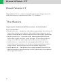
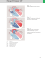
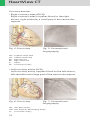
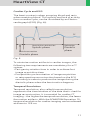
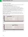
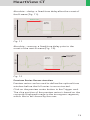
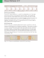
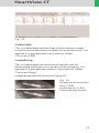
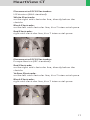
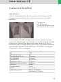
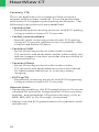
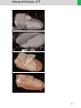
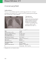
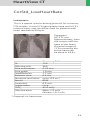
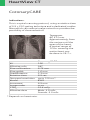
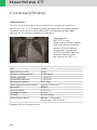
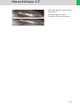
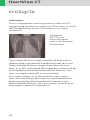
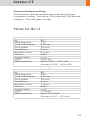
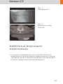
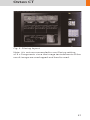
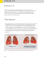
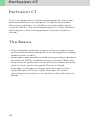
SOMATOM Sensation 10
Application Guide
Special Protocols
Software Version A60
The information presented in this application guide
is for illustration only and is not intended to be relied
upon by the reader for instruction as to the practice
of medicine. Any health care practitioner reading this
information is reminded that they must use their own
learning, training and expertise in dealing with their
individual patients.
This material does not substitute for that duty and is
not intended by Siemens Medical Solutions Inc., to be
used for any purpose in that regard. The drugs and
doses mentioned herein were specified to the best of
our knowledge. We assume no responsibility whatsover for the correctness of this information.
Variations may prove necessary for individual patients.
The treating physician bears the sole responsibility for
all of the parameters selected.
The pertaining operating instructions must always
be strictly followed when operating the SOMATOM
Sensation 10. The statutory source for the technical
data are the corresponding data sheets.
We express our sincere gratitude to the many customers
who contributed valuable input.
Special thanks to the former authors and editors
of this application guide, Bettina Klingemann
and Dr. Xiaoyan Chen for their great efforts and contribution.
To improve future versions of this application guide,
we would highly appreciate your questions, suggestions
and comments.
Please contact us:
CT Application Hotline:
Tel. no. +49-9191-18 80 88
Fax no. +49-9191-18 99 98
email: [email protected]
[email protected]
Editor: Ute Feuerlein
2
Overview
HeartViewCT
8
Bolus Tracking
38
Dental CT
46
Osteo CT
52
Pulmo CT
58
Perfusion CT
62
Dynamic Scanning
70
Interventional CT
72
Trauma
76
LungCARE
80
CT Colonography
82
Appendix
84
3
Content
HeartViewCT
· The Basics
– Important Anatomical Structures
of the Heart
– Cardiac Cycle and ECG
– Temporal Resolution
– Technical Principles
– Preview Series Reconstruction
– ECG Trace Editor
– ECG Pulsing
– CardioCARE
– CardioSharp
· How to do it
– CalciumScoring
· CaScoreSpiStd
· CaScoreSeqStd
· CoronaryStd
· CorStd_LowHeartRate
· CoronaryCARE
· CoronarySharp
· ECGtrigCTA
· LungECGHiRes
· PulmonaryECG
· Additional Important Information
4
8
8
8
11
11
12
13
14
14
15
15
16
16
18
19
22
23
24
26
28
31
32
33
Content
Bolus Tracking
· The Basics
· How to do it
· CARE Bolus
· TestBolus
· Additional Important Information
38
38
40
40
42
44
Dental CT
· The Basics
· How to do it
· Additional Important Information
46
46
47
49
OsteoCT
· The Basics
· How to do it
· Additional Important Information
52
52
53
55
Pulmo CT
· The Basics
· How to do it
· Additional Important Information
58
58
59
60
Perfusion CT
· The Basics
· How to do it
· Additional Important Information
62
62
64
67
Dynamic Scanning
· Scan Protocols
70
70
5
Content
6
Interventional CT
· The Basics
· How to do it
– Biopsy
– BiopsyCombine
· Additional Important Information
72
72
73
73
74
75
Trauma
· The Basics
· How to do it
– Trauma
– PolyTrauma
· Additional Important Information
76
76
77
77
78
79
LungCARE
· Scan Protocol
– Functionalities
80
80
81
CT Colonography
· Scan Protocol
82
82
Appendix
· Osteo CT
· Pulmo CT
84
84
86
Content
7
HeartView CT
HeartView CT
HeartView CT is a clinical application package specifically tailored to cardiovascular CT studies.
The Basics
Important Anatomical Structures of the Heart
Four chambers:
• Right atrium – receives the deoxygenated blood back
from the body circulation through the superior and
inferior vena cava, and pumps it into the right ventricle
• Right ventricle – receives the deoxygenated blood
from the right atrium, and pumps it into the pulmonary circulation through the pulmonary arteries
• Left atrium – receives the oxygenated blood back
from the pulmonary circulation through the pulmonary veins, and pumps it into the left ventricle
• Left ventricle – receives the oxygenated blood from
the left atrium, and pumps it into the body circulation
through the aorta
8
HeartView CT
Fig. 1:
Blood fills both atria
A
P
LV
RV
Fig. 2:
Atria contract, blood
enters ventricles
LA
RA
Fig. 3:
Ventricles contract,
blood enters into
aorta and pulmonary
arteries
A:
P:
RV:
LV:
RA:
LA:
Aorta
Pulmonary Artery
Right Ventricle
Left Ventricle
Right Atrium
Left Atrium
9
HeartView CT
Coronary arteries:
• Right coronary artery (RCA)
Right coronary artery supplies blood to the right
atrium, right ventricle, a small part of the ventricular
septum.
SVC A
PA
RA
RV
IVC
Fig. 4: Front view
SVC:
IVC:
RA:
RV:
A:
PA:
Fig. 5: Conventional
Angiography
Superior Vena Cava
Inferior Vena Cava
Right Atrium
Right Ventricle
Aorta
Pulmonary Artery
• Left coronary artery (LCA)
Left coronary artery supplies blood to the left atrium,
left ventricle and a large part of the ventricular septum.
LAD
➝
➝
LM
Cx ➝
Fig. 6: Front view
Fig. 7: Conventional
Angiography
LM: Left Main Artery
LAD: Left Anterior Descending Artery
Cx: Circumflex Artery
10
HeartView CT
Cardiac Cycle and ECG
The heart contracts when pumping blood and rests
when receiving blood. This activity and lack of activity
form a cardiac cycle, can be illustrated by an Electrocardiograph (ECG) (Fig. 8).
R
T
P
Q
U
S
Ventricular contraction
Relaxation
Systolic phase
Diastolic
phase
Atrial contraction
Diastolic phase
Fig. 8
To minimize motion artifacts in cardiac images, the
following two requirements are mandatory for a CT
system:
• Fast gantry rotation time in order to achieve fast
image acquisition time
• Prospective synchronization of image acquisition
or retrospective reconstruction based on the ECG
recording in order to produce the image during the
diastolic phase when the least motion happens.
Temporal Resolution
Temporal resolution, also called time resolution,
represents the time window of the data that is used for
image reconstruction. It is essential for cardiac CT
imaging – the higher the temporal resolution, the fewer
the motion artifacts. With the SOMATOM Sensation 10,
temporal resolution for cardiac imaging can be achieved
at down to 125 ms.
11
HeartView CT
Technical Principles
Basically, there are two different technical approaches
for cardiac CT acquisition:
• ECG triggered sequential scanning.
• Retrospectively ECG gated spiral scanning.
In both cases, an ECG is recorded and used to either
initiate prospective image acquisition (ECG triggering),
or to perform retrospective image reconstruction
(ECG gating). A given temporal relation relative to the
R-waves is predefined and can be applied with the
following possibilities:
Relative – delay: a given percentage of R-R interval
(%RR) relative to the onset of the previous or the next
R-wave (Fig. 9, 10).
50 % of R-R
ECG (t)
Scan/
Recon
Time
Fig. 9
ECG (t)
-50 % R-R
Scan/
Recon
Time
Fig. 10
12
HeartView CT
Absolute – delay: a fixed time delay after the onset of
the R-wave (Fig. 11).
400 msec
ECG (t)
Scan/
Recon
Time
Fig. 11
Absolute – reverse: a fixed time delay prior to the
onset of the next R-wave (Fig. 12).
Estimated
R-Peak
ECG (t)
Scan/
Recon
- 400 msec
Time
Fig. 12
Preview Series Reconstruction
Preview series can be used to define the optimal time
window before the full series is reconstructed.
Click on the preview series button in the Trigger card.
The slice position of the preview series is based on the
currently displayed image in the tomogram segment,
which has to be chosen by the user.
13
HeartView CT
ECG Trace Editor
The ECG trace editor is used for adaptation of image
reconstruction to irregular heart rates. This editing
tool can be used after the scan is acquired. By using
the right mouse menu on the Trigger card you can use
several modification tools for the ECG Sync, such as
Delete, Disable, Insert. To reset the ECG curve select
the check box Original ECG.
ECG Pulsing
ECG Pulsing is a dedicated technique used for online
dose modulation for Cardiac imaging. The tube current
is ECG-controlled and reduced during systolic phases
of the cardiac cycle while maintained normal during
diastolic phases when best image quality is required.
As shown in figure 13, essential dose reduction up to
50% can be achieved. It can be switched on/off by the
user (Fig. 14).
Fig. 13: Dose modulation with ECG pulsing.
14
HeartView CT
Fig. 14
CardioCARE
This is a dedicated cardiac filter which reduces image
noise thus provides the possibility of dose reduction. It is
applied in a pre-defined scan protocol called
“CoronaryCARE.”
CardioSharp
This is a dedicated reconstruction kernel used for
better edge definition in coronary artery imaging. It is
applied in a pre-defined cardiac scan protocol called
“CoronarySharp.”
Image examples are shown in figure 15.
15a
Fig. 15:
Image reconstruction
with (15b)
and without (15a)
Cardio Sharp kernel.
15b
15
HeartView CT
How to do it
Calcium Scoring
This application is used for identification and quantification of calcified lesions in the coronary arteries. It
can be performed with both ECG triggering (sequential scanning) and gating (spiral scanning) techniques.
The following scan protocols are predefined:
• CaScoreSpiStd
– Standard spiral scanning protocol with ECG gating
and a 0.5 s rotation time
• CaScoreSeqStd
– Sequential scanning protocol with ECG triggering
Hints in General:
• Kernel B35f is dedicated to calcium scoring studies.
To ensure the best image quality and correlation to
known reference data, other kernels are not recommended.
• Use the ECG triggered protocol generally except for
patients with arrhythmia. Use the ECG gated protocol
when accuracy and/or reproducibility are essential,
e. g. follow-up studies of calcium scoring or comparison studies with conventional angiography.
• The protocol with 0.5 s rotation time can be applied
to all examinations for HeartView CT.
Temporal resolution for cardiac imaging can be
achieved at down to 125 ms.
• We recommend a tube voltage of 120 kV. If the tube
voltage is lowered to 80 kV please use at least effective
mAs 250. The use of 80 kV is not advised for large
patients.
16
HeartView CT
Placement of ECG Electrodes:
US Version (AHA standard)
White Electrode
on the right mid-clavicular line, directly below the
clavicle
Black Electrode:
on the left mid-clavicular line, 6 or 7 intercostal space
Red Electrode:
right mid-clavicular line, 6 or 7 intercostal space
Placement of ECG Electrodes:
Europe Version (IEC standard)
Red Electrode
on the right mid-clavicular line, directly below the
clavicle
Yellow Electrode:
on the left mid-clavicular line, 6 or 7 intercostal space
Black Electrode:
right mid-clavicular line, 6 or 7 intercostal space
17
HeartView CT
CaScoreSpiStd
Indications:
This is a standard spiral scanning protocol, using
an ECG gating technique for coronary calcium scoring
studies, with a rotation time of 0.5 seconds.
Topogram:
AP, 512 mm.
From the carina until
the apex of the heart.
A typical range of
15 cm covering the
entire heart can
be done in 19.2 s.
kV
Effective mAs
Slice collimation
Slice width
Feed/Rotation
Rotation time
Temporal resolution
Kernel
Increment
Image order
CTDIw
Effective dose
* Depends on heart rate.
18
CaScoreSpiStd
120
133
1.5 mm
3.0 mm
4.5 mm
0.5 sec.
up to 125 ms*
B35f
1.5 mm
cr-ca
10.0 mGy
Male: 2.1 mSv
Female: 3.1 mSv
HeartView CT
CaScoreSeqStd
Indications:
This is a sequential scanning protocol using an ECG
triggering technique for coronary calcium scoring
studies.
Topogram:
AP, 512 mm.
From the carina until
the apex of the heart.
If you apply API for image acquisition, please make
sure that the breath-hold interval in the Patient Model
Dialog is longer than the total scan time, e. g. 50 s,
otherwise the image acquisition will be interrupted by
the default breath-hold interval. This does not apply
when API is not activated.
kV
Effective mAs
Slice collimation
Slice width
Feed/Scan
Rotation time
Temporal resolution
Kernel
Image order
CTDIw
Effective dose
CaScoreSeqStd
120
30
1.5 mm
3.0 mm
12.0 mm
0.5 sec.
250 ms
B35f
cr-ca
2.3 mGy
Male: 0.5 mSv
Female: 0.7 mSv
19
HeartView CT
Coronary CTA
This is an application for imaging of the coronary
arteries with contrast medium. It can be performed
with both ECG triggering and gating techniques. The
following scan protocols are predefined:
• CoronaryStd
– Standard spiral scanning protocol with ECG gating,
using a rotation time of 0.5 seconds.
• CorStd_LowHeartRate
– Special spiral scanning protocol with ECG gating,
using a 0.5 second rotation time, for patients with
a heart rate below 50 bpm.
• CoronaryCARE
– Spiral scanning protocol with rotation time
0.5 seconds and dedicated cardiac filter which can
reduce image noise thus provides the possibility of
dose reduction.
• CoronarySharp
– Spiral scanning protocol with rotation time
0.5 seconds and dedicated reconstruction kernel
for better edge definition in coronary artery
imaging.
• ECGTrigCTA
– Sequential scanning protocol with ECG triggering,
using a rotation time of 0.5 seconds.
General Hints:
• Generally speaking, the ECG gated protocol is recommended for premium image quality of the coronary
arteries, and whenever 3D postprocessing, such as
MPR, MIP, VRT or Fly Through, is required.
• Always use the ECG gated protocol for patients with
arrhythmia.
20
HeartView CT
21
HeartView CT
CoronaryStd
Indications:
This is a standard spiral scanning protocol, using a
rotation time of 0.5 s, with an ECG gating technique
for coronary CTA studies.
Topogram:
AP, 512 mm.
Approximately, from
the carina until the
apex of the heart.
A typical range of
12 cm covering the
entire heart can
be done in 28.7 s.
kV
Effective mAs
Slice collimation
Slice width
Feed/Rotation
Rotation time
Temporal resolution
Kernel
Increment
Image order
CTDIw
Effective dose
* Depends on heart rate.
22
CoronaryStd
120
500
0.75 mm
1.0 mm
2.3 mm
0.5 sec.
up to 125 ms*
B30f
0.5 mm
cr-ca
42.0 mGy
Male: 7.0 mSv
Female: 10.2 mSv
HeartView CT
CorStd_LowHeartRate
Indications:
This is a special spiral scanning protocol for coronary
CTA studies. It uses ECG gating technique and a 0.5 s
rotation time, and should be used for patients with
heart rate below 50 bpm.
Topogram:
AP, 512 mm.
Approximately, from
the carina until the
apex of the heart.
A typical range of
12 cm covering the
entire heart can
be done in 38.8 s.
kV
Effective mAs
Slice collimation
Slice width
Feed/Rotation
Rotation time
Temporal resolution
Kernel
Increment
Image order
CTDIw
Effective dose
CoronaryStdLow
120
500
0.75 mm
1.0 mm
1.7 mm
0.5 sec.
up to 125 ms*
B30f
0.5 mm
cr-ca
42.0 mGy
Male: 7.0 mSv
Female: 10.2 mSv
* Depends on heart rate.
23
HeartView CT
CoronaryCARE
Indications:
This is a spiral scanning protocol, using a rotation time
of 0.5 s, ECG gating technique and a dedicated cardiac
filter which can reduce image noise thus provides the
possibility of dose reduction.
Topogram:
AP, 512 mm.
Approximately, from
the carina until the
apex of the heart.
A typical range of
12 cm covering the
entire heart can
be done in 28.7 s.
kV
Effective mAs
Slice collimation
Slice width
Feed/Rotation
Rotation time
Temporal resolution
Kernel
Increment
Image order
CTDIw
Effective dose
* Depends on heart rate.
24
CoronaryCARE
120
267
0.75 mm
1.0 mm
2.3 mm
0.5 sec.
up to 125 ms*
B30f
0.5 mm
cr-ca
22.4 mGy
Male: 3.8 mSv
Female: 5.5 mSv
HeartView CT
25
HeartView CT
CoronarySharp
Indications:
This is a spiral scanning protocol, using a rotation
time of 0.5 s, ECG gating technique and a dedicated
cardiac reconstruction kernel for better edge definition in coronary artery imaging.
Topogram:
AP, 512 mm.
Approximately, from
the carina until the
apex of the heart.
A typical range of
12 cm covering the
entire heart can
be done in 28.7 s.
kV
Effective mAs
Slice collimation
Slice width
Feed/Rotation
Rotation time
Temporal resolution
Kernel
Increment
Image order
CTDIw
Effective dose
* Depends on heart rate.
26
CoronarySharp
120
500
0.75 mm
1.0 mm
2.3 mm
0.5 sec.
up to 125 ms*
B46f
0.5 mm
cr-ca
42.0 mGy
Male: 7.0 mSv
Female: 10.2 mSv
HeartView CT
a
Image reconstruction
with (b)
and without (a)
Cardio Sharp kernel.
b
27
HeartView CT
ECGTrigCTA
Indications:
This is a sequential scanning protocol with an ECG
triggering technique for coronary CTA studies. It could
also be applied for aortic CTA studies, e. g. aortic
dissection.
Topogram:
AP, 512 mm.
From the aortic
arch until the apex
of the heart.
If you apply API for a single breathhold acquisition,
please make sure that the breathhold interval in the
Patient Model Dialog is longer than the total scan
time, e. g. 50 s, otherwise the image acquisition will be
interrupted by the default breathhold interval. This
does not apply when API is not activated.
For longer ranges, e. g. the entire thoracic aorta,
that can not be acquired within a single breathhold,
please ensure that the breathhold interval in the
Patient Model Dialog is set up correctly, according to
the patient’s level of cooperation.
28
HeartView CT
kV
Effective mAs
Slice collimation
Slice width
Feed/Scan
Rotation time
Temporal resolution
Kernel
Image order
CTDIw
Effective dose
ECGTrigCTA
120
120
1.5 mm
1.5 mm
12.0 mm
0.5 sec.
250 ms
B30f
cr-ca
8.8 mGy
Male: 1.5 mSv
Female: 2.2 mSv
29
HeartView CT
Aortic and Pulmonary Studies
This application can be used for high-resolution interstitial lung studies with an ECG triggering technique,
or when imaging the aorta and pulmonary arteries
with contrast medium and ECG gating technique. The
following scan protocols are predefined:
• LungECGHires
– Sequential scanning protocol with ECG triggering
• PulmonaryECG
– Spiral scanning protocol with ECG gating
General Hints:
• The general purpose of these applications is to
reduce motion artifacts in the lungs due to the
cardiac pulsation.
• The LungECGHires protocol is recommended for
detection and localization of the lesions adjacent to
the heart or the interlobar fissures.
• The PulmonaryECG protocol is recommended for
aortic or pulmonary studies, e. g. aorta dissection or
pulmonary emboli.
30
HeartView CT
LungECGHires
Indications:
This is a sequential scanning protocol with an ECG
triggering technique for interstitial studies of the lungs,
especially for the lesions in the pericardial region.
Topogram:
AP, 512 mm.
From the apex of
the lung till the lung
base.
kV
Effective mAs
Slice collimation
Slice width
Feed/Scan
Rotation time
Temporal resolution
Kernel
Image order
CTDIw
Effective dose
LungECGHires
120
120
0.75 mm
0.75 mm
6.0 mm
0.75 sec.
375 ms
B80s
cr-ca
10.1 mGy
Male: 1.1 mSv
Female: 1.4 mSv
31
HeartView CT
PulmonaryECG
Indications:
This is a spiral scanning protocol with an ECG gating
technique for aortic and pulmonary studies, e. g. aortic
dissection or pulmonary emboli.
Topogram:
AP, 512 mm.
From the aorta arch
until the tip of the
sternum.
A typical range of
30 cm can be covered
in 28.9 s.
kV
Effective mAs
Slice collimation
Slice width
Feed/Rotation
Rotation time
Temporal resolution
Kernel
Increment
Image order
CTDIw
Effective dose
* Depends on heart rate.
32
PulmonaryECG
120
200
1.5 mm
3.0 mm
5.6 mm
0.5 sec.
up to 125 ms*
B30f
2.0 mm
cr-ca
15.0 mGy
Male: 5.7 mSv
Female: 7.3 mSv
HeartView CT
Additional Important
Information
By default, the “Synthetic Trigger” (ECG triggered
scanning) or “Synthetic Sync” (ECG gated scanning) is
activated for all predefined cardiac scan protocols
(Fig. 1 and 2). And it is recommended to keep it always
activated for examinations with contrast medium.
In case of ECG signal loss during the acquisition, this
will ensure the continuation of the triggered scans or
allows an ECG to be simulated for retrospective gating.
If it is deactivated, the scanning will be aborted in case
of ECG signal loss during the acquisition.
Fig. 1
Fig. 2
33
HeartView CT
ACV (Adaptive Cardio Volume) (Fig. 3) is a dedicated
algorithm for bi-phase image reconstruction. The image
temporal resolution of 125 ms can be achieved with
ACV. By default, it is switched on for all coronary CTA
scan protocols, and switched off for all calcium scoring
scan protocols. And it is not recommend to change this
default setting.
Fig. 3
34
HeartView CT
You can activate the “Auto load in 3D” function on the
Examination card/Auto Tasking and link it to a recon
job. If the postprocessing type is chosen from the pull
down menu, the reconstructed images will be loaded
automatically into the 3D card on the Navigator with
the corresponding postprocessing type.
On the 3D card you have the possibility to create for
MPR, MIPthin Range Parallel and Radial protocols which
can be linked to a special series.
For example, if you always do MIP Reconstructions for
a Coronary CTA examination, you load once the images
into the 3D card. Select the image type (e. g. MIPthin)
and the orientation, and then open the Range Parallel
function. Adapt the range settings (Image thickness,
Distance between the images etc.), hit the link and
save button. From now on, you have a predefined postprocessing protocol, linked to the series description of
a coronary CTA examination.
Exactly the same can be done for VRT presets. In the
main menu, under Type/VRT Definition, you can link
and save VRT presets with a series description.
Some of the Scan protocols are delivered with links
to a postprocessing protocol. If you do not like our
suggestions, please delete the Range Parallel preset or
overwrite them with your own settings.
35
HeartView CT
Calcium Scoring evaluation is performed on a separate
syngo task card:
1. The threshold of 130 HU is applied for score
calculation by default, however, you can modify it
accordingly.
2. In addition to the seeding method, you can use
freehand ROI for the definition of lesions.
3. The separation and modification of lesions within
a defined volume (depth in mm) can be performed
not only on 2D slices, but also with 3D editing.
4. For easier identification of small lesions, you can
blowup the display.
5. You can customize hospital/office information on
the final report using Report Configuration.
6. You can generate HTML report including site specific information, free text and clinical images. This
then can be saved on floppy disc and/or printed.
7. The results are displayed online in a separate
segment including the following information:
– Area (in mm3)
– Peak density (in HU)
– Volume (in mm3)
– Calcium mass (mg calcium Hydroxyapatite)
– Score (Agatston method)
8. The results can be printed on laser film, paper
printer or saved into data base.
36
HeartView CT
User interface of syngo Calcium Scoring
37
Bolus Tracking
The Basics
The administration of intravenous (IV) contrast
material during spiral scanning improves the detection
and characterization of lesions, as well as the opacity
of vessels. The contrast scan will yield good results
only if the acquisition occurs during the optimal phase
of enhancement in the region of interest. Therefore,
it is essential to initiate the acquisition with the correct
start delay. Since Multislice spiral CT can provide much
faster speed and shorter acquisition time, it is even
more critical to get the right timing to achieve optimal
results (Fig. 1a, 1b).
40 s scan
10 s scan
Fig. 1a: Longer scan time Fig. 1b: Shorter scan time
The dynamics of the contrast enhancement is
determined by:
• Patient cardiac output
• Injection rate (Fig. 2a, 2b)
• Total volume of contrast medium injected
(Fig. 3a, 3b)
• Concentration of the contrast medium (Fig. 3b, 4a)
• Type of injection – uni-phasic or bi-phasic (Fig. 4a, 4b)
• Patient pathology
38
Bolus Tracking
Aortic time-enhancement curves after i.v. contrast
injection (computer simulation*).
All curves are based on the same patient parameters
(male, 60-year-old, 75 kg).
* Radiology 1998; 207:647-655
Relative Enhancement [HU]
250
200
150
100
50
0
0
Relative Enhancement [HU]
300
300
250
200
150
100
50
20
40
60
80
100
120
0
0
20
40
Fig. 2a: 2 ml/s,
120 ml, 300 mg I/ml
80
100
120
100
120
Fig. 2b: 4 ml/s,
120 ml, 300 mg I/ml
Relative Enhancement [HU]
250
200
150
100
50
0
Relative Enhancement [HU]
300
300
0
60
Time [s]
Time [s]
250
200
150
100
50
20
40
60
80
100
120
0
0
20
40
60
80
Time [s]
Time [s]
Fig. 3a: 80 ml,
4 ml/s, 300 mg I/ml
Fig. 3b:120 ml,
4 ml/s, 300 mg I/ml
Relative Enhancement [HU]
350
300
250
200
150
100
250
200
150
100
50
50
0
0
Relative Enhancement [HU]
300
400
20
40
60
80
Time [s]
Fig. 4a: Uni-phase
140 ml, 4 ml/s,
370 mg I/ml
100
120
0
0
20
40
60
80
100
120
Time [s]
Fig. 4b: Bi-phase
70 ml, 4 ml/s, plus 70 ml,
2 ml/s, 370 mg I/ml
39
Bolus Tracking
How to do it
To achieve optimal results in contrast studies, the use
of CARE Bolus is recommended. In case it is not available,
use Test Bolus.
CARE Bolus
This is an automatic bolus tracking program, which
enables triggering of the spiral scanning at the optimal
phase of the contrast enhancement.
General Hints:
1. This mode can be applied in combination with
any spiral scanning protocol. Simply insert “Bolus
tracking” by clicking the right mouse button in
the chronicle. This inserts the entire set up including
pre-monitoring, i.v. bolus and monitoring scan
protocol. You can also save the entire set up as your
own scan protocols (please refer to the application
guide for routine protocols).
2. The pre-monitoring scan is used to determine the
level of monitoring scans. It can be performed at
any level of interest. You can also increase the mAs
setting to reduce the image noise when necessary.
3. To achieve the shortest possible spiral start delay
(2 s), the position of the monitoring scans relative
to the beginning of spiral scan must be optimized.
A “snapping” function is provided:
40
Bolus Tracking
– After the Topogram is performed, the predefined
spiral scanning range and the optimal monitoring
position will be shown.
– If you need to redefine the spiral scanning range,
you should also reposition the monitoring scan in
order to keep the shortest start delay time (2 s).
(The distance between the beginning of the spiral
scanning range and the monitoring scan will be
the same).
– Move the monitoring scan line towards the optimal position and release the mouse button, it will
be snapped automatically. (Trick: if you move the
monitoring scan line away from the optimal position the “snapping” mechanism will be inactive).
4. Place an ROI in the premonitoring scan on the
target area or vessel used for triggering. (The ROI
is defined with double circles – the outer circle is
used for easy positioning, and the inner circle is
used for the actual evaluation). You can also zoom
the reference image for easier positioning of the
ROI.
5. Set the appropriate trigger threshold, and initiate
the contrast injection and monitoring scans at the
same time.
During the monitoring scans, there will be simultaneous display of the relative enhancement of the
target ROI. When the predefined density is reached,
the spiral acquisition will be triggered automatically.
6. You can also initiate the spiral any time during the
monitoring phase manually – either by pressing the
START button or by clicking the START key. If you
do not want to use automatic triggering, you can
deselect it.
41
Bolus Tracking
TestBolus
Indications:
This mode can be used to test the start delay of an
optimal enhancement after the contrast medium
injection.
kV
Effective mAs
Slice collimation
Slice width
Feed/Scan
Rotation time
Kernel
Cycle time
42
TestBolus
120
30
5.0 mm
10.0 mm
0 mm
0.5 sec.
B40f
2 sec.
Bolus Tracking
Application procedures:
1. Select the spiral mode that you want to perform,
and then “Append” the TestBolus mode under Special
protocols.
2. Insert the Test Bolus mode above the spiral mode
for contrast scan by “cut/paste” (with right mouse
button).
3. Perform the Topogram, and define the slice position
for TestBolus.
4. Check the start delay, number of scans and cycle
time before loading the mode.
5. A test bolus with 10-20 ml is then administered
with the same flow rate as during the following spiral
scan. Start the contrast media injection and the
scan at the same time.
6. Load the images into the Dynamic Evaluation
function and determine the time to the peak enhancement.
Alternatively, on the image segment, click “select series”
with the right mouse button and position an ROI on
the first image. This ROI will appear on all images in
the test bolus series. Find the image with the peak HU
value, and calculate the time “delta t” taken to reach
the peak HU value (do not forget to add the preset
start delay time). This time can then be used as the
optimal start delay time for the spiral scan.
43
Bolus Tracking
Additional Important
Information
1.The preset start delay time for monitoring scans
depends on whether the subsequent spiral scan will
be acquired during the arterial phase or venous
phase. The default value is 10 s. You can modify it
accordingly.
2. It should be pointed out that when using “Test
Bolus”, there may be residual contrast in the liver
and kidneys prior to scanning. This may result in
an inaccurate arterial and equilibrium phase.
3. The trigger threshold is not an absolute value but
a relative value compared to the non-contrast scan.
E. g. if the CT value is 50 HU in the non-contrast
image, and your trigger level is 100 MU, then the
absolute CT value in the contrast image will be
150 HU.
4. If you change slice collimation, rotation time or kV
in the spiral scanning protocol after CARE Bolus
is inserted, a longer spiral start delay time will be
the result, e. g. 14 s. This is due to the necessary
mechanical adjustments, e. g. moving the slice
collimators. Therefore, it is recommended that you
modify the parameters of the spiral scanning
before inserting the CARE Bolus.
44
Bolus Tracking
5. If API is used in conjunction with CARE Bolus, the
actual start delay time for the spiral will be as long
as the length of API including the predefined start
delay time. E. g. if the predefined the start delay is
2 s, and the API lasts 5 s, the spiral will start 5 s after
the threshold is reached.
6. In case you have to interrupt the monitoring
scanning due to injection problem, you can repeat it
afterwards by inserting CARE Bolus again with a
right mouse click. The same Topogram can still be
used.
45
Dental CT
Dental CT
This is an application package for reformatting panoramic views and paraxial slices through the upper and
lower jaw. It enables the display and measurement
of the bone structures of the upper and lower jaw
(especially for a 1:1 scale) as the basis for OR planning
in oral surgery.
The Basics
What is the relevant anatomical information for oral
surgery planning and dental implantation?
• Location of the socket for dental implant,
• Buccal and lingual thickness of the cortical component of the alveolar process,
• Position of the mandibular canal and the mental
foramen,
• Extent of the nasal sinuses and
• Position and width of the floor of the nasal cavity.
What can Dental CT do?
• Reformatting of a curvilinear range of panoramic
views along the jaw-bone.
• Reformatting of paraxial views of selectable length
and at selectable intervals perpendicular to the
panoramic views.
• Presentation of results in the form of multiple image
display with reference markings.
• Images are documented on film in “real-size” so that
the direct measurement of the anatomic information
with a ruler is possible. The layout of the film sheet is
predefined such that it can accommodate the maximum number of reformatted images.
46
Dental CT
Fig. 1:
Panoramic view
Fig. 2:
Paraxial view
How to do it
Scan Protocol:
kV
Effective mAs
Slice collimation
Slice width
Feed/Rotation
Rotation time
Kernel
Increment
Image order
CTDIw
Effective dose
Dental
120
80
0.75 mm
0.75 mm
5.0 mm
0.75 sec.
H60s
0.5 mm
cr-ca
17.1 mGy
Male: 0.3 mSv
Female: 0.3 mSv
47
Dental CT
• It is mandatory to position the patient head in the
center of the scan field – use the lateral laser light
marker for positioning.
• Gantry tilt is not necessary since you have the possibility to tilt the reference line to generate an axial
reformatted image at the desired plane. However,
in order to minimize the scan length for the same
anatomical region, it is recommended to position the
patient’s head at the appropriate scan plane whenever possible:
– For the upper and lower jaw:
occlusal plane in parallel to the scan plane.
– For either jaw:
jaw bone in parallel to the scan plane.
• It is recommended to end the exam first, and then
start the Dental evaluation.
Fig. 3: User interface of syngo Dental
48
Dental CT
Additional Important
Information
• This protocol delivers high resolution images for
Dental CT evaluation, however, you can also reconstruct images with softer kernel, e. g. H20s, for
3D/SSD postprocessing.
Fig. 4a:
AP-cranial view
Fig. 4b:
Caudal view
• Image orientation:
– In the paraxial view, a “B” indicates buccal and
a “L” lingual. The lingual marker “+” must always be
positioned at the tongue. If not, simply drag & drop
it back.
– In the panoramic view, a “B” stands for “Begin” and
an “E” for “End”.
• Filming: for the maximum use of the film, film directly
from the Dental Card instead of Patient Browser.
For easy reprinting, the results of the latest Dental CT
Film are stored in the Patient Browser in the folder
“Film”.
• It is better to change the image windowing on the
virtual film sheet.
• A semi-automatic detection tool can be used to mark
and outline the mandibular canal on both paraxial
and panoramic images for easy viewing and filming.
49
Dental CT
• Multiple paraxial ranges can be defined on one
reference image by “cluster & copy function”. I. e.,
you can group a number of paraxial lines and copy
the lines to another location, e. g. over individual
sockets at different locations (Fig.5).
• ROI definition for statistical evaluations and deletion
of graphics are possible.
Fig. 5
50
Dental CT
51
Osteo CT
Osteo CT
This is an application package for the quantitative
assessment of vertebral bone mineral density for
the diagnosis and follow-up of osteopenia and osteoporosis.
The Basics
This program enables the quantitative determination
of bone mineral density of the spine in mg/ml of calcium
hydroxyapatite (CaHA) for the diagnosis, staging, and
follow-up of osteopenia and osteoporosis with CT. The
patient is scanned together with the water- and boneequivalent calibration phantom.
What is “T-score”?
This is the deviation of average BMD of the patient
from that of a young healthy control. It represents
bone loss with reference to the peak bone mass.
What is “Z-score”?
This is the deviation of average BMD of the patient
from that of a healthy person of the same age. It is an
indicator of biological variability.
52
Osteo CT
Siemens Reference Data:
The Siemens reference data was acquired at three
European centers, including 135 male and 139 female
subjects, 20 to 80 years of age.
How to do it
kV
Effective mAs
Slice collimation
Slice width
Feed/Scan
Rotation time
Kernel
Image order
CTDIw
Effective dose
Osteo
80
125
5.0 mm
10 mm
0 mm
0.5 sec.
S80f
cr-ca
2.6 mGy
Male: 0.02 – 0.03 mSv
Female: 0.03 – 0.03 mSv
kV
Effective mAs
Slice collimation
Slice width
Feed/Scan
Rotation time
Kernel
Image order
CTDIw
Effective dose
OsteoObese
80
350
5.0 mm
10 mm
0 mm
1.5 sec.
S80s
cr-ca
7.0 mGy
Male: 0.07 mSv
Female: 0.07 – 0.2 mSv
53
Osteo CT
Patient positioning:
• Set the table height at 125. The gantry tilt will be
available from –22° to +22°.
• Patients should be positioned so they are as parallel
to the patient table as possible. Support the knees to
compensate for lordosis.
• The calibration phantom should be positioned
directly below the target region. Put the Gel-pad between the calibration phantom and the patient to
exclude air pockets.
Scanning:
• Typically, one scan each is performed at L1, L2 and
L3 levels. It is recommended to use image comments
L1, L2, L3 prior to scanning. These comments will be
displayed with the Osteo evaluation results.
• Before ending the examination, you can drag & drop
the chronicles to the topogram segment to get the
Topographics, i. e. the cut lines for each vertebra on
the topogram.
• Select the appropriate scan protocol according to the
patient size, i. e. use “OsteoObese” for obese patient.
• Position the cut line of scanning through the middle
of the vertebra, i. e. bi-sector between the angle of the
upper and lower end plate.
• The phantom must be included in the FoV of the
images for evaluation.
• It is recommended to end the exam first, and then
start the Osteo evaluation.
54
Osteo CT
Fig. 1:
Topographic
Fig. 2:
Phantom inside
the FoV
Additional Important
Information
• Fractured vertebrae are not suited for Osteo CT
evaluation since the more compact nature of these
vertebrae result in bone mineral density value that
is much higher than one would expect.
55
Osteo CT
• How to save the results on your PC?
– Select Option/Configuration from the main menu
and click icon ”CT Osteo”.
– Activate the checkbox “Enable Export of Results”.
– “Exit” the configuration dialog.
– Call up the Osteo card and you will see the new
icon “Export results” on the lower, right part of the
screen.
– Click this icon to copy the evaluation results to
floppy disk (Note: with every mouse click on the
icon, the previous result file will be appended).
– The data file can be transferred to your PC for
further evaluation, e. g. with MS Excel.
Note: for detailed information about the data file,
please refer to the Appendix.
• It is recommended to film directly from the Osteo
card. Select images or series with Edit/Select all,
and click “film” icon. You can also configure film
layout, e. g. 3 x 3 as shown in figure 3 in Option/
Configuration/FilmingLayout.
56
Osteo CT
Fig. 3: Filming layout
Note: it is not recommended to use filming setting
of 4 x 5 segments since the image text elements of the
result image are overlapped and hard to read.
57
Pulmo CT
Pulmo CT
This is an application package, which serves for
quantitative evaluation of the lung density to aid the
diagnosis and follow-up of diffuse lung diseases,
such as pulmonary emphysema, sarcoidosis, panbronchiolitis and silicosis.
The Basics
• No specific scan protocols were set up for this option.
Scan protocols for routine thorax imaging can be
used. The scan parameters used are dependent on
the indications and objectives of the study design.
For example, spiral mode for lung volume evaluation
or HR sequence mode for interstitial lung diseases.
• Lung density is influenced by respiratory status
(Fig.1).
Full Inspiration
Full Expiration
Density = @
Density = >2 x @
Fig. 1: Lung density at full inspiration/expiration
58
Pulmo CT
• Examinations should be acquired at the same respiratory level, usually at either full inspiration or full
expiration. Studies had shown that reproducibility
is high and is unlikely to be improved by using spirometric gating [1].
Literature
1. Repeatability of Quantitative CT Indexes of
Emphysema in Patients
Evaluated for Lung Volume Reduction Surgery.
David s. Gierada et al, Radiology 2001 220: 448-454
Siemens Reference Data
It was acquired from lung healthy individuals at 50%
vital capacity. Since Pulmo CT program does not provide spirometric triggering for the acquisition of the
data set, it is not meaningful to use Siemens reference
data for comparison unless the data is acquired under
the same conditions.
User-Specific Reference Data
It is possible to integrate in your own reference data,
e. g. data acquired at full inspiration, for the evaluation.
Please contact the local Siemens representative for
further information.
How to do it
It is recommended to end the exam first, and then
start the Pulmo evaluation.
Select the images that you want to evaluate, and
activate the program by clicking on the “Pulmo” icon.
59
Pulmo CT
Additional Important
Information
• How to export the evaluation results to a floppy disc?
– Select Option/Configuration from the main menu
and click icon “Pulmo”.
– Activate the checkbox “Enable Export of Results”.
– “Exit” the configuration dialog.
– Call up the Pulmo card and you will see the new
icon “Export results” on the lower, right part of the
screen.
– Click this icon to copy the evaluation results onto
floppy disk. (Note: with every mouse click on the
icon, the previous result file on the floppy will be
appended).
– The data file can be transferred to your PC for
further evaluation, e. g. with MS Excel.
Note: for detail information about the data file,
please refer to the Appendix.
• Standard and expert mode can be configured to your
needs.
– Select Option/Configuration/Pulmo.
For example, if you want to determine the percentage area of the lung within a specific HU range,
use the card “Subranges” on the Configuration/
Pulmo dialog.
• Color-coded display of HU subranges and percentiles
is possible. This allows direct visualization of the
different densities distribution within the lung.
• The auto-contour detection can be used as editing
function for 3D postprocessing of lung images.
60
Pulmo CT
Fig. 2: User interface of syngo Pulmo
61
Perfusion CT
Perfusion CT
This is an application software package for the quantitative evaluation of dynamic CT data of the brain
following injection of a highly concentrated iodine
contrast bolus. The main application is in the differential diagnosis and management of acute ischemic
stroke.
The Basics
• The software optimally supports the stringent time
and workflow requirements in an emergency setting
where time is brain.
• Parameters generated include among others cerebral
blood flow (CBF), cerebral blood volume (CBV), the
time to local perfusion onset (Time-to-Start) and the
time to local perfusion peak (Time-to-Peak).
• Example: A 44-year-old man was brought to the
hospital about 2 hours after the start of severe
neurological symptoms of stroke in the right hemisphere.
62
Perfusion CT
Fig. 1: User interface of syngo Perfusion
The CBF image shows a severe perfusion disturbance
(flow close to zero) in the insular cortex and the posterior portion of the lentiform nucleus. In comparison to
the left hemisphere the remaining supply area of the
middle cerebral artery shows moderately reduced flow.
• The CBV image shows the same severe reduction in
insular cortex and lentiform nucleus. In contrast to
the CBF image, however, the blood volume in the
remaining right MCA territory is close to normal, if it
is compared to the same area on the left side.
• The time-to-peak image shows a general prolongation of values in the MCA territory indicating delayed
bolus arrival.
63
Perfusion CT
How to do it
Scan protocols
There are two Scan protocols available:
BrainPerfCT, a non contrast study and a Dynamic
Serio with 12 mm collimation and 2 times a 12 mm
slice thickness.
BrainPerfSingle, a non contrast study and a Dynamic
Serio with 5.0 mm collimation and one 10 mm slice
thickness.
BrainPerfCT
kV
Effective mAs
Slice collimation
Slice width
Feed/Scan
Rotation time
Cycle time
Kernel
Image order
NonContrast
120
320
3.0 mm
9.0 mm
18 mm
1.0 sec.
3.0 sec.
H30s
ca-cr
DynSerio
80
140
12.0 mm
12.0 mm
0 mm
0.5 sec.
0.75 sec.
H30f
ca-cr
BrainPerfSingle
kV
Effective mAs
Slice collimation
Slice width
Feed/Scan
Rotation time
Cycle time
Kernel
Image order
NonContrast
120
320
3.0 mm
9.0 mm
18 mm
1.0 sec.
3.0 sec.
H30s
ca-cr
DynSerio
80
168
5.0 mm
10.0 mm
0 mm
0.5 sec.
0.75 sec.
H30f
ca-cr
Such a standard protocol may be slightly modified for
specific reasons; e. g. the start delay can be increased
by a few seconds for patients with very low cardiac
output.
64
Perfusion CT
IV injection protocol
Contrast medium
Non-ionic
Concentration
300 – 370 ml
Injection rate
8 ml/sec.
Total volume
40 ml
Total injection time ~ 5 sec.
Start delay time
4 sec
The technique requires a short bolus. The original
studies were performed mostly using 50 ml injected at
10 ml/s.
The routine application has shown, that by sacrificing
some of the spatial resolution, the examination can also
be done with smaller amounts of contrast (35 to 40 ml)
and correspondingly smaller flow rates. The smaller the
total amount the more helpful it is to consider a saline
chaser bolus. In any case, a state-of-the-art power
injector is recommended.
If a flow rate of 8 ml/s is considered not recommendable for a specific patient, the protocol can be reduced
to 40 ml at 5ml/s. Image quality will be reduced but
the technique will still be diagnostic.
• Additional measures to facilitate the injection, like
using a large gauge cannula (16 or 18 are usually
sufficient) and warming the contrast media to body
temperature to reduce its viscosity, should be considered.
Note: As with any contrast medium application,
verify that the particular models and brands that you
use in the chain injector/contrast medium/cannula
are approved by their respective manufactures for
the use with the parameters you select.
• Motion during acquisition must be avoided. Therefore, if at all possible you should try to explain the
course of the examination to the patient and use
additional head fixation in any case.
65
Perfusion CT
• The standard examination slice is best positioned
such that it cuts through the basal ganglia at the level
of the inner capsule. This selection includes those
vascular territories of the brain that are frequently
affected by perfusion impairment associated with
acute stroke in the carotid territory.
• The slice should be selected “flatter“ than in normal
head CT scan, the angulation should be adjusted perpendicular to the occipital segment of the superior
sagittal sinus well above the confluence of sinuses.
• The eye lens should never be positioned in the scan
plane.
Example of a
standard slice
through the basal
ganglia in a
lateral topogram.
66
Perfusion CT
Additional Important
Information
1. Why short injection times are necessary?
The brain has a very short transit time (approx. 3 to
5 seconds) and a relatively small fractional blood volume
(approx. 2 to 5%). This requires a compact bolus for
optimal time resolution and a certain minimum amount
of contrast for optimal signal to noise ratio. Bolus definition can be significantly improved and the amount
of contrast necessary reduced by using a saline chaser
bolus with the same flow rate directly following the
CM injection.
2. What do normal, contrast-enhanced and Perfusion
CT images show?
In order to interpret Perfusion CT images correctly,
it is essential to understand that they are “functional“
or “parameter“ images that display a different type
of information than standard CT images: Normal CT
images basically show only morphological properties
of tissues by displaying their x-ray attenuation relative
to that of water as CT-values in HU-units.
Standard contrast-enhanced CT extends this limitation
either to make a compartment visible that normally
has low contrast (e. g. vascular structures in CTA) or
to qualitatively display major perfusion differences of
tissues (e. g. tumors or multiphase liver studies).
Perfusion CT tries to utilize all the information hidden
in the temporal changes of contrast enhancement by
fitting a mathematical model to the local time attenuation curves. For each voxel this process yields a variety
of numbers which describe different aspects of tissue
perfusion. As the human eye is so much faster and
better suited to interpret images than large amounts
of numbers it makes sense to display these quantities
in the form of images.
67
Perfusion CT
3. What do pixel values mean in the Perfusion CT
images?
It is very important to realize that pixel values now
have a different meaning, which depends on the type
of image currently displayed. So if you point the cursor
into a parameter image bear in mind that you do not
read a CT-value but a functional unit. A time-to-peak
image, for example, displays numbers proportional to
the time until the bolus peak is reached; so higher
numbers mean later bolus arrival.
A CBF image, on the other hand, displays numbers
proportional to blood flow; so smaller numbers indicate
lower flow.
4. Filming color images
If a color hardcopy device is connected to the system,
color images can be printed via the filming task card.
It is recommended to send the color images from the
Viewing task card after having saved them on the Perfusion task card.
5. How to fine-tune the color mapping?
– For “flow images” (CBF and CBV) – the color palette
for the flow image is designed such, that after optimal
adjustment with the arrow buttons the following
approximate correspondence will result for a normal
brain:
red _ vessels
green/yellow _ gray matter
blue _ white matter
black _ no calculation (CSF space)
68
Perfusion CT
After adjustment (use non-ischemic hemisphere as
guideline) ischemic areas will therefore be displayed
either in violet (very low flow) or as a mismatch with
the nonischemic side (gray matter is blue instead of
green).
– For “Time images” (Time to Start and Time to Peak) –
the color palette for the time images maps increasing time values on a spectral scale:
Violet _ blue _ green _ yellow _ red
Display should be adjusted with the arrow buttons
such that the areas with latest arrival times are just
slightly red. As with the flow image black means no
calculation (CSF space, or areas with extremely low
flow – no time assessment possible).
69
Dynamic Scanning
Dynamic Scanning
These are protocols templates for the analysis of
contrast enhancement dynamics in the body. Scan
parameter details such as mAs, slice width, increment etc. depend on the organ to be studied.
These may be used with the Dynamic Evaluation
function for the descriptive analysis of contrast enhancement of tissues.
Scan Protocols
There are two scan protocols available:
BodyDynCT, a Serio Mode with a 12 mm slice
collimation and 2 times a 12 mm slice width.
BodyDynSingle, a Serio Mode with a 5 mm slice
collimation and one 10 mm slice width.
70
Dynamic Scanning
kV
Effective mAs
Slice collimation
Slice width
Feed/Scan
Rotation time
Cycle time
Kernel
BodyDynCT
120
100
12.0 mm
12.0 mm
0 mm
0.5 sec.
1.0/5.0 sec.
B30f
kV
Effective mAs
Slice collimation
Slice width
Feed/Scan
Rotation time
Cycle time
Kernel
BodyDynSingle
120
100
5.0 mm
10.0 mm
0 mm
0.5 sec.
1.0/5.0 sec.
B30f
71
Interventional CT
Interventional CT
To facilitate CT interventional procedures, we created
dedicated multislice and single slice sequential modes.
• Biopsy
This is the multislice biopsy mode. E. g. 6 slices,
3.0 mm each, will be reconstructed and displayed for
each scan.
• BiopsyCombine
This is a single slice biopsy mode. 2 x 5 mm slice
collimation is used to get a combined 10 mm slice.
The Basics
Any of these protocols can be appended to a spiral
protocol for CT interventional procedures, such
as biopsy, abscess drainage, pain therapy, minimum
invasive operations, joint studies, and arthrograms.
10 scans are predefined. You can repeat it by clicking
the chronicle with the right mouse button and select
“repeat”, or simply change the number of scans to 99
before you start the first scan.
You can “Append” any routine protocol after the
interventional procedure for a final check and documentation, e. g. a short range of spiral scanning for
the biopsy region.
The table height can be adjusted to minimum
255 mm.
72
Interventional CT
How to do it
Biopsy
Indications: This is the multislice biopsy mode. 6 slices,
3.0 mm each, will be reconstructed and displayed for
each scan. It can be appended to any other scan protocol, e. g. ThoraxRoutine for biopsy procedures in the
thorax. Change the mAs setting accordingly before you
load the mode.
kV
Effective mAs
Slice collimation
Slice width
Feed/Scan
Rotation time
Kernel
Biopsy
120
120
3.0 mm
3.0 mm
0 mm
0.5 sec.
B30f
Application procedures:
1. Perform a spiral scan first to define a target slice.
2. Click “Same TP” under Table position in the routine
card, and move the table.
3. Turn on the light marker to localize the Entry point,
and then start the patient preparation.
4. Select “Biopsy” mode under Special protocols, and
then click “Append”.
73
Interventional CT
5. Click “Load” and then “Cancel move”. Press the
“Start” button and 6 images will be displayed.
6. Press “Start” again, you’ll get another 6 images with
the same slice position.
BiopsyCombine
Indications: This is the biopsy mode with one combined slices. It can be appended to any other scan
protocol, e. g. ThoraxRoutine for biopsy procedures
in the thorax.
Change the mAs setting accordingly before you load
the mode.
kV
Effective mAs
Slice collimation
Slice width
Feed/Scan
Rotation time
Kernel
BiopsyCombine
120
120
5.0 mm
10 mm
0 mm
0.5 sec.
B30f
Application procedures:
1. Perform a spiral scan first to define a target slice.
2. Click “Same TP” under Table position in the routine
card, and move the table.
3. Turn on the light marker to localize the Entry point,
and then start the patient preparation.
4. Select “BiopsyCombine” mode under Special protocols, and then click ”Append”.
5. Click “Load” and then “Cancel move”. Press the
“Start” button and one image will be displayed.
6. Press “Repeat” and “Start” again, you’ll get another
image with the same slice position.
74
Interventional CT
Additional Important
Information
• In the BiopsyCombine mode, the slice position, table
position, table begin and table end are all the same.
• In the Biopsy mode, the slice position, table position,
table begin and table end are different.
a) The SP (slice position) in each image means the
center of the image (Fig. 1).
Image 1
Image 2
Image 3
Image 4
Image 5
Image 6
SP
SP
SP
SP
SP
SP
Fig. 1
b) The “Table position” means the central position
of the 6 images and will also be the position of the
positioning light marker (Fig. 2).
Image 1
Image 2
Image 3
Image 4
Image 5
Image 6
Table “position”
Fig. 2
c) The table “Begin” means the center of the first
image, and the table “End” means the center of the
last image (Fig. 3).
Image 1
Image 2
Table “Begin”
Image 3
Image 4
Image 5
Image 6
Table “End”
Fig. 3
75
Trauma
Trauma
In any trauma situation, time means life and the
quality of life for the survivor. In order to facilitate the
examinations, two protocols are provided:
• Trauma
This is a one-range mode for fast screening
• PolyTrauma
This is a combined mode for the examination of
multiple ranges, e. g. Head, Neck, Thorax, Abdomen
and Pelvis
The Basics
• Check that the emergency drug trolley is well-stocked
and that all accessories such as in-room oxygen
supply, respirator and resuscitation equipment that
may be required during the examination are in working order.
• Prepare the CT room before admitting the patient,
e. g., load IV contrast into the injector.
• Know, observe and practice the standard hospital
operating policy for handling a patient in distress
e. g. Code Blue for cardiac and respiratory arrest.
• Any possible injuries to the spinal column should be
determined before beginning the examination and
taken into account when shifting and positioning the
patient.
• Ensure that all vital lines e. g., IV tubing and oxygen
tubing are not trapped under the patient or between
the table and the cradle. Make allowance for the
length of tubing required for the topogram scan range.
76
Trauma
• Never leave patients unattended at any time during
the procedure.
• Observe the vital signs e. g. ECG, respiration, etc. at
all times during the procedure.
• Finish the examination in the shortest possible time.
How to do it
Trauma
Scan Protocol:
kV
Effective mAs
Slice collimation
Slice width
Feed/Rotation
Rotation time
Kernel
Increment
Image order
CTDIw
Effective dose
Trauma
120
140
1.5 mm
7.0 mm
15.0 mm
0.5 sec.
B31f
7.0 mm
cr-ca
10.5 mGy
Male: 7.2 mSv
Female: 8.9 mSv
You can adjust the mAs setting according to the region
to be examined.
77
Trauma
PolyTrauma
Scan Protocol:
PolyTrauma
kV
Effective mAs
Slice collimation
Slice width
Feed/Rotation
Rotation time
Kernel
Increment
Image order
CTDIw
Effective dose
HeadFastSpi
120
260
1.5 mm
6.0 mm
10.5 mm
0.75 sec.
H31s
6.0 mm
ca-cr
49.1 mGy
Male: 2.0 mSv
Female: 2.1 mSv
NeckFastspi
120
150
1.5 mm
5.0 mm
12.0 mm
0.5 sec.
B31f
5.0 mm
cr-ca
11.3 mGy
Male: 1.5 mSv
Female: 1.6 mSv
PolyTrauma
kV
Effective mAs
Slice collimation
Slice width
Feed/Rotation
Rotation time
Kernel
Increment
Image order
CTDIw
Effective dose
ThoraxFast
120
110
3.0 mm
7.0 mm
18.0 mm
0.5 sec.
B41f
7.0 mm
cr-ca
7.7 mGy
Male: 2.6 mSv
Female: 3.4 mSv
AbdPelRoutine
120
140
3.0 mm
7.0 mm
18.0 mm
0.5 sec.
B31f
7.0 mm
cr-ca
9.8 mGy
Male: 5.9 mSv
Female: 8.5 mSv
In different polytrauma cases, you could either combine different protocols, or delete any of the chronicles
from the predefined protocol if they are not needed.
78
Trauma
Additional Important
Information
• For long range scanning, please pay attention to the
mark of scannable range on the table mattress while
positioning the patient.
• In some cases, it might be advisable to position the
patient as Feet first so that there will be more space
for the intensive care equipment around.
• The Trauma protocol is predefined with a Topo
length of 1024 mm, the Poly Trauma protocol with a
Topo length of 1536 mm.
Note: You should press the “Hold Measurement“
button whenever the range shown on the real time
growing topogram is long enough, in order to avoid
unnecessary radiation.
79
LungCARE
A dedicated low dose Spiral mode for the syngo
LungCARE evaluation.
Indications:
Lung studies with low dose setting, e. g. early visualization of pulmonary nodules.
A typical thorax study in a range of 30 cm will be
covered in 14.3 s.
kV
Effective mAs
Slice collimation
Slice width
Feed/Rotation
Rotation time
Kernel
Increment
Image order
CTDIw
Effective dose
LungCARE
120
20
0.75 mm
1.0 mm
11.3 mm
0.5 sec.
B50f
0.5 mm
cr-ca
1.6 mGy
Male: 0.6 mSv
Female: 0.8 mSv
We recommend using a tube voltage of at least
120 kV.
For further information on the syngo LungCARE
Application, please refer to the Application Guide
“Clinical Options”.
80
LungCARE
Fig. 1: User interface of syngo LungCARE
syngo LungCARE is a dedicated software for visualization and evaluation of pulmonary nodules using lowdose lung scanning and for subsequent follow-up
studies.
Functionalities
• 3D Visualization with Thin Slabs using MPR, MIP
and VRT displays.
• Computer-guided localization of pre-marked lesion.
• Close-up inspection of suspected lesion with the
Rotating MPR mode.
• Automatic evaluation of pulmonary nodules with
perspective VRT or MPR display.
• Automatic volume and diameter measurements of
pulmonary nodules.
• Easy and flexible reporting of the evaluated nodules.
81
CT Colonography
For Colonography studies.
A typically range of 40 cm can be covered in 22.4 s.
CT Colonography
kV
120
Effective mAs
100
Slice collimation 0.75 mm
Slice width
5.0 mm
Feed/Rotation
9.4 mm
Rotation time
0.5 sec.
Kernel
B30f
Increment
5.0 mm
Image order
cr-ca
CTDIw
8.3 mGy
Effective dose
Male: 4.5 mSv
Female: 6.9 mSv
2nd reconstr.
1.0 mm
B30f
0.7 mm
Fig. 1: User interface of syngo Colonography
82
CT Colonography
We recommend using a tube voltage of at least
120 kV.
A comprehensive study consists of four sections:
Preparation, examination in supine & prone positioning
and postprocessing.
• Patient preparation
In the case of CT Colonography, adequate preparation in bowel cleaning must be done prior to the
CT examination.
• Important for good results in a CT Colonography
examination is the optimal preparation of the
patient.
• The patient has to start with a diet and bowel
cleansing two days prior to the examination like for
a conventional Colonoscopy.
• Patient examination
The bowels can be delineated with air. Or, if desired,
with carbon dioxide, water or iodine/barium suspension.
• Have patient inflate colon to maximum tolerance.
• To decrease colon spasm, e. g. Buscopan™ or
Glucagon™ can be given IV.
• Usually a prone and supine examination are done to
differentiate between polyps and fecal matter within
the colon. The second scan can be performed with
lower dose, e. g. 30 to 50 mAs.
• Postprocessing
For further information on the syngo Colonography
Application, please refer to the Application Guide
“Clinical Options”.
83
Appendix
Osteo CT
Example for one patient with three Osteo
tomograms:
PATIENT; John Smith; 007; 64; Male
IMAGE; L2; 234; 2; 27-JAN-1998; 11:12:17; 61.7;
48.9; 55.3; 20.8; 20.1; 21.5; 205.8; 192.0; 198.7;
50.6; 47.5; 49.5
IMAGE; L3; 236; 3; 27-JAN-1998; 11:12:18; 60.4;
54.5; 49.3; 22.3; 21.1; 21.8; 210.5; 191.9; 180.7;
50.4; 47.5; 52.3
IMAGE; L4; 238; 4; 27-JAN-1998; 11:12:18; 59.3;
43.1; 55.0; 20.6; 29.0; 23.3; 201.8; 178.1; 192.3;
43.6; 45.9; 44.2
REFDATA; 64; Male; 20; -4.35; -3.12; 75.4; 125.3; 26.5
Data Structure of the result file:
PATIENT; <Patient name>; <Patient ID>;
<Age of patient>; <Sex of patient>
IMAGE; <Vertebra name>; <Image number>;
<Scan number>; <Scan date>; <Scan time>; <TML>;
<TMR>; <TMT>; <TSL>; <TSR>; <TST>; <CML>; <CMR>;
<CMT>; <CSL>; <CSR>; <CST>
REFDATA; <Age of patient>; <Sex of patient>;
<Age of young normal>; <T-Score>; <Z-Score>;
<BMD reference data, age matched>;
<BMD reference data, young control>;
<Standard deviation reference data>
84
Appendix
Abbreviations:
TML Trabecular Mean Left
TMR Trabecular Mean Right
TMT Trabecular Mean Total
TSL Trabecular Standard Deviation Left
TSR Trabecular Standard Deviation Right
TST Trabecular Standard Deviation Total
CML Cortical Mean Left
CMR Cortical Mean Right
CMT Cortical Mean Total
CSL Cortical Standard Deviation Left
CSR Cortical Standard Deviation Right
CST Cortical Standard Deviation Total
85
Appendix
Pulmo CT
Example of result file:
START; 20-FEB-1998 12:01:17
PATIENT; John Smith; 007; 64; Male
IMAGE; 234; 21; 27-JAN-1998 11:12:17;-200;1
RESULTS; LEFT; 234; -1024; 3071; -905; 43.4; 22.5;
112; 34.5; 0.1
RESULTS; RIGHT; 234; -1024; 3071; -899; 33.4; 19.5;
85; 30.1; 0.1
RESULTS; TOTAL; 234; -1024; 3071; -903; 38.1; 21.0;
93; 64.6; 0.1
SUBRANGE; LEFT; 234; 1; -1000; -400; 200; 75.0;
15.9; 3.3
SUBRANGE; RIGHT; 234; 1; -1000; -400; 200; 80.9;
15.1; 2.2
SUBRANGE; TOTAL; 234; 1; -1000; -400; 200; 78.0;
15.5; 2.8
SUBRANGE; LEFT; 234; 2; -1024; 1000; 0; 100.0
SUBRANGE; RIGHT; 234; 2; -1024; 1000; 0; 100.0
SUBRANGE; TOTAL; 234; 2; -1024; 1000; 0; 100.0
PERCENTILE; LEFT; 234; 1; 0; 100; 25; -1012; -954;
-953; -885; -884; -800; -799; -112
PERCENTILE; RIGHT; 234; 1; 0; 100; 25; -1023; -934;
-933; -888; -887; -785; -784; -211
PERCENTILE; TOTAL; 234; 1; 0; 100; 25; -1023; -944;
-943; -886; -885; -793; -793; -112
……
86
Appendix
Data structure of the result file:
START; <Date and Time of the evaluation start>
PATIENT; <Patient name>; <Patient ID>;
<Age of patient>;
<Sex of patient>
IMAGE; <Image number>; <Scan number>;
<Scan date and time>; <Threshold Contour>;
<Number of Shrinkings>
RESULTS; <LEFT/RIGHT/TOTAL>; <Image number>;
<Lower eval. limit>; <Upper eval. limit>; <Mean>;
<Standard Deviation>; <Area>; <FWHM>;
<Accumulated Volume>; <Accumulated Height>
SUBRANGE; <LEFT/RIGHT/TOTAL>; <Image number>;
<Subrange Number>; <Lower Limit>; <Upper Limit>;
<Increment>; <Percent Area first subrange>; .....;
<Percent Area last subrange>
PERCENTILE; <LEFT/RIGHT/TOTAL>;
<Image number>; <Percentile range number>;
<Lower Limit>; <Upper Limit>; <Increment>;
<Lower HU value first percentile>;
<Upper HU value first percentile>; .....;
<Lower HU value last percentile>;
<Upper HU value last percentile>
AUTOSEGMENT; <LEFT/RIGH >;
<Image number>; <Segmentation number>;
<W=Whole/C=Central/P=Peripheral>;
<A=Area/H=Heights>; <Number of segments>;
<Distance>; <ROI width>;
<AP gradient : 0=no / 1=yes>;
<Mean value first segment>; ....;
<Mean value last segment>;
<Standard deviation first segment>; ....;
<Standard deviation last segment>;
<Area first segment>; ....; <Area last segment>;
<AP-Gradient>
87
Appendix
MANSEGMENT; <LEFT/RIGHT>;
<Image number>; <Segmentation number, always 1>;
<Number of segments>;
<Mean value first segment>; ....;
<Mean value last segment>;
<Standard deviation first segment>; ....;
<Standard deviation last segment>;
<Area first segment>; ....; <Area last segment>
TOTALRESULTS; <LEFT/RIGHT/TOTAL>;
<Upper eval. limit>; <Lower eval. limit>; <Mean>;
<Standard Deviation>; <Area>; <FWHM>;
<Accumulated Volume>; <Accumulated Height>
TOTALSUBRANGE; <PATIENT/REFERENCE/RATIO>;
<Subrange Number>; <Lower Limit>; <Upper Limit>;
<Increment>;
<Percent Area first subrange (or Ratio for RATIO)>; .....;
<Percent Area last subrange (or Ratio for RATIO)>
TOTALPERCENTILE;
<PATIENT/REFERENCE/DIFFERENCE>;
<Percentile range number>;
<Lower Limit>; <Upper Limit>; <Increment>;
<Lower HU value first percentile
(or difference for DIFFERENCE)>;
<Upper HU value first percentile
(or difference for DIFFERENCE)>; .....;
<Lower HU value last percentile
(or difference for DIFFERENCE)>;
<Upper HU value last percentile
(or difference for DIFFERENCE)>
REFDATA; <Age of patient>; <Sex of patient>;
<Age of young normal>; <T-Score>;
<Z-Score>; <Reference data, age matched>;
<Reference data, young control>;
<Standard deviation reference data>
END; <Date and Time of the evaluation end>
88
Appendix
89
Siemens reserves the right to modify
the design and specifications contained
herein without prior notice. Please
contact your local Siemens Sales
Representative for the most current
information.
Original images always loose a certain
amount of detail when reproduced.
Siemens AG
Medical Solutions
Computed Tomography
Siemensstrasse 1
D-91301 Forchheim
Germany
www.SiemensMedical.com
Order No.
A91100-M2100-XXXX-1-7600
Printed in Germany
CC XXXXX BA 12022.