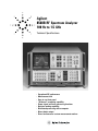
1
Agilent
8568B RF Spectrum Analyzer
100 Hz to 1.5 GHz
Technical Specifications
•
•
•
•
•
•
•
•
•
Exceptional RF performance
Measurement aids
Easy-to-use front panel
“On-board” computing capability
Power signal and trace processing functions
Decision-making capability
Distributed processing with a computer
Direct plotter output
Stores and executes custom measurement routines
2
Make Precise Measurements
Outstanding performance
A sophisticated phase lock system combines “synthesizer-like” tuning and
frequency accuracy with superior local oscillator spectral purity to make
narrow resolution bandwidths practical at RF frequencies and virtually
eliminate long-term drift. This system is administered by an internal
microcomputer which also makes possible powerful operational features
described in later pages.
Frequency measurement range
Measurement accuracy
Amplitude measurement range
The frequency measurement range
extends from 100 Hz to 1500 MHz
with dc and ac coupled inputs. The
analyzer's measurement capability
extends from RF down to audio
frequencies
High repeatability and features such
as tunable marker with frequency
count allow measurements to be made
more accurately and conveniently
than ever before.
The amplitude measurement range
extends from +30 dBm to –135 dBm
with 90 dB calibrated display,
and the input is protected from
accidental overload. Calibration
units can be selected from dBm,
dBmV, dBµV, and volts. The analyzer
measures signal levels as low as
32 nV (across 50 ohms).
Less than 1 x lO–9/day frequency
error, together with spectrum
analyzer selectivity, make counter
frequency accuracy possible even
when measuring small signals in the
presence of large ones. An internal
error correction routine reduces the
amplitude measurement uncertainty
due to changes in various analyzer
controls.
Under automatic control, the
analyzer's exceptional repeatability
may be used to further characterize
sources of measurement uncertainty,
and thereby enhance accuracy.
3
Make Precise Measurements – continued
Resolution bandwidth
Single sideband phase noise
Dynamic range
10 Hz to 3 MHz resolution bandwidths
are used in a 1, 3, 10 sequence. An
appropriate bandwidth is always
available to provide proper
resolution for any frequency span.
Single sideband phase noise is > 80
dB below the peak of a CW signal
at frequency offsets > 30 times the
resolution bandwidth setting, for
resolution bandwidths < 300 Hz.
Single sideband phase noise is
typically > 80 dB down and 200 Hz
away in a 10 Hz resolution bandwidth
at 1500 MHz.
The spurious-free dynamic range
measures > 80 dB with < –50 dBm
signal levels at the input mixer.
Harmonic and intermodulation
distortion products can typically
be measured > 90 dB below the peak
of a signal.
A narrow 10 Hz bandwidth makes
possible the resolution of 50 Hz
sidebands that are > 60 dB below
the peak of a 500 kHz signal, while
internal line-related sidebands
remain below the filter response.
Wide 1 and 3 MHz bandwidths with
"Gaussian" shapes improve sensitivity
and transient behavior when
measuring impulse noise, such as
electromagnetic interference, or
demodulating wideband spectra.
4
Get Acquainted Fast
Easy-to-use front panel
The front panel concept of the Agilent 8568B is innovative in two respects:
a comprehensive CRT readout that puts all the information where a user
needs it, and interactive function and data controls that make setting function
values very convenient.
Step keys
Step keys increment or decrement
function values have a logical amount,
depending upon the functions
selected and the display scaling.
CRT display
To set Its value
The 8568B display is fully annotated,
and even includes a function for
user-defined titles. The digital
display flicker- and parallax-free,
and can be transferred directly to
a plotter.
After activating a function, use the
DATA controls to alter the current
setting to the value you want.
Numeric/unit keypad
A numeric/unit keypad allows
precise entry of a function when a
specific setting is desired.
For example:
To increase the center frequency,
press [CENTER FREQUENCY],
turn [KNOB] or press [UP ARROW];
or, to set the center frequency
precisely to 1.5 GHz, press:
[CENTER FREQUENCY] [1] [.]
[5] [GHz].
Multi-purpose data controls
The front panel is logically designed
and easy to operate. The value of
any function on the instrument can
be set using a knob, step keys, or
numeric/unit keypad.
To activate a function
Activate a function simply by
pressing the appropriate key, such
as [FREQ] [SPAN] or [RES BW].
The value of the active function
most recently activated is indicated
on the CRT.
Knob
The knob changes the active function
with a “continuous” feel. It always
has a comfortable sensitivity for the
chosen range.
5
Get Acquainted Fast – continued
Front panel softkeys
Make your own front panel functions by defining softkeys, up to 58 characters
in length, directly from the front panel. Any analyzer command can be put
into a softkey, including program flow commands such as REPEAT and UNTIL,
and new firmware commands such as PEAKS. You can even define a softkey
that will execute other softkeys. Measurements that require several front
panel functions can be incorporated into one softkey to save time and
simplify measurements.
How to define measurement routines from the front panel
These four steps illustrate how easy it is to define a softkey that finds the
highest signal in a given span and “auto zooms” to a span of 100 kHz.
1. Select the commands
Use the GP-IB commands that are
necessary to accomplish this task;
in this case, MKPK HI (Peak Search),
MKTRACK ON (Signal Track On),
SP100KZ (Set Frequency Span to
100 kHz), TS (Take Sweep), and
MKRL (Bring the Signal to the
Reference Level).
2. “Type”commands into the
title block
To put the group of commands in a
softkey, “type” them into the title
block of the CRT. To do this, press
[SHIFT] E[AUTO]. This puts the
analyzer in the title mode so when
you press a front panel key, the letter
above the key appears in the upper
left corner of the CRT. Type in MKPK
HI,MKTRACKON,SP100KZ,TS,MKRL.
Press [NORMAL] (next to [SHIFT])
to terminate the title mode.
3. Store commands in RAM
To enter the commands in a softkey,
press [SHIFT] [2] [6] [kHz]. This
stores the commands in the RAM
of the analyzer under softkey 26.
(Softkeys can be labeled with any
number from 1 to 999.) Note: If “Save
Lock” appears in the active function
block on the center of the CRT, press
[SHIFT] [RECALL] and repeat the
key sequence [SHIFT] [2] [6] [kHz].
(Save Lock is a memory protection
function. For more information on
this feature, refer to page 8.)
6
4. Execute the softkey
Now you have a new front panel
function on the analyzer that
“autozooms” on a signal. This
measurement used to require eight
front panel keystrokes; now they
are all in one softkey. To execute it,
press [SHIFT] [2] [6] [HZ]. Notice
that “Softkey 26” appears in the
active function block of the CRT.
You can also define measurement
routines via GP-IB using a computer.
A computer provides the keyboard,
editing. and formatting capabilities
not available on the front panel of
the analyzer. This makes it possible
to enter into the analyzer softkey
routines greater than 58 characters
in length. This method is discussed
in more detail on page 13.
Complete Your Measurements Quickly and Easily
Operator-oriented features
It’s easy to operate the 8568B. It takes only a few functions to make a basic
signal measurement, and there are many functions available that make
sophisticated measurements as easy to perform as simpler ones.
Basic operation
To start
Press either the [0 to 1.5 GHz] or
[INST PRESET] keys to view the
desired frequency range. Both spans
set all the control states to convenient
preset values (e.g.,0 to 1.5 GHz span,
0 to –90 dBm amplitude range, etc.).
To measure
To measure a signal of interest,
follow this basic sequence:
1.
2.
3.
First. press [CENTER FREQUENCY]
and position the signal at the center
of the screen using one of the data
controls (e.g., the knob, step keys,
or the numeric keypad).
Second, press [FREQUENCY SPAN]
and, using the data controls, reduce
the, displayed frequency range.
Third, press [REFERENCE LEVEL.]
and raise the signal under test to
the top graticule line of the CRT.
Coupled functions
Save control settings
The resolution bandwidth, video
bandwidth, and sweeptime are
coupled to the frequency span for
an optimum calibrated display.
RF attenuation and reference level
functions are coupled to insure a
specific input m mixer drive level.
These functions can be uncoupled
and set manually. A warning will
appear on the CRT if the frequency
or amplitude becomes uncalibrated.
Once the analyzer controls have been
adjusted for a particular measurement,
all settings can be saved (or “learned”)
and later called to repeat the
measurement by accessing one of
the six storage registers as follows:
[SAVE] [5], then [RECALL] [5].
4.
The signal’s amplitude and frequency
can be read directly off the CRT.
You can lock settings in registers and
in softkeys with the Save Lock function.
To execute it, press [SHIFT] [SAVE].
This memory protection function
prevents new register and softkey
settings from being stored, so the
present settings are not erased. To
unlock registers and softkeys. and
remove the memory protection
function press [SHIFT] [RECALL],
7
Complete Your Measurements Quickly and Easily – continued
Direct plotter output
All trace, graticule, and annotation
information displayed on the CRT
can be plotted without the aid of a
controller. Simply connect the plotter
via GP-IB to the 8568B (set plotter
address to 705) and press the
LOWER LEFT key on the front panel.
Marker-aided measurements
The tunable marker makes basic signal measurements easily and accurately
by measuring signals directly. It also speeds the process of zooming in on a
portion of the frequency spectrum.
Direct measurements
Relative measurements
Multiple markers
[NORMAL] activates a tunable marker
whose amplitude and frequency are
displayed on the CRT. Signals can
be measured directly by tuning the
marker along the trace to the peak
of the signal. Internal commands
allow moving the marker to the
highest signal, next highest signal,
and next left or next right signal.
A second marker for making relative
measurements can be generated by
pressing [DELTA]; the difference
in amplitude and frequency between
the two markers is numerically
displayed on the CRT. The reference
frequency need not be displayed.
This feature is especially convenient
when comparing various spectral
component levels to a carrier or
fundamental to determine percent
modulation or distortion.
Up to four markers can be placed
on the display to make direct and
relative measurements at the same
time. Each marker reads the amplitude
and frequency value of its position on
the display. The markers are activated
individually and can respond to
any of the marker commands when
activated. While one marker is active,
relative measurements can be made
with the other three markers.
[FREQ COUNT] eliminates the
need for centering the marker by
displaying the frequency of the
signal on whose response the marker
is tuned — to counter accuracy.
8
Simplify Your Signal Analysis
Measurement aids
Amplitude and frequency offset
Peak search and signal track
Noise density measurement
The amplitudes and frequencies
displayed on the CRT can be offset by
any desired amount. This function
can normalize amplitudes and
frequencies to a standard, such
as a pilot tone, or reflect a signal's
parameters prior to amplification
or frequency conversion.
Zoom in quickly to the highest
amplitude response displayed on
the CRT using the functions [PEAK
SEARCH] and [SIGNAL TRACK].
Simply press [PEAK SEARCH] to
find the signal of greatest amplitude,
then press [SIGNAL TRACK] to move
the signal to center screen and hold
it there. To zoom in for a closer look,
press [FREQ SPAN] and reduce the
span using the data controls.
Gaussian noise power density can
be measured directly because all
correction and conversion factors are
incorporated into the noise density
function. The corresponding software
command automatically converts the
noise level at the marker to noise
power density (normalized to a 1 Hz
noise power bandwidth), and displays
the value on the CRT.
For example, consider this
measurement of 4 kHz test tones
relative to a 70 MHz pilot signal.
Rescaling the display by the pilot
signal frequency and level enables
the direct comparison between the
test tones and pilot signal in dBc.
9
Simplify Your Signal Analysis – continued
Trace functions
You can easily manipulate the way trace information is processed and displayed
by the 8568B. Using commands MPY (Multiply) and COMPRESS, traces
can be scaled in amplitude and compressed so more than one trace can be
independently displayed. Other trace processing functions, such as MEAN,
RMS, and STDEV, compute inside the analyzer the mean, RMS, and standard
deviation of trace amplitudes. This can reduce the amount of data that needs
to be transferred to a computer and reduce overall processing time.
Storage
Max hold
Compress
16k bytes of RAM are available
for trace storage, and up to eight
1001-point traces or sixteen 500-point
traces can be stored in RAM and
viewed on the CRT simultaneously
using the TRGRPH (Trace Graph)
command. Also available are three
independent storage buffers, traces A,
B, and C, and these too can be viewed
simultaneously. Traces A and B can
display signal responses in “real time”
when [CLEAR WRITE] is active, or
store them when [VIEW] is activated.
The largest amplitude occurring at
each of 1001 horizontal points across
the CRT over successive sweeps may
be displayed with [MAX HOLD].
Max Hold is useful for measuring
peak-to-peak residual FM and drift
over time, or when making swept
response measurements of filters
without a tracking source.
The COMPRESS command reduces
the length of a trace to a user-specified
length, so more than one trace can
be graphed on the analyzer screen.
Each trace can be generated from
completely different control settings.
A signal can be viewed in more than
one state, or several signals can be
viewed simultaneously. Traces that
are compressed require less memory
when stored, so more traces can be
stored. Compressed traces also take
less time to transfer to a computer.
Smooth
Low-level signals can be discerned
in one sweep using the SMOOTH
command. SMOOTH makes
measurements much faster than
digital averaging, because multiple
sweeps need not be taken. Like
digital averaging, SMOOTH does not
require an increase in sweeptime, so
it is also faster than video filtering.
10
Get Results, Mot Just Data, Using High-Level Signal
and Trace Processing Tools
The built-in, high-level functions of the 8568B provide signal and trace
processing tools that increase measurement capability and speed the
development of measurement programs. Signal processing tools such as
PWRBW (finds the power bandwidth of a signal) and PEAKS (identifies
nil responses on the display) allow data processing to be performed by the
analyzer without an external computer. Trace processing functions such as
RMS (finds the RMS value of a trace) and MPY (multiplies two traces, point
by point) eliminate long delays for transferring data to a computer, since
they are performed internally. Some functions process and store data in
the analyzer’s RAM. Others allow more than one active trace to be displayed
simultaneously.
By combining these functions, application-specific routines can be defined,
usually from a controller, and executed as front panel softkeys or as
computer-controlled routines. The examples below illustrate some application
areas which can be addressed.
PEAKS identifies all responses on the display
FFT performs a fast fourier transform
PWRBW returns the power bandwidth of a signal
Surveillance
Amplitude modulation analysis
Mobile radio
Signals can be monitored in any
user-specified band using the built-in
PEAKS routine. PEAKS identifies the
number of signal responses above a
threshold and records measurement
data on each signal identified, Using
PEAKS with other functions, trace
information and measurement data
can be simultaneously displayed.
Measurement data can also be
transferred to a system controller
printer, or plotter.
Previously, signals with very low
modulation rates and low modulation
indices could not be measured
because of resolution limitations
in the frequency domain. Now, with
the FFT function, the modulation
frequencies and distortion can be
easily measured. FFT also enables
accurate measurement of AM in the
presence of incidental phase angle
modulation.
The power bandwidth of many
types of signals can be calculated
internally with the PWRBW function.
For example, the modulation
bandwidth of an FM transmitter
can be measured for a user-specified
“percent of power” value. PWRBW
is also useful for voice modulated
measurements in AM, SSB, and
FM systems.
11
Create "On-Board" Measurement Routines
Softkey programming lets you develop the analyzer's measurement
“personality” by allowing you to create custom firmware functions for
your measurement needs.
As described earlier, softkeys can be defined from the front panel. However,
the following example illustrates how an operator can us a computer to
create longer or more complex measurement routines within a program
and then transfer all the data commands to the analyzer’s non-volatile RAM.
Once stored in memory, these routines can be easily executed from the
front panel by pressing three buttons, or “called” from a computer.
The following program defines a function called Z__OOM.
Lines 10-40 define Z__OOM as the
fund ions specified in lines 20 and
30. Line 50 assigns Z__OOM to softkeys 6 for front panel execution.
To execute
Via Computer
Type: OUTPUT 718; “Z__OOM”
Press: EXECUTE
Via Front Panel
Press: [SHIFT] [6] [HZ]
Define softkey routines that make decisions
The program flow commands of the Agilent 8566B (REPEAT/UNTIL,
IF/THEN/ELSE/ENDIF) allow you to create complete measurement or data
processing routines that can be executed in the analyzer without the use
of an external computer. This frees the computer to handle other system
instrumentation, or carry out additional data processing.
Use the command flow functions to
monitor a desired signal level. If the
signal goes below the specified level,
alert a computer by setting an GP-IB
service request. This will interrupt
current computer operations and
allow appropriate action to be taken.
12
Combine Processing Tools and Softkeys to
Solve Complex Measurement Tasks
Here are a few examples of measurements that can be be performed by
programs stored in the analyzer’s RAM.
Broadband monitoring
Percent modulation analysis
Harmonic distortion
Define a softkey that will continuously
monitor multiple bands of interest
and execute a fast sort on signals.
Include a command to zoom in
on a desired signal for more detailed
analysis. Such is softkey is ideal for
site monitoring and surveillance.
The analyzer can process and
provide immediate measurement
results without computer interaction.
In a production line environment,
this can completely eliminate the
need for a computer at each test
station. For repetitive testing, an
experienced technician can design
a measurement routine to be
“downloaded” into the analyzer.
The routine can be easily executed
and the results easily interpreted
by a less experienced operator.
Measurements which c:an be
extremely tedious when performed
manually, such as harmonic
distortion, are much easier when
performed internally via softkey.
Develop a routine that checks the
stability of a signal, eliminates any
internal distortion, and computes
and displays the the results on the
analyzer. Or, if desired, the results
of the measurement can be passed
on to a computer for further data
processing and storage.
SSB radio testing
Improve test productivity by leading
the operator through all aspects of
the test. Design an internal routine
that can pause to show a test setup,
continue until fine adjustments need
to be made, make the necessary test
measurements, and display the test
results on the analyzer screen.
13
Automatic Test System
The 8568B + PC = unparalleled measurement capability
Combine softkey routines with system
software to save I/O time and give you
the power of distributed processing.
Softkey routines can perform
measurement tasks measurement
tasks and process data inside the
analyzer to help minimize program
run times.
Enhance your program development
with the 85863A BASIC subprogram
library. This software package
provides high-level software
routines to help you develop custom
programs for specific applications.
14
EMI Measurement Capability
• The ideal EMI diagnostic tool
• Measurement software for fully automated EMI testing
• The Agilent 85685A RF preselector converts the
Agilent 8568B/85650A into a CISPR receiver
• Accessories available for making complete EMI test systems
International Special Des Perturbations
Radioélectriques) publication number
16 recommendation. The preselector
provides overload protection and
improves measurement sensitivity.
EMI regulations can be divided into
two general categories: military
regulations and commercial
regulations. Commercial regulations
have been heavily influenced by the
recommendations of CISPR, a special
committee of the International
Electrotechnical Commission (IEC).
Many international groups have
adopted in part the recommendations
of CISPR, including the Federal
Communications Commission (FCC)
in the USA and the Verband Deutscher
Electrotechniker (VDE) in Germany.
There are numerous military EMI
standards, but the most widely used
of these is Military Standard 461/462
(developed by the Armed Forces of
the USA).
The spectrum analyzer has long burn
a useful tool in evaluating electromagnetic interference (EMI) spectra
for troubleshooting and preliminary
qualification testing. The 8568B
spectrum analyzer, with high
performance and full programmability,
allows difficult and time-consuming
EMI compliance tests to be completed
automatically.
The spectrum analyzer’s ability to
display wide frequency spans provides
“quick-look” capability, making it
effective for locating FMI “hot spots”
manually. Full programmability and
the graphics display capability for
log pints, limit lines and hard copies
make the 8568B a very powerful and
effective measurement tool for EMI
applications requiring automation.
The 85864A FMI Measurement
Software program, added to the
capability of the 8568B, is a powerful
combination for military standard
(MIL-STD) and commercial (FCC,
VDE, CISPR) EMI testing. Many common EMI tests are provided in the
85864A software library on discs, and
a custom test can be implemented
within minutes for individual testing
needs. The software has a variety of
analysis features for diagnosing or
identifying the measured emissions.
You can “zoom to local” and identify
the type or source of emission, print
the peak responses of the measured
emissions above a desired threshold
level, perform a quasi-peak
measurement over a selected
portion of the measurement range,
and mark Specific responses for
identification on a report. The
858U4A also provides hardcopy
output (plotted or printed) and disc
storage capability for saving data or
new test setups.
The procedures for making military
standard (MIL-STD) measurements are
different from the procedures required
for making CISPR measurements.
The 8568B spectrum analyzer has
the capability to meet MIL-STD
measurements and, when used
with the 85650A quasi-peak adapter,
has the capability to meet the
requirements of both CISPR and
MIL-STD measurements. The graph
shown below is a test result of an
FCC measurement and illustrates
how an 8568B-based automatic
measurement system can use the
spectrum analyzer’s custom graphics
and hard copy capabilities.
The 85685A RF preselector converts
the 8566B and 85650A quasi-peak
adapter into an EMI receiver
conforming to CISPR (Comité
15
Specifications
Performance summary
Specifications describe the instrument's warranted performance over the temperature range 0° to 55 °C (except where noted.) Supplemental characteristics
are intended to provide information useful in applying the instrument by giving typical, but non-warranted, performance parameters. These are denoted as
"typical," "nominal," or "approximately." Where specifications are subject to minimization with the error correction routine, corrected limits are given unless
noted. (The error correction routine is a built-in routine using the CAL OUTPUT signal and pressing SHIFT W then SHIFT X. The message CORR'D appears
in the CRT display when the correction is being applied.)
Frequency
Sweep
Measurement range
Sweep time
100 Hz to 1500 MHz dc coupled and
100 kHz to 1500 MHz ac coupled.
20 msec full span to 1500 sec full span. Zero frequency span,
1 µsec full sweep to 1500 sec full sweep.
Resolution
3 dB bandwidths of 10 Hz to 3 MHz in a 1, 3, 10 sequence.
Inputs
Spectral purity
Noise sidebands > 80dB below peak of CW signal at frequency
offsets ≥ 30 x resolution bandwidth setting, for resolution
bandwidths ≤ 300 Hz.
Accuracy
Frequency reference accuracy (aging rate)
< 1 x 10⁻⁹/day (2 x 10⁻⁷/yr.). After 30-day warmup.
Center frequency
±(2% of frequency span + frequency reference accuracy x
tune frequency + 10 Hz) using error correction.
Frequency span
Spans > 1 MHz, ±(2% of indicated separation between
two points +0.5% of span); spans ≤ 1 MHz, ±(5% of indicated
separation +0.5% of span).
Marker
Normal: Center frequency accuracy + frequency span
accuracy between the marker and center frequency.
Freq Count: Frequency reference accuracy x displayed
frequency ± frequency counter resolution (spans ≤ 100 Hz).
RF inputs
100 Hz to 1500 MHz, 50 Ω dc coupled (BNC fused); and
100 kHz to 1500 MHz, 50 Ω ac coupled (type N).
Max input level
ac: +30 dBm (1 watt) continuous power: 100 watts, 10 µsec
pulse into > 50 dB attenuation.
dc; 0 volts dc coupled input and ±50 volts for ac coupled input.
Attenuator
70 dB range in 10 dB steps.
Outputs
Display
X, Y, and Z outputs for auxiliary CRT display.
Recorder
Horizontal sweep output (X), video output (Y), and
penlift/blanking output (Z) to drive an X-Y recorder.
Remote operation
Amplitude
Measurement range
–135 dBm to +30 dBm or equivalent in dBmV, dBµV; 40 nV to 7 V.
Dynamic range
Spurious responses
Second harmonic distortion and third order intermodulation
distortion > 70 dB below signal levels ≤ –30 dBm at the
input mixer.
Average noise level
< –135 dBm in 10 Hz resolution bandwidth.
Accuracy
Calibrator uncertainty
±0.2 dB.
Frequency response uncertainty
±1.0 dB, 100 Hz to 1500 MHz.
16
All analyzer control settings (with the exception of video trigger
level, focus, align, intensity, frequency zero, amplitude cal, and line
power) may be programmed via the interface bus (GP-IB).
Specifications
See definition of specifications and supplemental characteristics on page 16.
Frequency
Bandwidth selectivity
60 dB/3 dB bandwidth ratio:
< 15:1 3 MHz to 100 kHz
< 13:1 30 kHz to 10 kHz
< 11:1 3 kHz to 30 Hz
60 dB points on 10 Hz bandwidth are separated by < 100 Hz.
Bandwidth shape
Synchronously tuned (approximately Gaussian).
Measurement range
100 Hz to 1500 MHz through two RF inputs: 100 Hz to
1500 MHz dc coupled and 100 kHz to 1500 MHz ac coupled.
Display values
Center frequency
0 Hz to 1500 MHz.
Variable from data knob or numeric/unit keyboard
in approximately 1% increments.
Frequency reference accuracy:
Aging rate: < 1 x l0E–9/day and < 2.5 x l0E–7/year
Warm-up time (after less than 24 hours with line
power disconnected):1
< 72 hours to meet aging rate specification
Warm-up time (after line power is disconnected
indefinitely):1
30 days to meet aging rate specification
Temperature stability: < 7 x 10E–9 over the 0 ° to 55 °C range.
Readout accuracy
Span ≥ 100 Hz: ±(2% of frequency span + frequency
reference accuracy x tune frequency +10 Hz) after
adjusting freq zero at stabilized temperature.
Zero frequency span
Resolution
Accuracy: Freq ref
Readout
bandwidth
accuracy x tune freq +
resolution
10 to 300 Hz
10 Hz
1 Hz
1K to 3kHz
100 Hz
10 Hz
10K to 3 MHz
1 kHz
100 Hz
Frequency span
100 Hz to 1500 MHz over 10-division CRT horizontal axis.
Variable from data knob, or numeric/unit keyboard in
approximately 1% increments; step keys change span
in a 1,2, 5 sequence.
In zero span, the instrument is fixed tuned at the center
frequency.
Full span (0 to 1500 MHz) is immediately executed with
0 to 1.5 GHz or INSTR PRESET keys.
Frequency span accuracy: For spans > 1 MHz, +(2% of the
indicated frequency separation between two points
+0.5% span); for spans ≤ 1 MHz, ±(5% of frequency
separation + 0.5% span).
Start-stop frequency
Readout accuracy: center frequency accuracy
+ 1/2 frequency span accuracy.
Figure 1. Typical spectrum analyzer resolution
Marker
Normal
Displays the frequency at the horizontal position of the
tunable marker.
Accuracy: Center frequency accuracy + frequency span
accuracy between the marker and center frequency.
Peak search positions the marker at the center of the
largest signal response present on the display to within
± 10% of resolution bandwidth.
∆
Displays the frequency difference between the stationary
and tunable markers. Reference frequency need not be
displayed.
Accuracy: Same as frequency span accuracy; in the
frequency count mode, twice the frequency count
uncertainty plus drift during the period of the sweep
(see STABILITY DRIFT).
Freq Count
Displays the frequency of the signal on whose response the
marker is positioned.
Resolution
Resolution bandwidth
3 dB bandwidths of 10 Hz to 3 MHz in a 1, 3,10 sequence.
Bandwidth may be selected manually or coupled to
frequency span.
Bandwidth accuracy: Calibrated to:2
±10%, 1 MHz to 3 kHz bandwidths.
±20%, 1 kHz to 10 Hz. 3 MHz bandwidths.
1 Line voltage disconnected without power to the frequency reference. When the
analyzer is in “stand by”, the frequency reference temperature is maintained at
a steady state. Frequency accuracy is then subject to the standard instrument
warm-up period indicated in the General Specifications section.
2 30 kHz and 100 kHz bandwidth accuracy figures only applicable ≤ 90% relative
humidity.
17
Specifications
See definition of specifications and supplemental characteristics on page 16.
The marker must be positioned at least 20 dB above the
noise or the intersection of the signal with an adjacent
signal and more than four divisions up from the bottom of
the CRT. Counter resolution is normally a function of
frequency span but may be specified directly using SHIFT =.
Accuracy: For spans < 100 kHz: frequency reference
accuracy x displayed frequency ±2 x frequency
counter resolution.
For spans > 100 kHz but ≤ 1 MHz: freq ref accuracy x
displayed frequency ±(10 Hz + 2 x frequency counter
resolution).
For spans > 1 MHz: ± (10 kHz + frequency counter resolution).
Stability
Residual FM
< 3 Hz peak-to-peak for sweep time ≤ 10 sec; span
< 100 kHz, resolution bandwidth ≤ 30 Hz, video bandwidth
≤ 30 Hz.
Drift
(After 1-hr. warm-up at stabilized temperature)
Frequency spans ≤ 100 kHz, < 10 Hz/minute of SWEEPTIME;
> 100 kHz but < 1 MHz, < 100 Hz/minute of SWEEPTIME;
> 1 MHz, < 300kHz/minute of SWEEPTIME.
Because of a correction on retrace, analyzer drift only
occurs during the period of one sweep.
Spectral purity
Noise sidebands
Offset
SSB phase noise
from carrier
dBc (1 Hz BW)
300 Hz
–90
3 kHz
–100
30 kHz
–107
Refer to Figure 2 for typical SSB noise limits.
Amplitude
Measurement range
–135 dBm to +30 dBm.
Displayed values
Scale
Over a 10-division CRT vertical axis with the reference level
(0 dB) at the top graticule line.
Calibration
Log: 10 dB/div for 90 dB display from reference level
5 dB/div for 50 dB display
expanded from
2 dB/div for 20 dB display
reference level
1 dB/div for 10 dB display
Linear: 10% of reference level/div when calibrated
in voltage.
Fidelity
CRT linearity and log or linear fidelity affect amplitude
accuracy at levels other than the reference level.
Log: (over 0 to 90 dB display)
Incremental Accuracy: ±0.1 dB/dB over 0 to 90 dB display
Maximum cumulative error: (from the reference level)
3 MHz to 30 Hz Res BW
< ±1.0 dB max over 0 to 80 dB display, 20° to 30 °C
< ±1.5 dB max over 0 to 90 dB display, 10 Hz Res BW
2.1 dB max over 0 to 90 dB display
Linear: ±3% of Reference Level.
Reference level
Range
Log: +30.0 to –99.9 dBm or equivalent in dBmV, dBµV, volts.
Expandable to +60.03 to –119.9 dBm (–139.9 dBm
≤ 1 kHz resolution bandwidth) using SHIFT I.
Linear: 7.07 volts to 2.2 µvolts full scale.
Expandable to 223.63 volts to 2.2 µvolts (0.22 µvolts
< 1 kHz resolution bandwidth) using SHIFT I.
Signals at the reference level in log translate to
approximately full scale signals in linear, typically within
± 1 dB at room temperature.
Accuracy
The sum of the following factors determines the accuracy
of the reference level readout. Depending upon the
measurement technique followed after calibration, some
of these sources of uncertainty may not be applicable.
An internal error correction function reduces the uncertainty
introduced by analyzer control changes from a state defined
during the calibration of the instrument when SHIFT W is
executed just prior to the signal measurement (i.e., at the
same temperature) within the 20 ° to 30 °C range. All
uncertainties, corrected and uncorrected, assume the
analyzer has had a minimum of one hour warm-up time.
Calibrator uncertainty
±0.2 dB.
]
Figure 2. Typical SSB noise versus offset from carrier
Power line related sidebands
> 85 dB below the peak of a CW signal.
18
3 Maximum input must not exceed +30 dBm damage level.
Specifications
See definition of specifications and supplemental characteristics on page 16.
Frequency response (flatness) uncertainty
≥ 10 dB RF Attenuation
Input 1: ±1dB, 100 Hz to 500 MHz; ± 1.5 dB 100 Hz
to 1500 MHz.
Typically: ±0.75 dB 100 Hz to 500 MHz; ±1.0 dB 100 Hz
to 1500 MHz; +1, –4 dB 1500 MHz to 1650 MHz.
Input 2: ±1 dB, 100 kHz to 1500 MHz.
Typically: ±0.7 dB 100 kHz to 1500 MHz; +1, –4 dB
1500 MHz to 1650 MHz.
Amplitude temperature drift
At –10 dBm reference level with 10 dB input attenuation
and 1 MHz resolution bandwidth, ±0.05 dB/°C
(eliminated by recalibration).
Input connector switching uncertainty
±0.5 dB when calibration and measurement do not
use same RF input.
Input attenuation switching uncertainty
±1.0 dB over 10 dB to 70 dB range.
Resolution bandwidth switching uncertainty4
(referenced to 1 MHz bandwidth) — corrected (uncorrected)
Resolution BW
20 to 30 °C
0 to 55 °C
(After 1-hour warm-up)
10 Hz
±1.1 dB (±2.0 dB)
(±4.0 dB)
30 Hz
±0.4 dB (±0.8 dB)
(±2.3 dB)
100 Hz to 1 MHz
±0.2 dB (±0.5 dB)
(±2.0 dB)
3 MHz
±0.2 dB(±1.0 dB)
(±2.0 dB)
Log scale switching uncertainty
±0.1 dB corrected (±0.5 dB uncorrected).
IF gain uncertainty — corrected (uncorrected)
Assuming the internal calibration signal is used to
calibrate the reference level at –10 dBm and the input
attenuator is fixed at 10 dB, any changes in reference
level in the following ranges will contribute IF gain
uncertainty:
Reference level
20 to 30 °C
0 to 55 °C
0 to –55.9 dBm
10 Hz Res BW
±1.0 dB (±1.6 dB)
(±2.0 dB)
≥ 30 Hz Res BW
0 dB (±0.6 dB)
(± 1.0 dB)
–56.0 to –129.9 dBm
10 Hz Res BW
≥ 30 Hz Res BW
(±2.0 dB)5
(±1.0 dB)5
(±2.5 dB)
(±1.5 dB)
Each 10 dB decrease (or increase) in the amount of input
attenuation at the time of calibration and measurement
will cause a corresponding 10 dB decrease (or increase)
in the absolute reference level settings described above.
RF gain uncertainty (due to 2nd LO shift)
±0.1 dB corrected (±1.0 dB uncorrected).
Error correction accuracy (applicable when SHIFT W
and SHIFT X are used):
±0.4 dB.
Reference lines
Accuracy
Equals the sum of reference level accuracy plus the scale
fidelity between the reference level and reference line.
Dynamic range
Spurious responses
For total signal power of < –40 dBm at the input mixer of
the analyzer, all image and out-of-band mixing responses,
harmonic and intermodulation distortion products are
> 75 dB below the total signal power for input signals
10 MHz to 1500 MHz, and > 70 dB below the total signal
power for input signals 100 Hz to 10 MHz.
Second harmonic distortion: For a signal –30 dBm at the
mixer and > 10 MHz, second harmonic distortion > 70 dB
down; 60 dB down for signals < 10 MHz. Refer to Figure 3
for typical second harmonic distortion levels.
Figure 3. Optimum dynamic range
Third order intermodulation distortion: For two signals
each –30 dBm at the mixer, third order intermodulation
produces:
Signal
Center
Relative
separation
frequency
distortion
T.O.I.
< 100 kHz
> 100 kHz
< –70 dBc
+5 dBm
> 100 kHz
> 10 MHz
< –80 dBc +10 dBm
4 30 kHz and 100 kHz bandwidth switching uncertainty figures only applicable
≤ 90% relative humidity.
5 Correction only applies over the 0 dBm to –55.9 dBm range.
19
Specifications
See definition of specifications and supplemental characteristics on page 16.
To establish a particular spurious-free dynamic range (in the
coupled attenuator mode), the input mixer drive level is
specified using SHIFT, (comma) and the desired level is
entered through the keyboard.
Residual responses (no signal at input)
< –105 dBm for frequencies > 500 Hz with 0 dB input
attenuation.
Gain compression
< 0.5 dB for signal levels < –10 dBm at the input mixer.
Average noise level (sensitivity)
Displayed < –135 dBm for frequencies > 1 MHz, < –112 dBm
for frequencies ≤ 1 MHz but > 500 Hz with 10 Hz resolution
bandwidth (0 dB input attenuation, 1 Hz video filter).
Refer to Figure 4 for typical noise levels.
When SHIFT M is used with the marker the displayed noise
level is adjusted to reflect the RMS noise level/1 Hz BW
which is typically < –142 dBm/1 Hz and < –119 dB/1 Hz
respectively for frequencies > 1 MHz and ≤ 1 MHz but > 500 Hz.
Sweep
Sweep time
Continuous
Sequential sweeps initiated by the trigger: 20 msec full span
to 1500 sec full span in 1,1.5,2,3,5,7.5,10 sequence.
Accuracy: Sweep time ≤ 100 sec, ±10%; >100 sec, ±20%.
Zero frequency span
Accuracy: same as continuous.
Marker (sweeps ≥ 20 msec only)
Normal: Displays time from beginning of sweep to
marker position.
Accuracy: Sweep time settings ≥ 20 msec but ≤ 100 sec,
±10% x (indicated time/sweep time setting);
settings > 100 sec, ±20% x (indicated time/sweep
time setting).
∆: Displays time difference between stationary and
tunable marker.
Accuracy: same as normal.
Inputs
RF inputs
The standard instrument configuration is as follows:
Input #1
100 Hz to 1500 MHz, 50 Ω, BNC connector (fused); dc coupled.
Reflection coefficient: Typically < 0.20 (1.5 SWR) to 500 MHz,
< 0.33 (2.0 SWR) 500 MHz to 1500 MHz; ≥ 10 dB input
attenuation.
Fuse blow time: < 0.1 sec for input > 35 dBm (250 mA).
Figure 4. Typical sensitivity vs. input frequency
Marker
Normal
Displays the amplitude at the vertical position of the
tunable marker.
Accuracy: Equals the sum of the calibrator uncertainty,
reference level uncertainty, and scale fidelity between the
reference level and marker position.
∆
Displays the amplitude difference between the stationary and
tunable markers. Reference frequency need not be displayed
Accuracy: Equals the sum of scale fidelity and frequency
response uncertainty between the two markers.
20
Input #2
100 kHz to 1500 MHz, 50 Ω, Type N connector; ac coupled.
Reflection coefficient: Typically < 0.20 (1.5 SWR);
> 10dB input attenuation.
LO emission (typical)
Typically < –75 dBm (0 dB RF ATTEN).
Isolation (typical)
> 90 dB between inputs.
Also available: Input #1, 100 Hz to 1500 MHz, 75 Ω.
BNC connector, dc coupled (Option 001).
Maximum input level
AC
Continuous power, +30 dBm (1 watt); 100 watts, 10 µsec
pulse into > .50 dB attenuation.
DC
Input #1, 0 volts; input #2, ±50 volts
Specifications
See definition of specifications and supplemental characteristics on page 16.
Input attenuator
0 to 70 in 10 dB steps.
Damage level: +30 dBm (1 watt).
External sweep trigger input (rear panel)
Must be > 2.4 volts (5 volt max). 1 kΩ nominal input impedance.
External frequency reference input (rear panel)
Must equal 10 MHz ±50 Hz, 0 dBm (+10 dBm max.),
50 Ω nominal input impedance. Analyzer phase noise
performance may be degraded when an external frequency
reference is used.
Quasi-peak (rear panel; nominal values)
Video input: 0 to 2 volts. 139 Ω input impedance.
21.4 MHz IF input: Input is nominally –11 dBm with 10 dB input
attenuation. 50 Ω input impedance.
Outputs
Calibrator
20 MHz ±20 MHz x frequency reference accuracy.
–10 dBm ±0.2dB; 50 Ω.ß
Probe power
+15 V, –12.6 V; 150 mA max.
Powers Agilent 1121A ac coupled (useable only with input #2)
and Agilent 1120A dc coupled high impedance probes.
Auxillary (rear panel; nominal values)
Display (typical parameters)
X, Y and Z outputs for auxiliary CRT displays exhibiting
< 75 nsec rise times for X, Y and < 30 nsec rise time for
Z (compatible with 1300 Series displays). X, Y:
1 volt full deflection; Z: 0 to 1 V intensity modulation,
–1 V blank. BLANK output (TTL level > 2.4 V for blanking)
compatible with most oscilloscopes.
Recorder (typical parameters)
Outputs to drive all current X-Y recorders
(using positive pencoils or TTL penlift input).
Horizontal sweep output (X axis): A voltage proportional to
the horizontal sweep of the frequency sweep generator
that ranges from 0 V for the left edge to +10 V for the
right edge. 1.7 kΩ output impedance.
Video output (Y axis): Detected video output (before A-D
conversion) proportional to vertical deflection of the
CRT trace. Output increases 100 mV/div from 0 to 1 V.
Output impedance ≤ 475 Ω.
Penlift output (Z axis; A blanking output, 15 V from 10 kΩ,
occurs during frequency sweep generator retrace; during
sweep, output is low at 0 V with 10 Ω output impedance
for a normal or unblanked trace (pen down).
LOWER LEFT and UPPER RIGHT push buttons calibrate the
recorder sweep and video outputs with 0,0 and 10,1 volts
respectively, for adjusting X-Y recorders. Pressing LOWER
LEFT with an GP-IB plotter connected will cause direct plot
of CRT information.
21.4 MHz IF
A 50 Ω, 21.4 MHz output related to the RF input to the analyzer.
In log scales, the IF output is logarithmically related to the
RF input signal; in linear, the output is linearly related. The
output is nominally –20 dBm for a signal at the reference level.
1st LO
2 to 3.7 GHz. > +4 dBm; 50 Ω output impedance.
Frequency reference
10.000 MHz, 0 dBm nominal; 50 Ω output impedance.
Quasi-peak (rear panel; nominal values)
Video output: 0 to 2 volts. < 139 Ω output impedance.
21.4 MHz IF output: Output is nominally –11 dBm
(with 10 dB input attenuation). 50 Ω output impedance.
Display
Cathode ray tube
Type
Post deflection accelerator, aluminized P31 phosphor,
electrostatic focus and deflection.
Viewing area
Approx. 9.6 cm vertically bv 11.9 cm horizontally
(3.8 in. x 4.7 in.).
General
Environmental
Temperature
Operating 0 ° to 55 °C, storage –40 ° to +75 °C.
EMI
8568B conducted and radiated interference is within the
requirements of Class A1c, RE02 of MIL STD 461B, VDE 0871,
and CISPR publication 11.
Warm-up time
Operation
Requires 30-minute warm-up from cold start, 0° to 55 °C.
Internal temperature equilibrium is reached after 2-hr.
warmup at stabilized outside temperature.
Frequency reference (typical)
Frequency reference aging rate attained after 30-day warmup
from cold start at 25 °C. Frequency is within 1 x 10⁻⁸ of final
stabilized frequency within 30 minutes.
Power requirements
50 to 60 Hz; 100, 120. 220 or 240 volts (+5%, –10%);
approximately 450 VA (40 VA in standby).
400 Hz operation is available as Option 400.
Battery storage
Lithium battery holds information in RAM for typically 1 year.
Weight
Total net, 45 kg (100 lb); Display/IF section, 21 kg (46 lb);
RF section. 24 kg (54 Ib). Shipping net, 72 kg (158 lb); Display/IF
section, 27 kg (60 lb); RF Section, 32 kg (70 lb); Manuals and
accessories, 13 kg (28 lb).
21
Specifications
See definition of specifications and supplemental characteristics on page 16.
NOTE:
Dimensions in millimetres and (inches)
(Allow 100 mm, 4 inch clearance at
rear panel for interconnect cables.)
Power requirements
400 Hz ±10% line frequency; 100 or 120 volts (+5%, –10%)
line voltage; 50 to 60 Hz power line frequency for service only,
not for extended periods.
Temperature range (operating)
0 ° to 55 °C. Restricted to 0 ° to 35 °C, 50 Hz to 60 Hz.
Mounting kits
Rack flange kit (Option 908)
Rack flange kit to mount instruments with handles (Option 913)
Rack mount slide kit (Option 010)
Meets EIA RS310-C Specification.
Extra manuel (Option 910)
Retrofit kit (8568A +01 K)
Remote operation
The standard 8568B operates on the interface bus (GP-IB).
All analyzer control settings (with the exception of VIDEO
TRIGGER LEVEL, FOCUS, ALIGN, INTENSITY, FREQ ZERO, AMPTD
CAL, and LINE power) are remotely programmable. Function
values, marker frequency/amplitude, and traces may be output;
CRT labels and graphics may be input.
LCL
Returns analyzer to local control, if not locked out by controller.
Service request
SHIFT r calls an GP-IB request for service.
Interface codes
SH-l, AH1, T6, L4, SR1, RL1, PPO, DC1, DT1, CO, E1.
Options
All specifications are identical to the standard 8568B except as noted.
75 Ω input impedance (Option 001)
RF input #1
100 Hz to 1500 MHz, 75 Ω, BNC connector; dc coupled,
not fused.
Average noise level (0 dBm input attenuation, 1 Hz video filter)
Noise level displayed on RF input #1 –129 dBm with 10 Hz
resolution bandwidth, frequencies >1 MHz; < –106 dBm
for frequencies ≤ 1 MHz, but > 500 Hz.
Residual responses (no signal at input)
< –99 dBm, input #1.
400 Hz power line frequency operation (Option 400)
Line related sidebands
> 75 dB below peak of CW signal.
Residual responses (no signal at input)
< –95 dBm for frequencies > 500 Hz: < –105 dBm for
frequencies > 2.5 kHz. 0 dB input attenuation.
22
Contains hardware and documentation to change an
85680A to an 85680B. Also includes BASIC operation
verification software for use with 9000 Series computers,
one 5 1/4-inch flexible disk, and one 3 1/2-inch micro
flexible disk.
Part numbers
Agilent 8568B spectrum analyzer
Option 001: 75 Ω (BNC), 100 Hz to 1500 MHz RF input #1
Option 400: 400 Hz power line frequency operation
Option 908: rack flange kit
Option 913: rack flange kit to mount instruments with handles
Option 010: rack mount slide kit (meets EIA RS310-C specification)
Option 910: extra manual
Accessories
Agilent 85650A quasi-peak adapter
Agilent 85685A RF preselector
Agilent 8568A +01 K retrofit kit
Agilent 8444A Option 059 tracking generator
Agilent 8447D preamplifier, 0.1 to 1300 MHz
Service kit for 8568B, P/N 08568-60005
Transit case
RF section P/N 1540-0602
IF section P/N 1540-0663
23
Agilent Technologies’ Test and Measurement Support,
Services, and Assistance
Agilent Technologies aims to maximize the value you
receive, while minimizing your risk and problems. We
strive to ensure that you get the test and measurement
capabilities you paid for and obtain the support you need.
Our extensive support resources and services can help
you choose the right Agilent products for your applications
and apply them successfully. Every instrument and system
we sell has a global warranty. Support is available for at
least five years beyond the production life of the product.
Two concepts underlie Agilent’s overall support policy:
“Our Promise” and “Your Advantage.”
Our Promise
Our Promise means your Agilent test and measurement
equipment will meet its advertised performance and
functionality. When you are choosing new equipment, we
will help you with product information, including realistic
performance specifications and practical recommendations
from experienced test engineers. When you receive your
new Agilent equipment, we can help verify that it works
properly and help with initial product operation.
Your Advantage
Your Advantage means that Agilent offers a wide range of
additional expert test and measurement services, which
you can purchase according to your unique technical and
business needs. Solve problems efficiently and gain a
competitive edge by contracting with us for calibration,
extra-cost upgrades, out-of-warranty repairs, and onsite
education and training, as well as design, system integration, project management, and other professional engineering services. Experienced Agilent engineers and technicians worldwide can help you maximize your productivity,
optimize the return on investment of your Agilent instruments and systems, and obtain dependable measurement
accuracy for the life of those products.
Agilent T&M Software and Connectivity
Agilent’s Test and Measurement software and connectivity
products, solutions and developer network allows you to
take time out of connecting your instruments to your computer with tools based on PC standards, so you can focus
on your tasks, not on your connections. Visit
www.agilent.com/find/connectivity
for more information.
For more information on Agilent Technologies’ products,
applications or services, please contact your local
Agilent office. The complete list is available at:
www.agilent.com/find/contactus
Phone or Fax
United States:
(tel) 800 829 4444
(fax) 800 829 4433
Canada:
(tel) 877 894 4414
(fax) 800 746 4866
China:
(tel) 800 810 0189
(fax) 800 820 2816
Europe:
(tel) 31 20 547 2111
Japan:
(tel) (81) 426 56 7832
(fax) (81) 426 56 7840
I
www.agilent.com/find/emailupdates
Get the latest information on the products
and applications you select.
24
Korea:
(tel) (080) 769 0800
(fax) (080)769 0900
Latin America:
(tel) (305) 269 7500
Taiwan:
(tel) 0800 047 866
(fax) 0800 286 331
Other Asia Pacific
Countries:
(tel) (65) 6375 8100
(fax) (65) 6755 0042
Email: [email protected]
Contacts revised: 9/17/04
Product specifications and descriptions in this document
subject to change without notice.
© Agilent Technologies, Inc. 1985, 2004
Printed in USA, September 29, 2004
5952-9394